Embed Size (px)
Citation preview

/ department of mathematics and computer science 1/47
LNMB Course
Asymptotic Methodsin Queueing Theory
Lecture 2, March 6, 2017
Rudesindo Núñez-Queija (CWI/UvA), Sem Borst (TU/e)
http://www.win.tue.nl/˜sem/AsQT/

/ department of mathematics and computer science 2/47
Course overview
Four main topics
• Large deviations and tail asymptotics
– Large-buffer asymptotics for light-tailed queues (today)
– Many-sources asymptotics (today)
– Large-buffer asymptotics for heavy-tailed queues (next week)
– Impact of service discipline on delay asymptotics (next week)
• Heavy-traffic analysis
• Perturbation analysis and time scale separation
• Fluid (and possibly diffusion) limits
/ department of mathematics and computer science 3/47
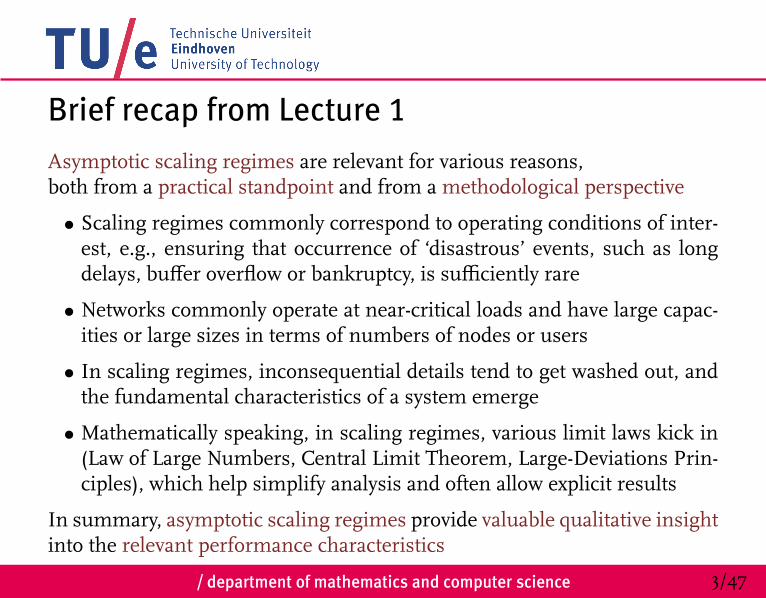
Brief recap from Lecture 1
Asymptotic scaling regimes are relevant for various reasons,both from a practical standpoint and from a methodological perspective
• Scaling regimes commonly correspond to operating conditions of inter-est, e.g., ensuring that occurrence of ‘disastrous’ events, such as longdelays, buffer overflow or bankruptcy, is sufficiently rare
• Networks commonly operate at near-critical loads and have large capac-ities or large sizes in terms of numbers of nodes or users
• In scaling regimes, inconsequential details tend to get washed out, andthe fundamental characteristics of a system emerge
• Mathematically speaking, in scaling regimes, various limit laws kick in(Law of Large Numbers, Central Limit Theorem, Large-Deviations Prin-ciples), which help simplify analysis and often allow explicit results
In summary, asymptotic scaling regimes provide valuable qualitative insightinto the relevant performance characteristics

/ department of mathematics and computer science 4/47
Lindley recursion for single-server queue
Consider a single-server queue (switch in a communication network) witha time-slotted operation and a finite buffer of size B for holding customers(data packets)
Denote by Qt the buffer content at the end of time slot t
Then the sequence (Qt)t∈Z satisfies the recursive relation
Qt = [Qt−1 + At − Ct]B0 ,
with [x]B0 = max{min{x, B}, 0}, and
• At : amount of traffic (e.g. number of packets) arriving into the bufferduring time slot t
• Ct : maximum amount of traffic (e.g. number of packets) that can beserved during time slot t

/ department of mathematics and computer science 5/47
Lindley recursion for single-server queue (ct’d)
Some observations and further assumptions
• The evolution of (Qt)t≥0 is only affected by the differential 1Qt = At −
Ct , and mathematically speaking it is sufficient to consider a recursionin terms of 1Qt only
• It will still be more insightful to keep track of the individual componentsAt and Ct separately, but we may as well assume that all the randomvariation is contained in At and that Ct ≡ C for all t
• We also assume B = ∞, so the recursive relation simplifies to
Qt = [Qt−1 + At − C]+, (1)
with [x]+ = max{x, 0} as before
• In addition, we assume that (At)t∈Z is sequence of independent andidentically distributed (i.i.d.) copies of a generic random variable A, withE{A} < C (because otherwise Qt →∞ with probability one)

/ department of mathematics and computer science 6/47
Lindley recursion for single-server queue (ct’d)
As the results for the stationary waiting-time distribution in the M/G/1queue reflect, the above recursive relation can be used to obtain the exactdistribution of the stationary buffer content distribution in various specialcases, and in particular the tail behavior, i.e., the behavior of P{Q > q} asq →∞ (Lecture 1)
However, we aim for asymptotic results in more general scenarios, and inparticular use large-deviations methods to determine the tail behavior (to-day’s focus)
/ department of mathematics and computer science 7/47
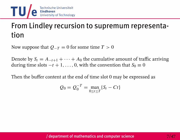
From Lindley recursion to supremum representa-tion
Now suppose that Q−T = 0 for some time T > 0
Denote by St = A−t+1 + · · · + A0 the cumulative amount of traffic arrivingduring time slots −t + 1, . . . , 0, with the convention that S0 ≡ 0
Then the buffer content at the end of time slot 0 may be expressed as
Q0 = Q−T0 = max
0≤t≤T{St − Ct}

/ department of mathematics and computer science 8/47
From Lindley recursion to supremum representation (cont’d)
This may be shown through induction or simply applying the recursive re-lation T times:
Q0 = max{Q−1 + A0 − C, 0}= max{max{Q−2 + A−1 − C, 0} + A0 − C, 0}= max{Q−2 + A−1 + A0 − 2C, A0 − C, 0}= max{Q−2 + S2 − 2C, S1 − C, 0}= . . .
= max{Q−t + St − Ct, St−1 − C(t − 1), . . . , S1 − C, 0}= max{max{Q−t−1 + A−t − C, 0} + St − Ct, St−1 − C(t − 1), . . . , S1 − C, 0}= max{Q−t−1 + A−t − C + St − Ct, St − Ct, St−1 − C(t − 1), . . . , S1 − C, 0}= max{Q−t−1 + St+1 − C(t + 1), St − Ct, St−1 − C(t − 1), . . . , S1 − C, 0}= . . .
= max{Q−T + ST − CT, ST−1 − C(T − 1), . . . , S1 − C, 0}= max{ST − CT, ST−1 − C(T − 1), . . . , S1 − C, 0}= max
0≤t≤T{St − Ct}

/ department of mathematics and computer science 9/47
From Lindley recursion to supremum representation (cont’d)
In general (when Q−T may be nonzero), we have
Q0 = max{Q−T + ST − CT, max0≤t≤T−1
{St − Ct}}
≥ max{ST − CT, max0≤t≤T−1
{St − Ct}}
= max0≤t≤T
{St − Ct}
A stronger version of the above lower bound for Q0 may also be directlyderived by observing:
• St is the cumulative amount of traffic arriving during slots−t + 1, . . . , 0
• Ct is the maximum amount of traffic served (if the buffer never empties)during slots −t + 1, . . . , 0
Thus the buffer content at the end of time slot 0 is bounded from below bySt − Ct for all values t ≥ 0, i.e.,
Q0 ≥ Q−∞0 = supt≥0{St − Ct}

/ department of mathematics and computer science 10/47
From Lindley recursion to supremum representation (cont’d)
The above lower bound for Q0 is in fact an upper bound as well, providedthe buffer empties infinitely often, and thus provides an exact expression
Indeed, we already saw that if Q−T = 0, then
Q0 = Q−T0 = max
0≤t≤T{St − Ct} ≤ sup
t≥0{St − Ct}
More specifically, let −T0 be the last epoch before time 0 when the buffercontent was zero, i.e., T0 = inf{t ≥ 0 : Q−t = 0}Assuming T0 <∞, observe that
• ST0 is the cumulative amount of traffic arriving in slots −T0 + 1, . . . , 0
• by definition of T0, the buffer never empties during slots−T0+1, . . . , 0,and thus CT0 is the amount of traffic served during these slots
Thus, the buffer content at the end of time slot 0 is ST0 − CT0, with T0 <∞
representing how many slots ago the buffer content was last zero

/ department of mathematics and computer science 11/47
From Lindley recursion to supremum representation (cont’d)
When E{A} < C , the buffer must empty infinitely often, which means thatT0 <∞ with probability one
Further note that, for any T0 <∞,
ST0 − CT0 ≤ supt≥0{St − Ct} = Q−∞0
In conclusion, the buffer content at the end of time slot 0 may be repre-sented as
Q0 = Q−∞0 = supt≥0{St − Ct}
We henceforth adoptQ = sup
t≥0{St − Ct} (2)
as a convenient representation for the stationary buffer content

/ department of mathematics and computer science 12/47
Brief intermezzo: duality with insurance models
The event {Q ≥ q} can be shown to correspond to the event
{inft≥0
Qt ≤ 0|Q0 = q}
for the sequence (Qt)t≥0 defined by the recursion
Qt+1 = Qt + C − At
with At = A−t
The latter event may be interpreted as bankruptcy (ruin) for an insurancefirm with initial capital q , premium income C and claim payments At
Thus the asymptotics that we will derive for the probability that the station-ary buffer content exceeds level q also apply for the probability of bankruptcyof an insurance firm with initial capital q

/ department of mathematics and computer science 13/47
Limit laws for sums of i.i.d. random variables
In order to determine the asymptotic behavior of the tail distributionP{Q ≥ q}, we need to understand the asymptotic behavior of the cumula-tive arrival process (St)t≥0 over long time intervals
We therefore review some useful limit laws and bounds for sums of i.i.d.random variables
• Define Sn =∑n
i=1 X i , where X1, X2, . . . is a sequence of i.i.d. copies ofsome random variable X (which plays the role here of A)
• Denote by Sn =1n Sn the corresponding sample average (which may be
interpreted as the empirical average arrival rate)

/ department of mathematics and computer science 14/47
Limit laws for sums of i.i.d. random variables (cont’d)
Strong law of large numbers (SLLN)If E{X} <∞, then Sn converges to E{X} almost surely as n→∞, i.e.,
P{ limn→∞
Sn = E{X}} = 1
The SLLN implies
Weak law of large numbers (WLLN)If E{X} <∞, then Sn converges to E{X} in probability, i.e., for all ε > 0,
limn→∞
P{|Sn − E{X}| > ε} = 0
The strong/weak laws of large numbers state that the sample average Sn willbe close to the expectation E{X}, but do not directly provide an indication ofthe degree of deviation

/ department of mathematics and computer science 15/47
Limit laws for sums of i.i.d. random variables (cont’d)
Central limit theorem (CLT)If σ 2
= E{X2} − (E{X})2 <∞, then
√nσ(Sn − E{X}) =
Sn − nE{X}σ√
n
converges in distribution to a standard normal random variable
The CLT indicates that a deviation of Sn around E{X} of size O(1/√
n) canoccur with probability O(1) as n→∞
The CLT does not say anything about the probability of a larger deviation,e.g., how the probability of a deviation of size O(1) decays as n→∞

/ department of mathematics and computer science 16/47
Limit laws for sums of i.i.d. random variables (cont’d)
Some useful notation
• Denote by3(θ) = logE{eθX
}
the cumulant or log moment generating function of the random vari-able X
• Define3∗(x) = sup
θ∈R{θx −3(θ)}
as the convex conjugate or Fenchel-Legendre transform of 3(·)
We will show that for any x > E{X},
1n
logP{Sn ≥ x} ≤ −3∗(x)

/ department of mathematics and computer science 17/47
Limit laws for sums of i.i.d. random variables (cont’d)
Invoking Jensen’s inequality, we obtain, for all θ ∈ R,
E{eθX} ≥ eθE{X}
Thus 3(θ) ≥ θE{X}, and θx −3(θ) ≤ θ(x − E{X}) < 0 for all θ < 0 whenx > E{X}
Noting that 3(0) = 0, we conclude that when x > E{X} the supremumcannot be attained for any θ < 0, and we have
3∗(x) = supθ≥0{θx −3(θ)}

/ department of mathematics and computer science 18/47
Brief intermezzo: heavy-tailed distributions
An important caveat concerning so-called heavy-tailed distributions
In order for
E{eθX} =
∫∞
x=0eθxdP{X ≤ x}
to be finite, it is necessary that P{X > x} = o(e−θx) as x → ∞, i.e.,the complementary distribution function of the random variable X shoulddecay exponentially at a rate at least θ
However, if X has a heavy-tailed distribution, then by definition,
limx→∞
eθxP{X > x} = ∞
for all θ > 0, hence E{eθX} = ∞, and 3(θ) = ∞, for all θ > 0, which
implies 3∗(x) = 0 for any x > E{X}

/ department of mathematics and computer science 19/47
Limit laws for sums of i.i.d. random variables (cont’d)
An upper boundFor any x > E{X},
1n
logP{Sn ≥ x} ≤ −3∗(x)
In order to prove the above upper bound, observe, for any θ ≥ 0,
P{Sn ≥ x} = P{Sn−nx ≥ 0} = E{1{Sn−nx≥0}} ≤ E{eθ(Sn−nx)} = e−θnxE{eθ Sn},
which is known as Chernoff’s bound
Since X1, X2, . . . is a sequence of i.i.d. random variables,
E{eθ Sn} = E{eθ(X1+···+Xn)} =
(E{eθX
}
)n= en3(θ)
Thus P{Sn ≥ x} ≤ e−θnxen3(θ)= e−θnx+n3(θ)
= e−n(θx−3(θ))

/ department of mathematics and computer science 20/47
Limit laws for sums of i.i.d. random variables (cont’d)
Taking logarithms in P{Sn ≥ x} ≤ e−n(θx−3(θ)) and dividing by n,
1n
logP{Sn ≥ x} ≤ −(θx −3(θ))
Since the above inequality holds for any θ ≥ 0, it follows
1n
logP{Sn ≥ x} ≤ − supθ≥0{θx −3(θ)},
where the latter supremum corresponds to 3∗(x) when x > E{X}
Above upper bound shows that P{Sn > x} decays exponentially fast at a rateat least 3∗(x) when x > E{X}(Recall that3∗(x) = 0 for any x > E{X} when A has a heavy-tailed distribu-tion, and note that the upper bound is meaningless then)

/ department of mathematics and computer science 21/47
Limit laws for sums of i.i.d. random variables (cont’d)
It can be shown that the upper bound is in fact tight, i.e., the asymptoticexponential decay rate is exact:
Cramér’s theorem (CT)For any measurable set B ⊆ R,
− infx∈B0
3∗(x) ≤ lim infn→∞
1n
logP{Sn ∈ B} (3)
≤ lim supn→∞
1n
logP{Sn ∈ B} ≤ − infx∈B
3∗(x), (4)
where B0 and B denote the interior and closure of B, respectively
In typical cases of interest, 3∗(x) is continuous, so that infx∈B0 3∗(x) =infx∈B 3
∗(x) = infx∈B 3∗(x), yielding
limn→∞
1n
logP{Sn ∈ B} = − infx∈B
3∗(x)

/ department of mathematics and computer science 22/47
Limit laws for sums of i.i.d. random variables (cont’d)
Inequalities (2) and (3) are referred to as large-deviations lower and upperbounds, respectively; if both bounds hold, then Sn is said to satisfy a large-deviations principle (LDP) with rate function 3∗(·)
It can be shown that the function 3∗(·) is convex and attains its minimumat E{X}, so that it must be increasing for all x > E{X}
Thus, for any x > E{X}, taking B = [x,∞) in Cramér’s theorem,
lim supn→∞
1n
logP{Sn ≥ x} ≤ − infy≥x
3∗(y) = −3∗(x),
while
lim infn→∞
1n
logP{Sn > x} ≥ − infy>x
3∗(y) = −3∗(x+),
where 3∗(x+) = limy↓x 3∗(y) exists (possibly∞)

/ department of mathematics and computer science 23/47
Large-buffer asymptotics
We now apply the LDP for the process (St)t≥0, St =∑t−1
i=0 A−i , to obtain anLDP for the stationary buffer content Q = supt≥0{St − Ct}
For any q > 0, define the rate function
I (q) = inft>0
t3∗(C + q/t)
Theorem 1If E{A} < C , then for any q > 0,
liml→∞
1l
logP{Q/ l > q} = −I (q),
or equivalently,
limq→∞
1q
logP{Q > q} = −I (1)
/ department of mathematics and computer science 24/47
Large-buffer asymptotics (cont’d)
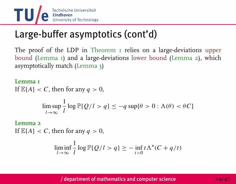
The proof of the LDP in Theorem 1 relies on a large-deviations upperbound (Lemma 1) and a large-deviations lower bound (Lemma 2), whichasymptotically match (Lemma 3)
Lemma 1If E{A} < C , then for any q > 0,
lim supl→∞
1l
logP{Q/ l > q} ≤ −q sup{θ > 0 : 3(θ) < θC}
Lemma 2If E{A} < C , then for any q > 0,
lim infl→∞
1l
logP{Q/ l > q} ≥ − inft>0
t3∗(C + q/t)

/ department of mathematics and computer science 25/47
Large-buffer asymptotics (cont’d)
Lemma 3If E{A} < C , then for any q > 0,
I (q) = inft>0
t3∗(C+q/t) = inft>0
supθ≥0{θ(q+Ct)−t3(θ)} = q sup{θ > 0 : 3(θ) < θC}
In the next slides we proceed to review the proofs of Lemmas 1 and 2
The proof of Lemma 3 is mostly technical and uses the convexity of thefunction 3(·)

/ department of mathematics and computer science 26/47
Large-buffer asymptotics (cont’d)
Proof of Lemma 1Using the supremum representation for Q,
P{Q > lq} = P{supt≥0{St−Ct} > lq} = P{∃t ≥ 0 : St−Ct > lq} ≤
∑t≥0
P{St−Ct > lq},
applying Chernoff’s bound, for any θ > 0,
≤
∑t≥0
e−θ(lq+Ct)et3(θ)= e−θlq
∑t≥0
(e3(θ)−Cθ
)t,
and restricting to θ for which 3(θ) < θC ,
≤ e−θlq 11− e3(θ)−Cθ
/ department of mathematics and computer science 27/47
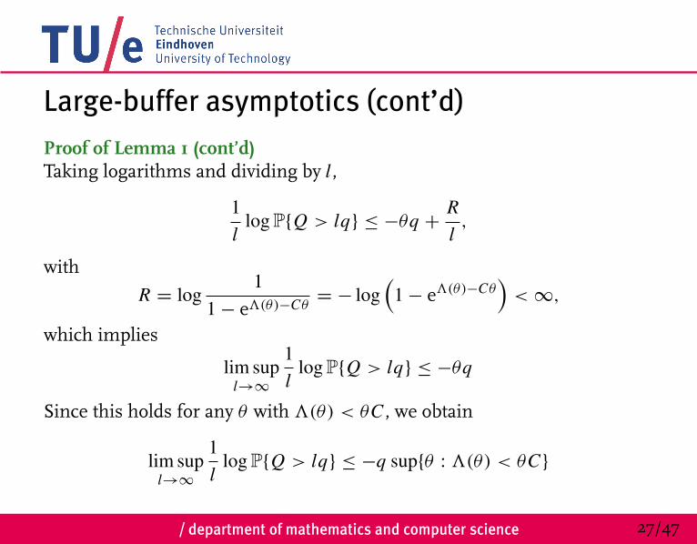
Large-buffer asymptotics (cont’d)
Proof of Lemma 1 (cont’d)Taking logarithms and dividing by l,
1l
logP{Q > lq} ≤ −θq +Rl,
with
R = log1
1− e3(θ)−Cθ = − log(
1− e3(θ)−Cθ)<∞,
which implies
lim supl→∞
1l
logP{Q > lq} ≤ −θq
Since this holds for any θ with 3(θ) < θC , we obtain
lim supl→∞
1l
logP{Q > lq} ≤ −q sup{θ : 3(θ) < θC}

/ department of mathematics and computer science 28/47
Large-buffer asymptotics (cont’d)
Proof of Lemma 2Using the supremum representation for Q,
P{Q > lq} = P{supt≥0{St−Ct} > lq} = P{∃t ≥ 0 : St−Ct > lq} ≥ P{Stl−Ctl > lq},
for any tl = 0, 1, . . .
Taking logarithms and dividing by l,
1l
logP{Q > lq} ≥1l
logP{Stl − Ctl > lq},
choosing tl = dlte, and noting that l ≤ dlte/t ,
≥tdlte
logP{Sdlte − Cdlte >dlte
tq} =
ttl
logP{Stl − Ctl >tlt
q}

/ department of mathematics and computer science 29/47
Large-buffer asymptotics (cont’d)
Proof of Lemma 2 (cont’d)Taking liminf’s,
lim infl→∞
1l
logP{Q > lq} ≥ lim infl→∞
ttl
logP{Stl − Ctl >tlt
q} =
lim inftl→∞
ttl
logP{Stl − Ctl >tlt
q} = t lim inftl→∞
1tl
logP{Stl > C + q/t},
and using the lower bound in Cramér’s theorem,
≥ −t3∗((C + q/t)+)
Since this holds for any t > 0, and3∗(·) is lower semi-continuous, it followsthat
lim infl→∞
1l
logP{Q > lq} ≥ − inft>0
t3∗((C+q/t)+) = − inft>0
t3∗((C+q/t)) = −I (q)

/ department of mathematics and computer science 30/47
Large-buffer asymptotics (cont’d)
Some observations based on the proof of Lemma 2:
• Note that a lower bound for 1l logP{Q > lq} is given by
1l
logP{Sdltqe − Cdltqe > lq} =dltqe
l1dltqe
logP{Sdltqedltqe
> C +lqdltqe}
• As l →∞, the latter lower bound behaves asymptotically as
tq1dltqe
logP{Sdltqedltqe
> C +qtq}
• Denoting tq = arg inft>0
t3∗(C + q/t), the latter expression converges to
−tq3∗(C + q/tq) = − inft>0
t3∗(C + q/t) = −I (q),
which coincides with behavior of 1l logP{Q > lq} stated in Theorem 1

/ department of mathematics and computer science 31/47
Large-buffer asymptotics (cont’d)
Some observations based on the proof of Lemma 2:
• Thus, the lower bound
P{Sdltqe − Cdltqe > lq}
for P{Q > lq} is asymptotically tight (on a logarithmic scale)
• In other words, the approximation
P{supt≥0{St − Ct} > lq} ≈ sup
t≥0P{St − Ct > lq}
is asymptotically exact (on a logarithmic scale)
• Also, tq = arg inft>0
t3∗(C + q/t) may be interpreted as the length of time
(normalized by l) during which the process (At)t∈Z exhibits an averagerate C + q/tq , and ltq corresponds to the most likely amount of time ittakes for the buffer content to reach level lq

/ department of mathematics and computer science 32/47
Many-sources asymptotics
So far we have focused on large-buffer asymptotics:the asymptotic buffer content distribution in a single-server queuefed by a single arrival stream where the buffer level grows large
We now turn the attention to many-sources asymptotics:the asymptotic buffer content distribution in a single-server queuefed by the superposition of several arrival streams where total number offlows grows large

/ department of mathematics and computer science 33/47
Many-sources asymptotics (cont’d)
Specifically, consider a single-server queue (switch in a communication net-work) with a time-slotted operation and a service capacity of NC customers(packets) per slot fed by N arrival streams (traffic sources)
Denote by A(i)t the amount of traffic generated by the i -th source in timeslot t
We assume that the sequence (A(i)t )t∈Z for each given i is stationary, but donot require that the amounts of traffic in successive slots are independent,thus allowing for temporal correlation, which is important in many applica-tions
We do assume that the sequences (A(i)t )t∈Z for different i ’s are i.i.d., withE{A(i)} < C for all i for stability

/ department of mathematics and computer science 34/47
Many-sources asymptotics (cont’d)
The stationary buffer content may be represented as
QN= sup
t≥0{SN
t − NCt},
where
• ANt =
∑Ni=1 A(i)t = A(1)t + · · · + A(N )t represents the aggregate amount
of traffic generated during slot t
• SNt =
∑t−1j=0 AN
− j = AN−t+1 + · · · + AN
0 represents the cumulative totalamount of traffic generated during slots −t + 1, . . . , 0

/ department of mathematics and computer science 35/47
Many-sources asymptotics (cont’d)
Define3t(θ) = logE{eθ S1
t }
as the log moment generating function of S1t , representing the cumulative
amount of traffic generated by a single source during slots −t + 1, . . . , 0
We do not require that the sequences (A(i)t )t∈Z for different i ’s are i.i.d., butif that does happen to hold, then
3t(θ) = logE{eθ S1t } = logE{eθ
∑t−1i=0 A1
−i } = logE{t−1∏i=0
eθ A1−i } =
logt−1∏i=0
E{eθ A1−i } = log
(E{eθ A
}
)t= t logE{eθ A
} = t logE{eθ S11}

/ department of mathematics and computer science 36/47
Many-sources asymptotics (cont’d)
We make two assumptions
• Assumption 1 3t(θ) is finite in a neighborhood of θ around 0, for all t
• Assumption 2 limt→∞1t3t(θ) exists, is finite, and differentiable in a
neighborhood of θ around 0
As before, denote by
3∗t (x) = supθ∈R{θx −3t(θ)}
the convex conjugate of 3t(·)
For any q > 0, define the rate function
I (q) = inft∈N
3∗t (q + Ct)

/ department of mathematics and computer science 37/47
Many-sources asymptotics (cont’d)
Theorem 2Under the stability condition E{A(i)} < C and Assumptions 1 and 2, for anyq > 0,
−I (q+) ≤ lim infN→∞
1N
logP{QN > Nq}
≤ lim supN→∞
1N
logP{QN > Nq} ≤ −I (q)
If 3∗t (·) is continuous for each t , then Theorem 2 yields
limN→∞
1N
logP{QN > Nq} = −I (q)
/ department of mathematics and computer science 38/47
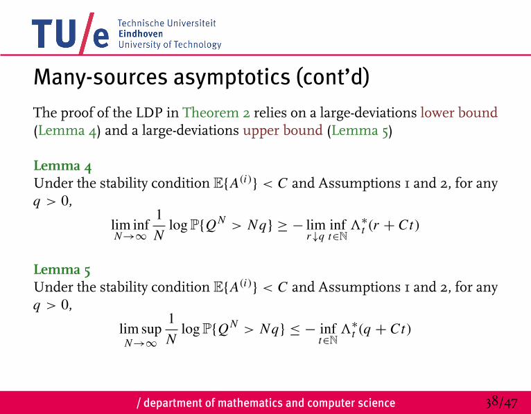
Many-sources asymptotics (cont’d)
The proof of the LDP in Theorem 2 relies on a large-deviations lower bound(Lemma 4) and a large-deviations upper bound (Lemma 5)
Lemma 4Under the stability condition E{A(i)} < C and Assumptions 1 and 2, for anyq > 0,
lim infN→∞
1N
logP{QN > Nq} ≥ − limr↓q
inft∈N
3∗t (r + Ct)
Lemma 5Under the stability condition E{A(i)} < C and Assumptions 1 and 2, for anyq > 0,
lim supN→∞
1N
logP{QN > Nq} ≤ − inft∈N
3∗t (q + Ct)

/ department of mathematics and computer science 39/47
Many-sources asymptotics (cont’d)
Proof of Lemma 4The proof is somewhat similar in spirit to that of Lemma 2
Using the supremum representation for Q,
P{QN > Nq} = P{supt≥0{SN
t − NCt} > Nq} = P{∃t ≥ 0 : SNt − NCt > Nq}
≥ P{SNt /N > q + Ct} = P{SN
t > Nq + NCt}
for any fixed t ∈ N
Taking logarithms and dividing by N ,
1N
logP{QN > Nq} ≥1N
logP{SNt /N > q + Ct}

/ department of mathematics and computer science 40/47
Many-sources asymptotics (cont’d)
Proof of Lemma 4 (cont’d)Taking liminf’s and applying the lower bound in Cramér’s theorem,
lim infN→∞
1N
logP{QN > Nq} ≥ −3∗t ((q + Ct)+)
Since this holds for any t ∈ N, and using the properties of the function3∗t (·),
≥ − inft∈N
infr>q
3∗t (r + Ct) = − infr>q
inft∈N
3∗t (r + Ct) = − limr↓q
inft∈N
3∗t (r + Ct)

/ department of mathematics and computer science 41/47
Many-sources asymptotics (cont’d)
Proof of Lemma 5The proof proceeds in a somewhat similar vein as that of Lemma 1
Using the supremum representation for Q, for any given t0,
P{QN > Nq} = P{supt≥0{SN
t − NCt} > Nq}
= P{∃t ≥ 0 : SNt − NCt > Nq}
≤
∑t≥0
P{SNt /N > q + Ct}
=
t0∑t=0
P{SNt /N > q + Ct} +
∑t>t0
P{SNt /N > q + Ct}

/ department of mathematics and computer science 42/47
Many-sources asymptotics (cont’d)
Proof of Lemma 5 (cont’d)Taking logarithms, dividing by N , taking limsup’s, and using the ‘principleof the largest term’,
lim supN→∞
1N
logP{QN > Nq}
≤ lim supN→∞
1N
log
( t0∑t=0
P{SNt /N > q + Ct} +
∑t>t0
P{SNt /N > q + Ct}
)
≤ max0≤t≤t0
lim supN→∞
1N
logP{SNt /N > q + Ct}
∨ lim supN→∞
1N
log∑t>t0
P{SNt /N > q + Ct}

/ department of mathematics and computer science 43/47
Many-sources asymptotics (cont’d)
Proof of Lemma 5 (cont’d)Applying the upper bound in Cramér’s theorem, for any given t ,
lim supN→∞
1N
logP{SNt /N > q + Ct} ≤ −3∗t (q + Ct)
It may further be shown that
lim supN→∞
1N
log∑t>t0
P{SNt /N > q + Ct} → −∞
as t0→∞
Combining these two facts, the statement of the lemma follows

/ department of mathematics and computer science 44/47
Many-sources asymptotics (cont’d)
Some observations based on the proof of Lemma 5:
• Note that a lower bound for 1N logP{QN > Nq} is given by
1N
logP{SNtq /N − Ctq > q} =
1N
logP{SNtq /N > q + Ctq}
• Denoting tq = arg inft∈N
3∗t (q + Ct), the latter lower bound converges to
3∗tq(q + Ctq) = inft∈N
3∗t (q + Ct),
which coincides with behavior of 1N logP{QN > Nq} stated in Theo-
rem 2

/ department of mathematics and computer science 45/47
Many-sources asymptotics (cont’d)
Some observations based on the proof of Lemma 5:
• Thus, the lower bound
P{SNtq /N − Ctq > q}
for P{QN > Nq} is asymptotically tight (on a logarithmic scale)
• In other words, the approximation
P{supt≥0{SN
t − C Nt} > Nq} ≈ supt≥0
P{SNt − C Nt > Nq}
is asymptotically exact (on a logarithmic scale)
• Also, tq may be interpreted as the most likely time it takes for the buffercontent to reach level Nq

/ department of mathematics and computer science 46/47
Bibliography
V.E. Benes (1963). General Stochastic Processes in the Theory of Queues.Addison-Wesley.D.D. Botvich, N.G. Duffield (1995). Large deviations, economies of scale,and the shape of the loss curve in large multiplexers. Queueing Systems 20,293–320.C. Courcoubetis, R.R. Weber (1996). Buffer overflow asymptotics for abuffer handling many traffic resources. J. Appl. Prob. 33, 886–903.A. Dembo, O. Zeitouni (1998). Large Deviations Techniques and Applications.Springer, Berlin.A. Ganesh, N. O’Connell, D. Wischik (2004). Big Queues. Springer, Berlin.P.W. Glynn, W. Whitt (1994). Logarithmic asymptotics for steady-state tailprobabilities in a single-server queue. J. Appl. Prob. 31A, 131–156.R.M. Loynes (1962). The stability of a queue with non-independent interar-rival and service times. Proc. Cambridge Phil. Soc. 58.

/ department of mathematics and computer science 47/47
Bibliography (cont’d)
A. Shwartz, A. Weiss (1995). Large Deviations for Performance Analysis. Chap-man & Hall.A. Simonian, J. Guibert (1995). Large deviations approximations for fluidqueues fed by a large number of on/off sources. J. Sel. Areas Commun 13 (6),1017–1027.A. Weiss (1986). A new technique for analyzing large traffic systems. Adv.Appl. Prob. 18, 506–532.