1

LIVE MESH: AN INTERACTIVE 3D IMAGE

SEGMENTATION TOOL

John Edwards, Parris Egbert, Bryan Morse

Abstract—Image segmentation is the process by which objects are extracted from their surroundings in

images. Segmentation in two dimensional images is a well-researched area, with both user-interactive and

non-user-interactive tools to perform this function. While research has been done in three-dimensional

image segmentation, few user-interactive tools exist that work directly in 3D. We present Live Mesh, an

algorithm that provides a highly user-interactive environment for effective 3D image segmentation. It

expands on the concepts of Live Wire, and uses a three-dimensional implementation of the powerful

Dijkstra’s algorithm. The Live Mesh algorithm allows the user to effectively drag mesh patches, or

surfaces over a 3D object. SimpleSeg is an implementation of Live Mesh that shows the utility and

effectiveness of the Live Mesh method.

Index Terms—Segmentation, edge and feature detection, image processing software.

1 Introduction

Three-dimensional object segmentation refers to the task of detecting and describing

objects in volume data. Applications such as medical imaging, geological surveying, and

computational fluid dynamics can all benefit greatly from 3D image segmentation. This

paper outlines Live Mesh, a novel, interactive 3D image segmentation algorithm.

Many interactive 3D object segmentation strategies are based on 2D techniques

such as Snakes [12] or Live Wire [1,2] (also known as Intelligent Scissors). After

segmenting in 2D, the descriptions are combined and interpolated to produce a 3D object.

While simple to use, these approaches don’t allow the user to work on the data as a

whole. Rather, they present the user with one slice at a time. The tools and user may

make errors because of lack of context of the slice data. The Live Mesh algorithm works

on the volume data, and, in addition, allows the user to interact in a 3D environment.

The Live Mesh method is a 3D extension of Live Wire, an algorithm that uses

Dijkstra’s shortest-cost algorithm and a user-interactive interface to find object edges.

Live Wire has proven to be very powerful and is widely used because of its high degree

of user-interactivity. This is because automatic segmentation is still an unsolved problem

2

and many datasets still require expert knowledge from users. Live Mesh retains the user-

interactivity of Live Wire while extending the working space to three dimensions.

Novel ideas proposed herein include a 3D extension of the Live Wire cost

function, a spatial restriction for the 3D graph search and the Live Mesh algorithm. A

simple implementation of the Live Mesh method, the SimpleSeg application, is also

briefly discussed.

2 Previous Work

Live Wire stands out among the class of user-interactive image segmentation

tools. The user clicks on an edge of the object with the mouse, defining a “seed point”.

The user then moves the cursor to some other portion of the object’s edge. The pixel that

lies under the cursor is called the “free point”. As the free point moves, a wire

connecting the seed point and the free point automatically snaps to the edge. While the

algorithm does do significant automatic segmentation (by snapping to the edge), the user

maintains complete control in that he or she can adjust the location of the free pixel if the

algorithm fails to find the correct boundary.

There are many different methods of extending Live Wire to 3D, though most of

them use 2D Live Wire on successive slices. Schenk et al. [5] have optimized this

process by only computing the cost for successive slices on regions that fall within a

given distance from a reference slice’s completed boundary. A distance map, showing

distances from the reference slice’s boundary, is generated using a chamfering process.

This distance map is used to determine which pixels in the current slice will be used for

the local cost computation. In addition to speeding cost computation, local cost feature

optimization can be performed.

Schenk et al. also introduce an automatic segmentation step using shape-based

interpolation followed by a Live Wire-driven optimization process [5,7]. The user

segments selected slices, then intermediate slices are automatically interpolated.

Falcao and Udupa [6] developed a method that determines object boundary

information from orthogonal slices of a volume segmented by a user. This technique

3

allows the user to segment a minimal number of slices, reducing the total segmentation

time.

König and Hesser’s method [9] allows the user to select three seed points. After

selection, Live Wire is used to generate an initial frame and then “spokes.” After the

spokes are found, a gap filling algorithm is used to close the space between spokes.

The above 3D segmentation methods have steps in which automatic segmentation

is done that can’t be controlled by the user in real-time. Additionally, the entire

segmentation is done in disjoint steps. Live Mesh overcomes these weaknesses by

providing the user with a single interface and a single technique so that the user can

perform the entire segmentation using one continuous method. Live Mesh also avoids

automatic segmentation, thereby keeping the user in control of the algorithm at all times,

just as 2D Live Wire allows real-time user control.

3 Graph Search

Live Mesh is used much like Live Wire. A mesh of wires snaps to the object

boundary as the user drags the cursor over the surface of an object. Each wire in the

mesh is the shortest-cost path from the current location of the cursor (free point) back to

the location where the user initiated the mesh (seed point). The dynamic nature of Live

Wire and Live Mesh (i.e., the wires snapping to the boundary immediately upon

movement of the cursor) is possible through use of Dijkstra’s algorithm.

Graph searching in three dimensions requires a 3D version of the cost function

(Section 3.1). In addition, since Live Mesh is a user-interactive tool, we have developed

optimizations (Section 3.2) so that the algorithm is fast enough to keep the software

responsive to the user.

3.1 Cost function

The cost function used in Dijkstra’s algorithm is formulated such that the cost is

lowest along edges of an object, ensuring that the lowest cost path will lie along a

boundary. Three primary image features are used: Laplacian zero-crossing ( Zf ), gradient

magnitude ( Gf ) and gradient direction ( Df ). Each feature is weighted with constants

( Z , G and D ). The cost function (as formulated by Mortensen and Barrett [1,2]) is

4

),()()(),(cost vufvfvfvu DDGGZZ ++= . (1)

The Laplacian zero-crossing feature gives an indication of whether a pixel is on

an edge or not. The Laplacian operator sums the second derivatives of the image

intensity in the axis directions. We consider zero or zero crossing pixels to be an

inflection point in the intensity. The Laplacian image is binarized such that all pixels on

zero crossings are given a pixel value of zero and all other pixels are given a value of

one. )(vf Z is defined as the value of pixel v in the Laplacian image. Since this value

will be zero or one, the contribution the Laplacian makes to the cost function (Equation 1)

will be either zero or Z .

The gradient magnitude feature of the cost function gives us an idea of how

confident we are that this voxel is an edge (as opposed as “whether the voxel is an edge

or not,” which is given us by the Laplacian zero-crossing calculation). Voxels with a

high gradient magnitude have a high likelihood of being edges. The final cost of a voxel

near an edge should be low, so )(vfG is computed using the inverse of the gradient:

)max()(1

)max()()max()(

GvG

GvGGvfG =

= (2)

where )max(G is the maximum gradient magnitude value of any voxel in the image.

Therefore Gf is the inverse of the normalized gradient magnitude at voxel v.

The gradient direction feature is defined as follows: let p and q be two voxels in a

3D image. A normalized gradient direction vector )( pD is defined by the partial

derivatives xI , yI and zI and by definition points up the steepest slope at that point. We

first define L as the vector orthogonal to )( pq such that the difference between L and

)( pD is minimized:

)(),()(),(),(pqqpTpqqpTqpL

= (3)

where

)()(),( pqpDqpT = . (4)

),( qpT is the vector orthogonal to both )( pD and )( pq (Figure 1b). By taking the

cross product of ),( qpT and )( pq we find L , which is the vector orthogonal to

5

)( pq that is closest to )( pD (Figure 1c). We can also think of L as being a vector

orthogonal to )( pq that is in the plane containing both )( pq and )( pD .

At this point we define angles ),( qpd p and ),( qpdq :

( )( ))(),(cos),(

),()(cos),(1

1

qDqpLqpd

qpLpDqpd

q

p

=

=

. (5)

Df is then defined as the sum of these angles:

( )),(),(32),( qpdqpdqpf qpD +=

(6)

32 is used to normalize Df to a value of one. L is defined such that it is no

more than 2 different from )( pD (Equation 5), so ),( qpd p has a maximum value of

2 . ),( qpdq can have a maximum value of . Thus the normalization factor is

3

2

2

1=

+.

(a) (b) (c)

Figure 1 Calculation of L(a) Starting vectors )( pq and )( pD . (b) ),( qpT is a vector orthogonal to both )( pq and

)( pD . (c) L is orthogonal to )( pq and ),( qpT .

3.2 Search optimization

One challenge in extending Live Wire to three dimensions is the actual

computation time of the graph search. The computational complexity of the search is

increased by an order of magnitude when adding another dimension, which renders a

6

traditional Dijkstra search very expensive. We have developed a new method of

restricting the search space.

By default, the graph search expands throughout the entire image while the user is

usually interested in only a portion of the image. The time required for the graph search

to find the shortest cost path from the free point to the seed point can be decreased by

restricting the graph search to voxels in the neighborhood of the free and seed points

(Figure 2a). We define the search space as all voxels within x voxels of the line between

the seed and free points, where x is a user-specified value.

If a restriction is used, the path is optimal only within the search space. This is

fine if the edge contour is relatively linear, but if the image edges are poorly defined or

jagged, then the locally optimum path may in fact be very far from the globally optimum

path. An additional problem is that once the free point is moved outside of the restricted

search space the search must be restarted. The following two sections address these

difficulties.

3.2.1.1 Expanded Search Space

Suppose a restricted search has run to completion and each point in the search

space has a locally optimal path back to the seed point. If both the seed and free points

are still in place, then a new, expanded search can be started to find a path that is optimal

within a larger search area. A naive implementation might be to simply re-search all

points in the new, larger search area. However, many of the points in the original search

likely have globally optimal paths already. For example, every neighbor of the seed point

is guaranteed to have a globally optimal path even in a restricted search.

Our algorithm takes advantage of the fact that we already have some globally

optimal information. The original search area is re-searched from the outside-in only as

far as needed. We use Dijkstra’s algorithm with a few modifications, as follows:

7

Algorithm 1 Expanded Restricted SearchDescription: Finds shortest cost path from every Vertex v backto a seed Vertex s.Structure: Vertex containing three properties:

Vertex prevNumber costBoolean isVisited

Input: seed vertex s, graph G, SortedList q, Set restrictionOutput: prev pointer for each vertex v in G, list r suitable forexpanded active list

(1) SortedList q r (2) Vertex v (3) Number c (4) for every Vertex v in G (5) if q is empty (6) set v.cost = INFINITY (7) end if (8) set v.isVisited = false (9) end for (10) set s.cost = 0 (11) insert s into q (12) while q is not empty (13) set v = least cost Vertex in q (14) remove v from q (15) set v.isVisited = true (16) for each neighbor Vertex vi near v (17) if not vi.isVisited (18) if restriction does not contain vi (19) insert v into r (20) else (21) set c = cost(v, vi) (22) if v.cost + c < vi.cost (23) set vi.cost = v.cost + c (24) set vi.prev = v (25) insert vi into q (26) end if (27) end if (28) end if (29) end for (30) end while

The active list q contains all voxels that have a non-infinite cost and that have not yet

been visited. q is passed into the algorithm as input rather than being created inside the

algorithm, as it is in the original Dijkstra’s algorithm. Every vertex is given a value of

infinity on only the first search.

In the above algorithm, any vertex in the search space that has a neighbor vertex that

is outside of the search space is added to a cost-sorted list r (line 19). At the conclusion

8

of the algorithm, r contains all vertices along the boundary of the restriction. r can then

be used as the active list in a subsequent, expanded search (Figures 11 and 12).

(a) (b) (c)

(d) (e) (f)

Figure 2 Expanded search(a) Setting up the initial graph search. (b) Search in progress. Searched area is shaded. (c) Completion ofinitial graph search. (d) Setting up the expanded graph search. (e) Completion of expanded graph search.(f) _ is the area re-searched.

Each vertex in the graph must be reset to “not-visited” (line 8) in case vertices

inside the old restriction need to be re-searched. Any vertex inside the old boundary that

does not have an optimal path within the new boundary will be visited again in the new

search. The area inside the previous search that is re-searched is called _, and ideally it

should be very small. In some cases, however, it is large, even as large as the previous

search space itself. In these cases the restricted search is extremely inefficient, as the

previous search space is entirely re-searched the second time.

While improved, the new path found after an expanded search is still not globally

optimal, unless the path from the v to s is shorter than the path from each point on the

search boundary back to s.

9

(a) (b) (c) (d)

(e) (f) (g) (h)

Figure 3 Expanded Search ExampleThe active list q is in red while the sorted list r is in yellow. (a) Beginning the initial search. (b) After theinitial search has completed. (c) The new search with active list initialized to be r from the previous search.(d-h) Continuing on through the first and second expanded searches.

3.2.1.2 Changed Search Space

Suppose a restricted search is running and the free point is suddenly moved

outside of the search space. A new search must be started, ideally using information

obtained in the aborted search. This can be accomplished using exactly the same

algorithm as the expanded search (Algorithm 1). The only difference is that, after the

free point is moved and the current search is aborted, r and the active list q must be

combined to form the new active list before restarting the algorithm (Figures 4 and 5).

The area _ tends to be somewhat larger for a changed search compared to an

expanded search. However, in practice, users tend not to move the free point (e.g.,

mouse cursor) much at all until at least an initial wire appears. At that time, if the free

point is moved at all, it is usually moved either closer or further from the seed point, not

in a different direction from it. If it is simply moved closer, the free point usually

remains within the search space and an expanded search can take place. If it is moved

further away, _ tends to be small as the new search space is close to, and often is a

superset of, the old search space.

10

(a) (b)

(c) (d) (e)

Figure 4 Changed search(a) Setting up the initial graph search. (b) Search in progress. Searched area is shaded. (c) After the

free point is moved the changed search is set up. The new active list is the union of r and theactive list q. (d) Completed changed search. (e) Area _ of initial search that had to be re-searched.

11

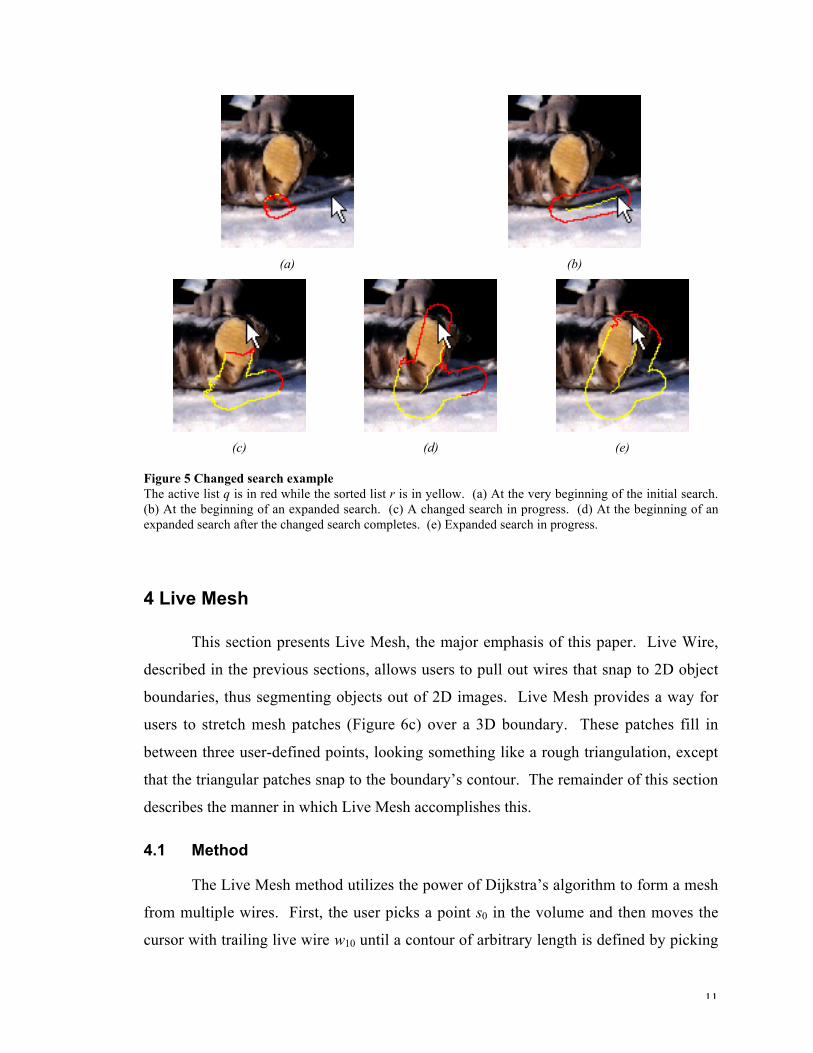
(a) (b)

(c) (d) (e)

Figure 5 Changed search exampleThe active list q is in red while the sorted list r is in yellow. (a) At the very beginning of the initial search.(b) At the beginning of an expanded search. (c) A changed search in progress. (d) At the beginning of anexpanded search after the changed search completes. (e) Expanded search in progress.

4 Live Mesh

This section presents Live Mesh, the major emphasis of this paper. Live Wire,

described in the previous sections, allows users to pull out wires that snap to 2D object

boundaries, thus segmenting objects out of 2D images. Live Mesh provides a way for

users to stretch mesh patches (Figure 6c) over a 3D boundary. These patches fill in

between three user-defined points, looking something like a rough triangulation, except

that the triangular patches snap to the boundary’s contour. The remainder of this section

describes the manner in which Live Mesh accomplishes this.

4.1 Method

The Live Mesh method utilizes the power of Dijkstra’s algorithm to form a mesh

from multiple wires. First, the user picks a point s0 in the volume and then moves the

cursor with trailing live wire w10 until a contour of arbitrary length is defined by picking

12

the ending point s1 (Figure 6a). While defining this wire, the graph search is not only

finding the shortest-cost path from s1 to the seed point s0, but also finds the shortest-cost

path from every voxel within the search space (ideally defined by the entire image, but

possibly bounded by a restriction). That is, after the graph search completes we are left

with shortest-cost paths reaching back from each voxel in the search space to s0.

After picking s1, the user moves the cursor to define the next wire w21. A new

graph search is started with s1 as the seed voxel and wire w21 is displayed in real-time

(Figure 6b). As mentioned, Dijkstra’s algorithm has already found shortest-cost paths

from voxels surrounding the original seed point s0, and so, with no additional path

searching, we can display shortest-cost paths leading to s0 from every voxel defining wire

w21 (Figure 6c).

Once point s2 has been chosen, thereby fixing the mesh s0 s1 s2, the user moves the

cursor and a new mesh drags out, using graph searches that have already been completed

or are well in progress. If the free point s3 is close to s1 then the new mesh is defined as

shortest-cost paths from every point in w32 back to s1 (Figure 6e). If s3 is closer to s0 than

s1, the new mesh is made of paths from w32 back to s0 (Figure 6h). s0 and s1 both work

equally as well as seed points for a wire mesh as they both have expanded their

wavefronts during the definitions of w10 and w21, respectively. The user selects s3 which

completes the second patch using s1 and s2, or s0 and s2.

The user continues defining meshes in this way until the surface is covered. The

fact that little or no extra graph searching needs to occur to define the extra wires forming

the mesh makes this algorithm very powerful. Once the graph search out from s0 has

been completed, any two points s1 and s2 in the entire image can compute a wire w21, and

every point in w21 will immediately have a shortest-cost path back to s0.

13

(a) (b) (c)

(d) (e) (f)

(g) (h) (i)

Figure 6 Live Mesh Diagram(a) Initial Live Wire with so as the seed and s1 as the free point. (b) s2 is the new free point. (c) Shortest-cost paths to s0 have already been computed so a mesh is formed from w21 to s 0 with only minimaloverhead. (d-f) A new mesh from w32 to s1. (g-i) Free point s3 was moved from its previous position andnew mesh goes back to s0 rather than s1 since the new free point is now closer to s0.

The end result, once the user has covered the object in meshes, is a set of points

that lie on the object boundary. The points are generally very dense; along the wires of

the mesh they are contiguous. Exactly how an object is segmented using these points is

application-specific. The application may simply use the points as a set, or it may use

14

topological information found in the individual wires (e.g. )10,58,102( is linked to

)10,58,101( which is linked to )11,57,100( ...).

5 The SimpleSeg Application

The previous sections discuss the Live Mesh algorithm and its powerful features.

This section describes SimpleSeg, an application implementing the Live Mesh algorithm.

We first describe the visualization and picking techniques of SimpleSeg. Following that

discussion we provide the results of a small user study conducted using SimpleSeg.

5.1 Data Visualization

Since Live Mesh deals with data in three dimensions, a way for the user to

interact with the data in three dimensions is needed. SimpleSeg provides four different

views of the data (Figure 7a): a volume-rendered view and three orthogonal 2D slices of

the volume. These 2D slices are present to allow the user to visualize and pick obscured

data. This has no effect on the underlying Live Mesh algorithm, which still searches in

3D, regardless of which views are used to visualize the data.

5.2 Mesh Visualization

As the user creates a new mesh, each wire in the mesh is displayed in red. Once

the user finishes a mesh, the wires are displayed in blue and the new, current mesh is

displayed in red. This is shown in Figure 8.

A surface can be generated from finished meshes dynamically. It has been

observed that turning on the surface display has been very helpful to users in visualizing

the mesh.

The mesh is displayed in the volume rendered window. This way the user can

observe the entire mesh being constructed while the user works. Even while the user

works on the 2D slices the mesh can be seen in 3D (Figure 7). If the object is obscured,

then the rendering of the volume itself can be turned off and the mesh displayed alone.

This is assistive especially if the user has some a priori idea of what the object looks like.

15

(a) (b) (c)

Figure 7 Mesh visualization while working in 2D(a) View of entire application. (b) Close-up view of the upper-left window in which the user is currentlyworking. (c) Close-up view of the lower-left window (volume rendered) where the user observes the meshbeing constructed.

(a) (b) (c)

(d) (e) (f)

Figure 8 Mesh Visualization(a) Dragging out an initial mesh. (b-c) Finished meshes displayed in blue; active mesh in red. (d-f) Withsurface display turned on. (e) In the user’s hurry he failed to notice certain holes (which were visible onlyfrom certain angles). (f) After completing the segmentation and closing holes.

16

5.3 Testing Results

We tried out the SimpleSeg application on a few users to find out how accurate,

reproducible and fast the Live Mesh algorithm is in the SimpleSeg implementation

compared to traditional Live Wire. We found that accuracy was about two orders of

magnitude better with Live Mesh on a dataset containing only a sphere. We measured

repeatability and segmentation time using more complex datasets, including one (the

caudate nucleus of the human brain) in which the data was obscured in the 3D view, so

the users had to work exclusively in the 2D view of SimpleSeg. Live Wire performed

better than SimpleSeg in both repeatability and segmentation time. We observed that the

users learned Live Wire more quickly than Live Mesh, largely due to the fact that they

had difficulty navigating and interacting in the three-dimensional SimpleSeg interface. A

more complete study would test using both novice and experienced SimpleSeg users

using more complex datasets.

6 Conclusions and Future Work

Live Mesh is a powerful 3D image segmentation tool, and has great possibilities

for the future. The 3D cost function extension is effective for finding object edges. The

restricted search and pre-processing of the cost function make the algorithm fast enough

to be responsive to the user. The Live Mesh algorithm, including the idea of pulling

patchwork meshes over 3D object boundaries, is an intuitive extension to the Live Wire

method.

Preliminary results from using SimpleSeg show that points composing the meshes

tend to be on or very close to the desired object boundary for simple datasets, though the

repeatability of such needs further study. The Live Mesh algorithm provides a solid

foundation for highly repeatable segmentations, but to get a more meaningful

repeatability measure the segmentation needs a gap-filling post-processing step, such as

is presented in [9].

Live Mesh could be improved by modifications suggested for Live Wire such as

using user motions to restrict the search space [3,4] and pre-processing steps to reduce

the size of the search graph [9,10]. The gradient direction element of the cost function is

highly sensitive to noise, and Mortensen and Barrett [8] removed it altogether, preferring

17

a tobogganing pre-processing step. Haenselmann and Effelsberg [11] use a wavelet-

based cost function to account for weaker edges and even for instances where there is no

clearly recognizable edge.

18

19

References 1 E. N. Mortensen and W. A. Barrett, “Intelligent scissors for image composition,” in SIGGRAPH95 Conference Proceedings, R. Cook, ed., Annual Conference Series, pp. 191-198, ACMSIGGRAPH, Addison Wesley, Aug. 1995. held in Los Angeles, California, 06-11 August 1995.

2 E. N. Mortensen and W. A. Barrett, “Interactive Segmentation with Intelligent Scissors,”Graphical Models and Image Processing 60, pp. 349-384, 1998.

3 A.X. Falcao, J.K. Udupa, S. Samarasekera, S. Sharma, B.E. Hirsch, and R.A. Lotufo, “User-steered image segmentation paradigms: live-wire and live-lane,” Graphical Models and ImageProcessing. vol. 60. no. 4. pp. 233-260, Jul, 1998.

4 A.X. Falcao, J.K. Udupa, S. Samarasekera, and F.K. Miyazawa, “An ultra-fast user-steeredimage segmentation paradigm: live-wire-on-the-fly,” Proceedings of SPIE on Medical Imaging.San Diego, CA, vol. 3661, pp. 184-191, Feb, 1999.

5 A. Schenk, G. Prause, and H.O. Peitgen, “Local Cost Computation for Efficient Segmentationof 3D Objects with Live Wire,” Proceedings of SPIE on Medical Imaging. vol. 4322, pp. 1357-1363, 2001.

6 A.X. Falcao, and J.K. Udupa, “Segmentation of 3D Objects using Live Wire,” Proceedings ofSPIE on Medical Imaging. vol. 3034, pp. 228-235, 1997.

7 A. Schenk, G. Prause, H.-O. Peitgen, “Efficient Semiautomatic Segmentation of 3D Objects inMedical Images,” Medical Image Computing and Computer-Assisted Intervention, MICCAI. pp.186-195, Oct, 2000.

8 E. N. Mortensen, W. A. Barrett, “Toboggan-Based Intelligent Scissors with a Four ParameterEdge Model,” IEEE: Computer Vision and Pattern Recognition. 2, pp. 452-458, 1999.

9 S. König, J. Hesser, “3D Live-Wires on Pre-Segmented Volume Data,” Proc. Of SPIE.vol.5747, 2005.

10 K. C. H. Wong, P. A. Heng, T. T. Wong, “Accelerating Intelligent Scissors Using SlimmedGraphs,” Journal of Graphic Tools. 5(2), pp. 1-13, 2000.

11 T. Haenselmann, W. Effelsberg, “Wavelet Based Semi-AutomaticLive-Wire Segmentation,” SPIE Human Vision and Electronic Imaging VII. vol. 4662, pp. 260-269, 2003.

12 M. Kass, A. Witkin, and D. Terzopoulos, “Snakes: Active contour models,” InternationalJournal of Computer Vision 1(4), pp. 321-331, 1988.