LIVE LOAD TESTING AND ANALYSIS OF THE SOUTHBOUND

SPAN OF U.S. ROUTE 15 OVER INTERSTATE-66

William Norfleet Collins

Thesis submitted to the Faculty of the Virginia Polytechnic Institute and State University

in partial fulfillment of the requirements for the degree of

Master of Science In

Civil Engineering

Thomas E. Cousins, Chair

Carin L. Roberts-Wollmann

Elisa D. Sotelino

July 30, 2010

Blacksburg, Virginia

Keywords: Live Load Test, Federal Highway Administration (FHWA), Long-Term Bridge Performance (LTBP) Program, wheel load distribution, dynamic load allowance, neutral axis, bridge bearings, expansion joints

LIVE LOAD TESTING AND ANALYSIS OF THE SOUTHBOUND

SPAN OF U.S. ROUTE 15 OVER INTERSTATE-66

William Norfleet Collins

(ABSTRACT)

As aging bridges around the United States begin to near the end of their service lives,

more funding must be allocated for their rehabilitation or replacement. The Federal Highway

Administration’s (FHWA) Long-Term Bridge Performance (LTBP) Program has been developed

to help bridge stakeholders make the best decisions concerning the allocation of these funds.

This is done through the use of high quality data obtained through numerous testing processes.

As part of the LTBP Pilot Program, researchers have performed live load tests on the

U.S. Route 15 Southbound bridge over Interstate-66. The main performance and behavior

characteristics focused on are service strain and deflection, wheel load distribution, dynamic load

allowance, and rotational behavior of bridge bearings.

Data from this test will be used as a tool in developing and refining a plan for long-term

bridge monitoring. This includes identifying the primarily loaded girders and their expected

range of response under ambient traffic conditions. Information obtained from this test will also

aid in the refinement of finite element models by offering insight into the performance of

individual bridge components, as well as overall global behavior. Finally, the methods and

results of this test have been documented to allow for comparison with future testing of this

bridge, which will yield information concerning the changes in bridge behavior over time.

iii

Acknowledgements

I would like to extend my deepest gratitude to everyone who has helped and supported

me throughout this research. To my committee members, Dr. Tommy Cousins, Dr. Carin

Roberts-Wollmann, and Dr. Elisa Sotelino, I offer thanks for your experience, guidance, and

patience. It has been a pleasure working for all of you, and I hope that you have enjoyed it as

much as I have. The hard work of Ben Dymond, Jon Emenheiser, Brett Farmer, Marc Maguire,

Brian Pailes, and Brenton Stone is much appreciated. Without the stellar effort of these men on

site this research would have never taken place. Thanks to Amey Bapat for developing

analytical models of the bridge, and Dennis Huffmann for building instrumentation jigs. Thanks

to everyone else at VTRC and the rest of the LTBP team who have helped with this research

along the way. Words cannot express the gratitude I have for the love and support of my parents

and family, not only throughout this process but for my entire life. I would not be who I am

today without you. To my son Liam I offer thanks for being my biggest source of motivation

and procrastination at the same time. I can’t think of a better excuse to take a break from work.

Lastly, I would like to thank my wife, Kate Collins, for her love and support throughout this

process. Thank you for letting me become a student again, and for being my Sugar Mamma. It’s

been a blast and I think we should do it all over again.

iv

TABLE OF CONTENTS

Chapter 1: Introduction .......................................................................................................1 1.1 Long-Term Bridge Performance Program ........................................................................1 1.2 Virginia Pilot Bridge .......................................................................................................2

1.3 Scope and Objectives of This Study .................................................................................8 1.4 Thesis Organization ....................................................................................................... 10

Chapter 2: Literature Review ............................................................................................ 11 2.1 Live Load Testing.......................................................................................................... 11

2.1.1 Bridge Characterization ......................................................................................... 11 2.1.2 Loading Application .............................................................................................. 12

2.1.3 Data Collection ...................................................................................................... 13 2.2 Distribution Factors ....................................................................................................... 15

2.2.1 AASHTO Live Load Distribution Equations .......................................................... 15 2.2.2 Experimental Calculation of Distribution Factors ................................................... 19

2.3 Dynamic Load Allowance ............................................................................................. 20 2.3.1 AASHTO Dynamic Load Allowance ..................................................................... 23

2.3.2 Experimental Calculation of Dynamic Load Allowance ......................................... 23 2.4 Bearing Rotation Behavior ............................................................................................ 24

2.5 Composite Action .......................................................................................................... 25 2.6 Literature Review Summary .......................................................................................... 26

Chapter 3: Experimental Procedure .................................................................................. 27 3.1 Desired Data .................................................................................................................. 27

3.2 Bridge Instrumentation .................................................................................................. 27 3.2.1 Strain Transducers ................................................................................................. 28

3.2.2 Deflectometers ....................................................................................................... 32 3.2.3 Inclinometers and Tiltmeters .................................................................................. 34

3.2.4 Linear Variable Differential Transformers ............................................................. 36 3.2.5 Thermocouples and Thermometers ........................................................................ 38

3.2.6 Truck Locating Marker .......................................................................................... 38 3.2.7 Instrumentation Layout .......................................................................................... 39

3.3 Data Acquisition ............................................................................................................ 40 3.4 Instrument Calibration ................................................................................................... 41

3.5 Loading Procedure......................................................................................................... 42 3.5.1 Truck Description .................................................................................................. 42

3.5.2 Travel Orientations ................................................................................................ 43 3.5.3 Loading Speeds...................................................................................................... 44

3.6 Data Organization .......................................................................................................... 46 3.7 Data Reporting .............................................................................................................. 49

Chapter 4: Experimental Results ....................................................................................... 50 4.1 Service Strain and Deflection Results at Four Tenths of Span Length ............................ 50

4.1.1 Service Strain Results ............................................................................................ 50 4.1.2 Comparison of Strain Results Between North and South Spans .............................. 55

4.1.3 Service Deflection Results ..................................................................................... 59

v

4.1.4 Comparison of Deflection Results Between North and South Spans ....................... 65 4.1.5 Comparison of Strain and Deflection Data ............................................................. 69

4.2 Service Strain Results at Center Support ........................................................................ 76 4.3 Service Deflection Results at Two Tenths of the Span Length ....................................... 86

4.4 Load Distribution Results .............................................................................................. 94 4.4.1 AASHTO Load Distribution Factors ...................................................................... 94

4.4.2 Procedure for Calculating Experimental Load Distribution Factors ........................ 95 4.4.3 Strain and Deflection Distribution Results.............................................................. 95

4.4.4 Distribution Factors Calculated from Experimental Data ........................................ 96 4.4.5 Comparison of Experimental and AASHTO Distribution Factors ......................... 100

4.4.6 Skew Effects on Distribution Factors ................................................................... 107 4.5 Dynamic Load Allowance Results ............................................................................... 111

4.5.1 Procedure for Calculating Experimental Dynamic Load Allowance ..................... 111 4.5.2 Dynamic Load Allowance Results ....................................................................... 111

4.6 Neutral Axis Analysis Results ..................................................................................... 112 4.6.1 Theoretical Neutral Axis Calculations .................................................................. 113

4.6.2 Neutral Axis Experimental Results at Four Tenths of Span Length ...................... 115 4.6.3 Neutral Axis Comparison at Four Tenths of Span Length ..................................... 121

4.6.4 Neutral Axis Comparison with NDE Results ........................................................ 124 4.6.5 Neutral Axis Experimental Results at Center Support .......................................... 125

4.7 Bearing Rotation Results ............................................................................................. 127 4.7.1 Sign Convention Used in Data Presentation ......................................................... 128

4.7.2 Pseudo-Static Test Results ................................................................................... 128 4.7.3 Static Test Results ................................................................................................ 134

4.8 Expansion Joint Translation Results ............................................................................ 135 4.8.1 Translation Results .............................................................................................. 136

4.8.2 Base Rotations Calculated from LVDT Results .................................................... 138 4.8.3 Comparison of LVDT Base Rotations with Recorded Bearing Rotations .............. 141

4.9 Temperature Records ................................................................................................... 142 4.10 Comparison of Experimental Results with Finite Element Model Data ........................ 143

Chapter 5: Conclusions and Recommendations .............................................................. 150 5.1 Conclusions ................................................................................................................. 150

5.2 Recommendations ....................................................................................................... 152 5.2.1 Recommendations for Long-Term Monitoring ..................................................... 152

5.2.2 Recommendations for Future Live Load Testing .................................................. 153 5.2.3 Recommendations for Finite Element Model Refinement..................................... 154

References................................................................................................................................... 156

APPENDIX A: CR Basic Program used with CR9000X ................................................ 160

APPENDIX B: MathCad Data Analysis Routines .......................................................... 169 APPENDIX C: Live Load Test Data ............................................................................... 170

APPENDIX D: North Span Comparison Plots of Strain and Deflection ....................... 191 APPENDIX E: AASHTO Distribution Factor Equation Calculations .......................... 194

APPENDIX F: Distribution Factor Calculation Using Lever Rule ............................... 196 APPENDIX G: Distribution Strain and Deflection Data ................................................ 197

vi

APPENDIX H: Highway Speed Test Data and Dynamic Load Allowance .................... 201 APPENDIX I: Sample Neutral Axis Location Calculation ........................................... 203

APPENDIX J: Girder 1, 2, and 3 Strain Profiles at Four Tenths of Span Length ....... 205 APPENDIX K: Girder 1 and 2 Strain Profiles at the Center Support ........................... 212

APPENDIX L: Pseudo-Static Bearing Rotation Data .................................................... 215 APPENDIX M: Comparison of LVDT Base Rotations with Bearing Rotations ............ 218

vii

TABLE OF FIGURES

Figure 1-1. U.S. Route 15 Southbound over Interstate 66 ...........................................................3

Figure 1-2. Bridge Superstructure ...............................................................................................4 Figure 1-3. Traffic Lanes ............................................................................................................5

Figure 1-4. Rocker Bearing at Abutment Wall ............................................................................6 Figure 1-5. Pin Bearing at Center Support ..................................................................................6

Figure 1-6. North Expansion Joint on Bridge Deck.....................................................................7 Figure 1-7. Girder and Span Designations ..................................................................................8

Figure 2-1. Static versus Dynamic Load Effect ......................................................................... 21 Figure 2-2. Dynamic Response Superimposed on Static Response ........................................... 22

Figure 3-1. BDI Strain Transducers .......................................................................................... 28 Figure 3-2. Loctite Two-Part Epoxy ......................................................................................... 29

Figure 3-3. North Span Strain Transducer Arrangement ........................................................... 30 Figure 3-4. South Span Strain Transducer Arrangement ........................................................... 31

Figure 3-5. Strain Transducer Offset at Center Support ............................................................ 32 Figure 3-6. Deflectometer Attached to Bottom Flange .............................................................. 33

Figure 3-7. Deflectometer Weight ............................................................................................ 34 Figure 3-8. Rieker SBS1U Inclinometer ................................................................................... 35

Figure 3-9. Applied Geomechanics Titlmeter ........................................................................... 35 Figure 3-10. LVDT Positioning at Expansion Joint .................................................................. 37

Figure 3-11. LVDT Angle Dimensions ..................................................................................... 38 Figure 3-12. Location Marker Tool .......................................................................................... 39

Figure 3-13. North Span Instrumentation Layout ...................................................................... 40 Figure 3-14. South Span Instrumentation Layout ...................................................................... 40

Figure 3-15. CR9000X Data Acquisition System...................................................................... 41 Figure 3-16. Axle Weights of Loading Trucks .......................................................................... 43

Figure 3-17. Dimensions of Loading Trucks............................................................................. 43 Figure 3-18. Travel Orientations of Loading Trucks Facing South ............................................ 44

Figure 3-19. Filtering Plot of Test Data .................................................................................... 47 Figure 3-20. Zeroing Plot of Test Data ..................................................................................... 48

Figure 4-1. Loading and Bridge Geometry Differences ............................................................ 56 Figure 4-2. Scenario A, Span Comparison of Strain at Four Tenths of Span ............................. 57

Figure 4-3. Scenario B, Span Comparison of Strain at Four Tenths of Span.............................. 57 Figure 4-4. Scenario C, Span Comparison of Strain at Four Tenths of Span.............................. 58

Figure 4-5. Scenario D, Span Comparison of Strain at Four Tenths of Span ............................. 58 Figure 4-6. Scenario E, Span Comparison of Strain at Four Tenths of Span .............................. 59

Figure 4-7. Scenario A, Span Comparison of Deflection at Four Tenths of Span ...................... 66 Figure 4-8. Scenario B, Span Comparison of Deflection at Four Tenths of Span....................... 67

Figure 4-9. Scenario C, Span Comparison of Deflection at Four Tenths of Span....................... 68 Figure 4-10. Scenario D, Span Comparison of Deflection at Four Tenths of Span .................... 68

Figure 4-11. Scenario E, Span Comparison of Deflection at Four Tenths of Span ..................... 69 Figure 4-12. South Span Scenario A Comparison of Strain and Deflection ............................... 70

viii

Figure 4-13. South Span Scenario B Comparison of Strain and Deflection ............................... 70 Figure 4-14. South Span Scenario C Comparison of Strain and Deflection ............................... 71

Figure 4-15. South Span Scenario D Comparison of Strain and Deflection ............................... 71 Figure 4-16. South Span Scenario E Comparison of Strain and Deflection ............................... 72

Figure 4-17. Bottom Flange Strain Peak Value Locations ......................................................... 77 Figure 4-18. Bottom Flange Strain Peak Value Differences ...................................................... 82

Figure 4-19. Influence Line for Unit Load at Four Inches from Center Support ........................ 83 Figure 4-20. Expected versus Experimental Strain Values ........................................................ 84

Figure 4-21. Sign Convention at Center Support ...................................................................... 85 Figure 4-22. Shear to Moment Ratio versus Bottom Flange Strain ............................................ 86

Figure 4-23. Scenario C Deflection Comparison ....................................................................... 90 Figure 4-24. Typical Offset of Peak Deflection at Two Tenths of Span Length......................... 91

Figure 4-25. Scenario A Deflection Comparison ...................................................................... 92 Figure 4-26. Scenario B Deflection Comparison ....................................................................... 92

Figure 4-27. Scenario D Deflection Comparison ...................................................................... 93 Figure 4-28. Scenario E Deflection Comparison ....................................................................... 93

Figure 4-29. Peak Value Offset of Strain Values ...................................................................... 97 Figure 4-30. Comparison of Service and Distribution Strain Data ............................................. 98

Figure 4-31. Distribution Factor Comparison, Scenario A Girder 1 ........................................ 101 Figure 4-32. Distribution Factor Comparison, Scenario B Girder 1 ......................................... 102

Figure 4-33. Distribution Factor Comparison, Scenario B Girder 2 ......................................... 103 Figure 4-34. Distribution Factor Comparison, Scenario C Girder 3 ......................................... 104

Figure 4-35. Distribution Factor Comparison, Scenario D Girder 3 ........................................ 105 Figure 4-36. Distribution Factor Comparison, Scenario E Girder 5 ......................................... 106

Figure 4-37. Distribution Factor Comparison, Scenario E Girder 4 ......................................... 106 Figure 4-38. Distribution Factor Comparison, Scenario E Girder 6 ......................................... 107

Figure 4-39. Skew Effect on Distribution Factors, Scenario A Girder 1 .................................. 108 Figure 4-40. Skew Effect on Distribution Factors, Scenario B Girder 1 .................................. 108

Figure 4-41. Skew Effect on Distribution Factors, Scenario B Girder 2 .................................. 109 Figure 4-42. Skew Effect on Distribution Factors, Scenario C Girder 3 .................................. 109

Figure 4-43. Skew Effect on Distribution Factors, Scenario D Girder 3 .................................. 110 Figure 4-44. Skew Effect on Distribution Factors, Scenario E Girder 5 .................................. 110

Figure 4-45. Actual and Estimated Barrier Rail Dimensions ................................................... 114 Figure 4-46. Composite Girder Cross Sections Used for Neutral Axis Calculation ................. 115

Figure 4-47. Strain Profile of Girder 1, Scenario A ................................................................. 117 Figure 4-48. Strain Profile of Girder 2, Scenario A ................................................................. 118

Figure 4-49. Strain Profile of Girder 3, Scenario A ................................................................. 120 Figure 4-50. Girder 1 Neutral Axis Comparison ..................................................................... 122

Figure 4-51. Girder 2 Neutral Axis Comparison ..................................................................... 123 Figure 4-52. Girder 3 Neutral Axis Comparison ..................................................................... 124

Figure 4-53. NDE Result Comparison (Gucunski) .................................................................. 125 Figure 4-54. Center Support Strain Profile of Girder 1, Scenario C ......................................... 126

Figure 4-55. Center Support Strain Profile of Girder 2, Scenario C ......................................... 127 Figure 4-56. Rotational Sign Convention ................................................................................ 128

ix

Figure 4-57. Girder Dimensions at Abutment ......................................................................... 139 Figure 4-58. Typical South Abutment Rotation Comparisons, Scenario C .............................. 142

Figure 4-59. Comparison of Strain Distribution, Scenario A ................................................... 144 Figure 4-60. Comparison of Strain Distribution, Scenario D ................................................... 145

Figure 4-61. Comparison of Girder 1 Strain, Scenario A ........................................................ 146 Figure 4-62. Comparison of Girder 3 Deflection, Scenario D ................................................. 146

Figure 4-63. Comparison of Girder 3 Bearing Rotations, Scenario A ...................................... 147 Figure 4-64. Comparison of Girder 3 Bearing Rotations, Scenario D ...................................... 148

Figure D-1. North Span Scenario A Comparison of Strain and Deflection .............................. 191 Figure D-2. North Span Scenario B Comparison of Strain and Deflection .............................. 191

Figure D-3. North Span Scenario C Comparison of Strain and Deflection .............................. 192 Figure D-4. North Span Scenario D Comparison of Strain and Deflection .............................. 192

Figure D-5. North Span Scenario E Comparison of Strain and Deflection .............................. 193

Figure E-1. Bridge Cross Section at Four Tenths of Span Length ........................................... 194

Figure F-1. Cross Section Used for Lever Rule Calculation .................................................... 196

Figure I-1. Composite Cross Section at Four Tenths of Span Length ...................................... 203

Figure J-1. Strain Profile of Girder 1, Scenario B ................................................................... 205

Figure J-2. Strain Profile of Girder 1, Scenario C ................................................................... 206

Figure J-3. Strain Profile of Girder 1, Scenario D ................................................................... 206

Figure J-4. Strain Profile of Girder 1, Scenario E.................................................................... 207

Figure J-5. Strain Profile of Girder 2, Scenario B ................................................................... 207

Figure J-6. Strain Profile of Girder 2, Scenario C ................................................................... 208

Figure J-7. Strain Profile of Girder 2, Scenario D ................................................................... 208

Figure J-8. Strain Profile of Girder 2, Scenario E.................................................................... 209

Figure J-9. Strain Profile of Girder 3, Scenario B ................................................................... 209

Figure J-10. Strain Profile of Girder 3, Scenario C ................................................................. 210

Figure J-11. Strain Profile of Girder 3, Scenario D ................................................................. 210

Figure J-12. Strain Profile of Girder 3, Scenario E .................................................................. 211

Figure K-1. Center Support Strain Profile of Girder 1, Scenario A ......................................... 212

Figure K-2. Center Support Strain Profile of Girder 1, Scenario B .......................................... 212

Figure K-3. Center Support Strain Profile of Girder 1, Scenario D ......................................... 213

Figure K-4. Center Support Strain Profile of Girder 2, Scenario A ......................................... 213

Figure K-5. Center Support Strain Profile of Girder 2, Scenario B .......................................... 214

Figure K-6. Center Support Strain Profile of Girder 2, Scenario D ......................................... 214

Figure M-1. North Abutment Rotation Comparisons, Scenario A ........................................... 218

Figure M-2. North Abutment Rotation Comparisons, Scenario B ........................................... 218

Figure M-3. North Abutment Rotation Comparisons, Scenario C ........................................... 219

Figure M-4. North Abutment Rotation Comparisons, Scenario D ........................................... 219

Figure M-5. North Abutment Rotation Comparisons, Scenario E............................................ 220

Figure M-6. South Abutment Rotation Comparisons, Scenario A ........................................... 220

Figure M-7. South Abutment Rotation Comparisons, Scenario B ........................................... 221

Figure M-8. South Abutment Rotation Comparisons, Scenario D ........................................... 221

Figure M-9. South Abutment Rotation Comparisons, Scenario E............................................ 222

x

TABLE OF TABLES

Table 2-1. Multiple Presence Factors ........................................................................................ 18 Table 2-2. AASHTO Dynamic Load Allowance (AASHTO 2004) ........................................... 23

Table 3-1. Test Log of North and South Span Live Load Testing ............................................. 46 Table 4-1. Scenario A Service Strains ...................................................................................... 51

Table 4-2. Scenario B Service Strains ...................................................................................... 52 Table 4-3. Scenario C Service Strains ....................................................................................... 53

Table 4-4. Scenario D Service Strains ...................................................................................... 54 Table 4-5. Scenario E Service Strains ....................................................................................... 55

Table 4-6. Scenario A Service Deflections ............................................................................... 60 Table 4-7. Scenario B Service Deflections................................................................................ 61

Table 4-8. Scenario C Service Deflections................................................................................ 62 Table 4-9. Scenario D Service Deflections ............................................................................... 64

Table 4-10. Scenario E Service Deflections .............................................................................. 65 Table 4-11. Scenario A, North Span Testing Center Support Strains ......................................... 78

Table 4-12. Scenario B, North Span Testing Center Support Strains ......................................... 78 Table 4-13. Scenario C, North Span Testing Center Support Strains ......................................... 79

Table 4-14. Scenario D, North Span Testing Center Support Strains ......................................... 79 Table 4-15. Scenario A, South Span Testing Center Support Strains ......................................... 80

Table 4-16. Scenario B, South Span Testing Center Support Strains ......................................... 80 Table 4-17. Scenario C, South Span Testing Center Support Strains ......................................... 81

Table 4-18. Scenario D, South Span Testing Center Support Strains ......................................... 81 Table 4-19. Two Tenths Service Deflections, Scenario A ......................................................... 87

Table 4-20. Two Tenths Service Deflections, Scenario B ......................................................... 87 Table 4-21. Two Tenths Service Deflections, Scenario C ......................................................... 88

Table 4-22. Two Tenths Service Deflections, Scenario D ......................................................... 88 Table 4-23. Two Tenths Service Deflections, Scenario E ......................................................... 89

Table 4-24. AASHTO Load Distribution Factors...................................................................... 94 Table 4-25. Distribution Factors from North Span Data ............................................................ 99

Table 4-26. Distribution Factors from South Span Data .......................................................... 100 Table 4-27. Calculated Neutral Axis Locations....................................................................... 115

Table 4-28. Average Neutral Axis Locations of Girder 1 ........................................................ 118 Table 4-29. Average Neutral Axis Locations of Girder 2 ........................................................ 119

Table 4-30. Average Neutral Axis Locations of Girder 3 ........................................................ 120 Table 4-31. Bearing Rotations, Scenario A ............................................................................. 130

Table 4-32. Bearing Rotations, Scenario B ............................................................................. 131 Table 4-33. Bearing Rotations, Scenario C ............................................................................. 132

Table 4-34. Bearing Rotations, Scenario D ............................................................................. 133 Table 4-35. Bearing Rotations, Scenario E ............................................................................. 134

Table 4-36. Static Testing Rotations ....................................................................................... 135 Table 4-37. North Expansion Joint Movements ...................................................................... 137

Table 4-38. South Expansion Joint Movement ........................................................................ 138

xi

Table 4-39. Base Rotations Calculated from North Expansion Joint Results ........................... 140 Table 4-40. Base Rotations Calculated from South Expansion Joint Results ........................... 140

Table 4-41. Temperature Records ........................................................................................... 143

Table C-1. North Span Service Strain Data ............................................................................. 170

Table C-2. South Span Service Strain Data ............................................................................. 171

Table C-3. North Span Service Deflection Data...................................................................... 172

Table C-4. South Span Service Deflection Data...................................................................... 173

Table C-5. Girder 1 Center Support Strains, North Span Testing ............................................ 174

Table C-6. Girder 2 Center Support Strains, North Span Testing ............................................ 175

Table C-7. Girder 1 Center Support Strains, South Span Testing ............................................ 176

Table C-8. Girder 2 Center Support Strains, South Span Testing ............................................ 177

Table C-9. Deflections at Two Tenths of North Span ............................................................. 178

Table C-10. Deflections at Two Tenths of South Span............................................................ 179

Table C-11. North Span Distribution Strain Data .................................................................... 180

Table C-12. South Span Distribution Strain Data .................................................................... 181

Table C-13. North Span Distribution Deflection Data ............................................................. 182

Table C-14. South Span Distribution Deflection Data ............................................................. 183

Table C-15. Highway Speed Test Data ................................................................................... 184

Table C-16. North Span Strain Profile Data ............................................................................ 185

Table C-17. South Span Strain Profile Data ............................................................................ 186

Table C-18. North Span Bearing Rotation Data ...................................................................... 187

Table C-19. South Span Bearing Rotation Data ...................................................................... 188

Table C-20. North Span Joint Movement Data ....................................................................... 189

Table C-21. South Span Joint Movement Data ....................................................................... 190

Table G-1. North Span Distribution Strains ............................................................................ 197

Table G-2. North Span Distribution Deflections ..................................................................... 198

Table G-3. South Span Distribution Strains ............................................................................ 199

Table G-4. South Span Distribution Deflections ..................................................................... 200

Table H-1. North Span Dynamic Response Data .................................................................... 201

Table H-2. South Span Dynamic Response Data .................................................................... 201

Table H-3. Calculated Dynamic Load Allowance ................................................................... 202

Table L-1. Bearing Rotations, Scenario A .............................................................................. 215

Table L-2. Bearing Rotations, Scenario B............................................................................... 215

Table L-3. Bearing Rotations, Scenario C............................................................................... 216

Table L-4. Bearing Rotations, Scenario D .............................................................................. 216

Table L-5. Bearing Rotations, Scenario E ............................................................................... 217

1

Chapter 1: Introduction

As the large population of highway bridges in the United States nears its designed

lifespan, more and more funding must be allocated for their repair or replacement. Most of the

590,000 bridges in this country have been designed for a 50 year lifespan, and the average age is

currently 43 years. Of these bridges, one in four is categorized as structurally deficient, in need

of repair, or functionally obsolete (AASHTO 2008). Cost inflation due to increased fuel, labor,

and materials costs have made it necessary to examine new ideas concerning bridge construction.

Increased efforts in the field of bridge research are leading to advanced materials and

construction techniques which will help reduce costs and prolong life spans of newly constructed

bridges.

However, due to the finite amount of transportation funding available, it is not realistic that

all bridges currently in use can be replaced with newer, more advanced bridges. Because of this,

methods of rehabilitation and repair of the country’s current bridge inventory are being pushed to

the forefront of bridge research. Prolonging the life of in-service bridges requires knowledge of

the correlations between bridge performance, deterioration, and longevity, and the most efficient

use of transportation funds will be found through the use this knowledge.

1.1 Long-Term Bridge Performance Program

The Federal Highway Administration’s (FHWA) Long-Term Bridge Performance

(LTBP) Program has been developed as a tool to help bridge owners and stakeholders make the

best possible decisions concerning the allocation of rehabilitation funds. High quality data

2

obtained through the program will indicate areas of bridges that are prone to and account for the

most rapid deterioration. The program aims to collect data on a broad sampling of standard

highway bridge types exposed to various environmental conditions.

Testing of bridges includes both periodic and long-term testing. Periodic testing methods

being used are non-destructive testing and evaluation (NDE and NDT), deck material testing,

live load testing, and dynamic testing. After initial periodic tests are performed, long-term

instrumentation will be installed on the bridges, preparing them for long-term structural health

monitoring. Comparing results of periodic live-load testing gives researchers the ability to

observe changes in bridge performance over time.

Development of protocols and procedures for the program takes place during the initial

phase of the LTBP Program, known as the Pilot Phase. During the Pilot Phase, initial testing

plans are developed, implemented, and refined to ensure quality and consistency throughout the

program. Bridges in seven different states; Virginia, Utah, California, New Jersey, Florida, New

York, and Minnesota, will be tested as part of the Pilot Phase. The Virginia Pilot Bridge is the

first bridge of the Pilot Phase to be tested.

1.2 Virginia Pilot Bridge

When determining the first bridge to be tested as part of the Pilot Phase, many factors

were considered. It was deemed important that the bridge be relatively close to Washington,

D.C. and that the deck and structural components be in fairly poor condition. It was also

desirable for the design to be common, so that the bridge could be considered representative of a

broader population. These factors led to the selection of the southbound bridge of U.S. Route 15

3

over Interstate 66 in Haymarket, Virginia, as the Virginia Pilot Bridge. Viewed from the

eastbound shoulder of Interstate 66, the bridge can be seen in Figure 1-1, with the traffic

direction flowing left to right.

Figure 1-1. U.S. Route 15 Southbound over Interstate 66

This bridge was built in 1979, and is listed under federal structure number 14178. The

annual average daily traffic (AADT) is 16,500 with 6% truck traffic. Two 137 ft. spans cross

over two lanes of east and westbound Interstate 66 traffic and a shoulder, allowing for limited

access to the bridge’s superstructure. The superstructure, shown in Figure 1-2, consists of six

built up varying depth steel girders with lateral bracing between girders. Spacing of the girders

is 7 ft-6 in., center to center.

4

Figure 1-2. Bridge Superstructure

A 42 ft wide reinforced concrete deck is supported by the superstructure, carrying two

traffic lanes and a wide right shoulder, as shown in Figure 1-3. The deck was poured using

removable formwork, leaving the bottom of the concrete exposed, which allows access for

researchers.

5

Figure 1-3. Traffic Lanes

Girders rest on rocker bearings at the abutments, as shown in Figure 1-4, and pin bearings

at the center support, shown in Figure 1-5. These types of bearings were commonly used at the

time of construction, and allow for both rotations and translations due to traffic and temperature

loading. The design support configuration was roller supports at the abutment bearings and a

pinned support at the center pier.

6

Figure 1-4. Rocker Bearing at Abutment Wall

Figure 1-5. Pin Bearing at Center Support

7

Deck joints, seen in Figure 1-6, separate the bridge deck from the approach slab on each

end of the bridge, allowing rotation and translation to occur within the structural system. The

bridge has an approximately 17° skew, and has precast barrier rails, continuous along both sides.

Figure 1-6. North Expansion Joint on Bridge Deck

For the purposes of testing, girders are designated one through six, and spans are

designated North and South, as shown in Figure 1-7.

8

Figure 1-7. Girder and Span Designations

1.3 Scope and Objectives of This Study

The Long-Term Bridge Performance Program will use live load tests of bridges as a part

of its evaluation of bridges, and this study represents the first of these tests. Testing of the

Virginia Pilot Bridge was performed with three specific goals in mind: obtain a baseline of

bridge performance data to be used in comparison with future tests, gain knowledge of the bridge

to help in the development of a long-term instrumentation plan, and understand specific aspects

of the bridge’s performance to aid in the refinement of finite element models.

The main objectives of this research are to determine the following stiffness related

performance characteristics of the bridge:

Service strains

Service deflections

Wheel load distributions

Dynamic load allowances

137'

274'

42'

8'

South Span North Span 1 2

43

56

7'-6" Typical Direction of Traffic

9

Rotational behavior of bridge bearings

Expansion Joint Movements

In three to five years this bridge will be tested again as part of the LTBP Program.

Comparisons between this data and the data gathered in the future will be used to identify where

physical deterioration of the bridge is affecting performance.

Understanding how the bridge performs under normal conditions is necessary before the

implementation of a long-term monitoring plan can be accomplished. Service strain values

recorded during testing will be used as a baseline for trigger values during the long-term

monitoring portion of the project. Also, knowledge of vehicular travel across the bridge is

important for long-term monitoring. During long-term monitoring it is necessary to record data

for entire truck crossings, not just the maximum values that occur. This requires the knowledge

of the length of time it takes for a truck to cross the bridge. Live load testing at highway speeds

will provide this information to researchers.

Finite element models attempt to capture bridge behavior through the analytical modeling

of the bridge’s individual components. Understanding how these components behave is

important in the process of refining the models. Live-load testing aids in this process by

gathering data about the rotational performance of bridge bearings, the amount of composite

action occurring between the bridge deck and girders, and the performance of expansion joints.

Analyzing the effects of skew on the wheel load distributions also gives insight into the behavior

of the cross bracing and stiffeners present in the bridge. Models refined through the use of live-

load test data will be used in the future of the LTBP to predict behavior of structures similar to

the U.S. Route 15 bridge without the need for physical testing.

10

1.4 Thesis Organization

This thesis is organized into five chapters. A literature review of live load testing and

bridge performance is presented in Chapter 2. Chapter 3 describes the development and

implementation of the experimental procedures used during live load testing. Results of the live

load test are presented in Chapter 4. Lastly, Chapter 5 discusses the conclusions of the testing

and gives recommendations for future research, long-term monitoring, and finite element model

refinement.

11

Chapter 2: Literature Review

2.1 Live Load Testing

While in the process of designing a bridge, engineers make many assumptions

concerning the bridge’s physical components and how they perform and interact with one

another. Although individual material and component behaviors are well known, the interactions

that take place between them can be difficult to determine. Code provisions are used to predict

global bridge performance, but are by design conservative and cannot be used to accurately

determine how a structure will act under loading (Barker, et al 1999). Analytical models are also

used, but unknowns such as bearing performance, material properties, and soil-structure

interactions make determining bridge performance characteristics extremely difficult (Eom and

Nowak 2001). For these reasons, the best available model for predicting a bridge’s behavior is

the bridge itself (Chajes, et al 2000). Unfortunately, testing a bridge during the design phase is

obviously not possible. Once a bridge is constructed, however, live load testing can be used for

load rating and proof testing, and can aid in the process of structural identification.

2.1.1 Bridge Characterization

Structural identification is a process of quantitatively characterizing a structure by

integrating results of experimental and analytical methods (Aktan, et al 1993). This process can

include live load testing, long-term structural health monitoring, and analytical modeling. Live

load testing aids in the process by defining the performance of specific stiffness based

parameters. Correlating this measured response with a simulated analytical response can identify

12

how various stiffness parameters affect both local and global bridge behavior(Weidner, et al

2009).

Knowledge of a structure’s performance characteristics can lead to identification of

damage and deterioration within the structure. Testing can objectively determine the as-is state

of the bridge, while analytical models present the bridge in an idealized fashion. Comparison of

data between these, along with records of test data over time, can identify changes in the stiffness

of a bridge. These changes can indicate damage and deterioration of the bridge such as

longitudinal cracking (Chung, et al 2006) and locked bearings on the local scale, and decreases

in load distribution on the global scale (Aktan, et al 2000).

Correlating test data with analytical models has also been used in the development of

design provisions. While developing equations to calculate load distribution factors, finite

element models were constructed with multiple levels of complexity and refinement (Zokaie, et

al 1993). These models varied greatly in bridge type, geometry, support conditions, and specific

details, such as barrier rails and cross bracing. Comparing test data with analytical results

identified the level of refinement needed to accurately predict load carrying mechanisms within a

structure. Once these models were validated with test results, they were used to develop design

equations used in the American Association of State Highway and Transportation Officials

(AASHTO) Design Specification.

2.1.2 Loading Application

During live load testing a known vehicular load is applied to a bridge, and the response is

measured by a series of sensors installed throughout the bridge. Application of load can be

performed by many different types of vehicles, ranging from dump trucks to eleven axle trucks

13

(Nowak, et al 1999), and even military trailers loaded with M-60 tanks (Saraf, et al 1996).

Extreme loading applications are normally reserved for proof testing of bridges, where loads can

exceed two times the legal weight limit. More standard loading, for load rating and structural

identification purposes, is usually applied by dump trucks loaded to specific weights. Although

lower in weight than the 72 kips of the AASHTO HS20 design truck (Pierce, et al 2005),

multiple researchers have previously used truck weights ranging from 50 to 75 kips, which have

proven to work well for live load testing (Yang and Meyers 2003).

The loading trucks are driven across the bridge in predetermined travel paths, designed to

cause the maximum response of specific girders (Badwan and Liang 2007). During most live

load testing, tests are completed at multiple truck speeds to capture the dynamic behavior of the

bridge. Some researchers have applied purely static loads to bridges by parking the load trucks

at specific locations along the designated travel paths (Barr, et al 2001).

2.1.3 Data Collection

Bridge response is measured during live load testing through a network of

instrumentation developed to record specific aspects of behavior. The most common data

recorded during testing are girder and deck strains, girder deflections, and temperature records,

although researchers have performed tests to record other aspects of bridge response. In the case

of strains and deflections, instruments are installed on the bridge near the location of the

expected maximum response (Nowak, et al 1999). This is important because most performance

characteristics, such as load distribution and dynamic load allowance, are developed from the

maximum response that occurs (Fu, et al 1996).

14

Strain values are commonly recorded through the use of electrical resistance strain gages,

strain transducers, or vibrating wire gages. Vibrating wire and electrical resistance gages can be

embedded within concrete girders during construction (Barnes, et al 2003), but when testing steel

girder bridges and already constructed concrete girder bridges it is necessary to attach strain

transducers to the exterior surfaces of the bridge. Establishing a bond between strain transducers

and the bridge with epoxy, and even temporarily attaching them with C-clamps (Nowak, et al

1999), has proven adequate for live load testing.

Many different methods have been used to measure girder deflection during live load

testing. Displacement transducers have successfully recorded girder movement during testing, as

well as relative movement between bridge decks and girders. Some researchers have attempted,

although with little success, to record deflection data through the use of surveying equipment

(Yang and Meyers 2003). Another method used to measure girder deflections is through the use

of homemade instruments that measure movement relative to a fixed point on the ground

(Kassner 2004). Details of this instrument can be found in Chapter 3 of this thesis.

Frequently thermocouples are used during testing to record temperatures.

Thermocouples are capable of measuring the structure’s temperature, either embedded within the

structure or in contact with it, as well as the ambient air temperature during testing.

Translations of various bridge components are commonly measured with linear variable

differential transformers (LVDTs) and displacement transducers. As previously discussed, these

instruments have been used to measure girder deflections. They have also been used to measure

vertical and horizontal movements at girder ends above bridge bearings (Huth and Khbeis 2007).

15

Angle change measurements have been recorded on bridges through the use of

inclinometers and tiltmeters. Researchers have used inclinometers along the length of the bridge

to indirectly measure deflection when direct measurements were not possible (Hou, et al 2005).

Inclinometers have also been used to monitor movements of elastomeric bridge bearings as they

deform due to temperature changes (Hoult 2010).

2.2 Distribution Factors

Distribution factors, also known as wheel load or lateral load distribution factors, are

quantitative values that indicate the share of bridge loading carried by each individual girder. As

a vehicle crosses a bridge, the load applied from a wheel line will be distributed to all girders in

the bridge. In general, when load is applied to a slab-on-girder bridge, the distribution of load to

each girder is determined by the stiffness of the concrete deck, cross-frames, diaphragms,

bearings, and bridge geometry (Barker and Puckett 2007). Simplified in terms of deck stiffness

only, a stiff deck will divide the load more evenly among girders, while a less stiff deck will

primarily load the girder directly below the loading wheel line. Once calculated, distribution

factors are used to determine the design loads acting on primary structural members. These

factors exist for both moment and shear, but the focus of this discussion is on flexural

distribution factors.

2.2.1 AASHTO Live Load Distribution Equations

Empirically derived equations for calculating distribution factors during design are given

in Section 4.6 of the AASHTO LRFD Bridge Design Specification. Distribution of wheel load

changes as multiple trucks apply load through a travel lane. For this reason, the AASHTO

equations are formulated for both a single design lane loaded, and multiple design lanes loaded

16

simultaneously. AASHTO Table 4.6.2.2.2b-1 gives the following equations for interior girders

with one design lane loaded:

(2-1)

and two or more design lanes loaded:

(2-2)

where g is the wheel load distribution factor in lane loads per girder, S is the girder spacing in

feet, L is the span of the girder, measured in feet, Kg is a longitudinal stiffness parameter,

measured in inches4, and ts is the depth of the concrete deck in inches (AASHTO 2008). The

parameter Kg is defined in AASHTO Equation 4.6.2.2.1-1 as follows:

(2-3)

where n is the modular ratio of the beam and the deck, I is the moment of inertia of the

noncomposite beam, measured in inches4, A is the area of the noncomposite beam in square

inches, and eg is the distance between the centers of gravity of the noncomposite beam and the

deck, measured in inches. Because Kg includes n, the modular ratio between the beam and the

deck, the modulus of elasticity of the deck has a direct impact on the calculated distribution

17

factor. If the concrete deck is considered to be degraded, resulting in a lower modulus of

elasticity, the calculated distribution factor will increase, indicating less distribution of the load

across the deck.

Table 4.6.2.2.2d-1 in the AASHTO LRFD Bridge Design Specification gives the

distribution factor equations for exterior girders. When one design lane is loaded it is necessary

to use the lever rule to determine the distribution factors. When two or more design lanes are

loaded the distribution factor is given by:

(2-4)

where ginterior is the distribution factor calculated for an interior girder, and e is a correction factor

given by the following equation:

(2-5)

where de is the distance from the exterior web of the exterior girder to the interior edge of the

curb or traffic barrier, measured in feet. This distribution factor must then be compared with that

calculated by the lever rule for two or more design lanes loaded, and the lesser of the two values

is chosen.

The lever rule is a simple method that is used to calculate distribution factors. It involves

applying a wheel load and summing the moments about one girder to find the reactions at

another girder. To do this it is assumed that the deck acts as a rigid body between girders, and is

18

hinged above interior girders. As previously discussed, it is necessary to take into account the

changes in load distribution when load is applied in multiple design lanes. For this reason a

multiple presence factor, m, is multiplied by the distribution factor calculated using the lever

rule. Table 2-1 presents the multiple presence factors used in conjunction with the lever rule.

Table 2-1. Multiple Presence Factors

Number of Design Lanes Loaded Multiple Presence Factor, m

1 1.20

2 1.0

3 0.85

4+ 0.65

When a line of bridge supports is not perpendicular to the longitudinal axis of the bridge,

the bridge is said to be skewed. Skewed bridges have been shown to have smaller maximum

moments than non-skewed bridges, thus reducing the distribution factors (Huang, et al 2004).

This is taken into account in the AASHTO LRFD Bridge Design Specification through equations

in Table 4.6.2.2.2e-1. The reduction factor applied to calculated distribution factors is

determined by the following equation:

(2-6)

where θ is the angle of skew and c1 is defined as follows:

(2-7)

19

where all variables are as previously defined.

If skew angle θ < 30°, c1 is taken as zero. When skew angle θ > 60°, θ is taken as 60° for

the purposes of calculating the reduction value.

2.2.2 Experimental Calculation of Distribution Factors

Load distribution factors are an excellent stiffness related parameter for characterizing

bridge performance. Many researchers have used experimental data from live load testing to

calculate distribution factors. Because maximum response is needed to calculate distribution

factors, data is recorded while loading trucks are slowly driven along the length of the bridge

instead of placing trucks at specific locations longitudinally (Cross, et al 2009). A distribution

factor can be calculated for the girder with the maximum response by dividing this response by

the sum of all girder responses recorded at the same time, as seen in the following equation

where the response used is recorded strain:

(2-8)

where gi is the distribution factor of the ith girder, εi is the maximum strain response recorded in

the ith girder, n is the total number of girders, and εj is the strain response of each of the other

girders at the same point in time when the maximum strain was recorded in the ith girder (Fu, et

al 1996).

Some researchers take into account the stiffness provided by barrier rails when

calculating distribution factors (Barnes, et al 2003). This is done by inserting the section

modulus of each composite section into the previous equation, as seen below:

20

(2-9)

where where gi is the distribution factor of the ith girder, Ri is the maximum response recorded in

the ith girder, n is the total number of girders, Rj is the response of each of the other girders at the

same point in time when the maximum strain was recorded in the ith girder, and wi and wj are the

section modulii of the ith and jth girders, respectively. This effect, however, is commonly

neglected, and the previously presented equation is used to calculate distribution factors.

Although strain values are commonly used to calculate distribution factors, some researchers

also use recorded girder deflections in the same manner (Harris, et al 2008).

AASHTO distribution factor equations have been formulated based on the effect of a

truck loading in a single lane. In order to compare AASHTO distribution factors with values

calculated using Equations 2-8 or 2-9, it is necessary to multiply by the number of trucks used to

apply load.

2.3 Dynamic Load Allowance

Dynamic load allowance, also known as impact factor, is a multiplier applied to static

loads to reflect the dynamic effects acting on a bridge. Anything that can cause vertical motion

to occur in a traveling vehicle will create oscillation in the vehicle’s suspension, increasing the

applied axle forces acting on the bridge (Barker and Puckett 2007). Research has shown that a

multitude of factors contribute to this. Quantitative measures of a bridge deck’s surface

smoothness, such as the roughness coefficient and international roughness index, have been

shown to have a direct influence on impact factors (Park, et al 2005). Settlement of roadway

21

surfaces at bridge approaches can create a “ramping effect” for vehicles (Restrepo, et al 2005),

and research has shown that changes in surface conditions at approach slabs can cause up to a

20% increase in dynamic load allowance values (Clarke, et al 1998). Impact factors are also

influenced by a bridge’s natural frequency, support conditions, expansion joints, and soil

structure interaction (Paultre, et al 1992).

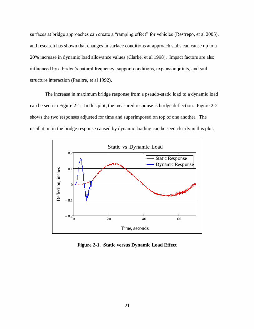
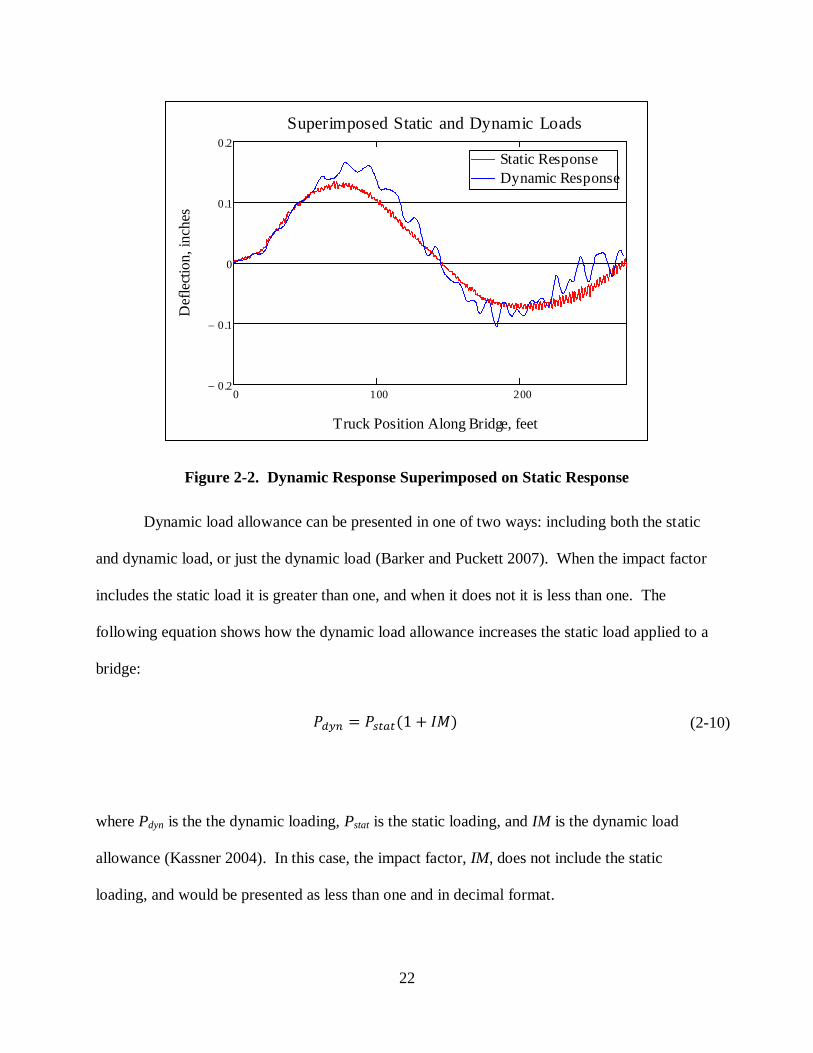
The increase in maximum bridge response from a pseudo-static load to a dynamic load

can be seen in Figure 2-1. In this plot, the measured response is bridge deflection. Figure 2-2

shows the two responses adjusted for time and superimposed on top of one another. The

oscillation in the bridge response caused by dynamic loading can be seen clearly in this plot.

Figure 2-1. Static versus Dynamic Load Effect

0 20 40 600.2

0.1

0

0.1

0.2

Static Response

Dynamic Response

Static vs Dynamic Load

Time, seconds

Def

lect

ion, in

ches

22

Figure 2-2. Dynamic Response Superimposed on Static Response

Dynamic load allowance can be presented in one of two ways: including both the static

and dynamic load, or just the dynamic load (Barker and Puckett 2007). When the impact factor

includes the static load it is greater than one, and when it does not it is less than one. The

following equation shows how the dynamic load allowance increases the static load applied to a

bridge:

(2-10)

where Pdyn is the the dynamic loading, Pstat is the static loading, and IM is the dynamic load

allowance (Kassner 2004). In this case, the impact factor, IM, does not include the static

loading, and would be presented as less than one and in decimal format.

0 100 2000.2

0.1

0

0.1

0.2

Static Response

Dynamic Response

Superimposed Static and Dynamic Loads

Truck Position Along Bridge, feet

Def

lect

ion, in

ches

23

2.3.1 AASHTO Dynamic Load Allowance

The AASHTO LRFD Bridge Design Specification does not attempt to model all aspects

that affect dynamic load allowance, nor does it present empirical formulas based on bridge

geometry and design. Instead, it gives standard values used to increase static loads. Table 2-2

presents values from AASHTO Specification Table 3.6.2.1-1 for dynamic load allowance:

Table 2-2. AASHTO Dynamic Load Allowance (AASHTO 2004)

Component IM (%)

Deck joints- all limit states 75

All other components

Fatigue and fracture limit states 15

All other limit states 33

Steel girders, which are the focus of this discussion, are categorized under all other

components, all other limit states. This represents an increase of 33% above the static loading,

which would be presented either as IM = 1.33 or IM = 0.33, depending on the chosen convention.

2.3.2 Experimental Calculation of Dynamic Load Allowance

To obtain impact factors from live load test data, it is necessary to load the bridge both

statically and dynamically in the same travel path. It is commonly accepted that data recorded

during quasi-static, or creep, tests can be used as the static response when calculating dynamic

load allowance (Potisuk and Higgins 2007). Dynamic response is measured when the loading

vehicle passes at highway speeds of at least an order of magnitude larger than the quasi-static

speed, and the maximum value for a specific girder is used. Once these maximum static and

dynamic response values are recorded the dynamic load allowance is calculated using one of the

following equations:

24

(2-11)

which includes the static response, and where IM is the impact factor, Ddyn is the measured

dynamic response, and Dstat is the measured static response, or (Barker and Puckett 2007):

(2-12)

which does not include the static response, where the variables are the same as defined above

(Neely, et al 2004). Researchers have shown that either strain or deflection values can be used as

the measured response when calculating dynamic load allowance (Kassner 2004).

2.4 Bearing Rotation Behavior

Behavior of a beam is greatly influenced by the support, or boundary, conditions imposed

on it. This is evidenced by the extremely different behavior occurring among the three

commonly used theoretical boundary conditions of fixed, pinned, and roller. To know how a

bridge will perform, it is important to understand the support conditions imposed on a bridge by

its bearings. Bridge bearings need to be able to transfer reactions between the superstructure and

substructure, meeting design requirements for forces, displacements, and rotations (Huth and

Khbeis 2007). However, the theoretical conditions used in analysis and design do not exist in

real life, and all types of bridge bearings perform somewhere in between the theoretical behavior

of pure fixity and frictionless pin or roller.

25

Restrained bearing behavior has been shown to influence global bridge behavior

(Stallings and Yoo 1993; Badwan and Liang 2007), and changing bearing conditions due to

corrosion can be misinterpreted as a change in other bridge stiffness related parameters.

Unfortunately, bearing behavior is difficult to directly monitor on a constructed bridge. Some

researchers have used strain gages on girders near bearings to capture restraint moments induced

by ill-performing bridge bearings (Barker, et al 1999). As previously mentioned, other

researchers have placed multiple inclinometers on elastomeric bearings to observe their

performance under temperature induced loads.

Tests involving bearing behavior are much more easily conducted in a controlled

laboratory setting. Research has been performed on many new bridge bearings including

elastomeric, pot, spherical, and disk bearings. These tests were conducted with an applied

constant compressive load, and rotations were induced cyclically to study their performance over

multiple tests (Roeder, et al 1995). Other researchers have removed bearings from bridges after

many years in use to test their rotational resistance and restoring moment behavior in a

laboratory setting (Huth and Khbeis 2007).

2.5 Composite Action

Composite action occurs where there exists a shear connection between a bridge girder

and deck (Barker and Puckett 2007). Instead of acting as two separate entities, the shear

connection enables the girder and deck to carry load together, increasing the stiffness of the

section. Because this behavior depends on a connection between steel shear studs and the

concrete deck, deterioration may cause a decrease in the amount of composite action present in

the bridge section.

26

The amount of composite action occurring between bridge girders and deck can be

determined by examining the location of the composite section’s neutral axis. Using a transform

section analysis, it is possible to theoretically determine the location of the neutral axis for a fully

composite section, representing 100% composite action. The location of the neutral axis of the

bridge girder alone represents zero composite action. Researchers have tested the amount of

composite action occurring in bridges by comparing theoretical neutral axis locations with those

calculated from data collected during load testing (Stiller, et al 2006).

Many live load tests have used numerous strain gages or transducers along the depth of a

bridge girder to determine where the composite section’s strain profile switches from

compression to tension, which is the location of the neutral axis. However, assuming a linear

strain profile, which is a safe assumption as long as applied stresses are below the material’s

yield point, means that only two strain transducers are necessary to accurately capture this

behavior. Multiple tests have successfully determined neutral axis location of steel girder

bridges with only two strain transducers (Park, et al 2005).

2.6 Literature Review Summary

The main purpose of this literature review was to review the current state of practice for

live load testing of bridges. This included discussions on bridge characterization, testing

procedures such as load application and data collection, and the analysis of results, including

load distribution factors and dynamic load allowance. Also included in these discussions were

examples of studies looking at details of specific bridge components, such as bridge bearing

performance and neutral axis locations of composite sections. When applicable for comparison

with live load test results, design provisions have also been presented in this literature review.

27

Chapter 3: Experimental Procedure

Live load testing of the Virginia Pilot Bridge was performed over a period of three days

in October of 2009. The first day of testing, October 20, involved the instrumentation and

testing of the North Span of the bridge. Instrumentation was repositioned to the South Span on

October 21, while other researchers were conducting dynamic testing on the bridge. The South

Span of the bridge was tested on the final day, October 22, and all instrumentation was then

removed.

3.1 Desired Data

Bridge behavior can be characterized by several different stiffness related performance

parameters. When determining the live-load testing plan, it was necessary to know the

parameters needed to characterize the performance of the bridge. Researchers compiled a list of

desired parameters, and determined the data needed to obtain that information. The basic

performance parameters include girder and deck service strains, girder deflections, wheel load

distributions, dynamic load allowance, bearing rotational behavior, expansion joint behavior, and

percent of composite action occurring between the bridge deck and girders. Also necessary for

comparison purposes with future testing is temperature records on the bridge.

3.2 Bridge Instrumentation

Starting with the desired data, instrumentation was chosen and positioned on the bridge to

capture the specified behavior during testing. Instruments available for use during testing

28

included strain transducers, deflectometers, inclinometers and tilt-meters, linear variable

differential transformers (LVDTs), thermocouples, and hand-held thermometers.

3.2.1 Strain Transducers

Strains were recorded during live-load testing through the use of eighteen strain

transducers manufactured by Bridge Diagnostics Incorporated (BDI), seen in Figure 3-1.

Figure 3-1. BDI Strain Transducers

These instruments are composed of a full wheatstone bridge with four active foil strain

gages. Because the circuit is completed within the transducer, long cable lengths do not

influence the signal, which is extremely important on the long spans of the Virginia Pilot Bridge.

These transducers are calibrated by the manufacturer, and are accurate to two per cent of the

value being measured.

Transducers can be attached to both steel and concrete through the use of a two-part

epoxy, in this case Loctite glue and accelerator seen in Figure 3-2. Small metal tabs with

threaded rods are attached to the bridge surface, and the transducers are held in place with nuts.

29

Light surface preparation is performed on the bridge using a sanding pad on an electric grinder to

remove paint, rust, and other debris from the surface. Loctite 410 glue is applied to both the

surface and the tabs of the transducer, and then Loctite 7452 accelerator is sprayed on both

surfaces. Once the tabs are placed on the surface, only a few seconds are needed for proper

bonding to take place.

Figure 3-2. Loctite Two-Part Epoxy

Strain transducers were located on the bottom flanges of girders to record the maximum

possible strain. Some girders were instrumented with multiple transducers throughout their

height, allowing researchers to plot strain distributions and determine the neutral axis of the

girders. Initial testing plans called for strain gages on the bottom and top flanges, as well as the

bottom of the deck, as seen in Figure 3-3.

30

Figure 3-3. North Span Strain Transducer Arrangement

Transducers were attached to the bottom center of the bottom flange, and the bottom of

the top flange, centered on the exposed half of the flange, which is 3 13/16 in. from the web. To

place transducers on the bottom of the concrete deck it was necessary to move them away from

the girder. This was done in order to avoid the concrete haunch located between the top flange

and the deck. Transducers placed on the deck were located one inch to the side of the haunch.

After testing on the North Span was completed, it was determined that the strain transducers on

the deck would serve their purpose better on the girder webs, as illustrated in Figure 3-4. For

testing on the South Span, transducers initially planned to be placed on the deck were attached to

the web of the girders, 12 in. above the bottom flange, while instruments on the flanges were left

in the same locations.

3"

3"

1"

0"

StrainTransducers

Varies

Typical3 13/16"

31

Figure 3-4. South Span Strain Transducer Arrangement

Due to the layout of bearings, bearing stiffeners, and cross bracing, bottom flange strain

transducers at the bridge’s center support could not be attached as they were in other locations on

the bridge. The pin bearing at the center support made it impossible to locate the transducers on

the underside of the flange. On the upper side of the bottom flange, bearing stiffeners and cross

bracing connections did not allow placement at the exact center of the bridge. For this reason,

strain transducers at the center support were offset from the center of the bridge by 4 in., towards

the North Span, as seen in Figure 3-5. To line up all instrumentation at the center support, all

strain transducers were offset to match the bottom flange arrangement.

0"

StrainTransducers

12"

3 13/16"

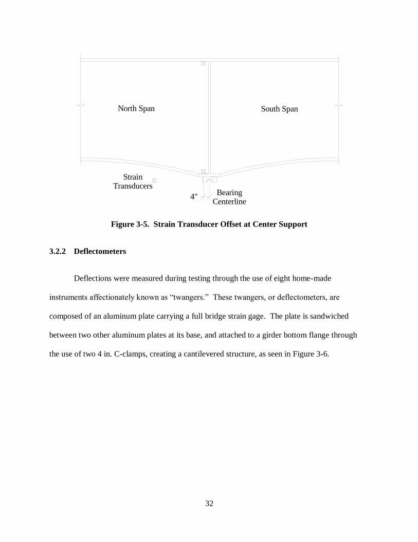
32

Figure 3-5. Strain Transducer Offset at Center Support

3.2.2 Deflectometers

Deflections were measured during testing through the use of eight home-made

instruments affectionately known as “twangers.” These twangers, or deflectometers, are

composed of an aluminum plate carrying a full bridge strain gage. The plate is sandwiched

between two other aluminum plates at its base, and attached to a girder bottom flange through

the use of two 4 in. C-clamps, creating a cantilevered structure, as seen in Figure 3-6.

StrainTransducers

BearingCenterline

4"

North Span South Span

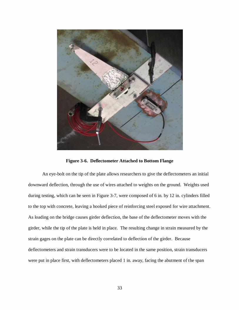
33

Figure 3-6. Deflectometer Attached to Bottom Flange

An eye-bolt on the tip of the plate allows researchers to give the deflectometers an initial

downward deflection, through the use of wires attached to weights on the ground. Weights used

during testing, which can be seen in Figure 3-7, were composed of 6 in. by 12 in. cylinders filled

to the top with concrete, leaving a hooked piece of reinforcing steel exposed for wire attachment.

As loading on the bridge causes girder deflection, the base of the deflectometer moves with the

girder, while the tip of the plate is held in place. The resulting change in strain measured by the

strain gages on the plate can be directly correlated to deflection of the girder. Because

deflectometers and strain transducers were to be located in the same position, strain transducers

were put in place first, with deflectometers placed 1 in. away, facing the abutment of the span

34

being tested. Deflectometers were calibrated in the laboratory prior to field testing, and were

shown to be accurate to the nearest 0.001 in.

Figure 3-7. Deflectometer Weight

3.2.3 Inclinometers and Tiltmeters

Bearing rotations were measured using two different types of instruments. A Rieker

SBS1U Servo inclinometer, shown in Figure 3-8, was used at the bridge’s abutment ends, while

Applied Geomechanics tiltmeters, shown in Figure 3-9, were used at the center support.

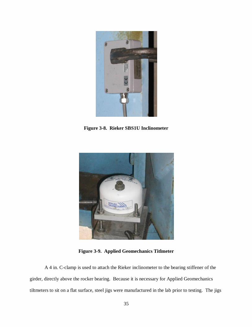
35

Figure 3-8. Rieker SBS1U Inclinometer

Figure 3-9. Applied Geomechanics Titlmeter

A 4 in. C-clamp is used to attach the Rieker inclinometer to the bearing stiffener of the

girder, directly above the rocker bearing. Because it is necessary for Applied Geomechanics

tiltmeters to sit on a flat surface, steel jigs were manufactured in the lab prior to testing. The jigs

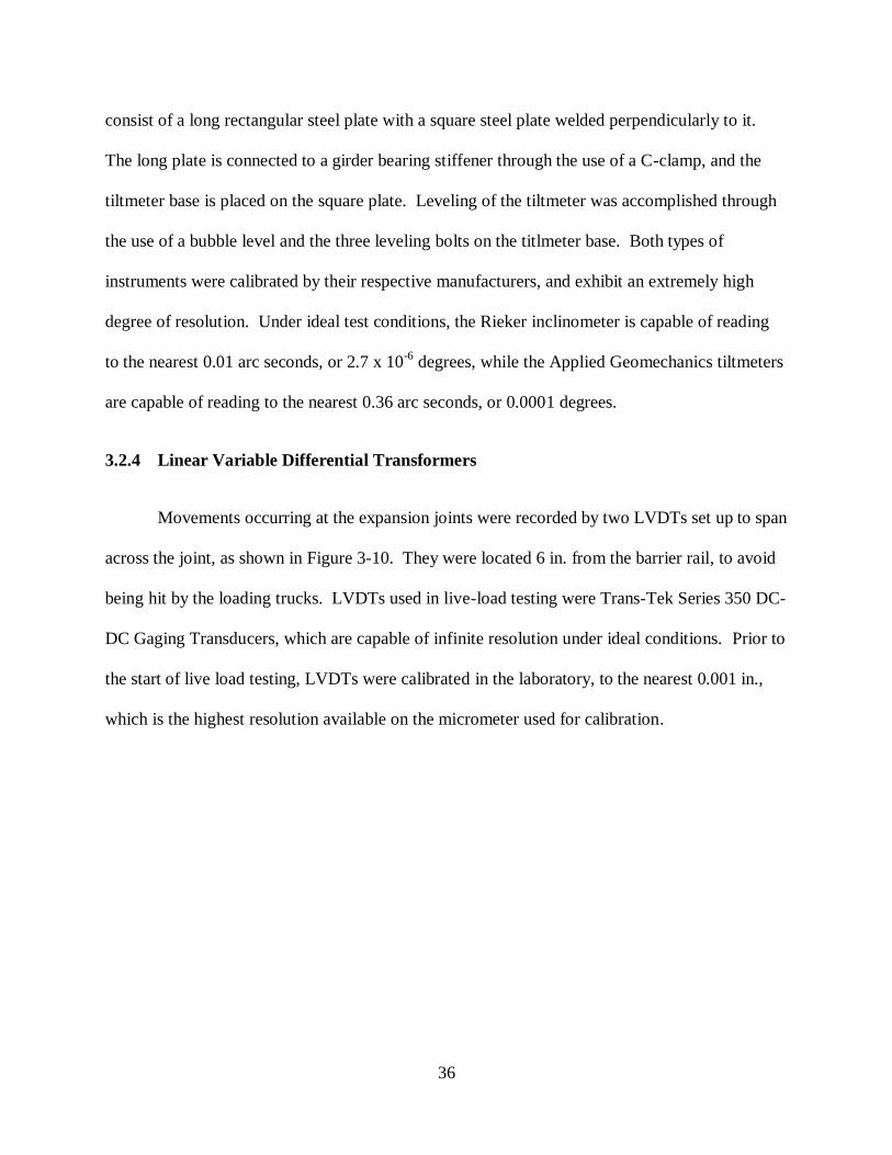
36

consist of a long rectangular steel plate with a square steel plate welded perpendicularly to it.

The long plate is connected to a girder bearing stiffener through the use of a C-clamp, and the

tiltmeter base is placed on the square plate. Leveling of the tiltmeter was accomplished through

the use of a bubble level and the three leveling bolts on the titlmeter base. Both types of

instruments were calibrated by their respective manufacturers, and exhibit an extremely high

degree of resolution. Under ideal test conditions, the Rieker inclinometer is capable of reading

to the nearest 0.01 arc seconds, or 2.7 x 10-6

degrees, while the Applied Geomechanics tiltmeters

are capable of reading to the nearest 0.36 arc seconds, or 0.0001 degrees.

3.2.4 Linear Variable Differential Transformers

Movements occurring at the expansion joints were recorded by two LVDTs set up to span

across the joint, as shown in Figure 3-10. They were located 6 in. from the barrier rail, to avoid

being hit by the loading trucks. LVDTs used in live-load testing were Trans-Tek Series 350 DC-

DC Gaging Transducers, which are capable of infinite resolution under ideal conditions. Prior to

the start of live load testing, LVDTs were calibrated in the laboratory, to the nearest 0.001 in.,

which is the highest resolution available on the micrometer used for calibration.

37

Figure 3-10. LVDT Positioning at Expansion Joint

LVDTs were held in place through the use of nuts and washers through a hole in a cold-

formed steel angle. This angle held the LVDTs at a height of 1.5 in. above the concrete deck, as

seen in Figure 3-11. Contact with the plunger of the LVDT was made across the joint with

another cold-formed steel angle. Both angles were attached to the deck with two-part epoxy, and

held in place with a weighted object until the epoxy set.

38

Figure 3-11. LVDT Angle Dimensions

3.2.5 Thermocouples and Thermometers

Temperature measurements were made on the superstructure through the use of Type-T

thermocouples located on the bottom flanges of girders number one and three. Type-T

thermocouples have a listed limit of error of 1 degree Fahrenheit, which is the maximum non-

linearity that will be experienced. This arrangement recorded temperatures of an exterior and an

interior girder. On the deck, temperature measurements were made using an Omega handheld

thermometer, which is accurate to 2 per cent of the value being read.

3.2.6 Truck Locating Marker

Truck positioning along the length of the bridge was recorded in the data through the use

of a marker device. The marker used during testing was a modified crack gage, attached to a

very long lead wire. The crack gage is composed of an omega shaped piece of thin metal with a

foil strain gage fixed to it, as seen in Figure 3-12. The marker was squeezed as the front tires of

the truck reached predetermined points along the length of the bridge, keeping track of the

loading location.

.125"

3.5"

2.5"

1.5"

Ø .563"

2"

9/16"

1/8"

2" Varies 3.5" Varies

39

Figure 3-12. Location Marker Tool

3.2.7 Instrumentation Layout

The location of instruments along the length of the bridge was chosen to maximize the

magnitude of the data values being recorded. From initial finite element models, it was

determined that strain transducers and deflectometers should be located at four tenths of a single

span length, or 54 ft-10 in. from the abutment. Other instrumentation was placed either at the

abutment or center support, as needed. Two deflectometers were also placed at two tenths of the

span length, or 27 ft-5 in. from the abutment, to help in the process of refining finite element

models. Due to limitations imposed by the number of channels on the data acquisition system,

the number of instruments available, and restrictions to access due to lane closures, it was

determined that each span would be tested independently. A total of 18 strain transducers, eight

deflectometers, two LVDTs, two tiltmeters, one inclinometer, and two thermocouples were

arranged as seen in Figure 3-13 and Figure 3-14. The inclinometer located at the abutment,

40

shown in the figures on girder three, was moved between girders one, two and three during the

testing process.

Figure 3-13. North Span Instrumentation Layout

Figure 3-14. South Span Instrumentation Layout

3.3 Data Acquisition

Data acquisition was performed using a CR9000X Datalogger, shown in Figure 3-15,

from Campbell Scientific, Inc. The CR9000X is a multi-purpose system that is extremely

adaptable and capable of running multiple instrument types simultaneously. CR Basic Editor

and RTDAQ Software were used to program and operate the system. All instruments were

South Span North Span

1 2

43

56

I

I I

I

T T

T

324

648

Three Strain Transducers Strain Transducer Deflectometer

Thermocouple Inclinometer or Tiltmeter

0.4 L0.2 L

LVDT

1630 L

South Span North Span

1 2

43

56

I

I I

I

T T

T

Three Strain Transducers Strain Transducer Deflectometer

Thermocouple Inclinometer or Tiltmeter LVDT

1656

648

324

L

0.4 L

0.2 L

41

connected to the datalogger, and records were made at 100 Hz for all instruments other than

thermocouples, which were recorded at 1/10 Hz. The program used with the CR9000X during

live load testing can be found in Appendix A.

Figure 3-15. CR9000X Data Acquisition System

3.4 Instrument Calibration

Prior to performing field testing, calibration data for each instrument was recorded.

Some instruments, such as the inclinometers, tiltmeters, strain transducers, thermocouples, and

thermometers were calibrated by their respective manufacturers, and calibration values were

input into the CR Basic Editor code as were appropriate.

As previously mentioned, deflectometers and LVDTs were calibrated by hand before

heading into the field. Each instrument was connected to the CR9000X Datalogger with its

42

respective cable. RTDAQ’s Calibration Wizard was used for a two point calibration of each

instrument. Deflectometers were attached to a table top using C-clamps, and the wire used for

predeflection was attached to a large caliper. LVDTs were calibrated through the use of a

calibration jig and micrometer. After calibration was completed, each instrument was checked

for accuracy and Calibration History files were stored in the CR9000X.

3.5 Loading Procedure

3.5.1 Truck Description

Loading of the bridge was provided through the use of two loaded Virginia Department

of Transportation (VDOT) dump trucks. Both three-axle trucks were loaded with gravel from

the Vulcan Materials Company’s Manassas Quarry, to loads of approximately 50 kips. Before

leaving the quarry, the axles of both trucks were weighed individually to determine the load

distribution. Both vehicles distributed about 68 per cent of their load to the rear axles, and 32 per

cent to the front axles, as seen in Figure 3-16. The trucks’ axle dimensions were measured and

recorded when they arrived to the testing site. Dimensions of both trucks were identical, and the

measurements can be seen in the sketch in Figure 3-17.

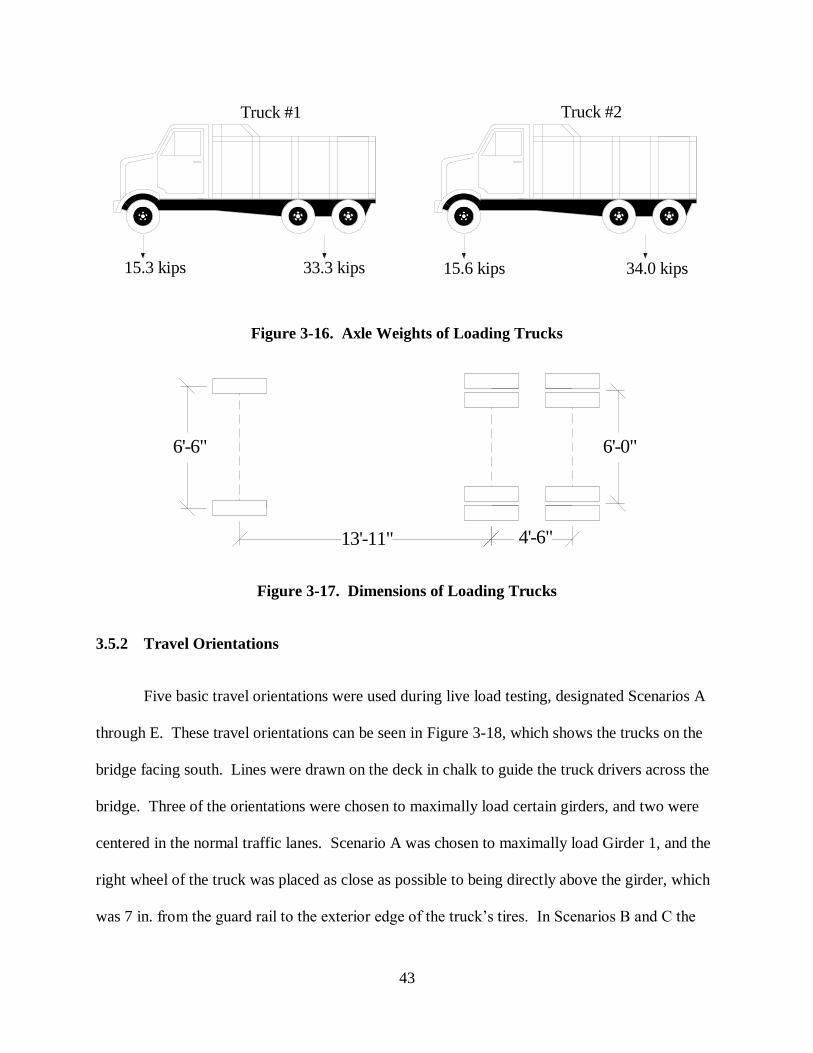
43

Figure 3-16. Axle Weights of Loading Trucks

Figure 3-17. Dimensions of Loading Trucks

3.5.2 Travel Orientations

Five basic travel orientations were used during live load testing, designated Scenarios A

through E. These travel orientations can be seen in Figure 3-18, which shows the trucks on the

bridge facing south. Lines were drawn on the deck in chalk to guide the truck drivers across the

bridge. Three of the orientations were chosen to maximally load certain girders, and two were

centered in the normal traffic lanes. Scenario A was chosen to maximally load Girder 1, and the

right wheel of the truck was placed as close as possible to being directly above the girder, which

was 7 in. from the guard rail to the exterior edge of the truck’s tires. In Scenarios B and C the

15.3 kips 33.3 kips 15.6 kips 34.0 kips

Truck #1 Truck #2

80

170 50

706'-6"

13'-11" 4'-6"

6'-0"

44

two trucks were used together, spaced 36 in. apart, center to center of their front tires, from one

another. Scenario B maximally loads Girder 2, and Scenario C was designed to load Girder 3.

In both of these scenarios, the left wheel of the right loading truck was intended to be directly

above the target girder. Unfortunately, when the lines were drawn for Scenario C, a mis-

measurement took place and the trucks were positioned 1 ft to the right of their intended

location. Scenarios D and E again use a single truck, centered in the right and left lanes,

respectively.

Figure 3-18. Travel Orientations of Loading Trucks Facing South

3.5.3 Loading Speeds

Three types of loadings were performed at different speeds during live-load testing. For

all loading scenarios trucks were driven across the bridge at 2-3 mph for quasi-static, or creep,

tests. These tests took between 55 and 70 seconds to perform. Highway tests were performed

Scenario A

Scenario B

Scenario D

Scenario E

Scenario C

6 2345 1

7"

36"

36"

12"

Clear Spacing

Center to Center

Center to Center

45

for Scenario D, where the trucks were driven as close as possible to the posted speed limit. Due

to traffic restrictions, the maximum speeds that the truck drivers could obtain was roughly 25

miles per hour, resulting in truck crossings ranging from eight to ten seconds. This is a fair

approximation of standard traffic speed on this part of Route 15 because of the layout of traffic

lights and intersections surrounding the bridge. However, the trucks driven at highway speeds

were not consistently centered in the traffic lane, making comparisons with quasi-static test data

unreliable. The third type of tests performed were static tests, where the trucks were completely

stopped on the bridge. Trucks were stopped at 0.25 and 0.65 times the span length, which is 34

ft-3 in. and 54 ft-10 in., respectively, from the abutment end of the bridge. For comparison

purposes with finite element models, the trucks were always oriented facing the center support

during static testing.

Ideally, testing of each combination of loading scenario and speed would have been

performed five times. However, time restraints due to traffic control limited the number of tests

that could be performed. Table 3-1 shows the number of tests performed for each combination

of load and speed. Note that data set 24 is missing for North Span testing. Although data was

recorded, a communication error occurred resulting in ambient traffic on the bridge. This data

set has been discarded.

46

Table 3-1. Test Log of North and South Span Live Load Testing

Data Set Number Span Truck Speed Orientation

1-3 North Creep A

4-7 North Creep B

8-11 North Creep D

12-15 North Creep E

16-19 North Creep C

20-21 North Static A

22 North Static B

23 North Static C

25-26 North Highway D

1-4 South Creep A

5-8 South Creep B

9-12 South Creep E

13-16 South Creep D

17-20 South Creep C

21-24 South Highway D

25-26 South Static A

27-28 South Static B

3.6 Data Organization

Upon completion of each live load test, all data was downloaded from the CR9000X and

stored on a personal computer in the form of a text data file. Large file sizes due to the high

sampling rate and length of tests made it difficult to process the data in Excel. For this reason,

MathCad was chosen as a data processor and plotter.

Data recorded during live load testing can include noise due to electrical interference,

both internally and externally generated. To counteract this, the CR9000X was unplugged from

the generator for each test. During this time the CR9000X ran on its internal battery, capable of

producing 14 Amp-hours of direct current. However, the data still exhibited noise, and in some

cases this noise was quite significant. A mistake in the CR Basic Program written to run the

47

CR9000X during testing created noise in all strain transducers being used. Due to this noise,

data filtering was necessary.

A routine was written in MathCad that filtered the data using a running average. A

running average is useful because the number of data points does not decrease, allowing the

relationship between data and the truck location marker to be maintained. The routine used to

filter the data, which can be seen in Appendix B, was made adjustable by varying the number of

data points to be used in an average. Data was plotted and filtered to the point where individual

points could be accurately chosen from the data set. An example of a filtered data plot, showing

multiple iterations of filtering, can be seen in Figure 3-19. For comparison purposes, these plots

have been offset from one another by 20µε. The 20 Point Average line represents the baseline,

and 20µε and 40µε have been added to the 10 Point Average line and the Raw Data line,

respectively.

Figure 3-19. Filtering Plot of Test Data

0 100 20050

0

50

100

150

Raw Data

10 Point Average

20 Point Average

Filtering Plot

Truck Position Along Bridge, feet

Str

ain, m

icro

stra

in

48

Another necessity during the analysis of live load testing data was to zero values at the

beginning of tests. Although instruments were periodically zeroed during testing, some

instruments needed adjustment throughout the day. For example, on the first day of testing a

loading truck hit an LVDT monitoring deck joint movements. This caused the damaged LVDT

to read off scale. A programming glitch in the data acquisition system does not allow zeroing of

a channel if any instrument in that channel is reading off scale. Because all LVDTs were

connected on the same channel of the CR9000X, other LVDTs could not be zeroed. For this

reason a MathCad routine, found in Appendix B, was needed to zero the data during analysis.

This routine averages the first one hundred data points, which is one second of recording time

that occurs before load was applied to the bridge. This average value is then subtracted from all

data points in the set to zero the data. An example of data zeroing can be seen in Figure 3-20.

Figure 3-20. Zeroing Plot of Test Data

Once data was properly filtered and zeroed, points could be selected from the plots for

data analysis. Values were taken either at maximum or minimum points, or at specific loading

0 100 200

0

0.01

Raw

Zeroed

Zeroing Plot

Truck Position Along Bridge, feet

Dis

pla

cem

ent, inch

es

49

locations known from truck marker data, depending on what was needed for analysis. These

selected data points were then used in the analysis process.

3.7 Data Reporting

The accuracy and resolution of each measurement has determined the level of results

presented. Tiltmeters located at the center support produced values of much higher resolution

than the worst-case scenario values given by the manufacturer. Although LVDTs were only

calibrated to 0.001 in., they possess excellent linearity and are capable of much higher resolution

with a two point calibration.

Resolution of data reported in the following chapters is as follows:

Strains reported to the tenth of a microstrain

Deflections reported to the thousandth of an inch

Rotations reported to the ten-thousandth of a degree

Joint displacements reported to the ten-thousandth of an inch

Thermocouple measurements reported to tenth of a degree Fahrenheit

Handheld thermometer measurements reported to a degree Fahrenheit

50

Chapter 4: Experimental Results

The majority of the results presented in this chapter were recorded during pseudo-static,

or creep, tests. Results of highway speed tests for strains and deflections are discussed in Section

4.5. Static testing results are presented for bearing rotations in Sections 4.7. Unless stated

otherwise, all plots depict average data from all tests of the same loading scenario. Full data

tables of experimental results can be found in Appendix C.

4.1 Service Strain and Deflection Results at Four Tenths of Span Length

4.1.1 Service Strain Results

The following tables present the peak service strain and service deflection results

recorded at four tenths of the span length on the bottom flange of each of the six girders for each

loading scenario during pseudo-static testing. Peak values are the maximum recorded values

during each individual test. These peak values were recorded when the loading trucks were

directly above instrumentation, causing tension and downward deflection, as well as when the

trucks were on the adjacent span, causing compression and uplift in the girders. Presented are

the average responses over all similar testing cases, the maximum recorded values, the standard

deviation of the data, and the number of tests conducted.

All strain values are presented in microstrain, while the units of deflection are inches.

Values are presented as positive when strain is in tension and deflection is downward, and

negative when uplift occurs and strain is in compression.

Table 4-1 shows data recorded during testing of the North and South Spans during

loading Scenario A. As expected for this load case, Girder 1 produced the largest average strain

51

on each span, both in tension and compression. Values of 84.2 με and -19.6 με were recorded on

the North Span, while values of 72.7 με and -17.1 με were measured on the South Span.

Table 4-1. Scenario A Service Strains

Span 1 2 3 4 5 6

84.2 59.7 27.8 13.3 1.0 0.0

84.4 60.2 28.6 14.2 1.9 0.0

0.2 0.8 0.9 0.8 0.9 0.0

-19.6 -14.3 -11.0 -10.1 -4.5 0.0

-19.9 -16.1 -12.1 -10.9 -5.0 0.0

0.3 1.7 1.0 1.0 0.9 0.0

72.7 61.3 29.9 15.2 3.3 0.0

74.3 61.8 30.9 16.1 4.0 0.0

1.5 0.6 0.8 0.6 0.5 0.0

-17.1 -13.8 -12.0 -10.0 -3.3 0.0

-18.6 -14.5 -12.4 -10.5 -4.0 0.0

1.4 0.9 0.3 0.5 0.5 0.0

Maximum

Standard Deviation

Number of Tests 4

South

Standard Deviation

Compression Strains (με)

Average

Maximum

Loading Scenario A

Number of Tests 3

Standard Deviation

Compression Strains (με)

Average

Average

Maximum

Standard Deviation

Girder Number

Tension Strains (με)

North

Tension Strains (με)

Average

Maximum

Table 4-2 presents service strain results for both spans under loading Scenario B. This

loading scenario was intended to place the maximum load on Girder 2, but as can be seen in the

table, on the North Span Girder 1 again produced the largest strain response, with average values

of 110 με and -30.1 με. On the South Span, Girder 2 achieved the maximum average tensile

value of 105 με. In compression the response was more evenly distributed, and Girder 1

experienced the largest strain with an average value of -25.9 με.

52

Table 4-2. Scenario B Service Strains

Span 1 2 3 4 5 6

110 105.9 84.5 46.6 22.1 11.8

112 106.7 86.1 49.0 25.8 13.5

1.3 0.7 1.4 1.7 2.7 1.3

-30.1 -23.8 -18.8 -15.5 -13.1 -9.9

-30.9 -25.4 -21.1 -15.9 -16.0 -11.6

0.8 1.2 1.5 0.5 2.4 1.4

91.4 105.3 85.0 50.1 24.1 8.8

92.8 107.2 86.4 50.5 25.6 9.0

1.8 1.8 1.3 0.5 1.3 0.5

-25.9 -21.4 -17.8 -15.6 -12.2 -9.0

-26.8 -22.3 -18.3 -16.3 -12.8 -10.0

1.0 0.9 0.8 0.8 0.5 0.8

4

South

Standard Deviation

Compression Strains (με)

Average

Average

Maximum

Standard Deviation

Number of Tests 4

Tension Strains (με)

Average

Maximum

Girder Number

Tension Strains (με)

North

Loading Scenario B

Average

Maximum

Standard Deviation

Compression Strains (με)

Maximum

Standard Deviation

Number of Tests

Service strain results for loading Scenario C are presented in Table 4-3. When the trucks

were located on the instrumented spans the greatest responses were recorded in Girder 3. The

average strain recorded was 95.3 με and 90.8 με on the North and South Spans, respectively.

However, when the loading vehicles were traveling on the adjacent span, the compression caused

in the girders was more evenly distributed and Girder 1 experienced the highest average strain in

compression, which was -24.2 με and -19.8 με for the North and South Spans, respectively.

53

Table 4-3. Scenario C Service Strains

Span 1 2 3 4 5 6

57.8 81.5 95.3 76.2 43.7 30.0

58.9 82.2 96.4 78.4 45.1 30.9

1.1 0.6 1.3 1.8 1.6 1.1

-24.2 -20.4 -18.7 -15.8 -15.0 -16.8

-24.9 -21.3 -19.1 -16.1 -15.8 -18.5

0.5 0.6 0.4 0.2 0.7 1.9

48.4 75.9 90.8 81.6 46.8 28.2

49.2 78.3 91.2 82.2 47.4 28.6

0.8 1.6 0.3 0.6 0.6 0.5

-19.8 -19.2 -17.6 -16.3 -17.0 -17.6

-20.5 -20.2 -18.6 -17.6 -17.9 -18.4

0.9 0.8 1.0 1.1 0.9 0.7

Compression Strains (με)

4

Loading Scenario C

Average

Maximum

Standard Deviation

Number of Tests

Standard Deviation

Number of Tests

Average

Maximum

Maximum

Standard Deviation

Girder Number

Tension Strains (με)

North

4

South

Tension Strains (με)

Maximum

Standard Deviation

Compression Strains (με)

Average

Average

Loading Scenarios D and E represent vehicles traveling in the right and left travel lanes,

respectively. Table 4-4 presents the strain data recorded during load Scenario D. For this load

case, Girder 3 experienced the maximum recorded tension strains, with average values of 56.1 με

on the North Span and 54.9 με on the South Span. Once again, compression strains were more

evenly distributed, and Girder 1 experienced the largest responses at -14.3 με and -12.8 με for the

North and South Spans, respectively. Data recorded during loading Scenario E is presented in

Table 4-5. For this case, Girder 5 recorded the largest tension strains, with average values of

55.3 με and 56.0 με, while Girder 6 produced the largest compression strains, reaching values of

-16.5 με and -16.3 με for the North and South Spans, respectively.

54

Table 4-4. Scenario D Service Strains

Span 1 2 3 4 5 6

29.1 41.8 56.1 38.9 20.9 13.0

30.0 42.9 57.4 39.6 21.2 13.9

0.6 0.9 1.2 0.6 0.2 0.8

-14.3 -12.4 -11.1 -9.7 -9.5 -9.8

-15.6 -14.0 -11.5 -11.7 -11.2 -11.2

1.2 1.6 0.6 1.6 1.2 1.3

25.2 38.8 54.9 40.2 21.8 14.6

25.9 39.3 55.5 41.0 22.5 15.1

0.7 0.5 0.6 0.9 1.1 0.7

-12.8 -11.6 -9.7 -9.7 -10.3 -10.2

-13.1 -12.8 -10.8 -9.8 -10.8 -11.3

0.3 0.8 0.9 0.1 0.7 0.8

Girder Number

North

Maximum

Maximum

Standard Deviation

Average

Loading Scenario D

Compression Strains (με)

4

Tension Strains (με)

South

Tension Strains (με)

Maximum

Standard Deviation

Compression Strains (με)

Average

Maximum

Standard Deviation

Number of Tests

Average

4

Standard Deviation

Number of Tests

Average

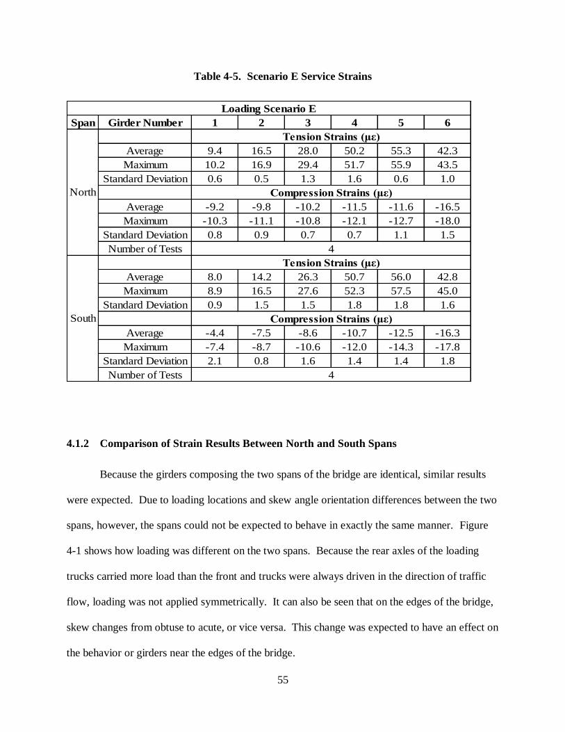
55

Table 4-5. Scenario E Service Strains

Span 1 2 3 4 5 6

9.4 16.5 28.0 50.2 55.3 42.3

10.2 16.9 29.4 51.7 55.9 43.5

0.6 0.5 1.3 1.6 0.6 1.0

-9.2 -9.8 -10.2 -11.5 -11.6 -16.5

-10.3 -11.1 -10.8 -12.1 -12.7 -18.0

0.8 0.9 0.7 0.7 1.1 1.5

8.0 14.2 26.3 50.7 56.0 42.8

8.9 16.5 27.6 52.3 57.5 45.0

0.9 1.5 1.5 1.8 1.8 1.6

-4.4 -7.5 -8.6 -10.7 -12.5 -16.3

-7.4 -8.7 -10.6 -12.0 -14.3 -17.8

2.1 0.8 1.6 1.4 1.4 1.8

South

Tension Strains (με)

Maximum

Standard Deviation

Compression Strains (με)

Average

Maximum

Standard Deviation

Number of Tests

North

Tension Strains (με)

Compression Strains (με)

4

Loading Scenario E

Girder Number

Average

Average

4

Standard Deviation

Number of Tests

Average

Maximum

Maximum

Standard Deviation

4.1.2 Comparison of Strain Results Between North and South Spans

Because the girders composing the two spans of the bridge are identical, similar results

were expected. Due to loading locations and skew angle orientation differences between the two

spans, however, the spans could not be expected to behave in exactly the same manner. Figure

4-1 shows how loading was different on the two spans. Because the rear axles of the loading

trucks carried more load than the front and trucks were always driven in the direction of traffic

flow, loading was not applied symmetrically. It can also be seen that on the edges of the bridge,

skew changes from obtuse to acute, or vice versa. This change was expected to have an effect on

the behavior or girders near the edges of the bridge.

56

Figure 4-1. Loading and Bridge Geometry Differences

Plots in Figure 4-2 through Figure 4-6 compare data recorded on the North Span versus

that recorded on the South Span. Comparisons are made with tension data only. Distribution of

load was influenced by both spans when the loading truck was located on the span adjacent to

the instrumented span. For this reason compression data is neglected in these comparisons.

Tension strain values are more direct indicators of the performance of the individual span due to

the load being present directly above instrumentation.

As expected, it seems that the behavior of the North and South Spans are very similar.

The only major discrepancies can be seen in Figure 4-2 and Figure 4-3, where the recorded

strains for Girder 1 are not similar. For loading Scenario B, this difference is significant enough

to cause the maximally loaded girder to differ between the two spans. One possible explanation

for this difference in behavior is the previously mentioned change in angle of skew. On the

North Span, Girders 1 and 2 are in an obtuse angle of skew, while on the South Span the angle is

acute. This causes a change in relative stiffness between the two girders, and could possibly

cause this change in behavior.

South Span North Span

Direction of Traffic

0.4 L 0.4 L Center Support

Acute Angle Obtuse Angle

57

Figure 4-2. Scenario A, Span Comparison of Strain at Four Tenths of Span

Figure 4-3. Scenario B, Span Comparison of Strain at Four Tenths of Span

0.0

10.0

20.0

30.0

40.0

50.0

60.0

70.0

80.0

90.0

123456

Str

ain

, m

icro

stra

in

Girder Number

Scenario A Strain Comparison

North Span

South Span

0.0

20.0

40.0

60.0

80.0

100.0

120.0

123456

Str

ain

, m

icro

stra

in

Girder Number

Scenario B Strain Comparison

North Span

South Span

58

Figure 4-4. Scenario C, Span Comparison of Strain at Four Tenths of Span

Figure 4-5. Scenario D, Span Comparison of Strain at Four Tenths of Span

0.0

20.0

40.0

60.0

80.0

100.0

120.0

123456

Str

ain

, m

icro

stra

in

Girder Number

Scenario C Strain Comparison

North Span

South Span

0.0

10.0

20.0

30.0

40.0

50.0

60.0

123456

Str

ain

, m

icro

stra

in

Girder Number

Scenario D Strain Comparison

North Span

South Span

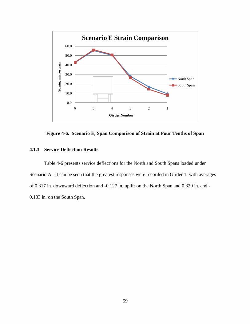
59

Figure 4-6. Scenario E, Span Comparison of Strain at Four Tenths of Span

4.1.3 Service Deflection Results

Table 4-6 presents service deflections for the North and South Spans loaded under

Scenario A. It can be seen that the greatest responses were recorded in Girder 1, with averages

of 0.317 in. downward deflection and -0.127 in. uplift on the North Span and 0.320 in. and -

0.133 in. on the South Span.

0.0

10.0

20.0

30.0

40.0

50.0

60.0

123456

Str

ain

, m

icro

stra

in

Girder Number

Scenario E Strain Comparison

North Span

South Span

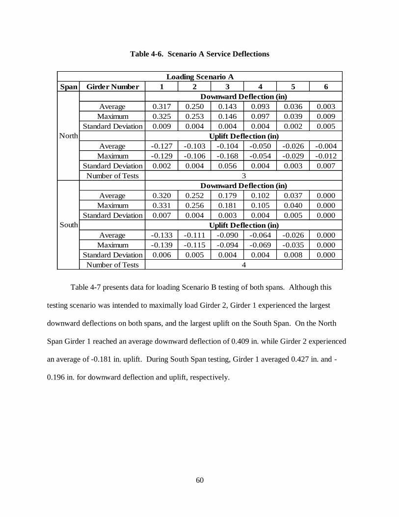
60

Table 4-6. Scenario A Service Deflections

Span 1 2 3 4 5 6

0.317 0.250 0.143 0.093 0.036 0.003

0.325 0.253 0.146 0.097 0.039 0.009

0.009 0.004 0.004 0.004 0.002 0.005

-0.127 -0.103 -0.104 -0.050 -0.026 -0.004

-0.129 -0.106 -0.168 -0.054 -0.029 -0.012

0.002 0.004 0.056 0.004 0.003 0.007

0.320 0.252 0.179 0.102 0.037 0.000

0.331 0.256 0.181 0.105 0.040 0.000

0.007 0.004 0.003 0.004 0.005 0.000

-0.133 -0.111 -0.090 -0.064 -0.026 0.000

-0.139 -0.115 -0.094 -0.069 -0.035 0.000

0.006 0.005 0.004 0.004 0.008 0.000

4

Standard Deviation

Number of Tests 3

Loading Scenario A

Girder Number

North

Downward Deflection (in)

Average

South

Downward Deflection (in)

Average

Maximum

Standard Deviation

Maximum

Standard Deviation

Uplift Deflection (in)

Average

Maximum

Uplift Deflection (in)

Average

Maximum

Standard Deviation

Number of Tests

Table 4-7 presents data for loading Scenario B testing of both spans. Although this

testing scenario was intended to maximally load Girder 2, Girder 1 experienced the largest

downward deflections on both spans, and the largest uplift on the South Span. On the North

Span Girder 1 reached an average downward deflection of 0.409 in. while Girder 2 experienced

an average of -0.181 in. uplift. During South Span testing, Girder 1 averaged 0.427 in. and -

0.196 in. for downward deflection and uplift, respectively.

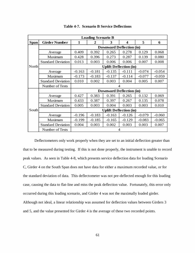
61

Table 4-7. Scenario B Service Deflections

Span 1 2 3 4 5 6

0.409 0.392 0.265 0.278 0.129 0.068

0.428 0.396 0.273 0.287 0.139 0.080

0.013 0.003 0.006 0.006 0.007 0.008

-0.163 -0.181 -0.135 -0.111 -0.074 -0.054

-0.173 -0.183 -0.137 -0.114 -0.077 -0.059

0.010 0.002 0.003 0.004 0.005 0.007

0.427 0.383 0.391 0.265 0.132 0.069

0.433 0.387 0.397 0.267 0.135 0.078

0.005 0.003 0.004 0.003 0.003 0.010

-0.196 -0.183 -0.163 -0.126 -0.079 -0.060

-0.199 -0.185 -0.165 -0.129 -0.083 -0.065

0.004 0.003 0.002 0.003 0.003 0.007

Number of Tests 4

South

Standard Deviation

Uplift Deflection (in)

Average

Maximum

Standard Deviation

Average

Maximum

Standard Deviation

Number of Tests 4

Downward Deflection (in)

Average

Maximum

Loading Scenario B

Girder Number

North

Downward Deflection (in)

Average

Maximum

Standard Deviation

Uplift Deflection (in)

Deflectometers only work properly when they are set to an initial deflection greater than

that to be measured during testing. If this is not done properly, the instrument is unable to record

peak values. As seen in Table 4-8, which presents service deflection data for loading Scenario

C, Girder 4 on the South Span does not have data for either a maximum recorded value, or for

the standard deviation of data. This deflectometer was not pre-deflected enough for this loading

case, causing the data to flat-line and miss the peak deflection value. Fortunately, this error only

occurred during this loading scenario, and Girder 4 was not the maximally loaded girder.

Although not ideal, a linear relationship was assumed for deflection values between Girders 3

and 5, and the value presented for Girder 4 is the average of these two recorded points.

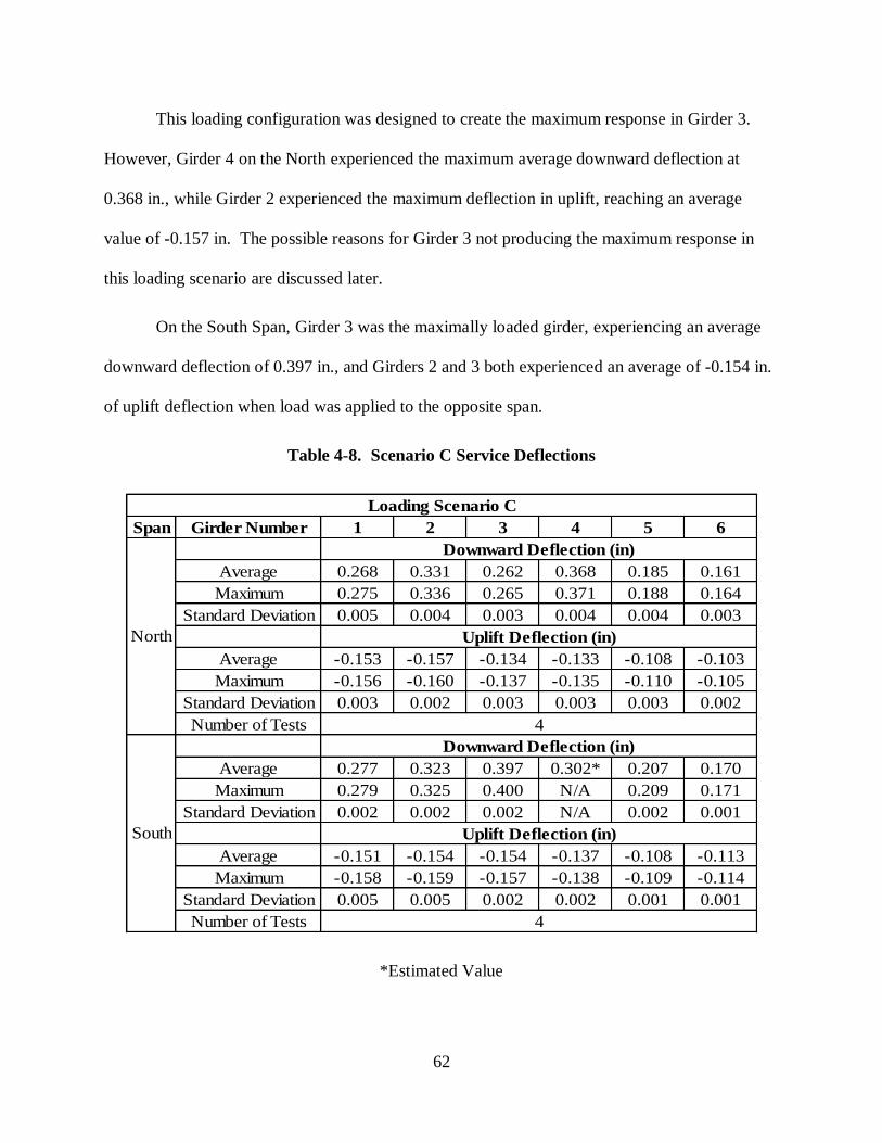
62

This loading configuration was designed to create the maximum response in Girder 3.

However, Girder 4 on the North experienced the maximum average downward deflection at

0.368 in., while Girder 2 experienced the maximum deflection in uplift, reaching an average

value of -0.157 in. The possible reasons for Girder 3 not producing the maximum response in

this loading scenario are discussed later.

On the South Span, Girder 3 was the maximally loaded girder, experiencing an average

downward deflection of 0.397 in., and Girders 2 and 3 both experienced an average of -0.154 in.

of uplift deflection when load was applied to the opposite span.

Table 4-8. Scenario C Service Deflections

Span 1 2 3 4 5 6

0.268 0.331 0.262 0.368 0.185 0.161

0.275 0.336 0.265 0.371 0.188 0.164

0.005 0.004 0.003 0.004 0.004 0.003

-0.153 -0.157 -0.134 -0.133 -0.108 -0.103

-0.156 -0.160 -0.137 -0.135 -0.110 -0.105

0.003 0.002 0.003 0.003 0.003 0.002

0.277 0.323 0.397 0.302* 0.207 0.170

0.279 0.325 0.400 N/A 0.209 0.171

0.002 0.002 0.002 N/A 0.002 0.001

-0.151 -0.154 -0.154 -0.137 -0.108 -0.113

-0.158 -0.159 -0.157 -0.138 -0.109 -0.114

0.005 0.005 0.002 0.002 0.001 0.001Standard Deviation

Number of Tests 4

South

Downward Deflection (in)

Average

Maximum

Standard Deviation

Uplift Deflection (in)

Average

Maximum

Uplift Deflection (in)

Average

Maximum

Standard Deviation

Number of Tests 4

Loading Scenario C

Girder Number

North

Downward Deflection (in)

Average

Maximum

Standard Deviation

*Estimated Value

63

Table 4-9 and Table 4-10 present service deflection data from both spans with loading

centered in the right and left traffic lanes, respectively. When the load truck traveled in the right

traffic lane, which is Scenario D, Girders 2 and 4 of the North Span experienced the maximum

average downward deflection, with a value of 0.186 in. On the South Span, however, Girder 3

was maximally loaded, reaching an average downward deflection of 0.228 in. In uplift on the

North Span, Girder 2 recorded the largest response with an average of -.081 in., while Girder 1

of the South Span experienced the most uplift, reaching an average value of -0.086 in. Under

loading Scenario E, Girder 4 experienced the maximum average downward deflection on the

North Span, reaching a value of 0.227 in. On the South Span, Girder 6 produced the maximum

response, reaching an average downward deflection of 0.222 in. On both spans Girder 6

produced the largest uplift, reaching -0.105 in. and -0.111 in. for the North and South Spans,

respectively.

64

Table 4-9. Scenario D Service Deflections

Span 1 2 3 4 5 6

0.137 0.186 0.178 0.186 0.103 0.073

0.139 0.186 0.180 0.189 0.105 0.075

0.002 0.000 0.002 0.002 0.003 0.003

-0.080 -0.081 -0.068 -0.066 -0.053 -0.050

-0.081 -0.083 -0.070 -0.068 -0.055 -0.053

0.002 0.003 0.002 0.002 0.002 0.003

0.149 0.189 0.228 0.192 0.107 0.081

0.152 0.192 0.233 0.199 0.111 0.084

0.002 0.002 0.004 0.005 0.003 0.003

-0.086 -0.084 -0.083 -0.075 -0.055 -0.057

-0.090 -0.088 -0.087 -0.077 -0.056 -0.058

0.003 0.003 0.003 0.002 0.001 0.001

Standard Deviation

Uplift Deflection (in)

Average

Maximum

Standard Deviation

Loading Scenario D

Girder Number

North

Downward Deflection (in)

Average

Maximum

Average

Maximum

Standard Deviation

Number of Tests 4

Number of Tests 4

South

Downward Deflection (in)

Average

Maximum

Standard Deviation

Uplift Deflection (in)

65

Table 4-10. Scenario E Service Deflections

Span 1 2 3 4 5 6

0.044 0.089 0.127 0.227 0.174 0.208

0.046 0.093 0.131 0.234 0.175 0.217

0.002 0.004 0.004 0.006 0.002 0.007

-0.045 -0.055 -0.065 -0.085 -0.088 -0.105

-0.066 -0.057 -0.066 -0.086 -0.090 -0.108

0.014 0.002 0.001 0.001 0.003 0.003

0.044 0.087 0.149 0.216 0.193 0.222

0.048 0.092 0.156 0.227 0.206 0.238

0.004 0.004 0.005 0.007 0.009 0.011

-0.045 -0.054 -0.068 -0.082 -0.084 -0.111

-0.059 -0.066 -0.077 -0.090 -0.091 -0.119

0.009 0.009 0.008 0.010 0.011 0.012

Loading Scenario E

Girder Number

North

Downward Deflection (in)

Average

Maximum

Standard Deviation

Uplift Deflection (in)

Average

Maximum

Standard Deviation

Number of Tests 4

South

Downward Deflection (in)

Average

Maximum

Standard Deviation

Uplift Deflection (in)

Average

Maximum

Standard Deviation

Number of Tests 4

4.1.4 Comparison of Deflection Results Between North and South Spans

Girder 3 on the North Span exhibited unexpected deflection behavior. It was expected

that recorded deflection values would, like strain values, be similar for each span. However,

values recorded on Girder 3 of the North Span are consistently lower than those from the South

Span, and differ significantly from strain data as well. This unexpected difference can be seen in

Figure 4-7, which presents the average service deflection results under loading Scenario A for

each span. In this plot, all other girders experience very similar deflections.

66

Figure 4-7. Scenario A, Span Comparison of Deflection at Four Tenths of Span

The most common error when installing deflectometers is too little initial deflection,

making the instrument unable to record peak values, as was discussed in the presentation of

South Span deflection data. By looking at the original data plots of Girder 3 deflection however,

this can be ruled out. Too little initial deflection is indicated by a flat area in the data, and the

deflection plots for Girder 3 show smooth curves. The calibrations of all deflectometers were

verified in the lab upon completion of testing. This ruled out the possibility of a damaged

instrument influencing results. Another possibility is that the deflectometer was initially given

too much deflection. This could possibly force the strain gage located on the deflectometer plate

out of its linear range, creating an error in the deflection data.

Unfortunately, Girder 3 was intended to be the maximally loaded girder for both loading

Scenarios C and D. If this were not the case, the recorded deflection values could be thrown out,

and new deflections could be estimated from values of adjacent girders. Because Girder 3 is

0.000

0.050

0.100

0.150

0.200

0.250

0.300

0.350

123456

Defl

ecti

on

, in

ch

es

Girder Number

Scenario A Deflection Comparison

North Span

South Span

UnexpectedDifference

67

assumed to have been the maximally loaded girder in these scenarios, it is not possible to

estimate true deflection as was done for Girder 4 on the South Span for Scenario C testing.

Figure 4-8 through Figure 4-11 show the comparison of service deflections between the

two bridge spans for loading Scenarios B through E. Were it not for the unexpected behavior of

Girder 3, the behavior of the two spans should be very similar. It can be seen that this difference

in behavior is heightened under greater loads and higher girder response values.

Figure 4-8. Scenario B, Span Comparison of Deflection at Four Tenths of Span

It can be seen in Figure 4-9 that average peak deflection response for Girder 4 on the

South Span is lower than that on the North Span. As previously mentioned, the peak deflection

of Girder 4 on the South Span was estimated from the values recorded by the two adjacent

deflectometers, causing this difference in behavior.

0.000

0.050

0.100

0.150

0.200

0.250

0.300

0.350

0.400

0.450

123456

Defl

ecti

on

, in

ch

es

Girder Number

Scenario B Deflection Comparison

North Span

South Span

68

Figure 4-9. Scenario C, Span Comparison of Deflection at Four Tenths of Span

Figure 4-10. Scenario D, Span Comparison of Deflection at Four Tenths of Span

0.000

0.050

0.100

0.150

0.200

0.250

0.300

0.350

0.400

0.450

123456

Defl

ecti

on

, in

ch

es

Girder Number

Scenario C Deflection Comparison

North Span

South Span

Estimated Value

0.000

0.050

0.100

0.150

0.200

0.250

123456

Defl

ecti

on

, in

ch

es

Girder Number

Scenario D Deflection Comparison

North Span

South Span

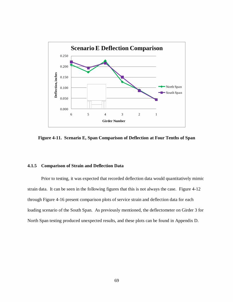
69

Figure 4-11. Scenario E, Span Comparison of Deflection at Four Tenths of Span

4.1.5 Comparison of Strain and Deflection Data

Prior to testing, it was expected that recorded deflection data would quantitatively mimic

strain data. It can be seen in the following figures that this is not always the case. Figure 4-12

through Figure 4-16 present comparison plots of service strain and deflection data for each

loading scenario of the South Span. As previously mentioned, the deflectometer on Girder 3 for

North Span testing produced unexpected results, and these plots can be found in Appendix D.

0.000

0.050

0.100

0.150

0.200

0.250

123456

Defl

ecti

on

, in

ch

es

Girder Number

Scenario E Deflection Comparison

North Span

South Span

70

Figure 4-12. South Span Scenario A Comparison of Strain and Deflection

Figure 4-13. South Span Scenario B Comparison of Strain and Deflection

0.000

0.050

0.100

0.150

0.200

0.250

0.300

0.350

0.0

10.0

20.0

30.0

40.0

50.0

60.0

70.0

80.0

123456

Defl

ecti

on

, in

ch

es

Str

ain

, m

icro

stra

in

Girder Number

South Span, Scenario A

Strain

Deflection

0.000

0.050

0.100

0.150

0.200

0.250

0.300

0.350

0.400

0.450

0.0

20.0

40.0

60.0

80.0

100.0

120.0

123456

Defl

ecti

on

, in

ch

es

Str

ain

, m

icro

stra

in

Girder Number

South Span, Scenario B

Strain

Deflection

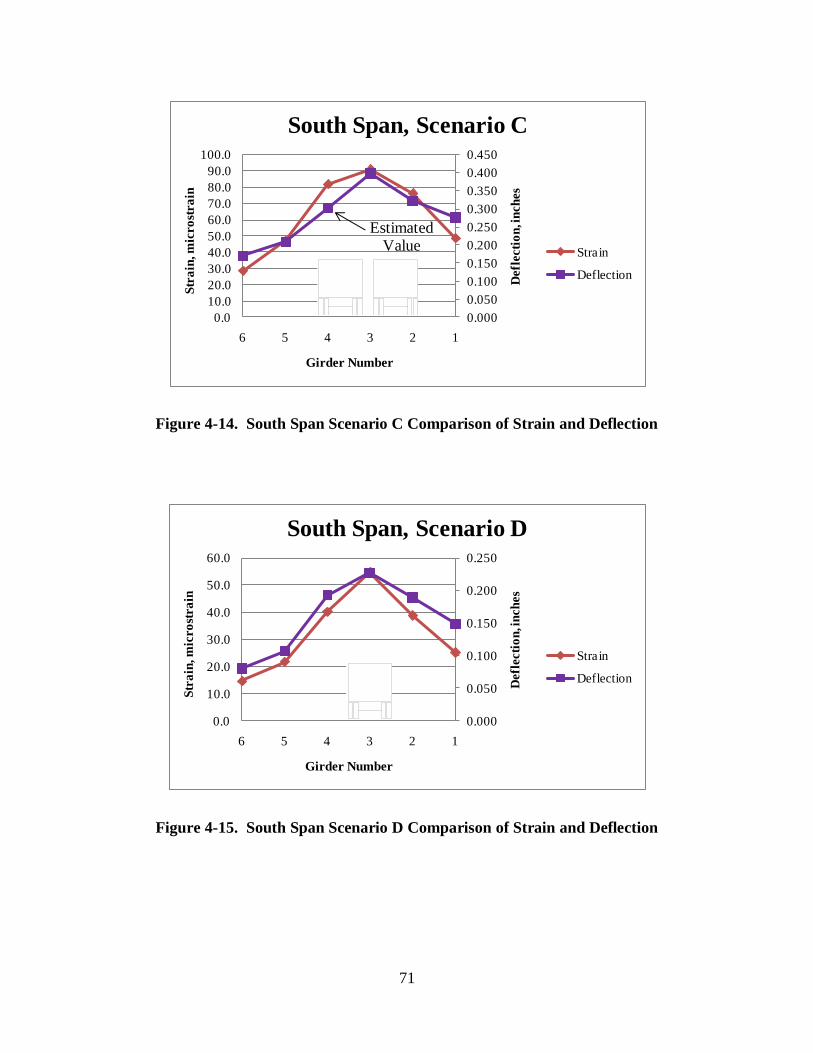
71

Figure 4-14. South Span Scenario C Comparison of Strain and Deflection

Figure 4-15. South Span Scenario D Comparison of Strain and Deflection

0.000

0.050

0.100

0.150

0.200

0.250

0.300

0.350

0.400

0.450

0.0

10.0

20.0

30.0

40.0

50.0

60.0

70.0

80.0

90.0

100.0

123456

Defl

ecti

on

, in

ch

es

Str

ain

, m

icro

stra

in

Girder Number

South Span, Scenario C

Strain

Deflection

Estimated Value

0.000

0.050

0.100

0.150

0.200

0.250

0.0

10.0

20.0

30.0

40.0

50.0

60.0

123456

Defl

ecti

on

, in

ch

es

Str

ain

, m

icro

stra

in

Girder Number

South Span, Scenario D

Strain

Deflection

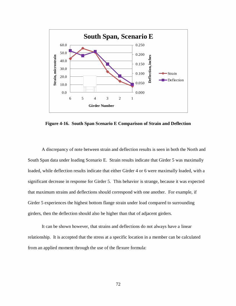
72

Figure 4-16. South Span Scenario E Comparison of Strain and Deflection

A discrepancy of note between strain and deflection results is seen in both the North and

South Span data under loading Scenario E. Strain results indicate that Girder 5 was maximally

loaded, while deflection results indicate that either Girder 4 or 6 were maximally loaded, with a

significant decrease in response for Girder 5. This behavior is strange, because it was expected

that maximum strains and deflections should correspond with one another. For example, if

Girder 5 experiences the highest bottom flange strain under load compared to surrounding

girders, then the deflection should also be higher than that of adjacent girders.

It can be shown however, that strains and deflections do not always have a linear

relationship. It is accepted that the stress at a specific location in a member can be calculated

from an applied moment through the use of the flexure formula:

0.000

0.050

0.100

0.150

0.200

0.250

0.0

10.0

20.0

30.0

40.0

50.0

60.0

123456

Defl

ecti

on

, in

ch

es

Str

ain

, m

icro

stra

in

Girder Number

South Span, Scenario E

Strain

Deflection

73

(4-1)

where σ is stress, M is the applied moment, y is the distance from the neutral axis to the location

for which stress is being calculated, and I is the moment of inertia of the member. Assuming

linear-elastic beam behavior under service loads, the relationship between stress and strain is

known, and the equation can be put in terms of strain, as follows:

(4-2)

where E is the member’s modulus of elasticity, ε is strain, and all other terms are as previously

defined. Solving Equation 4-2 for moment yields the following equations:

(4-3)

where all terms are as previously defined.

Using a simple span member under a single point load as an example, the maximum

moment is defined as:

(4-4)

where M is the moment, P is the point load, and L is the span of the member. Maximum

deflection in this case is given as:

(4-5)

74

where Δ is deflection, and all other variables are as previously defined. Inserting the maximum

moment equation into the maximum deflection equation produces the following:

(4-6)

where all variables have been defined previously. When Equation 4-5 is rearranged to solve for

moment, the following equation is produced:

(4-7)

where all variables are as previously defined. Combining Equations 4-3 and 4-7 and solving for

strain produces the following equation:

(4-8)

where all variables have been defined previously.

These equations show that the relationship between strain and deflection varies according

to the neutral axis depth of a section. Changing girder properties has an effect on the moment of

inertia of a section, and thus the neutral axis of that section. Because moment of inertia and

neutral axis depth do not vary linearly, strains and deflections of that section will not vary

linearly as properties change. This non-linear relationship between the strain and deflection of a

girder under the same applied moment, can cause the differences seen in the data. If two girders

have the same moment of inertia, but different neutral axis locations, under the same load

condition deflections would be similar, but strains could vary greatly. This difference could

75

possibly be seen between interior and exterior girders, where geometries vary greatly. It may

also be seen where cross bracing changes the properties of a girder by adding stiffness.

This behavior could also be attributed to loading differences between girders. Girders

directly beneath the loading trucks experience point loads, while adjacent girders experience

more of a distributed load. A girder loaded with a point load will not have the same deflection as

a girder under a distributed load, even if the applied moment on each girder is the same.

Although these are possible causes of differences in behavior between strain and deflection, the

exact cause is not fully understood.

Another difference between strain and deflection data can be seen on the South Span

under load Scenario B. This behavior was previously discussed in the comparison of service

strain data between the two spans. The North Span strain data, shown in Figure 4-3, as well as

all of the deflection data, presented in Figure 4-8, indicated that Girder 1 was maximally loaded.

Strain values recorded during testing of the South Span revealed that Girder 2 was maximally

loaded, as was intended in this load case. As previously discussed, one possible cause for this is

the difference in interior skew angle from obtuse to acute between the two spans. If the

difference in skew were the cause of this behavior it would be expected that the difference

between spans would be exhibited in deflection data as well. Although differences between

strains and deflections may be caused by changing girder properties, as mentioned above, the

cause of this discrepancy is not known.

As previously indicated, Girder 4 deflections were estimated for South Span testing under

load Scenario C using data from Girders 3 and 5, which can be seen in Figure 4-14. This causes

another slight discrepancy between the strain and deflection behavior, although the overall global

behavior in this case is shown to be very similar.

76

4.2 Service Strain Results at Center Support

Instrumentation located at the center support of the bridge on the bottom flange, top

flange, and concrete deck recorded strains during pseudo-static testing. As seen in Chapter 3, the

strain transducers were located in the same position for testing of both the North Span and the

South Span. Three unexpected behavioral events were observed during testing: differences

between North and South Span testing results, larger than expected differences in behavior as

load was applied from span to span, and bottom flange tension where compression was expected.

Because the instrumentation was left in place and loading was applied in the exact same

manner it was thought that all data from both days of testing would be similar and could be

analyzed together. This turned out not to be the case, and data from each day of testing is

presented separately. Some values are similar between the two days of testing, but others are

significantly different. The reason for this is not known, although a loss of adhesive bond

strength between transducer and bridge is suspected to be the reason. The transducers were left

in place between testing days, and the two part epoxy used to apply the transducers may have

lost some of its bond, causing discrepancies in the data between the two days of testing.

Similar to the previously presented service strains at four tenths of the span length, peak

values of service strains recorded at the center support of the bridge are presented here.

However, the behavior of continuous bridge girders at their center support creates multiple local

peaks in the data. For this reason, average peak data is presented when the load truck(s) are on

the North Span, near the center support, and on the South Span. These multiple locations of peak

values are labeled North, Center, and South in the following tables. An example of these three

peak value locations is shown in Figure 4-17, which presents bottom flange strains recorded at

the center support during a typical load test.

77

Figure 4-17. Bottom Flange Strain Peak Value Locations

The location of the instruments on the girder is signified by a B for bottom flange, T for

top flange, or C for concrete deck. All values are presented in microstrain, and the maximum

recorded value and standard deviation of the data are presented along with the average peak

value for each test. Also in the data tables is the number of tests performed for each scenario.

Loading Scenario E produced little to no response in the girders, and for this reason is omitted

from this presentation. Results of North Span testing are presented in Table 4-11 through Table

4-14, while South Span results are located in Table 4-15 through Table 4-18.

0 100 20040

30

20

10

0

10

20

Typical Bottom Flange Strain at Center Support

Truck Position Along Bridge, feet

Str

ain

, m

icro

stra

in

North

Peak

Center

Peak

South

Peak

78

Table 4-11. Scenario A, North Span Testing Center Support Strains

Load Location

Instrument Location B T C B T C B T C

Average -6.7 5.4 0.7 11.4 0.3 -5.7 -17.3 3.9 0.3

Maximum -7.2 6.0 2.0 13.4 1.0 -7.0 -18.0 5.0 1.0

Standard Deviation 0.6 0.5 1.2 1.8 0.6 1.5 0.7 0.9 0.6

Average -9.9 4.9 0.0 11.0 -1.0 0.0 -19.6 4.3 0.0

Maximum -11.0 5.0 0.0 12.2 -2.0 0.0 -20.2 5.0 0.0

Standard Deviation 1.0 0.1 0.0 1.1 1.0 0.0 0.7 0.6 0.0

Number of Tests

North Center South

Loading Scenario A, North Span Testing

Girder 1 Strains at Center Support (με)

Girder 2 Strains at Center Support (με)

3

Table 4-12. Scenario B, North Span Testing Center Support Strains

Load Location

Instrument Location B T C B T C B T C

Average -7.1 8.1 5.1 9.8 0.5 -2.8 -19.5 5.5 4.4

Maximum -8.7 9.0 6.0 10.9 1.0 -5.0 -22.0 6.0 6.0

Standard Deviation 1.2 0.7 1.2 1.5 0.6 2.2 1.8 1.0 1.5

Average -15.3 9.9 2.5 18.4 0.0 0.0 -32.3 8.4 0.0

Maximum -16.4 10.7 3.0 19.7 0.0 0.0 -32.8 8.7 0.0

Standard Deviation 0.8 0.7 0.6 0.9 0.0 0.0 0.4 0.3 0.0

Number of Tests

Loading Scenario B, North Span Testing

Girder 1 Strains at Center Support (με)

North Center South

Girder 2 Strains at Center Support (με)

4

79

Table 4-13. Scenario C, North Span Testing Center Support Strains

Load Location

Instrument Location B T C B T C B T C

Average -4.8 5.6 3.2 1.1 -0.3 -0.2 -6.8 4.0 2.8

Maximum -6.0 6.5 4.5 2.0 -1.0 -0.5 -8.0 5.0 4.0

Standard Deviation 1.0 0.8 1.1 0.9 1.0 0.6 0.9 1.2 1.1

Average -11.7 6.9 0.0 12.7 0.0 -3.3 -25.9 5.5 0.0

Maximum -12.5 7.5 0.0 13.8 -1.0 -4.0 -27.3 6.5 0.0

Standard Deviation 0.7 0.9 0.0 1.5 0.7 0.5 1.3 1.1 0.0

Number of Tests

Girder 2 Strains at Center Support (με)

Loading Scenario C, North Span Testing

Girder 1 Strains at Center Support (με)

North Center South

4

Table 4-14. Scenario D, North Span Testing Center Support Strains

Load Location

Instrument Location B T C B T C B T C

Average -2.8 3.1 1.8 0.6 0.5 -0.2 -2.1 2.6 1.6

Maximum -3.0 3.5 2.5 2.0 1.0 -0.5 -2.5 3.5 2.0

Standard Deviation 0.5 0.5 0.8 1.3 0.4 0.3 0.5 0.6 0.8

Average -4.7 4.3 0.0 5.1 1.1 0.0 -11.9 3.5 0.3

Maximum -6.0 5.0 0.0 5.9 1.5 0.0 -12.9 4.0 1.0

Standard Deviation 1.0 0.6 0.0 1.1 0.3 0.0 1.2 0.4 0.5

Number of Tests

Girder 2 Strains at Center Support (με)

North Center South

Loading Scenario D, North Span Testing

Girder 1 Strains at Center Support (με)

4

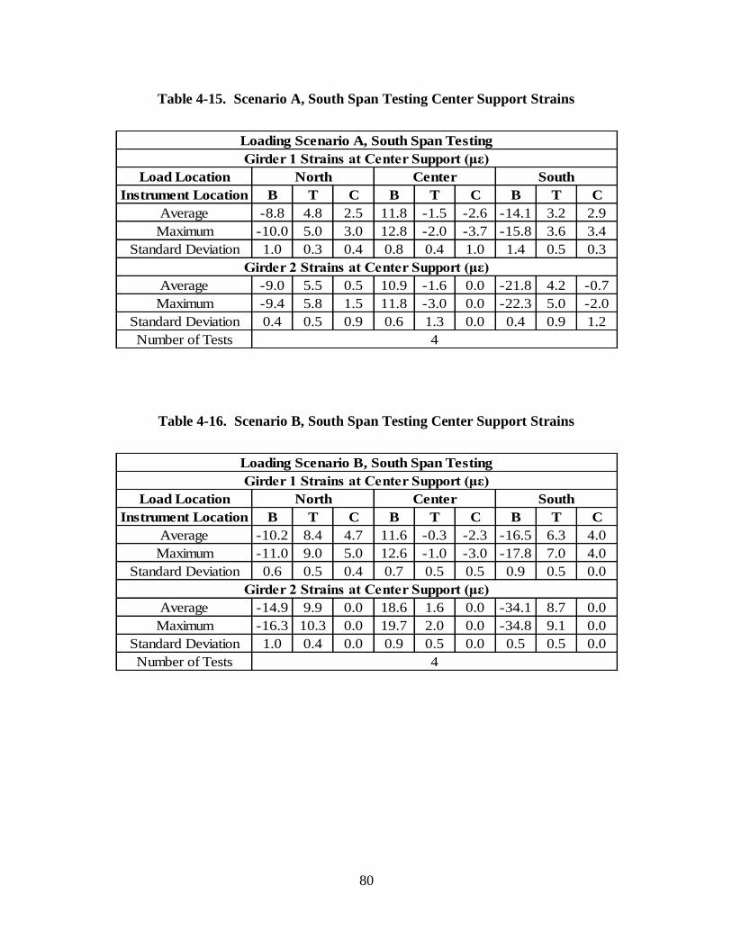
80

Table 4-15. Scenario A, South Span Testing Center Support Strains

Load Location

Instrument Location B T C B T C B T C

Average -8.8 4.8 2.5 11.8 -1.5 -2.6 -14.1 3.2 2.9

Maximum -10.0 5.0 3.0 12.8 -2.0 -3.7 -15.8 3.6 3.4

Standard Deviation 1.0 0.3 0.4 0.8 0.4 1.0 1.4 0.5 0.3

Average -9.0 5.5 0.5 10.9 -1.6 0.0 -21.8 4.2 -0.7

Maximum -9.4 5.8 1.5 11.8 -3.0 0.0 -22.3 5.0 -2.0

Standard Deviation 0.4 0.5 0.9 0.6 1.3 0.0 0.4 0.9 1.2

Number of Tests

Girder 2 Strains at Center Support (με)

Loading Scenario A, South Span Testing

Girder 1 Strains at Center Support (με)

North Center South

4

Table 4-16. Scenario B, South Span Testing Center Support Strains

Load Location

Instrument Location B T C B T C B T C

Average -10.2 8.4 4.7 11.6 -0.3 -2.3 -16.5 6.3 4.0

Maximum -11.0 9.0 5.0 12.6 -1.0 -3.0 -17.8 7.0 4.0

Standard Deviation 0.6 0.5 0.4 0.7 0.5 0.5 0.9 0.5 0.0

Average -14.9 9.9 0.0 18.6 1.6 0.0 -34.1 8.7 0.0

Maximum -16.3 10.3 0.0 19.7 2.0 0.0 -34.8 9.1 0.0

Standard Deviation 1.0 0.4 0.0 0.9 0.5 0.0 0.5 0.5 0.0

Number of Tests

Girder 2 Strains at Center Support (με)

South

Loading Scenario B, South Span Testing

Girder 1 Strains at Center Support (με)

North Center

4

81

Table 4-17. Scenario C, South Span Testing Center Support Strains

Load Location

Instrument Location B T C B T C B T C

Average -8.1 6.4 4.8 1.3 0.4 0.0 -5.9 4.5 2.8

Maximum -8.6 6.7 5.2 2.0 1.0 0.0 -6.3 4.8 3.2

Standard Deviation 0.4 0.3 0.4 0.5 0.5 0.0 0.4 0.4 0.4

Average -8.7 8.8 0.0 12.9 1.0 0.0 -24.6 7.4 0.0

Maximum -9.0 9.1 0.0 13.3 1.5 0.0 -25.1 7.7 0.0

Standard Deviation 0.2 0.3 0.0 0.4 0.4 0.0 0.5 0.3 0.0

Number of Tests

Loading Scenario C, South Span Testing

Girder 1 Strains at Center Support (με)

North Center South

Girder 2 Strains at Center Support (με)

4

Table 4-18. Scenario D, South Span Testing Center Support Strains

Load Location

Instrument Location B T C B T C B T C

Average -4.5 3.1 2.8 0.4 -0.1 0.4 -2.5 2.0 1.9

Maximum -5.0 3.5 3.2 1.0 -0.5 1.0 -3.0 2.3 2.8

Standard Deviation 0.4 0.5 0.4 0.5 0.3 0.5 0.4 0.6 0.9

Average -4.0 4.4 0.0 7.5 1.3 0.0 -14.4 3.7 0.0

Maximum -4.5 4.7 0.0 8.5 1.5 0.0 -15.5 3.9 0.0

Standard Deviation 0.7 0.3 0.0 0.8 0.3 0.0 0.8 0.2 0.0

Number of Tests

Girder 2 Strains at Center Support (με)

4

Loading Scenario D, South Span Testing

Girder 1 Strains at Center Support (με)

North Center South

By looking at this data, two of the three previously mentioned interesting events can be

seen to occur. The first is that the peak response that occurs when the load is applied to the

South Span is usually greater than that occurring on the North Span. This can be seen in Figure

4-18 which shows bottom flange strains recorded at the center support during a typical load test.

82

Figure 4-18. Bottom Flange Strain Peak Value Differences

As discussed in Chapter 3, due to the configuration of stiffeners and bracing at the center

support, strain transducers were offset 4 in. towards the north abutment instead of being

positioned at the exact center of the bridge. This location does not exhibit the symmetrical

behavior that would be expected if the instruments were located directly above the center

support. Figure 4-19 shows an influence line produced through a girder line analysis with a unit

load for a location offset 4 in. from the center support. It can be seen that on the North Span the

peak strains are slightly less than that on the South Span. This effect is thought to be amplified

by changes in differential girder stiffness due to different skew angles on the North and South

Spans, resulting in the differences in peak values seen in the data.

0 100 20040

30

20

10

0

10

20

Typical Bottom Flange Strain at Center Support

Truck Position Along Bridge, feet

Str

ain

, m

icro

stra

in

Difference in

Peak Values

83

Figure 4-19. Influence Line for Unit Load at Four Inches from Center Support

The second interesting phenomenon that can be seen is that the bottom flanges of both

girders are in tension when the load is near the center support. Due to the high bearing forces

acting at this location, this area of the bridge girder is considered to be a disturbed region. As a

disturbed region stress distributions are discontinuous and the strain profile in this area is

complex and non-linear. Because of this conventional beam theory does not apply. It was

expected, however, that the flange would be in compression due to the applied negative moment.

A comparison between expected and recorded behavior is presented in Figure 4-20. Expected

behavior is estimated with influence lines converted to strain through use of the flexure formula

presented in Equation 4-2. Experimental data presented are top and bottom flange strains

recorded at the center support during a typical test. It can be seen that the behavior of the top

flange compares well with the expected influence line behavior. The bottom flange behavior,

however, differs significantly from the expected influence line. This comparison shows that this

unexpected behavior is a local, and not a global, effect.

0 100 200

100

0

Influence Line at Four Inches from Center Support

Truck Position Along Bridge, feet

Mo

men

t, in

ch-k

ip

-155.7 -158.0

84

Figure 4-20. Expected versus Experimental Strain Values

This effect is possibly caused by local bearing stresses acting on the bottom flange. This

can be analyzed through the use of Hooke’s Law for homogenous isotropic materials in plane

stress, shown in the equations:

(4-9)

and

(4-10)

where σxx and σyy are stresses in the x and y-directions, E is the modulus of elasticity of the

material, ν is the Poisson’s ratio of the material, and εxx and εyy are strains in the x and y-

directions, respectively (Boresi 2003). For this bridge the x-direction is oriented longitudinally,

while stresses in the y-direction occur vertically, as depicted in Figure 4-21.

0 100 20060

40

20

0

Bottom Flange IL

Top Flange IL

Bottom Flange Exp.

Top Flange Exp .

Influence Lines vs. Experimental Data

Truck Position Along Bridge, feet

Str

ain

, m

icro

stra

in

85

Figure 4-21. Sign Convention at Center Support

When these equations are used together, it can be shown that, due to Poisson’s effect,

vertical compressive stresses can cause longitudinal tension strains on the bottom flange. As the

moment in the girder decreases near midspan, the ratio of shear force, which creates the bearing

stress, to moment increases, and this bearing induced tension strain can overcome the

compressive strain caused by bending. This can be seen in Figure 4-22, where strain in the

bottom flange is presented as a function of the ratio of shear to moment acting at the center

support. Values used to calculate stresses were determined from the dimensions of the girder at

the center support. Because the true moment of inertia of the girder is unknown due to the

effects of bearing stiffeners and cross-bracing present at this location, this value was varied in the

plot. The moment of inertia, I, was calculated with a transformed section analysis neglecting all

stiffeners and bracing. It can be seen that as the moment of inertia increases, the strain in the x-

direction reaches tension at smaller ratios of shear to moment.

North Span South Span

y

x

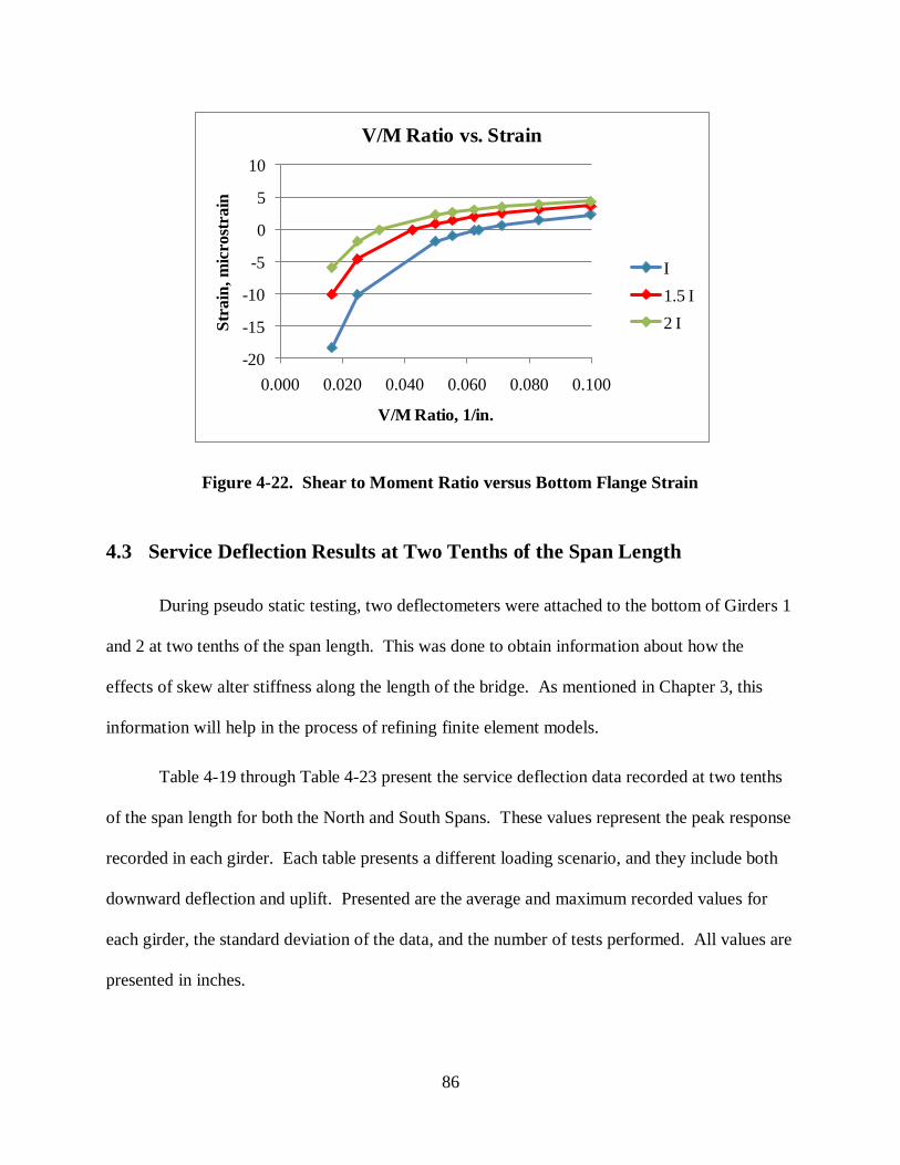
86

Figure 4-22. Shear to Moment Ratio versus Bottom Flange Strain

4.3 Service Deflection Results at Two Tenths of the Span Length

During pseudo static testing, two deflectometers were attached to the bottom of Girders 1

and 2 at two tenths of the span length. This was done to obtain information about how the

effects of skew alter stiffness along the length of the bridge. As mentioned in Chapter 3, this

information will help in the process of refining finite element models.

Table 4-19 through Table 4-23 present the service deflection data recorded at two tenths

of the span length for both the North and South Spans. These values represent the peak response

recorded in each girder. Each table presents a different loading scenario, and they include both

downward deflection and uplift. Presented are the average and maximum recorded values for

each girder, the standard deviation of the data, and the number of tests performed. All values are

presented in inches.

-20

-15

-10

-5

0

5

10

0.000 0.020 0.040 0.060 0.080 0.100

Str

ain

, m

icro

stra

in

V/M Ratio, 1/in.

V/M Ratio vs. Strain

I

1.5 I

2 I

87

Table 4-19. Two Tenths Service Deflections, Scenario A

1 2 1 2

0.222 0.127 0.201 0.178

0.223 0.128 0.204 0.181

0.002 0.002 0.003 0.002

-0.074 -0.048 -0.079 -0.067

-0.076 -0.050 -0.083 -0.069

0.003 0.002 0.004 0.003

Average

Maximum

Standard Deviation

Maximum

Standard Deviation

Uplift Deflection (in)

Average

Number of Tests 3 4

Loading Scenario A

Downward Deflection (in)

Girder Number

Span North South

Table 4-20. Two Tenths Service Deflections, Scenario B

1 2 1 2

0.308 0.191 0.257 0.300

0.311 0.194 0.263 0.306

0.003 0.002 0.004 0.005

-0.122 -0.085 -0.119 -0.109

-0.123 -0.086 -0.122 -0.111

0.002 0.001 0.002 0.001

Span North South

Average

Maximum

Standard Deviation

Uplift Deflection (in)

Average

Maximum

Standard Deviation

Number of Tests 4 4

Girder Number

Loading Scenario B

Downward Deflection (in)

88

Table 4-21. Two Tenths Service Deflections, Scenario C

1 2 1 2

0.194 0.164 0.167 0.232

0.200 0.166 0.170 0.238

0.005 0.002 0.003 0.005

-0.098 -0.076 -0.090 -0.090

-0.100 -0.077 -0.094 -0.094

0.002 0.001 0.003 0.003Standard Deviation

Uplift Deflection (in)

Average

Average

Maximum

Standard Deviation

Maximum

Downward Deflection (in)

Girder Number

Span North South

Loading Scenario C

Number of Tests 4 4

Table 4-22. Two Tenths Service Deflections, Scenario D

1 2 1 2

0.098 0.100 0.094 0.128

0.098 0.101 0.095 0.129

0.001 0.001 0.001 0.001

-0.050 -0.039 -0.051 -0.050

-0.051 -0.040 -0.054 -0.052

0.001 0.001 0.002 0.002

Span North South

Average

Maximum

Loading Scenario D

Downward Deflection (in)

Number of Tests 4 4

Standard Deviation

Girder Number

Standard Deviation

Uplift Deflection (in)

Average

Maximum

89

Table 4-23. Two Tenths Service Deflections, Scenario E

1 2 1 2

0.026 0.051 0.022 0.057

0.028 0.053 0.024 0.059

0.002 0.002 0.001 0.002

-0.022 -0.029 -0.020 -0.033

-0.023 -0.030 -0.023 -0.041

0.001 0.000 0.003 0.006

Maximum

Standard Deviation

Average

Maximum

Standard Deviation

Uplift Deflection (in)

Average

Downward Deflection (in)

Girder Number

Span North South

Loading Scenario E

Number of Tests 4 4

Comparing this deflection data with that recorded under the same loading conditions at

four tenths of the span length, it is expected that exhibited behavior would be similar, but of a

lesser magnitude. South Span deflections behave as expected, with deflections at two tenths of

the span length following the behavioral pattern of those at four tenths of the span length.

Deflections recorded on the North Span, however, exhibit unexpected behavior, especially in

loading Scenarios B through D. This behavior is identified in Figure 4-23, which presents the

peak downward deflection of each girder under loading Scenario C.

90

Figure 4-23. Scenario C Deflection Comparison

It was thought that this behavior may have only been evident when examining peak

values for each girder because of the offset of peak values between the girders. However, when

the deflections of each girder were examined at the same points in time there was only a

negligible change in values, and this behavior was still observed. Figure 4-24 shows deflections

at two tenths of the span length for a typical test. It can be seen that Girder 2 reaches peak

deflection before Girder 1 does. The deflection of Girder 1 at this point in time, however, is only

slightly lower than the peak value recorded. This is also true for Girder 2 at the time of peak

deflection for Girder 1.

0.000

0.050

0.100

0.150

0.200

0.250

0.300

0.350

0.400

0.450

123456

Defl

ecti

on

, in

ch

es

Girder Number

Scenario C Deflection Comparison

North Span Four Tenths

South Span Four Tenths

North Span Two Tenths

South Span Two Tenths

Expected

Unexpected

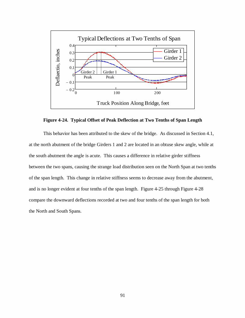
91

Figure 4-24. Typical Offset of Peak Deflection at Two Tenths of Span Length

This behavior has been attributed to the skew of the bridge. As discussed in Section 4.1,

at the north abutment of the bridge Girders 1 and 2 are located in an obtuse skew angle, while at

the south abutment the angle is acute. This causes a difference in relative girder stiffness

between the two spans, causing the strange load distribution seen on the North Span at two tenths

of the span length. This change in relative stiffness seems to decrease away from the abutment,

and is no longer evident at four tenths of the span length. Figure 4-25 through Figure 4-28

compare the downward deflections recorded at two and four tenths of the span length for both

the North and South Spans.

0 100 2000.2

0.1

0

0.1

0.2

0.3

0.4

Girder 1

Girder 2

Typical Deflections at Two Tenths of Span

Truck Position Along Bridge, feet

Def

laec

tio, in

ches

Girder 1

Peak

Girder 2

Peak

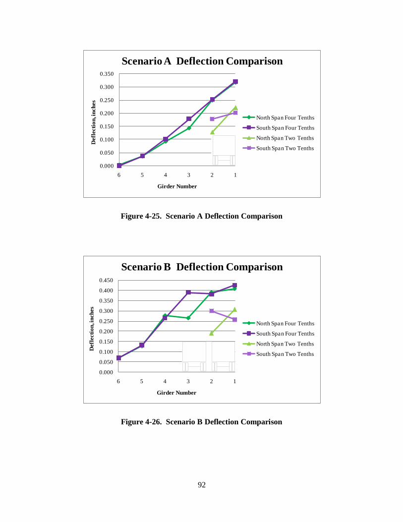
92

Figure 4-25. Scenario A Deflection Comparison

Figure 4-26. Scenario B Deflection Comparison

0.000

0.050

0.100

0.150

0.200

0.250

0.300

0.350

123456

Defl

ecti

on

, in

ch

es

Girder Number

Scenario A Deflection Comparison

North Span Four Tenths

South Span Four Tenths

North Span Two Tenths

South Span Two Tenths

0.000

0.050

0.100

0.150

0.200

0.250

0.300

0.350

0.400

0.450

123456

Defl

ecti

on

, in

ch

es

Girder Number

Scenario B Deflection Comparison

North Span Four Tenths

South Span Four Tenths

North Span Two Tenths

South Span Two Tenths

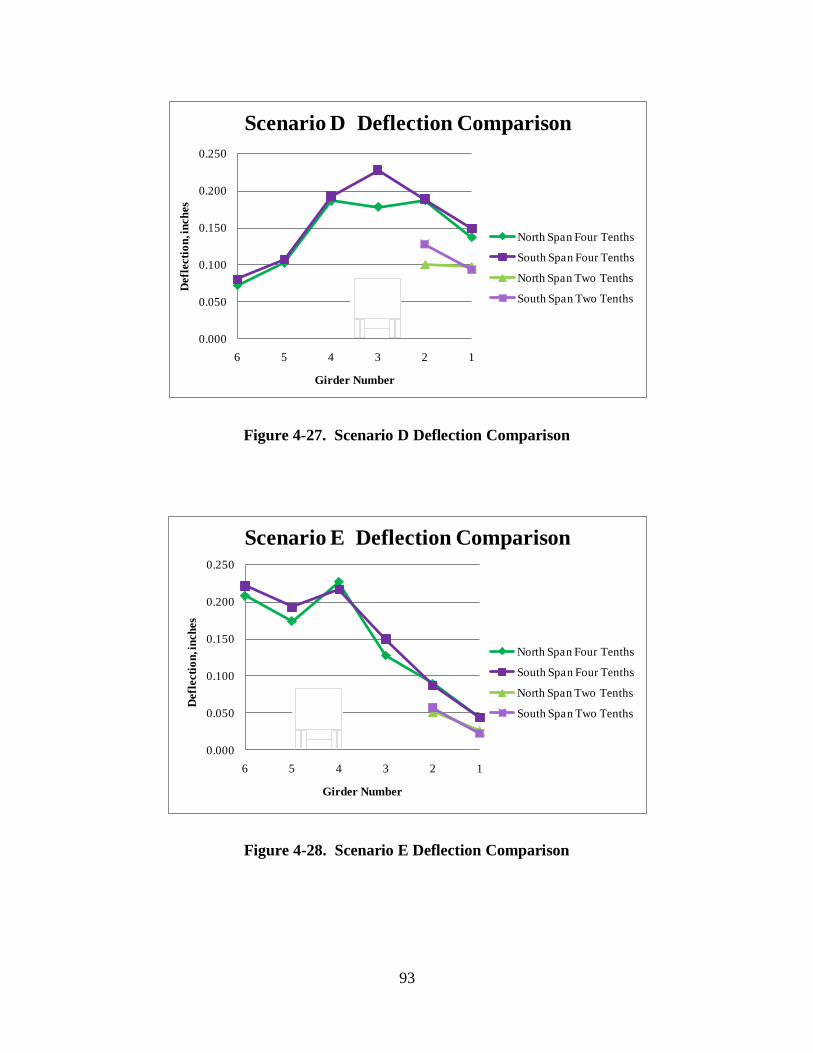
93

Figure 4-27. Scenario D Deflection Comparison

Figure 4-28. Scenario E Deflection Comparison

0.000

0.050

0.100

0.150

0.200

0.250

123456

Defl

ecti

on

, in

ch

es

Girder Number

Scenario D Deflection Comparison

North Span Four Tenths

South Span Four Tenths

North Span Two Tenths

South Span Two Tenths

0.000

0.050

0.100

0.150

0.200

0.250

123456

Defl

ecti

on

, in

ch

es

Girder Number

Scenario E Deflection Comparison

North Span Four Tenths

South Span Four Tenths

North Span Two Tenths

South Span Two Tenths

94

4.4 Load Distribution Results

4.4.1 AASHTO Load Distribution Factors

As discussed in Section 2.2, AASHTO presents equations to calculate bending moment

distribution factors for use in the design process. These equations were used to calculate the

distribution factors shown in Table 4-24 4-24. The calculations using these equations are

presented in Appendix E. When determining the distribution factor for an exterior girder it is

necessary to use the lever rule. The details of this are presented in Appendix F. Cross sectional

properties at four tenths of the span length were used to calculate these values.

To take into account the effects of bridge skew on load distribution, AASHTO presents

equations that reduce calculated distribution factors. These equations are presented in Section

2.2, and are only applicable for bridges with skew angles between 30 and 60 degrees. With a

skew of 17 degrees, the Route 15 bridge does not meet the criteria to apply distribution factor

reduction. However, because effects of skew were observed during testing, the AASHTO

distribution factor reduction equations have been used for comparison purposes. Using

equations 2-6 and 2-7, a reduction of 1.1 per cent was calculated and applied to all distribution

factors. The skew reduced distribution factors can also be seen in Table 4-24.

Table 4-24. AASHTO Load Distribution Factors

Girder:Lanes

Loaded

Distribution

Factors

Skew Reduced

D.F.

Interior 1 0.357 0.353

Interior 2+ 0.577 0.570

Exterior 1 0.493 0.488

Exterior 2+ 0.481 0.407

AASHTO Distribution Factors

95

4.4.2 Procedure for Calculating Experimental Load Distribution Factors

Load distribution factors, as discussed in Chapter 3, can be calculated from strain and

deflection data recorded during live load testing. Test data can be used to calculate a distribution

factor for the girder that has the largest response relative to all other girders for a single test.

Responses for all girders are taken at the same point in time that the peak response occurs for the

maximally loaded girder. A distribution factor is then calculated through the use of the

following equation:

(4-11)

where gmax is the distribution factor of the maximally loaded girder, Rmax is the recorded response

of the maximally loaded girder, n is the number of trucks applying load, m is the total number of

girders, and Rj is the recorded response in the jth girder at the time of the maximum response.

To observe the effects of skew on distribution factors, Equation 4-11 is altered slightly to

give the following equation:

(4-12)

where Rpeakj is the peak response recorded in the jth girder, and all other variables are as

previously defined.

4.4.3 Strain and Deflection Distribution Results

Although similar to data presented in Section 4.1, the strain and deflection values used to

calculate distribution factors are not the peak values for each girder. As stated above, response

96

values are taken for all girders at the point in time when the peak response occurs in the

maximally loaded girder. Responses recorded when the loading truck(s) were located on the

opposite span, which caused uplift and compression in bottom flanges, were not used to calculate

distribution factors. The average distribution values for both strain and compression of each

span can be found in Appendix G, along with the maximum values and standard deviation of the

data.

As discussed in Section 4.1.5, the deflection value presented for Girder 4 under loading

Scenario C on the South Span has been approximated by averaging adjacent values. Girder 3

deflection values from North Span testing are once again suspect, but as before are presented as

recorded. This did have an effect on distribution factors, as Girder 3 should have experienced

the maximum response under certain loading conditions. For these situations, distribution

factors have been calculated for the girder exhibiting maximum response and Girder 3.

4.4.4 Distribution Factors Calculated from Experimental Data

The following tables present load distribution factors calculated from experimental data.

Moment distribution factors were calculated using both the distribution data presented above, as

well as the service data presented in Section 4.1. Distribution data is used in Equation 4-11,

while service data is used in Equation 4-12. As previously mentioned, the use of service data,

which represents the peak values for each individual girder, shows the effect of skew on load

distribution through the offset of peak girder response. This offset is seen in Figure 4-29, which

presents bottom flange strains of each girder on a typical test.

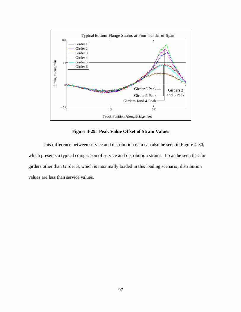
97

Figure 4-29. Peak Value Offset of Strain Values

This difference between service and distribution data can also be seen in Figure 4-30,

which presents a typical comparison of service and distribution strains. It can be seen that for

girders other than Girder 3, which is maximally loaded in this loading scenario, distribution

values are less than service values.

0 100 20050

0

50

100

Girder 1

Girder 2

Girder 3

Girder 4

Girder 5

Girder 6

Typical Bottom Flange Strains at Four Tenths of Span

Truck Position Along Bridge, feet

Str

ain

, m

icro

stra

in

Girder 6 Peak Girders 2

and 3 Peak

Girders 1and 4 Peak

Girder 5 Peak

98

Figure 4-30. Comparison of Service and Distribution Strain Data

Distribution factors calculated using the distribution data are labeled D. F., and those

calculated using service data are labeled Skew D. F. The reduction of distribution factors due to

skew effects has been calculated as a percentage and is presented as well. Because strain and

deflection data sometimes conflicted as to which girder experienced maximum load, the girder

for which distribution factors were calculated is labeled. Table 4-25 presents distribution factors

calculated from North Span data, while Table 4-26 presents those calculated using data collected

during testing of the South Span.

0.0

10.0

20.0

30.0

40.0

50.0

60.0

70.0

80.0

90.0

100.0

123456

Str

ain

, m

icro

stra

in

Girder Number

Typical Service vs. Distribution Strain

Service

Distribution

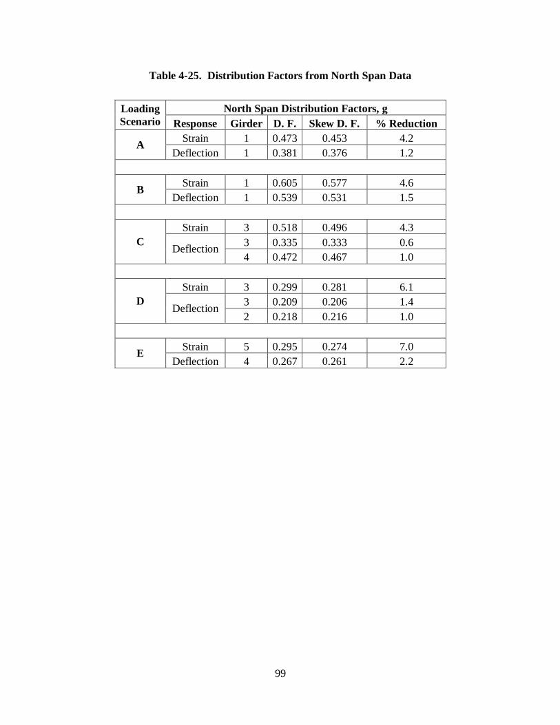
99

Table 4-25. Distribution Factors from North Span Data

Loading

Scenario

North Span Distribution Factors, g

Response Girder D. F. Skew D. F. % Reduction

A Strain 1 0.473 0.453 4.2

Deflection 1 0.381 0.376 1.2

B Strain 1 0.605 0.577 4.6

Deflection 1 0.539 0.531 1.5

C

Strain 3 0.518 0.496 4.3

Deflection 3 0.335 0.333 0.6

4 0.472 0.467 1.0

D

Strain 3 0.299 0.281 6.1

Deflection 3 0.209 0.206 1.4

2 0.218 0.216 1.0

E Strain 5 0.295 0.274 7.0

Deflection 4 0.267 0.261 2.2

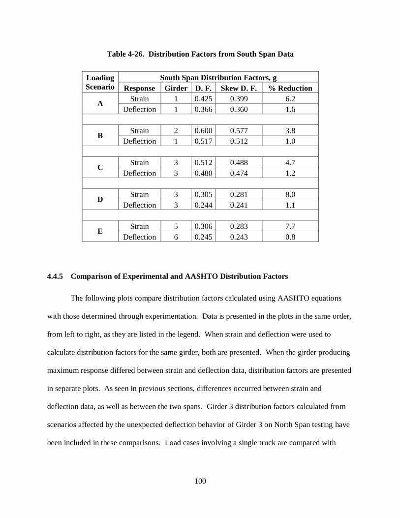
100

Table 4-26. Distribution Factors from South Span Data

Loading

Scenario

South Span Distribution Factors, g

Response Girder D. F. Skew D. F. % Reduction

A Strain 1 0.425 0.399 6.2

Deflection 1 0.366 0.360 1.6

B Strain 2 0.600 0.577 3.8

Deflection 1 0.517 0.512 1.0

C Strain 3 0.512 0.488 4.7

Deflection 3 0.480 0.474 1.2

D Strain 3 0.305 0.281 8.0

Deflection 3 0.244 0.241 1.1

E Strain 5 0.306 0.283 7.7

Deflection 6 0.245 0.243 0.8

4.4.5 Comparison of Experimental and AASHTO Distribution Factors

The following plots compare distribution factors calculated using AASHTO equations

with those determined through experimentation. Data is presented in the plots in the same order,

from left to right, as they are listed in the legend. When strain and deflection were used to

calculate distribution factors for the same girder, both are presented. When the girder producing

maximum response differed between strain and deflection data, distribution factors are presented

in separate plots. As seen in previous sections, differences occurred between strain and

deflection data, as well as between the two spans. Girder 3 distribution factors calculated from

scenarios affected by the unexpected deflection behavior of Girder 3 on North Span testing have

been included in these comparisons. Load cases involving a single truck are compared with

101

AASHTO one lane loaded distribution factors, while those involving two loading trucks are

compared with factors calculated using equations designed for two or more lanes loaded.

Experimentally derived distribution factors for Girder 1 under loading Scenario A are

presented in Figure 4-31. These values are compared with the AASHTO distribution factor

calculated for exterior girders with one lane loaded. It can be seen that the AASHTO equation

produces a greater, and therefore more conservative, distribution factor than those determined

experimentally. It can also be seen that distribution factors determined using strain data are more

conservative than those using deflection data.

Figure 4-31. Distribution Factor Comparison, Scenario A Girder 1

Figure 4-32 and Figure 4-33 show distribution factors calculated from load Scenario B

testing. Other than strain values for South Span testing all data resulted in Girder 1 being the

maximally loaded girder. Girder 2 was the girder with the largest recorded strain on the South

Span. The distribution factors were compared with the AASHTO distribution factor calculated

0.4930.473

0.381

0.425

0.366

0

0.1

0.2

0.3

0.4

0.5

0.6

Dis

trib

uti

on

Fa

cto

r, g

Distribution Factors, Scenario A, Girder 1

AASHTO

North Strain

North Deflection

South Strain

South Deflection

102

for an exterior girder with two or more lanes loaded. The distribution factor for Girder 2,

calculated from strain values recorded during South Span testing, is compared with the

AASHTO distribution factor for an interior girder with two or more lanes loaded and with a

distribution factor calculated using the lever rule. For both interior and exterior girders under

loading Scenario B, it can be seen that the AASHTO equations are un-conservative compared

with experimental data. The lever rule presents an upper bound for the distribution factor for

Girder 2. This value is conservative compared to the distribution factor calculated using

experimental data. Strain data once again appears to be conservative compared with deflection

data. Comparing Figure 4-31 and Figure 4-32 it is also interesting to note that AASHTO

distribution factor calculations predict a decrease from values for one lane loaded to two lanes

loaded, while experimentally determined distribution factors increase.

Figure 4-32. Distribution Factor Comparison, Scenario B Girder 1

0.411

0.605

0.5390.517

0

0.1

0.2

0.3

0.4

0.5

0.6

0.7

Dis

trib

uti

on

Fa

cto

r, g

Distribution Factors, Scenario B, Girder 1

AASHTO

North Strain

North Deflection

South Deflection

103

Figure 4-33. Distribution Factor Comparison, Scenario B Girder 2

Figure 4-34 presents the comparison of load distribution factors calculated from data

obtained during loading Scenario C. This scenario was intended to maximally load Girder 3,

which it did for all cases other than deflection on the North Span. As previously mentioned, that

unexpected deflection data was used to calculate a distribution factor for Girder 3, even though it

was not the maximally loaded girder. This behavior is the cause of the low distribution factor

presented. Experimental factors are compared with the AASHTO factor calculated using

equations designed for interior girders with two or more lanes loaded. Factors calculated from

strain data for each span are very similar, and show much more distribution of load than the

AASHTO factor would indicate.

0.577

0.828

0.600

0

0.1

0.2

0.3

0.4

0.5

0.6

0.7

0.8

0.9

Dis

trib

uti

on

Fa

cto

r, g

Distribution Factors, Scenario B, Girder 2

AASHTO

Lever Rule

South Strain

104

Figure 4-34. Distribution Factor Comparison, Scenario C Girder 3

As seen in the presentation of distribution factors calculated from data obtained during

loading Scenario D, which is shown in Figure 4-35, North Span deflection data produced a much

lower distribution factor than all other cases. Comparisons are made with the AASHTO value

calculated for interior girders with one lane loaded. It can be seen that the AASHTO equation is

once again conservative compared with experimental data, and that factors calculated from strain

data seem to be conservative compared with those calculated from deflection data.

0.577

0.518

0.335

0.5120.480

0

0.1

0.2

0.3

0.4

0.5

0.6

0.7

Dis

trib

uti

on

Fa

cto

r, g

Distribution Factors, Scenario C, Girder 3

AASHTO

North Strain

North Deflection

South Strain

South Deflection

105

Figure 4-35. Distribution Factor Comparison, Scenario D Girder 3

Figure 4-36 through Figure 4-38 present distribution factors calculated from test data

recorded during load Scenario E. This scenario placed a load truck in the center of the left traffic

lane, and was expected to maximally load either Girder 4 or 5. On each span, strain values

indicated that Girder 5 was maximally loaded, and distribution factors were calculated

accordingly. However, this was not the case for deflection data. For both spans, deflection data

indicated that deflections for Girder 5 were less than those for Girders 4 and 6. This appears to

be an instrumentation error, similar to that with Girder 3 in the North Span data, but it appears

that the deflectometer produced good quality data for all other testing scenarios. Because there is

no reason to discount this data, other than the fact that is was unexpected and differs from the

behavior characterized by the strain data, distribution factors are presented for Girders 4 and 6,

which were the maximally loaded girders for the North and South Span testing, respectively.

0.357

0.299

0.209

0.305

0.244

0

0.05

0.1

0.15

0.2

0.25

0.3

0.35

0.4

Dis

trib

uti

on

Fa

cto

r, g

Distribution Factors, Scenario D, Girder 3

AASHTO

North Strain

North Deflection

South Strain

South Deflection

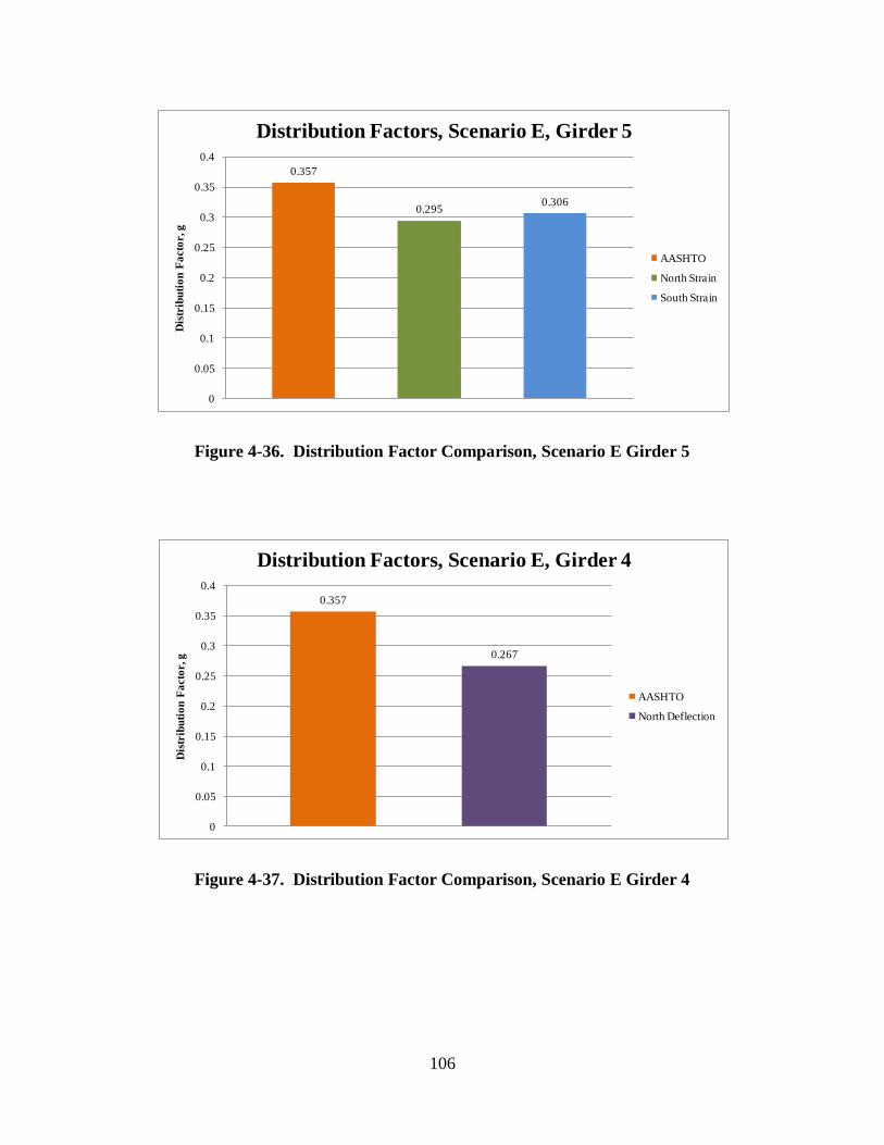
106

Figure 4-36. Distribution Factor Comparison, Scenario E Girder 5

Figure 4-37. Distribution Factor Comparison, Scenario E Girder 4

0.357

0.2950.306

0

0.05

0.1

0.15

0.2

0.25

0.3

0.35

0.4

Dis

trib

uti

on

Fa

cto

r, g

Distribution Factors, Scenario E, Girder 5

AASHTO

North Strain

South Strain

0.357

0.267

0

0.05

0.1

0.15

0.2

0.25

0.3

0.35

0.4

Dis

trib

uti

on

Fa

cto

r, g

Distribution Factors, Scenario E, Girder 4

AASHTO

North Deflection

107

Figure 4-38. Distribution Factor Comparison, Scenario E Girder 6

4.4.6 Skew Effects on Distribution Factors

As previously discussed, distribution factors calculated from peak values for all girders,

as opposed to values at the point of peak response for the maximally loaded girder, presents the

effect of skew on load distribution. As noted by AASHTO, bridges with skew have better

distribution of load, and thus reduced distribution factors, than non-skewed bridges. The

reduction of load distribution factors is presented in comparison with the reduction applied

through the use of AASHTO equations in Figure 4-39 through Figure 4-44. Because of the

previously mentioned discrepancies present in the deflection data, distribution factors calculated

from deflection data are only included in these plots if they correspond with those calculated

from strain data. For load Scenario B, where strain data was not consistent between spans,

reductions of distribution factors are presented for Girders 5 and 6.

0.577

0.245

0

0.1

0.2

0.3

0.4

0.5

0.6

0.7

Dis

trib

uti

on

Fa

cto

r, g

Distribution Factors, Scenario E, Girder 6

AASHTO

South Deflection

108

Reductions in distribution factors calculated from strain results varied from 3.8 to 8.0 per

cent, while those calculated from deflection results ranged from 0.8 to 2.2 per cent. These values

can be compared with the 1.1 per cent reduction applied to AASHTO distribution factors.

Figure 4-39. Skew Effect on Distribution Factors, Scenario A Girder 1

Figure 4-40. Skew Effect on Distribution Factors, Scenario B Girder 1

0.4930.4880.473

0.453

0.3810.376

0.4250.399

0.3660.360

0

0.1

0.2

0.3

0.4

0.5

0.6

Dis

trib

uti

on

Fa

cto

r, g

Skew Reduced Distribution Factors

Scenario A, Girder 1

AASHTO

AASHTO Skew

North Strain

North Strain Skew

North Deflection

North Deflection Skew

South Strain

South Strain Skew

South Deflection

South Deflection Skew

0.411 0.407

0.6050.577

0.539 0.531 0.517 0.512

0

0.1

0.2

0.3

0.4

0.5

0.6

0.7

Dis

trib

uti

on

Fa

cto

r, g

Skew Reduced Distribution Factors

Scenario B, Girder 1

AASHTO

AASHTO Skew

North Strain

North Strain Skew

North Deflection

North Deflection Skew

South Deflection

South Deflection Skew

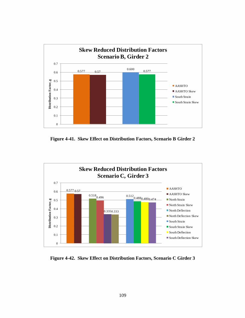
109

Figure 4-41. Skew Effect on Distribution Factors, Scenario B Girder 2

Figure 4-42. Skew Effect on Distribution Factors, Scenario C Girder 3

0.577 0.570.600

0.577

0

0.1

0.2

0.3

0.4

0.5

0.6

0.7

Dis

trib

uti

on

Fa

cto

r, g

Skew Reduced Distribution Factors

Scenario B, Girder 2

AASHTO

AASHTO Skew

South Strain

South Strain Skew

0.577 0.57

0.5180.496

0.3350.333

0.5120.4880.4800.474

0

0.1

0.2

0.3

0.4

0.5

0.6

0.7

Dis

trib

uti

on

Fa

cto

r, g

Skew Reduced Distribution Factors

Scenario C, Girder 3

AASHTO

AASHTO Skew

North Strain

North Strain Skew

North Deflection

North Deflection Skew

South Strain

South Strain Skew

South Deflection

South Deflection Skew

110

Figure 4-43. Skew Effect on Distribution Factors, Scenario D Girder 3

Figure 4-44. Skew Effect on Distribution Factors, Scenario E Girder 5

0.3570.353

0.2990.281

0.2090.206

0.305

0.281

0.2440.241

0

0.05

0.1

0.15

0.2

0.25

0.3

0.35

0.4D

istr

ibu

tio

n F

acto

r, g

Skew Reduced Distribution Factors

Scenario D, Girder 3

AASHTO

AASHTO Skew

North Strain

North Strain Skew

North Deflection

North Deflection Skew

South Strain

South Strain Skew

South Deflection

South Deflection Skew

0.357 0.353

0.2950.274

0.3060.283

0

0.05

0.1

0.15

0.2

0.25

0.3

0.35

0.4

Dis

trib

uti

on

Fa

cto

r, g

Skew Reduced Distribution Factors

Scenario E, Girder 5

AASHTO

AASHTO Skew

North Strain

North Strain Skew

South Strain

South Strain Skew

111

4.5 Dynamic Load Allowance Results

4.5.1 Procedure for Calculating Experimental Dynamic Load Allowance

Dynamic load allowance, as discussed in Chapter 3, can be calculated from strain and

deflection data recorded during live load testing. Comparing peak values recorded during

pseudo-static testing with those recorded during highway speed testing display the increase in

girder response created by dynamic effects. This increase in response is quantified and presented

as dynamic load allowance, or impact factor, through the use of the following equation:

(4-13)

where IM is the dynamic load allowance, Rdyn is the peak dynamic response, and Rstat is the peak

static response.

4.5.2 Dynamic Load Allowance Results

In order to properly calculate dynamic load allowance from experimental data, it is

important that the pseudo-static and highway speed loading trucks are applied in the exact same

location. Unfortunately for these tests, the truck drivers had difficulty staying in the center of the

travel lane during highway speed tests. At the time of testing it was thought that this mistake

would only create small errors in the results. This proved to not be the case, as many girders

experienced a smaller response under dynamic loading than under pseudo-static loading,

indicating negative impact factors. Dynamic load allowance is usually calculated with dynamic

data recorded while trucks travel at much faster speeds. As discussed in Chapter 3, due to the

112

limited approach 25 miles per hour was the top speed attainable, which also contributed to the

condition of the dynamic load allowance results.

Due to the poor results, this data does not aid in the characterization of bridge

performance and is not presented here. This data can be found in Appendix H if needed for

comparison purposes with future live load test results. All results were recorded under loading

Scenario D, with the load truck in the right travel lane. Using this data along with service data

recorded during pseudo-static testing under loading Scenario D, which was presented in Section

4.1, impact factors were calculated through the use of equation 4-2. If no errors had occurred

during testing, calculated dynamic load allowance values would be compared with IM = 0.33

from AASHTO Specification Table 3.6.2.1-1. Dynamic load allowance values calculated from

both strain and deflection response can also be found in Appendix H.

4.6 Neutral Axis Analysis Results

As described in Chapter 3, multiple strain transducers were installed on select girders to

capture the vertical strain profile created under loading. Three strain transducers installed on the

bottom and top flange and either on the bottom of the concrete deck, or on the web 12 in. above

the bottom flange, were expected to yield results indicating the location of the composite girder’s

neutral axis. Girders 1, 2, and 3 were instrumented with multiple strain transducers at four tenths

of the span length, along with Girders 1 and 2 at the center support. As discussed in Chapter 2,

the location of the neutral axis is an indication of the amount of composite action occurring

between the steel girder and the concrete deck. By comparing the location of the neutral axis

derived from experimental results with that determined through a classical transformed section

analysis, the percentage of composite action can be determined.

113

Other factors can also influence the location of the neutral axis of a composite girder.

Concrete delamination on the deck will reduce the area of the deck available for compression,

thus lowering the neutral axis of the section. Cross bracing connected to a girder can also add

stiffness and change the neutral axis location of a section. For this presentation all differences

between theoretical and experimental measurements of the neutral axis location will be attributed

to loss of composite action. Comparisons with future live load, non-destructive, and materials

testing will reveal the true cause of changes in neutral axis location.

4.6.1 Theoretical Neutral Axis Calculations

The neutral axis of a girder in bending is located at the depth of the cross section where

no bending stresses occur. A composite section’s neutral axis can be found using the

transformed section method. In the transformed section method the concrete deck is transformed

into an equivalent amount of steel using the modular ratio, n, of the two materials. The modular

ratio is dependent on the Modulus of Elasticity of concrete, which is not precisely known. For

the purposes of this analysis, three different values were used. The first value used is 3605 ksi,

which comes from the AASHTO approximation of modulus based on the design 28 day

compressive strength of the concrete. The next two values used, 4220 ksi and 4650 ksi, are the

minimum and maximum experimental values determined from concrete cores taken from the

bridge deck. A sample calculation for determining neutral axis location using the AASHTO

approximation for modulus of elasticity can be found in Appendix I.

Different theoretical neutral axis locations were calculated for interior and exterior

girders. Calculations were performed for girder sections at the location of instrumentation,

which was four tenths of the span length, and at the center support. In each case, neutral axes

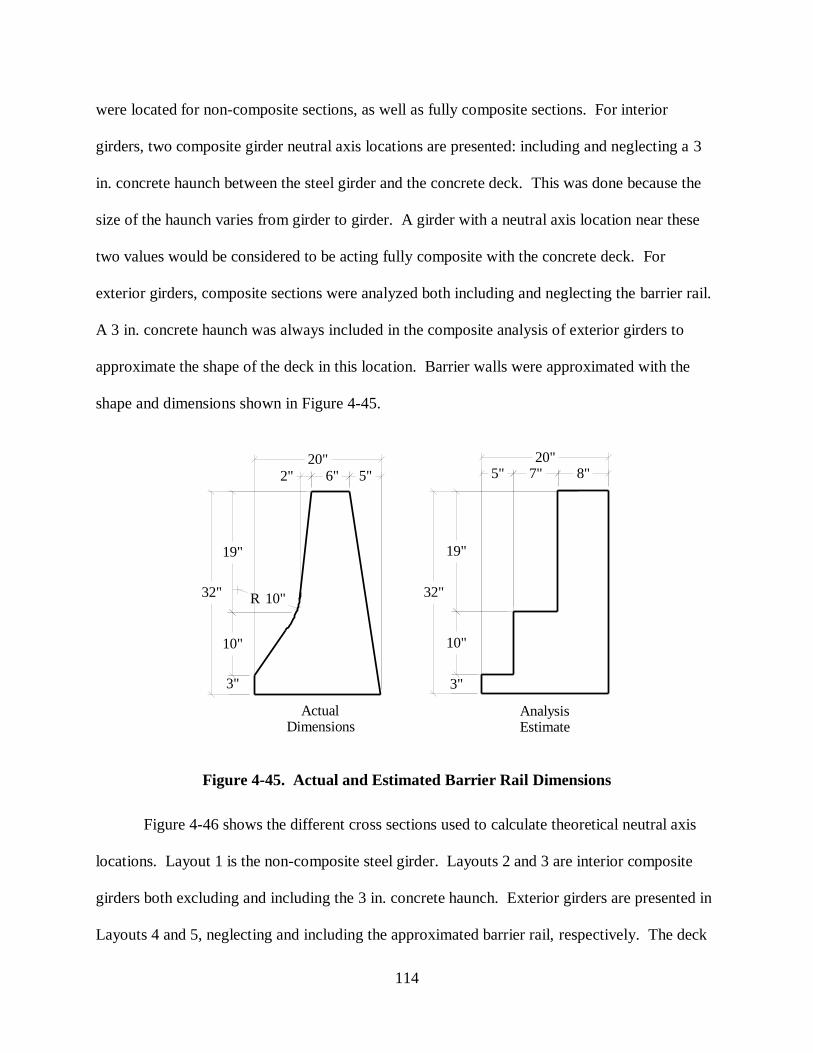
114

were located for non-composite sections, as well as fully composite sections. For interior

girders, two composite girder neutral axis locations are presented: including and neglecting a 3

in. concrete haunch between the steel girder and the concrete deck. This was done because the

size of the haunch varies from girder to girder. A girder with a neutral axis location near these

two values would be considered to be acting fully composite with the concrete deck. For

exterior girders, composite sections were analyzed both including and neglecting the barrier rail.

A 3 in. concrete haunch was always included in the composite analysis of exterior girders to

approximate the shape of the deck in this location. Barrier walls were approximated with the

shape and dimensions shown in Figure 4-45.

Figure 4-45. Actual and Estimated Barrier Rail Dimensions

Figure 4-46 shows the different cross sections used to calculate theoretical neutral axis

locations. Layout 1 is the non-composite steel girder. Layouts 2 and 3 are interior composite

girders both excluding and including the 3 in. concrete haunch. Exterior girders are presented in

Layouts 4 and 5, neglecting and including the approximated barrier rail, respectively. The deck

32"

19"

10"

3"

20"5" 7" 8"

AnalysisEstimate

6"2"

R 10"

3"

32"

20"5"

ActualDimensions

10"

19"

115

layout for an exterior girder is an approximation of the geometry present on the bridge. Table 4-

27 presents these theoretical values for comparison with experimental results. All values are

given in inches, and measured from the bottom of the steel girder.

Figure 4-46. Composite Girder Cross Sections Used for Neutral Axis Calculation

Table 4-27. Calculated Neutral Axis Locations

Location Girder Layout Neutral Axis Location, in.

Modulus of Elasticity (ksi) 3605 4220 4650 Average

Four

Tenths

of Span

Length

1 22.7 22.7 22.7 22.7

2 45.9 47.4 48.2 47.2

3 48.2 49.7 50.7 49.5

4 46.0 47.6 48.6 47.4

5 54.3 56.0 57.0 55.8

Center

Support

1 44.2 44.2 44.2 44.2

2 67.7 69.6 70.8 69.4

3 70.0 72.0 73.2 71.7

4 61.1 62.4 63.2 62.2

5 70.3 72.0 73.0 71.8

4.6.2 Neutral Axis Experimental Results at Four Tenths of Span Length

Peak experimental strain values recorded during pseudo-static testing were plotted using

spreadsheet software. The trend line function was then used to determine the neutral axis

1 2 543

116

location. Using a linear trend line, the y-intercept value represents the neutral axis of the

composite beam. North and South Span data are presented on each plot. Trend line equations

are located on each plot beside the legend designation with which they correspond. Because all

strain profile plots are very similar, only one load scenario for each girder is presented here. All

other plots can be found in Appendix J. Concrete strains recorded on the bottom of the deck

during North Span testing are significantly different than top flange strains. This is thought to be

due to shear lag between the deck and the girder. This difference in strain introduces error in the

determination of neutral axis locations. For this reason, North Span neutral axis locations have

been determined from only the top and bottom strain values.

Figure 4-47 presents the strain profile for Girder 1 under loading Scenario A. Analysis of

strains under this loading scenario produced neutral axis locations of 50.2 in. and 54.7 in. for the

North and South Spans, respectively.

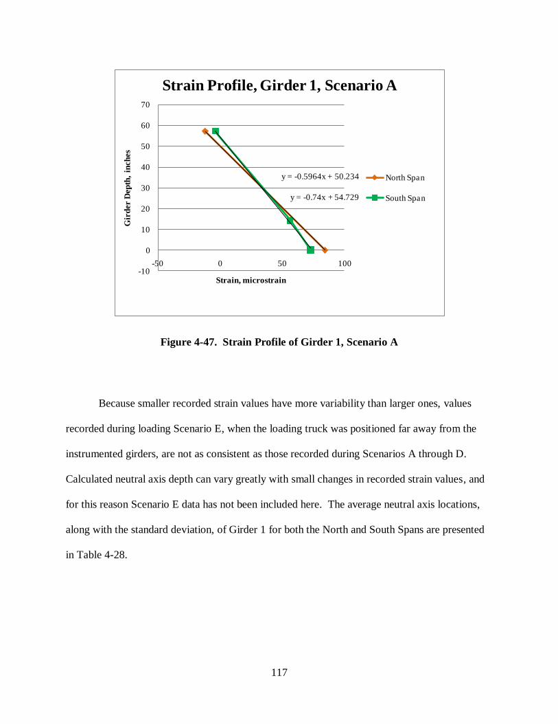
117

Figure 4-47. Strain Profile of Girder 1, Scenario A

Because smaller recorded strain values have more variability than larger ones, values

recorded during loading Scenario E, when the loading truck was positioned far away from the

instrumented girders, are not as consistent as those recorded during Scenarios A through D.

Calculated neutral axis depth can vary greatly with small changes in recorded strain values, and

for this reason Scenario E data has not been included here. The average neutral axis locations,

along with the standard deviation, of Girder 1 for both the North and South Spans are presented

in Table 4-28.

y = -0.5964x + 50.234

y = -0.74x + 54.729

-10

0

10

20

30

40

50

60

70

-50 0 50 100

Gir

der D

ep

th,

inch

es

Strain, microstrain

Strain Profile, Girder 1, Scenario A

North Span

South Span

118

Table 4-28. Average Neutral Axis Locations of Girder 1

Girder 1 North Span South Span

Average N.A.

Location,

inches

Standard

Deviation

53.3

0.65 1.01

49.8

Presented in Figure 4-48 is the strain profile data for Girder 2 recorded during loading

Scenario A. Analysis of strains on Girder 2 under this loading scenario produced neutral axis

locations of 44.4 in. and 45.1 in. for the North and South Spans, respectively.

Figure 4-48. Strain Profile of Girder 2, Scenario A

y = -0.7439x + 44.395

y = -0.7079x + 45.109

-10

0

10

20

30

40

50

60

70

-40 -20 0 20 40 60 80

Gir

der D

ep

th,

inch

es

Strain, microstrain

Strain Profile, Girder 2, Scenario A

North Span

South Span

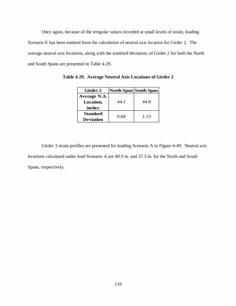
119

Once again, because of the irregular values recorded at small levels of strain, loading

Scenario E has been omitted from the calculation of neutral axis location for Girder 2. The

average neutral axis locations, along with the standard deviation, of Girder 2 for both the North

and South Spans are presented in Table 4-29.

Table 4-29. Average Neutral Axis Locations of Girder 2

Girder 2 North Span South Span

Average N.A.

Location,

inches

44.1 44.8

Standard

Deviation0.68 1.13

Girder 3 strain profiles are presented for loading Scenario A in Figure 4-49. Neutral axis

locations calculated under load Scenario A are 40.9 in. and 37.3 in. for the North and South

Spans, respectively.

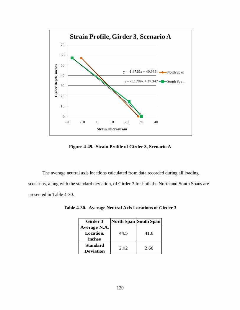
120

Figure 4-49. Strain Profile of Girder 3, Scenario A

The average neutral axis locations calculated from data recorded during all loading

scenarios, along with the standard deviation, of Girder 3 for both the North and South Spans are

presented in Table 4-30.

Table 4-30. Average Neutral Axis Locations of Girder 3

Girder 3 North Span South Span

Average N.A.

Location,

inches

44.5 41.8

Standard

Deviation2.02 2.68

y = -1.4729x + 40.936

y = -1.1789x + 37.347

0

10

20

30

40

50

60

70

-20 -10 0 10 20 30 40

Gir

der D

ep

th,

inch

es

Strain, microstrain

Strain Profile, Girder 3, Scenario A

North Span

South Span

121

4.6.3 Neutral Axis Comparison at Four Tenths of Span Length

The following plots compare experimental neutral axis locations with those calculated.

Presented are the results for Girders 1 through 3 for North and South Spans. For interior girders,

comparisons are presented with composite sections both including and excluding the 3 in.

concrete haunch between the girder and deck, and for exterior girders comparisons are made

with composite sections both including and ignoring the barrier rail. In all plots the location of

the non-composite neutral axis is presented for comparison purposes. As before, all values are

given in inches measured from the bottom of the steel girder.

Figure 4-50 presents the comparison for Girder 1. A fully composite girder and deck,

neglecting barrier rail, has a neutral axis 47.4 in. from the girder bottom. Including the barrier

rail increases the location to 55.8 in. Experimental results for Girder 1 from the North and South

Spans indicate neutral axis locations of about 50 in. and 53 in., respectively. Considering the

deviation in the recorded data, Girder 1 can be considered to be acting fully composite with the

deck and barrier rail on both the North and South Spans at this location of the bridge.

122

Figure 4-50. Girder 1 Neutral Axis Comparison

Figure 4-51 presents the neutral axis comparison for Girder 2. A fully composite girder

and deck, neglecting the 3 in. concrete haunch above the girder, has a neutral axis 47.2 in. from

the girder bottom. Including the haunch increases the location to 49.5 in. Experimental results

for Girder 2 indicate neutral axis locations of about 44 in. and 45 in., for the North and South

Spans, respectively. On each span, Girder 2 is behaving with between 80 per cent and 90 per

cent composite action, depending on the depth of the concrete haunch. No measurements of the

concrete haunches were made during testing. However, examining photographs taken during

testing, it appears that all concrete haunches are between 2 and 3 in. tall, indicating that the

amount of composite action occurring on the South Span of Girder 2 should be taken on the

lower end of the given range.

49.853.3

22.7

55.8

47.4

0

20

40

60

N.A

. Loca

tion

, in

ches

Girder 1 Neutral Axis Comparison

North Span Measured South Span Measured

Non-Composite Composite w/ Barrier Rail

Composite w/o Barrier Rail

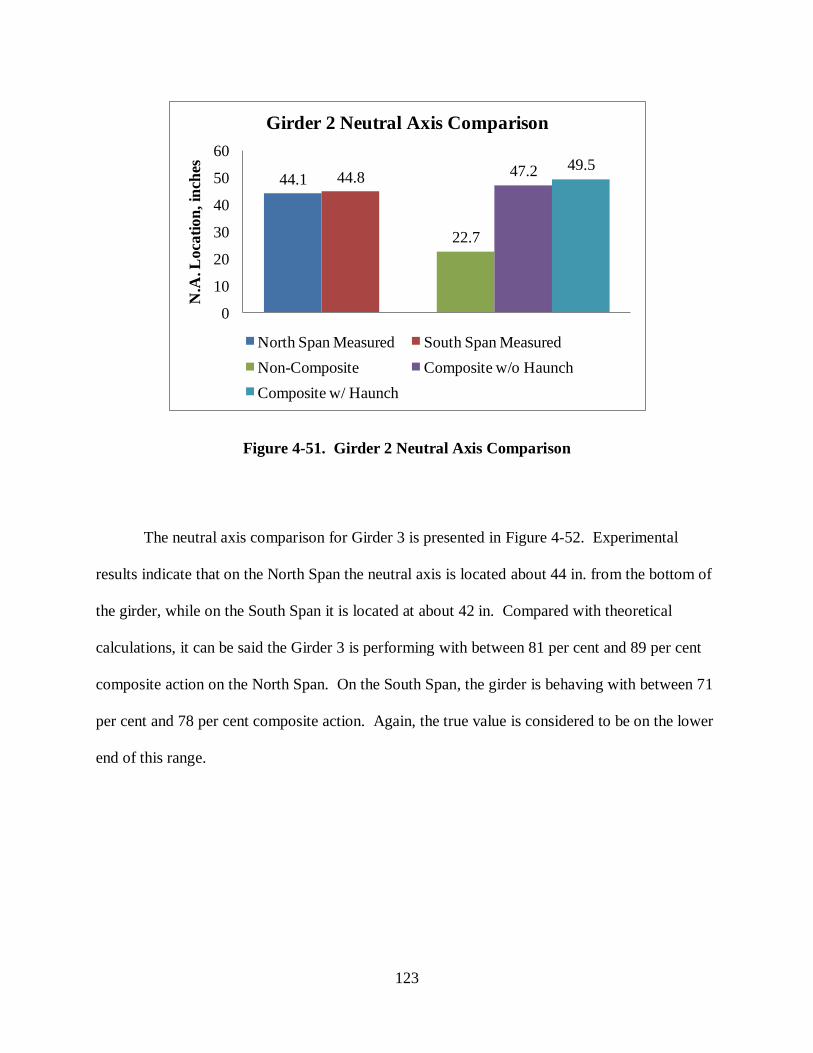
123

Figure 4-51. Girder 2 Neutral Axis Comparison

The neutral axis comparison for Girder 3 is presented in Figure 4-52. Experimental

results indicate that on the North Span the neutral axis is located about 44 in. from the bottom of

the girder, while on the South Span it is located at about 42 in. Compared with theoretical

calculations, it can be said the Girder 3 is performing with between 81 per cent and 89 per cent

composite action on the North Span. On the South Span, the girder is behaving with between 71

per cent and 78 per cent composite action. Again, the true value is considered to be on the lower

end of this range.

44.1 44.8

22.7

47.2 49.5

0

10

20

30

40

50

60

N.A

. Lo

cati

on

, in

ches

Girder 2 Neutral Axis Comparison

North Span Measured South Span Measured

Non-Composite Composite w/o Haunch

Composite w/ Haunch

124

Figure 4-52. Girder 3 Neutral Axis Comparison

4.6.4 Neutral Axis Comparison with NDE Results

Deck deterioration of the U.S. Route 15 bridge has been mapped out through the use of

ground penetrating radar (GPR) by Nenad Gucunski and his team at Rutgers University. Figure

4-53 compares a GPR image of the bridge with a plan view of the bridge identifying the

locations where possible loss of composite action were detected. Shown in red on the GPR

image, it can be seen that there is substantial deck deterioration on the South Span near Girders 2

and 3 at the location of instrumentation that indicated potential loss of composite action. In

comparison, the NDE data suggests that there is less deck deterioration on the North Span of the

bridge. This is consistent with the neutral axis analysis of Girder 3, which acts with greater

composite action on the North Span than on the South Span.

44.541.8

22.7

47.2 49.5

0

10

20

30

40

50

60

N.A

. Lo

cati

on

, in

ches

Girder 3 Neutral Axis Comparison

North Span Measured South Span Measured

Non-Composite Composite w/o Haunch

Composite w/ Haunch

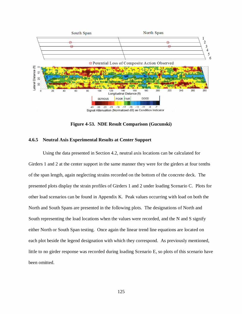
125

Figure 4-53. NDE Result Comparison (Gucunski)

4.6.5 Neutral Axis Experimental Results at Center Support

Using the data presented in Section 4.2, neutral axis locations can be calculated for

Girders 1 and 2 at the center support in the same manner they were for the girders at four tenths

of the span length, again neglecting strains recorded on the bottom of the concrete deck. The

presented plots display the strain profiles of Girders 1 and 2 under loading Scenario C. Plots for

other load scenarios can be found in Appendix K. Peak values occurring with load on both the

North and South Spans are presented in the following plots. The designations of North and

South representing the load locations when the values were recorded, and the N and S signify

either North or South Span testing. Once again the linear trend line equations are located on

each plot beside the legend designation with which they correspond. As previously mentioned,

little to no girder response was recorded during loading Scenario E, so plots of this scenario have

been omitted.

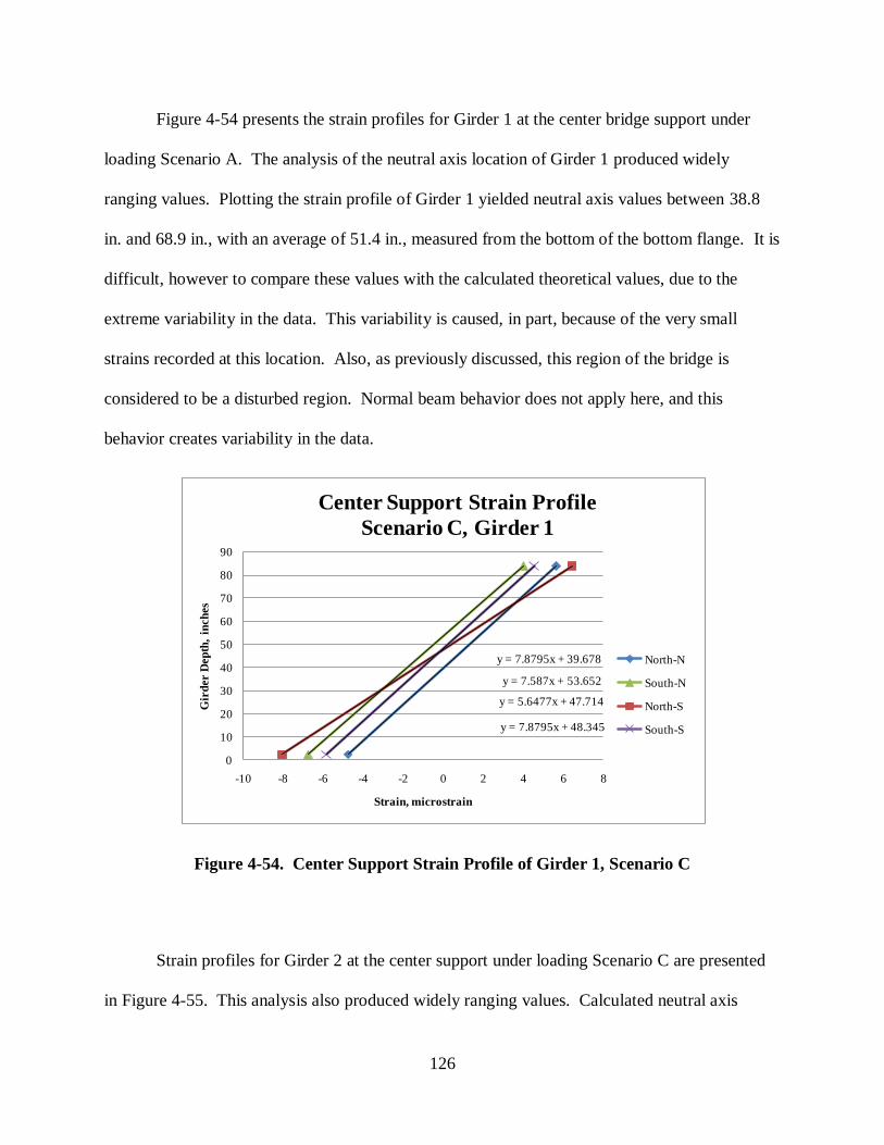
126

Figure 4-54 presents the strain profiles for Girder 1 at the center bridge support under

loading Scenario A. The analysis of the neutral axis location of Girder 1 produced widely

ranging values. Plotting the strain profile of Girder 1 yielded neutral axis values between 38.8

in. and 68.9 in., with an average of 51.4 in., measured from the bottom of the bottom flange. It is

difficult, however to compare these values with the calculated theoretical values, due to the

extreme variability in the data. This variability is caused, in part, because of the very small

strains recorded at this location. Also, as previously discussed, this region of the bridge is

considered to be a disturbed region. Normal beam behavior does not apply here, and this

behavior creates variability in the data.

Figure 4-54. Center Support Strain Profile of Girder 1, Scenario C

Strain profiles for Girder 2 at the center support under loading Scenario C are presented

in Figure 4-55. This analysis also produced widely ranging values. Calculated neutral axis

y = 7.8795x + 39.678

y = 7.587x + 53.652

y = 5.6477x + 47.714

y = 7.8795x + 48.345

0

10

20

30

40

50

60

70

80

90

-10 -8 -6 -4 -2 0 2 4 6 8

Gir

der D

ep

th,

inch

es

Strain, microstrain

Center Support Strain Profile

Scenario C, Girder 1

North-N

South-N

North-S

South-S

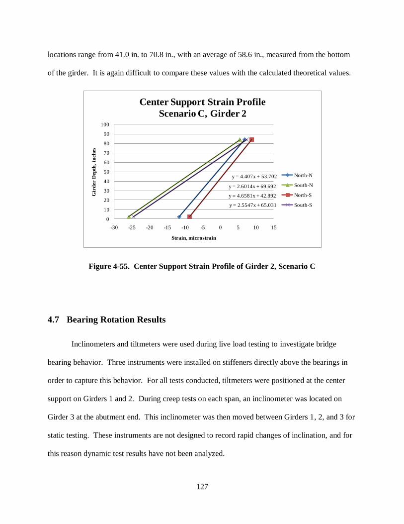
127

locations range from 41.0 in. to 70.8 in., with an average of 58.6 in., measured from the bottom

of the girder. It is again difficult to compare these values with the calculated theoretical values.

Figure 4-55. Center Support Strain Profile of Girder 2, Scenario C

4.7 Bearing Rotation Results

Inclinometers and tiltmeters were used during live load testing to investigate bridge

bearing behavior. Three instruments were installed on stiffeners directly above the bearings in

order to capture this behavior. For all tests conducted, tiltmeters were positioned at the center

support on Girders 1 and 2. During creep tests on each span, an inclinometer was located on

Girder 3 at the abutment end. This inclinometer was then moved between Girders 1, 2, and 3 for

static testing. These instruments are not designed to record rapid changes of inclination, and for

this reason dynamic test results have not been analyzed.

y = 4.407x + 53.702

y = 2.6014x + 69.692

y = 4.6581x + 42.892

y = 2.5547x + 65.031

0

10

20

30

40

50

60

70

80

90

100

-30 -25 -20 -15 -10 -5 0 5 10 15

Gir

der D

ep

th,

inch

es

Strain, microstrain

Center Support Strain Profile

Scenario C, Girder 2

North-N

South-N

North-S

South-S

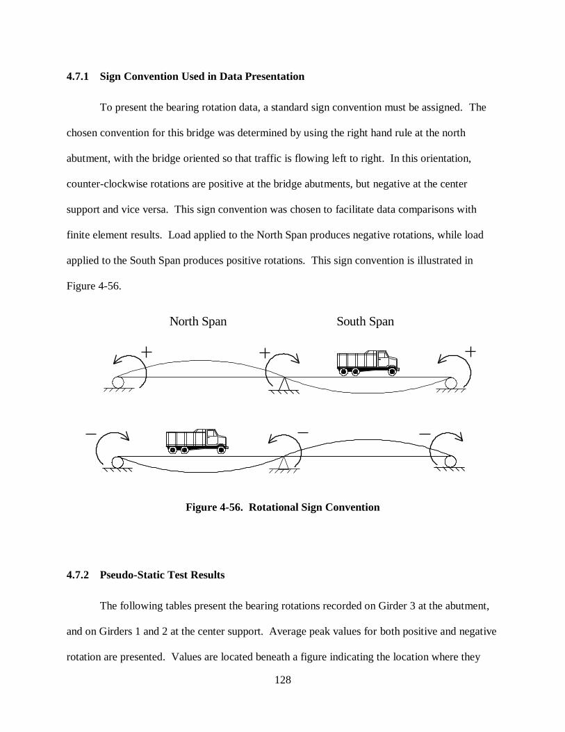
128

4.7.1 Sign Convention Used in Data Presentation

To present the bearing rotation data, a standard sign convention must be assigned. The

chosen convention for this bridge was determined by using the right hand rule at the north

abutment, with the bridge oriented so that traffic is flowing left to right. In this orientation,

counter-clockwise rotations are positive at the bridge abutments, but negative at the center

support and vice versa. This sign convention was chosen to facilitate data comparisons with

finite element results. Load applied to the North Span produces negative rotations, while load

applied to the South Span produces positive rotations. This sign convention is illustrated in

Figure 4-56.

Figure 4-56. Rotational Sign Convention

4.7.2 Pseudo-Static Test Results

The following tables present the bearing rotations recorded on Girder 3 at the abutment,

and on Girders 1 and 2 at the center support. Average peak values for both positive and negative

rotation are presented. Values are located beneath a figure indicating the location where they

North Span South Span

129

were recorded, either at the center support or the north or south abutments. Data tables including

the average and maximum recorded values, the standard deviation of the data, and number of

tests conducted can be found in Appendix L. Data from each span is presented together for

comparison purposes, and all values are in degrees x 10-4

. Because of the chosen sign

convention, positive rotations at the abutment end of one span should be compared with negative

rotations of the other span. Instrumentation recording rotations at the center support was located

in the exact same location for each span tested. For this reason, it was anticipated that data from

the North and South Spans would be close, if not identical. As will be seen, this was not the

case.

During testing many problems occurred with the titlmeters positioned at the center

support. Values recorded on each day were very similar from test to test, but testing from one

day to another (North Span versus South Span testing days), revealed extremely different results.

The tiltmeters also seemed to not work at all during some tests, recording only noise with no

discernable rotation behavior. This malfunction seemed to be random, and no explanation for it

is known. Compounding these issues are the extremely small rotations recorded at the center

support, which can increase data variability. Because of the inconsistencies with the tiltmeters,

results of center support bearing rotations are not of much value. Nonetheless, they are

presented as recorded for comparison with future test data.

Table 4-31 presents the bearing rotation data recorded during Scenario A testing.

Positive rotations recorded on Girder 3 at the north abutment should be compared with negative

values at the south abutment. For this load case, the rotations of both the north and south

abutments had similar magnitudes. Positive north abutment rotations can be compared to

negative south abutment rotations. This is identified in Table 4-31 with comparable values in

130

bold. Positive rotations recorded on Girder 1 at the center support were similar to one another,

although negative rotations were off by almost a factor of two. The titlmeter on Girder 2 did not

record quality data for either the North or South Span under this loading configuration.

Table 4-31. Bearing Rotations, Scenario A

Girder 3 Girder 1 6

68 Girder 2 N/A

Girder 1 5 Girder 3

Girder 2 N/A 224

Girder 3 Girder 1 -9

-181 Girder 2 N/A

Girder 1 -5 Girder 3

Girder 2 N/A -84

North Span

Testing

South Span

Testing

Positive

Rotations

South Span

Testing

Bearing Rotations (degrees x 10-4

), Scenario A

Negative

Rotations

North Span

Testing

North Span South Span

North Span South Span

Bearing rotation data for loading Scenario B is presented in Table 4-32. Rotations

recorded at the abutments were once again of similar magnitudes. Comparing center support

rotations of Girder 2 recorded on North and South Span testing, it can be seen that the results are

fairly similar. This cannot be said for Girder 1 results, where positive rotations were off from

one another by more than a factor of two.

131

Table 4-32. Bearing Rotations, Scenario B

Girder 3 Girder 1 7

138 Girder 2 6

Girder 1 3 Girder 3

Girder 2 8 478

Girder 3 Girder 1 -12

-433 Girder 2 -2

Girder 1 -9 Girder 3

Girder 2 -3 -159

North Span

Testing

South Span

Testing

South Span

Testing

Negative

Rotations

Bearing Rotations (degrees x 10-4

), Scenario B

Positive

Rotations

North Span

Testing

North Span South Span

North Span South Span

Results for bearing rotations recorded during loading Scenario C are shown in Table 4-

33. Abutment rotations at the north and south abutments, both positive and negative, are very

similar to one another. Girder 2 rotations at the center span seem to be fairly consistent from one

day to the next, but still not as consistent as they should be. No comparison can be made for

Girder 1 because the tiltmeter did not produce quality data in this scenario during testing of the

South Span.

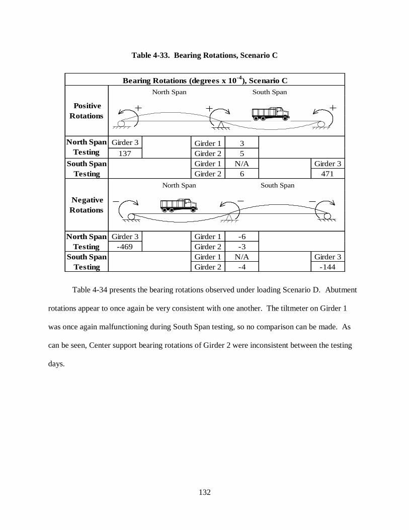
132

Table 4-33. Bearing Rotations, Scenario C

Girder 3 Girder 1 3

137 Girder 2 5

Girder 1 N/A Girder 3

Girder 2 6 471

Girder 3 Girder 1 -6

-469 Girder 2 -3

Girder 1 N/A Girder 3

Girder 2 -4 -144

North Span

Testing

South Span

Testing

South Span

Testing

Negative

Rotations

Bearing Rotations (degrees x 10-4

), Scenario C

Positive

Rotations

North Span

Testing

North Span South Span

North Span South Span

Table 4-34 presents the bearing rotations observed under loading Scenario D. Abutment

rotations appear to once again be very consistent with one another. The tiltmeter on Girder 1

was once again malfunctioning during South Span testing, so no comparison can be made. As

can be seen, Center support bearing rotations of Girder 2 were inconsistent between the testing

days.

133

Table 4-34. Bearing Rotations, Scenario D

Girder 3 Girder 1 1

70 Girder 2 2

Girder 1 N/A Girder 3

Girder 2 3 248

Girder 3 Girder 1 -4

-247 Girder 2 -1

Girder 1 N/A Girder 3

Girder 2 -2 -74

North Span

Testing

South Span

Testing

South Span

Testing

Negative

Rotations

Bearing Rotations (degrees x 10-4

), Scenario D

Positive

Rotations

North Span

Testing

North Span South Span

North Span South Span

Load Scenario E bearing rotations are presented in Table 4-35. Rotations recorded at

either abutment are once again of similar magnitudes. Positive rotations of Girder 1 at the center

support are fairly similar, but the negative rotations are off by almost a factor of two. For Girder

2, value comparisons between North and South Span testing are off significantly for both

positive and negative rotations.

134

Table 4-35. Bearing Rotations, Scenario E

Girder 3 Girder 1 3

64 Girder 2 2

Girder 1 3 Girder 3

Girder 2 3 168

Girder 3 Girder 1 -2

-181 Girder 2 -3

Girder 1 -4 Girder 3

Girder 2 -3 -56

North Span

Testing

South Span

Testing

South Span

Testing

Negative

Rotations

Bearing Rotations (degrees x 10-4

), Scenario E

Positive

Rotations

North Span

Testing

North Span South Span

North Span South Span

4.7.3 Static Test Results

Static tests were performed in an effort to capture bearing rotations to a higher degree of

resolution than was possible during pseudo-static testing. Loading trucks were arranged in the

same loading scenarios used for all other testing, but were stopped with their front tires at 0.25

and 0.65 times the span length. Bearing rotations were recorded on Girders 1 and 2 at the center

support, and on Girders 1, 2, and 3 at the abutments. Due to the amount of time these tests took

to set up, only a limited number were performed.

As previously mentioned, the tiltmeters located at the center support behaved erratically

throughout testing, and it seems that they were not working at times during static testing. It is

hard to determine the quality of the recorded data because of the limited number of tests

135

performed. Unfortunately, on test number 27 of South Span testing, the load truck was

accidentally positioned at two tenths of the span length.

Due to the limited number of tests performed, no statistical analysis was performed on

this data. Results of each static test performed are presented in Table 4-36.

Table 4-36. Static Testing Rotations

Instrument Location

1 2 3 1 2

0.25 - - -130 -2 N/A

0.65 - - -152 -8 N/A

0.25 -32 - - -3 N/A

0.65 -34 - - -8 N/A

0.25 - -417 - -3 N/A

0.65 - -421 - -12 N/A

0.25 - - -243 0 N/A

0.65 - - -202 -7 N/A

0.25 287 - - 1 2

0.65 318 - - 4 4

0.25 282 - - 2 2

0.65 322 - - 5 4

0.20 - 351 - N/A 2

0.65 - 470 - N/A 6

0.25 - 450 - 1 4

0.65 - 466 - 4 7

South

25 A

26 A

27 B

28 B

22 B

23 C

Girder NumberLoad Location

ScenarioTest #Span

Static Rotations (degrees x 10-4

)

Abutment Center Support

North

20 A

21 A

4.8 Expansion Joint Translation Results

As discussed in Chapter 3, expansion joint translations were measured through the use of

LVDTs located on the deck, set to span across the joint opening. These values are used for

comparison with results from finite element models to examine the stiffness effects expansion

136

joints may have on bridge performance. The values are also used to calculate rotation occurring

at girder ends, which are then compared with measured bearing rotation values.

4.8.1 Translation Results

Expansion joint movements were recorded at two different points during each test. While

North Span tests were occurring, both LVDTs were located on the expansion joint at the north

abutment. These two LVDTs were then moved to the south abutment expansion joint during

South Span testing. Each LVDT was located on the deck 6 in. from the barrier rail. LVDT 1

was located on the right side of the bridge when facing the direction of travel, near Girder 1, and

LVDT 2 was located on the left side of the bridge, close to Girder 6. Measurements were taken

as positive when the joints opened and negative as the joints closed. Presented in Table 4-37 and

Table 4-38 are the average and maximum peak values recorded during pseudo-static testing with

each LVDT, both positive and negative, in inches x 10-3

. Also included in the tables is the

standard deviation of the data and the number of tests performed. As previously discussed,

LVDT 1 was hit by the load truck on the first run of North Span testing, so no results are

available for this location.

137

Table 4-37. North Expansion Joint Movements

Scenario Open Close Open Close

8.8 -7.1 N/A N/A

9.9 -7.6 N/A N/A

1.43 0.41 N/A N/A

20.1 -15.8 N/A N/A

20.4 -16.8 N/A N/A

0.28 0.86 N/A N/A

23.5 -19.3 N/A N/A

24.0 -20.0 N/A N/A

0.38 0.53 N/A N/A

10.4 -9.3 N/A N/A

10.7 -9.7 N/A N/A

0.24 0.38 N/A N/A

16.8 -11.6 N/A N/A

18.0 -11.8 N/A N/A

0.75 0.19 N/A N/A

North Expansion Joint Movement (inches x 10-3

)

LVDT Loction (Number) Left (2) Right (1)

Average

Maximum

Standard Deviation

Average

Maximum

Standard DeviationA

B

Number of Tests 3 N/A

Number of Tests 4 N/A

Average

Maximum

Standard Deviation

Average

Maximum

Standard DeviationC

D

Number of Tests 4 N/A

Number of Tests 4 N/A

Average

Maximum

Standard DeviationE

Number of Tests 4 N/A

138

Table 4-38. South Expansion Joint Movement

Scenario Open Close Open Close

4.84 -4.95 22.62 -10.06

5.46 -5.46 23.06 -10.57

0.46 0.65 0.42 0.46

14.26 -12.47 37.00 -17.40

16.38 -13.57 39.03 -18.17

1.45 1.28 1.36 0.64

21.56 -13.36 28.41 -15.71

22.39 -13.36 29.43 -16.71

0.60 N/A 0.76 0.79

4 1

10.26 -7.03 13.96 -7.84

11.01 -7.46 14.60 -8.25

0.53 0.30 0.51 0.27

17.99 -10.34 8.72 -6.77

18.51 -10.86 8.87 -7.72

0.49 0.68 0.15 0.91

LVDT Location (Number) Left (2) Right (1)

Average

Maximum

Standard Deviation

South Expansion Joint Movement (inches x 10-3

)

A

Number of Tests 4 4

Average

Maximum

Standard Deviation

Average

Maximum

Standard DeviationB

C

Number of Tests 4 4

Number of Tests 4

Average

Maximum

Standard Deviation

Average

Maximum

Standard DeviationD

E

Number of Tests 4 4

Number of Tests 3 3

4.8.2 Base Rotations Calculated from LVDT Results

Using the assumption from beam theory that plane sections remain plane, joint movement

data can be used to calculate bearing rotations. Although this idealized assumption that the

girder end and deck rotate together as a rigid body is not perfect, it will be used for comparison

purposes. The bearings at the abutment ends of the bridge are rocker bearings composed of a pin

connected to the bottom flange of the girder, and a rocker surface that bears on the abutment. It

139

is unclear which of these points represents the true axis of rotation for the bearing, and in reality

both probably contribute to the flexibility of the structure. For the purposes of this analysis,

however, it has been assumed that one point acts as the point of rotation while the other remains

fixed. Each recorded joint movement has been used to calculate two different angles of rotation;

one rotating about the bearing pin, using an arm of 69.125 in., and the other rotating about the

rocker bottom, using an arm of 77.125 in. These two measurements can be seen in Figure 4-57,

where the depth of the girder has been reduced for the sake of clarity. Bearing rotations are also

presented using the average of these two values.

Figure 4-57. Girder Dimensions at Abutment

1.5"

8.625"

1"

54"

1"

3"

8"

69.125"

77.125"

1"

1"

LVDT

Not to Scale

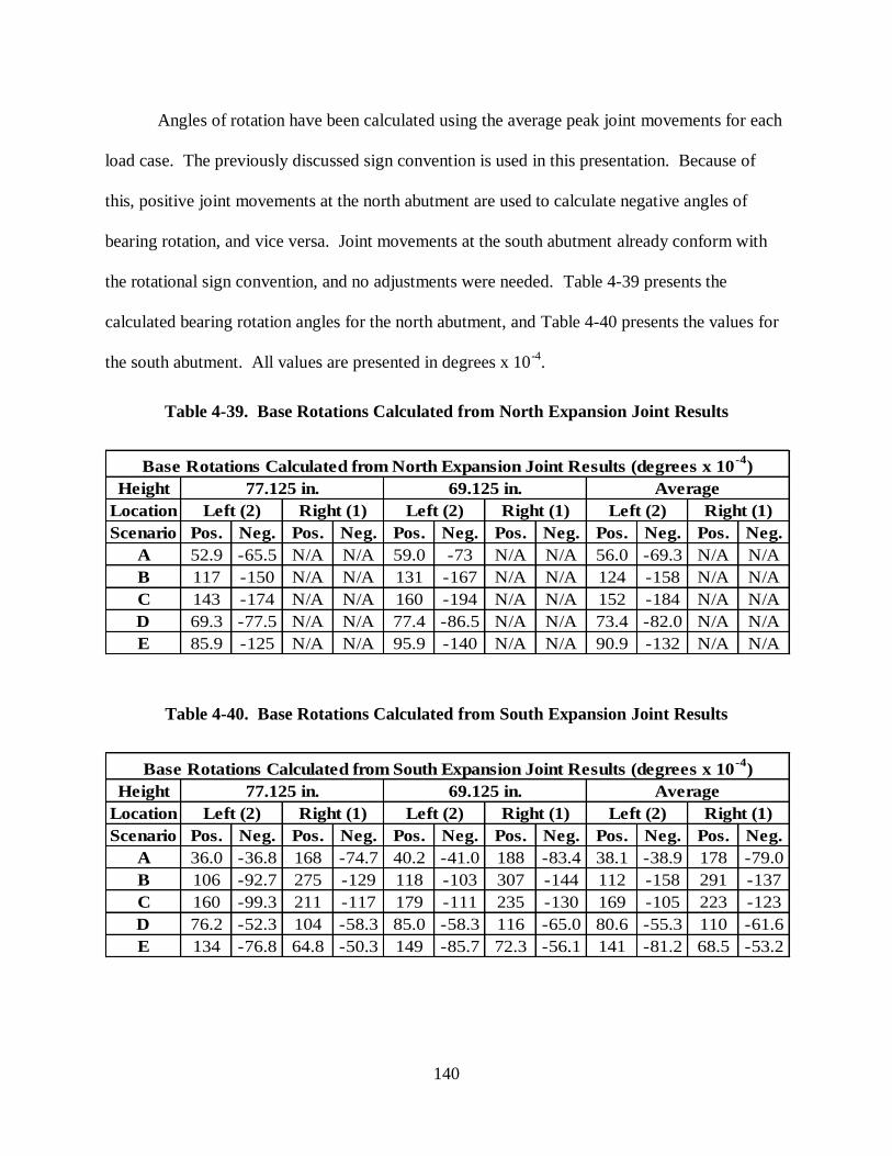
140

Angles of rotation have been calculated using the average peak joint movements for each

load case. The previously discussed sign convention is used in this presentation. Because of

this, positive joint movements at the north abutment are used to calculate negative angles of

bearing rotation, and vice versa. Joint movements at the south abutment already conform with

the rotational sign convention, and no adjustments were needed. Table 4-39 presents the

calculated bearing rotation angles for the north abutment, and Table 4-40 presents the values for

the south abutment. All values are presented in degrees x 10-4

.

Table 4-39. Base Rotations Calculated from North Expansion Joint Results

Height

Location

Scenario Pos. Neg. Pos. Neg. Pos. Neg. Pos. Neg. Pos. Neg. Pos. Neg.

A 52.9 -65.5 N/A N/A 59.0 -73 N/A N/A 56.0 -69.3 N/A N/A

B 117 -150 N/A N/A 131 -167 N/A N/A 124 -158 N/A N/A

C 143 -174 N/A N/A 160 -194 N/A N/A 152 -184 N/A N/A

D 69.3 -77.5 N/A N/A 77.4 -86.5 N/A N/A 73.4 -82.0 N/A N/A

E 85.9 -125 N/A N/A 95.9 -140 N/A N/A 90.9 -132 N/A N/A

69.125 in.

Left (2) Right (1)

77.125 in.

Base Rotations Calculated from North Expansion Joint Results (degrees x 10-4

)

Average

Left (2) Right (1)Left (2) Right (1)

Table 4-40. Base Rotations Calculated from South Expansion Joint Results

Height

Location

Scenario Pos. Neg. Pos. Neg. Pos. Neg. Pos. Neg. Pos. Neg. Pos. Neg.

A 36.0 -36.8 168 -74.7 40.2 -41.0 188 -83.4 38.1 -38.9 178 -79.0

B 106 -92.7 275 -129 118 -103 307 -144 112 -158 291 -137

C 160 -99.3 211 -117 179 -111 235 -130 169 -105 223 -123

D 76.2 -52.3 104 -58.3 85.0 -58.3 116 -65.0 80.6 -55.3 110 -61.6

E 134 -76.8 64.8 -50.3 149 -85.7 72.3 -56.1 141 -81.2 68.5 -53.2

77.125 in. 69.125 in. Average

Left (2) Right (1)

Base Rotations Calculated from South Expansion Joint Results (degrees x 10-4

)

Left (2) Right (1) Left (2) Right (1)

141

4.8.3 Comparison of LVDT Base Rotations with Recorded Bearing Rotations

Rotations calculated from expansion joint movements may be compared with bearing

rotations recorded at the abutments by inclinometers. Because only one girder was instrumented

with an inclinometer at the abutment and the LVDTs were located on the edges of the deck,

direct comparisons of rotation cannot be made. Overall rotational behavior at the abutment can

be observed however. Figure 4-58 presents the rotations occurring at the south abutment under

loading Scenario C for a typical test. Typical plots of rotation comparisons for all other loading

scenarios, as well as plots for the north abutment can be seen in Appendix M. To calculate

rotation angles from joint movements the average girder depth was used. LVDTs were located

on either side of the bridge, and designations of left and right indicate this in the following plots,

with left being located approximately above Girder 6, and right approximately above Girder 1.

The behavior exhibited in this figure shows rotations of Girder 3 were greater than those of

exterior Girders 1 and 6. This was expected for this loading condition, as the trucks were

loading Girder 3 maximally. More conclusions will be able to be drawn from this data in the

future after more live load tests are conducted.

142

Figure 4-58. Typical South Abutment Rotation Comparisons, Scenario C

4.9 Temperature Records

The temperature of Girders 1 and 2, as well as the surface temperature of the deck, were

recorded during testing. Girder temperatures, which were recorded through the use of

thermocouples, were averaged for each individual test, and then averaged for each testing

scenario. Deck temperatures were recorded at the beginning of each testing scenario with a

handheld thermometer. Thermocouple measurements are reported to the tenth of a degree, while

thermometer measurements are reported to the nearest degree. All temperatures listed in Table

4-41 are presented in degrees Fahrenheit.

0 100 2000.06

0.04

0.02

0

0.02

Right Side LVDT

Left Side LVDT

Inclinometer

South Abutment Girder 3 Bearing Rotation Comparison, Scenario C

Truck Position Along Bridge, feet

Rota

tion, deg

rees

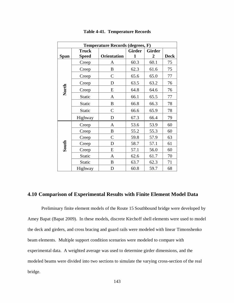
143

Table 4-41. Temperature Records

Temperature Records (degrees, F)

Span

Truck

Speed Orientation

Girder

1

Girder

2 Deck

Nort

h

Creep A 60.3 60.1 75

Creep B 62.3 61.6 75

Creep C 65.6 65.0 77

Creep D 63.5 63.2 76

Creep E 64.8 64.6 76

Static A 66.1 65.5 77

Static B 66.8 66.3 78

Static C 66.6 65.9 78

Highway D 67.3 66.4 79

Sou

th

Creep A 53.6 53.9 60

Creep B 55.2 55.3 60

Creep C 59.8 57.9 63

Creep D 58.7 57.1 61

Creep E 57.1 56.0 60

Static A 62.6 61.7 70

Static B 63.7 62.3 71

Highway D 60.8 59.7 68

4.10 Comparison of Experimental Results with Finite Element Model Data

Preliminary finite element models of the Route 15 Southbound bridge were developed by

Amey Bapat (Bapat 2009). In these models, discrete Kirchoff shell elements were used to model

the deck and girders, and cross bracing and guard rails were modeled with linear Timonshenko

beam elements. Multiple support condition scenarios were modeled to compare with

experimental data. A weighted average was used to determine girder dimensions, and the

modeled beams were divided into two sections to simulate the varying cross-section of the real

bridge.

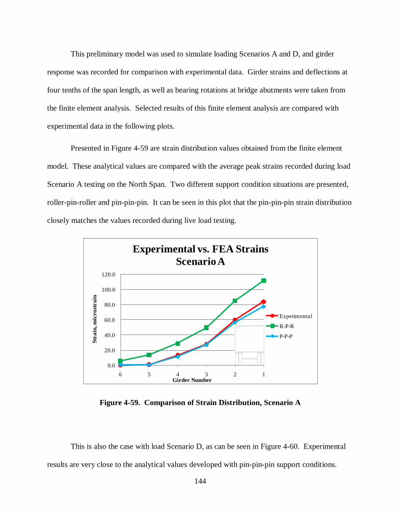
144

This preliminary model was used to simulate loading Scenarios A and D, and girder

response was recorded for comparison with experimental data. Girder strains and deflections at

four tenths of the span length, as well as bearing rotations at bridge abutments were taken from

the finite element analysis. Selected results of this finite element analysis are compared with

experimental data in the following plots.

Presented in Figure 4-59 are strain distribution values obtained from the finite element

model. These analytical values are compared with the average peak strains recorded during load

Scenario A testing on the North Span. Two different support condition situations are presented,

roller-pin-roller and pin-pin-pin. It can be seen in this plot that the pin-pin-pin strain distribution

closely matches the values recorded during live load testing.

Figure 4-59. Comparison of Strain Distribution, Scenario A

This is also the case with load Scenario D, as can be seen in Figure 4-60. Experimental

results are very close to the analytical values developed with pin-pin-pin support conditions.

0.0

20.0

40.0

60.0

80.0

100.0

120.0

123456

Str

ain

, m

icro

stra

in

Girder Number

Experimental vs. FEA Strains

Scenario A

Experimental

R-P-R

P-P-P

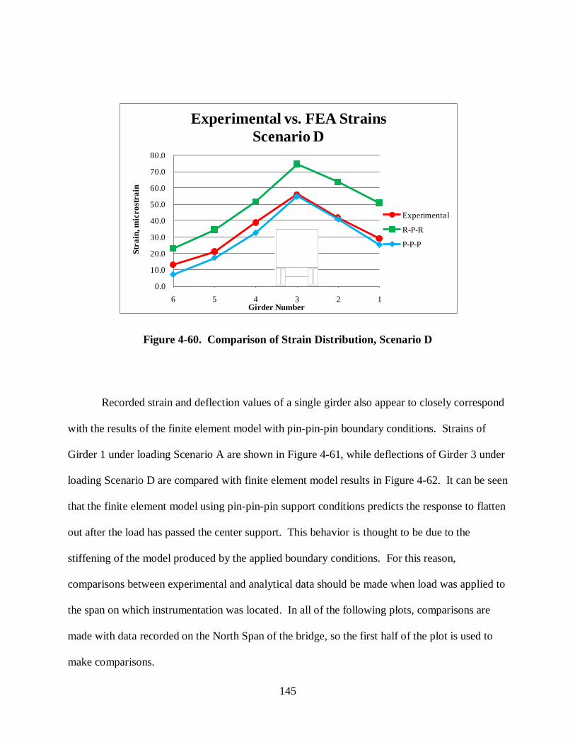
145

Figure 4-60. Comparison of Strain Distribution, Scenario D

Recorded strain and deflection values of a single girder also appear to closely correspond

with the results of the finite element model with pin-pin-pin boundary conditions. Strains of

Girder 1 under loading Scenario A are shown in Figure 4-61, while deflections of Girder 3 under

loading Scenario D are compared with finite element model results in Figure 4-62. It can be seen

that the finite element model using pin-pin-pin support conditions predicts the response to flatten

out after the load has passed the center support. This behavior is thought to be due to the

stiffening of the model produced by the applied boundary conditions. For this reason,

comparisons between experimental and analytical data should be made when load was applied to

the span on which instrumentation was located. In all of the following plots, comparisons are

made with data recorded on the North Span of the bridge, so the first half of the plot is used to

make comparisons.

0.0

10.0

20.0

30.0

40.0

50.0

60.0

70.0

80.0

123456

Str

ain

, m

icro

stra

in

Girder Number

Experimental vs. FEA Strains

Scenario D

Experimental

R-P-R

P-P-P

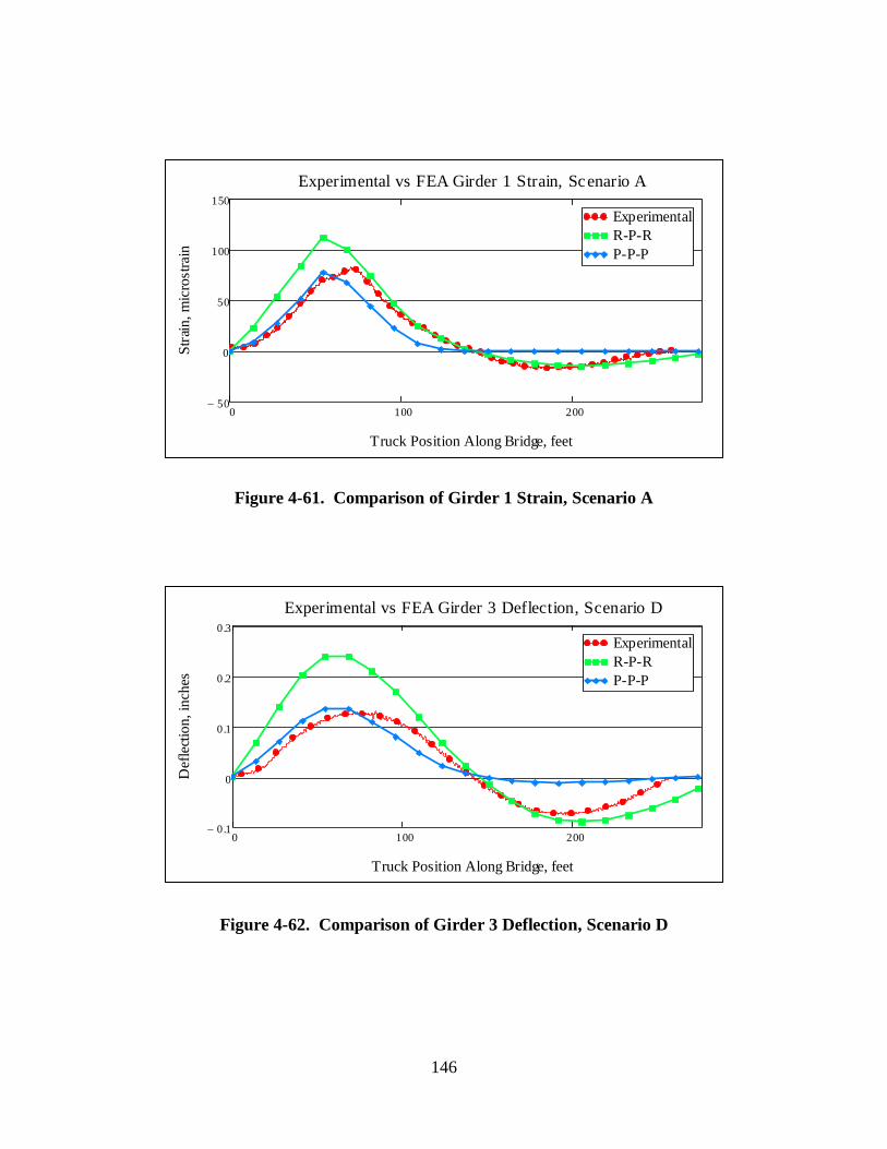
146

Figure 4-61. Comparison of Girder 1 Strain, Scenario A

Figure 4-62. Comparison of Girder 3 Deflection, Scenario D

0 100 20050

0

50

100

150

Experimental

R-P-R

P-P-P

Experimental vs FEA Girder 1 Strain, Scenario A

Truck Position Along Bridge, feet

Str

ain

, m

icro

stra

in

0 100 2000.1

0

0.1

0.2

0.3

Experimental

R-P-R

P-P-P

Experimental vs FEA Girder 3 Deflection, Scenario D

Truck Position Along Bridge, feet

Def

lect

ion

, in

ches

147

Experimental data corresponding to pin-pin-pin support condition values seems to

indicate that the bridge is behaving stiffer than would be expected. By looking only at this data,

it seems that changing support conditions are the source of behavioral changes. However, not all

response data compared similarly with finite element data from the pin-pin-pin model.

Bearing rotations at the bridge abutments do not indicate that the bridge is behaving with

pin-pin-pin support conditions. Experimentally recorded bearing rotations of Girder 3 under

loading Scenario A are compared with finite element results in Figure 4-63. This comparison

shows the experimental results bounded by the two different finite element models. Neither

roller-pin-roller nor pin-pin-pin accurately predicted the behavior observed during testing.

Figure 4-63. Comparison of Girder 3 Bearing Rotations, Scenario A

Bearing rotations of Girder 3 are again compared in Figure 4-64. The experimental data

presented was recorded during testing under load Scenario D. For this case, roller-pin-roller

finite element results closely predict the observed behavior.

0 100 2000.03

0.02

0.01

0

0.01

Experimental

R-P-R

P-P-P

Experimental vs FEA Abutment End Rotations of Girder 3, Scenario A

Truck Position Along Bridge, feet

Rota

tion, deg

rees

148

Figure 4-64. Comparison of Girder 3 Bearing Rotations, Scenario D

There are many reasons for the differences shown between predicted behavior and actual

bridge response. This finite element model was developed to represent the as-designed condition

of the bridge, and as such cannot be expected to represent the state of the bridge decades after

construction. Because of the observed deterioration of the bridge deck and other structural

components, it was never expected that the finite element model initially predict exact behavior.

Even though the model with pin-pin-pin support conditions accurately predicts both

strain and deflection response, it cannot be said that this model represents global bridge behavior.

There are a multitude of variables that influence bridge response, and some of these are not

accounted for in the finite element model. Unknown effects of skew, different structural

components, deterioration, and irregularity of materials all contribute to the variability of the

finite element analysis.

0 100 2000.03

0.02

0.01

0

0.01

Experimental

R-P-R

P-P-P

Experimental vs FEA Abutment End Rotations of Girder 3, Scenario D

Truck Position Along Bridge, feet

Ro

tatio

n, d

egre

es

149

Using the data obtained in this live load test, as well as that gathered during NDE and

material testing, refinements of the model will be made in an effort to better predict actual bridge

behavior.

150

Chapter 5: Conclusions and Recommendations

Multiple stiffness-related parameters were examined during live load testing of the U.S.

Route 15 southbound bridge. Comparisons of this data will be made with that from future live

load tests, yielding insight into the changing state of the bridge over time. As a result of this test,

the following conclusions and recommendations have been made.

5.1 Conclusions

Loading in the left and right travel lanes produces maximum response in Girders 5 and 3,

respectively.

Differences in behavior between strain and deflection response recorded at the same

location indicate changes in relative stiffness between bridge girders. This relative

stiffness difference is possibly due to the presence of barrier rails, stiffeners, and cross

bracing. Skew may also have an effect on changing relative stiffness between girders.

Local effects contributed to interesting strain values recorded on the bottom flange at the

center support. It is thought that this effect is due partially to the large bearing forces

present at this area of the bridge.

Distribution factors were calculated from experimental data to express the distribution of

load among girders. Comparisons between these factors and AASHTO design factors

show that in most cases AASHTO equations predict conservative load distribution. Only

one loading scenario out of five yielded distribution factors indicating that AASHTO

values are unconservative.

The load case for which AASHTO predicted unconservative moment distribution factors

was Scenario B, with two trucks attempting to maximally load Girder 5. When Girder 5,

151

the first interior girder, was maximally loaded, the AASHTO distribution factor was only

slightly unconservative compared with the experimental value. A distribution factor

calculated using the lever rule was shown to be conservative compared with the

experimental value. When this load scenario maximally loaded Girder 6, the exterior

girder, the AASHTO factor was very unconservative. For this case, the lever rule was

used to determine the load distribution factor. The girder spacing of the bridge does not

allow for the placement of two trucks outside of Girder 5 when applying the lever rule.

This is the cause for the unconservative distribution factor.

Skew of the bridge produced an increase in load distribution, resulting in a decrease in

distribution factor values. This decrease was between 3.8 per cent and eight per cent for

factors calculated using strain data, and 0.8 per cent to 2.2 per cent for factors calculated

using deflection.

Neutral axis locations appear to indicate that Girder 1 is acting fully composite with the

barrier rail at four tenths of the span length on both the North and South Spans.

Potential loss of composite action seen in some girders can be ascribed to loss of bond

between shear studs and concrete, delamination and other deterioration of the concrete

deck, and variability of material properties. This was observed on both spans of the

bridge in Girders 2 and 3. Girder 2 performed with between 80 per cent and 90 per cent

composite action on each span. Girder 3 was seen to have between 81 per cent and 89

per cent composite action on the North Span, and 71 per cent to 78 per cent composite

action on the South Span.

Bearing rotations recorded at the center support were inconsistent and the instruments

did not prove to be reliable. Data recorded at the abutments appear to be of good quality,

152

if limited in quantity. Indirect comparisons with joint movement data indicate that the

inclinometer recorded values of the proper magnitude.

Static testing did not yield statistically relevant data. The difficulty of the test along with

the amount of time required, make it difficult to justify this form of testing in future

research.

5.2 Recommendations

5.2.1 Recommendations for Long-Term Monitoring

Because Girders 3 and 5 produced the maximum strain response when load was

applied in the two traffic lanes, the majority of instrumentation during long-term

monitoring should be focused on these two girders.

Under the 50 kip truck load, the average maximum strain recorded on both girders

on both spans was around 55 microstrain. This value should be used as the trigger

value to begin data recording during long-term monitoring.

Long-term monitoring data should be recorded for 20 second intervals. This is

ample time to allow trucks to completely travel across the bridge. If trigger

values occur on the North Span, data should be recorded from five seconds before

the trigger occurred to fifteen seconds afterwards. If the South Span produces the

trigger, data should be recorded fifteen seconds prior to the trigger, and five

seconds after.

153

Strain gages located near the center support should be positioned far enough away

from the bearing to avoid the localized behavior.

Two LVDTs should be located at girder ends to capture both translation and

bearing rotation. The LVDTs should record with trigger values to capture load

related behavior, as well as periodically to capture temperature induced effects.

5.2.2 Recommendations for Future Live Load Testing

Pseudo-static testing is sufficient for all instrumentation, and pure static testing is

too time-consuming. Static testing should not be performed in the future.

When recording data to determine strain profiles, strain transducers located on the

web of the girder provide more consistent information than those located on the

bottom of the concrete deck. In future testing strain transducers should be located

on the web of the girder, one foot above the bottom flange.

Instrumentation should be arranged on the bridge following the skew of the

bridge, as well as perpendicular to the direction of travel. This may provide more

insight into the various effects skew has on bridge performance.

Deflectometers located at two tenths of the span length should be installed on all

six girders. Only positioning deflectometers on two girders created difficulty in

data analysis, and more instrumentation at this location would again yield more

insight into the effects of skew.

154

As discussed in the long-term monitoring recommendations, two LVDTs should

be located at girder ends to record girder translations and bearing rotations.

Two LVDTs should also be located on the abutment bearings to determine

whether the bearings are rotating about the rocker or the pin, or a combination of

the two.

Strain transducers should be installed on the bottom flange of girders right above

bearings at the abutment. This may allow for the observation of forces induced

by rotational resistance of deteriorated bearings.

More of the high quality inclinometers should be used to record bearing rotations.

Using only one inclinometer at the abutments greatly limited the ability to analyze

bearing rotations. Titlmeters used at the center support should be examined by

the manufacturer before being used in future testing. Although very high

resolution was shown, the accuracy and repeatability of these instruments seemed

to be extremely poor.

If possible, speeds greater than 25 miles per hour should be used for highway

speed tests. This should produce data capable of being used to calculate dynamic

load allowance.

5.2.3 Recommendations for Finite Element Model Refinement

Recommendations for the refinement of the finite element models are difficult to make at

this time. Although comparisons of strain and deflection data indicated that bearings were

behaving stiffer than would be expected, actual bearing rotation data recorded at the bridge

155

abutments contradicts this. Rotations observed at the center support are very small, possibly

indicating partial fixity at these bearings. This partial fixity could be introduced into the finite

element models through the use of rotational springs at these bearings.

Neutral axis analysis indicates that Girder 1 acts purely compositely with the barrier rail

on both the North and South Spans at four tenths of the span length. At the center support the

analysis was inconclusive, and no recommendations can be made at this location.

Girders 2 and 3 on the both spans appear to be acting with less than 100 per cent

composite action at four tenths of the span length. This may indicate shear stud loss or deck

delamination and deterioration, and this should be included in the finite element models.

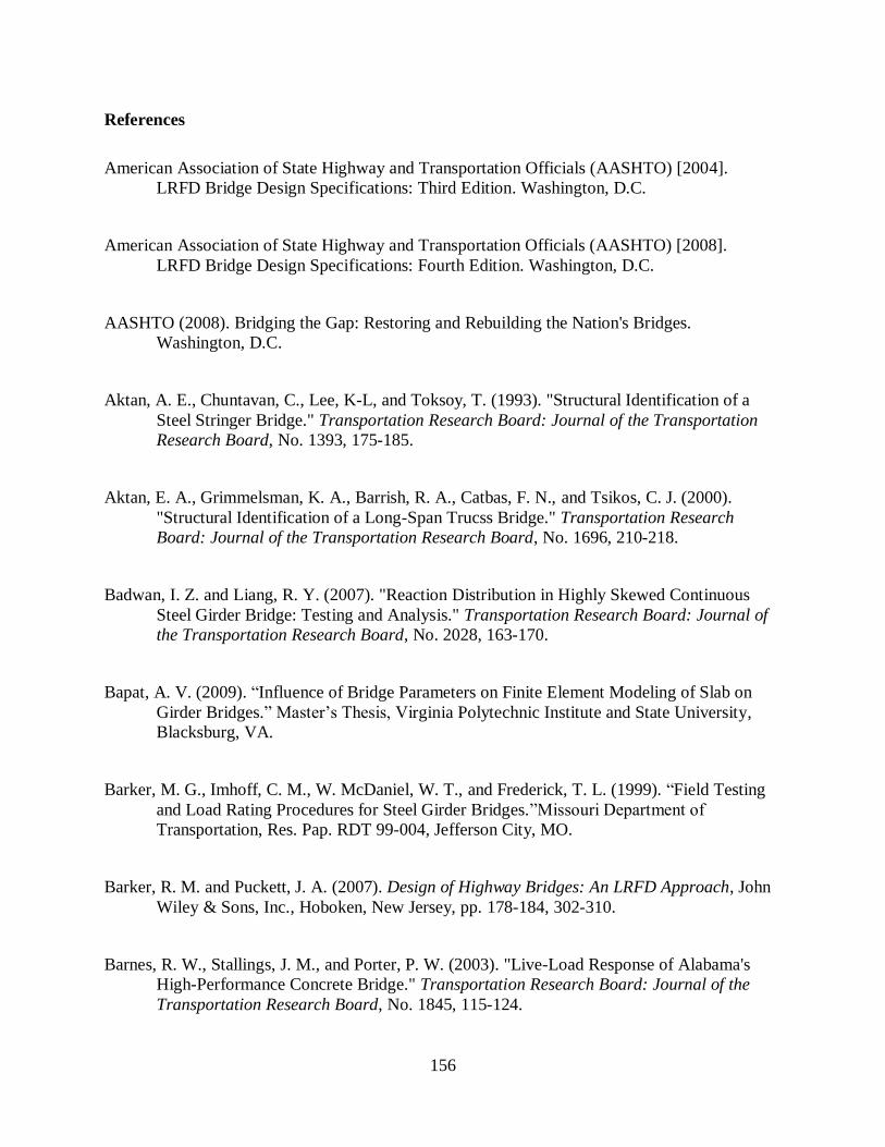
156

References

American Association of State Highway and Transportation Officials (AASHTO) [2004].

LRFD Bridge Design Specifications: Third Edition. Washington, D.C.

American Association of State Highway and Transportation Officials (AASHTO) [2008].

LRFD Bridge Design Specifications: Fourth Edition. Washington, D.C.

AASHTO (2008). Bridging the Gap: Restoring and Rebuilding the Nation's Bridges.

Washington, D.C.

Aktan, A. E., Chuntavan, C., Lee, K-L, and Toksoy, T. (1993). "Structural Identification of a

Steel Stringer Bridge." Transportation Research Board: Journal of the Transportation

Research Board, No. 1393, 175-185.

Aktan, E. A., Grimmelsman, K. A., Barrish, R. A., Catbas, F. N., and Tsikos, C. J. (2000).

"Structural Identification of a Long-Span Trucss Bridge." Transportation Research

Board: Journal of the Transportation Research Board, No. 1696, 210-218.

Badwan, I. Z. and Liang, R. Y. (2007). "Reaction Distribution in Highly Skewed Continuous

Steel Girder Bridge: Testing and Analysis." Transportation Research Board: Journal of

the Transportation Research Board, No. 2028, 163-170.

Bapat, A. V. (2009). “Influence of Bridge Parameters on Finite Element Modeling of Slab on

Girder Bridges.” Master’s Thesis, Virginia Polytechnic Institute and State University,

Blacksburg, VA.

Barker, M. G., Imhoff, C. M., W. McDaniel, W. T., and Frederick, T. L. (1999). “Field Testing

and Load Rating Procedures for Steel Girder Bridges.”Missouri Department of

Transportation, Res. Pap. RDT 99-004, Jefferson City, MO.

Barker, R. M. and Puckett, J. A. (2007). Design of Highway Bridges: An LRFD Approach, John

Wiley & Sons, Inc., Hoboken, New Jersey, pp. 178-184, 302-310.

Barnes, R. W., Stallings, J. M., and Porter, P. W. (2003). "Live-Load Response of Alabama's

High-Performance Concrete Bridge." Transportation Research Board: Journal of the

Transportation Research Board, No. 1845, 115-124.

157

Barr, P. J., Eberhard, M. O., and Stanton, J. F. (2001). "Live-Load Distribution Factors in

Prestressed Concrete Girder Bridges." Journal of Bridge Engineering, Vol. 6, No. 5, 298-

306.

Boresi, A. P. and Schmidt, R. J. (2003). Advanced Mechanics of Materials, John Wiley & Sons,

Inc., Hoboken, New Jersey, pp. 86-87

Chajes, M. J., Shenton, H. W., and O'Shea, D. (2000). "Bridge-condition Assessment and Load

Rating Using Nondestructive Evaluation Methods." Transportation Research Board:

Journal of the Transportation Research Board, Vol. 2, No. 1696, 83-91.

Chung, W., Liu., J., and Sotelino, E. (2006). "Influence of Secondary Elements and Deck

Cracking on the Lateral Load Distribution of Steel Girder Bridges." Journal of Bridge

Engineering, Vol. 11, No. 2, 178-187.

Clarke, S. N., Deatherage, J. H., Goodpasture, D., and Burdette, E. (1998). "Influence of Bridge

Approach, Surface Condition, and Velocity on Impact Factors for Fatigue-Prone Details."

Transportation Research Board: Journal of the Transportation Research Board, No.

1624, 166-179.

Cross, B., Vaughan, B., Panahshahi, N., Petermeier, D., Siow, Y., and Domagalski, T. (2009).

"Analytical and Experimental Investigation of Bridge Girder Shear Distribution Factors."

Journal of Bridge Engineering, Vol. 14, No. 3, 154-163.

Eom, J. and Nowak, A (2001). "Live Load Distribution for Steel Girder Bridges." Journal of

Bridge Engineering, Vol. 6, No. 6, 489-497.

Fu, C. C., Elhelbawey, M., Sahin, M. A., and Schelling, D. R. (1996). "Lateral Distribution

Factor from Bridge Field Testing." Journal of Structural Engineering, Vol. 122, No. 9,

1106-1109.

Gucunski, Nenad. Email. July 30, 2010.

Harris, D. K., Cousins, T., Murray, T. M., and Sotelino, E. D. (2008). "Field Investigation of a

Sandwich Plate System Bridge Deck." Journal of Performance of Constructed Facilities,

Vol. 22, No. 5, 305-315.

158

Hou, X., Yang, X., and Huang, Q. (2005). "Using Inclinometers to Measure Bridge Deflection."

Journal of Bridge Engineering, Vol. 10, No. 5, 564-569.

Hoult, N. A. (2010). "Long-Term Wireless Structural Health Monitoring of the Ferriby Road

Bridge." Journal of Bridge Engineering, Vol. 15, No. 2, 153-159.

Huang, H., Shenton, H. W., and Chajes, M. J. (2004). "Load Distribution for a Highly Skewed

Bridge: Testing and Analysis." Journal of Bridge Engineering, Vol. 9, No. 6, 558-562.

Huth, O. and Khbeis, H. (2007). "Pot Bearings Behavior After 32 Years of Service: In Situ and

Laboratory Tests." Engineering Structures, Vol. 29, No. 12, 3352-3363.

Kassner, B. L. (2004). “Long-Term In-Service Evaluation of Two Bridges Designed with Fiber-

Reinforced Polymer Girders.” Master’s Thesis, Virginia Polytechnic Institute and State

University, Blacksburg, VA.

Neely, W. D., Cousins, T. E., and Lesko, J. J. (2004). "Evaluation of In-Service Performance of

Tom's Creek Bridge Fiber-Reinforced Polymer Superstructure." Journal of Performance

of Constructed Facilities, Vol. 18, No. 3, 147-158.

Nowak, A. S., Eom, J., Sanli, A., and Till, R. (1999). "Verification of Girder Distribution Factors

for Short-Span Steel Girder Bridges by Field Testing." Transportation Research Board:

Journal of the Transportation Research Board, 62-67.

Park, K., Kim, S., Lee, Y., and Hwang, Y. (2005). "Degree of Composite Action Verification of

Bolted GFRP Bridge Deck-to-Girder Connection System." Composite Structures. Vol.

72, No. 3, 393-400.

Park, Y. S., Shin, D. K., and Chung, T. J. (2005). "Influence of Road Surface Roughness on

Dynamic Impact Factor of Bridge by Full-Scale Dynamic Testing." Canadian Journal of

Civil Engineering, Vol. 32, No. 5, 825-829.

Paultre, P., Chaallal, O., and Proulx, J. (1992). "Bridge Dynamics and Dynamic Amplification

Factors- A Review of Analytical and Experimental Findings." Canadian Journal of Civil

Engineering. Vol. 19, 260-278.

Pierce, P. C., Brungraber, R. L., Lichtenstein, A., Sabol, S., Morrell, J. J., and Lebow, S. T.

(2005). Covered Bridge Manual, Report No. FHWA-HRT-04-098, Washington, D.C.

159

Potisuk, T., and Higgins, C. (2007). "Field Testing and Analysis of CRC Deck Girder Bridges."

Journal of Bridge Engineering, Vol. 12, No. 1, 53-63.

Restrepo, E., Cousins, T., and Lesko, J. (2005). "Determination of Bridge Design Parameters

through Field Evaluation of the Route 601 Bridge Utilizing Fiber-Reinforced Polymer

Girders." Journal of Performance of Constructed Facilities, Vol. 19, No. 1, 17-27.

Roeder, C. W., Stanton, J. F., and Campbell, T. I. (1995). "Rotation of High Load Multirotational

Bridge Bearings." Journal of Structural Engineering, Vol. 121, No. 4, 747-756.

Saraf, V., Sokolik, A. F., and Nowak, A. S. (1996). "Proof Load Testing of Highway Bridges."

Transportation Research Board: Journal of the Transportation Research Board, No.

1541, 51-57.

Stallings, J. M. and Yoo, C. H. (1993). "Tests and Ratings of Short-Span Steel Bridges." Journal

of Structural Engineering, Vol. 119, No. 7, 2150-2168.

Stiller, W. B., Gergely, J., and Rochelle, R. (2006). "Testing, Analysis, and Evaluation of a

GFRP Deck on Steel Girders." Journal of Bridge Engineering, Vol. 11, No. 4, 394-400.

Weidner, J., Prader, J., Dubbs, N., Moon, F., and Aktan, E. (2009). “Structural Identification of

Bridges to Assess Safety and Performance.” Proceedings of the 2009 Structures

Congress, April 30 - May 2, 2009, Austin, TX, 119-124.

Yang, Y. and Meyers, J. J. (2003). "Live-Load Test Results of Missouri's First High-

Performance Concrete Superstructure Bridge." Transportation Research Board: Journal

of the Transportation Research Board, No. 1845, 96-103.

Zokaie, T., Imbsen, R. A., and Osterkamp, T. A. (1993). "Distribution of Wheel Loads on

Highway Bridges." Transportation Research Board: Journal of the Transportation

Research Board, No. 1290, 119-126.

160

APPENDIX A: CR Basic Program used with CR9000X

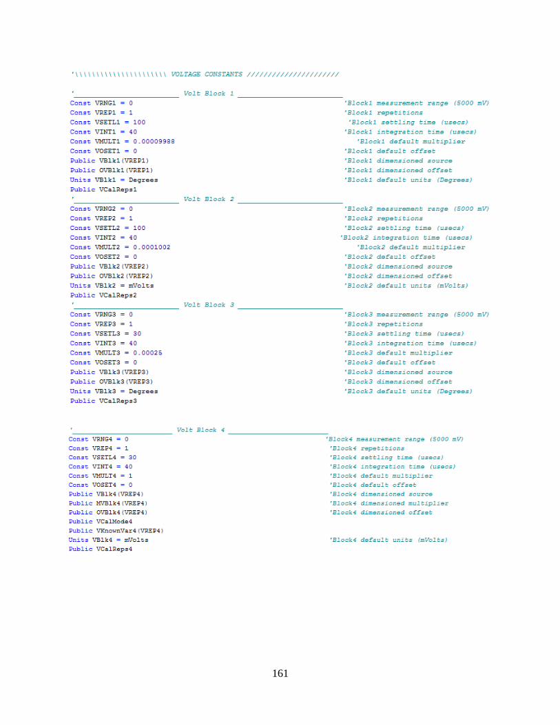
161

162

163

164

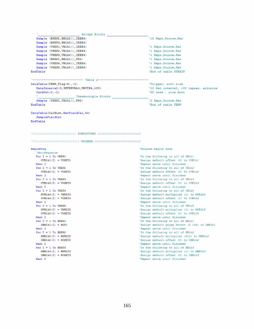
165

166

167

168

169

APPENDIX B: MathCad Data Analysis Routines

The filtering routine, seen below, takes a data set named “data” and completes a running

average for “n” points.

The zeroing routine, seen below, takes a data set named “data” and averages the first 100

points. All data in the set is then offset by this average value to zero the entire data set.

RunAvg data n( )

sum 0

sum sum datak

k j j n 1( )[ ]for

Dj

sum

n

j 1 rows data( ) n( )for

D

Zero data( )

sum 0

sum sum datak

k 1 100for

subsum

100

Dj

dataj

sub

j 1 rows data( )( )for

D

170

APPENDIX C: Live Load Test Data

Table C-1. North Span Service Strain Data

Test # Scenario 1 2 3 4 5 6 1 2 3 4 5 6

1 84.0 60.1 28.6 12.8 0.0 0.0 -19.6 -14.2 -10.8 -10.4 -5.0 0.0

2 84.3 58.8 28.0 12.9 1.9 0.0 -19.3 -12.6 -10.2 -8.9 -3.4 0.0

3 84.4 60.2 26.8 14.2 1.0 0.0 -19.9 -16.1 -12.1 -10.9 -5.0 0.0

4 109 106 86.1 49.0 25.8 13.5 -29.3 -22.7 -18.1 -14.9 -10.2 -8.7

5 112 107 84.6 46.8 22.0 10.8 -29.5 -23.1 -17.6 -15.4 -12.5 -11.6

6 109 105 84.6 45.4 20.6 11.9 -30.7 -24.1 -18.5 -15.8 -13.8 -8.8

7 110 106 82.8 45.2 19.8 10.9 -30.9 -25.4 -21.1 -15.9 -16.0 -10.7

16 56.6 80.8 96.3 78.4 44.8 28.5 -24.2 -19.8 -18.7 -15.7 -14.8 -18.2

17 58.9 82.2 93.7 76.3 45.1 30.3 -23.7 -20.5 -19.1 -16.1 -14.2 -18.5

18 57.3 81.6 94.7 76.4 43.0 30.9 -24.9 -21.3 -18.2 -15.6 -15.2 -16.0

19 58.4 81.4 96.4 73.9 41.8 30.5 -24.0 -20.2 -18.7 -15.8 -15.8 -14.5

8 30.0 42.9 55.3 39.6 21.0 13.2 -12.8 -10.4 -10.1 -7.8 -9.6 -10.0

9 28.6 41.3 54.9 38.6 21.0 12.3 -15.0 -14.0 -11.2 -11.7 -11.2 -8.1

10 28.6 41.3 54.9 38.6 21.0 12.3 -13.9 -12.0 -11.5 -9.7 -8.5 -11.2

11 28.8 42.1 57.4 38.9 20.6 12.5 -15.6 -13.3 -11.5 -9.6 -8.8 -9.9

12 8.7 15.8 26.9 48.3 55.4 41.7 -8.3 -9.1 -9.2 -11.6 -10.1 -17.6

13 9.3 16.5 26.9 49.4 54.6 41.5 -10.3 -11.1 -10.8 -12.1 -12.7 -15.1

14 9.3 16.5 26.9 49.4 54.6 41.5 -9.0 -9.9 -10.4 -11.7 -11.7 -18.0

15 10.1 16.9 29.4 51.4 55.2 42.8 -9.3 -9.2 -10.4 -10.5 -11.7 -15.4

Strains (με) Compression

A

B

C

North Span Service Strain Data

Strains (με) Tension

D

E

171

Table C-2. South Span Service Strain Data

Test # Scenario 1 2 3 4 5 6 1 2 3 4 5 6

1 74.3 60.7 30.9 15.1 3.0 0.0 -17.1 -13.6 -11.6 -9.4 -3.1 0.0

2 71.1 61.8 30.3 15.1 3.0 0.0 -15.2 -12.6 -11.9 -10.4 -4.0 0.0

3 71.8 61.7 29.3 16.1 4.0 0.0 -17.4 -14.4 -12.4 -9.8 -3.0 0.0

4 73.5 60.8 29.3 14.6 3.0 0.0 -18.6 -14.5 -12.2 -10.5 -3.0 0.0

5 91.4 104 86.4 50.3 24.6 9.0 -25.0 -20.3 -18.3 -15.4 -12.8 -10.0

6 92.7 106 85.3 50.0 25.6 9.0 -26.7 -22.0 -17.9 -16.1 -12.0 -9.0

7 92.8 107 84.9 49.4 23.8 8.0 -25.0 -21.0 -18.1 -16.3 -11.6 -9.0

8 88.9 103 83.4 50.5 22.6 9.0 -26.8 -22.3 -16.6 -14.6 -12.4 -8.0

17 48.7 78.3 90.8 80.8 46.9 28.6 -20.2 -19.0 -16.4 -17.6 -16.4 -16.8

18 49.2 75.6 90.5 81.3 47.4 28.5 -18.5 -18.4 -17.3 -14.9 -16.1 -18.4

19 48.2 75.0 91.2 82.0 46.0 27.6 -20.2 -20.2 -18.6 -16.5 -17.7 -17.4

20 47.3 74.7 90.5 82.2 47.1 28.3 -20.5 -19.1 -18.1 -16.2 -17.9 -17.7

13 24.7 39.1 54.6 38.9 20.2 15.0 -12.9 -11.3 -9.9 -9.8 -10.8 -9.9

14 24.5 38.3 55.3 40.4 22.5 15.1 -12.8 -11.3 -8.6 -9.7 -10.8 -9.5

15 25.7 39.3 55.5 41.0 22.2 13.6 -13.1 -10.9 -9.4 -9.5 -10.0 -11.3

16 25.9 38.4 54.2 40.6 22.1 14.7 -12.5 -12.8 -10.8 -9.8 -9.5 -10.2

9 8.7 16.5 27.6 52.3 57.5 45.0 -3.0 -6.8 -7.7 -8.8 -11.2 -13.8

10 7.6 13.7 25.9 50.2 56.0 41.9 -7.4 -7.1 -8.9 -11.6 -12.7 -17.8

11 6.9 12.9 24.4 48.5 53.5 43.1 -4.0 -8.7 -10.6 -12.0 -14.3 -16.3

12 8.9 13.9 27.2 52.0 57.1 41.4 -3.0 -7.6 -7.1 -10.6 -11.7 -17.3

South Span Service Strain Data

Strains (με) Tension Strains (με) Compression

D

E

A

B

C

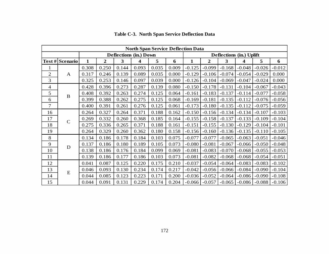
172

Table C-3. North Span Service Deflection Data

Test # Scenario 1 2 3 4 5 6 1 2 3 4 5 6

1 0.308 0.250 0.144 0.093 0.035 0.009 -0.125 -0.099 -0.168 -0.048 -0.026 -0.012

2 0.317 0.246 0.139 0.089 0.035 0.000 -0.129 -0.106 -0.074 -0.054 -0.029 0.000

3 0.325 0.253 0.146 0.097 0.039 0.000 -0.126 -0.104 -0.069 -0.047 -0.024 0.000

4 0.428 0.396 0.273 0.287 0.139 0.080 -0.150 -0.178 -0.131 -0.104 -0.067 -0.043

5 0.408 0.392 0.263 0.274 0.125 0.064 -0.161 -0.183 -0.137 -0.114 -0.077 -0.058

6 0.399 0.388 0.262 0.275 0.125 0.068 -0.169 -0.181 -0.135 -0.112 -0.076 -0.056

7 0.400 0.391 0.261 0.276 0.125 0.061 -0.173 -0.180 -0.135 -0.112 -0.075 -0.059

16 0.264 0.327 0.264 0.371 0.188 0.162 -0.150 -0.156 -0.134 -0.134 -0.107 -0.103

17 0.269 0.332 0.260 0.368 0.185 0.164 -0.155 -0.158 -0.137 -0.133 -0.109 -0.104

18 0.275 0.336 0.265 0.371 0.188 0.161 -0.151 -0.155 -0.130 -0.129 -0.104 -0.101

19 0.264 0.329 0.260 0.362 0.180 0.158 -0.156 -0.160 -0.136 -0.135 -0.110 -0.105

8 0.134 0.186 0.178 0.184 0.103 0.075 -0.077 -0.077 -0.065 -0.063 -0.051 -0.046

9 0.137 0.186 0.180 0.189 0.105 0.073 -0.080 -0.081 -0.067 -0.066 -0.050 -0.048

10 0.138 0.186 0.176 0.184 0.099 0.069 -0.081 -0.083 -0.070 -0.068 -0.055 -0.053

11 0.139 0.186 0.177 0.186 0.103 0.073 -0.081 -0.082 -0.068 -0.068 -0.054 -0.051

12 0.041 0.087 0.125 0.220 0.175 0.210 -0.037 -0.054 -0.064 -0.083 -0.083 -0.102

13 0.046 0.093 0.130 0.234 0.174 0.217 -0.042 -0.056 -0.066 -0.084 -0.090 -0.104

14 0.044 0.085 0.123 0.223 0.171 0.200 -0.036 -0.052 -0.064 -0.086 -0.090 -0.108

15 0.044 0.091 0.131 0.229 0.174 0.204 -0.066 -0.057 -0.065 -0.086 -0.088 -0.106

North Span Service Deflection Data

D

E

Deflections (in.) Down Deflections (in.) Uplift

A

B

C

173

Table C-4. South Span Service Deflection Data

Test # Scenario 1 2 3 4 5 6 1 2 3 4 5 6

1 0.317 0.254 0.181 0.104 0.040 0.000 -0.131 -0.109 -0.090 -0.063 -0.035 0.000

2 0.316 0.250 0.178 0.102 0.039 0.000 -0.126 -0.106 -0.084 -0.059 -0.030 0.000

3 0.317 0.248 0.174 0.097 0.037 0.000 -0.135 -0.115 -0.094 -0.069 -0.020 0.000

4 0.331 0.256 0.181 0.105 0.030 0.000 -0.139 -0.115 -0.091 -0.064 -0.020 0.000

5 0.421 0.379 0.389 0.267 0.135 0.078 -0.198 -0.183 -0.162 -0.125 -0.077 -0.064

6 0.433 0.387 0.397 0.266 0.131 0.060 -0.199 -0.185 -0.165 -0.129 -0.083 -0.050

7 0.428 0.383 0.388 0.261 0.129 0.060 -0.191 -0.179 -0.161 -0.123 -0.077 -0.060

8 0.424 0.381 0.390 0.267 0.134 0.076 -0.195 -0.183 -0.165 -0.126 -0.079 -0.065

17 0.279 0.325 0.400 N/A 0.209 0.169 -0.150 -0.159 -0.152 -0.138 -0.108 -0.113

18 0.279 0.324 0.397 N/A 0.208 0.168 -0.148 -0.150 -0.153 -0.134 -0.107 -0.112

19 0.275 0.321 0.395 N/A 0.206 0.170 -0.158 -0.157 -0.157 -0.138 -0.109 -0.111

20 0.275 0.322 0.397 N/A 0.206 0.171 -0.149 -0.149 -0.152 -0.137 -0.109 -0.114

13 0.148 0.188 0.226 0.189 0.104 0.077 -0.086 -0.084 -0.083 -0.075 -0.055 -0.058

14 0.148 0.187 0.226 0.191 0.107 0.081 -0.090 -0.088 -0.087 -0.077 -0.056 -0.056

15 0.148 0.188 0.226 0.190 0.106 0.081 -0.085 -0.082 -0.082 -0.074 -0.054 -0.056

16 0.152 0.192 0.233 0.199 0.111 0.084 -0.083 -0.082 -0.081 -0.072 -0.054 -0.057

9 0.048 0.092 0.156 0.227 0.206 0.238 -0.038 -0.045 -0.058 -0.067 -0.068 -0.093

10 0.040 0.084 0.147 0.213 0.190 0.214 -0.042 -0.053 -0.068 -0.084 -0.089 -0.118

11 0.042 0.084 0.147 0.213 0.188 0.218 -0.059 -0.066 -0.077 -0.090 -0.091 -0.119

12 0.046 0.087 0.147 0.212 0.189 0.216 -0.042 -0.053 -0.070 -0.085 -0.086 -0.113

D

E

South Span Service Deflection Data

A

B

C

Deflections (in.) Down Deflections (in.) Uplift

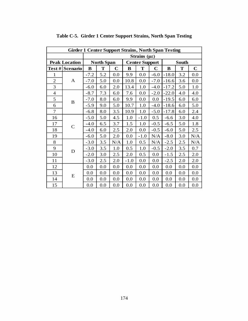
174

Table C-5. Girder 1 Center Support Strains, North Span Testing

Test # Scenario B T C B T C B T C

1 -7.2 5.2 0.0 9.9 0.0 -6.0 -18.0 3.2 0.0

2 -7.0 5.0 0.0 10.8 0.0 -7.0 -16.6 3.6 0.0

3 -6.0 6.0 2.0 13.4 1.0 -4.0 -17.2 5.0 1.0

4 -8.7 7.3 6.0 7.6 0.0 -2.0 -22.0 4.0 4.0

5 -7.0 8.0 6.0 9.9 0.0 0.0 -19.5 6.0 6.0

6 -5.9 9.0 5.0 10.7 1.0 -4.0 -18.6 6.0 5.0

7 -6.8 8.0 3.5 10.9 1.0 -5.0 -17.8 6.0 2.4

16 -5.0 5.0 4.5 1.0 -1.0 0.5 -6.6 3.0 4.0

17 -4.0 6.5 3.7 1.5 1.0 -0.5 -6.5 5.0 1.8

18 -4.0 6.0 2.5 2.0 0.0 -0.5 -6.0 5.0 2.5

19 -6.0 5.0 2.0 0.0 -1.0 N/A -8.0 3.0 N/A

8 -3.0 3.5 N/A 1.0 0.5 N/A -2.5 2.5 N/A

9 -3.0 3.5 1.0 0.5 1.0 -0.5 -2.0 3.5 0.7

10 -2.0 3.0 2.5 2.0 0.5 0.0 -1.5 2.5 2.0

11 -3.0 2.5 2.0 -1.0 0.0 0.0 -2.5 2.0 2.0

12 0.0 0.0 0.0 0.0 0.0 0.0 0.0 0.0 0.0

13 0.0 0.0 0.0 0.0 0.0 0.0 0.0 0.0 0.0

14 0.0 0.0 0.0 0.0 0.0 0.0 0.0 0.0 0.0

15 0.0 0.0 0.0 0.0 0.0 0.0 0.0 0.0 0.0

B

C

D

E

Girder 1 Center Support Strains, North Span Testing

Strains (με)

Peak Location

A

North Span Center Support South

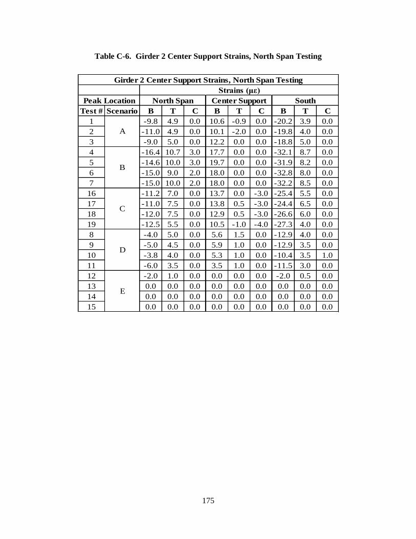
175

Table C-6. Girder 2 Center Support Strains, North Span Testing

Test # Scenario B T C B T C B T C

1 -9.8 4.9 0.0 10.6 -0.9 0.0 -20.2 3.9 0.0

2 -11.0 4.9 0.0 10.1 -2.0 0.0 -19.8 4.0 0.0

3 -9.0 5.0 0.0 12.2 0.0 0.0 -18.8 5.0 0.0

4 -16.4 10.7 3.0 17.7 0.0 0.0 -32.1 8.7 0.0

5 -14.6 10.0 3.0 19.7 0.0 0.0 -31.9 8.2 0.0

6 -15.0 9.0 2.0 18.0 0.0 0.0 -32.8 8.0 0.0

7 -15.0 10.0 2.0 18.0 0.0 0.0 -32.2 8.5 0.0

16 -11.2 7.0 0.0 13.7 0.0 -3.0 -25.4 5.5 0.0

17 -11.0 7.5 0.0 13.8 0.5 -3.0 -24.4 6.5 0.0

18 -12.0 7.5 0.0 12.9 0.5 -3.0 -26.6 6.0 0.0

19 -12.5 5.5 0.0 10.5 -1.0 -4.0 -27.3 4.0 0.0

8 -4.0 5.0 0.0 5.6 1.5 0.0 -12.9 4.0 0.0

9 -5.0 4.5 0.0 5.9 1.0 0.0 -12.9 3.5 0.0

10 -3.8 4.0 0.0 5.3 1.0 0.0 -10.4 3.5 1.0

11 -6.0 3.5 0.0 3.5 1.0 0.0 -11.5 3.0 0.0

12 -2.0 1.0 0.0 0.0 0.0 0.0 -2.0 0.5 0.0

13 0.0 0.0 0.0 0.0 0.0 0.0 0.0 0.0 0.0

14 0.0 0.0 0.0 0.0 0.0 0.0 0.0 0.0 0.0

15 0.0 0.0 0.0 0.0 0.0 0.0 0.0 0.0 0.0

C

D

E

Girder 2 Center Support Strains, North Span Testing

Strains (με)

Peak Location North Span Center Support South

A

B

176

Table C-7. Girder 1 Center Support Strains, South Span Testing

Test # Scenario B T C B T C B T C

1 -10.0 5.0 2.4 11.4 -2.0 -3.7 -13.6 3.6 2.8

2 -7.5 5.0 3.0 12.8 -1.5 -1.5 -12.6 3.5 3.4

3 -8.9 5.0 2.7 12.2 -1.0 -2.0 -14.5 3.2 2.8

4 -8.9 4.3 2.0 10.9 -1.5 -3.0 -15.8 2.5 2.6

5 -11.0 9.0 4.7 11.1 -1.0 -3.0 -16.3 7.0 4.0

6 -9.7 7.9 5.0 11.8 0.0 -2.0 -17.8 6.0 4.0

7 -10.0 8.5 4.2 11.0 0.0 -2.0 -15.7 6.2 4.0

8 -10.0 8.0 5.0 12.6 0.0 -2.0 -16.0 6.0 4.0

17 -8.0 6.5 5.0 1.0 0.0 0.0 -6.0 4.0 3.0

18 -8.6 6.7 4.5 1.0 1.0 0.0 -6.3 4.8 2.5

19 -7.9 6.0 4.3 1.0 0.5 0.0 -5.4 4.8 2.3

20 -7.7 6.5 5.2 2.0 0.0 0.0 -5.7 4.5 3.2

13 -4.0 3.5 3.0 1.0 0.0 0.0 -2.0 2.3 2.0

14 -5.0 3.5 3.2 0.0 0.0 1.0 -3.0 2.2 2.8

15 -4.3 3.0 2.5 0.5 0.0 0.5 -2.5 2.3 2.2

16 -4.5 2.5 2.3 0.0 -0.5 0.0 -2.6 1.0 0.7

9 0.0 0.0 0.0 0.0 0.0 0.0 0.0 0.0 0.0

10 0.0 1.0 0.0 0.0 0.0 0.0 0.0 0.5 0.0

11 0.0 0.0 0.0 0.0 0.0 0.0 0.0 0.0 0.0

12 0.0 0.0 0.0 0.0 0.0 0.0 0.0 0.0 0.0

Center Support South

Girder 1 Center Support Strains, South Span Testing

Strains (με)

Peak Location North Span

E

A

B

C

D

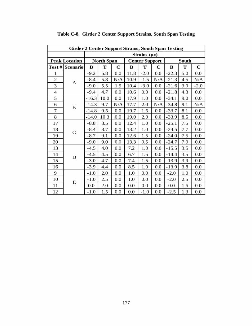
177

Table C-8. Girder 2 Center Support Strains, South Span Testing

Test # Scenario B T C B T C B T C

1 -9.2 5.8 0.0 11.8 -2.0 0.0 -22.3 5.0 0.0

2 -8.4 5.8 N/A 10.9 -1.5 N/A -21.3 4.5 N/A

3 -9.0 5.5 1.5 10.4 -3.0 0.0 -21.6 3.0 -2.0

4 -9.4 4.7 0.0 10.6 0.0 0.0 -21.8 4.3 0.0

5 -16.3 10.0 0.0 17.9 1.0 0.0 -34.1 9.0 0.0

6 -14.3 9.7 N/A 17.7 2.0 N/A -34.8 9.1 N/A

7 -14.8 9.5 0.0 19.7 1.5 0.0 -33.7 8.1 0.0

8 -14.0 10.3 0.0 19.0 2.0 0.0 -33.9 8.5 0.0

17 -8.8 8.5 0.0 12.4 1.0 0.0 -25.1 7.5 0.0

18 -8.4 8.7 0.0 13.2 1.0 0.0 -24.5 7.7 0.0

19 -8.7 9.1 0.0 12.6 1.5 0.0 -24.0 7.5 0.0

20 -9.0 9.0 0.0 13.3 0.5 0.0 -24.7 7.0 0.0

13 -4.5 4.0 0.0 7.2 1.0 0.0 -15.5 3.5 0.0

14 -4.5 4.5 0.0 6.7 1.5 0.0 -14.4 3.5 0.0

15 -3.0 4.7 0.0 7.4 1.5 0.0 -13.9 3.9 0.0

16 -3.9 4.4 0.0 8.5 1.0 0.0 -13.9 3.8 0.0

9 -1.0 2.0 0.0 1.0 0.0 0.0 -2.0 1.0 0.0

10 -1.0 2.5 0.0 1.0 0.0 0.0 -2.0 2.5 0.0

11 0.0 2.0 0.0 0.0 0.0 0.0 0.0 1.5 0.0

12 -1.0 1.5 0.0 0.0 -1.0 0.0 -2.5 1.3 0.0

Center Support South

Girder 2 Center Support Strains, South Span Testing

Strains (με)

Peak Location North Span

B

C

D

E

A

178

Table C-9. Deflections at Two Tenths of North Span

1 2 1 2

Test # Scenario

1 0.223 0.128 -0.070 -0.046

2 0.220 0.125 -0.075 -0.050

3 0.222 0.128 -0.076 -0.049

4 0.305 0.194 -0.123 -0.084

5 0.311 0.190 -0.122 -0.086

6 0.305 0.189 -0.122 -0.086

7 0.311 0.189 -0.119 -0.085

16 0.189 0.164 -0.097 -0.076

17 0.194 0.161 -0.098 -0.077

18 0.200 0.166 -0.096 -0.074

19 0.194 0.164 -0.100 -0.077

8 0.098 0.100 -0.048 -0.037

9 0.098 0.101 -0.051 -0.039

10 0.098 0.100 -0.050 -0.039

11 0.097 0.100 -0.051 -0.040

12 0.024 0.049 -0.022 -0.029

13 0.028 0.053 -0.022 -0.030

14 0.026 0.050 -0.020 -0.029

15 0.026 0.053 -0.023 -0.029

North Span Deflections at Two Tenths of Span

Girder #

Def. (in.) Down Def. (in.) Uplift

A

B

C

D

E

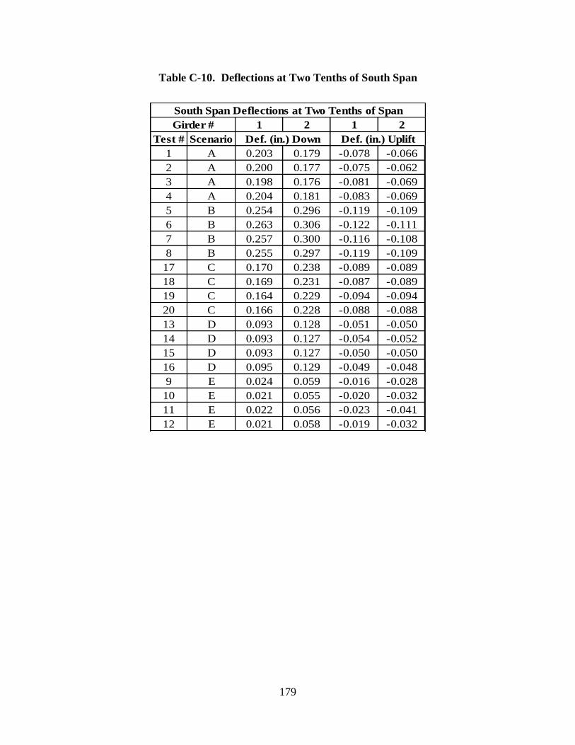
179

Table C-10. Deflections at Two Tenths of South Span

1 2 1 2

Test # Scenario

1 A 0.203 0.179 -0.078 -0.066

2 A 0.200 0.177 -0.075 -0.062

3 A 0.198 0.176 -0.081 -0.069

4 A 0.204 0.181 -0.083 -0.069

5 B 0.254 0.296 -0.119 -0.109

6 B 0.263 0.306 -0.122 -0.111

7 B 0.257 0.300 -0.116 -0.108

8 B 0.255 0.297 -0.119 -0.109

17 C 0.170 0.238 -0.089 -0.089

18 C 0.169 0.231 -0.087 -0.089

19 C 0.164 0.229 -0.094 -0.094

20 C 0.166 0.228 -0.088 -0.088

13 D 0.093 0.128 -0.051 -0.050

14 D 0.093 0.127 -0.054 -0.052

15 D 0.093 0.127 -0.050 -0.050

16 D 0.095 0.129 -0.049 -0.048

9 E 0.024 0.059 -0.016 -0.028

10 E 0.021 0.055 -0.020 -0.032

11 E 0.022 0.056 -0.023 -0.041

12 E 0.021 0.058 -0.019 -0.032

Girder #

Def. (in.) Down Def. (in.) Uplift

South Span Deflections at Two Tenths of Span

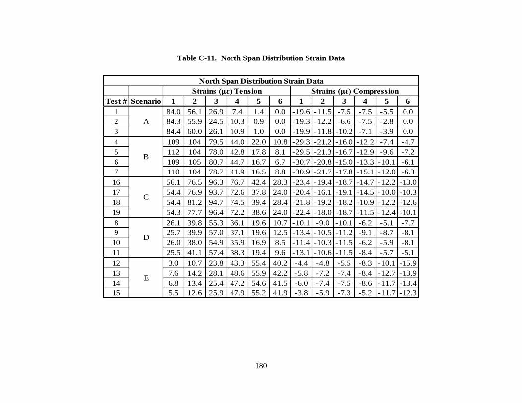
180

Table C-11. North Span Distribution Strain Data

Test # Scenario 1 2 3 4 5 6 1 2 3 4 5 6

1 84.0 56.1 26.9 7.4 1.4 0.0 -19.6 -11.5 -7.5 -7.5 -5.5 0.0

2 84.3 55.9 24.5 10.3 0.9 0.0 -19.3 -12.2 -6.6 -7.5 -2.8 0.0

3 84.4 60.0 26.1 10.9 1.0 0.0 -19.9 -11.8 -10.2 -7.1 -3.9 0.0

4 109 104 79.5 44.0 22.0 10.8 -29.3 -21.2 -16.0 -12.2 -7.4 -4.7

5 112 104 78.0 42.8 17.8 8.1 -29.5 -21.3 -16.7 -12.9 -9.6 -7.2

6 109 105 80.7 44.7 16.7 6.7 -30.7 -20.8 -15.0 -13.3 -10.1 -6.1

7 110 104 78.7 41.9 16.5 8.8 -30.9 -21.7 -17.8 -15.1 -12.0 -6.3

16 56.1 76.5 96.3 76.7 42.4 28.3 -23.4 -19.4 -18.7 -14.7 -12.2 -13.0

17 54.4 76.9 93.7 72.6 37.8 24.0 -20.4 -16.1 -19.1 -14.5 -10.0 -10.3

18 54.4 81.2 94.7 74.5 39.4 28.4 -21.8 -19.2 -18.2 -10.9 -12.2 -12.6

19 54.3 77.7 96.4 72.2 38.6 24.0 -22.4 -18.0 -18.7 -11.5 -12.4 -10.1

8 26.1 39.8 55.3 36.1 19.6 10.7 -10.1 -9.0 -10.1 -6.2 -5.1 -7.7

9 25.7 39.9 57.0 37.1 19.6 12.5 -13.4 -10.5 -11.2 -9.1 -8.7 -8.1

10 26.0 38.0 54.9 35.9 16.9 8.5 -11.4 -10.3 -11.5 -6.2 -5.9 -8.1

11 25.5 41.1 57.4 38.3 19.4 9.6 -13.1 -10.6 -11.5 -8.4 -5.7 -5.1

12 3.0 10.7 23.8 43.3 55.4 40.2 -4.4 -4.8 -5.5 -8.3 -10.1 -15.9

13 7.6 14.2 28.1 48.6 55.9 42.2 -5.8 -7.2 -7.4 -8.4 -12.7 -13.9

14 6.8 13.4 25.4 47.2 54.6 41.5 -6.0 -7.4 -7.5 -8.6 -11.7 -13.4

15 5.5 12.6 25.9 47.9 55.2 41.9 -3.8 -5.9 -7.3 -5.2 -11.7 -12.3

North Span Distribution Strain Data

Strains (με) Tension Strains (με) Compression

A

B

C

D

E

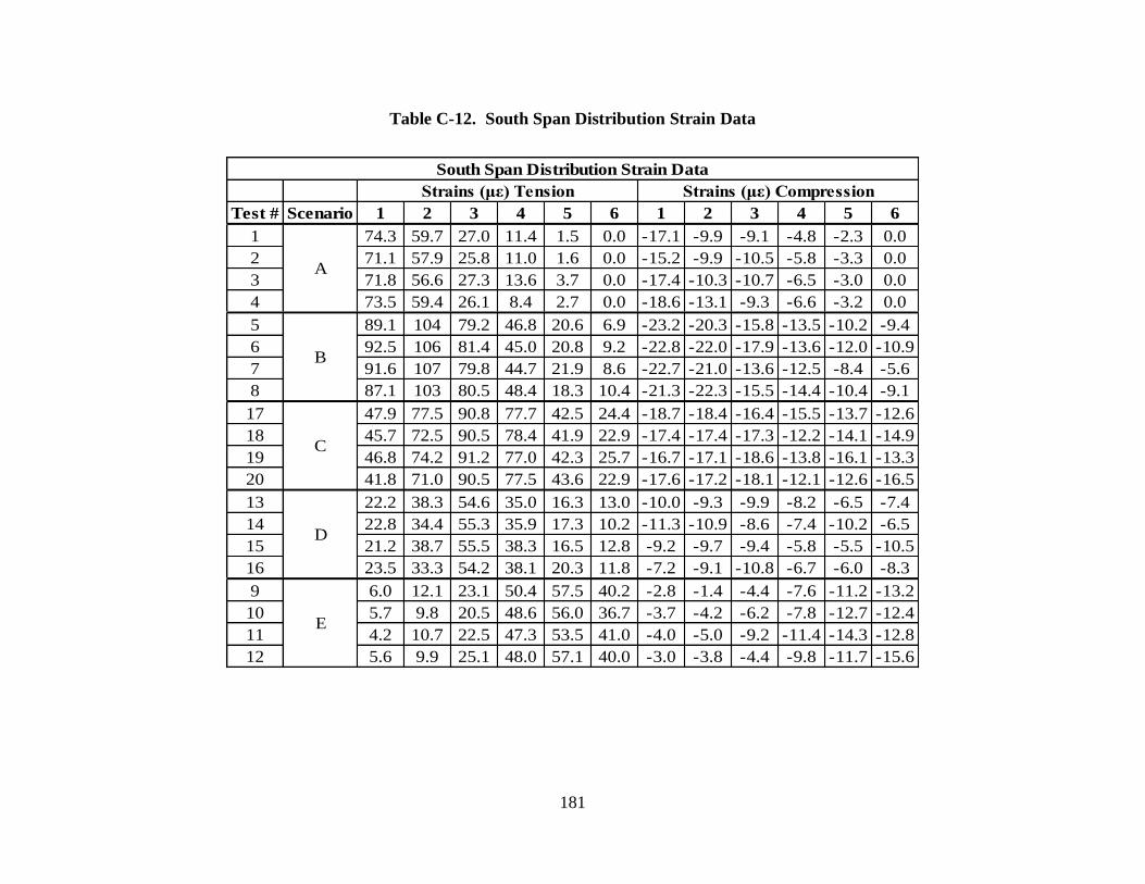
181

Table C-12. South Span Distribution Strain Data

Test # Scenario 1 2 3 4 5 6 1 2 3 4 5 6

1 74.3 59.7 27.0 11.4 1.5 0.0 -17.1 -9.9 -9.1 -4.8 -2.3 0.0

2 71.1 57.9 25.8 11.0 1.6 0.0 -15.2 -9.9 -10.5 -5.8 -3.3 0.0

3 71.8 56.6 27.3 13.6 3.7 0.0 -17.4 -10.3 -10.7 -6.5 -3.0 0.0

4 73.5 59.4 26.1 8.4 2.7 0.0 -18.6 -13.1 -9.3 -6.6 -3.2 0.0

5 89.1 104 79.2 46.8 20.6 6.9 -23.2 -20.3 -15.8 -13.5 -10.2 -9.4

6 92.5 106 81.4 45.0 20.8 9.2 -22.8 -22.0 -17.9 -13.6 -12.0 -10.9

7 91.6 107 79.8 44.7 21.9 8.6 -22.7 -21.0 -13.6 -12.5 -8.4 -5.6

8 87.1 103 80.5 48.4 18.3 10.4 -21.3 -22.3 -15.5 -14.4 -10.4 -9.1

17 47.9 77.5 90.8 77.7 42.5 24.4 -18.7 -18.4 -16.4 -15.5 -13.7 -12.6

18 45.7 72.5 90.5 78.4 41.9 22.9 -17.4 -17.4 -17.3 -12.2 -14.1 -14.9

19 46.8 74.2 91.2 77.0 42.3 25.7 -16.7 -17.1 -18.6 -13.8 -16.1 -13.3

20 41.8 71.0 90.5 77.5 43.6 22.9 -17.6 -17.2 -18.1 -12.1 -12.6 -16.5

13 22.2 38.3 54.6 35.0 16.3 13.0 -10.0 -9.3 -9.9 -8.2 -6.5 -7.4

14 22.8 34.4 55.3 35.9 17.3 10.2 -11.3 -10.9 -8.6 -7.4 -10.2 -6.5

15 21.2 38.7 55.5 38.3 16.5 12.8 -9.2 -9.7 -9.4 -5.8 -5.5 -10.5

16 23.5 33.3 54.2 38.1 20.3 11.8 -7.2 -9.1 -10.8 -6.7 -6.0 -8.3

9 6.0 12.1 23.1 50.4 57.5 40.2 -2.8 -1.4 -4.4 -7.6 -11.2 -13.2

10 5.7 9.8 20.5 48.6 56.0 36.7 -3.7 -4.2 -6.2 -7.8 -12.7 -12.4

11 4.2 10.7 22.5 47.3 53.5 41.0 -4.0 -5.0 -9.2 -11.4 -14.3 -12.8

12 5.6 9.9 25.1 48.0 57.1 40.0 -3.0 -3.8 -4.4 -9.8 -11.7 -15.6

South Span Distribution Strain Data

Strains (με) Tension Strains (με) Compression

A

E

B

C

D

182

Table C-13. North Span Distribution Deflection Data

Test # Scenario 1 2 3 4 5 6 1 2 3 4 5 6

1 0.308 0.249 0.143 0.092 0.033 0.000 -0.125 -0.099 -0.067 -0.046 -0.023 -0.006

2 0.317 0.246 0.139 0.086 0.029 0.000 -0.129 -0.106 -0.074 -0.052 -0.026 0.000

3 0.325 0.253 0.146 0.094 0.035 0.000 -0.126 -0.104 -0.068 -0.046 -0.021 0.000

4 0.428 0.394 0.269 0.279 0.133 0.069 -0.150 -0.157 -0.116 -0.091 -0.057 -0.033

5 0.408 0.389 0.259 0.267 0.119 0.053 -0.161 -0.179 -0.135 -0.112 -0.074 -0.053

6 0.399 0.387 0.259 0.269 0.121 0.058 -0.169 -0.179 -0.135 -0.109 -0.071 -0.047

7 0.400 0.391 0.260 0.274 0.123 0.059 -0.173 -0.179 -0.135 -0.109 -0.070 -0.049

16 0.256 0.327 0.264 0.371 0.188 0.160 -0.147 -0.154 -0.134 -0.134 -0.107 -0.103

17 0.257 0.326 0.259 0.368 0.185 0.159 -0.147 -0.154 -0.135 -0.133 -0.107 -0.100

18 0.268 0.333 0.264 0.371 0.188 0.161 -0.141 -0.149 -0.129 -0.129 -0.104 -0.098

19 0.259 0.327 0.258 0.362 0.180 0.151 -0.152 -0.158 -0.136 -0.135 -0.109 -0.103

8 0.134 0.186 0.176 0.182 0.099 0.067 -0.077 -0.077 -0.065 -0.062 -0.049 -0.041

9 0.128 0.182 0.180 0.189 0.105 0.072 -0.078 -0.085 -0.066 -0.066 -0.049 -0.047

10 0.138 0.186 0.175 0.180 0.097 0.063 -0.081 -0.083 -0.069 -0.068 -0.054 -0.049

11 0.137 0.186 0.177 0.185 0.101 0.069 -0.081 -0.082 -0.068 -0.067 -0.052 -0.047

12 0.029 0.079 0.122 0.220 0.172 0.206 -0.037 -0.054 -0.064 -0.083 -0.083 -0.101

13 0.036 0.087 0.128 0.234 0.174 0.217 -0.040 -0.058 -0.066 -0.084 -0.088 -0.099

14 0.033 0.081 0.122 0.223 0.170 0.197 -0.035 -0.052 -0.064 -0.086 -0.090 -0.108

15 0.040 0.089 0.130 0.229 0.173 0.203 -0.040 -0.056 -0.065 -0.086 -0.088 -0.105

North Span Distribution Deflection Data

Deflections (in.) Down Deflections (in.) Uplift

A

B

C

D

E

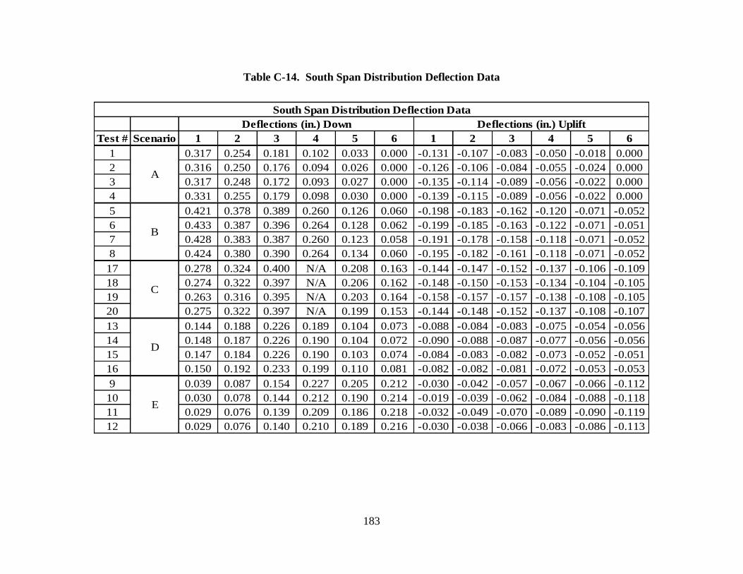
183

Table C-14. South Span Distribution Deflection Data

Test # Scenario 1 2 3 4 5 6 1 2 3 4 5 6

1 0.317 0.254 0.181 0.102 0.033 0.000 -0.131 -0.107 -0.083 -0.050 -0.018 0.000

2 0.316 0.250 0.176 0.094 0.026 0.000 -0.126 -0.106 -0.084 -0.055 -0.024 0.000

3 0.317 0.248 0.172 0.093 0.027 0.000 -0.135 -0.114 -0.089 -0.056 -0.022 0.000

4 0.331 0.255 0.179 0.098 0.030 0.000 -0.139 -0.115 -0.089 -0.056 -0.022 0.000

5 0.421 0.378 0.389 0.260 0.126 0.060 -0.198 -0.183 -0.162 -0.120 -0.071 -0.052

6 0.433 0.387 0.396 0.264 0.128 0.062 -0.199 -0.185 -0.163 -0.122 -0.071 -0.051

7 0.428 0.383 0.387 0.260 0.123 0.058 -0.191 -0.178 -0.158 -0.118 -0.071 -0.052

8 0.424 0.380 0.390 0.264 0.134 0.060 -0.195 -0.182 -0.161 -0.118 -0.071 -0.052

17 0.278 0.324 0.400 N/A 0.208 0.163 -0.144 -0.147 -0.152 -0.137 -0.106 -0.109

18 0.274 0.322 0.397 N/A 0.206 0.162 -0.148 -0.150 -0.153 -0.134 -0.104 -0.105

19 0.263 0.316 0.395 N/A 0.203 0.164 -0.158 -0.157 -0.157 -0.138 -0.108 -0.105

20 0.275 0.322 0.397 N/A 0.199 0.153 -0.144 -0.148 -0.152 -0.137 -0.108 -0.107

13 0.144 0.188 0.226 0.189 0.104 0.073 -0.088 -0.084 -0.083 -0.075 -0.054 -0.056

14 0.148 0.187 0.226 0.190 0.104 0.072 -0.090 -0.088 -0.087 -0.077 -0.056 -0.056

15 0.147 0.184 0.226 0.190 0.103 0.074 -0.084 -0.083 -0.082 -0.073 -0.052 -0.051

16 0.150 0.192 0.233 0.199 0.110 0.081 -0.082 -0.082 -0.081 -0.072 -0.053 -0.053

9 0.039 0.087 0.154 0.227 0.205 0.212 -0.030 -0.042 -0.057 -0.067 -0.066 -0.112

10 0.030 0.078 0.144 0.212 0.190 0.214 -0.019 -0.039 -0.062 -0.084 -0.088 -0.118

11 0.029 0.076 0.139 0.209 0.186 0.218 -0.032 -0.049 -0.070 -0.089 -0.090 -0.119

12 0.029 0.076 0.140 0.210 0.189 0.216 -0.030 -0.038 -0.066 -0.083 -0.086 -0.113

South Span Distribution Deflection Data

Deflections (in.) Down Deflections (in.) Uplift

A

E

B

C

D

184

Table C-15. Highway Speed Test Data

Span Test # 6 5 4 3 2 1 6 5 4 3 2 1

25 11.3 17.6 30.3 54.5 52.0 34.4 0.065 0.099 0.188 0.182 0.209 0.168

26 10.2 16.0 32.7 56.0 50.8 32.3 0.059 0.098 0.189 0.184 0.209 0.169

21 13.1 20.4 38.0 53.4 39.7 28.2 0.075 0.1 0.186 0.225 0.192 0.156

22 12.4 18.3 34.3 50.7 44.8 28.8 0.07 0.094 0.181 0.229 0.204 0.174

23 11.4 17.3 33.6 51.6 42.5 29.5 0.068 0.09 0.176 0.226 0.201 0.169

24 12.9 18.9 34.5 52.6 40.1 28.2 0.074 0.098 0.183 0.224 0.194 0.164

Highway Speed Test Data, Scenario D

South

North

Strains (με) Deflections (in.)

185

Table C-16. North Span Strain Profile Data

Test # Scenario B T C B T C B T C

1 84.0 -12.3 -3.0 60.1 -17.0 -7.0 28.6 -10.0 0.0

2 84.3 -12.2 -5.0 58.8 -17.0 -7.0 28.0 -12.2 0.0

3 84.4 -10.8 -5.0 60.2 -17.8 -7.0 26.8 -11.0 0.0

4 109 -13.7 -7.0 106 -28.7 -15.7 86.1 -21.8 -6.0

5 112 -16.1 -5.0 107 -30.2 -15.7 84.6 -24.2 -8.1

6 109 -16.1 -8.0 105 -28.4 -16.4 84.6 -23.9 -6.0

7 110 -16.5 -7.0 106 -29.4 -17.2 82.8 -23.0 -6.0

16 56.6 -8.0 -4.0 80.8 -24.2 -14.7 96.3 -22.4 -8.0

17 58.9 -7.0 -4.0 82.2 -24.3 -14.4 93.7 -22.2 -9.0

18 57.3 -9.0 -5.0 81.6 -25.4 -14.9 94.7 -25.3 -9.0

19 58.4 -9.0 -5.0 81.4 -25.0 -15.0 96.4 -23.9 -8.0

8 30.0 -4.0 -3.0 42.9 -13.4 -7.9 55.3 -14.6 -5.0

9 29.0 -6.0 -3.0 40.9 -12.8 -9.0 57.0 -15.8 -6.0

10 28.6 -5.0 -3.0 41.3 -13.7 -8.7 54.9 -15.0 -5.0

11 28.8 -5.0 -3.0 42.1 -14.0 -10.3 57.4 -14.5 -5.0

12 8.7 -4.0 -1.0 15.8 -10.0 -5.0 26.9 -7.0 0.0

13 9.4 -3.0 0.0 16.9 -9.0 -4.0 28.7 -8.0 0.0

14 9.3 -3.0 0.0 16.5 -9.0 -3.0 26.9 -7.0 0.0

15 10.2 -3.0 0.0 16.9 -7.0 -4.0 29.4 -7.0 0.0

Girder #

North Span Strain Profile Values (με)

A

B

C

D

E

1 2 3

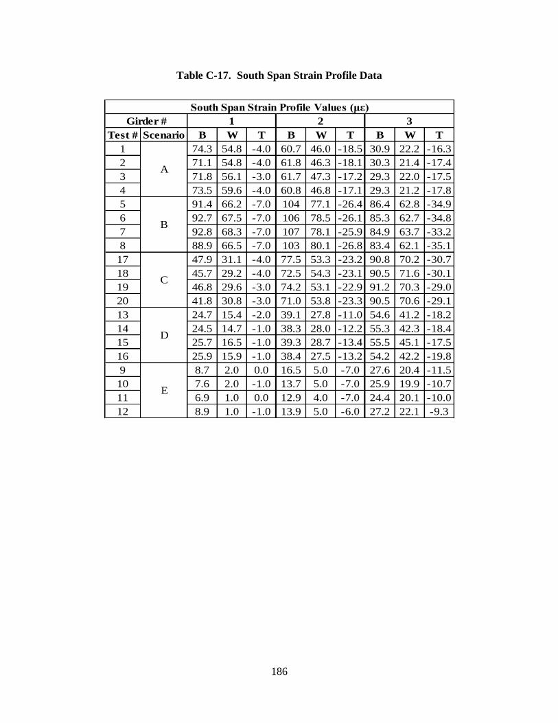
186

Table C-17. South Span Strain Profile Data

Test # Scenario B W T B W T B W T

1 74.3 54.8 -4.0 60.7 46.0 -18.5 30.9 22.2 -16.3

2 71.1 54.8 -4.0 61.8 46.3 -18.1 30.3 21.4 -17.4

3 71.8 56.1 -3.0 61.7 47.3 -17.2 29.3 22.0 -17.5

4 73.5 59.6 -4.0 60.8 46.8 -17.1 29.3 21.2 -17.8

5 91.4 66.2 -7.0 104 77.1 -26.4 86.4 62.8 -34.9

6 92.7 67.5 -7.0 106 78.5 -26.1 85.3 62.7 -34.8

7 92.8 68.3 -7.0 107 78.1 -25.9 84.9 63.7 -33.2

8 88.9 66.5 -7.0 103 80.1 -26.8 83.4 62.1 -35.1

17 47.9 31.1 -4.0 77.5 53.3 -23.2 90.8 70.2 -30.7

18 45.7 29.2 -4.0 72.5 54.3 -23.1 90.5 71.6 -30.1

19 46.8 29.6 -3.0 74.2 53.1 -22.9 91.2 70.3 -29.0

20 41.8 30.8 -3.0 71.0 53.8 -23.3 90.5 70.6 -29.1

13 24.7 15.4 -2.0 39.1 27.8 -11.0 54.6 41.2 -18.2

14 24.5 14.7 -1.0 38.3 28.0 -12.2 55.3 42.3 -18.4

15 25.7 16.5 -1.0 39.3 28.7 -13.4 55.5 45.1 -17.5

16 25.9 15.9 -1.0 38.4 27.5 -13.2 54.2 42.2 -19.8

9 8.7 2.0 0.0 16.5 5.0 -7.0 27.6 20.4 -11.5

10 7.6 2.0 -1.0 13.7 5.0 -7.0 25.9 19.9 -10.7

11 6.9 1.0 0.0 12.9 4.0 -7.0 24.4 20.1 -10.0

12 8.9 1.0 -1.0 13.9 5.0 -6.0 27.2 22.1 -9.3

South Span Strain Profile Values (με)

Girder # 2 3

B

C

D

E

1

A

187

Table C-18. North Span Bearing Rotation Data

1 2 1 2 3 3

Test # Scenario Positive Negative

1 6 N/A -8 N/A 65 -183

2 6 N/A -8 N/A 70 -179

3 6 N/A -9 N/A 69 -180

4 8 7 -10 -3 134 -441

5 7 7 -12 -2 142 -424

6 7 6 -12 -2 136 -440

7 8 6 -11 -2 142 -426

16 3 5 -7 -4 136 -468

17 2 4 -6 -3 137 -469

18 3 4 -6 -3 138 -468

19 2 6 -6 -3 138 -470

8 1 3 -4 -1 69 -247

9 1 2 -4 -1 71 -247

10 1 2 -4 -1 71 -249

11 1 2 -4 -2 69 -247

12 3 2 -2 -3 65 -180

13 3 N/A -2 N/A 64 -180

14 3 N/A -2 N/A 60 -186

15 N/A N/A N/A N/A 67 -180

AbutmentCenter Support

Positive

North Span Bearing Rotations (degrees x 10-4

)

Girder #

Location

D

C

Negative

A

B

E

188

Table C-19. South Span Bearing Rotation Data

1 2 1 2 3 3

Test # Scenario Positive Negative

1 5 NA -5 NA 225 -85

2 5 NA -5 NA 226 -83

3 5 NA -4 NA 223 -84

4 5 NA -5 NA 222 -85

5 4 8 -8 -3 480 -16

6 2 N/A -10 N/A 478 -16

7 4 8 -8 -3 479 -16

8 3 N/A -9 N/A 475 -16

17 N/A 6 N/A -4 472 -14

18 N/A 6 N/A -4 468 -14

19 N/A 6 N/A -4 474 -14

20 N/A N/A N/A N/A N/A N/A

13 N/A 3 N/A -3 248 -76

14 N/A 3 N/A -2 249 -74

15 N/A 3 N/A -2 249 -72

16 N/A 3 N/A -2 248 -74

9 3 3 -3 -3 172 -50

10 3 3 -4 -3 167 -57

11 3 N/A -3 N/A 163 -60

12 4 2 -4 -3 269 -57

E

D

C

B

South Span Bearing Rotations (degrees x 10-4

)

Negative

Location Center Support Abutment

A

Girder #

Positive

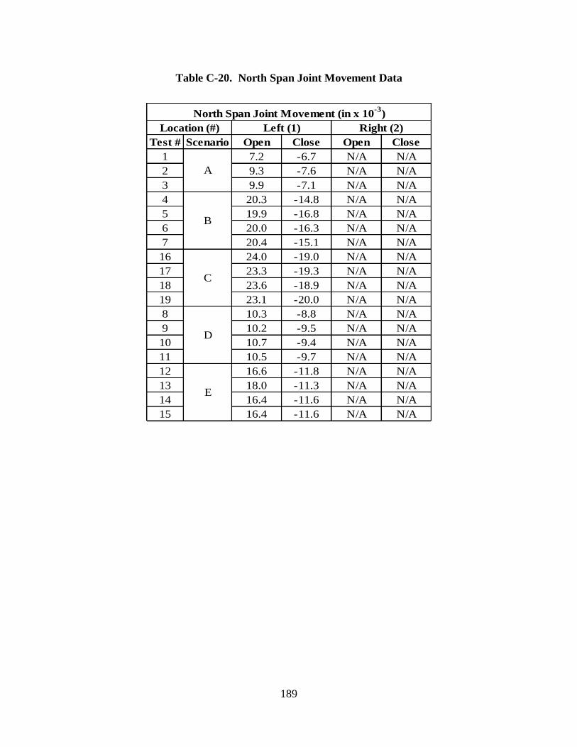
189

Table C-20. North Span Joint Movement Data

Test # Scenario Open Close Open Close

1 7.2 -6.7 N/A N/A

2 9.3 -7.6 N/A N/A

3 9.9 -7.1 N/A N/A

4 20.3 -14.8 N/A N/A

5 19.9 -16.8 N/A N/A

6 20.0 -16.3 N/A N/A

7 20.4 -15.1 N/A N/A

16 24.0 -19.0 N/A N/A

17 23.3 -19.3 N/A N/A

18 23.6 -18.9 N/A N/A

19 23.1 -20.0 N/A N/A

8 10.3 -8.8 N/A N/A

9 10.2 -9.5 N/A N/A

10 10.7 -9.4 N/A N/A

11 10.5 -9.7 N/A N/A

12 16.6 -11.8 N/A N/A

13 18.0 -11.3 N/A N/A

14 16.4 -11.6 N/A N/A

15 16.4 -11.6 N/A N/A

North Span Joint Movement (in x 10-3

)

Location (#)

A

B

C

D

E

Left (1) Right (2)

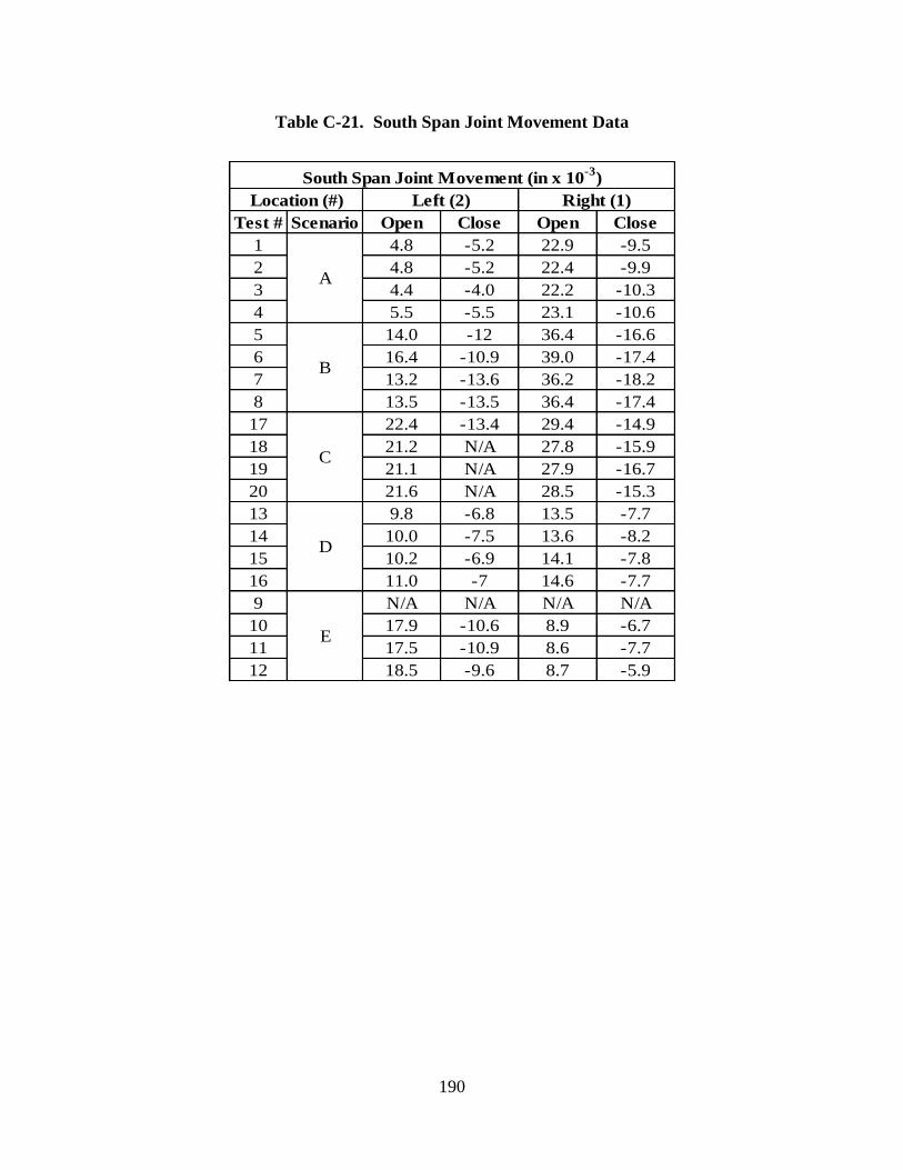
190

Table C-21. South Span Joint Movement Data

Test # Scenario Open Close Open Close

1 4.8 -5.2 22.9 -9.5

2 4.8 -5.2 22.4 -9.9

3 4.4 -4.0 22.2 -10.3

4 5.5 -5.5 23.1 -10.6

5 14.0 -12 36.4 -16.6

6 16.4 -10.9 39.0 -17.4

7 13.2 -13.6 36.2 -18.2

8 13.5 -13.5 36.4 -17.4

17 22.4 -13.4 29.4 -14.9

18 21.2 N/A 27.8 -15.9

19 21.1 N/A 27.9 -16.7

20 21.6 N/A 28.5 -15.3

13 9.8 -6.8 13.5 -7.7

14 10.0 -7.5 13.6 -8.2

15 10.2 -6.9 14.1 -7.8

16 11.0 -7 14.6 -7.7

9 N/A N/A N/A N/A

10 17.9 -10.6 8.9 -6.7

11 17.5 -10.9 8.6 -7.7

12 18.5 -9.6 8.7 -5.9

B

C

D

E

South Span Joint Movement (in x 10-3

)

Location (#)

A

Left (2) Right (1)

191

APPENDIX D: North Span Comparison Plots of Strain and Deflection

Figure D-1. North Span Scenario A Comparison of Strain and Deflection

Figure D-2. North Span Scenario B Comparison of Strain and Deflection

0.000

0.050

0.100

0.150

0.200

0.250

0.300

0.350

0.0

10.0

20.0

30.0

40.0

50.0

60.0

70.0

80.0

90.0

123456

Defl

ecti

on

, in

ch

es

Str

ain

, m

icro

stra

in

Girder Number

North Span, Scenario A

Strain

Deflection

0.000

0.050

0.100

0.150

0.200

0.250

0.300

0.350

0.400

0.450

0.0

20.0

40.0

60.0

80.0

100.0

120.0

123456

Defl

ecti

on

, in

ch

es

Str

ain

, m

icro

stra

in

Girder Number

North Span, Scenario B

Strain

Deflection

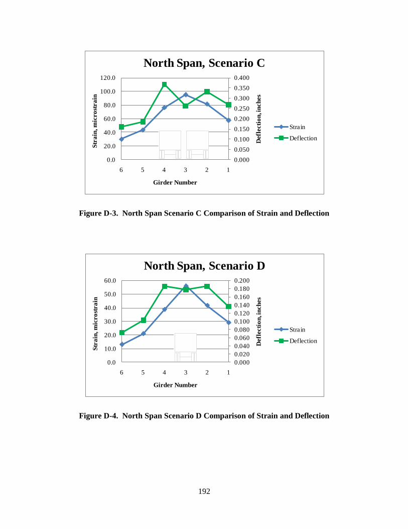
192

Figure D-3. North Span Scenario C Comparison of Strain and Deflection

Figure D-4. North Span Scenario D Comparison of Strain and Deflection

0.000

0.050

0.100

0.150

0.200

0.250

0.300

0.350

0.400

0.0

20.0

40.0

60.0

80.0

100.0

120.0

123456

Defl

ecti

on

, in

ch

es

Str

ain

, m

icro

stra

in

Girder Number

North Span, Scenario C

Strain

Deflection

0.000

0.020

0.040

0.060

0.080

0.100

0.120

0.140

0.160

0.180

0.200

0.0

10.0

20.0

30.0

40.0

50.0

60.0

123456

Defl

ecti

on

, in

ch

es

Str

ain

, m

icro

stra

in

Girder Number

North Span, Scenario D

Strain

Deflection

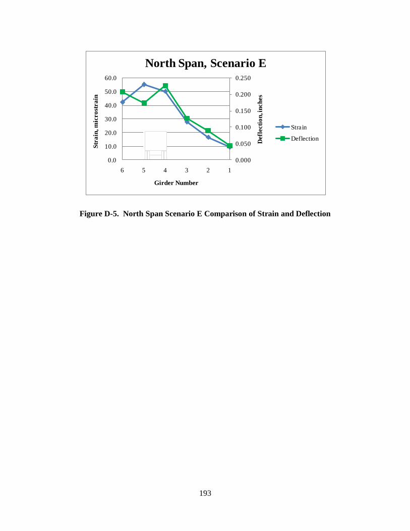
193

Figure D-5. North Span Scenario E Comparison of Strain and Deflection

0.000

0.050

0.100

0.150

0.200

0.250

0.0

10.0

20.0

30.0

40.0

50.0

60.0

123456

Defl

ecti

on

, in

ch

es

Str

ain

, m

icro

stra

in

Girder Number

North Span, Scenario E

Strain

Deflection

194

APPENDIX E: AASHTO Distribution Factor Equation Calculations

Given:

S = 90 in. L = 137 ft. Agirder = 72.62 in2 Igirder = 42,590 in

4

tslab = 8.625 in. de = 7 in. Esteel = 29000 ksi f’c = 4000 psi

eg= 43.83 in.

Figure E-1. Bridge Cross Section at Four Tenths of Span Length

Calculations:

90 7S=7'-6" de=7"

40eg=43.83"

195

The distribution factor for the exterior girder with one lane loaded, gext one, is calculated using the

lever rule, which is shown in Appendix F.

This distribution factor is then compared with the value calculated using the lever rule, and the

lesser of the two values is chosen.

196

APPENDIX F: Distribution Factor Calculation Using Lever Rule

Given:

de = 7 in. S = 90 in.

Figure F-1. Cross Section Used for Lever Rule Calculation

Assumptions:

Deck hinges over first interior girder

Deck acts as a rigid body

Each wheel line applies half of load, P

First wheel line is positioned 2 feet from barrier rail

Axle spacing is 6’-0”

Calculations:

This distribution factor, g, is then multiplied by the appropriate multiple presence factor.

2472

90 7

6'-0" 2'-0"

S=7'-6" de=7"

Hinge

P/2 P/2

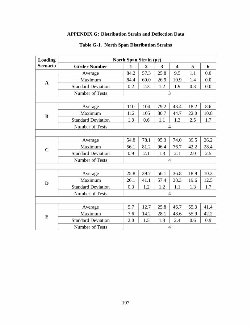
197

APPENDIX G: Distribution Strain and Deflection Data

Table G-1. North Span Distribution Strains

Loading

Scenario

North Span Strain (με)

Girder Number 1 2 3 4 5 6

A

Average 84.2 57.3 25.8 9.5 1.1 0.0

Maximum 84.4 60.0 26.9 10.9 1.4 0.0

Standard Deviation 0.2 2.3 1.2 1.9 0.3 0.0

Number of Tests 3

B

Average 110 104 79.2 43.4 18.2 8.6

Maximum 112 105 80.7 44.7 22.0 10.8

Standard Deviation 1.3 0.6 1.1 1.3 2.5 1.7

Number of Tests 4

C

Average 54.8 78.1 95.3 74.0 39.5 26.2

Maximum 56.1 81.2 96.4 76.7 42.2 28.4

Standard Deviation 0.9 2.1 1.3 2.1 2.0 2.5

Number of Tests 4

D

Average 25.8 39.7 56.1 36.8 18.9 10.3

Maximum 26.1 41.1 57.4 38.3 19.6 12.5

Standard Deviation 0.3 1.2 1.2 1.1 1.3 1.7

Number of Tests 4

E

Average 5.7 12.7 25.8 46.7 55.3 41.4

Maximum 7.6 14.2 28.1 48.6 55.9 42.2

Standard Deviation 2.0 1.5 1.8 2.4 0.6 0.9

Number of Tests 4

198

Table G-2. North Span Distribution Deflections

Loading

Scenario

North Span Deflection (in)

Girder Number 1 2 3 4 5 6

A

Average 0.317 0.249 0.143 0.091 0.032 0.000

Maximum 0.325 0.253 0.146 0.094 0.035 0.000

Standard Deviation 0.009 0.004 0.004 0.004 0.003 0.000

Number of Tests 3

B

Average 0.409 0.390 0.262 0.272 0.124 0.060

Maximum 0.428 0.394 0.269 0.279 0.133 0.069

Standard Deviation 0.013 0.003 0.005 0.005 0.006 0.007

Number of Tests 4

C

Average 0.260 0.328 0.261 0.368 0.185 0.158

Maximum 0.268 0.333 0.264 0.371 0.188 0.161

Standard Deviation 0.005 0.003 0.003 0.004 0.004 0.005

Number of Tests 4

D

Average 0.134 0.185 0.177 0.184 0.101 0.068

Maximum 0.138 0.186 0.180 0.189 0.105 0.072

Standard Deviation 0.005 0.002 0.002 0.004 0.003 0.004

Number of Tests 4

E

Average 0.035 0.084 0.126 0.227 0.172 0.206

Maximum 0.040 0.089 0.130 0.234 0.174 0.217

Standard Deviation 0.005 0.005 0.004 0.006 0.002 0.008

Number of Tests 4

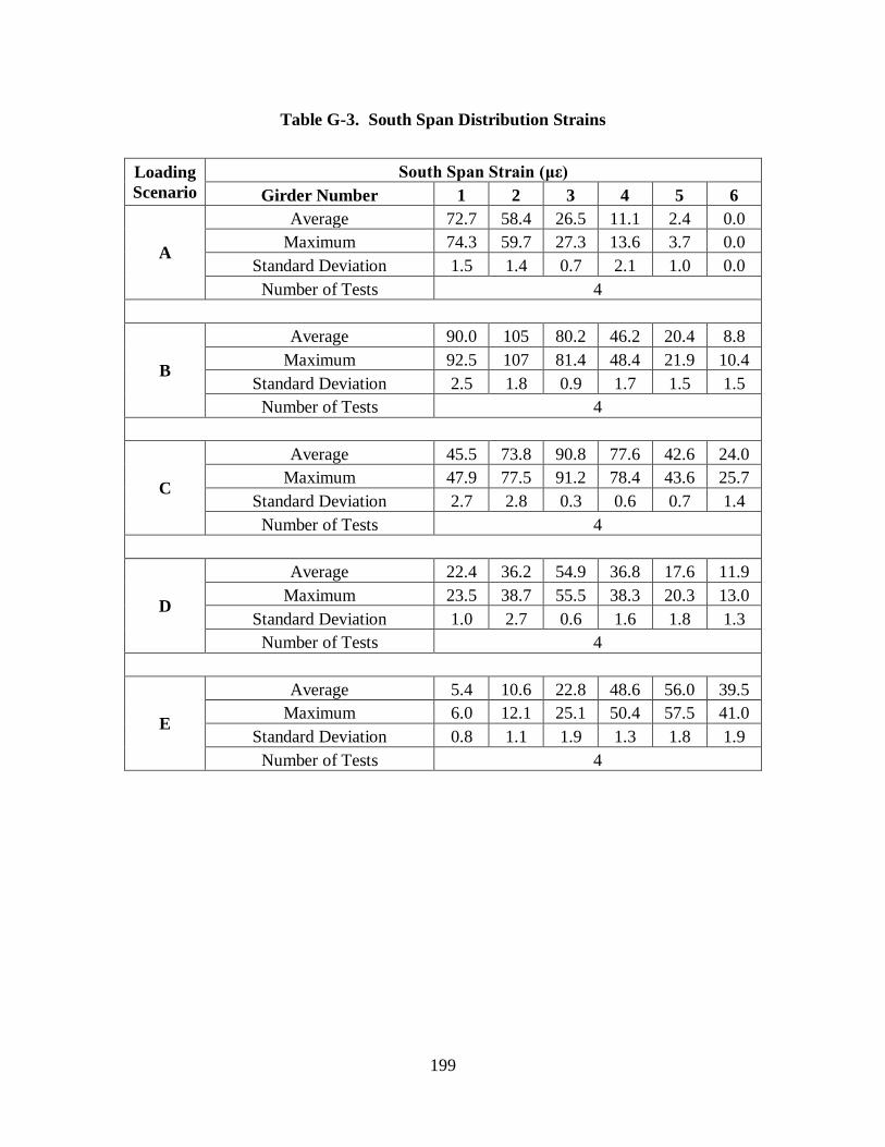
199

Table G-3. South Span Distribution Strains

Loading

Scenario

South Span Strain (με)

Girder Number 1 2 3 4 5 6

A

Average 72.7 58.4 26.5 11.1 2.4 0.0

Maximum 74.3 59.7 27.3 13.6 3.7 0.0

Standard Deviation 1.5 1.4 0.7 2.1 1.0 0.0

Number of Tests 4

B

Average 90.0 105 80.2 46.2 20.4 8.8

Maximum 92.5 107 81.4 48.4 21.9 10.4

Standard Deviation 2.5 1.8 0.9 1.7 1.5 1.5

Number of Tests 4

C

Average 45.5 73.8 90.8 77.6 42.6 24.0

Maximum 47.9 77.5 91.2 78.4 43.6 25.7

Standard Deviation 2.7 2.8 0.3 0.6 0.7 1.4

Number of Tests 4

D

Average 22.4 36.2 54.9 36.8 17.6 11.9

Maximum 23.5 38.7 55.5 38.3 20.3 13.0

Standard Deviation 1.0 2.7 0.6 1.6 1.8 1.3

Number of Tests 4

E

Average 5.4 10.6 22.8 48.6 56.0 39.5

Maximum 6.0 12.1 25.1 50.4 57.5 41.0

Standard Deviation 0.8 1.1 1.9 1.3 1.8 1.9

Number of Tests 4

200

Table G-4. South Span Distribution Deflections

Loading

Scenario

South Span Deflection (in)

Girder Number 1 2 3 4 5 6

A

Average 0.320 0.252 0.177 0.097 0.029 0.000

Maximum 0.331 0.255 0.181 0.102 0.033 0.000

Standard Deviation 0.007 0.003 0.004 0.004 0.003 0.000

Number of Tests 4

B

Average 0.427 0.382 0.391 0.262 0.128 0.060

Maximum 0.433 0.387 0.396 0.264 0.134 0.062

Standard Deviation 0.005 0.004 0.004 0.002 0.005 0.002

Number of Tests 4

C

Average 0.273 0.321 0.397 0.301* 0.204 0.161

Maximum 0.278 0.324 0.400 N/A 0.208 0.164

Standard Deviation 0.007 0.003 0.002 N/A 0.004 0.005

Number of Tests 4

D

Average 0.147 0.188 0.228 0.192 0.105 0.075

Maximum 0.150 0.192 0.233 0.199 0.110 0.081

Standard Deviation 0.003 0.003 0.004 0.005 0.003 0.004

Number of Tests 4

E

Average 0.032 0.079 0.144 0.215 0.193 0.215

Maximum 0.039 0.087 0.154 0.227 0.205 0.218

Standard Deviation 0.005 0.005 0.007 0.008 0.009 0.003

Number of Tests 4

* Estimated Value

201

APPENDIX H: Highway Speed Test Data and Dynamic Load Allowance

Table H-1. North Span Dynamic Response Data

North Span

Strain (με)

Girder 1 2 3 4 5 6

Average 33.4 51.4 55.2 31.5 16.8 10.7

Maximum 34.4 52.0 56.0 32.7 17.6 11.3

Standard Dev. 1.4 0.9 1.1 1.7 1.1 0.8

Deflection (in)

Average 0.169 0.209 0.183 0.189 0.099 0.062

Maximum 0.169 0.209 0.184 0.189 0.099 0.065

Standard Dev. 0.001 0.000 0.001 0.001 0.001 0.004

Number of Tests 2

Table H-2. South Span Dynamic Response Data

South Span

Strain (με)

Girder 1 2 3 4 5 6

Average 28.7 41.8 52.1 35.1 18.7 12.4

Maximum 29.5 44.8 53.4 38.0 20.4 13.1

Standard Dev. 0.6 2.4 1.2 2.0 1.3 0.8

Deflection (in)

Average 0.166 0.198 0.226 0.182 0.096 0.072

Maximum 0.174 0.204 0.229 0.186 0.100 0.075

Standard Dev. 0.008 0.006 0.002 0.004 0.004 0.003

Number of Tests 4

202

Table H-3. Calculated Dynamic Load Allowance

Dynamic Load Allowance, IM

Span Response 1 2 3 4 5 6

North Strain 0.15 0.23 -0.02 -0.19 -0.20 -0.17

Deflection 0.23 0.12 0.03 0.01 -0.04 -0.14

South Strain 0.14 0.08 -0.05 -0.13 -0.14 -0.15

Deflection 0.11 0.05 -0.01 -0.06 -0.11 -0.11

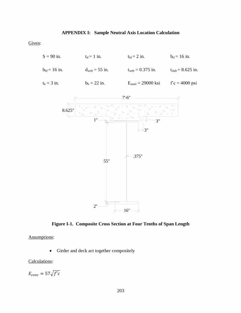
203

APPENDIX I: Sample Neutral Axis Location Calculation

Given:

S = 90 in. ttf = 1 in. tbf = 2 in. btf = 16 in.

bbf = 16 in. dweb = 55 in. tweb = 0.375 in. tslab = 8.625 in.

th = 3 in. bh = 22 in. Esteel = 29000 ksi f’c = 4000 psi

Figure I-1. Composite Cross Section at Four Tenths of Span Length

Assumptions:

Girder and deck act together compositely

Calculations:

3"

3"

27'-6"

8

1

55

216

55"

2"16"

1"

8.625"

.375"

204

This represents the neutral axis location of the non-composite girder measured from the

bottom of the bottom flange.

This represents the neutral axis location for the composite girder measured from the

bottom of the bottom flange.

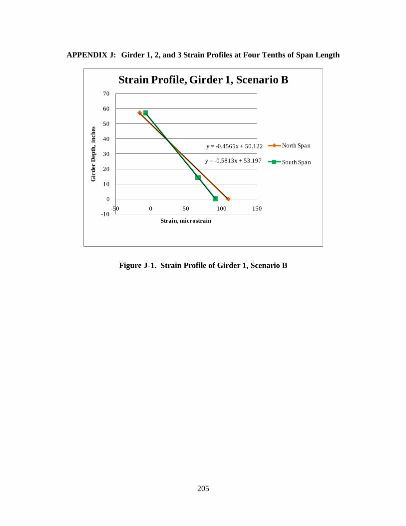
205

APPENDIX J: Girder 1, 2, and 3 Strain Profiles at Four Tenths of Span Length

Figure J-1. Strain Profile of Girder 1, Scenario B

y = -0.4565x + 50.122

y = -0.5813x + 53.197

-10

0

10

20

30

40

50

60

70

-50 0 50 100 150

Gir

der D

ep

th,

inch

es

Strain, microstrain

Strain Profile, Girder 1, Scenario B

North Span

South Span

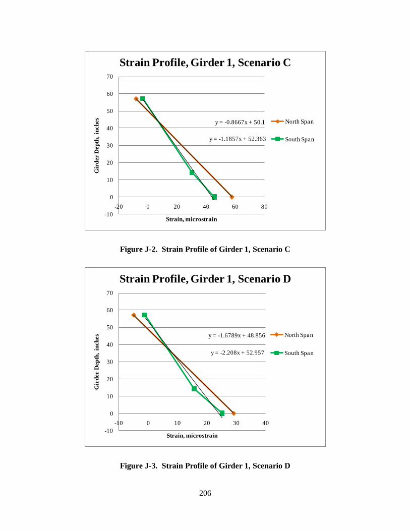
206

Figure J-2. Strain Profile of Girder 1, Scenario C

Figure J-3. Strain Profile of Girder 1, Scenario D

y = -0.8667x + 50.1

y = -1.1857x + 52.363

-10

0

10

20

30

40

50

60

70

-20 0 20 40 60 80

Gir

der D

ep

th,

inch

es

Strain, microstrain

Strain Profile, Girder 1, Scenario C

North Span

South Span

y = -1.6789x + 48.856

y = -2.208x + 52.957

-10

0

10

20

30

40

50

60

70

-10 0 10 20 30 40

Gir

der D

ep

th,

inch

es

Strain, microstrain

Strain Profile, Girder 1, Scenario D

North Span

South Span

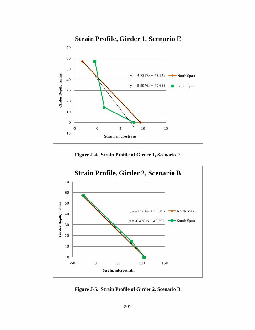
207

Figure J-4. Strain Profile of Girder 1, Scenario E

Figure J-5. Strain Profile of Girder 2, Scenario B

y = -4.5257x + 42.542

y = -5.5976x + 40.663

-10

0

10

20

30

40

50

60

70

-5 0 5 10 15

Gir

der D

ep

th,

inch

es

Strain, microstrain

Strain Profile, Girder 1, Scenario E

North Span

South Span

y = -0.4239x + 44.886

y = -0.4281x + 46.297

0

10

20

30

40

50

60

70

-50 0 50 100 150

Gir

der D

ep

th,

inch

es

Strain, microstrain

Strain Profile, Girder 2, Scenario B

North Span

South Span

208

Figure J-6. Strain Profile of Girder 2, Scenario C

Figure J-7. Strain Profile of Girder 2, Scenario D

y = -0.5389x + 43.92

y = -0.5823x + 44.088

-10

0

10

20

30

40

50

60

70

-40 -20 0 20 40 60 80 100

Gir

der D

ep

th,

inch

es

Strain, microstrain

Strain Profile, Girder 2, Scenario C

North Span

South Span

y = -1.0359x + 43.299

y = -1.1025x + 43.812

-10

0

10

20

30

40

50

60

70

-20 0 20 40 60

Gir

der D

ep

th,

inch

es

Strain, microstrain

Strain Profile, Girder 2, Scenario D

North Span

South Span

209

Figure J-8. Strain Profile of Girder 2, Scenario E

Figure J-9. Strain Profile of Girder 3, Scenario B

y = -2.266x + 37.423

y = -2.765x + 35.101

-10

0

10

20

30

40

50

60

70

-15 -10 -5 0 5 10 15 20

Gir

der D

ep

th,

inch

es

Strain, microstrain

Strain Profile, Girder 2, Scenario E

North Span

South Span

y = -0.5314x + 44.916

y = -0.4679x + 41.508

0

10

20

30

40

50

60

70

-50 0 50 100

Gir

der D

ep

th,

inch

es

Strain, microstrain

Strain Profile, Girder 3, Scenario B

North Span

South Span

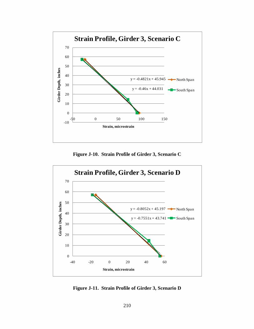
210

Figure J-10. Strain Profile of Girder 3, Scenario C

Figure J-11. Strain Profile of Girder 3, Scenario D

y = -0.4821x + 45.945

y = -0.46x + 44.031

-10

0

10

20

30

40

50

60

70

-50 0 50 100 150

Gir

der D

ep

th,

inch

es

Strain, microstrain

Strain Profile, Girder 3, Scenario C

North Span

South Span

y = -0.8052x + 45.197

y = -0.7551x + 43.741

0

10

20

30

40

50

60

70

-40 -20 0 20 40 60

Gir

der D

ep

th,

inch

es

Strain, microstrain

Strain Profile, Girder 3, Scenario D

North Span

South Span

211

Figure J-12. Strain Profile of Girder 3, Scenario E

y = -1.6261x + 45.461

y = -1.5043x + 42.157

0

10

20

30

40

50

60

70

-20 -10 0 10 20 30

Gir

der D

ep

th,

inch

es

Strain, microstrain

Strain Profile, Girder 3, Scenario E

North Span

South Span

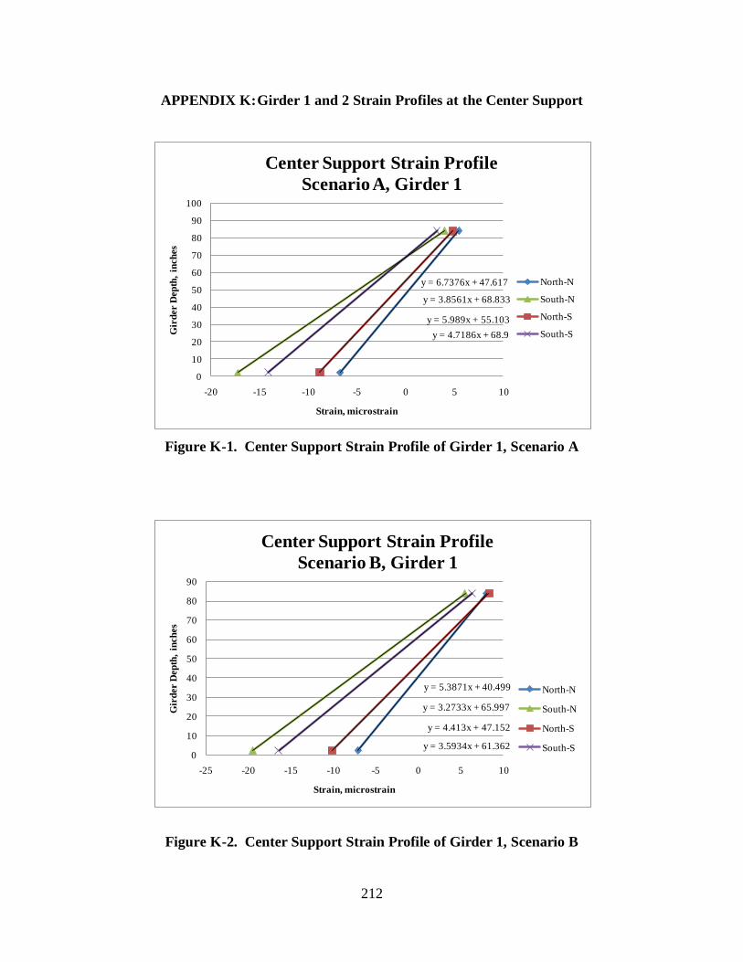
212

APPENDIX K: Girder 1 and 2 Strain Profiles at the Center Support

Figure K-1. Center Support Strain Profile of Girder 1, Scenario A

Figure K-2. Center Support Strain Profile of Girder 1, Scenario B

y = 6.7376x + 47.617

y = 3.8561x + 68.833

y = 5.989x + 55.103

y = 4.7186x + 68.9

0

10

20

30

40

50

60

70

80

90

100

-20 -15 -10 -5 0 5 10

Gir

der D

ep

th,

inch

es

Strain, microstrain

Center Support Strain Profile

Scenario A, Girder 1

North-N

South-N

North-S

South-S

y = 5.3871x + 40.499

y = 3.2733x + 65.997

y = 4.413x + 47.152

y = 3.5934x + 61.3620

10

20

30

40

50

60

70

80

90

-25 -20 -15 -10 -5 0 5 10

Gir

der D

ep

th,

inch

es

Strain, microstrain

Center Support Strain Profile

Scenario B, Girder 1

North-N

South-N

North-S

South-S

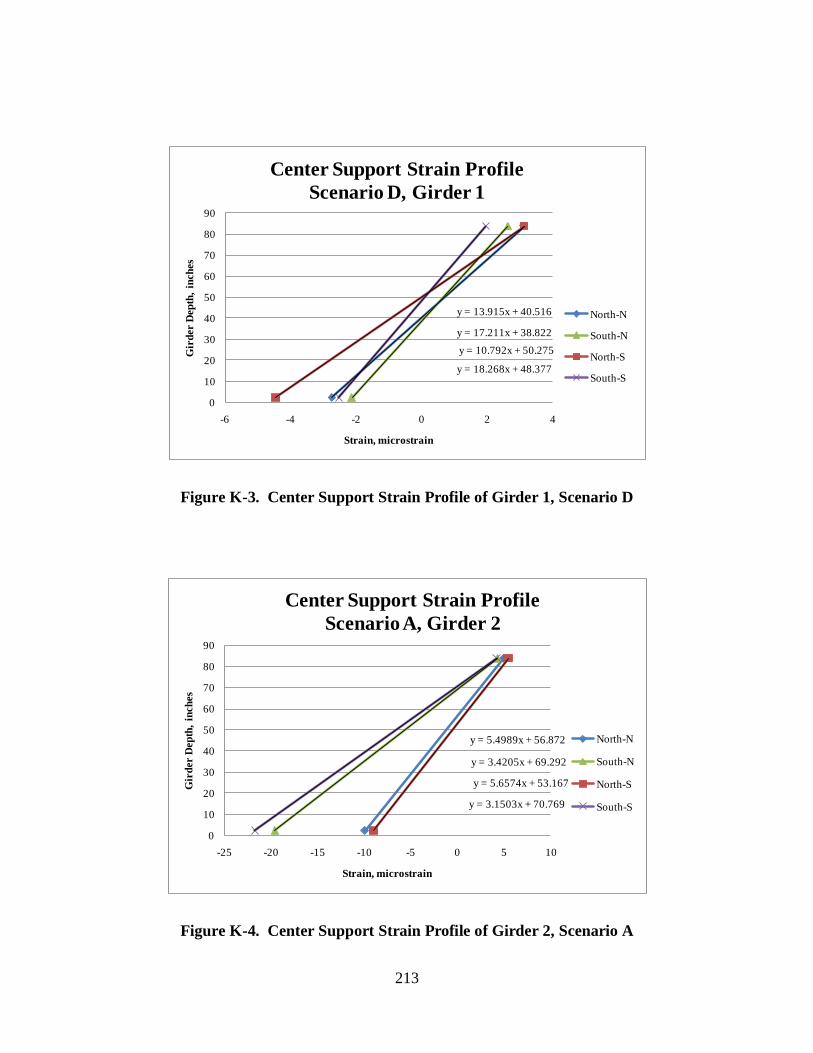
213

Figure K-3. Center Support Strain Profile of Girder 1, Scenario D

Figure K-4. Center Support Strain Profile of Girder 2, Scenario A

y = 13.915x + 40.516

y = 17.211x + 38.822

y = 10.792x + 50.275

y = 18.268x + 48.377

0

10

20

30

40

50

60

70

80

90

-6 -4 -2 0 2 4

Gir

der D

ep

th,

inch

es

Strain, microstrain

Center Support Strain Profile

Scenario D, Girder 1

North-N

South-N

North-S

South-S

y = 5.4989x + 56.872

y = 3.4205x + 69.292

y = 5.6574x + 53.167

y = 3.1503x + 70.769

0

10

20

30

40

50

60

70

80

90

-25 -20 -15 -10 -5 0 5 10

Gir

der D

ep

th,

inch

es

Strain, microstrain

Center Support Strain Profile

Scenario A, Girder 2

North-N

South-N

North-S

South-S

214

Figure K-5. Center Support Strain Profile of Girder 2, Scenario B

Figure K-6. Center Support Strain Profile of Girder 2, Scenario D

y = 3.2473x + 51.771

y = 2.0135x + 67.187

y = 3.3064x + 51.35

y = 1.91x + 67.43

0

10

20

30

40

50

60

70

80

90

100

-40 -30 -20 -10 0 10 20

Gir

der D

ep

th,

inch

es

Strain, microstrain

Center Support Strain Profile

Scenario B, Girder 2

North-N

South-N

North-S

South-S

y = 9.1341x + 45.18

y = 5.2998x + 65.451

y = 9.7612x + 41.051

y = 4.5166x + 67.402

0

10

20

30

40

50

60

70

80

90

100

-20 -15 -10 -5 0 5 10

Gir

der D

ep

th,

inch

es

Strain, microstrain

Center Support Strain Profile

Scenario D, Girder 2

North-N

South-N

North-S

South-S

215

APPENDIX L: Pseudo-Static Bearing Rotation Data

Table L-1. Bearing Rotations, Scenario A

Location Abutment Abutment

Girder Number 1 2 3 1 2 3

Average 6 N/A 68 5 N/A 224

Maximum 6 N/A 70 5 N/A 226

Standard Deviation 0.1 N/A 2.8 0.3 N/A 1.6

Average -9 N/A -181 -5 N/A -84

Maximum -9 N/A -183 -5 N/A -85

Standard Deviation 0.5 N/A 2.0 0.3 N/A 0.7

Number of Tests

Loading Scenario A

North Span

Pos. Rotation (degrees x 10-4

)

South Span

Center Support Center Support

3 4

Neg. Rotation (degrees x 10-4

)

Table L-2. Bearing Rotations, Scenario B

Location Abutment Abutment

Girder Number 1 2 3 1 2 3

Average 7 6 138 3 8 478

Maximum 8 7 142 4 8 480

Standard Deviation 0.6 0.5 3.7 1.0 0.0 2.2

Average -12 -2 -433 -9 -3 -159

Maximum -12 -3 -441 -10 -3 -164

Standard Deviation 0.4 0.5 9.0 1.1 0.1 3.7

Number of Tests 4 2 4

Loading Scenario B

North Span

Pos. Rotation (degrees x 10-4

)

Neg. Rotation (degrees x 10-4

)

4

South Span

Center Support Center Support

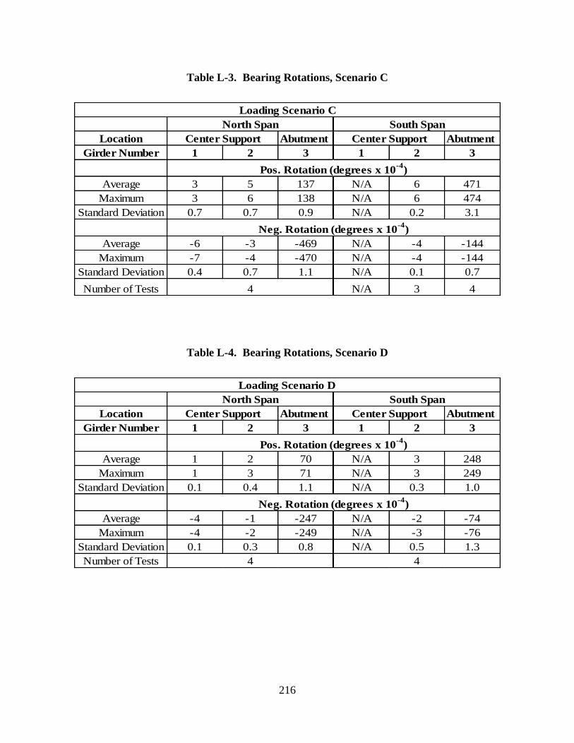
216

Table L-3. Bearing Rotations, Scenario C

Location Abutment Abutment

Girder Number 1 2 3 1 2 3

Average 3 5 137 N/A 6 471

Maximum 3 6 138 N/A 6 474

Standard Deviation 0.7 0.7 0.9 N/A 0.2 3.1

Average -6 -3 -469 N/A -4 -144

Maximum -7 -4 -470 N/A -4 -144

Standard Deviation 0.4 0.7 1.1 N/A 0.1 0.7

Number of Tests N/A 3 4

Center Support Center Support

Pos. Rotation (degrees x 10-4

)

Neg. Rotation (degrees x 10-4

)

4

South Span

Loading Scenario C

North Span

Table L-4. Bearing Rotations, Scenario D

Location Abutment Abutment

Girder Number 1 2 3 1 2 3

Average 1 2 70 N/A 3 248

Maximum 1 3 71 N/A 3 249

Standard Deviation 0.1 0.4 1.1 N/A 0.3 1.0

Average -4 -1 -247 N/A -2 -74

Maximum -4 -2 -249 N/A -3 -76

Standard Deviation 0.1 0.3 0.8 N/A 0.5 1.3

Number of Tests

Neg. Rotation (degrees x 10-4

)

Center Support Center Support

Loading Scenario D

North Span South Span

4 4

Pos. Rotation (degrees x 10-4

)

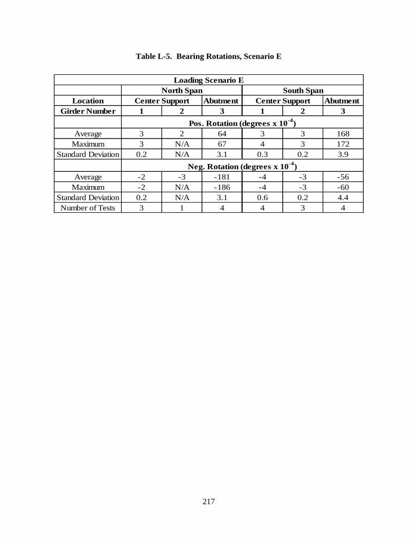
217

Table L-5. Bearing Rotations, Scenario E

Location Abutment Abutment

Girder Number 1 2 3 1 2 3

Average 3 2 64 3 3 168

Maximum 3 N/A 67 4 3 172

Standard Deviation 0.2 N/A 3.1 0.3 0.2 3.9

Average -2 -3 -181 -4 -3 -56

Maximum -2 N/A -186 -4 -3 -60

Standard Deviation 0.2 N/A 3.1 0.6 0.2 4.4

Number of Tests 3 1 4 4 3 4

Neg. Rotation (degrees x 10-4

)

Loading Scenario E

South Span

Center Support Center Support

North Span

Pos. Rotation (degrees x 10-4

)

218

APPENDIX M: Comparison of LVDT Base Rotations with Bearing Rotations

Figure M-1. North Abutment Rotation Comparisons, Scenario A

Figure M-2. North Abutment Rotation Comparisons, Scenario B

1 103

0

1 103

2 103

3 103

Marker

Time, 0.01 seconds

Mar

ker

Marker

time

0 100 2000.02

0.01

0

0.01

Left Side LVDT

Inclinometer

North Abutment Girder 3 Bearing Rotation Comparison, Scenario A

Truck Position Along Bridge, feet

Rota

tion, deg

rees

0 100 2000.06

0.04

0.02

0

0.02

Left Side LVDT

Inclinometer

North Abutment Girder 3 Bearing Rotation Comparison, Scenario B

Truck Position Along Bridge, feet

Rota

tion, deg

rees

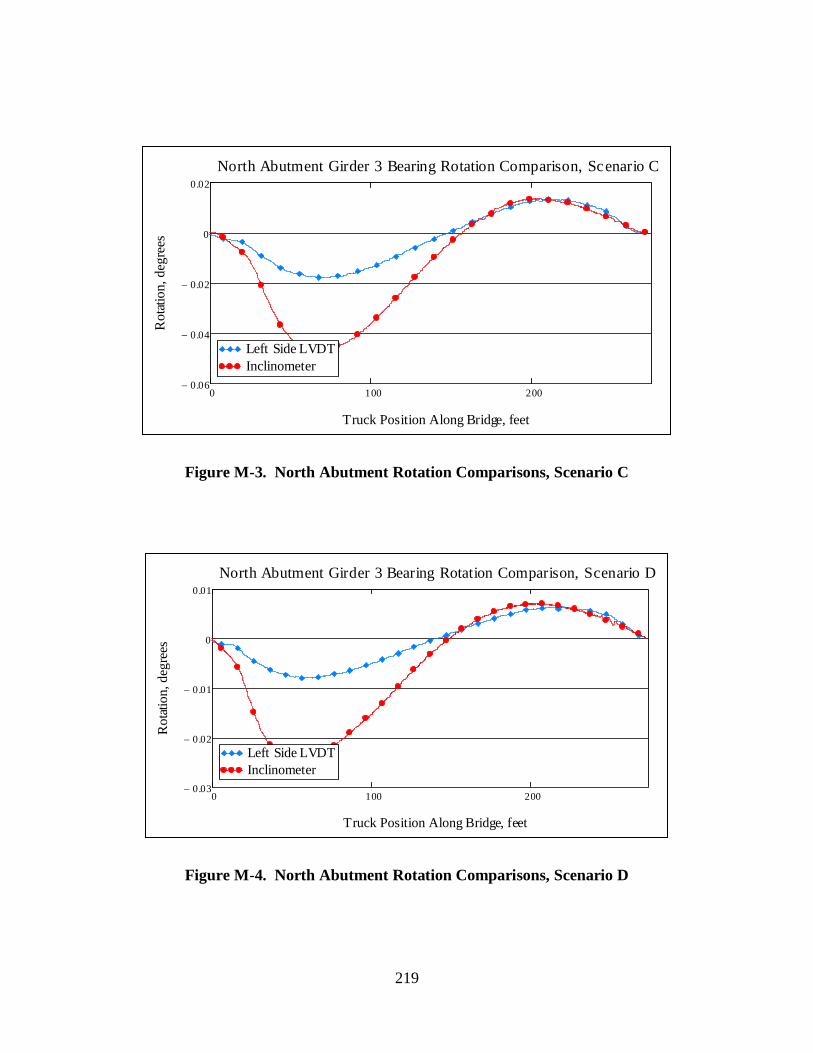
219

Figure M-3. North Abutment Rotation Comparisons, Scenario C

Figure M-4. North Abutment Rotation Comparisons, Scenario D

0 100 2000.06

0.04

0.02

0

0.02

Left Side LVDT

Inclinometer

North Abutment Girder 3 Bearing Rotation Comparison, Scenario C

Truck Position Along Bridge, feet

Ro

tatio

n,

deg

rees

0 100 2000.03

0.02

0.01

0

0.01

Left Side LVDT

Inclinometer

North Abutment Girder 3 Bearing Rotation Comparison, Scenario D

Truck Position Along Bridge, feet

Ro

tatio

n, d

egre

es

220

Figure M-5. North Abutment Rotation Comparisons, Scenario E

Figure M-6. South Abutment Rotation Comparisons, Scenario A

0 100 2000.02

0.01

0

0.01

Left Side LVDT

Inclinometer

North Abutment Girder 3 Bearing Rotation Comparison, Scenario E

Truck Position Along Bridge, feet

Ro

tatio

n,

deg

rees

0 2 103

4 103

6 103

8 103

500

0

500

1 103

1.5 103

2 103

Marker

Time, 0.01 seconds

Mar

ker

Marker

time

0 100 2000.03

0.02

0.01

0

0.01

Right Side LVDT

Left Side LVDT

Inclinometer

South Abutment Girder 3 Bearing Rotation Comparison, Scenario A

Truck Position Along Bridge, feet

Ro

tatio

n,

deg

rees

MS 3621

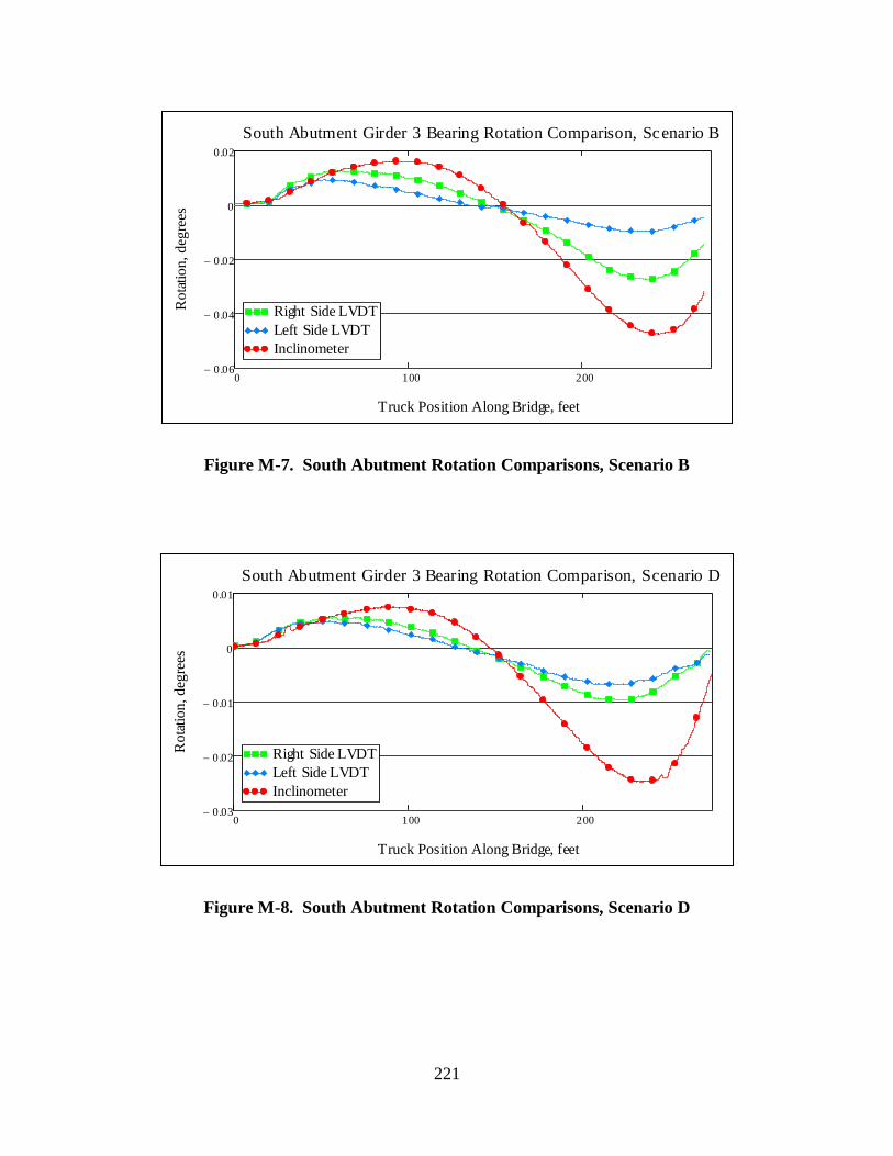
221

Figure M-7. South Abutment Rotation Comparisons, Scenario B

Figure M-8. South Abutment Rotation Comparisons, Scenario D

1 103

0

1 103

2 103

3 103

Marker

Time, 0.01 seconds

Mar

ker

Marker

time

0 100 2000.06

0.04

0.02

0

0.02

Right Side LVDT

Left Side LVDT

Inclinometer

South Abutment Girder 3 Bearing Rotation Comparison, Scenario B

Truck Position Along Bridge, feet

Ro

tatio

n,

deg

rees

0 100 2000.03

0.02

0.01

0

0.01

Right Side LVDT

Left Side LVDT

Inclinometer

South Abutment Girder 3 Bearing Rotation Comparison, Scenario D

Truck Position Along Bridge, feet

Ro

tatio

n, d

egre

es

222

Figure M-9. South Abutment Rotation Comparisons, Scenario E

0

1 103

2 103

3 103

Marker

Time, 0.01 seconds

Mar

ker

Marker

time

0 100 2000.02

0.01

0

0.01

Right Side LVDT

Left Side LVDT

Inclinometer

South Abutment Girder 3 Bearing Rotation Comparison, Scenario E

Truck Position Along Bridge, feet

Rota

tion, deg

rees