Little’s Theorem Examples Courtesy of: Dr. Abdul Waheed (previous instructor at COE)

Little’s Theorem Examples

Courtesy of:Dr. Abdul Waheed

(previous instructor at COE)

Term 032 3-4-2 COE540-Abdul Waheed

Example # 1: Little’s Theorem Consider a network of transmission lines

Packets arrive at n different nodes with corresponding rates 1, …, n

If N is the average total number of packets inside the network, then determine the average delay per packet (T), regardless of the packet length distribution and method of routing packet

Applying Little’s theorem:

If Ni and Ti are average number in the system and average delay of packets arriving at node i, respectively, then Ni = iTi

n

i i

NT

1


Example # 2 A packet arrives at a transmission line every K seconds

The first packet arriving at time 0 All packets have equal length and require K seconds for

transmission where < 1 The processing and propagation delay per packet is P seconds Determine average number in the system N

Solution: The arrival rate here is = 1/K Since packets arrive at regular rate (equal inter-arrival times),

there is no delay for queuing time T a packets spends in the system (including propagation delay) is: T = K + P

Applying Little’s theorem to find time average # in system:N = T = + P/K Here, the # in system N(t) is a deterministic function of time In this case, N(t) does not converge but Little’s theorem holds

with N viewed as a time average

K<K+P<2K


Example # 3 Consider a window flow control system

Window size is W for each session Arrival rate of packets into the system for each session = Apply Little’s theorem to analyze impact of W on and delay

T Applying Little’s theorem:

Since, # of packets in the system is never more than W, thereforeW > T

If congestion builds up in the system T increases and must eventually decrease

Next, the network is congested and capable of delivering packets per unit time for each session. Assuming delays for ACKs to be negligible relative to forward packets and W T

Increasing W in this case only result in increasing delay T without appreciably changing


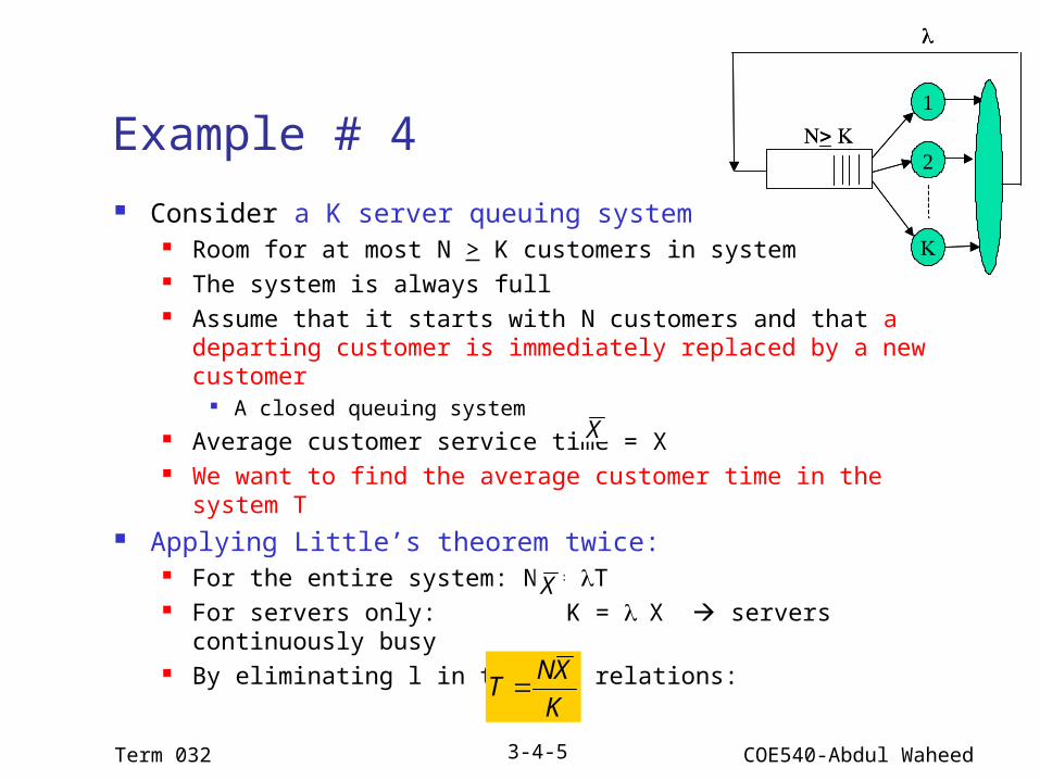
Example # 4

Consider a K server queuing system Room for at most N > K customers in system The system is always full Assume that it starts with N customers and that a

departing customer is immediately replaced by a new customer

A closed queuing system Average customer service time = X We want to find the average customer time in the system T

Applying Little’s theorem twice: For the entire system: N = T For servers only: K = X servers continuously

busy By eliminating l in the two relations:

X

K

XNT

X


Example # 4 (Cont’d) Now consider same system under different arrival

assumptions Customers arrive at rate but are blocked (and lost) from the

system if they find the system full Then the number of servers that may be busy are less than K Let K be the average number of busy servers Let be the proportion of customers that are blocked from

entering the system Applying Little’s theorem to the servers of the system:

Effective arrival rate = (1 – ) Then average number of busy servers are given as: K = (1 – )X Which gives:

Since, K < K, we obtain a lower bound on blocking probability as:

K

K

K X

X

K

1

X

K

1


Example # 5: A Polling System Consider a transmission line:

Serves m packet streams (i.e., m users) in round-robin cycles In each cycle, some packets of user 1 are transmitted

followed by some packets of user 2, and son on until finally packets of user m are transmitted

An overhead period of average length Ai precedes the transmission of the packets of user i in each cycle

The arrival rate and average transmission time of the packets of user i are i and Xi respectively

If A = A1 + A2 + … + Am, determine average cycle length L Applying Little’s theorem:

Fraction of time the transmission line is busy transmitting packets of user i is = iXi

Overhead period of packet i can be viewed as transmission of “packets” with average transmission time of Ai

iX

iX


Example # 5 (Cont’d)

Application of Little’s theorem (cont’d) Arrival rate of these overhead “packets” = 1/L Fraction of time used for transmission of these overhead

“packets” using Little’s theorem = A/L Therefore,

which yields the average cycle length as:

m

iiiXL

A

1

1

m

iiiX

AL

1

1


Example # 6: Time-Sharing System Time-sharing system with N

terminals A user logs into the system

through a terminal After an initial period of

average length R submits a job that requires an average processing time P at the computer

Jobs queue up inside computer and are served by a single CPU according to an unspecified priority or time-sharing rule

Estimate: Maximum throughput

sustainable by the system (in jobs per unit time); and

Average delay of a user


Example # 6 (Cont’d) Bounds on the attainable system throughput

Assume number in the system is always N to get upper bound As soon as a user departs replaced by another immediately Model: departing user re-enters the system immediately

Bounds on N and T can be translated into throughput bounds via Little’s theorem: = N/T

Apply Little’s theorem between points A to C: If T is the average time in the system: = N/T T = R + D

R is the average reflection time before a job is submitted D is the average delay between submitting job until its completion:P < D < NP D varies from no waiting (P) to maximum waiting (NP)

Therefore, R+P < T < R+NP Thus, bounds on are given as:

PR

N

NPR

N



Throughput is also bonded above by processing capacity

Execution time of a job is P units on the average Computer cannot process more 1/P jobs per unit time in

the long run Therefore,

By combing two results:

Bounds on average delay using T = N/: When system is fully loaded

P

1

PR

N

PNPR

N,

1min

NPRTPRNP ,max



Throughput bounds: As # of terminals N increases throughput reaches up to 1/P When N < 1 + R/P N becomes throughput bottleneck When N > 1 + R/P limited processing power is the bottleneck

These bounds are independent of system parameters This is due to Little’s theorem



Bounds on average delay: Delay rises in direct proportion to N Assume fully loaded system


Example # 7

A monitor on a disk server showed that the average time to satisfy an I/O request was 100 milliseconds. The I/O rate was about 100 requests per second. What was the mean number of requests at the disk server?

Using Little’s theorem:Mean number in the disk server = arrival rate x response time = (100 reqests/sec)(0.1 sec) = 10 requests


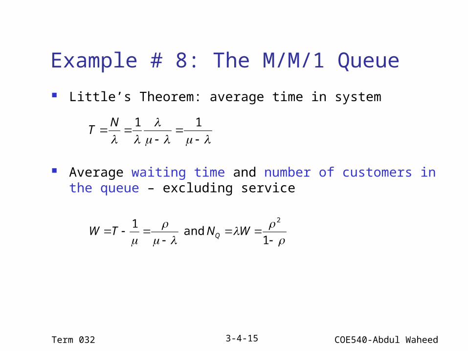
Example # 8: The M/M/1 Queue

Little’s Theorem: average time in system

Average waiting time and number of customers in the queue – excluding service

11NT

1 and

1 2

WNTW Q

Documents

Little’s Theorem Examples Courtesy of: Dr. Abdul Waheed (previous instructor at COE)