Embed Size (px)
Citation preview

Co-published by
Influent Constituent Characteristics of theModern Waste Stream from Single Sources:
Literature Review
Wastewater Treatment and Reuse
04-DEC-1a.qxd 3/2/07 12:50 PM Page 1 (2,1)

04-DEC-1a
INFLUENT CONSTITUENT CHARACTERISTICS OF THE MODERN
WASTE STREAM FROM SINGLE SOURCES: LITERATURE REVIEW
by: Kathryn S. Lowe Nathan K. Rothe Jill M.B. Tomaras Kathleen DeJong Maria B. Tucholke Dr. Jörg Drewes
Dr. John E. McCray Dr. Junko Munakata-Marr Colorado School of Mines
Environmental Science and Engineering Division
2007
Influent Constituent Characteristics of the Modern Waste Stream from Single Sources i

The Water Environment Research Foundation, a not-for-profit organization, funds and manages water quality research for its subscribers through a diverse public-private partnership between municipal utilities, corporations, academia, industry, and the federal government. WERF subscribers include municipal and regional water and wastewater utilities, industrial corporations, environmental engineering firms, and others that share a commitment to cost-effective water quality solutions. WERF is dedicated to advancing science and technology addressing water quality issues as they impact water resources, the atmosphere, the lands, and quality of life. For more information, contact: Water Environment Research Foundation 635 Slaters Lane, Suite 300 Alexandria, VA 22314-1177 Tel: (703) 684-2470 Fax: (703) 299-0742 www.werf.org [email protected] This report was co-published by the following organization. For non-subscriber sales information, contact: IWA Publishing Alliance House, 12 Caxton Street London SW1H 0QS, United Kingdom Tel: +44 (0) 20 7654 5500 Fax: +44 (0) 20 7654 5555 www.iwapublishing.com [email protected] © Copyright 2007 by the Water Environment Research Foundation. All rights reserved. Permission to copy must be obtained from the Water Environment Research Foundation. Library of Congress Catalog Card Number: 2006930842 Printed in the United States of America IWAP ISBN: 1-84339-773-0 This report was prepared by the organization(s) named below as an account of work sponsored by the Water Environment Research Foundation (WERF). Neither WERF, members of WERF, the organization(s) named below, nor any person acting on their behalf: (a) makes any warranty, express or implied, with respect to the use of any information, apparatus, method, or process disclosed in this report or that such use may not infringe on privately owned rights; or (b) assumes any liabilities with respect to the use of, or for damages resulting from the use of, any information, apparatus, method, or process disclosed in this report. Colorado School of Mines The research on which this report is based was developed, in part, by the United States Environmental Protection Agency (EPA) through Cooperative Agreement No. X-830851 with the Water Environment Research Foundation (WERF). However, the views expressed in this document are solely those of Colorado School of Mines and neither EPA nor WERF endorses any products or commercial services mentioned in this publication. This report is a publication of WERF, not EPA. Funds awarded under the Cooperative Agreement cited above were not used for editorial services, reproduction, printing, or distribution. This document was reviewed by a panel of independent experts selected by WERF. Mention of trade names or commercial products does not constitute WERF nor EPA endorsement or recommendations for use. Similarly, omission of products or trade names indicates nothing concerning WERF's or EPA's positions regarding product effectiveness or applicability.
ii

This research was funded by the Water Environment Research Foundation.
ACKNOWLEDGMENTS
Report Preparation Principal Investigator: Kathryn S. Lowe Colorado School of Mines
Co-Principal Investigators: Jörg Drewes, Ph.D. John E. McCray, Ph.D. Junko Munakata-Marr, Ph.D. Colorado School of Mines
Project Team: Kathleen DeJong Nathan K. Rothe Jill M. B. Tomaras Maria B. Tucholke Colorado School of Mines
Project Subcommittee Damann Anderson, P.E. Hazen and Sawyer Matt Byers, Ph.D. Zoeller Company Edward Clerico, P.E. American Water Bob Freeman, P.E. U.S. Environmental Protection Agency Anish Jantrania, Ph.D. Virginia Department of Health Charles McEntyre, P.E. Tennessee Valley Authority
Influent Constituent Characteristics of the Modern Waste Stream from Single Sources iii
Barbara Rich Deschutes County Environmental Health Division
Water Environment Research Foundation Staff Director of Research: Daniel M. Woltering, Ph.D. Program Manager: Christine Handog
iv

ABSTRACT AND BENEFITS Abstract:
A literature review was conducted to assess the current status of knowledge on the composition of raw wastewater and primary treated effluent (i.e., septic tank effluent) from single-source onsite wastewater systems. The overall goal of this research project is to characterize the extent of conventional constituents, microbial constituents, and organic wastewater contaminants in single-source onsite raw wastewater and primary treated effluent to aid onsite wastewater system design and management. Information obtained was evaluated using cumulative frequency distributions to compare individual constituent concentrations in various waste streams and by using data qualifiers to enable assessment of parameters that might affect single-source waste stream composition. To supplement information on the single-source raw wastewater and primary treated effluent composition, state agencies responsible for onsite wastewater regulation were contacted to assess the prevalence of different system types installed and in operation. Selected demographics that capture differences in lifestyle habits that could affect raw wastewater composition were also assessed. A large amount of data was captured by this literature review, however information gaps were identified. The information presented here will be used to guide future project monitoring and assessment of modern raw wastewater waste streams.
Benefits:
♦ Compiles and summarizes approximately 150 literature sources from the last 35 years providing numerous individual raw wastewater and primary treated effluent constituent values from a variety of waste sources.
♦ Provides information on raw wastewater and primary treated effluent composition for single sources including: single family residential, multiple family residential, restaurants, schools, offices, rest areas, correctional facilities, nursing homes, a veterinary clinic, and a RV dump.
♦ Presents cumulative frequency distributions to enable the user to assess wastewater constituent concentrations and mass loadings to a treatment unit or the environment.
♦ Describes the prevalence of onsite wastewater system types and utilization across the U.S. and regionally within the U.S.
♦ Identifies gaps in the current knowledge of raw wastewater and primary treated effluent composition from single sources.
Keywords: Onsite wastewater design, onsite wastewater treatment, raw wastewater, single sources.
Influent Constituent Characteristics of the Modern Waste Stream from Single Sources v

TABLE OF CONTENTS
Acknowledgments.......................................................................................................................... iii Abstract and Benefits.......................................................................................................................v List of Tables ............................................................................................................................... viii List of Figures ................................................................................................................................ xi List of Acronyms ......................................................................................................................... xiii Executive Summary ...................................................................................................................ES-1 1.0 Introduction.................................................................................................................... 1-1 1.1 Background and Motivation ................................................................................ 1-1 1.2 Project Objectives ................................................................................................ 1-2 1.3 Project Approach ................................................................................................. 1-2 1.4 Report Organization............................................................................................. 1-3 2.0 OWS Prevalence............................................................................................................. 2-1 2.1 Introduction.......................................................................................................... 2-1 2.2 Methods................................................................................................................ 2-1 2.3 Results .................................................................................................................. 2-4 2.3.1 State and County Prevalence Data........................................................... 2-4 2.3.2 Census Information................................................................................ 2-11 2.4 Discussion.......................................................................................................... 2-22 3.0 Single-Source Composition ........................................................................................... 3-1 3.1 Introduction.......................................................................................................... 3-1 3.2 Methods................................................................................................................ 3-2 3.3 Results .................................................................................................................. 3-6 3.3.1 Tier 1: Conventional Constituents .......................................................... 3-6 3.3.2 Tier 2: Oil and Grease and Microbial Constituents .............................. 3-24 3.3.3 Tier 3: Trace Organic Wastewater Constituents................................... 3-32 3.4 Discussion.......................................................................................................... 3-37 3.4.1 Data Qualifiers ....................................................................................... 3-39 3.4.2 Waste Stream Variations........................................................................ 3-42 3.4.3 Constituent Comparison......................................................................... 3-54 3.4.4 Informational Gaps ................................................................................ 3-56 4.0 Summary and Conclusions............................................................................................ 4-1 Appendix A: American Housing Survey Methods .................................................................... A-1 Appendix B: State and County Database Listings......................................................................B-1 Appendix C: Complete Listing of Reported BOD Values..........................................................C-1 Appendix D: Complete Listing of Reported Solids Values....................................................... D-1 Appendix E: Complete Listing of Reported Nutrient (Nitrogen and Phosphorus) Values.........E-1 Appendix F: Complete Listing of Reported Fecal Coliform Values ..........................................F-1 Appendix G: Complete Listing of Reported Flow Values......................................................... G-1
vi

Appendix H: Complete Listing of Reported Oil and Grease Values......................................... H-1 Appendix I: Complete Listing of Other Reported Values ...........................................................I-1 References....................................................................................................................................R-1 R.1 Report References................................................................................................R-1 R.2 Data References ...................................................................................................R-8
Influent Constituent Characteristics of the Modern Waste Stream from Single Sources vii

LIST OF TABLES 2-1 Poverty Thresholds as Listed by the U.S. Census Bureau............................................... 2-4 2-2 Summary of Florida OWS ............................................................................................... 2-5 2-3 Summary of Representative New Mexico OWS ............................................................. 2-6 2-4 Summary of Representative North Carolina Large Flow (>3,000 gpd) OWS ................ 2-8 2-5 Summary of Boulder County, Colorado OWS ................................................................ 2-9 2-6 Summary of Single-Source OWS Prevalence for Available State Databases ............... 2-10 2-7 Summary of Percent Occurrence of Single Sources Served by OWS ........................... 2-11 2-8 Total Housing Units....................................................................................................... 2-12 2-9 Occupied Housing Units Served by OWS, Compiled from AHS (2001)...................... 2-13 2-10 Characteristics of U.S. OWS ......................................................................................... 2-16 2-11 AHS Data for Total and New Construction of Occupied Housing Units ...................... 2-20 3-1 Descriptive Statistics for Raw Wastewater and STE BOD5 by Source (in mg/L)........... 3-7 3-2 Descriptive Statistics for Raw Wastewater and STE TSS by Source (in mg/L) ........... 3-10 3-3 Descriptive Statistics for Raw Wastewater and STE Nitrogen by Source (in mg/L) .... 3-15 3-4 Descriptive Statistics for Raw Wastewater and STE Total Phosphorus
by Source (in mg/L) ....................................................................................................... 3-17 3-5 Descriptive Statistics for Raw Wastewater and STE Fecal Coliform
by Source (in cfu/100 Ml).............................................................................................. 3-20 3-6 Descriptive Statistics for Raw Wastewater and STE Flow Rate by Source (in gpd) .... 3-23 3-7 Descriptive Statistics for Raw Wastewater and STE Oil and Grease by
Source (in mg/L) ............................................................................................................ 3-24 3-8 Literature Values for Concentration of Selected Microorganisms found in STE.......... 3-27 3-9 Microorganism Concentration found in Raw Wastewater and STE.............................. 3-27 3-10 Pathogenic Microorganisms found in Raw Wastewater and STE................................. 3-28 3-11 Onsite Wastewater Microbial Research Focus .............................................................. 3-30 3-12 Example of Occurrence (mg/L) of Select Organic Wastewater Contaminants in WWPT Influent and Effluent......................................................................................... 3-33 3-13 Summary of Reported Studies Quantifying the Occurrence of Organic Wastewater Contaminants (OWC) in STE ........................................................................................ 3-36 3-14 Summary of Data Qualifiers for Sorting and Evaluation of Literature Values ............. 3-40 3-15 Median and Normalized Values for Major Constituents by Source .............................. 3-43 3-16 Comparison of Constituent Median Values and Ranges for Single-Source
Domestic Raw Wastewater ............................................................................................ 3-54 3-17 Comparison of Constituent Median Values and Ranges for Single-Source
Domestic STE ................................................................................................................ 3-55 3-18 Summary of the Number of Literature Sources on OWS Raw Wastewater and STE
Composition................................................................................................................... 3-56 A-1 2003 Supplemental Sample Size for Each of the Six AHS-National-Based
Metropolitan Areas ......................................................................................................... A-5 A-2 Interview Activity for Each of the Six 2003 AHS-National-Based
Metropolitan Areas ......................................................................................................... A-6 B-1 Complete List of Florida OWS........................................................................................B-2 B-2 Complete Listing of North Carolina OWS ......................................................................B-4 B-3 American Housing Survey (AHS) Summary of OWS ....................................................B-5
viii

B-4 1990 U.S. Census Information Regarding OWS per State ..............................................B-6 B-5 2000 U.S. Census Information Regarding Over Age 65 by State ...................................B-7 B-6 2000 U.S. Census Information Regarding OWS Location (Rural Vs. Urban)
per State ...........................................................................................................................B-9 B-7 U.S. Census 2004 Poverty Data.....................................................................................B-10 B-8 State Average Annual Precipitation and Temperature...................................................B-12 C-1 Reported Single-Source Domestic BOD5 Raw Wastewater Values................................C-3 C-2 Reported Multiple-Source Domestic BOD5 Raw Wastewater Values ............................C-4 C-3 Reported Food Source BOD5 Raw Wastewater Values ..................................................C-4 C-4 Reported Non-Medical Source BOD5 Raw Wastewater Values .....................................C-5 C-5 Reported Single-Source Domestic BOD5 STE Values....................................................C-5 C-6 Reported Multiple-Source Domestic BOD5 STE Values ................................................C-9 C-7 Reported Food Source BOD5 STE Values.....................................................................C-10 C-8 Reported Non-Medical Source BOD5 STE Values .......................................................C-11 C-9 Reported Medical Source BOD5 STE Values................................................................C-15 C-10 Reported Municipal Source BOD5 Raw Wastewater and STE Values .........................C-16 C-11 Other Reported Oxygen Demand Values ......................................................................C-17 C-12 Other Reported Carbon Values......................................................................................C-21 D-1 Reported Single-Source Domestic TSS Raw Wastewater Values.................................. D-3 D-2 Reported Multiple-Source Domestic TSS Raw Wastewater Values .............................. D-4 D-3 Reported Food Source TSS Raw Wastewater Values .................................................... D-4 D-4 Reported Non-Medical Source TSS Raw Wastewater Values ....................................... D-5 D-5 Reported Single-Source Domestic TSS STE Values...................................................... D-5 D-6 Reported Multiple-Source Domestic TSS STE Values .................................................. D-9 D-7 Reported Food Source TSS STE Values ........................................................................ D-9 D-8 Reported Non-Medical Source TSS STE Values ......................................................... D-11 D-9 Reported Medical Source TSS STE Values.................................................................. D-14 D-10 Reported Municipal Source TSS Raw Wastewater and STE Values ........................... D-15 D-11 Other Reported Solids Values....................................................................................... D-16 E-1 Reported Single-Source Domestic Nitrogen Raw Wastewater Values ...........................E-3 E-2 Reported Multiple-Source Domestic Nitrogen Raw Wastewater Values........................E-4 E-3 Reported Multiple-Source Domestic Nitrogen Raw Wastewater Values........................E-5 E-4 Reported Single-Source Domestic Nitrogen STE Values ...............................................E-5 E-5 Reported Multiple-Source Domestic Nitrogen STE Values..........................................E-13 E-6 Reported Food Source Nitrogen STE Values ................................................................E-14 E-7 Reported Non-Medical Source Nitrogen STE Values ...................................................E-14 E-8 Reported Medical Source Nitrogen STE Values ...........................................................E-22 E-9 Reported Municipal Source Nitrogen Raw Wastewater and STE Values.....................E-23 E-10 Other Reported Nitrogen Raw Wastewater and STE Values ........................................E-23 E-11 Reported Single-Source Domestic Total Phosphorus Raw Wastewater Values ...........E-25 E-12 Reported Multiple-Source Domestic Total Phosphorus Raw Wastewater Values........E-25 E-13 Reported Non-Medical Source Total Phosphorus Raw Wastewater Values .................E-26 E-14 Reported Single-Source Domestic Total Phosphorus STE Values................................E-26 E-15 Reported Multiple-Source Domestic Total Phosphorus STE Values ............................E-28 E-16 Reported Food Source Total Phosphorus STE Values ..................................................E-28 E-17 Reported Non-Medical Source Total Phosphorus STE Values .....................................E-29 E-18 Reported Municipal Source Total Phosphorus Raw Wastewater and STE Values .......E-32 E-19 Other Reported Phosphorus Raw Wastewater and STE Values....................................E-33
Influent Constituent Characteristics of the Modern Waste Stream from Single Sources ix

F-1 Reported Single-Source Domestic Fecal Coliform Raw Wastewater Values .................F-3 F-2 Reported Single-Source Domestic Fecal Coliform STE Values .....................................F-3 F-3 Reported Multiple-Source Domestic Fecal Coliform STE Values..................................F-6 F-4 Reported Non-Medical Source Fecal Coliform STE Values...........................................F-6 F-5 Other Reported Microorganism Values ...........................................................................F-8 G-1 Reported Single-Source Domestic Flow STE Values .................................................... G-2 G-2 Reported Multiple-Source Domestic Flow STE Values................................................. G-2 G-3 Reported Food Source Flow STE Values ....................................................................... G-3 G-4 Reported Non-Medical Source Flow STE Values .......................................................... G-3 H-1 Reported Single-Source Domestic Oil and Grease Raw Wastewater Values................. H-2 H-2 Reported Non-Medical Source Oil and Grease Raw Wastewater Values ...................... H-2 H-3 Other Reported Fats/Oil/Grease Raw Wastewater Values ............................................. H-2 H-4 Reported Single-Source Domestic Oil and Grease STE Values..................................... H-2 H-5 Reported Food Source Oil and Grease STE Values ....................................................... H-3 H-6 Reported Non-Medical Source Oil and Grease STE Values .......................................... H-4 I-1 Reported Ph Values...........................................................................................................I-2 I-2 Reported Alkalinity (as CaCo3) Values ............................................................................I-3 I-3 Reported Hardness (as CaCo3) Values .............................................................................I-3 I-4 Reported Temperature (OC) Values ..................................................................................I-4 I-5 Reported Dissolved Oxygen (mg/L) Values.....................................................................I-4 I-6 Reported Turbidity (ntu) Values.......................................................................................I-5 I-7 Reported Anion and Cation (mg/L) Values ......................................................................I-5
x

LIST OF FIGURES
2-1 Summary of Florida Known Non-Residential Single-Source OWS Greater Than 1% Prevalence.................................................................................................................. 2-5 2-2 Summary of Representative New Mexico Known Non-Residential Single-Source
OWS Prevalence .............................................................................................................. 2-6 2-3 Summary of Representative North Carolina Large Flow (>3,000 gpd) Single-Source
OWS Prevalence .............................................................................................................. 2-7 2-4 Summary of Boulder County, Colorado Non-Residential Single-Source
OWS Prevalence .............................................................................................................. 2-9 2-5 Summary of Single-Source OWS Prevalence for Available State Databases ............... 2-10 2-6 Summary of Percent Occurrence of Single-Source Served by OWS ............................ 2-11 2-7 Percentage of all OWS in the U.S., by Region .............................................................. 2-12 2-8 Percentage of Region’s Occupied Households Served by OWS................................... 2-12 2-9 Total Number of Housing Units with OWS in 1990 ..................................................... 2-14 2-10 Percent Total Housing Units Served by OWS............................................................... 2-15 2-11 Percentage of the Region’s Demographic Category Served by OWS........................... 2-16 2-12 Percent of Total Occupied Housing Units per Region Served by OWS Where
Householder is Older than 65 Years .............................................................................. 2-17 2-13 Percentage of Total Occupied Housing Units in Rural Areas, by Region..................... 2-18 2-14 Percentage of Total Occupied Housing Units in Rural Areas, by State ........................ 2-18 2-15 Percent of the Population in Poverty per Total Occupied Housing Units ..................... 2-19 2-16 Trends in OWS Based on AHS Data ............................................................................. 2-20 2-17 Average Annual Precipitation per State......................................................................... 2-21 2-18 Average Annual Temperature per State......................................................................... 2-21 3-1 Raw Wastewater BOD5 by Source .................................................................................. 3-8 3-2 STE BOD5 by Source....................................................................................................... 3-8 3-3 Comparison of BOD5 in Single-Source Domestic Raw Wastewater and STE................ 3-9 3-4 Raw Wastewater TSS by Source ................................................................................... 3-12 3-5 STE TSS by Source ....................................................................................................... 3-12 3-6 Comparison of TSS in Single-Source Domestic Raw Wastewater and STE................. 3-13 3-7 Raw Wastewater Total Nitrogen.................................................................................... 3-16 3-8 STE Total Nitrogen by Source....................................................................................... 3-16 3-9 Comparison of Total Phosphorus in Single-Source Domestic Raw Wastewater
and STE.......................................................................................................................... 3-18 3-10 STE Total Phosphorus by Source .................................................................................. 3-19 3-11 Comparison of Fecal Coliform in Single-Source Domestic Raw Wastewater
and STE.......................................................................................................................... 3-20 3-12 STE Fecal Coliform by Source ...................................................................................... 3-21 3-13 STE Flow Rate by Source.............................................................................................. 3-23 3-14 STE Oil and Grease by Source ...................................................................................... 3-25 3-15 Example of Variability within the Reported Data Illustrated by a CFD........................ 3-38 3-16 Cumulative Normalized Median Values for Constituent by Source ............................. 3-43 3-17 Cumulative Normalized Median Values for Constituent by Region ............................. 3-45 3-18 Single Source Domestic BOD5 by Decade .................................................................... 3-46 3-19 Single-Source Domestic TSS by Decade....................................................................... 3-46
Influent Constituent Characteristics of the Modern Waste Stream from Single Sources xi

3-20 Single-Source Domestic Total Nitrogen by Decade...................................................... 3-47 3-21 Single-Source Domestic Total Phosphorus by Decade ................................................. 3-48 3-22 Cumulative Normalized Interquartile Range Values for Type of Sample..................... 3-50 3-23 Cumulative Normalized Interquartile Range Values for Analytical Methods............... 3-52 3-24 Cumulative Normalized Interquartile Range Values for Sampling Events ................... 3-53
xii

LIST OF ACRONYMS
AHS American Housing Survey BOD biochemical oxygen demand BOD5 biochemical oxygen demand, five-day test CFD cumulative frequency distribution cfu colony forming unit DNA deoxyribonucleic acid HPLC high performance liquid chromatography GC/MS gas chromatography / mass spectrometry LAS linear alkylbenzene sulfonate MPN most probable number NSFC National Small Flows Clearinghouse NOWRA National Onsite Wastewater Recycling Association OWS onsite wastewater systems PAH polycyclic aromatic hydrocarbon PCB polychlorinated biphenyls pfu plaque forming unit RNA ribonucleic acid STE septic tank effluent TSS total suspended solids U.S. United States U.S. EPA United States Environmental Protection Agency VOC volatile organic compound WWTP wastewater treatment plant
Influent Constituent Characteristics of the Modern Waste Stream from Single Sources xiii

xiv

Influent Constituent Characteristics of the Modern Waste Stream from Single Sources
EXECUTIVE SUMMARY
Proper onsite wastewater system (OWS) design, installation, operation, and management are essential to ensure protection of the water quality and the public served by that water source. Ideally, an OWS should perform reliably and achieve the desired risk management goals over a design life that can be 10 to 20 years or more. Conventional OWS rely on septic tanks for the primary digestion of raw wastewater followed by discharge of primary treated effluent (i.e., septic tank effluent) to the subsurface soils for eventual recharge to underlying groundwater. Over the last 35 years, there have been increasing uses of alternative OWS that rely on additional treatment of the primary treated effluent prior to discharge to the environment in sensitive areas or may eliminate use of a septic tank altogether. Waste streams to be treated by OWS have also changed in recent years due to changing lifestyles including increasing use of personal care and home cleaning products, increasing use of pharmaceutically active compounds (e.g., antibiotics), and lower water use due to water conservation efforts. In each case, understanding the raw wastewater composition based on the single-source type is critical for:
♦ successful OWS design,
♦ informed management decisions, and
♦ assessment of OWS performance and environmental impacts.
The overall goal of this research project is to characterize the extent of conventional constituents, microbial constituents, and organic wastewater contaminants in single-source OWS raw wastewater and primary treated effluent to aid OWS system design and management. This report describes the work performed and results to meet the first project objective of determining the current state of knowledge and identification of knowledge gaps in single-source OWS raw wastewater and primary treated effluent composition.
Information obtained from the literature was evaluated using cumulative frequency distributions to compare individual constituent concentrations in various specific waste streams. There was limited information for OWS raw wastewater relative to primary treated effluent values. In addition, domestic sources are generally well characterized compared to the diverse variety of other (non single-family residential) sources.
To provide additional insight into the reported data values, data qualifiers were used to investigate individual parameters that may affect either the expected median value or the variability within a reported data range. Five key conditions were identified: methods, frequency and duration, date of study, geography, and literature source. There was an apparent regional difference in waste stream composition with the largest difference between the Midwest and West. The most notable changes in constituent concentrations over the last 30 years were for total nitrogen and total phosphorus. Total nitrogen concentrations appear to have declined between the 1970s and the 1990s followed by an increase in 2000 to the present. The total phosphorus concentration decreased between the 1970s and the 1990s and has remained relatively low through the present. The study methods were also found to impact the reported data quality. The type of sample (grab and composite) had the largest effect and the analytical methods employed had the lowest apparent effect. Finally, no trend in the reported data was observed based on the literature source, because nearly 90% of all reported literature values were from similar sources.
ES-1

To supplement information on the single-source OWS composition, the prevalence of
various single-source OWS currently installed and in operation were assessed. American Housing Survey data indicates that 21.0% of all occupied households are served by OWS and that 28% of new construction utilizes OWS. Domestic (residential) sources account for a minimum of approximately 75% of OWS within a state with a wide assortment of non-residential sources also identified. Selected demographics that could affect differences in lifestyle habits and ultimately the raw wastewater composition were assessed. There appear to be three distinct regional locations that encompass the observed differences in the characteristics; 1) the South, 2) the Midwest and Northeast, and 3) the West. Several states stand out as representative to capture differences in the OWS prevalence and demographic characteristics. Florida has a medium percentage of the region’s occupied households served by OWS, high annual average temperature and precipitation, low percentage of rural systems, average levels of poverty, and high percentage of individuals over age 65. Maine has a high percentage of the region’s occupied households served by OWS, low annual average temperature, high annual average precipitation, high percentage of rural systems, average levels of poverty, and medium percentage of individuals over age 65. Colorado has a low percentage of the region’s occupied households served by OWS, low annual average temperature and precipitation, low percentage of rural systems, low levels of poverty, and low percentage of individuals over age 65.
While a large amount of data was captured by this literature review, information gaps were identified including:
♦ limited information on the prevalence of OWS types was readily available,
♦ limited raw wastewater data is available,
♦ limited non-domestic raw wastewater and primary treated effluent data is available,
♦ limited studies reported a full suite of comparable constituents (e.g., biochemical oxygen demand + total suspended solids + total nitrogen + total phosphorus + etc.) for each waste stream characterized, and
♦ limited information on the microbial community or trace organic constituents.
The information presented here will be used to guide future project monitoring and assessment of modern raw wastewater streams.
ES-2

Influent Constituent Characteristics of the Modern Waste Stream from Single Sources 1-1
CHAPTER 1.0
INTRODUCTION
1.1 Background and Motivation
Decentralized wastewater management involving onsite wastewater systems (OWS) has been recognized as a necessary and appropriate component of a sustainable wastewater infrastructure (U.S. EPA, 1997, 2002). OWS currently serve over 21% of the U.S. population and about 28% of all new residential development (AHS, 2001). In Colorado alone, there are over 600,000 OWS in operation with 7,000 to 10,000 new systems installed every year, amounting to over 100 billion liters of wastewater processed and discharged to the environment by OWS each year (DeJong et al., 2004).
Proper OWS design, installation, operation, and management are essential to ensure protection of the water quality and the public served by that water source. Ideally, an OWS should perform reliably and achieve the desired risk management goals over a design life that can be 20 years or more. Field evaluations often examine and assess the suitability of a site based on soil permeability, unsaturated zone depth, and setback distances to drinking water wells and surface waters. Assuming soils and site conditions are judged suitable, a wide variety of OWS are designed and implemented (U.S. EPA, 1997, 2002; Crites and Tchobanoglous, 1998; Siegrist, 2001). Conventional OWS rely on septic tanks for the primary digestion of raw wastewater followed by discharge of septic tank effluent (STE) to the subsurface soils for eventual recharge to underlying groundwater (Crites and Tchobanoglous, 1998; Metcalf and Eddy, 1991; U.S. EPA, 2002). However, increasing uses of alternative OWS rely on additional treatment of the STE prior to discharge to the environment in sensitive areas or may eliminate use of a septic tank altogether. In addition, waste streams to be treated by OWS have changed during recent years due to changing lifestyles including increasing use of personal care and home cleaning products and lower water use due to water conservation efforts. In each case, the raw wastewater composition and concentration varies based on the source type (e.g., single-family home, restaurant, etc.) as well as with time (e.g., daily, weekly, etc.). Information on the composition of single-source OWS raw wastewater is critical for:
♦ successful OWS design to achieve desired levels of treatment prior to discharge in the environment,
♦ informed management decisions to ensure protection of public health and the environment, and
♦ use of available tools, such as model simulations at the single site-scale and the watershed-scale, to assess the effect of OWS performance and water quality impact.
While much research has been done to understand the composition of STE and its treatment in the soil or with engineered treatment units, limited information on raw wastewater is available. Data reported are often of different quality or type, limiting the usefulness of the information. Furthermore, scientific understanding has not been fully or clearly documented, with studies and observations published in project reports and other formats not widely available to the field or not published at all, but retained by the researcher or practitioner (Siegrist, 2001).

The work presented here is part of a larger project to assess the influent constituent characteristics of the modern waste stream from single sources. Results from this literature review document the current understanding of single-source OWS raw wastewater composition, identify gaps in this current knowledge, identify the prevalence of different types of single-source OWS types, and will be used to guide future monitoring and assessment of modern raw wastewater waste streams.
1.2 Project Objectives The overall goal of this research project is to characterize the extent of conventional
constituents, microbial constituents, and organic wastewater contaminants in single-source OWS raw wastewater and primary treated effluent (i.e., STE) to aid OWS system design and management. Specific objectives include:
♦ determine the current state of knowledge related to the characteristics of single-source OWS raw wastewater,
♦ assess single-source OWS raw wastewater,
♦ assess variations in single-source OWS raw wastewater composition, and
♦ transfer the findings to the scientific community, system designers, and decision-makers.
In addition to the above objectives related to raw wastewater, the current state of knowledge for STE was also assessed. The composition of the raw wastewater: 1) is expected to be highly variable, 2) may not reflect constituents of interest present, such as some trace organic contaminants which undergo transformation in the septic tank prior to discharge to the environment, and 3) will not reflect treatment achieved in the tanks used in the majority of OWS to equalize flow and provide primary treatment prior to discharge to the environment (soil treatment unit) or for further treatment (engineered pretreatment unit). Results from the work described in this report are also being shared with the companion Water Environment Research Federation project (04-DEC-7) entitled, Primary Treatment in Onsite Systems: Factors That Influence Performance for incorporation into the database under development in the companion project.
This report describes the work performed and results to meet the first objective of determining the current state of knowledge and identification of knowledge gaps in single-source OWS raw wastewater and STE composition. This information will be used to guide future project monitoring and assessment of modern raw wastewater waste streams.
1.3 Project Approach The first step of the overall project was to conduct a literature review to assess the current
status of knowledge of the composition of waste streams from single-source OWS. To ensure results from the literature review were sound, available information was obtained from peer-reviewed journal publications, peer-reviewed conference proceedings (e.g., American Society of Agricultural Engineers [ASAE] now referred to as The American Society of Agricultural and Biological Engineers), less widely distributed publications and project reports, and from solicitations to individual researchers and experts in the OWS field. No attempt was made to screen, weight, or rank the available data. However, within the Excel database, qualifiers were
1-2

Influent Constituent Characteristics of the Modern Waste Stream from Single Sources 1-3
used to enable sorting of the data to evaluate what effect the parameter may or may not have on the single-source waste stream composition. The data were then compiled into summary tables and cumulative frequency distribution (CFD) graphs. Compilation of the data enables review of the data in many ways to help determine key conditions potentially affecting the composition of a single-source waste stream. The database provides assessment of the available data from the individual’s perspective to address specific and potentially unique questions or needs. These compilations and the database provide tools for prediction of waste stream composition useful in OWS design based on the available data. Finally, CFDs also illustrate the amount of available data (or lack of) as shown by the individual data points used to generate the distribution curves. To supplement information on the single-source OWS composition, the frequencies of various single-source OWS currently installed and in operation were assessed.
1.4 Report Organization This report is organized into four chapters. The first chapter provides an introduction and
purpose for this literature review. Chapter 2.0 describes the prevalence of OWS within the United States based on available records. The composition of single-source OWS raw wastewater and primary treated effluent is presented in Chapter 3.0. Chapter 4.0 summarizes the data collected from the literature and provides conclusions and recommendations for future monitoring. Compilation tables of all the reported data found are provided in appendices.

1-4

Influent Constituent Characteristics of the Modern Waste Stream from Single Sources 2-1
CHAPTER 2.0
OWS PREVALENCE 2.1 Introduction
Currently over 60 million people in the United States live in homes served by OWS (Crites and Tchobanoglous, 1998). Based on U.S. Census information this equates to over 20% of occupied households served by OWS (AHS, 2001). Not only do OWS serve residential homes, they also serve public facilities, industrial parks, and commercial establishments. Although numerous studies have examined the composition of residential primary treated effluent (i.e., STE), few have investigated the composition of raw wastewater or STE from non-residential sources. Due to the variety of source activities the composition of non-residential systems varies greatly. For example, waste streams from restaurants have higher levels of biochemical oxygen demand (BOD), fats, oils, and grease. Institutions such as hospitals, schools, and daycare centers are expected to have a higher rate of pathogen occurrence due to the high density of potential carriers of disease, and hospitals also have higher levels of trace organic contaminants. Examining and characterizing the raw wastewater and STE from single sources will aid in OWS design. Based on the source type, it may be determined that some waste streams warrant distinct pretreatments (i.e. removal of solids, nitrogen reduction, phosphorus or pathogen removal) prior to discharge to the environment (e.g., discharge to bodies of water, subsurface soil dispersal, biosolids management). A different issue is ensuring that sufficient replicates of the waste source have been characterized such that insight is gained into the expected or likely variability within a single-source waste stream.
For this report, data regarding single-source prevalence was ultimately categorized as domestic (residential), food, medical, and non-medical sources. Domestic, a somewhat exclusive category, only consists of single-family residential households and small multifamily housing (< 8 units). The food category includes restaurants, delis, and other structures with food preparation as the main function. Medical sources include both human medical practices as well as veterinary clinics. Finally, non-medical includes all other sources (e.g., schools, day care centers, gas stations, mobile home parks, hotel/motels, etc.).
2.2 Methods In order to assess the prevalence of various single-source OWS currently installed,
several approaches were taken, including contacting state agencies as well as querying the U.S. Census. A list of contact names, phone numbers, and email addresses was acquired from the National Small Flows Clearinghouse (NSFC). The list was comprised of various regulating agencies within each state responsible for implementing OWS regulations. After three attempts to contact all states, 32 states were successfully contacted. Based on the responses of each state’s regulating agency, information regarding source type is maintained primarily on a county level. Even at the county level, many of the databases are not electronic, making a manual search prohibitive (>3000 counties in the U.S.). Furthermore, of the responding states, only Florida,

New Mexico, and North Carolina had databases useful for determining the prevalence of systems.
Both Florida and New Mexico have comprehensive OWS databases. Florida’s database (provided by the Florida Department of Health) is quite detailed and encompasses new permits from 1990 to present (approximately 503,000 entries). New Mexico’s database, found on the New Mexico Environment Department Webpage (www.nmenv.state.nm.us), contains over 100,000 permit entries, although it is not broken down in to individual source types. Two counties, with over 3000 entries, were randomly selected and manually examined to determine OWS type. One county, located in southern New Mexico, includes a mix of urban and rural areas, a higher population density and average household income, and an economic base from service providers, retail businesses, and tourism. The second county, located in northeastern New Mexico, was primarily rural. North Carolina also has an extensive database (found on the North Carolina Department of Environment and Natural Resources, On-Site Wastewater Section webpage at www.deh.enr.state.nc.us) of approximately 2,500 systems, but is restricted to “large” systems as defined by North Carolina as over 3,000 gallons per day (gpd). This North Carolina database provided a more detailed overview of the prevalence of non-residential OWS. Finally, to more closely assess the prevalence of OWS within a single county, the database containing over 18,000 OWS entries was obtained from Boulder County, Colorado. Boulder County is expected to be representative of Colorado as the county has a diverse economic base and distribution including both urban and rural areas, industry, agriculture, older established communities, and new developments. While the OWS prevalence within each state and between counties is expected to vary, Florida, North Carolina, New Mexico, and Boulder County are expected to be representative of the U.S. encompassing different geographic locations, climate conditions, OWS densities, and economic bases.
The prevalence information from these sources was gathered and entered into Excel spreadsheets for further examination and interpretation. Several tables were generated illustrating the most prevalent single sources for each data set. Information was then separated into four general categories: domestic, food, non-medical, and medical.
To supplement the individual state information, the U.S. Census Bureau data was gathered. In addition to taking a census of the population every 10 years, the Census Bureau conducts censuses of economic activity and state and local governments every five years. Every year, the Census Bureau conducts more than 100 other surveys, including the American Housing Survey (AHS). The AHS collects data on the Nation's housing, including number and type of housing (e.g., apartments, single-family homes, mobile homes, and vacant housing units), household characteristics (income, housing, and neighborhood quality), housing costs, equipment and fuels, size of housing unit and recent movers. National data are collected in odd numbered years, and data for each of 47 selected Metropolitan Areas are collected about every six years (U.S. Census Bureau, 2001).
For this study, data from the 2001 AHS was utilized. The 2001 national survey is a sample of about 53,600 interviews. In 2003, the weighting procedures were changed by switching independent estimates from 1990 census-based to 2000 census-based in various steps of the weighting. This included retroactively re-weighting the 2001 AHS according to the 2000 census. The weighting procedures used for AHS partially correct for the bias due to nonresponse and housing unit under coverage, but not for within-household under coverage. The procedures assume the housing units missed by the survey are similar to those included, which may not be entirely accurate. Housing unit under coverage varies by age, ethnicity, and race of householder,
2-2

Influent Constituent Characteristics of the Modern Waste Stream from Single Sources 2-3
and type of household (U.S. Census Bureau, 2001). A more detailed discussion of how the numbers were proportionally adjusted is presented in Appendix A.
AHS data was first examined on a regional basis and then by state. Information gathered for occupied housing units included selected demographic data (age and ethnicity) as well as economic status (living above or below the poverty level). Other characteristics including climate (average temperature and precipitation values obtained from the National Climatic Data Center, NCDC) and urbanization were also compared alongside the AHS data. These characteristics were chosen because of their potential for affecting the composition of OWS raw wastewater.
Data were compiled per state whenever available; however, some data could only be obtained per U.S. Census region. In order to remain consistent with information gathered from other sources, the U.S. Census regions are defined as follows:
♦ Midwest: Illinois, Indiana, Iowa, Kansas, Michigan, Minnesota, Missouri, Nebraska, North Dakota, Ohio, South Dakota, and Wisconsin
♦ Northeast: Connecticut, Maine, Massachusetts, New Hampshire, New Jersey, New York, Pennsylvania, Rhode Island, and Vermont
♦ South: Alabama, Arkansas, Delaware, District of Columbia, Florida, Georgia, Kentucky, Louisiana, Maryland, Mississippi, North Carolina, Oklahoma, South Carolina, Tennessee, Texas, Virginia, and West Virginia
♦ West: Alaska, Arizona, California, Colorado, Hawaii, Idaho, Montana, Nevada, New Mexico, Oregon, Utah, Washington, and Wyoming
Excel was used to create a variety of graphs and charts to illustrate the relationships between the number of households utilizing OWS and other characteristics of importance. Maps were created using MapViewerTM, a mapping and spatial analysis tool developed by Golden Software, Inc. MapViewerTM that creates maps by linking data from a worksheet, such as Excel, to areas or points on a designated map.
First, a base map was created showing the U.S. Census regional areas. From this base map, several additional maps were created to depict other characteristics that may be of importance to OWS. The characteristics included the percent of OWS serving households with elderly residents, the percent serving Hispanic, the percent serving African-American (listed in the Census data as “Black”), as well as the percent serving residents living below the poverty level. Additional maps were generated to depict variation in climate across the U.S., which may have an impact on the raw waste stream.
The following U.S. Census Bureau definitions have been used to create consistency between this report and other surveys performed by the U.S. Census Bureau (2001):
♦ Housing Unit: a house, apartment, group of rooms, or single room occupied or intended for occupancy as separate living quarters.
♦ Occupied Housing Unit: a housing unit where at least one person resides as a usual residence (synonymous to household).
♦ Urban/Rural Housing Units: any housing unit in either an urbanized area or an urbanized cluster. An urbanized area consists of densely settled territory (1,000 or more people per square mile) that contains 50,000 or more people. An urban cluster consists of

densely settled territory that has at least 2,500 people but fewer than 50,000 people. Housing units not classified as urban are considered Rural Housing Units.
♦ Total Number of People Below the Poverty Level: the sum of the number of people in poor families and the number of unrelated individuals with incomes below the poverty threshold. A poor family is defined as a family whose total income is less than the threshold for the family’s size and composition. The dollar amounts of the poverty thresholds used in this report are shown in Table 2-1.
♦ Householder: the first household member listed on the questionnaire that is an owner or renter of the sample unit and is aged 18 years or older.
♦ New Construction: any housing unit less than four years of age. Table 2-1. Poverty Thresholds as Listed by the U.S. Census Bureau (in dollars).
Number of children under 18 years of age Size of Household None 1 2 3 4 5 6 7 >8 1 person
65 years and older Under 65 years
8,259 8,959
2 persons 65 years and older Under 65 years
10,409 11,531
11,824 11,869
3 persons 13,470 13,861 13,874 4 persons 17,761 18,052 17,463 17,524 5 persons 21,419 21,731 21,065 20,550 20,236 6 persons 24,632 24,734 24,224 23,736 23,009 22,579 7 persons 28,347 28,524 27,914 27,489 26,696 25,772 24,758 8 persons 31,704 31,984 31,408 30,904 30,188 29,279 28,334 28,093 9 persons or more 38,138 38,322 37,813 37,385 36,682 35,716 34,841 34,625 33,291
2.3 Results 2.3.1 State and County Prevalence Data
After the prevalence information was gathered, assessment of the types and occurrence of different single-source OWS was evaluated. For this report, unknown sources were determined as an unidentified or unable to be interpreted category from the permit information. Each individual state or county database was summarized in tables and graphically with the percentage of OWS serving each category displayed. Because in each case the occurrence of residential systems greatly exceeded all other types of OWS, the percentage of OWS serving each category was determined as the percent of non-residential systems. Additionally, due to the large number of unknown system types, the percentage of each category was also determined as the percent of non-residential after removing unknown numbers from the database (referred to as the percent known non-residential). This helps to illustrate the diversity of sources served by OWS which would be missed when including the residential or unknown sources.
2.3.1.1 Florida The total number of permits issued in Florida for OWS between 1990 and 2006 was 503,464. While the database included some permit entries dating back to 1920, 99.5% of the entries were between 1990 and 2006. Of these permits, residential systems made up 95.4% (480,914) with less than 1% (524) from unknown sources that could not be categorized. The most prevalent
2-4

Influent Constituent Characteristics of the Modern Waste Stream from Single Sources 2-5
single sources other than residential OWS were offices (19.0% of non-residential OWS), mobile homes/RVs (18.0% of non-residential OWS), warehouses (8.5% of non-residential OWS), and churches (6.0% of non-residential OWS) (Table 2-2 and Figure 2-1). A complete listing of the OWS types is presented in Appendix B (Table B-1).
0%
5%
10%
15%
20%
25%
Office
Mobile
Home/R
V
Warehous
e
Church
Store/Shop Poo
l
Garage
Restaura
ntPark
School
Barn
Commercial
Auto R
epair
Misc
Cabin/C
amp
Acces
ory
Factory
Source Type
Perc
ent o
f all
Kno
wn
Non
-Res
iden
tial S
yste
ms
Florida
Figure 2-1. Summary of Florida Known Non-residential Single-Source OWS Greater Than 1% Prevalence.
Table 2-2. Summary of Florida OWS.
Source Type Number of
Systems Percent of
All Systems
Percent of Non-Residential
Systems
Percent of Known Non-Residential
Systems Residential 480,834 95.5% Unknown 524 0.1% 2.3% Office 4,291 0.8% 19.0% 19.5% Mobile Home/RV 4,064 0.8% 18.0% 18.4% Warehouse 1,924 0.4% 8.5% 8.7% Church 1,348 0.3% 6.0% 6.1% Store/Shop 1,260 0.2% 5.6% 5.7% Pool 1,011 0.2% 4.5% 4.6% Garage 878 0.2% 3.9% 4.0% Restaurant 756 0.2% 3.4% 3.4% Park 595 0.1% 2.6% 2.7% Other 5,979 1.2% 26.5% 27.2% Total 503464 Total Non-Residential 22550 Total Known Non-Residential 22026
1 A complete listing of “other” source types is presented in Appendix B.
2.3.1.2 New Mexico The New Mexico database contains over 100,000 entries (from 1973 – present) that are
not categorized in any way. Two counties were randomly selected with over 3,000 entries which

were manually categorized to gain insight into single-source OWS prevalence in New Mexico. Of these 3000 systems, 94.5% (2,855) were associated with residential systems. Unknown sources (55.3%), churches (14.5%), and hardware stores (3.9%) were the most prevalent non-residential source types (Table 2-3 and Figure 2-2).
0%
10%
20%
30%
40%
Church
Hardware
Store
Fire D
eptFarm
MissionArm
y
Office B
ldg
Commerc
ial
Electric
co-op
Day Sch
ool
Ranch
Monas
tery
Waste
MgmtBan
k
Animal
Rescu
e
Printin
g Co
Teleph
one C
o
Retrea
t Cen
ter
Source Type
Perc
ent o
f All
Kno
wn
Non
-Res
iden
tial S
yste
ms
New Mexico
Figure 2-2. Summary of Representative New Mexico Known Non-residential Single-Source OWS Prevalence.
Table 2-3. Summary of Representative New Mexico OWS.
Source Type Number of
Systems Percent of All
Systems
Percent of Non-Residential
Systems
Percent of Known Non-Residential
Systems Residential 2,855 94.0% - - Unknown 99 3.3% 55.3% - Church 26 0.9% 14.5% 32.5% Hardware Store 7 0.2% 3.9% 8.8% Fire Department 6 0.2% 3.4% 7.5% Farm 5 0.2% 2.8% 6.2% Mission 4 0.1% 2.2% 5.0% Army 4 0.1% 2.2% 5.0% Office Building 3 0.1% 1.7% 3.8% Commercial 3 0.1% 1.7% 3.8% Electric co-op 3 0.1% 1.7% 3.8% Day School 3 0.1% 1.7% 3.8% Ranch 3 0.1% 1.7% 3.8% Monastery 2 0.07% 1.1% 2.5% Waste Management 2 0.07% 1.1% 2.5% Bank 2 0.07% 1.1% 2.5% Animal Rescue 2 0.07% 1.1% 2.5% Printing Company 2 0.07% 1.1% 2.5% Telephone Company 2 0.07% 1.1% 2.5% Retreat Center 1 0.03% 0.6% 1.2% Total 3,034 100% 100% 100% Total Non-Residential 179 Total Known Non-Residential 80
2-6

Influent Constituent Characteristics of the Modern Waste Stream from Single Sources 2-7

2.3.1.3 North Carolina
The North Carolina database provided a more detailed overview of the source distribution of large, non-residential OWS. The North Carolina database contains data for 2,669 large flow OWS (defined by North Carolina as >3,000 gpd; data base includes permits from 1982 – present). Of these 2,669 entries, 500 entries were randomly selected, manually examined, and categorized. Because the database entries were not organized by date, source type, or flow, the 500 randomly selected entries were assumed to be a representative of the database entries. Of these large OWS entries, 25.0% (125) serve unknown sources, 15.6% (78) serve schools, and 8.2% (41) serve residential facilities (apartments, cluster systems, townhouses) (Table 2-4 and Figure 2-3). Figure 2-3 suggests a higher percent of OWS in North Carolina are non-residential compared to Florida or New Mexico. However, almost all residential systems have daily flows <3,000 gpd and were not included in the database examined. While a comparison between residential and non-residential systems cannot be made from the North Carolina database, insight into the source distribution of large systems can be gained. A complete listing of the OWS types for the 500 entries examined is presented in Appendix B (Table B-2).
0%
5%
10%
15%
20%
25%
30%
Unknown
School
Residenti
al
Restaura
nt
Condo
Car was
h
Rest Hom
e
Apartm
ent
Mobile
Home Park
Furnitu
re Co
Campgroun
dPark
Golf C
ourse
ChurchMote
lOffic
e
College
Medica
l
Airport
Grocery
Marina
Mill
Conferen
ce C
enterLa
b
Manufac
turing
Research
Cen
ter
Source Type
Perc
ent o
f all
Syst
ems
North Carolina
Figure 2-3. Summary of Representative North Carolina Large Flow (>3,000 gpd) Single-Source OWS Prevalence.
2-8

Influent Constituent Characteristics of the Modern Waste Stream from Single Sources 2-9
Table 2-4. Summary of Representative North Carolina Large Flow (>3,000 gpd) OWS.
Source Type Number of
Systems Percent of All
Systems
Percent of Non-Residential
Systems
Percent of Known Non-Residential
Systems Unknown 125 25.0% 27.2% - School 78 15.6% 17.0% 23.4% Residential 41 8.2% - - Restaurant 29 5.8% 6.3% 8.7% Condo 20 4.0% 4.4% 6.0% Car wash 15 3.0% 3.3% 4.5% Rest Home 15 3.0% 3.3% 4.5% Apartment 13 2.6% 2.8% 3.9% Mobile Home Park 11 2.2% 2.4% 3.3% Furniture Co 10 2.0% 2.2% 3.0% Campground 9 1.8% 2.0% 2.7% Park 9 1.8% 2.0% 2.7% Golf Course 8 1.6% 1.7% 2.4% Church 7 1.4% 1.5% 2.1% Motel 7 1.4% 1.5% 2.1% Office 6 1.2% 1.3% 1.8% College 5 1.0% 1.1% 1.5% Medical 5 1.0% 1.1% 1.5% Airport 4 0.8% 0.9% 1.2% Grocery 4 0.8% 0.9% 1.2% Marina 4 0.8% 0.9% 1.2% Mill 4 0.8% 0.9% 1.2% Conference Center 3 0.6% 0.7% 0.9% Lab 3 0.6% 0.7% 0.9% Manufacturing 3 0.6% 0.7% 0.9% Research Center 3 0.6% 0.7% 0.9% Other1 59 11.8% 12.9% 17.7% Total 500 100.0% 100.0% 100.0% Total Non-Residential 459 Total Known Non-Residential 334
1 A complete listing of “other” source types is presented in Appendix B.
2.3.1.4 Boulder County, Colorado Boulder County, Colorado was selected to more closely assess the prevalence of OWS
within a single county. The Boulder County database contains 18,735 entries (from 1950 – present), of which 17,716 are for residential OWS (94.6%). The most prevalent non-residential single-source OWS are categorized as other (35.0%), commercial (25.2%), and industrial (7.5%) (Table 2-5 and Figure 2-4). Note, this database separates OWS single sources into more general categories than those used by other states.

0%5%
10%15%20%25%30%35%40%
Other
Commerc
ial
Indus
trial
Camp
Office B
uildin
g
Public
Park
Church
Restau
rant
Resort
Hotel/M
otelBarn
Service
Stat
ion
Day S
choo
l
Studio
Garage
Day C
are
Boardi
ng sc
hool
Cabin
Food S
ervice
Stable
Source Type
Perc
ent o
f all
Non
-Res
iden
tial S
yste
ms
Boulder County
Figure 2-4. Summary of Boulder County, Colorado Non-residential Single-Source OWS Prevalence.
Table 2-5. Summary of Boulder County, Colorado OWS.
Source Type Number of Systems Percent of All Systems Percent of Non-
Residential Systems Residential 17,716 94.6% - Other 357 1.9% 35.0% Commercial 257 1.4% 25.2% Industrial 76 0.4% 7.5% Camp 69 0.4% 6.8% Office Building 60 0.3% 5.9% Public Park 34 0.2% 3.3% Church 33 0.2% 3.2% Restaurant 30 0.2% 2.9% Resort 20 0.1% 2.0% Hotel/Motel 16 0.09% 1.6% Barn 15 0.08% 1.5% Service Station 14 0.07% 1.4% Day School 13 0.07% 1.3% Studio 10 0.05% 1.0% Garage 9 0.05% 0.9% Day Care 2 0.01% 0.2% Boarding school 1 0.01% 0.1% Cabin 1 0.01% 0.1% Food Service 1 0.01% 0.1% Stable 1 0.01% 0.1% Total 18,735 100% 100% Total Non-Residential 1,019
2-10

Influent Constituent Characteristics of the Modern Waste Stream from Single Sources 2-11
2.3.1.5 Summary Based on the specific categories of each OWS source database, prevalence is highest for
residential dwellings, followed distantly by commercial and office structures (Table 2-6 and Figure 2-5). The wide variety of different non-residential OWS types made meaningful assessment of the OWS prevalence difficult. While the North Carolina database provided a more detailed overview of the source distribution of large, non-residential OWS, the database entries were further summarized based on expected wastewater characteristics into four categories: domestic, food, non-medical, and medical. Based on the information available, domestic (residential) sources are the most prevalent single sources served by OWS followed by non-medical, food, and medical (Table 2-7 and Figure 2-6). Again it is important to note that the higher percent of non-residential OWS in North Carolina is due to the database examined containing only information on systems with daily flows >3,000 gpd. Because almost all residential systems have daily flows <3,000 gpd a comparison between residential and non-residential systems cannot be made from the North Carolina database. However, insight into the source distribution of large non-residential systems can be gained.
0%
5%
10%
15%
20%
Florida New Mexico North Carolina Boulder County,CO
Perc
ent o
f all
OW
S ResidentialCommercialOfficeChurchPublic ParkRestaurantSchool
95.5% 94.5% 94.6%
(large systems only, >3,000 gpd)
Figure 2-5. Summary of Single-Source OWS Prevalence for Available State Databases.
Table 2-6. Summary of Single-Source OWS Prevalence for Available State Databases (in % of all OWS).
Source Type Florida New Mexico1 North Carolina2 Boulder County, CO Residential 95.5% 94.5% 8.2% 94.6% Commercial - 0.1% - 1.4%3 Office 0.8% 0.1% 1.2% 0.3% Church 0.3% 0.9% 1.4% 0.2% Public Park 0.1% - 1.8% 0.2% Restaurant 0.2% - 5.8% 0.6% School 0.1% 0.1% 15.6% 0.07% - OWS type not listed in permit database 1 Values represent over 3,000 of the 100,000 available entries 2 Values represent 500 of the 3,000 available large flow (defined by North Carolina as >3,000gpd) entries 3 No additional detail is provided for commercial facilities

0%
20%
40%
60%
80%
100%
Domestic Food Non-Medical Medical
Source Category
Perc
ent O
ccur
ence
FloridaNew MexicoNorth CarolinaBoulder County, CO
Figure 2-6. Summary of Percent Occurrence of Single Sources Served by OWS.
Table 2-7. Summary of Percent Occurrence of Single Sources Served by OWS.
Source Category Florida New Mexico1 North Carolina2 Boulder County,
CO Domestic 95.4% 92.6% 20.0% 94.6% Food 0.2% 0.0% 6.0% 0.2% Non-Medical 4.2% 7.4% 73.0% 5.3% Medical 0.08% 0.0% 1.0% 0.0% 1 Values represent over 3,000 of the 100,000 available entries 2 Values represent 500 of the 3,000 available large flow (defined by North Carolina as >3,000 gpd) entries
2.3.2 Census Information 2.3.2.1 Total Housing Units
According to the 2000 U.S. Census Bureau data, the total number of housing units in the U.S. was 115,904,641. Out of those, 91.0% are considered occupied housing units (Table 2-8). Of all occupied housing units in the U.S., 19.3% are located in the Northeast, 23.2% in the Midwest, 36.0% in the South, and 21.5% in the West. Examination of census data for the AHS (2001) indicated that 21.0% (22,194,000) of all occupied households are served by OWS. This is a slightly lower than the 25% often reported. Because the U.S. Census Bureau relies on the survey response from a limited number of homes and then extrapolates these findings to estimate the reported census data, the difference (4%) may be due to the uncertainty in the U.S. Census Bureau data. If the estimated occupancy per household ranges between 2.5 and 3 persons, approximately 56 to 66 million persons are served by OWS. The U.S. Census Bureau reported an average household size of 2.63 in 1990, 2.59 in 2000, and 2.6 in 2004.
Regionally 19.4% of all OWS are in the Northeast, 22.0% are in the Midwest, 45.3% are in the South, and 13.3% are in the West (Table 2-9 and Figure 2-7). The South has almost half of all OWS in the U.S., more OWS than the Midwest and Northeast combined, and almost three and one half times as many systems as the entire Western region. The national distribution of OWS per U.S. Census region is illustrated in Figure 2.7 (Table 2-9). To assess the amount of OWS within each region, the percent of total occupied households was determined. In the
2-12

Influent Constituent Characteristics of the Modern Waste Stream from Single Sources 2-13
Northeast 21.3% of occupied households are served by OWS, in the Midwest 19.9%, in the South 26.5%, and in the West 13.0% of the occupied households are served by OWS (Table 2-9, Figure 2-8).
Table 2-8. Total Housing Units (AHS, 2001).
Type of Unit Number of Units Total Occupied Housing Units 105,435,000 Total Vacant/Seasonal Units 12,761,000 Total Housing Units 118,196,000
13%
22%19%
46%
Figure 2-7. Percentage of All OWS in the U.S., by Region (AHS, 2001).
13%
20%21%
26%
Figure 2-8. Percentage of Region’s Occupied Households Served by OWS (AHS, 2001).

Table 2-9. Occupied Housing Units Served by OWS, Compiled from AHS (2001).
Region Household Characteristics
United States Northeast Midwest South West
Total Occupied Housing Units in Category 105,435,000 20,352,000 24,446,000 37,976,000 22,662,000
Number of Households Served by OWS 22,194,000 4,311,000 4,874,000 10,061,000 2,948,000
Percentage of All OWS in U.S. 100.0% 19.4% 22.0% 45.3% 13.3%
Percentage of Regional Households Served by OWS 21.0% 21.2% 19.9% 26.5% 13.0%
Total Housing Units Occupied by African-Americans 13,223,000 2,391,000 2,471,000 7,162,000 1,199,000
Number of African-American Households Served by OWS 1,197,000 45,000 44,000 1,092,000 16,000
Percent of Region’s OWS Serving African-American Households
5.4% 1.0% 0. 0% 10.8% 0.5%
Percent of Region’s African-American Households Served by OWS
9.0% 1.9% 1.8% 15.2% 1.3%
Total Housing Units Occupied by Hispanics 9,720,000 1,490,000 739,000 3,596,000 3,895,000
Number of Hispanic Households Served by OWS 696,000 75,000 52,000 306,000 263,000
Percent of Region’s OWS Serving Hispanic Households 3.1% 1.7% 1.1% 3.0% 8.9%
Percent of Region’s Hispanic Households Served by OWS 7.2% 5.0% 7.0% 8.5% 6.8%
Total Housing Units Occupied by Householders Over Age 65 21,656,000 4,785,000 5,098,000 7,786,000 3,987,000
Number of Households Over Age 65 Served by OWS 4,970,000 930,000 987,000 2,391,000 662,000
Percent of Region’s OWS Serving Households Over Age 65
22.4% 21.6% 20.2% 23.8% 22.5%
Percentage of Region’s Households Over Age 65 Served by OWS
23.0% 19.4% 19.4% 30.7% 16.6%
2-14

Influent Constituent Characteristics of the Modern Waste Stream from Single Sources 2-15
Information regarding number of OWS per state is currently available only for the year 1990. The distribution of OWS per state using this data is illustrated in Figure 2-9. Five states (Texas, Florida, North Carolina, Pennsylvania, and New York) had more than 1.2 million OWS, and 28 of the states had less than 400,000 systems. Florida alone had more systems than the entire West region minus California and Washington. On the other hand, eight states had less than 100,000 systems; five of those were in the West region. Interestingly, Washington DC was listed as having 575 systems (approximately 0.2% of the households served by OWS) and 1433 households served by other means (approximately 0.5% of the households served by other means). Other means is defined by the AHS as some means other than public sewer, septic tank, or cesspool. This is an unexpected result and may be attributed to the uncertainty within the survey (e.g., inaccurate survey responses or error due to survey weighting factors). A complete listing of the OWS distribution per state is presented in Appendix B (Table B-4).
Total Number of Housing Units with OWS(US Census 1990)
0 to 400,000400,000 to 800,000800,000 to 1,200,0001,200,000 to 1,600,000
Figure 2-9. Total Number of Housing Units with OWS in 1990 (does not reflect occupied housing units).
It is also interesting to note subtle trends within each region (see Appendix B, Table B-4). For example, Figure 2-10 shows seven states in the South with between 15 and 30% of the housing units served by OWS. Of these seven states, only Maryland and Texas have less than 20% of their housing units served by OWS (Table B-4). Although the South has more systems than any region, North Carolina is the only state in the South where more than 45% of all housing units are served by OWS. Conversely, in the Northeast three states (New Hampshire, Vermont, and Maine) all have more than 45% of their housing units served by OWS (Figure 2-10). This suggests that while the greatest number of OWS is located in the South, portions of the Northeast have a higher percentage of the region’s occupied households served by OWS.

Percent OWS per Total Housing Units(Census 1990)
0 to 1515 to 3030 to 4545 to 60
Figure 2-10. Percent Total Housing Units Served by OWS (circled states have >45% total housing units served by OWS) (U.S. Census, 1990).
2.3.2.2 Demographics Additional information gained from the U.S. Census Bureau (2000) included insight into
the demographics of households being served by OWS. Several specific demographics (i.e. age, location [urban vs. rural], income, and ethnicity) were examined that may affect the wastewater composition due to potential differences in lifestyle habits. Households with occupants over the age of 65 were assessed as these households may be more likely to contribute higher loads of pharmaceuticals and other trace organic wastewater contaminants to the waste stream due to increased use of medications. In addition, households with occupants over the age of 65 were assumed to have fewer total occupants per household resulting in potentially lower water use. The location (urban vs. rural) was assessed due to potential differences in water use. Similar to the location of the household served by OWS, the age of the household with an OWS was summarized because it was assumed newer households would be more likely to have low flow fixtures resulting in lower daily water use. Specific data related to the year of OWS construction was not available in the AHS data; however information related to new construction was collected. Although income (household income above or below the poverty level) and ethnicity may result in different lifestyle habits, it is summarized for informational purposes only. Summaries of the demographic characteristics can be found in Tables 2-9 and 2-10, and Figure 2-11.
2-16

Influent Constituent Characteristics of the Modern Waste Stream from Single Sources 2-17
Table 2-10. Characteristics of U.S. OWS (AHS, 2001).
Category
Total Occupied Housing Units in
Category
Number of Total Occupied Housing
Units Served by OWS
Percentage of All OWS in U.S.
Percentage of Category Total
Occupied Housing Units Served by
OWS Occupied Housing Units in the United States 105,435,000 22,194,000 100.0% 21.0%Urban Households 78,482,000 4,504,000 20.3% 5.7%Rural Households 26,953,000 17,691,000 79.7% 65.6%New Construction Households 5,853,000 1,656,000 7.5% 28.3%Households Below Poverty Level 14,495,000 2,672,000 12.0% 18.4%African-American Households 13,223,000 1,197,000 5.4% 9.0%White Households 82,492,000 20,301,000 91.5% 24.6%Hispanic Households 9,720,000 696,000 3.1% 7.2%Households Under Age 65 83,780,000 17,224,000 77.6% 20.6%Households Over Age 65 21,655,000 4,970,000 22.4% 23.0%
0%
5%
10%
15%
20%
25%
30%
UnitedStates
Northeast Midwest South West
Region
Perc
enta
ge o
f tho
se S
erve
d by
OW
S Total OccupiedElderly (>65)PovertyAfrican-AmericanHispanic
Figure 2-11. Percentage of the Region’s Demographic Category Served by OWS (regional poverty OWS values are unavailable) (AHS, 2001).

Over age 65 Information on the age of the occupants (over 65) was assessed due to
potential differences in waste stream composition based on lower water use and higher trace organic wastewater contaminant loads. Of all the OWS in the U.S., 77.6% (17,224,000) serve the population under age 65 and 22.4% (4,970,000) serve the population over age 65 (Tables 2-9 and 2-10, Figure 2-11). For the over age 65 households, 23.0% are served by OWS which is similar to the distribution of total households served by OWS across the U.S. of 21.0%. This suggests that households with occupants over the age of 65 are no more likely to utilize OWS than the entire U. S. population. However, there are some regional differences. In the South, 23.8% of the total OWS serve households with occupants over the age of 65, but 30.7% percent of the householders over the age of 65 are served by OWS (Figure 2-12). Conversely, in the West, 22.5% of the total OWS serve households with occupants over the age of 65, but only 16.6% of households over age 65 are served by OWS. In other words, households over the age of 65 are more likely to be served by OWS in the South and less likely to be served by OWS in the West compared to households under the age of 65. A complete listing of over age 65, by state, is presented in Appendix B (Table B-5).
17%
20%20%
31%
Figure 2-12. Percent of Total Occupied Housing Units per Region Served by OWS Where Householder is Older than 65 Years (AHS, 2001).
Location Information on the location and OWS age were assessed due to potential differences in waste stream composition based on water use. According to the AHS, approximately 25.6% of all occupied housing units (105,435,000 total households) are rural households (26,953,000), and of these rural households 65.6% of those are served by OWS. Of the remaining 74.4% of occupied urban housing units, only 5.7% of these urban households are served by OWS (Table 2-10). Alternatively, specific to the households in the U.S. utilizing OWS, 79.7% are located in rural locations and 20.3% are located in urban locations.
Similar to total household trends and the age of the householder (over 65), regional differences were observed. The South has the most rural households per region and the West has the fewest (Figure 2-13). More detailed information regarding the percentage of households found in rural areas for individual states is shown in Figure 2-14. In Arkansas, Mississippi, South
2-18

Influent Constituent Characteristics of the Modern Waste Stream from Single Sources 2-19
Dakota, and West Virginia more than 45% of the total occupied units are rural households. In Vermont and Maine, more than 55% of all households are rural. The complete data are provided in Appendix B (Table B-6).
Although the year of construction was not available, the U.S. Census also contained information regarding new construction (defined as households less than four years old). In 2001, 7.5% (1,656,000) of the households in the U.S. utilizing OWS, serve new construction (Table 2-10). Of the new construction, 28.3% is served by OWS which is slightly higher than the distribution across the U.S. of total households served by OWS of 21.0%. This suggests that new construction is more likely to utilize OWS than the entire U.S. population.
12%
15%
25%
27%
Figure 2-13. Percentage of Total Occupied Housing Units in Rural Areas, by Region (U.S. Census, 2000).
Percent Rural Householdsper Total Occupied Units
0 to 1515 to 3030 to 4545 to 61
Figure 2.14. Percentage of Total Occupied Housing Units in Rural Areas, by State (circle indicates state with the highest percentage of rural households) (U.S. Census, 2000).

Poverty and Ethnicity Although income (above or below the poverty level) and ethnicity may result in different lifestyle habits, it is summarized for informational purposes only. Approximately 12.0% (2,672,000) of the total number of OWS in the U.S. serve households below the poverty level (Table 2-10 and Figure 2-11). Of all U.S. households living below poverty level, 18.4% are served by OWS. Data regarding households below the poverty level served by OWS were not available on a regional basis. However, individual state data was available detailing the percent of occupied housing units below the poverty level (U.S. Census 2004). For example, the South has more households living in poverty than any other region (Figure 2-15). More than one fifth of all the population in Mississippi lives in poverty, and almost 40% of all the housing units there are served by OWS. A complete listing of households below the poverty level, by state, is presented in Appendix B (Table B-7).
Of all OWS, 91.5% (20,301,000) serve the white population, 5.4% (1,197,000) serve the African-American population, and 3.1% (696,000) serve the Hispanic population (Tables 2-9 and 2-10, Figure 2-11).
Population living in poverty(%)
0 to 1010 to 1515 to 2020 to 25
Figure 2-15. Percent of the Population in Poverty per Total Occupied Housing Units (circle indicates state with the highest percentage of the population in poverty) (U.S. Census, 2004).
2.3.2.3 Trends in Time
Over the last 35 years, the percentage of households utilizing OWS nationwide appears to have decreased slightly (Figure 2-16 and Table 2-11). Based on the AHS data, a high of 28.4% of the total households were served by OWS in 1973, and a low of 20.5% in 2003. A similar decrease since 1999 was also seen regionally (Appendix B). Not surprisingly, the number of total occupied households has increased. However, the number of total households served by OWS has not increased at a similar rate. Comparison of the new construction of housing units (defined as less than four years old) suggests that the total number of new housing units and the percent of this new construction that utilize OWS have remained relatively constant. The new construction housing units utilizing OWS ranged between 1.4 – 2.4 million units annually between 1973 and
2-20
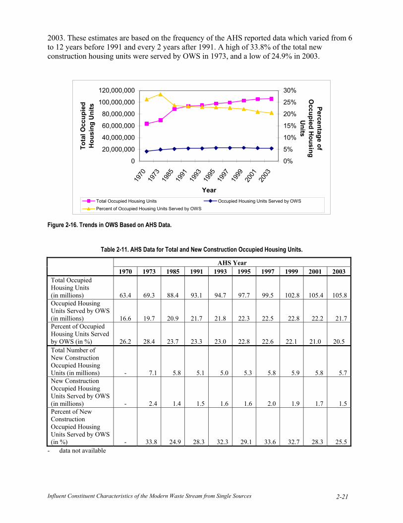
Influent Constituent Characteristics of the Modern Waste Stream from Single Sources 2-21
2003. These estimates are based on the frequency of the AHS reported data which varied from 6 to 12 years before 1991 and every 2 years after 1991. A high of 33.8% of the total new construction housing units were served by OWS in 1973, and a low of 24.9% in 2003.
0
20,000,000
40,000,000
60,000,000
80,000,000
100,000,000
120,000,000
1970
1973
1985
1991
1993
1995
1997
1999
2001
2003
Year
Tota
l Occ
upie
d H
ousi
ng U
nits
0%
5%
10%
15%
20%
25%
30%Percentage of
Occupied H
ousing U
nits
Total Occupied Housing Units Occupied Housing Units Served by OWSPercent of Occupied Housing Units Served by OWS
Figure 2-16. Trends in OWS Based on AHS Data.
Table 2-11. AHS Data for Total and New Construction Occupied Housing Units.
AHS Year 1970 1973 1985 1991 1993 1995 1997 1999 2001 2003
Total Occupied Housing Units (in millions) 63.4 69.3 88.4 93.1 94.7 97.7 99.5 102.8 105.4 105.8 Occupied Housing Units Served by OWS (in millions) 16.6 19.7 20.9 21.7 21.8 22.3 22.5 22.8 22.2 21.7 Percent of Occupied Housing Units Served by OWS (in %) 26.2 28.4 23.7 23.3 23.0 22.8 22.6 22.1 21.0 20.5 Total Number of New Construction Occupied Housing Units (in millions) - 7.1 5.8 5.1 5.0 5.3 5.8 5.9 5.8 5.7 New Construction Occupied Housing Units Served by OWS (in millions) - 2.4 1.4 1.5 1.6 1.6 2.0 1.9 1.7 1.5 Percent of New Construction Occupied Housing Units Served by OWS (in %) - 33.8 24.9 28.3 32.3 29.1 33.6 32.7 28.3 25.5
- data not available

2.3.2.4 Climate
Mapping the average yearly temperature as well as the average yearly precipitation for each state shows distinct climate difference between regions. While not expected to be critical to constituent transformations in the raw wastewater, climate may play an important role in the composition of the primary and secondary treated waste stream due to seasonal variations. For example, extended cool temperatures may inhibit nitrification in soil during the winter season in cold climates (Converse, 1999). Figures 2-17 and 2-18 illustrate the wide range of average annual precipitation and average annual temperature found across the United States (see Appendix B for a complete listing, Table B-8).
Average Annual Precipitation(Inches)
0 to 1515 to 3030 to 4545 to 6060 to 75
Figure 2-17. Average Annual Precipitation per State.
Average Annual TemperatureDegrees Fahrenheit
30 to 4040 to 5050 to 6060 to 7070 to 80
Figure 2-18. Average Annual Temperature per State.
2-22

Influent Constituent Characteristics of the Modern Waste Stream from Single Sources 2-23
2.4 Discussion Based on the results obtained from the available state and county databases, domestic
(residential) sources are the most prevalent (Table 2-7 and Figure 2-6). This is not surprising and is reinforced by the lack of available data regarding STE composition from other sources (Section 3). North Carolina has a higher percentage of non-medical sources probably due to the fact that these systems serve higher flow institutions and were therefore captured by the specific North Caroline database (>3,000 gpd systems only). By summarizing the available data into four categories, comparisons across the databases were made easier; an obvious trend in prevalence was seen for the three databases specific to small flow systems (Florida, New Mexico, and Boulder County, CO) with domestic >> non-medical > food > medical. However, the detailed characteristics within these four categories demonstrate the diverse assortment of institutions utilizing OWS.
Detailed information on the prevalence of OWS types was not obtained. Only Florida, New Mexico, and North Carolina had electronically available databases useful for assessing the prevalence of OWS for this study. In the absence of specific State data, AHS data was used. Because the U.S. Census Bureau survey relies on the response of a subset of the population and then assumes that the results are representative of the entire U.S., there are inherent uncertainties in the estimates. For example, the estimated number of OWS in Florida in 1990 was 1,559,113 (AHS, 1990). However 2,019,106 installations are shown with the permit database obtained from the Florida website (www.doh.state.fl.us/environment/sdtds/statistics/newinstallations.htm). This represents a 22% difference in the AHS estimates compared to the actual numbers maintained by the State. It should be noted that the Florida permit database includes repairs and does not reflect systems that have since been placed on centralized sewers or have been otherwise removed from service while the AHS does not provide information on the type of OWS. While not surprising, this example illustrates the level of detail and type of information that is “lost” when accessible databases are not maintained and the variability in prevalence estimates from different sources.
OWS permit databases are typically kept at the County level providing detailed information to the required regulatory decision makers. Resource limitations (staffing and funding) at the County level may preclude establishing an electronic database with records kept as hard copy files and/or microfiche. In these cases, detail information cannot be readily rolled-up to provide insight within a specific county, state and/or across the U.S. This limited availability of accurate OWS prevalence and type data was identified as an information gap.
Selected demographics were assessed due to differences in lifestyle habits that could affect raw wastewater composition including:
♦ over the age of 65, ♦ location (urban vs. rural), ♦ new construction, and ♦ poverty and ethnicity.
Households with occupants over the age of 65 may be more likely to contribute higher loads of pharmaceuticals and other trace organic wastewater contaminants to the waste stream due to increased use of medications. There may be a difference in water use between rural and urban locations that may affect the wastewater strength. Newly constructed homes may also have lower water use relative to older households due to installation of low flow water fixtures. Although income (household income above or below the poverty level) and ethnicity may result in different lifestyle habits, it was assessed for informational purposes only.

Several characteristics are apparent when examining the 2001 AHS data (Table 2-9). The
South, for example, has the majority of the total OWS in the United States (45.3%), has the highest percentage of the region’s occupied households served by OWS (26.5%), and has the highest percentage of households over age 65 served by OWS (23.8%). Furthermore, the Southern states have the highest percentage of households living below the poverty level, highest percentage living in rural areas (Figures 2-13 and 2-14) as well as the most annual precipitation in the warmest climate (Figures 2-17 and 2-18). The combination of these characteristics suggests that the South may be an important region to characterize providing a wide range of conditions expected to affect the composition of the raw wastewater. This information will aid in site selection for future monitoring.
The characteristics of the West provide a comparison to the South. The West has the fewest number of total OWS in the United States with only 13.0% of the region’s households served by OWS (Table 2-9). The West also has the lowest percentage of OWS serving households over age 65, living below the poverty level, and living in rural areas (Figures 2-13 and 2-14) with some of the driest conditions in the United States (Figure 2-17). Within the West, northern states (i.e. Idaho, Montana, and Wyoming) appear to have a greater percentage of households residing in rural areas (Figure 2-14) than compared to the southwestern states (i.e., California, Nevada, Utah, and Arizona).
The Midwest and Northeast regions have some similar characteristics; both have approximately 20% of the population served by OWS, and 20% of the region’s households over 65 (Table 2-9 and Figure 2-12). They also appear to have a similar percentage of the population below the poverty level as well as similar overall climates (Figures 2-13, 2-17, and 2-18). One major distinction between the two regions is in the percent of rural households, with the Midwest having 25% and the Northeast having 15% of households in rural areas (Figure 2-14).
Based on the demographics assessed in this study, there appears to be three distinct regional locations that encompass the observed differences in the characteristics:
♦ South,
♦ Midwest and Northeast, and
♦ West.
Within each of the regions, several states seem to stand out as representative to capture differences in the OWS prevalence and demographic characteristics potentially affecting the raw wastewater composition. For example, relative to the other states, Florida has a medium percentage of the region’s occupied households served by OWS (25.6%), high annual average temperature and precipitation, low percentage of rural systems (10.0%), average levels of poverty (12.2%), and high percentage of individuals over age 65 (27.5%). Maine has a high percentage of the region’s occupied households served by OWS (51.3%), low annual average temperature, high annual average precipitation, high percentage of rural systems (51.3%), average levels of poverty (12.3%), and medium percentage of individuals over age 65 (22.7%). Colorado has a low percentage of the region’s occupied households served by OWS (12.4%), low annual average temperature and precipitation, low percentage of rural systems (15.0%), low levels of poverty (11.1%), and low percentage of individuals over age 65 (16.0%). When determining site selection it will be important to examine diverse conditions and areas within the U.S. in order to gain an understanding of how these factors potentially affect the raw wastewater composition from similar sources (e.g., domestic). This data will be used to ensure that the monitoring plan will capture the diversity present in the U.S.
2-24

Influent Constituent Characteristics of the Modern Waste Stream from Single Sources 3-1
CHAPTER 3.0
SINGLE-SOURCE COMPOSITION 3.1 Introduction
Historically, OWS design and regulations did not consider the complex physical, chemical and biological interactions that occur within the OWS, but rather were based on local practices, past experience, and soil percolation tests, despite known shortcomings (U.S. EPA, 2002). This approach has led to prescriptive guidance and regulations that typically allow only specific system designs or unit operations without consideration for environmental impacts. Alternatively, performance-based design and regulation requires increased focus on the performance of components in the OWS related to contaminant fate and transport, potential environmental impacts, and include planning, design, siting, installation, maintenance, and management to protect public health and the environment (U.S. EPA, 2002).
Successful design of OWS unit operations and determination of environmental impacts require the best available information on the raw wastewater composition to be treated by the OWS. While OWS are typically robust treatment systems, problems can occur and have occurred due to site limitations and improper design. Typical problems that have occurred due to the use of OWS for wastewater treatment include, but are not limited to:
♦ human health risks,
♦ environmental impacts, and
♦ poor performance or failure of the treatment process.
Human health risks may be attributed to the discharge of pathogens, but may also result from elevated nutrient concentrations such as nitrate in ground water. Environmental risks can occur from increased nutrient loading leading to the degradation of the quality of receiving waters and potentially aquatic life. Damage to the treatment unit itself is also an important aspect to consider. Improper usage or design can lead to premature failure of the system leading to an unexpected cost to the owner as well as potential human health and environmental risks.
Ideally, to overcome these problems, performance goal OWS design requires understanding of the raw wastewater composition and variations expected in the waste stream. However, little information is known regarding the composition of raw wastewater from specific sources. In the absence of raw wastewater data, STE composition data has been extrapolated based on assumptions related to septic tank performance. A vast amount of data has been reported related to STE composition. If a correlation can be made between the raw wastewater and STE, the STE data could be used to further the understanding of raw wastewater characterization.
This section will present the current knowledge of both OWS raw wastewater and STE based on review and assimilation of available reported data. The focus of this literature review was on conventional constituents of interest for single-family residences where more information is available. Reported data were also gathered for other single-source OWS types such as restaurants, health care institutions, and schools. Conventional constituents of interest include

nutrients (total nitrogen, nitrate, ammonia, and total phosphorus), solids (total solids, total suspended solids, and total dissolved solids), carbon (biochemical oxygen demand, chemical oxygen demand, total organic carbon, and dissolved organic carbon), fats/oils/grease, pH, alkalinity, and fecal coliform bacteria. OWS operational conditions including typical daily flows and septic tank sizing were captured when available. Although less information is available, efforts also focused on microorganisms of interest and trace organic contaminants reported in single-source OWS raw wastewater. Microorganisms of interest include bacteria (fecal coliform, E.coli) and virus (indigenous coliphage). Trace organic contaminants of interest include pharmaceutically active compounds, personal care products, and household chemicals. The findings from the literature review are presented by waste stream source and specific constituent followed by discussion related to reported sampling technique and other parameters that can affect the concentration of a constituent, the variability, and the overall data quality.
3.2 Methods A literature review was conducted to gain an understanding of the current knowledge of
raw wastewater OWS composition. Data were compiled from reported studies with information pertaining to the composition of both OWS raw wastewater and the primary treated effluent (i.e., STE) from a single source. While the literature search focused on single-source OWS raw wastewater, more information was available on STE. This is not surprising due to the effort required for raw wastewater sample collection and analysis compared to STE. Furthermore, most recent studies focused on treatment performance in engineered treatment units and/or soil treatment, with characterization of the STE providing a basis for the performance assessment of the soil or engineered treatment unit. Limited information was found related to OWS cluster system raw wastewater, while an abundance of information was available for municipal wastewater composition. These two waste streams are beyond the scope of this project. However, some information was gathered to determine whether a correlation between sources could be established that might allow use of a larger data set (i.e., OWS cluster raw wastewater) for additional insight into a limited data set (i.e., single-source OWS raw wastewater). The literature review focused specifically on U.S. data. Limited information found from studies outside the U.S. (specifically Canada and Australia) were retained. Best efforts were made to capture all available information that may provide insight into raw wastewater variability and composition expected to be useful for OWS design.
Results from experimental studies and research can be reported in a variety of avenues that fall into four general levels of integrity and accessibility. Peer reviewed journal publications provide the highest level of integrity and accessibility. During the publication process the study must document methods and procedures used and undergo a formal independent critical peer review by experts in the field. Peer reviewed journal publications also provide an accessible reference for many years after the study due to the data storage, management and cataloging procedures of the publication. Studies published in journals can be both accessed and obtained publicly from numerous library search engines available within the U.S. and internationally. Conference proceedings provide the next highest level of integrity and accessibility. Conferences provide the opportunity for researchers and others to share study results that may not have undergone a rigorous independent critical review or where evaluation is ongoing (e.g., statistical tests not yet completed). Many conference proceedings have been reviewed by one or more experts in the field during selection of the work for inclusion in the conference, but an independent critical peer review is not always required. The next level of integrity and accessibility is found in the “grey” literature (e.g., project reports not widely available). Project reports may document details not published elsewhere, but have typically not undergone review
3-2

Influent Constituent Characteristics of the Modern Waste Stream from Single Sources 3-3
other than by those who conducted the work or sponsored the study. Results might be more biased and/or the methods and approach less rigorous due, in part, to the lack of an independent critical review. Finally, unpublished data typically provides the lowest level of integrity and accessibility. That is not to say that reputable studies do not exist as unpublished data, have well documented methods, or sound approaches. However, without documentation or review of the methods and approaches, it remains difficult to assess the integrity of the data or obtain the study results. Unpublished data may provide valuable insight not captured by other means.
Initial efforts were focused on journal publications and conference proceedings. For this project, conference proceedings were the largest source of OWS raw wastewater and primary treated effluent composition data. The conference proceedings included ASAE, Northwest On-Site Wastewater Treatment Short Course and Equipment Exhibition, National Onsite Wastewater Recycling Association (NOWRA), and Water Environment Federation (WEFTech). Journal publications were searched with applicable OWS studies found in, but not limited to, Journal of Environmental Engineering, Small Flows Quarterly, and Water Science and Technology. Efforts were then expanded from the available literature sources including journal publications and conference proceedings to include web searches (e.g., NSFC, websites of universities conducting OWS research) and grey literature (e.g., project reports not widely available). Attempts to obtain grey literature were difficult as the reports are not referenced in library search engines and are typically available/accessible only if one is knowledgeable about the work and associated reporting. Universities, researchers, and experts within the decentralized wastewater field were independently queried to ascertain if relevant unpublished data were available, and if so, captured during the review. Finally, an open request for applicable information was made on the EPA Decentralized Listserver. The Listserver was established to facilitate national discussion of onsite/decentralized wastewater management issues.
All data found during the literature review were entered into an Excel database. It should be noted that in several cases, the same data was reported in several publications (e.g., ASAE and NOWRA, project report and ASAE, etc.). In these cases, only one data source was used and incorporated into the Excel database to avoid duplication. Any reported statistical data were also recorded which included: average, median, maximum, and minimum values, the number of values (count), the standard deviation, the coefficient of variance, and 95% confidence intervals. No attempt was made to screen the data; all information was included regardless of reported units or thoroughness of sampling and analyses methods. No data values were averaged or pooled prior to entry into Excel to avoid biasing the study results. This was done to ensure no information was lost, and to provide insight into the quality of the overall data set from the specific reference. However, several references provided individual data results collected over several months or years. In these cases, the average value was used rather than the complete data set to avoid biasing the reported data to studies of single waste streams with multiple samples (e.g., one waste stream with 30 data values compared to ten waste streams with three data values). To ensure that references with multiple data values did not bias the overall data set, data qualifiers were used (see Section 3.4, number of samples).
In addition to the statistical data, information regarding the actual study was also recorded. The information recorded included where the data were sampled, how often it was sampled, how many sampling events occurred, and which methods were used. Any additional information such as tank details and post tank treatment was also included.
Data values were then categorized to enable manageable sorting and analysis. The primary category was whether the sample was taken prior to any treatment (raw wastewater) or

after primary treatment (STE). The data were then further subdivided by source: domestic and commercial. A domestic source was defined as being any place where household activities occurred. A commercial source included anything other than domestic sources. This division in wastewater source is logical as domestic dwelling activities may include toilet, shower, bath, laundry, dishwasher, and faucets, while commercial system activities may have unique water use activities (e.g., food preparation, only restroom water use, etc.).
The domestic source was further subdivided into single source (single family residential) and multiple source (apartment with <8 units, duplex). Waste stream composition from multiple sources is expected to be less variable due to homogenization of the waste stream. This homogenization may also affect the OWS design. For this study, multiple sources were restricted to small apartment units (<8 units). Larger cluster systems and municipal systems are beyond the scope of this project.
The commercial systems were subdivided into food, medical, and non-medical. These categories correspond to the same categories described in Chapter 2.0. The first commercial category was chosen for any institution that had food preparation as the main purpose. The preparation and disposal of food was expected to result in a high concentration of organic material and oil and grease. The medical waste was separated into a category because of the anticipated elevated concentrations of pathogens and trace organic contaminants. The non-medical category captured the remainder of the commercial systems. Although the non-medical category is broad and the waste streams differ, further subcategorization often led to categories with insufficient data to reveal meaningful results.
In the literature, many different constituents were reported based on the goal of the study. For this project, the primary focus was on Tier 1 conventional constituents including: BOD, total suspended solids (TSS), total nitrogen, nitrate-nitrogen (NO3-N), ammonium-nitrogen (NH3-N), total phosphorus, fecal coliforms, and OWS daily flow. These constituents were chosen because they were the most frequently reported, provide an overall understanding of the wastewater composition, and are most likely to be required or of interest for OWS design. Tier 2 constituents included oil and grease and other microorganisms. Oil and grease was selected as it is critical to design for specific wastewater sources. Microorganisms were selected to capture organisms that may be of greatest interest regarding human health, but poorly characterized in raw wastewater or not captured by reported fecal coliform values (i.e., virus occurrence). Finally, Tier 3 constituents included trace organic contaminants including personal care products, and pharmaceutically active compounds. The occurrence of these constituents in the environment has received increasing attention worldwide in the last decade due to the potential adverse effects on ecosystems and human health. Yet, their presence in OWS raw wastewater and primary treated effluent remains largely unknown.
To provide additional insight, data qualifiers representing key conditions expected to affect the composition of an individual wastewater stream were incorporated into the Excel database. The five key conditions identified were: methods, duration of study, date of study, geography, and literature source. Both sample collection and analytical methods are important to understanding the data cited. Documentation of accepted sample collection and analysis methods enables evaluation of the biases in the data (e.g., composite vs. grab samples, U.S. EPA approved methods vs. field monitoring kits) as well as the precision and accuracy of the reported value. The duration of the study and frequency of sampling are also important with smaller data sets likely capturing less variation and having potentially less confidence in the measured value (i.e., higher standard deviations) while larger data sets are more likely to capture seasonal trends
3-4

Influent Constituent Characteristics of the Modern Waste Stream from Single Sources 3-5
and/or waste stream variations over time at a higher level of confidence due to replicate sampling events. The date of study was identified as potentially providing insight to the change in the waste stream composition over time (e.g., decline in phosphorus concentrations). Geography was identified as an important factor due to climate, lifestyle and cultural differences potentially affecting wastewater characteristics. Finally, the literature source was identified as an important consideration due to the level of integrity and accessibility as previously discussed. A complete description of data qualifiers and evaluation of the data using the data qualifiers is presented in Section 3.4.
After compilation of the data into Excel, analysis of the data employed several different techniques. First, descriptive statistics were summarized for each constituent by wastewater source to investigate how the source alters constituent concentrations. The median, standard deviation, range, and number of values reported were recorded for each constituent in each waste stream. The median value was used in place of the average value for several reasons. With a larger data set, the median value will be less affected than the average value by outliers. Because the literature search included references and data values from a wide range of conditions (sources, duration of study, methods used, etc.) and no attempt was made to screen the data, the existence of outliers is expected.
Reported data were also used to create CFD graphs. CFDs may be used to estimate the proportion of a population whose measured values are greater than or less than some stated level (Snedecor and Cochran, 1980), such as the percentage of reported total nitrogen values below a concentration of 20 mg-N/L. The cumulative frequency as a percentage is presented on the vertical axis of the CFD and the limits of reported concentration are presented on the horizontal axis. Data points represent values reported in the literature sources. Trend lines are presented as solid lines. Values (e.g., median values) selected from the CFD plots are interpolated from given points and should be used as approximate values of any given cumulative percentile.
The data used to construct these CFDs were obtained from numerous literature sources with often variable experimental methodologies and data reporting styles. For example, some studies report an average value from samples collected in the study. In other studies, only a single value is reported. In studies where multiple data were given for a single site, the average value was incorporated.
The CFDs enabled analysis of both raw wastewater and STE on the same graph. In addition, CFDs display each individual data value for the entire range of the data. A CFD may also aid in OWS design and decision making based on a willingness to accept risk for a given scenario. For example, if design of an OWS to treat food waste required confidence that the expected BOD5 concentration in the raw wastewater was not higher than designed for, the 90th percentile value could be used instead of the median value, reducing the likelihood that the actual BOD5 would be higher than expected.
Another technique used was a cumulative bar graph. For these graphs, values were normalized for a specific group of data and then illustrated on a single graph to reveal relative effects that might not be captured through descriptive statistics or CFDs. The normalized values were then stacked giving a relative cumulative waste strength. This was done for all data qualifiers to establish which parameters affected both the median value and variability within a data set.
Some references listed both median and average values. In an effort to ensure all data values were comparable during the analysis, only the average data values were used. The CFD

diagrams and cumulative bar graphs both used the average values reported. In addition, statistical information was provided only for any data set that had three or more values. A cutoff of three data values was arbitrary, but when viewing the CFD diagrams, it was evident that data sets with three or fewer data points did not give a trend line with any confidence in the result.
3.3 Results 3.3.1 Tier 1: Conventional Constituents
The following sections provide a summary of the literature review results for the conventional constituents: BOD, TSS, total nitrogen, total phosphorus, fecal coliforms, and flow rate. The information is presented first in table format to give the statistical information for each source. The data values are then presented in CFDs to evaluate how raw wastewater and STE vary by constituent, as well as by the wastewater source. Complete listings of the reported data values are presented in Appendices C through I.
3.3.1.1 BOD5
Of the Tier 1 constituents investigated, the most frequently reported constituent within raw wastewater and STE was BOD. The BOD test measures the aerobic biological decomposition of the organic material within the wastewater (Crites and Tchobanoglous, 1998). The total BOD is comprised of the ultimate carbonaceous and nitrogenous BOD. The nitrogenous BOD comes from the nitrification of the ammonia and organic nitrogen within the wastewater. The five-day (BOD5) test measures the difference in dissolved oxygen within the sample over a given time period. Although commonly used, the BOD5 test has several shortcomings. The five-day waiting time for the analytical test is arbitrary and may not reflect the true oxygen demand of the waste (Crites and Tchobanoglous, 1998). The nitrification, if not properly accounted for, can also give inaccurate results (Crites and Tchobanoglous, 1998). Although the actual BOD5 test may have limitations, it is the most frequently used analytical test for organic contaminants in wastewater. Typically, literature results were reported as BOD or BOD5 with no indication of total, carbonaceous, or nitrogenous fractions.
The organic concentration in a waste stream can have serious effects on an OWS. In a conventional OWS utilizing a septic tank followed by soil treatment, 30-50% of the BOD5 can be removed within the tank (U.S. EPA, 2002). This can lead to high concentrations of organic material being applied to the soil. Elevated organic waste within a waste stream can have detrimental effects on the soil treatment unit. The biodegradation of the organics within the soil treatment unit can lead to cell growth that can eventually reduce the soil infiltration capability and cause failure of the OWS. Concerns related to system failure and organic loading make BOD5 an important OWS design and operation/maintenance parameter.
During the literature review 51 reported values for BOD in raw wastewater were found and 221 values were reported for STE. For this study, all reported BOD values were assumed to be based on the five-day test (i.e., BOD5), and to include both the carbonaceous and nitrogen oxygen demand. APHA (2005) states that results should be reported as cBOD5 when the nitrogenous oxygen demand has been inhibited and as BOD5 if not inhibited. While some of the reported values were probably for the carbonaceous demand only or may not be true five day values, additional detail related to the actual BOD measurement remained unclear. It should be noted that the extent of nitrogenous BOD is dependent on microorganisms capable of carrying out this oxidation which are not typically present in raw wastewater or primary treated effluent in
3-6

Influent Constituent Characteristics of the Modern Waste Stream from Single Sources 3-7
sufficient numbers. Thus, the reported BOD and BOD5 values were combined and are assumed to reflect carbonaceous plus nitrogenous BOD5. A complete listing of reported BOD5 values is presented in Appendix C. The majority of reported values for both raw wastewater and STE came from single source domestic sources. The statistical information for BOD5 for raw wastewater and STE is presented in Table 3-1.
Table 3-1. Descriptive Statistics for Raw Wastewater and STE BOD5 by Source (in mg/L).
Median Average Standard Deviation Range
Number of Reported
Values
Raw STE Raw STE Raw STE Raw STE Raw STE Single Source Domestic
343 156 359 180 220 104 30-1,147 38-861 29 94
Multiple Source Domestic
260 184 273 169 104 44.0 144-580 63-229 13 16
Food - 561 - 620 - 443 - 74-2,820 3 42 Non-Medical 616 244 1,353 267 1,360 261 171-3,110 28-1,537 6 57
Medical - 197 - 224 - 112 - 104-431 - 12 - value not reported or calculated for 3 or less reported data values.
Despite different numbers of studies reporting BOD5 values for each raw wastewater source, the limited data values indicate that the source of the raw wastewater impacts the observed BOD5 concentration. Similar trends for the raw wastewater BOD5 are observed for both the single and multiple-source domestic raw wastewater (Figure 3-1). The more vertical trends for the multiple-source domestic raw wastewater indicate less variability within the reported data. Less variability within the data set might imply that the multiple-source domestic raw wastewater is more apt to be represented by the average concentration illustrated on the CFD than a single-source raw wastewater. The non-medical raw wastewater had a higher concentration than the single- and multiple-source domestic raw wastewater (Figure 3-1). The non-medical raw wastewater source also had fewer data values and more variability within the reported data which indicates more uncertainty in the trend line. The two highest values for non-medical raw wastewater were from a RV dump which would be expected to have high BOD values.
For STE BOD5, the single-source domestic, multiple-source domestic, medical and non-medical STE values all have similar trends, while the food BOD5 concentration is much higher (Figure 3-2). The median value of the food source STE BOD5 is more than two times as high as the other STE source median values. As with the raw wastewater, the multiple-source domestic STE has less variability within the data set, indicating a homogenization effect from multiple- source inputs.

0
10
20
30
40
50
60
70
80
90
100
0 500 1000 1500 2000 2500 3000 3500BOD5 (mg/L)
Cum
ulat
ive
Freq
uenc
y (%
)
Single Source Domestic
Multiple Source Domestic
Non-Medical
Figure 3-1. Raw Wastewater BOD5 by Source.
0
10
20
30
40
50
60
70
80
90
100
0 200 400 600 800 1000 1200 1400 1600BOD5 (mg/L)
Cum
ulat
ive
Freq
uenc
y (%
)
Single Source Domestic
Multiple Source Domestic
Food
Non-Medical
Medical
Value of 2820 mg/L not show n for Food
Figure 3-2. STE BOD5 by Source.
3-8

Influent Constituent Characteristics of the Modern Waste Stream from Single Sources 3-9
More data values in a CFD better represent the cumulative distribution and provide greater certainty in the reported range of values. When comparing the single-source domestic raw wastewater and STE, a trend appears to exist (Figure 3-3). It was expected that the raw wastewater would have higher concentrations of BOD than STE when comparing percentiles, indicating removal of BOD5 within the tank. This trend was observed in the reported data.
Comparison of the median raw wastewater and STE values suggests 55% removal within the septic tank which is near the upper end of the range of 30-50 % as reported by U.S. EPA (2002). It is interesting to note the widening gap between the raw wastewater and STE at higher percentiles. This suggests higher removal within the tank at higher raw wastewater BOD5 concentrations. At the lower percentiles, a lack of reported values may be responsible for the raw wastewater BOD5 concentration being less than the STE concentration. Because the raw wastewater and STE values shown on Figure 3-3 are from different studies, additional monitoring including raw wastewater and STE concentrations from the same system, and further statistical analysis are required to validate apparent BOD removals.
0
10
20
30
40
50
60
70
80
90
100
0 200 400 600 800 1000 1200BOD5 (mg/L)
Cum
ulat
ive
Freq
uenc
y (%
) STE
Raw Wastewater
Figure 3-3. Comparison of BOD5 in Single-Source Domestic Raw Wastewater and STE.
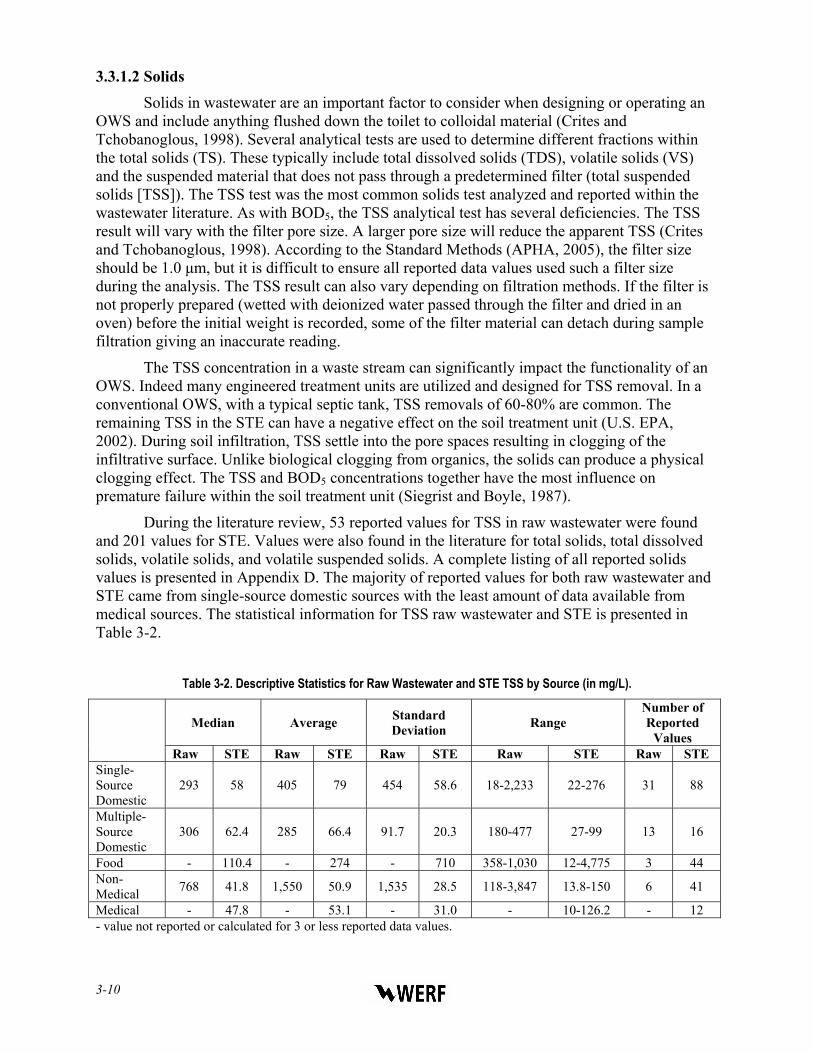
3.3.1.2 Solids
Solids in wastewater are an important factor to consider when designing or operating an OWS and include anything flushed down the toilet to colloidal material (Crites and Tchobanoglous, 1998). Several analytical tests are used to determine different fractions within the total solids (TS). These typically include total dissolved solids (TDS), volatile solids (VS) and the suspended material that does not pass through a predetermined filter (total suspended solids [TSS]). The TSS test was the most common solids test analyzed and reported within the wastewater literature. As with BOD5, the TSS analytical test has several deficiencies. The TSS result will vary with the filter pore size. A larger pore size will reduce the apparent TSS (Crites and Tchobanoglous, 1998). According to the Standard Methods (APHA, 2005), the filter size should be 1.0 μm, but it is difficult to ensure all reported data values used such a filter size during the analysis. The TSS result can also vary depending on filtration methods. If the filter is not properly prepared (wetted with deionized water passed through the filter and dried in an oven) before the initial weight is recorded, some of the filter material can detach during sample filtration giving an inaccurate reading.
The TSS concentration in a waste stream can significantly impact the functionality of an OWS. Indeed many engineered treatment units are utilized and designed for TSS removal. In a conventional OWS, with a typical septic tank, TSS removals of 60-80% are common. The remaining TSS in the STE can have a negative effect on the soil treatment unit (U.S. EPA, 2002). During soil infiltration, TSS settle into the pore spaces resulting in clogging of the infiltrative surface. Unlike biological clogging from organics, the solids can produce a physical clogging effect. The TSS and BOD5 concentrations together have the most influence on premature failure within the soil treatment unit (Siegrist and Boyle, 1987).
During the literature review, 53 reported values for TSS in raw wastewater were found and 201 values for STE. Values were also found in the literature for total solids, total dissolved solids, volatile solids, and volatile suspended solids. A complete listing of all reported solids values is presented in Appendix D. The majority of reported values for both raw wastewater and STE came from single-source domestic sources with the least amount of data available from medical sources. The statistical information for TSS raw wastewater and STE is presented in Table 3-2.
Table 3-2. Descriptive Statistics for Raw Wastewater and STE TSS by Source (in mg/L).
Median Average Standard Deviation Range
Number of Reported
Values
Raw STE Raw STE Raw STE Raw STE Raw STE Single- Source Domestic
293 58 405 79 454 58.6 18-2,233 22-276 31 88
Multiple- Source Domestic
306 62.4 285 66.4 91.7 20.3 180-477 27-99 13 16
Food - 110.4 - 274 - 710 358-1,030 12-4,775 3 44 Non-Medical 768 41.8 1,550 50.9 1,535 28.5 118-3,847 13.8-150 6 41
Medical - 47.8 - 53.1 - 31.0 - 10-126.2 - 12 - value not reported or calculated for 3 or less reported data values.
3-10

Influent Constituent Characteristics of the Modern Waste Stream from Single Sources 3-11
Only three TSS values were reported for raw wastewater food sources and no values were reported for raw wastewater medical sources. The non-medical raw wastewater TSS concentration of 768 mg/L is high compared to the domestic waste sources. However, several of the reported non-medical raw wastewater data values came from an RV dump site, which might lead to a higher concentration of TSS due to the high contribution of toilet waste. STE TSS median values varied between waste stream sources ranging between 41.8 to 155.7 mg/L (Table 3-2). As with BOD5, the median food TSS is over twice as large as any other waste source.
The source of the raw wastewater impacts the TSS concentration. Non-medical values were greater than other source values for all percentiles (Figure 3-4). This trend is again likely attributed to the reported data from the RV dump station included in the non-medical category. As observed with BOD5, TSS raw wastewater trends were similar for single and multiple-source domestic sources with less variability in the multiple-source domestic raw wastewater likely due to homogenization.
For STE, the TSS CFD illustrates a different relationship between waste source than was illustrated for the raw wastewater. The non-medical, medical and single-source domestic STE all had similar trends (Figure 3-5). The food STE TSS concentration was the highest overall.
When comparing the single-source domestic raw wastewater and STE, a TSS trend appears to exist (Figure 3-6). It was expected that the raw wastewater would have higher concentrations compared to STE indicating removal of TSS within the tank. Comparison of the median raw wastewater and STE values suggests 80% removal within the septic tank which is near the upper end of the range of 60-80 % as reported by U.S. EPA (2002). The raw wastewater was found to have higher TSS concentrations than STE for all percentiles with an increased difference at higher percentiles. This might indicate inconsistent removal within the septic tank and increased TSS removal efficiency at higher raw wastewater concentration. Again, because the raw wastewater and STE values shown on Figure 3-6 are from different studies, additional monitoring including raw wastewater and STE concentrations from the same system, and further statistical analysis are required to validate apparent TSS removals.

0
10
20
30
40
50
60
70
80
90
100
0 500 1000 1500 2000 2500 3000 3500 4000 4500
TSS (mg/L)
Cum
ulat
ive
Freq
uenc
y (%
)
Single Source Domestic
Multiple Source Domestic
Non-Medical
Figure 3-4. Raw Wastewater TSS by Source (insufficient data from food and medical sources).
0
10
20
30
40
50
60
70
80
90
100
0 100 200 300 400 500 600 700TSS (mg/L)
Cum
ulat
ive
Freq
uenc
y (%
)
Single Source Domestic
Multiple Source Domestic
Food
Non-Medical
Medical
Value of 4775 mg/L not Shown for Food
Figure 3-5. STE TSS by Source.
3-12

Influent Constituent Characteristics of the Modern Waste Stream from Single Sources 3-13
0
10
20
30
40
50
60
70
80
90
100
0 250 500 750 1000 1250 1500 1750 2000 2250 2500TSS (mg/L)
Cum
ulat
ive
Freq
uenc
y (%
)
STERaw Wastewater
Figure 3-6. Comparison of TSS in Single-Source Domestic Raw Wastewater and STE.
3.3.1.3 Nutrients Nitrogen and phosphorus are the nutrients of interest in raw wastewater and STE due to
potential human health risks and environmental concerns. Of these two nutrients, nitrogen is considered to pose a larger threat due to human health risks and its higher mobility in the environment (Reneau et al., 1989; Siegrist et al., 2001). The major health issue associated with nitrogen is elevated nitrate in drinking water which is thought to cause methemoglobinemia, or blue baby syndrome. Infants are especially susceptible to methemoglobinemia because the pH in the stomach allows for more of the nitrate to be reduced to nitrite. The nitrite binds to the hemoglobin in the blood stream, reducing the oxygen capacity of the blood, eventually leading to asphyxiation. Nitrate is a regulated contaminant in drinking water with a maximum concentration limit of 10 mg-N/L.
Elevated levels of nitrogen can also cause eutrophication (excessive growth of aquatic plants) in receiving bodies of water. Nitrogen is used as a food source for algae. When excess levels of nitrogen are present, algae growth and respiration increases, depleting the water of oxygen which can suffocate the remaining aquatic life. In addition, excess nitrogen leads to development of algal mats on the surface of the water which prevents sunlight from reaching the submerged plants. These submerged plants then cannot respire the much needed oxygen.
Both nitrogen and phosphorus are essential nutrients for plant growth. The portion of total phosphorus that is available for phytoplankton growth is the dissolved reactive phosphorus fraction. Determination of the ratio of nitrogen concentration to phosphorus concentration (N/p ratio) provides an estimation of the limiting nutrient controlling plant growth in surface waters.

Generally, N/p ratios of 20 or more suggest phosphorus limited waters, while N/p ratios of 5 or less suggest nitrogen limited waters (Thomann and Mueller, 1987).
Nitrogen Forms of nitrogen in water and wastewater are: ammonia, nitrite, nitrate, and organic nitrogen. All of these forms of nitrogen as well as nitrogen gas are components of the nitrogen cycle and are of interest for many reasons. In water at pH near 7, about 99% of the ammonia (NH3) molecules are protonated (addition of H+ molecule) forming the ammonium ion (NH4
+). Raw wastewater generally is dominated by the ammonium-nitrogen and organic-nitrogen. Because a septic tank is typically anaerobic (absence of oxygen), conversion of organic-nitrogen to ammonium-nitrogen is rapid and nitrogen remains predominantly as ammonium in STE. Once STE is applied to the soil treatment unit, nitrification occurs (conversion of ammonium to nitrate) if sufficient oxygen along with the proper microbial population are present. Subsequently, if anaerobic conditions and the required microbial population are present, denitrification occurs to convert nitrate to nitrogen gas. The rate of nitrification/denitrification is site-specific and dependent upon other factors such as temperature, organic matter, and water content. Engineered treatment units are often designed for nitrogen removal by nitrifying the ammonium to nitrate through an aerobic process followed by recirculation back into the anaerobic septic tank for denitrification.
Ammonia-nitrogen, nitrate-nitrogen, and nitrite-nitrogen are easily measured colorimetrically. High solids content in the samples may result in interferences with ammonia analyses, but this can be overcome by using other analytical methods. Nitrite-nitrogen is relatively unstable and seldom exceeds 1 mg/L in wastewater or 0.1 mg/L in natural waters (Crites and Tchobanoglous, 1998). Total oxidized nitrogen is also typically analyzed and is the sum of nitrite-nitrogen and nitrate-nitrogen. Total kjeldahl nitrogen is frequently reported for wastewaters. Analytically, organic nitrogen plus ammonia-nitrogen is referred to as kjeldahl nitrogen. If kjeldahl nitrogen and ammonia nitrogen are determined individually, the organic nitrogen is obtained as the difference. Total nitrogen is also frequently reported and includes all of the forms of nitrogen (ammonia, nitrite, nitrate, and organic).
The numerous species of nitrogen make it important to quantify all forms of nitrogen to fully understand what is occurring during the treatment process. During the literature review, all reported nitrogen values were included in the Excel database. Because different forms of nitrogen were reported, incomplete information was available for each nitrogen form. Total nitrogen will be the focus of this section because it can be used to evaluate nitrogen removal during specific treatment processes. In addition, the expected total nitrogen concentration in the raw wastewater is an important OWS design criteria. A complete listing of reported nitrogen values is presented in Appendix E.
During the literature review under 50 values for nitrogen (total nitrogen, kjeldahl nitrogen, ammonia, and nitrate) in raw wastewater were found while over 250 values were found for STE. The majority of reported values for both raw wastewater and STE came from single- source domestic sources. A similar number of total nitrogen values in non-medical STE were found. Table 3-3 presents the statistical information for nitrogen in raw wastewater and STE.
Because the nitrogen values were from different studies, a mass balance for nitrogen can not be completed based on the reported values in Table 3-3. However, the median values appear to coincide with the known relationship between total nitrogen, kjeldahl nitrogen, ammonia-nitrogen and nitrate-nitrogen. The total nitrogen should be approximately equivalent to kjeldahl nitrogen plus nitrate-nitrogen. In the single-source domestic raw wastewater, the median value of kjeldahl nitrogen plus nitrate nitrogen is 62.2 mg-N/L, which is very close to the median total
3-14

Influent Constituent Characteristics of the Modern Waste Stream from Single Sources 3-15
nitrogen value of 63 mg-N/L. Similarly the median total nitrogen value in single-source domestic STE was 55.4 mg-N/L, which is roughly 3 mg-N/L more than the kjeldahl nitrogen and nitrate nitrogen median values added together. Given the analytical error and variability between different studies, the relative closeness of the reported total nitrogen values to the kjeldahl nitrogen plus nitrate-nitrogen values is surprisingly similar and suggests that the median values may be a good representation of the data set.
Table 3-3. Descriptive Statistics for Raw Wastewater and STE Nitrogen by Source (in mg-N/L).
Median Average Standard Deviation Range
Number of Reported
Values
Raw STE Raw STE Raw STE Raw STE Raw STE Single-Source Domestic 63 55.4 87.0 57.7 45.2 17.1 44.1-189 26-124 11 43
Multiple-Source Domestic - 46 - 49.3 - 21.7 - 29.8-75.3 2 4
Food - 86.5 - 75.0 - 36.5 - 24.2-103 - 4 Non-Medical - 84.0 - 83.8 - 33.0 - 7-192 1 41
Total nitrogen
Medical - 45.6 - 55.8 - 30.2 - 28.3-125 - 12 Single-Source Domestic 62 52 78.0 54.2 40.1 14.8 43-123.9 27-94.4 5 25
Multiple-Source Domestic - - - - - - - - 2 2
Food - 71 - 65.6 - 17.3 - 30-82 - 7 Non-Medical - 100 - 233 - 257 - 30-830 3 26
Kjeldahl nitrogen
Medical - - - - - - - - - -
Single-Source Domestic 47.5 36.1 53.4 37.2 37.7 14.8 8.8-154 0-96.2 12 80
Multiple-Source Domestic - 30 - 34.2 - 13.6
8 - 20.1-55 - 7
Food - - - - - - - - - - Non-Medical 178 83 289 186 345 229 32.2-767 19.8-890 4 37
Ammonia nitrogen
Medical - - - - - - - - - - Single-Source Domestic 0.16 0.20 0.49 0.82 0.56 1.9 0.05-1.1 0-10.3 5 45
Multiple-Source Domestic - - - - - - - - - 3
Food - - - - - - - - - - Non-Medical - 0.23 - 0.45 - 0.53 - 0-1.4 1 7
Nitrate nitrogen
Medical - - - - - - - - - - - value not reported or calculated for 3 or less reported data values.
There was not enough data to compare raw wastewater total nitrogen concentrations by waste source (Figure 3-7), but the STE comparison shows that the waste source is important (Figure 3-8). The limited STE data values for multiple-source domestic and food made it difficult to compare to the other sources. The non-medical sources generally had a higher concentration than the single-source domestic in STE. This might be due to the non-medical sources including waste sources such as offices, where the toilet waste contribution to the waste stream would be higher compared to the typical single-source domestic waste stream.

0
10
20
30
40
50
60
70
80
90
100
0 20 40 60 80 100 120 140 160 180 200Total Nitrogen (mg-N/L)
Cum
ulla
tive
Freq
uenc
y (%
)
Single Source Domestic
Other Values Reported:
Multiple Source Domestic: 80 and 39 mg/L
Non-Medical: 38.61 mg/L
Figure 3-7. Raw Wastewater Total Nitrogen.
0
10
20
30
40
50
60
70
80
90
100
0 50 100 150 200 250Total Nitrogen (mg-N/L)
Cum
ulat
ive
Freq
uenc
y (%
)
Single Source DomesticMultiple Source DomesticFoodNon-MedicalMedical
Figure 3-8. STE Total Nitrogen by Source.
3-16

Influent Constituent Characteristics of the Modern Waste Stream from Single Sources 3-17
Phosphorus Phosphorus occurs in natural wastes and wastewaters almost solely as phosphates. Phosphorus can be found in several species including: orthophosphate, polyphosphates, and organic phosphorus (Crites and Tchobanoglous, 1998). Kirkland (2001) reported that in wastewater, about 85% of the total phosphorus is orthophosphate. The organically bound phosphorus is usually of minor importance in most domestic wastes, but can be important in industrial waste and wastewater sludges (Crites and Tchobanoglous, 1998).
As previously discussed, phosphorus is of concern in wastewater as eutrophication can occur with relatively low phosphorus concentrations. The removal of phosphorus can be difficult to achieve on any scale, whether onsite or municipal, due to complex precipitation, adsorption, and desorption reactions that phosphorus undergoes. In conventional OWS, most of the phosphorus removal is achieved by sorption in the soil treatment unit with removal efficiency dependent on specific site conditions. Although OWS currently are not typically regulated for point source discharge of phosphorus, the removal of phosphorus might be an important constituent when designing an OWS system.
The analytical test for total phosphorus converts all of the species into orthophosphate form. Reported values for total phosphorus are assumed to be representative of total phosphates. One issue that occurred during the literature search was the reported units for phosphorus. The most frequently reported analytical result was total phosphorus, but many data values were also reported for orthophosphate or organic phosphorus. Only data values that were reported as total phosphorus are discussed here to ensure all data values were a measure of the same parameter. A complete listing of reported phosphorus values are presented in Appendix E.
Limited data values were found in the literature for total phosphorus. Only a few total phosphorus raw wastewater data values were found with the majority of those from single-source domestic raw wastewater. Single-source domestic raw wastewater was the only waste source to have more than three data values for total phosphorus concentrations. The majority of STE data values were from single-source domestic and non-medical. The food STE total phosphorus concentration was the highest overall median value. The statistical information regarding both raw wastewater and STE concentrations by source is shown in Table 3-4.
Table 3-4. Descriptive Statistics for Raw Wastewater and STE Total Phosphorus by Source (in mg/L).
Median Average Standard Deviation Range
Number of Reported
Values
Raw STE Raw STE Raw STE Raw STE Raw STE Single- Domestic 19 10 19.1 12.2 4.15 7.86 13.05-25.8 3-39.5 8 49
Multiple- Source Domestic
- 6.9 - 7.03 - 1.9 - 5-10 3 6
Food - 17 - 17.9 - 6.85 - 7-28 - 4 Non-Medical - 14 - 21.9 - 23.2 - 4.1-100 1 42
Medical - - - - - - - - - - - value not reported or calculated for 3 or less reported data values.
The literature search did not reveal sufficient raw wastewater total phosphorus values to compare waste sources. However, comparison of all raw wastewater total phosphorus values to

all STE values illustrated on a CFD, indicates a potential relationship for total phosphorus (Figure 3-9). The total phosphorus in raw wastewater was higher than STE except at higher percentiles (>90%). Some phosphorus removal could be expected within the septic tank due to adsorption to solids. Comparison of the median raw wastewater and STE values suggests nearly 50% removal within the septic tank. This might be due to the lack of raw wastewater data values or chemical precipitation reactions that can occur within the septic tank. However, because the raw wastewater and STE values shown on Figure 3-96 are from different studies, additional monitoring including raw wastewater and STE concentrations from the same system, and further statistical analysis are required to validate apparent removals. The STE total phosphorus concentrations appear dependent upon the waste source with the lowest values reported for multiple-source domestic STE (Figure 3-10). The multiple-source domestic STE also appears to have the least variability within the waste stream as illustrated on the CFD.
0
10
20
30
40
50
60
70
80
90
100
0 10 20 30 40 5Total Phosphorus (mg-P/L)
Cum
ulat
ive
Freq
uenc
y (%
)
0
STERaw Wastewater
Figure 3-9. Comparison of Total Phosphorus in Single-Source Domestic Raw Wastewater and STE.
3-18

Influent Constituent Characteristics of the Modern Waste Stream from Single Sources 3-19
0
10
20
30
40
50
60
70
80
90
100
0 20 40 60 80 100 120
Total Phosphorus (mg-P/L)
Cum
ulat
ive
Freq
uenc
y (%
) Single Source DomesticMultiple Source DomesticFoodNon-Medical
Figure 3-10. STE Total Phosphorus by Source (insufficient data for medical sources).
3.3.1.4 Fecal Coliform Fecal coliform bacteria are rod shaped bacteria found in human intestines (Crites and
Tchobanoglous, 1998). Fecal coliform was the most frequent microbial parameter analyzed and reported within the literature. Results are typically reported as colony forming units (cfu) per 100 milliliters ranging over several orders of magnitude. Traditionally, the presence of fecal coliform bacteria has been used as an indicator for the possible presence of pathogenic organisms. Although often reported, the fecal coliform analytical result may not be ideal in characterizing the virus and bacteria in a waste stream. The presence of enteric viruses and protozoa may not correlate with the presence of fecal coliforms, and nonhuman pathogenic organisms can also be found in waste streams (see Section 3.3.2.2 for additional discussion) (Crites and Tchobanoglous, 1998).
Statistical information for fecal coliforms in raw wastewater and STE is presented in Table 3-5. Note, the geometric mean value is reported to better capture small values in the data that range by orders of magnitude rather than the average value which neglect the smaller values. A complete listing of reported fecal coliform values is presented in Appendix F. Limited fecal coliform data values in raw wastewater were found with only single-source domestic values reported. Based on the limited reported fecal coliform data values in raw wastewater, greater uncertainty exists when evaluating the CFD. Fecal coliform values were reported for single- source domestic, multiple-source domestic, and non-medical STE sources.
Figure 3-11 illustrates the CFD for the limited raw wastewater fecal coliform values in comparison to the reported STE values. Comparison of raw wastewater and STE fecal coliform

trends is difficult due to the few reported data values for raw wastewater. Figure 3-12 suggests that fecal coliform concentrations in STE were similar across all waste sources.
Table 3-5. Descriptive Statistics for Raw Wastewater and STE Fecal Coliform by Source (in cfu/100mL).
Median Geometric Mean Range Number of Reported Values
Raw STE Raw STE Raw STE Raw STE Single- Source Domestic
4.9×10⁵ 2.2×10⁵ 4.4×10⁵ 2.2×10⁵ 3.0×10⁴-7.4×10⁶
1.9×10³-1.3×10⁸ 5 65
Multiple- Source Domestic
- 1.1×10⁶ - 7.0×10⁵ 1.4×10⁵-2.7×10⁶ - 5
Food - - - - - - - Non-Medical - 3.7×10⁵ - 3.9×10⁵ 4.1×10⁴-
9×10⁶ - 20
Medical - - - - - - - value not reported or calculated for 3 or less reported data values.
0
10
20
30
40
50
60
70
80
90
100
1.0E+03 1.0E+04 1.0E+05 1.0E+06 1.0E+07 1.0E+08 1.0E+09
Fecal Coliforms (cfu/100ml)
Cum
ulat
ive
Freq
uenc
y (%
)
STERaw Wastewater
Figure 3-11. Comparison of Fecal Coliform in Single-Source Domestic Raw Wastewater and STE.
3-20

Influent Constituent Characteristics of the Modern Waste Stream from Single Sources 3-21
0
10
20
30
40
50
60
70
80
90
100
1.0E+03 1.0E+04 1.0E+05 1.0E+06 1.0E+07 1.0E+08 1.0E+09
Fecal Coliforms (cfu/100ml)
Cum
ulat
ive
Freq
uenc
y (%
)
Single Source DomesticMultiple Source DomesticNon-Medical
Figure 3-12. STE Fecal Coliform by Source.
3.3.1.5 Flow Rate Previous studies have looked extensively into household water use flow rates (Mayer et
al., 1999; Anderson et al., 1993; Anderson and Siegrist, 1989; Brown and Caldwell, 1984). Flow rate is an important parameter when designing an OWS for obvious reasons including treatment unit sizing, estimation of hydraulic loading rates, assessment of peak flow conditions, and estimation of constituent mass loading (e.g., nitrogen, phosphorus). The design for many OWS treatment units must consider the peak flows as well as ensure a safety factor. If the actual flow rate from a structure were to be significantly higher than the design flow, the treatment unit could be undersized leading to poor performance. Alternatively if the actual flow rate was significantly lower than the design flow, the treatment unit could be oversized resulting in unnecessary costs. In other cases, the total mass loading to the environment may be of concern where the mass loading is calculated by multiplying a concentration by flow rate.
Reported median single-source flow rates may not be adequate from a design perspective. A CFD for flow rates enables the user to assess likely flow rates and the degree of uncertainty. For example, an OWS goal may be to limit the impact of nitrogen to groundwater in a sensitive environment. For this example the 80th percentile nitrogen concentration and flow rate might be used. Selection of conservative values for both nitrogen and flow would result in a mass loading that is more conservative than the 80th percentile suggests and some other combination might be appropriate. In either case, the user can select values based on the particular goal.
Limited flow rate data values specific to OWS were found within the literature. Furthermore, of all literature sources reviewed, only 16 studies provided any information related to septic tank configuration and sizing. Of the information found, the majority was from single-
source domestic systems. Non-medical and food sources provided enough data values to provide a source comparison, but only 3 data values were found for multiple-source domestic systems and no values were found for medical sources.
The statistical information for flow rate data found within the literature is shown in Table 3-6. The median value of 161 gpd for single-source domestic systems is comparable to previously reported values. Brown and Caldwell (1984) reported an average flow rate of 66.2 gallons/capita/day for all households, ranging between 77 gallons/capita/day for non conserving households and 59.7 gallons/capita/day for households with water conserving fixtures. In the arid southwest with high outdoor water use, the average water use can be as high as 105-120 gallons/capita/day (Anderson and Siegrist, 1989). According to the American Water Works Association Research Foundation study (Mayer et al., 1999) including over 1100 households, the median indoor flow rate was 60.5 gallons/capita/day, and the average household per capita was 2.8 (the average indoor flow rate was 69.3 gallons/capita/day). By multiplying the median flow rate by the average household per capita, a daily household flow rate of 169 gpd is estimated. Assuming the same median flow rate of 60.5 gallons/capita/day and an average household per capita of 2.6 (U.S. Census Bureau) a household flow rate of 157 gpd is estimated. These estimates are similar to the median value of 161 gpd found within the literature for single-source domestic (Table 3-6).
As the household occupancy increases, the average per capita water use declines due to common household activities such as washing clothes and dishes. Mayer et al., (1999) suggest that the water use increased by approximately 37.2 gallons/capita/day above a common threshold household water use of 69.2 gallons/day. In this case, water use for a household with 5 occupants would be approximately 255 gallons/day (37.2 gallons/capita/day × 5 occupants + 69.2 gallons/day household water use) rather than estimated as 302 gallons/day if the median per capita water use was simply multiplied by the number of occupants (i.e., 60.5 average gallons/capita/day × 5 occupants).
Comparison of estimated flow rates with water conserving fixtures suggests up to 20% or more water savings. Brown and Caldwell (1984) suggest approximately 22% less total water use due to the use of water conserving fixtures. Mayer et al., (1999) evaluated the water savings attributed to ultra low flow toilets and showers. Compared to the average indoor water use, savings of 10.5 gallons/capita/day for ultra low flow toilets and 3 gallons/capita/day for low flow shower heads were observed. Other conservation methods such as running full loads for clothes washers and dishwashers, repair of plumbing leaks, and water use habits (e.g., running water faucet during tooth brushing) would lead to additional water savings.
The CFD for flow rate provides a comparison between single-source domestic, food, and non-medical sources. The non-medical sources had high flow rates at the high percentiles because of the broad range of waste sources. The food flow rate showed some variability because it included data from full service restaurants as well as convenience stores with a quick stop restaurant. The commercial sources are expected to have higher variability within the reported data because of the wide variety of sources included within the groupings. For example, both a five-bedroom and 20-bedroom motel would be included in the non-medical category, even though they are expected to have different flow rates.
3-22

Influent Constituent Characteristics of the Modern Waste Stream from Single Sources 3-23
Table 3-6. Descriptive Statistics for STE Flow Rate by Source (in gpd).
Median Average Standard
Deviation Range Number of Reported
Values Single-Source Domestic 161 184 84.8 62.9-388 30
Multiple- Source Domestic
- - - - 3
Food 353 814 1,079 73.2-3,791 12 Non-Medical 234 1,554 3,056 30-14,100 26 Medical - - - - - - value not reported or calculated for 3 or less reported data values.
0
10
20
30
40
50
60
70
80
90
100
0 1000 2000 3000 4000 5000 6000Flow Rate (gpd)
Cum
ulat
ive
Freq
uenc
y (%
)
Single Source Domestic
Food
Non-Medical
Value of 14,100 gpd Not Used for Non-Medical
Figure 3-13. STE Flow Rate by Source.
3.3.1.7 Other Constituents Values were found in the literature for pH, alkalinity, chemical oxygen demand, total
organic carbon, and chloride. However, these other constituents were reported sporadically which prevents detailed analysis of descriptive statistics or CFDs. A complete listing of these other constituents is presented in Appendix I.

3.3.2 Tier 2: Oil and Grease and Microbial Constituents
The following sections provide a summary of the literature review results for oil and grease, and microbial constituents of interest. The information is presented first in table format to give the statistical information for each source. The data values are then presented in CFDs to evaluate how raw wastewater and STE vary by constituent, as well as by the wastewater source.
3.3.2.1 Oil and Grease Oil and grease is typically used to describe the fats, oils, waxes, and other related
constituents found in wastewater. Oil and grease are composed of esters from alcohol or glycerol from fatty acids (Crites and Tchobanoglous, 1998). The presence of oil and grease within an OWS can be detrimental to treatment processes due to accumulation and interference with biological processes.
The literature search found limited data values for oil and grease concentrations in both raw wastewater and STE. Data values were found for single-source domestic, food, and non-medical. The statistical information for oil and grease within raw wastewater and STE is found in Table 3-7.
The oil and grease concentrations in raw wastewater and STE by source are shown in Figure 3-14. Insufficient data were available to illustrate raw wastewater by source. The STE data values for food, and non-medical indicate that the source, as expected, affects oil and grease concentration, due to the high oil and grease content of food waste.
Table 3-7. Descriptive Statistics for Raw Wastewater and STE Oil and Grease by Source (in mg/L).
Median Average Standard Deviation Range
Number of Reported
Values
Raw STE Raw STE Raw STE Raw STE Raw STE Single- Source Domestic
73.5 - 73.3 - 39.3 - 16-134 - 14 3
Multiple- Source Domestic
- - - - - - - - - -
Food - 48 - 66.9 - 59 - 9-300 - 36 Non-Medical - 40 - 50.1 - 44.2 - 6-140 2 15
Medical - - - - - - - - - - - value not reported or calculated for 3 or less reported data values.
3-24

Influent Constituent Characteristics of the Modern Waste Stream from Single Sources 3-25
0
10
20
30
40
50
60
70
80
90
100
0 50 100 150 200 250 300Oil and Grease (mg/L)
Cum
ulat
ive
Freq
uenc
y (%
)
STE Food
STE Non-Medical
Raw Single Source Domestic
Figure 3-14. STE Oil and Grease Concentration by Source.
3.3.2.2 Microbial Constituents Raw wastewater as well as STE is known to contain many microorganisms (i.e. bacteria,
virus, and protozoa), both harmless and pathogenic (disease causing). From a human health perspective, the release of pathogenic organisms may have a profound impact. Several outbreaks of disease have been documented and attributed to the release of human pathogens to wastewater and subsequent exposure and infection of others (McGinnis and DeWalle, 1982). It is important to note that not all viruses and bacteria are harmful; in fact, the majority are actually beneficial to human health. In addition to being beneficial or essential to human health, microorganisms are also important for proper OWS function. A wide array of microorganisms can be found in wastewater, but much of the research on these microorganisms focuses on eliminating them as possible contaminants of groundwater. In addition, research typically has focused on centralized wastewater treatment plants and their treated effluent. Thus, little has been done to characterize the microbial community of OWS raw wastewater from single sources. Although it is essential to characterize any organisms present after treatment and dispersal in the environment, it is also important to characterize prior to any treatment. Characterizing raw wastewater from single sources will provide a better understanding of potential risks and may allow more appropriate treatment methods to be implemented.
Background Bacteria are the best-studied group of microorganisms found in wastewater, which is quite evident through the numerous standard analytical methods for detection. Bacteria are single-celled organisms with no membrane-enclosed nucleus or other organelles (prokaryotic), and usually have their deoxyribonucleic acid (DNA) in a single circular molecule (Madigan et al., 1997). Bacteria range in size from about 0.2 μm-2.0 μm in diameter.

In addition to the human health concerns, bacteria are essential for the proper functioning
of OWS. In a conventional OWS, the septic tank allows for some anaerobic carbon digestion. This process involves the conversion of organic matter to less complex compounds including, methane (CH4), carbon dioxide (CO2), hydrogen (H2), ammonia (NH3), and hydrogen sulfide (H2S) (see Equation 3.1). Bacteria are responsible for much of the digestion and thus removal of organic compounds, and are also responsible for much of the nutrient cycling that occurs in OWS prior to and after release to the environment. Many factors affect digestion including temperature, retention time, and pH (Bitton, 1999). At this time, little is known about the specific roles of specific microorganisms in septic tank digestion. However, several groups of organisms have been found to act in a synergistic manner within the septic tank. Hydrolytic bacteria breakdown complex organic molecules into amino acids, glucose and fatty acids; fermentative acidogenic bacteria convert sugars, amino acids and fatty acids to organic acids, alcohols and ketones, hydrogen, carbon dioxide and acetate; acetogenic bacteria convert fatty acids and alcohols into acetate, hydrogen and carbon dioxide; and methanogens convert hydrogen and carbon dioxide or acetate into methane (Bitton, 1999). The overall anaerobic digestion reaction (Bitton, 1999) is described in equation 3.1.
Organic matter CH4 + CO2 +H2 + NH3 + H2S eqn. 3.1
The presence of viruses in wastewater is of increasing concern. Viruses are much smaller than bacteria at 0.01 μm-0.10 μm in size. They are obligate intracellular parasites that are dependent on host cells for metabolic and reproductive needs; they replicate only inside a living host (Hass et al., 1999). They consist of a strand of either DNA or ribonucleic acid (RNA) inside a protein covering called a capsid. Viruses are not well-characterized, are difficult to detect, and often even more difficult to treat. They are frequently host-cell specific, meaning they will only replicate inside a specific cell type.
Finally, another class of organisms that has recently gained interest is the protozoan parasites. These organisms are single-celled, eukaryotic organisms (cellular organisms having a membrane-bound nucleus). Protozoa are generally much larger than bacteria and range in size from 10 μm-100 μm in diameter.
Pathogens in Wastewater Human fecal matter contains an average of 1012 bacteria per gram, which represents approximately 9% of the feces weight (Dean and Lund, 1981). Of these bacteria, humans shed about 2 × 10⁹ coliforms/day/capita (Bitton, 1999). Coliform bacteria are members of the family Enterobacteriaceae, and are commonly found in the intestinal tracts of warm-blooded animals. They are not all of fecal origin, however. In sanitary bacteriology, these organisms are defined as aerobic (grow in the presence of oxygen) or facultative anaerobic (grows in the presence or absence of oxygen), gram-negative, nonspore-forming, rod-shaped bacteria that ferment lactose with gas and acid formation within 48 hours at 95°F (35°C). Fecal coliform bacteria are members of the total coliform group of bacteria but are characterized by their ability to ferment lactose at 112.1°F (44.5°C). Both coliforms and fecal coliforms are often considered “indicator” organisms. That is, they commonly indicate contamination of soil or water by human waste (and potentially pathogens) as they are found in large quantities in human fecal matter. These organisms are considered part of the normal human flora (they are expected to be present, and may be useful or essential for human survival) and generally do not cause disease. However, fecal coliforms are considered more specific indicators of fecal contamination than are coliforms that ferment lactose only at 95°F(35°C), because they are exclusively found in intestinal tracts. There is probably no universal indicator organism for determining contamination; under different conditions, different organisms may be better indicators than
3-26

Influent Constituent Characteristics of the Modern Waste Stream from Single Sources 3-27
others may. Escherichia coli and some Klebsiella pneumoniae strains are the principal fecal coliforms of interest and are easily cultured. Much of what we know of microorganisms in raw wastewater and STE stems from enumeration of these indicator organisms. Table 3-8 shows a variety of bacterial concentrations found in STE by several investigators. Table 3-9 illustrates the range of concentrations of microorganisms that may be found in raw wastewater and/or STE.
Table 3-8. Literature Values for Concentration of Select Microorganisms Found in STE.
Organism/Organism Type Mean cfu1/100ml or pfu2/100ml Fecal Coliforms 1.1 × 10⁶ (Brown et al., 1980)
4.2 × 10⁵ (Ziebell et al., 1977) 1.9 × 10⁶ (Ziebell et al., 1977) 4.2 × 10⁵ (McCoy and Ziebell, 1975)
Coliphages/Viruses 6.4 × 101 (Brown, et al., 1980) Total Coliforms 3.4 × 10⁶ (Ziebell et al., 1977)
5.7 × 10⁶ (Ziebell et al., 1977) Fecal Streptococci 3.8 × 10³ (Ziebell et al., 1977)
1.6 × 10⁵(Ziebell et al., 1977) 3.8 × 10³ (McCoy and Ziebell, 1975)
Total Bacteria 3.4 × 10⁶ (Ziebell et al., 1977) 3.0 × 10⁷ (Ziebell et al., 1977) 3.4 ×10⁸ (McCoy and Ziebell, 1975)
1 cfu, colony forming units; refers to bacterial counts 2 pfu, plaque forming units; refers to viral counts
Table 3-9. Microorganism Concentration Found in Raw Wastewater and STE. 1
Organism Concentration found in raw wastewater and STE (MPN/100 mL)2
Bacteria Total Coliform Fecal Coliform Clostridium perfringens Enterococci Fecal streptococci Pseudomonas aeruginosa Shigella Salmonella
107-1010 106-108 103-105 104-105 104-106 103-104 100-103 102-104
Viruses Enteric virus Coliphage
103-104 103-104
Protozoa Cryptosporidium parvum oocysts Entamoeba histolytica cysts Giardia lamblia cysts
101-104
10-1-103
103-104 1 Adapted from Crites and Tchobanoglous (1998) and U.S. EPA (2002) 2 Most probable number per 100 mL
Pathogenic bacteria found in wastewater include Salmonella typhi, Shigella, Vibrio cholerae, pathogenic E. coli, Legionella pneumophila, Mycobacterium tuberculosis, Leptospira, and Helicobacter pylori (Crites and Tchobanoglous, 1998; Bitton, 1999); these and other

wastewater pathogens, and the diseases they cause, are summarized in Table 3-10. All of these organisms have the potential to infect exposed humans. Salmonella spp. are the most predominant pathogenic bacteria found in wastewater and can range in numbers from just a few organisms to 8,000 organisms/100 mL (Crites and Tchobanoglous, 1998; Bitton, 1999). Ziebell and others (1977) found, along with high coliform, fecal streptococci and Pseudomonas aeruginosa counts, Salmonella in 59% of 17 different septic tank pumpout sludges.
In human waste, 100 types of virus have been detected (Gerba and Bitton, 1984). Most individuals have at least one viral infection per year, so it is likely that wastewater systems will receive virus-laden waste at some point over a given year (Gerba, 2002). The following viruses have been found in fecal specimens: poliovirus, ECHOvirus, coxsackie virus, enterovirus, Norwalk virus, and adenovirus (Table 3-10). Additionally, HIV has been isolated from wastewater; however, there is no evidence of its transmission via this route. Hepatitis A has also been found and is of greatest concern due to its disease severity and potential to survive for long periods in soil (Bitton, 1999).
Table 3-10. Pathogenic Microorganisms found in Raw Wastewater and STE. 1
Organism Disease Caused Symptoms Bacteria
Salmonella typhi Shigella Vibrio cholerae Yersinia enterocolitica E. coli (pathogenic) Legionella pneumophila Leptospira spp. Campylobacter jejuni
Typhoid fever Bacillary dysentery Cholera Gastroenteritis Gastroenteritis Legionnaires’ disease Weil’s Disease Gastroenteritis
High fever, diarrhea Dysentery Diarrhea, dehydration Diarrhea Diarrhea Malaise, acute respiratory illness Jaundice, fever Diarrhea
Virus Adenovirus Enteroviruses Poliovirus Echovirus Coxsackie virus Hepatitis A Norwalk Parvovirus Rotavirus HIV
Respiratory disease Gastroenteritis,
meningitis, heart anomalies
Infectious hepatitis Gastroenteritis Gastroenteritis Gastroenteritis AIDS
Jaundice, fever Vomiting Diarrhea Diarrhea
Protozoa Cryptosporidium parvum Giardia lamblia Balantidium coli Entamoeba histolytica Cyclospora
Cryptosporidiosis Giardiasis Balantidiasis Amoebic dysentery Cyclosporasis
Diarrhea, low-grade fever Diarrhea, nausea, indigestion Diarrhea, dysentery, intestinal ulcers Diarrhea, dysentery Severe diarrhea, nausea, vomiting, severe
stomach cramps 1 Partially adapted from Bitton (1999) and from Crites and Tchobanoglous (1998)
Protozoa cause a number of diseases, such as African sleeping sickness, malaria, and dysentery. Several pathogenic protozoa have been detected in wastewater, including Cryptosporidium parvum, Cyclospora, and Giardia lamblia (Crites and Tchobanoglous, 1998). These organisms may have a significant impact on children, elderly and immuno-compromised individuals.
3-28

Influent Constituent Characteristics of the Modern Waste Stream from Single Sources 3-29
Detection Methods Several methods are available for detection of bacteria in wastewater samples (APHA, 2005). By far, detection of indicator organisms (coliforms and fecal coliforms) is the most common and well understood. Bacteria can be enumerated/detected using several methods: direct count, membrane filtration, multiple tube fermentation, and plate culture methods (Crites and Tchobanoglous, 1998; APHA, 2005). Direct counts are obtained microscopically using a counting chamber. One drawback to direct counts is that it is impossible to differentiate between live and dead cells. With the membrane filtration technique, a known volume of water is passed through a membrane filter and bacteria are retained on the filter. The filter is then placed in contact with agar that contains the appropriate nutrients for growth. The bacteria are then incubated and colony-forming units can be counted to determine the concentration found in the sample. Advantages to this technique include its ability to directly count coliform bacteria and its ease of analysis. Multiple tube fermentation is a tedious method that often over-estimates the number of organisms present (Crites and Tchobanoglous, 1998). Concentrations of bacteria are reported as the most probable number per 100 mL (MPN/100 mL) and are obtained by the analysis of positive and negative results of the test. Plate culture methods involve dilution of samples and subsequent culturing in petri dishes containing nutrient agar. Distinct colonies seen on the agar after incubation are counted to determine the concentration in the original sample. This method is extremely sensitive, but depending on the nutrients added to the agar may not differentiate groups of bacteria. With the latter three methods, it is important to note that only a small fraction of organisms can actually be cultured in the laboratory.
Although fecal coliforms are indicators for the potential presence of pathogenic bacteria, they may not be indicators of the presence of pathogenic viruses or protozoa. Due to their size, survivability, and surface properties, the behavior of fecal coliform bacteria may not adequately mimic that of viruses (Van Cuyk et al., 2004). Attention is now being focused on detection of bacteriophages as indicators of virus presence. Bacteriophages are viruses that infect bacterial cells and may be shed in feces along with their bacterial hosts. The most common means of detection of bacteriophages is via a double-layer plaque assay (APHA, 2005).
Detection of viruses can be quite difficult due to several factors. Virus concentrations are generally low, thus the first problem is concentrating the virus sufficiently for detection and enumeration. Concentration methods include ultracentrifugation (requires expensive equipment), dialysis, and adsorption to sediment particles (appears to offer protection against inactivation (Atlas and Bartha, 1998). For detection, viruses must be grown in suitable host cells, specific for individual virus types. Thus, the target virus of interest must be known before detection methods can be implemented.
Microbial Fate and Transport The main route of infection by such pathogens is the fecal/oral route, thus exposure to raw wastewater or STE is of primary concern. For this reason, much attention is paid to the fate of organisms as they leave the septic tank (Table 3-11). Removal of pathogens is often accomplished by soil filtration, adsorption, desiccation, radiation, predation, and exposure to adverse conditions (Crites and Tchobanoglous, 1998). Areas of focus include microbial transport and removal through soils (Gilbert et al., 1976; McGinnis and DeWalle, 1982; Stewart and Reneau, 1983; Hagedorn, 1984; Converse et al., 1992; Kanter et al., 1998). These focus areas as well as microbial source tracking are important when examining groundwater and surface water contamination.

Table 3-11. Onsite Wastewater Microbial Research Focus.
Organism Research Focus Reference Bacteria
Fecal and total coliform Coliform, streptococci, and P.
aeruginosa Fecal and total coliform, P.
aeruginosa, S. aureus, Salmonella (spp.)
C. perfringens, fecal coliform, and E. coli
Salmonella (spp.) Sulfur oxidizing bacteria Fecal coliform Bacterial review Bacterial review Salmonella typhi Fecal coliform
Impact of water conservation on fecal and total coliform concentrations in STE
STE and soil concentrations Bacterial numbers in STE Bacterial numbers in treatment plant Bacterial numbers in soil Mound system using bacteria for denitrification Transport through soil Survival and transport through soil Transport through soil Transport through soil Concentration with depth below at-grade OWS
Cole and Sharpe, 1983 Ziebell et al., 1977 McCoy and Ziebell, 1975 Lisle et al., 2004 Gilbert et al., 1976 Kanter et al., 1998 Stewart and Reneau, 1983 Gerba and Bitton, 1984 Hagedorn, 1984 McGinnis and DeWalle,
1982 Converse et al., 1992
Virus HIV Enterovirus Hepatitis A Polio virus Coliphage Polio virus Reovirus, enterovirus, and
adenovirus Rotavirus Coliphage Coliphage Coliphage- PRD1 Enterovirus Polio virus Tracer virus Tracer virus- MS-2 and PRD1
Detection in raw wastewater Feces analyzed concentration and STE
concentrations Virus degradation mixed waste Concentrations in mixed waste Concentrations in cluster system and transport
in soil Inactivation in wastewater sludge Concentrations in wastewater treatment plant Detection in raw sewage and creeks Concentrations in wastewater Fate and transport, STE concentrations Removal of PRD1 in septic tank drainfield,
tracer test Transport through soil Transport in sand columns Tracer transport through soil Tracer transport through sand packed 3-D tanks
Ansari et al., 1992 Anderson and Lewis,
1992 Deng and Cliver, 1995b Snowden et al., 1989 Brown et al., 1980 Ward et al., 1976 Sedmak et al., 2005 Mehnert and Stewein,
1993 Goya et al., 1980 Hinkle et al., 2005 Nicosia et al., 2001 Anderson and Lewis,
1992 Green and Cliver, 1977 Yates and Yates, 1997;
Rose et al., 1999 Van Cuyk et al., 2004
Protozoa Giardia Cryptosporidium parvum
Degradation in mixed waste Transport in sand filters
Deng and Cliver, 1995a; Snowden et al., 1989
Logan et al., 2001
Upon application of OWS effluent to the soil infiltrative surface, viruses may be more mobile than bacteria counterparts and thus persistent in the soil partially due to their size. Viruses die or become inactivated (no longer able to replicate inside a host cell) by damage to their structural integrity (Hass et al., 1999), but are not impacted by nutrient deprivation. Studies have focused on viral transport through soils (Gerba, 1989; Anderson et al., 1992; Bechdol et al., 1995; Yates and Yates, 1997; Van Cuyk, 2003; Van Cuyk et al., 2004) and survival in soils and
3-30

Influent Constituent Characteristics of the Modern Waste Stream from Single Sources 3-31
wastewater (Ansari et al., 1992; Lago et al., 2003) due to their potential as contaminants to groundwater. Because viruses themselves do not metabolize or respire, they can often survive long periods outside of the host. Because the cells (hosts) needed for replication of human pathogenic viruses are present in low concentrations in ground water systems, it is often assumed that long-term transport of virus is unlikely. However, Keswick et al. (1982) showed that poliovirus, coxsackie virus and rotavirus survive much longer in the subsurface environment- on the order of weeks and months- than had generally been assumed. Additional research has been done to create a link between episodic virus release and survival within the septic tank. Anderson et al., (1992) found on several occasions residents shedding viruses for up to 30 days. The same viruses identified in feces were identified in the STE.
The goal of microbial source tracking is to distinguish between sources of microbial contamination, in order to effectively direct mitigation efforts (Albert et al., 2003). Most microbial source tracking relies on the use of genetic biomarkers of individual microorganism that are specific for a host population. There is an obvious need to reduce the potential for human exposure to pathogens that may be discharged in to the soil environment and to determine the origin of contamination.
Environmental Impact Microorganisms are most often examined from a human health standpoint rather than their impact on the environment into which they are released. Although of secondary importance at this time, the release of pathogenic organisms into the environment may have a more dramatic effect than we have yet to realize. For example, natural soils can contain 106-109 autochthonous microorganisms (indigenous to a given ecosystem) per gram of soil; if other allochthonous microorganisms (“foreign” to the ecosystem) are released into this environment, they may have an effect on the ecology of the system (Atlas and Bartha, 1998). Autochthonous organisms may be out competed for resources by these allochthonous individuals, leading to an alteration of the soil community. Autochthonous soil microorganisms play an important role in organic matter decomposition and mineral cycling. They are essential for maintaining fertile soils for plant growth and thus directly affect primary productivity (conversion of carbon dioxide to organic carbon) (Atlas and Bartha, 1998).
Characterization of the microorganisms present in raw wastewater and septic tank effluent is critical to understanding their roles in OWS function as well as their potential human health impact and environmental impact. Identification of indicator organisms is important for determining potential contamination but should be coupled with detection of pathogens to gain more insight for human health risk assessment. Pathogens have been identified in wastewater on numerous occasions, but the frequency of occurrence and their fate is not well understood. Characterizing the microbial community of raw wastewater is essential to understanding the impact microorganisms may have on humans as well as the environment.

3.3.3 Tier 3: Trace Organic Wastewater Constituents
The occurrence and fate of pharmaceuticals, consumer product chemicals, and other trace organic wastewater contaminants in the environment has received increasing attention worldwide in the last decade due to the potential adverse effects on ecosystems and human health. Thousands of synthetic organic chemicals are produced each year worldwide for use in industrial and domestic products. In addition, natural organic compounds present in plants and animals may enter the environment through excretion. Chemical groups include polycyclic aromatic hydrocarbons (PAHs), polychlorinated biphenyls (PCBs), dioxins and furans, phthalates, and phenols. These chemicals are used in many categories of organic wastewater contaminants, including non-prescription drugs, antibiotics, reproductive hormones, natural hormones, surfactants, plasticizers, antioxidants, steroids, disinfectants, fire retardants, fragrances, solvents, and pesticides. Some organic wastewater contaminants, such as pharmaceuticals, are designed to elicit a dosed biochemical effect, however they may be incompletely metabolized and enter the environment at biochemically-active levels. Other organic wastewater contaminants have unintentional effects or are degraded to metabolites with more toxic properties than their parent compound. For example, studies have reported hormonally mediated toxic effects, such as elevated levels of vitellogenin, an egg yolk precursor, in fish living in streams impacted by organic wastewater contaminants (Sumpter and Jobling, 1995). Concentrations as low as 10 μg/L of 4-nonylphenol, a detergent surfactant metabolite, inhibited testes growth in rainbow trout (Jobling et al., 1996). Adverse effects have been observed in fish exposed to stream water from Boulder Creek, Colorado, impacted by organic wastewater contaminants (Vajda et al., 2005). These effects include higher proportions of female and intersex fish, gonadal morphology abnormalities, and compromised reproductive potential. The increased use of antimicrobial agents in household cleaning agents, appliances, and clothing has led to concern over the development of antimicrobial-resistant bacteria (Schweizer, 2001).
Wastewater is a primary source of trace organic contaminants to the environment. A number of these compounds are released into the environment after passing through wastewater treatment plants (WWTPs), which are not designed to remove them from the effluent (Kolpin et al., 2002). Several studies (Glassmeyer et al., 2005; Kolpin et al., 2002; Desbrow et al., 1998; Ternes et al., 1999 I and II; Sekela et al., 1999) have reported the occurrence of organic wastewater contaminants in the influents and effluents of municipal WWTPs and explored the fate of these chemicals in some treatment operations (e.g., Giger et al., 1984; Ball et al., 1989; Barber et al., 2000; Belfroid et al., 1999; Sakai 1999; Ternes et al., 1999 I and II; Kolpin et al., 2002). Table 3-12 presents examples of reported concentrations of select organic wastewater contaminants in WWTP influent and effluent. While the source of organic wastewater contaminants to urban streams may be through municipal WWTP discharge, the source of contamination to private domestic wells may be from agriculture, urban development, or through the discharge of treated effluent from OWS to subsurface soils with eventual groundwater and/or surface water recharge.
3-32

Influent Constituent Characteristics of the Modern Waste Stream from Single Sources 3-33
Table 3-12. Example of Occurrence (μg/L) of Select Organic Wastewater Contaminants in WWTP Influent and Effluent.
Influent Effluent Max Med Max Med Compound Common Use
Location (number of
samples) Range Range Reference
Acetaminophen antipyretic U.S. (11) - 1.06 0.006 Glassmeyer et al., 2005 U.S. (11) - 0.31 0.12 Glassmeyer et al., 2005 U.S. (8) - nd-2.7 Barber et al., 2000 Bisphenol A plasticizer U.S. (4) 0.094-0.15 - Rudel et al., 1998 U.S. (11) - 7.99 0.053 Glassmeyer et al., 2005 Caffeine stimulant U.S. (8) - 0.12-4.0 Barber et al., 2000
Carpamazepine antiepileptic U.S. (11) - 0.27 0.08 Glassmeyer et al., 2005 Germany (16) - 0.003 <RL Ternes et al., 1999
17-β-Estradiol reproductive hormone Canada (10) - 0.064 0.006 Ternes et al., 1999
Germany (16) - 0.07 0.009 Ternes et al., 1999 Estrone reproductive hormone Canada (10) - 0.048 0.003 Ternes et al., 1999
Germany (16) - 0.015 0.001 Ternes et al., 1999 Ethynylestradiol ovulation inhibitor Canada (10) - 0.042 0.009 Ternes et al., 1999
Ethylenediaminetetra-acetic acid (EDTA)
metal chelating agent U.S. (8) - 132-439 Barber et al., 2000
U.S. (8) - 0.90-23 Barber et al., 2000 4-Nonylphenol surfactant metabolite U.S. (2) 25-33 - Rudel et al., 1998
U.S. (8) - Barber et al., 2000 4-Nonylphenoldi-ethoxycarboxylate (NP1EC)
surfactant metabolite U.S. (2) 1.3-1.7 Rudel et al., 1998
U.S. (11) - 38 2.2 Glassmeyer et al., 2005 U.S. (8) - 1.5-55 Barber et al., 2000 4-Nonylphenoldi-
ethoxylate (NP1EO) surfactant metabolite
U.S. (2) 15-21 - Rudel et al., 1998 4-Nonylphenolmono-ethoxycarboxylate (NP2EC)
surfactant metabolite U.S. (8) - 16-120 Barber et al., 2000
U.S. (11) - 18 0.88 Glassmeyer et al., 2005 U.S. (8) - 0.78-110 Barber et al., 2000 4-Nonylphenolmono-
ethoxylate (NP2EO) surfactant metabolite
U.S. (2) 6.4-8.0 - Rudel et al., 1998 Sulfamethoxazole antibiotic U.S. (11) - 0.589 0.15 Glassmeyer et al., 2005 Triclosan antimicrobial U.S. (11) - 1.6 0.25 Glassmeyer et al., 2005
Max - maximum concentration; Med - median concentration; - not measured; nd - not detected at ~0.01 mg/L; <RL – less than the reporting level
While much is known about the characteristics and performance of OWS with respect to conventional pollutants, there is almost no information regarding the occurrence and fate of organic wastewater contaminants in these systems and the potential for adverse impacts on receiving waters to which they discharge. However, OWS may treat more variable and potentially higher-strength effluent with respect to organic wastewater contaminants. A WWTP receives wastewater each day from a variety of sources that buffers the system from individual high strength inputs and produces a relatively constant raw wastewater and effluent composition over time. In contrast, OWS waste stream composition is directly affected by water use and waste load characteristics at the individual source or small cluster of sources. Variations occur due to a number of factors, including differences in activities using consumer product chemicals (i.e. presence or absence of a prescription drug-consuming occupant), the proportion each activity contributes to the daily wastewater flow (i.e. household vs. commercial cleaning

frequency), and the volume treated by the system, which is correlated to the number of occupants and may fluctuate over time (i.e. morning vs. mid-day water use in a residence, Sunday church service vs. a weekday, school year vs. summer vacation).
Vast improvements in instrumentation and methodology in the last few decades have made possible quantifiable identification of compounds at trace levels, in the microgram and nanogram per liter range, and even down to picogram per liter levels in clean environmental matrices. Methods using solid-phase extraction, liquid-liquid extraction, or derivatization followed by analysis by high performance liquid chromatography (HPLC) or gas chromatography coupled with mass spectrometry (GC/MS and GC/MS/MS) are becoming more established (Zaugg et al., 2001; Meyer et al., 2000; Vanderford et al., 2003; Cahill et al., 2004), allowing for the analysis of large numbers of samples with reproducible results in all environmental matrices. The complex composition of OWS effluent pushes the limit of quantification of organic wastewater contaminants using these developing analytical methods. However, knowledge of the wastewater source (residential vs. restaurant) and treatment type (conventional septic tank vs. engineered treatment unit) will aid in appropriate sample preparation for quantification of organic wastewater contaminants.
Due to the complex nature of raw wastewater and the continuing development and establishment of methodology, the occurrence of organic wastewater contaminants in OWS raw wastewater has not been quantified to date. Interest in the occurrence and fate of “priority pollutants” by the Environmental Protection Agency (EPA) in the 1980s led to quantification of select volatile organic compounds (VOCs) in OWS, including raw wastewater (DeWalle et al., 1980; Viraraghavan and Hasham, 1985). VOCs were detected including toluene (up to 320 μg/L), benzene (15 μg/L), and additional compounds at low concentrations (<5 μg/L) including dichloromethane, benzene, chloroform, bromodichloromethane, tetrachloroethene, and ethylbenzene. No other known studies have quantified the occurrence of organic wastewater contaminants in OWS raw wastewater.
While few studies have quantified VOCs in raw wastewater, more studies have identified these compounds in STE. Toluene, chloroform, methylene chloride and 1.4-dichlorobenzene were routinely detected in STE samples from eight single-family homes in Florida (Ayres Associates, 1989; Sherman and Anderson, 1991). A septic tank serving 97 single-family homes in western Washington, U.S., identified toluene (average concentration = 39 μg/L) as the most frequently detected priority pollutant, as well as methylene chloride, chloroform, tetrachloroethene, and benzene in concentrations ranging from 1 to 4 μg/L (DeWalle et al., 1980). A similar suite of substituted benzenes (i.e. chloroform, bromodichloromethane, toluene, benzene, methylene chloride, tetrachloroethylene) was identified in STE in Regina, Saskatchewan, Canada (Viraraghavan and Hasham, 1986). Ten of 45 VOCs were detected in STE serving 5 communities and 1 mobile home (Greer and Boyle, 1987). The most frequently detected compounds were toluene (30-200 μg/L) and 1,4-dichlorobenzene (2.2-39 μg/L); other detections included 1,1,1-trichloroethane, tetrachloroethylene, xylenes, ethylbenzene, 1,2-dichloroethane, chloroform, benzene, and carbon disulfide.
In addition to VOCs, research has focused on the occurrence and fate of surfactants in laundry detergents such as linear alkylbenzene sulfonate (LAS). For example, organic compounds occurred in the STE of an OWS serving a single-family home in Cambridge, Ontario at concentrations ranging from microgram to milligram per liter levels (LAS = 10 mg/L, nitrilotriacetic acid = 2 mg/L, ditallow dimethyl ammonium chloride = 4570 μg/L, many substituted benzenes ~5-10 μg/L) (Shimp et al., 1994; Robertson, 1994; McAvoy et al., 1994).
3-34

Influent Constituent Characteristics of the Modern Waste Stream from Single Sources 3-35
More recently, LAS (9.5-18.1 mg/L), alcohol ether sulfate (4.13-5.46 mg/L), and alcohol ethoxylate (0.44-0.94 mg/L) were identified in STE serving a single-family home in Jacksonville, Florida, U.S. (Neilsen et al., 2002).
Advances in extraction methods and chromatographic analyses have allowed for the recent quantification of large suites of trace organic wastewater contaminants in complex matrices such as OWS waste streams. Eriksson et al., (2003) analyzed grey wastewater (from shower and bathroom sink water only, excluding toilet or other household waste) and identified over 200 organic wastewater contaminants including surfactants, emulsifiers, fragrances and flavors, preservatives and antioxidants, softeners and plasticizers, UV filters, solvents, and miscellaneous compounds. Half of the compounds identified were long-chain fatty acids and their esters (i.e. hexanoic acid, octanoic acid, decanoic acid) which are commonly used as surfactants. These compounds also had the highest quantified concentrations, with the highest concentration exceeding 15,000 μg/L (9-octadecenoic acid). In contrast, low levels of chlorophenols, phthalates, and substituted benzenes were generally found.
Rudel et al., (1998) analyzed composite STE from residential sources for phenolic compounds. Nineteen of 20 organic wastewater contaminants were identified, including the endocrine disruptors nonylphenol (1000-1500 μg/L), octylphenol (35-42 μg/L), and bisphenol A (0.11-1.7 μg/L). In comparison, the same study identified WWTP influent concentrations ranging from 25-33 μg/L for nonylphenol, 0.20 to 0.74 μg/L for octylphenol, and 0.094 to 0.15 μg/L for bisphenol A, suggesting concentrations of some organic wastewater contaminants are higher in OWS influents than in WWTP influents.
Eighteen of 22 pharmaceuticals were detected in OWS STE serving residential sources and a school (Godfrey, 2004). The most frequently detected compounds were acetaminophen (up to 1530 μg/L), caffeine (877 μg/L), nicotine, 1,7-dimethylxanthine (910 μg/L), cotinine, warfarin, codeine, trimethoprim, and carbamazepine. The results agreed well with a study that identified 8 of 18 pharmaceuticals in STE from a senior center in La Pine, Oregon, including acetaminophen (120 μg/L), caffeine (110 μg/L), and 1,7-dimethylxanthine (58 μg/L) (Hinkle et al., 2005). In the same study, 45 of 63 organic wastewater contaminants were detected in 21 STE samples serving single-family homes and the senior center. Fourteen of the 45 were detected in greater than 90% of the samples, including 4-methylphenol (max = 1300 μg/L), caffeine (max = 320 μg/L), 3-methyl-1H-indole (max = 320 μg/L), indole (max = 220 μg/L), menthol (max = 160 μg/L), nonylphenoldiethoxylate (max = 130 μg/L), and cholesterol (max = 110 μg/L). A number of these compounds were identified at low concentrations in down gradient wells, indicating potential persistence and transport of organic wastewater contaminants to receiving environments. The results from these studies are given in Table 3-13.
The studies described above focused on residential sources; however, effluent from OWS serving non-residential sources (i.e. medical facilities, food establishments) may have higher pollutant loading with respect to organic wastewater contaminants to the receiving environment. A study has been underway at CSM in collaboration with the U.S. Geological Survey (DeJong et al., 2006; DeJong et al., 2004) to quantify the occurrence and fate of organic wastewater contaminants in OWS serving a range of wastewater sources with varying pretreatment operations (e.g., septic tank, biofilter, or constructed wetland) and during percolation through soil before ground water and surface water recharge. STE from 30 OWS was analyzed for a suite of organic wastewater contaminants. The systems served a variety of wastewater sources,

Table 3-13. Summary of Reported Studies Quantifying the Occurrence of
Organic Wastewater Contaminants (OWC) in STE.
Ref. Geographic Location
Sample Type : Source : No. of Sites
Samp. Events Method OWC Occurrence and
Comments
Rudel et al., 1998
Cape Cod, MA, U.S.
STE : primarily residential (many sources) : 2
up to 5 total
solvent extraction, GC/MS or HPLC
19/20 phenolic OWCs detected up to 1500 μg/L (nonylphenol); total alkylphenol ethoxylates = 11,000 μg/L
Eriksson et al., 2003
Copenhagen, Denmark
Grey wastewater (from showers and sinks, not toilets, kitchen, laundry) : Res. (17 apts) : 1
multiple SPE, GC/MS
191 OWCs qualitatively identified (long-chain fatty acids, emulsifiers, fragrances and flavors, solvents, plasticizers, misc.); 119 OWCs quantified (surfactants, BTEXN, chlorophenols, phthalates)
STE : Single-family homes : 32 1
STE : Community systems (serving 10-75 apts) : 10 1
Godfrey, 2004
Missoula, MT, U.S.
STE : High School : 1 1
SPE, HPLC/TOF/MS
18/22 pharmaceuticals detected up to 1530 μg/L (acetaminophen); most freq detected: acetaminophen, caffeine (877 μg/L), nicotine, 1,7-dimethylxanthine (910 μg/L), cotinine, warfarin, codeine, trimethoprim, carbamazepine
STE (sometimes mixed with recirculated effluent from various advanced treatment units) : 20 single-family homes, 1 senior center : 21
1 SPE, GC/MS
45/63 OWCs detected up to 1300 μg/L (4-methylphenol)
Hinkle et al., 2005
La Pine, OR, U.S. STE (sometimes mixed with
recirculated effluent from various advanced treatment units) : senior center : 1
1 SPE, HPLC/MS
8/18 pharmaceuticals in 1 OWS up to 120 μg/L (acetaminophen)
STE : Single-family home : 1 1 10/63 detected, all less than 1 μg/L Zimmerman,
2005 Cape Cod, MA, U.S. STE mixed with sand filter
effluent : Single-family home : 1 1
SPE, GC/MS 19/63 detected up to 3.7 μg/L
DeJong et al., 2006
Colorado, U.S.
STE : Residential, commercial, and industrial : 30 1
derivatiza-tion or solvent extraction, GC/MS
21/25 OWCs detected up to 1500 μg/L (4-methylphenol); most freq detected: caffeine, coprostanol, EDTA, cholesterol, 4-methylphenol, nonylphenol, nonylphenol-ethoxylates, nonylphenol-carboxyethoxylates, triclosan
DeJong et al., 2006
Colorado, U.S.
STE : Residential, commercial, and industrial : 5 1
SPE, GC/MS; SPE, HPLC/MS; immuno-assay
51/104 pharmaceuticals, antibiotics, and OWCs detected; high concentrations: phenol (80-240 μg/L), acet-aminophen (45-87 μg/L), 1,7-dimethylxanthine (21-56 μg/L)
3-36

Influent Constituent Characteristics of the Modern Waste Stream from Single Sources 3-37
including residential (single-family and multi-family homes), food (restaurants), medical (veterinary hospitals), and non-medical (convenience stores, retail centers, church, and elementary schools). Twenty-one of 25 organic wastewater contaminants were detected in STE including 4-methylphenol (max ≈ 1500 μg/L), ethylenediaminetetraacetic acid (max ≈ 1300 μg/L), 3-β-coprostanol (max ≈ 1250 μg/L), caffeine (max ≈ 940 μg/L), cholesterol (max ≈ 430 μg/L), nonylphenolethoxycarboxylates (max ≈ 100 μg/L), 4-t-octylphenol (max ≈ 90 μg/L), and triclosan (max ≈ 75 μg/L). Fifty one of 104 pharmaceuticals, antibiotics, and other organic wastewater contaminants were identified in 5 select OWS effluents, including phenol, acetaminophen, the caffeine metabolite 1,7-dimethylxanthine, tetracycline, and the nicotine metabolite cotinine. Differences in water activities and use at the source contributed to variations in organic wastewater contaminants occurrence and concentration in STE. Effluent from convenience stores had elevated levels of human-derived compounds (coprostanol, cholesterol, caffeine) and consumer product-derived compounds common in cleaning agents (1,4-dichlorobenzene, triclosan, 4-methylphenol, nonylphenolethoxycarboxylates). Effluent from veterinary hospitals had elevated concentrations of 4-t-octylphenol, octylphenolethoxylates, nonylphenolethoxylates, 4-methylphenol, and ethylenediaminetetraacetic acid. Effluents from food establishments had high levels of fatty acids, as well as nonylphenol. In contrast, organic wastewater contaminants were detected frequently in effluents from residential sources, but usually at relatively low concentrations.
Results from the few studies that have focused on characterization of STE with respect to trace organic wastewater contaminants suggest that these chemicals occur frequently in variable concentrations that can exceed 1,000 μg/L. Wastewater effluent from OWS may have more variable and potentially higher organic wastewater contaminant strength composition than municipal WWTP influent and effluent due to differences in chemical use and waste load characterization at the individual source. Difficulties in quantifying trace organic contaminants within complex OWS matrices has limited the results to date; however, continuing methodology improvements will aid in improved characterization of OWS effluent with respect to trace organic wastewater contaminants.
3.4 Discussion During this study, a literature search was conducted to assimilate a large amount of data
related to raw wastewater and STE composition for single OWS sources. When a data set is input into a CFD, a vertical trend indicates less difference (i.e., variance) in the reported data values (Figure 3-15). In this case, the median value is a good representation of the overall data set. If little variability occurs for a constituent of interest, there is less uncertainty in the system design based on this median value. As the trend in the CFD flattens out (approaches horizontal), more variability exists in the reported data. In this case, a constituent with high variability might warrant collection of additional information, if key to the design, or selection of a value higher than the median value to ensure adequate treatment can be achieved. Illustration of individual data points on the graph also allows for an immediate assessment of the number of reported data values or lack thereof. However, subtle differences within the data may not be captured.

0
10
20
30
40
50
60
70
80
90
100
0 200 400 600 800 1000 1200 1400BOD5 (mg/L)
Cum
ulat
ive
Freq
uenc
y (%
) More variability within the data set yeilds a lower slope
Figure 3-15. Example of Variability within the Reported Data Illustrated by a CFD.
To provide additional insight into the reported data values, data qualifiers were used to investigate individual parameters that may affect either the expected median value or the variability within a reported data range. Five key conditions were identified: methods, frequency and duration, date of study, geography, and literature source. Both sample collection and analytical methods are important to understanding the data cited. Documentation of accepted sample collection and analysis methods enables evaluation of the biases in the data (e.g., composite vs. grab samples, U.S. EPA approved methods vs. field monitoring kits) as well as the precision and accuracy of the reported value. The frequency of sampling over the study duration is also important with smaller data sets likely capturing less variation and having potentially less confidence in the measured value (i.e., higher standard deviations) while larger data sets are more likely to capture seasonal trends and/or waste stream variations over time at a higher level of confidence due to replicate sampling events. The date of study was identified as potentially providing insight to the change in the waste stream composition over time (e.g., decline in phosphorus concentrations). Geography was identified as an important factor due to climate, lifestyle and cultural differences potentially affecting wastewater characteristics. Finally the literature source was identified as an important consideration due to the level of critical review (both within the study as well as externally during manuscript review) implied with different publication formats.
When evaluating the data using the data qualifiers, two guiding questions were asked:
What was the sampling approach, including where was the sample collected, when was the sample collected, how was the sample collected, what analyses methods were used, and how was the data reported?
3-38

Influent Constituent Characteristics of the Modern Waste Stream from Single Sources 3-39
What is the sensitivity of the waste stream composition to the sampling approach used, regional location of the study and year the study was conducted?
Analysis of the reported data using data qualifiers required sufficient data in each subcategory to warrant a meaningful result. Based on the results from the literature search, this effort focused on: BOD5, TSS, total nitrogen, total phosphorus, and fecal coliforms. In addition to being the most frequently reported constituents, these constituents provide an overall characterization of the raw wastewater or STE. Although each of the listed constituents may have analytical deficiencies as previously discussed, these constituents still provide the best available overall characterization of a waste stream.
A description of the data qualifier categories and specific subcategories is presented below. The effects of waste source and sampling methods on median constituent concentration and data value confidence were also investigated. Finally, the waste stream characteristics found in this study were compared to commonly cited OWS data values in the literature, and informational gaps in OWS raw wastewater and STE are discussed.
3.4.1 Data Qualifiers Five key conditions were identified: methods, frequency and duration of sampling, date
of study, geography, and literature source. Table 3-14 summarizes the five conditions, subcategories within each condition, and the data qualifiers used in this study. The following sections provide a more detailed discussion of each condition, subcategory and data qualifier.
3.4.1.1 Methods The methods used by the study are one of the most important tools to evaluate the study
and results. The three areas that best describe the methods used are: how the samples were analyzed, how the samples were taken, and how the data is presented. When looking at the analytical methods, if the exact analysis method is known, the error with that reported data value can be estimated as well. If a study simply states standard methods were used, it is assumed that some care went into the analysis, but the error is unknown. The sampling technique is also important because a grab sample may not necessarily be truly representative of a highly variable waste stream. A composite sample, if done properly, may give a better representation, and if sample frequency was adequate, may better capture the variability within the waste stream. The following list details the different analytical, sampling technique, and data evaluation subcategories in this study. The numerical value does not indicate a rank, but rather an assigned value that enabled the data to be sorted. The definitions for the individual method data qualifiers used are:
Analytical Methods Used o 1 – detailed methods used = specified which approved method was used (e.g.,
APHA 4500-N B or 4500-N C for total nitrogen, or Hach kit used, etc.). o 2 – standard methods = specified use of approved methods (e.g., American Public
Health Association Standard Methods for the Examination of Water and Wastewater, EPA methods).
o 3 – no methods = did not specify which method was used
Sampling Technique Used o 1 – composite sample collected o 2 – grab sample collected o 3 – unknown; type of sample collected was not specified

Data Evaluation
o 1 –more than a single average value reported (e.g., standard deviation, range of values, number of sample values, etc.)
o 2 – only the average value reported for each constituent
Table 3-14. Summary of Data Qualifiers for Sorting and Evaluation of Literature Values.
Key Condition Subcategory Data Qualifier Codes Method Analytical methods 1) Specific method cited
2) General method cited 3) No method cited
Sample collection method 1) Composite 2) Grab 3) Unknown
Data evaluation/presentation methods 1) Descriptive statistics provided 2) Only average value provided
Frequency and Duration of Sampling
Frequency 1) Weekly 2) Bi-weekly to monthly 3) Less than monthly 4) Unknown
Seasonal monitoring 1) Spring (March – May) 2) Summer (June – August) 3) Fall (September – November) 4) Winter (December – February)
Number of sampling events 1) greater than 12 2) between 3 and 12 3) less than 3
Date of Study 1) 2000 – present 2) 1990 – 1999 3) 1980 – 1989 4) < 1970 – 1979
Geography 1) Northeast 2) South 3) Midwest 4) West 5) Other (HI, AK, international)
Literature Source 1) Peer reviewed and published 2) Published without peer review 3) Unpublished (grey literature)
3.4.1.2 Frequency and Duration of Sampling The frequency and duration of monitoring are also important. A study that includes a
higher sampling frequency over a similar study duration is assumed to more accurately describe the waste stream. Fewer sampling events could result in a higher standard deviation, and may not adequately characterize variability within the waste stream. If the sampling frequency is sufficient, a study conducted over a longer duration is expected to better capture the variability that occurs during the time period, including seasonal variations and OWS usage variations compared to a study conducted over a shorted time period (e.g., bi-monthly samples collected over four months compared to bi-monthly samples collected over 12 months). Unfortunately, few studies reported the sampling frequency or duration.
In the absence of frequency and duration data, the number of sampling events was used to give an impression of how “well” the waste stream was characterized during the study. A higher
3-40
Influent Constituent Characteristics of the Modern Waste Stream from Single Sources 3-41
number of sampling events was assumed to reflect a higher sampling frequency, longer study duration, and/or increased duplicate sample collection all of which would be expected to better describe the waste stream composition. The following list details the subcategories for sampling events and seasons. The seasons, as well as how many seasons (1-4) occurred during the study, were recorded for each data value. Again, the numerical values do not indicate a rank, but rather an assigned value to enable sorting of the data.
Frequency of sample collection o 1 – at least weekly o 2 – bi-weekly to monthly o 3 – less than one time per month o 4 – unknown
Season: Spring (Mar-May), Summer (Jun-Aug), Fall (Sept-Nov), Winter (Dec- Feb)
Number of sampling events: o 1 – more than 12 sampling events reported o 2 – between 3 and 12 sampling events reported o 3 – less than 3 sampling events reported o 4 – unknown; number of sampling events not reported
3.4.1.3 Year of Study The year the study was conducted can also be important to capture changes in lifestyle
habits, but also potentially improved analytical methods. Waste stream composition trends may change over time, and this variability will be captured by separating the data by the year the study was conducted. For example, manufacturers have changed the amount of phosphorus in detergents over time, and it would be reasonable to assume the concentration in the wastewater would also change. The year of publication of each study, categorized by decade, was recorded for all data values.
3.4.1.4 Geography Climate and cultural differences could potentially alter wastewater characteristics
between regions. The geographic location was deemed important to capture these seasonal variations as well as differences in lifestyles, such as water use in the arid western region. It may also be important to know how much information comes from each geographic region to ensure that one region is not biasing the overall wastewater characterization. The following list details the region assigned to each state. The region assigned to the state was determined using the U.S. Census Bureau regional definitions (Section 2.2). Both the state and region were recorded for each data value.
♦ Midwest: Illinois, Indiana, Iowa, Kansas, Michigan, Minnesota, Missouri, Nebraska, North Dakota, Ohio, South Dakota, and Wisconsin
♦ Northeast: Connecticut, Maine, Massachusetts, New Hampshire, New Jersey, New York, Pennsylvania, Rhode Island, and Vermont
♦ South: Alabama, Arkansas, Delaware, District of Columbia, Florida, Georgia, Kentucky, Louisiana, Maryland, Mississippi, North Carolina, Oklahoma, South Carolina, Tennessee, Texas, Virginia, and West Virginia
♦ West: Alaska, Arizona, California, Colorado, Hawaii, Idaho, Montana, Nevada, New Mexico, Oregon, Utah, Washington, and Wyoming

3.4.1.5 Literature Source
The literature source of the study is important as a level of data integrity is implied as previously discussed. The following list details the different literature quality subcategories. The numerical value does not indicate a rank, but rather an assigned value that enabled the data to be sorted. When the same study results were reported in several publications, only one data source was used.
1 – publicly available and published in a peer reviewed journal 2 – publicly available and published in conference proceedings or project report 3 – not publicly available and unpublished; information obtained directly from researcher
3.4.2 Waste Stream Variations The source of the wastewater was expected to have the most impact on how a waste
stream varied. Different inputs (toilet, sink, etc.) and the varying constituent concentrations associated with those inputs within each source ultimately affect the raw wastewater or STE composition. Based on the results from the literature search, this study focused on six different waste sources:
raw single-source domestic, raw municipal, STE single-source domestic, STE multiple-source domestic, STE food, STE non-medical, and STE medical.
Cumulative bar graphs were used to reveal relative effects that might not otherwise be captured. For these graphs, normalized median values (see Section 3.3.1) were calculated and illustrated on bar graphs. The normalized median value was determined by dividing the median value for a specific waste source by the average of median values for all seven waste sources listed in Table 3-15. This normalized median value enables comparison between each parameter using a similar scale. For example it enables a relative comparison of BOD5, total nitrogen, and fecal coliform between waste sources on a single graph even though units for these parameters vary by orders of magnitude. Both raw wastewater and STE sources were normalized together to enable relative comparison between the different waste streams. There was not sufficient raw wastewater data for each waste source for evaluation by this method. The median values and corresponding normalized values are presented in Table 3-15. Additional detail for raw municipal wastewater is presented in Appendices C through I.
Figure 3-16 shows the cumulative bar graph for normalized median BOD5, TSS, total nitrogen and total phosphorus values. Fecal coliform values were not used in this comparison due to limited reported information for several waste sources. No total phosphorus values were found for medical sources and it is excluded from the medical column.
3-42

Influent Constituent Characteristics of the Modern Waste Stream from Single Sources 3-43
Table 3-15. Median and Normalized Values for Major Constituents by Source.
BOD5 (mg/L) TSS (mg/L) Total nitrogen (mg-N/L)
Total phosphorus (mg-P/L) Source Median
Value Normalized
Value Median Value
Normalized Value
Median Value
Normalized Value
Median Value
Normalized Value
Raw Single- Source Domestic
343 1.27 293 2.41 63.0 1.05 19.0 1.58
Raw Municipal Wastewater
210 0.78 237 1.95 38.9 0.65 7.1 0.59
STE Single- Source Domestic
156 0.57 58 0.48 55.4 0.92 10.0 0.83
STE Multiple- Source Domestic
184 0.68 62 0.51 46.0 0.77 6.9 0.58
STE Food 561 2.07 110 0.91 86.5 1.44 17.0 1.42 STE Non-medical 244 0.91 42 0.34 84.0 1.40 12.0 1.00
STE Medical 197 0.73 48 0.39 45.6 0.76 - -
- value not reported.
0
1
2
3
4
5
6
7
Raw SingleSource
Domestic
Nor
mal
ized
Rel
ativ
e C
ontr
ibut
ion Total Phosphorus
Total NitrogenTSSBOD5
Raw Municipal
STE Single Source
Domestic
STE Multiple Source
Domestic
STE Food
STE NonMedical
STE Medical
No Total Phosphorus Data Values Used
Figure 3-16. Cumulative Normalized Median Values for Each Constituent by Source.

Because four constituents were presented in Figure 3-16, individual constituent values of
1 and a cumulative value of 4 would suggest the median waste stream of all reported values. If the individual constituent bar is > 1, then the relative concentration of the constituent in that waste stream is greater than the average constituent value for all waste streams. Similarly, if the individual constituent bar is < 1, then the relative concentration of the constituent in that waste stream is less than the average constituent value for all waste streams. For example, the raw municipal source and the STE non-medical source both have a cumulative value close to the median cumulative value of 4, although the contributions from individual constituents varied. This information combined with values selected from the CFD provides insight into the waste stream to aid OWS design. A higher percentile value from the CFD might be considered for total nitrogen in a non-medical STE waste stream because total nitrogen values are expected to be higher than the median value (i.e., individual contribution for total nitrogen in the non-medical source as shown on Figure 3-16 is greater than one). Alternatively the median total nitrogen value from a CFD may be appropriate for single-source domestic STE.
The raw single-source domestic and STE food sources had the highest cumulative value and was over twice the STE single and multiple-source domestic values. The largest contributor for the raw single-source domestic was TSS and was BOD5 for the food waste source. Multiple-source domestic had the lowest cumulative waste strength.
There is little relative difference between the STE single- and multiple- domestic sources suggesting these waste streams are similar. The similar waste composition of the two waste streams might warrant a similar design approach for the two waste sources. However, this similarity may be due use of the median value which does not necessarily capture the variability within each waste stream. The single-source domestic STE has a slightly higher relative contribution of total nitrogen and total phosphorus while the multiple-source domestic STE has a slightly higher relative BOD5 contribution. The raw municipal source and multiple-source domestic STE have similar normalized values for BOD5, total nitrogen, and total phosphorus, but very different TSS values. The TSS is much larger in both raw wastewater sources relative to the STE sources, indicating higher concentrations in raw wastewater and high removal of TSS in the septic tank.
3.4.2.1 Regional Waste Stream Variations Regional waste stream variations were also expected to occur based on expected
differences in water use by region, leading to varying constituent concentrations within the waste stream. Trends in the cumulative normalized waste streams confirm these regional differences. The largest difference in raw wastewater was due to TSS. While the largest relative difference in STE composition was between the Midwest and West (Figure 3-17), the specific cause for the regional variability is unclear. However, it is important to note these regional differences and how they might affect OWS design. For example, in the West STE waste stream, total nitrogen and total phosphorus are relatively higher compared to other regions while in the Northeast, BOD5 is relatively higher than the other regions.
3-44

Influent Constituent Characteristics of the Modern Waste Stream from Single Sources 3-45
0
1
2
3
4
5
6
7
8
Raw South
Nor
mal
ized
Rel
ativ
e C
ontr
ibut
ion
Fecal ColiformTotal PhosphorusTotal NitrogenTSSBOD5
Raw WestSTE
NortheastSTE
SouthSTE
MidwestSTE West
No Total Phosphorus Value Used
No Fecal Coliform Value Used
Figure 3-17. Cumulative Normalized Median Values for Each Constituent by Region.
3.4.2.2 Historical Waste Stream Variations Most of the data values found within the literature were analyzed and reported between
1970 to present. During this time the waste stream composition might have changed due to changing lifestyles. The greatest amount of available information was for single-source domestic STE. Information for single-source domestic raw wastewater is presented when available. The constituents were separated by decade: <1970-1979, 1980-1989, 1990-1999, and 2000 to present. The constituents appeared to vary over the last 30 years (Figures 3-18 through 3-21).
Although data is limited, the raw wastewater concentration of BOD5 and TSS appear to have declined between the 1970s and 2000s (Figures 3-18 and 3-19). Further inspection revealed that the yearly fluctuation for STE may be a function of where the sample was taken for BOD5 and TSS. For example, 11 of the 12 BOD5 values for <1970-1979 and 19 of the 27 BOD5 values for 2000-present were all from the Midwest. In the 1990s there was a nearly even distribution of samples by region and in the 1980s most of the data values were from the West. A similar BOD5 concentration trend for the time frames <1970-1979 and 2000-present might imply that the region has more influence than the year sampled (Figure 3-18).

0
10
20
30
40
50
60
70
80
90
100
0 100 200 300 400 500 600 700BOD5 (mg/L)
Cum
ulat
ive
Freq
uenc
y (%
)
STE 2000-PresentSTE 1990-1999STE 1980-1989STE <1970-1979Raw 2000-PresentRaw <1970-1979
Value of 1146.9 mg/L Not Shown for Raw 2000-Present
Figure 3-18. Single-Source Domestic BOD5 by Decade.
0
10
20
30
40
50
60
70
80
90
100
0 100 200 300 400 500 600 700TSS (mg/L)
Cum
ulat
ive
Freq
uenc
y (%
) STE 2000-PresentSTE 1990-1999STE 1980-1989STE <1970-1979Raw 2000-PresentRaw <1970-1979
Values of 2232.6, 1356.1, and 1295.1 mg/L for Raw 2000-Present Not Shown on Graph
Figure 3-19. Single-Source Domestic TSS by Decade.
3-46

Influent Constituent Characteristics of the Modern Waste Stream from Single Sources 3-47
The same regional/year relationship appeared to occur for single-source domestic STE TSS (Figure 3-19). For the time period of 2000-present, 19 of 25 data values came from the Midwest, while all 10 data values for <1970-1979 came from the Midwest. Again the data values in the 1990s were nearly evenly distributed and in the 1980s were primarily from the West. The 2000-present and <1970-1979 trend lines are similar near the median value, but differ slightly at the extreme percentiles. The similarity for two time periods suggests that the region might be influencing the TSS trend more than, or in addition to, when the sample was taken.
Although data is limited for total nitrogen in raw wastewater, similar to BOD5 and TSS there is a decline in total nitrogen between the 1970s and 2000s (Figure 3-20). For STE, the total nitrogen did not follow the same regional and time trend as observed for BOD5 and TSS. Most of the total nitrogen values reported between 2000-present and in the 1980s were from the West, however; in this case an increase in total nitrogen values are suggested on the CFD (Figure 3-20). The majority of total nitrogen within a waste stream comes from toilet use (Siegrist, 1978). The increased total nitrogen values may be attributed to wider use of low flow toilets and water fixtures, especially in the West. The decline in total nitrogen concentration between the 1970s and the 1990s could indicate less toilet use contribution to the waste stream due to fewer people per house and/or increased water use resulting in a lower total nitrogen concentration. Conversely, the higher total nitrogen concentrations in 2000 to the present could be attributed to water conservation practices. The actual cause for the differences between years is uncertain.
0
10
20
30
40
50
60
70
80
90
100
0 25 50 75 100 125 150 175 200
Total Nitrogen (mg-N/L)
Cum
ulat
ive
Freq
uenc
y (%
)
STE 2000-PresentSTE 1990-1999STE 1980-1989STE <1970-1979Raw 2000-PresentRaw <1970-1979
Figure 3-20. Single-Source Domestic Total Nitrogen by Decade.

There was insufficient total phosphorus data to evaluate changes in raw wastewater
concentration over time. However, the total phosphorus concentration in the single-source domestic STE decreased over time. Figure 3-21 illustrates this decline between the 1970s and the 1990s. Although there was more variability in the reported values in the 2000s, the median total phosphorus value for STE was reduced from 13.2 mg/L in the 1970s to 8.8 mg/L in the 2000s representing a 37% reduction in total phosphorus concentrations. Most of the total phosphorus loading comes from the kitchen sink, dishwasher, and laundry (Siegrist, 1978). The decline in total phosphorus is most likely caused by the reduction in phosphorus in detergents. By reducing the phosphorus used in soaps and detergents, it appears the total phosphorus concentration has been reduced in STE.
Similar to total nitrogen, the total phosphorus concentrations did not appear to be dependent on region. The data from 2000-present and 1970-1979 were predominantly from the Midwest and did not reveal a similar trend line for the data from <1970-1979 and 2000-present. This indicates that the total phosphorus concentration reduction in single-source domestic STE is more likely a result of changing lifestyles and habits over time than any regional impact.
0
10
20
30
40
50
60
70
80
90
100
0 5 10 15 20 25 30 35 40 45
Total Phosphorus (mg-P/L)
Cum
ulat
ive
Freq
uenc
y (%
) STE 2000-PresentSTE 1990-1999STE 1980-1989STE <1970-1979Raw <1970-1979
Figure 3-21. Single-Source Domestic Total Phosphorus by Decade.
3.4.2.3 Seasonal Waste Stream Variations
Seasonal variations may occur in a waste stream. The original data qualifier category was divided into the calendar seasons. After separating the data by seasons it became evident that it would not reveal any meaningful information due to references including several, but not all, seasons. Thus, it was difficult to compare the data by either the seasons that occurred or the seasons that were excluded.
3-48

Influent Constituent Characteristics of the Modern Waste Stream from Single Sources 3-49
The seasonal category was then divided into the months during which the study occurred. The months were separated into warm (March-Sept) and cold (Oct-Feb). Again, the data did not reveal any meaningful results. Complete listings of the data with the data qualifiers are presented in Appendices C through I.
3.4.2.4 Literature Source Variations It was expected that insight into the overall data integrity would be implied by the
literature source and its possible effect on the waste stream composition. Because nearly 90% of all reported literature values (127 of 145 references) are from similar sources (i.e., conference proceedings and/or project reports), no observable trend was present. While the literature source implies a level of data integrity or data quality, information specific to sampling and analysis methods also provides insight into the data quality. These methods were captured during the literature search and are discussed in the following section.
3.4.2.5 Sampling Method Variations The key sampling methods that provide insight into the overall data quality include:
sample type (how the sample was collected), analytical methods used, frequency of sampling, and the duration of the sampling. Instead of focusing on median values, such as was done for comparison of waste stream variations, the sampling method results focused on the variability within the data set for each data qualifier.
Data sets were compiled for each constituent and for each sampling category. For example, the BOD5 data values were separated by the type of sample. This created an individual list of BOD5 data values for composite samples, grab samples, and unknown sample types. Each data set was then entered into the statistical program JMP IN® (version 5.1) to determine the 90th, 75th, 50th, 25th, and 10th percentile values, as well as 95% confidence intervals, mean and standard deviation.
The interquartile range, which is difference between the 75th and 25th percentile values, was used as a single value that could easily be compared to illustrate the variability of the reported data values near the median value. The interquartile range was chosen over the more inclusive 90th and 10th percentile values to reduce the impact of possible outliers. Just as a more vertical trend line on a CFD suggests less variability within the reported values, a relatively smaller interquartile range suggests less variability within the reported values. In other words, a waste source with a BOD5 interquartile range of 50 suggests less variability in the waste stream compared to a waste source with a BOD5 interquartile range of 150. To enable relative comparison of the interquartile ranges between constituents measured at different scales (e.g., 180 mg/L BOD5 compared to 35 mg/L TSS), the interquartile values for each constituent were normalized for each data qualifier. The normalized interquartile value was found by dividing the interquartile value for a specific data qualifier subcategory by the average interquartile value for the data qualifier category.
The assessment of sampling method impacts on the waste stream focused on single- source domestic raw wastewater and STE for conventional constituents: BOD5, TSS, total nitrogen, total phosphorus, and fecal coliforms. Following the same method described for assessment of the waste source variations, each constituent was normalized, and a cumulative bar graph using the normalized constituents was created for relative comparison. Insufficient data prevented similar assessment of the sampling method impacts for other single sources (multiple- source domestic, food, medical, and non-medical).

Variability by Sample Type The sampling approach for wastewater can consist of either a
grab sample or a composite sample. A grab sample is typically a random portion of a waste stream at one point in time. A grab sample generally does not capture the variability in the waste stream because one sample in time cannot represent changes in the waste stream throughout the day or week. If the waste stream has minimal variation (e.g., a septic tank with several days of hydraulic residence time and mixing of event specific variability), a grab sample will be representative of the composition.
A composite sample is typically composed of several small sample aliquots collected over time. These aliquots can be analyzed individually or directed into a collection basin or container that mixes the waste stream. Depending on the frequency of the sample aliquots and analyses, a composite sample can capture weekly variations, daily variations or specific waste events. Alternatively, a fraction of the total flow may be composited over the duration of the sampling event. A homogenized composite sample, either time- or flow-weighted, is expected to have less variability compared to a single grab sample because it captures characteristics over a specific event or time interval. The type of composite sample (time vs. flow) was typically not reported. Therefore, for the purposes of this literature search, there was no distinction in sample type other than grab or composite.
Only one raw wastewater value was reported as a grab sample. All remaining raw wastewater values were either composite or unknown sample types. Furthermore, the only constituents reported with unknown sample type were BOD5 and TSS. As illustrated in Figure 3-22, the STE composite sample data values have less variability compared to either STE grab sample values or STE values that did not document the sample type. The cumulative normalized interquartile range for the grab samples was nearly double compared to the composite samples (Figure 3-22).
0
1
2
3
4
5
6
7
8
9
10
RawComposite
Nor
mal
ized
Rel
ativ
e C
ontr
ibut
ion
Fecal ColiformTotal PhosphorusTotal NitrogenTSSBOD5
Raw Unknown
STE Composite
STE Grab
STE Unknown
No Total Nitrogen, Total Phosphorus, or Fecal Coliform Values Used.
Figure 3-22. Cumulative Normalized Interquartile Range Values for the Type of Sample (single-source domestic only).
3-50

Influent Constituent Characteristics of the Modern Waste Stream from Single Sources 3-51
The variability that might occur by sample type is important for any wastewater characterization. If the intent of the study is to capture variability in a waste stream, composite sampling may be necessary. However, if there is little change in the waste stream a grab sample will provide accurate representation of the waste stream.
Variability in Analytical Technique The analytical method used to quantify a data result has an impact on the data quality due to the error and interference associated with each individual analytical method. A study qualified as a “standard methods study” was one that simply stated in the report that standard methods were used. For example the data source referred to APHA, but the specific analytical technique was not identified. This is an important point as standard methods described by APHA can encompass analysis using electrodes with high uncertainty and minimal quality control to more rigorous analytical methods such as ion chromatography with greater reproducibility and more inherent quality control. A study that detailed exactly which analytical approach was used to quantify the data value was described as using “excellent methods”. A data value found using excellent methods was assumed to have less variability than a “standard method” approach. During the literature search, studies that used standard methods often did not detail other aspects of the sampling approach. Alternatively, a study that used excellent methods often gave detailed descriptions of the entire sampling approach. Finally data values obtained from studies that did not reference analytical methods were noted as “unknown”.
All raw wastewater values were qualified as either excellent or unknown analytical methods. The only constituents reported with excellent analytical methods were BOD5 and TSS. As expected, the excellent methods approach resulted in less cumulative variability of the normalized interquartile range compared to the standard method and undocumented approaches for both raw wastewater and STE (Figure 3-23). For raw wastewater, the variability was largely due to TSS and BOD5. This is not surprising as the TSS and BOD5 analytical test result can vary depending on several factors. TSS is a highly variable parameter greatly affected by the inputs to the waste stream at the time of sampling. In addition, the TSS analytical test is sensitive to the filter used, filter preparation, and the amount of time the sample is allowed to heat and dry. The BOD5 analytical test can also be sensitive to the dissolved oxygen probe, calibration, and sample preparation. The dissolved oxygen probe must be calibrated using elevation and surrounding temperature. Along with the error that can occur during calibration, the five day wait period is arbitrary. Incomplete oxidation may occur, as well as nitrification which might not be accounted for leading to analytical errors. For STE, high relative variability was also attributed to total phosphorus.
The analytical methods used and documentation of the methods are an important parameter for analyzing the quality of wastewater data. The variability that might occur when analyzing a sample appears to warrant a thorough and careful approach during the analysis of a wastewater sample.

0
1
2
3
4
5
6
7
8
9
Raw ExcellentMethods
Nor
mal
ized
Rel
ativ
e C
ontr
ibut
ion
Fecal ColiformTotal PhosphorusTotal NitrogenTSSBOD5
Raw Unknown Methods
STE Excellent Methods
STE Standard Methods
STE Unknown Methods
No Total Nitrogen, Total Phosphorus, or Fecal Coliform Values Used
No Total Phosphorus Values Used
No Total Nitrogen Values Used
Figure 3-23. Cumulative Normalized Interquartile Range Values for Analytical Methods (single-source domestic only).
Variability in Frequency and Duration of Sampling Similar to the sample type, the duration and frequency of sampling are important during wastewater sampling. Most references stated the number of sampling events, but did not detail the frequency of sampling (i.e., bi-monthly) or the duration of the study (May through September). Attempts were made to couple the reported number of sampling events with the sampling frequency to assess the duration of the study. Unfortunately, there was insufficient data to assess the impact of sample frequency or study duration within the reported values.
In the absence of frequency and duration data, the number of sampling events was used to give an impression of how “well” the waste stream was characterized during the study. The number of sampling events alone does not detail whether the variability within a waste stream will be captured. For example, a study that had twelve sampling events could have had all the samples collected on one day, or samples collected once a month for a year. Although the sampling events could not be directly correlated with frequency or duration, it was assumed that the number of sampling events would provide an impression of how well the waste stream was characterized during the study.
All but six raw wastewater studies were reported with unknown sampling duration and frequencies. Five of these studies reported >12 sampling events and only one study reported 3-12 sampling events. The high variability in the raw wastewater with >12 sampling events is due to the limited data (i.e., one value). The lowest cumulative variability in STE data values came from studies that had over twelve sampling events (Figure 3-24). For STE, the largest contributors to the 3-12 sampling events cumulative interquartile values were total nitrogen and total phosphorus. This may be due to fewer sampling events that capture the specific events that contribute to the most total nitrogen and total phosphorus loads. For example, if laundry
3-52

Influent Constituent Characteristics of the Modern Waste Stream from Single Sources 3-53
activities contribute the highest total phosphorus loads to the waste stream and laundry is conducted twice a week, sampling less frequently may not have captured the total phosphorus variability in the wastewater.
0
2
4
6
8
10
12
Raw >12Events
Nor
mal
ized
Rel
ativ
e C
ontr
ibut
ion Fecal Coliform
Total PhosphorusTotal NitrogenTSSBOD5
Raw Unknown
STE >12 Events
STE 3-12 Events
STE Unknown
No Total Phosphorus Values Used
No Fecal Coliform Values Used
Figure 3-24. Cumulative Normalized Interquartile Range Values for Sampling Events (single-source domestic only).
Summary The data qualifiers related to sample type, analytical method, and sampling event indicate that how a data value was obtained can dictate the data quality. An ideal monitoring program is developed based on the data quality objectives of the individual study. For example, for raw wastewater characterization, frequently collected 24-hr. flow weighted composite samples, carefully analyzed in the laboratory may best meet the data quality objectives. The ideal monitoring program may not be feasible for every wastewater study; however, it is important to understand that the data quality may decrease if careful attention is not paid to these factors.
That is not to say that studies conducted with less rigor do not provide insight into the waste stream composition. Many studies do not have the time or resources to follow the ideal sampling methods. Based on the evaluation of the literature values, the type of sample (grab and composite) had the largest cumulative difference between the subcategories, indicating that careful attention should be paid to selection of composite verses grab sampling to meet the data quality objectives. The number of sampling events had the next largest effect, and the analytical methods employed had the lowest cumulative difference. It is likely that most studies compiled during this literature search, used the same analytical methods for the key parameters reported (e.g., BOD5, TSS, etc.) which may explain the lower cumulative difference in the analytical method employed.

3.4.3 Constituent Comparison
The literature review revealed insight into the range of constituent concentrations that might be found for various waste sources. Historically, the U.S. EPA Onsite Wastewater Treatment Systems Manual (2002) and Small and Decentralized Wastewater Management Systems (Crites and Tchobanoglous, 1998) have been cited for typical OWS constituent ranges and median values.
The raw wastewater results from this literature study were compared to the data values listed in the two OWS references. The ranges found in this study are similar to the ranges listed in both references (Table 3-16). The only constituent that does not coincide is total phosphorus. This study found the range to be higher than the literature references. This could be from the lack of data values for total phosphorus in raw wastewater as well as when the data were obtained. Only eight data points were found for single-source domestic total phosphorus in raw wastewater. Of the eight data values, six were from one study in 1967, during which time less attention was focused on phosphorus environmental impacts.
Comparison of median values rather than the total range suggest that both the BOD5 and TSS median values from this study are somewhat higher than the typical values cited in Crites and Tchobanoglous (1998) (Table 3-16). The total nitrogen and total phosphorus median values are also higher for this study while the oil and grease and fecal coliform median concentrations are comparable to the typical values listed.
Table 3-16. Comparison of Constituent Median Values and Ranges for Single-Source Domestic Raw Wastewater.1
This Study U.S. EPA, (2002)
Crites and Tchobanoglous,
(1998) Median 343 - 210 BOD5 (mg/L) Range 30-1147 155-286 110-400 Median 293 - 210 TSS (mg/L) Range 18-2232.6 155-330 100-350 Median 63 - 35 Total nitrogen
(mg/L) Range 44.1-189 26-75 20-85 Median 19 - 7 Total phosphorus
(mg/L) Range 13.05-25.8 6-12 4-15 Median 73.5 - 90 Oil and Grease
(mg/L) Range 16-134 - 50-150 Median 4.9×10⁵ - 104-105 Fecal coliform
(cfu/100ml) Range 3.0×10⁴-7.4×10⁶ 106-108 103-107 1 Range values for This Study encompass all reported values. Range values for U.S. EPA (2002) and Crites and
Tchobanoglous (1998) are “typical” ranges. - not reported
The discrepancy between the median values could be due to the raw wastewater source. This study included only single-source domestic raw wastewater for the listed median and range values. The data values from Crites and Tchobanoglous (1998) are from a variety of sources representative of municipal raw wastewater. A flow rate was also assumed to convert a mass per capita data value to a mass per volume value for the values listed by Crites and Tchobanoglous (1998). The flow rate assumption and multiple source inclusion could explain the differences as presented in Table 3-16.
3-54

Influent Constituent Characteristics of the Modern Waste Stream from Single Sources 3-55
Median values are not presented in the U.S. EPA Onsite Wastewater Treatment Systems Manual (2002). For the reported ranges, an assumed flow rate was used to obtain constituent concentrations, and included municipal data (U.S. EPA, 2002). The median reported values from this study for BOD5, TSS, total nitrogen and total phosphorus median values are all near or above the upper end of the U.S. EPA manual range (U.S. EPA, 2002).
Similar to the raw wastewater values, the range and median values for single-source domestic STE were also compared to the U.S. EPA Onsite Wastewater Treatment Systems Manual (2002) and Small and Decentralized Wastewater Management Systems (Crites and Tchobanoglous, 1998). Data from both filtered and unfiltered septic tanks, as well as with and without ground kitchen waste, are presented in Crites and Tchobanoglous (1998). The filtered STE with ground kitchen waste values appeared to be the most similar to the data values reported in this study and were used for comparison. Reported values for unfiltered STE compared to filtered STE and STE with ground kitchen waste compared to STE without ground kitchen waste were higher for BOD5, TSS, and oil and grease.
As with raw wastewater comparisons, the STE ranges from this study are similar to the ranges reported in the U.S. EPA manual and Crites and Tchobanoglous (1998) (Table 3-17). The TSS median value from this study was almost two times higher and the total phosphorus median value from this study was over a third lower compared to values reported in Crites and Tchobanoglous (1998).
Table 3-17. Comparison of Constituent Median Value and Ranges for Single-Source Domestic STE.
This Study U.S. EPA (2002)
Crites and Tchobanoglous,
(1998) Median 155.5 - 140 BOD5 (mg/L) Range 38.5-861 140-200 100-140 Median 58 - 30 TSS (mg/L) Range 22-276 50-100 20-55 Median 55.5 - - Total nitrogen
(mg/L) Range 26-124 40-100 - Median 10 - 16 Total phosphorus
(mg/L) Range 3-39.5 5-15 12-20 Median - - 20 Oil and Grease
(mg/L) Range 31 – 35 a 70-105 10-20 Median 2.2×10⁵ - - Fecal coliform
(cfu/100ml) Range 1.9×10³-1.2×10⁸ 106-108 - - not reported a only three values reported (see Table H-4).
In summary, the median values for both raw wastewater and STE found in this study are slightly higher than the median values reported in the most frequently cited OWS resources (U.S. EPA, 2002; Crites and Tchobanoglous, 1998) with the exception of oil and grease. The ranges for both raw wastewater and STE found in this study were also relatively broader. However, the median values and ranges are comparable and the differences may be due to the compilation and summary of data from several sources (includes municipal and/or multiple waste sources) in both the U.S. EPA (2002) and Crites and Tchobanoglous (1998) which results in a more “averaged” median value and also reduces the range of values.

3.4.4 Information Gaps
While a large amount of data was captured by this literature review, most of the available data were concentrated in a few categories, leaving information gaps in other areas. These information gaps need to be addressed to fully understand both raw wastewater and STE composition.
The largest and most obvious information gap was the limited information for raw wastewater as compared to large amounts of information for STE (Table 3-18). This is probably largely due to the relative ease of collecting STE compared to the more difficult collection methods required for raw wastewater. Most of the OWS research found in the literature review focused on assessing post-septic tank treatment (soil, natural systems and/or engineered treatment units). To determine performance efficiency of post-tank treatment, the STE is analyzed as the source influent to the treatment system being evaluated. The raw wastewater composition is of little value for this type of study. A combination of these factors is assumed to have resulted in fewer data values being reported for raw wastewater than for STE.
Table 3-18. Summary of the Number of Literature Sources on OWS Raw Wastewater and STE Composition.1
Raw Wastewater STE
Single-Source Domestic 31 114
Multiple-Source Domestic 13 17
Food 3 29
Non-Medical 6 53
Medical 0 12 1 In cases where multiple literature sources were found reporting the same study, only the most recent study was used. Not all studies reported values for each constituent (e.g., BOD5 + TSS + TN, etc.).
Another information gap is the lack of available data for waste sources other than single- source domestic. Proportionally, single-source domestic is the major source of wastewater to existing OWS; however, other OWS applications may pose greater public health and/or environmental risks. The limited data found for commercial systems (non-medical category) show that the constituent concentrations can be much higher in these waste streams. Because commercial waste stream composition can vary greatly between sites, the appropriate approach for the treatment design must be assessed on a case by case basis with pooled data of limited value. This study found little information available regarding diverse commercial systems. Although it would not be feasible to try to characterize every waste stream that will be treated by an OWS, careful consideration of system grouping in further investigations might lead to a better understanding of the expected waste strength from a broader range of sources.
It is expected that more information is known for raw wastewater and commercial systems than found in the literature, but this information is likely retained by individuals through personal experience rather than documented in the literature and publicly available. To capture this information, over 50 individuals within the onsite wastewater industry were contacted. In addition, a broadcast solicitation was made through the U.S. EPA Decentralized Listserver for any available unpublished raw wastewater data. From these requests, only three individuals provided raw wastewater data that was not obtained within the literature. Only one of the three
3-56

Influent Constituent Characteristics of the Modern Waste Stream from Single Sources 3-57
data sets (from the La Pine National Demonstration Project) pertained to single sources with the other data sets for either cluster systems or municipal raw wastewater. The data set applicable to single-source raw wastewater was collected from four single-source domestic locations after a grinder pump, monthly as a grab sample from within a 500-gallon tank. The waste composition was assumed to not be representative of true raw wastewater (holding time within the 500-gallon tank), however data values were within reported raw wastewater and STE ranges. Two additional individuals provided general expected ranges, but no information regarding sample collection and analysis for these was provided. Finally, two additional individuals provided information on samples collected within the first chamber of the septic tank, with the caveat that the information was of uncertain value due to sample collection methods.
Results from this literature review found that most references focused on a small select group of constituents: BOD5, TSS, and sometimes either total phosphorus or a form of nitrogen. This is not without merit as the key OWS design parameters are often BOD5, TSS and nitrogen. However, additional insight may be gained if the waste stream is more completely characterized, as engineers and decision makers are often faced with balancing a variety of desired outcomes or concerns (system may be designed for BOD removal, but total phosphorus loads to nearby surface waters may also be a concern).
Finally, little has been done to characterize the microbial community or the presence of trace organic constituents in OWS raw wastewater and septic tank effluent. Characterization of the microbial community, including indicator organisms and pathogens, is essential to understanding the impact microorganisms may have on humans as well as the environment. The potential adverse effects to the environment and public health from the production, use and disposal of numerous synthetic and natural chemicals used in industry, agriculture, medical treatment, and common household conveniences makes characterization of these trace organic constituents critical to our understanding of their occurrence in OWS raw wastewater and septic tank effluent.
Because the waste stream characteristics can vary within and between source type, this variability makes it difficult to report a range or median value that will truly capture what could be expected from a waste source. This study recorded as many data values and different sources as possible to capture the variability within the waste stream. While some values could be considered outliers that increased the range of values, comparison of information from descriptive statistics, CFDs and the interquartile range enable each data user to identify the key parameters of interest to them and assess the possible constituent concentrations.


Influent Constituent Characteristics of the Modern Waste Stream from Single Sources 4-1
CHAPTER 4.0
SUMMARY AND CONCLUSIONS
This study focused on a literature review to assess the current status of knowledge of the composition of waste streams from single-source OWS. The literature search specifically targeted data values for raw wastewater and STE from individual systems (excluding cluster systems and municipal wastewater). Information obtained was evaluated using CFDs to compare individual constituent concentrations in various specific waste streams and by using data qualifiers to enable sorting of the data to assess parameters that might affect single-source waste stream composition. Data qualifiers were used to investigate variations in individual constituents. The data qualifiers used were: study methods, frequency and duration of sampling, date of study, geography, and literature source. Cumulative normalized bar graphs were also used to demonstrate waste stream variation by waste source, region, season, and decade. The variability within a data set was represented by the interquartile range for each constituent and calculating a cumulative variability for the data qualifiers. The sampling methods examined included type of sample used, analytical methods, and sample frequency.
To supplement information on the single-source OWS composition, the prevalence of various single-source OWS currently installed and in operation were assessed. Each state agency responsible for OWS regulation was contacted. Of all the responding states, only Florida, New Mexico, and North Carolina had databases useful for determining the prevalence of systems. Based on the limited state and county available data, queries of the U.S. Census were conducted. Selected demographics to capture differences in lifestyle habits that could affect raw wastewater composition were assessed including: over the age of 65, location (urban vs. rural), new construction, poverty, and ethnicity.
The following conclusions have been made based on the results from this study:
♦ Approximately 150 literature sources were obtained providing numerous individual raw wastewater and STE constituents values from a variety of waste sources. Relative to STE values, there was limited information for OWS raw wastewater. The most frequently reported constituent values in either raw wastewater or STE were for BOD5 and TSS. Domestic sources are generally well characterized compared to the diverse variety of other (non single-family residential) sources. Information was obtained for other sources including: multi-family residential, restaurants, schools, offices, rest areas, correctional facilities, nursing homes, a veterinary clinic, and a RV dump. Of all literature sources reviewed, only 16 studies provided any information related to septic tank configuration and sizing.
♦ A wide array of microorganisms can be found in wastewater, but little has been done to characterize the microbial community of OWS raw wastewater from single sources. Pathogens have been identified in wastewater on numerous occasions, but the frequency of occurrence and their fate is not well understood.

♦ Difficulties in quantifying trace organic contaminants within complex OWS matrices
have limited the results to date. Results from the few studies that have focused on characterization of STE suggest that organic contaminants occur frequently in variable concentrations that can exceed 1,000 μg/L.
♦ The wastewater source was the largest factor affecting differences within raw wastewater or STE composition. The raw wastewater non-medical sources had the highest BOD5 and TSS concentrations. There was insufficient total nitrogen or total phosphorus data from difference sources to compare the constituent concentrations within raw wastewater. The highest BOD5 and TSS concentrations in STE were from food sources. Non-medical STE sources had the highest total nitrogen and total phosphorus concentrations. While comparisons within STE from different sources are made, complete data for each constituent by each source was not available.
♦ Evaluation of the data using qualifiers revealed differences in single-source domestic raw wastewater and STE due to regional variations, the year of the study, and methods used.
o Regionally the largest difference was between the Midwest and West with a higher contribution of total nitrogen and total phosphorus in the West.
o The constituents appeared to vary over the last thirty years. Both BOD5 and TSS differences over time may actually be a function of the region. It is unclear if the region has affected the year or the year affected the region. Total nitrogen concentrations appear to have declined between the 1970s and the 1990s followed by an increase in 2000 to the present. The total phosphorus concentration decreased between the 1970s and the 1990s and has remained relatively low through the present.
o The study methods, including the sample type, analytical method, sampling frequency and duration, must be considered and will impact the reported data quality. While numerous raw wastewater and STE constituents values were found in the literature, most sources incompletely described the monitoring program making assessment of data quality difficult.
o No trend in the reported data was observed based on the literature source, because nearly 90% of all reported literature values are from similar sources (i.e., conference proceedings and/or project reports).
♦ Compared to the most frequently cited OWS resources (U.S. EPA, 2002; Crites and Tchobanoglous, 1998), the median values for both raw wastewater and STE found in this study are slightly higher and the range of values was relatively broader. However, the median values and ranges are comparable.
♦ Based on the results obtained from three state and one county OWS permit databases, domestic (residential) sources are the most prevalent (at a minimum of approximately >90% of OWS within a state). A diverse assortment of non-residential sources was identified that utilize OWS making comparison difficult. After combining the diverse wastewater sources into four groupings with similar characteristics the following trend in prevalence was observed: domestic sources >> non-medical sources > food sources > medical sources.
4-2

Influent Constituent Characteristics of the Modern Waste Stream from Single Sources 4-3
♦ Due to the lack of information obtained from individual states on the prevalence of OWS, information was gathered from the U.S. Census Bureau. Data from the AHS (2001) indicates that 21.0% of all households are served by OWS. Regionally, in the Northeast 21.3% of the total households are served by OWS, 19.9% in the Midwest, 26.5% in the South, and 13.0% of the total households in the West are served by OWS.
♦ Over the last 35 years, the percentage of households utilizing OWS nationwide has decreased from a high of 28.4% in 1973 to a low of 20.5% in 2003. A similar trend is seen for new construction of housing units (defined as less than four years old) served by OWS from a high of 33.8% in 1973 to a low of 24.9% in 2003.
♦ Based on the demographics assessed in this study, there appears to be three broad, but distinct regional locations that encompass the observed differences in demographics:
o South o Midwest and Northeast o West
While a large amount of data was captured by this literature review, most of the available data were concentrated in a few categories, leaving information gaps in other areas. These information gaps include:
♦ Limited information is readily available on OWS prevalence and type. Although information was obtained from available electronic databases and the AHS survey, accurate information on the prevalence and type of OWS is “lost” when databases are not accessible.
♦ Limited information for raw wastewater was found compared to STE. Efforts to capture information retained by individuals through personal experience rather than documented in the literature and publicly available, provided little additional information.
♦ Limited information was available for waste sources other than single-source domestic. Proportionally, single-source domestic is the major source of wastewater to existing OWS; however, other OWS applications may pose greater public health and/or environmental risks.
♦ The greatest amount of information found was for BOD5 and TSS. While BOD5 and TSS are key design parameters, engineers and decision makers are often faced with balancing a variety of desired outcomes or concerns and more completely characterized (e.g., BOD5 + TSS + total solids + alkalinity + total nitrogen + total phosphorus + fecal coliform) waste streams would provide additional insight useful for OWS designs and decisions.
♦ Limited information was available on the characterization of the microbial community or the trace organic constituents in raw wastewater and septic tank effluent.

The overall goal of this research project is to characterize the extent of conventional
constituents, microbial constituents, and organic wastewater contaminants in single-source OWS raw wastewater and primary treated effluent (i.e., STE) to aid OWS design and management. While this report targets the first project objective, to determine the current state of knowledge and identify gaps in the knowledge of single-source OWS raw wastewater, the information presented here will be used to guide future project monitoring and assessment of modern raw wastewater waste streams.
4-4

APPENDIX A
AMERICAN HOUSING SURVEY METHODS
Influent Constituent Characteristics of the Modern Waste Stream from Single Sources A-1

The following information was taken directly from Appendix B of the American Housing Survey for the United States: 2003 (U.S. Census Bureau 2004).
A.1 Sample Size The 2003 national data are from a sample of housing units interviewed between late-May
and mid-September 2003. The same basic sample of housing units is interviewed every 2 years until a new sample is selected. The U.S. Census Bureau updated the sample by adding newly constructed housing units and units discovered through coverage improvement efforts. For the 2003 American Housing Survey-National (AHS-N), approximately 63,300 sample housing units were selected for interview. About 2,250 of these units were found to be ineligible because the unit no longer existed or because the units did not meet the AHS-N definition of a housing unit.
Of the 61,050 eligible sample units, about 5,650 were classified (both occupied and vacant housing units), as ‘‘Type A’’ noninterviews because (a) no one was at home after repeated visits, (b) the respondent refused to be interviewed, or (c) the interviewer was unable to find the unit. This classification produced an unweighted overall response rate of 91 percent. The weighted overall response rate was 92 percent.
A.2 Sample Selection The Census Bureau has interviewed the current sample of housing units since 1985. First,
the United States was divided into areas made up of counties or groups of counties and independent cities known as primary sampling units (PSUs). A sample of these PSUs was selected. Then a sample of housing units was selected within these PSUs.
A.2.1 Selection of Sample Areas The sample for AHS is spread over 394 PSUs. These PSUs cover 878 counties and
independent cities with coverage in all 50 states and the District of Columbia.
If there were over 100,000 housing units in a PSU at the time of selection, the PSU is known as a self-representing PSU because it was removed from the probability sampling operation. It was in sample with certainty. The sample from the PSU represents only that PSU. There are 170 self-representing PSUs.
The U.S. Census Bureau grouped the remaining PSUs and selected one PSU per group, proportional to the number of housing units in the PSU, to represent all PSUs in the group. These selected PSUs are referred to as non self representing PSUs. The sample non self-representing PSUs for AHS are a subsample of the Current Population Survey’s (CPS) sample areas based on the 1980 census.
A.2.2 Selection of Sample Housing Units The AHS sample consists of the following types of units in the sampled PSUs:
♦ housing units selected from the 1980 census
♦ new construction in areas requiring building permits
♦ housing units missed in the 1980 census
♦ other housing units added since the 1980 census
A-2
-2

A.2.3 Housing Units Selected from the 1980 Census The U.S. Census Bureau picked a systematic sample so every unit had a 1 in 2,148
chance of being included in the AHS. In areas where addresses are complete (at least 96% of units having a house number and street name) and permits are required for new construction, housing units receiving 1980 census long-form questionnaires were sorted by the following items:
♦ PSU
♦ central city, urbanized area, urban outside urbanized area, rural
♦ owner, renter, vacant for rent, vacant for sale, other types of vacants
♦ number of rooms
♦ value of home or gross rent
♦ manufactured/mobile home or not a mobile home
In areas where addresses are not complete or permits are not required for new construction, land areas were sorted using a formula incorporating the following items:
♦ PSU
♦ central city, urbanized area, urban outside urbanized area, rural
♦ median value of home
♦ number of children under 6 years old
♦ number of elderly people
♦ number of owner-occupied homes
♦ number of manufactured/mobile homes
♦ number of homes lacking some plumbing
♦ number of owner-occupied homes whose value is below $45,000
♦ number of renter-occupied homes with rent below $200
♦ number of Black and Hispanic people
♦ number of 1-room homes
A.2.4 New Construction in Areas Requiring Building Permits In areas that require building permits for new construction, the Census Bureau selected a
sample of permits. These permits do not cover manufactured/mobile homes or conversion of older buildings to residential use.
A.2.5 Housing Units Missed in the 1980 Census The Census Bureau conducted a special study that identified units at addresses missed or
inadequately defined in the 1980 census. A sample of these identified units was selected.
Influent Constituent Characteristics of the Modern Waste Stream from Single Sources A-3

A.2.6 Housing Units Added Since the 1980 Census If extra units are added in buildings or manufactured/mobile home parks where AHS
already has sample units, a sample of these extra units was selected. To find when whole buildings are built (in addition to building permits mentioned above) or are converted from nonresidential to residential use, the Census Bureau listed all residential buildings in a sample of areas around the country, found any additional buildings, and selected a sample of their units.
A.3 Supplemental Metropolitan Sample In 2003, the Census Bureau reinstated units in six metropolitan areas. The data for these
areas are based on AHS National sample because the AHS-MS sample in these six areas was dropped to reduce costs. These metropolitan areas are:
♦ Chicago, IL
♦ Detroit, MI
♦ New York-Nassau-Suffolk-Orange, NY
♦ Northern New Jersey
♦ Los Angeles-Long Beach, CA
♦ Philadelphia, PA-NJ
Most of these metropolitan areas are consistent with the 1993 Office of Management and Budget (OMB) definitions of the metropolitan statistical area (MSA), consolidated metropolitan statistical area (CMSA), or primary metropolitan statistical area (PMSA) with the following exceptions:
♦ Chicago, IL, does not include DeKalb County from the 1993 OMB definition for the Chicago, IL PMSA.
♦ Detroit, MI, includes Livingston County in addition to the 1993 OMB definition of the Detroit, MI PMSA.
♦ New York-Nassau-Suffolk-Orange, NY, does not include Pike county, PA, from the 1993 OMB definition for the New York-Nassau-Suffolk-Orange, NY-PA PMSAs.
♦ Northern New Jersey does not include Warren County, PA, from the 1993 OMB definition for Newark NJ PMSA.
♦ Philadelphia, PA-NJ, does not include Salem County, NJ, from the 1993 OMB definition of the Philadelphia, PA-NJPMSA.
In order to provide more reliable sample estimates for the six metropolitan areas, the Census Bureau used sample cases from the basic sample, along with an extra sample that had been selected for possible sample supplementation. The extra sample is referred to as the supplemental sample. In 1987 and 1991, some of this sample was used for rural supplementation. However, most of the supplemental sample was interviewed for the first time in 1995. Table A-1 provides the size of the supplemental sample added in each of the six metropolitan areas.
A-4
-4

Table A-1. 2003 Supplemental Sample Size for Each of the Six AHS-National-Based Metropolitan Areas. Metropolitan Area Supplemental sample size
Chicago, IL Detroit, MI Los Angeles-Long Beach, CA New York-Nassau-Suffolk-Orange, NY Northern New Jersey Philadelphia, PA-NJ
1,818 1,115 2,041
137 112
1,209
In all of the metropolitan areas except northern New Jersey and New York, the supplemental sample units included units selected from the 1980 census and any new construction since the 1980 census. In northern New Jersey and New York very little supplemental sample was needed. Only 1980 census renters in urban areas in a few counties were added to the sample.
The Census Bureau used all of the 2003 AHS-National basic and supplemental sample for the following areas:
♦ Chicago
♦ Detroit
♦ Northern New Jersey
♦ Philadelphia
In Los Angeles, all of the AHS-National sample from the urbanized areas of this MS, and only the supplemental sample from urban areas outside urbanized areas and from rural areas was used. This was done for confidentiality reasons.
In New York, the Census Bureau used different samples for the user file and the publication. For the publication, the AHS-National basic and supplemental sample in all areas was used. For the user file, the AHS-National basic and supplemental sample, after excluding the urbanized area cases in Orange County, was used. This was done for confidentiality reasons.
Table A-2 summarizes the interview activity for the six AHS-National metropolitan areas. The table provides the response rate, number of eligible units (comprised of completed interviews and non interviews), and the number of units visited but ineligible for interview.
Influent Constituent Characteristics of the Modern Waste Stream from Single Sources A-5

Table A-2. Interview Activity for Each of the Six 2003 AHS-national-based Metropolitan Areas. Eligible units
Metropolitan area Unweight-ed response
rate1 (%)
Weighted response rate2 (%)
Total Inter-viewed
Not inter-viewed3
Ineligible units4
2003 AHS National total for the six listed MSAs
88
90
14,471
12,803
1,668
485
Chicago, IL Detroit, MI Los Angeles-Long
Beach, CA New York-Nassau-
Suffolk-Orange, NY
Northern New Jersey
Philadelphia, PA-NJ
88 88 90 90 89 84
90 89 91 91 90 86
3,227 1,957 3,489 2,369 1,326 2,103
2,854 1,725 3,142 2,143 1,174 1,765
373 232 347 226 152 338
114 44 83 112 46 86
1 The unweighted response rate is computed by dividing the unweighted number of interviews by the unweighted total number of cases eligible for interview and multiplying by 100.
2 The weighted response rate is computed by dividing the weighted number of interviews by the weighted total number of cases eligible for interview and multiplying by 100.
3 Sample units were visited, but occupants were not at home after repeated visits or were unavailable for some other reasons.
4 Sample units were visited but did not provide information relevant to the housing inventory. This category includes sample units that were found not to be in the sampling frame.
A.4 Estimation for AHS-National Each housing unit in the AHS sample represents itself and over 2,000 other units. The
exact number it represents is its “weight.”The weight was calculated in five steps. The purpose of these steps is to minimize both sampling errors and errors from incomplete data. The result of the steps is also to force consistency with some major categories of data in other Census Bureau surveys. Therefore, figures on these categories do not actually depend on the AHS sample, but on the other surveys.
In 2003, the weighting procedures were changed for this publication by switching independent estimates from 1990 census-based to 2000 census-based in the various steps of the weighting. In addition, the Census Bureau switched the definition of race from single race-alone categories to multi-race categories grouped together with race-alone categories. (Refer to topic Race in Appendix C of the U.S. Census Bureau American Housing Survey for the United States: 2003 for more details on race). This change affects steps (3) and (5).
1. Basic weight. The Census Bureau assigned each unit a weight to reflect its probability of selection. With rare exceptions, this weight is 2,148.
2. Noninterview adjustment. An adjustment was made for refusals and occupied units where no one was home. The calculations for this adjustment do not include units the Census Bureau could not locate. The earlier weight was multiplied by the following factor:
Interviewed units + Units not interviewed Interviewed units
It is assumed the units missed are similar in some ways to the units interviewed for AHS.
A-6
6

This adjustment is done separately for groups defined by cross-classifying the following data items if prior year data for the indicated items is available:
♦ four census regions
♦ 1990 Central city, suburb, or nonmetropolitan
♦ 1990 Urban or rural
♦ manufactured/mobile home or not a manufactured/mobile home
♦ owner/for sale or renter/for rent
♦ number of units in structure*
♦ number of rooms*
♦ occupied, vacant year round, or seasonal/migratory vacant*
(*If known from a previous survey; otherwise, the Census Bureau substituted whether or not units were drawn from building permits for these items.)
For seasonal/migratory vacants and year-round vacants other than those for rent or for sale, units were cross-classified only by census region and 1990 central city/suburb/nonmetropolitan.
3. PSU adjustment. The Census Bureau adjusted for differences that existed in 1990 between the number of 1990 census housing units estimated from the AHS sample of nonself-representing (NSR) PSUs and the 1990 census counts outside the self-representing PSUs. The earlier weight was multiplied by the following factor:
1990 census housing units in all areas that could have been chosen as nonself-representing PSUs 1990 census housing units estimated from the AHS sample of nonself-representing PSUs
This adjustment is done separately for groups defined by cross-classifying:
♦ four census regions
♦ owner, renter, or vacant
♦ 1990 Central city, suburb, or nonmetropolitan
♦ 1990 Urban or rural
♦ hispanic or non-Hispanic householder (only in South and West regions)
♦ black alone or in combination with other races, or non-Black householder (only in South region)
4. New construction adjustment. The Census Bureau adjusted for known deficiencies in sampling new construction by multiplying the earlier weight by the following factor:
Independent estimate AHS sample estimate
Influent Constituent Characteristics of the Modern Waste Stream from Single Sources A-77

This adjustment is done separately for groups defined by cross-classifying:
♦ four census regions
♦ mobile home or not a mobile home
♦ number of units in structure
♦ year built (pre-1980 and 5-year categories after 1980 as shown in the publication)
Independent estimates are based on the Census Bureau’s Survey of Construction and Manufactured Homes Survey. Note that final AHS figures for the categories above are not really based on the AHS sample findings, but on the independent sources.
5. Demographic adjustment. Comparability among the surveys was ensured by multiplying the earlier weight by the following factor:
Independent estimate AHS sample estimate
This adjustment is done in two steps for occupied units. First, the factors were computed and applied for the Hispanic or non-Hispanic groups defined by cross classifying:
♦ four census regions
♦ owner or renter
♦ hispanic or non-Hispanic householder
♦ husband-wife, other male householder, or other female householder
♦ age of householder
Next, the demographic adjustment is repeated with the same cells, except classified by the Black alone or in combination with other races, or non-Black groups, rather than the Hispanic or non-Hispanic groups.
Vacant for sale, vacant for rent, other year-round vacant and seasonal/migratory vacant units were cross-classified only by the four census regions and 1990 central city, suburb, or nonmetropolitan.
The percentage of occupied and vacant units was based on the AHS itself. The distribution within occupied and vacant units is from the Census Bureau’s Current Population Survey for occupied units, and from the Housing Vacancy Survey for vacant units. The grand total number of all housing units in the United States is based on the 2000 census adjusted to account for new and lost units. Note that final AHS figures for the categories above are not really based on the AHS sample findings, but on the independent sources.
A.4.1 Repetitions The new construction and demographic adjustments were repeated to help match both
sets of independent estimates simultaneously. These adjustments were repeated until every cell’s factor is between 0.98 and 1.02 or the change in each factor from one repetition to the next is fewer than 0.015.
A-8

A.4.2 Small Cells In each step of weighting, many items were cross-classified; so some cells may have few
cases. When a cell is too small (fewer than 30 cases for the noninterview adjustment or fewer than 50 cases for the demographic adjustment) or the adjustment factor is too extreme (greater than 1.5 for the noninterview adjustment or outside a range of 0.5 to 2.0 for the demographic adjustment), the Census Bureau combined the cell with one or more other cells that are similar in most respects. Cells for the PSU adjustment or the new construction adjustment were not combined.
A.4.3 Estimation for AHS-National Metropolitan Areas The sample housing units were weighted according to a onstage ratio estimation
procedure. In 2003, the weighting procedures were changed for this publication by switching from 1980 census-based geography to 1990 census-based geography, affecting only step (2).
In addition, the independent estimates used in the weighting switched from 1990 census-based to 2000 census based in only step (3) of the weighting.
1. Basic weight. The basic weight is the inverse of the probability of selection. The basic weight varies for each metropolitan area depending on the size of the supplemental sample.
2. Type A noninterview adjustment. Before implementation of the ratio estimation procedure, the basic weight for each interviewed sample housing unit was adjusted to account for Type A non-interviews. Type A non-interviews are sample units for which
a. occupants were not home or b. occupants refused to be interviewed or c. occupants were unavailable for some other reason
When prior year AHS-National or 1980 census data were available, the Census Bureau used this information to determine the noninterview adjustment cell. The cells include the following characteristics:
♦ tenure ♦ 1990 geography ♦ units in structure ♦ number of rooms ♦ value
When previous data are not available, the Census Bureau computed adjustment factors using geography and tenure.
Within a given cell, the Type A noninterview adjustment factor was equal to the following ratio:
Weighted count of interviewed + Weighted count of Type A ______ housing units noninterviewed housing units Weighted count of interviewed housing units
3. Independent total housing unit ratio estimation. For the ratio estimation procedure described below, each metropolitan area was subdivided into geographic areas consisting of individual counties or a combination of counties.
Influent Constituent Characteristics of the Modern Waste Stream from Single Sources A-9

The ratio estimation procedure reduced the sampling error for most statistics below what would have been obtained by simply weighting the results of the sample by the inverse of the probability of selection. Since the housing population of the sample differed somewhat by chance from the metropolitan area as a whole, one can expect that the sample housing population, or different portions of it, is brought into agreement with known good estimates of the metropolitan area housing population.
The Census Bureau applied the following ratio estimation procedure in all the areas:
Independent estimate of the total housing inventory for the corresponding geographic subdivision of the metropolitan area
Sample estimate of the total housing inventory for the corresponding geographic subdivision of the metropolitan area
The numerator of this ratio was determined by making adjustments to the 2000 census data to account for residential new construction as well as losses to the housing inventory. These estimates were generated at the county level and combined to form geographic subdivisions. For a more detailed description of the determination of these numbers, refer to a description of a similar process at the state level in the Current Population Report, Series P25-1123. The denominator was obtained using the existing weight of AHS sample units (that is, the product of the basic weight and the weighting factors).
The computed ratio estimation factor was then applied to all appropriate housing units in the corresponding geographic area of each metropolitan area, and the resulting product was used as the final weight for tabulation purposes.
A-100

APPENDIX B
OWS PREVALENCE DATA LISTINGS
Influent Constituent Characteristics of the Modern Waste Stream from Single Sources B-1

B.1 State and Count Database Listings
Table B-1. Complete List of Florida OWS Records Reviewed for this Study (permit records from 1990 to 2006).
Number of
Systems Percent of all
Systems Percent of Non-
Residential Systems
Percent of Known Non-Residential
Systems Multi-family Residential 444954 88.3785% Single-family Residential 35880 7.1266% Unknown 524 0.1041% 2.3237% Office 4291 0.8523% 19.0288% 19.4815% Mobile Home/RV 4064 0.8072% 18.0222% 18.4509% Warehouse 1924 0.3822% 8.5322% 8.7351% Church 1348 0.2677% 5.9778% 6.1200% Store/Shop 1260 0.2503% 5.5876% 5.7205% Pool 1011 0.2008% 4.4834% 4.5900% Garage 878 0.1744% 3.8936% 3.9862% Restaurant 756 0.1502% 3.3525% 3.4323% Park 595 0.1182% 2.6386% 2.7014% School 554 0.1100% 2.4568% 2.5152% Barn 552 0.1096% 2.4479% 2.5061% Commercial 496 0.0985% 2.1996% 2.2519% Auto Repair 420 0.0834% 1.8625% 1.9068% Misc 347 0.0689% 1.5388% 1.5754% Cabin/Camp 341 0.0677% 1.5122% 1.5482% Accessory 322 0.0640% 1.4279% 1.4619% Factory 321 0.0638% 1.4235% 1.4574% Food Outlet 271 0.0538% 1.2018% 1.2304% Nursing Home 236 0.0469% 1.0466% 1.0715% Hotel 208 0.0413% 0.9224% 0.9443% Vet/Animal Shelter 204 0.0405% 0.9047% 0.9262% Bar 176 0.0350% 0.7805% 0.7991% Doctor/Dentist 172 0.0342% 0.7627% 0.7809% Club House/Country Club 146 0.0290% 0.6475% 0.6629% Institution 144 0.0286% 0.6386% 0.6538% Barber/Salon 143 0.0284% 0.6341% 0.6492% Shed 96 0.0191% 0.4257% 0.4358% Airplane Terminal/Bus Station 77 0.0153% 0.3415% 0.3496% Stadium 77 0.0153% 0.3415% 0.3496% Storage 76 0.0151% 0.3370% 0.3450% Boarding School 59 0.0117% 0.2616% 0.2679% Child Care 58 0.0115% 0.2572% 0.2633% Guest House 51 0.0101% 0.2262% 0.2315% Detached Garage 50 0.0099% 0.2217% 0.2270% Theater 45 0.0089% 0.1996% 0.2043% Gas Station 32 0.0064% 0.1419% 0.1453% Business 23 0.0046% 0.1020% 0.1044% Conv. Store 23 0.0046% 0.1020% 0.1044% Fire Station 23 0.0046% 0.1020% 0.1044% Apartment 22 0.0044% 0.0976% 0.0999% Barracks 21 0.0042% 0.0931% 0.0953% Landscape/Nursery 21 0.0042% 0.0931% 0.0953%
B-2

Table B-1. Complete List of Florida OWS Records Reviewed for this Study (permit records from 1990 to 2006) (continued).
Number of
Systems Percent of all
Systems Percent of Non-
Residential Systems
Percent of Known Non-Residential
Systems Restroom 14 0.0028% 0.0621% 0.0636% Bathhouse 13 0.0026% 0.0576% 0.0590% Group Home 13 0.0026% 0.0576% 0.0590% Golf Course 10 0.0020% 0.0443% 0.0454% Hospital 9 0.0018% 0.0399% 0.0409% Funeral Home 8 0.0016% 0.0355% 0.0363% Maintenance Bldg 8 0.0016% 0.0355% 0.0363% Adult Living/Care 7 0.0014% 0.0310% 0.0318% Stable 7 0.0014% 0.0310% 0.0318% Concrete Business 7 0.0014% 0.0310% 0.0318% Condo 7 0.0014% 0.0310% 0.0318% Game Room 6 0.0012% 0.0266% 0.0272% Laundry Fac. 6 0.0012% 0.0266% 0.0272% Toll Plaza 6 0.0012% 0.0266% 0.0272% Bowling Alley 5 0.0010% 0.0222% 0.0227% Concession Stand 5 0.0010% 0.0222% 0.0227% Administration 4 0.0008% 0.0177% 0.0182% Dairy 4 0.0008% 0.0177% 0.0182% Print Shop 4 0.0008% 0.0177% 0.0182% Bed and Breakfast 3 0.0006% 0.0133% 0.0136% Car Wash 3 0.0006% 0.0133% 0.0136% Nudist Colony 3 0.0006% 0.0133% 0.0136% Assisted Living 2 0.0004% 0.0089% 0.0091% Bakery 2 0.0004% 0.0089% 0.0091% Grocery Store 1 0.0002% 0.0044% 0.0045% Gun Range 1 0.0002% 0.0044% 0.0045% Total 503464 Total Non-Residential 22550 Total Residential 480914 Total Known Non-residential 22026
Note, some database entries dated back to 1920, but 99.5% of the entries were from 1990-2006.
Influent Constituent Characteristics of the Modern Waste Stream from Single Sources B-3

Table B-2. Complete List of North Carolina OWS Records Reviewed for this Study (permit records from 1982 to present).
Source Type Number of
Systems Percent of All
Systems
Percent of Non-Residential
Systems
Percent of Known Non-Residential
Systems Unknown 125 25.00% 27.23% - School 78 15.60% 16.99% 23.35% Residential 41 8.20% 8.93% - Restaurant 29 5.80% 6.32% 8.68% Condo 20 4.00% 4.36% 5.99% Car wash 15 3.00% 3.27% 4.49% Rest Home 15 3.00% 3.27% 4.49% Apartment 13 2.60% 2.83% 3.89% Mobile Home Park 11 2.20% 2.40% 3.29% Furniture Co 10 2.00% 2.18% 2.99% Campground 9 1.80% 1.96% 2.69% Park 9 1.80% 1.96% 2.69% Golf Course 8 1.60% 1.74% 2.40% Church 7 1.40% 1.53% 2.10% Motel 7 1.40% 1.53% 2.10% Office 6 1.20% 1.31% 1.80% College 5 1.00% 1.09% 1.50% Medical 5 1.00% 1.09% 1.50% Airport 4 0.80% 0.87% 1.20% Grocery 4 0.80% 0.87% 1.20% Marina 4 0.80% 0.87% 1.20% Mill 4 0.80% 0.87% 1.20% Conference Center 3 0.60% 0.65% 0.90% Lab 3 0.60% 0.65% 0.90% Manufacturing 3 0.60% 0.65% 0.90% Research Center 3 0.60% 0.65% 0.90% Billiard Parlor 2 0.40% 0.44% 0.60% Cabin 2 0.40% 0.44% 0.60% Car Dealership 2 0.40% 0.44% 0.60% Clubhouse 2 0.40% 0.44% 0.60% Day care Center 2 0.40% 0.44% 0.60% Factory 2 0.40% 0.44% 0.60% Fire Dept 2 0.40% 0.44% 0.60% Flea Market 2 0.40% 0.44% 0.60% Funeral Home 2 0.40% 0.44% 0.60% Hatchery 2 0.40% 0.44% 0.60% Maintenance shop 2 0.40% 0.44% 0.60% Military 2 0.40% 0.44% 0.60% Nursing Home 2 0.40% 0.44% 0.60% Plywood Plant 2 0.40% 0.44% 0.60% Recreation Area 2 0.40% 0.44% 0.60% Retail 2 0.40% 0.44% 0.60% Retreat Center 2 0.40% 0.44% 0.60% Saddle Club 2 0.40% 0.44% 0.60% Bar 1 0.20% 0.22% 0.30% Boat Dock 1 0.20% 0.22% 0.30% Community Center 1 0.20% 0.22% 0.30% Construction Co 1 0.20% 0.22% 0.30%
B-4

Table B-2. Complete List of North Carolina OWS Records Reviewed for this Study (permit records from 1982 to present) (continued).
Source Type Number of
Systems Percent of All
Systems
Percent of Non-Residential
Systems
Percent of Known Non-Residential
Systems Country Club 1 0.20% 0.22% 0.30% Dairy 1 0.20% 0.22% 0.30% Distributor 1 0.20% 0.22% 0.30% Electric Corp 1 0.20% 0.22% 0.30% Farmers Market 1 0.20% 0.22% 0.30% Fishing Co 1 0.20% 0.22% 0.30% Gas Station 1 0.20% 0.22% 0.30% Government 1 0.20% 0.22% 0.30% Hydroelectric Plant 1 0.20% 0.22% 0.30% Industrial Park 1 0.20% 0.22% 0.30% Landfill 1 0.20% 0.22% 0.30% Livestock Market 1 0.20% 0.22% 0.30% Meat Processing Plant 1 0.20% 0.22% 0.30% Mechanic 1 0.20% 0.22% 0.30% Metal shop 1 0.20% 0.22% 0.30% Museum 1 0.20% 0.22% 0.30% Police 1 0.20% 0.22% 0.30% Public Beach 1 0.20% 0.22% 0.30% Rest area 1 0.20% 0.22% 0.30% Total 500 Total Non-Residential 459 Total Known Non-Residential 334
B.2 U.S. Census Data Listings
Table B-3. American Housing Survey (AHS) Summary of OWS.
AHS (year) Total 1999 2001 2003
Occupied Housing Units 102,803,000 105,435,000 105,842,000 Households Served by OWS 22,753,000 22,194,000 21,697,000 Percent of Households Served by OWS 22.13% 21.05% 20.50%
Influent Constituent Characteristics of the Modern Waste Stream from Single Sources B-5

Table B-4. 1990 U.S. Census Information Regarding Total Housing Units with OWS per State.1
State EPA
Region Total Housing Units Total Housing Units
w/OWS % of Total Housing
Units w/OWS Illinois 5 4,497,180 598,125 13.3 Indiana 5 2,246,109 703,032 31.3 Iowa 7 1,141,763 264,889 23.2 Kansas 7 1,046,916 187,398 17.9 Michigan 5 3,853,290 1,090,481 28.3 Minnesota 5 1,849,549 467,936 25.3 Missouri 7 2,201,835 532,844 24.2 Nebraska 7 659,888 117,460 17.8 North Dakota 8 275,846 66,479 24.1 Ohio 5 4,376,479 940,943 21.5 South Dakota 8 292,668 78,435 26.8 Wisconsin 5 2,052,424 580,836 28.3 Midwest 24,493,947 5,628,858 23.0 Connecticut 1 1,323,014 378,382 28.6 Maine 1 587,472 301,373 51.3 Massachusetts 1 2,468,614 659,120 26.7 New Hampshire 1 503,453 246,692 49.0 New Jersey 2 3,085,259 357,890 11.6 New York 2 7,232,045 1,460,873 20.2 Pennsylvania 3 4,938,996 1,210,054 24.5 Rhode Island 1 414,021 118,410 28.6 Vermont 1 271,136 149,125 55.0 Northeast 20,824,009 4,881,919 23.4 Alabama 4 1,671,307 728,690 43.6 Arkansas 6 1,001,246 382,476 38.2 Delaware 3 290,043 74,541 25.7 District of Columbia 3 287,500 575 0.20 Florida 4 6,090,285 1,559,113 25.6 Georgia 4 2,637,734 970,686 36.8 Kentucky 4 1,507,995 600,182 39.8 Louisiana 6 1,716,116 442,758 25.8 Maryland 3 1,892,392 342,523 18.1 Mississippi 4 1,011,504 387,406 38.3 North Carolina 4 2,815,736 1,365,632 48.5 Oklahoma 6 1,406,885 367,197 26.1 South Carolina 4 1,423,963 578,129 40.6 Tennessee 4 2,024,912 781,616 38.6 Texas 6 6,998,414 1,266,713 18.1 Virginia 3 2,499,678 707,409 28.3 West Virginia 3 781,120 318,697 40.8 South 36,056,830 10,874,343 30.2
1 Most recent year with data available by State. Based on total housing units, not specific to occupied housing units.
B-6

Table B-4. 1990 U.S. Census Information Regarding Total Housing Units with OWS per State (continued).1
State EPA
Region Total Housing Units Total Housing Units
w/OWS % of Total Housing
Units w/OWS Alaska 10 233,019 59,886 25.7 Arizona 9 1,664,100 282,897 17.0 California 9 11,144,633 1,092,174 9.8 Colorado 8 1,482,395 183,817 12.4 Hawaii 9 390,053 72,940 18.7 Idaho 10 412,945 142,879 34.6 Montana 8 360,989 135,371 37.5 Nevada 9 517,162 60,508 11.7 New Mexico 6 631,639 161,068 25.5 Oregon 10 1,191,543 349,122 29.3 Utah 8 600,028 65,403 10.9 Washington 10 2,034,342 630,646 31.0 Wyoming 8 203,548 49,055 24.1 West 20,866,396 3,285,766 15.7 United States 102,241,183 24,670,886 24.1
1 Most recent year with data available by State. Based on total housing units, not specific to occupied housing units.
Table B-5. 2000 U.S. Census Information Regarding Over Age 65 by State.1
State
U.S. EPA
Region Total Occupied Housing Units
Occupied Units with Householder >65 years of age
Percent of Occupied Units where Householder
>65 years of age Illinois 5 4,591,779 959,682 20.9Indiana 5 2,336,306 485,952 20.8Iowa 7 1,149,276 278,125 24.2Kansas 7 1,037,891 227,298 21.9Michigan 5 3,785,661 794,989 21.0Minnesota 5 1,895,127 379,025 20.0Missouri 7 2,194,594 489,394 22.3Nebraska 7 666,184 149,891 22.5North Dakota 8 257,152 61,202 23.8Ohio 5 4,445,773 973,624 21.9South Dakota 8 290,245 69,078 23.8Wisconsin 5 2,084,544 448,177 21.5Midwest 24,734,532 5,316,438 21.5
1 Based on total occupied housing units, not specific to housing units with OWS. AHS 2001 data not available by State.
Influent Constituent Characteristics of the Modern Waste Stream from Single Sources B-7

Table B-5. 2000 U.S. Census Information Regarding Over Age 65 by State (continued).1
State
U.S. EPA
Region Total Occupied Housing Units
Occupied Units with Householder >65 years of age
Percent of Occupied Units where Householder
>65 years of age Connecticut 1 1,301,670 291,574 22.4Maine 1 518,200 117,631 22.7Massachusetts 1 2,443,580 542,475 22.2New Hampshire 1 474,606 91,599 19.3New Jersey 2 3,064,645 686,480 22.4New York 2 7,056,860 1,538,395 21.8Pennsylvania 3 4,777,003 1,213,359 25.4Rhode Island 1 408,424 96,388 23.6Vermont 1 240,634 49,571 20.6Northeast 20,285,622 4,627,473 22.8Alabama 4 1,737,080 383,895 22.1Arkansas 6 1,042,696 245,034 23.5Delaware 3 298,736 64,527 21.6District of Columbia 3 248,338 48,426 19.5Florida 4 6,337,929 1,742,930 27.5Georgia 4 3,006,369 496,051 16.5Kentucky 4 1,590,647 335,627 21.1Louisiana 6 1,656,053 339,491 20.5Maryland 3 1,980,859 372,401 18.8Mississippi 4 1,046,434 226,030 21.6North Carolina 4 3,132,013 620,139 19.8Oklahoma 6 1,342,293 297,989 22.2South Carolina 4 1,533,854 312,906 20.4Tennessee 4 2,232,905 457,746 20.5Texas 6 7,393,354 1,301,230 17.6Virginia 3 2,699,173 502,046 18.6West Virginia 3 736,481 187,803 25.5South 38,015,214 7,934,270 20.9Alaska 10 221,600 22,603 10.2Arizona 9 1,901,327 418,292 22.0California 9 11,502,870 2,162,540 18.8Colorado 8 1,658,238 265,318 16.0Hawaii 9 403,240 89,923 22.3Idaho 10 469,645 92,990 19.8Montana 8 358,667 78,907 22.0Nevada 9 751,165 135,961 18.1New Mexico 6 677,971 136,950 20.2Oregon 10 1,333,723 278,748 20.9Utah 8 701,281 119,218 17.0Washington 10 2,271,398 420,209 18.5Wyoming 8 193,608 37,754 19.5West 22,444,733 4,259,411 19.0United States 105,480,101 22,137,591 21.0
1 Based on total occupied housing units, not specific to housing units with OWS. AHS 2001 data not available by State.
B-8
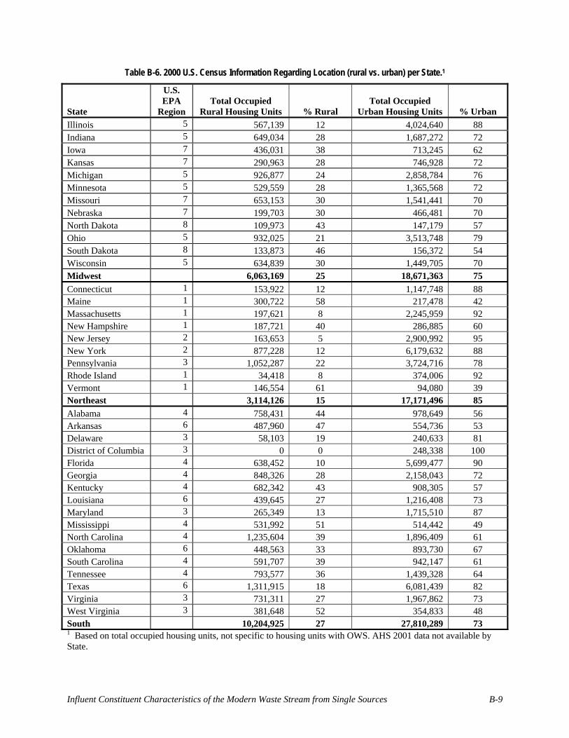
Table B-6. 2000 U.S. Census Information Regarding Location (rural vs. urban) per State.1
State
U.S. EPA
Region Total Occupied
Rural Housing Units % Rural Total Occupied
Urban Housing Units % Urban Illinois 5 567,139 12 4,024,640 88 Indiana 5 649,034 28 1,687,272 72 Iowa 7 436,031 38 713,245 62 Kansas 7 290,963 28 746,928 72 Michigan 5 926,877 24 2,858,784 76 Minnesota 5 529,559 28 1,365,568 72 Missouri 7 653,153 30 1,541,441 70 Nebraska 7 199,703 30 466,481 70 North Dakota 8 109,973 43 147,179 57 Ohio 5 932,025 21 3,513,748 79 South Dakota 8 133,873 46 156,372 54 Wisconsin 5 634,839 30 1,449,705 70 Midwest 6,063,169 25 18,671,363 75 Connecticut 1 153,922 12 1,147,748 88 Maine 1 300,722 58 217,478 42 Massachusetts 1 197,621 8 2,245,959 92 New Hampshire 1 187,721 40 286,885 60 New Jersey 2 163,653 5 2,900,992 95 New York 2 877,228 12 6,179,632 88 Pennsylvania 3 1,052,287 22 3,724,716 78 Rhode Island 1 34,418 8 374,006 92 Vermont 1 146,554 61 94,080 39 Northeast 3,114,126 15 17,171,496 85 Alabama 4 758,431 44 978,649 56 Arkansas 6 487,960 47 554,736 53 Delaware 3 58,103 19 240,633 81 District of Columbia 3 0 0 248,338 100 Florida 4 638,452 10 5,699,477 90 Georgia 4 848,326 28 2,158,043 72 Kentucky 4 682,342 43 908,305 57 Louisiana 6 439,645 27 1,216,408 73 Maryland 3 265,349 13 1,715,510 87 Mississippi 4 531,992 51 514,442 49 North Carolina 4 1,235,604 39 1,896,409 61 Oklahoma 6 448,563 33 893,730 67 South Carolina 4 591,707 39 942,147 61 Tennessee 4 793,577 36 1,439,328 64 Texas 6 1,311,915 18 6,081,439 82 Virginia 3 731,311 27 1,967,862 73 West Virginia 3 381,648 52 354,833 48 South 10,204,925 27 27,810,289 73 1 Based on total occupied housing units, not specific to housing units with OWS. AHS 2001 data not available by State.
Influent Constituent Characteristics of the Modern Waste Stream from Single Sources B-9

Table B-6. 2000 U.S. Census Information Regarding Location (rural vs. urban) per State (continued).1
State
U.S. EPA
Region Total Occupied
Rural Housing Units % Rural Total Occupied
Urban Housing Units % Urban Alaska 10 74,030 33 147,570 67 Arizona 9 211,384 11 1,689,943 89 California 9 670,260 6 10,832,610 94 Colorado 8 251,101 15 1,407,137 85 Hawaii 9 36,269 9 366,971 91 Idaho 10 153,401 33 316,244 67 Montana 8 158,129 44 200,538 56 Nevada 9 62,507 8 688,658 92 New Mexico 6 159,010 23 518,961 77 Oregon 10 275,053 21 1,058,670 79 Utah 8 81,315 12 619,966 88 Washington 10 387,424 17 1,883,974 83 Wyoming 8 64,875 34 128,733 66 West 2,584,758 12 19,859,975 88 United States 21,966,978 21 83,513,123 79 1 Based on total occupied housing units, not specific to housing units with OWS. AHS 2001 data not available by State.
Table B-7. U.S. Census 2004 Poverty Data.1
State
U.S. EPA
Region Population
Number of Individuals Living
Below Poverty Level
Percent of Population Living Below Poverty
Level Illinois 5 12,712,016 1,512,730 11.9Indiana 5 6,226,537 672,466 10.8Iowa 7 2,952,904 292,337 9.9Kansas 7 2,733,697 287,038 10.5Michigan 5 10,104,206 1,242,817 12.3Minnesota 5 5,096,546 423,013 8.3Missouri 7 5,759,532 679,625 11.8Nebraska 7 1,747,704 192,247 11.0North Dakota 8 636,308 76,993 12.1Ohio 5 11,450,143 1,431,268 12.5South Dakota 8 770,621 84,768 11.0Wisconsin 5 5,503,533 588,878 10.7Midwest 65,693,747 7,484,182 11.4
1 Based on total population. Does not reflect the total number of households, occupied households or number of households with OWS.
B -10

Table B-7. U.S. Census 2004 Poverty Data (continued).1
State
U.S. EPA
Region Estimated Population
Number of Individuals Living
Below Poverty Level
Percent of Population Living Below Poverty
Level Connecticut 1 3,498,966 265,921 7.6Maine 1 1,314,985 161,743 12.3Massachusetts 1 6,407,382 589,479 9.2New Hampshire 1 1,299,169 98,737 7.6New Jersey 2 8,685,166 738,239 8.5New York 2 19,280,727 2,737,863 14.2Pennsylvania 3 12,394,471 1,450,153 11.7Rhode Island 1 1,079,916 138,229 12.8Vermont 1 621,233 55,911 9.0Northeast 54,582,015 6,236,276 11.4Alabama 4 4,525,375 728,585 16.1Arkansas 6 2,750,000 492,250 17.9Delaware 3 830,069 82,177 9.9District of Columbia 3 554,239 104,751 18.9Florida 4 17,385,430 2,121,022 12.2Georgia 4 8,918,129 1,319,883 14.8Kentucky 4 4,141,835 720,679 17.4Louisiana 6 4,506,685 874,297 19.4Maryland 3 5,561,332 489,397 8.8Mississippi 4 2,900,768 626,566 21.6North Carolina 4 8,540,468 1,298,151 15.2Oklahoma 6 3,523,546 539,103 15.3South Carolina 4 4,197,892 659,069 15.7Tennessee 4 5,893,298 854,528 14.5Texas 6 22,471,549 3,730,277 16.6Virginia 3 7,481,332 710,727 9.5West Virginia 3 1,812,548 324,446 17.9South 105,994,495 15,675,909 14.8Alaska 10 657,755 53,936 8.2Arizona 9 5,739,879 815,063 14.2California 9 35,842,038 4,766,991 13.3Colorado 8 4,601,821 510,802 11.1Hawaii 9 1,262,124 133,785 10.6Idaho 10 1,395,140 202,295 14.5Montana 8 926,920 131,623 14.2Nevada 9 2,332,898 293,945 12.6New Mexico 6 1,903,006 367,280 19.3Oregon 10 3,591,363 506,382 14.1Utah 8 2,420,708 263,857 10.9Washington 10 6,207,046 813,123 13.1Wyoming 8 505,887 52,106 10.3West 67,386,585 8,911,189 13.2United States 293,656,842 38,307,556 13.0
1 Based on total population. Does not reflect the total number of households, occupied households or number of households with OWS. Influent Constituent Characteristics of the Modern Waste Stream from Single Sources B-111

B.3 National Climatic Data Listings Table B-8. State Average Annual Precipitation and Temperature.
State Average
Precipitation (in.) Average Yearly
Temperature (oF) Midwest
Illinois 37.85 51.95 Indiana 40.16 51.81 Iowa 32.17 47.66 Kansas 27.43 54.25 Michigan 23.98 44.52 Minnesota 26.08 40.77 Missouri 40.92 54.64 Nebraska 22.72 51.24 North Dakota 17.41 39.53 Ohio 38.14 50.72 South Dakota 18.32 44.85 Wisconsin 31.39 43.03
Northeast Connecticut 45.26 48.48 Maine 42.59 41.23 Massachusetts 42.93 47.69 New Hampshire 42.47 43.27 New Jersey 44.87 52.13 New York 39.07 45.24 Pennsylvania 40.02 48.96 Rhode Island 43.32 49.41 Vermont 40.68 42.50
South Alabama 53.90 63.30 Arkansas 49.32 60.72 Delaware 44.52 54.75 Florida 54.11 70.62 Georgia 50.13 63.83 Kentucky 47.53 55.78 Louisiana 57.18 66.59 Maryland 43.08 53.74 Mississippi 55.20 63.83 North Carolina 49.58 59.10 Oklahoma 33.98 59.56 South Carolina 47.96 62.66 Tennessee 52.32 57.95 Texas 28.08 65.06 Virginia 42.76 55.18 West Virginia 44.27 51.91
B -12

Table B-8. State Average Annual Precipitation and Temperature (continued).
State Average
Precipitation (in.) Average Yearly
Temperature (oF) West
Alaska 40.32 32.83 Arizona 12.69 59.85 California 22.27 59.01 Colorado 15.85 44.93 Hawaii 70.00 80.00 Idaho 18.79 44.05 Montana 15.15 42.19 Nevada 8.73 49.32 New Mexico 13.45 53.31 Oregon 26.77 48.16 Utah 11.40 47.99 Washington 37.03 48.04 Wyoming 13.06 41.60
Influent Constituent Characteristics of the Modern Waste Stream from Single Sources B-133

B-144
APPENDIX C
COMPLETE LISTING OF REPORTED BIOCHEMICAL OXYGEN DEMAND (BOD) VALUES
Influent Constituent Characteristics of the Modern Waste Stream from Single Sources C-1

C-2
Tables C-1 through C-12 summarize the reported values and the data qualifiers used. The following key should be used to interpret the data qualifier information within the tables. A more detailed description of the data qualifiers can be found in the report, Section 3.4.1.
Location = state where the study was conducted
Region = location of the study based on US Census defined regions MW = Midwest: IL, IN, IA, KS, MI, MN, MO, NE, ND, OH, SD, and WI NE = Northeast: CT, ME, MA, NH, NJ, NY, PA, RI, VT South: AL, AR, DE, DC, FL, GA, KY, LA, MD, MS, NC, OK, SC, TN, TX, VA, and WV West: AK, AZ, CA, CO, HI, ID, MT, NV, NM, OR, UT, WA, and WY
Lit = literature source 1 – publicly available and published in a peer reviewed journal 2 – publicly available and published in conference proceedings or project report 3 – unpublished; information obtained directly from researcher and is not publicly available
Year = year the study was conducted
Anal = analytical method used 1 – detailed methods used = specified which approved method was used (e.g., APHA 4500-N B). 2 – standard methods = specified use of approved methods (e.g., APHA). 3 – no methods = did not specify which method was used
Type = sampling technique used 1 – composite sample collected 2 – grab sample collected 3 – unknown; type of sample collected was not specified
Freq = frequency of sample collection 1 – at least weekly 2 – bi-weekly to monthly 3 – less than one time per month 4 – unknown
# Events = number of sampling events 1 – more than 12 sampling events reported 2 – between 3 and 12 sampling events reported 3 – less than 3 sampling events reported 4 – unknown; number of sampling events not reported
Season = time of year when study was conducted Spring (Mar-May) Summer (Jun-Aug) Fall (Sept-Nov) Winter (Dec-Feb) All (Jan-Dec)
Data Eval = data evaluation 1 –more than a single average value reported (e.g., descriptive statistics provided) 2 – only the average value reported for each constituent

Table C-1. Reported Single Source Domestic BOD5 Raw Wastewater Values.
BOD5 Location Region Lit Year Anal Type Freq # Events Season Data
Eval Reference
30 Missouri MW 1 2003 3 1 4 4 Spring 2 Dietzman and Gross (2003) 46 Missouri MW 1 2003 3 1 4 4 Spring 2 Dietzman and Gross (2003)
105 Missouri MW 1 2003 3 1 4 4 Spring 2 Dietzman and Gross (2003) 120 Missouri MW 1 2003 3 1 4 4 Spring 2 Dietzman and Gross (2003) 146 1973 3 3 4 4 2 Lawrence (1973) 157 Missouri MW 1 2003 3 1 4 4 Spring 2 Dietzman and Gross (2003) 188 Ontario Canada 1 2004 3 1,2 2 1 All 1 Joy et al. (2004) 207 1973 3 3 4 4 2 Bounds (1997) 241 1973 3 3 4 4 2 Lawrence (1973) 278 Colorado West 1 1974 3 3 4 4 2 Bennett et al. (1974) 284 Kentucky South 1 1967 2 1 4 4 1 Watson et al. (1967) 304 1982 3 3 4 4 2 Bounds (2004) 330 New Mexico West 1 2002 3 1 2 1 All 1 Hanson et al. (2002) 330 1972 3 3 4 4 2 Bounds (1997) 343 Wisconsin MW 1 1974 3 3 4 4 2 Ziebell et al. (1974) 343 1975 3 3 4 4 2 Bounds (1997) 356 Kentucky South 1 1967 2 1 4 4 1 Watson et al. (1967) 415 1975 3 3 4 4 2 Bounds (1997) 435 1971 3 3 4 4 2 Kreissl (1971) 465 1975 3 3 4 4 2 Bounds (1997) 471 Perth Australia 1984 3 3 4 4 1 Troyan et al. (1984) 479 Kentucky South 1 1967 2 1 4 4 1 Watson et al. (1967) 490 1971 3 3 4 4 2 Kreissl (1971) 518 Kentucky South 1 1967 2 1 4 4 1 Watson et al. (1967) 520 1 1976 3 3 4 4 2 Thiruvenkatachari (1976) 523 New Mexico West 1 2002 3 1 2 1 All 1 Hanson et al. (2002) 542 Kentucky South 1 1967 2 1 4 4 1 Watson et al. (1967) 598 Kentucky South 1 1967 2 1 4 4 1 Watson et al. (1967) 1147 New Mexico West 1 2002 3 1 2 1 All 1 Hanson et al. (2002)
blank = information not provided
Influent Constituent Characteristics of the Modern Waste Stream from Single Sources C-3

Table C-2. Reported Multiple Source Domestic BOD5 Raw Wastewater Values.
BOD5 Location Region Lit Year Anal Type Freq # Events Season Data
Eval Reference
144
Michigan, British
Columbia MW,
Canada 2 2002 1 1 4 1 4 Bell and Higgins (2004)
150
Michigan, British
Columbia MW,
Canada 2 2002 1 1 4 1 4 Bell and Higgins (2004) 248 Maine NE 2 1992 3 3 4 2 4 Boyer and Rock (1992) 256 Maine NE 2 1992 3 3 4 2 4 Boyer and Rock (1992) 260 Maine NE 2 1992 3 3 4 2 4 Boyer and Rock (1992) 260 Maine NE 2 1992 3 3 4 2 4 Boyer and Rock (1992) 260 Wisconsin MW 2 1978 2 3 4 1 4 Siegrist (1978) 262 Arizona West 1 1989 2 1 1 2 Fall 1 Anderson and Siegrist (1989) 263 Maine NE 2 1992 3 3 4 2 4 Boyer and Rock (1992) 267 Maine NE 2 1991 3 3 4 2 4 Boyer (1991) 288 Maine NE 2 1991 3 3 4 2 4 Boyer (1991) 307 Maine NE 2 1992 3 3 4 2 4 Boyer and Rock (1992) 580 Arizona West 1 1989 2 1 1 2 Fall 1 Anderson and Siegrist (1989)
blank = information not provided
Table C-3. Reported Food Source BOD5 Raw Wastewater Values.
BOD5 Location Region Lit Year Anal Type Freq # Events Season Data
Eval Reference
1584 Texas South 1 2004 1 2 1 3 Summer 1 Lesikar et al. (2004) 1054 Texas South 1 2004 1 2 1 3 Summer 1 Lesikar et al. (2004) 1045 Texas South 1 2004 1 2 1 3 Summer 1 Lesikar et al. (2004)
blank = information not provided
C-4

Table C-4. Reported Non-medical Source BOD5 Raw Wastewater Values.
BOD5 Location Region Lit Year Anal Type Freq # Events Season Data
Eval Source Type Reference
171 Florida South 1 1998 2 1 2 2 Win –Sum- 1 Min. Security
Correctional Inst. Anderson et al.
(1998)
521 Louisiana South 2 2002 1 3 2 1 All 1 RV Dump/ Rest Area Griffin et al. (2002)
563 Louisiana South 2 2004 3 3 4 4 1 RV Dump/ Rest Area Griffin et al. (2004)
670 California West 2 1987 3 3 4 4 2 Rest Area Pearson et al. (1987)
3080 California West 2 1987 3 3 4 4 2 RV Dump Pearson et al. (1987)
3110 Washington West 2 1987 3 3 4 4 2 RV Dump Kiernan et al. (1987)
blank = information not provided
Table C-5. Reported Single Source Domestic BOD5 STE Values.
BOD5 Location Region Lit Year Anal Type Freq # Events Season Data
Eval Reference
38.5 Ohio MW 1 2002 1 3 3 1 All 2 Steer et al. (2002) 56.8 Ohio MW 1 2002 1 3 3 1 All 2 Steer et al. (2002)
57 Wisconsin MW 1 1977 3 3 4 4 Summer, Fall 1 Sauer and Boyle (1977)
66.9 Ohio MW 1 2002 1 3 3 1 All 2 Steer et al. (2002) 70.9 Ohio MW 1 2002 1 3 3 1 All 2 Steer et al. (2002) 71 Ohio MW 1 2002 1 3 3 1 All 2 Steer et al. (2002)
80.2 Ohio MW 1 2002 1 3 3 1 All 2 Steer et al. (2002) 81 Wisconsin MW 1 1991 3 4 4 1 Tyler et al. (1991) 95 Wisconsin MW 1 1974 2 1 2 2 Summer 1 Otis et al. (1974b)
95.2 Ohio MW 1 2002 1 3 3 1 All 2 Steer et al. (2002) 99.1 Virginia South 1 2001 2 2 4 4 2 Reneau et al. (2001) 101 Ohio MW 1 2002 1 3 3 1 All 2 Steer et al. (2002)
109 Wisconsin MW 1 1977 3 3 4 4 Spring, Summer 1 Sauer and Boyle (1977)
Influent Constituent Characteristics of the Modern Waste Stream from Single Sources C-5

Table C-5. Reported Single Source Domestic BOD5 STE Values (continued).
BOD5 Location Region Lit Year Anal Type Freq # Events Season Data
Eval Reference
109 Virginia South 1 1994 1 3 2 2 Fall - Spring 2 Huang et al. (1994)
111 Wisconsin MW 1 1994 2 2 4 3 1 Converse et al. (1994) 112 Ohio MW 1 2002 1 3 3 1 All 2 Steer et al. (2002)
112 Washington West 2 1981 3 3 2 1 Fall - Spring 1 Seabloom et al. (1981)
112 Ohio MW 1 2002 1 3 3 1 All 2 Steer et al. (2002) 114 N. Carolina South 1 2001 2 3 2 1 All 2 Lindbo and MacConnell (2001)
116 Alabama South 1 1998 2 3 2 2 Summer, Fall 2 O'Driscoll et al. (1998)
116 Virginia South 1 1994 2 3 2 2 Summer, Spring 2 Duncan et al. (1994)
117 Virginia South 1 2001 2 2 4 4 2 Reneau et al. (2001) 118 Ohio MW 1 2002 1 3 3 1 All 2 Steer et al. (2002) 120 1 1976 3 3 4 4 2 Sauer et al. (1976) 120 Minnesota MW 1 2001 2 2 1 1 All 1 Christopherson et al. (2001) 122 Wisconsin MW 1 1974 2 1 2 1 All 1 Otis et al. (1974a)
123 Wisconsin MW 1 1977 3 3 4 4 Fall, Winter 1 Sauer and Boyle (1977)
123 Washington West 2 1981 3 3 2 1 Fall - Spring 1 Seabloom et al. (1981)
123 Washington West 2 1981 3 3 2 1 Fall - Spring 1 Seabloom et al. (1981)
125 Oregon West 1 1982 2 3 4 4 1 Ronayne et al. (1982) 125 Oregon West 1 1994 3 3 1 1 All 2 Ball (1994) 127 Ohio MW 1 1984 2 1 1 1 All 1 Effert et al. (1984) 127 Wisconsin MW 1 1974 2 1 2 1 All 1 Otis et al. (1974a) 128 Alabama South 1 1998 3 3 4 4 1 White and Shirk (1998)
130 Washington West 2 1978 1 3 2 1 Summer, Fall 1 Engeset and Seabloom (1978)
131 Wisconsin MW 1 1974 2 1 2 1 All 1 Otis et al. (1974a) 134 Iowa MW 1 1974 3 2 1 2 2 Karikari et al. (1974)
C-6

Table C-5. Reported Single Source Domestic BOD5 STE Values (continued).
BOD5 Location Region Lit Year Anal Type Freq # Events Season Data
Eval Reference
135 Wisconsin MW 1 1987 2 1 4 4 All 1 Siegrist and Boyle (1987) 136 Ohio MW 1 2002 1 3 3 1 All 2 Steer et al. (2002) 140 Ohio MW 1 2002 1 3 3 1 All 2 Steer et al. (2002) 140 Wisconsin MW 1 1974 2 1 2 2 Summer 1 Otis et al. (1974b)
141 Florida South 1 1991 2 2 1 1 Fall, - Spring 1 Sherman and Anderson (1991)
149 Ohio MW 1 2002 1 3 3 1 All 2 Steer et al. (2002) 149 Oregon West 1 1982 2 3 4 4 1 Ronayne et al. (1982) 150 Ohio MW 1 2002 1 3 3 1 All 2 Steer et al. (2002) 151 New Mexico West 1 2002 3 1 2 1 All 1 Hanson et al. (2002) 153 Wisconsin MW 1 1981 2 1 4 4 1 Hargett et al. (1981) 158 Wisconsin MW 1 1974 3 3 4 4 2 Ziebell et al. (1974) 158 1 1976 3 3 4 4 2 Otis and Boyle (1976)
160.2 Ohio MW 1 2002 1 3 3 1 All 2 Steer et al. (2002) 160.6 Ohio MW 1 2002 1 3 3 1 All 2 Steer et al. (2002) 161 Ohio MW 1 2002 1 3 3 1 All 2 Steer et al. (2002) 162 Montreal Canada 1 1998 3 3 2 1 All 2 Roy et al. (1998) 164 Indiana MW 1 1984 2 3 4 4 1 Hampton and Jones (1984)
166 Washington West 2 1981 3 3 2 1 Fall, - Spring 1 Seabloom et al. (1981)
170 Wisconsin MW 1 1991 3 4 4 1 Tyler et al. (1991) 172 N. Carolina South 1 2001 2 3 2 1 All 2 Lindbo and MacConnell (2001) 174 Indiana MW 1 1984 2 3 4 4 1 Hampton and Jones (1984) 175 Minnesota MW 1 2001 2 2 1 1 All 1 Christopherson et al. (2001) 176 Wisconsin MW 1 1974 2 1 2 1 ALL 1 Otis et al. (1974a) 188 Oregon West 1 1982 2 3 4 4 1 Ronayne et al. (1982) 192 Kentucky South 1 1998 2 3 2 1 All 1 Thom et al. (1998)
192 Wisconsin MW 2 1999 1 2 4 2 Win, - Sum 1 Converse and Converse (1999)
Influent Constituent Characteristics of the Modern Waste Stream from Single Sources C-7

Table C-5. Reported Single Source Domestic BOD5 STE Values (continued).
BOD5 Location Region Lit Year Anal Type Freq # Events Season Data
Eval Reference
193 Wisconsin MW 1 1998 1 2 4 2 Winter -Summer 1 Thom et al. (1998)
193 Ohio MW 1 2002 1 3 3 1 All 2 Steer et al. (2002) 197 Oregon West 1 1982 2 3 4 4 1 Ronayne et al. (1982) 202 Rhode Island NE 2 1999 2 2 2 1 Summer 2 Sykes et al. (1999) 215 Wisconsin MW 1 1998 1 2 4 1 Converse and Converse (1998) 217 Florida South 1 1995 2 2 3 1 All 1 Nielsen et al. (2002) 222 Saskatch. Canada 1 1991 2 2 4 4 1 Viraraghavan and Rana (1991) 222 Oregon West 1 1982 2 3 4 4 1 Ronayne et al. (1982) 224 Oregon West 1 1998 2 3 4 4 1 Thom et al. (1998) 226 Rhode Island NE 2 1999 2 2 2 1 Summer 2 Sykes et al. (1999) 240 Perth Australia 1 1984 3 3 4 4 1 Troyan et al. (1984)
241 Washington West 2 1981 3 3 2 1 Fall, - Spring 1 Seabloom et al. (1981)
245 Maine, Ontario
NE, Canada 1 1994 3 2 2 1 All 1 McKee and Brooks (1994)
246 Rhode Island NE 2 1999 2 2 2 1 Winter 2 Sykes et al. (1999) 249 Rhode Island NE 2 1999 2 2 2 1 winter 2 Sykes et al. (1999)
251 Maine, Ontario
NE, Canada 1 1994 3 2 2 1 All 1 McKee and Brooks (1994)
251 Maine, Ontario
NE, Canada 1 1994 3 2 2 1 All 1 McKee and Brooks (1994)
259 Oregon West 2 2003 2 3 4 3 1 Rich et al. (2003) 260 3 1977 3 3 4 4 2 Siegrist (1977) 261 Oregon West 3 2005 2 2 2,3 1 All 1 Rich (2006) 270 Oregon West 2 2003 2 3 4 3 1 Rich et al. (2003) 280 1 1976 3 3 4 4 2 Thiruvenkatachari (1976) 297 Rhode Island NE 1 2001 2 3 2 2 All 1 Bohrer and Converse (2001) 297 Missouri MW 1 1998 2 3 2 1 All 2 Sievers (1998) 298 Rhode Island NE 2 1999 2 2 2 1 Summer 2 Sykes et al. (1999) 299 Rhode Island NE 2 2002 2 3 2 3 All 1 Loomis et al. (2002)
C-8

Table C-5. Reported Single Source Domestic BOD5 STE Values (continued).
BOD5 Location Region Lit Year Anal Type Freq # Events Season Data
Eval Reference
300 Maryland South 1 1994 3 3 1 1 Fall, Winter 2 Bruen and Piluk (1994)
322 Oregon West 1 1982 2 3 4 4 1 Ronayne et al. (1982)
331 Alabama South 1 1998 2 3 2 2 Summer, Fall 2 O'Driscoll et al. (1998)
348 Oregon West 1 1982 2 3 4 4 1 Ronayne et al. (1982) 351 Rhode Island NE 2 1999 2 2 2 1 Winter 2 Sykes et al. (1999) 378 Oregon West 1 1982 2 3 4 4 1 Ronayne et al. (1982) 861 California West 1980 3 3 4 2 Winter 2 Baker (1980)
blank = information not provided
Table C-6. Reported Multiple Source Domestic BOD5 STE Values.
BOD5 Location Region Lit Year Anal Type Freq # Events Season Data
Eval Reference
63 Minnesota MW 1 2001 2 3 2 1 All 1 Henneck et al. (2001) 95 New Mexico West 1 1991 3 2 4 4 1 Jacquez et al. (1991)
122 Ontario Canada 1 1974 3 3 1 1 All 2 Brandes et al. (1974) 145 Maine NE 2 1992 3 3 4 4 2 Boyer and Rock (1992) 150 Wisconsin MW 2 1991 3 2 4 4 1 Converse et al. (1991) 168 Wisconsin MW 1 1983 2 2 3 2 All 2 Siegrist et al. (1985) 177 Maine NE 2 1992 3 3 4 4 2 Boyer and Rock (1992) 179 W. Virginia South 1 1991 2 3 1 4 2 Sack et al. (1991) 184 Minnesota MW 1 2001 2 3 2 1 All 1 Henneck et al. (2001) 184 Maine NE 2 1991 3 3 4 4 2 Boyer (1991) 185 Norway Norway 1 1991 2 3 1 2 1 Siegrist et al. (1991) 188 Maine NE 2 1992 3 3 4 4 2 Boyer and Rock (1992) 191 Maine NE 2 1992 3 3 4 4 2 Boyer and Rock (1992) 195 Maine NE 2 1992 3 3 4 4 2 Boyer and Rock (1992) 195 Maine NE 2 1991 3 3 4 4 2 Boyer (1991) 219 1985 3 3 4 4 2 Swed (1985) 229 Maine NE 2 1992 3 3 4 4 2 Boyer and Rock (1992)
blank = information not provided
Influent Constituent Characteristics of the Modern Waste Stream from Single Sources C-9

Table C-7. Reported Food Source BOD5 STE Values.
BOD5 Location Region Lit Year Anal Type Freq # Events Season Data
Eval Reference
74.2 Mass. NE 2 1999 2 2 3 2 All 1 Higgins and Groves (1999) 159 Florida South 3 1995 1 2 4 3 2 Bloomquist and Schmidt (1995) 162 Florida South 3 1995 1 2 4 3 2 Bloomquist and Schmidt (1995) 179 Wisconsin MW 1 1984 2 2 4 4 2 Siegrist et al. (1984b) 228 Florida South 3 1995 1 2 4 3 2 Bloomquist and Schmidt (1995) 245 Wisconsin MW 1 1984 2 2 4 4 2 Siegrist et al. (1984b) 261 Wisconsin MW 1 1984 2 2 4 4 2 Siegrist et al. (1984b) 270 Florida South 3 1995 1 2 4 3 2 Bloomquist and Schmidt (1995) 278 Florida South 3 1995 1 2 4 3 2 Bloomquist and Schmidt (1995) 335 Florida South 3 1995 1 2 4 3 2 Bloomquist and Schmidt (1995) 377 Wisconsin MW 1 1984 2 2 4 4 2 Siegrist et al. (1984b) 401 Florida South 3 1995 1 2 4 3 2 Bloomquist and Schmidt (1995) 410 Mass. NE 2 1999 2 2 3 2 All 1 Higgins and Groves (1999) 420 Florida South 3 1995 1 2 4 3 2 Bloomquist and Schmidt (1995) 465 Florida South 3 1995 1 2 4 3 2 Bloomquist and Schmidt (1995)
493 Maine, Ontario
NE, Canada 1 1994 3 2 2 1 All 1 McKee and Brooks (1994)
501 Florida South 3 1995 1 2 4 3 2 Bloomquist and Schmidt (1995) 510 Florida South 3 1995 1 2 4 3 2 Bloomquist and Schmidt (1995) 510 Florida South 3 1995 1 2 4 3 2 Bloomquist and Schmidt (1995) 525 Florida South 3 1995 1 2 4 3 2 Bloomquist and Schmidt (1995) 540 Florida South 3 1995 1 2 4 3 2 Bloomquist and Schmidt (1995) 582 Wisconsin MW 1 1984 2 2 4 4 2 Siegrist et al. (1984b) 588 Florida South 3 1995 1 2 4 3 2 Bloomquist and Schmidt (1995) 593 Florida South 3 1995 1 2 4 3 2 Bloomquist and Schmidt (1995) 600 Florida South 3 1995 1 2 4 3 2 Bloomquist and Schmidt (1995) 615 Florida South 3 1995 1 2 4 3 2 Bloomquist and Schmidt (1995) 690 Florida South 3 1995 1 2 4 3 2 Bloomquist and Schmidt (1995) 693 Wisconsin MW 1 1984 2 2 4 4 2 Siegrist et al. (1984b)
C-10

Table C-7. Reported Food Source BOD5 STE Values (continued).
BOD5 Location Region Lit Year Anal Type Freq # Events Season Data
Eval Reference
693 Florida South 3 1995 1 2 4 3 2 Bloomquist and Schmidt (1995) 720 Florida South 3 1995 1 2 4 3 2 Bloomquist and Schmidt (1995) 720 Florida South 3 1995 1 2 4 3 2 Bloomquist and Schmidt (1995) 762 Florida South 3 1995 1 2 4 3 2 Bloomquist and Schmidt (1995) 780 Florida South 3 1995 1 2 4 3 2 Bloomquist and Schmidt (1995) 792 Mass. NE 2 1999 2 2 3 2 All 1 Higgins and Groves (1999) 843 Florida South 3 1995 1 2 4 3 2 Bloomquist and Schmidt (1995) 880 Wisconsin MW 1 1984 2 2 4 4 2 Siegrist et al. (1984b) 891 Florida South 3 1995 1 2 4 3 2 Bloomquist and Schmidt (1995)
1068 Florida South 3 1995 1 2 4 3 2 Bloomquist and Schmidt (1995) 1095 Florida South 3 1995 1 2 4 3 2 Bloomquist and Schmidt (1995) 1140 Florida South 3 1995 1 2 4 3 2 Bloomquist and Schmidt (1995) 1140 Florida South 3 1995 1 2 4 3 2 Bloomquist and Schmidt (1995) 2820 Florida South 3 1995 1 2 4 3 2 Bloomquist and Schmidt (1995)
>1020 Florida South 3 1995 1 2 4 3 2 Bloomquist and Schmidt (1995) >1020 Florida South 3 1995 1 2 4 3 2 Bloomquist and Schmidt (1995)
blank = information not provided
Table C-8. Reported Non-medical Source BOD5 STE Values.
BOD5 Location Region Lit Year Anal Type Freq # Events Season Data Eval Source Type Reference
28 Maine, Ontario
NE, Canada 1 1994 3 2 2 1 All 1 School McKee and Brooks
(1994)
29 Maine, Ontario
NE, Canada 1 1994 3 2 2 1 All 1 School McKee and Brooks
(1994)
37 Maine, Ontario
NE, Canada 1 1994 3 2 2 1 All 1 School McKee and Brooks
(1994)
46 Mass. NE 2 1999 2 2 3 2 All 1 School Higgins and Groves (1999)
53.6 Oregon West 1 1982 2 3 4 4 1 Sawmill Ronayne et al. (1982)
Influent Constituent Characteristics of the Modern Waste Stream from Single Sources C-11

Table C-8. Reported Non-medical Source BOD5 STE Values (continued).
BOD5 Location Region Lit Year Anal Type Freq # Events Season Data Eval Source Type Reference
65 Maine, Ontario
NE, Canada 1 1994 3 2 2 1 All 1 Shopping Plaza McKee and Brooks
(1994)
71 Maine, Ontario
NE, Canada 1 1994 3 2 2 1 All 1 School McKee and Brooks
(1994)
78.6 Mass. NE 2 1999 2 2 3 2 All 1 School Higgins and Groves (1999)
81 Maine, Ontario
NE, Canada 1 1994 3 2 2 1 All 1 School McKee and Brooks
(1994)
93.5 Florida South 1 1993 2 1 3 2 All 1 Campus Christian Center & Dorm
Anderson et al. (1994)
95.5 Mass. NE 2 1999 2 2 3 2 All 1 School Higgins and Groves (1999)
97 Virginia South 2 2002 3 3 4 4 2 One room
schoolhouse turned into museum
Hatch et al. (2002)
97.2 Mass. NE 2 1999 2 2 3 2 All 1 School Higgins and Groves (1999)
101 Mass. NE 2 1999 2 2 3 2 All 1 School Higgins and Groves (1999)
101 Wisconsin MW 1 1984 2 2 4 4 2 Golf club Siegrist et al. (1984b)105 New Mexico West 2 2002 3 3 4 4 2 School Egemen et al. (2002)
107 Mass. NE 2 1999 2 2 3 2 All 1 School Higgins and Groves (1999)
118 Tennessee South 3 2003 1 2 3 3 Summer 2 Marina Matassa et al. (2003)130 Tennessee South 3 2003 1 2 3 3 Summer 2 Marina Matassa et al. (2003)
137 Mass. NE 2 1999 2 2 3 2 All 1 Office Higgins and Groves (1999)
158 Mass. NE 2 1999 2 2 3 2 All 1 School Higgins and Groves (1999)
161 Oregon West 1 1982 2 3 4 4 1 Office Ronayne et al. (1982)171 Wisconsin MW 1 1984 2 2 4 4 2 Motel Siegrist et al. (1984b)187 California West 2 1980 3 3 4 2 Winter 2 Ski area Baker (1980)
193 Wisconsin MW 1 1994 2 1 2 1 All 1 Correctional institution Boyle et al. (1994)
197 Wisconsin MW 1 1984 2 2 4 4 2 Golf club Siegrist et al. (1984b)
C-12

Table C-8. Reported Non-medical Source BOD5 STE Values (continued).
BOD5 Location Region Lit Year Anal Type Freq # Events Season Data Eval Source Type Reference
207 Oregon, Arizona West 2 1999 3 3 4 4 2 Convenience Store Ball et al. (1999)
209 Minnesota MW 2 1999 2 3 2 1 Winter -Summer 1 Correctional
Facility McCarthy et al.
(1999)
224 Minnesota MW 2 1999 2 3 2 1 Winter -Summer 1 Correctional
Facility McCarthy et al.
(1999)
244 Minnesota MW 2 1999 2 3 2 1 Winter -Summer 1 Correctional
Facility McCarthy et al.
(1999)
248 Minnesota MW 2 1999 2 3 2 1 Winter -Summer 1 Correctional
Facility McCarthy et al.
(1999)
248 Minnesota MW 2 1999 2 3 2 1 Winter -Summer 1 Correctional
Facility McCarthy et al.
(1999)
250 Minnesota MW 2 1999 2 3 2 1 Winter -Summer 1 Correctional
Facility McCarthy et al.
(1999)
253 Minnesota MW 2 1999 2 3 2 1 Winter -Summer 1 Correctional
Facility McCarthy et al.
(1999)
255 Minnesota MW 2 1999 2 3 2 1 Winter -Summer 1 Correctional
Facility McCarthy et al.
(1999) 255 Tennessee South 3 2003 1 2 3 3 Summer 2 Marina Matassa et al. (2003)
257 Minnesota MW 2 1999 2 3 2 1 Winter -Summer 1 Correctional
Facility McCarthy et al.
(1999)
266 Minnesota MW 1 2001 2 3 2 1 All 1 Correctional Facility Henneck et al. (2001)
276.8 Mass. NE 2 1999 2 2 3 2 All 1 Office Higgins and Groves (1999)
278 Minnesota MW 2 1999 2 3 2 1 Winter -Summer 1 Correctional
Facility McCarthy et al.
(1999)
280 Mass. NE 2 1999 2 2 3 2 All 1 Office Higgins and Groves (1999)
286 Minnesota MW 2 1999 2 3 2 1 Winter -Summer 1 Correctional
Facility McCarthy et al.
(1999)
302 Minnesota MW 2 1999 2 3 2 1 Winter -Summer 1 Correctional
Facility McCarthy et al.
(1999)
308 Minnesota MW 2 1999 2 3 2 1 Winter -Summer 1 Correctional
Facility McCarthy et al.
(1999)
Influent Constituent Characteristics of the Modern Waste Stream from Single Sources C-13

Table C-8. Reported Non-medical Source BOD5 STE Values (continued).
BOD5 Location Region Lit Year Anal Type Freq # Events Season Data Eval Source Type Reference
309 Minnesota MW 2 1999 2 3 2 1 Winter -Summer 1 Correctional
Facility McCarthy et al.
(1999)
310 Minnesota MW 2 1999 2 3 2 1 Winter -Summer 1 Correctional
Facility McCarthy et al.
(1999)
310 Minnesota MW 2 1999 2 3 2 1 Winter -Summer 1 Correctional
Facility McCarthy et al.
(1999)
314 Minnesota MW 2 1999 2 3 2 1 Winter -Summer 1 Correctional
Facility McCarthy et al.
(1999) 326 Tennessee South 3 2003 1 2 3 3 Summer 2 Marina Matassa et al. (2003)333 Wisconsin MW 1 1984 2 2 4 4 2 Golf club Siegrist et al. (1984b)377 Tennessee South 3 2003 1 2 3 3 Summer 2 Campground Matassa et al. (2003)395 Tennessee South 3 2003 1 2 3 3 Summer 2 Marina Matassa et al. (2003)406 Tennessee South 3 2003 1 2 3 3 Summer 2 Marina Matassa et al. (2003)644 Tennessee South 3 2003 1 2 3 3 Summer 2 Marina Matassa et al. (2003)657 Tennessee South 3 2003 1 2 3 3 Summer 2 Campground Matassa et al. (2003)901 Tennessee South 3 2003 1 2 3 3 Summer 2 Marina Matassa et al. (2003)1117 Tennessee South 3 2003 1 2 3 3 Summer 2 Campground Matassa et al. (2003)1537 Tennessee South 3 2003 1 2 3 3 Summer 2 Campground Matassa et al. (2003)
blank = information not provided
C-14

Table C-9. Reported Medical Source BOD5 STE Values.
BOD5 Location Region Lit Year Anal Type Freq # Events Season Data
Eval Source Type Reference
104 Mass. NE 2 1999 2 2 3 2 All 1 Doctor Higgins and Groves (1999)
109 Mass. NE 2 1999 2 2 3 2 All 1 Veterinary/ Kennel
Higgins and Groves (1999)
128 Mass. NE 2 1999 2 2 3 2 All 1 Assisted Living Facility
Higgins and Groves (1999)
138 Mass. NE 2 1999 2 2 3 2 All 1 Veterinary/ Kennel
Higgins and Groves (1999)
150 Mass. NE 2 1999 2 2 3 2 All 1 Doctor Higgins and Groves (1999)
169 Mass. NE 2 1999 2 2 3 2 All 1 Nursing Home Higgins and Groves (1999)
224 Mass. NE 2 1999 2 2 3 2 All 1 Assisted Living Facility
Higgins and Groves (1999)
250 Mass. NE 2 1999 2 2 3 2 All 1 Veterinary/ Kennel
Higgins and Groves (1999)
291 Mass. NE 2 1999 2 2 3 2 All 1 Nursing Home Higgins and Groves (1999)
292 Mass. NE 2 1999 2 2 3 2 All 1 Assisted Living Facility
Higgins and Groves (1999)
402 Mass. NE 2 1999 2 2 3 2 All 1 Nursing Home Higgins and Groves (1999)
431 Mass. NE 2 1999 2 2 3 2 All 1 Doctor Higgins and Groves (1999)
blank = information not provided
Influent Constituent Characteristics of the Modern Waste Stream from Single Sources C-15

Table C-10. Reported Municipal Source BOD5 Values.
BOD5 (mg/L) Sample Description Reference 117 Influent Littleton et al. (2003) 135 Influent Yang et al. (2004)
146.4 Raw Wastewater Babcock et al. (2001) 148 Influent Stephens et al. (2004) 156 Influent Sadler et al. (2002) 159 Influent Sadler et al. (2002) 159 Influent Insel et al. (2003)
170.5 Influent Kwon et al. (2003) 172 Influent Littleton et al. (2003) 172 Raw Wastewater Jones and Takacs (2004) 177 Influent Sadler et al. (2002) 178 Influent Rock and Capron (2002) 183 Influent Bradstreet et al. (2002) 186 Influent Stephens et al. (2004) 195 Influent Sadler et al. (2002) 196 Influent Stephens et al. (2004) 199 Influent Stephens et al. (2004) 203 Influent Littleton et al. (2003) 208 Influent Crites et al. (2002) 210 Influent Littleton et al. (2003) 216 Influent Sadler et al. (2002) 220 Influent Chaparro and Noguera (2002) 221 Influent Littleton et al. (2003) 225 Typical Raw Wastewater Lorenz et al. (2002) 237 Influent Littleton et al. (2003) 240 Influent Sauer et al. (2000) 260 Influent Sova et al. (2004) 264 Influent Danielson (2006) 294 Influent Littleton et al. (2003) 300 Typical Wastewater Composition Shechter et al. (2002) 301 Unknown Baumann and Babbitt (1953) 342 Raw Wastewater Crawford et al. (2000) 364 Influent Zheng et al. (2002) 369 Influent Danielson (2006) 554 Influent Zheng et al. (2002)
C-16

Table C-10. Reported Municipal Source BOD5 Values (continued).
BOD5 (mg/L) Sample Description Reference 630 Influent Garcia and Kanj (2002) 797 Raw Wastewater Xingcan et al. (2001) 2650 Wastewater Characteristics Gale (2002)
Table C-11. Other Reported Oxygen Demand Values.
Average Value Constituent (units) Source Waste Stream Reference 164 cBOD5 (mg/L) Raw Single source domestic Joy et al. (2004) 212 cBOD5 (mg/L) Raw Single source domestic Edvardsson (2002) 212 cBOD5 (mg/L) Raw Single source domestic Edvardsson and Spears (2000)
137.8 cBOD5 (mg/L) Raw Non-medical, Min. Security Correctional Inst. Anderson et al. (1998) 160.2 cBOD5 (mg/L) STE Single source domestic Cagle and Johnson (1994) 175 cBOD5 (mg/L) STE Single source domestic Siegrist et al. (2000) 332 cBOD5 (mg/L) STE Single source domestic Siegrist et al. (2000)
150.9 cBOD5 (mg/L) STE Non-medical, Camp Whitehill et al. (2003) 167.3 cBOD5 (mg/L) STE Non-medical, Residential/Health Clinic/Casino Martinson et al. (2001) 223 cBOD5 (mg/L) STE Non-medical, Restaurant Bloomquist and Schmidt (1995) 341 cBOD5 (mg/L) STE Non-medical, Restaurant Bloomquist and Schmidt (1995) 345 cBOD5 (mg/L) STE Non-medical, Restaurant Bloomquist and Schmidt (1995) 382 cBOD5 (mg/L) STE Non-medical, Restaurant Bloomquist and Schmidt (1995)
387.5 cBOD5 (mg/L) STE Non-medical, Restaurant Bloomquist and Schmidt (1995) 390 cBOD5 (mg/L) STE Non-medical, Restaurant Bloomquist and Schmidt (1995) 413 cBOD5 (mg/L) STE Non-medical, Restaurant Bloomquist and Schmidt (1995) 555 cBOD5 (mg/L) STE Non-medical, Restaurant Bloomquist and Schmidt (1995)
587.5 cBOD5 (mg/L) STE Non-medical, Restaurant Bloomquist and Schmidt (1995) 615 cBOD5 (mg/L) STE Non-medical, Restaurant Bloomquist and Schmidt (1995)
620.5 cBOD5 (mg/L) STE Non-medical, Restaurant Bloomquist and Schmidt (1995) 649.7 cBOD5 (mg/L) STE Non-medical, Grocery Store with Meat Packing Whitehill et al. (2003) 678 cBOD5 (mg/L) STE Non-medical, Restaurant Bloomquist and Schmidt (1995) 684 cBOD5 (mg/L) STE Non-medical, Restaurant Bloomquist and Schmidt (1995) 699 cBOD5 (mg/L) STE Non-medical, Restaurant Bloomquist and Schmidt (1995) 780 cBOD5 (mg/L) STE Non-medical, Restaurant Bloomquist and Schmidt (1995)
1030.5 cBOD5 (mg/L) STE Non-medical, Restaurant Bloomquist and Schmidt (1995)
Influent Constituent Characteristics of the Modern Waste Stream from Single Sources C-177

Table C-11. Other Reported Oxygen Demand Values (continued).
Average Value Constituent (units) Source Waste Stream Reference 1440 cBOD5 (mg/L) STE Non-medical, Restaurant Bloomquist and Schmidt (1995) 2466 cBOD5 (mg/L) STE Non-medical, Restaurant Bloomquist and Schmidt (1995) 540 COD (mg/L) Raw Single source domestic Watson et al. (1967) 640 COD (mg/L) Raw Single source domestic Watson et al. (1967) 705 COD (mg/L) Raw Single source domestic Watson et al. (1967) 727 COD (mg/L) Raw Single source domestic Edvardsson and Spears (2000) 882 COD (mg/L) Raw Single source domestic Watson et al. (1967) 905 COD (mg/L) Raw Single source domestic Bennett et al. (1974)
914.1 COD (mg/L) Raw Single source domestic Hanson et al. (2002) 959 COD (mg/L) Raw Single source domestic Watson et al. (1967) 1000 COD (mg/L) Raw Single source domestic Thiruvenkatachari (1976) 1133 COD (mg/L) Raw Single source domestic Watson et al. (1967) 1842 COD (mg/L) Raw Single source domestic Hanson et al. (2002)
2404.2 COD (mg/L) Raw Single source domestic Hanson et al. (2002) 730 COD (mg/L) Raw Non-medical, Lab (simulated household) Siegrist (1978) 1756 COD (mg/L) Raw Non-medical, Rest Area Restroom Pearson et al. (1987) 6209 COD (mg/L) Raw Non-medical, RV Dump Pearson et al. (1987) 8230 COD (mg/L) Raw Non-medical, RV Dump Kiernan et al. (1987) 157 COD (mg/L) STE Single source domestic Tyler et al. (1991) 189 COD (mg/L) STE Single source domestic Seabloom et al. (1981) 220 COD (mg/L) STE Single source domestic Otis et al. (1974b) 228 COD (mg/L) STE Single source domestic Converse et al. (1994) 251 COD (mg/L) STE Single source domestic Seabloom et al. (1981) 260 COD (mg/L) STE Single source domestic Siegrist et al. (2000) 265 COD (mg/L) STE Single source domestic Hargett et al. (1981) 265 COD (mg/L) STE Single source domestic Seabloom et al. (1981) 266 COD (mg/L) STE Single source domestic Engeset and Seabloom (1978) 289 COD (mg/L) STE Single source domestic Sauer et al. (1976) 291 COD (mg/L) STE Single source domestic Otis et al. (1974a) 310 COD (mg/L) STE Single source domestic Effert et al. (1984) 312 COD (mg/L) STE Single source domestic Jacquez et al. (1991) 312 COD (mg/L) STE Single source domestic Hampton and Jones (1984)
C-18

Table C-11. Other Reported Oxygen Demand Values (continued).
Average Value Constituent (units) Source Waste Stream Reference 315 COD (mg/L) STE Single source domestic Roy et al. (1998) 323 COD (mg/L) STE Single source domestic Hampton and Jones (1984) 325 COD (mg/L) STE Single source domestic Otis et al. (1974a) 335 COD (mg/L) STE Single source domestic Otis et al. (1974b) 337 COD (mg/L) STE Single source domestic Otis et al. (1974a) 351 COD (mg/L) STE Single source domestic Siegrist and Boyle (1987) 360 COD (mg/L) STE Single source domestic Otis and Boyle (1976) 361 COD (mg/L) STE Single source domestic Otis et al. (1974a)
380.9 COD (mg/L) STE Single source domestic Viraraghavan and Rana (1991) 397 COD (mg/L) STE Single source domestic Karikari et al. (1974)
421.8 COD (mg/L) STE Single source domestic Hanson et al. (2002) 458 COD (mg/L) STE Single source domestic Converse and Converse (1999) 461 COD (mg/L) STE Single source domestic Converse and Converse (1998) 486 COD (mg/L) STE Single source domestic Seabloom et al. (1981) 496 COD (mg/L) STE Single source domestic Siegrist et al. (2000) 550 COD (mg/L) STE Single source domestic Thiruvenkatachari (1976) 568 COD (mg/L) STE Single source domestic Viraraghavan and Warnock (1974) 630 COD (mg/L) STE Single source domestic Rock et al. (1981) 710 COD (mg/L) STE Single source domestic Seabloom et al. (1981) 1931 COD (mg/L) STE Single source domestic Baker (1980) 170 COD (mg/L) STE Multiple source domestic Jacquez et al. (1991) 233 COD (mg/L) STE Multiple source domestic Brandes et al. (1974) 291 COD (mg/L) STE Multiple source domestic Converse et al. (1991) 169 COD (mg/L) STE Non-medical, Lab (simulated household) Siegrist (1978) 227 COD (mg/L) STE Non-medical, Golf Club Siegrist et al. (1984b) 228 COD (mg/L) STE Non-medical, Residential/ Church/ School Siegrist et al. (1984a) 268 COD (mg/L) STE Non-medical, Residential/ Church/ School Siegrist et al. (1984a) 276 COD (mg/L) STE Non-medical, Residential/ Church/ School Siegrist et al. (1984a) 284 COD (mg/L) STE Non-medical, Residential/ Church/ School Siegrist et al. (1984a) 338 COD (mg/L) STE Non-medical, Residential/ Church/ School Siegrist et al. (1984a) 347 COD (mg/L) STE Non-medical, Research Center Roy et al. (1998) 381 COD (mg/L) STE Non-medical, Motel Siegrist et al. (1984b)
Influent Constituent Characteristics of the Modern Waste Stream from Single Sources C-19

Table C-11. Other Reported Oxygen Demand Values (continued).
Average Value Constituent (units) Source Waste Stream Reference 416 COD (mg/L) STE Non-medical, Golf Club Siegrist et al. (1984b) 449 COD (mg/L) STE Non-medical, Bar/Grill Siegrist et al. (1984b) 586 COD (mg/L) STE Non-medical, Restaurant Siegrist et al. (1984b) 620 COD (mg/L) STE Non-medical, Golf Club Siegrist et al. (1984b) 622 COD (mg/L) STE Non-medical, Restaurant Siegrist et al. (1984b) 690 COD (mg/L) STE Non-medical, Dairy Farm Christopherson et al. (2004) 772 COD (mg/L) STE Non-medical, Restaurant Siegrist et al. (1984b) 1116 COD (mg/L) STE Non-medical, Dairy Farm Christopherson et al. (2004) 1196 COD (mg/L) STE Non-medical, Restaurant Siegrist et al. (1984b) 1321 COD (mg/L) STE Non-medical, Restaurant Siegrist et al. (1984b) 1667 COD (mg/L) STE Non-medical, Restaurant Siegrist et al. (1984b) 1930 COD (mg/L) STE Non-medical, Dairy Farm Christopherson et al. (2004) 4122 COD (mg/L) STE Non-medical, Dairy Farm Christopherson et al. (2004) 5080 COD (mg/L) STE Non-medical, Dairy Farm Christopherson et al. (2004)
C-20

Table C-12. Other Reported Carbon Values.
Average Value Constituent (units) Source Waste Stream Reference 90.3 DIC (mg/L) STE Single source domestic Wilhelm et al. (1996) 102 DIC (mg/L) STE Single source domestic Wilhelm et al. (1996) 31.8 DOC (mg/l) STE Non-medical, Campground Ptacek (1998) 38.2 DOC (mg/l) STE Single source domestic Wilhelm et al. (1996) 71.3 DOC (mg/l) STE Single source domestic Wilhelm et al. (1996) 94 DOC (mg/l) STE Single source domestic Robertson and Blowes (1995)
121 TOC (mg/L) Raw Single source domestic Edvardsson and Spears (2000) 91 TOC (mg/L) STE Multiple source domestic Siegrist et al. (1991)
94.9 TOC (mg/L) STE Multiple source domestic Brown et al. (1977) 86 TOC (mg/L) STE Non-medical, Correctional Institution Boyle et al. (1994) 41 TOC (mg/L) STE Single source domestic Tyler et al. (1991)
47.4 TOC (mg/L) STE Campus Christian Center & Dorm Anderson et al. (1994) 58.6 TOC (mg/L) STE Single source domestic Wolf et al. (1998) 61 TOC (mg/L) STE Single source domestic Converse et al. (1994)
69.2 TOC (mg/L) STE Single source domestic Viraraghavan and Rana (1991) 72.8 TOC (mg/L) STE Single source domestic Thom et al. (1998) 73 TOC (mg/L) STE Single source domestic Viraraghavan and Warnock (1974)
83.6 TOC (mg/L) STE Single source domestic Thom et al. (1998) 99 TOC (mg/L) STE Single source domestic Siegrist and Boyle (1987)
106 TOC (mg/L) STE Single source domestic Tyler et al. (1991) 107 TOC (mg/L) STE Single source domestic Converse and Converse (1998) 147 TOC (mg/L) STE Single source domestic Converse and Converse (1999)
Influent Constituent Characteristics of the Modern Waste Stream from Single Sources C-21

C-22

APPENDIX D
COMPLETE LISTING OF REPORTED SOLIDS VALUES
Influent Constituent Characteristics of the Modern Waste Stream from Single Sources D-1

D-2
Tables D-1 through D-11 summarize the reported values and the data qualifiers used. The following key should be used to interpret the data qualifier information within the tables. A more detailed description of the data qualifiers can be found in the report, Section 3.4.1.
Location = state where the study was conducted
Region = location of the study based on US Census defined regions MW = Midwest: IL, IN, IA, KS, MI, MN, MO, NE, ND, OH, SD, and WI NE = Northeast: CT, ME, MA, NH, NJ, NY, PA, RI, VT South: AL, AR, DE, DC, FL, GA, KY, LA, MD, MS, NC, OK, SC, TN, TX, VA, and WV West: AK, AZ, CA, CO, HI, ID, MT, NV, NM, OR, UT, WA, and WY
Lit = literature source 1 – publicly available and published in a peer reviewed journal 2 – publicly available and published in conference proceedings or project report 3 – unpublished; information obtained directly from researcher and is not publicly available
Year = year the study was conducted
Anal = analytical method used 1 – detailed methods used = specified which approved method was used (e.g., APHA 4500-N B). 2 – standard methods = specified use of approved methods (e.g., APHA). 3 – no methods = did not specify which method was used
Type = sampling technique used 1 – composite sample collected 2 – grab sample collected 3 – unknown; type of sample collected was not specified
Freq = frequency of sample collection 1 – at least weekly 2 – bi-weekly to monthly 3 – less than one time per month 4 – unknown
# Events = number of sampling events 1 – more than 12 sampling events reported 2 – between 3 and 12 sampling events reported 3 – less than 3 sampling events reported 4 – unknown; number of sampling events not reported
Season = time of year when study was conducted Spring (Mar-May) Summer (Jun-Aug) Fall (Sept-Nov) Winter (Dec-Feb) All (Jan-Dec)
Data Eval = data evaluation 1 –more than a single average value reported (e.g., descriptive statistics provided) 2 – only the average value reported for each constituent

Table D-1. Reported Single Source Domestic TSS Raw Wastewater Values.
TSS Location Region Lit Year Anal Type Freq # Events Season Data
Eval Reference
18 Missouri MW 1 2003 3 1 4 4 2 Dietzman and Gross (2003) 38 Missouri MW 1 2003 3 1 4 4 2 Dietzman and Gross (2003) 44 Missouri MW 1 2003 3 1 4 4 2 Dietzman and Gross (2003) 60 Missouri MW 1 2003 3 1 4 4 2 Dietzman and Gross (2003) 69 Missouri MW 1 2003 3 1 4 4 2 Dietzman and Gross (2003)
126 1973 3 3 4 4 2 Lawrence (1973) 151 Ontario Canada 1 2004 3 1, 2 2 1 All 1 Joy et al. (2004) 165 1973 3 3 4 4 2 Bounds (1997) 200 1976 3 3 4 4 2 Thiruvenkatachari (1976) 200 1973 3 3 4 4 2 Lawrence (1973) 226 1982 3 3 4 4 2 Bounds (2004) 259 Wisconsin MW 1 1974 3 3 4 4 2 Ziebell et al. (1974) 259 1975 3 3 4 4 2 Bounds (1997) 267 California West 2 2002 3 2 4 2 2 Edvardsson (2002) 267 California West 2 2000 3 1 1 1 Summer 1 Edvardsson and Spears (2000) 293 Kentucky South 1 1967 2 1 4 4 1 Watson et al. (1967) 296 1975 3 3 4 4 2 Bounds (1997) 310 1972 3 3 4 4 2 Bounds (1997) 360 Kentucky South 1 1967 2 1 4 4 1 Watson et al. (1967) 363 Kentucky South 1 1967 2 1 4 4 1 Watson et al. (1967) 380 1971 3 3 4 4 2 Kreissl (1971) 394 1975 3 3 4 4 2 Bounds (1997) 396 Colorado West 1 1974 3 3 4 4 2 Bennett et al. (1974) 473 Kentucky South 1 1967 2 1 4 4 1 Watson et al. (1967) 478 Kentucky South 1 1967 2 1 4 4 1 Watson et al. (1967) 480 1971 3 3 4 4 2 Kreissl (1971) 500 Perth Australia 1984 3 3 4 4 1 Troyan et al. (1984) 602 Kentucky South 1 1967 2 1 4 4 1 Watson et al. (1967)
1295.8 New Mexico West 1 2002 3 1 2 1 All 1 Hanson et al. (2002) 1356.1 New Mexico West 1 2002 3 1 2 1 All 1 Hanson et al. (2002) 2232.6 New Mexico West 1 2002 3 1 2 1 All 1 Hanson et al. (2002)
blank = information not provided
Influent Constituent Characteristics of the Modern Waste Stream from Single Sources D-3

Table D-2. Reported Multiple-Source Domestic TSS Raw Wastewater Values.
TSS Location Region Lit Year Anal Type Freq # Events Season Data
Eval Reference
180 Michigan,
British Columbia
MW, Canada 2 2002 1 1 4 4 1 Bell and Higgins (2004)
196 Maine NE 2 1992 3 3 4 4 2 Boyer and Rock (1992)
197 Michigan,
British Columbia
MW, Canada 2 2002 1 1 4 4 1 Bell and Higgins (2004)
202 Maine NE 2 1992 3 3 4 4 2 Boyer and Rock (1992) 217 Maine NE 2 1992 3 3 4 4 2 Boyer and Rock (1992) 228 Arizona West 1 1989 3 1 1 3 Fall 1 Anderson and Siegrist (1989) 306 Maine NE 2 1991 3 3 4 4 2 Boyer (1991) 310 Maine NE 2 1991 3 3 4 4 2 Boyer (1991) 317 Maine NE 2 1992 3 3 4 4 2 Boyer and Rock (1992) 320 Maine NE 2 1992 3 3 4 4 2 Boyer and Rock (1992) 345 Maine NE 2 1992 3 3 4 4 2 Boyer and Rock (1992) 410 Wisconsin MW 2 1978 2 3 4 4 1 Siegrist (1978) 477 Arizona West 1 1989 3 1 1 3 Fall 1 Anderson and Siegrist (1989)
blank = information not provided
Table D-3. Reported Food Source TSS Raw Wastewater Values.
TSS Location Region Lit Year Anal Type Freq # Events Season Data
Eval Reference
358 Texas South 1 2004 1 2 1 3 Summer 1 Lesikar et al. (2004) 371 Texas South 1 2004 1 2 1 3 Summer 1 Lesikar et al. (2004) 1030 Texas South 1 2004 1 2 1 3 Summer 1 Lesikar et al. (2004)
blank = information not provided
D-4

Table D-4. Reported Non-medical Source TSS Raw Wastewater Values.
TSS Location Region Lit Year Anal Type Freq # Events Season Data
Eval Source Type Reference
118 Florida South 1 1998 2 1 2 2 Winter -Summer 1 Min. Security
Correctional Inst. Anderson et al.
(1998)
682 Louisiana South 2 2002 1 3 2 1 ALL 1 RV Dump/ Rest Area Griffin et al. (2002)
711 California West 2 1987 3 3 4 4 2 Rest Area Pearson et al. (1987)
825 Louisiana South 2 2004 3 3 4 4 1 RV Dump/ Rest Area Griffin et al. (2004)
3120 Washington West 2 1987 3 3 4 4 2 RV Dump Kiernan et al. (1987)
3847 California West 2 1987 3 3 4 4 2 RV Dump Pearson et al. (1987)
blank = information not provided
Table D-5. Reported Single-Source Domestic TSS STE Values.
TSS Location Region Lit Year Anal Type Freq # Events Season Data
Eval Reference
22 Ohio MW 1 2002 1 3 3 1 All 2 Steer et al. (2002) 22 Ohio MW 1 2002 1 3 3 1 All 2 Steer et al. (2002)
23.1 Washington West 2 1981 3 3 2 1 Fall - Spring 1 Seabloom et al. (1981)
24 Washington West 2 1981 3 3 2 1 Fall - Spring 1 Seabloom et al. (1981)
26 Ohio MW 1 2002 1 3 3 1 All 2 Steer et al. (2002)
26.1 Washington West 2 1981 3 3 2 1 Fall - Spring 1 Seabloom et al. (1981)
26.7 Washington West 2 1981 3 3 2 1 Fall - Spring 1 Seabloom et al. (1981)
27 Ohio MW 1 2002 1 3 3 1 All 2 Steer et al. (2002) 28 Oregon West 1 1994 3 3 1 1 All 2 Ball (1994)
32.3 Kentucky South 1 1998 2 3 2 1 All 1 Thom et al. (1998) 33 Ohio MW 1 2002 1 3 3 1 All 2 Steer et al. (2002)
34 Wisconsin MW 1 1977 3 3 4 4 Summer, Fall 1 Sauer and Boyle (1977)
Influent Constituent Characteristics of the Modern Waste Stream from Single Sources D-5

Table D-5. Reported Single-Source Domestic TSS STE Values (continued).
TSS Location Region Lit Year Anal Type Freq # Events Season Data
Eval Reference
35 Ohio MW 1 2002 1 3 3 1 All 2 Steer et al. (2002) 35 Ohio MW 1 2002 1 3 3 1 All 2 Steer et al. (2002) 38 Oregon West 1 1982 2 3 4 4 1 Ronayne et al. (1982)
39 Wisconsin MW 1 1977 3 3 4 4 Spring, Summer 1 Sauer and Boyle (1977)
40 Rhode Island NE 1 2001 2 3 2 2 All 1 Bohrer and Converse (2001) 41 Ohio MW 1 2002 1 3 3 1 All 2 Steer et al. (2002) 41 Wisconsin MW 1 1994 2 2 4 3 1 Converse et al. (1994) 44 Missouri MW 1 1998 2 3 2 1 All 2 Sievers (1998) 44 Wisconsin MW 1 1991 3 4 4 1 Tyler et al. (1991) 44 Wisconsin MW 1 1981 2 1 4 4 1 Hargett et al. (1981) 44 Wisconsin MW 1 1974 2 1 2 1 All 1 Otis et al. (1974a) 44 Rhode Island NE 2 1999 2 2 2 1 Summer 2 Sykes et al. (1999) 45 Ohio MW 1 2002 1 3 3 1 All 2 Steer et al. (2002) 45 1 1976 3 3 4 4 2 Sauer et al. (1976) 46 Rhode Island NE 2 2002 2 3 2 3 All 1 Loomis et al. (2002) 47 Indiana MW 1 1984 2 3 4 4 1 Hampton and Jones (1984) 48 Ohio MW 1 2002 1 3 3 1 All 2 Steer et al. (2002)
48 Wisconsin MW 1 1977 3 3 4 4 Fall, Winter 1 Sauer and Boyle (1977)
48 Wisconsin MW 1 1974 2 1 2 1 ALL 1 Otis et al. (1974a) 49.2 New Mexico West 1 2002 3 1 2 1 All 1 Hanson et al. (2002) 50 Ohio MW 1 2002 1 3 3 1 All 2 Steer et al. (2002)
50.8 Wisconsin MW 1 1974 3 3 4 4 2 Ziebell et al. (1974) 51 Rhode Island NE 2 1999 2 2 2 1 Summer 2 Sykes et al. (1999) 52 Wisconsin MW 1 1974 2 1 2 1 All 1 Otis et al. (1974a) 53 Ohio MW 1 2002 1 3 3 1 All 2 Steer et al. (2002) 53 Ohio MW 1 1984 2 1 1 1 All 1 Effert et al. (1984) 54 1 1976 3 3 4 4 2 Otis and Boyle (1976) 55 Ohio MW 1 2002 1 3 3 1 All 2 Steer et al. (2002) 55 Alabama South 1 1998 3 3 4 4 1 White and Shirk (1998) 57 Oregon West 2 2003 2 3 4 3 1 Rich et al. (2003)
D-6
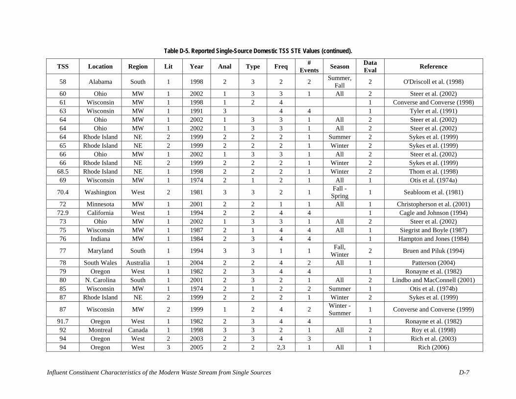
Table D-5. Reported Single-Source Domestic TSS STE Values (continued).
TSS Location Region Lit Year Anal Type Freq # Events Season Data
Eval Reference
58 Alabama South 1 1998 2 3 2 2 Summer, Fall 2 O'Driscoll et al. (1998)
60 Ohio MW 1 2002 1 3 3 1 All 2 Steer et al. (2002) 61 Wisconsin MW 1 1998 1 2 4 1 Converse and Converse (1998) 63 Wisconsin MW 1 1991 3 4 4 1 Tyler et al. (1991) 64 Ohio MW 1 2002 1 3 3 1 All 2 Steer et al. (2002) 64 Ohio MW 1 2002 1 3 3 1 All 2 Steer et al. (2002) 64 Rhode Island NE 2 1999 2 2 2 1 Summer 2 Sykes et al. (1999) 65 Rhode Island NE 2 1999 2 2 2 1 Winter 2 Sykes et al. (1999) 66 Ohio MW 1 2002 1 3 3 1 All 2 Steer et al. (2002) 66 Rhode Island NE 2 1999 2 2 2 1 Winter 2 Sykes et al. (1999)
68.5 Rhode Island NE 1 1998 2 2 2 1 Winter 2 Thom et al. (1998) 69 Wisconsin MW 1 1974 2 1 2 1 All 1 Otis et al. (1974a)
70.4 Washington West 2 1981 3 3 2 1 Fall - Spring 1 Seabloom et al. (1981)
72 Minnesota MW 1 2001 2 2 1 1 All 1 Christopherson et al. (2001) 72.9 California West 1 1994 2 2 4 4 1 Cagle and Johnson (1994) 73 Ohio MW 1 2002 1 3 3 1 All 2 Steer et al. (2002) 75 Wisconsin MW 1 1987 2 1 4 4 All 1 Siegrist and Boyle (1987) 76 Indiana MW 1 1984 2 3 4 4 1 Hampton and Jones (1984)
77 Maryland South 1 1994 3 3 1 1 Fall, Winter 2 Bruen and Piluk (1994)
78 South Wales Australia 1 2004 2 2 4 2 All 1 Patterson (2004) 79 Oregon West 1 1982 2 3 4 4 1 Ronayne et al. (1982) 80 N. Carolina South 1 2001 2 3 2 1 All 2 Lindbo and MacConnell (2001) 85 Wisconsin MW 1 1974 2 1 2 2 Summer 1 Otis et al. (1974b) 87 Rhode Island NE 2 1999 2 2 2 1 Winter 2 Sykes et al. (1999)
87 Wisconsin MW 2 1999 1 2 4 2 Winter - Summer 1 Converse and Converse (1999)
91.7 Oregon West 1 1982 2 3 4 4 1 Ronayne et al. (1982) 92 Montreal Canada 1 1998 3 3 2 1 All 2 Roy et al. (1998) 94 Oregon West 2 2003 2 3 4 3 1 Rich et al. (2003) 94 Oregon West 3 2005 2 2 2,3 1 All 1 Rich (2006)
Influent Constituent Characteristics of the Modern Waste Stream from Single Sources D-7

Table D-5. Reported Single-Source Domestic TSS STE Values (continued).
TSS Location Region Lit Year Anal Type Freq # Events Season Data
Eval Reference
102 Colorado West 3 2000 2 2 3 3 Spring 1 Siegrist et al. (2000) 72 Minnesota MW 1 2001 2 2 1 1 All 1 Christopherson et al. (2001)
133.9 Saskatch. Canada 1 1991 2 2 4 4 1 Viraraghavan and Rana (1991) 135 Wisconsin MW 1 1974 2 1 2 2 Summer 1 Otis et al. (1974b)
143 North Carolina South 1 2001 2 3 2 1 All 2 Lindbo and MacConnell (2001)
153.6 North Carolina South 1 1998 2 3 2 1 All 2 Thom et al. (1998)
161 Florida South 1 1991 2 2 1 1 Fall - Spring 1 Sherman and Anderson (1991)
163 Ohio MW 1 2002 1 3 3 1 All 2 Steer et al. (2002) 165 1 1976 3 3 4 4 2 Thiruvenkatachari (1976) 170 Perth Australia 1 1984 3 3 4 4 1 Troyan et al. (1984) 171 Oregon West 1 1982 2 3 4 4 1 Ronayne et al. (1982) 193 Oregon West 1 1982 2 3 4 4 1 Ronayne et al. (1982)
200 Alabama South 1 1998 2 3 2 2 Summer, Fall 2 O'Driscoll et al. (1998)
203 Oregon West 1 1982 2 3 4 4 1 Ronayne et al. (1982) 239 Maine NE 1 1981 2 3 4 4 1 Rock et al. (1981) 240 Oregon West 1 1982 2 3 4 4 1 Ronayne et al. (1982) 251 Colorado West 3 2000 2 2 3 3 Spring 1 Siegrist et al. (2000) 260 3 1977 3 3 4 4 2 Siegrist (1977) 276 Oregon West 1 1982 2 3 4 4 1 Ronayne et al. (1982)
blank = information not provided
D-8

Table D-6. Reported Multiple-Source Domestic TSS STE Values.
TSS Location Region Lit Year Anal Type Freq # Events Season Data
Eval Reference
27 Minnesota MW 1 2001 2 3 2 1 All 1 Henneck et al. (2001) 37 Norway Norway 1 1991 2 3 1 2 1 Siegrist et al. (1991)
46.9 Maine NE 2 1992 3 3 4 4 2 Boyer and Rock (1992) 56.7 Maine NE 2 1991 3 3 4 4 2 Boyer (1991) 60 W. Virginia South 1 1991 2 3 1 4 2 Sack et al. (1991)
60.8 Maine NE 2 1992 3 3 4 4 2 Boyer and Rock (1992) 61 Maine NE 2 1992 3 3 4 4 2 Boyer and Rock (1992)
61.2 Maine NE 2 1992 3 3 4 4 2 Boyer and Rock (1992) 63.7 Maine NE 2 1991 3 3 4 4 2 Boyer (1991) 64 Minnesota MW 1 2001 2 3 2 1 All 1 Henneck et al. (2001)
72.6 1985 3 3 4 4 2 Swed (1985) 80 New Mexico West 1 1991 3 2 4 4 1 Jacquez et al. (1991)
84.8 Ontario Canada 1 1974 3 3 1 1 All 2 Brandes et al. (1974) 93 Maine NE 2 1992 3 3 4 4 2 Boyer and Rock (1992)
95.2 Maine NE 2 1992 3 3 4 4 2 Boyer and Rock (1992) 99 Wisconsin MW 2 1991 3 2 4 4 1 Converse et al. (1991)
blank = information not provided
Table D-7. Reported Food Source TSS STE Values.
TSS Location Region Lit Year Anal Type Freq # Events Season Data
Eval Reference
12 Florida South 3 1995 1 2 4 3 2 Bloomquist and Schmidt (1995) 26 Florida South 3 1995 1 2 4 3 2 Bloomquist and Schmidt (1995) 39 Florida South 3 1995 1 2 4 3 2 Bloomquist and Schmidt (1995) 40 Florida South 3 1995 1 2 4 3 2 Bloomquist and Schmidt (1995) 42 Florida South 3 1995 1 2 4 3 2 Bloomquist and Schmidt (1995)
44.7 Florida South 3 1995 1 2 4 3 2 Bloomquist and Schmidt (1995) 46 Florida South 3 1995 1 2 4 3 2 Bloomquist and Schmidt (1995) 52 Florida South 3 1995 1 2 4 3 2 Bloomquist and Schmidt (1995) 58 Florida South 3 1995 1 2 4 3 2 Bloomquist and Schmidt (1995) 58 Florida South 3 1995 1 2 4 3 2 Bloomquist and Schmidt (1995) 60 Florida South 3 1995 1 2 4 3 2 Bloomquist and Schmidt (1995)
Influent Constituent Characteristics of the Modern Waste Stream from Single Sources D-9

Table D-7. Reported Food Source TSS STE Values (continued).
TSS Location Region Lit Year Anal Type Freq # Events Season Data
Eval Reference
60 Florida South 3 1995 1 2 4 3 2 Bloomquist and Schmidt (1995) 66.7 Florida South 3 1995 1 2 4 3 2 Bloomquist and Schmidt (1995) 72 Florida South 3 1995 1 2 4 3 2 Bloomquist and Schmidt (1995)
74.2 Mass. NE 2 1999 2 2 3 2 All 1 Higgins and Groves (1999) 87 Florida South 3 1995 1 2 4 3 2 Bloomquist and Schmidt (1995)
105 Florida South 3 1995 1 2 4 3 2 Bloomquist and Schmidt (1995) 105 Florida South 3 1995 1 2 4 3 2 Bloomquist and Schmidt (1995) 115 Florida South 3 1995 1 2 4 3 2 Bloomquist and Schmidt (1995) 127 Florida South 3 1995 1 2 4 3 2 Bloomquist and Schmidt (1995) 150 Florida South 3 1995 1 2 4 3 2 Bloomquist and Schmidt (1995) 179 Wisconsin MW 1 1984 2 2 4 4 2 Siegrist et al. (1984b) 187 Florida South 3 1995 1 2 4 3 2 Bloomquist and Schmidt (1995) 190 Florida South 3 1995 1 2 4 3 2 Bloomquist and Schmidt (1995) 210 Florida South 3 1995 1 2 4 3 2 Bloomquist and Schmidt (1995) 220 Florida South 3 1995 1 2 4 3 2 Bloomquist and Schmidt (1995) 237 Florida South 3 1995 1 2 4 3 2 Bloomquist and Schmidt (1995) 245 Wisconsin MW 1 1984 2 2 4 4 2 Siegrist et al. (1984b) 247 Florida South 3 1995 1 2 4 3 2 Bloomquist and Schmidt (1995) 261 Wisconsin MW 1 1984 2 2 4 4 2 Siegrist et al. (1984b) 264 Florida South 3 1995 1 2 4 3 2 Bloomquist and Schmidt (1995) 328 Florida South 3 1995 1 2 4 3 2 Bloomquist and Schmidt (1995) 377 Wisconsin MW 1 1984 2 2 4 4 2 Siegrist et al. (1984b) 410 Mass. NE 2 1999 2 2 3 2 All 1 Higgins and Groves (1999) 413 Florida South 3 1995 1 2 4 3 2 Bloomquist and Schmidt (1995) 458 Florida South 3 1995 1 2 4 3 2 Bloomquist and Schmidt (1995) 465 Florida South 3 1995 1 2 4 3 2 Bloomquist and Schmidt (1995)
493 Maine, Ontario
NE, Canada 1 1994 3 2 2 1 All 1 McKee and Brooks (1994)
515 Florida South 3 1995 1 2 4 3 2 Bloomquist and Schmidt (1995) 582 Wisconsin MW 1 1984 2 2 4 4 2 Siegrist et al. (1984b) 644 Florida South 3 1995 1 2 4 3 2 Bloomquist and Schmidt (1995)
D-100

Table D-7. Reported Food Source TSS STE Values (continued).
TSS Location Region Lit Year Anal Type Freq # Events Season Data
Eval Reference
693 Wisconsin MW 1 1984 2 2 4 4 2 Siegrist et al. (1984b) 792.5 Massachusetts NE 2 1999 2 2 3 2 All 1 Higgins and Groves (1999) 880 Wisconsin MW 1 1984 2 2 4 4 2 Siegrist et al. (1984b) 4775 Florida South 3 1995 1 2 4 3 2 Bloomquist and Schmidt (1995)
blank = information not provided
Table D-8. Reported Non-medical Source TSS STE Values.
TSS Location Region Lit Year Anal Type Freq # Events Season Data
Eval Source Type Reference
13.8 Mass. NE 2 1999 2 2 3 2 All 1 School Higgins and Groves (1999)
15.5 Mass. NE 2 1999 2 2 3 2 All 1 School Higgins and Groves (1999)
21 Mass. NE 2 1999 2 2 3 2 All 1 School Higgins and Groves (1999)
28 Oregon, Arizona West 2 1999 3 3 4 4 2 Convenience
Store Ball et al. (1999)
30 New Mexico West 2 2002 3 3 4 4 2 School Egemen et al. (2002)
31.8 Mass. NE 2 1999 2 2 3 2 All 1 School Higgins and Groves (1999)
33 Oregon West 1 1982 2 3 4 4 1 Office Ronayne et al. (1982)
33.5 Mass. NE 2 1999 2 2 3 2 All 1 School Higgins and Groves (1999)
34 Minnesota MW 2 1999 2 3 2 1 Winter - Summer 1 Correctional
Facility McCarthy et al.
(1999)
34 Minnesota MW 2 1999 2 3 2 1 Winter - Summer 1 Correctional
Facility McCarthy et al.
(1999)
36 Minnesota MW 2 1999 2 3 2 1 Winter - Summer 1 Correctional
Facility McCarthy et al.
(1999)
36 Minnesota MW 2 1999 2 3 2 1 Winter - Summer 1 Correctional
Facility McCarthy et al.
(1999)
Influent Constituent Characteristics of the Modern Waste Stream from Single Sources D-111

Table D-8. Reported Non-medical Source TSS STE Values (continued).
TSS Location Region Lit Year Anal Type Freq # Events Season Data
Eval Source Type Reference
37 Minnesota MW 2 1999 2 3 2 1 Winter - Summer 1 Correctional
Facility McCarthy et al.
(1999)
37 Minnesota MW 2 1999 2 3 2 1 Winter - Summer 1 Correctional
Facility McCarthy et al.
(1999)
38 Minnesota MW 2 1999 2 3 2 1 Winter - Summer 1 Correctional
Facility McCarthy et al.
(1999)
38.4 Mass. NE 2 1999 2 2 3 2 All 1 School Higgins and Groves (1999)
39 Minnesota MW 2 1999 2 3 2 1 Winter - Summer 1 Correctional
Facility McCarthy et al.
(1999)
39 Minnesota MW 2 1999 2 3 2 1 Winter - Summer 1 Correctional
Facility McCarthy et al.
(1999)
39 Minnesota MW 2 1999 2 3 2 1 Winter - Summer 1 Correctional
Facility McCarthy et al.
(1999)
39.6 Oregon West 1 1982 2 3 4 4 1 Sawmill Ronayne et al. (1982)
41.8 Pennsylvania NE 1 2003 2 2 4 4 1 Camp Whitehill et al. (2003)
44 Wisconsin MW 1 1984 2 2 4 4 2 Golf club Siegrist et al. (1984b)
44.7 Mass. NE 2 1999 2 2 3 2 All 1 Office Higgins and Groves (1999)
46 Minnesota MW 1 2001 2 3 2 1 All 1 Correctional Facility
Henneck et al. (2001)
50 Wisconsin MW 1 1994 2 1 2 1 All 1 Correctional institution Boyle et al. (1994)
52 Minnesota MW 2 1999 2 3 2 1 Winter - Summer 1 Correctional
Facility McCarthy et al.
(1999)
52 Minnesota MW 2 1999 2 3 2 1 Winter - Summer 1 Correctional
Facility McCarthy et al.
(1999)
53 Minnesota MW 2 1999 2 3 2 1 Winter - Summer 1 Correctional
Facility McCarthy et al.
(1999)
53 Minnesota MW 2 1999 2 3 2 1 Winter - Summer 1 Correctional
Facility McCarthy et al.
(1999)
54 Minnesota MW 2 1999 2 3 2 1 Winter - Summer 1 Correctional
Facility McCarthy et al.
(1999)
D-122

Table D-8. Reported Non-medical Source TSS STE Values (continued).
TSS Location Region Lit Year Anal Type Freq # Events Season Data
Eval Source Type Reference
54 Minnesota MW 2 1999 2 3 2 1 Winter - Summer 1 Correctional
Facility McCarthy et al.
(1999)
55 Oregon, Arizona West 2 1999 3 3 4 4 2 Camp Ball et al. (1999)
55.6 Mass. NE 2 1999 2 2 3 2 All 1 Office Higgins and Groves (1999)
56 Wisconsin MW 1 1984 2 2 4 4 2 Golf club Siegrist et al. (1984b)
66 Wisconsin MW 1 1984 2 2 4 4 2 Motel Siegrist et al. (1984b)
75 Minnesota MW 2 1999 2 3 2 1 Winter - Summer 1 Correctional
Facility McCarthy et al.
(1999)
83.6 Mass. NE 2 1999 2 2 3 2 All 1 Office Higgins and Groves (1999)
107.6 Mass. NE 2 1999 2 2 3 2 All 1 School Higgins and Groves (1999)
118.7 Pennsylvania NE 1 2003 2 2 4 4 1 Grocery store with meat packing
Whitehill et al. (2003)
121 Wisconsin MW 1 1984 2 2 4 4 2 Golf club Siegrist et al. (1984b)
150.3 Virginia South 2 2002 3 3 4 4 2
One room schoolhouse turned into museum
Hatch et al. (2002)
blank = information not provided
Influent Constituent Characteristics of the Modern Waste Stream from Single Sources D-133
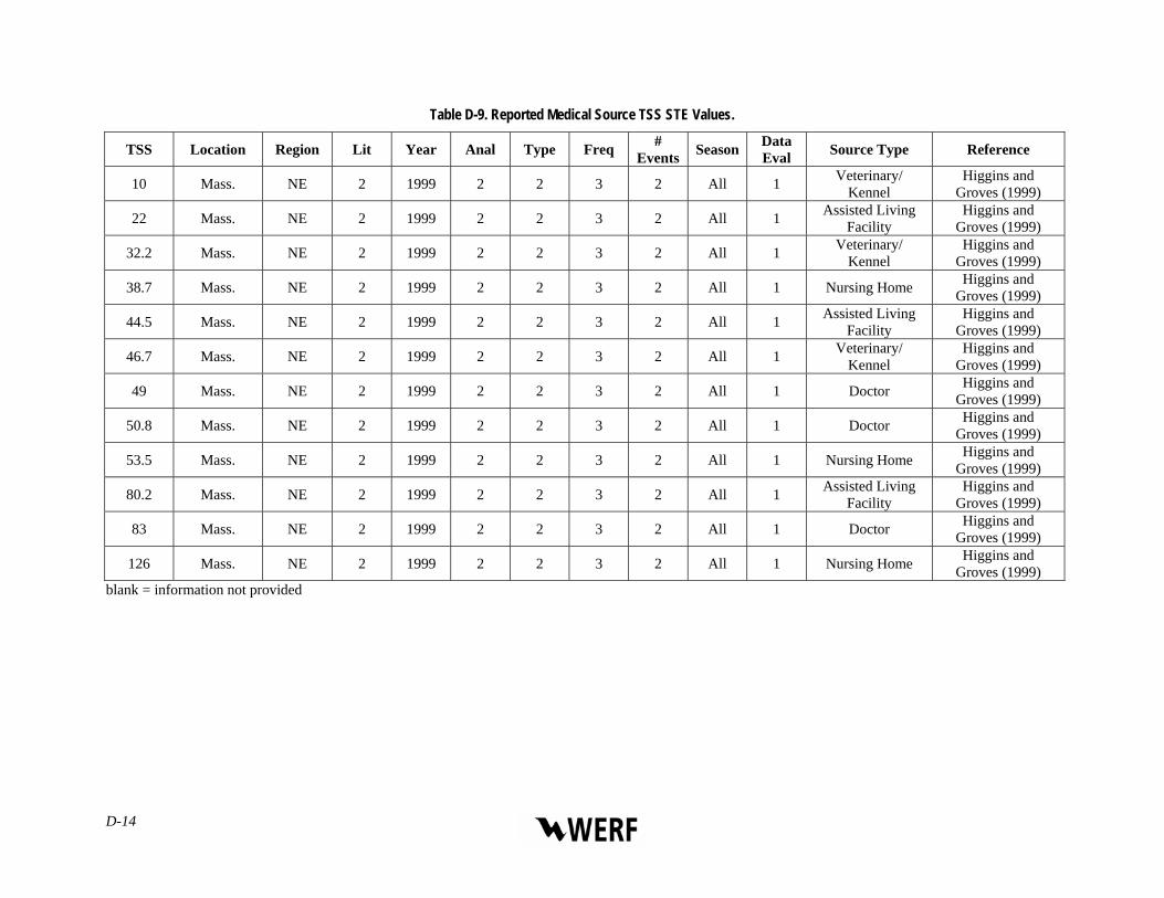
Table D-9. Reported Medical Source TSS STE Values.
TSS Location Region Lit Year Anal Type Freq # Events Season Data
Eval Source Type Reference
10 Mass. NE 2 1999 2 2 3 2 All 1 Veterinary/ Kennel
Higgins and Groves (1999)
22 Mass. NE 2 1999 2 2 3 2 All 1 Assisted Living Facility
Higgins and Groves (1999)
32.2 Mass. NE 2 1999 2 2 3 2 All 1 Veterinary/ Kennel
Higgins and Groves (1999)
38.7 Mass. NE 2 1999 2 2 3 2 All 1 Nursing Home Higgins and Groves (1999)
44.5 Mass. NE 2 1999 2 2 3 2 All 1 Assisted Living Facility
Higgins and Groves (1999)
46.7 Mass. NE 2 1999 2 2 3 2 All 1 Veterinary/ Kennel
Higgins and Groves (1999)
49 Mass. NE 2 1999 2 2 3 2 All 1 Doctor Higgins and Groves (1999)
50.8 Mass. NE 2 1999 2 2 3 2 All 1 Doctor Higgins and Groves (1999)
53.5 Mass. NE 2 1999 2 2 3 2 All 1 Nursing Home Higgins and Groves (1999)
80.2 Mass. NE 2 1999 2 2 3 2 All 1 Assisted Living Facility
Higgins and Groves (1999)
83 Mass. NE 2 1999 2 2 3 2 All 1 Doctor Higgins and Groves (1999)
126 Mass. NE 2 1999 2 2 3 2 All 1 Nursing Home Higgins and Groves (1999)
blank = information not provided
D-144

Table D-8. Reported Non-medical Source TSS STE Values (continued).
TSS Location Region Lit Year Anal Type Freq # Events Season Data
Eval Source Type Reference
54 Minnesota MW 2 1999 2 3 2 1 Winter - Summer 1 Correctional
Facility McCarthy et al.
(1999)
55 Oregon, Arizona West 2 1999 3 3 4 4 2 Camp Ball et al. (1999)
55.6 Mass. NE 2 1999 2 2 3 2 All 1 Office Higgins and Groves (1999)
56 Wisconsin MW 1 1984 2 2 4 4 2 Golf club Siegrist et al. (1984b)
66 Wisconsin MW 1 1984 2 2 4 4 2 Motel Siegrist et al. (1984b)
75 Minnesota MW 2 1999 2 3 2 1 Winter - Summer 1 Correctional
Facility McCarthy et al.
(1999)
83.6 Mass. NE 2 1999 2 2 3 2 All 1 Office Higgins and Groves (1999)
107.6 Mass. NE 2 1999 2 2 3 2 All 1 School Higgins and Groves (1999)
118.7 Pennsylvania NE 1 2003 2 2 4 4 1 Grocery store with meat packing
Whitehill et al. (2003)
121 Wisconsin MW 1 1984 2 2 4 4 2 Golf club Siegrist et al. (1984b)
150.3 Virginia South 2 2002 3 3 4 4 2
One room schoolhouse turned into museum
Hatch et al. (2002)
blank = information not provided
Influent Constituent Characteristics of the Modern Waste Stream from Single Sources D-153

Table D-10. Reported Municipal Source TSS Raw Wastewater and STE Values (continued).
TSS (mg/L) Sample Description Reference 316 Influent Sadler et al. (2002)
338.3 After Screen Curto et al. (2002) 359 Influent Littleton et al. (2003) 385 Influent Danielson (2006) 428 Raw Wastewater Crawford et al. (2000) 444 Influent Zheng et al. (2002) 635 Influent Zheng et al. (2002)
1700 Wastewater Characteristics Gale (2002) 2003 Raw Wastewater Xingcan et al. (2001)
Table D-11. Other Reported Solids Values.
Average Value Constituent (units) Source Waste Stream Reference 788 Total Solids (mg/L) Raw Single-source domestic Watson et al. (1967) 859 Total Solids (mg/L) Raw Single-source domestic Watson et al. (1967) 866 Total Solids (mg/L) Raw Single-source domestic Watson et al. (1967) 997 Total Solids (mg/L) Raw Single-source domestic Watson et al. (1967) 1180 Total Solids (mg/L) Raw Single-source domestic Bennett et al. (1974) 1249 Total Solids (mg/L) Raw Single-source domestic Watson et al. (1967) 1536 Total Solids (mg/L) Raw Single-source domestic Watson et al. (1967) 1710 Total Solids (mg/L) Raw Non-medical, Rest Area Restroom Pearson et al. (1987) 6460 Total Solids (mg/L) Raw Non-medical, RV Dump Pearson et al. (1987) 339 Total Solids (mg/L) STE Single-source domestic Seabloom et al. (1981) 366 Total Solids (mg/L) STE Single-source domestic Seabloom et al. (1981) 428 Total Solids (mg/L) STE Single-source domestic Seabloom et al. (1981) 452 Total Solids (mg/L) STE Single-source domestic Seabloom et al. (1981) 502 Total Solids (mg/L) STE Single-source domestic Tyler et al. (1991) 728 Total Solids (mg/L) STE Single-source domestic Tyler et al. (1991) 913 Total Solids (mg/L) STE Single-source domestic Karikari et al. (1974) 969 Total Solids (mg/L) STE Single-source domestic Hampton and Jones (1984) 1090 Total Solids (mg/L) STE Single-source domestic Converse and Converse (1998) 1268 Total Solids (mg/L) STE Single-source domestic Converse et al. (1994) 1594 Total Solids (mg/L) STE Single-source domestic Hampton and Jones (1984)
D-16

Table D-11. Other Reported Solids Values (continued).
Average Value Constituent (units) Source Waste Stream Reference 1608 Total Solids (mg/L) STE Single-source domestic Siegrist and Boyle (1987) 413 Total Solids (mg/L) STE Multiple-source domestic Siegrist et al. (1991) 1271 Total Solids (mg/L) STE Multiple-source domestic Converse et al. (1991) 653 Total Dissolved Solids (mg/L) Raw Single-source domestic Edvardsson and Spears (2000) 836 Total Dissolved Solids (mg/L) Raw Multiple-source domestic Anderson and Siegrist (1989) 1074 Total Dissolved Solids (mg/L) Raw Multiple-source domestic Anderson and Siegrist (1989) 575 Total Dissolved Solids (mg/L) STE Single-source domestic Duncan et al. (1994) 615 Total Dissolved Solids (mg/L) STE Single-source domestic Reneau et al. (2001) 674 Total Dissolved Solids (mg/L) STE Single-source domestic Huang et al. (1994) 344 Total Dissolved Solids (mg/L) STE Non-medical, Correctional Institute Boyle et al. (1994)
497 Total Dissolved Solids (mg/L) STE Non-medical, Campus Christian Center & Dorm Anderson et al. (1994)
414 Total Volatile Solids (mg/L) Raw Single-source domestic Watson et al. (1967) 468 Total Volatile Solids (mg/L) Raw Single-source domestic Watson et al. (1967) 485 Total Volatile Solids (mg/L) Raw Single-source domestic Watson et al. (1967) 571 Total Volatile Solids (mg/L) Raw Single-source domestic Watson et al. (1967) 659 Total Volatile Solids (mg/L) Raw Single-source domestic Watson et al. (1967) 942 Total Volatile Solids (mg/L) Raw Single-source domestic Watson et al. (1967) 357 Total Volatile Solids (mg/L) STE Single-source domestic Hampton and Jones (1984) 381 Total Volatile Solids (mg/L) STE Single-source domestic Hampton and Jones (1984) 1114 Volatile Solids (mg/L) Raw Non-medical, Rest Area Restroom Pearson et al. (1987) 4353 Volatile Solids (mg/L) Raw Non-medical, RV Dump Pearson et al. (1987) 261 Volatile Solids (mg/L) STE Single-source domestic Converse and Converse (1998) 263 Volatile Solids (mg/L) STE Single-source domestic Tyler et al. (1991) 271 Volatile Solids (mg/L) STE Single-source domestic Tyler et al. (1991) 273 Volatile Solids (mg/L) STE Single-source domestic Converse et al. (1994) 295 Volatile Solids (mg/L) STE Single-source domestic Siegrist and Boyle (1987) 402 Volatile Solids (mg/L) STE Multiple-source domestic Converse et al. (1991) 203 Volatile Suspended Solids (mg/L) Raw Single-source domestic Ziebell et al. (1974) 642 Volatile Suspended Solids (mg/L) Raw Non-medical, Rest Area Restroom Pearson et al. (1987) 2460 Volatile Suspended Solids (mg/L) Raw Non-medical, RV Dump Pearson et al. (1987) 3329 Volatile Suspended Solids (mg/L) Raw Non-medical, RV Dump Pearson et al. (1987) 15.1 Volatile Suspended Solids (mg/L) STE Single-source domestic Seabloom et al. (1981)
Influent Constituent Characteristics of the Modern Waste Stream from Single Sources D-17

D-18
Table D-11. Other Reported Solids Values (continued).
Average Value Constituent (units) Source Waste Stream Reference 16.9 Volatile Suspended Solids (mg/L) STE Single-source domestic Seabloom et al. (1981) 19.3 Volatile Suspended Solids (mg/L) STE Single-source domestic Seabloom et al. (1981) 25 Volatile Suspended Solids (mg/L) STE Single-source domestic Tyler et al. (1991)
27.7 Volatile Suspended Solids (mg/L) STE Single-source domestic Thom et al. (1998) 29 Volatile Suspended Solids (mg/L) STE Single-source domestic Converse et al. (1994) 33 Volatile Suspended Solids (mg/L) STE Single-source domestic Sauer et al. (1976)
35.5 Volatile Suspended Solids (mg/L) STE Single-source domestic Ziebell et al. (1974) 37 Volatile Suspended Solids (mg/L) STE Single- source domestic Hargett et al. (1981) 40 Volatile Suspended Solids (mg/L) STE Single-source domestic Hampton and Jones (1984) 46 Volatile Suspended Solids (mg/L) STE Single-source domestic Converse and Converse (1998) 46 Volatile Suspended Solids (mg/L) STE Single-source domestic Hampton and Jones (1984) 49 Volatile Suspended Solids (mg/L) STE Single-source domestic Tyler et al. (1991)
54.6 Volatile Suspended Solids (mg/L) STE Single-source domestic Seabloom et al. (1981) 56.8 Volatile Suspended Solids (mg/L) STE Single-source domestic Thom et al. (1998) 60 Volatile Suspended Solids (mg/L) STE Single-source domestic Converse and Converse (1999) 62 Volatile Suspended Solids (mg/L) STE Single-source domestic Siegrist and Boyle (1987)
65.3 Volatile Suspended Solids (mg/L) STE Single-source domestic Thom et al. (1998) 23.8 Volatile Suspended Solids (mg/L) STE Multiple-source domestic Neralla et al. (1998) 60 Volatile Suspended Solids (mg/L) STE Multiple-source domestic Converse et al. (1991) 33 Volatile Suspended Solids (mg/L) STE Non-medical, Lab (simulated household) Siegrist (1978) 46 Volatile Suspended Solids (mg/L) STE Non-medical, Correctional Institute Boyle et al. (1994)
149 Volatile Dissolved Solids (mg/L) STE Non-medical, Correctional Institute Boyle et al. (1994)
APPENDIX E
COMPLETE LISTING OF REPORTED NUTRIENT (NITROGEN AND PHOSPHORUS) VALUES
Influent Constituent Characteristics of the Modern Waste Stream from Single Sources E-1

E-2
Tables E-1 through E-19 summarize the reported values and the data qualifiers used. The following key should be used to interpret the data qualifier information within the tables. A more detailed description of the data qualifiers can be found in the report, Section 3.4.1.
Location = state where the study was conducted
Region = location of the study based on US Census defined regions MW = Midwest: IL, IN, IA, KS, MI, MN, MO, NE, ND, OH, SD, and WI NE = Northeast: CT, ME, MA, NH, NJ, NY, PA, RI, VT South: AL, AR, DE, DC, FL, GA, KY, LA, MD, MS, NC, OK, SC, TN, TX, VA, and WV West: AK, AZ, CA, CO, HI, ID, MT, NV, NM, OR, UT, WA, and WY
Lit = literature source 1 – publicly available and published in a peer reviewed journal 2 – publicly available and published in conference proceedings or project report 3 – unpublished; information obtained directly from researcher and is not publicly available
Year = year the study was conducted
Anal = analytical method used 1 – detailed methods used = specified which approved method was used (e.g., APHA 4500-N B). 2 – standard methods = specified use of approved methods (e.g., APHA). 3 – no methods = did not specify which method was used
Type = sampling technique used 1 – composite sample collected 2 – grab sample collected 3 – unknown; type of sample collected was not specified
Freq = frequency of sample collection 1 – at least weekly 2 – bi-weekly to monthly 3 – less than one time per month 4 – unknown
# Events = number of sampling events 1 – more than 12 sampling events reported 2 – between 3 and 12 sampling events reported 3 – less than 3 sampling events reported 4 – unknown; number of sampling events not reported
Season = time of year when study was conducted Spring (Mar-May) Summer (Jun-Aug) Fall (Sept-Nov) Winter (Dec-Feb) All (Jan-Dec)
Data Eval = data evaluation 1 –more than a single average value reported (e.g., descriptive statistics provided) 2 – only the average value reported for each constituent
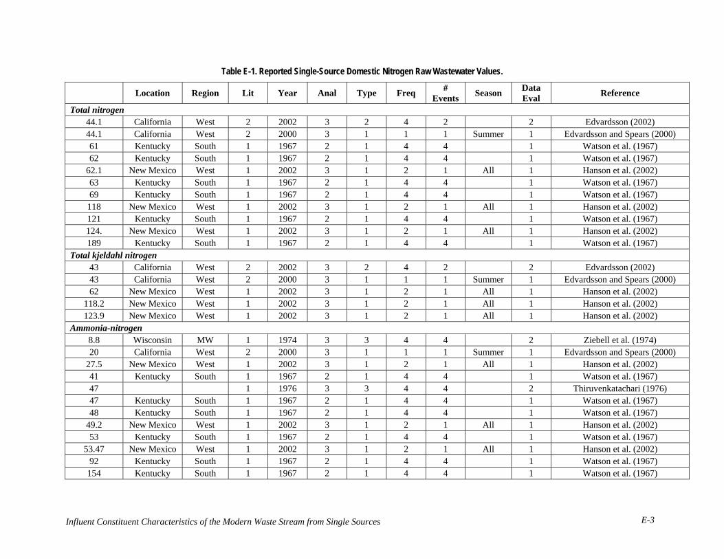
Table E-1. Reported Single-Source Domestic Nitrogen Raw Wastewater Values.
Location Region Lit Year Anal Type Freq # Events Season Data
Eval Reference
Total nitrogen 44.1 California West 2 2002 3 2 4 2 2 Edvardsson (2002) 44.1 California West 2 2000 3 1 1 1 Summer 1 Edvardsson and Spears (2000) 61 Kentucky South 1 1967 2 1 4 4 1 Watson et al. (1967) 62 Kentucky South 1 1967 2 1 4 4 1 Watson et al. (1967)
62.1 New Mexico West 1 2002 3 1 2 1 All 1 Hanson et al. (2002) 63 Kentucky South 1 1967 2 1 4 4 1 Watson et al. (1967) 69 Kentucky South 1 1967 2 1 4 4 1 Watson et al. (1967) 118 New Mexico West 1 2002 3 1 2 1 All 1 Hanson et al. (2002) 121 Kentucky South 1 1967 2 1 4 4 1 Watson et al. (1967) 124. New Mexico West 1 2002 3 1 2 1 All 1 Hanson et al. (2002) 189 Kentucky South 1 1967 2 1 4 4 1 Watson et al. (1967)
Total kjeldahl nitrogen 43 California West 2 2002 3 2 4 2 2 Edvardsson (2002) 43 California West 2 2000 3 1 1 1 Summer 1 Edvardsson and Spears (2000) 62 New Mexico West 1 2002 3 1 2 1 All 1 Hanson et al. (2002)
118.2 New Mexico West 1 2002 3 1 2 1 All 1 Hanson et al. (2002) 123.9 New Mexico West 1 2002 3 1 2 1 All 1 Hanson et al. (2002)
Ammonia-nitrogen 8.8 Wisconsin MW 1 1974 3 3 4 4 2 Ziebell et al. (1974) 20 California West 2 2000 3 1 1 1 Summer 1 Edvardsson and Spears (2000)
27.5 New Mexico West 1 2002 3 1 2 1 All 1 Hanson et al. (2002) 41 Kentucky South 1 1967 2 1 4 4 1 Watson et al. (1967) 47 1 1976 3 3 4 4 2 Thiruvenkatachari (1976) 47 Kentucky South 1 1967 2 1 4 4 1 Watson et al. (1967) 48 Kentucky South 1 1967 2 1 4 4 1 Watson et al. (1967)
49.2 New Mexico West 1 2002 3 1 2 1 All 1 Hanson et al. (2002) 53 Kentucky South 1 1967 2 1 4 4 1 Watson et al. (1967)
53.47 New Mexico West 1 2002 3 1 2 1 All 1 Hanson et al. (2002) 92 Kentucky South 1 1967 2 1 4 4 1 Watson et al. (1967) 154 Kentucky South 1 1967 2 1 4 4 1 Watson et al. (1967)
Influent Constituent Characteristics of the Modern Waste Stream from Single Sources E-3

Table E-1. Reported Single-Source Domestic Nitrogen Raw Wastewater Values (continued).
Location Region Lit Year Anal Type Freq # Events Season Data
Eval Reference
Nitrate-nitrogen 0.05 New Mexico West 1 2002 3 1 2 1 All 1 Hanson et al. (2002) 0.05 New Mexico West 1 2002 3 1 2 1 All 1 Hanson et al. (2002)
0.1575 New Mexico West 1 2002 3 1 2 1 All 1 Hanson et al. (2002) 1.1 California West 2 2002 3 2 4 2 2 Edvardsson (2002) 1.1 California West 2 2000 3 1 1 1 Summer 1 Edvardsson and Spears (2000)
blank = information not provided
Table E-2. Reported Multiple-Source Domestic Nitrogen Raw Wastewater Values.
Location Region Lit Year Anal Type Freq # Events Season Data
Eval Reference
Total nitrogen
39 Michigan/British Columbia
MW, Canada 2 2002 1 1 4 4 1 Bell and Higgins (2004)
80 Wisconsin MW 2 1978 2 3 4 4 1 Siegrist (1978) Total kjeldahl nitrogen
53 Arizona West 1 1989 2 1 1 2 Fall 1 Anderson and Siegrist (1989) 55 Arizona West 1 1989 2 1 1 2 Fall 1 Anderson and Siegrist (1989)
blank = information not provided
E-4

Table E-3. Reported Multiple-Source Domestic Nitrogen Raw Wastewater Values.
Location Region Lit Year Anal Type Freq # Events Season Data
Eval Source Type Reference
Total nitrogen
38.61 Florida South 1 1998 2 1 2 2 Winter - Summer 1 Min. Security
Correctional Inst. Anderson et al.
(1998) Total kjeldahl nitrogen
38.58 Florida South 1 1998 2 1 2 2 Winter - Summer 1 Min. Security
Correctional Inst. Anderson et al.
(1998)
116 Louisiana South 2 2002 1 3 2 1 All 1 RV Dump/ Rest Area Griffin et al. (2002)
119 Louisiana South 2 2004 3 3 4 4 1 RV Dump/ Rest Area Griffin et al. (2004)
Ammonia-nitrogen
32.2 Louisiana South 2 2002 1 3 2 1 All 1 RV Dump/ Rest Area Griffin et al. (2002)
40.35 Louisiana South 2 2004 3 3 4 4 1 RV Dump/ Rest Area Griffin et al. (2004)
315 California West 2 1987 3 3 4 4 2 Rest Area Pearson et al. (1987)
767 California West 2 1987 3 3 4 4 2 RV Dump Pearson et al. (1987)
blank = information not provided
Table E-4. Reported Single-Source Domestic Nitrogen STE Values.
Location Region Lit Year Anal Type Freq # Events Season Data
Eval Reference
Total nitrogen
26 Alabama South 1 1998 2 3 2 2 Summer, Fall 2 O'Driscoll et al. (1998)
34 Alabama South 1 1998 2 3 2 2 Summer, Fall 2 O'Driscoll et al. (1998)
39 Rhode Island NE 2 1999 2 2 2 1 Summer 2 Sykes et al. (1999) 40.2 Wisconsin MW 1 1974 2 1 2 1 All 1 Otis et al. (1974a) 41.5 Ohio MW 1 1984 2 1 1 1 All 1 Effert et al. (1984)
41.7 Maryland South 1 1994 3 3 1 1 Fall, Winter 2 Bruen and Piluk (1994)
Influent Constituent Characteristics of the Modern Waste Stream from Single Sources E-5

Table E-4. Reported Single-Source Domestic Nitrogen STE Values (continued).
Location Region Lit Year Anal Type Freq # Events Season Data
Eval Reference
Total nitrogen (continued) 43 Rhode Island NE 2 1999 2 2 2 1 Summer 2 Sykes et al. (1999) 45 Rhode Island NE 2 1999 2 2 2 1 Summer 2 Sykes et al. (1999)
45.67 Oregon West 1 1982 2 3 4 4 1 Ronayne et al. (1982) 46.2 Kentucky South 1 1998 2 3 2 1 All 1 Thom et al. (1998) 47 Minnesota MW 1 2001 2 2 1 1 All 1 Christopherson et al. (2001)
47.2 Oregon West 1 1982 2 3 4 4 1 Ronayne et al. (1982) 48.7 Maine, Ontario NE, Canada 1 1994 3 2 2 1 All 1 McKee and Brooks (1994) 49.9 Maine, Ontario NE, Canada 1 1998 3 2 2 1 All 1 Thom et al. (1998) 50 Rhode Island NE 2 1999 2 2 2 1 Winter 2 Sykes et al. (1999)
50.5 Wisconsin MW 1 1974 2 1 2 1 All 1 Otis et al. (1974a) 51 Minnesota MW 1 2001 2 2 1 1 All 1 Christopherson et al. (2001)
51.8 Oregon West 1 1982 2 3 4 4 1 Ronayne et al. (1982) 52.2 Wisconsin MW 2 1999 3 3 4 4 2 Converse (1999) 53 Rhode Island NE 2 1999 2 2 2 1 Winter 2 Sykes et al. (1999)
53.1 Washington West 1 2000 2 3 4 4 2 Harrison et al. (2000) 54 Rhode Island NE 2 1999 2 2 2 1 Winter 2 Sykes et al. (1999)
56.7 Wisconsin MW 1 1974 2 1 2 1 All 1 Otis et al. (1974a) 57.1 Oregon West 1 1982 2 3 4 4 1 Ronayne et al. (1982) 57.8 Wisconsin MW 1 1974 2 1 2 1 All 1 Otis et al. (1974a) 59.2 Oregon West 1 1982 2 3 4 4 1 Ronayne et al. (1982) 59.5 New Mexico West 1 2002 3 1 2 1 All 1 Hanson et al. (2002) 61.8 California West 1 1994 2 2 4 4 1 Cagle and Johnson (1994) 62 3 1977 3 3 4 4 2 Siegrist (1977) 62 Colorado West 3 2000 2 2 3 3 Spring 1 Siegrist et al. (2000) 63 Oregon West 2 2003 2 3 4 3 1 Rich et al. (2003) 63 Rhode Island NE 2 2002 2 3 2 3 All 1 Loomis et al. (2002)
65.2 Maine, Ontario NE, Canada 1 1994 3 2 2 1 All 1 McKee and Brooks (1994) 66 Oregon West 3 2005 2 2 2,3 1 All 1 Rich (2006) 67 Oregon West 2 2003 2 3 4 3 1 Rich et al. (2003) 67 Rhode Island NE 1 2001 2 3 2 2 All 1 Bohrer and Converse (2001)
E-6

Table E-4. Reported Single-Source Domestic Nitrogen STE Values (continued).
Location Region Lit Year Anal Type Freq # Events Season Data
Eval Reference
Total nitrogen (continued)
68.6 Maine, Ontario
NE, Canada 1 1994 3 2 2 1 All 1 McKee and Brooks (1994)
69 Colorado West 3 2000 2 2 3 3 Spring 1 Siegrist et al. (2000)
70.3 Maine, Ontario
NE, Canada 1 1998 3 2 2 1 All 1 Thom et al. (1998)
70.9 Oregon West 1 1982 2 3 4 4 1 Ronayne et al. (1982) 71.9 Oregon West 1 1982 2 3 4 4 1 Ronayne et al. (1982) 73 Iowa MW 1 1974 3 2 1 2 2 Karikari et al. (1974)
85.8 South Wales Australia 1 2004 2 2 4 2 All 1 Patterson (2004) 91.8 South Wales Australia 1 2000 2 2 4 2 1 Harrison et al. (2000) 124 South Wales Australia 1 2000 2 2 4 2 1 Harrison et al. (2000)
Total kjeldahl nitrogen 27 N. Carolina South 1 2001 2 3 2 1 All 2 Lindbo and MacConnell (2001)
28.8 N. Carolina South 1 2001 2 3 2 1 All 2 Lindbo and MacConnell (2001)
39 Florida South 1 1991 2 2 1 1 Fall - Spring 1 Sherman and Anderson (1991)
41.6 Maryland South 1 1994 3 3 1 1 Fall, Winter 2 Bruen and Piluk (1994)
42 Montreal Canada 1 1998 3 3 2 1 All 2 Roy et al. (1998)
45.6 Virginia South 1 1994 1 3 2 2 Fall - Spring 2 Huang et al. (1994)
45.6 Oregon West 1 1982 2 3 4 4 1 Ronayne et al. (1982) 46.2 Virginia South 1 2001 2 2 4 4 2 Reneau et al. (2001) 46.8 Saskatch. Canada 1 1991 2 2 4 4 1 Viraraghavan and Rana (1991) 47.2 Oregon West 1 1982 2 3 4 4 1 Ronayne et al. (1982) 47.7 Virginia South 1 2001 2 2 4 4 2 Reneau et al. (2001) 51.3 Oregon West 1 1982 2 3 4 4 1 Ronayne et al. (1982) 52 Wisconsin MW 2 1999 3 3 4 4 2 Converse (1999)
56.9 Oregon West 1 1982 2 3 4 4 1 Ronayne et al. (1982) 58 Wisconsin MW 1 1998 1 2 4 1 Converse and Converse (1998)
58.4 Oregon West 1 1982 2 3 4 4 1 Ronayne et al. (1982) 58.65 New Mexico West 1 2002 3 1 2 1 All 1 Hanson et al. (2002)
Influent Constituent Characteristics of the Modern Waste Stream from Single Sources E-7

Table E-4. Reported Single-Source Domestic Nitrogen STE Values (continued).
Location Region Lit Year Anal Type Freq # Events Season Data
Eval Reference
Total kjeldahl nitrogen (continued) 60.7 Wisconsin MW 1 1987 2 1 4 4 All 1 Siegrist and Boyle (1987) 61.8 California West 1 1994 2 2 4 4 1 Cagle and Johnson (1994)
62 Wisconsin MW 2 1999 1 2 4 2 Winter - Summer 1 Converse and Converse (1999)
66 Oregon West 1 1994 3 3 1 1 All 2 Ball (1994) 70.5 Oregon West 1 1982 2 3 4 4 1 Ronayne et al. (1982) 71.8 Oregon West 1 1982 2 3 4 4 1 Ronayne et al. (1982) 75 South Wales Australia 1 2004 2 2 4 2 All 1 Patterson (2004)
94.4 California West 1980 3 3 4 2 Winter 2 Baker (1980) Ammonia-nitrogen
0 Oregon West 1 1982 2 3 4 4 1 Ronayne et al. (1982) 5.6 Ohio MW 1 2002 1 3 3 1 All 2 Steer et al. (2002)
16.2 Washington West 2 1981 3 3 2 1 Fall - Spring 1 Seabloom et al. (1981)
18.7 N. Carolina South 1 2001 2 3 2 1 All 2 Lindbo and MacConnell (2001) 18.9 N. Carolina South 1 2000 2 3 2 1 2 Harrison et al. (2000)
19 Wisconsin MW 1 1977 3 3 4 4 Spring, Summer 1 Sauer and Boyle (1977)
20.3 Ohio MW 1 2002 1 3 3 1 All 2 Steer et al. (2002) 20.9 1 1976 3 3 4 4 2 Sauer et al. (1976)
21 Wisconsin MW 1 1977 3 3 4 4 Fall, Winter 1 Sauer and Boyle (1977)
21.3 Ohio MW 1 2002 1 3 3 1 All 2 Steer et al. (2002) 22.4 Washington West 1 2000 2 3 4 4 2 Harrison et al. (2000)
23.3 Washington West 2 1981 3 3 2 1 Fall - Spring 1 Seabloom et al. (1981)
24.3 N. Carolina South 1 2001 2 3 2 1 All 2 Lindbo and MacConnell (2001)
26 Wisconsin MW 1 1977 3 3 4 4 Summer, Fall 1 Sauer and Boyle (1977)
26.2 Washington West 2 1981 3 3 2 1 Fall - Spring 1 Seabloom et al. (1981)
26.5 Ohio MW 1 2002 1 3 3 1 All 2 Steer et al. (2002)
E-8

Table E-4. Reported Single-Source Domestic Nitrogen STE Values (continued).
Location Region Lit Year Anal Type Freq # Events Season Data
Eval Reference
Ammonia-nitrogen (continued) 26.8 Oregon West 1 1982 2 3 4 4 1 Ronayne et al. (1982) 27.8 Ohio MW 1 2002 1 3 3 1 All 2 Steer et al. (2002) 28.2 Ohio MW 1 2002 1 3 3 1 All 2 Steer et al. (2002) 28.6 Ohio MW 1 2002 1 3 3 1 All 2 Steer et al. (2002) 28.8 Oregon West 1 1982 2 3 4 4 1 Ronayne et al. (1982) 29.2 Oregon West 1 1982 2 3 4 4 1 Ronayne et al. (1982)
29.6 Virginia South 1 1994 2 3 2 2 Summer, Spring 2 Duncan et al. (1994)
29.7 Virginia South 1 1998 2 3 2 2 Summer, Spring 2 Thom et al. (1998)
29.7 Oregon West 1 1982 2 3 4 4 1 Ronayne et al. (1982) 30.4 Ohio MW 1 2002 1 3 3 1 All 2 Steer et al. (2002) 31.0 Ohio MW 1 2002 1 3 3 1 All 2 Steer et al. (2002)
31.0 Washington West 2 1981 3 3 2 1 Fall - Spring 1 Seabloom et al. (1981)
31.1 Oregon West 1 1982 2 3 4 4 1 Ronayne et al. (1982) 31.4 Kentucky South 1 1998 2 3 2 1 All 1 Thom et al. (1998) 32 Ontario Canada 1 1996 3 2 4 4 1 Wilhelm et al. (1996)
32.4 Ohio MW 1 2002 1 3 3 1 All 2 Steer et al. (2002) 33.1 Ohio MW 1 2002 1 3 3 1 All 2 Steer et al. (2002) 33.2 Wisconsin MW 1 1974 2 1 2 1 ALL 1 Otis et al. (1974a)
34 Virginia South 1 1994 1 3 2 2 Fall - Spring 2 Huang et al. (1994)
34 Washington West 2 1978 1 3 2 1 Summer, Fall 1 Engeset and Seabloom (1978)
34.1 Wisconsin MW 1 1974 2 1 2 1 All 1 Otis et al. (1974a) 34.9 Saskatch. Canada 1 1991 2 2 4 4 1 Viraraghavan and Rana (1991) 35.7 Ohio MW 1 2002 1 3 3 1 All 2 Steer et al. (2002) 36.5 Ohio MW 1 2002 1 3 3 1 All 2 Steer et al. (2002) 37 Missouri MW 1 1998 2 3 2 1 All 2 Sievers (1998)
38.0 Ohio MW 1 2002 1 3 3 1 All 2 Steer et al. (2002) 38 Maine NE 1 1981 2 3 4 4 1 Rock et al. (1981)
Influent Constituent Characteristics of the Modern Waste Stream from Single Sources E-9

Table E-4. Reported Single-Source Domestic Nitrogen STE Values (continued).
Location Region Lit Year Anal Type Freq # Events Season Data
Eval Reference
Ammonia-nitrogen (continued) 38.3 Wisconsin MW 1 1974 2 1 2 1 All 1 Otis et al. (1974a) 38.7 Wisconsin MW 1 1974 3 3 4 4 2 Ziebell et al. (1974) 38.7 1 1976 3 3 4 4 2 Otis and Boyle (1976)
39 Alabama South 1 1998 2 3 2 2 Summer, Fall 2 O'Driscoll et al. (1998)
39 Wisconsin MW 2 1999 3 3 4 4 2 Converse (1999) 40.0 Ohio MW 1 2002 1 3 3 1 All 2 Steer et al. (2002) 40.7 Virginia South 1 2001 2 2 4 4 2 Reneau et al. (2001) 40.7 Alabama South 1 1998 3 3 4 4 1 White and Shirk (1998) 41 Wisconsin MW 1 1981 2 1 4 4 1 Hargett et al. (1981)
41.7 Arkansas South 1 1998 2 2 2 1 Fall - Spring 1 Wolf et al. (1998)
42.1 Ohio MW 1 2002 1 3 3 1 All 2 Steer et al. (2002) 42.5 Wisconsin MW 1 1974 2 1 2 1 All 1 Otis et al. (1974a) 43 Wisconsin MW 1 1994 2 2 4 3 1 Converse et al. (1994) 43 Colorado West 3 2000 2 2 3 3 Spring 1 Siegrist et al. (2000)
43.6 Virginia South 1 2001 2 2 4 4 2 Reneau et al. (2001) 43.9 Oregon West 1 1982 2 3 4 4 1 Ronayne et al. (1982) 44 Indiana MW 1 1984 2 3 4 4 1 Hampton and Jones (1984)
44.4 New Mexico West 1 2002 3 1 2 1 All 1 Hanson et al. (2002)
46 Alabama South 1 1998 2 3 2 2 Summer, Fall 2 O'Driscoll et al. (1998)
46.0 Oregon West 1 1982 2 3 4 4 1 Ronayne et al. (1982) 46.6 Oregon West 1 2000 2 3 4 4 1 Harrison et al. (2000) 47 Wisconsin MW 1 1998 1 2 4 1 Converse and Converse (1998)
47.8 California West 1 1994 2 2 4 4 1 Cagle and Johnson (1994) 50 Wisconsin MW 1 1991 3 4 4 1 Tyler et al. (1991)
50 Wisconsin MW 2 1999 1 2 4 2 Winter - Summer 1 Converse and Converse (1999)
51.8 Wisconsin MW 1 1998 1 2 4 2 Winter - Summer 1 Thom et al. (1998)
53.3 Wisconsin MW 1 1987 2 1 4 4 All 1 Siegrist and Boyle (1987)
E-100

Table E-4. Reported Single-Source Domestic Nitrogen STE Values (continued).
Location Region Lit Year Anal Type Freq # Events Season Data
Eval Reference
Ammonia-nitrogen (continued) 54 Oregon West 1 1994 3 3 1 1 All 2 Ball (1994) 57 Wisconsin MW 1 1991 3 4 4 1 Tyler et al. (1991) 57 Indiana MW 1 1984 2 3 4 4 1 Hampton and Jones (1984)
57.6 Ontario Canada 1 1996 3 2 4 4 1 Wilhelm et al. (1996) 57.7 South Wales Australia 1 2004 2 2 4 2 All 1 Patterson (2004) 59.3 California West 1980 3 3 4 2 Winter 2 Baker (1980) 64.5 Ohio MW 1 2002 1 3 3 1 All 2 Steer et al. (2002) 66 Colorado West 3 2000 2 2 3 3 Spring 1 Siegrist et al. (2000)
80.5 Ohio MW 1 2002 1 3 3 1 All 2 Steer et al. (2002) 96.2 Ohio MW 1 2002 1 3 3 1 All 2 Steer et al. (2002) 92 1 1976 3 3 4 4 2 Thiruvenkatachari (1976)
Nitrate-nitrogen 0 Kentucky South 1 1998 2 3 2 1 All 1 Thom et al. (1998) 0 Kentucky South 1 1998 2 3 2 1 All 1 Thom et al. (1998) 0 Kentucky South 1 1998 2 3 2 1 All 1 Thom et al. (1998) 0 Wisconsin MW 1 1991 3 4 4 1 Tyler et al. (1991) 0 Wisconsin MW 1 1991 3 4 4 1 Tyler et al. (1991)
0.0068 Maryland South 1 1994 3 3 1 1 Fall, Winter 2 Bruen and Piluk (1994)
0.01 Oregon West 1 1982 2 3 4 4 1 Ronayne et al. (1982) 0.036 Oregon West 1 1982 2 3 4 4 1 Ronayne et al. (1982) 0.041 Oregon West 1 1982 2 3 4 4 1 Ronayne et al. (1982)
0.053 Washington West 2 1981 3 3 2 1 Fall - Spring 1 Seabloom et al. (1981)
0.054 Oregon West 1 1982 2 3 4 4 1 Ronayne et al. (1982)
0.0693 Washington West 2 1981 3 3 2 1 Fall - Spring 1 Seabloom et al. (1981)
0.07 Missouri MW 1 1998 2 3 2 1 All 2 Sievers (1998)
0.072 Virginia South 1 1994 2 3 2 2 Summer, Spring 2 Duncan et al. (1994)
0.083 Ontario Canada 1 1996 3 2 4 4 1 Wilhelm et al. (1996) 0.086 Oregon West 1 1982 2 3 4 4 1 Ronayne et al. (1982)
Influent Constituent Characteristics of the Modern Waste Stream from Single Sources E-111

Table E-4. Reported Single-Source Domestic Nitrogen STE Values (continued).
Location Region Lit Year Anal Type Freq # Events Season Data
Eval Reference
Nitrate-nitrogen (continued) 0.1 Oregon West 1 2000 2 3 4 4 1 Harrison et al. (2000)
0.1 Wisconsin MW 1 1977 3 3 4 4 Spring, Summer 1 Sauer and Boyle (1977)
0.12 Minnesota MW 1 2001 2 2 1 1 All 1 Christopherson et al. (2001) 0.126 Oregon West 1 1982 2 3 4 4 1 Ronayne et al. (1982)
0.1583 Washington West 2 1981 3 3 2 1 Fall - Spring 1 Seabloom et al. (1981)
0.183 Oregon West 1 1982 2 3 4 4 1 Ronayne et al. (1982)
0.2 Wisconsin MW 1 1977 3 3 4 4 Summer, Fall 1 Sauer and Boyle (1977)
0.2 Wisconsin MW 2 1999 3 3 4 4 2 Converse (1999)
0.28 Virginia South 1 1994 1 3 2 2 Fall - Spring 2 Huang et al. (1994)
0.3 Washington West 1 2000 2 3 4 4 2 Harrison et al. (2000) 0.3 Virginia South 1 2001 2 2 4 4 2 Reneau et al. (2001)
0.3 Wisconsin MW 1 1977 3 3 4 4 Fall, Winter 1 Sauer and Boyle (1977)
0.4 N. Carolina South 1 2001 2 3 2 1 All 2 Lindbo and MacConnell (2001) 0.4 N. Carolina South 1 2001 2 3 2 1 All 2 Lindbo and MacConnell (2001) 0.4 Virginia South 1 2001 2 2 4 4 2 Reneau et al. (2001) 0.6 Virginia South 1 2000 2 2 4 4 2 Harrison et al. (2000) 0.7 Wisconsin MW 1 1998 1 2 4 1 Converse and Converse (1998)
0.7 Wisconsin MW 2 1999 1 2 4 2 Winter - Summer 1 Converse and Converse (1999)
0.74 Washington West 2 1981 3 3 2 1 Fall - Spring 1 Seabloom et al. (1981)
0.8 Arkansas South 1 1998 2 2 2 1 Fall - Spring 1 Wolf et al. (1998)
0.84 New Mexico West 1 2002 3 1 2 1 All 1 Hanson et al. (2002)
1.12 Alabama South 1 1998 2 3 2 2 Summer, Fall 2 O'Driscoll et al. (1998)
1.3 Ontario Canada 1 1996 3 2 4 4 1 Wilhelm et al. (1996) 1.3 Colorado West 3 2000 2 2 3 3 Spring 1 Siegrist et al. (2000)
E-122

Table E-4. Reported Single-Source Domestic Nitrogen STE Values (continued).
Location Region Lit Year Anal Type Freq # Events Season Data
Eval Reference
Nitrate-nitrogen (continued)
1.584 Washington West 2 1981 3 3 2 1 Fall - Spring 1 Seabloom et al. (1981)
2 Oregon West 1 1994 3 3 1 1 All 2 Ball (1994) 2 Colorado West 3 2000 2 2 3 3 Spring 1 Siegrist et al. (2000)
2.05 Minnesota MW 1 2001 2 2 1 1 All 1 Christopherson et al. (2001)
3 Alabama South 1 1998 2 3 2 2 Summer, Fall 2 O'Driscoll et al. (1998)
7.7 Maine NE 1 1981 2 3 4 4 1 Rock et al. (1981) 10.3 South Wales Australia 1 2004 2 2 4 2 All 1 Patterson (2004) <0.1 California West 1 1994 2 2 4 4 1 Cagle and Johnson (1994)
blank = information not provided
Table E-5. Reported Multiple-Source Domestic Nitrogen STE Values.
Location Region Lit Year Anal Type Freq # Events Season Data
Eval Reference
Total nitrogen 29.8 Texas South 1 1977 2 3 2 1 All 1 Brown et al. (1977) 33 Minnesota MW 1 2001 2 3 2 1 All 1 Henneck et al. (2001) 59 Minnesota MW 1 2001 2 3 2 1 All 1 Henneck et al. (2001)
75.3 Norway Norway 1 1991 2 3 1 2 1 Siegrist et al. (1991) Total kjeldahl nitrogen
35 New Mexico West 1 1991 3 2 4 4 1 Jacquez et al. (1991) 55.9 1985 3 3 4 4 2 Swed (1985)
Ammonia-nitrogen 20.1 Norway Norway 1 1991 2 3 1 2 1 Siegrist et al. (1991) 21.6 Ontario Canada 1 1974 3 3 1 1 All 2 Brandes et al. (1974) 24.7 Texas South 1 1977 2 3 2 1 All 1 Brown et al. (1977) 30 New Mexico West 1 1991 3 2 4 4 1 Jacquez et al. (1991) 40 W. Virginia South 1 1991 2 3 1 4 2 Sack et al. (1991) 48 Wisconsin MW 2 1991 3 2 4 4 1 Converse et al. (1991) 55 1985 3 3 4 4 2 Swed (1985)
Influent Constituent Characteristics of the Modern Waste Stream from Single Sources E-1333

Table E-5. Reported Multiple-Source Domestic Nitrogen STE Values (continued).
Location Region Lit Year Anal Type Freq # Events Season Data
Eval Reference
Nitrate-nitrogen 0.238 Texas South 1 1977 2 3 2 1 All 1 Brown et al. (1977) 0.6 1985 3 3 4 4 2 Swed (1985)
0.64 Ontario Canada 1 1974 3 3 1 1 All 2 Brandes et al. (1974) blank = information not provided
Table E-6. Reported Food Source Nitrogen STE Values.
Location Region Lit Year Anal Type Freq # Events Season Data
Eval Reference
Total nitrogen 24.2 Massachusetts NE 2 1999 2 2 3 2 All 1 Higgins and Groves (1999) 72.9 Massachusetts NE 2 1999 2 2 3 2 All 1 Higgins and Groves (1999) 100.1 Massachusetts NE 2 1999 2 2 3 2 All 1 Higgins and Groves (1999)
103 Maine, Ontario
NE, Canada 1 1994 3 2 2 1 All 1 McKee and Brooks (1994)
Total kjeldahl nitrogen 30 Wisconsin MW 1 1984 2 2 4 4 2 Siegrist et al. (1984b) 61 Wisconsin MW 1 1984 2 2 4 4 2 Siegrist et al. (1984b) 64 Wisconsin MW 1 1984 2 2 4 4 2 Siegrist et al. (1984b) 71 Wisconsin MW 1 1984 2 2 4 4 2 Siegrist et al. (1984b) 73 Wisconsin MW 1 1984 2 2 4 4 2 Siegrist et al. (1984b) 78 Wisconsin MW 1 1984 2 2 4 4 2 Siegrist et al. (1984b) 82 Wisconsin MW 1 1984 2 2 4 4 2 Siegrist et al. (1984b)
blank = information not provided
Table E-7. Reported Non-medical Source Nitrogen STE Values.
Location Region Lit Year Anal Type Freq # Events Season Data
Eval Source Type Reference
Total nitrogen
7 Minnesota MW 2 1999 2 3 2 1 Winter - Summer 1 Correctional
Facility McCarthy et al.
(1999)
E-144

Table E-7. Reported Non-medical Source Nitrogen STE Values (continued).
Location Region Lit Year Anal Type Freq # Events Season Data
Eval Source Type Reference
Total nitrogen
28 Maine, Ontario
NE, Canada 1 1994 3 2 2 1 All 1 Shopping Plaza McKee and Brooks
(1994)
31 Oregon, Arizona West 2 1999 3 3 4 4 2 Convenience Store Ball et al. (1999)
42 Maine, Ontario
NE, Canada 1 1994 3 2 2 1 All 1 School McKee and Brooks
(1994)
47 Wisconsin MW 1 1994 2 1 2 1 All 1 Correctional institution Boyle et al. (1994)
47 Maine, Ontario
NE, Canada 1 1994 3 2 2 1 All 1 School McKee and Brooks
(1994)
49.4 Mass. NE 2 1999 2 2 3 2 All 1 School Higgins and Groves (1999)
56 Maine, Ontario
NE, Canada 1 1994 3 2 2 1 All 1 School McKee and Brooks
(1994)
61.4 Mass. NE 2 1999 2 2 3 2 All 1 School Higgins and Groves (1999)
66 Maine, Ontario
NE, Canada 1 1994 3 2 2 1 All 1 School McKee and Brooks
(1994)
72 Minnesota MW 2 1999 2 3 2 1 Winter - Summer 1 Correctional
Facility McCarthy et al.
(1999) 73.5 Oregon West 1 1982 2 3 4 4 1 Office Ronayne et al. (1982)
77 Pennsylvania NE 1 2003 2 2 4 4 1 Grocery store with meat packing Whitehill et al. (2003)
77.47 Oregon West 1 1982 2 3 4 4 1 Sawmill Ronayne et al. (1982)
78 Minnesota MW 2 1999 2 3 2 1 Winter - Summer 1 Correctional
Facility McCarthy et al.
(1999)
78 Minnesota MW 2 1999 2 3 2 1 Winter - Summer 1 Correctional
Facility McCarthy et al.
(1999)
79 Minnesota MW 2 1999 2 3 2 1 Winter - Summer 1 Correctional
Facility McCarthy et al.
(1999) 81.6 Pennsylvania NE 1 2003 2 2 4 4 1 Camp Whitehill et al. (2003)
82.9 Mass. NE 2 1999 2 2 3 2 All 1 School Higgins and Groves (1999)
Influent Constituent Characteristics of the Modern Waste Stream from Single Sources E-155

Table E-7. Reported Non-medical Source Nitrogen STE Values (continued).
Location Region Lit Year Anal Type Freq # Events Season Data
Eval Source Type Reference
Total nitrogen (continued)
83 Minnesota MW 2 1999 2 3 2 1 Winter - Summer 1 Correctional
Facility McCarthy et al.
(1999)
84 Minnesota MW 2 1999 2 3 2 1 Winter - Summer 1 Correctional
Facility McCarthy et al.
(1999)
84 Minnesota MW 2 1999 2 3 2 1 Winter - Summer 1 Correctional
Facility McCarthy et al.
(1999)
84 Minnesota MW 2 1999 2 3 2 1 Winter - Summer 1 Correctional
Facility McCarthy et al.
(1999)
85 Minnesota MW 1 2001 2 3 2 1 All 1 Correctional Facility Henneck et al. (2001)
87 Minnesota MW 2 1999 2 3 2 1 Winter - Summer 1 Correctional
Facility McCarthy et al.
(1999)
89 Minnesota MW 2 1999 2 3 2 1 Winter - Summer 1 Correctional
Facility McCarthy et al.
(1999)
96 Minnesota MW 2 1999 2 3 2 1 Winter - Summer 1 Correctional
Facility McCarthy et al.
(1999)
96.1 Mass. NE 2 1999 2 2 3 2 All 1 School Higgins and Groves (1999)
96.5 Mass. NE 2 1999 2 2 3 2 All 1 School Higgins and Groves (1999)
96.7 Mass. NE 2 1999 2 2 3 2 All 1 School Higgins and Groves (1999)
97.6 Mass. NE 2 1999 2 2 3 2 All 1 Office Higgins and Groves (1999)
98 Minnesota MW 2 1999 2 3 2 1 Winter - Summer 1 Correctional
Facility McCarthy et al.
(1999)
100.3 Mass. NE 2 1999 2 2 3 2 All 1 School Higgins and Groves (1999)
103 Minnesota MW 2 1999 2 3 2 1 Winter - Summer 1 Correctional
Facility McCarthy et al.
(1999)
103 Minnesota MW 2 1999 2 3 2 1 Winter - Summer 1 Correctional
Facility McCarthy et al.
(1999)
103 Minnesota MW 2 1999 2 3 2 1 Winter - Summer 1 Correctional
Facility McCarthy et al.
(1999)
E-16

Table E-7. Reported Non-medical Source Nitrogen STE Values (continued).
Location Region Lit Year Anal Type Freq # Events Season Data
Eval Source Type Reference
Total nitrogen (continued)
116 Minnesota MW 2 1999 2 3 2 1 Winter - Summer 1 Correctional
Facility McCarthy et al.
(1999)
123 Maine, Ontario
NE, Canada 1 1994 3 2 2 1 All 1 School McKee and Brooks
(1994)
130.6 Mass. NE 2 1999 2 2 3 2 All 1 Office Higgins and Groves (1999)
155 Oregon, Arizona West 2 1999 3 3 4 4 2 Camp Ball et al. (1999)
192.1 Mass. NE 2 1999 2 2 3 2 All 1 Office Higgins and Groves (1999)
Total kjeldahl nitrogen
30 Oregon, Arizona West 2 1999 3 3 4 4 2 Convenience Store Ball et al. (1999)
34 Wisconsin MW 1 1984 2 2 4 4 2 Motel Siegrist et al. (1984b)
34.2 Virginia South 2 2002 3 3 4 4 2 One room
schoolhouse turned into museum
Hatch et al. (2002)
36 Wisconsin MW 1 1984 2 2 4 4 2 Golf club Siegrist et al. (1984b)36 Wisconsin MW 1 1984 2 2 4 4 2 Golf club Siegrist et al. (1984b)
46 Wisconsin MW 1 1994 2 1 2 1 All 1 Correctional institution Boyle et al. (1994)
47 New Mexico West 2 2002 3 3 4 4 2 School Egemen et al. (2002)63 Wisconsin MW 1 1984 2 2 4 4 2 Golf club Siegrist et al. (1984b)68 Tennessee South 3 2003 1 2 3 3 Summer 2 Marina Matassa et al. (2003)
72.8 Oregon West 1 1982 2 3 4 4 1 Office Ronayne et al. (1982)
75.6 Pennsylvania NE 1 2003 2 2 4 4 1 Grocery store with meat packing Whitehill et al. (2003)
76.25 Oregon West 1 1982 2 3 4 4 1 Sawmill Ronayne et al. (1982)80.8 Pennsylvania NE 1 2003 2 2 4 4 1 Camp Whitehill et al. (2003)120 Tennessee South 3 2003 1 2 3 3 Summer 2 Marina Matassa et al. (2003)140 Tennessee South 3 2003 1 2 3 3 Summer 2 Marina Matassa et al. (2003)
155 Oregon, Arizona West 2 1999 3 3 4 4 2 Camp Ball et al. (1999)
166 California West 2 1980 3 3 4 2 Winter 2 Ski area Baker (1980)
Influent Constituent Characteristics of the Modern Waste Stream from Single Sources E-17

Table E-7. Reported Non-medical Source Nitrogen STE Values (continued).
Location Region Lit Year Anal Type Freq # Events Season Data
Eval Source Type Reference
Total kjeldahl nitrogen (continued) 190 Tennessee South 3 2003 1 2 3 3 Summer 2 Marina Matassa et al. (2003)300 Tennessee South 3 2003 1 2 3 3 Summer 2 Marina Matassa et al. (2003)400 Tennessee South 3 2003 1 2 3 3 Summer 2 Marina Matassa et al. (2003)440 Tennessee South 3 2003 1 2 3 3 Summer 2 Marina Matassa et al. (2003)470 Tennessee South 3 2003 1 2 3 3 Summer 2 Campground Matassa et al. (2003)640 Tennessee South 3 2003 1 2 3 3 Summer 2 Campground Matassa et al. (2003)680 Tennessee South 3 2003 1 2 3 3 Summer 2 Campground Matassa et al. (2003)820 Tennessee South 3 2003 1 2 3 3 Summer 2 Marina Matassa et al. (2003)830 Tennessee South 3 2003 1 2 3 3 Summer 2 Campground Matassa et al. (2003)
Ammonia-nitrogen
19.76 Oregon, Arizona West 2 1999 3 3 4 4 2 Convenience Store Ball et al. (1999)
26.1 Virginia South 2 2002 3 3 4 4 2 One room
schoolhouse turned into museum
Hatch et al. (2002)
36 Wisconsin MW 1 1994 2 1 2 1 All 1 Correctional institution Boyle et al. (1994)
40.35 Oregon West 1 1982 2 3 4 4 1 Sawmill Ronayne et al. (1982)41.2 Oregon West 1 1982 2 3 4 4 1 Office Ronayne et al. (1982)
60.9 Pennsylvania NE 1 2003 2 2 4 4 1 Grocery store with meat packing Whitehill et al. (2003)
66 Minnesota MW 2 1999 2 3 2 1 Winter - Summer 1 Correctional
Facility McCarthy et al.
(1999)
68 Minnesota MW 2 1999 2 3 2 1 Winter - Summer 1 Correctional
Facility McCarthy et al.
(1999)
70 Minnesota MW 2 1999 2 3 2 1 Winter - Summer 1 Correctional
Facility McCarthy et al.
(1999)
70 Minnesota MW 2 1999 2 3 2 1 Winter - Summer 1 Correctional
Facility McCarthy et al.
(1999)
71 Minnesota MW 2 1999 2 3 2 1 Winter - Summer 1 Correctional
Facility McCarthy et al.
(1999)
71 Minnesota MW 2 1999 2 3 2 1 Winter - Summer 1 Correctional
Facility McCarthy et al.
(1999)
E-188

Table E-7. Reported Non-medical Source Nitrogen STE Values (continued).
Location Region Lit Year Anal Type Freq # Events Season Data
Eval Source Type Reference
Ammonia-nitrogen (continued)
71 Minnesota MW 2 1999 2 3 2 1 Winter - Summer 1 Correctional
Facility McCarthy et al.
(1999)
71 Minnesota MW 2 1999 2 3 2 1 Winter - Summer 1 Correctional
Facility McCarthy et al.
(1999)
73 Minnesota MW 2 1999 2 3 2 1 Winter - Summer 1 Correctional
Facility McCarthy et al.
(1999) 78 Pennsylvania NE 1 2003 2 2 4 4 1 Camp Whitehill et al. (2003)80 Tennessee South 3 2003 1 2 3 3 Summer 2 Marina Matassa et al. (2003)
81 Minnesota MW 2 1999 2 3 2 1 Winter - Summer 1 Correctional
Facility McCarthy et al.
(1999)
83 Minnesota MW 2 1999 2 3 2 1 Winter - Summer 1 Correctional
Facility McCarthy et al.
(1999)
84 Minnesota MW 2 1999 2 3 2 1 Winter - Summer 1 Correctional
Facility McCarthy et al.
(1999)
84 Minnesota MW 2 1999 2 3 2 1 Winter - Summer 1 Correctional
Facility McCarthy et al.
(1999)
86 Minnesota MW 2 1999 2 3 2 1 Winter - Summer 1 Correctional
Facility McCarthy et al.
(1999)
93 Minnesota MW 2 1999 2 3 2 1 Winter - Summer 1 Correctional
Facility McCarthy et al.
(1999)
94 Minnesota MW 2 1999 2 3 2 1 Winter - Summer 1 Correctional
Facility McCarthy et al.
(1999)
94 Minnesota MW 2 1999 2 3 2 1 Winter - Summer 1 Correctional
Facility McCarthy et al.
(1999)
107.1 Oregon, Arizona West 2 1999 3 3 4 4 2 Camp Ball et al. (1999)
110 Tennessee South 3 2003 1 2 3 3 Summer 2 Marina Matassa et al. (2003)200 Tennessee South 3 2003 1 2 3 3 Summer 2 Marina Matassa et al. (2003)200 Tennessee South 3 2003 1 2 3 3 Summer 2 Marina Matassa et al. (2003)250 Tennessee South 3 2003 1 2 3 3 Summer 2 Marina Matassa et al. (2003)400 Tennessee South 3 2003 1 2 3 3 Summer 2 Marina Matassa et al. (2003)400 Tennessee South 3 2003 1 2 3 3 Summer 2 Marina Matassa et al. (2003)490 Tennessee South 3 2003 1 2 3 3 Summer 2 Campground Matassa et al. (2003)620 Tennessee South 3 2003 1 2 3 3 Summer 2 Campground Matassa et al. (2003)
Influent Constituent Characteristics of the Modern Waste Stream from Single Sources E-1999
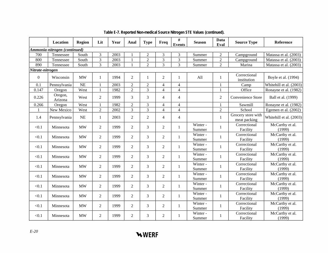
Table E-7. Reported Non-medical Source Nitrogen STE Values (continued).
Location Region Lit Year Anal Type Freq # Events Season Data
Eval Source Type Reference
Ammonia-nitrogen (continued) 700 Tennessee South 3 2003 1 2 3 3 Summer 2 Campground Matassa et al. (2003)800 Tennessee South 3 2003 1 2 3 3 Summer 2 Campground Matassa et al. (2003)890 Tennessee South 3 2003 1 2 3 3 Summer 2 Marina Matassa et al. (2003)
Nitrate-nitrogen
0 Wisconsin MW 1 1994 2 1 2 1 All 1 Correctional institution Boyle et al. (1994)
0.1 Pennsylvania NE 1 2003 2 2 4 4 1 Camp Whitehill et al. (2003)0.147 Oregon West 1 1982 2 3 4 4 1 Office Ronayne et al. (1982)
0.226 Oregon, Arizona West 2 1999 3 3 4 4 2 Convenience Store Ball et al. (1999)
0.266 Oregon West 1 1982 2 3 4 4 1 Sawmill Ronayne et al. (1982)1 New Mexico West 2 2002 3 3 4 4 2 School Egemen et al. (2002)
1.4 Pennsylvania NE 1 2003 2 2 4 4 1 Grocery store with meat packing Whitehill et al. (2003)
<0.1 Minnesota MW 2 1999 2 3 2 1 Winter - Summer 1 Correctional
Facility McCarthy et al.
(1999)
<0.1 Minnesota MW 2 1999 2 3 2 1 Winter - Summer 1 Correctional
Facility McCarthy et al.
(1999)
<0.1 Minnesota MW 2 1999 2 3 2 1 Winter - Summer 1 Correctional
Facility McCarthy et al.
(1999)
<0.1 Minnesota MW 2 1999 2 3 2 1 Winter - Summer 1 Correctional
Facility McCarthy et al.
(1999)
<0.1 Minnesota MW 2 1999 2 3 2 1 Winter - Summer 1 Correctional
Facility McCarthy et al.
(1999)
<0.1 Minnesota MW 2 1999 2 3 2 1 Winter - Summer 1 Correctional
Facility McCarthy et al.
(1999)
<0.1 Minnesota MW 2 1999 2 3 2 1 Winter - Summer 1 Correctional
Facility McCarthy et al.
(1999)
<0.1 Minnesota MW 2 1999 2 3 2 1 Winter - Summer 1 Correctional
Facility McCarthy et al.
(1999)
<0.1 Minnesota MW 2 1999 2 3 2 1 Winter - Summer 1 Correctional
Facility McCarthy et al.
(1999)
<0.1 Minnesota MW 2 1999 2 3 2 1 Winter - Summer 1 Correctional
Facility McCarthy et al.
(1999)
E-200

Table E-7. Reported Non-medical Source Nitrogen STE Values (continued).
Location Region Lit Year Anal Type Freq # Events Season Data
Eval Source Type Reference
Nitrate-nitrogen (continued)
<0.1 Minnesota MW 2 1999 2 3 2 1 Winter - Summer 1 Correctional
Facility McCarthy et al.
(1999)
<0.1 Minnesota MW 2 1999 2 3 2 1 Winter - Summer 1 Correctional
Facility McCarthy et al.
(1999)
<0.1 Minnesota MW 2 1999 2 3 2 1 Winter - Summer 1 Correctional
Facility McCarthy et al.
(1999)
<0.1 Minnesota MW 2 1999 2 3 2 1 Winter - Summer 1 Correctional
Facility McCarthy et al.
(1999)
<0.1 Minnesota MW 2 1999 2 3 2 1 Winter - Summer 1 Correctional
Facility McCarthy et al.
(1999)
<0.1 Minnesota MW 2 1999 2 3 2 1 Winter - Summer 1 Correctional
Facility McCarthy et al.
(1999)
<0.1 Minnesota MW 2 1999 2 3 2 1 Winter - Summer 1 Correctional
Facility McCarthy et al.
(1999)
<0.02 Oregon, Arizona West 2 1999 3 3 4 4 2 Camp Ball et al. (1999)
blank = information not provided
Influent Constituent Characteristics of the Modern Waste Stream from Single Sources E-211

Table E-8. Reported Medical Source Nitrogen STE Values.
Location Region Lit Year Anal Type Freq # Events Season Data
Eval Source Type Reference
Total nitrogen
28.3 Mass. NE 2 1999 2 2 3 2 All 1 Doctor Higgins and Groves (1999)
29 Mass. NE 2 1999 2 2 3 2 All 1 Nursing Home Higgins and Groves (1999)
32.4 Mass. NE 2 1999 2 2 3 2 All 1 Nursing Home Higgins and Groves (1999)
38.8 Mass. NE 2 1999 2 2 3 2 All 1 Assisted Living Facility
Higgins and Groves (1999)
41.2 Mass. NE 2 1999 2 2 3 2 All 1 Nursing Home Higgins and Groves (1999)
42.2 Mass. NE 2 1999 2 2 3 2 All 1 Veterinary/ Kennel
Higgins and Groves (1999)
49 Mass. NE 2 1999 2 2 3 2 All 1 Assisted Living Facility
Higgins and Groves (1999)
56.5 Mass. NE 2 1999 2 2 3 2 All 1 Veterinary/ Kennel
Higgins and Groves (1999)
57.5 Mass. NE 2 1999 2 2 3 2 All 1 Veterinary/ Kennel
Higgins and Groves (1999)
64 Mass. NE 2 1999 2 2 3 2 All 1 Assisted Living Facility
Higgins and Groves (1999)
105 Mass. NE 2 1999 2 2 3 2 All 1 Doctor Higgins and Groves (1999)
125 Mass. NE 2 1999 2 2 3 2 All 1 Doctor Higgins and Groves (1999)
blank = information not provided
E-222

Table E-9. Reported Municipal Source Nitrogen Values.
Total Nitrogen (mg-N/L) Sample Description Reference 23.1 Raw Wastewater Babcock et al. (2001) 30 Influent Yang et al. (2004) 36 Influent Bradstreet et al. (2002)
38.9 Influent Kwon et al. (2003) 50.8 Effluent Danielson (2006) 76 Influent Zheng et al. (2002) 105 Wastewater Characteristics Gale (2002) 109 Influent Zheng et al. (2002)
Table E-10. Other Reported Nitrogen Raw Wastewater and STE Values.
Average Value Constituent (units) Source Waste Stream Reference 30.3 Organic N (mg/L) Raw Single-source domestic Ziebell et al. (1974) 35.07 Organic N (mg/L) Raw Single-source domestic Hanson et al. (2002) 68.96 Organic N (mg/L) Raw Single-source domestic Hanson et al. (2002) 70.43 Organic N (mg/L) Raw Single-source domestic Hanson et al. (2002)
50 Organic N (mg/L) Raw Non-medical, Rest Area Restroom Pearson et al. (1987) 202 Organic N (mg/L) Raw Non-medical, RV Dump Pearson et al. (1987) 10 Organic N (mg/L) STE Single-source domestic Converse et al. (1994) 10 Organic N (mg/L) STE Single-source domestic Walker et al. (1973)
14.23 Organic N (mg/L) STE Single-source domestic Hanson et al. (2002) 15 Organic N (mg/L) STE Single-source domestic Rock et al. (1981) 15 Organic N (mg/L) STE Single-source domestic Walker et al. (1973) 15 Organic N (mg/L) STE Single-source domestic Walker et al. (1973) 15 Organic N (mg/L) STE Single-source domestic Walker et al. (1973) 16 Organic N (mg/L) STE Single-source domestic Ziebell et al. (1974)
30.4 Organic N (mg/L) STE Single-source domestic Harrison et al. (2000) 44.6 Organic N (mg/L) STE Single-source domestic Harrison et al. (2000) 105 Organic N (mg/L) STE Single-source domestic Harrison et al. (2000)
5 Organic N (mg/L) STE Multiple-source domestic Brandes et al. (1974) 6.83 Organic N (mg/L) STE Multiple-source domestic Brown et al. (1977) 11 Organic N (mg/L) STE Multiple-source domestic Converse et al. (1991)
0.02 NO2 (mg/L) STE Single-source domestic Ronayne et al. (1982) 0.02 NO2 (mg/L) STE Single-source domestic Ronayne et al. (1982)
Influent Constituent Characteristics of the Modern Waste Stream from Single Sources E-233

Table E-10. Other Reported Nitrogen Raw Wastewater and STE Values (continued).
Average Value Constituent (units) Source Waste Stream Reference 0.02 NO2 (mg/L) STE Single-source domestic Ronayne et al. (1982) 0.02 NO2 (mg/L) STE Single-source domestic Ronayne et al. (1982) 0.02 NO2 (mg/L) STE Single-source domestic Ronayne et al. (1982) 0.02 NO2 (mg/L) STE Single-source domestic Ronayne et al. (1982) 0.03 NO2 (mg/L) STE Single-source domestic Ronayne et al. (1982) 0.06 NO2 (mg/L) STE Single-source domestic Bruen and Piluk (1994) 0.04 NO2 (mg/L) STE Non-medical, sawmill Ronayne et al. (1982) 0.05 NO2 (mg/L) STE Non-medical, Office Ronayne et al. (1982) 0.05 NO2 (mg-N/L) Raw Single-source domestic Hanson et al. (2002)
0.0569 NO2 (mg-N/L) Raw Single-source domestic Hanson et al. (2002) 0.1125 NO2 (mg-N/L) Raw Single-source domestic Hanson et al. (2002) 0.05 NO2 (mg-N/L) STE Single-source domestic Hanson et al. (2002) 0.07 NO2 (mg-N/L) STE Multiple-source domestic Brandes et al. (1974) <.05 NO2 (mg-N/L) STE Multiple-source domestic Brown et al. (1977)
0 NO2 (mg-N/L) STE Non-medical, Camp Whitehill et al. (2003) 0.1 NO2 (mg-N/L) STE Non-medical, Grocery Store with Meat Packing Whitehill et al. (2003) 0.1 NOx (mg/L) Raw Single-source domestic Thiruvenkatachari (1976) 1.8 NOx (mg/L) Raw Single-source domestic Ziebell et al. (1974)
0.03 NOx (mg/L) Raw Non-medical, Min. Security Correctional Inst. Anderson et al. (1998) 0.02 NOx (mg/L) STE Single-source domestic Thiruvenkatachari (1976) 0.04 NOx (mg/L) STE Single-source domestic Roy et al. (1998) 0.08 NOx (mg/L) STE Single-source domestic Sherman and Anderson (1991)
0.0837 NOx (mg/L) STE Single-source domestic Engeset and Seabloom (1978) 0.3 NOx (mg/L) STE Single-source domestic Sauer et al. (1976)
0.35 NOx (mg/L) STE Single-source domestic Otis et al. (1974a) 0.46 NOx (mg/L) STE Single-source domestic Otis et al. (1974a) 0.56 NOx (mg/L) STE Single-source domestic Otis and Boyle (1976) 0.6 NOx (mg/L) STE Single-source domestic Effert et al. (1984) 0.6 NOx (mg/L) STE Single-source domestic Ziebell et al. (1974)
0.68 NOx (mg/L) STE Single-source domestic Otis et al. (1974a) 0.83 NOx (mg/L) STE Single-source domestic Otis et al. (1974a) <.5 NOx (mg/L) STE Single-source domestic Roy et al. (1998)
E-244

Table E-10. Other Reported Nitrogen Raw Wastewater and STE Values (continued).
Average Value Constituent (units) Source Waste Stream Reference 0.05 NOx (mg/L) STE Non-medical, Camp Site Ptacek (1998) 0.073 NOx (mg/L) STE Non-medical, Residential/Health Clinic/Casino Martinson et al. (2001) 0.2 NOx (mg/L) STE Non-medical, Dairy Farm Christopherson et al. (2004) 0.3 NOx (mg/L) STE Non-medical, Dairy Farm Christopherson et al. (2004) 0.4 NOx (mg/L) STE Non-medical, Dairy Farm Christopherson et al. (2004) 0.7 NOx (mg/L) STE Non-medical, Dairy Farm Christopherson et al. (2004) 1 NOx (mg/L) STE Non-medical, Dairy Farm Christopherson et al. (2004)
Table E-11. Reported Single Source Domestic Total Phosphorus Raw Wastewater Values.
Total P Location Region Lit Year Anal Type Freq # Events Season Data
Eval Reference
13.0 Kentucky South 1 1967 2 1 4 4 1 Watson et al. (1967) 15.3 Kentucky South 1 1967 2 1 4 4 1 Watson et al. (1967) 16.6 Kentucky South 1 1967 2 1 4 4 1 Watson et al. (1967) 19 California West 2 2002 3 2 4 2 2 Edvardsson (2002) 19 California West 2 2000 3 1 1 1 Summer 1 Edvardsson and Spears (2000)
21.2 Kentucky South 1 1967 2 1 4 4 1 Watson et al. (1967) 22.8 Kentucky South 1 1967 2 1 4 4 1 Watson et al. (1967) 25.8 Kentucky South 1 1967 2 1 4 4 1 Watson et al. (1967)
blank = information not provided
Table E-12. Reported Multiple Source Domestic Total Phosphorus Raw Wastewater Values.
Total P Location Region Lit Year Anal Type Freq # Events Season Data
Eval Reference
13 Arizona West 1 1989 2 1 1 2 Fall 1 Anderson and Siegrist (1989) 26 Arizona West 1 1989 2 1 1 2 Fall 1 Anderson and Siegrist (1989) 57 Wisconsin MW 2 1978 2 3 4 4 1 Siegrist (1978)
blank = information not provided
Influent Constituent Characteristics of the Modern Waste Stream from Single Sources E-255
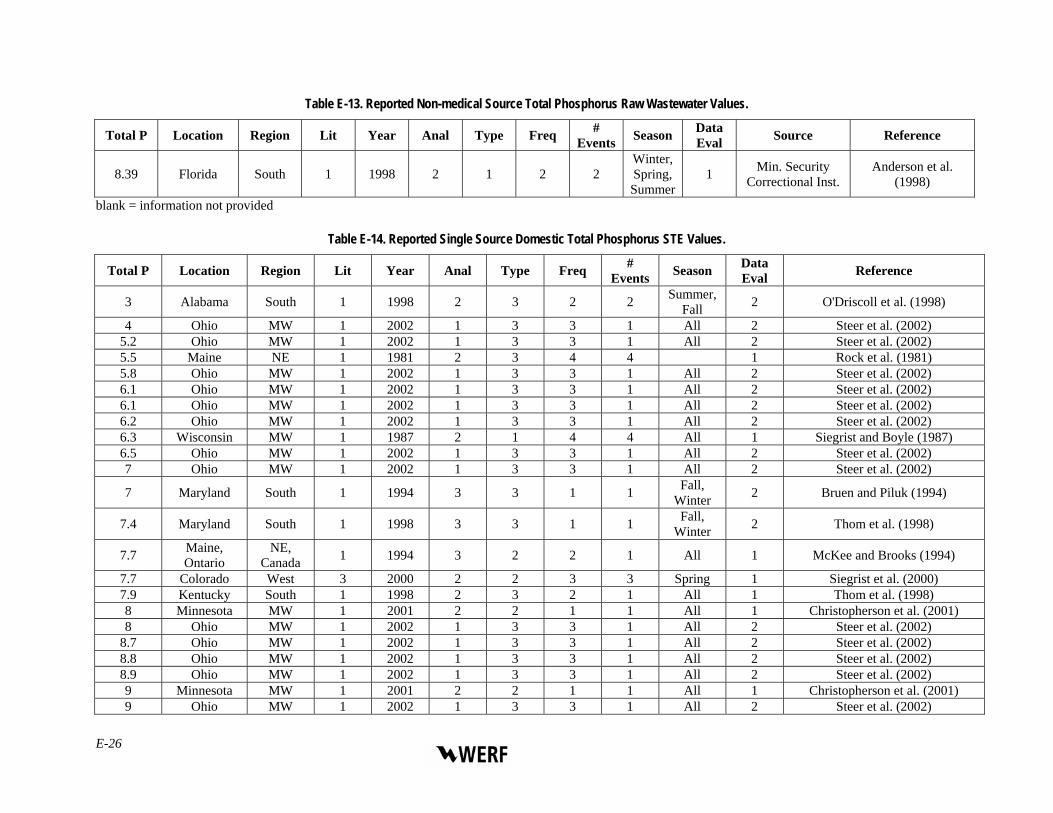
Table E-13. Reported Non-medical Source Total Phosphorus Raw Wastewater Values.
Total P Location Region Lit Year Anal Type Freq # Events Season Data
Eval Source Reference
8.39 Florida South 1 1998 2 1 2 2 Winter, Spring, Summer
1 Min. Security Correctional Inst.
Anderson et al. (1998)
blank = information not provided
Table E-14. Reported Single Source Domestic Total Phosphorus STE Values.
Total P Location Region Lit Year Anal Type Freq # Events Season Data
Eval Reference
3 Alabama South 1 1998 2 3 2 2 Summer, Fall 2 O'Driscoll et al. (1998)
4 Ohio MW 1 2002 1 3 3 1 All 2 Steer et al. (2002) 5.2 Ohio MW 1 2002 1 3 3 1 All 2 Steer et al. (2002) 5.5 Maine NE 1 1981 2 3 4 4 1 Rock et al. (1981) 5.8 Ohio MW 1 2002 1 3 3 1 All 2 Steer et al. (2002) 6.1 Ohio MW 1 2002 1 3 3 1 All 2 Steer et al. (2002) 6.1 Ohio MW 1 2002 1 3 3 1 All 2 Steer et al. (2002) 6.2 Ohio MW 1 2002 1 3 3 1 All 2 Steer et al. (2002) 6.3 Wisconsin MW 1 1987 2 1 4 4 All 1 Siegrist and Boyle (1987) 6.5 Ohio MW 1 2002 1 3 3 1 All 2 Steer et al. (2002) 7 Ohio MW 1 2002 1 3 3 1 All 2 Steer et al. (2002)
7 Maryland South 1 1994 3 3 1 1 Fall, Winter 2 Bruen and Piluk (1994)
7.4 Maryland South 1 1998 3 3 1 1 Fall, Winter 2 Thom et al. (1998)
7.7 Maine, Ontario
NE, Canada 1 1994 3 2 2 1 All 1 McKee and Brooks (1994)
7.7 Colorado West 3 2000 2 2 3 3 Spring 1 Siegrist et al. (2000) 7.9 Kentucky South 1 1998 2 3 2 1 All 1 Thom et al. (1998) 8 Minnesota MW 1 2001 2 2 1 1 All 1 Christopherson et al. (2001) 8 Ohio MW 1 2002 1 3 3 1 All 2 Steer et al. (2002)
8.7 Ohio MW 1 2002 1 3 3 1 All 2 Steer et al. (2002) 8.8 Ohio MW 1 2002 1 3 3 1 All 2 Steer et al. (2002) 8.9 Ohio MW 1 2002 1 3 3 1 All 2 Steer et al. (2002) 9 Minnesota MW 1 2001 2 2 1 1 All 1 Christopherson et al. (2001) 9 Ohio MW 1 2002 1 3 3 1 All 2 Steer et al. (2002)
E-26

Table E-14. Reported Single Source Domestic Total Phosphorus STE Values (continued).
Total P Location Region Lit Year Anal Type Freq #
Events Season Data Eval Reference
9.1 Ohio MW 1 2002 1 3 3 1 All 2 Steer et al. (2002) 9.3 Ohio MW 1 1998 1 3 3 1 All 2 Thom et al. (1998) 10 Oregon West 2 2003 2 3 4 3 1 Rich et al. (2003) 10 Oregon West 2 2003 2 3 4 3 1 Rich et al. (2003) 10 Colorado West 3 2000 2 2 3 3 Spring 1 Siegrist et al. (2000)
10.3 South Wales Australia 1 2004 2 2 4 2 All 1 Patterson (2004) 10.8 California West 1980 3 3 4 2 Winter 2 Baker (1980) 10.9 Ohio MW 1 2002 1 3 3 1 All 2 Steer et al. (2002)
11 Florida South 1 1991 2 2 1 1 Fall - Spring 1 Sherman and Anderson (1991)
11 Wisconsin MW 1 1974 2 1 2 1 All 1 Otis et al. (1974a) 11 Oregon West 3 2005 2 2 2,3 1 All 1 Rich (2006)
11.3 Ohio MW 1 2002 1 3 3 1 All 2 Steer et al. (2002) 11.6 Wisconsin MW 1 1974 2 1 2 1 All 1 Otis et al. (1974a) 12.3 Ohio MW 1 2002 1 3 3 1 All 2 Steer et al. (2002) 12.3 Wisconsin MW 1 1974 2 1 2 1 All 1 Otis et al. (1974a)
12.3 Washington West 2 1981 3 3 2 1 Fall - Spring 1 Seabloom et al. (1981)
14.1 Wisconsin MW 1 1974 2 1 2 1 All 1 Otis et al. (1974a)
14.3 Washington West 2 1981 3 3 2 1 Fall - Spring 1 Seabloom et al. (1981)
16.9 Ohio MW 1 2002 1 3 3 1 All 2 Steer et al. (2002)
17.3 Washington West 2 1981 3 3 2 1 Fall - Spring 1 Seabloom et al. (1981)
18.4 Wisconsin MW 1 1981 2 1 4 4 1 Hargett et al. (1981) 19.5 Ohio MW 1 1984 2 1 1 1 All 1 Effert et al. (1984) 23 3 1977 3 3 4 4 2 Siegrist (1977)
24.7 Washington West 2 1981 3 3 2 1 Fall - Spring 1 Seabloom et al. (1981)
26.2 Washington West 2 1978 1 3 2 1 Summer, Fall 1 Engeset and Seabloom (1978)
27.4 Ohio MW 1 2002 1 3 3 1 All 2 Steer et al. (2002)
34.75 Alabama South 1 1998 2 3 2 2 Summer, Fall 2 O'Driscoll et al. (1998)
39.5 Maine, Ontario NE, Canada 1 1994 3 2 2 1 All 1 McKee and Brooks (1994)
Influent Constituent Characteristics of the Modern Waste Stream from Single Sources E-27

blank = information not provided Table E-15. Reported Multiple Source Domestic Total Phosphorus STE Values.
Total P Location Region Lit Year Anal Type Freq # Events Season Data
Eval Reference
5 Wisconsin MW 2 1991 3 2 4 4 1 Converse et al. (1991) 5.4 Minnesota MW 1 2001 2 3 2 1 All 1 Henneck et al. (2001)
6.02 1985 3 3 4 4 2 Swed (1985) 7.87 Norway Norway 1 1991 2 3 1 2 1 Siegrist et al. (1991) 7.9 Minnesota MW 1 2001 2 3 2 1 All 1 Henneck et al. (2001) 10 Ontario Canada 1 1974 3 3 1 1 ALL 2 Brandes et al. (1974)
blank = information not provided
Table E-16. Reported Food Source Total Phosphorus STE Values.
Total P Location Region Lit Year Anal Type Freq # Events Season Data
Eval Reference
13.5 Maine, Ontario
NE, Canada 1 1994 3 2 2 1 All 1 McKee and Brooks (1994)
14 Wisconsin MW 1 1984 2 2 4 4 2 Siegrist et al. (1984b) 15 Wisconsin MW 1 1984 2 2 4 4 2 Siegrist et al. (1984b) 19 Wisconsin MW 1 1984 2 2 4 4 2 Siegrist et al. (1984b) 23 Wisconsin MW 1 1984 2 2 4 4 2 Siegrist et al. (1984b) 24 Wisconsin MW 1 1984 2 2 4 4 2 Siegrist et al. (1984b) 28 Wisconsin MW 1 1984 2 2 4 4 2 Siegrist et al. (1984b)
blank = information not provided
E-288

Table E-17. Reported Non-medical Source Total Phosphorus STE Values.
Year Anal Type Freq # Events
Data Eval Source Reference Total P Location Region Lit Season
Maine, Ontario
NE, Canada 1 1994 3 McKee and Brooks
(1994) 4.1 2 2 1 All 1 School
5.5 Maine, Ontario
NE, Canada 1 1994 3 2 2 1 All 1 Shopping Plaza McKee and Brooks
(1994)
5.8 Maine, Ontario
NE, Canada All 1 School McKee and Brooks
(1994) 1 1994 3 2 2 1
McKee and Brooks (1994)
Maine, Ontario
NE, Canada 1 1994 3 2 2 1 All 1 School 5.9
6.1 Maine, Ontario
NE, Canada 1 1994 3 2 2 1 All 1 School McKee and Brooks
(1994) 6.6 California West 2 1980 3 3 4 2 Winter 2 Ski area Baker (1980)
Maine, Ontario
NE, Canada 1 1994 3 McKee and Brooks
(1994) 6.9 2 2 1 All 1 School
6.9 Tennessee South 3 2003 1 2 3 3 Summer 2 Marina Matassa et al. (2003)
7 Wisconsin All 1 Correctional institution Boyle et al. (1994) MW 1 1994 2 1 2 1
10 Wisconsin MW 1 1984 2 2 4 4 2 Golf club Siegrist et al. (1984b)
11 Minnesota MW 2 1999 2 3 2 1 Winter - Summer 1 Correctional
Facility McCarthy et al.
(1999)
11 Minnesota MW 2 1999 2 3 2 1 Winter - Summer 1 Correctional
Facility McCarthy et al.
(1999)
11 Minnesota MW 2 1999 2 3 2 1 Winter - Summer 1 Correctional
Facility McCarthy et al.
(1999)
11 Minnesota MW 2 1999 2 3 2 1 Winter - Summer 1 Correctional
Facility McCarthy et al.
(1999)
11 Minnesota MW 2 1999 2 3 2 1 Winter - Summer 1 Correctional
Facility McCarthy et al.
(1999)
12 Minnesota MW 2 1999 2 3 2 1 Winter - Summer 1 Correctional
Facility McCarthy et al.
(1999)
12 Minnesota MW 2 1999 2 3 2 1 Winter - Summer 1 Correctional
Facility McCarthy et al.
(1999)
Influent Constituent Characteristics of the Modern Waste Stream from Single Sources E-299

Table E-17. Reported Non-medical Source Total Phosphorus STE Values (continued).
Total P Location Region Lit Year Anal Type Freq # Events Season Data
Eval Source Reference
12 Minnesota MW 2 1999 2 3 2 1 Winter - Summer 1 Correctional
Facility McCarthy et al.
(1999)
12 Minnesota MW 2 1999 2 3 2 1 Winter - Summer 1 Correctional
Facility McCarthy et al.
(1999)
13 Minnesota MW 1 2001 2 3 2 1 All 1 Correctional Facility
Henneck et al. (2001)
13 Wisconsin MW 1 1984 2 2 4 4 2 Golf club Siegrist et al. (1984b)
15 Minnesota MW 2 1999 2 3 2 1 Winter - Summer 1 Correctional
Facility McCarthy et al.
(1999)
15 Minnesota MW 2 1999 2 3 2 1 Winter - Summer 1 Correctional
Facility McCarthy et al.
(1999)
15 Tennessee South 3 2003 1 2 3 3 Summer 2 Marina Matassa et al. (2003)
16 Minnesota MW 2 1999 2 3 2 1 Winter - Summer 1 Correctional
Facility McCarthy et al.
(1999)
16 Minnesota MW 2 1999 2 3 2 1 Winter - Summer 1 Correctional
Facility McCarthy et al.
(1999)
16 Minnesota MW 2 1999 2 3 2 1 Winter - Summer 1 Correctional
Facility McCarthy et al.
(1999)
16 Minnesota MW 2 1999 2 3 2 1 Winter - Summer 1 Correctional
Facility McCarthy et al.
(1999)
16 Minnesota MW 2 1999 2 3 2 1 Winter - Summer 1 Correctional
Facility McCarthy et al.
(1999)
17 Wisconsin MW 1 1984 2 2 4 4 2 Golf club Siegrist et al. (1984b)
18 Tennessee South 3 2003 1 2 3 3 Summer 2 Marina Matassa et al. (2003)
20 Minnesota MW 2 1999 2 3 2 1 Winter - Summer 1 Correctional
Facility McCarthy et al.
(1999)
20 Wisconsin MW 1 1984 2 2 4 4 2 Motel Siegrist et al. (1984b)
31 Tennessee South 3 2003 1 2 3 3 Summer 2 Marina Matassa et al. (2003)
33 Tennessee South 3 2003 1 2 3 3 Summer 2 Marina Matassa et al. (2003)
E-300

Table E-17. Reported Non-medical Source Total Phosphorus STE Values (continued).
Total P Location Region Lit Year Anal Type Freq # Events Season Data
Eval Source Reference
37 Tennessee South 3 2003 1 2 3 3 Summer 2 Marina Matassa et al. (2003)
42 Tennessee South 3 2003 1 2 3 3 Summer 2 Marina Matassa et al. (2003)
44 Tennessee South 3 2003 1 2 3 3 Summer 2 Campground Matassa et al. (2003)
67 Tennessee South 3 2003 1 2 3 3 Summer 2 Campground Matassa et al. (2003)
78 Tennessee South 3 2003 1 2 3 3 Summer 2 Campground Matassa et al. (2003)
96 Tennessee South 3 2003 1 2 3 3 Summer 2 Marina Matassa et al. (2003)
100 Tennessee South 3 2003 1 2 3 3 Summer 2 Campground Matassa et al. (2003)
blank = information not provided
Influent Constituent Characteristics of the Modern Waste Stream from Single Sources E-311

Table E-18. Reported Municipal Source Total Phosphorus \Values.
Total Phosphorus (mg-P/L) Sample Description Reference 3.1 Influent Sadler et al. (2002) 3.2 Influent Rock and Capron (2002) 3.8 Domestic Sewage Shin et al. (2002) 3.8 Influent Yang et al. (2004) 4.1 Influent Sadler et al. (2002) 4.6 Raw Wastewater Babcock et al. (2001) 4.9 Influent Sadler et al. (2002) 4.9 Domestic Sewage Shin et al. (2002) 5.3 Influent Stephens et al. (2004) 5.3 Influent Insel et al. (2003) 5.3 Influent Zhao et al. (2002) 5.7 After Screen Curto et al. (2002) 5.8 Influent Zheng et al. (2002) 6.1 Influent Stephens et al. (2004) 6.3 Influent Kwon et al. (2003) 6.5 Influent Stephens et al. (2004) 6.7 Influent Sadler et al. (2002) 7 Typical Raw Wastewater Lorenz et al. (2002)
7.1 Raw Wastewater Johnson et al. (2002) 7.4 Influent Randall et al. (2000) 7.5 Influent Sadler et al. (2002) 7.7 Typical Concentration for Wastewater Chen et al. (2002) 7.8 Influent Zheng et al. (2002) 8.5 Influent Stephens et al. (2004)
8.54 Raw Wastewater Xingcan et al. (2001) 8.7 Raw Wastewater Jones and Takacs (2004) 9.1 Raw Wastewater Crawford et al. (2000) 9.3 After Screen Curto et al. (2002) 9.8 After Screen Curto et al. (2002)
10.1 Before Pump Curto et al. (2002) 12.3 Before Primary Settler Curto et al. (2002) 13.5 Wastewater Characteristics Gale (2002) 14 Influent Stephens et al. (2004) 15 Influent Magro et al. (2003) 40 Influent Barnard et al. (2004)
E-322

Table E-19. Other Reported Phosphorus Raw Wastewater and STE Values.
Average Value Constituent (units) Source Waste Stream Reference 1.9 Total Phosphate (mg-P/L) STE Single-source domestic Lindbo and MacConnell (2001)
3.15 Total Phosphate (mg-P/L) STE Single-source domestic Huang et al. (1994) 4.4 Total Phosphate (mg-P/L) STE Single-source domestic Lindbo and MacConnell (2001) 6.4 Total Phosphate (mg-P/L) STE Single-source domestic Reneau et al. (2001) 9 Total Phosphate (mg-P/L) STE Single-source domestic Reneau et al. (2001)
10.9 Total Phosphate (mg-P/L) STE Single-source domestic Viraraghavan and Rana (1991) 8.18 Total Phosphate (mg-P/L) STE Multiple-source domestic Brown et al. (1977) 3.36 Phosphate (mg/L) STE Single-source domestic Duncan et al. (1994) 50 Phosphate (mg-P/L) Raw Non-medical, Rest Area Restroom Pearson et al. (1987)
114 Phosphate (mg-P/L) Raw Non-medical, RV Dump Pearson et al. (1987) 8.9 Phosphate (mg-P/L) STE Single-source domestic Wilhelm et al. (1996) 9 Phosphate (mg-P/L) STE Single-source domestic Robertson and Blowes (1995)
13.1 Phosphate (mg-P/L) STE Single-source domestic Wilhelm et al. (1996) 9 Phosphate (mg-P/L) STE Non-medical, Elementary School Harmon et al. (1996)
14 Orthophosphate (mg/L) Raw Single-source domestic Thiruvenkatachari (1976) 3.8 Orthophosphate (mg/L) STE Single-source domestic Seabloom et al. (1981) 4.7 Orthophosphate (mg/L) STE Single-source domestic Seabloom et al. (1981)
10.2 Orthophosphate (mg/L) STE Single-source domestic Seabloom et al. (1981) 10.5 Orthophosphate (mg/L) STE Single-source domestic Thiruvenkatachari (1976) 10.9 Orthophosphate (mg/L) STE Single-source domestic Sauer et al. (1976) 11.5 Orthophosphate (mg/L) STE Single-source domestic Otis and Boyle (1976) 14.2 Orthophosphate (mg/L) STE Single-source domestic Seabloom et al. (1981) 22 Orthophosphate (mg/L) STE Single-source domestic Seabloom et al. (1981) 1.5 Orthophosphorus (mg-P/L) STE Single-source domestic Lindbo and MacConnell (2001) 3.7 Orthophosphorus (mg-P/L) STE Single-source domestic Lindbo and MacConnell (2001)
6.36 Orthophosphorus (mg-P/L) STE Single-source domestic Hanson et al. (2002) 8 Orthophosphorus (mg-P/L) STE Single-source domestic Sauer and Boyle (1977)
10 Orthophosphorus (mg-P/L) STE Single-source domestic Sauer and Boyle (1977) 10.1 Orthophosphorus (mg-P/L) STE Single-source domestic Otis et al. (1974a) 10.5 Orthophosphorus (mg-P/L) STE Single-source domestic Otis et al. (1974a) 10.8 Orthophosphorus (mg-P/L) STE Single-source domestic Otis et al. (1974a) 11.5 Orthophosphorus (mg-P/L) STE Single-source domestic Ziebell et al. (1974)
Influent Constituent Characteristics of the Modern Waste Stream from Single Sources E-331

E-34
Table E-19. Other Reported Phosphorus Raw Wastewater and STE Values (continued).
Average Value Constituent (units) Source Waste Stream Reference 13.6 Orthophosphorus (mg-P/L) STE Single-source domestic Otis et al. (1974a) 13.7 Orthophosphorus (mg-P/L) STE Single-source domestic Engeset and Seabloom (1978) 15 Orthophosphorus (mg-P/L) STE Single-source domestic Sauer and Boyle (1977)
15.7 Orthophosphorus (mg-P/L) STE Single-source domestic Wolf et al. (1998) 36 Orthophosphorus (mg-P/L) STE Non-medical, Lab (simulated household) Siegrist (1978) 3.6 Soluble P (mg/L) STE Single-source domestic Thom et al. (1998) 5.8 Soluble P (mg/L) STE Single-source domestic Thom et al. (1998) 7.8 Soluble P (mg/L) STE Single-source domestic Thom et al. (1998) 6.2 Soluble P (mg/L) STE Multiple-source domestic Cogger et al. (1988) 3.1 Organic P (mg/L) STE Single-source domestic Ziebell et al. (1974) 12 Reactive Phosphorus (mg/L) Raw Single-source domestic Edvardsson and Spears (2000)

APPENDIX F
COMPLETE LISTING OF REPORTED FECAL COLIFORM VALUES
Influent Constituent Characteristics of the Modern Waste Stream from Single Sources F-1

Tables F-1 through F-5 summarize the reported values and the data qualifiers used. The following key should be used to interpret the data qualifier information within the tables. A more detailed description of the data qualifiers can be found in the report, Section 3.4.1.
Location = state where the study was conducted
Region = location of the study based on US Census defined regions MW = Midwest: IL, IN, IA, KS, MI, MN, MO, NE, ND, OH, SD, and WI NE = Northeast: CT, ME, MA, NH, NJ, NY, PA, RI, VT South: AL, AR, DE, DC, FL, GA, KY, LA, MD, MS, NC, OK, SC, TN, TX, VA, and WV West: AK, AZ, CA, CO, HI, ID, MT, NV, NM, OR, UT, WA, and WY
Lit = literature source 1 – publicly available and published in a peer reviewed journal 2 – publicly available and published in conference proceedings or project report 3 – unpublished; information obtained directly from researcher and is not publicly available
Year = year the study was conducted
Anal = analytical method used 1 – detailed methods used = specified which approved method was used (e.g., APHA 4500-N B). 2 – standard methods = specified use of approved methods (e.g., APHA). 3 – no methods = did not specify which method was used
Type = sampling technique used 1 – composite sample collected 2 – grab sample collected 3 – unknown; type of sample collected was not specified
Freq = frequency of sample collection 1 – at least weekly 2 – bi-weekly to monthly 3 – less than one time per month 4 – unknown
# Events = number of sampling events 1 – more than 12 sampling events reported 2 – between 3 and 12 sampling events reported 3 – less than 3 sampling events reported 4 – unknown; number of sampling events not reported
Season = time of year when study was conducted Spring (Mar-May) Summer (Jun-Aug) Fall (Sept-Nov) Winter (Dec-Feb) All (Jan-Dec)
Data Eval = data evaluation 1 –more than a single average value reported (e.g., descriptive statistics provided) 2 – only the average value reported for each constituent
F-2

Table F-1. Reported Single-Source Domestic Fecal Coliform Raw Wastewater Values.
Fecal Coliform Location Region Lit Year Anal Type Freq #
Events Season Data Eval Reference
3.0E+04 1 1976 3 3 4 4 2 Thiruvenkatachari (1976) 4.6E+05 New Mexico West 1 2002 3 1 2 1 All 1 Hanson et al. (2002) 4.9E+05 California West 2 2000 3 1 1 1 Summer 1 Edvardsson and Spears (2000) 6.0E+05 New Mexico West 1 2002 3 1 2 1 All 1 Hanson et al. (2002) 7.4E+06 New Mexico West 1 2002 3 1 2 1 All 1 Hanson et al. (2002)
blank = information not provided
Table F-2. Reported Single-Source Domestic Fecal Coliform STE Values.
Fecal Coliform Location Region Lit Year Anal Type Freq #
Events Season Data Eval Reference
1.9E+03 Ohio MW 1 2002 1 3 3 1 All 2 Steer et al. (2002)
3.1E+03 Arkansas South 1 1998 2 2 2 1 Fall - Spring 1 Wolf et al. (1998)
4.2E+03 1 1976 3 3 4 4 2 Otis and Boyle (1976) 1.1E+04 Ohio MW 1 2002 1 3 3 1 All 2 Steer et al. (2002) 1.1E+04 Ohio MW 1 2002 1 3 3 1 All 2 Steer et al. (2002) 1.7E+04 Ohio MW 1 2002 1 3 3 1 All 2 Steer et al. (2002) 1.7E+04 Ohio MW 1 2002 1 3 3 1 All 2 Steer et al. (2002) 2.0E+04 Ohio MW 1 2002 1 3 3 1 All 2 Steer et al. (2002) 2.7E+04 Virginia South 1 2001 2 2 4 4 2 Reneau et al. (2001) 2.8E+04 Ohio MW 1 2002 1 3 3 1 All 2 Steer et al. (2002) 3.8E+04 Ohio MW 1 2002 1 3 3 1 All 2 Steer et al. (2002) 6.6E+04 Ohio MW 1 2002 1 3 3 1 All 2 Steer et al. (2002) 7.0E+04 Oregon West 1 1982 2 3 4 4 1 Ronayne et al. (1982)
7.1E+04 Washington West 2 1981 3 3 2 1 Fall - Spring 1 Seabloom et al. (1981)
7.3E+04 New Mexico West 1 2002 3 1 2 1 All 1 Hanson et al. (2002) 7.8E+04 Ohio MW 1 2002 1 3 3 1 All 2 Steer et al. (2002) 8.0E+04 Oregon West 1 1982 2 3 4 4 1 Ronayne et al. (1982) 8.1E+04 Oregon West 1 1982 2 3 4 4 1 Ronayne et al. (1982) 8.8E+04 Rhode Island NE 2 1999 2 2 2 1 Summer 2 Sykes et al. (1999) 8.8E+04 Ohio MW 1 2002 1 3 3 1 All 2 Steer et al. (2002)
Influent Constituent Characteristics of the Modern Waste Stream from Single Sources F-3

Table F-2. Reported Single-Source Domestic Fecal Coliform STE Values (continued).
Fecal Coliform Location Region Lit Year Anal Type Freq #
Events Season Data Eval Reference
1.0E+05 Virginia South 1 2001 2 2 4 4 2 Reneau et al. (2001) 1.1E+05 Oregon West 1 1982 2 3 4 4 1 Ronayne et al. (1982) 1.1E+05 California West 1 1994 2 2 4 4 1 Cagle and Johnson (1994) 1.2E+05 Ohio MW 1 2002 1 3 3 1 All 2 Steer et al. (2002) 1.2E+05 Montreal Canada 1 1998 3 3 2 1 All 2 Roy et al. (1998)
1.5E+05 North Carolina South 1 2001 2 3 2 1 All 2 Lindbo and MacConnell (2001)
1.6E+05 1 1976 3 3 4 4 2 Thiruvenkatachari (1976) 1.8E+05 Saskatchewan Canada 1 1991 2 2 4 4 1 Viraraghavan and Rana (1991)
1.9E+05 South Wales, Australia Australia 1 2004 2 2 4 2 All 1 Patterson (2004)
1.9E+05 Rhode Island NE 2 1999 2 2 2 1 Summer 2 Sykes et al. (1999) 2.2E+05 Ohio MW 1 1984 2 1 1 1 All 1 Effert et al. (1984)
2.2E+05 Washington West 2 1981 3 3 2 1 Fall - Spring 1 Seabloom et al. (1981)
2.5E+05 North Carolina South 1 2001 2 3 2 1 All 2 Lindbo and MacConnell (2001)
2.5E+05 Oregon West 2 2003 2 3 4 3 1 Rich et al. (2003) 2.8E+05 Rhode Island NE 2 1999 2 2 2 1 Summer 2 Sykes et al. (1999) 2.9E+05 Rhode Island NE 2 1999 2 2 2 1 Winter 2 Sykes et al. (1999)
3.1E+05 Washington West 2 1978 1 3 2 1 Summer, Fall 1 Engeset and Seabloom (1978)
3.2E+05 Oregon West 2 2003 2 3 4 3 1 Rich et al. (2003)
4.3E+05 Alabama South 1 1998 2 3 2 2 Summer, Fall 2 O'Driscoll et al. (1998)
4.4E+05 Maryland South 1 1994 3 3 1 1 Fall, Winter 2 Bruen and Piluk (1994)
4.6E+05 Missouri MW 1 1998 2 3 2 1 All 2 Sievers (1998) 4.9E+05 Rhode Island NE 1 2001 2 3 2 2 All 1 Bohrer and Converse (2001) 4.9E+05 Minnesota MW 1 2001 2 2 1 1 All 1 Christopherson et al. (2001) 5.2E+05 Alabama South 1 1998 3 3 4 4 1 White and Shirk (1998) 5.4E+05 Oregon West 1 1982 2 3 4 4 1 Ronayne et al. (1982) 5.4E+05 1 1976 3 3 4 4 2 Sauer et al. (1976)
F-4

Table F-2. Reported Single-Source Domestic Fecal Coliform STE Values (continued).
Fecal Coliform Location Region Lit Year Anal Type Freq #
Events Season Data Eval Reference
6.0E+05 Wisconsin MW 2 1999 1 2 4 2 Winter - Summer 1 Converse and Converse (1999)
6.3E+05 Minnesota MW 1 2001 2 2 1 1 All 1 Christopherson et al. (2001)
6.4E+05 Virginia South 1 1994 1 3 2 2 Fall - Spring 2 Huang et al. (1994)
6.7E+05 Alabama South 1 1998 2 3 2 2 Summer, Fall 2 O'Driscoll et al. (1998)
9.0E+05 Wisconsin MW 1 1998 1 2 4 1 Converse and Converse (1998) 1.0E+06 Oregon West 1 1982 2 3 4 4 1 Ronayne et al. (1982) 1.7E+06 Rhode Island NE 2 1999 2 2 2 1 Winter 2 Sykes et al. (1999)
2.0E+06 Washington West 2 1981 3 3 2 1 Fall - Spring 1 Seabloom et al. (1981)
2.1E+06 Washington West 2 1981 3 3 2 1 Fall - Spring 1 Seabloom et al. (1981)
2.3E+06 Rhode Island NE 2 1999 2 2 2 1 Winter 2 Sykes et al. (1999) 2.4E+06 Rhode Island NE 1 1998 2 2 2 1 Winter 2 Thom et al. (1998) 2.4E+06 Rhode Island NE 2 2002 2 3 2 3 All 1 Loomis et al. (2002) 3.1E+06 Wisconsin MW 1 1994 2 2 4 3 1 Converse et al. (1994) 4.0E+06 Colorado West 3 2000 2 2 3 3 Spring 1 Siegrist et al. (2000) 1.3E+07 Colorado West 3 2000 2 2 3 3 Spring 1 Siegrist et al. (2000) 1.5E+07 Oregon West 3 2005 2 2 2,3 1 All 1 Rich (2006) 2.5E+07 Wisconsin MW 1 2000 2 2 4 3 1 Harrison et al. (2000) 6.9E+07 Kentucky South 1 1998 2 3 2 1 All 1 Thom et al. (1998) 8.9E+07 Kentucky South 1 2000 2 3 2 1 1 Harrison et al. (2000) 1.2E+08 Washington West 1 2000 2 3 4 4 2 Harrison et al. (2000) 1.3E+08 Washington West 1 1998 2 3 4 4 2 Thom et al. (1998)
blank = information not provided
Influent Constituent Characteristics of the Modern Waste Stream from Single Sources F--5
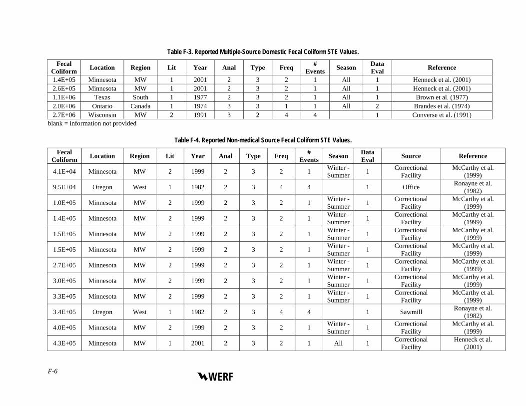
Table F-3. Reported Multiple-Source Domestic Fecal Coliform STE Values.
Fecal Coliform Location Region Lit Year Anal Type Freq #
Events Season Data Eval Reference
1.4E+05 Minnesota MW 1 2001 2 3 2 1 All 1 Henneck et al. (2001) 2.6E+05 Minnesota MW 1 2001 2 3 2 1 All 1 Henneck et al. (2001) 1.1E+06 Texas South 1 1977 2 3 2 1 All 1 Brown et al. (1977) 2.0E+06 Ontario Canada 1 1974 3 3 1 1 All 2 Brandes et al. (1974) 2.7E+06 Wisconsin MW 2 1991 3 2 4 4 1 Converse et al. (1991)
blank = information not provided
Table F-4. Reported Non-medical Source Fecal Coliform STE Values.
Fecal Coliform Location Region Lit Year Anal Type Freq #
Events Season Data Eval Source Reference
4.1E+04 Minnesota MW 2 1999 2 3 2 1 Winter - Summer 1 Correctional
Facility McCarthy et al.
(1999)
9.5E+04 Oregon West 1 1982 2 3 4 4 1 Office Ronayne et al. (1982)
1.0E+05 Minnesota MW 2 1999 2 3 2 1 Winter - Summer 1 Correctional
Facility McCarthy et al.
(1999)
1.4E+05 Minnesota MW 2 1999 2 3 2 1 Winter - Summer 1 Correctional
Facility McCarthy et al.
(1999)
1.5E+05 Minnesota MW 2 1999 2 3 2 1 Winter - Summer 1 Correctional
Facility McCarthy et al.
(1999)
1.5E+05 Minnesota MW 2 1999 2 3 2 1 Winter - Summer 1 Correctional
Facility McCarthy et al.
(1999)
2.7E+05 Minnesota MW 2 1999 2 3 2 1 Winter - Summer 1 Correctional
Facility McCarthy et al.
(1999)
3.0E+05 Minnesota MW 2 1999 2 3 2 1 Winter - Summer 1 Correctional
Facility McCarthy et al.
(1999)
3.3E+05 Minnesota MW 2 1999 2 3 2 1 Winter - Summer 1 Correctional
Facility McCarthy et al.
(1999)
3.4E+05 Oregon West 1 1982 2 3 4 4 1 Sawmill Ronayne et al. (1982)
4.0E+05 Minnesota MW 2 1999 2 3 2 1 Winter - Summer 1 Correctional
Facility McCarthy et al.
(1999)
4.3E+05 Minnesota MW 1 2001 2 3 2 1 All 1 Correctional Facility
Henneck et al. (2001)
F-6

Table F-4. Reported Non-medical Source Fecal Coliform STE Values (continued).
Fecal Coliform Location Region Lit Year Anal Type Freq #
Events Season Data Eval Source Reference
4.8E+05 Minnesota MW 2 1999 2 3 2 1 Winter - Summer 1 Correctional
Facility McCarthy et al.
(1999)
6.0E+05 Minnesota MW 2 1999 2 3 2 1 Winter - Summer 1 Correctional
Facility McCarthy et al.
(1999)
6.0E+05 Minnesota MW 2 1999 2 3 2 1 Winter - Summer 1 Correctional
Facility McCarthy et al.
(1999)
7.6E+05 Minnesota MW 2 1999 2 3 2 1 Winter - Summer 1 Correctional
Facility McCarthy et al.
(1999)
7.9E+05 Minnesota MW 2 1999 2 3 2 1 Winter - Summer 1 Correctional
Facility McCarthy et al.
(1999)
1.6E+06 Minnesota MW 2 1999 2 3 2 1 Winter - Summer 1 Correctional
Facility McCarthy et al.
(1999)
6.5E+06 Minnesota MW 2 1999 2 3 2 1 Winter - Summer 1 Correctional
Facility McCarthy et al.
(1999)
9.0E+06 Wisconsin MW 1 1994 2 1 2 1 All 1 Correctional institution Boyle et al. (1994)
Influent Constituent Characteristics of the Modern Waste Stream from Single Sources F--7

Average Value Constituent (units) Source Waste Stream Reference 8.6E+05 Total Coliform (cfu/100ml) Raw Single-source domestic Edvardsson and Spears (2000) 2.0E+06 Total Coliform (cfu/100ml) Raw Single-source domestic Thiruvenkatachari (1976) 1.5E+05 Total Coliform (cfu/100ml) STE Single-source domestic Ronayne et al. (1982) 6.8E+05 Total Coliform (cfu/100ml) STE Single-source domestic Cagle and Johnson (1994) 7.7E+05 Total Coliform (cfu/100ml) STE Single-source domestic Ronayne et al. (1982) 9.9E+05 Total Coliform (cfu/100ml) STE Single-source domestic Ronayne et al. (1982) 1.1E+06 Total Coliform (cfu/100ml) STE Single-source domestic Viraraghavan and Rana (1991) 1.3E+06 Total Coliform (cfu/100ml) STE Single-source domestic Ronayne et al. (1982) 1.8E+06 Total Coliform (cfu/100ml) STE Single-source domestic Ronayne et al. (1982) 2.0E+06 Total Coliform (cfu/100ml) STE Single-source domestic Sauer et al. (1976) 2.3E+06 Total Coliform (cfu/100ml) STE Single-source domestic Thiruvenkatachari (1976) 2.5E+06 Total Coliform (cfu/100ml) STE Single-source domestic Ronayne et al. (1982) 2.1E+07 Total Coliform (cfu/100ml) STE Single-source domestic Ronayne et al. (1982) 3.4E+07 Total Coliform (cfu/100ml) STE Single-source domestic Converse et al. (1994) 1.8E+08 Total Coliform (cfu/100ml) STE Single-source domestic Converse and Converse (1998) 3.3E+08 Total Coliform (cfu/100ml) STE Single-source domestic Hargett et al. (1981) 1.0E+06 Total Coliform (cfu/100ml) STE Multiple-source domestic Neralla et al. (1998) 2.0E+07 Total Coliform (cfu/100ml) STE Multiple-source domestic Brandes et al. (1974) 1.0E+08 Total Coliform (cfu/100ml) STE Multiple-source domestic Converse et al. (1991) 5.1E+05 Total Coliform (cfu/100ml) STE Non-medical, Office Ronayne et al. (1982) 4.3E+06 Total Coliform (cfu/100ml) STE Non-medical, Sawmill Ronayne et al. (1982) 1.6E+05 E. Coli (cfu/100ml) STE Single-source domestic Rich et al. (2003) 2.0E+05 E. Coli (cfu/100ml) STE Single-source domestic Rich et al. (2003) 5.0E+06 E. Coli (cfu/100ml) STE Single-source domestic Sauer and Boyle (1977) 6.3E+06 E. Coli (cfu/100ml) STE Single-source domestic Sauer and Boyle (1977) 9.5E+06 E. Coli (cfu/100ml) STE Single-source domestic Rich (2006) 4.0E+03 F. Strep (cfu/100ml) STE Non-medical, Campus Christian Center & Dorm Anderson et al. (1994) 5.8E+09 T. Bacteria (cfu/100ml) STE Single-source domestic Effert et al. (1984)
Table F-5. Other Reported Microorganism Values.
F-8

APPENDIX G
COMPLETE LISTING OF REPORTED FLOW VALUES
Influent Constituent Characteristics of the Modern Waste Stream from Single Sources G-1
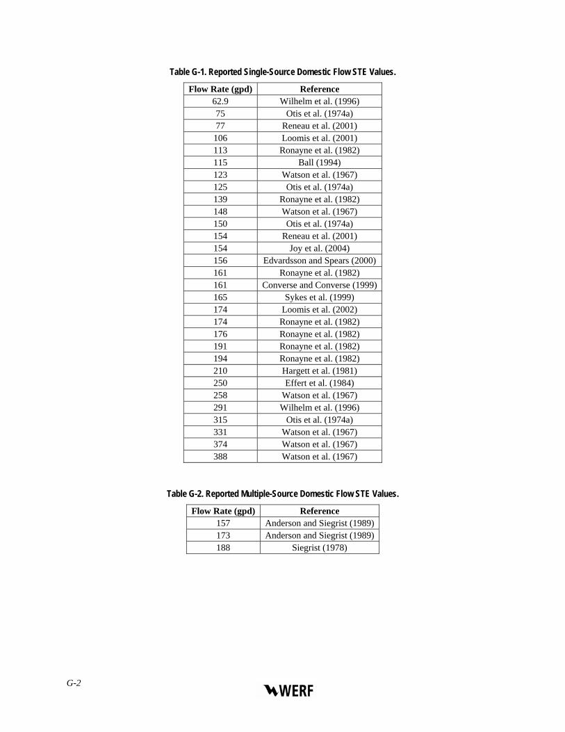
Table G-1. Reported Single-Source Domestic Flow STE Values.
Flow Rate (gpd) Reference 62.9 Wilhelm et al. (1996) 75 Otis et al. (1974a) 77 Reneau et al. (2001)
106 Loomis et al. (2001) 113 Ronayne et al. (1982) 115 Ball (1994) 123 Watson et al. (1967) 125 Otis et al. (1974a) 139 Ronayne et al. (1982) 148 Watson et al. (1967) 150 Otis et al. (1974a) 154 Reneau et al. (2001) 154 Joy et al. (2004) 156 Edvardsson and Spears (2000) 161 Ronayne et al. (1982) 161 Converse and Converse (1999) 165 Sykes et al. (1999) 174 Loomis et al. (2002) 174 Ronayne et al. (1982) 176 Ronayne et al. (1982) 191 Ronayne et al. (1982) 194 Ronayne et al. (1982) 210 Hargett et al. (1981) 250 Effert et al. (1984) 258 Watson et al. (1967) 291 Wilhelm et al. (1996) 315 Otis et al. (1974a) 331 Watson et al. (1967) 374 Watson et al. (1967) 388 Watson et al. (1967)
Table G-2. Reported Multiple-Source Domestic Flow STE Values.
Flow Rate (gpd) Reference 157 Anderson and Siegrist (1989) 173 Anderson and Siegrist (1989) 188 Siegrist (1978)
G-2

Table G-3. Reported Food Source Flow STE Values.
Flow Rate (gpd) Reference 73.2 Bloomquist and Schmidt (1995) 90.5 Bloomquist and Schmidt (1995) 181 Bloomquist and Schmidt (1995) 201 Bloomquist and Schmidt (1995) 230 Bloomquist and Schmidt (1995) 256 Bloomquist and Schmidt (1995) 450 Siegrist et al. (1984b) 528 Siegrist et al. (1984b) 766 Siegrist et al. (1984b) 1558 Siegrist et al. (1984b) 1638 Siegrist et al. (1984b) 3791 Bloomquist and Schmidt (1995)
Table G-4. Reported Non-medical Source Flow STE Values.
Flow Rate (gpd) Source Reference 30 Office Ronayne et al. (1982) 99 Correctional Facility McCarthy et al. (1999)
147 Correctional Facility McCarthy et al. (1999) 155 Correctional Facility McCarthy et al. (1999) 175 Correctional Facility McCarthy et al. (1999) 193 Correctional Facility McCarthy et al. (1999) 212 Correctional Facility McCarthy et al. (1999) 218 Correctional Facility McCarthy et al. (1999) 221 Correctional Facility McCarthy et al. (1999) 223 Correctional Facility McCarthy et al. (1999) 227 Correctional Facility McCarthy et al. (1999) 230 Correctional Facility McCarthy et al. (1999) 232 Correctional Facility McCarthy et al. (1999) 235 Correctional Facility McCarthy et al. (1999) 236 Correctional Facility McCarthy et al. (1999) 250 Correctional Facility McCarthy et al. (1999) 253 Correctional Facility McCarthy et al. (1999) 280 Correctional Facility McCarthy et al. (1999) 436 Convenience Store Ball et al. (1999) 845 Golf Club Siegrist et al. (1984b) 3000 Sawmill Ronayne et al. (1982) 3778 Golf Club Siegrist et al. (1984b) 4014 Campsite Ball et al. (1999) 5300 Rest Area/RV Dump Griffin et al. (2002) 5328 Rest Area/RV Dump Griffin et al. (2004)
14100 Motel Siegrist et al. (1984b)
Influent Constituent Characteristics of the Modern Waste Stream from Single Sources G-3

G-4

APPENDIX H
COMPLETE LISTING OF REPORTED OIL AND GREASE VALUES
Influent Constituent Characteristics of the Modern Waste Stream from Single Sources H-1

Table H-1. Reported Single-Source Domestic Oil and Grease Raw Wastewater Values.
Oil and Grease (mg/L) Reference 16 Lawrence (1973) 21 Lawrence (1973) 33 Watson et al. (1967) 41 Watson et al. (1967) 42 Bounds (2004) 65 Watson et al. (1967) 66 Watson et al. (1967) 81 Bounds (1997) 89 Kreissl (1971) 92 Watson et al. (1967) 95 Watson et al. (1967)
122 Bounds (1997) 129 Bounds (1997)) 134 Watson et al. (1967)
Table H-2. Reported Non-medical Source Oil and Grease Raw Wastewater Walues.
Oil and Grease (mg/L) Source Reference 110 Rest Area Pearson et al. (1987) 189 RV Dump/Rest Area Pearson et al. (1987)
Table H-3. Other Reported Fats/Oil/Grease Raw Wastewater Values.
Oil and Grease (mg/L) Source Reference 123 Non-medical, Restaurant Lesikar et al. (2004) 123 Non-medical, Restaurant Lesikar et al. (2004) 4520 Non-medical, Restaurant Lesikar et al. (2004)
Table H-4. Reported Single Source Domestic Oil and Grease STE Values.
Oil and Grease (mg/L) Reference 31 Rich et al. (2003) 32 Rich et al. (2003) 35 Rich (2006) 36 Sherman and Anderson (1991)
H-2

Table H-5. Reported Food Source Oil and Grease STE Values.
Oil and Grease (mg/L) Reference 9 Bloomquist and Schmidt (1995)
10 Bloomquist and Schmidt (1995) 10.2 Bloomquist and Schmidt (1995) 12.1 Bloomquist and Schmidt (1995) 13.6 Bloomquist and Schmidt (1995) 20.6 Bloomquist and Schmidt (1995) 21 Bloomquist and Schmidt (1995)
23.6 Bloomquist and Schmidt (1995) 23.7 Bloomquist and Schmidt (1995) 25.8 Bloomquist and Schmidt (1995) 30.3 Bloomquist and Schmidt (1995) 31.4 Bloomquist and Schmidt (1995) 34 Bloomquist and Schmidt (1995) 35 Bloomquist and Schmidt (1995) 40 Siegrist et al. (1984b) 40 Bloomquist and Schmidt (1995)
40.8 Bloomquist and Schmidt (1995) 47 Siegrist et al. (1984b) 49 Siegrist et al. (1984b) 50 Bloomquist and Schmidt (1995) 50 Bloomquist and Schmidt (1995)
52.6 Bloomquist and Schmidt (1995) 65 Siegrist et al. (1984b)
79.4 Bloomquist and Schmidt (1995) 91 Bloomquist and Schmidt (1995)
92.4 Bloomquist and Schmidt (1995) 101 Siegrist et al. (1984b) 101 Siegrist et al. (1984b) 101 Bloomquist and Schmidt (1995) 115 Bloomquist and Schmidt (1995) 122 Bloomquist and Schmidt (1995) 125 Bloomquist and Schmidt (1995) 142 Bloomquist and Schmidt (1995) 144 Siegrist et al. (1984b) 160 Bloomquist and Schmidt (1995) 300 Bloomquist and Schmidt (1995) <5 Bloomquist and Schmidt (1995) <5 Bloomquist and Schmidt (1995)
Influent Constituent Characteristics of the Modern Waste Stream from Single Sources H-3

Table H-6. Reported Non-medical Source Oil and Grease STE Values.
Oil and Grease (mg/L) Source Reference 6 Marina Matassa et al. (2003) 8 Marina Matassa et al. (2003) 8 Campground Matassa et al. (2003) 9 Marina Matassa et al. (2003)
24 Golf club Siegrist et al. (1984b) 24 Campground Matassa et al. (2003) 33 Golf club Siegrist et al. (1984b) 40 Marina Matassa et al. (2003) 45 Motel Siegrist et al. (1984b) 46 Golf club Siegrist et al. (1984b) 49 Marina Matassa et al. (2003) 91 Marina Matassa et al. (2003) 98 Marina Matassa et al. (2003)
130 Marina Matassa et al. (2003) 140 Campground Matassa et al. (2003)
H-4

APPENDIX I
COMPLETE LISTING OF OTHER REPORTED VALUES
Influent Constituent Characteristics of the Modern Waste Stream from Single Sources I-1

Table I-1. Reported pH Values.
Average Value Source Waste Stream Reference 6 Raw Single-source domestic Dietzman and Gross (2003)
6.08 Raw Single-source domestic Dietzman and Gross (2003) 6.12 Raw Single-source domestic Dietzman and Gross (2003) 6.18 Raw Single-source domestic Dietzman and Gross (2003) 6.36 Raw Single-source domestic Dietzman and Gross (2003) 6.9 Raw Single-source domestic Bounds (2004)
7.11 Raw Single-source domestic Hanson et al. (2002) 7.2 Raw Single-source domestic Lawrence (1973)
7.35 Raw Single-source domestic Hanson et al. (2002) 7.4 Raw Single-source domestic Bennett et al. (1974) 7.5 Raw Single-source domestic Edvardsson and Spears (2000) 7.5 Raw Single-source domestic Lawrence (1973) 7.6 Raw Single-source domestic Thiruvenkatachari (1976) 7.6 Raw Single-source domestic Watson et al. (1967) 7.8 Raw Single-source domestic Bounds (1997) 8 Raw Single-source domestic Watson et al. (1967) 8 Raw Single-source domestic Watson et al. (1967)
8.2 Raw Single-source domestic Watson et al. (1967) 8.3 Raw Single-source domestic Watson et al. (1967)
8.37 Raw Single-source domestic Hanson et al. (2002) 8.4 Raw Single-source domestic Watson et al. (1967) 7.4 Raw Non-medical, RV Dump Pearson et al. (1987) 7.8 Raw Non-medical, Rest Area Restroom Pearson et al. (1987) 6.4 STE Single-source domestic Robertson and Blowes (1995) 6.5 STE Single-source domestic Seabloom et al. (1981) 6.7 STE Single-source domestic Wilhelm et al. (1996) 6.9 STE Single-source domestic Thom et al. (1998) 6.9 STE Single-source domestic Viraraghavan and Warnock (1974) 6.9 STE Single-source domestic Seabloom et al. (1981) 6.9 STE Single-source domestic Thiruvenkatachari (1976) 7 STE Single-source domestic Thom et al. (1998) 7 STE Single-source domestic Seabloom et al. (1981) 7 STE Single-source domestic Seabloom et al. (1981)
7.0 STE Single-source domestic Hanson et al. (2002) 7.1 STE Single-source domestic Reneau et al. (2001) 7.1 STE Single-source domestic Hampton and Jones (1984) 7.1 STE Single-source domestic Seabloom et al. (1981) 7.1 STE Single-source domestic Engeset and Seabloom (1978) 7.2 STE Single-source domestic Siegrist and Boyle (1987) 7.2 STE Single-source domestic Wilhelm et al. (1996) 7.2 STE Single-source domestic Reneau et al. (2001) 7.3 STE Single-source domestic Thom et al. (1998) 7.4 STE Single-source domestic Converse and Converse (1998)
7.46 STE Single-source domestic Huang et al. (1994) 7.48 STE Single-source domestic Patterson (2004) 7.5 STE Single-source domestic Ball (1994)
7.52 STE Single-source domestic Hampton and Jones (1984)
I-2

Table I-1. Reported pH Values (continued).
Average Value Source Waste Stream Reference 7.6 STE Single-source domestic Converse et al. (1994) 7.7 STE Single-source domestic Penninger and Hoover (1998) 8 STE Single-source domestic Penninger and Hoover (1998)
7.36 STE Multiple-source domestic Brown et al. (1977) 7.55 STE Multiple-source domestic Neralla et al. (1998) 7.69 STE Multiple-source domestic Neralla et al. (1998) 8.4 STE Multiple-source domestic Converse et al. (1991) 6.1 STE Non-medical, Dairy Farm Christopherson et al. (2004) 6.2 STE Non-medical, Dairy Farm Christopherson et al. (2004) 6.2 STE Non-medical, Dairy Farm Christopherson et al. (2004)
6.25 STE Non-medical, Marina Matassa et al. (2003) 6.7 STE Non-medical, Dairy Farm Christopherson et al. (2004)
6.84 STE Non-medical, Marina Matassa et al. (2003) 6.89 STE Non-medical, Marina Matassa et al. (2003) 6.96 STE Non-medical, Campground Matassa et al. (2003) 6.99 STE Non-medical, Marina Matassa et al. (2003)
7 STE Non-medical, Dairy Farm Christopherson et al. (2004)
7 STE Non-medical, Correctional Institute Boyle et al. (1994)
7 STE Non-medical, Marina Matassa et al. (2003) 7 STE Non-medical, Marina Matassa et al. (2003)
7.08 STE Non-medical, Campground Matassa et al. (2003) 7.09 STE Non-medical, Campground Matassa et al. (2003) 7.1 STE Single source domestic Kristiansen (1981)
7.14 STE Non-medical, Marina Matassa et al. (2003) 7.17 STE Non-medical, Campground Matassa et al. (2003) 7.2 STE Non-medical, Marina Matassa et al. (2003) 7.6 STE Non-medical, Elementary School Harmon et al. (1996)
7.7 STE Non-medical, One room schoolhouse turned into museum Hatch et al. (2002)
8.32 STE Non-medical, Ski Area Baker (1980)
Table I-2. Reported Alkalinity (as CaCO3) Values.
Average Value Source Waste Stream Reference 316.4 STE Single-source domestic Wilhelm et al. (1996) 356 STE Single-source domestic Robertson and Blowes (1995) 374 STE Single-source domestic Wilhelm et al. (1996) 433 STE Single-source domestic Converse and Converse (1998) 479 STE Single-source domestic Siegrist and Boyle (1987) 528 STE Single-source domestic Siegrist et al. (2000) 676 STE Single-source domestic Siegrist et al. (2000) 946 STE Single-source domestic Patterson (2004) 107 STE Non-medical, Elementary School Harmon et al. (1996)
221 STE Non-medical, Correctional Institute Boyle et al. (1994)
361 STE Non-medical, Marina Matassa et al. (2003)
Table I-3. Reported Hardness (as CaCO3) Values.
Average Value Source Waste Stream Reference 327 STE Single-source domestic Siegrist and Boyle (1987)
Influent Constituent Characteristics of the Modern Waste Stream from Single Sources I-3

Table I-4. Reported Temperature (oC) Values.
Average Value Source Waste Stream Reference 17.2 Raw Single-source domestic Hanson et al. (2002) 20.8 Raw Single-source domestic Hanson et al. (2002) 21.2 Raw Single-source domestic Hanson et al. (2002) 36 Raw Single-source domestic Bennett et al. (1974)
10.8 STE Single-source domestic Converse and Converse (1998) 11.3 STE Single-source domestic Thom et al. (1998) 11.8 STE Single-source domestic Seabloom et al. (1981) 11.9 STE Single-source domestic Seabloom et al. (1981) 13 STE Single-source domestic Seabloom et al. (1981)
13.3 STE Single-source domestic Seabloom et al. (1981) 14.3 STE Single-source domestic Seabloom et al. (1981) 14.7 STE Single-source domestic Thom et al. (1998) 15.1 STE Single-source domestic Rich (2006) 15.4 STE Single-source domestic Hanson et al. (2002) 17.8 STE Single-source domestic Thom et al. (1998) 7.2 STE Multiple-source domestic Siegrist et al. (1991)
15.5 STE Non-medical, Office/Manufacturing Weaver et al. (1998)
16 STE Non-medical, Correctional Institute Boyle et al. (1994)
19.4 STE Non-medical, Office/Manufacturing Weaver et al. (1998)
Table I-5. Reported Dissolved Oxygen (mg/L) Values.
Average Value Source Waste Stream Reference 0.825 Raw Single-source domestic Hanson et al. (2002) 0.922 Raw Single-source domestic Hanson et al. (2002) 1.63 Raw Single-source domestic Hanson et al. (2002)
0 STE Single-source domestic Seabloom et al. (1981) 0.4 STE Single-source domestic Seabloom et al. (1981) 0.5 STE Single-source domestic Thom et al. (1998)
0.51 STE Single-source domestic Thom et al. (1998) 0.8 STE Single-source domestic Ball (1994)
0.992 STE Single-source domestic Hanson et al. (2002) 1 STE Single-source domestic Thom et al. (1998)
1.3 STE Single-source domestic Seabloom et al. (1981) 1.3 STE Single-source domestic Engeset and Seabloom (1978) 1.6 STE Single-source domestic Seabloom et al. (1981) 1.8 STE Single-source domestic Seabloom et al. (1981)
0.8 STE Non-medical, Office/Manufacturing Weaver et al. (1998)
1.5 STE Non-medical, Office/Manufacturing Weaver et al. (1998)
II-4

Table I-6. Reported Turbidity (ntu) Values.
Average Value Source Waste Stream Reference 80 Raw Single-source domestic Edvardsson and Spears (2000) 45 STE Single-source domestic Siegrist and Boyle (1987) 57 STE Multiple-source domestic Neralla et al. (1998)
117 STE Non-medical, Office/Manufacturing Weaver et al. (1998)
155 STE Non-medical, Office/Manufacturing Weaver et al. (1998)
Table I-7. Reported Anion and Cation (mg/L) Values.
Average Value Constituent Source Waste Stream Reference
0.1 Aluminum STE Non-medical, Campground Ptacek (1998) 9 Calcium STE Single-source domestic Robertson and Blowes (1995)
14.3 Calcium STE Single-source domestic Wilhelm et al. (1996) 41.2 Calcium STE Single-source domestic Wilhelm et al. (1996) 59 Calcium STE Single-source domestic Siegrist and Boyle (1987)
83.6 Calcium STE Non-medical, Campground Ptacek (1998) 137 Calcium STE Non-medical, Elementary School Harmon et al. (1996)
83.17 Chloride Raw Single-source domestic Hanson et al. (2002) 716.3 Chloride Raw Single-source domestic Hanson et al. (2002)
1096.2 Chloride Raw Single-source domestic Hanson et al. (2002) 35.5 Chloride STE Single-source domestic Reneau et al. (2001) 37.25 Chloride STE Single-source domestic Hanson et al. (2002) 38.5 Chloride STE Single-source domestic Thom et al. (1998) 40 Chloride STE Single-source domestic Wilhelm et al. (1996)
40.4 Chloride STE Single-source domestic Reneau et al. (2001) 48.4 Chloride STE Single-source domestic Wolf et al. (1998) 50.9 Chloride STE Single-source domestic Lindbo and MacConnell (2001) 53 Chloride STE Single-source domestic Viraraghavan and Warnock (1974) 53 Chloride STE Single-source domestic Robertson and Blowes (1995)
54.8 Chloride STE Single-source domestic Wilhelm et al. (1996) 58.6 Chloride STE Single-source domestic Huang et al. (1994) 62 Chloride STE Single-source domestic Thom et al. (1998)
62.2 Chloride STE Single-source domestic Thom et al. (1998) 63.2 Chloride STE Single-source domestic Seabloom et al. (1981) 69 Chloride STE Single-source domestic Converse (1999) 70 Chloride STE Single-source domestic Walker et al. (1973) 70 Chloride STE Single-source domestic Walker et al. (1973)
70.1 Chloride STE Single-source domestic Lindbo and MacConnell (2001) 113 Chloride STE Single-source domestic Seabloom et al. (1981) 130 Chloride STE Single-source domestic Walker et al. (1973) 146 Chloride STE Single-source domestic Seabloom et al. (1981) 147 Chloride STE Single-source domestic Penninger and Hoover (1998) 150 Chloride STE Single-source domestic Walker et al. (1973) 189 Chloride STE Single-source domestic Seabloom et al. (1981) 270 Chloride STE Single-source domestic Seabloom et al. (1981) 378 Chloride STE Single-source domestic Converse and Converse (1998) 417 Chloride STE Single-source domestic Converse et al. (1994) 97 Chloride STE Multiple-source domestic Cogger et al. (1988)
Influent Constituent Characteristics of the Modern Waste Stream from Single Sources I-5

Table I-7. Reported Anion and Cation (mg/L) Values (continued).
Average Value Constituent Source Waste Stream Reference
183 Chloride STE Multiple-source domestic Brown et al. (1977) 275 Chloride STE Multiple-source domestic Converse et al. (1991) 57 Chloride STE Non-medical, Campground Ptacek (1998)
60 Chloride STE Non-medical, Correctional Institution Boyle et al. (1994)
70 Chloride STE Non-medical, Campus Christian Center & Dorm Anderson et al. (1994)
0.029 Chloride STE Non-medical, Campground Ptacek (1998) 0.067 Iron STE Single-source domestic Wilhelm et al. (1996) 0.248 Iron STE Single-source domestic Wilhelm et al. (1996) 0.599 Iron STE Non-medical, Campground Ptacek (1998) 3.4 Magnesium STE Single-source domestic Wilhelm et al. (1996) 14 Magnesium STE Single-source domestic Wilhelm et al. (1996) 33 Magnesium STE Single-source domestic Siegrist and Boyle (1987)
12.9 Magnesium STE Non-medical, Campground Ptacek (1998) 25 Magnesium STE Non-medical, Elementary School Harmon et al. (1996)
0.48 Manganese STE Non-medical, Campground Ptacek (1998) 11.7 Potassium STE Single-source domestic Wilhelm et al. (1996) 21.8 Potassium STE Single-source domestic Wilhelm et al. (1996) 27 Potassium STE Single-source domestic Robertson and Blowes (1995) 18 Potassium STE Multiple-source domestic Cogger et al. (1988)
20.6 Potassium STE Non-medical, Campground Ptacek (1998) 43 Potassium STE Non-medical, Elementary School Harmon et al. (1996)
19.42 Sulfate Raw Single-source domestic Hanson et al. (2002) 39.36 Sulfate Raw Single-source domestic Hanson et al. (2002) 216.1 Sulfate Raw Single-source domestic Hanson et al. (2002) 5.68 Sulfate STE Single-source domestic Duncan et al. (1994)
9 Sulfate STE Single-source domestic Robertson and Blowes (1995) 11.9 Sulfate STE Single-source domestic Thom et al. (1998) 16.6 Sulfate STE Single-source domestic Thom et al. (1998) 17.08 Sulfate STE Single-source domestic Otis et al. (1974b) 18.8 Sulfate STE Single-source domestic Thom et al. (1998) 34.1 Sulfate STE Non-medical, Campground Ptacek (1998) 6.9 Sulfate1 STE Single-source domestic Wilhelm et al. (1996)
11.8 Sulfate1 STE Single-source domestic Wilhelm et al. (1996) 59 Sulfate1 STE Non-medical, Elementary School Harmon et al. (1996) 3.5 Sulfide STE Single-source domestic Seabloom et al. (1981) 5.5 Sulfide STE Single-source domestic Seabloom et al. (1981)
10.7 Sulfide STE Single-source domestic Seabloom et al. (1981) 39 Sodium STE Singlesource domestic Robertson and Blowes (1995)
84.9 Sodium STE Single-source domestic Wilhelm et al. (1996) 89.7 Sodium STE Single-source domestic Wilhelm et al. (1996) 218 Sodium STE Single-source domestic Siegrist and Boyle (1987) 174 Sodium STE Multiple-source domestic Cogger et al. (1988) 42.8 Sodium STE Non-medical, Campground Ptacek (1998) 107 Sodium STE Non-medical, Elementary School Harmon et al. (1996) 0.6 Zinc Raw Non-medical, Rest Area Restroom Pearson et al. (1987) 9 Zinc Raw Non-medical, RV Dump Pearson et al. (1987)
0.069 Zinc STE Non-medical, Campground Ptacek (1998) 1 Sulfate as mg-S/L
I-6

Influent Constituent Characteristics of the Modern Waste Stream from Single Sources
REFERENCES R.1 Report References Albert, J.M., J. Munakata-Marr, L. Tenorio, and R.L. Siegrist (2003). Statistical evaluation of bacterial source tracking data obtained by rep-PCR DNA fingerprinting of Escherichia coli. Environmental Science and Technology, 37(20): 4554-4560. American Housing Survey (AHS) (2006). http://www.census.gov/hhes/www/housing/ahs/ahs.html Anderson, D.L. and R.L. Siegrist (1989). The performance of ultra-low-volume flush toilets in Phoenix. Journal of the American Water Works Association, 81(3): 52-57. Anderson, D.L. and A.L. Lewis (1992). Human enterovirus monitoring at onsite wastewater disposal systems. Proceedings of the Seventh Northwest On-Site Wastewater Treatment Short Course and Equipment Exhibition, University of Washington. Anderson, D.L., A.L. Lewis, and K.M. Sherman (1992). Human enterovirus monitoring at onsite sewage disposal systems in Florida. Proceedings of the Sixth National Symposium on Individual and Small Community Sewage Systems, ASAE, St. Joseph, MI. Anderson, D.L., D. Mulville-Friel, and W.L. Nero (1993). The impact of water conserving plumbing fixtures on residential water use in Tampa, FL. Proceedings of ConServ 93, American Water Works Association, 611-628. Ansari, S.A., S.R. Farrah, and G.R. Chaudhry (1992). Presence of human immunodeficiency virus nucleic acids in wastewater and their detection by polymerase chain reaction. Applied and Environmental Microbiology, 58(12): 3984-3990. American Public Health Association (APHA) (2005). Standard Methods for the Examination of Water and Wastewater. Washington, D.C., American Public Health Association. Atlas, R.M. and R. Bartha (1998). Microbial Ecology: Fundamentals and Applications. Menlo Park, CA, Benjamin/Cummings Science Publishing. Ball, H., M. Reinhard, and P.L. McCarty (1989). Biotransformation of halogenated and nonhalogenated octyphenol polyethoxylate residues under aerobic and anaerobic conditions. Environmental Science and Technology, 23(8):951-961. Barber, L., G. Brown, and S. Zaugg (2000). Potential endocrine disrupting organic chemicals in treated municipal wastewater and river water, upper Midwest, USA. Analysis of Environmental Endocrine Disruptors. American Chemical Society Symposium Series No. 747. American Chemical Society, Washington, D.C.
R-1

Bechdol, M.L., A.J. Gold, and J.H. Gorres (1995). Modeling viral contamination from on-site wastewater disposal in coastal watersheds. Proceedings of the Seventh National Symposium on Individual and Small Community Sewage Systems, ASAE, St. Joseph, MI. Belfroid, A.C., A. Van der Horst, A.D. Vethaak, A.J. Schfer, G.B.J. Jijs, J. Wegener, and W.P. Cofins (1999). Analysis and occurrence of estrogenic hormones and their glucuronides in surface water and wastewater in the Netherlands. Science of the Total Environment, 225:101-108. Bitton, G. (1999). Wastewater Microbiology. New York, Wiley-Liss, Inc. Brown and Caldwell (1984). Residential water conservation projects. Research Report 903. Washington, D.C., U.S. Department of Housing and Urban Development, Office of Policy Development. Brown, K.W., J.F. Slowey, and H.W. Wolf (1980). The movement of salts, nutrients, fecal coliform and virus below septic leach fields in three soils. Proceedings of the Second National Symposium on Individual and Small Community Sewage Systems, ASAE, St. Joseph, MI. Cahill, J.D., E.T. Furlong, M.R. Burkhardt, D.W. Kolpin, and L.G. Anderson (2004). Determination of pharmaceutical compounds in surface- and ground-water samples by solid-phase extraction and high-performance liquid chromatography-electrospray ionization mass spectrometry. Journal of Chromatography, 1041:171-180. Cole, C.A. and W.E. Sharpe (1983). Impact of water conservation on residential septic tank effluent quality. Proceedings of the Third National Symposium on Individual and Small Community Sewage Systems, ASAE, St. Joseph, MI. Converse, J.C., M.E. Kean, E.J. Tyler, and J.O. Peterson (1992). Bacterial and nutrient removal in Wisconsin at-grade on-site systems. Proceedings of the Sixth National Symposium on Individual and Small Community Sewage Systems, ASAE, St. Joseph, MI. Crites, R. and G. Tchobanoglous (1998). Small and Decentralized Wastewater Management Systems. McGraw-Hill, San Francisco, CA. Dean, R.B. and E. Lund (1981). Water Reuse: Problems and Solutions. London, Academic Press. DeJong, K.E., R.L. Siegrist, L.B. Barber, and A.L. Wren (2004). Occurrence of emerging organic chemicals in wastewater effluents from onsite systems. On-site Wastewater Treatment: Proceedings of the Tenth National Symposium on Individual and Small Community Sewage Systems, Amer. Soc. Agric. Engineers, 400-407. DeJong, K.E., L.B. Barber, G.K. Brown, and R.L. Siegrist (2006). Occurrence and fate of organic wastewater contaminants during onsite wastewater treatment. In press, Environmental Science and Technology.
R-2

Influent Constituent Characteristics of the Modern Waste Stream from Single Sources
Deng, M.Y. and D.O. Cliver (1995a). Mixed waste studies with viruses and Giardia. Proceedings of the Seventh National Symposium on Individual and Small Community Sewage Systems, ASAE, St. Joseph, MI. Deng, M.Y. and D.O. Cliver (1995b). Persistence of inoculated Hepatitis A virus in mixed human and animal wastes. Applied and Environmental Microbiology, 61(1): 87-91. Desbrow, C., E.J. Routledge, G.C. Brighty, J.P. Sumpter, and M. Waldock (1998). Identification of estrogenic chemicals in STW effluent. 1. Chemical fractionation and in vitro biological Screening. Environmental Science and Technology, 32(11): 1549-1558. DeWalle, F.B., D.A. Kalman, D. Norman, J. Sung, and G. Plews (1980). Trace organic removals in a large septic tank. In R.W. Seabloom (ed.), Proceedings of the Fourth Northwest Onsite Wastewater Disposal Short Course, University of Washington, Seattle, WA, p. 212-236. Eriksson, E., K. Auffarth, A-M. Eilersen, M. Henze, and A. Ledin (2003). Household chemicals and personal care products as sources for xenobiotic organic compounds in grey wastewater. Water SA, 29: 135-146. Gerba, C.P. (1989). Virus survival and transport in groundwater. Proceedings of the Sixth Northwest On-Site Wastewater Treatment Short Course and Equipment Exhibition, University of Washington. Gerba, C.P. (2002). Virus transport and fate in groundwater. Proceedings of the Eleventh Northwest On-Site Wastewater Treatment Short Course and Equipment Exhibition, University of Washington. Gerba, C.P. and G. Bitton (1984). Microbial pollutants: Their survival and transport pattern in groundwater. Groundwater Pollution Microbiology. New York, John Wiley & Sons. Giger, W., P.H. Brunner, and C. Schaffner (1984). 4-Nonylphenol in sewage sludge: accumulation of toxic metabolites from nonionic surfactants. Science, 225: 623-625. Gilbert, R.G., C.P. Gerba, R.C. Rice, H. Bouwer, C. Wallis, and J.L. Melnick (1976). Virus and bacteria removal from wastewater by land treatment. Applied and Environmental Microbiology, 32(3): 333-338. Glassmeyer, S.T., E.T. Furlong, D.W. Kolpin, J.D. Cahill, S.D. Zaugg, S.L. Werner, M.T. Meyer, and D.D. Kryak (2005). Transport of chemical and microbial compounds from known wastewater discharges: potential for use as indicators of human fecal contamination. Environmental Science and Technology, 39: 5157-5169. Godfrey, E. (2004). Screening level study of pharmaceuticals in septic tank, ground water, and surface water in Missoula, Montana. Master’s Thesis, University of Montana, Missoula, MT. Goyal, S.M., K.S. Zerda, and C.P. Gerba (1980). Concentrations of coliphages from large volumes of water and wastewater. Applied and Environmental Microbiology, 39(1): 85-91.
R-3

Green, K.M. and D.O. Cliver (1977). Removal of virus from septic tank effluent by sand columns. Proceedings of the First National Symposium on Individual and Small Community Sewage Systems. Greer, B.A. and W.C. Boyle (1987). Volatile organic compounds (VOCs) in small community wastewater disposal systems using soil absorption. In Proceedings of the Fifth National Symposium on Individual and Small Community Sewage Treatment, American Society of Agricultural Engineers, St. Joseph, MI., p. 284-293. Hagedorn, C. (1984). Microbiological aspects of groundwater pollution due to septic tanks. Groundwater Pollution Microbiology. New York, John Wiley & Sons: 181-195. Hass, C.N., J.B. Rose, and C.P. Gerba (1999). Quantitative Microbial Risk Assessment. New York, John Wiley & Sons, Inc. Hinkle, S.R., R.J. Weick, J.M. Johnson, J.D. Cahill, S.G. Smith, and B.J. Rich (2005). Organic wastewater compounds, pharmaceuticals, and coliphage in ground water receiving discharge from onsite wastewater treatment systems near La Pine, Oregon: Occurrence and implications for transport. U.S. Geological Survey Scientific Investigations Report 2005-5055, 98 p. Kanter, R.D., E.J. Tyler, and J.C. Converse (1998). A denitrification system for domestic wastewater using sulfur oxidizing bacteria. Proceedings of the Eight National Symposium on Individual and Small Community Sewage Systems, ASAE, St. Joseph, MI. Jobling, S., D. Sheahan, J.A. Osborne, P. Matthiessen, and J.P. Sumpter (1996). Inhibition of testicular growth in rainbow trout (Oncorhynchus mykiss) exposed to estrogenic alkylphenolic chemicals. Environmental Toxicology and Chemistry, 15: 194-202. Keswick, B.H., D. Wang, and C.P. Gerba (1982). The use of microorganisms as groundwater tracers: A review. Ground Water, 20(2): 142-149. Kolpin, D.W., E.T. Furlong, M.T. Meyer, E.M. Thurman, S.D. Zaugg, L.B. Barber, and H.T. Buxton (2002). Pharmaceuticals, hormones, and other organic wastewater contaminants in U.S. Streams, 1999-2000: A National Reconnaissance. Environmental Science and Technology, 36: 1202-1211. Kirkland, S.L. (2001). Coupling site-scale fate and transport with watershed-scale modeling to assess the cumulative effects of nutrients from decentralized onsite wastewater systems. Master’s Thesis, Colorado School of Mines, Golden, Colorado. Lago, P.M., H.E. Gary Jr., L.S. Perez, V. Caceres, J.B. Olivera, R.P. Puentes, M.B. Corredor, P. Jimenez, M.A. Pallansch, and R.G. Cruz (2003). Poliovirus detection in wastewater and stools following an immunization campaign in Havana, Cuba. International Journal of Epidemiology, 32: 772-777.
R-4

Influent Constituent Characteristics of the Modern Waste Stream from Single Sources
Lisle, J.T., J.J. Smith, D.D. Edwards, and G.A. McFeters (2004). Occurrence of microbial indicators and Clostridium perfringens in wastewater, water column samples, sediments, drinking water, and weddel seal feces collected at McMurdo Station, Antarctica. Applied and Environmental Microbiology, 70(12): 7269-7276. Logan, A.J., T.K. Stevik, R.L. Siegrist, and R.M. Ronn (2001). Transport and fate of Cryptosporidium parvum in intermittent sand filters during wastewater treatment. Proceedings of the Ninth National Symposium on Individual and Small Community Sewage Systems, ASAE, St. Joseph, MI. Madigan, M.T., J.M. Martinko, and J. Parker (1997). Brock Biology of Microorganisms. Upper Saddle River, New Jersey, Simon & Schuster. Mayer, P.W., W.B. DeOreo, E.M. Optiz, J.C. Kiefer, W.Y. Davis, B. Dziegielewski, and J.O. Nelson (1999). Residential End Uses of Water, American Water Works Association Research Foundation, Denver, Colorado, 310 p. McAvoy, D.C., C.E. White, B.L. Moore, and R.A. Rapaport (1994). Chemical fate and transport in a domestic septic system: sorption and transport of anionic and cationic surfactants. Environmental Toxicology and Chemistry, 13: 213-221. McCoy, E. and W.A. Ziebell (1975). The effects of effluents on groundwater: Bacteriological aspects. Proceedings of the Second Individual Onsite Wastewater Systems, Ann Arbor Science. McGinnis, J.A. and F.B. DeWalle (1982). Typhoid organism travel in saturated permeable soil in Yakima, Washington. Proceedings of the Fourth Northwest On-Site Wastewater Treatment Short Course and Equipment Exhibition, University of Washington. Mehnert, D.U. and K.E. Stewein (1993). Detection and distribution of rotavirus in raw sewage and creeks in Sao Paulo, Brazil. Applied and Environmental Microbiology, 59(1): 140-143. Metcalf and Eddy, Inc. (1991). Wastewater Engineering: Treatment, Disposal and Reuse. 3rd Ed. McGraw-Hill, New York. Meyer, M.T., J.E. Bumgarner, J.L. Varns, J.V. Daughtridge, E.M. Thurman, and K.A. Hostetler (2001). Use of a radioimmunoassay as a screen for antibiotics in confined animal feeding operations and confirmation by liquid chromatography/mass spectrometry. Science of the Total Environment, 248:181-187. National Climatic Data Center (U.S. Department of Commerce) (2006). http://www.ncdc.noaa.gov/oa/ncdc.html New Mexico Environment Department (2006). http://www.nmenv.state.nm.us/fod/LiquidWaste/index.html Nicosia, L.A., J.B. Rose, L. Stark, and M.T. Stewart (2001). A field study of virus removal in septic tank drainfields. Journal of Environmental Quality, 30: 1933-1939.
R-5

Nielson, A.M., A.J. DeCarvalho, D.C. McAvoy, L. Kravetz, M.L. Cano, and D.L. Anderson (2002). Investigation of an onsite wastewater treatment system in sandy soil: Site characterization and fate of anionic and nonionic surfactants. Environmental Toxicology and Chemistry, 21: 2606-2616. North Carolina-Department of Environmental and Natural Resources- On-site Wastewater Section http://www.deh.enr.state.nc.us/osww_new//largewwsys.htm Robertson, W.D. (1994). Chemical fate and transport in a domestic septic system: Site description and attenuation of dichlorobenzene. Environmental Toxicology and Chemistry, 13: 183-191. Rose, J.B., D.W. Griffin, and L.W. Nicosia (1999). Virus transport from septic tanks to coastal waters. Proceedings of the Tenth Northwest On-Site Wastewater Treatment Short Course and Equipment Exhibition, University of Washington. Sakai, K. (1999). Studies on endocrine disrupting chemicals in sewage treatment plants. Gesuido Kyokaishi, 36(445): 34-38. Schweizer, H. (2001). Triclosan: A widely used biocide and its link to antibiotics. FEMS Microbiology Letters, 202: 1-7. Sedmak, G., D. Bina, J. MacDonald, and L. Couillard (2005). Nine-year study of the occurrence of culturable viruses in source water for two drinking water treatment plants and the influent and effluent of a wastewater treatment plant in Milwaukee, Wisconsin (August 1994 through July 2003). Applied and Environmental Microbiology, 71(2): 1042-1050. Sekela, M., R. Brewer, G. Moyle, and T. Tuominen (1999). Occurrence of an environmental estrogen (4-nonylphenol) in sewage treatment plant effluent and the aquatic receiving environment. Water Science and Technology, 39(10-11): 217-220. Shimp, R.J., E.V. Lapsins, and R.M. Ventullo (1994). Chemical fate and transport in a domestic septic system: biodegradation of linear alkylbenzene sulfonate (LAS) and nitrilotriacetic acid (NTA). Environmental Toxicology and Chemistry, 13:2 05-212. Siegrist, R.L. (1978). Characterization of rural household wastewater, Master’s Thesis, University of Wisconsin-Madison, Madison, WI, 150 p. Siegrist, R.L. and W.C Boyle (1987). Wastewater-induced soil clogging development, Journal of Environmental Engineering, 113(3): 550-556. Siegrist, R.L. (2001). Perspectives on the science and engineering of onsite wastewater systems. Small Flows, 2(4): 8-13. Snowdon, J.A., D.O. Clover, and J.C. Converse (1989). Human and animal wastes mixed for disposal to land: Inactivation of viruses and parasites in a laboratory model. Proceedings of the Fifth National Symposium on Individual and Small Community Sewage Systems, ASAE, St. Joseph, MI.
R-6

Influent Constituent Characteristics of the Modern Waste Stream from Single Sources
Stewart, L.W. and J.R.B. Reneau (1983). Movement of fecal coliform bacteria from septic tank effluent through coastal plain soils with high seasonal fluctuating water tables. Proceedings of the Third National Symposium on Individual and Small Community Sewage Systems, ASAE, St. Joseph, MI. Sumpter, J. and S. Jobling (1995). Vitellogenesis as a biomarker for estrogenic contamination of the aquatic environment. Environmental Health Perspectives, 103: 173-178. Ternes, T.A., M. Stumpf, J. Mueller, K. Haberer, R.-D. Wilken, and M. Servos (1999). Behavior and occurrence of estrogens in municipal sewage treatment plants- I. Investigations in Germany, Canada and Brazil. Science of the Total Environment, 225: 81-90. Ternes, T.A., P.M. Kreckel, and J. Mueller (1999). Behavior and occurrence of estrogens in municipal sewage treatment plants- II. Aerobic batch experiments with activated sludge. Science of the Total Environment, 225: 91-99. Thomann, R.V. and J.A. Mueller (1987). Principles of Surface Water Quality Modeling and Control. Harper Collins Publishers Inc. New York, NY. U.S. Census Bureau (2004). American Housing Survey for the United States: 2003. Current Housing Reports, Series H150/03. U.S. Government Printing Office, Washington, D.C. U.S. Census Bureau (2006). http://www.census.gov/ U.S. EPA (1997). Response to Congress on Use of Decentralized Wastewater Treatment Systems. U.S. Environmental Protection Agency, Office of Water, Washington, D.C. U.S. EPA (2002). Onsite Wastewater Treatment Systems Manual. Report No. 625/R-00/008. U.S. Environmental Protection Agency, Cincinnati, OH. Vajda, A.M., L.B. Barber, J. Gray, E.M. Lopez, J.D. Woodling, and D.O. Norris (2005). Intersex and other forms of reproductive disruption in whit suckers (Catostomus commersoni) downstream of a Colorado wastewater treatment plant effluent. Poster display at the South Platte Forum / Emerging Contaminants Workshop. Longmont, CO: Consortium for Research and Education on Emerging Contaminants (CREEC). Van Cuyk, S. (2003). Fate of virus during wastewater renovation in soil porous media biofilters. Environmental Science and Engineering. Golden, Colorado, Colorado School of Mines. Van Cuyk, S., R.L. Siegrist, K.S. Lowe, and R.W. Harvey (2004). Vadose zone processes and chemical transport: Evaluating microbial purification during soil treatment of wastewater with multicomponent tracer and surrogate tests. Journal of Environmental Quality, 33: 316-329. Vanderford, B.J., R.A. Pearson, D.J. Rexing, and S.A. Snyder (2003). Analysis of endocrine disruptors, pharmaceuticals, and personal care products in water using liquid chromatography/tandem mass spectroscopy. Analytical Chemistry, 75: 6265-6274.
R-7

Viraraghavan, T. and S. Hashem (1986). Trace organics in septic tank effluent. Water, Air, and Soil Pollution, 28: 299-308. Ward, R.L., C.S. Ashley, and R.H. Moseley (1976). Heat inactivation of poliovirus in wastewater sludge. Applied and Environmental Microbiology, 32(3): 339-346. Yates, M.V. and S.R. Yates (1997). Virus transport in septic tank leach fields. Proceedings of the Ninth Northwest On-Site Wastewater Treatment Short Course and Equipment Exhibition, University of Washington. Zaugg, S.D., S.G. Smith, M.P. Schroeder, L.B. Barber, and M.R. Burkhardt (2001). Methods of analysis by the U.S. Geological Survey National Water Quality Laboratory- Determination of wastewater compounds by polystyrene-divinylbenzene solid-phase extraction and capillary-column gas chromatography/mass spectrometry: U.S. Geological Survey Water-Resources Investigations Report 01-4186, 37 p. Ziebell, W.A., D.H. Nero, J.F. Deininger, and E. McCoy (1977). Use of bacteria in assessing waste treatment and soil disposal systems. Proceedings of the First National Symposium on Individual and Small Community Sewage Systems, ASAE, St. Joseph, MI. R.2 Data References Anderson, D.L. and R.L. Siegrist (1989). The performance of ultra-low-volume flush toilets in Phoenix. Journal AWWA, pp. 52-57. Anderson, D.L., R.J. Otis, J.I. McNeillie, and R.A. Apfel (1994). In-situ lysimeter investigation of pollutant attenuation in the vadose zone of a fine sand. On-Site Wastewater Treatment Proceedings of the Seventh National Symposium on Individual and Small Community Sewage Systems, ASAE, St. Joseph, MI, pp. 209-218. Anderson, D.L., M.B. Tyler, R.J. Otis, T.G. Mayer, and K.M. Sherman (1998). Onsite wastewater nutrient reduction (OWNRS) for nutrient sensitive environments. On-Site Wastewater Treatment Proceedings of the Eighth National Symposium on Individual and Small Community Sewage Systems, ASAE, St. Joseph, MI, pp. 436-445. Babcock Jr., R.W., D.A. McNair, L.A. Edling, and H. Nagato (2001). Potential for decentralized residential treatment and reuse of wastewater in Hawaii. WEFTEC 2001 Conference Proceedings, Water Environment Federation, Alexandria, VA, CD-ROM. Baker, L.K. (1980). The impact of water conservation on onsite wastewater management, in individual onsite wastewater systems. Proceedings of the Seventh National Conference, National Sanitation Foundation, Ann Arbor, MI, pp. 61-82. Ball, E.S., H.L. Ball, and T.R. Bounds (1999). A new generation of packed bed filters. National Onsite Wastewater Recycling Association 8th Annual Conference & Exposition Proceedings: NOWRA…New Ideas for a New Millennium, pp. 157-163.
R-8
Influent Constituent Characteristics of the Modern Waste Stream from Single Sources
Ball, H.L. (1994). Nitrogen reduction in an on-site trickling filter/upflow filter wastewater treatment system. On-Site Wastewater Treatment Proceedings of the Seventh National Symposium on Individual and Small Community Sewage Systems, ASAE, St. Joseph, MI, pp. 499-503. Barnard, J., M. Steichen, and C. deBarbadillo (2004). Interaction between aeration type and simultaneous nitrification and denitrification. WEFTEC 2004 Conference Proceedings, Water Environment Federation, Alexandria, VA, CD-ROM. Baumann, E.R. and H.E. Babbitt (1953). An investigation of the performance of six small septic tanks. University of Illinois Engineering Experiment Station, Bulletin Series, No. 409, 50(47). Bell, J.A. and J.J. Higgins (2004). Long term performance evaluation of innovative & alternative technologies for decentralized wastewater treatment. WEFTEC 2004 Conference Proceedings, Water Environment Federation, Alexandria, VA, CD-ROM. Bennett, E.R., K.D. Linstedt, and J.T. Felton (1973). Comparison of septic tank and aerobic treatment units: The impact of wastewater variation on these systems. Presented at the Rural Environmental Engineering Conference, Warren, VT. Bennett, E.R., K.D. Linstedt, and J.T. Felton (1974). Rural home wastewater characteristics. Home Sewage Treatment Proceedings of the National Home Sewage Treatment Symposium, ASAE, St. Joseph, MI, pp. 74-78. Bloomquist, D. and C.J. Schmidt (1995). Final report phase I the determination of several effluent properties from food service establishments that employ on site sewage treatment systems, Unpublished. Bohrer, R.M. and J.C. Converse (2001). Soil treatment performance and cold weather operations of drip distribution systems. On-Site Wastewater Treatment Proceedings of the Ninth National Symposium on Individual and Small Community Sewage Systems, ASAE, St. Joseph, MI, pp. 561-583. Bounds, T.R. (1997). Design and performance of septic tanks. Site Characterization and Design of Onsite Septic Systems ASTM STP 901, M.S. Bedinger, A.I. Johnson, and J.S. Fleming, Eds. American Society for Testing Materials, Philadelphia, PA. Bounds, T.R. (2004). Wastewater characteristics Glide, Oregon, pressure sewer system. Originally presented February 1982, Revised and Updated February 2004. Douglas County Department of Public Works, Roseburg, OR. Bounds, T.R. (2006). Personal communication on unpublished data from the Orenco Systems, Inc. STEP/STEG systems. January 2006. Boyer, J.A. and C.A. Rock (1992). Performance of septic tanks. Proceedings of the 7th Northwest On-Site Wastewater Treatment Short Course and Equipment Exhibition, Seattle, WA, pp. 36-50.
R-9

Boyer, J.A. (1992). The effects of septic tank modifications on effluent characteristics. Master’s Thesis, Department of Civil Engineering, University of Maine, Orono, ME, 80 pgs. Boyle, W.C., R.J. Otis, R.A. Apfel, R.W. Whitmyer, J.C. Converse, B. Burkes, M.J. Bruch, Jr., and M. Anders (1994). Nitrogen removal from domestic wastewater in unsewered areas. On-Site Wastewater Treatment Proceedings of the Seventh National Symposium on Individual and Small Community Sewage Systems, ASAE, St. Joseph, MI, pp. 485-498. Bradstreet, K.A., S.E., Seigal, T.E. Wilson, and J.R. Kirkland (2002). Retrofitting Wallinford's RBC's for nitrogen removal. WEFTEC 2002 Conference Proceedings, Water Environment Federation, Alexandria, VA, CDE-ROM. Brandes, M., N.A. Chowdry, and W.W. Cheng (1974). Experimental study on removal of pollutants from domestic sewage by underdrained soil filters. Home Sewage Treatment Proceedings of the National Home Sewage Treatment Symposium, ASAE, St. Joseph, MI, pp. 29-36. Bruen, M.G. and R.J. Piluk (1994). Performance and costs of on-site recirculating sand filters. On-Site Wastewater Treatment Proceedings of the Seventh National Symposium on Individual and Small Community Sewage Systems, ASAE, St. Joseph, MI, pp. 329-338. Brown, K.W., J.F. Slowey, and H.W. Wolf (1977). The movement of salts, nutrients, fecal coliform and virus below septic leach fields in three soil. Home Sewage Treatment Proceedings of the Second National Home Sewage Treatment Symposium, ASAE, St. Joseph, MI, pp. 208-217. Cagle, W.A. and L.A. Johnson (1994). Onsite intermittent sand filter systems, A regulatory/scientific approach to their study in Placer County, California. On-Site Wastewater Treatment Proceedings of the Seventh National Symposium on Individual and Small Community Sewage Systems, ASAE, St. Joseph, MI, pp. 283-291. Chaparro, S.K. and D.R. Noguera (2002). Reducing biosolids phosphorus content from enhanced biological phosphorus removal reactors. WEFTEC 2002 Conference Proceedings, Water Environment Federation, Alexandria, VA, CD-ROM. Charles, K.J., N.J. Ashbolt, D.J. Roser, R. McGuinness, and D.A. Deere (2005). Effluent quality from 200 on-site sewage systems: Design values for guidelines. Water Science & Technology, 51(10): 163-169. Chen, Y., M. Trujillo, J. Biggerstaff, G. Ahmed, B. Lamb, F.G. Eremedkar, T. McCue, and A.A. Randall (2002). The effects of propionic versus acetic acid content of domestic sewage on enhanced biological phosphorus removal. WEFTEC 2002 Conference Proceedings, Water Environment Federation, Alexandria, VA, CD-ROM. Christopherson, S.H., J.L. Anderson, and D.M. Gustafson (2001). Evaluation of recirculating sand filters in Minnesota. On-Site Wastewater Treatment Proceedings of the Ninth National Symposium on Individual and Small Community Sewage Systems, ASAE, St. Joseph, MI, pp. 207-214.
R-100

Influent Constituent Characteristics of the Modern Waste Stream from Single Sources
Christopherson, S.H., D. Schmidt, and K. Janni (2004). Evaluation of aerobic treatment units in treating high strength waste from dairy milk houses. On-Site Wastewater Treatment Proceedings of the Tenth National Symposium on Individual and Small Community Sewage Systems, ASAE, St. Joseph, MI, pp. 172-177. Cogger, C.G., L.M. Hajjar, C.L. Moe, and Sobsey, M.D. (1988). Septic system performance on a coastal barrier island. Journal of Environmental Quality, 17(3): 401-408. Converse, J.C., M.E. Kean, E.J. Tyler, and J.O Peterson (1991). Bacterial and nutrient removal in Wisconsin at-grade on-site systems. On-Site Wastewater Treatment Proceedings of the Sixth National Symposium on Individual and Small Community Sewage Systems, ASAE, St. Joseph, MI, pp. 46-61. Converse, J.C., E.J. Tyler, and S.G. Litman (1994). Nitrogen and fecal coliform removal in Wisconsin mound system. On-Site Wastewater Treatment Proceedings of the Seventh National Symposium on Individual and Small Community Sewage Systems, ASAE, St. Joseph, MI, pp. 514-525. Converse, J.C. and M.M. Converse (1998). Pump chamber effluent quality following aerobic units and sand filters serving residences. On-Site Wastewater Treatment Proceedings of the Eighth National Symposium on Individual and Small Community Sewage Systems, ASAE, St. Joseph, MI, pp. 388-402. Converse, J.C. (1999). Nitrogen as it relates to on-site wastewater treatment with emphasis on pretreatment removal and profiles beneath dispersal units. Proceedings of the 10th Northwest On-Site Wastewater Treatment Short Course and Equipment Exhibition, 171-184, September 20-21, 1999, Seattle, WA. Converse, M.M. and J.C. Converse (1999). Sand filter evaluation in a northern climate. National Onsite Wastewater Recycling Association 8th Annual Conference & Exposition Proceedings: NOWRA…New Ideas for a New Millennium, pp. 201-210. Cooper, I.A. and R. Rezek (1978). Treatability of pressure sewage. Individual Onsite Wastewater Systems Proceedings of the Fifth National Conference, Ann Arbor Science, MI, pp. 121-154. Crawford, G., S. Black, M. Elliott, C. Felipe, G. Daigger, and D. Stafford (2000). The step bio-P process at Lethbridge-over one full year of operation. WEFTEC 2000 Conference Proceedings, Water Environment Federation, Alexandria, VA, CD-ROM. Crites, R.W., J. Leonhard, and J.W. Smith (2002). Performance of a constructed wetlands at Cle Elum, Washington. WEFTEC 2002 Conference Proceedings, Water Environment Federation, Alexandria, VA, CD-ROM. Curto, P.R., P. Pearce, T. Water, and S.A. Parsons (2002). Determining the potential for enhanced biological phosphorus removal based on wastewater characteristics. WEFTEC 2002 Conference Proceedings, Water Environment Federation, Alexandria, VA, CD-ROM.
R-111

Danielson, T. (2006). Personal communication on unpublished data from the Lenah Run Wastewater Treatment Plant. January 2006. Dietzman, E.M. and M.A. Gross (2003). Phelps County update: Case study of a public water supply district providing centralized management of decentralized wastewater. Small Flows Quarterly, 4(3): 25-34. Duncan, C.S., R.B. Reneau, Jr., and C. Hagedorn (1994). Impact of effluent quality and soil depth on renovation of domestic wastewater. On-Site Wastewater Treatment Proceedings of the Seventh National Symposium on Individual and Small Community Sewage Systems, ASAE, St. Joseph, MI, pp. 219-228. Edvardsson, C.M. and D.R. Spears (2000). Case study of an advanced on-site wastewater treatment system connected to a single-family residence. National Onsite Wastewater Recycling Association 2000 Conference Proceedings: Onsite: The Future of Water Quality, pp. 117-124. Edvardsson, C.M. (2002). Enhanced nutrient removal by extended aeration. Proceedings of the 11th Northwest On-Site Wastewater Treatment Short Course and Equipment Exhibition, Seattle, WA, CD-ROM. Effert, D., J. Morand, and M. Cashell (1984). Field performance of three onsite effluent polishing units. On-Site Wastewater Treatment Proceedings of the Fourth National Symposium on Individual and Small Community Sewage Systems, ASAE, St. Joseph, MI, pp. 351-361. Egemen, E., A. Hanson, and R. Richardson (2002). Field modifications of a recirculating sand filter to incorporate nitrogen removal. WEFTEC 2002 Conference Proceedings, Water Environment Federation, Alexandria, VA, CD-ROM. Engeset, J. and R.W. Seabloom (1978). Effluent treatment by mounds. Proceedings of the 2nd Northwest On-Site Wastewater Treatment Short Course and Equipment Exhibition, Seattle, WA, pp. 78-101. Gale, A.J. (2002). Innovative wastewater management brings high returns for a smaller rural community. WEFTEC 2002 Conference Proceedings, Water Environment Federation, Alexandria, VA, CD-ROM. Garcia, G.E. and J. Kanj (2002). Two years of membrane bioreactor plant operation experience at the Viejas Tribe Reservation. WEFTEC 2002 Conference Proceedings, Water Environment Federation, Alexandria, VA, CD-ROM. Gill, L.W., A. Hand, and C. O'Sulleabhain (2005). Effective distribution of domestic wastewater effluent between percolation trenches in on-site treatment systems. Water Science & Technology, 51(10): 39-46. Griffin Jr., D.M., X. Yan, H. Xiang, C. Fletcher, and R. Crawford (2002). Long term performance of a septic tank-rock filter system. WEFTEC 2002 Conference Proceedings, Water Environment Federation, Alexandria, VA, CD-ROM.
R-122

Influent Constituent Characteristics of the Modern Waste Stream from Single Sources
Griffin Jr., D.M., C.A. Fletcher, and R.D. Crawford (2004). Enhanced N removal using horizontal subsurface flow, mixed film beds with recycle. WEFTEC 2004 Conference Proceedings, Water Environment Federation, Alexandria, VA, CD-ROM. Gutierrez Sr., M. (2003). Nitrogen removal technology is advanced by the use of continuous backwash sand filters. WEFTEC 2003 Conference Proceedings, Water Environment Federation, Alexandria, VA, CD-ROM. Hampton, M.J. and D.D. Jones (1984). Water conservation and residential wastewater quality. On-Site Wastewater Treatment Proceedings of the Fourth National Symposium on Individual and Small Community Sewage Systems, ASAE, St. Joseph, MI, pp. 220-259. Hanson, A., W. Zachritz, R. Polka, L.E. Mimela, and B. Thomson (2002). Alternative small-flow wastewater technologies in the arid southwest. Small Flows Quarterly, 3(3): 32-37. Hargett, D.L., E.J. Tyler, and R.L. Siegrist (1981). Soil infiltration capacity as affected by septic tank effluent application strategies. On-Site Wastewater Treatment Proceedings of the Third National Symposium on Individual and Small Community Sewage Systems, ASAE, St. Joseph, MI, pp. 72-84. Harmon, J., W.D. Robertson, J.A. Cherry, and L. Zanini (1996). Impacts on a sand aquifer from an old septic system: nitrate and phosphate. Ground Water, 34(6): 1105-1114. Harrison, R.B., N.S. Turner, J.A. Hoyle, J. Krejsl, D.D. Tone, C.L. Henry, P.L. Isaksen, and D. Xue (2000). Treatment of septic effluent for fecal coliform and nitrogen in coarse-textured soils: use of soil-only and sand filter systems. Water, Air, and Soil Pollution, 124: 205-215. Hatch, D.R., C.A. Jackson Jr., and T.A. Bradford (2002). Results of a constructed wetland as pre-treatment for domestic waste with drip disposal. National Onsite Wastewater Recycling Association 2002 Annual Conference & Exposition Proceedings: Protecting Water Quality on Site, pp. 117-124. Henneck, J., R. Axler, B. McCarthy, S.M. Geerts, S. H. Christopherson, J. Anderson, and J. Crosby (2001). Onsite treatment of septic tank effluent in Minnesota using SSF constructed wetlands: performance, costs, and maintenance. On-Site Wastewater Treatment Proceedings of the Ninth National Symposium on Individual and Small Community Sewage Systems, ASAE, St. Joseph, MI, pp. 650-662. Higgins, II, J.J. and T.W. Groves (1999). Nitrogen loading from non-residential facilities. National Onsite Wastewater Recycling Association 8th Annual Conference & Exposition Proceedings: NOWRA…New Ideas for a New Millennium, pp. 137-141. Hinkle, Stephen R., R.J. Weick, J.M. Johnson, J.D. Cahill, S.G. Smith, and B.J. Rich (2005). Organic wastewater compounds, pharmaceuticals, and coliphage in groundwater receiving discharge from onsite wastewater treatment systems near La Pine, Oregon: Occurrence and implications for transport. Project No. WU-HT-03-05. Prepared for the National Decentralized Water Resources Capacity Development Project, Washington University, St. Louis, MO, by Oregon Department of Environmental Quality, Portland, OR.
R-1333
Huang, J., R.B. Reneau, Jr., and C. Hagedorn (1994). Constructed wetlands for domestic wastewater treatment. On-Site Wastewater Treatment Proceedings of the Seventh National Symposium on Individual and Small Community Sewage Systems, ASAE, St. Joseph, MI, pp. 66-76. Insel, G., D. Russell, B. Beck, and P.A. Vanrolleghem (2003). Evaluation of nutrient removal performance for an orbal plant using the ASM2d model. WEFTEC 2003 Conference Proceedings, Water Environment Federation, Alexandria, VA, CD-ROM. Jacquez, R.B., F. Vora, N. Kareem, and X. Wang (1991). Onsite treatment of septic-tank effluent by a rotating biological contactor. On-Site Wastewater Treatment Proceedings of the Sixth National Symposium on Individual and Small Community Sewage Systems, ASAE, St. Joseph, MI, pp. 133-142. Johnson, B., C. Filipe, C. Spani, and G. Crawford (2002). Evaluation of biological phosphorus removal implementation on WWTP processes using a whole plant simulator. WEFTEC 2002 Conference Proceedings, Water Environment Federation, Alexandria, VA, CD-ROM. Jones, R. and I. Takacs (2004). Modeling the impact of anaerobic digestion on the overall performance of biological nutrient removal wastewater treatment plants. WEFTEC 2004 Conference Proceedings, Water Environment Federation, Alexandria, VA, CD-ROM. Joy, D.M., T.R. King, S. Maunoir, and H. Philip (2004). Field resting of the Eparco compact filter wastewater system. On-Site Wastewater Treatment Proceedings of the Tenth National Symposium on Individual and Small Community Sewage Systems, ASAE, St. Joseph, MI, pp. 298-308. Karikari, T.J., C.E. Beer, and R.J. Smith (1974). Treatment of a residential septic tank effluent in an aerobic lagoon. Home Sewage Treatment Proceedings of the National Home Sewage Treatment Symposium, ASAE, St. Joseph, MI, pp. 144-151. Kiernan, K., C. Brown, M. Benjamin, and J. Ferguson (1983). Recreational vehicle waste disposal stations at highway rest areas final report to the Washington State Department of Transportation, WA-RD 60.1. Kreissl, J.F. (1971). Waste treatment for small flows. Presented to the 1971 annual meeting, Amer. Soc. Agric. Engineers, Washington State University, Pullman, Washington. Kristiansen, R. (1981). Sand-filter trenches for purification of septic tank effluent: I. The clogging mechanism and soil physical environment. Journal of Environmental Quality, 10(3): 353-357. Kwon, J., J. An, K. Shim, H. Shin, and B. Jun (2003). Nitrogen and phosphorus removal of pilot scale plant using UMBR (upflow multi-layered bio reactor) as anaerobic/anoxic reactor. WEFTEC 2003 Conference Proceedings, Water Environment Federation, Alexandria, VA, CD-ROM.
R-144

Influent Constituent Characteristics of the Modern Waste Stream from Single Sources
Laak, R. (1972). Home plumbing fixture waste flow and pollutants. Unpublished report, University of Connecticut, Storrs, CT. Lawrence, C.H. (1973). Septic tank performance. Journal of the Environmental Health, 36(3): 220. Lesikar, B.J., O.A. Garza, R.A. Persyn, M.T. Anderson, and A.L. Kenimer (2004). Food service establishments wastewater characterization. On-Site Wastewater Treatment Proceedings of the Tenth National Symposium on Individual and Small Community Sewage Systems, ASAE, St. Joseph, MI, pp. 377-386. Lindbo, D.L., V.L. MacConnell (2001). Evaluation of a peat biofilter treatment system. On-Site Wastewater Treatment Proceedings of the Ninth National Symposium on Individual and Small Community Sewage Systems, ASAE, St. Joseph, MI, pp. 225-234. Littleton, H.X., G.T. Daigger, and P.F. Strom (2003). Summary paper: Mechanisms of simultaneous biological nutrient removal in closed loop bioreactors. WEFTEC 2003 Conference Proceedings, Water Environment Federation, Alexandria, VA, CD-ROM. Loomis, G.W., D.B. Dow, M.H. Stolt, L.T. Green, and A.J. Gold (2001). Evaluation of innovative onsite wastewater treatment systems in the Green Hill Pond watershed, Rhode Island-A NODP II project update. On-Site Wastewater Treatment Proceedings of the Ninth National Symposium on Individual and Small Community Sewage Systems, ASAE, St. Joseph, MI, pp. 506-515. Loomis, G., D. Dow, M. Stolt, L. Green, and A. Gold (2002). Performance of advanced onsite wastewater treatment systems in Rhode Island. Proceedings of the 11th Northwest On-Site Wastewater Treatment Short Course and Equipment Exhibition, Seattle, WA, CD-ROM. Lorenz, W., T. Cunningham, and J.P. Penny (2002). Phosphorus removal in a membrane reactor system: A full-scale wastewater demonstration study. WEFTEC 2002 Conference Proceedings, Water Environment Federation, Alexandria, VA, CD-ROM. Loudon, T.L., G.S. Salthouse, and D.L. Mokma (1998). Wastewater quality and trench system design effects on soil acceptance rates. On-Site Wastewater Treatment Proceedings of the Eighth National Symposium on Individual and Small Community Sewage Systems, ASAE, St. Joseph, MI, pp. 186-194. Machmeier, R.E., L.L. Mattson (1977). Performance of alternating seepage beds in Ontonagon clay. Home Sewage Treatment Proceedings of the Second National Home Sewage Treatment Symposium, ASAE, St. Joseph, MI, pp. 185-192. Magro, D., S.L. Elias, and A.A. Randall (2003). Effects of reduced RAS flows and volume on anaerobic zone performance for a septic wastewater biological phosphorus removal system. WEFTEC 2003 Conference Proceedings, Water Environment Federation, Alexandria, VA, CD-ROM.
R-15

Martinson, M.J., J.M. Anderson, and C.A. Snell (2001). Cold climate recirculating sand filter design and sxperiences: Case examples of two community systems on Wisconsin Indian reservations. On-Site Wastewater Treatment Proceedings of the Ninth National Symposium on Individual and Small Community Sewage Systems, ASAE, St. Joseph, MI, pp. 305-314. Matassa, M.R., C.L. McEntyre, and J.T. Watson (2003). Tennessee valley marina and campground wastewater characterization screening study. Tennessee Valley. McCarthy, B., R. Axler, S. Monson, J. Henneck, J. Crosby, and P. Weidman (1999). Cold-weather operation and performance of alternative treatment systems in northern Minnesota. National Onsite Wastewater Recycling Association 8th Annual Conference & Exposition Proceedings: NOWRA…New Ideas for a New Millennium, pp. 37-44. McKee, J.A. and J.L. Brooks (1994). Peat filters for on-site wastewater treatment. On-Site Wastewater Treatment Proceedings of the Seventh National Symposium on Individual and Small Community Sewage Systems, ASAE, St. Joseph, MI, pp. 526-535. Neralla, S., R.W. Weaver, and B.J. Lesikar (1998). Plant selection for treatment of septic effluent in subsurface wetlands. On-Site Wastewater Treatment Proceedings of the Eighth National Symposium on Individual and Small Community Sewage Systems, ASAE, St. Joseph, MI, pp. 247-253. Nielson, A.M., A.J. DeCarvalho, D.C. McAvoy, L. Kravetz, M.L. Cano, and D.L. Anderson (2002). Investigation of an onsite wastewater treatment system in sandy soil: Site characterization and fate of anionic and nonionic surfactants. Environmental Toxicology and Chemistry, 21: 2606-2616. O'Driscoll, J.P., K.D. White, D.W. Salter, and L. Garner (1998). Long term performance of peat biofilters for onsite wastewater treatment. On-Site Wastewater Treatment Proceedings of the Eighth National Symposium on Individual and Small Community Sewage Systems, ASAE, St. Joseph, MI, pp. 530-537. Otis, R.J., W.C. Boyle, and D.K. Sauer (1974). The performance of household wastewater treatment units under field conditions. Home Sewage Treatment Proceedings of the National Home Sewage Treatment Symposium, ASAE, St. Joseph, MI, pp. 191-201. Otis, R.J., N.J. Hutelek, and W.C. Boyle (1974). On-site household wastewater treatment alternatives: Laboratory and field studies. Journal of Water Research, 8: 1099-1113. Otis, R.J. and W.C. Boyle (1976). Performance of single household treatment units. Journal of the Environmental Engineering, 102(1): 175-189. Patterson, R.A. (2004). Effective treatment of domestic effluent with a peat biofilter-A case study at Tingha. On-Site Wastewater Treatment Proceedings of the Tenth National Symposium on Individual and Small Community Sewage Systems, ASAE, St. Joseph, MI, pp. 527-536.
R-16

Influent Constituent Characteristics of the Modern Waste Stream from Single Sources
Pearson, F.C., P. Jenkins, H. McLean, and S. Klein (1980). Recreational vehicle waste disposal in roadside rest area septic systems final report to the Federal Highway Administration. FHWA/CA/UC-80/01, Washington, D.C. Pelletier, R.A., T.L. Lothrop, D.S. Sloan, and G.E. Keyser (2004). Internal recycle…a side-by-side comparison for reducing total nitrogen values. WEFTEC 2004 Conference Proceedings, Water Environment Federation, Alexandria, VA, CD-ROM. Penninger, P.G. and M.T. Hoover (1998). Performance of an at-grade septic system preceded by a pressure-dosed sand filter on a wet, clayey slate belt soil. On-Site Wastewater Treatment Proceedings of the Eighth National Symposium on Individual and Small Community Sewage Systems, ASAE, St. Joseph, MI, pp. 326-335. Piluk, R.J. and E.C. Peters (1994). Small recirculating sand filters for individual homes. On-Site Wastewater Treatment Proceedings of the Seventh National Symposium on Individual and Small Community Sewage Systems, ASAE, St. Joseph, MI, pp. 310-318. Ptacek, C.J. (1998). Geochemsitry of a septic-system plume in a coastal barrier bar, Point Pelee, Ontario, Canada. Journal of Contaminant Hydrology, 33: 293-312. Randall, A.A., R. Naik, M. Zepeda, T. McCue, Y.H. Liu, and I. Vassiliev (2000). Changes in anoxic denitrification rate sue to prefermentation of a septic, phosphorus limited wastewater. WEFTEC 2000 Conference Proceedings, Anaheim, CA, Water Environment Federation, Alexandria, VA, CD-ROM. Reneau, Jr., R.B., C. Hagedorn, and A.R. Jantrania (2001). Performance evaluation of two pre-engineered onsite treatment and effluent dispersal technologies. On-Site Wastewater Treatment Proceedings of the Ninth National Symposium on Individual and Small Community Sewage Systems, ASAE, St. Joseph, MI, pp. 271-280. Rich, B., D. Haldeman, T. Cleveland, J. Johnson, R. Weick, and R. Evertt (2003). Innovative systems in the La Pine National Demonstration Project. Presented at the 12th Northwest On-Site Wastewater Treatment Short Course and Equipment Exhibition, Seattle, WA, CD-ROM. Rich, B. (2006). Personal communication on unpublished data from the Final Report: LaPine National Demonstration Project. January 2006. Riska, R., J.A. Husband, P. Kos, and R. Johansen (2004). Pilot scale tests of a unique approach for BNR upgrade of a short SRT high purity oxygen system at Pima County, AZ. WEFTEC 2004 Conference Proceedings, Water Environment Federation, Alexandria, VA, CD-ROM. Robertson, W.D. and D.W. Blowes (1995). Major ion and trace metal geochemistry of an acidic septic-system plume in silt. Ground Water, 33(2):275-283. Rock, C.A., J.L. Brooks, S.A. Bradeen, and F.E. Woodard (1981). Treatment of septic tank effluent in a peat bed. On-Site Wastewater Treatment Proceedings of the Third National Symposium on Individual and Small Community Sewage Systems, ASAE, St. Joseph, MI, pp. 116-123.
R-177

Rock, K. and M. Capron (2002). Onsite sanitary systems wastewater treatment for the sewer impaired. WEFTEC 2002 Conference Proceedings, Water Environment Federation, Alexandria, VA, CD-ROM. Ronayne, M.P., R.C. Paeth, and S.A. Wilson (1982). Final report: Oregon on-site experimental systems program. Oregon Department of Environmental Quality. Roy, C., R. Auger, and R. Chenier (1998). Use of non-woven fabric in intermittent filters. On-Site Wastewater Treatment Proceedings of the Eighth National Symposium on Individual and Small Community Sewage Systems, ASAE, St. Joseph, MI, pp. 500-508. Sack, W.A., N.S. Warmate, and L.A. Frich, and S.P. Dix (1991). Comparison of a septic tank-RSF system and an extended aeration-ISF system with respect to performance and operational problems. On-Site Wastewater Treatment Proceedings of the Sixth National Symposium on Individual and Small Community Sewage Systems, ASAE, St. Joseph, MI, pp. 125-132. Sadler, M., F.R. Stroud, and J. Maynard (2002). Evaluation of several water reclamation facilities employing biological nutrient removal in North Carolina. WEFTEC 2002 Conference Proceedings, Water Environment Federation, Alexandria, VA, CD-ROM. Sauer, D., W.C. Boyle, and R.J. Otis (1976). Intermittent sand filtration of household wastewater. Journal of the Environmental Engineering, 102(4): 789-803. Sauer, D.K. and W.C. Boyle (1977). Intermittent sand filtration and disinfection of small wastewater flows. Home Sewage Treatment Proceedings of the Second National Home Sewage Treatment Symposium, ASAE, St. Joseph, MI, pp. 164-174. Sauer, D., R. Vogel, and P. Korth (2000). Biological phosphorous and ammonia nitrogen removal at a small wastewater treatment facility. WEFTEC 2000 Conference Proceedings, Water Environment Federation, Alexandria, VA, CD-ROM. Seabloom, R.W., D.A. Carlson, and J. Engeset (1981). Individual sewage disposal systems, A study prepared for the U.S. Department of Housing and Urban Development. Washington State Department of Social and Health Services, University of Washington College of Engineering, Department of Civil Engineering. Shechter, R., J.C. Merchuk, T. Ronen (2002). Demonstration of an attached growth airlift reactor for capacity increase and nitrification. WEFTEC 2002 Conference Proceedings, Water Environment Federation, Alexandria, VA, CD-ROM. Sherman, K.M. and D.L. Anderson (1991). An evaluation of volatile organic compounds and conventional parameters from on-site sewage disposal systems in Florida. On-Site Wastewater Treatment Proceedings of the Sixth National Symposium on Individual and Small Community Sewage Systems, ASAE, St. Joseph, MI, pp. 62-75.
R-188
Influent Constituent Characteristics of the Modern Waste Stream from Single Sources
Shin, H., S. Chae, H. Jeong, S. Kang, J. Lim, and B. Paik (2002). Behavior of intracellular materials and nutrients in BNR process supplied with domestic sewage and food waste. WEFTEC 2002 Conference Proceedings, Water Environment Federation, Alexandria, VA, CD-ROM. Siegrist, R.L. (1977). Segregation and separate treatment of black and grey household wastewaters to facilitate onsite surface disposal, SSWMP, University of Wisconsin. Siegrist, R.L. (1978). Management of residential grey water. Proceedings of the 2nd Northwest On-Site Wastewater Treatment Short Course and Equipment Exhibition, Seattle, WA, pp. 183-205. Siegrist, R.L. and W.C. Boyle (1981). Onsite reclamation of residential greywater. On-Site Wastewater Treatment Proceedings of the Third National Symposium on Individual and Small Community Sewage Systems, ASAE, St. Joseph, MI, pp. 176-186. Siegrist, R.L., D.L. Anderson, D.L. Hargett, and R.J. Otis (1984). Performance characteristics of a community wastewater absorption system. On-Site Wastewater Treatment Proceedings of the Fourth National Symposium on Individual and Small Community Sewage Systems, ASAE, St. Joseph, MI, pp. 144-154. Siegrist, R.L., D.L. Anderson, and J.C. Converse (1984). Commercial wastewater on-site treatment and disposal. On-Site Wastewater Treatment Proceedings of the Fourth National Symposium on Individual and Small Community Sewage Systems, ASAE, St. Joseph, MI, pp. 210-219. Siegrist, R.L. (1985). Soil clogging effects of effluent composition and loading rate. Proceedings of the 5th Northwest On-Site Wastewater Treatment Short Course and Equipment Exhibition, Seattle, WA, pp. 249-256. Siegrist, R.L. and W.C. Boyle (1987). Wastewater-induced soil clogging development. Journal of Environmental Engineering, 113(3): 550-566. Siegrist, R.L., R. Smed-Hildmann, Z.K. Filip, and P.D. Jenssen (1991). Humic substance formation during wastewater infiltration. On-Site Wastewater Treatment Proceedings of the Sixth National Symposium on Individual and Small Community Sewage Systems, ASAE, St. Joseph, MI, pp. 223-232. Siegrist, R.L., S. Van Cuyk, S. Masson, and E. Fischer (2000). Field Evaluation of Wastewater Soil Absorption Systems with Aggregate-Free and Aggregate-Laden Infiltrative Surfaces. Project Report prepared by Colorado School of Mines for Infiltrator Systems, Inc. Sievers, D.M. (1998). Pressurized intermittent sand filter with shallow disposal field for a single residence in Boone County, Missouri. On-Site Wastewater Treatment Proceedings of the Eighth National Symposium on Individual and Small Community Sewage Systems, ASAE, St. Joseph, MI, pp. 403-409.
R-199

Sova, R., J.B. Neethling, D. Kinnear, B. Bakke, G. Brandt, R. Wilson, and S. Crisler (2004). Prenitrification and seeding for enhanced nitrification. WEFTEC 2004 Conference Proceedings, Water Environment Federation, Alexandria, VA, CD-ROM. Steer, D., L. Fraser, J. Boddy, and B. Seibert (2000). Efficiency of small constructed wetlands for subsurface treatment of single-family domestic effluent. Ecological Engineering, 18:429-440. Stephens, H.M., J.B. Neethling, M. Benisch, A.Z. Gu, and H.D. Stensel (2004). Comprehensive analysis of full-scale enhanced biological phosphorus removal facilities. WEFTEC 2004 Conference Proceedings, Water Environment Federation, Alexandria, VA, CD-ROM. Swed, F.M (1985). Performance of a community soil absorption field an independent study report. University of Wisconsin, Department of Civil and Environmental Engineering, 102 pgs. Sykes, A.D., G. Loomis, D. Dow, M. Stolt, and B. Moore (1999). Evaluation of treatment performance in Rhode Island sand filters. National Onsite Wastewater Recycling Association 8th Annual Conference & Exposition Proceedings: NOWRA…New Ideas for a New Millennium, pp. 195-200. Thiruvenkatachari, V. (1976). Septic tank efficiency. Journal of the Environmental Engineering, 102(2): 505-508. Thom, W.O., Y.T. Wang, and J.S. Dinger (1998). Long-term results of residential constructed wetlands. On-Site Wastewater Treatment Proceedings of the Eighth National Symposium on Individual and Small Community Sewage Systems, ASAE, St. Joseph, MI, pp. 220-227. Troyan, J.J., G.J. Sewards, and R.J. Fimmel (1984). Comprehensive research on septic tank-soil absorption systems in Perth, Australia. On-Site Wastewater Treatment Proceedings of the Fourth National Symposium on Individual and Small Community Sewage Systems, ASAE, St. Joseph, MI, pp. 69-78. Tyler, E.J., M. Milner, and J.C. Converse (1991). Wastewater infiltration from chamber and gravel systems. On-Site Wastewater Treatment Proceedings of the Sixth National Symposium on Individual and Small Community Sewage Systems, ASAE, St. Joseph, MI, pp. 214-22. University of Wisconsin Papers (1973). Small Scale Waste Management Project. University of Wisconsin SSWMP, January 1973. Viraraghavan, T. and R.G. Warnock (1974). Treatment efficiency of a septic tile system. Home Sewage Treatment Proceedings of the National Home Sewage Treatment Symposium, ASAE, St. Joseph, MI, pp. 48-57. Viraraghavan, T. and S.M. Rana (1991). Use of adsorption models for the design of peat based onsite systems. On-Site Wastewater Treatment Proceedings of the Sixth National Symposium on Individual and Small Community Sewage Systems, ASAE, St. Joseph, MI, pp. 165-172.
R-200

Influent Constituent Characteristics of the Modern Waste Stream from Single Sources
Shin, H., S. Chae, H. Jeong, S. Kang, J. Lim, and B. Paik (2002). Behavior of intracellular materials and nutrients in BNR process supplied with domestic sewage and food waste. WEFTEC 2002 Conference Proceedings, Water Environment Federation, Alexandria, VA, CD-ROM. Siegrist, R.L. (1977). Segregation and separate treatment of black and grey household wastewaters to facilitate onsite surface disposal, SSWMP, University of Wisconsin. Siegrist, R.L. (1978). Management of residential grey water. Proceedings of the 2nd Northwest On-Site Wastewater Treatment Short Course and Equipment Exhibition, Seattle, WA, pp. 183-205. Siegrist, R.L. and W.C. Boyle (1981). Onsite reclamation of residential greywater. On-Site Wastewater Treatment Proceedings of the Third National Symposium on Individual and Small Community Sewage Systems, ASAE, St. Joseph, MI, pp. 176-186. Siegrist, R.L., D.L. Anderson, D.L. Hargett, and R.J. Otis (1984). Performance characteristics of a community wastewater absorption system. On-Site Wastewater Treatment Proceedings of the Fourth National Symposium on Individual and Small Community Sewage Systems, ASAE, St. Joseph, MI, pp. 144-154. Siegrist, R.L., D.L. Anderson, and J.C. Converse (1984). Commercial wastewater on-site treatment and disposal. On-Site Wastewater Treatment Proceedings of the Fourth National Symposium on Individual and Small Community Sewage Systems, ASAE, St. Joseph, MI, pp. 210-219. Siegrist, R.L. (1985). Soil clogging effects of effluent composition and loading rate. Proceedings of the 5th Northwest On-Site Wastewater Treatment Short Course and Equipment Exhibition, Seattle, WA, pp. 249-256. Siegrist, R.L. and W.C. Boyle (1987). Wastewater-induced soil clogging development. Journal of Environmental Engineering, 113(3): 550-566. Siegrist, R.L., R. Smed-Hildmann, Z.K. Filip, and P.D. Jenssen (1991). Humic substance formation during wastewater infiltration. On-Site Wastewater Treatment Proceedings of the Sixth National Symposium on Individual and Small Community Sewage Systems, ASAE, St. Joseph, MI, pp. 223-232. Siegrist, R.L., S. Van Cuyk, S. Masson, and E. Fischer (2000). Field Evaluation of Wastewater Soil Absorption Systems with Aggregate-Free and Aggregate-Laden Infiltrative Surfaces. Project Report prepared by Colorado School of Mines for Infiltrator Systems, Inc. Sievers, D.M. (1998). Pressurized intermittent sand filter with shallow disposal field for a single residence in Boone County, Missouri. On-Site Wastewater Treatment Proceedings of the Eighth National Symposium on Individual and Small Community Sewage Systems, ASAE, St. Joseph, MI, pp. 403-409.
R-219

Zhao, H.W., T.J. Mah, D.S. Mavinic, W.K. Oldam, and F.A. Koch (2002). A technique to determine the simultaneous nitrification and denitrification rates in an intermittent aeration tank. WEFTEC 2002 Conference Proceedings, Water Environment Federation, Alexandria, VA, CD-ROM. Zheng, X., Y. Zhang, L. Jiang, X. Liu, and L. Chen (2002). The development and application of chemically and biologically enhanced primary treatment process for municipal wastewater treatment. WEFTEC 2002 Conference Proceedings, Water Environment Federation, Alexandria, VA, CD-ROM.
R-222

A l a b a m aMontgomery Water Works &
Sanitary Sewer Board
A l a s k aAnchorage Water &
Wastewater Utility
A r i z o n aGlendale, City of,
Utilities DepartmentMesa, City ofPeoria, City ofPhoenix Water Services
DepartmentPima County Wastewater
ManagementSafford, City of
A r k a n s a sLittle Rock Wastewater Utility
C a l i f o rn i aCalaveras County Water DistrictCentral Contra Costa
Sanitary DistrictCorona, City ofCrestline Sanitation DistrictDelta Diablo
Sanitation DistrictDublin San Ramon Services
DistrictEast Bay Dischargers
AuthorityEast Bay Municipal
Utility DistrictE a s t e rn Municipal Water DistrictEl Dorado Irrigation DistrictFairfield-Suisun Sewer DistrictFresno Department of Public
UtilitiesInland Empire Utilities AgencyIrvine Ranch Water DistrictLas Virgenes Municipal
Water DistrictLivermore, City ofLos Angeles, City ofLos Angeles County,
Sanitation Districts ofNapa Sanitation DistrictOrange County Sanitation
DistrictPalo Alto, City ofRiverside, City of Sacramento Regional County
Sanitation DistrictSan Diego Metropolitan
Wastewater Depart m e n t ,City of
San Francisco,City & County of
San Jose, City ofSanta Barbara, City ofSanta Cruz, City ofSanta Rosa, City ofSouth Bayside System
Authority
South Coast Water DistrictSouth Orange County
Wastewater AuthorityStege Sanitary DistrictSunnyvale, City ofUnion Sanitary DistrictWest Valley Sanitation DistrictC o l o r a d oAurora, City ofBoulder, City ofGreeley, City ofLittleton/Englewood Water
Pollution Control PlantMetro Wastewater
Reclamation District, Denver
C o n n e c t i c u tGreater New Haven WPCA
District of ColumbiaDistrict of Columbia Water &
Sewer Authority
F l o r i d aBroward, County ofFort Lauderdale, City ofMiami-Dade Water &
Sewer AuthorityOrange County Utilities
DepartmentReedy Creek Improvement
D i s t r i c tSeminole County
Environmental ServicesSt. Petersburg, City ofTallahassee, City ofTampa, City ofToho Water AuthorityWest Palm Beach, City of
G e o rg i aAtlanta Department of
Watershed ManagementAugusta, City of Clayton County Water
Authority Cobb County Water SystemColumbus Water WorksFulton County Gwinnett County Department
of Public UtilitiesSavannah, City of
H a w a i iHonolulu, City & County of
I d a h oBoise, City of
I l l i n o i sAmerican Bottoms
Wastewater Treatment PlantGreater Peoria
Sanitary DistrictKankakee River Metropolitan
AgencyMetropolitan Water
Reclamation District ofGreater Chicago
Wheaton Sanitary District
I o w aAmes, City ofCedar Rapids Wa s t e w a t e r
F a c i l i t yDes Moines, City ofIowa City
K a n s a sJohnson County Unified
Wastewater DistrictsUnified Government of
Wyandotte County/Kansas City, City of
K e n t u c k yLouisville & Jefferson County
Metropolitan Sewer DistrictSanitation District No. 1
L o u i s i a n aSewerage & Water Board
of New Orleans
M a i n eBangor, City ofPortland Water District
M a ry l a n dAnne Arundel County Bureau
of Utility OperationsHoward County Department
of Public WorksWashington Suburban
Sanitary CommissionM a s s a c h u s e t t sBoston Water & Sewer
CommissionUpper Blackstone Water
Pollution Abatement DistrictM i c h i g a nAnn Arbor, City ofDetroit, City ofHolland Board of
Public WorksSaginaw, City ofWayne County Department of
EnvironmentWyoming, City ofM i n n e s o t aRochester, City ofWestern Lake Superior
Sanitary District M i s s o u r iIndependence, City ofKansas City Missouri Water
Services DepartmentLittle Blue Valley Sewer DistrictMetropolitan St. Louis
Sewer District
N e b r a s k aLincoln Wastewater System
N e v a d aHenderson, City ofReno, City of
New JerseyBergen County Utilities
A u t h o r i t yOcean, County ofPassaic Valley Sewerage
Commissioners
New Yo r kNew York City Department of
Environmental Protection
N o rth Caro l i n aCharlotte/Mecklenburg
UtilitiesDurham, City ofMetropolitan Sewerage
District of Buncombe CountyOrange Water & Sewer
A u t h o r i t y
O h i oAkron, City ofButler County Department of
Environmental ServicesColumbus, City ofMetropolitan Sewer District of
Greater CincinnatiNortheast Ohio Regional
Sewer DistrictSummit, County of
O k l a h o m aOklahoma City Water &
Wastewater UtilityDepartment
Tulsa, City ofO re g o nClean Water ServicesEugene, City of Gresham, City ofPortland, City ofWater Environment Services
Pennsylvania Philadelphia, City ofUniversity Area Joint Authority
South Caro l i n aCharleston Water SystemMount Pleasant Waterworks &
Sewer CommissionS p a rtanburg Wa t e r
Te n n e s s e eCleveland, City ofKnoxville Utilities BoardMurfreesboro Water & Sewer
DepartmentNashville Metro Wa t e r
S e rv i c e s
Te x a sAustin, City ofDallas Water UtilitiesDenton, City of El Paso Water UtilitiesFort Worth, City ofHouston, City ofSan Antonio Water SystemTrinity River Authority
U t a hSalt Lake City Corporation
Vi rg i n i aAlexandria Sanitation AuthorityArlington, County of
WA S T E WATER UTILITY

Fairfax CountyHampton Roads Sanitation
DistrictHenrico, County ofHopewell Regional
Wastewater TreatmentFacility
Loudoun County SanitationAuthority
Lynchburg Regional WWTPPrince William County
Service AuthorityRichmond, City ofRivanna Water & Sewer
Authority
Wa s h i n g t o nEverett, City ofKing County Department of
Natural ResourcesSeattle Public UtilitiesSunnyside, Port of Yakima, City of
Wi s c o n s i nGreen Bay Metro
Sewerage DistrictKenosha Water UtilityMadison Metropolitan
Sewerage DistrictMilwaukee Metropolitan
Sewerage DistrictRacine, City ofSheboygan Regional
Wastewater TreatmentWausau Water Works
A u s t r a l i aSouth Australian Water
CorporationSydney Water CorporationWater Corporation of
Western Australia
C a n a d aRegina, City of,
SaskatchewanToronto, City of, OntarioWinnipeg, City of, Manitoba
New ZealandWatercare Services Limited
United KingdomYorkshire Water Serv i c e s
L i m i t e d
C a l i f o rn i aFresno Metropolitan Flood
Control DistrictLos Angeles, City of,
Department of Public WorksMonterey, City ofSacramento, County of
San Francisco, City & County ofSanta Rosa, City ofSunnyvale, City of
C o l o r a d oAurora, City ofBoulder, City of
G e o rg i aGriffin, City of
I o w aCedar Rapids Wa s t e w a t e r
F a c i l i t yDes Moines, City of
K a n s a sOverland Park, City of
K e n t u c k yLouisville & Jefferson County
Metropolitan Sewer DistrictM a i n ePortland Water District
N o rth Caro l i n aCharlotte, City of,
Stormwater Services
P e n n s y l v a n i aPhiladelphia, City of
Te n n e s s e eChattanooga Stormwater
Management
Te x a sHarris County Flood Control
District, Texas
Wa s h i n g t o nBellevue Utilities DepartmentSeattle Public Utilities
Arkansas Department ofEnvironmental Quality
Connecticut Department ofEnvironmental Protection
Kansas Department of Health& Environment
Kentucky Department ofEnvironmental Protection
Ohio River Valley SanitationCommission
Urban Drainage & FloodControl District, CO
ADS Environmental ServicesAdvanced Data Mining
InternationalAlan Plummer & AssociatesAlden Research Laboratory Inc.Alpine Technology Inc.Aqua-Aerobic Systems Inc.
Aquateam–Norwegian WaterTechnology Centre A/S
ARCADISAssociated EngineeringBlack & VeatchBoyle Engineering
CorporationBrown & Caldwell Burgess & Niple, Ltd.Burns & McDonnellCABE Associates Inc.The Cadmus GroupCamp Dresser & McKee Inc.Carollo Engineers Inc.Carpenter Environmental
Associates Inc. CDS Technologies Inc.CET Engineering ServicesChemtrac Systems Inc.CH2M HILLConestoga-Rovers &
AssociatesCONTECH Stormwater
SolutionsD&B/Guarino Engineers, LLCDamon S. Williams
Associates, LLCEarth Tech Inc.EcovationEMA Inc.Environ/The ADVENT Group,
Inc.F a y, Spofford, & Thorndike Inc.Freese & Nichols Inc.ftn Associates Inc.Gannett Fleming Inc.Garden & Associates, Ltd.Geosyntec ConsultantsGHDGolder Associates Ltd.Greeley and Hansen LLCHazen & Sawyer, P.C.HDR Engineering Inc.HNTB CorporationHydromantis Inc.HydroQual Inc.Infilco Degremont Inc.Jacobson Helgoth Consultants
I n c .Jason Consultants LLC Inc.Jordan, Jones, & Goulding Inc.KCI Technologies Inc.Kelly & Weaver, P.C.Kennedy/Jenks ConsultantsKMK ConsultantsKomline Sanderson
Engineering CorporationLimno-Tech Inc.Lombardo Associates Inc. The Low Impact Development
Center Inc.Malcolm Pirnie Inc.
Material MattersMcKim & CreedMetcalf & Eddy Inc.Monteco CorporationMPR Engineering
Corporation, Inc.MWHNewFields Water Resources,
LLCO’Brien & Gere Engineers Inc.Odor & Corrosion Technology
Consultants Inc.Oscar Larson & AssociatesPA Government Services Inc.Parametrix Inc.ParsonsPost, Buckley, Schuh & Jern i g a nP r a x a i r, Inc.RMC Water & EnvironmentRoss & Associates Ltd.Rothberg, Tamburini &
Windsor, Inc.SAICSavin EngineersSiemens Water TechnologiesStantec Consulting Inc.Stearns & Wheler, LLCStone Environmental Inc.Stratus Consulting Inc. Synagro Technologies Inc.Tetra Tech Inc.Trojan Technologies Inc.Trussell Technologies, Inc.URS CorporationWade-Trim Inc.Westin Engineering Inc.Weston Solutions Inc.Woodard & CurranZenon Environmental Inc.Zoeller Pump Company
American Electric PowerAmerican WaterC h e v r o n Texaco Energy
Research & Te c h n o l o g yC o m p a n y
The Coca-Cola CompanyDow Chemical CompanyDuPont CompanyEastman Chemical CompanyEli Lilly & CompanyMerck & Company Inc.Premier Chemicals LLCProcter & Gamble CompanyThames Water UtilitiesSevern Trent Services Inc.Suez EnvironnmentUnited Water Services LLC
C O R P O R AT ES T O R M WATER UTILITY
S TAT E
I N D U S T RY
Note: List as of 2/1/07
C h a i rVernon D. LucyInfilco Degremont Inc.
Vi c e - C h a i rDennis M. Diemer, P.E. East Bay Municipal Utility
D i s t r i c t
S e c re t a ryWilliam J. BerteraWater Environment
Federation
Tre a s u re rJames M. Tarpy, J.D.Metro Water Services
Mary E. Buzby, Ph.D.Merck & Company Inc.
Mohamed F. Dahab, Ph.D.University of Nebraska,
Lincoln
Charles N. Haas, Ph.D.Drexel University
Robert W. Hite, J.D.Metro Wastewater
Reclamation District
Jerry N. JohnsonDistrict of Columbia Water
& Sewer Authority
Alfonso R. Lopez, P.E.New York CityDepartment of
Environmental Protection
Peter J. RuffierCity of Eugene
Murli Tolaney, P.E., DEEMWH
R. Rhodes Trussell, Ph.D.Trussell Technologies Inc.
Alan H. Vi c o ry, Jr., P.E., DEEOhio River Valley Water
Sanitation Commission
Rebecca F. WestSpartanburg Water
Executive Dire c t o rGlenn Reinhardt
WERF Board of Directors
WERF Research Council
C h a i rPeter J. RuffierCity of Eugene, Oregon
Christine F. Andersen, P.E.City of Long Beach,
California
Gail B. Boyd Independent Consultant
William C. Boyle, Ph.D.University of Wisconsin
William L. Cairns, Ph.D.Trojan Technologies Inc.
Glen T. Daigger, Ph.D.CH2M HILL
Robbin W. FinchBoise City Public Works
Ephraim S. KingU.S. EPA
Mary A. Lappin, P.E.Kansas City, Missouri
Water Services Department
Keith J. LinnNortheast Ohio Regional
Sewer District
Brian G. Marengo, P.E.CH2M HILL
Drew C. McAvoy, Ph.D.The Procter & Gamble
C o m p a n y
Margaret H. Nellor, P.E.Nellor Environmental
Associates, Inc.
Karen L. PallanschAlexandria Sanitation
Authority
Steven M. Rogowski, P.E.Metro Wastewater
Reclamation Districtof Denver
Michael W. Sweeney, Ph.D.EMA Inc.
George Tchobanoglous,Ph.D.Tchobanoglous Consulting
Gary Toranzos, Ph.D.University of Puerto Rico
Ben Urbonas, P.E.Urban Drainage and
Flood Control District


As a benefit of joining the Water Environment Research Foundation, subscribers are entitled to receive one complimentary c o py of all finalr e p o rts and other products.Additional copies are ava i l a ble at cost (usually $10).To order your complimentary c o py of a report, please wri t e“ f r e e ” in the unit price column.WERF keeps tra ck of all orders.If the charge differs from what is shown here, we will call to confirm the totalb e fore processing.
________________________________________________________________________________________________
________________________________________________________________________________________________
________________________________________________________________________________________________
________________________________________________________________________________________________
________________________________________________________________________________________________
Name Title
Organization
Address
City State Zip Code Country
Phone Fax Email
Method of Payment: (All orders must be prepaid.)
q C h e ck or Money Order Enclosed
q V i s a q M a s t e r c a r d q A m e rican Express
______________________________________________________
______________________________________________________
To Order (Subscribers Only):
To Order (Non-Subscribers):
S h i p p i n g & H a n d l i n g :
Amount of Order United States Canada & Mexico All Others
* m i n i mum amount for all orders
Stock # P r o d u c t Quantity Unit Price To t a l
Postage &Handling
VA Residents Add4.5% Sales Tax
Canadian ResidentsAdd 7% GST
Up to but not more than:
More than $200.00
Add:
Add 20% of order
Add:
Add 20% of order
$5.00
5.50
6.00
6.50
7.00
8.00
10.00
12.50
15.00
$8.00
8.00
8.00
14.00
14.00
14.00
21.00
28.00
35.00
Add:
50% of amount
40% of amount
*$20.00
30.00
40.00
50.00
60.00
80.00
100.00
150.00
200.00
W E R F P r o d u c t O r d e r F o r m
Account No. Exp. Date
Signature
TOTAL
Log on to www. we r f.org and clickon the “Product Catalog.”
P h o n e : (703) 684-2470 Fa x : (703) 299-0742.
WERFAttn: Subscriber Services635 Slaters LaneAlexandria, VA 22314-1177
Non-subscribers may be able to orderWERF publications either throughWEF (www.wef.org) or IWAP(www.iwapublishing.com).Visit WERF’ swebsite at www.werf.org for details.N o t e : Please make checks paya ble to the Water Environment Research Fo u n d a t i o n .
(
7


Water Environment Research Foundation635 Slaters Lane, Suite 300 Alexandria, VA 22314-1177
Phone: 703-684-2470 Fax: 703-299-0742 Email: werf @ w e rf . o r gwww.werf.org
WERF Stock No. 04DEC1a
Mar 07
Co-published by
IWA PublishingAlliance House, 12 Caxton StreetLondon SW1H 0QSUnited KingdomPhone: +44 (0)20 7654 5500Fax: +44 (0)20 7654 5555Email: [email protected]: www.iwapublishing.comIWAP ISBN: 1-84339-773-0
04-DEC-1a.qxd 3/2/07 12:50 PM Page 1 (1,1)