LISA Short Course Series Basics of R Lin Zhang Feb. 16, 2015 LISA: Basics of RFeb. 16, 2015

LISA Short Course SeriesBasics of R

Lin ZhangFeb. 16, 2015

LISA: Basics of R Feb. 16, 2015

Laboratory for Interdisciplinary Statistical Analysis

Collaboration:

Visit our website to request personalized statistical advice and assistance with:

Designing Experiments • Analyzing Data • Interpreting ResultsGrant Proposals • Software (R, SAS, JMP, Minitab...)

LISA statistical collaborators aim to explain concepts in ways useful for your research.

Great advice right now: Meet with LISA before collecting your data.

All services are FREE within VT community. We assist with research—not class projects or homework.

LISA helps VT researchers benefit from the use of Statistics

www.lisa.stat.vt.edu

LISA also offers:

Educational Short Courses: Designed to help graduate students apply statistics in their researchWalk-In Consulting: for questions <30 min. Available: OSB---Monday-Friday from 1-3 PM; Other locations---Tuesday-Friday 10-12 AM & Monday 3-5 PM. (Please refer to our website for details regarding times and locations.)

http://www.lisa.stat.vt.edu/

1. What is R

2. Why use R

3. Installing R in your own computer

4. R studio

5. Data Import

6. Data Structures and Manipulation

7. Exploratory Data Analysis

8. Loops

9. If/Else Statements

10. Data Export

Outline


LISA: Basics of R Summer 2013LISA: Basics of R Feb. 16, 2015

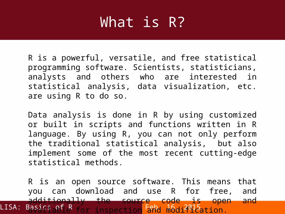
What is R?

R is a powerful, versatile, and free statistical programming software. Scientists, statisticians, analysts and others who are interested in statistical analysis, data visualization, etc. are using R to do so.

Data analysis is done in R by using customized or built in scripts and functions written in R language. By using R, you can not only perform the traditional statistical analysis, but also implement some of the most recent cutting-edge statistical methods.

R is an open source software. This means that you can download and use R for free, and additionally the source code is open and available for inspection and modification.

Why use R?


1. R is free and open.

2. R is a language. You learn much more than just point and click.

3. R has excellent tools for graphics and data visualization.

4. R is flexible. You are not restricted to the built-in functions; you can customize and extend those functions to serve your own needs.

You can make your analysis your own!


How to Obtain R for your own computer?

Windows:http://cran.r-project.org/bin/windows/base/

MacOs X:http://cran.r-project.org/bin/macosx/


R Studio

The console will display all your results and commands.

Workspace and history of

commands

Available files, generated plots, package

management and help

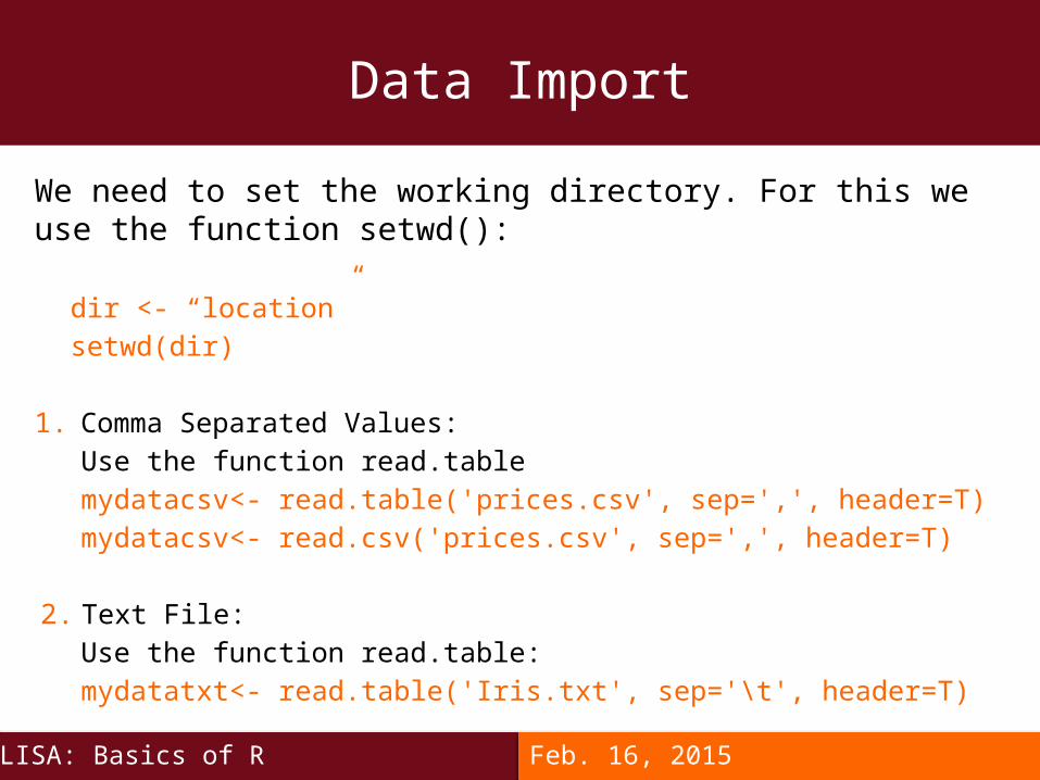
We need to set the working directory. For this we use the function setwd():

dir <- “location”

setwd(dir)

1. Comma Separated Values:

Use the function read.table

mydatacsv<- read.table('prices.csv', sep=',', header=T)

mydatacsv<- read.csv('prices.csv', sep=',', header=T)

2. Text File:

Use the function read.table:

mydatatxt<- read.table('Iris.txt', sep='\t', header=T)

Data Import


Data Structures and Manipulation

1. Object CreationExpression: A command is given, evaluated and the result is printed on the screen. Assignment: Storing the results of expressions.

2. Vectors:The basic data structure in R. (Scalars are vectors of dimension 1).a. Creating sequences:- : command. Creates a sequence incrementing/decrementing by 1 - seq() command.

b. Vectors with no pattern. c() function. c. Vectors of characters. Also use c() function with the help of “”d. Repeating values. rep() function. e. Arithmetic with vectors: All basic operations can be performed with

vectors. f. Subsets: The basic syntax for subsetting vectors is: vector[index]




3. Matrices: Objects in two dimensions.a. Creating Matrices

Command: matrix(data, nrow, ncol, byrow).data: list of elements that will fill the matrix.nrow, ncol: number of elements in the rows and the columns respectively.byrow: filling the matrix by row. The default is FALSE.

b. Some Matrix Functions• dim(): Lists the dimensions of the matrix.• cbind(): Creating matrix by putting columns together.• rbind(): Creating matrix by putting rows together. • diag(d): Creates identity matrix of dimension d.



c. Some Matrix computations• Addition • Subtraction• Inverse: function solve()• Transpose: function t()• Element-wise multiplication: *• Matrix multiplication: %*%

d. Subsets • Referencing a cell: matrix[r,c], where r represents the row and c

represents the column.• Referencing a row: matrix[r,]• Referencing a column: matrix[,c]

• The data are a random sample of records of re-sales of homes from Feb. 15 to Apr. 30, 1993 from the files maintained by the Albuquerque Board of Realtors. This type of data is collected by multiple listing agencies in many cities and is used by realtors as an information base.

• Number of cases: 65

• Variable Names: • PRICE = Selling price ($hundreds) • SQFT = Square feet of living space • AGE = Age of home (years) • NE = Located in northeast sector of city (=1) or not (=0)

Practice 1: Prices Data Set (prices.csv)


Lets review some of the matrix commands we learned previously by applying them to our new dataset.

1. What is the dimension of our dataset?

2. Assign the value of the cell [2,3] to the new variable var1

3. Assign the value of the cell [10,4] to the new variable var2

4. Output the value of each column separately.

5. Assign the values of SQFT to a new variable SQFT1.

6. Output the value of row 15.

Practice 1: Prices Data Set (prices.csv)


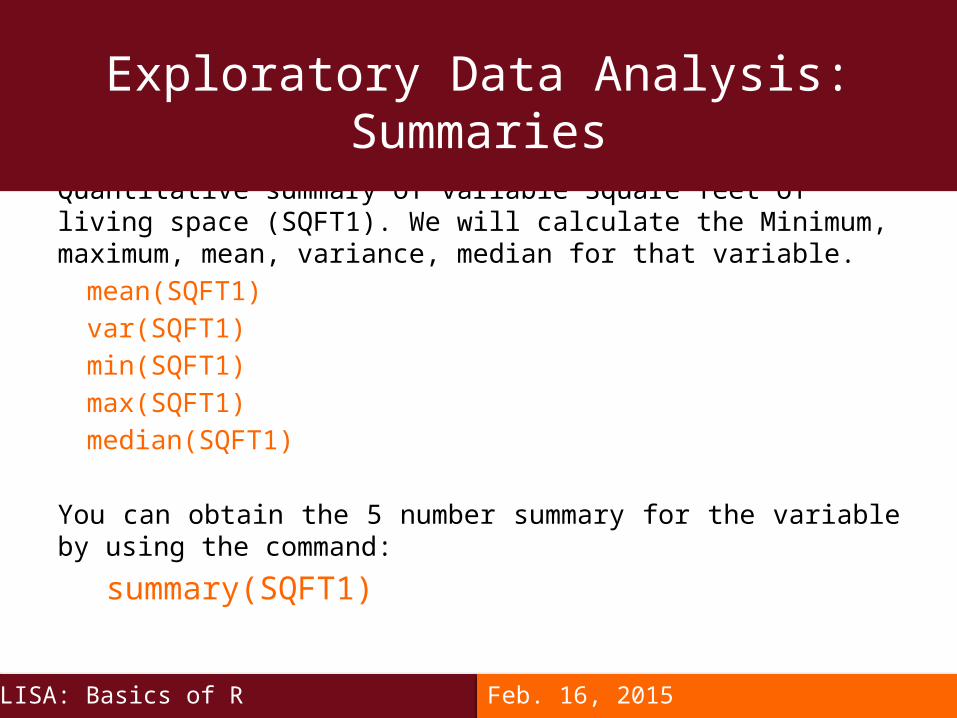
Quantitative summary of variable Square feet of living space (SQFT1). We will calculate the Minimum, maximum, mean, variance, median for that variable.

mean(SQFT1)

var(SQFT1)

min(SQFT1)

max(SQFT1)

median(SQFT1)

You can obtain the 5 number summary for the variable by using the command:

summary(SQFT1)

Exploratory Data Analysis: Summaries


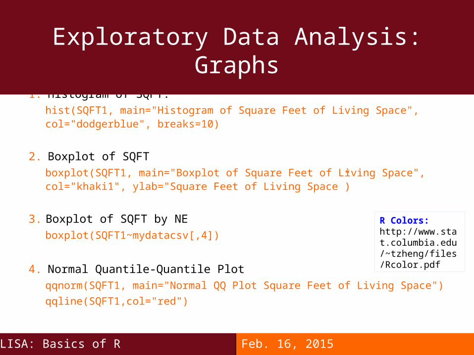
1. Histogram of SQFT.

hist(SQFT1, main="Histogram of Square Feet of Living Space", col="dodgerblue", breaks=10)

2. Boxplot of SQFT

boxplot(SQFT1, main="Boxplot of Square Feet of Living Space", col="khaki1", ylab="Square Feet of Living Space”)

3. Boxplot of SQFT by NE

boxplot(SQFT1~mydatacsv[,4])

4. Normal Quantile-Quantile Plot

qqnorm(SQFT1, main="Normal QQ Plot Square Feet of Living Space")

qqline(SQFT1,col="red")

Exploratory Data Analysis: Graphs


R Colors: http://www.stat.columbia.edu/~tzheng/files/Rcolor.pdf

This statement allows for code to be executed repeatedly.

for(i in 1:n){

statement

}

For Loops


This statement allows for code to be executed repeatedly while a condition holds true.

while(condition){

statement

}

While Loops


if statement - use this statement to execute some code only if a specified condition is true:

if(condition){ statement}

If/Else Statement


if...else statement - use this statement to execute some code if the condition is true and another code if the condition is false.

if ( condition )

statement

else

statement2

If/Else Statement


if...else if....else statement - use this statement to select one of many blocks of code to be executed

if (condition){

statement

} else{

if (condition2){

statement2

} else {

Statement4

}

}

If/Else Statement


If you have modified your dataset in R you can export it as a .csv file using the following code:

write.csv(mydatacsv,file="mydatacsv.csv")

Can also export vectors or other objects that you have created to .csv file:

write.csv(vec2,file="vec2.csv")

Data Export: .csv


If you have modified your dataset in R you can export it as a space delimited .txt file using the following code:

write.table(mydatacsv,file="mydatatxt.txt", sep=" ")

You can export it as a tab delimited .txt file using the following code:

write.table(mydatacsv,file="mydatatxt2.txt", sep="\t")

Data Export: .txt


• Point and Click at the interface and search.• Type ?word at the console and R will search for help

pages.• Google: How to do in R.• UCLA website: http://www.ats.ucla.edu/stat/

Help


http://www.ats.ucla.edu/stat/

The variable content for each record on the file includes demographic and socioeconomic variables from the Current Population Survey combined with the underlying cause of death mortality outcome and the follow-up time until death for records of the deceased or 11 years of follow-up for those not deceased.

The previous information was taken from the reference manual of the dataset, this manual and a complete variable description is uploaded in the course materials folder (Dataset reference manual.pdf).

Practice 2: National Longitudinal Mortality Study Dataset


1. Read into R the dataset pubfileb.csv.

2. Determine the dimensions of the dataset.

3. Extract the variable povpct, income as percent of poverty level (column 35) as a new variable.

4. Extract the variable ms, marital status (column 5) as a new variable.

5. Obtain the minimum, maximum, mean, variance, median for the variable povpct and store them in separate variables.

6. Create a vector with the stored values from 5.

7. Create a histogram of povpct of a different color with 20 breaks.

Practice 2-a: National Longitudinal Mortality Study Dataset


1. Create a boxplot of povpct of a different color.

2. Create a boxplot of povpct by ms with the same color for all boxes.

3. Create a boxplot of povpct by ms with the same color for the first

three boxes and another color for the remaining three boxes.

4. Create a normal Q-Q plot for povpct.

5. Using for loops count how many observations are there in a

metropolitan area (smsast=1) (col 20) with an age lower than 15

(col 2).

6. Export your extracted variables as a .csv file and the dataset as a

tab delimited .txt file.

Practice 2-b: National Longitudinal Mortality Study Dataset



Please fill the sign in sheet & complete the survey that will be sent to you by email.

Thank you!

Documents

LISA Short Course Series Basics of R Lin Zhang Feb. 16, 2015 LISA: Basics of RFeb. 16, 2015