LIS 7.1 Users’ Guide - NASA · 9.3.5 ANSA Snow Covered Fraction ... User’s Guide. This document de-scribes how to download and install the code and data needed to run the LIS

Land Information System

LIS 7.1 Users’ Guide

August 4, 2016

Revision 1.5

History:

Revision Summary of Changes Date1.5 Updates for LIS 7.1rp7 Public Release August 4, 2016

National Aeronautics and Space AdministrationGoddard Space Flight CenterGreenbelt, Maryland 20771

1

History:

Revision Summary of Changes Date1.4 LIS 7.1 AFWA FY15 Deliverable July 28, 20161.3 LIS 7.1rp1 Public Release December 15, 20151.2 Note unavailability of MERRA2 forcing data May 29, 20151.1 LIS 7.1 Public Release May 27, 20151.0 LIS 7.1 Initial AFWA Release April 13, 2015

2

Contents

1 Introduction 11

1.1 What’s New . . . . . . . . . . . . . . . . . . . . . . . . . . . . . . 11

1.1.1 LIS 7.1 . . . . . . . . . . . . . . . . . . . . . . . . . . . . 11

1.1.2 LIS 7.0 . . . . . . . . . . . . . . . . . . . . . . . . . . . . 12

1.1.3 LIS 6.2 . . . . . . . . . . . . . . . . . . . . . . . . . . . . 13

1.1.4 LIS 6.1 . . . . . . . . . . . . . . . . . . . . . . . . . . . . 14

1.1.5 LIS 6.0 . . . . . . . . . . . . . . . . . . . . . . . . . . . . 14

1.1.6 LIS 5.0 . . . . . . . . . . . . . . . . . . . . . . . . . . . . 15

1.1.7 LIS 4.2 . . . . . . . . . . . . . . . . . . . . . . . . . . . . 15

1.1.8 LIS 4.1 . . . . . . . . . . . . . . . . . . . . . . . . . . . . 16

1.1.9 LIS 4.0.2 . . . . . . . . . . . . . . . . . . . . . . . . . . . 16

1.1.10 LIS 4.0 . . . . . . . . . . . . . . . . . . . . . . . . . . . . 16

1.1.11 LIS 3.1 . . . . . . . . . . . . . . . . . . . . . . . . . . . . 16

1.1.12 LIS 3.0 . . . . . . . . . . . . . . . . . . . . . . . . . . . . 17

2 Background 18

2.1 LIS . . . . . . . . . . . . . . . . . . . . . . . . . . . . . . . . . . . 18

2.2 LIS core . . . . . . . . . . . . . . . . . . . . . . . . . . . . . . . . 19

3 Preliminary Information 21

4 Obtaining the Source Code 22

4.1 Important Note Regarding File Systems . . . . . . . . . . . . . . 22

3

4.2 Public Release Source Code Tar File . . . . . . . . . . . . . . . . 22

4.3 Checking Out the Source Code . . . . . . . . . . . . . . . . . . . 23

4.4 Source files . . . . . . . . . . . . . . . . . . . . . . . . . . . . . . 23

5 Building the Executable 33

5.1 Development Tools . . . . . . . . . . . . . . . . . . . . . . . . . . 33

5.2 Required Software Libraries . . . . . . . . . . . . . . . . . . . . . 33

5.3 Optional Software Libraries . . . . . . . . . . . . . . . . . . . . . 35

5.4 Build Instructions . . . . . . . . . . . . . . . . . . . . . . . . . . 38

5.5 Generating documentation . . . . . . . . . . . . . . . . . . . . . . 41

6 Running the Executable 42

6.1 Command line arguments . . . . . . . . . . . . . . . . . . . . . . 43

7 Test-cases 44

7.1 Public tests . . . . . . . . . . . . . . . . . . . . . . . . . . . . . . 44

7.1.1 The testcases Sub-directory . . . . . . . . . . . . . . . . . 44

7.1.2 Input and output data . . . . . . . . . . . . . . . . . . . . 45

7.2 Internal tests . . . . . . . . . . . . . . . . . . . . . . . . . . . . . 45

7.2.1 The testcases Sub-directory . . . . . . . . . . . . . . . . . 45

7.2.2 Test-cases LDT . . . . . . . . . . . . . . . . . . . . . . . . 46

7.2.3 Test-cases Input . . . . . . . . . . . . . . . . . . . . . . . 46

7.2.4 Test-cases Output . . . . . . . . . . . . . . . . . . . . . . 46

7.2.5 Output Example . . . . . . . . . . . . . . . . . . . . . . . 47

4

8 Output Data Processing 49

8.1 Fortran binary output format . . . . . . . . . . . . . . . . . . . . 50

8.2 GRIB1 output format . . . . . . . . . . . . . . . . . . . . . . . . 50

8.3 NetCDF output format . . . . . . . . . . . . . . . . . . . . . . . 50

9 LIS config File 51

9.1 Overall driver options . . . . . . . . . . . . . . . . . . . . . . . . 51

9.2 Runtime options . . . . . . . . . . . . . . . . . . . . . . . . . . . 56

9.3 Data assimilation . . . . . . . . . . . . . . . . . . . . . . . . . . . 63

9.3.1 AMSR-E (NASA) soil moisture assimilation . . . . . . . . 71

9.3.2 AMSR-E (LPRM) soil moisture assimilation . . . . . . . 72

9.3.3 ECV soil moisture assimilation . . . . . . . . . . . . . . . 72

9.3.4 WindSat soil moisture assimilation . . . . . . . . . . . . . 73

9.3.5 ANSA Snow Covered Fraction (SCF) Assimilation . . . . 74

9.3.6 MODIS snow cover fraction assimilation . . . . . . . . . . 76

9.3.7 PMW snow depth or SWE assimilation . . . . . . . . . . 76

9.3.8 GRACE TWS Assimilation . . . . . . . . . . . . . . . . . 80

9.3.9 SMOPS soil moisture assimilation . . . . . . . . . . . . . 81

9.4 Radiative Transfer/Forward Models . . . . . . . . . . . . . . . . 82

9.4.1 CRTM2EM . . . . . . . . . . . . . . . . . . . . . . . . . . 82

9.4.2 CMEM3 . . . . . . . . . . . . . . . . . . . . . . . . . . . . 84

9.5 Optimization and Uncertainty Estimation . . . . . . . . . . . . . 85

9.5.1 Least squares . . . . . . . . . . . . . . . . . . . . . . . . . 87

9.5.2 Probability . . . . . . . . . . . . . . . . . . . . . . . . . . 87

5

9.5.3 Likelihood . . . . . . . . . . . . . . . . . . . . . . . . . . . 87

9.5.4 Genetic Algorithm . . . . . . . . . . . . . . . . . . . . . . 87

9.5.5 Differential Evolution Markov Chain (DEMCz) algorithm 89

9.5.6 Monte Carlo simulation . . . . . . . . . . . . . . . . . . . 90

9.5.7 Observations for Parameter Estimation . . . . . . . . . . 90

9.5.8 AMSRE SR Emissivity . . . . . . . . . . . . . . . . . . . 90

9.5.9 AMSR-E (LPRM) pe soil moisture . . . . . . . . . . . . . 91

9.5.10 No obs . . . . . . . . . . . . . . . . . . . . . . . . . . . . . 91

9.6 Parameters . . . . . . . . . . . . . . . . . . . . . . . . . . . . . . 91

9.6.1 Parameter options . . . . . . . . . . . . . . . . . . . . . . 92

9.6.2 TBOT lag . . . . . . . . . . . . . . . . . . . . . . . . . . . 96

9.6.3 MODIS real-time LAI . . . . . . . . . . . . . . . . . . . . 97

9.6.4 NESDIS weekly greenness fraction . . . . . . . . . . . . . 97

9.6.5 SPORT greenness fraction . . . . . . . . . . . . . . . . . . 97

9.6.6 VIIRS greenness fraction . . . . . . . . . . . . . . . . . . 98

9.7 Forcings . . . . . . . . . . . . . . . . . . . . . . . . . . . . . . . . 99

9.7.1 GDAS . . . . . . . . . . . . . . . . . . . . . . . . . . . . . 99

9.7.2 GEOS . . . . . . . . . . . . . . . . . . . . . . . . . . . . . 99

9.7.3 ECMWF . . . . . . . . . . . . . . . . . . . . . . . . . . . 100

9.7.4 ECMWF Reanalysis . . . . . . . . . . . . . . . . . . . . . 100

9.7.5 PRINCETON . . . . . . . . . . . . . . . . . . . . . . . . . 100

9.7.6 Rhone AGG . . . . . . . . . . . . . . . . . . . . . . . . . . 100

9.7.7 GSWP2 . . . . . . . . . . . . . . . . . . . . . . . . . . . . 101

6

9.7.8 GMAO GLDAS . . . . . . . . . . . . . . . . . . . . . . . . 102

9.7.9 GFS . . . . . . . . . . . . . . . . . . . . . . . . . . . . . . 102

9.7.10 MERRA-Land . . . . . . . . . . . . . . . . . . . . . . . . 103

9.7.11 MERRA2 . . . . . . . . . . . . . . . . . . . . . . . . . . . 103

9.7.12 GSWP1 . . . . . . . . . . . . . . . . . . . . . . . . . . . . 104

9.8 Supplemental forcings . . . . . . . . . . . . . . . . . . . . . . . . 104

9.8.1 AGRMET radiation (latlon) . . . . . . . . . . . . . . . . 104

9.8.2 AGRMET radiation (polar stereographic) . . . . . . . . . 105

9.8.3 CMAP precipitation . . . . . . . . . . . . . . . . . . . . . 105

9.8.4 CEOP station data . . . . . . . . . . . . . . . . . . . . . . 105

9.8.5 SCAN station data . . . . . . . . . . . . . . . . . . . . . . 105

9.8.6 NLDAS1 . . . . . . . . . . . . . . . . . . . . . . . . . . . 106

9.8.7 NLDAS2 . . . . . . . . . . . . . . . . . . . . . . . . . . . 107

9.8.8 TRMM 3B42RT precipitation . . . . . . . . . . . . . . . . 108

9.8.9 TRMM 3B42V6 precipitation . . . . . . . . . . . . . . . . 109

9.8.10 TRMM 3B42V7 precipitation . . . . . . . . . . . . . . . . 109

9.8.11 CMORPH precipitation . . . . . . . . . . . . . . . . . . . 109

9.8.12 Stage II precipitation . . . . . . . . . . . . . . . . . . . . 110

9.8.13 Stage IV precipitation . . . . . . . . . . . . . . . . . . . . 110

9.8.14 NARR . . . . . . . . . . . . . . . . . . . . . . . . . . . . . 110

9.8.15 RFE2Daily . . . . . . . . . . . . . . . . . . . . . . . . . . 111

9.8.16 PET USGS . . . . . . . . . . . . . . . . . . . . . . . . . . 111

9.8.17 RFE2 data bias corrected to GDAS . . . . . . . . . . . . 111

7

9.8.18 NAM242 . . . . . . . . . . . . . . . . . . . . . . . . . . . 112

9.8.19 WRFout . . . . . . . . . . . . . . . . . . . . . . . . . . . . 112

9.8.20 GEOS5 Forecast . . . . . . . . . . . . . . . . . . . . . . . 112

9.8.21 GDAS for LSWG . . . . . . . . . . . . . . . . . . . . . . . 112

9.8.22 Bondville . . . . . . . . . . . . . . . . . . . . . . . . . . . 113

9.8.23 SNOTEL . . . . . . . . . . . . . . . . . . . . . . . . . . . 113

9.8.24 COOP . . . . . . . . . . . . . . . . . . . . . . . . . . . . . 114

9.8.25 VIC processed forcing . . . . . . . . . . . . . . . . . . . . 114

9.8.26 PALS station . . . . . . . . . . . . . . . . . . . . . . . . . 115

9.8.27 PILDAS . . . . . . . . . . . . . . . . . . . . . . . . . . . . 116

9.8.28 RDHM356 . . . . . . . . . . . . . . . . . . . . . . . . . . 116

9.9 Land surface models . . . . . . . . . . . . . . . . . . . . . . . . . 118

9.9.1 Forcing only – Template . . . . . . . . . . . . . . . . . . . 118

9.9.2 NCEP’s Noah-2.7.1 . . . . . . . . . . . . . . . . . . . . . . 118

9.9.3 NCAR’s Noah-3.2 . . . . . . . . . . . . . . . . . . . . . . 121

9.9.4 NCAR’s Noah-3.3 . . . . . . . . . . . . . . . . . . . . . . 124

9.9.5 NCAR’s Noah-3.6 . . . . . . . . . . . . . . . . . . . . . . 128

9.9.6 NoahMP 3.6 . . . . . . . . . . . . . . . . . . . . . . . . . 131

9.9.7 CLM 2.0 . . . . . . . . . . . . . . . . . . . . . . . . . . . . 138

9.9.8 VIC 4.1.1 . . . . . . . . . . . . . . . . . . . . . . . . . . . 139

9.9.9 VIC 4.1.2 . . . . . . . . . . . . . . . . . . . . . . . . . . . 140

9.9.10 Mosaic . . . . . . . . . . . . . . . . . . . . . . . . . . . . . 142

9.9.11 HySSiB . . . . . . . . . . . . . . . . . . . . . . . . . . . . 144

8

9.9.12 Catchment Fortuna-2 5 . . . . . . . . . . . . . . . . . . . 145

9.9.13 GeoWRSI 2.0 . . . . . . . . . . . . . . . . . . . . . . . . . 146

9.9.14 RDHM 3.5.6 . . . . . . . . . . . . . . . . . . . . . . . . . 147

9.10 Irrigation . . . . . . . . . . . . . . . . . . . . . . . . . . . . . . . 153

9.11 Routing . . . . . . . . . . . . . . . . . . . . . . . . . . . . . . . . 154

9.11.1 HYMAP routing . . . . . . . . . . . . . . . . . . . . . . . 154

9.11.2 NLDAS routing . . . . . . . . . . . . . . . . . . . . . . . . 156

9.12 Model output configuration . . . . . . . . . . . . . . . . . . . . . 157

9.13 Defining a time interval . . . . . . . . . . . . . . . . . . . . . . . 158

10 Specification of Input Forcing Variables 159

11 Model Output Specifications 161

12 User Support 168

12.1 Modeling Guru . . . . . . . . . . . . . . . . . . . . . . . . . . . . 168

12.2 Requesting help . . . . . . . . . . . . . . . . . . . . . . . . . . . . 168

A Frequently Asked Questions 169

B LIS Binary File Convention 170

B.1 Introduction . . . . . . . . . . . . . . . . . . . . . . . . . . . . . . 170

B.2 Byte order . . . . . . . . . . . . . . . . . . . . . . . . . . . . . . . 170

B.3 Storage organization . . . . . . . . . . . . . . . . . . . . . . . . . 170

B.4 Missing/undefined values . . . . . . . . . . . . . . . . . . . . . . 170

B.5 File name extension convention and access code samples . . . . . 171

9

C CSIRO Open Source Software License Agreement (variation ofthe BSD / MIT License) 172

10

1 Introduction

This is the Land Information System (LIS) User’s Guide. This document de-scribes how to download and install the code and data needed to run the LISexecutable for LIS revision 7.1. It describes how to build and run the code, andfinally this document also describes how to download output data-sets to usefor validation.

This document consists of 12 sections, described as follows:

1 Introduction: the section you are currently reading

2 Background: general information about the LIS project

3 Preliminary Information: general information, steps, instructions, anddefinitions used throughout the rest of this document

4 Obtaining the Source Code: the steps needed to download the sourcecode

5 Building the Executable: the steps needed to build the LIS executable

6 Running the Executable: the steps needed to prepare and submit arun, also describes the various run-time configurations

7 Test Cases: describes the LIS test cases.

8 Output Data Processing: the steps needed to post-process generatedoutput for visualization

9 LIS config File: describes the user-configurable options.

10 Specification of Input Forcing Variables: describes the user-configurableinput forcing variable options.

11 Model Output List Table: describes the user-configurable output vari-able options.

12 User Support:

1.1 What’s New

1.1.1 LIS 7.1

1. Includes Noah 3.6

2. Includes NoahMP 3.6

11

3. Includes CABLE 1.4b

4. Includes flood irrigation

5. Includes drip irrigation

6. Supports VIIRS Daily GVF data

7. Supports TRMM 3B42 V7 real time precipitation

8. Supports Gaussian T1534 GFS met forcing data

9. Supports MERRA-2 met forcing data — these data are not currentlyavailable to external users; they should become available in July 2015

10. Supports downscaling precipitation (PRISM) (NLDAS-2 only)

1.1.2 LIS 7.0

1. Requires companion Land Data Toolkit (LDT) input data and parameterpreprocessor

2. Includes VIC 4.1.2.l

3. Includes RDHM 3.5.6 (SacHTET and Snow17)

4. Includes demand sprinkler irrigation

5. Includes HYMAP routing

6. Includes NLDAS routing

7. Includes radiative transfer model support

• LIS-CRTM2EM — LIS’ implementation of JCSDA’s CRTM2 withemissivity support

See http://ftp.emc.ncep.noaa.gov/jcsda/CRTM/.

• LIS-CMEM3 — LIS’ implementation of ECMWF’s CMEM 3.0

See http://old.ecmwf.int/research/data assimilation/land surface/cmem/cmem source.htmlfor the original code.

8. Includes parameter and uncertainty estimation support

• Genetic algorithm (GA)

• Monte Carlo sampling (MCSIM)

• Differential evolution Markov chain z (DEMCz)

9. Supports ensemble of met forcing sources

10. Supports GEOS 5 forecast met forcing data

12

http://ftp.emc.ncep.noaa.gov/jcsda/CRTM/

http://old.ecmwf.int/research/data_assimilation/land_surface/cmem/cmem_source.html

11. Supports PALS met forcing data

12. Supports PILDAS met forcing data

13. Supports ECV soil moisture data assimilation

14. Supports GRACE data assimilation

15. Supports PMW snow data assimilation

16. Supports SMOPS soil moisture data assimilation

Note that the notion of a base forcing and a supplemental forcing have beenreplaced with the notion of a meteorological forcing. Thus the support in base-forcing and in suppforcing have been combined into metforcing.

Note that LIS is developing support for surface types other than land. Thus allthe land surface models contained in lsms have been moved into surfacemod-els/land.

Note that the companion program LDT is now required to process input pa-rameters. Thus the support for static and climatological parameters have beenremoved from params and placed into LDT.

1.1.3 LIS 6.2

1. Includes VIC 4.1.1.

2. Includes CABLE 1.4b — restricted distribution.

3. Includes Catchment F2.5.

4. Includes Noah 3.3.

5. Includes SiB2.

6. Includes WRSI.

7. Support for North American Mesoscale Forecast System (NAM)“242 AWIPS Grid – Over Alaska” product.

8. Support for USGS potential evapotranspiration (PET) data (for use inWRSI).

9. Support for Climate Prediction Center’s (CPC) Rainfall Estimates version2 (RFE2) daily precipition (for use in WRSI).

10. Support to apply lapse-rate correction to bottom temperature field (foruse in Noah).

13

1.1.4 LIS 6.1



3. Support for SPoRT Daily GVF data.

4. Support for North American Regional Reanalysis (3d) (NARR) data.

5. Support for NCEP’s modified IGBP MODIS landcover data.

6. Support to specify direction for output variables.

7. Support for assimilation of ANSA snow depth products, MODIS snow-cover, and LPRM retrievals of AMSRE soil moisture.

1.1.5 LIS 6.0

1. Modules have been restructured to streamline public and private interfaces

2. Restructured AGRMET processing—parallel support, lat/lon support.

3. This version now uses ESMF 3.1.0rp3.

4. Support for computational halos.

5. Allows mosaicing of different forcings concurrently (e.g. GDAS global +NLDAS over CONUS+SALDAS over south america, etc.)

6. Allows multiple overlays of different supplemental forcings (e.g. GDASoverlaid with NLDAS, AGRMET, STAGEIV)

7. Allows concurrent instances of data assimilation

8. Includes a highly configurable I/O interface (Allows unit conversions,temporal averaging, model-independent support for binary, Grib1 andNETCDF)

9. Includes support for 3d forcing (that includes the atmospheric profile) anda configurable specification of the forcing inputs

10. A dynamic bias estimation component (from NASA GMAO) has beenadded to the data assimilation subsystem.

11. Generic support for parameter estimation/optimization with the implmen-tation of a heuristic approach using Genetic Algorithms.

12. New sources for data assimilation (using NASA and NESDIS retrievals ofAMSRE soil moisture)

14

13. Support for real time GVF data from NESDIS and MODIS

14. A suite of upscaling algorithms to complement the existing spatial down-scaling algorithms.

15. Support for new map projections - UTM

16. Support for forward modeling using radiative transfer models, and supportfor radiance based assimilation

1.1.6 LIS 5.0

1. This version includes the infrastructure for performing data assimilationusing a number of different algorithms from simple approaches such asdirect insertion to the more sophisticated ensemble kalman filtering.

2. More streamlined support for different architectures: A configuration basedspecification for the LIS makefile.

3. The data assimilation infrastructure utilizes the Earth System ModelingFramework (ESMF) structures. The LIS configuration utility has beenreplaced with the corresponding ESMF utility.

1.1.7 LIS 4.2

1. Completed implementation of AGRMET processing algorithms

2. Ability to run on polar stereographic, mercator, lambert conformal, andlat/lon projections

3. Updated spatial interpolation tools to support the transformations to/fromthe above grid projections

4. Switched to a highly interactive configurations management from the for-tran namelist-based lis.crd style.

5. Streamlined error and diagnostic logging, in both sequential and parallelprocessing environments.

6. extended grib support; included the UCAR-based read-grib library

7. Support for new supplemental forcing analyses - Huffman, CMORPH

15

1.1.8 LIS 4.1

1. Preliminary AFWA support

2. Ability to run on a defined layout of processors.

3. Updates to plugins, preliminary implementation of alarms.

4. Definition of LIS specfic environment variables.

1.1.9 LIS 4.0.2

1. GSWP-2 support – LIS can now run GSWP-2 experiments. Currentlyonly CLM and Noah models have full support.

2. Updates to the 1km running mode.

3. Updates to the GDS running mode.

1.1.10 LIS 4.0

1. VIC 4.0.5 – LIS’ implementation of VIC has been reinstated.

1.1.11 LIS 3.1

1. New domain-plugin support – facilitates creating new domains.

2. New domain definition support – facilitates defining running domains.Sub-domain selection now works for both MPI-based and non MPI-basedruns.

3. New parameter-plugin support – facilitates adding new input parameterdata-sets.

4. New LIS version of ipolates – facilitates creating new domains and baseforcing data-sets.

5. Compile-time MPI support – MPI libraries are no longer required to com-pile LIS.

6. Compile-time netCDF support – netCDF libraries are no longer requiredto compile LIS.

7. New LIS time manager support – ESMF time manager was removed.ESMF libraries are not required in this version of LIS.

16

1.1.12 LIS 3.0

1. Running Modes – Now there is more than one way to run LIS. In additionto the standard MPI running mode, there are the GDS running mode andthe 1 km running mode.

2. Sub-domain Selection – Now you are no longer limited to global simu-lations. You may choose any sub-set of the global domain to run over.See Section 9 for more details. (This is currently only available for theMPI-based running mode.)

3. Plug-ins – Now it is easy to add new LSM and forcing data-sets into theLIS driver. See LIS’ Developer’s Guide for more details.

17

2 Background

This section provides some general information about the LIS project.

2.1 LIS

Land Information System (LIS) is a flexible land surface modeling and data as-similation framework developed with the goal to integrate satellite- and ground-based observational data products and advanced land surface modeling tech-niques to produce optimal fields of land surface states and fluxes. The LISinfrastructure provides the modeling tools to integrate these observations withmodel forecasts to generate improved estimates of land surface conditions suchas soil moisture, evaporation, snow pack, and runoff, at 1km and finer spa-tial resolutions and at one-hour and finer temporal resolutions. The fine scalespatial modeling capability of LIS allows it take advantage of the EOS-era obser-vations, such as MODIS leaf area index, snow cover, and surface temperature,at their full native resolution. LIS features a high performance and flexible de-sign, provides infrastructure for data integration and assimilation, and operateson an ensemble of land surface models (LSM) for extension over user-specifiedregional or global domains. LIS is designed using advanced software engineer-ing principles to enable reuse and community sharing of modeling tools, dataresources, and assimilation algorithms. The system is designed as an object-oriented framework, with abstractions defined for customization and extensionto different applications. These extensible interfaces allow the incorporationof new domains, LSMs, land surface parameters, meteorological inputs, dataassimilation and optimization algorithms. The extensible nature of these inter-faces and the component style specification of the system allow rapid prototyp-ing and development of new applications. These features enable LIS to serveboth as a Problem Solving Environment (PSE) for hydrologic research to enableaccurate global water and energy cycle predictions, and as a Decision SupportSystem (DSS) to generate useful information for application areas includingdisaster management, water resources management, agricultural management,numerical weather prediction, air quality and military mobility assessment.

LIS currently includes a comprehensive suite of subsystems to support uncou-pled and coupled land data assimilation. A schematic of the LIS frameworkwith the associated subsystems are shown in the Figure below. The LIS-LSMsubsystem, which is the core of LIS, supports high performance, interopera-ble and portable land surface modeling with a suite of community land surfacemodels and input data. Further, the LIS-LSM subsystem is designed to encap-sulate the land surface component of an Earth System model. The LIS-WRFsubsystem supports coupled land-atmosphere modeling through both one-wayand two-way coupling to the WRF atmospheric model, leading to a hydromete-

18

orological modeling capability that can be used to evaluate the impact of landsurface processes on hydrologic prediction. The Data Assimilation (LIS-DA)subsystem supports multiple data assimilation algorithms that are focused ongenerating improved estimates of hydrologic model states. Finally, the Opti-mization (LIS-OPT) subsystem supports a suite of advanced optimization anduncertainty modeling tools in LIS.

2.2 LIS core

The central part of LIS software system is the LIS core that controls programexecution. The LIS core is a model control and input/output system (consistingof a number of subroutines, modules written in Fortran 90 source code) thatdrives multiple offline one-dimensional LSMs. The one-dimensional LSMs suchas CLM and Noah, apply the governing equations of the physical processesof the soil-vegetation-snowpack medium. These land surface models aim tocharacterize the transfer of mass, energy, and momentum between a vegetatedsurface and the atmosphere. When there are multiple vegetation types inside agrid box, the grid box is further divided into “tiles”, with each tile representinga specific vegetation type within the grid box, in order to simulate sub-grid scalevariability.

The execution of the LIS core starts with reading in the user specifications,including the modeling domain, spatial resolution, duration of the run, etc.Section 6 describes the exhaustive list of parameters specified by the user. Thisis followed by the reading and computing of model parameters. The time loopbegins and forcing data is read, time/space interpolation is computed and mod-ified as necessary. Forcing data is used to specify the boundary conditions tothe land surface model. The LIS core applies time/space interpolation to con-vert the forcing data to the appropriate resolution required by the model. Theselected model is run for a vector of “tiles” and output and restart files arewritten at the specified output interval.

Some of the salient features provided by the LIS core include:

• Vegetation type-based “tile” or “patch” approach to simulate sub-gridscale variability.

• Makes use of various satellite and ground-based observational systems.

• Derives model parameters from existing topography, vegetation, and soilcoverages.

• Extensible interfaces to facilitate incorporation of new land surface models,forcing schemes.

19

• Uses a modular, object oriented style design that allows “plug and play”of different features by allowing user to select only the components ofinterest while building the executable.

• Ability to perform regional modeling (only on the domain of interest).

• Provides a number of scalable parallel processing modes of operation.

Please refer to the software design document for a detailed description of thedesign of LIS core. The LIS reference manual provides a description of theextensible interfaces in LIS. The “plug and play” feature of different componentsis described in this document.

20

3 Preliminary Information

This section provides some preliminary information to make reading this guideeasier.

Commands are written with a fixed-width font. E.g.:

% cd /path/to/LISv7.0

% ls

“. . . compiler flags, then run gmake.”

File names are written in italics. E.g.:

/path/to/LISv7.0/src

21

4 Obtaining the Source Code

This section describes how to obtain the source code needed to build the LISexecutable.

Beginning with LIS public release 7.1rp1, the LIS source code is available asopen source under the NASA Open Source Agreement (NOSA). Please see LIS’web-site for a copy of the NOSA.

Due to the history of LIS’ development, prior versions of the LIS source codemay not be freely distributed. That older source code is available only to U.S.government agencies or entities with a U.S. government grant/contract. LIS’web-site explains how qualified persons may request a copy of the older sourcecode.

4.1 Important Note Regarding File Systems

LIS is developed on Linux/Unix platforms. Its build process expects a casesensitive file system. Please make sure that you unpack and/or svn checkout

the LIS code into a directory within a case sensitive file system. In particular, ifyou are using LIS within a Linux-based virtual machine hosted on a Windows orMacintosh system, do not compile/run LIS from within a shared folder. Movethe LIS source code into a directory within the virtual machine.

4.2 Public Release Source Code Tar File

The LIS 7.1 source code is available for download as a tar-file from LIS’ web-site.All users are encouraged to fill in the Registration Form and join the mailinglist, both also accessible from LIS’ web-site. After downloading the LIS tar-file:

1. Create a directory to unpack the tar-file into. Let’s call it TOPLEVELDIR.

2. Place the tar-file in this directory.% mv LIS public release 7.1rp7.tar.gz TOPLEVELDIR

3. Go into this directory.% cd TOPLEVELDIR

4. Run gzip -dc LIS public release 7.1rp7.tar.gz | tar xf -

This command will unzip and untar the tar-file.

22

http://lis.gsfc.nasa.gov/






Note that the directory containing the LIS source code will be referred to as$WORKING throughout the rest of this document.

4.3 Checking Out the Source Code

The LIS source code is maintained in a Subversion repository. Due to severalU.S. government restrictions, only the LIS development team and select col-laborators may have access to the repository. Those developers must use theSubversion client (svn) to obtain the LIS source code. If you need any helpregarding Subversion, please go to http://subversion.apache.org/.

For those granted access to the LIS source code repository:

1. Create a directory to checkout the code into. Let’s call it TOPLEVELDIR.

2. Go into this directory.% cd TOPLEVELDIR

3. Check out the source code into a directory called src.

For the public version, run the following command:

% svn checkout https://progress.nccs.nasa.gov/svn/lis/7/public7.1

src

Note that the directory containing the LIS source code will be referred to as$WORKING throughout the rest of this document.

4.4 Source files

Checking out the LIS source code (according the instructions in Section 4) willcreate a directory named src. The structure of src is as follows:

• archDirectory containing the configurable options for building the LIS exe-cutable

• configssome sample LIS configuration files

• corecore routines in LIS

23

http://subversion.apache.org/

• dataassimTop level directory for data assimilation support, which includes the fol-lowing subcomponents

– algorithmDirectory containing the following data assimilation algorithm im-plementations:

∗ didirect insertion algorithm for data assimilation

∗ enkfNASA GMAO’s Ensemble Kalman Filter algorithm for data as-similation

∗ enkfgraceGRACE Ensemble Kalman Filter algorithm for data assimilation

– biasEstimationDirectory containing the following dynamic bias estimation algo-rithms:

∗ gmaoBENASA GMAO’s dynamic bias estimation algorithm

– obsDirectory containing the following observation handlers for data as-similation:

∗ ANSA SCFBlended snow cover fraction from the AFWA NASA snow algo-rithm

∗ ECV smECV soil moisture

∗ GRACEGRACE soil moisture

∗ LPRM AMSREsmSoil moisture retrievals from AMSRE derived using the land pa-rameter retrieval model (LPRM) from University of Amsterdam

∗ MODISscaMODIS snow cover area product in HDF4/HDFEOS format

∗ NASA AMSREsmNASA AMSRE soil moisture data in binary format

∗ PMW snowPMW snow

∗ RT SMOPSsmSMOPS real time soil moisture

∗ WindSat smX-band soil moisture retrievals from WindSat

24

– perturbDirectory containing the following perturbation algorithm implemen-tations

∗ gmaopertNASA GMAO’s perturbation algorithm

• domains Directory containing the domains in the following map projec-tions / custom grids

– UTMUniversal Transverse Mercator grids

– hrapHydrologic Rainfall Analysis Project polar stereographic grid

– lambertLambert conformal grids

– latlonEquidistant cylindrical grids

– mercMercator grids

– polarPolar stereographic grids

• interpGeneric spatial and temporal interpolation routines

• irrigationDirectory containing the following irrigation schemes

– dripDrip irrigation scheme

– floodFlood irrigation scheme

– sprinklerDemand sprinkler irrigation scheme

• libDirectory contains the following RTM-related libraries

– lis-cmem3

– lis-crtm

– lis-crtm-profile-utility

• makeMakefile and needed header files for building LIS executable

25

• metforcingTop level directory for base meteorological forcing methods, which includesthe following implementations

– 3B42RTRoutines for handling the TRMM 3B42RT precipitation product

– 3B42RTV7Routines for handling the TRMM 3B42RTV7 precipitation product

– 3B42V6Routines for handling the TRMM 3B42V6 precipitation product

– 3B42V7Routines for handling the TRMM 3B42V7 precipitation product

– BondvilleRoutines for handling the Bondville forcing products

– PALSmetdataRoutines for handling the PALS station data

– PILDASRoutines for handling the PILDAS metforcing data

– RFE2DailyRoutines for handling the RFE2 precipitation product from FEWS-NET (diurnally non-disaggregated)

– RFE2gdasRoutines for handling the RFE2 precipitation product from FEWS-NET bias corrected against GDAS data

– WRFoutRoutines for handling WRF output as forcing input

– agrradRoutines for handling the AGRMET radiation product

– agrradpsRoutines for handling the AGRMET radiation product (polar stere-ographic prjection)

– ceopRoutines for handling the CEOP meteorological station data

– cmapRoutines for handling the CMAP precipitation product

– cmorphRoutines for handling the CMORPH precipitation product

– coopRoutines for handling the COOP precipitation product

– ecmwfECMWF meteorological forcing data

26

– ecmwfreanalECMWF reanalysis meteorological forcing data based on [1].

– gdasNCEP GDAS meteorological forcing data

– gdasLSWGGDAS profile data from the PMM land surface working group

– gdasT1534NCEP GDAS GFS T1534 meteorological forcing data

– geosNASA GEOS meteorological forcing data

– geos5fcstNASA GEOS 5 meteorological forecast forcing data

– gfsNCEP GFS meteorological forcing data

– gldasNASA GMAO GLDAS meteorological forcing data

– gswp1Global Soil Wetness Project-1 meteorological forcing data

– gswp2Global Soil Wetness Project-2 meteorological forcing data

– merra-landGMAO Modern Era Retrospective-Analysis for Research and Appli-cations data

– merra2GMAO Modern Era Retrospective-Analysis for Research and Appli-cations data

– nam242Routines for handling the North American Mesoscale Forecast Sys-tem (NAM) 242 AWIPS Grid – Over Alaska product

– narrRoutines for handling the North American Regional Reanalysis (3d)data

– nldas1Routines for handling the North American Land Data AssimilationSystem forcing product

– nldas2Routines for handling the North American Land Data AssimilationSystem 2 forcing product

– pet usgsRoutines for handling daily potential evapotranspiration data fromthe USGS FAO-PET method, using GDAS forcing fields as inputs

27

– princetonRenalaysis product from Princeton University ([3])

– rdhm356Routines for handling NOAA OHD RDHM 3.5.6 forcing data

– rhoneAGGRhone-AGG meteorological forcing data

– scanRoutines for handling the Soil Climate Analysis Network precipita-tion product

– snotelSNOTEL meteorological forcing data

– stg2Routines for handling the NCEP Stage IV QPE precipitation product

– stg4Routines for handling the NCEP Stage II precipitation product

– templateMetForcAn empty template for meteorological forcing data implementations

– vicforcingRoutines for handling VIC 4.1.1 pre-processed meteorological forcingdata

– vicforcing.4.1.2Routines for handling VIC 4.1.2 pre-processed meteorological forcingdata

• offlineContains the main program for the offline mode of operation

• optUETop level directory for optimization support, which includes the followingsubcomponents

– algorithmDirectory containing the following optimization algorithm implemen-tations

∗ DEMCzdifferential evolution monte carlo Z algorithm

∗ GASingle objective Genetic Algorithm

∗ MCSIMmonte carlo simple propagation scheme

– type

∗ paramestimDirectory for parameter estimation support

28

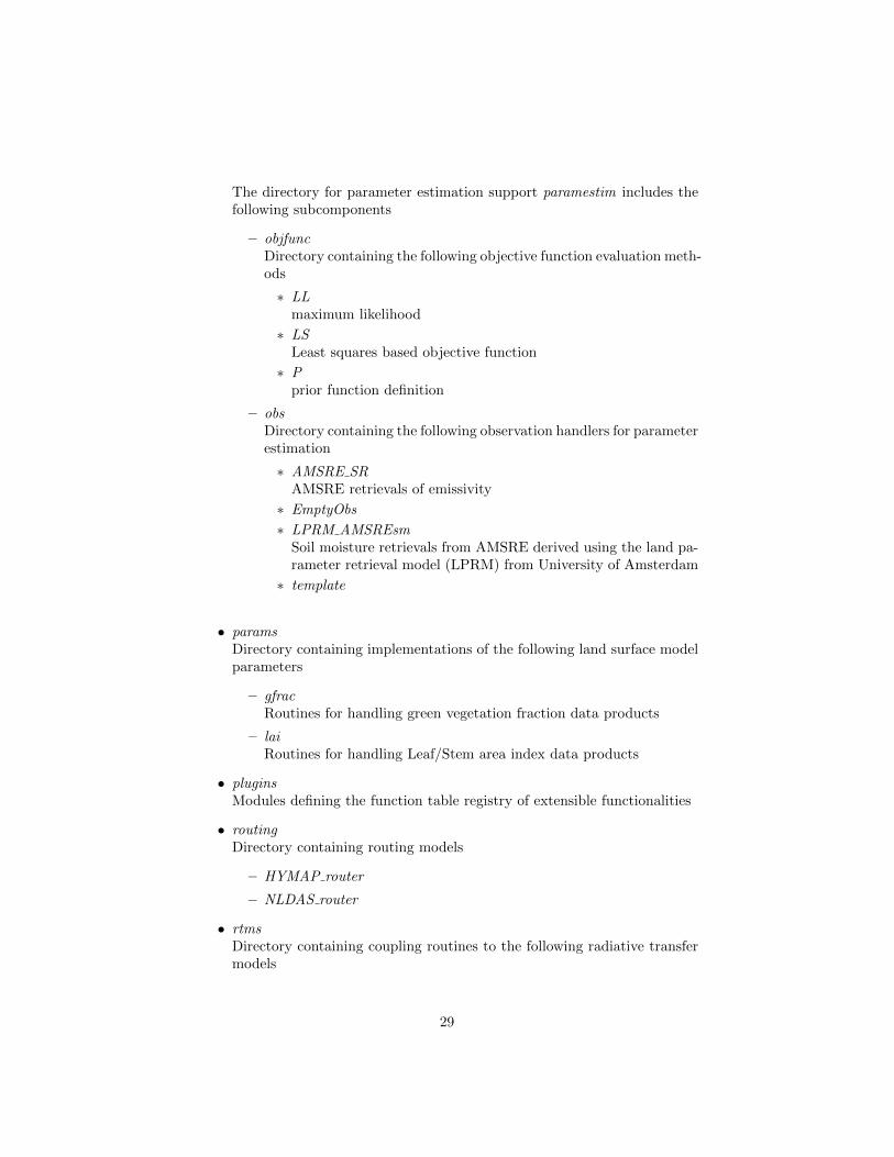
The directory for parameter estimation support paramestim includes thefollowing subcomponents

– objfuncDirectory containing the following objective function evaluation meth-ods

∗ LLmaximum likelihood

∗ LSLeast squares based objective function

∗ Pprior function definition

– obsDirectory containing the following observation handlers for parameterestimation

∗ AMSRE SRAMSRE retrievals of emissivity

∗ EmptyObs

∗ LPRM AMSREsmSoil moisture retrievals from AMSRE derived using the land pa-rameter retrieval model (LPRM) from University of Amsterdam

∗ template

• paramsDirectory containing implementations of the following land surface modelparameters

– gfracRoutines for handling green vegetation fraction data products

– laiRoutines for handling Leaf/Stem area index data products

• pluginsModules defining the function table registry of extensible functionalities

• routingDirectory containing routing models

– HYMAP router

– NLDAS router

• rtmsDirectory containing coupling routines to the following radiative transfermodels

29

– CMEM3Community Microwave Emission Model from ECMWF

– CRTM2EMRoutines to handle coupling to the JCSDA Community RadiativeTransfer Model Emissions model

• runmodesDirectory containing the following running modes in LIS

– paramEstimationRoutines to manage the program flow in the parameter estimationmode

– retrospectiveRoutines to manage the program flow in the retrospective analysismode

– smootherDARoutines to manage the program flow in the smoother da analysismode

– wrf cpl modeRoutines to manage the program flow in the coupled LIS-WRF modenot using ESMF

• surfacemodelsTop level directory for surface model support, which includes the followingsubcomponents

– landDirectory containing implementations of the following land surfacemodels

∗ cableCSIRO Atmosphere Biosphere Land Exchange model, version1.4b

∗ clm2NCAR community land model, version 2.0

∗ clsm.f2.5NASA GMAO Catchment land surface model version Fortuna2.5

∗ geowrsi.2GeoWRSI version 2

∗ hyssibNASA HySSIB land surface model

∗ mosaicNASA Mosaic land surface model

∗ noah.2.7.1NCEP Noah land surface model version 2.7.1

30

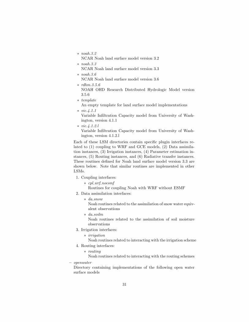
∗ noah.3.2NCAR Noah land surface model version 3.2



∗ rdhm.3.5.6NOAH OHD Research Distributed Hydrologic Model version3.5.6

∗ templateAn empty template for land surface model implementations

∗ vic.4.1.1Variable Infiltration Capacity model from University of Wash-ington, version 4.1.1

∗ vic.4.1.2.lVariable Infiltration Capacity model from University of Wash-ington, version 4.1.2.l

Each of these LSM directories contain specific plugin interfaces re-lated to (1) coupling to WRF and GCE models, (2) Data assimila-tion instances, (3) Irrigation instances, (4) Parameter estimation in-stances, (5) Routing instances, and (6) Radiative transfer instances.These routines defined for Noah land surface model version 3.3 areshown below. Note that similar routines are implemented in otherLSMs.

1. Coupling interfaces:

∗ cpl wrf noesmfRoutines for coupling Noah with WRF without ESMF

2. Data assimilation interfaces:

∗ da snowNoah routines related to the assimilation of snow water equiv-alent observations

∗ da soilmNoah routines related to the assimilation of soil moistureobservations

3. Irrigation interfaces:

∗ irrigationNoah routines related to interacting with the irrigation scheme

4. Routing interfaces:

∗ routingNoah routines related to interacting with the routing schemes

– openwaterDirectory containing implementations of the following open watersurface models

31

∗ templateAn empty template for open water surface model implementa-tions

• testcasestestcases for verifying various functionalities

• utilsMiscellaneous helpful utilities

Source code documentation may be found on LIS’ web-site. Follow the “Docu-mentation” link.

32


5 Building the Executable

This section describes how to build the source code and create LIS’executable — named LIS.

Please see Section 4.1 for information regarding using a case sensitve file systemfor compiling/running LIS.

5.1 Development Tools

This code has been compiled and run on Linux PC (Intel/AMD based) systemsand Cray systems. These instructions expect that you are using such a system.In particular you need:

• Linux

– Compilers

∗ either Intel Fortran Compiler version 13 (13.1.3.192 or higher)with corresponding Intel C Compiler

Note that LIS has been tested specifically with Intel compilers13.1.3.192, 14.0.3.174, and 15.1.133.

∗ or GNU’s Compiler Collection 4.9.2, both gfortran and gcc

– GNU’s make, gmake, version 3.77 or 3.81

• Cray/Linux

– Intel Fortran Compiler version 15.0.2 (or higher) with correspondingIntel C Compiler

– GNU’s make, gmake, version 3.77

5.2 Required Software Libraries

In order to build the LIS executable, the following libraries must be installedon your system:

• Earth System Modeling Framework (ESMF) version 5.2.0rp3 (or higher).(http://www.earthsystemmodeling.org/download/releases.shtml)

33

http://www.earthsystemmodeling.org/download/releases.shtml

Please read the ESMF User’s Guide for details on installing ESMF withMPI support and without MPI support (“mpiuni”).

Note that starting with ESMF version 5, the ESMF development team istrying to maintain backwards compatibility with its subsequent releases.The LIS development team, however, has neither compiled nor testedagainst versions of ESMF newer than 5.2.0rp3.

• JasPer version 1.900.1.(http://www.ece.uvic.ca/˜frodo/jasper/).

Note that when running the configure command you must include the--enable-shared option.

• GRIB-API version 1.12.3 (or higher).(https://software.ecmwf.int/wiki/display/GRIB/Home)

• NetCDF either version 3.6.3 or version 4.3.0 (or higher).(http://www.unidata.ucar.edu/software/netcdf/)

Please read the on-line documentation for details on installing NetCDF.

Additional notes for NetCDF 4:

– You must also choose whether to compile with compression enabled.Compiling with compression enabled requires HDF 5 and zlib li-braries. To enable compression, add --enable-netcdf-4 to theconfigure options. To disable compression, add --disable-netcdf-4

to the configure options.

An example of installing NetCDF 4 without compression:

% ./configure --prefix=$HOME/local/netcdf-4.3.0 --disable-netcdf-4

% gmake

% gmake install

An example of installing NetCDF 4 with compression:

% CPPFLAGS=-I$HOME/local/hdf5/1.8.11/include \> LDFLAGS=-L$HOME/local/hdf5/1.8.11/lib \> ./configure --prefix=$HOME/local/netcdf/4.3.0 --enable-netcdf-4

% gmake

% gmake install

– You must also download the netcdf-fortran-4.2.tar.gz file. First in-stall the NetCDF C library, then install the NetCDF Fortran library.Again, please read the on-line documentation for more details.

An example of installing the NetCDF 4 Fortran library:

% LD LIBRARY PATH=$HOME/local/netcdf/4.3.0/lib:$LD LIBRARY PATH \> CPPFLAGS=-I$HOME/local/netcdf/4.3.0/include \> LDFLAGS=-L$HOME/local/netcdf/4.3.0/lib \

34

http://www.ece.uvic.ca/~frodo/jasper/

https://software.ecmwf.int/wiki/display/GRIB/Home

http://www.unidata.ucar.edu/software/netcdf

> ./configure --prefix=$HOME/local/netcdf/4.3.0

% gmake

% gmake install

5.3 Optional Software Libraries

The following libraries are not required to compile LIS. They are used to extendthe functionality of LIS.

• Message Passing Interface (MPI)

If you wish to run LIS with multiple processes (i.e., in parallel), then youmust install an MPI library package.

– vendor supplied (e.g., Intel MPI) or

– MPICH version 1.2.7p1 (http://www-unix.mcs.anl.gov/mpi/mpich1/)

– Open MPI (http://www.open-mpi.org/)

Note that LIS does not support OpenMP style parallelization. There issome experimental support within LIS, but you should not enable it.

• HDF

You may choose either HDF version 4, HDF version 5, or both.

HDF is used to support a number of remote sensing datasets.

If you wish to use MODIS snow cover area observations or NASA AMSR-Esoil moisture observations, then you need HDF 4 support.

If you wish to use ANSA snow cover fraction observations, then you needHDF 5 support.

If you wish to use PMW snow observations, then you need both HDF 4and HDF 5 support.

– HDF 4

If you choose to have HDF version 4 support, please download theHDF source for version 4.2r4 (or later) from (http://www.hdfgroup.org/products/hdf4)and compile the source to generate the HDF library. Make sure thatyou configure the build process to include the Fortran interfaces byadding the --enable-fortran option to the configure command.

Note that HDF4 contains its own embedded version of NetCDF. Youmust disable this support by adding the --disable-netcdf optionto the configure command.

Note that when compiling LIS with HDF 4 support, you must alsodownload and compile HDF-EOS2 (http://hdfeos.org/).

35

http://www-unix.mcs.anl.gov/mpi/mpich1/

http://www.open-mpi.org/

http://www.hdfgroup.org/products/hdf4

http://hdfeos.org/

– HDF 5

If you choose to have HDF version 5 support, please download theHDF source for version 1.8.11 (or later) from (http://www.hdfgroup.org/HDF5/)and compile the source to generate the HDF library. Make sure thatyou configure the build process to include the Fortran interfaces byadding the --enable-fortran option to the configure command.

• JCSDA CRTM version 2.0.2

If you wish to enable LIS’ RTM support, then you must install the CRTMlibrary from the Joint Centers for Satellite Data Assimilation (JCSDA).First go to http://ftp.emc.ncep.noaa.gov/jcsda/CRTM/Repository/ andfill out the CRTM.Subversion Account Request.pdf form. Once you haveaccess to their Subversion repository, checkout revision 9604 of the trunk.

Please create a directory outside of the LIS source code to checkout theCRTM library into. Then, within that new directory, run:

% svn checkout -r 9604 https://svnemc.ncep.noaa.gov/projects/crtm/trunk

Then you must copy the LIS specific updates into this checked out CRTMcode. See $WORKING/lib/lis-crtm/README.

Next compile and install the CRTM library:

% source Set CRTM Environment.sh

% cd src

% source configure/ifort.setup

Of course, choose the setup script that is appropriate for your envi-ronment.

% gmake

% gmake install

• LIS-CMEM library

If you wish to enable LIS’ RTM support, then you must manually compilean included library.

% cd $WORKING/lib/lis-cmem3

% gmake

• LIS-CRTM-PROFILE-UTILITY library

If you wish to enable LIS’ RTM support, then you must manually compilean included library.

% cd $WORKING/lib/lis-crtm-profile-utility

% gmake

% gmake install

36

http://www.hdfgroup.org/HDF5/

To install these libraries, follow the instructions provided at the various URLlisted above. These optional libraries have their own dependencies, which shouldbe documented in their respective documentation.

Please note that your system may have several different compilers installed.You must verify that you are building these libraries with the correct compiler.You should review the output from the configure, make, etc. commands. Ifthe wrong compiler is being used, you may have to correct your $PATH environ-ment variable, or set the $CC and $FC environment variables, or pass additionalsettings to the configure scripts. Please consult the installation instructionsprovided at the various URL listed above for each library.

If you wish to install all the libraries (required and optional, excluding JCSDACRTM, LIS-CMEM, and LIS-CRTM-PROFILE-UTILITY), here is the recom-mended order:

1. HDF 5 (optional)NetCDF has an optional dependency on HDF 5.

2. NetCDF (required)ESMF has an optional dependency on NetCDF.GRIB-API has an optional dependency on NetCDF.

3. JasPer (required)GRIB-API depends on JasPer.

4. GRIB-API (required)

5. MPI (optional)ESMF has an optional dependency on MPI.

6. ESMF (required)

7. HDF 4 (optional)HDF-EOS2 depends on HDF 4.

8. HDF-EOS2 (optional)

Note that due to the mix of programing languages (Fortran and C) used by LIS,you may run into linking errors when building the LIS executable. This is oftendue to (1) the Fortran compiler and the C compiler using different cases (uppercase vs. lower case) for external names, and (2) the Fortran compiler and Ccompiler using a different number of underscores for external names.

When compiling code using Absoft’s Pro Fortran SDK, set the following com-piler options:

37

-YEXT NAMES=LCS -s -YEXT SFX= -YCFRL=1

These must be set for each of the above libraries.

5.4 Build Instructions

1. Perform the steps described in Section 4 to obtain the source code.

2. Goto the $WORKING directory. This directory contains two scripts forbuilding the LIS executable: configure and compile.

3. Set the LIS ARCH environment variable based on the system you areusing. The following commands are written using Bash shell syntax.

• For a Linux system with the Intel Fortran compiler% export LIS ARCH=linux ifc

• For a Linux system with the GNU Fortran compiler% export LIS ARCH=linux gfortran

It is suggested that you place this command in your .profile (or equivalent)startup file.

4. Run the configure script first by typing:

% ./configure

This script will prompt the user with a series of questions regarding sup-port to compile into LIS, requiring the user to specify the locations ofthe required and optional libraries via several LIS specific environmentvariables. The following environment variables are used by LIS.

Variable Description UsageLIS FC Fortran 90 compiler requiredLIS CC C compiler requiredLIS MODESMF path to ESMF module files requiredLIS LIBESMF path to ESMF library files requiredLIS JASPER path to JasPer library requiredLIS GRIBAPI path to GRIB-API library requiredLIS NETCDF path to NetCDF library requiredLIS HDF4 path to HDF4 library optionalLIS HDF5 path to HDF5 library optionalLIS HDFEOS path to HDFEOS library optionalLIS MINPACK path to MINPACK library optionalLIS CRTM path to CRTM library optionalLIS CRTM PROF path to LIS-CRTM Profile library optionalLIS CMEM path to LIS-CMEM library optional

38

Note that the CC variable must be set to a C compiler, not a C++ compiler.A C++ compiler may mangle internal names in a manner that is notconsistent with the Fortran compiler. This will cause errors during linking.

It is suggested that you add these definitions to your .profile (or equivalent)startup file.

You may encounter errors either when trying to compile LIS or when tryingto run LIS because the compiler or operating system cannot find these li-braries. To fix this, you must add these libraries to your $LD LIBRARY PATH

environment variable. For example, say that you are using ESMF, GRIB-API, NetCDF, and HDF5. Then you must execute the following command(written using Bash shell syntax):

% export LD LIBRARY PATH=$LIS HDF5/lib:$LIS LIBESMF:$LIS NETCDF/lib:$LIS GRIBAPI/lib:$LD LIBRARY PATH

It is also suggested that you add this command to your .profile (or equiv-alent) startup file.

5. An example execution of the configure script is shown below:

sh$ ./configure

------------------------------------------------------------------------

Setting up configuration for LIS version 7.0...

Parallelism (0-serial, 1-dmpar, default=1):

Use openMP parallelism (1-yes, 0-no, default=0):

Optimization level (-2=strict checks, -1=debug, 0,1,2,3, default=2):

Assume little/big_endian data format (1-little, 2-big, default=2):

Use GRIBAPI? (1-yes, 0-no, default=1):

Enable AFWA-specific grib configuration settings? (1-yes, 0-no, default=0):

Use NETCDF? (1-yes, 0-no, default=1):

NETCDF version (3 or 4, default=4):

NETCDF use shuffle filter? (1-yes, 0-no, default = 1):

NETCDF use deflate filter? (1-yes, 0-no, default = 1):

NETCDF use deflate level? (1 to 9-yes, 0-no, default = 9):

Use HDF4? (1-yes, 0-no, default=1):

Use HDF5? (1-yes, 0-no, default=1):

Use HDFEOS? (1-yes, 0-no, default=1):

Use MINPACK? (1-yes, 0-no, default=0):

Use LIS-CRTM? (1-yes, 0-no, default=0):

Use LIS-CMEM? (1-yes, 0-no, default=0):

-----------------------------------------------------

configure.lis file generated successfully

-----------------------------------------------------

Settings are written to configure.lis in the make directory

If you wish to change settings, please edit that file.

To compile, run the compile script.

------------------------------------------------------------------------

39

At each prompt, select the desired value. If you desire the default value,then you may simply press the Enter key.

Most of the configure options are be self-explanatory. Here are a fewspecific notes:

• for Parallelism (0-serial, 1-dmpar, default=1):, dmpar refersto enabling MPI

• for Use openMP parallelism (1-yes, 0-no, default=0):, selectthe default value of 0. OpenMP support is experimental. Please donot use.

• for Assume little/big endian data format (1-little, 2-big,

default=2):, select the default value of 2. By default, LIS reads andwrites binary data in the big endian format. Only select the valueof 1, if you have reformatted all required binary data into the littleendian format.

• for Use GRIBAPI? (1-yes, 0-no, default=1):, select the defaultvalue of 1. Technically, GRIB support is not required by LIS; how-ever, most of the commonly used met forcing data are in GRIB,making GRIB support a practical requirement.

• for Use LIS-CRTM? (1-yes, 0-no, default=0):, if you wish to en-able LIS-CRTM2EM support, then you must also enable LIS-CMEMsupport. So for Use LIS-CMEM? (1-yes, 0-no, default=0):, youmust also select 1.

• for Use LIS-CMEM? (1-yes, 0-no, default=0):, if you wish to en-able LIS-CMEM support, then you must also enable LIS-CRTM. Sofor Use LIS-CRTM? (1-yes, 0-no, default=0):, you must also se-lect 1.

Note that due to an issue involving multiple definitions within the NetCDF3 and HDF 4 libraries, you cannot compile LIS with support for bothNetCDF 3 and HDF 4 together.

Note that if you compiled NetCDF 4 without compression, then whenspecifying NETCDF version (3 or 4, default=4):, select 3. Then youmust manually append -lnetcdff to the LDFLAGS variable in the make/configure.lisfile.

6. Compile the LIS source code by running the compile script.

% ./compile

This script will compile the libraries provided with LIS, the dependencygenerator and then the LIS source code. The executable LIS will be placedin the $WORKING directory upon successful completion of the compilescript.

7. Finally, copy the LIS executable into your running directory, $RUNNING.

40

5.5 Generating documentation

LIS code uses the ProTex (http://gmao.gsfc.nasa.gov/software/protex/) docu-menting system [2]. The documentation in LATEX format can be produced byusing the doc.sh in the $WORKING/utils directory. This command producesdocumentation, generating a number of LATEX files. These files can be easilyconverted to pdf using utilites such as pdflatex.

41

http://gmao.gsfc.nasa.gov/software/protex/

6 Running the Executable

This section describes how to run the LIS executable.

First you should create a directory to run LIS in. It is suggested that yourun LIS in a directory that is separate from your source code. This runningdirectory shall be referred to as $RUNNING. Next, copy the LIS executableinto your running directory.

% cp $WORKING/LIS $RUNNING

The single-process version of LIS is executed by the following command issuedin the $RUNNING directory.

% ./LIS

Note that when using the Lahey Fortran compiler, you must issue this commandto run the single-process version of LIS:

% ./LIS -Wl,T

The parallel version of LIS must be run through an mpirun script or similarmechanism. Assuming that MPI is installed correctly, the LIS simulation iscarried out by the following command issued from in the $RUNNING directory.

% mpirun -np N ./LIS

The -np N flag indicates the number of processes to use in the run, where youreplace N with the number of processes to use. On a multiprocessor machine,the parallel processing capbabilities of LIS can be exploited using this flag.

Some systems require that you submit your job into a batch queue. Pleaseconsult with your system adminstrator for instructions on how to do this.

Note that before running LIS, you must set your environment to have an un-limited stack size. For the Bash shell, run

% ulimit -s unlimited

To customize your run, you must modify the lis.config configuration file. SeeSection 9 for more information.

42

6.1 Command line arguments

LIS [-f <file> | --file <file>]

-f <file>, --file <file> specifies the name of the LIS run-time configuration file.By default, LIS expects the run-time configuration options to be definedin a file named lis.config. Use this command line argument to specify analternate run-time configuration file.

43

7 Test-cases

This section describes how to obtain and how to use the test-cases provided bythe LIS team.

There are two categories of testcases: public tests and internal tests.

7.1 Public tests

These test-cases are provided for the general LIS user to run. They help demon-strate a successful installation of LIS and its required libraries. They alsodemonstrate how to configure several different use-cases of LIS. These test-cases are comprised of three parts: a testcases sub-directory included in the LISsource code, input data, and output data.

7.1.1 The testcases Sub-directory

The public test-cases are contained within the src/testcases/public directory.The available tests are:

NLDAS2-a NLDAS domain + NLDAS-2 forcing + Noah-3.3 LSM + NLDASrouter or HYMAP router + AMSR-E DA soil moisture

NLDAS2-b NLDAS domain + NLDAS-2 forcing + CLSM-F2.5 LSM + NL-DAS router or HYMAP router + GRACE DA

NLDAS2-c RDHM 3.5.6 (Sac-HTET) over the NLDAS domain using NLDAS-2 forcing

GLDAS VIC 4.1.2.l over a global 1 deg domain using Princeton forcing

pmw snowda nam PMW SNOW DA case over Alaska with NAM forcing

OPTUE PMM related case featuring parameter and uncertainty estimation

geowrsi.2 GeoWRSI over an East Africa domain using USGS PET and RFE2precip

These test-case sub-directories contain the files needed to help you test LIS. Inparticular, they contain the needed run-time configuration files, and they con-tain scripts for downloading data. Each of the test-case sub-directory containsa README file. Each README file contains a description of the test-case andinstructions regarding how to download and run the test-case.

44

7.1.2 Input and output data

The input and output data needed to run the public test-cases are hosted onLIS’ data portal. Access to the LIS data portal is required. Please see “LISTest Cases” section of LIS’ web-site (http://lis.gsfc.nasa.gov/).

7.2 Internal tests

These test-cases are typically used by the LIS development team to test variouscomponents of the LIS source code. These test-cases are comprised of threeparts: a testcases sub-directory included in the LIS source code, input data,and output data.

7.2.1 The testcases Sub-directory

The layout of the testcases sub-directory matches the layout of the top-levelsrc directory. For example, LIS contains support for processing GDAS forcingdata. These routines are in src/metforcing/gdas. The test-case for GDAS is insrc/testcases/metforcing/gdas.

These test-case sub-directories contain several files to help you test LIS. Forexample, the src/testcases/metforcing/gdas test-case contains six files:

1. READMEcontains instructions on how to run the test-case.

2. ldt.configis the configuration file for LDT to process input parameters for the test-case.

3. lis.configis a configuration file to set the test-case.

4. MODEL OUTPUT LIST.TBLis a configuration file to set the output for the test-case.

5. output.ctlis a GrADS descriptor file. This file is used with GrADS to plot theoutput data that you will generate when you run LIS. You may also readthis file to obtain metadata regarding the structure of the output files.This metadata is useful in helping you plot the output using a differentprogram.

45


6. testcase.ctlis a GrADS descriptor file. This file is used with GrADS to plot the outputdata that is distributed via the LIS web-site (http://lis.gsfc.nasa.gov/) forthis test-case.

7.2.2 Test-cases LDT

For each test-case, the LIS team has created a corresponding LDT input datafile that contains all the required data for running LDT to generate the LISinput parameter file.

To obtain the LDT input data for a test-case:

1. Go to LIS’ web-site: http://lis.gsfc.nasa.gov/

2. Follow the “LIS Test Cases” link.

3. Follow the link corresponding to the desired test-case.

7.2.3 Test-cases Input

For each test-case, the LIS team has created a corresponding input data filethat contains all the required data for running the test-case.

To obtain the input data for a test-case:




7.2.4 Test-cases Output

For each test-case, the LIS team has created a corresponding output data filethat contains all the output data produced from the test-case.

To obtain the output data for a test-case:


46







7.2.5 Output Example

For example, output data for the “Noah 3.3 LSM TEST” contains:

OUTPUT/testcase/lislog.0000

OUTPUT/testcase/SURFACEMODEL.d01.stats

OUTPUT/testcase/SURFACEMODEL/2002/20021029/LIS HIST 200210290300.d01.gs4r








OUTPUT/testcase/SURFACEMODEL/2002/20021030/LIS RST NOAH33 200210300000.d01.nc











47

The file, OUTPUT/testcase/lislog.0000, is the log from the run.

The file, OUTPUT/testcase/SURFACEMODEL.d01.stats, contains statisticsfrom the run.

The files labelled likeOUTPUT/testcase/SURFACEMODEL/2002/20021029/LIS HIST 200210290300.d01.gs4rcontain the output from the run. Read the testcase.ctl file contained in the ap-propriate testcases sub-directory of the LIS source code for metadata pertainingto these output files.

The files labelled likeOUTPUT/testcase/SURFACEMODEL/2002/20021030/LIS RST NOAH33 200210300000.d01.ncare restart files. They may be used to continue or restart a run. The data arevalid for the date and time indicated by the date-stamp in the file name. Forexample, the restart data in this file,OUTPUT/testcase/SURFACEMODEL/2002/20021030/LIS RST NOAH33 200210300000.d01.ncare valid for 2002-10-30T00:00:00.

These output data files are large and require post-processing before readingthem, see Section 8.

48

8 Output Data Processing

This section describes how to process the generated output in various formats.The generated output can be written in a Fortran binary, GRIB, or NetCDFformat. See Section 9.2 for more details.

The output data-sets created by running the LIS executable are written intosub-directories of the $RUNNING/OUTPUT/SURFACEMODEL/ directory.Please note that $RUNNING/OUTPUT/SURFACEMODEL/ is created at run-time, and that OUTPUT is a user-configurable name. See Section 9.2. Theoutput data consists of ASCII text files and model output in some binary for-mat.

For example, assume that you performed the Noah 3.3 test case.

This run will produce a $RUNNING/OUTPUT/ directory. This directory willcontain:

File Name SynopsisSURFACEMODEL.d01.stats Statistical summary of outputSURFACEMODEL Directory containing output data

The SURFACEMODEL directory will contain sub-directories of the form YYYY/YYYYMMDD,where YYYY is a 4-digit year and YYYYMMDD is a date written as a 4-digityear, 2-digit month and a 2-digit day; both corresponding to the running datesof the simulation.

For this example, SURFACEMODEL will contain a 2002/20021030 sub-directory.

Its contents are the output files generated by the executable. They are:

LIS HIST 200210300000.d01.gs4r

LIS HIST 200210300300.d01.gs4r

LIS HIST 200210300600.d01.gs4r

LIS HIST 200210300900.d01.gs4r

LIS HIST 200210301200.d01.gs4r

LIS HIST 200210301500.d01.gs4r

LIS HIST 200210301800.d01.gs4r

49

LIS HIST 200210302100.d01.gs4r

Note, each file name contains a date-stamp marking the year, month, day, hour,and minute that the data correspond to. The output data files for other landsurface models are similar. Here the gs4r extension corresponds to the Fortranbinary output format. The output data files for other binary formats are similar.

The actual contents of the output files depend on the settings in the lis.configconfiguration file and the “Model output attributes file” file defined within thelis.config configuration file. See Section 9.12.

8.1 Fortran binary output format

For the Fortran binary format, LIS writes the output data as 4-byte REALs insequential access mode.

The order in which the variables are written is the same order as in the statisticalsummary file; e.g., SURFACEMODEL.d01.stats.

The generated output can be written in a 2-D grid format or as a 1-d vector.See Section 9.2 for more details. If written as a 1-d vector, the output must beconverted into a 2-d grid before it can be visualized. This is left as an exercisefor the reader.

8.2 GRIB1 output format

GRIB1 is a self-describing data format. The output files produced in GRIB1 canbe inspected by using either the utility wgrib (http://www.cpc.ncep.noaa.gov/products/wesley/wgrib.html)or the utility grib dump (provided with GRIB-API; see Section 5.2).

8.3 NetCDF output format

NetCDF is a self-describing format. The output files produced in NetCDFcan be inspected by using the utility ncdump (provided with NetCDF; see Sec-tion 5.2).

50

http://www.cpc.ncep.noaa.gov/products/wesley/wgrib.html

9 LIS config File

This section describes the options in the lis.config file.

9.1 Overall driver options

Running mode: specifies the running mode used in LIS. Acceptable values are:Value Description“retrospective” retrospective mode“WRF coupling” Coupled WRF mode“ensemble smoother” ensemble smoother mode

Running mode: retrospective

Number of nests: specifies the number of nests used for the run. Values 1or higher are acceptable. The maximum number of nests is limited by theamount of available memory on the system. The specifications for differentnests are done using white spaces as the delimiter. Please see below for furtherexplanations. Note that all nested domains should run on the same projectionand same land surface model.

Number of nests: 1

Number of surface model types: specifies the number of surface model typesused for the run. Values of 1 through LIS rc%max model types (currently equalto 3) are acceptable.

Number of surface model types: 1

Surface model types: specifies the surface model types used for the run.Acceptable values are:

Value DescriptionLSM land surface modelLake lake modelGlacier glacier model

51

Surface model types: LSM

Surface model output interval: specifies the surface model output interval.

See Section 9.13 for a description of how to specify a time interval.

Surface model output interval: 3hr

Land surface model: specifies the land surface model to run. Acceptablevalues are:

Value Descriptionnone template lsmNoah.2.7.1 Noah version 2.7.1Noah.3.2 Noah version 3.2Noah.3.3 Noah version 3.3Noah.3.6 Noah version 3.6NoahMP.3.6 NoahMP version 3.6CLM.2 CLM version 2.0VIC.4.1.1 VIC version 4.1.1VIC.4.1.2 VIC version 4.1.2.lMosaic MosaicHySSiB HySSiBGeoWRSI.2 GeoWRSI version 2.0CABLE.1.4b CABLE version 1.4b“CLSM F2.5” Catchment Fortuna-2 5RDHM.3.5.6 RDHM 3.5.6 (SacHTET and Snow17)

Land surface model: Noah.2.7.1

Number of met forcing sources: specifies the number of met forcing datasetsto be used. Acceptable values are 0 or higher.

Number of met forcing sources: 1

Met forcing chosen ensemble member: specifies the desired ensemble mem-ber from a given forcing data source to be assigned across all LIS ensemble

52

members. This option is enabled only if the met forcing data source containsits own ensembles.

Met forcing chosen ensemble member:

Blending method for forcings: specifies the blending method to combineforcings if more than one forcing dataset is used. Acceptable values are:

Value Descriptionoverlay datasets are overlaid on top of each other

in the order they are specifiedensemble each forcing dataset is assigned to a separate

ensemble member.

Blending method for forcings: overlay

Met forcing sources: specifies the met forcing data sources for the run. Thevalues should be specified in a column format. Acceptable values for the sourcesare:

53

Value Description“none” None“GDAS” GDAS“GEOS” GEOS“GEOS5 forecast” GEOS5 Forecast“ECMWF” ECMWF“GSWP1” GSWP1“GSWP2” GSWP2“ECMWF reanalysis” ECMWF Reanalysis“PRINCETON” Princeton“NLDAS1” NLDAS1“NLDAS2” NLDAS2“GLDAS” GLDAS“GFS” GFS“MERRA-Land” MERRA-Land“MERRA2” MERRA2“CMAP” CMAP“TRMM 3B42RT” TRMM 3B42RT“TRMM 3B42RTV7” TRMM 3B42RTV7“TRMM 3B42V6” TRMM 3B42V6“TRMM 3B42V7” TRMM 3B42V7“CPC CMORPH” CMORPH from CPC“CPC STAGEII” STAGEII from CPC“CPC STAGEIV” STAGEIV from CPC“NARR” North American Regional Reanalysis“RFE2(daily)” Daily rainfall estimator“RFE2(GDAS bias-corrected)” RFE2 data bias corrected to GDAS“CEOP” CEOP“SCAN” SCAN“GDAS(LSWG)” GDAS data for LSWG project“AGRMET radiation” AGRMET radiation“Bondville” Bondville site data“SNOTEL” SNOTEL data“COOP” COOP data“Rhone AGG” Rhone AGG forcing data“VIC processed forcing” VIC processed forcing“PALS station forcing” PALS station forcing“PILDAS” PILDAS“PET USGS” USGS PET 1.0 deg“NAM242” NAM 242 AWIPS Grid – Over Alaska“WRFout” WRF output“RDHM.3.5.6” RDHM 3.5.6 (SACHTET and Snow17)“LDT-generated” LDT-generated forcing files

54

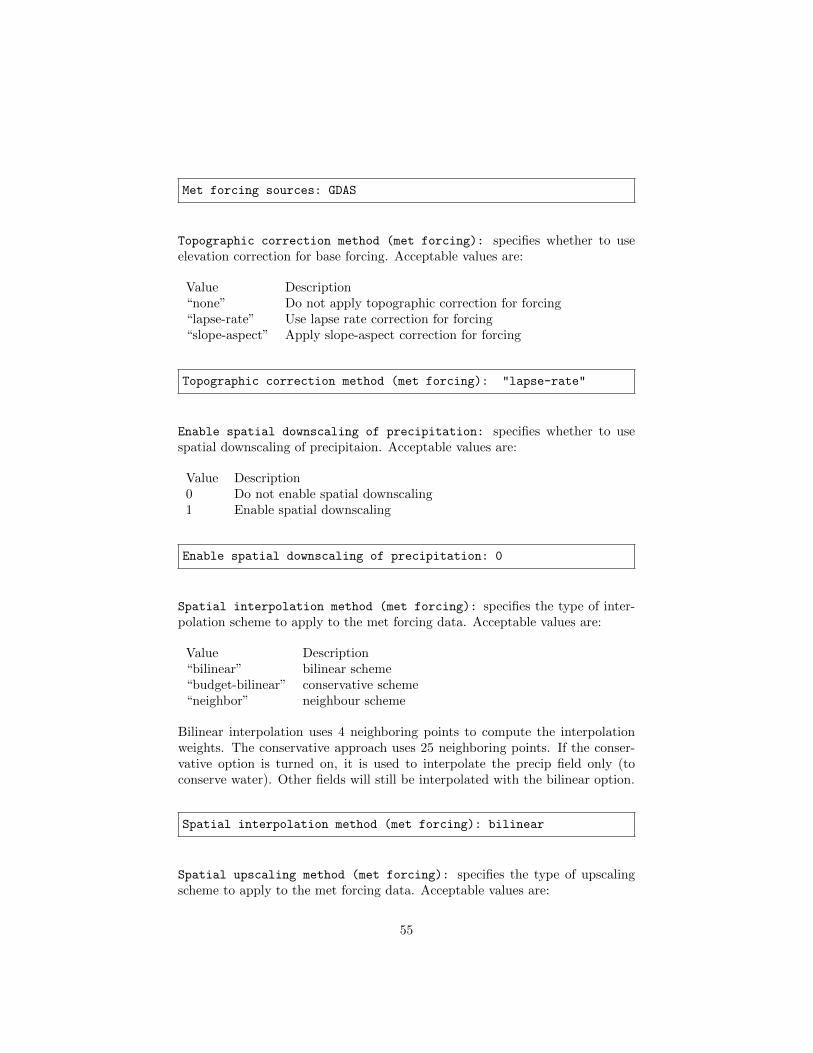
Met forcing sources: GDAS

Topographic correction method (met forcing): specifies whether to useelevation correction for base forcing. Acceptable values are:

Value Description“none” Do not apply topographic correction for forcing“lapse-rate” Use lapse rate correction for forcing“slope-aspect” Apply slope-aspect correction for forcing

Topographic correction method (met forcing): "lapse-rate"

Enable spatial downscaling of precipitation: specifies whether to usespatial downscaling of precipitaion. Acceptable values are:

Value Description0 Do not enable spatial downscaling1 Enable spatial downscaling

Enable spatial downscaling of precipitation: 0

Spatial interpolation method (met forcing): specifies the type of inter-polation scheme to apply to the met forcing data. Acceptable values are:

Value Description“bilinear” bilinear scheme“budget-bilinear” conservative scheme“neighbor” neighbour scheme

Bilinear interpolation uses 4 neighboring points to compute the interpolationweights. The conservative approach uses 25 neighboring points. If the conser-vative option is turned on, it is used to interpolate the precip field only (toconserve water). Other fields will still be interpolated with the bilinear option.

Spatial interpolation method (met forcing): bilinear

Spatial upscaling method (met forcing): specifies the type of upscalingscheme to apply to the met forcing data. Acceptable values are:

55

Value Description“average” averaging scheme

Please note that not all met forcing readers support upscaling of the met forcingdata.

Spatial upscaling method (met forcing): average

Temporal interpolation method (met forcing): specifies the type of tem-poral interpolation scheme to apply to the met forcing data. Acceptable valuesare:

Value Descriptionlinear linear schemetrilinear uber next scheme

The linear temporal interpolation method computes the temporal weights basedon two points. Ubernext computes weights based on three points. Currentlythe ubernext option is implemented only for the GSWP forcing.

Temporal interpolation method (met forcing): linear

9.2 Runtime options

Forcing variables list file: specifies the file containing the list of forcingvariables to be used. Please refer to the sample forcing variables.txt (Section 10)file for a complete specification description.

Forcing variables list file: ./input/forcing_variables.txt

Output methodology: specifies whether to write output as a 1-D array contain-ing only land points or as a 2-D array containing both land and water points.1-d tile space includes the subgrid tiles and ensembles. 1-d grid space includesa vectorized, land-only grid-averaged set of values. Acceptable values are:

Value Description“none” Do not write output“1d tilespace” Write output in a 1-D tile domain“2d gridspace” Write output in a 2-D grid domain“1d gridspace” Write output in a 1-D grid domain

56

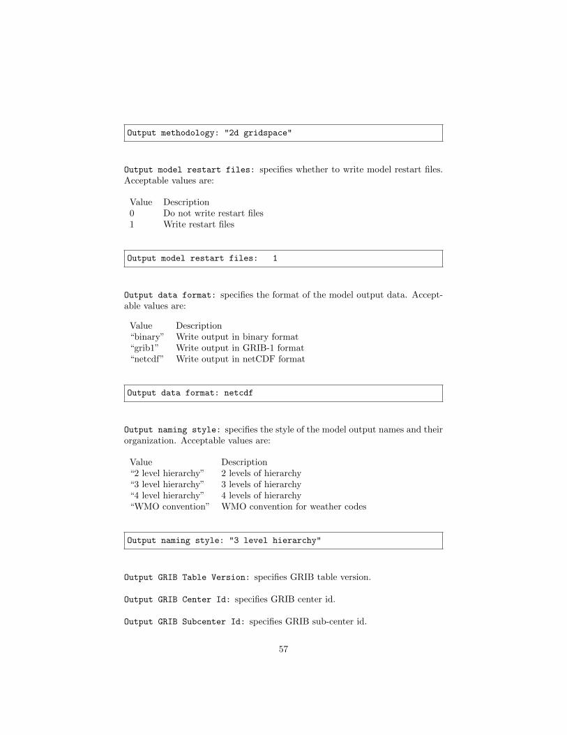
Output methodology: "2d gridspace"

Output model restart files: specifies whether to write model restart files.Acceptable values are:

Value Description0 Do not write restart files1 Write restart files

Output model restart files: 1

Output data format: specifies the format of the model output data. Accept-able values are:

Value Description“binary” Write output in binary format“grib1” Write output in GRIB-1 format“netcdf” Write output in netCDF format

Output data format: netcdf

Output naming style: specifies the style of the model output names and theirorganization. Acceptable values are:

Value Description“2 level hierarchy” 2 levels of hierarchy“3 level hierarchy” 3 levels of hierarchy“4 level hierarchy” 4 levels of hierarchy“WMO convention” WMO convention for weather codes

Output naming style: "3 level hierarchy"

Output GRIB Table Version: specifies GRIB table version.

Output GRIB Center Id: specifies GRIB center id.

Output GRIB Subcenter Id: specifies GRIB sub-center id.

57

Output GRIB Grid Id: specifies GRIB grid id.

Output GRIB Process Id: specifies GRIB process id.

Output GRIB Table Version: 130

Output GRIB Center Id: 173

Output GRIB Subcenter Id: 4

Output GRIB Grid Id: 11

Output GRIB Process Id: 1

Start mode: specifies if a restart mode is being used. Acceptable values are:

Value Descriptionrestart A restart mode is being usedcoldstart A cold start mode is being used, no restart file read

When the cold start option is specified, the program is initialized using theLSM-specific initial conditions (typically assumed uniform for all tiles). Whena restart mode is used, it is assumed that a corresponding restart file is provideddepending upon which LSM is used. The user also needs to make sure that theending time of the simulation is greater than model time when the restart filewas written.

Start mode: coldstart

The start time is specified in the following format:

Variable Value DescriptionStarting year: integer 2001 – present specifying starting yearStarting month: integer 1 – 12 specifying starting monthStarting day: integer 1 – 31 specifying starting dayStarting hour: integer 0 – 23 specifying starting hourStarting minute: integer 0 – 59 specifying starting minuteStarting second: integer 0 – 59 specifying starting second

Starting year: 2002

Starting month: 10

Starting day: 29

Starting hour: 1

Starting minute: 0

Starting second: 0

58

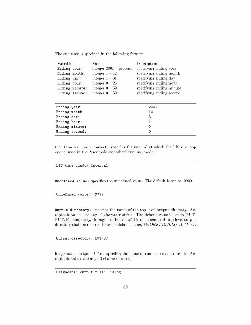
The end time is specified in the following format:

Variable Value DescriptionEnding year: integer 2001 – present specifying ending yearEnding month: integer 1 – 12 specifying ending monthEnding day: integer 1 – 31 specifying ending dayEnding hour: integer 0 – 23 specifying ending hourEnding minute: integer 0 – 59 specifying ending minuteEnding second: integer 0 – 59 specifying ending second

Ending year: 2002

Ending month: 10

Ending day: 31

Ending hour: 1

Ending minute: 0

Ending second: 0

LIS time window interval: specifies the interval at which the LIS run loopcycles, used in the “ensemble smoother” running mode.

LIS time window interval:

Undefined value: specifies the undefined value. The default is set to -9999.

Undefined value: -9999

Output directory: specifies the name of the top-level output directory. Ac-ceptable values are any 40 character string. The default value is set to OUT-PUT. For simplicity, throughout the rest of this document, this top-level outputdirectory shall be referred to by its default name, $WORKING/LIS/OUTPUT.

Output directory: OUTPUT

Diagnostic output file: specifies the name of run time diagnostic file. Ac-ceptable values are any 40 character string.

Diagnostic output file: lislog

59

Number of ensembles per tile: specifies the number of ensembles of tiles tobe used. The value should be greater than or equal to 1.

Number of ensembles per tile: 1

The following options are used for subgrid tiling based on vegetation

Maximum number of surface type tiles per grid: defines the maximumsurface type tiles per grid (this can be as many as the total number of vegetationtypes).

Maximum number of surface type tiles per grid: 1

Minimum cutoff percentage (surface type tiles): defines the smallest per-centage of a cell for which to create a tile. The percentage value is expressed asa fraction.

Minimum cutoff percentage (surface type tiles): 0.05

Maximum number of soil texture tiles per grid: defines the maximumsoil texture tiles per grid (this can be as many as the total number of soiltexture types).

Maximum number of soil texture tiles per grid: 1

Minimum cutoff percentage (soil texture tiles): defines the smallest per-centage of a cell for which to create a tile. The percentage value is expressed asa fraction.

Minimum cutoff percentage (soil texture tiles): 0.05

Maximum number of soil fraction tiles per grid: defines the maximumsoil fraction tiles per grid (this can be as many as the total number of soilfraction types).

60

Maximum number of soil fraction tiles per grid: 1

Minimum cutoff percentage (soil fraction tiles): defines the smallestpercentage of a cell for which to create a tile. The percentage value is expressedas a fraction.

Minimum cutoff percentage (soil fraction tiles): 0.05

Maximum number of elevation bands per grid: defines the maximum ele-vation bands per grid (this can be as many as the total number of elevationband types).

Maximum number of elevation bands per grid: 1

Minimum cutoff percentage (elevation bands): defines the smallest per-centage of a cell for which to create a tile. The percentage value is expressed asa fraction.

Minimum cutoff percentage (elevation bands): 0.05

Maximum number of slope bands per grid: defines the maximum slope bandsper grid (this can be as many as the total number of slope band types).

Maximum number of slope bands per grid: 1

Minimum cutoff percentage (slope bands): defines the smallest percent-age of a cell for which to create a tile. The percentage value is expressed as afraction.

Minimum cutoff percentage (slope bands): 0.05

Maximum number of aspect bands per grid: defines the maximum aspectbands per grid (this can be as many as the total number of aspect band types).

61

Maximum number of aspect bands per grid: 1

Minimum cutoff percentage (aspect bands): defines the smallest percent-age of a cell for which to create a tile. The percentage value is expressed as afraction.

Minimum cutoff percentage (aspect bands): 0.05

This section specifies the 2-d layout of the processors in a parallel processingenvironment. The user can specify the number of processors along the east-westdimension and north-south dimension using Number of processors along x:

and Number of processors along y:, respectively. Note that the layout ofprocessors should match the total number of processors used. For example,if 8 processors are used, the layout can be specified as 1x8, 2x4, 4x2, or 8x1.Further, this section also allows the specification of halos around the domainson each processor using Halo size along x: and Halo size along y:.

Number of processors along x: 2

Number of processors along y: 2

Halo size along x: 0

Halo size along y: 0

Routing model: specifies the routing model to run. Acceptable values are:

Value Descriptionnone do not use a routing model“NLDAS router” use the NLDAS router“HYMAP router” use the HYMAP router

Number of application models: specifies the number of application modelsto run.

Routing model: none

Radiative transfer model: none

Number of application models: 0

62

9.3 Data assimilation

This section specifies the choice of data assimilation options.

Number of data assimilation instances: specifies the number of data as-similation instances. Valid values are 0 (no assimilation) or higher.

Number of data assimilation instances: 0

Data assimilation algorithm: specifies the choice of data assimilation algo-rithms. Acceptable values are:

Value Description“none” None“Direct insertion” Direct Insertion“EnKF” GMAO EnKF data assimilation“EnKS” GRACE ensemble Kalman filter data assimilation

Data assimilation algorithm: none

Data assimilation set: specifies the “assimilation set”, which is the instancerelated to the assimilation of a particular observation. Acceptable values are:

Value Description“none” none“AMSR-E(NASA) soil moisture” AMSRE L3 soil moisture daily gridded data (HDF format)“AMSR-E(LPRM) soil moisture” AMSRE L3 soil moisture daily gridded data (HDF format)“ECV soil moisture” ECV soil moisture“Windsat” Windsat“ANSA SCF” ANSA SCF“PMW snow” PMW-based SWE or snow depth“MODIS SCF” MODIS SCF“GRACE TWS” GRACE TWS“SMOPS soil moisture” SMOPS soil moisture

Data assimilation set: none

Data assimilation exclude analysis increments: specifies whether theanalysis increments are to be skipped. This option is typically used along with

63

the dynamic bias estimation algorithm. The user can choose to apply only thebias increments or both the bias increments and analysis increments. Acceptablevalues are:

Value Description0 Apply analysis increments1 Do not apply analysis increments

Data assimilation exclude analysis increments: 0

Data assimilation output interval for diagnostics: specifies the out-put diagnostics interval.


Data assimilation output interval for diagnostics: 1da

Data assimilation number of observation types: specifies the number ofopervation species/types used in the assimilation.

Data assimilation number of observation types: 0

Data assimilation output ensemble members: specifies whether to outputthe ensemble members. Acceptable values are:

Value Description0 Do not output the ensemble members1 Output the ensemble members

Data assimilation output ensemble members: 0

Data assimilation output processed observations: specifies whether theprocessed, quality-controlled observations are to be written (Note that a cor-responding observation plugin routine needs to be implemented). Acceptablevalues are:

Value Description0 Do not output the processed observations1 Output the processed observations

64

Data assimilation output processed observations: 0

Data assimilation output innovations: specifies whether a binary outputof the normalized innovations is to be written. Acceptable values are:

Value Description0 Do not output the innovations1 Output the innovations

Data assimilation output innovations: 0

Data assimilation use a trained forward model: specifies whether to usea trained forward model. Acceptable values are:

Value Description0 Do not use a trained forward model1 Use a trained forward model

Data assimilation trained forward model output file: specifies the nameof the output file for the trained forward model. The training is done by LDT,and thus, this file is produced by LDT.

Data assimilation use a trained forward model: 0

Data assimilation trained forward model output file: none

Bias estimation

Bias estimation algorithm: specifies the dynamic bias estimation algorithmto use. Acceptable values are:

Value Description“none” No dynamic bias estimation“Adaptive bias correction” NASA GMAO dynamic bias estimation

Bias estimation algorithm: none

Bias estimation attributes file: ASCII file that specifies the attributes ofthe bias estimation. A sample file is shown below, which lists the variable name

65

first. This is followed by the nparam value (0-no bias correction, 1- constantbias correction without diurnal cycle, 3- diurnal sine/cosine bias correction, 5 -semi-diurnal sine/cosine bias correction, 2-“time of day” bias correction with 2separate bias estimates per day, 4 - “time of day” bias correction with 4 separateestimates per day, 8 - “time of day” bias correction with 8 separate bias estimatesper day), tconst (which describes the time scale relative to the temporal spacingof the observations), and trelax (which specifies temporal relaxation parameter,in seconds)

#nparam tconst trelaxSoil Temperature1.0 0.05 86400.0

Bias estimation attributes file:

Bias estimation restart output frequency: Specifies the frequency of biasrestart files.


Bias estimation restart output frequency: 1da

Bias estimation start mode: This option specifies whether the bias param-eters are to be read from a checkpoint file. Acceptable values are:

Value Descriptionnone Do not use a bias restart fileread Use a bias restart file

Bias estimation start mode: none

Bias estimation restart file: Specifies the restart file to be used for ini-tializing bias parameters

Bias estimation restart file: none

Perturbations start mode: specifies if the perturbations settings should beread from a restart file. Acceptable values are:

66

Value Descriptioncoldstart None (cold start)restart Use restart file

Perturbations start mode: coldstart

Apply perturbation bias correction: specifies whether to apply the Ryuet al. algorithm, (JHM 2009), to forcing and model states to avoid undesirablebiases resulting from perturbations. Acceptable values are:

Value Description0 Do not apply1 Apply

Apply perturbation bias correction:

Perturbations restart output interval: specifies the perturbations restartoutput writing interval.


Perturbations restart output interval: 1da

Perturbations restart filename: specifies the name of the restart file, whichis used to initialize perturbation settings if a cold start option is not employed.

Perturbations restart filename: none

Forcing perturbation algorithm: specifies the algorithm for perturbing theforcing variables. Acceptable values are:

Value Description“none” None“GMAO scheme” GMAO perturbation algorithm

Forcing perturbation algorithm: none

67

Forcing perturbation frequency: specifies the forcing perturbation inter-val.


Forcing perturbation frequency: 1hr

Forcing attributes file: ASCII file that specifies the attributes of the forc-ing (for perturbations) A sample file is shown below, which lists 3 forcing vari-ables. For each variable, the name of the variable is specified first, followed bythe min and max values in the next line. This is repeated for each additionalvariable.

#varmin varmaxIncident Shortwave Radiation Level 0010.0 1300.0Incident Longwave Radiation Level 001-50.0 800.0Rainfall Rate Level 0010.0 0.001

Forcing attributes file: none

Forcing perturbation attributes file: ASCII file that specifies the at-tributes of the forcing perturbations. A sample file is shown below, which lists3 forcing variables. There are three lines of specifications for each variable.The first line specifies the name of the variable. The second line specifies theperturbation type (0-additive, 1-multiplicative) and the perturbation type forstandard deviation (0-additive, 1-multiplicative). The third line specifies thefollowing values in that order: standard deviation of perturbations, coefficientof standard deviation (if perturbation type for standard deviation is 1),standardnormal max, whether to enable zero mean in perturbations, temporal correla-tion scale (in seconds), x and y -correlations and finally the cross correlationswith other variables.

#ptype std std max zeromean tcorr xcorr ycorr ccorrIncident Shortwave Radiation Level 0011 00.50 2.5 1 86400 0 0 1.0 -0.5 -0.8Incident Longwave Radiation Level 0010 150.0 0.2 2.5 1 86400 0 0 -0.5 1.0 0.5

68

Rainfall Rate Level 0011 00.50 2.5 1 86400 0 0 0.8 0.5 1.0

Forcing perturbation attributes file: none

State perturbation algorithm: specifies the algorithm for perturbing thestate prognostic variables. Acceptable values are:


State perturbation algorithm: none

State perturbation frequency: specifies the prognostic variable perturba-tion interval.


State perturbation frequency: 1hr

State attributes file: ASCII file that specifies the attributes of the prog-nostic variables. A sample file is shown below, which lists 2 model state vari-ables. For each variable, the name of the variable is specified first, followed bythe min and max values in the next line. This is repeated for each additionalvariable.

#name varmin varmaxSWE0.0 100.0Snowdepth0.0 100.0

State attributes file: none

State perturbation attributes file: ASCII file that specifies the attributesof the prognostic variable perturbations. A sample file is provided below, whichfollows the same format as that of the forcing perturbations attributes file:

69

#perttype std std max zeromean tcorr xcorr ycorr ccorrSWE1 00.01 2.5 1 10800 0 0 1.0 0.9Snowdepth1 00.02 2.5 1 10800 0 0 0.9 1.0

State perturbation attributes file: none

Observation perturbation algorithm: specifies the algorithm for perturb-ing the observations. Acceptable values are:


Observation perturbation algorithm: none

Observation perturbation frequency: specifies the observation perturba-tion interval.


Observation perturbation frequency: 1hr

Observation attributes file: ASCII file that specifies the attributes of theobservation variables. A sample file is provided below, which follows the sameformat as that of the forcing attributes file and state attributes file.

#error rate varmin varmaxANSA SWE10.0 0.01 500

Observation attributes file: none

Observation perturbation attributes file: ASCII file that specifies theattributes of the observation variable perturbations. A sample file is provided

70

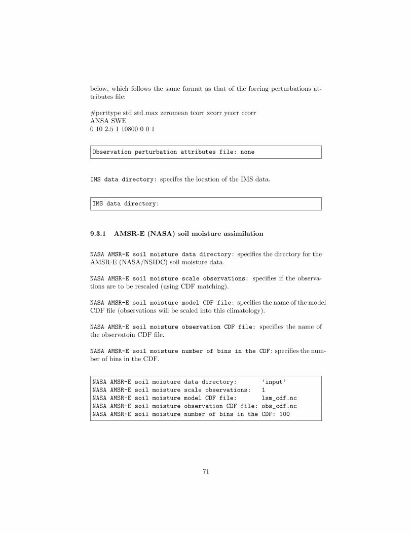
below, which follows the same format as that of the forcing perturbations at-tributes file:

#perttype std std max zeromean tcorr xcorr ycorr ccorrANSA SWE0 10 2.5 1 10800 0 0 1

Observation perturbation attributes file: none

IMS data directory: specifes the location of the IMS data.

IMS data directory:

9.3.1 AMSR-E (NASA) soil moisture assimilation

NASA AMSR-E soil moisture data directory: specifies the directory for theAMSR-E (NASA/NSIDC) soil moisture data.

NASA AMSR-E soil moisture scale observations: specifies if the observa-tions are to be rescaled (using CDF matching).

NASA AMSR-E soil moisture model CDF file: specifies the name of the modelCDF file (observations will be scaled into this climatology).

NASA AMSR-E soil moisture observation CDF file: specifies the name ofthe observatoin CDF file.

NASA AMSR-E soil moisture number of bins in the CDF: specifies the num-ber of bins in the CDF.

NASA AMSR-E soil moisture data directory: ’input’

NASA AMSR-E soil moisture scale observations: 1

NASA AMSR-E soil moisture model CDF file: lsm_cdf.nc

NASA AMSR-E soil moisture observation CDF file: obs_cdf.nc

NASA AMSR-E soil moisture number of bins in the CDF: 100

71

9.3.2 AMSR-E (LPRM) soil moisture assimilation

AMSR-E(LPRM) soil moisture data directory: specifies the directory forthe AMSR-E (LPRM) soil moisture data.

AMSR-E(LPRM) soil moisture use raw data: specifies if the the raw fields(in wetness units) or scaled fields (in volumetric units) are to be used.

AMSR-E(LPRM) scale observations: specifies if the observations are to berescaled (using CDF matching).

AMSR-E(LPRM) use scaled standard deviation model: specifies if the ob-servation error standard deviation is to be scaled using model and observationstandard deviation.

AMSR-E(LPRM) model CDF file: specifies the name of the model CDF file (ob-servations will be scaled into this climatology).

AMSR-E(LPRM) observation CDF file: specifies the name of the observatoinCDF file.

AMSR-E(LPRM) soil moisture number of bins in the CDF: specifies the num-ber of bins in the CDF.

AMSR-E(LPRM) soil moisture data directory: ’input’

AMSR-E(LPRM) soil moisture use raw data: 0

AMSR-E(LPRM) scale observations: 1

AMSR-E(LPRM) use scaled standard deviation model: 1

AMSR-E(LPRM) model CDF file: lsm_cdf.nc

AMSR-E(LPRM) observation CDF file: obs_cdf.nc

AMSR-E(LPRM) soil moisture number of bins in the CDF: 100

9.3.3 ECV soil moisture assimilation

ECV soil moisture data directory: specifies the directory for the ECV soilmoisture data.

ECV scale observations: specifies if the observations are to be rescaled (us-ing CDF matching).

ECV use scaled standard deviation model: specifies if the observation er-ror standard deviation is to be scaled using model and observation standard

72

deviation.

ECV model CDF file: specifies the name of the model CDF file (observationswill be scaled into this climatology).

ECV observation CDF file: specifies the name of the observatoin CDF file.

ECV soil moisture number of bins in the CDF: specifies the number of binsin the CDF.

ECV soil moisture data directory: ’input’

ECV scale observations: 1

ECV use scaled standard deviation model: 1

ECV model CDF file: lsm_cdf.nc

ECV observation CDF file: obs_cdf.nc

ECV soil moisture number of bins in the CDF: 100

9.3.4 WindSat soil moisture assimilation

WindSat soil moisture data directory: specifies the directory for the Wind-Sat soil moisture data.

WindSat scale observations: specifies if the observations are to be rescaled(using CDF matching).

WindSat model CDF file: specifies the name of the model CDF file (observa-tions will be scaled into this climatology).

WindSat observation CDF file: specifies the name of the observatoin CDFfile.

WindSat number of bins in the CDF: specifies the number of bins in theCDF.

WindSat soil moisture data directory: ’input’

WindSat scale observations: 1

WindSat model CDF file: lsm_cdf.nc

WindSat observation CDF file: obs_cdf.nc

WindSat number of bins in the CDF: 100

73

9.3.5 ANSA Snow Covered Fraction (SCF) Assimilation

ANSA SCF data directory: specifies the directory for the ANSA SCA data.

ANSA SCF lower left lat: specifies the lower left latitude of the ANSA do-main. (cylindrical latitude/longitude projection)

ANSA SCF lower left lon: specifies the lower left longitude of the ANSAdomain. (cylindrical latitude/longitude projection)

ANSA SCF upper right lat: specifies the upper right latitude of the ANSAdomain. (cylindrical latitude/longitude projection)

ANSA SCF upper right lon: specifies the upper right longitude of the ANSAdomain. (cylindrical latitude/longitude projection)

ANSA SCF resolution (dx): specifies the resolution of the of the ANSA do-main along the east-west direction.

ANSA SCF resolution (dy): specifies the resolution of the of the ANSA do-main along the north-south direction.

ANSA SCF local time for assimilation: specifies the local time for per-forming the ANSA SCF assimilation; LIS will find the closest time dependingon model timestep.

ANSA SCF field name: specifies the name of the SCF field to be assimilatedin the ANSA SCF data file.

ANSA SCF file name convention: specifies the name convention of the ANSASCF file; currently supported: *YYYYMMDD*, *YYYYDOY*.

ANSA SCF use triangular-shaped observation error: specifies whether touse a triangular-shaped observation error as follows (De Lannoy et al., 2012):std = std ∗ scf obs if scf obs <= 50; std = std ∗ (100 − scf obs) if scf obs >50; otherwise, std remains to be the same as read in from the observationperturbation attributes file.

ANSA SCF using EnKF with DI: specifies whether to used rule-based directinsertion approach to supplement EnKF when model predicts zero or full snowcover for all ensemble memebers. The entries after this are needed only if 1 isspecified here.

ANSA SCF direct insertion methodology: specifies which rule to use whenmodel predicts snow and observation says no snow. Acceptable values are:

74

Value Description“standard” use Rodell and Houser (2004)“customized” use Liu et al. (2013)

ANSA SCF amount of SWE (mm) to add to model: specifies how much swe toadd to model when observation sees snow while model predicts no snow.

ANSA SCF maximum SWE melt rate (mm/day): specifies the swe melt rate if“customized” is chosen for the direction insertion methodology.

ANSA SCF threshold of model SWE to be removed at once: specifies thethreshold of model SWE to be removed when observation says no snow.

ANSA SCF length of snowmelt period in days: specifies the length of thetypical snowmelt period in the region.

ANSA SCF threshold of observed SCF for snow presence: specifies the thresh-old of observed SCF for indicating snow presence.

ANSA SCF threshold of observed SCF for snow non-presence: specifies thethreshold of obsered SCF for indicating snow non-presence.

ANSA SCF threshold of model SWE(mm) for snow non-presence: specifiesthe threshold of model SWE for indicating snow absence.

ANSA SCF threshold of observed SCF for non-full snow cover: specifiesthe threshold of observed SCF which indicates non-full snow cover.

ANSA SCF data directory: ./ANSA_SCF_UCO

ANSA SCF lower left lat: 35.025

ANSA SCF lower left lon: -112.475

ANSA SCF upper right lat: 43.975

ANSA SCF upper right lon: -105.525

ANSA SCF resolution (dx): 0.05

ANSA SCF resolution (dy): 0.05

ANSA SCF local time for assimilation: 10.0

ANSA SCF field name: "/ansa_interpsnow"

ANSA SCF file name convention: "ansa_all_YYYYMMDD.h5"

ANSA SCF use triangular-shaped observation error: 1

ANSA SCF using EnKF with DI: 1

ANSA SCF direct insertion methodology: "customized"

ANSA SCF amount of SWE (mm) to add to model: 10

ANSA SCF maximum SWE melt rate (mm/day): 50

ANSA SCF threshold of model SWE to be removed at once: 20

ANSA SCF length of snowmelt period in days: 15

75

ANSA SCF threshold of observed SCF for snow presence: 0.4

ANSA SCF threshold of observed SCF for snow non-presence: 0.1

ANSA SCF threshold of model SWE(mm) for snow non-presence: 5

ANSA SCF threshold of observed SCF for non-full snow cover: 0.7

9.3.6 MODIS snow cover fraction assimilation

MODIS SCF data directory: specifies the directory for the MODIS snow coverfraction data.

MODIS SCF use gap filled product: specifies whether the gap-filled productis to be used (1-use, 0-do not use).

MODIS SCF cloud threshold: Cloud cover threshold to be used for screeningobservations (in percentage).

MODIS SCF cloud persistence threshold: Cloud cover persistence thresh-old to be used for screening observations (in days).

MODIS SCF data directory: ./MODIS

MODIS SCF use gap filled product: 1

MODIS SCF cloud threshold: 90

MODIS SCF cloud persistence threshold: 3

9.3.7 PMW snow depth or SWE assimilation

PMW snow data directory: specifies the directory for the PMW SWE or snowdepth data.

PMW snow data file format (HDF4, HDF-EOS, HDF5): specifies the file for-mat of the PMW snow data. Currently, three options are supported: HDF4,HDF-EOS, and HDF5

PMW snow data coordindate system (EASE, LATLON): specifies the coordi-nate system of the PMW snow data. Currently two options are supported:EASE and LATLON.

PMW snow data variable (SWE, snow depth): specifies which variable to as-similate: SWE or snow depth

76

PMW snow data unit (m, cm, mm, inch): specifies the unit of the snow data;currently only units of m, cm, mm, inch are supported

PMW snow data use flag (1=yes, 0=no): specifies whether to use the dataflags that come along with the PMW snow data in the same file

PMW snow data flag - number of invalid values: specifies the number ofinvalid values in the flag field of the PMW snow data

PMW snow data flag - invalid values: specifies the invalid values of theflag field of the PMW snow data

PMW snow data - number of additional invalid values: specifies the num-ber of additional invalid values in the actual data field of the PMW snow data

PMW snow data - additional invalid values: specifies the invalid valuesof the actual data field of the PMW snow data

PMW snow data - apply min/max mask: specifies whether to use min/maxdata values for quality control of the PMW snow data

PMW snow data minimum valid value: specifies the minimum valid value ofthe PMW snow data

PMW snow data maximum valid value: specifies the maximum valid value ofthe PMW snow data

PMW snow data scale factor: specifies the scale factor of the PMW snowdata

PMW snow data file name convention: specifies the file name conventionof the PMW snow data; currently only the following two formats are sup-ported: *YYYYMMDD* and *YYYYDOY* note that the PMW snow readerassumes that the data files are stored in corresponding year directory as follows:datadir/YYYY/*YYYMMDD*

PMW snow data assimilation local time: specifies the local time in hoursto apply the assimilation (usually corresponding to the overpass time)

PMW snow data - apply mask with GVF (1=yes, 0=no): specifies whetherto use greenness vegetation fraction as mask for assimilation; 1 is suggestedunless confidence is high with the PMW snow data (e.g., those that are biascorrected against station data) in dense vegetation area. If “1” is chosen, LISwill not assimilate PMW snow data in those areas with gvf >0.7.

PMW snow data - apply mask with landcover type (1=yes, 0=no): spec-

77

ifies whether to use landcover type as mask for assimilation. If “1” is chosen,LIS will not assimilate PMW snow data in areas with forest land cover.

PMW snow data - apply mask with LSM temperature (1=yes, 0=no): spec-ifies whether to use model-based temperatures as mask for assimilation. if “1”is chosen, LIS will not assimilate PMW snow data in areas with a skin temper-ature or surface soil temperature higher than 5 degree C according to the LSM.This mask should be used with care if the LSM temperatures are known to bebiased.

The following 8 configuration lines are for HDF5+LANTON datasets only

PMW snow data lower left lat: specifies the lower left latitude of the dataset.

PMW snow data lower left lon: specifies the lower left longitude of the dataset.

PMW snow data upper right lat: specifies the upper right latitude of thedataset.

PMW snow data upper right lon: specifies the upper right longitude of thedataset.

PMW snow data resolution (dx): specifies horizotal resolution dx of the dataset.

PMW snow data resolution (dy): specifies vertical resolution dy of the dataset.

PMW (HDF5) snow data field name: specifies the name of the snow data fieldin the dataset for assimilation.

PMW (HDF5) snow data flag field name: specifies the name of the snowdata flag field to use as a mask for assimilation; this must be specified if thePMW snow data use flag (1=yes, 0=no): option is set to 1.

The following 4 configuration lines are for HDF4+EASE datasets only

PMW (HDF4) snow data NL SDS index (-1, 0, 1, 2, ...): specifies the in-dex of the SDS of the NL grid in the PMW snow data; valid index starts from0; use -1 if no SDS for the NL grid is to be assimilated.

PMW (HDF4) snow data SL SDS index (-1, 0, 1, 2, ...): specifies the in-dex of the SDS of the SL grid in the PMW snow data; valid index starts from0; use -1 if no SDS for the NL grid is to be assimilated.

PMW (HDF4) snow data flag NL SDS index (-1, 0, 1, 2, ...): specifiesthe index of the flag SDS of the NL grid in the PMW snow data; this must bespecified if the PMW snow data use flag (1=yes, 0=no): option is set to 1.

78

PMW (HDF4) snow data flag SL SDS index (-1, 0, 1, 2, ...): specifiesthe index of the flag SDS of the SL grid in the PMW snow data; this must bespecified if the PMW snow data use flag (1=yes, 0=no): option is set to 1.

The following 6 configuration lines are for HDF-EOS+EASE datasets only

PMW (HDF-EOS) NL grid name: specifies the name of the NL grid.

PMW (HDF-EOS) SL grid name: specifies the name of the SL grid.

PMW (HDF-EOS) NL SDS name: specifies the name of the SDS in the NL grid.

PMW (HDF-EOS) SL SDS name: specifies the name of the SDS in the SL grid.

PMW (HDF-EOS) NL snow data flag SDS name: specifies the name of the dataflag SDS in the NL grid; this must be specified if the PMW snow data use flag

(1=yes, 0=no): option is set to 1.

PMW (HDF-EOS) SL snow data flag SDS name: specifies the name of the dataflag SDS in the SL grid; this must be specified if the PMW snow data use flag

(1=yes, 0=no): option is set to 1.

# all datasets

PMW snow data directory: "./input/ANSA_OI"

PMW snow data file format (HDF4, HDF-EOS, HDF5): "HDF5"

PMW snow data coordindate system (EASE, LATLON): "LATLON"

PMW snow data variable (SWE, snow depth): "snow depth"

PMW snow data unit (m, cm, mm, inch): "mm"

PMW snow data use flag (1=yes, 0=no): 1

PMW snow data flag - number of invalid values: 2

PMW snow data flag - invalid values: -1 0

PMW snow data - number of additional invalid values: 0

PMW snow data - additional invalid values: 494 496 504 596 508 510

PMW snow data - apply min/max mask: 1

PMW snow data minimum valid value: 0

PMW snow data maximum valid value: 5000

PMW snow data scale factor: 1.0

PMW snow data file name convention: "ansa_all_YYYYMMDD.h5"

PMW snow data assimilation local time: 2.0

PMW snow data - apply mask with GVF (1=yes, 0=no): 0

PMW snow data - apply mask with landcover type (1=yes, 0=no): 0

PMW snow data - apply mask with LSM temperature (1=yes, 0=no): 0

# HDF5 & LATLON datasets only

PMW snow data lower left lat: 50.025

79

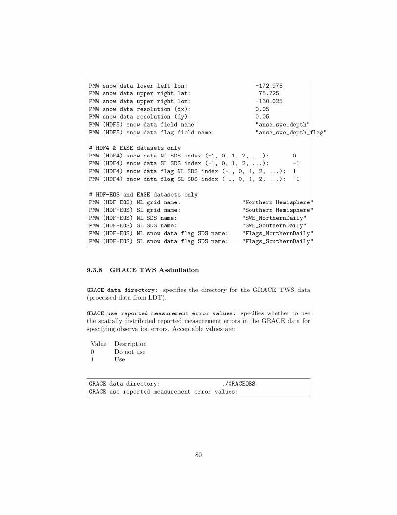
PMW snow data lower left lon: -172.975

PMW snow data upper right lat: 75.725

PMW snow data upper right lon: -130.025

PMW snow data resolution (dx): 0.05

PMW snow data resolution (dy): 0.05

PMW (HDF5) snow data field name: "ansa_swe_depth"

PMW (HDF5) snow data flag field name: "ansa_swe_depth_flag"

# HDF4 & EASE datasets only

PMW (HDF4) snow data NL SDS index (-1, 0, 1, 2, ...): 0

PMW (HDF4) snow data SL SDS index (-1, 0, 1, 2, ...): -1

PMW (HDF4) snow data flag NL SDS index (-1, 0, 1, 2, ...): 1

PMW (HDF4) snow data flag SL SDS index (-1, 0, 1, 2, ...): -1

# HDF-EOS and EASE datasets only

PMW (HDF-EOS) NL grid name: "Northern Hemisphere"

PMW (HDF-EOS) SL grid name: "Southern Hemisphere"

PMW (HDF-EOS) NL SDS name: "SWE_NorthernDaily"

PMW (HDF-EOS) SL SDS name: "SWE_SouthernDaily"

PMW (HDF-EOS) NL snow data flag SDS name: "Flags_NorthernDaily"

PMW (HDF-EOS) SL snow data flag SDS name: "Flags_SouthernDaily"

9.3.8 GRACE TWS Assimilation

GRACE data directory: specifies the directory for the GRACE TWS data(processed data from LDT).

GRACE use reported measurement error values: specifies whether to usethe spatially distributed reported measurement errors in the GRACE data forspecifying observation errors. Acceptable values are:

Value Description0 Do not use1 Use

GRACE data directory: ./GRACEOBS

GRACE use reported measurement error values:

80

9.3.9 SMOPS soil moisture assimilation

SMOPS soil moisture data directory: specifies the directory for the SMOPSsoil moisture data.

SMOPS soil moisture use ASCAT data: specifies if the ASCAT data layer isto be used.

SMOPS use scaled standard deviation model: specifies if the observationerror standard deviation is to be scaled using model and observation standarddeviation.

SMOPS model CDF file: specifies the name of the model CDF file (observationswill be scaled into this climatology).

SMOPS observation CDF file: specifies the name of the observation CDF file.

SMOPS soil moisture number of bins in the CDF: specifies the number ofbins in the CDF.

SMOPS use realtime data: specifies whether to use the 6 hour data feed in-stead of the daily data feed. Acceptable values are:

Value Description0 Use daily data feed1 Use 6 hour data feed

SMOPS soil moisture use scaled standard deviation model: specifies whetherto use scaled standard deviation. This generates and uses spatially distributedobservation errors by scaling the specified observation error standard deviationby a factor of the model standard deviation to the observation standard devia-tion. (e 7→ e×mσ/oσ)

SMOPS naming convention: specifies the naming convention of the SMOPSsoil moisture data. Used when reading the 6-hour data feed. Acceptable valuesare:

Value Description“LIS” YYYY/NPR SMOPS CMAP DYYYYMMDDHH.gr2“other” smops dYYYYMMDD sHH0000 cness.gr2

SMOPS soil moisture data directory: ’input’

SMOPS soil moisture use ASCAT data: 1

SMOPS use scaled standard deviation model: 1

SMOPS model CDF file: lsm_cdf.nc

81

SMOPS observation CDF file: obs_cdf.nc

SMOPS soil moisture number of bins in the CDF: 100

SMOPS use realtime data:

SMOPS soil moisture use scaled standard deviation model:

SMOPS naming convention: LIS

9.4 Radiative Transfer/Forward Models

This section specifies the choice of radiative transfer or forward modeling tools.

Radiative transfer model: specifies which RTM is to be used. Acceptablevalues are:

Value DescriptionCRTM2EM CRTM2EMCMEM CMEM

RTM invocation frequency: specifies the invocation frequency of the chosenRTM.


RTM history output frequency: specifies the history output frequency of theRTM.


Radiative transfer model: CRTM2EM

RTM invocation frequency: 1hr

RTM history output frequency: 3hr

9.4.1 CRTM2EM

This section specifies the specifications to enable a CRTM2EM instance.

CRTM number of sensors: specifies the number of sensors to be used.

CRTM number of layers: specifies the number of atmospheric layers.

CRTM number of absorbers: specifies the number of absorbers.

82

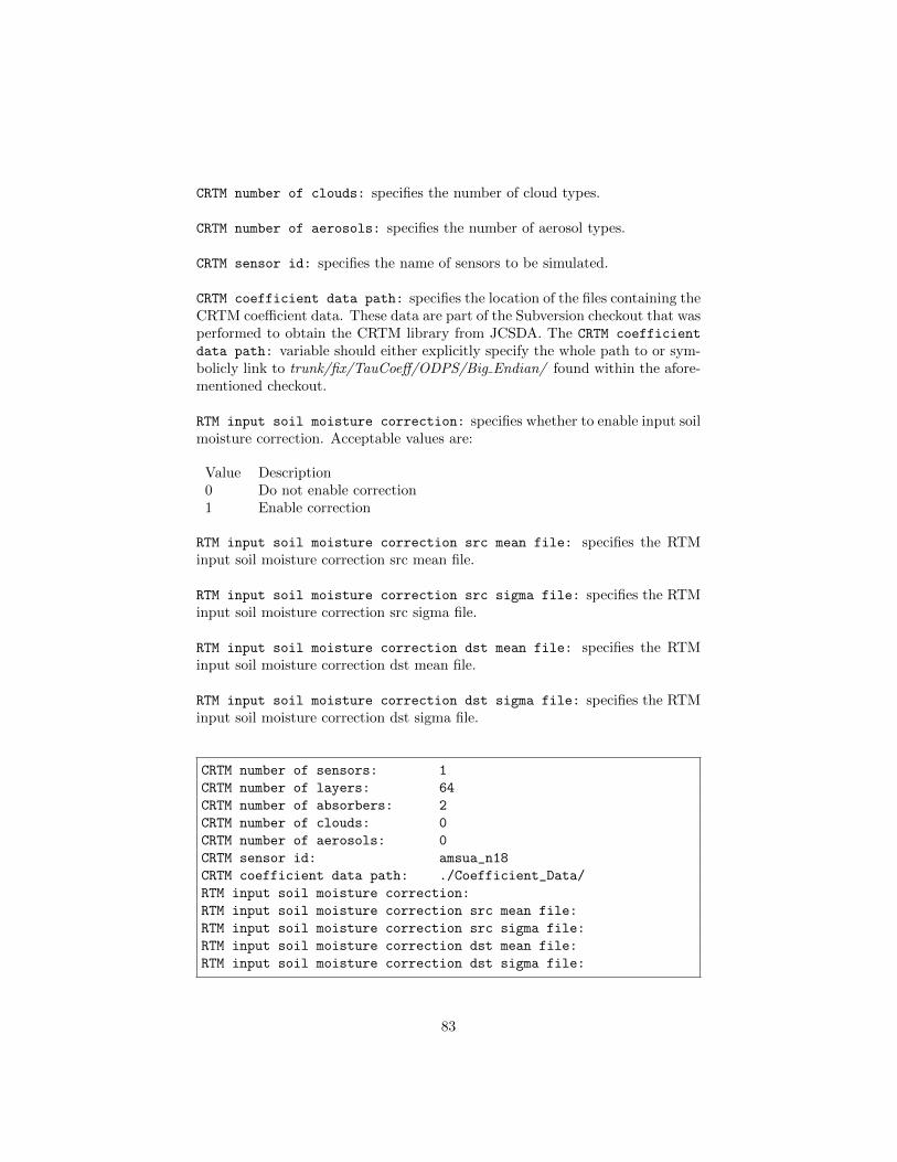
CRTM number of clouds: specifies the number of cloud types.

CRTM number of aerosols: specifies the number of aerosol types.

CRTM sensor id: specifies the name of sensors to be simulated.

CRTM coefficient data path: specifies the location of the files containing theCRTM coefficient data. These data are part of the Subversion checkout that wasperformed to obtain the CRTM library from JCSDA. The CRTM coefficient

data path: variable should either explicitly specify the whole path to or sym-bolicly link to trunk/fix/TauCoeff/ODPS/Big Endian/ found within the afore-mentioned checkout.

RTM input soil moisture correction: specifies whether to enable input soilmoisture correction. Acceptable values are:

Value Description0 Do not enable correction1 Enable correction

RTM input soil moisture correction src mean file: specifies the RTMinput soil moisture correction src mean file.

RTM input soil moisture correction src sigma file: specifies the RTMinput soil moisture correction src sigma file.

RTM input soil moisture correction dst mean file: specifies the RTMinput soil moisture correction dst mean file.

RTM input soil moisture correction dst sigma file: specifies the RTMinput soil moisture correction dst sigma file.

CRTM number of sensors: 1

CRTM number of layers: 64

CRTM number of absorbers: 2

CRTM number of clouds: 0

CRTM number of aerosols: 0

CRTM sensor id: amsua_n18

CRTM coefficient data path: ./Coefficient_Data/

RTM input soil moisture correction:

RTM input soil moisture correction src mean file:

RTM input soil moisture correction src sigma file:

RTM input soil moisture correction dst mean file:

RTM input soil moisture correction dst sigma file:

83

9.4.2 CMEM3

This section specifies the specifications to enable a CMEM3 instance. For moreinformation regarding CMEM3, please seehttp://www.ecmwf.int/research/data assimilation/land surface/cmem/cmem index.html.

CMEM3 sensor id: specifies the name of sensors to be simulated.

CMEM3 number of frequencies: specifies the number of frequencies.

CMEM3 frequencies file: specifies the file containing the CMEM3 frequenciesdata. This is an ASCII file containing two columns of data. The first columnspecifies frequency in GHz; the second column specifies the incidence angle. Asample file for AMSR-E:

6.925 55.010.65 55.018.7 55.023.8 55.036.5 55.089.0 55.0

RTM input soil moisture correction: specifies whether to enable input soilmoisture correction. Acceptable values are:

Value Description0 Do not enable correction1 Enable correction

RTM input soil moisture correction src mean file: specifies the RTMinput soil moisture correction src mean file.

RTM input soil moisture correction src sigma file: specifies the RTMinput soil moisture correction src sigma file.

RTM input soil moisture correction dst mean file: specifies the RTMinput soil moisture correction dst mean file.

RTM input soil moisture correction dst sigma file: specifies the RTMinput soil moisture correction dst sigma file.

CMEM3 sensor id: amsre

CMEM3 number of frequencies: ./amsre-freqs.tx

CMEM3 frequencies file:

RTM input soil moisture correction:

84

http://www.ecmwf.int/research/data_assimilation/land_surface/cmem/cmem_index.html

RTM input soil moisture correction src mean file:

RTM input soil moisture correction src sigma file:

RTM input soil moisture correction dst mean file:

RTM input soil moisture correction dst sigma file:

9.5 Optimization and Uncertainty Estimation

This section specifies options for carrying out parameter estimation and uncer-tainty estimation.

Optimization/Uncertainty Estimation Algorithm: Specifies which algorithmis to be used for optimization. Acceptable values are:

Value Description“none” no optimization“Genetic algorithm” Genetic Algorithm“Monte carlo sampling” MCSIM Algorithm“Differential evolution markov chain z” DEMCz Algorithm

Optimization/Uncertainty Estimation Set: specifies the calibration dataset, which represents the observation source used in the particular parameterestimation instance. Acceptable values are:

Value Description“No obs” no observations“AMSRE SR” AMSR-E (Colorado State Univ.)“AMSR-E(LPRM) pe soil moisture” AMSR-E LPRM soil moisture

Objective Function Method: specifies the objective function method. Ac-ceptable values are:

Value Description“Least squares” Least squares“Likelihood” Maximum likelihood“Probability” Maximize probability

Write PE Observations: specifies whether to output processed observationsfor parameter estimation Acceptable values are:

Value Description0 Do not write pe observations1 Write pe observations

85

Number of model types subject to parameter estimation: specifies thenumber of model classes used in a parameter estimation instance. E.g.: if LSMand RTM parameters are simultaneously being calibrated then this option willbe 2.

Model types subject to parameter estimation: specifies the names of themodel types to be used in the parameter estimation instance. E.g.: LSM RTM

Number of model types with observation predictors for parameter estimation:

specifies the number of model types (e.g., LSM, RTM) that will be generatingpredictions of observations for comparison against real observations when con-ducting parameter or uncertainty estimation. Acceptable values are either 1 or2.

Model types with observation predictors for parameter estimation: spec-ifies the list of model types (e.g., LSM, RTM) that will be generating predictionsof observations for comparison against real observations when conducting pa-rameter or uncertainty estimation. Acceptable values are a combination of LSMand/or RTM.

Initialize decision space with default values: specifies whether to usedefaults instead of sampled values at the beginning of optimization. Acceptablevalues are:

Value Description0 Use defaults1 Use sampled values

(Yes, this is backwards from what the label suggests.)

Calibration period start year: specifies the starting year of the calibrationperiod.

Calibration period start month: specifies the starting month of the cali-bration period.

Calibration period start day: specifies the starting day of the calibrationperiod.

Calibration period start hour: specifies the starting hour of the calibra-tion period.

Calibration period start minutes: specifies the starting minutes of thecalibration period.

Calibration period start seconds: specifies the starting seconds of the cal-ibration period.

86

9.5.1 Least squares

This section provides specifications of the LS objective function instance

Least Squares objective function weights file: specifies the file con-taining the weights to be applied to each objective function

Least Squares objective function mode: specifies which least squares ag-gregation to use. Acceptable values are:

Value Description1 distributed (ie, optimized for each cell independently)

Least Squares objective function minimum number of obs: for grid cellswith fewer obs than specified, least squares parameter estimation will not beconducted so as to avoid ’overfitting’ model to the data.

9.5.2 Probability

This section provides specifications of the Probability objective function in-stance.

Prior distribution attributes file: specifies the file containing the priorprobability distribution over the parameters

9.5.3 Likelihood

This section provides specifications of the Likelihood objective function instance.There are no additional specifications needed. Unlike the Probability objectivefunction, Likelihood does not factor in prior probability.

9.5.4 Genetic Algorithm

This section provides specifications of the genetic algorithm instance

GA restart file: specifies the name of the GA restart file.

GA number of generations: specifies the number of generations of GA.

GA number of children per parent: specifies how many offsprings are pro-

87

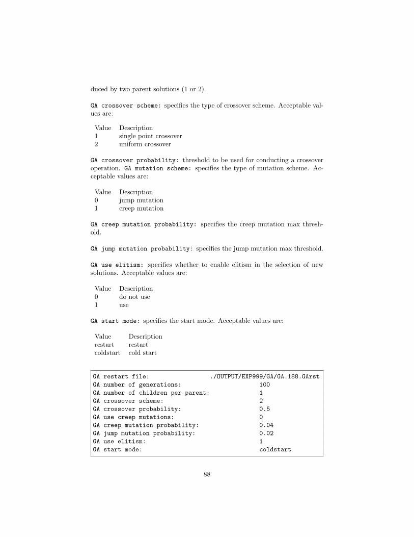
duced by two parent solutions (1 or 2).

GA crossover scheme: specifies the type of crossover scheme. Acceptable val-ues are:

Value Description1 single point crossover2 uniform crossover

GA crossover probability: threshold to be used for conducting a crossoveroperation. GA mutation scheme: specifies the type of mutation scheme. Ac-ceptable values are:

Value Description0 jump mutation1 creep mutation

GA creep mutation probability: specifies the creep mutation max thresh-old.

GA jump mutation probability: specifies the jump mutation max threshold.

GA use elitism: specifies whether to enable elitism in the selection of newsolutions. Acceptable values are:

Value Description0 do not use1 use

GA start mode: specifies the start mode. Acceptable values are:

Value Descriptionrestart restartcoldstart cold start

GA restart file: ./OUTPUT/EXP999/GA/GA.188.GArst

GA number of generations: 100

GA number of children per parent: 1

GA crossover scheme: 2

GA crossover probability: 0.5

GA use creep mutations: 0

GA creep mutation probability: 0.04

GA jump mutation probability: 0.02

GA use elitism: 1

GA start mode: coldstart

88

9.5.5 Differential Evolution Markov Chain (DEMCz) algorithm

This section provides specifications of the DEMCz algorithm instance. DEMCzis an instance of Bayesian analysis (Reference: Gelman et al. (1995)) conductedvia Markov chain Monte Carlo (MCMC) (Reference: Brooks et al. (2011)).MCMC enables generation of parameter ensembles for subsequent LIS ensem-ble runs, where the ensembles reflect user-specified probability distributions asupdated with observational datasets. Reference for DEMCz: ter Braak (2006),and ter Braak and Vrugt (2008). DEMCz implements DEMC with the ’samplingfrom the past’ of ter Braak and Vrugt (2008)

DEMCz restart file: specifies the name of the DEMCz restart file.

DEMCz number of iterations: specifies the number of iterations of DEMCz.

DEMCz GA restart file: specifies the GA solution that serves as the DEMCzalgorithm starting point

DEMCz perturbation factor: Applied uniformly to all parameters. The prod-uct of this term and the width of the parameter range (ie, max-min) determinesthe random-walk-like term (’b’) in the DEMCz algorithm

DEMCz mode hopping frequency: At this frequency (f), full jumps betweenseparated regions of high probability may occur (so as to better balance ex-ploration of each region) through the setting of a DEMCz control parameter(gamma=1); at frequency 1-f, the settings are optimized for exploration of thelocal region of high probability (gamma=2.38)

DEMCz start mode: specifies the start mode. Acceptable values are:

Value Descriptionrestart restartcoldstart cold start

DEMCz restart file: ./OUTPUT/DEMCz/DEMCz.188.DEMCzrst

DEMCz number of iterations: 100

DEMCz start mode: coldstart

DEMCz GA restart file: ./OUTPUT/GA/GA.188.GArst

DEMCz perturbation factor: 0.001

DEMCz mode hopping frequency: 0.10

89

9.5.6 Monte Carlo simulation

This section provides specifications of the MCSIM algorithm instance. MC-SIM randomly samples from user-specified probability distributions to generateparmeter ensembles for subsequent use in LIS ensemble runs. Unlike MCMCalgorithms (e.g., DEMCz), the probability distributions being sampled are thosegiven by the user, and not as updated with observational datasets. Algorithmreference: Morgan and Henrion (1990).

MCSIM number of iterations: specifies the number of iterations of MCSIM.This typically will be set to 1. Only set to values higher than 1 to accumulatemore samples than can be achieved in a single LIS ensemble run.

MCSIM start mode: specifies the start mode. The restart option, as just noted,would only be needed if the number of samples that can be achieved in a singleLIS ensemble run is limiting.

Acceptable values are:Value Descriptionrestart restartcoldstart cold start

MCSIM restart file: specifies the name of the MCSIM restart file.

MCSIM number of iterations: 1

MCSIM start mode: coldstart

MCSIM restart file: none

9.5.7 Observations for Parameter Estimation

This section of the config file includes the observation specifications for paramterestimation

9.5.8 AMSRE SR Emissivity

AMSRE SR data directory: specifies the location of the AMSR-E emissivityretrievals data.

AMSRE SR Emissivity observations attributes file: specifies the loca-tion of the observation attributes file.

90

AMSRE SR number of observations threshold: specifies how many observa-tions must be behind emissivity average for cell

AMSRE_SR Emissivity Obs data directory: ’./obs/’

AMSRE_SR Emissivity observations attributes file: ’./AMSRE_SR_attribs.txt’

AMSRE_SR number of observations threshold: 5

9.5.9 AMSR-E (LPRM) pe soil moisture

LPRM AMSRE soil moisture data directory: specifies the location of theAMSR-E LPRM soil moisture data.

LPRM AMSRE soil moisture observations attributes file: specifies thelocation of the observation attributes file.

LPRM AMSRE soil moisture data directory: ’./LPRM.v6’

LPRM AMSRE soil moisture observations attributes file: ’./LPRM_attribs.txt’

9.5.10 No obs

This PE observation option is used when conducting MCSIM as MCSIM doesnot factor in observational datasets in the sampling of parameter ensembles.There are no configuration options.

9.6 Parameters

LIS domain and parameter data file: specifies the primary input file thatcontains LIS parameter data.

LIS 7 includes a pre-processing system called the Land Data Toolkit (LDT). Itreads the raw parameter data and processes them to the LIS running domain.The LIS domain and parameter data file: is the result of the LDT pre-processing. Please read the “Land Data Toolkit (LDT) User’s Guide” for moreinformation.

LIS domain and parameter data file: ./lis_input.d01.nc

91

9.6.1 Parameter options

Landmask data source: specifies the usage of landmask data in the run. Ac-ceptable values are:

Value Descriptionnone Do not landmaskLDT Read landmask from the LDT-generated LIS domain and parameter data file:

Landcover data source: specifies the usage of landcover data in the run.Acceptable values are:

Value DescriptionLDT Read landcover data from the LDT-generated LIS domain and parameter data file:

Landmask data source: LDT

Landcover data source: LDT

Soil texture data source: specifies the usage of soil texture data in the run.Acceptable values are:

Value Descriptionnone Do not read soil textureLDT Read soil texture data from the LDT-generated LIS domain and parameter data file:

Soil texture data source: LDT

Soil fraction data source: specifies the usage of soil fraction parametersin the run. Acceptable values are:

Value Descriptionnone Do not read soil fractionsLDT Read soil fractions data from the LDT-generated LIS domain and parameter data file:

Soil fraction data source: none

Soil color data source: specifies the usage of soil color data in the run.Acceptable values are:

92

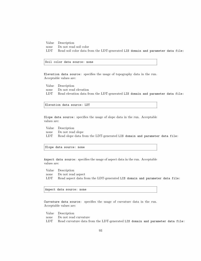
Value Descriptionnone Do not read soil colorLDT Read soil color data from the LDT-generated LIS domain and parameter data file:

Soil color data source: none

Elevation data source: specifies the usage of topography data in the run.Acceptable values are:

Value Descriptionnone Do not read elevationLDT Read elevation data from the LDT-generated LIS domain and parameter data file:

Elevation data source: LDT

Slope data source: specifies the usage of slope data in the run. Acceptablevalues are:

Value Descriptionnone Do not read slopeLDT Read slope data from the LDT-generated LIS domain and parameter data file:

Slope data source: none

Aspect data source: specifies the usage of aspect data in the run. Acceptablevalues are:

Value Descriptionnone Do not read aspectLDT Read aspect data from the LDT-generated LIS domain and parameter data file:

Aspect data source: none

Curvature data source: specifies the usage of curvature data in the run.Acceptable values are:

Value Descriptionnone Do not read curvatureLDT Read curvature data from the LDT-generated LIS domain and parameter data file:

93

Curvature data source: none

LAI data source: specifies the usage of LAI data in the run. Acceptablevalues are:

Value Descriptionnone Do not read LAILDT Read LAI data from the LDT-generated LIS domain and parameter data file:

“MODIS real-time” Read MODIS real-time LAI

LAI data source: none

SAI data source: specifies the usage of LAI data in the run. Acceptablevalues are:

Value Descriptionnone Do not read SAILDT Read SAI data from the LDT-generated LIS domain and parameter data file:

“MODIS real-time” Read MODIS real-time SAI

SAI data source: none

Albedo data source: specifies the usage of albedo data in the run. Acceptablevalues are:

Value Descriptionnone Do not read albedoLDT Read albedo data from the LDT-generated LIS domain and parameter data file:

Albedo data source: LDT

Max snow albedo data source: specifies the usage of the maximum snowalbedo in the run. Acceptable values are:

Value Descriptionnone Do not read max snow albedofixed Use fixed max snow albedo from the “lis.config” file.

This option is only available to the Noah-3.x LSMs.LDT Read max snow albedo data from the LDT-generated LIS domain and parameter data file:

94

Max snow albedo data source: LDT

Greenness data source: specifies the usage of greenness fraction data in therun. Acceptable values are:

Value Descriptionnone Do not read greenness fractionLDT Read greenness data from the LDT-generated LIS domain and parameter data file:

“NESDIS weekly” Read NESDIS weekly greenness fraction“SPORT” Read SPORT greenness fractionVIIRS Read VIIRS greenness fraction

Greenness data source: LDT

Roughness data source: specifies the usage of roughness data in the run.Acceptable values are:

Value Descriptionnone Do not read roughnessLDT Read roughness data from the LDT-generated LIS domain and parameter data file:

Roughness data source: none

Porosity data source: specifies the usage of soil porosity data in the run.Acceptable values are:

Value Descriptionnone Do not read soil porosityLDT Read porosity data from the LDT-generated LIS domain and parameter data file:

Porosity data source: none

Ksat data source: specifies the usage of hydraulic conductivity data in therun. Acceptable values are:

Value Descriptionnone Do not read hydraulic conductivityLDT Read hydraulic conductivity data from the LDT-generated LIS domain and parameter data file:

95

Ksat data source: none

B parameter data source: specifies the usage of b parameter data in the run.Acceptable values are:

Value Descriptionnone Do not read b parameterLDT Read b parameter data from the LDT-generated LIS domain and parameter data file:

B parameter data source: none

Quartz data source: specifies the usage of quartz data in the run. Acceptablevalues are:

Value Descriptionnone Do not read quartzLDT Read quartz data from the LDT-generated LIS domain and parameter data file:

Quartz data source: none

Emissivity data source: specifies the usage of emissivity data in the run.Acceptable values are:

Value Descriptionnone Do not read emissivityLDT Read emissivity data from the LDT-generated LIS domain and parameter data file:

Emissivity data source: none

9.6.2 TBOT lag

TBOT lag skin temperature update option: specifies whether to adjust deepsoil temperature as a weighted average of previous year’s annual mean skintemperature and mean of time series of recent daily mean skin temperatures.Acceptable values are:

96

Value Description0 Do not adjust deep soil temperature1 Adjust deep soil temperature

TBOT skin temperature lag days: specifies the number of lag days.

TBOT lag skin temperature update option: 0

TBOT skin temperature lag days: 0

9.6.3 MODIS real-time LAI

MODIS LAI data directory: specifies the location of the MODIS real-timeLAI files.

MODIS LAI data directory:

9.6.4 NESDIS weekly greenness fraction

NESDIS greenness data directory: specifies the location of the NESDISweekly greenness files.

NESDIS greenness data directory:

9.6.5 SPORT greenness fraction

SPORT greenness data directory: specifies the location of the SPORT green-ness files.

SPORT GVF use realtime mode: specifies whether to use the realtime mode.When not using realtime mode, LIS reads the previous and the next GVFbookends for temporal interpolation. When using realtime mode, LIS readsonly the next GVF bookend for temporal interpolation. Acceptable values are:

Value Description0 Do not use realtime mode1 Use realtime mode

97

SPORT GVF lower left lat: specifies the lower left latitude of the SPORTGVF domain. (cylindrical latitude/longitude projection)

SPORT GVF lower left lon: specifies the lower left longitude of the SPORTGVF domain. (cylindrical latitude/longitude projection)

SPORT GVF upper right lat: specifies the upper right latitude of the SPORTGVF domain. (cylindrical latitude/longitude projection)

SPORT GVF upper right lon: specifies the upper right longitude of the SPORTGVF domain. (cylindrical latitude/longitude projection)

SPORT GVF resolution (dx): specifies the resolution of the SPORT GVF do-main along the east-west direction.

SPORT GVF resolution (dy): specifies the resolution of the SPORT GVF do-main along the north-south direction.

SPORT greenness data directory: ./LISDATA/MODISNDVI/GVF_COMBINED_GLOBAL/gvf_SPORT_3KM

SPORT GVF use realtime mode: 1

SPORT GVF lower left lat: -59.985

SPORT GVF lower left lon: -179.985

SPORT GVF upper right lat: 89.985

SPORT GVF upper right lon: 179.985

SPORT GVF resolution (dx): 0.03

SPORT GVF resolution (dy): 0.03

9.6.6 VIIRS greenness fraction

VIIRS GVF use realtime mode: specifies whether to use the realtime mode.When not using realtime mode, LIS reads the previous and the next GVFbookends for temporal interpolation. When using realtime mode, LIS readsonly the next GVF bookend for temporal interpolation. Acceptable values are:

Value Description0 Do not use realtime mode1 Use realtime mode

VIIRS GVF lower left lat: specifies the lower left latitude of the VIIRS GVFdomain. (cylindrical latitude/longitude projection)

VIIRS GVF lower left lon: specifies the lower left longitude of the VIIRSGVF domain. (cylindrical latitude/longitude projection)

98

VIIRS GVF upper right lat: specifies the upper right latitude of the VIIRSGVF domain. (cylindrical latitude/longitude projection)

VIIRS GVF upper right lon: specifies the upper right longitude of the VIIRSGVF domain. (cylindrical latitude/longitude projection)

VIIRS GVF resolution (dx): specifies the resolution of the VIIRS GVF do-main along the east-west direction.

VIIRS GVF resolution (dy): specifies the resolution of the VIIRS GVF do-main along the north-south direction.

VIIRS greenness data directory: specifies the location of the VIIRS green-ness files.

VIIRS greenness data directory: ./LISDATA/VIIRSGVF/NESDIS_GVF_LISREAL/gvf_VIIRS_4KM

VIIRS GVF use realtime mode: 1

VIIRS GVF lower left lat: -89.982

VIIRS GVF lower left lon: -179.982

VIIRS GVF upper right lat: 89.982

VIIRS GVF upper right lon: 179.982

VIIRS GVF resolution (dx): 0.036

VIIRS GVF resolution (dy): 0.036

9.7 Forcings

9.7.1 GDAS

GDAS forcing directory: specifies the location of the GDAS forcing files.

GDAS forcing directory: ./input/FORCING/GDAS/

9.7.2 GEOS

GEOS forcing directory: specifies the location of the GEOS forcing files.

GEOS forcing directory: ./input/FORCING/GEOS/BEST_LK/

99

9.7.3 ECMWF

ECMWF forcing directory: specifies the location of the ECMWF forcing files.

ECMWF forcing directory: ./input/FORCING/ECMWF/

9.7.4 ECMWF Reanalysis

ECMWF Reanalysis forcing directory: specifies the location of the ECMWFReanalysis forcing files.

ECMWF Reanalysis maskfile: specifies the file containing the ECMWF Re-analysis land/sea mask.

ECMWF Reanalysis domain x-dimension size: specifies the number of columnsof the ECMWF Reanalysis domain.

ECMWF Reanalysis domain y-dimension size: specifies the number of rowsof the ECMWF Reanalysis domain.

ECMWF Reanalysis forcing directory: ./input/FORCING/ECMWF-REANALYSIS/

ECMWF Reanalysis maskfile: ./input/FORCING/ECMWF-REANALYSIS/ecmwf_land_sea.05

ECMWF Reanalysis domain x-dimension size: 720

ECMWF Reanalysis domain y-dimension size: 360

9.7.5 PRINCETON

PRINCETON forcing directory: specifies the location of the PRINCETONforcing files.

PRINCETON forcing directory: ./input/FORCING/PRINCETON

9.7.6 Rhone AGG

Rhone AGG forcing directory: specifies the location of the Rhone AGG forc-ing files.

100

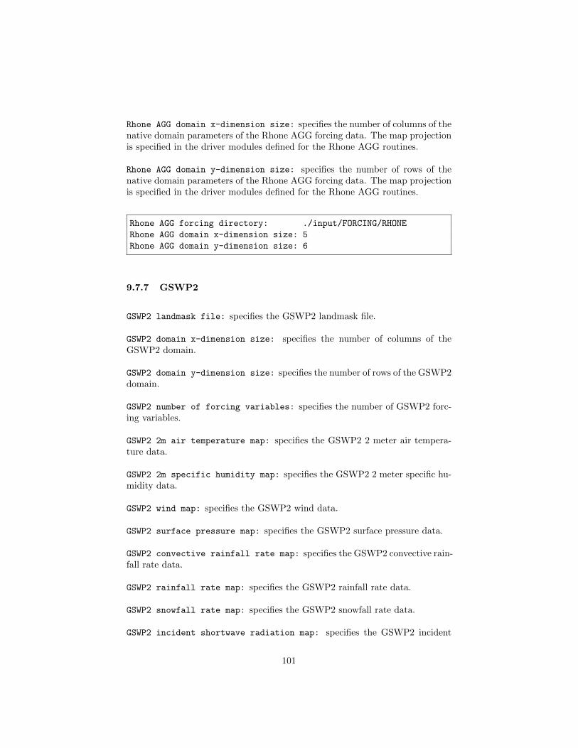
Rhone AGG domain x-dimension size: specifies the number of columns of thenative domain parameters of the Rhone AGG forcing data. The map projectionis specified in the driver modules defined for the Rhone AGG routines.

Rhone AGG domain y-dimension size: specifies the number of rows of thenative domain parameters of the Rhone AGG forcing data. The map projectionis specified in the driver modules defined for the Rhone AGG routines.

Rhone AGG forcing directory: ./input/FORCING/RHONE

Rhone AGG domain x-dimension size: 5

Rhone AGG domain y-dimension size: 6

9.7.7 GSWP2

GSWP2 landmask file: specifies the GSWP2 landmask file.

GSWP2 domain x-dimension size: specifies the number of columns of theGSWP2 domain.

GSWP2 domain y-dimension size: specifies the number of rows of the GSWP2domain.

GSWP2 number of forcing variables: specifies the number of GSWP2 forc-ing variables.

GSWP2 2m air temperature map: specifies the GSWP2 2 meter air tempera-ture data.

GSWP2 2m specific humidity map: specifies the GSWP2 2 meter specific hu-midity data.

GSWP2 wind map: specifies the GSWP2 wind data.

GSWP2 surface pressure map: specifies the GSWP2 surface pressure data.

GSWP2 convective rainfall rate map: specifies the GSWP2 convective rain-fall rate data.

GSWP2 rainfall rate map: specifies the GSWP2 rainfall rate data.

GSWP2 snowfall rate map: specifies the GSWP2 snowfall rate data.

GSWP2 incident shortwave radiation map: specifies the GSWP2 incident

101

shortwave radiation data.

GSWP2 incident longwave radiation map: specifies the GSWP2 incident long-wave radiation data.

GSWP2 landmask file: ./input/gswp2data/Fixed/landmask_gswp.nc

GSWP2 domain x-dimension size: 360

GSWP2 domain y-dimension size: 150

GSWP2 number of forcing variables: 10

GSWP2 2m air temperature map: ./input/gswp2data/Tair_cru/Tair_cru

GSWP2 2m specific humidity map: ./input/gswp2data/Qair_cru/Qair_cru

GSWP2 wind map: ./input/gswp2data/Wind_ncep/Wind_ncep

GSWP2 surface pressure map: ./input/gswp2data/PSurf_ecor/PSurf_ecor

GSWP2 convective rainfall rate map: ./input/gswp2data/Rainf_C_gswp/Rainf_C_gswp

GSWP2 rainfall rate map: ./input/gswp2data/Rainf_gswp/Rainf_gswp

GSWP2 snowfall rate map: ./input/gswp2data/Snowf_gswp/Snowf_gswp

GSWP2 incident shortwave radiation map: ./input/gswp2data/SWdown_srb/SWdown_srb

GSWP2 incident longwave radiation map: ./input/gswp2data/LWdown_srb/LWdown_srb

9.7.8 GMAO GLDAS

GLDAS forcing directory: specifies the location of the GMAO GLDAS forc-ing files.

GLDAS forcing directory: ../FORCING/GLDAS_GMAO/

9.7.9 GFS

GFS forcing directory: specifies the location of the GFS forcing files.

GFS domain x-dimension size: specifies the number of columns of the nativedomain parameters of the GFS forcing data. The map projection is specified inthe driver modules defined for the GFS routines.

GFS domain y-dimension size: specifies the number of rows of the nativedomain parameters of the GFS forcing data. The map projection is specified inthe driver modules defined for the GFS routines.

GFS number of forcing variables: specifies the number of forcing variablesprovided by GFS at the model initialization step.

102

GFS forcing directory: ./input/FORCING/GFS/

GFS domain x-dimension size: 512

GFS domain y-dimension size: 256

GFS number of forcing variables: 10

9.7.10 MERRA-Land

MERRA-Land forcing directory: specifies the location of the MERRA-Landforcing files.

MERRA-Land use lowest model level forcing: specifies whether to use thelowest model level forcing. Acceptable values are:

Value Description0 Do not use the lowest model level forcing.1 Use the lowest model level forcing.

MERRA-Land forcing directory:

MERRA-Land use lowest model level forcing:

9.7.11 MERRA2

MERRA2 forcing directory: specifies the location of the MERRA2 forcingfiles.

Please note that MERRA2 forcing data are not currently available to externalusers. They should become available in July 2015.

MERRA2 use lowest model level forcing: specifies whether to use the low-est model level forcing. Acceptable values are:

Value Description0 Do not use the lowest model level forcing.1 Use the lowest model level forcing.

MERRA2 use corrected total precipitation: specifies whether to use thebias corrected total precipitation. Acceptable values are:

103

Value Description0 Do not use the bias corrected total precipitation.1 Use the bias corrected total precipitation.

MERRA2 forcing directory:

MERRA2 use lowest model level forcing:

MERRA2 use corrected total precipitation:

9.7.12 GSWP1

GSWP1 forcing directory: specifies the location of the GSWP1 forcing files.

GSWP1 domain x-dimension size: specifies the number of columns of the na-tive domain parameters of the GSWP1 forcing data. The map projection isspecified in the driver modules defined for the GSWP1 routines.

GSWP1 domain y-dimension size: specifies the number of rows of the nativedomain parameters of the GSWP1 forcing data. The map projection is specifiedin the driver modules defined for the GSWP1 routines.

GSWP1 number of forcing variables: specifies the number of forcing vari-ables provided by GSWP1 at the model initialization step.

GSWP1 forcing directory: ./input/FORCING/GSWP1

GSWP1 domain x-dimension size: 360

GSWP1 domain y-dimension size: 150

GSWP1 number of forcing variables: 9

9.8 Supplemental forcings

9.8.1 AGRMET radiation (latlon)

AGRRAD forcing directory: specifies the directory containing AGRMET ra-diation data.

AGRRAD forcing directory: ./input/FORCING/AGRRAD

104

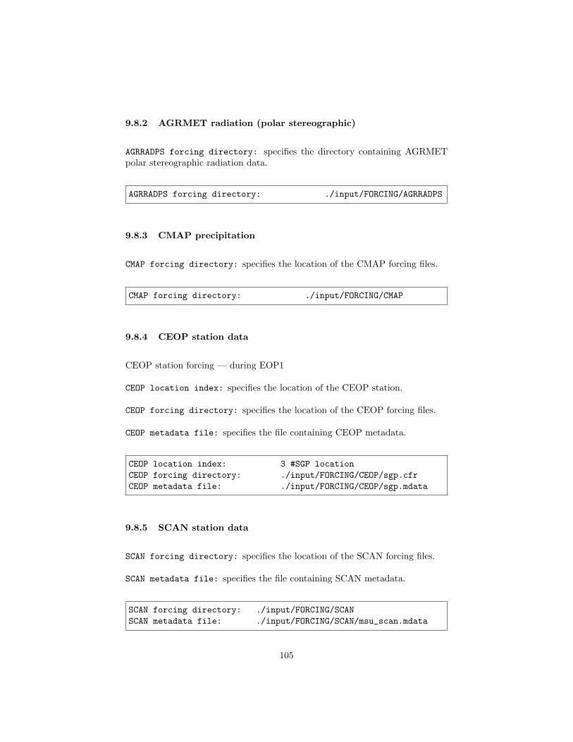
9.8.2 AGRMET radiation (polar stereographic)

AGRRADPS forcing directory: specifies the directory containing AGRMETpolar stereographic radiation data.

AGRRADPS forcing directory: ./input/FORCING/AGRRADPS

9.8.3 CMAP precipitation

CMAP forcing directory: specifies the location of the CMAP forcing files.

CMAP forcing directory: ./input/FORCING/CMAP

9.8.4 CEOP station data

CEOP station forcing — during EOP1

CEOP location index: specifies the location of the CEOP station.

CEOP forcing directory: specifies the location of the CEOP forcing files.

CEOP metadata file: specifies the file containing CEOP metadata.

CEOP location index: 3 #SGP location

CEOP forcing directory: ./input/FORCING/CEOP/sgp.cfr

CEOP metadata file: ./input/FORCING/CEOP/sgp.mdata

9.8.5 SCAN station data

SCAN forcing directory: specifies the location of the SCAN forcing files.

SCAN metadata file: specifies the file containing SCAN metadata.

SCAN forcing directory: ./input/FORCING/SCAN

SCAN metadata file: ./input/FORCING/SCAN/msu_scan.mdata

105

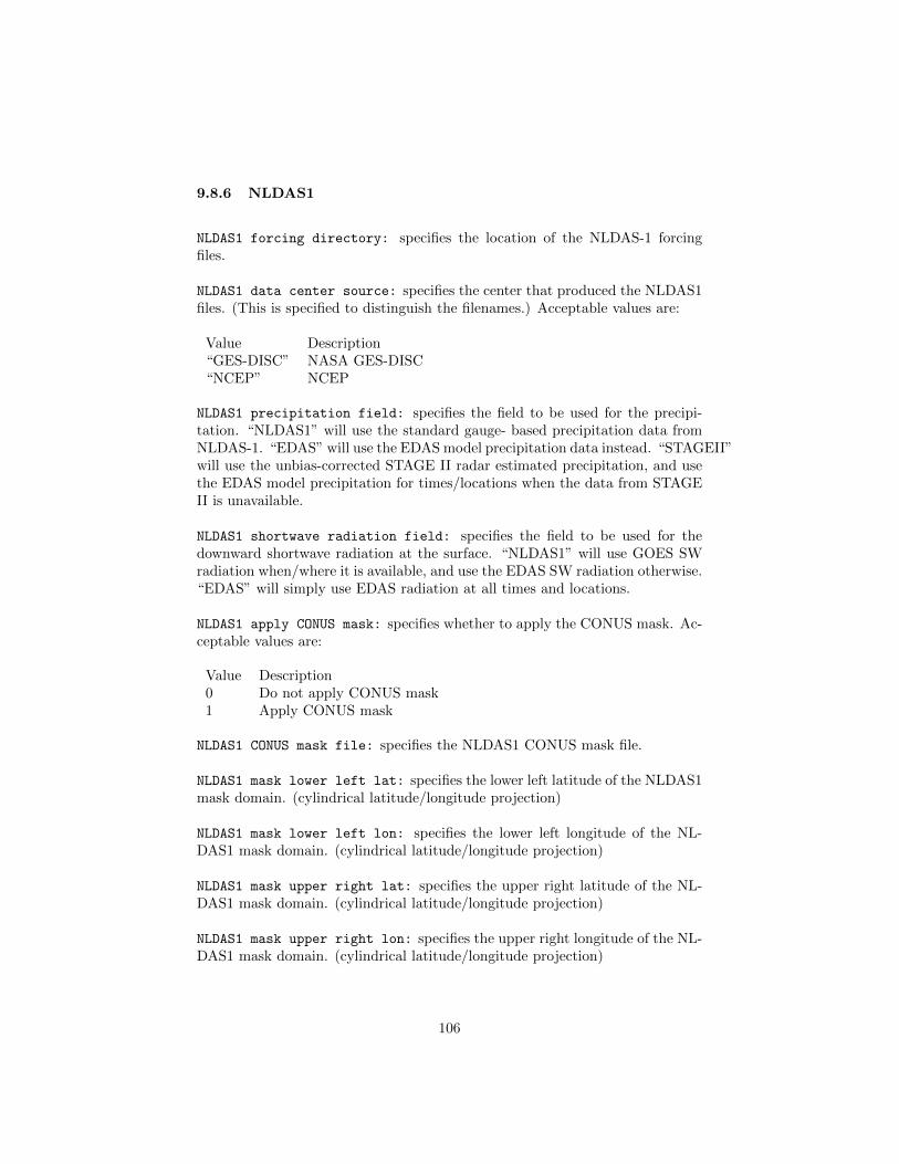
9.8.6 NLDAS1

NLDAS1 forcing directory: specifies the location of the NLDAS-1 forcingfiles.

NLDAS1 data center source: specifies the center that produced the NLDAS1files. (This is specified to distinguish the filenames.) Acceptable values are:

Value Description“GES-DISC” NASA GES-DISC“NCEP” NCEP

NLDAS1 precipitation field: specifies the field to be used for the precipi-tation. “NLDAS1” will use the standard gauge- based precipitation data fromNLDAS-1. “EDAS” will use the EDAS model precipitation data instead. “STAGEII”will use the unbias-corrected STAGE II radar estimated precipitation, and usethe EDAS model precipitation for times/locations when the data from STAGEII is unavailable.

NLDAS1 shortwave radiation field: specifies the field to be used for thedownward shortwave radiation at the surface. “NLDAS1” will use GOES SWradiation when/where it is available, and use the EDAS SW radiation otherwise.“EDAS” will simply use EDAS radiation at all times and locations.

NLDAS1 apply CONUS mask: specifies whether to apply the CONUS mask. Ac-ceptable values are:

Value Description0 Do not apply CONUS mask1 Apply CONUS mask

NLDAS1 CONUS mask file: specifies the NLDAS1 CONUS mask file.

NLDAS1 mask lower left lat: specifies the lower left latitude of the NLDAS1mask domain. (cylindrical latitude/longitude projection)

NLDAS1 mask lower left lon: specifies the lower left longitude of the NL-DAS1 mask domain. (cylindrical latitude/longitude projection)

NLDAS1 mask upper right lat: specifies the upper right latitude of the NL-DAS1 mask domain. (cylindrical latitude/longitude projection)

NLDAS1 mask upper right lon: specifies the upper right longitude of the NL-DAS1 mask domain. (cylindrical latitude/longitude projection)

106

NLDAS1 mask resolution (dx): specifies the resolution of the NLDAS1 maskdomain along the east-west direction.

NLDAS1 mask resolution (dy): specifies the resolution of the NLDAS1 maskdomain along the north-south direction.

NLDAS1 forcing directory: ./input/FORCING/NLDAS1

NLDAS1 data center source: "GES-DISC"

NLDAS1 precipitation field: NLDAS1

NLDAS1 shortwave radiation field: NLDAS1

NLDAS1 apply CONUS mask: 0

NLDAS1 CONUS mask file:

NLDAS1 mask lower left lat: 25.0625

NLDAS1 mask lower left lon: -124.9375

NLDAS1 mask upper right lat: 52.9375

NLDAS1 mask upper right lon: -67.0625

NLDAS1 mask resolution (dx): 0.125

NLDAS1 mask resolution (dy): 0.125

9.8.7 NLDAS2

NLDAS2 forcing directory: specifies the location of the NLDAS2 forcingfiles.

NLDAS2 data center source: specifies the center that produced the NLDAS2files. (This is specified to distinguish the filenames.) Acceptable values are:

Value Description“GES-DISC” NASA GES-DISC“NCEP” NCEP

NLDAS2 use model level data: specifies whether or not to read in the modellevel data (instead of 2/10m fields) from the NLDAS2 forcing dataset (will openup and read “B” files). This data is at the height of the NARR lowest modellevel.

Note that this will read in “Height of Atmospheric Forcing” and “Surface Ex-change Coefficient for Heat”. You must make sure that they are included inyour forcing variables list file. Acceptable values are:


107

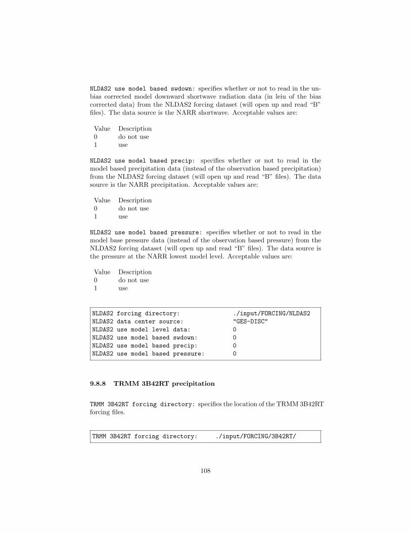
NLDAS2 use model based swdown: specifies whether or not to read in the un-bias corrected model downward shortwave radiation data (in leiu of the biascorrected data) from the NLDAS2 forcing dataset (will open up and read “B”files). The data source is the NARR shortwave. Acceptable values are:


NLDAS2 use model based precip: specifies whether or not to read in themodel based precipitation data (instead of the observation based precipitation)from the NLDAS2 forcing dataset (will open up and read “B” files). The datasource is the NARR precipitation. Acceptable values are:


NLDAS2 use model based pressure: specifies whether or not to read in themodel base pressure data (instead of the observation based pressure) from theNLDAS2 forcing dataset (will open up and read “B” files). The data source isthe pressure at the NARR lowest model level. Acceptable values are:


NLDAS2 forcing directory: ./input/FORCING/NLDAS2

NLDAS2 data center source: "GES-DISC"

NLDAS2 use model level data: 0

NLDAS2 use model based swdown: 0

NLDAS2 use model based precip: 0

NLDAS2 use model based pressure: 0

9.8.8 TRMM 3B42RT precipitation

TRMM 3B42RT forcing directory: specifies the location of the TRMM 3B42RTforcing files.

TRMM 3B42RT forcing directory: ./input/FORCING/3B42RT/

108

TRMM 3B42RTV7 forcing directory: specifies the location of the TRMM 3B42RTVersion 7 forcing files.

TRMM 3B42RTV7 forcing directory: ../MET_FORCING/3B42RT-V7/

9.8.9 TRMM 3B42V6 precipitation

TRMM 3B42V6 timestep: specifies the timestep for reading the TRMM 3B42V6data.


TRMM 3B42V6 forcing directory: specifies the location of the TRMM 3B42V6forcing files.

TRMM 3B42V6 forcing directory: ./input/FORCING/3B42V6/

TRMM 3B42V6 timestep: 1hr

9.8.10 TRMM 3B42V7 precipitation

TRMM 3B42V7 timestep: specifies the timestep for reading the TRMM 3B42V7data.


TRMM 3B42V7 forcing directory: specifies the location of the TRMM 3B42V7forcing files.

TRMM 3B42V7 forcing directory: ./input/FORCING/3B42V7/

TRMM 3B42V7 timestep: 1hr

9.8.11 CMORPH precipitation

CMORPH forcing directory: specifies the location of the CMORPH precipi-tation forcing files.

109

CMORPH forcing directory: ./input/FORCING/CMORPH/

9.8.12 Stage II precipitation

STAGE2 forcing directory: specifies the location of the STAGE2 forcing files.

STAGE2 forcing directory: ./input/FORCING/STII

9.8.13 Stage IV precipitation

STAGE4 forcing directory: specifies the location of the STAGE4 forcing files.

STAGE4 forcing directory: ./input/FORCING/STIV

9.8.14 NARR

NARR forcing directory: specifies the location of the NARR forcing files.

NARR domain x-dimension size: specifies the number of columns of the na-tive domain parameters of the NARR forcing data.

NARR domain y-dimension size: specifies the number of rows of the nativedomain parameters of the NARR forcing data.

NARR domain y-dimension size: specifies the number of rows of the nativedomain parameters of the NARR forcing data.

NARR domain z-dimension size: specifies the number of atmospheric profilesin the NARR forcing data.

NARR forcing directory: ./input/Code/NARR/

NARR domain x-dimension size: 768

NARR domain y-dimension size: 386

NARR domain z-dimension size: 30

110

9.8.15 RFE2Daily

RFE2Daily forcing directory: specifies the location of the RFE2Daily forc-ing files.

RFE2Daily time offset: specifiles the time offset for the RFE2Daily forcingdata, in hours. This adjusts when LIS will read the RFE2Daily precipitationdata. For general use, the data should be read at hour 6z, but for use byGeoWRSI, the data should be read at hour 0z.

RFE2Daily forcing directory: ./input/MET_FORCING/RFE2.0_CPC/Africa/

RFE2Daily time offset: 0 # for use by GeoWRSI

9.8.16 PET USGS

USGS PET forcing directory: specifies the location of the PET USGS forcingfiles.

USGS PET forcing type: specifies the choice for PET forcing data type. Ac-ceptable values are:

Value Descriptioncurrent Retrospective or current time-based PET filesclimatology Climatology-based PET files

USGS PET forcing directory: ./PET_USGS

9.8.17 RFE2 data bias corrected to GDAS

RFE2gdas forcing directory: specifies the location of the RFE2gdas forcingfiles.

RFE2gdas forcing directory:

111

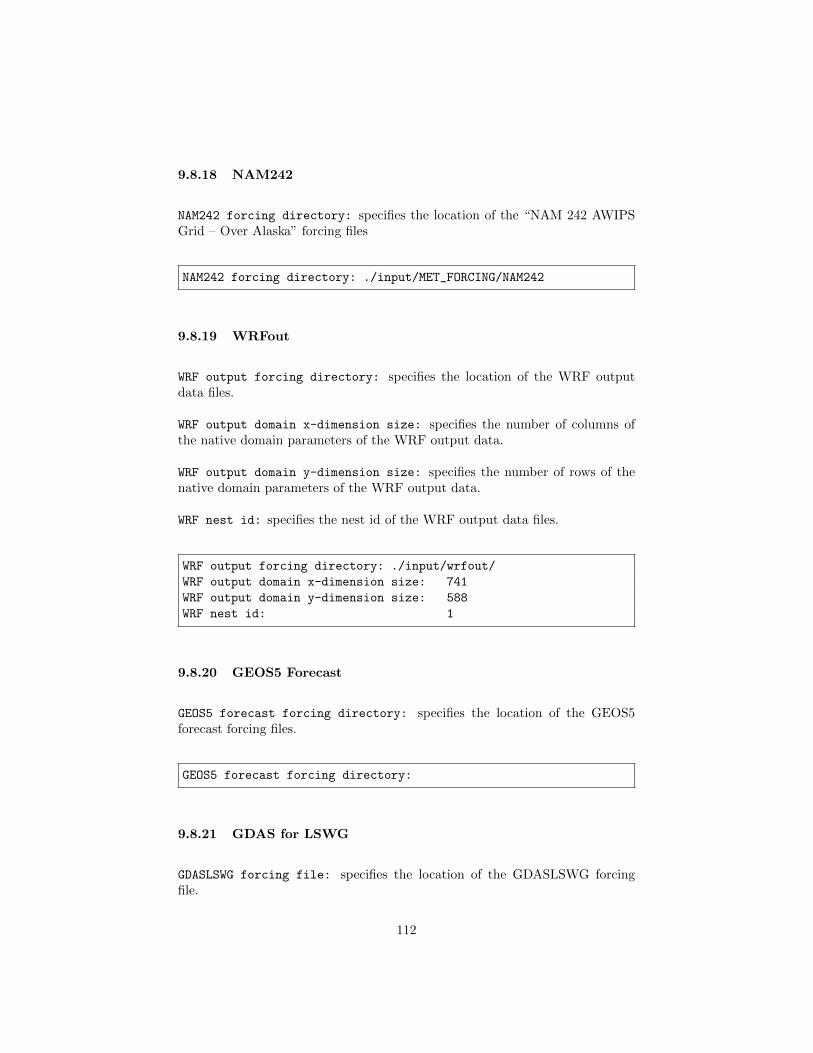
9.8.18 NAM242

NAM242 forcing directory: specifies the location of the “NAM 242 AWIPSGrid – Over Alaska” forcing files

NAM242 forcing directory: ./input/MET_FORCING/NAM242

9.8.19 WRFout

WRF output forcing directory: specifies the location of the WRF outputdata files.

WRF output domain x-dimension size: specifies the number of columns ofthe native domain parameters of the WRF output data.

WRF output domain y-dimension size: specifies the number of rows of thenative domain parameters of the WRF output data.

WRF nest id: specifies the nest id of the WRF output data files.

WRF output forcing directory: ./input/wrfout/

WRF output domain x-dimension size: 741

WRF output domain y-dimension size: 588

WRF nest id: 1

9.8.20 GEOS5 Forecast

GEOS5 forecast forcing directory: specifies the location of the GEOS5forecast forcing files.

GEOS5 forecast forcing directory:

9.8.21 GDAS for LSWG

GDASLSWG forcing file: specifies the location of the GDASLSWG forcingfile.

112

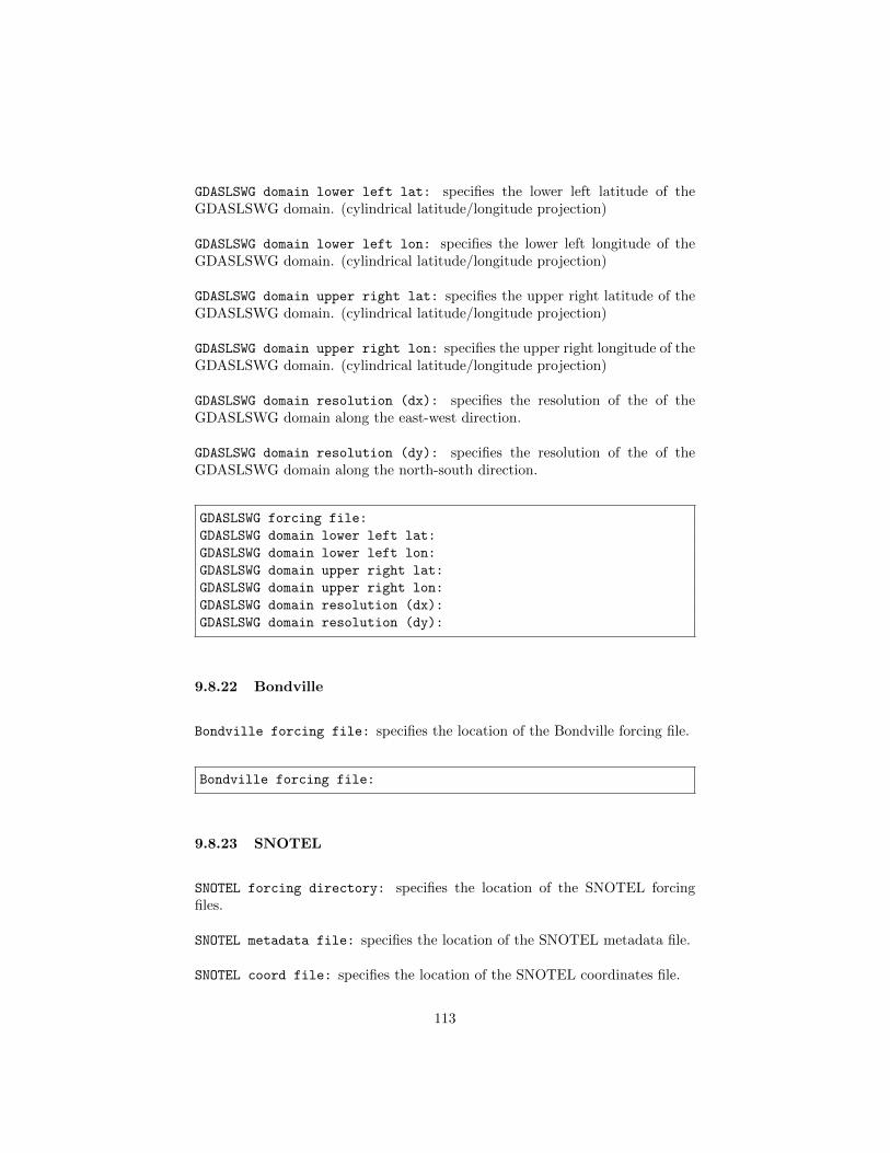
GDASLSWG domain lower left lat: specifies the lower left latitude of theGDASLSWG domain. (cylindrical latitude/longitude projection)

GDASLSWG domain lower left lon: specifies the lower left longitude of theGDASLSWG domain. (cylindrical latitude/longitude projection)

GDASLSWG domain upper right lat: specifies the upper right latitude of theGDASLSWG domain. (cylindrical latitude/longitude projection)

GDASLSWG domain upper right lon: specifies the upper right longitude of theGDASLSWG domain. (cylindrical latitude/longitude projection)

GDASLSWG domain resolution (dx): specifies the resolution of the of theGDASLSWG domain along the east-west direction.

GDASLSWG domain resolution (dy): specifies the resolution of the of theGDASLSWG domain along the north-south direction.

GDASLSWG forcing file:

GDASLSWG domain lower left lat:

GDASLSWG domain lower left lon:

GDASLSWG domain upper right lat:

GDASLSWG domain upper right lon:

GDASLSWG domain resolution (dx):

GDASLSWG domain resolution (dy):

9.8.22 Bondville

Bondville forcing file: specifies the location of the Bondville forcing file.

Bondville forcing file:

9.8.23 SNOTEL

SNOTEL forcing directory: specifies the location of the SNOTEL forcingfiles.

SNOTEL metadata file: specifies the location of the SNOTEL metadata file.

SNOTEL coord file: specifies the location of the SNOTEL coordinates file.

113

SNOTEL forcing directory:

SNOTEL metadata file:

SNOTEL coord file:

9.8.24 COOP

COOP forcing directory: specifies the location of the COOP forcing files.

COOP metadata file: specifies the location of the COOP metadata file.

COOP coord file: specifies the location of the COOP coordinate file.

COOP forcing directory:

COOP metadata file:

COOP coord file:

9.8.25 VIC processed forcing

This is used by the LIS development team to support debugging VIC withinLIS. One must first run stand-alone VIC, configured to output its forcing data.Then one must grid the output forcing data into a format understood by LIS.

VIC forcing directory: specifies the location of the VIC processed forcingfiles.

VIC forcing interval: specifies the frequency of the VIC processed forcingdata, in seconds.

VIC forcing domain lower left lat: specifies the lower left latitude of theVIC processed forcing data. (cylindrical latitude/longitude projection)

VIC forcing domain lower left lon: specifies the lower left longitude ofthe VIC processed forcing data. (cylindrical latitude/longitude projection)

VIC forcing domain upper right lat: specifies the upper right latitude ofthe VIC processed forcing data. (cylindrical latitude/longitude projection)

VIC forcing domain upper right lon: specifies the upper right longitude ofthe VIC processed forcing data. (cylindrical latitude/longitude projection)

114

VIC forcing domain resolution (dx): specifies the resolution of the of theVIC processed forcing data along the east-west direction.

VIC forcing domain resolution (dy): specifies the resolution of the of theVIC processed forcing data along the north-south direction.

VIC NC: specifies the number of columns of the VIC processed forcing data.

VIC NR: specifies the number of rows of the VIC processed forcing data.

VIC forcing directory:

VIC forcing interval:

VIC forcing domain lower left lat:

VIC forcing domain lower left lon:

VIC forcing domain upper right lat:

VIC forcing domain upper right lon:

VIC forcing domain resolution (dx):

VIC forcing domain resolution (dy):

VIC NC:

VIC NR:

9.8.26 PALS station

PALS met forcing directory: specifies the location of the PALS station forc-ing files.

PALS met forcing station name: specifies the name of the PALS station.

PALS met forcing data start year: specifies the starting year of the PALSstation data.

PALS met forcing data start month: specifies the starting month of thePALS station data.

PALS met forcing data start day: specifies the starting day of the PALSstation data.

PALS met forcing data start hour: specifies the starting hour of the PALSstation data.

PALS met forcing data start minute: specifies the starting minute of thePALS station data.

115

PALS met forcing data start second: specifies the starting second of thePALS station data.

PALS met forcing directory:

PALS met forcing station name:

PALS met forcing data start year:

PALS met forcing data start month:

PALS met forcing data start day:

PALS met forcing data start hour:

PALS met forcing data start minute:

PALS met forcing data start second:

9.8.27 PILDAS

PILDAS forcing directory: specifies the location of the PILDAS forcing files.

PILDAS forcing version: specifies the version of the PILDAS forcing data.

PILDAS forcing use lowest model level fields: specifies whether to usethe lowest model level fields. Acceptable values are:

Value Description0 Do not use lowest level1 Use lowest level

PILDAS forcing directory:

PILDAS forcing version:

PILDAS forcing use lowest model level fields:

9.8.28 RDHM356

RDHM precipitation forcing directory: specifies the location of the RDHMprecipitation forcing files.

RDHM temperature forcing directory: specifies the location of the RDHMtemperature forcing files.

RDHM precipitation scale factor: specifies the RDHM precipitation scalefactor, which is used to scale the integer type XMRG data into real numberrepresenting precipitation amount.

116

RDHM precipitation interval: specifies the frequency of the precipitationforcing data, in seconds.

RDHM temperature interval: specifies the frequency of the temperature forc-ing data, in seconds.

RDHM run window lower left hrap y: lower left HRAP Y coordinate of rundomain

RDHM run window lower left hrap x: lower left HRAP X coordinate of rundomain

RDHM run window upper right hrap y: upper right HRAP Y coordinate ofrun domain

RDHM run window upper right hrap x: upper right HRAP X coordinate ofrun domain

RDHM run window hrap resolution: spatial resolution (in HRAP unit) of rundomain

RDHM temperature undefined value: specifies the undefined value for thetemperature forcing data.

RDHM precipitation undefined value: specifies the undefined value for theprecipitation forcing data.

RDHM constant wind speed: Constant wind speed (m/s) for entire run domain

RDHM precipitation forcing directory: ../testcase/precip

RDHM temperature forcing directory: ../testcase/tair

RDHM precipitation scale factor: 1.0

RDHM precipitation interval: 3600

RDHM temperature interval: 3600

RDHM run window lower left hrap y: 48

RDHM run window lower left hrap x: 17

RDHM run window upper right hrap y: 821

RDHM run window upper right hrap x: 1059

RDHM run window hrap resolution: 1.0

RDHM temperature undefined value: -1.0

RDHM precipitation undefined value: -1.0

RDHM constant wind speed: 4.0

Generated metforcing directory: specifies the location of the LDT gener-

117

ated meteorological forcing files. Files generated in LDT are in netCDF format,and they are automatically loaded and handled by the LIS-7 reader.

Generated metforcing directory: ./LDT_OUTPUT/

9.9 Land surface models

9.9.1 Forcing only – Template

TEMPLATE model timestep: specifies the timestep for the run. The templateLSM is not a model; rather, it is a placeholder for a model. It demonstrates thehooks that are needed to add a land surface model into LIS. This “LSM” is alsoused to run LIS with the purpose of only processing and writing forcing data.


TEMPLATE model timestep: 1hr

9.9.2 NCEP’s Noah-2.7.1

Noah.2.7.1 model timestep: specifies the timestep for the run.


For a nested domain, the timesteps for each nest should be specified with whitespaces as the delimiter. If two domains (one subnest) are employed, the firstone using 900 seconds and the second one using 3600 seconds as the timestep,the model timesteps are specified as:

E.g.: Noah.2.7.1 model timestep: 15mn 60mn

Noah.2.7.1 restart output interval: defines the restart writing intervalfor Noah-2.7.1. The typical value used in the LIS runs is 24 hours (1da).


Noah.2.7.1 restart file: specifies the Noah-2.7.1 active restart file.

118

Noah.2.7.1 vegetation parameter table: specifies the Noah-2.7.1 static veg-etation parameter table file.

Noah.2.7.1 soil parameter table: specifies the Noah-2.7.1 soil parameterfile.

Noah.2.7.1 use PTF for mapping soil properties: specifies if pedotrans-fer functions are to be used for mapping soil properties (0-do not use, 1-use).

Noah.2.7.1 number of vegetation parameters: specifies the number of staticvegetation parameters specified for each veg type.

Noah.2.7.1 soils scheme: specifies the soil mapping scheme used. Accept-able values are:

Value Description1 Zobler2 STATSGO

Noah.2.7.1 number of soil classes: specifies the number of soil classes inthe above mapping scheme. Acceptable values are:


Noah.2.7.1 number of soil layers: specifies the number of soil layers. Thetypical value used in Noah-2.7.1 is 4.

Noah.2.7.1 layer thicknesses: specifies the thickness (in meters) of each ofthe Noah-2.7.1 soil layers (top layer to bottom layer).

Noah.2.7.1 initial skin temperature: specifies the initial skin tempera-ture in Kelvin used in the cold start runs.

Noah.2.7.1 initial soil temperatures: specifies the initial soil tempera-ture (for all layers, top to bottom) in Kelvin used in the cold start runs.

Noah.2.7.1 initial total soil moistures: specifies the initial total volu-metric soil moistures (for all layers, top to bottom) used in the cold start runs.

(units m3

m3 )

Noah.2.7.1 initial liquid soil moistures: specifies the initial liquid vol-umetric soil moistures (for all layers, top to bottom) used in the cold start runs.

(units m3

m3 )

119

Noah.2.7.1 initial canopy water: specifies the initial canopy water (m).

Noah.2.7.1 initial snow depth: specifies the initial snow depth (m).

Noah.2.7.1 initial snow equivalent: specifies the initial snow water equiv-alent (m).

Noah.2.7.1 reference height for forcing T and q: specifies the heightin meters of air temperature and specific humidity forcings.

Noah.2.7.1 reference height for forcing u and v: specifies the heightin meters of u and v wind forcings.

Noah.2.7.1 reinitialize parameters from OPTUE output: specifies whetherto reinitialize parameters from OPTUE output. Defaults to 0.

Noah.2.7.1 parameter restart file (from OPTUE): specifies the restart fileto use to reinitialize parameters. Only used when Noah.2.7.1 reinitialize

parameters from OPTUE output: is set to 1.

Noah.2.7.1 model timestep: 15mn

Noah.2.7.1 restart output interval: 1mo

Noah.2.7.1 restart file: ./LIS.E111.200401210000.d01.Noah271rst

Noah.2.7.1 vegetation parameter table: ../../noah271_parms/noah.vegparms_UMD.txt

Noah.2.7.1 soil parameter table: ../../noah271_parms/noah.soilparms_STATSGO-FAO.txt

Noah.2.7.1 use PTF for mapping soil properties: 0

Noah.2.7.1 number of vegetation parameters: 7

Noah.2.7.1 soils scheme: 2 # 1-Zobler; 2-STATSGO

Noah.2.7.1 number of soil classes: 16 # 9 for Zobler

Noah.2.7.1 number of soil layers: 4

Noah.2.7.1 layer thicknesses: 0.1 0.3 0.6 1.0

Noah.2.7.1 initial skin temperature: 290.0000 # Kelvin

Noah.2.7.1 initial soil temperatures: 290.0000 290.0000 290.0000 290.0000 # Kelvin

Noah.2.7.1 initial total soil moistures: 0.2000000 0.2000000 0.2000000 0.2000000 # volumetric (m3 m-3)

Noah.2.7.1 initial liquid soil moistures: 0.2000000 0.2000000 0.2000000 0.2000000 # volumetric (m3 m-3)

Noah.2.7.1 initial canopy water: 0.0 # depth (m)

Noah.2.7.1 initial snow depth: 0.0 # depth (m)

Noah.2.7.1 initial snow equivalent: 0.0 # SWE depth (m)

Noah.2.7.1 reference height for forcing T and q: 20.0

Noah.2.7.1 reference height for forcing u and v: 20.0

120

9.9.3 NCAR’s Noah-3.2

Noah.3.2 model timestep: specifies the timestep for the run.



E.g.: Noah.3.2 model timestep: 15mn 60mn

Noah.3.2 restart output interval: defines the restart writing interval forNoah-3.2. The typical value used in the LIS runs is 24 hours (1da).


Noah.3.2 restart file: specifies the Noah-3.2 active restart file.

Noah.3.2 vegetation parameter table: specifies the Noah-3.2 static vege-tation parameter table file.

Noah.3.2 soil parameter table: specifies the Noah-3.2 soil parameter file.

Noah.3.2 general parameter table: specifies the Noah-3.2 general parame-ter file.

Noah.3.2 use PTF for mapping soil properties: specifies if pedotransferfunctions are to be used for mapping soil properties (0-do not use, 1-use).

Noah.3.2 soils scheme: specifies the soil mapping scheme used. Acceptablevalues are:


Noah.3.2 number of soil layers: specifies the number of soil layers. Thetypical value used in Noah is 4.

Noah.3.2 layer thicknesses: specifies the thickness (in meters) of each ofthe Noah-3.2 soil layers (top layer to bottom layer).

Noah.3.2 use distributed soil depth map: specifies whether to use a dis-

121

tributed soil depth map. Defaults to 0.

Noah.3.2 use distributed root depth map: specifies whether to use a dis-tributed root depth map. Defaults to 0.

Noah.3.2 initial skin temperature: specifies the initial skin temperaturein Kelvin used in the cold start runs.

Noah.3.2 initial soil temperatures: specifies the initial soil temperature(for all layers, top to bottom) in Kelvin used in the cold start runs.

Noah.3.2 initial total soil moistures: specifies the initial total volu-metric soil moistures (for all layers, top to bottom) used in the cold start runs.

(units m3

m3 )

Noah.3.2 initial liquid soil moistures: specifies the initial liquid volu-metric soil moistures (for all layers, top to bottom) used in the cold start runs.

(units m3

m3 )

Noah.3.2 initial canopy water: specifies the initial canopy water (m).

Noah.3.2 initial snow depth: specifies the initial snow depth (m).

Noah.3.2 initial snow equivalent: specifies the initial snow water equiva-lent (m).

Noah.3.2 fixed max snow albedo: specifies a fixed maximum snow albedo(fraction, 0.0 to 1.0) for all grid points. This value will only be used if “fixed”is chosen for Max snow albedo data source.

Noah.3.2 fixed deep soil temperature: specifies a fixed deep soil temper-ature (Kelvin) for all grid points. Entering a value of 0.0 will have the code usethe deep soil temperature from the LDT-generated LIS domain and parameter

data file.

Noah.3.2 fixed vegetation type: specifies a fixed vegetation type index forall grid points. Entering a value of 0 will not fix the vegetation types, and thecode will use the Landcover data source information instead.

Noah.3.2 fixed soil type: specifies a fixed soil type index for all grid points.Entering a value of 0 will not fix the soil types, and the code will use the Soil

texture data source information instead.

Noah.3.2 fixed slope type: specifies a fixed slope type index for all gridpoints. Entering a value of 0 will not fix the slope index types, and the code

122

will use the Slope data source information instead.

Noah.3.2 sfcdif option: specifies whether to use the updated SFCDIF rou-tine in Noah-3.2, or to use the previous SFCDIF routine. The typical option isto use the updated SFCDIF routine (option = 1).

Noah.3.2 z0 veg-type dependence option: specifies whether to use the veg-etation type dependent roughness height option on the CZIL parameter in theSFCDIF routine. The typical option in Noah-3.2 is not use this dependence(option = 0).

Noah.3.2 greenness fraction: specifies a monthly (January to December)greenness vegetation fraction for all grid points. These values are used only ifthe Greenness data source option is set to “none”.

Noah.3.2 background albedo: specifies a monthly background (snow-free)albedo for all grid points. These values are only used for an initial conditioncalculation, and only if the Albedo data source option is set to “none”. Afterthe first timestep, these values are not used.

Noah.3.2 background roughness length: specifies a monthly background(snow-free) roughness length. These values are used only for an initial con-dition calculation and are not used after the first timestep.

Noah.3.2 reference height for forcing T and q: specifies the height inmeters of air temperature and specific humidity forcings.

Noah.3.2 reference height for forcing u and v: specifies the height inmeters of u and v wind forcings.

Noah.3.2 model timestep: 15mn

Noah.3.2 restart output interval: 1mo

Noah.3.2 restart file: LIS.E111.200805140000.d01.Noah32rst

Noah.3.2 vegetation parameter table: ../../noah32_parms/VEGPARM.TBL

Noah.3.2 soil parameter table: ../../noah32_parms/SOILPARM.TBL

Noah.3.2 general parameter table: ../../noah32_parms/GENPARM.TBL

Noah.3.2 use PTF for mapping soil properties: 0

Noah.3.2 soils scheme: 2 # 1-Zobler; 2-STATSGO

Noah.3.2 number of soil layers: 4

Noah.3.2 layer thicknesses: 0.1 0.3 0.6 1.0

Noah.3.2 use distributed soil depth map: 0 # 0 - do not use; 1 - use map

Noah.3.2 use distributed root depth map: 0 # 0 - do not use; 1 - use map

Noah.3.2 initial skin temperature: 290.0000 # Kelvin

Noah.3.2 initial soil temperatures: 290.0000 290.0000 290.0000 290.0000 # Kelvin

Noah.3.2 initial total soil moistures: 0.2000000 0.2000000 0.2000000 0.2000000 # volumetric (m3 m-3)

123

Noah.3.2 initial liquid soil moistures: 0.2000000 0.2000000 0.2000000 0.2000000 # volumetric (m3 m-3)

Noah.3.2 initial canopy water: 0.0 # depth (m)

Noah.3.2 initial snow depth: 0.0 # depth (m)

Noah.3.2 initial snow equivalent: 0.0 # SWE depth (m)

Noah.3.2 fixed max snow albedo: 0.0 # fraction; 0.0 - do not fix

Noah.3.2 fixed deep soil temperature: 0.0 # Kelvin; 0.0 - do not fix

Noah.3.2 fixed vegetation type: 0 # 0 - do not fix

Noah.3.2 fixed soil type: 0 # 0 - do not fix

Noah.3.2 fixed slope type: 0 # 0 - do not fix

Noah.3.2 sfcdif option: 1 # 0 - previous SFCDIF; 1 - updated SFCDIF

Noah.3.2 z0 veg-type dependence option: 0 # 0 - off; 1 - on; dependence of CZIL in SFCDIF

# Green vegetation fraction - by month

# - used only if "Greenness data source" above is zero

Noah.3.2 greenness fraction: 0.01 0.02 0.07 0.17 0.27 0.58 0.93 0.96 0.65 0.24 0.11 0.02

# Background (i.e., snow-free) albedo - by month

# - used only for first timestep; subsequent timesteps use

# the values as computed in the previous call to "SFLX"

Noah.3.2 background albedo: 0.18 0.17 0.16 0.15 0.15 0.15 0.15 0.16 0.16 0.17 0.17 0.18

# Background (i.e., snow-free) roughness length (m) - by month



Noah.3.2 background roughness length: 0.020 0.020 0.025 0.030 0.035 0.036 0.035 0.030 0.027 0.025 0.020 0.020

Noah.3.2 reference height for forcing T and q: 20.0 # (m) - negative=use height from forcing data

Noah.3.2 reference height for forcing u and v: 20.0 # (m) - negative=use height from forcing data








124








Noah.3.3 number of soil layers: specifies the number of soil layers. Thetypical value used in Noah is 4.


Noah.3.3 use distributed soil depth map: specifies whether to use a dis-tributed soil depth map. Defaults to 0.





(units m3

m3 )


(units m3

m3 )

125






data file.




Noah.3.3 fixed slope type: specifies a fixed slope type index for all gridpoints. Entering a value of 0 will not fix the slope index types, and the codewill use the Slope data source information instead.





126


Noah.3.3 reference height for forcing T and q: specifies the height inmeters of air temperature and specific humidity forcings.





































127



















Noah.3.6 number of soil layers: specifies the number of soil layers. The

128

typical value used in Noah is 4.


Noah.3.6 use distributed soil depth map: specifies whether to use a dis-tributed soil depth map. Defaults to 0.





(units m3

m3 )


(units m3

m3 )






data file.


129



Noah.3.6 fixed slope type: specifies a fixed slope type index for all gridpoints. Entering a value of 0 will not fix the slope index types, and the codewill use the Slope data source information instead.



Noah.3.6 Run UA snow-physics option: specifies whether to run the Univer-sity of Arizona (UA) snow-physics option. Either “.true.” or “.false.” should beselected. If “.true.” is given, then the UA snow-physics will be run. If “.false.”is given, then the standard Noah snow-physics will be run instead.




Noah.3.6 reference height for forcing T and q: specifies the height inmeters of air temperature and specific humidity observations.






130























Noah.3.6 Run UA snow-physics option: .false. # ".true." or ".false"














9.9.6 NoahMP 3.6

NOAHMP36 model timestep: specifies the timestep for NoahMP.


131

NOAHMP36 restart output interval: specifies the restart output interval forNoahMP.


NOAHMP36 number of soil layers: specifiles the number of soil layers forNoahMP soil moisture/temperature.

NOAHMP36 number of snow layers: specifies the number of snow layers forNoahMP snow model.

NOAHMP36 landuse tbl name: specifies the file name of the NoahMP vegetationparameter table.

NOAHMP36 soil tbl name: specifies the file name of the NoahMP soil parametertable.

NOAHMP36 gen tbl name: specifies the file name of the NoahMP general pa-rameter table.

NOAHMP36 noahmp tbl name: specifies the file name of the NoahMP multi-physics parameter table.

NOAHMP36 landuse scheme name: specifies the NoahMP landuse scheme name(e.g. USGS, check the NoahMP land use parameter table).

NOAHMP36 soil scheme name: specifies the NoahMP soil scheme name (e.g.STAS, check NoahMP soil parameter table).

NOAHMP36 dveg opt: specifies the vegetation model. Acceptable values are:

Value Description1 prescribed [table LAI, shdfac=FVEG]2 dynamic3 table LAI, calculate FVEG4 table LAI, shdfac=maximum

NOAHMP36 crs opt: specifies the canopy stomatal resistance scheme. Accept-able values are:

Value Description1 Ball-Berry2 Jarvis

NOAHMP36 btr opt: specifies the soil moisture factor for stomatal resitance.Acceptable values are:

132

Value Description1 Noah2 CLM3 SSiB

NOAHMP36 run opt: specifies the runoff and groundwater. Acceptable valuesare:

Value Description1 SIMGM2 SIMTOP3 Schaake964 BATS

NOAHMP36 sfc opt: specifies surface layer drag coefficient. Acceptable valuesare:

Value Description1 M-O2 Chen97

NOAHMP36 frz opt: specifies the supercooled liquid water scheme. Acceptablevalues are:

Value Description1 NY062 Koren99

NOAHMP36 inf opt: specifies the frozen soil permeability scheme. Acceptablevalues are:

Value Description1 NY062 Koren99

NOAHMP36 rad opt: specifies the radiation transfer scheme. Acceptable valuesare:

Value Description1 gap=F(3D,cosz)2 gap=03 gap=1–Fveg

NOAHMP36 alb opt: specifies the snow surface albedo scheme. Acceptable val-ues are:

133

Value Description1 BATS2 CLASS

NOAHMP36 snf opt: specifies the rainfall and snowfall determination scheme.Acceptable values are:

Value Description1 Jordan912 BATS3 Noah

NOAHMP36 tbot opt: specifies the lower boundary of soilu temperature scheme.Acceptable values are:

Value Description1 zero-flux2 Noah

NOAHMP36 stc opt: specifies the snow and soil temperature time scheme. Ac-ceptable values are:

Value Description1 semi-implicit2 fully implicit

NOAHMP36 soil layer thickness: specifies the thicknesses of the NoahMPlayers.

NOAHMP36 sc idx: specifies the NoahMP soil color type, an integer index from1 to 8. Defaults to 4.

NOAHMP36 CZIL option (iz0tlnd): specifes whether to use the Chen adjust-ment of Czil. Defaults to 0. Acceptable values are:


NOAHMP36 restart file: specifies the NoahMP restart file.

NOAHMP36 restart file format: specifies the NoahMP restart file format,default: netcdf

NOAHMP36 initial albold: specifies the NoahMP initial albold (albedo ofprevious time step).

134

NOAHMP36 initial sneqvo: specifies the NoahMP initial snow mass at the lasttime step (mm).

NOAHMP36 initial stc: specifies the NoahMP initial soil temperature.

NOAHMP36 initial sh2o: specifies the NoahMP initial soil moisture (liquidpart).

NOAHMP36 initial smc: specifies the NoahMP initial soil moisture (total).

NOAHMP36 initial tah: specifies the NoahMP initial canopy air temperature(K).

NOAHMP36 initial eah: specifies the NoahMP initial canopy air vapor pres-sure (Pa).

NOAHMP36 initial fwet: specifies the NoahMP initial wetted or snowed frac-tion of canopy.

NOAHMP36 initial canliq: specifies the NoahMP intial intercpted liquid wa-ter (mm).

NOAHMP36 initial canice: specifies the NoahMP initial intercepted ice mass(mm).

NOAHMP36 initial tv: specifies the NoahMP intial vegetation temperature(K).

NOAHMP36 initial tg: specifies the NoahMP intial ground temperature (skintemperature) (K).

NOAHMP36 initial qsnow: specifies the NoahMP intial snowfall on the ground(mm/s).

NOAHMP36 initial snowh: specifies the NoahMP initial snow depth (m).

NOAHMP36 initial sneqv: specifies the NoahMP initial snow water equivalent(mm).

NOAHMP36 initial zwt: specifies the NoahMP initial depth to water table(m).

NOAHMP36 initial wa: specifies the NoahMP initial water storage in aquifer(mm).

NOAHMP36 initial wt: specifies the NoahMP initial water in aquifer and sat-

135

urated soil (mm).

NOAHMP36 initial wslake: specifies the NoahMP intial lake water storage(mm).

NOAHMP36 initial lfmass: specifies the NoahMP intial leaf mass (used onlyfor dveg opt=2) (g/m2).

NOAHMP36 initial rtmass: specifies the NoahMP intial mass of fine roots(g/m2).

NOAHMP36 initial stmass: specifies the NoahMP intial stem mass (g/m2).

NOAHMP36 initial wood: specifies the NoahMP intial mass of wood (includingwoody roots) (g/m2).

NOAHMP36 initial stblcp: specifies the NoahMP intial stable carbon in deepsoil (g/m2).

NOAHMP36 initial fastcp: specifies the NoahMP intial short-lived carbon inshallow soil (g/m2).

NOAHMP36 initial lai: specifies the NoahMP intial leaf area index.

NOAHMP36 initial sai: specifies the NoahMP intial stem area index.

NOAHMP36 initial cm: specifies the NoahMP intial momentum drag coefficient(s/m).

NOAHMP36 initial ch: specifies the NoahMP intial sensible heat exchangecoefficient (s/m).

NOAHMP36 initial tauss: specifies the NoahMP intial snow aging term.

NOAHMP36 initial smcwtd: specifies the NoahMP intial soil water contentbetween bottom of the soil and water table (m3/m3).

NOAHMP36 initial deeprech: specifies the NoahMP intial recharge to or fromthe water table when deep (m).

NOAHMP36 initial rech: specifies the NoahMP intial recharge to or from thewater table when shallow (m).

NOAHMP36 initial zlvl: specifies the NoahMP intial reference height of tem-perature and humidity (m).

136

NOAHMP36 model timestep: "15mn"

NOAHMP36 restart output interval: 1da

NOAHMP36 number of soil layers: 4

NOAHMP36 number of snow layers: 3

NOAHMP36 landuse parameter table: "./input/noahmp_params/VEGPARM.TBL"

NOAHMP36 soil parameter table: "./input/noahmp_params/SOILPARM.TBL"

NOAHMP36 general parameter table: "./input/noahmp_params/GENPARM.TBL"

NOAHMP36 MP parameter table: "./input/noahmp_params/MPTABLE.TBL"

NOAHMP36 option of vegetation model: 4

NOAHMP36 option of canopy stomatal resistance: 1

NOAHMP36 option of soil moisture factor for stomatal resistance: 1

NOAHMP36 option of runoff and groundwater: 1

NOAHMP36 option of surface layer drag coefficient: 2

NOAHMP36 option of supercooled liquid water: 1

NOAHMP36 option of frozen soil permeability: 1

NOAHMP36 option of radiation transfer: 1

NOAHMP36 option of snow surface albedo: 2

NOAHMP36 option of rainfall and snowfall: 1

NOAHMP36 option of lower boundary of soil temperature: 1

NOAHMP36 option of snow and soil temperature time scheme: 1

NOAHMP36 soil layer thickness: 0.1 0.3 0.6 1.0

NOAHMP36 soil color index: 4

NOAHMP36 CZIL option (iz0tlnd): 0

NOAHMP36 zlvl: 6.0

NOAHMP36 zlvl_wind: 6.0

NOAHMP36 restart file: ./OUTPUT/opt_dveg_4/SURFACEMODEL/201212/LIS_RST_NOAHMP36_201212312100.d01.nc

NOAHMP36 restart file format: "netcdf"

NOAHMP36 initial albold: 0.1899999976

NOAHMP36 initial sneqvo: 0.0

NOAHMP36 initial stc: 266.09950 274.0445000 276.8954000 279.915200

NOAHMP36 initial sh2o: 0.2981597 0.2940254 0.2713114 0.3070948

NOAHMP36 initial smc: 0.2981597 0.2940254 0.2713114 0.3070948

NOAHMP36 initial tah: 263.94998

NOAHMP36 initial eah: 261.68518

NOAHMP36 initial fwet: 0.0

NOAHMP36 initial canliq: 0.0003935303

NOAHMP36 initial canice: 0.0000000000

NOAHMP36 initial tv: 263.6908874512

NOAHMP36 initial tg: 263.6908874512

NOAHMP36 initial qsnow: 0.0

NOAHMP36 initial snowh: 0.0010600531

NOAHMP36 initial sneqv: 0.0002095700

NOAHMP36 initial zwt: 2.5000000000

NOAHMP36 initial wa: 4900.0000000000

NOAHMP36 initial wt: 4900.0000000000

137

NOAHMP36 initial wslake: 0.0000000000

NOAHMP36 initial lfmass: 9.0000000000

NOAHMP36 initial rtmass: 500.0000000000

NOAHMP36 initial stmass: 3.3299999237

NOAHMP36 initial wood: 500.0000000000

NOAHMP36 initial stblcp: 1000.0000000000

NOAHMP36 initial fastcp: 1000.0000000000

NOAHMP36 initial lai: 0.5000000000

NOAHMP36 initial sai: 0.1000000015

NOAHMP36 initial cm: 0.0000000000

NOAHMP36 initial ch: 0.0000000000

NOAHMP36 initial tauss: 0.0

NOAHMP36 initial smcwtd: 0.0

NOAHMP36 initial deeprech: 0.0

NOAHMP36 initial rech: 0.0

NOAHMP36 initial zlvl: 6.0

9.9.7 CLM 2.0

CLM model timestep: specifies the timestep for the run.


CLM restart output interval: defines the restart writing interval for CLM.The typical value used in the LIS runs is 24 hours (1da).


CLM restart file: specifies the CLM active restart file.

CLM vegetation parameter file: specifies vegetation type parameters look-up table.

CLM canopy height table: specifies the canopy top and bottom heights (foreach vegetation type) look-up table.

CLM initial soil moisture: specifies the initial volumetric soil moisturewetness used in the cold start runs.

CLM initial soil temperature: specifies the initial soil temperature in Kelvinused in the cold start runs.

CLM initial snow mass: specifies the initial snow mass used in the cold start

138

runs.

CLM model timestep: 15mn

CLM restart output interval: 1da

CLM restart file: ./clm.rst

CLM vegetation parameter table: ./input/clm_parms/umdvegparam.txt

CLM canopy height table: ./input/clm_parms/clm2_ptcanhts.txt

CLM initial soil moisture: 0.45

CLM initial soil temperature: 290.0

CLM initial snow mass: 0.0

9.9.8 VIC 4.1.1

VIC411 model timestep: specifies the timestep for the run.


VIC411 model step interval: defines the model step interval for VIC, inseconds.

VIC uses two timestep variables to control its execution. VIC411 model step

interval: corresponds to VIC’s TIME STEP variable. VIC’s VIC411 model

timestep: corresponds to VIC’s SNOW STEP variable.

For water balance mode, VIC411 model step interval: must be set to 86400.

For energy balance mode, VIC411 model step interval: must be set to VIC’sVIC411 model timestep:.

Note that for both energy balance mode and water balance mode, VIC’s VIC411model timestep:, in seconds, must be both a multiple of 3600 and a factor of86400. Simply stated VIC’s VIC411 model timestep: must correspond to 1,2, 3, 4, 6, 12, or 24 hours.

VIC411 restart output interval: defines the restart writing interval forVIC. The typical value used in the LIS runs is 24 hours (1da).


VIC411 veg tiling scheme: specifies whether VIC or LIS will perform vegetation-based sub-grid tiling.

For LIS sub-grid tiling, tiling is based on vegetation fractions from the landcover

139

file: file.

For VIC sub-grid tiling, tiling is based on vegetation fractions from the VEGPARAMfile. Acceptable values are:

Value Description0 VIC tiling1 LIS tiling

VIC411 global parameter file: This is VIC’s configuration file. Please seeVIC’s documentation at:http://www.hydro.washington.edu/Lettenmaier/Models/VIC/index.shtmlfor more information.

VIC411 total number of veg types: specifies the number of vegetation classesin VIC’s landcover dataset (VEGPARAM).

VIC411 convert units: Used for testing; set this to 1.

VIC411 model timestep: 1hr

VIC411 model step interval: 3600

VIC411 restart output interval: 1da

VIC411 veg tiling scheme: 1

VIC411 global parameter file: ./input/vic411_global_file_nldas2_testcase

VIC411 total number of veg types: 13

VIC411 convert units: 1

9.9.9 VIC 4.1.2

VIC412 model timestep: specifies the timestep for the run.


VIC412 model step interval: defines the model step interval for VIC, inseconds.

VIC uses two timestep variables to control its execution. VIC412 model step

interval: corresponds to VIC’s TIME STEP variable. VIC’s VIC412 model

timestep: corresponds to VIC’s SNOW STEP variable.

For water balance mode, VIC412 model step interval: must be set to 86400.

For energy balance mode, VIC412 model step interval: must be set to VIC’s

140

http://www.hydro.washington.edu/Lettenmaier/Models/VIC/index.shtml

VIC412 model timestep:.

Note that for both energy balance mode and water balance mode, VIC’s VIC412model timestep:, in seconds, must be both a multiple of 3600 and a factor of86400. Simply stated VIC’s VIC412 model timestep: must correspond to 1,2, 3, 4, 6, 12, or 24 hours.

VIC412 restart output interval: defines the restart writing interval forVIC. The typical value used in the LIS runs is 24 hours (1da).


VIC412 restart file: specifies the VIC 4.1.2 active restart file.

VIC412 restart file format: specifies the format for the VIC 4.1.2 restart

file. Acceptable values are:Value Descriptionbinary binary formatnetcdf netCDF format

VIC412 veg tiling scheme: specifies whether VIC or LIS will perform vegetation-based sub-grid tiling.

For LIS sub-grid tiling, tiling is based on vegetation fractions from the landcoverfile: file.

For VIC sub-grid tiling, tiling is based on vegetation fractions from the VEGPARAMfile. Acceptable values are:

Value Description0 VIC tiling1 LIS tiling

VIC412 total number of veg types: specifies the number of vegetation classesin VIC’s landcover dataset (VEGPARAM).

VIC412 convert units: Used for testing; set this to 1.

The VIC global parameter file is no longer needed. All configuration settingsare in lis.config for VIC. Specifications are the same as the global parameterfile of standalone VIC except option names come with a prefix “VIC412 ”, inwhich 412 is the version number of the VIC model. For example, the numberof VIC soil layers is specified as the following:

VIC412 NLAYER: 3

See VIC’s documentation at:

141

http://www.hydro.washington.edu/Lettenmaier/Models/VIC/index.shtmlfor more information about configuring VIC.

VIC412 model timestep: 1hr

VIC412 model step interval: 3600

VIC412 restart file: ./vic412.rst

VIC412 restart file format: "binary"

VIC412 restart output interval: 1da

VIC412 veg tiling scheme: 1

VIC412 total number of veg types: 13

VIC412 convert units: 1

9.9.10 Mosaic

Mosaic model timestep: specifies the timestep for the run.


Mosaic restart output interval: defines the restart writing interval forMosaic. The typical value used in the LIS runs is 24 hours (1da).


Mosaic restart file: specifies the Mosaic active restart file.

Mosaic vegetation parameter table: specifies the vegetation parameterslook-up table.

Mosaic monthly vegetation parameter table: specifies the monthly vege-tation parameters look-up table.

Mosaic soil parameter table: specifies the soil parameters look-up table.

Mosaic number of soil classes: specifies the number of soil classes. Ac-ceptable values are:

Value Description11 FAO

Mosaic Depth of Layer 1 (m): specifies the depth in meters of layer 1.


142

http://www.hydro.washington.edu/Lettenmaier/Models/VIC/index.shtml


Mosaic initial soil moisture: specifies the initial soil moisture.

Mosaic initial soil temperature: specifies the initial soil temperature inKelvin.

Mosaic use forcing data observation height: specifies whether to use ob-servation height from the forcing dataset.

Acceptable values are:

Value Description0 Do not use observation height from forcing1 Use observation height from forcing

Mosaic use forcing data aerodynamic conductance: specifies whether touse aerodynamic conductance field from the forcing dataset.


Value Description0 Do not use aerodynamic conductance from forcing data1 Use aerodynamic conductance from forcing dataset

Mosaic use distributed soil depth map: specifies whether to use a dis-tributed soil depth map.


Value Description0 Do not use distributed soil depth map1 Use distributed soil depth map

Mosaic model timestep: 15mn

Mosaic restart output interval: 1da

Mosaic restart file: ./mosaic.rst

Mosaic vegetation parameter table: ./input/mos_parms/mosaic_vegparms_umd.txt

Mosaic monthly vegetation parameter table: ./input/mos_parms/mosaic_monthlyvegparms_umd.txt

Mosaic soil parameter table: ./input/mos_parms/mosaic_soilparms_fao.txt

Mosaic number of soil classes: 11

Mosaic Depth of Layer 1 (m): 0.02



Mosaic initial soil moisture: 0.3

143

Mosaic initial soil temperature: 290

Mosaic use forcing data observation height: 0

Mosaic use forcing data aerodynamic conductance: 0

Mosaic use distributed soil depth map: 0

9.9.11 HySSiB

HYSSIB model timestep: specifies the timestep for the run.


HYSSIB restart output interval: defines the restart writing interval forHySSiB. The typical value used in the LIS runs is 24 hours (1da).


HYSSIB restart file: specifies the HySSiB active restart file.

HYSSIB vegetation parameter table: specifies the HySSiB static vegetationparameter table file.

HYSSIB albedo parameter table: specifies the HySSiB static albedo param-eter table file.

HYSSIB topography stand dev file: specifies the HySSiB topography stan-dard deviation file.

HYSSIB number of vegetation parameters: specifies the number of vegeta-tion parameters.

HYSSIB number of vegetation parameters: specifies the number of monthlyvegetation parameters.

HYSSIB reference height for forcing T and q: specifies the height of theforcing T and q variables used from the forcing; specifying a negative value willuse the height from the forcing data, provided it is available.

HYSSIB reference height for forcing u and v: specifies the height of theforcing u and v variables used from the forcing; specifying a negative value willuse the height from the forcing data, provided it is available.

HYSSIB initial soil moisture: specifies the initial soil moisture.

144

HYSSIB initial soil temperature: specifies the initial soil temperature inKelvin.

HYSSIB model timestep: 15mn

HYSSIB restart output interval: 1mo

HYSSIB restart file: ./hyssib.rst

HYSSIB vegetation parameter table: ./input/hyssib_parms/hyssib_vegparms.bin

HYSSIB albedo parameter table: ./input/hyssib_parms/hyssib_albedo.bin

HYSSIB topography stand dev file: ./input/UMD-25KM/topo_std.1gd4r

HYSSIB number of vegetation parameters: 20

HYSSIB number of monthly veg parameters: 11

HYSSIB reference height for forcing T and q: -1.0 # (m) - negative=use height from forcing data

HYSSIB reference height for forcing u and v: -1.0 # (m) - negative=use height from forcing data

HYSSIB initial soil moisture: 0.30

HYSSIB initial soil temperature: 290.0

9.9.12 Catchment Fortuna-2 5

CLSM F2.5 model timestep: specifies the timestep for the run.


CLSM F2.5 restart output interval: defines the restart writing interval forCatchment Fortuna-2 5. The typical value used in the LIS runs is 24 hours(1da).


CLSM F2.5 restart file: specifies the Catchment active restart file.

CLSM F2.5 top soil layer depth: specifies the top soil layer depth.

CLSM F2.5 initial soil moisture: specifies the initial volumetric soil mois-

ture. (units m3

m3 )

CLSM F2.5 initial soil temperature: specifies the initial soil temperaturein Kelvin.

CLSM F2.5 fixed reference height: specifies the fixed reference height. Thedefault value used for this height by the GMAO is 10.0 meters. This fixed valuewill only be used if a forcing height field is not used in LIS. If a forcing heightfield is not used, and the height at which the wind is observed is known, thenthe wind height should be used for this value. There is not a separate term

145

available for the height of the temperature or humidity forcing.

CLSM F2.5 turbulence scheme: specifies the turbulence scheme.

CLSM F2.5 use MODIS albedo flag: specifies whether to use the MODIS scalefactor albedo. Acceptable values are:

Value Description0 Do not use the MODIS albedo1 Use the MODIS albedo

CLSM F2.5 model timestep: 30mn

CLSM F2.5 restart output interval: 1da

CLSM F2.5 restart file: ./clmsf25.rst

CLSM F2.5 top soil layer depth: 0.02

CLSM F2.5 initial soil moisture: 0.30

CLSM F2.5 initial soil temperature: 290.0

CLSM F2.5 fixed reference height: 10.0

CLSM F2.5 turbulence scheme: 0

CLSM F2.5 use MODIS albedo flag: 1

9.9.13 GeoWRSI 2.0

WRSI CalcSOS model run mode: specifies which model run mode to run themodel in, either “SOS” or “WRSI”.

WRSI user input settings file: specifies the path for the WRSI model fileto select user-specific WRSI and SOS settings.

WRSI crop parameter directory: specifies the path for the crop-type param-eter files.

WRSI initial dekad of season: The crop growing season initial timestep (indekads).

WRSI final dekad of season: The crop growing season final timestep (indekads).

WRSI initial growing season year: Initial year of the first growing seasonfor the LIS-GeoWRSI model run. For now, should match the first year in thelis.config file Starting year:.

WRSI final growing season year: Final year of the last growing season for

146

the LIS-GeoWRSI model run. For now, should match the final year in thelis.config file Ending year:.

WRSI number of growing seasons: Set the number of growing seasons tohave GeoWRSI run over (default value is 1).

WRSI model timestep: specifies the timestep for the run.


WRSI restart output interval: defines the restart writing interval for WRSI.The typical value used in the LIS-WRSI runs is 10-day, or 1-dekad.


WRSI restart file: specifies the WRSI active restart file.

WRSI CalcSOS model run mode: SOS

WRSI user input settings file: ./wrsi_inputs/EA_Oct2Feb/GeoWRSI_userSettings.txt

WRSI crop parameter directory: ./wrsi_inputs/crops

WRSI initial dekad of season: 25

WRSI final dekad of season: 6

WRSI initial growing season year: 2009

WRSI final growing season year: 2010

WRSI number of growing seasons: 1

WRSI model timestep: "1da"

WRSI restart output interval: "1da"

WRSI restart file: "none"

9.9.14 RDHM 3.5.6

RDHM356 model timestep: specifies the timestep for the run.


RDHM356 restart output interval: defines the restart writing interval forRDHM356.


RDHM356 TempHeight: specifies the observation height of the temperature andhumidity fields, in meters.

147

RDHM356 WindHeight: specifies the observation height of the wind field, inmeters.

RDHM356 DT SAC SNOW17: specifies the timestep of SacHTET and Snow-17 inseconds. This must be RDHM356 model timestep: specified in seconds.

RDHM356 DT FRZ: specifies the timestep of the frozen soil model, in seconds.

RDHM356 FRZ VER OPT: specifies the version number of the frozen soil model.Acceptable values are:

Value Description1 Old version2 New version

Note, if set to 1, zero snow depth causes problems.

RDHM356 SNOW17 OPT: SNOW-17 option Acceptable values are:

Value Description1 Use Snow-17else Do not use Snow-17

RDHM356 SACHTET OPT: SAC-HTET option Acceptable values are:

Value Description1 Use Sac-HTETelse Do not use Sac-HTET

RDHM356 NSTYP: specifies the number of soil types.

RDHM356 NVTYP: specifies the number of vegetation types.

RDHM356 NDINTW: specifies the number of desired soil layers for total and liquidsoil moisture.

RDHM356 NDSINT: specifies the number of desired soil layers for soil temperature.

RDHM356 NORMALIZE: specifies whether to normalize total and liquid soil mois-ture output. Acceptable values are:

Value Description0 Do not normalize1 Normalize

RDHM356 DSINTW: specifies the thickness of the desired soil layers for liquid and

148

total soil moisture.

RDHM356 DSINT: specifies the thickness of the desired soil layers for soil tem-perature.

RDHM356 PETADJ MON: specifies the adjustment of potential evapotranspirationfor 12 months.

RDHM356 CZIL: specifies the Zilitinkevich parameter, range: [0.0, 1.0].

RDHM356 FXEXP: specifies the bare soil evaporation exponential non-linear pa-rameter.

RDHM356 vegRCMAX: specifies the maximum stomatal resistance, in s/m.

RDHM356 PC: specifies the plant coefficient.

RDHM356 PET OPT: specifies the potential evapotranspiration scheme. Accept-able values are:

Value Description< 0 Use energy-based Penman0 Use non-Penman-based ETP> 0 Use empirical Penman equation

RDHM356 TOPT: specifies the optimum air temperature, in Kelvin.

RDHM356 RDST: specifies the tension water redistribution scheme. Acceptablevalues are:

Value Description0 Use OHD version of SRT (uses reference gradient instead of actual)1 Use Noah version of SRT

RDHM356 thresholdRCMIN: constant for alternating RCMIN (0.5) (s/m).

RDHM356 SFCREF: specifies the reference wind speed for potential evapotranspi-ration adjustment, in m/s.

RDHM356 BAREADJ: specifies the Ek-Chen evaporation threshold switch.

RDHM356 SNOW17 SWITCH: specifies liquid water freezing version. Acceptablevalues are:

149

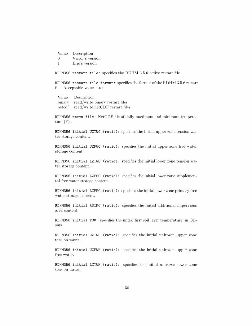
Value Description0 Victor’s version1 Eric’s version

RDHM356 restart file: specifies the RDHM 3.5.6 active restart file.

RDHM356 restart file format: specifies the format of the RDHM 3.5.6 restartfile. Acceptable values are:

Value Descriptionbinary read/write binary restart filesnetcdf read/write netCDF restart files

RDHM356 tmxmn file: NetCDF file of daily maximum and minimum tempera-ture (F).

RDHM356 initial UZTWC (ratio): specifies the initial upper zone tension wa-ter storage content.

RDHM356 initial UZFWC (ratio): specifies the initial upper zone free waterstorage content.

RDHM356 initial LZTWC (ratio): specifies the initial lower zone tension wa-ter storage content.

RDHM356 initial LZFSC (ratio): specifies the initial lower zone supplemen-tal free water storage content.

RDHM356 initial LZFPC (ratio): specifies the initial lower zone primary freewater storage content.

RDHM356 initial ADIMC (ratio): specifies the initial additional imperviousarea content.

RDHM356 initial TS0: specifies the initial first soil layer temperature, in Cel-sius.

RDHM356 initial UZTWH (ratio): specifies the initial unfrozen upper zonetension water.

RDHM356 initial UZFWH (ratio): specifies the initial unfrozen upper zonefree water.

RDHM356 initial LZTWH (ratio): specifies the initial unfrozen lower zonetension water.

150

RDHM356 initial LZFSH (ratio): specifies the initial unfrozen lower zonesupplemental free water.

RDHM356 initial LZFPH (ratio): specifies the initial unfrozen lower zone pri-mary free water.

RDHM356 initial SMC: specifies the initial volumetric content of total soil mois-ture for each layer.

RDHM356 initial SH2O: specifies the initial volumetric content of liquid soilmoisture for each layer.

RDHM356 initial WE: specifies the initial snow water equivalent without liquidwater, in mm.

RDHM356 initial LIQW: specifies the initial liquid water in snow.

RDHM356 initial NEGHS: specifies the initial negative snow heat, in mm.

RDHM356 initial TINDEX: specifies the initial antecedent temperature index.

RDHM356 initial ACCMAX: specifies the initial accumulated snow water tem-perature, including liquid, in Celsius.

RDHM356 initial SNDPT: specifies the initial snow depth, in cm.

RDHM356 initial SNTMP: specifies the initial average snow temperature.

RDHM356 initial SB: specifies the last highest snow water equivalent beforeany snow fall, in mm.

RDHM356 initial SBAESC: specifies the initial extent of snow cover during meltand new snow fall.

RDHM356 initial SBWS: specifies the initial snow water storage during meltand new snow fall, in mm.

RDHM356 initial STORAGE: specifies the initial snow liquid water attenuationstorage, in mm.

RDHM356 initial AEADJ: specifies the initial adjusted areal snow cover fraction[0, 1].

RDHM356 initial EXLAG: specifies the initial array of lagged liquid water val-ues.

151

RDHM356 initial NEXLAG: specifies the number of coordinates in the laggedliquid water array.

RDHM356 initial TA PREV: specifies the air temperature of previous timestep,in Celsius.

RDHM356 model timestep: "1hr"

RDHM356 restart output interval: "1hr"

RDHM356 TempHeight: 2.0

RDHM356 WindHeight: 10.0

RDHM356 DT_SAC_SNOW17: 3600

RDHM356 DT_FRZ: 1800

RDHM356 FRZ_VER_OPT: 1

RDHM356 SNOW17_OPT: 1

RDHM356 SACHTET_OPT: 1

RDHM356 NSTYP: 12

RDHM356 NVTYP: 14

RDHM356 NDINTW: 5

RDHM356 NDSINT: 5

RDHM356 NORMALIZE: 1

RDHM356 DSINTW: 0.05 0.25 0.60 0.75 1.00

RDHM356 DSINT: 0.05 0.25 0.60 0.75 1.00

RDHM356 PETADJ_MON: 1.0 1.0 1.0 1.0 1.0 1.0 1.0 1.0 1.0 1.0 1.0 1.0

RDHM356 CZIL: 0.12

RDHM356 FXEXP: 2.0

RDHM356 vegRCMAX: 5000

RDHM356 PC: -1

RDHM356 PET_OPT: -1

RDHM356 TOPT: 298

RDHM356 RDST: 1

RDHM356 thresholdRCMIN: 0.5

RDHM356 SFCREF: 4.0

RDHM356 BAREADJ: 0.230000004

RDHM356 SNOW17_SWITCH: 1

RDHM356 restart file: "none"

RDHM356 restart file format: "netcdf"

RDHM356 tmxmn file: "none"

RDHM356 initial UZTWC (ratio): 0.55

RDHM356 initial UZFWC (ratio): 0.14

RDHM356 initial LZTWC (ratio): 0.56

RDHM356 initial LZFSC (ratio): 0.11

RDHM356 initial LZFPC (ratio): 0.46

RDHM356 initial ADIMC (ratio): 1.0

RDHM356 initial TS0: 4.0

RDHM356 initial UZTWH (ratio): 0.1

152

RDHM356 initial UZFWH (ratio): 0.1

RDHM356 initial LZTWH (ratio): 0.1

RDHM356 initial LZFSH (ratio): 0.1

RDHM356 initial LZFPH (ratio): 0.1

RDHM356 initial SMC: 0.35 0.35 0.35 0.35 0.35 0.35

RDHM356 initial SH2O: 0.35 0.35 0.35 0.35 0.35 0.35

RDHM356 initial WE: 0

RDHM356 initial LIQW: 0

RDHM356 initial NEGHS: 0

RDHM356 initial TINDEX: 0

RDHM356 initial ACCMAX: 0

RDHM356 initial SNDPT: 0

RDHM356 initial SNTMP: 0

RDHM356 initial SB: 0

RDHM356 initial SBAESC: 0

RDHM356 initial SBWS: 0

RDHM356 initial STORAGE: 0

RDHM356 initial AEADJ: 0

RDHM356 initial EXLAG: 0 0 0 0 0 0 0

RDHM356 initial NEXLAG: 7

RDHM356 initial TA_PREV: 0

9.10 Irrigation

Irrigation scheme: specifies the name of the irrigation scheme to use. Ac-ceptable values are:

Value Descriptionnone No irrigation schemeSprinkler Demand sprinkler schemeFlood Demand flood scheme

Irrigation output interval: defines the output writing interval for irriga-tion.


Irrigation threshold: defines the irrigation trigger threshold for the floodand sprinkler irrigation schemes.

Sprinkler irrigation max root depth file: specifies the location of themax root depth file for sprinkler irrigation.

153

Flood irrigation max root depth file: specifies the

Drip irrigation max root depth file: specifies the location of the maxroot depth file for flood irrigation.

Irrigation scheme: "none"

Irrigation output interval: "1da"

Irrigation threshold: 0.50

Sprinkler irrigation max root depth file:

Flood irrigation max root depth file:

Drip irrigation max root depth file:

9.11 Routing

9.11.1 HYMAP routing

HYMAP routing model time step: specifies the timestep for the run.


HYMAP routing model output interval: defines the output writing intervalfor the HYMAP router.


HYMAP run in ensemble mode: specifies whether to run in ensemble mode.Acceptable values are:

Value Description0 Do not run in ensemble mode1 Run in ensemble mode

HYMAP routing method: specifies the HYMAP routing method to use. Ac-ceptable values are:

Value Descriptionkinematic use kinematic methoddiffusive use diffusive method

HYMAP routing model linear reservoir flag: specifies whether to use modellinear reservoir. Acceptable values are:

154

Value Description1 Use2 Do not use

HYMAP routing model evaporation option: specifies whether to computeevaporation in flood plains. Acceptable values are:

Value Description1 Compute evaporation in flood plains2 Do not compute evaporation in flood plains

HYMAP routing model start mode: specifies if a restart mode is being used.Acceptable values are:


HYMAP routing model restart interval: defines the restart writing intervalfor the HYMAP router.


HYMAP routing model restart file: specifies the HYMAP router active restartfile.

HYMAP routing LIS output directory: specifies the name of the top-leveloutput directory for HYMAP router. Acceptable values are any 40 characterstring.

HYMAP routing model time step:

HYMAP routing model output interval:

HYMAP run in ensemble mode:

HYMAP routing method:

HYMAP routing model linear reservoir flag:

HYMAP routing model evaporation option:

HYMAP routing model start mode:

HYMAP routing model restart interval:

HYMAP routing model restart file:

HYMAP routing LIS output directory:

155

9.11.2 NLDAS routing

NLDAS routing model output interval: defines the output writing intervalfor the NLDAS router.


NLDAS routing model restart interval: defines the restart writing intervalfor the NLDAS router.


NLDAS routing internal unit hydrograph file: specifies the internal unithydrograph file.

NLDAS routing transport unit hydrograph file: specifies the transportunit hydrograph file.

NLDAS routing coordinates order file: specifies the coordinates order file.

NLDAS routing initial condition for runoff: specifies the initial condi-tion for runoff file.

NLDAS routing initial condition for transport: specifies the initial con-dition for transport file.

NLDAS routing model start mode: specifies if a restart mode is being used.Acceptable values are:


NLDAS routing model restart file: specifies the NLDAS router active restartfile.

NLDAS routing model output interval:

NLDAS routing model restart interval:

NLDAS routing internal unit hydrograph file:

NLDAS routing transport unit hydrograph file:

NLDAS routing coordinates order file:

NLDAS routing initial condition for runoff:

NLDAS routing initial condition for transport:

NLDAS routing model start mode:

156

NLDAS routing model restart file:

9.12 Model output configuration

The output start time is used to define when to begin writing model output. Anyvalue not defined will default to the corresponding LIS start time. The outputstart time does not affect restart writing. Restart files are written according tothe LIS start time and the model restart output interval value.

The output start time is specified in the following format:

Variable Value DescriptionOutput start year: integer 2001 – present specifying output start yearOutput start month: integer 1 – 12 specifying output start monthOutput start day: integer 1 – 31 specifying output start dayOutput start hour: integer 0 – 23 specifying output start hourOutput start minutes: integer 0 – 59 specifying output start minuteOutput start seconds: integer 0 – 59 specifying output start second

Writing output may be restricted to a specified time with respect to any year.To restrict output to a specified time, you must set Output at specific time

only: to 1, and then you must specify the specific output writing time. If youchoose not to restrict output writing to a specified time, then you do not haveto set the specific output writing time variables.

Output at specific time only: specifies whether to write output only at aspecified time. Defaults to 0. Acceptable values are:

Value Description0 Do not restrict output to a specified time1 Restrict output to a specified time

The specific output writing time is specified in the following format:

Variable Value DescriptionSpecific output writing time (month): integer 1 – 12 specifying output monthSpecific output writing time (day): integer 1 – 31 specifying output daySpecific output writing time (hour): integer 0 – 23 specifying output hourSpecific output writing time (minute): integer 0 – 59 specifying output minuteSpecific output writing time (second): integer 0 – 59 specifying output second

Output start year:

Output start month:

157

Output start day:

Output start hour:

Output start minutes:

Output start seconds:

Output at specific time only:

Specific output writing time (month):

Specific output writing time (day):

Specific output writing time (hour):

Specific output writing time (minute):

Specific output writing time (second):

Model output attributes file: specifies the attributes to be used for a cus-tomizable model output. Please refer to the sample MODEL OUTPUT LIST.TBLfile for the complete specification.

Model output attributes file: ’./MODEL_OUTPUT_LIST.TBL’

9.13 Defining a time interval

Time interval values must be entered in a format where the timestep value isfollowed by 2 character string indicating the time units.

Examples include : 60ss, 30mn, 2hr, 0.5da

Acceptable values for the timestep units are:

Value Descriptionss secondsmn minuteshr hoursda daysmo monthsyr years

Units of months assumes a 30-day month.

Units of years assumes a 365-day year.

158

10 Specification of Input Forcing Variables

This section defines the specification of the input forcing variables for LIS. Thisfile is specified in a space delimited column format. Each row consists of thefollowing entries:

Short Name short name of the forcing variable.

Use option determines whether to include this the variable for use within LISAcceptable values are:

Value Description0 do not include the variable1 include the variable

Number of vertical levels The number of vertical levels corresponding tothe variable.

Units specified unit of the variable.

Note that this is a full list of input forcing variables. Not all models use allthese variables.

Note that being listed in the forcing variables.txt file does not guarantee that thefield will be available within LIS. Availablity depends on the support providedby the base forcing and supplemental forcing schemes selected in the lis.configrun-time configuration file.

#short name select vlevels units

Tair: 1 1 K # Near surface air temperature

Qair: 1 1 kg/kg # Near surface specific humidity

SWdown: 1 1 W/m2 # Incident shortwave radiation (total)

SWdirect: 0 1 W/m2 # Incident shortwave radiation (direct)

SWdiffuse: 0 1 W/m2 # Incident shortwave radiation (diffuse)

LWdown: 1 1 W/m2 # Incident longwave radiation

Wind_E: 1 1 W/m2 # Eastward wind

Wind_N: 1 1 m/s # Northward wind

Psurf: 1 1 Pa # Surface pressure

Rainf: 1 1 kg/m2s # Rainfall rate

Snowf: 0 1 kg/m2s # Snowfall rate

CRainf: 1 1 kg/m2s # Convective rainfall rate

Forc_Hgt: 0 1 m # Height of forcing variables

Ch: 0 1 - # Surface exchange coefficient for heat

Cm: 0 1 - # Surface exchange coefficient for momentum

159

Q2sat: 0 1 - # Saturated mixing ratio

Emiss: 0 1 - # Surface emissivity

Cosz: 0 1 - # Cosine of zenith angle

Albedo: 0 1 - # Surface albedo

PARDR: 0 1 - # Photosynthetically Active Direct Radiation

PARDF: 0 1 - # Photosynthetically Active Diffuse Radiation

SWnet: 0 1 - # Net Shortwave Radiation at the Surface

PET: 0 1 kg/m2s # Potential ET

RefET: 0 1 kg/m2s # Reference ET

CAPE: 0 1 J/kg # Convective Available Potential Energy

LPressure: 0 1 Pa # Level pressure

O3: 0 1 - # Ozone concentration

Xice: 0 1 - # Sea ice mask

QSFC: 0 1 kg/kg # Surface specific humidity

CHS2: 0 1 - # 2m Surface Exchange Coefficient for Heat

CQS2: 0 1 - # 2m Surface Exchange Coefficient for Moisture

T2: 0 1 K # 2m Air Temperature

Q2: 0 1 kg/kg # 2m Specific Humidity

TH2: 0 1 K # 2m Potential Temperature

TMN: 0 1 K # Soil Temperature at Lower Boundary

Snowflag: 0 1 - # Snowflag

Density: 0 1 kg/m3 # Atmospheric Density

VaporPress: 0 1 Pa # Vapor Pressure

VaporPressDeficit: 0 1 Pa # Vapor Pressure Deficit

Wind: 0 1 m/s # Wind Speed

160

11 Model Output Specifications

This section defines the specification of the model output from LIS. This file isspecified in a space delimited column format. Each row consists of the followingentries:

Short Name specifies the ALMA compliant short name of the variable.

Use option specifies whether to write the variable. Acceptable values are:

Value Description0 do not write the variable1 write the variable

Units: specifies the desired units of the output variable. You must check thesource code to determine all the units that are available for each output variable.

Sign Convention: specifies the direction in which the variable is consideredto have positive values. Note that the land models in LIS employ the ”tra-ditional approach” where all variables are considered positive in their domi-nant direction. i.e. precipitation and radiation are positive towards the surface(downward), evaporation, sensible heat and runoff are positive away from thesurface.


Value Description- No signUP DN Up or Down (Used for fluxes, Precip)IN OUT In or Out of the grid cell (Used for runoff, baseflow)INC DEC Increase or Decrease (Used for change in storager terms)S2L L2S Solid to Liquid and Liquid to Solid (for phase change terms)S2V V2S Solid to Vapor and Vapor to Solid (for phase change terms)E N Eastward and Northward (used for Wind components)

Time Average option determines how temporally process the variable. Ac-ceptable values are:

Value Description0 Instantaneous output1 Time averaged output2 Instantaneous and Time averaged output3 Accumulated output

Min/Max option determines whether to record minimum and maximum values

161

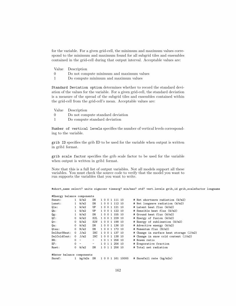
for the variable. For a given grid-cell, the minimum and maximum values corre-spond to the minimum and maximum found for all subgrid tiles and ensemblescontained in the grid-cell during that output interval. Acceptable values are:

Value Description0 Do not compute minimum and maximum values1 Do compute minimum and maximum values

Standard Deviation option determines whether to record the standard devi-ation of the values for the variable. For a given grid-cell, the standard deviationis a measure of the spread of the subgrid tiles and ensembles contained withinthe grid-cell from the grid-cell’s mean. Acceptable values are:

Value Description0 Do not compute standard deviation1 Do compute standard deviation

Number of vertical levels specifies the number of vertical levels correspond-ing to the variable.

grib ID specifies the grib ID to be used for the variable when output is writtenin grib1 format.

grib scale factor specifies the grib scale factor to be used for the variablewhen output is written in grib1 format.

Note that this is a full list of output variables. Not all models support all thesevariables. You must check the source code to verify that the model you want torun supports the variables that you want to write.

#short_name select? units signconv timeavg? min/max? std? vert.levels grib_id grib_scalefactor longname

#Energy balance components

Swnet: 1 W/m2 DN 1 0 0 1 111 10 # Net shortwave radiation (W/m2)

Lwnet: 1 W/m2 DN 1 0 0 1 112 10 # Net longwave radiation (W/m2)

Qle: 1 W/m2 UP 1 0 0 1 121 10 # Latent heat flux (W/m2)

Qh: 1 W/m2 UP 1 0 0 1 122 10 # Sensible heat flux (W/m2)

Qg: 1 W/m2 DN 1 0 0 1 155 10 # Ground heat flux (W/m2)

Qf: 0 W/m2 S2L 1 0 0 1 229 10 # Energy of fusion (W/m2)

Qv: 0 W/m2 S2V 1 0 0 1 198 10 # Energy of sublimation (W/m2)

Qa: 0 W/m2 DN 1 0 0 1 136 10 # Advective energy (W/m2)

Qtau: 0 N/m2 DN 1 0 0 1 172 10 # Momentum flux (N/m2)

DelSurfHeat: 0 J/m2 INC 1 0 0 1 137 10 # Change in surface heat storage (J/m2)

DelColdCont: 0 J/m2 INC 1 0 0 1 138 10 # Change in snow cold content (J/m2)

BR: 0 - - 1 0 1 1 256 10 # Bowen ratio

EF: 0 - - 1 0 1 1 256 10 # Evaporative fraction

Rnet: 0 W/m2 DN 1 0 1 1 256 10 # Total net radiation

#Water balance components

Snowf: 1 kg/m2s DN 1 0 0 1 161 10000 # Snowfall rate (kg/m2s)

162

Rainf: 1 kg/m2s DN 1 0 0 1 162 10000 # Rainfall rate (kg/m2s)

RainfConv: 1 kg/m2s DN 1 0 0 1 63 10000 # Convective rainfall rate (kg/m2s)

TotalPrecip: 1 kg/m2s DN 1 0 0 1 61 10000 # Total precipitation rate (kg/m2s)

Evap: 1 kg/m2s UP 1 0 0 1 57 10000 # Total evapotranspiration (kg/m2s)

Qs: 1 kg/m2s OUT 1 0 0 1 235 10000 # Surface runoff (kg/m2s)

Qrec: 0 kg/m2s IN 1 0 0 1 163 10000 # Recharge (kg/m2s)

Qsb: 1 kg/m2s OUT 1 0 0 1 234 10000 # Subsurface runoff (kg/m2s)

Qsm: 0 kg/m2s S2L 1 0 0 1 99 10000 # Snowmelt (kg/m2s)

Qfz: 0 kg/m2s L2S 1 0 0 1 130 10000 # Refreezing of water in the snowpack (kg/m2s)

Qst: 0 kg/m2s - 1 0 0 1 131 10000 # Snow throughfall (kg/m2s)

DelSoilMoist: 0 kg/m2 INC 1 0 0 1 132 10000 # Change in soil moisture (kg/m2)

DelSWE: 0 kg/m2 INC 1 0 0 1 133 1000 # Change in snow water equivalent (kg/m2)

DelSurfStor: 0 kg/m2 INC 1 0 0 1 134 1000 # Change in surface water storage (kg/m2)

DelIntercept: 0 kg/m2 INC 1 0 0 1 135 1000 # Change in interception storage (kg/m2)

RHMin: 0 - - 1 0 0 1 52 10 # Minimum 2-meter relative humidity (-)

Ch: 0 m/s - 1 0 0 1 208 10 # Surface exchange coefficient for heat

Cm: 0 m/s - 1 0 0 1 252 10 # Surface exchange coefficient for momentum

#Surface state variables

SnowT: 0 K - 1 0 0 1 165 10 # Snow surface temperature (K)

VegT: 0 K - 1 0 0 1 146 10 # Vegetation canopy temperature (K)

BareSoilT: 0 K - 1 0 0 1 147 10 # Temperature of bare soil (K)

AvgSurfT: 1 K - 1 0 0 1 148 10 # Average surface temperature (K)

RadT: 0 K - 1 0 0 1 149 10 # Surface radiative temperature (K)

Albedo: 1 - - 0 0 0 1 84 100 # Surface albedo (-)

SWE: 1 kg/m2 - 0 0 0 1 65 1000 # Snow Water Equivalent (kg/m2)

SWEVeg: 0 kg/m2 - 1 0 0 1 139 1000 # SWE intercepted by vegetation (kg/m2)

SurfStor: 0 kg/m2 - 1 0 0 1 150 1000 # Surface water storage (kg/m2)

#Subsurface state variables

SoilMoist: 1 kg/m2 - 0 0 0 4 86 1000 # Average layer soil moisture (kg/m2)

SoilTemp: 1 K - 0 0 0 4 85 1000 # Average layer soil temperature (K)

SmLiqFrac: 0 - - 0 0 0 4 160 100 # Average layer fraction of liquid moisture (-)

SmFrozFrac: 0 - - 0 0 0 4 140 100 # Average layer fraction of frozen moisture (-)

SoilWet: 0 - - 0 0 0 1 144 100 # Total soil wetness (-)

RelSMC: 0 m3/m3 - 0 0 0 4 141 1000 # Relative soil moisture

RootTemp: 0 K - 0 0 0 1 142 1000 # Rootzone temperature (K)

#Evaporation components

PotEvap: 0 kg/m2s UP 1 0 0 1 145 1 # Potential evapotranspiration (kg/m2s)

ECanop: 0 kg/m2s UP 1 0 0 1 200 1 # Interception evaporation (kg/m2s)

TVeg: 0 kg/m2s UP 1 0 0 1 210 1 # Vegetation transpiration (kg/m2s)

ESoil: 0 kg/m2s UP 1 0 0 1 199 1 # Bare soil evaporation (kg/m2s)

EWater: 0 kg/m2s UP 1 0 0 1 197 1 # Open water evaporation (kg/m2s)

RootMoist: 0 kg/m2 - 0 0 0 1 171 1 # Root zone soil moisture (kg/m2)

CanopInt: 0 kg/m2 - 0 0 0 1 223 1000 # Total canopy water storage (kg/m2)

EvapSnow: 0 kg/m2s - 1 0 0 1 173 1000 # Snow evaporation (kg/m2s)

SubSnow: 0 kg/m2s - 1 0 0 1 198 1000 # Snow sublimation (kg/m2s)

SubSurf: 0 kg/m2s - 1 0 0 1 143 1000 # Sublimation of the snow free area (kg/m2s)

ACond: 0 m/s - 1 0 0 1 179 100000 # Aerodynamic conductance

CCond: 0 m/s - 1 0 0 1 181 100000 # Canopy conductance

SoilET: 0 kg/m2 - 1 0 0 1 256 1 # Soil evaporation

AResist: 0 s/m - 1 0 0 1 256 1 # Aerodynamic resistance

#Other hydrologic variables

WaterTableD: 0 m - 0 0 0 1 174 1 # Water table depth (m)

TWS: 0 mm - 0 0 0 1 175 1 # Terrestrial water storage (mm)

163

GWS: 0 mm - 0 0 0 1 176 1 # Ground water storage (mm)

#Cold season processes

Snowcover: 0 - - 0 0 0 1 238 100 # Snow cover (-)

SAlbedo: 0 - - 0 0 0 1 184 1000 # Albedo of the snow-covered area (-)

SnowTProf: 0 K - 0 0 0 1 239 1000 # Temperature of the snow pack (K)

SnowDepth: 0 m - 0 0 0 1 66 1000 # Snow depth (m)

SLiqFrac: 0 - - 0 0 0 1 185 1000 # Fraction of SWE in the liquid phase

#Variables to compared against remote sensed data

LWup: 0 W/m2 UP 1 0 0 1 212 1 # Longwave radiation up from the surface (W/m2)

#Carbon variables

GPP: 0 kg/m2s2 DN 1 0 0 1 256 1 # Gross Primary Production

NPP: 0 kg/m2s2 DN 1 0 0 1 256 1 # Net Primary Production

NEE: 0 kg/m2s2 UP 1 0 0 1 256 1 # Net Ecosystem Exchange

AutoResp: 0 kg/m2s2 UP 1 0 0 1 256 1 # Autotrophic respiration

HeteroResp: 0 kg/m2s2 UP 1 0 0 1 256 1 # Heterotrophic respiration

LeafResp: 0 kg/m2s2 UP 1 0 0 1 256 1 # Leaf respiration

TotSoilCarb: 0 kg/m2 - 1 0 0 1 256 1 # Total soil carbon

TotLivBiom: 0 kg/m2 - 1 0 0 1 256 1 # Total living biomass

#Forcings

Wind_f: 1 m/s - 1 0 0 1 32 10 # Near surface wind (m/s)

Rainf_f: 1 kg/m2s DN 1 0 0 1 162 1000 # Average rainfall rate

Snowf_f: 0 kg/m2s DN 1 0 0 1 161 1000 # Average snowfall rate

CRainf_f: 1 kg/m2 DN 1 0 0 1 63 1000 # Average convective rainfall rate

Tair_f: 1 K - 1 0 0 1 11 10 # Near surface air temperature

Qair_f: 1 kg/kg - 1 0 0 1 51 1000 # Near surface specific humidity

Psurf_f: 1 Pa - 1 0 0 1 1 10 # Surface pressure

SWdown_f: 1 W/m2 DN 1 0 0 1 204 10 # Surface incident shortwave radiation

LWdown_f: 1 W/m2 DN 1 0 0 1 205 10 # Surface incident longwave radiation

PARDR_f: 0 W/m2 DN 1 0 0 1 256 10 # Surface incident PAR direct

PARDF_f: 0 W/m2 DN 1 0 0 1 256 10 # Surface incident PAR diffuse

#Additional forcings

DirectSW_f: 0 W/m2 - 1 0 0 1 166 10 # Surface direct incident shortwave radiation

DiffuseSW_f: 0 W/m2 - 1 0 0 1 167 10 # Surface diffuse incident shortwave radiation

NWind_f: 0 m/s N 1 0 0 1 34 10 # Northward wind

EWind_f: 0 m/s E 1 0 0 1 33 10 # Eastward wind

FHeight_f: 0 m - 1 0 0 1 256 10 # Height of forcing variables

Ch_f: 0 m/s - 1 0 0 1 208 10 # Surface exchange coefficient for heat

Cm_f: 0 m/s - 1 0 0 1 252 10 # Surface exchange coefficient for momentum

Emiss_f: 0 - - 1 0 0 1 256 10 # Surface emissivity

MixRatio_f: 0 kg/kg - 1 0 0 1 53 10 # Surface mixing ratio

CosZenith_f: 0 - - 1 0 0 1 256 10 # Cosine of zenith angle

Albedo_f: 0 - - 1 0 0 1 84 10 # Surface albedo

CAPE_f: 0 J/kg - 1 0 0 1 157 10 # Convective Available Potential Energy

Z0brd: 0 m - 1 0 0 1 256 1 # Z0brd

T2diag: 0 K - 1 0 0 1 256 1 # Diagnostic t2

Q2diag: 0 kg/kg - 1 0 0 1 256 1 # Diagnostic q2

Snowflag_f: 0 - - 1 0 0 1 256 1 # Snowflag

Density_f: 0 kg/m3 - 1 0 0 1 256 1 # Atmospheric density

VaporPress_f: 0 - - 1 0 0 1 256 1 # Vapor pressure

VaporPressDeficit_f: 0 - - 1 0 0 1 256 1 # Vapor pressure deficit

#Additional FEWSNET Forcings

164

PET_f: 0 kg/m2s - 0 0 0 1 228 1000 # Average PET rate

RefET_f: 0 kg/m2s - 0 0 0 1 256 1000 # Average RefET rate

TotalPrecip_f: 0 kg/m2 DN 0 0 0 1 256 1000 # Total precipitation

#Parameters

Landmask: 0 - - 0 0 0 1 81 1 # Land mask (0 - Water, 1 - Land)

Landcover: 0 - - 0 0 0 1 225 1 # Land cover

Soiltype: 0 - - 0 0 0 1 224 1 # Soil type

SandFrac: 0 - - 0 0 0 1 256 1 # Sand fraction

ClayFrac: 0 - - 0 0 0 1 256 1 # Clay fraction

SiltFrac: 0 - - 0 0 0 1 256 1 # Silt fraction

Porosity: 0 - - 0 0 0 1 240 1 # Porosity

Soilcolor: 0 - - 0 0 0 1 256 1 # Soil color

Elevation: 0 m - 0 0 0 1 196 10 # Elevation

Slope: 0 - - 0 0 0 1 222 10 # Slope

LAI: 0 - - 0 0 0 1 182 100 # LAI

SAI: 0 - - 0 0 0 1 256 100 # SAI

Snfralbedo: 0 - - 0 0 0 1 184 100 # Snow fraction albedo

Mxsnalbedo: 0 - - 0 0 0 1 159 100 # Maximum snow albedo

Greenness: 0 - - 0 0 0 1 87 100 # Greenness

Roughness: 0 m - 0 0 0 1 83 10 # Roughness

Tempbot: 0 K - 0 0 0 1 256 10 # Bottom soil temperature

#Routing

Streamflow: 0 m3/s - 1 0 0 1 256 10 # Streamflow

#VIC PET output

vic_pet_satsoil: 0 kg/m2s - 1 0 0 1 166 1 # Potential evap from saturated bare soil

vic_pet_h2osurf: 0 kg/m2s - 1 0 0 1 166 1 # Potential evap from open water

vic_pet_short: 0 kg/m2s - 1 0 0 1 166 1 # Potential evap (transpiration only) from short reference crop (grass)

vic_pet_tall: 0 kg/m2s - 1 0 0 1 166 1 # Potential evap (transpiration only) from tall reference crop (alfalfa)

vic_pet_natveg: 0 kg/m2s - 1 0 0 1 166 1 # Potential evap (transpiration only) from current vegetation and current canopy resistance

vic_pet_vegnocr: 0 kg/m2s - 1 0 0 1 166 1 # Potential evap (transpiration only) from current vegetation and 0 canopy resistance

#FLDAS-WRSI components

SOS: 0 - - 0 0 0 1 0 10 # Start-of-season [in dekads]

WRSI: 0 - - 0 0 0 1 0 10 # Water requirement satisfaction index [ratio]

KF2: 0 % - 0 0 0 1 0 10 # Percent of Season [%]

SumWR: 0 kg/m2 - 0 0 0 1 0 10 # Sum of Water Requirement [mm]

SumET: 0 kg/m2 - 0 0 0 1 0 10 # Sum of Evapotranspiration [mm]

SWI: 0 % - 0 0 0 1 0 10 # Soil Water Index [%]

SOSa: 0 - - 0 0 0 1 0 10 # Start-of-season Anomaly [in dekads]

TotalSurplusWater: 0 kg/m2 - 0 0 0 1 0 10 # Total surplus water [mm]

MaxSurplusWater: 0 kg/m2 - 0 0 0 1 0 10 # Max surplus water experienced in 1 dekad [mm]

TotalWaterDeficit: 0 kg/m2 - 0 0 0 1 0 10 # Total water deficit [mm]

MaxWaterDeficit: 0 kg/m2 - 0 0 0 1 0 10 # Max water deficit experienced in 1 dekad [mm]

TotalAETInitial: 0 kg/m2 - 0 0 0 1 0 10 # Actual evapotranspiration ~ Initial stage [mm]

TotalWRInitial: 0 kg/m2 - 0 0 0 1 0 10 # Water requirement ~ Initial stage [mm]

TotalSurplusWaterInitial: 0 kg/m2 - 0 0 0 1 0 10 # Surplus water ~ Initial stage [mm]

TotalWaterDeficitInitial: 0 kg/m2 - 0 0 0 1 0 10 # Water deficit ~ Initial stage [mm]

TotalAETVeg: 0 kg/m2 - 0 0 0 1 0 10 # Actual evapotranspiration ~ Vegetative stage [mm]

TotalWRVeg: 0 kg/m2 - 0 0 0 1 0 10 # Water requirement ~ Vegetative stage [mm]

TotalSurplusWaterVeg: 0 kg/m2 - 0 0 0 1 0 10 # Surplus water ~ Vegetative stage [mm]

TotalWaterDeficitVeg: 0 kg/m2 - 0 0 0 1 0 10 # Water deficit ~ Vegetative stage [mm]

TotalAETFlower: 0 kg/m2 - 0 0 0 1 0 10 # Actual evapotranspiration ~ Flowering stage [mm]

TotalWRFlower: 0 kg/m2 - 0 0 0 1 0 10 # Water requirement ~ Flowering stage [mm]

TotalSurplusWaterFlower: 0 kg/m2 - 0 0 0 1 0 10 # Surplus water ~ Flowering stage [mm]

165

TotalWaterDeficitFlower: 0 kg/m2 - 0 0 0 1 0 10 # Water deficit ~ Flowering stage [mm]

TotalAETRipe: 0 kg/m2 - 0 0 0 1 0 10 # Actual evapotranspiration ~ Ripening stage [mm]

TotalWRRipe: 0 kg/m2 - 0 0 0 1 0 10 # Water requirement ~ Ripening stage [mm]

TotalSurplusWaterRipe: 0 kg/m2 - 0 0 0 1 0 10 # Surplus water ~ Ripening stage [mm]

TotalWaterDeficitRipe: 0 kg/m2 - 0 0 0 1 0 10 # Water deficit ~ Ripening stage [mm]

PermWiltDate: 0 - - 0 0 0 1 0 10 # Permanent wilting date [dekad]

Wilting1: 0 - - 0 0 0 1 0 10 # First wilting date [dekad]

Wilting2: 0 - - 0 0 0 1 0 10 # Second wilting date [dekad]

WRSIa: 0 - - 0 0 0 1 0 10 # WRSI anomaly [-]

growing_season: 0 - - 0 0 0 1 0 10 # Growing season [season-year]

WHC: 0 kg/m2 - 0 0 0 1 0 10 # Water holding capacity; parameter [mm]

LGP: 0 - - 0 0 0 1 0 10 # Length of growing period; parameter [dekad]

WR_TimeStep: 0 kg/m2 - 0 0 0 1 0 10 # Water requirement per timestep(dekad) [mm]

AET_TimeStep: 0 kg/m2 - 0 0 0 1 0 10 # Actual ET per timestep [mm]

WRSI_TimeStep: 0 - - 0 0 0 1 0 10 # WRSI per timestep [-]

SurplusWater_TimeStep: 0 kg/m2 - 0 0 0 1 0 10 # Surplus water per timestep [mm]

#SacHTET specific output

sac_tsint: 0 K - 0 0 0 1 256 10 # Soil temperature of inteneded layer

sac_swint: 0 m3/m3 - 0 0 0 1 256 10 # Total volumetric soil moisture content of intended layer

sac_swhint: 0 m3/m3 - 0 0 0 1 256 10 # Liquid volumetric soil moisture content of intended layer

sac_frost: 0 - - 0 0 0 1 256 10 # Frost

sac_uztwc: 0 mm - 0 0 0 1 256 10 # UZTWC

sac_uzfwc: 0 mm - 0 0 0 1 256 10 # UZFWC

sac_lztwc: 0 mm - 0 0 0 1 256 10 # LZTWC

sac_lzfsc: 0 mm - 0 0 0 1 256 10 # LZFSC

sac_lzfpc: 0 mm - 0 0 0 1 256 10 # LZFPC

sac_adimpc: 0 mm - 0 0 0 1 256 10 # ADIMPC

sac_uztwh: 0 mm - 0 0 0 1 256 10 # UZTWH

sac_uzfwh: 0 mm - 0 0 0 1 256 10 # UZFWH

sac_lztwh: 0 mm - 0 0 0 1 256 10 # LZTWH

sac_lzfsh: 0 mm - 0 0 0 1 256 10 # LZFSH

sac_lzfph: 0 mm - 0 0 0 1 256 10 # LZFPH

#Snow17 specific output

snow17_swe: 0 kg/m2 - 0 0 0 1 256 10 # SWE

snow17_aeadj: 0 mm - 0 0 0 1 256 10 # AEADJ

snow17_neghs: 0 mm - 0 0 0 1 256 10 # NEGHS

snow17_liqw: 0 kg/m2 - 0 0 0 1 256 10 # LIQW

snow17_accmax: 0 mm - 0 0 0 1 256 10 # ACCMAX

snow17_rmlt: 0 kg/m2 - 0 0 0 1 256 10 # RMLT

Lake_Tsnow: 0 K - 0 0 0 1 256 10 # Lake temperature at the air snow interface

Lake_Tice: 0 K - 0 0 0 1 256 10 # Lake temperature at the snow snow interface

Lake_Tmnw: 0 K - 0 0 0 1 256 10 # Mean temperature of the water column

Lake_Twml: 0 K - 0 0 0 1 256 10 # Lake temperature of the mixed layer

Lake_Tbot: 0 K - 0 0 0 1 256 10 # Lake temperature at the water bottom

Lake_Tb1: 0 K - 0 0 0 1 256 10 # Temperature at the bottom of upper layer of sediments

Lake_CT: 0 - - 0 0 0 1 256 10 # Thermocline shape factor of lake

Lake_Hice: 0 - - 0 0 0 1 256 10 # Ice thickness above lake

Lake_Hml: 0 - - 0 0 0 1 256 10 # Thickness of mixed layer of lake

Lake_Hb1: 0 - - 0 0 0 1 256 10 # Thickness of upper layer of bottom sediments

Lake_Walbedo: 0 - - 0 0 0 1 256 10 # Water surface albedo over lake

Lake_IceAlbedo: 0 - - 0 0 0 1 256 10 # Ice surface albedo over lake

Lake_SnowAlbedo: 0 - - 0 0 0 1 256 10 # Snow surface albedo over lake

Lake_UFRa: 0 - - 0 0 0 1 256 10 # Lake friction velocity in air

Lake_UFRw: 0 - - 0 0 0 1 256 10 # Lake friction velocity in surface water

166

Lake_WConv: 0 - - 0 0 0 1 256 10 # Lake convective velocity scale

Lake_IW: 0 - - 0 0 0 1 256 10 # Lake radiation flux at the interface

Lake_Qbot: 0 - - 0 0 0 1 256 10 # Lake heat flux across water sediment boundary

RiverStor: 0 m3 - 0 0 0 1 256 10 # River water storage

RiverDepth: 0 m - 0 0 0 1 256 10 # River depth

RiverVelocity: 0 m/s - 0 0 0 1 256 10 # River flow velocity

FloodQ: 0 m3/s - 0 0 0 1 256 10 # Floodplain water discharge

FloodEvap: 0 m3 - 0 0 0 1 256 10 # Floodplain evaporation

FloodStor: 0 m3 - 0 0 0 1 256 10 # Floodplain water storage

FloodDepth: 0 m - 0 0 0 1 256 10 # Floodplain depth

FloodVelocity: 0 m/s - 0 0 0 1 256 10 # Floodplain flow velocity

FloodedFrac: 0 - - 0 0 0 1 256 10 # Flooded fraction

FloodedArea: 0 m2 - 0 0 0 1 256 10 # Flooded area

SurfElev: 0 m - 0 0 0 1 256 10 # Surface water elevation

RunoffStor: 0 m3 - 0 0 0 1 256 10 # Runoff reservoir storage

BaseflowStor: 0 m3 - 0 0 0 1 256 10 # Baseflow reservoir storage

RTM emissivity: 0 - - 0 0 0 1 256 10 # RTM emissivity

RTM Tb: 0 K - 0 0 0 1 256 10 # RTM brightness temperature

RTM SoilMoist: 0 m3/m3 - 0 0 0 1 256 10 # RTM soil moisture

Irrigated water: 0 kg/m2s - 0 0 0 1 256 10 # Irrigated water amount

167

12 User Support

This section describes how to request help from and provide feedback to the LISdevelopment team.

12.1 Modeling Guru

The NASA Center for Climate Simulation (NCCS) hosts a system called Model-ing Guru, https://modelingguru.nasa.gov. This system is a collection of forumsdiscussing many of NASA’s modelling efforts and related topics. LIS has a“community” within Modeling Guru.

This is system is open for reading, but registration is required to post questions.The front page of Modeling Guru provides information regarding requesting anaccount.

12.2 Requesting help

To request help from the LIS development team, please visit our communitywithin Modeling Guru at https://modelingguru.nasa.gov/community/atmospheric/lis.Select the “Discussions” tab. Please review the existing posts; your questionmay already be answered. If it is not, then please “Start a discussion” to postyour question there. Note that posting a question requires a registered account(see Section 12.1).

When reporting a bug or an error running LIS, please provide a description ofthe problem, including any error messages printed to the screen. Attach a copyof the lislog.0000 file. Also attach a copy of any relevant supporting files suchas the lis.config file, the MODEL OUTPUT LIST.TBL file, the ldt.config file,etc.

Please note that the LIS development team does not receive funding to providecommunity support. Your questions and issues are important to us, but we canaddress them only when time permits.

Please note that, due to U.S. federal law, we are not allowed to respond toanyone from a designated country. (See http://oiir.hq.nasa.gov/nasaecp/.) Bypolicy, we will not respond to messages from either non-institutional or non-organizational email addresses; e.g., we will not respond to email messages fromgmail.

168

https://modelingguru.nasa.gov

https://modelingguru.nasa.gov/community/atmospheric/lis

http://oiir.hq.nasa.gov/nasaecp/

A Frequently Asked Questions

This section provides a description of common error messages and a possiblefew options on how to address them.

1. Routine to diagnose error (variable)

Error:<var> field is not defined

for diagnostic output ..

Please exclude it from the model output attributes table

Program stopping..

This error occurs because the variable specified in the model output at-tributes file is not among the ones supported for output from the particularmodel. Either exclude the variable (turn it off) from the model outputattributes file or implement the routine within the model to support it.

2. Routine to diagnose error (units)

Error:<units> for field <var> is not defined


supported unit types: <list>

Program stopping..

This error occurs because the units of the variable specified in the modeloutput attributes file is not among the supported types. Either changethe incorrect unit specification or run the model simulation with a unittype that is supported by LIS.

3. Routine to diagnose error (direction)

Error:<direction> for field <var> is not defined


supported direction types: <list>

Program stopping..

This error occurs because the direction of the variable specified in themodel output attributes file is not among the supported types. Eitherchange the incorrect direction specification or run the model simulationwith a direction type that is supported by LIS.

169

B LIS Binary File Convention

(Draft, 4/23/2003)

B.1 Introduction

The majority of LIS data is saved in Fortran binary files, with various formats.This note defines the official LIS file scheme, to facilitate unified and consistentaccess to LIS data by LIS code, user programs and GDS client-server system.

B.2 Byte order

LIS data, by default, are saved in binary files as big endian numbers.

B.3 Storage organization

For a specific spatial resolution, the spatial grid space has NC columns and NRrows. In addition, a vectorized land space will often be used, with NL landpoints.

The minimum storage unit is a 2-D array of NC X NR, or a 1-D array of NLelements. Two dimensional grid space data and 1-D land space data are alwayssaved in separate files.

B.4 Missing/undefined values

Data type Missing/Undefined valuecharacter*1 CHAR(255)integer*1 -128integer*4 -9999 (?)real*4 (?)

170

B.5 File name extension convention and access code sam-ples

A LIS binary file name extention has 4 fields. The first field is one or morenumeric characters, indicating the total number of storage units the file has.The second field is the lower-case character “g” or “l”, indicating grid spaceor land space, respectively. The third field is the lower-case character “s” or“d”, indicating sequential or direct access. The last field, has 2 character width,with the first character indicating the number of bytes each number in the filetakes, and the second character, as “c”, “i”, or “r”, indicating the type of dataas character, integer or real, respectively.

Example1: datafile1.2gs4r

Sample Fortran code segment to read this file:

Real*4 v1(NC, NR), v2(NC, NR)

Open(12, file="datafile1.2gs4r", form="unformatted")

read(12)v1

read(12)v2

Close(12)

Example2: datafile2.15gd4i


Integer*4 v1(NC, NR), v10(NC, NR)

Open(12, file="datafile2.15gd4i", form="unformatted", &

access="direct", recl=NC*NR*4)

read(12, rec=1)v1

read(12, rec=10)v10

Close(12)

Example3: soilcolor.1ls1c


Character*1 color(NL)

Open(12, file="soilcolor.1ls1c", form="unformatted")

read(12)color

Close(12)

171

C CSIRO Open Source Software License Agree-ment (variation of the BSD / MIT License)

Copyright (c) 2015, Commonwealth Scientific and Industrial Research Organi-sation (CSIRO) ABN 41 687 119 230.

All rights reserved. CSIRO is willing to grant you a license to this Commu-nity Atmosphere Biosphere Land Exchange (CABLE) Software on the followingterms, except where otherwise indicated for third party material.

Redistribution and use of this software in source and binary forms, with orwithout modification, are permitted provided that the following conditions aremet:

• Redistributions of source code must retain the above copyright notice, thislist of conditions and the following disclaimer.

• Redistributions in binary form must reproduce the above copyright notice,this list of conditions and the following disclaimer in the documentationand/or other materials provided with the distribution.

• Neither the name of CSIRO nor the names of its contributors may be usedto endorse or promote products derived from this software without specificprior written permission of CSIRO.

EXCEPT AS EXPRESSLY STATED IN THIS AGREEMENT AND TO THEFULL EXTENT PERMITTED BY APPLICABLE LAW, THE SOFTWAREIS PROVIDED “AS-IS”. CSIRO MAKES NO REPRESENTATIONS, WAR-RANTIES OR CONDITIONS OF ANY KIND, EXPRESS OR IMPLIED, IN-CLUDING BUT NOT LIMITED TO ANY REPRESENTATIONS, WARRANTIESOR CONDITIONS REGARDING THE CONTENTS OR ACCURACY OFTHE SOFTWARE, OR OF TITLE, MERCHANTABILITY, FITNESS FORA PARTICULAR PURPOSE, NON-INFRINGEMENT, THE ABSENCE OFLATENT OR OTHER DEFECTS, OR THE PRESENCE OR ABSENCE OFERRORS, WHETHER OR NOT DISCOVERABLE.

TO THE FULL EXTENT PERMITTED BY APPLICABLE LAW, IN NOEVENT SHALL CSIRO BE LIABLE ON ANY LEGAL THEORY (INCLUD-ING, WITHOUT LIMITATION, IN AN ACTION FOR BREACH OF CON-TRACT, NEGLIGENCE OR OTHERWISE) FOR ANY CLAIM, LOSS, DAM-

172

AGES OR OTHER LIABILITY HOWSOEVER INCURRED. WITHOUT LIM-ITING THE SCOPE OF THE PREVIOUS SENTENCE THE EXCLUSION OFLIABILITY SHALL INCLUDE: LOSS OF PRODUCTION OR OPERATIONTIME, LOSS, DAMAGE OR CORRUPTION OF DATA OR RECORDS; ORLOSS OF ANTICIPATED SAVINGS, OPPORTUNITY, REVENUE, PROFITOR GOODWILL, OR OTHER ECONOMIC LOSS; OR ANY SPECIAL, IN-CIDENTAL, INDIRECT, CONSEQUENTIAL, PUNITIVE OR EXEMPLARYDAMAGES, ARISING OUT OF OR IN CONNECTION WITH THIS AGREE-MENT, ACCESS OF THE SOFTWARE OR ANY OTHER DEALINGS WITHTHE SOFTWARE, EVEN IF CSIRO HAS BEEN ADVISED OF THE POS-SIBILITY OF SUCH CLAIM, LOSS, DAMAGES OR OTHER LIABILITY.

APPLICABLE LEGISLATION SUCH AS THE AUSTRALIAN CONSUMERLAW MAY APPLY REPRESENTATIONS, WARRANTIES, OR CONDITIONS,OR IMPOSES OBLIGATIONS OR LIABILITY ON CSIRO THAT CANNOTBE EXCLUDED, RESTRICTED OR MODIFIED TO THE FULL EXTENTSET OUT IN THE EXPRESS TERMS OF THIS CLAUSE ABOVE “CON-SUMER GUARANTEES”. TO THE EXTENT THAT SUCH CONSUMERGUARANTEES CONTINUE TO APPLY, THEN TO THE FULL EXTENTPERMITTED BY THE APPLICABLE LEGISLATION, THE LIABILITY OFCSIRO UNDER THE RELEVANT CONSUMER GUARANTEE IS LIMITED(WHERE PERMITTED AT CSIRO’S OPTION) TO ONE OF FOLLOWINGREMEDIES OR SUBSTANTIALLY EQUIVALENT REMEDIES:

(a) THE REPLACEMENT OF THE SOFTWARE, THE SUPPLY OF EQUIV-ALENT SOFTWARE, OR SUPPLYING RELEVANT SERVICES AGAIN;

(b) THE REPAIR OF THE SOFTWARE;

(c) THE PAYMENT OF THE COST OF REPLACING THE SOFTWARE,OF ACQUIRING EQUIVALENT SOFTWARE, HAVING THE RELEVANTSERVICES SUPPLIED AGAIN, OR HAVING THE SOFTWARE REPAIRED.

IN THIS CLAUSE, CSIRO INCLUDES ANY THIRD PARTY AUTHOR OROWNER OF ANY PART OF THE SOFTWARE OR MATERIAL DISTRIBUTEDWITH IT. CSIRO MAY ENFORCE ANY RIGHTS ON BEHALF OF THERELEVANT THIRD PARTY.

173

Third Party Components

The following third party components are distributed with the Software. Youagree to comply with the license terms for these components as part of accessingthe Software. Other third party software may also be identified in separate filesdistributed with the Software.

Where parts of the CABLE code have not been written by CSIRO employees,permission to redistribute these code portions was granted under the CABLE li-cence v2.0 (http://www.cawcr.gov.au/projects/access/cable/cable licence agreement.pdf)and its predecessor.

Code contributors included:

G. Abramowitz, J. Exbrayat, K. Lu, J. Kala.

174

http://www.cawcr.gov.au/projects/access/cable/cable_licence_agreement.pdf

References

[1] A.A. Berg, J.S. Famiglietti, J.P. Walker, and P.R. Houser. Impact of biascorrection to reanalysis products on simulations of north american soil mois-ture and hydrological fluxes. Journal of Geophysical Research, 4490, 2003.

[2] W. Sawyer and A. da Silva. Protex: A sample fortran 90 source code docu-mentation system. Technical report, NASA GMAO, 1997. DAO Office Note97-11.

[3] J. Sheffield, G. Goteti, and E.F. Wood. Development of a 50-yr high-resolution global dataset of meteorological forcings for land surface modeling.Journal of Climate, 13:3088–3111, 2006.

175

Documents

LIS 7.1 Users’ Guide - NASA · 9.3.5 ANSA Snow Covered Fraction ... User’s Guide. This document de-scribes how to download and install the code and data needed to run the LIS