Liquidation Strategies in a Long-Short EquityPortfolio

Patrik Nilsson

Department of Mathematics,KTH, Stockholm,

October 2011

Abstract

Trading large volumes impact the price of the traded asset which implies a costwhen the position is liquidated. Because of this large investors, such as hedgefunds, need estimates of the expected market impact of their positions. I suggest amodel for the market impact of trading and use this model to analyze and comparedifferent liquidation strategies. I specifically consider liquidating large fractionsof a long-short equity portfolio. I consider two common liquidation strategies andcompare these to another strategy I introduce in this thesis; optimized liquidationwhich is the solution to an optimization problem. The results show that it is pos-sible to reduce expected market impact costs from liquidation while keeping theremaining portfolio within pre-specified risk limits.

iii

Acknowledgements

I want to thank my supervisor Filip Lindskog for guidance and support. I alsowant to thank Sam Nylander and Alexander Argiriou for their constant feedbackand for making my time a Brummer & Partners one of the most interesting and funparts of my studies at KTH.

v

Contents1 Introduction 1

1.1 Outline . . . . . . . . . . . . . . . . . . . . . . . . . . . . . . . . . 1

2 Definitions 32.1 General framework . . . . . . . . . . . . . . . . . . . . . . . . . . . 32.2 Risk measures . . . . . . . . . . . . . . . . . . . . . . . . . . . . . . 32.3 Net Exposure . . . . . . . . . . . . . . . . . . . . . . . . . . . . . . 32.4 Gross exposure . . . . . . . . . . . . . . . . . . . . . . . . . . . . . 42.5 Value-at-Risk . . . . . . . . . . . . . . . . . . . . . . . . . . . . . . 52.6 Beta . . . . . . . . . . . . . . . . . . . . . . . . . . . . . . . . . . . 62.7 Tracking Error . . . . . . . . . . . . . . . . . . . . . . . . . . . . . . 6

3 The market impact function 73.1 Differences between assets . . . . . . . . . . . . . . . . . . . . . . . 73.2 Empirical studies . . . . . . . . . . . . . . . . . . . . . . . . . . . . 9

3.2.1 Individual trades . . . . . . . . . . . . . . . . . . . . . . . . 93.2.2 Split orders . . . . . . . . . . . . . . . . . . . . . . . . . . . 103.2.3 Block trades . . . . . . . . . . . . . . . . . . . . . . . . . . 11

3.3 Why is the market impact function concave? . . . . . . . . . . . . . . 113.4 Time dependence . . . . . . . . . . . . . . . . . . . . . . . . . . . . 123.5 Other variables explaining market impact . . . . . . . . . . . . . . . 133.6 LOB modeling . . . . . . . . . . . . . . . . . . . . . . . . . . . . . 133.7 Modeling market impact . . . . . . . . . . . . . . . . . . . . . . . . 14

4 Transaction costs 164.1 Transaction costs due to market impact . . . . . . . . . . . . . . . . . 164.2 Square root market impact . . . . . . . . . . . . . . . . . . . . . . . 164.3 Indirect cost . . . . . . . . . . . . . . . . . . . . . . . . . . . . . . . 174.4 Total liquidation cost . . . . . . . . . . . . . . . . . . . . . . . . . . 18

5 The liquidation problem 195.1 Formalizing notation . . . . . . . . . . . . . . . . . . . . . . . . . . 195.2 The new spot price . . . . . . . . . . . . . . . . . . . . . . . . . . . 195.3 Cost of trading . . . . . . . . . . . . . . . . . . . . . . . . . . . . . 205.4 The NAV of the portfolio . . . . . . . . . . . . . . . . . . . . . . . . 205.5 Portfolio risk measures . . . . . . . . . . . . . . . . . . . . . . . . . 20

5.5.1 Net Exposure . . . . . . . . . . . . . . . . . . . . . . . . . . 205.5.2 Gross Exposure . . . . . . . . . . . . . . . . . . . . . . . . . 205.5.3 Value-at-Risk . . . . . . . . . . . . . . . . . . . . . . . . . . 21

5.6 Constraints on the weights to liquidate . . . . . . . . . . . . . . . . . 225.7 Different liquidation strategies . . . . . . . . . . . . . . . . . . . . . 22

vii

6 Case studies 246.1 A two stock portfolio . . . . . . . . . . . . . . . . . . . . . . . . . . 24

6.1.1 Total liquidation cost . . . . . . . . . . . . . . . . . . . . . . 246.1.2 Risk measures . . . . . . . . . . . . . . . . . . . . . . . . . 26

6.2 A four stock portfolio . . . . . . . . . . . . . . . . . . . . . . . . . . 306.2.1 The liquidation problem . . . . . . . . . . . . . . . . . . . . 31

6.3 Method . . . . . . . . . . . . . . . . . . . . . . . . . . . . . . . . . 32

7 Results 347.1 Total liquidation cost . . . . . . . . . . . . . . . . . . . . . . . . . . 347.2 Risk measures . . . . . . . . . . . . . . . . . . . . . . . . . . . . . . 347.3 Order of liquidation . . . . . . . . . . . . . . . . . . . . . . . . . . . 387.4 Tracking error . . . . . . . . . . . . . . . . . . . . . . . . . . . . . . 407.5 Beta . . . . . . . . . . . . . . . . . . . . . . . . . . . . . . . . . . . 43

8 Conclusion 458.1 Future work . . . . . . . . . . . . . . . . . . . . . . . . . . . . . . . 45

viii

1 IntroductionFinancial assets are similar to any other traded good in that prices are determined bysupply and demand. At any given price, there are only a limited number of potentialbuyers and sellers and thus a limited volume that can be traded at that price. If an in-vestor wants to buy (or sell) a larger volume he will only be able to trade a fraction ofthat volume at the original market price and as he proceeds to buy (or sell) the rest ofhis position he will have to accept less favorable prices in order to attract counterparties.

The way trading affects the price of the traded asset is often referred to as the marketimpact of trading. Market impact is generally not relevant for small investors. How-ever, for investors that trade in larger volumes market impact implies an additional costof trading and needs to be considered.

One of the larger investors in the market is the hedge fund industry. A hedge fundis a collective investment scheme that gets its capital from other investors, both privateinvestors and institutions. The aggregate capital allows the fund to invest aggressivelyin positions they consider profitable. Although buying and selling large positions al-ways require consideration about market impact, it is especially relevant when the fundfor some reason needs to liquidate a large fraction of its positions within a relativelyshort time frame. A typical example of this is when one of the fund’s large investorswithdraws his money. With a broad variety of investment strategies, deciding whichpositions to liquidate is not trivial. On one hand, the portfolio manager wants to sell themost liquid positions to avoid the cost of market impact. On the other hand, if only themost liquid positions are sold, then this will often change the properties of the portfolioin an unfavorable way for the remaining investors.

To balance these opposites, a portfolio manager needs to have a liquidation strategyready for when this situation arises. This is not only important from a managing pointof view. To keep and attract investors, a fund needs to be able to provide informationabout what costs investors will face when they withdraw their capital.

In this thesis I suggest a model for the market impact of trading and use this modelto compare different strategies for liquidating a large fraction of a portfolio. Specifi-cally, I consider long-short equity portfolios.

1.1 Outline• In Section 2 I introduce definitions relevant for this thesis.

• In Section 3 I suggest a model for the market impact of trading by presentingresults from a large number of empirical studies.

• In Section 4 I show what this model implies for the cost of trading.

• In Section 5 I formalize the liquidation problem that was briefly mentioned inthe introduction.

1

• In Section 6 I present two case studies where I implement the models that havebeen introduced.

• In Section 7 I present results.

• In Section 8 I conclude.

2

2 DefinitionsIn this section I define concepts that will be important in this thesis.

2.1 General frameworkThe investment universe available to a hedge fund is vast. I limit this universe byassuming the fund can only invest in stocks and in a money asset which is perfectlyliquid. The money asset is supposed to reflect any positions where the hedge fundstores capital rather than invest it. Typically, the risky positions in the portfolio areactive investment decisions whereas some capital is kept in assets whose expected re-turns are secondary to them being as liquid and risk free as possible. Because of this, Iassume the interest of the money asset is zero.

Consider a portfolio that have positions in n stocks. The number of shares held ineach stock is given by the weights

h(t) = (h1(t), h2(t), ..., hn(t))

The weights can be negative in which case they are called short positions (positiveweights are called long positions). The spot prices of the stocks are

S(t) = (S1(t), S2(t), ..., Sn(t))

The portfolio further consists of a position h0(t) in a perfectly liquid money asset S0(t)with zero interest rate, i.e. S0(t) = 1 for all t.

The mark-to-market value of this portfolio at time t is:

V (t) = h0(t) +

n∑i=1

hi(t)Si(t)

Furthermore, the net asset value (NAV) of the portfolio is equal to its mark-to-marketvalue. The NAV is an important concept that will be used frequently in this thesis.

2.2 Risk measuresAt Brummer & Partners, risk is calculated in the standard way in units of some cur-rency. However, it is often presented as a fraction of the NAV of the portfolio consid-ered. Below I will give formal definitions of the various risk measures to be used inthis thesis but in later sections I will discuss risk in relative rather than absolute terms.To emphasize this difference I include two simple examples below.

2.3 Net ExposureThe net exposure of an equity portfolio measures any long or short bias of the portfolio.It only includes the exposure of the stock positions, any risk free position is excluded.

3

Definition 1. Consider a portfolio Vp(t) consisting of the weights h (t) =(h1(t), ..., hn(t)

)in stocks with spot prices S (t) =

(S1(t), ..., Sn(t)

)and the weight h0(t) in the risk free

asset S0(t) = 1, ∀t. The net exposure of the portfolio is defined as

Net Exposure [Vp(t)] =

n∑i=1

hi(t)Si(t)

Example 1. Consider two stocks, S1(t) and S2(t), both with spot prices 100 SEK.Furthermore, consider a portfolio Vp(t) consisting of a short position of 100 sharesin S1(t), a long position of 200 shares in S2(t) and 10000 SEK in the risk free asseth0(t). The absolute net exposure of this portfolio is

Abs. Net Exposure [Vp(t)] =

n∑i=1

hi(t)Si(t) = −100 · 100 + 200 · 100 = 10000

The NAV of the portfolio is given by

V (t) = h0(t) +

n∑i=1

hi(t)Si(t) = 20000

The relative net exposure (relative the NAV) is given by

Rel. Net Exposure [Vp(t)] =

∑ni=1 hi(t)Si(t)

h0(t) +∑ni=1 hi(t)Si(t)

= 0.5

If the portfolio did not hold any capital in the risk free asset (i.e. h0(t) = 0), then theNAV would be equal to 10000 and relative net exposure of the portfolio would be

Rel. Net Exposure [Vp(t)] =

∑ni=1 hi(t)Si(t)

h0(t) +∑ni=1 hi(t)Si(t)

= 1

2.4 Gross exposureThe gross exposure is a measure of the leverage of the portfolio. It is defined in a waysimiliar to the net exposure.

Definition 2. Consider a portfolio Vp(t) consisting of the weights h (t) =(h1(t), ..., hn(t)

)in stocks with spot prices S (t) =

(S1(t), ..., Sn(t)

)and the weight h0(t) in the risk free

asset S0(t) = 1, ∀t. The gross exposure of the portfolio is defined as

Gross Exposure[Vp(t)] =

n∑i=1

|hi(t)|Si(t)

Example 2. Consider the same portfolio as in Example 1. The absolute gross exposureof this portfolio is

Abs. Gross Exposure [Vp(t)] =

n∑i=1

|hi(t)|Si(t) = 100 · 100 + 200 · 100 = 30000

4

The NAV of the portfolio is the same as in Example 1

V (t) = h0(t) +

n∑i=1

hi(t)Si(t) = 20000

The relative gross exposure (relative the NAV) is given by

Rel. Gross Exposure [Vp(t)] =

∑ni=1 |hi(t)|Si(t)

h0(t) +∑ni=1 hi(t)Si(t)

= 1.5

If the portfolio did not hold any capital in the risk free asset (i.e. h0(t) = 0), the NAVwould be equal to 10000 and the relative gross exposure of the portfolio would be

Rel. Gross Exposure [Vp(t)] =

∑ni=1 hi(t)Si(t)

h0(t) +∑ni=1 hi(t)Si(t)

= 3

2.5 Value-at-RiskValue-at-Risk is the value such that the probability of experiencing a loss larger thanthis value (over a given time horizon) is the given probability level. Many definitionsinclude a loss variable L defined as

L∆ = −(V (t+ ∆)− V (t)

)where ∆ is the time horizon of interest. Below is a (slightly modified) definition from[1].

Definition 3. Given some confidence level α ∈ (0, 1) and time horizon ∆, the Value-at-Risk of a portfolio Vp(t) at a confidence level α is given by the smallest number lsuch that the probability that the loss L exceeds l is not larger than (1 - α). Formally,

VaRα,∆ = infl ∈ R : P (L∆ > l) ≤ 1− α

There are a vast number of ways to estimate the VaR of a portfolio. A common ap-proach is to assume that the loss variable L∆ is normally distributed. This assumptiondoes not agree with empirical findings (the lack of heavy tails in the normal distributionunderestimates large price fluctuations). Nonetheless, this assumption is frequentlyused in the industry. The reason for this is that it is a reasonable approximation andthat it significantly simplifies computations. In practice, the Value-at-Risk of a positionwould be calculated in a number of different ways to address this problem. The normalassumption leads to a very simple expression for the Value-at-Risk which is presentedin the following corollary.

Corollary 1. If the loss variable L above is normally distributed, L ∈ N(µL, σ2L),

then the Value-at-Risk is given by

VaRα,∆ = µL + σLΦ(1− α)

where Φ is the standard normal cumulative distribution function.

Proof 1. The proof is left for the appendix.

5

2.6 BetaBeta is a measure of the relation between the log returns of a given asset (or portfolio)and the overall stock market. It can be described as a volatility adjusted correlation.In practice, beta is typically measured against a relevant index rather than against allexisting stocks.

Definition 4. Consider log returns Rp of a portfolio Vp(t) and log returns Rb of theoverall stock market (or possibly an index). The beta of the portfolio Vp is defined as

βp =Cov(Rp, Rb)

V ar(Rb)

2.7 Tracking ErrorTracking Error (TE) is a measure of how closely one portfolio “tracks” another portfo-lio. It is most often used as an ex post measure of the performance of some portfoliorelative a benchmark portfolio, such as an index. In that case it compares a series ofrealized returns over some time interval. In this thesis I will instead consider the lessused ex ante measure; the expected tracking error.

Definition 5. Consider a portfolio Vp(t) and a benchmark portfolio Vb(t) with (ran-dom) log returns Rp(∆) and Rb(∆) respectively over the time interval (t, t+ ∆). Fur-thermore, assume the marginal distribution functions of the stochastic variables Rp(∆)and Rb(∆) are fb(r) and fp(r) respectively. The expected tracking error of the portfolioVp(t) relative the portfolio Vb(t) is given by

TE =

√∫R

(fb(r)− fp(r)

)2dr

6

3 The market impact functionConsider a trader liquidating a large position during a relatively short time interval (sayhours or days). It can be argued that during this short time interval, the long term driftof the asset due to fundamentals only has a second order effect on price movements.Instead, the price movements are largely due to the change of supply and demand inthe market resulting from the large order. For notational clarity I assume, without lossof generality, that the trader starts liquidating his positions at time 0 and I propose thefollowing price process for the asset

S(t) = S(0)(

1 + εf(x(t); Ω) + ξ)

(1)

Here, S is the (mid) price of the asset a time t, ε denotes the sign of the trade (posi-tive for buy trades and negative for sell trades1) and f(x(t); Ω) is a (not yet specified)function describing the market impact of trading. The function depends on the volumex that has been transacted up until time t and also a set of other variables, for nowdenoted by Ω. With this notation it is obvious that the market impact function is di-mensionless. The last term, ξ is an error term with zero mean. It can be interpreted asreflecting the rest of the market activity during trading.

Trivially,E[S(t)

]= S(0)

(1 + εf(x(t); Ω)

)The intuitive way of deriving the market impact function is by performing statisticaltests on empirical data. However, this approach is problematic. To perform such astudy, detailed data about a significant number of large orders is needed. The fundsat Brummer & Partners refrain from trading very large orders exactly because of themarket impact that I intend to model. Fortunately, there exist a number of empiricalstudies where researchers have been given access to large data sets of large orders.In this thesis I will review a number of these studies and combine their results withintuition and theoretical arguments to derive a model for market impact.

3.1 Differences between assetsSpeaking of the market impact function is misleading. Different assets have com-pletely different properties and likely impact the market in different ways. Some assetsare standardized and traded on centralized exchanges whereas other assets are tradedoff-exchange in private agreements (often referred to as over-the-counter assets). Find-ing market impact functions for all different assets would obviously be preferable but

1It is intuitive that a large sell (buy) order will increase the supply (demand) of a stock in the marketand thus decrease (increase) prices. However, since every trade has a buy and a sell side it is not obviouswhat is meant by “sell orders” and “buy orders”. It is common practice to make the distinction based onwhich side that initiates the trade. The side that initiates the trade is called liquidity taker whereas the passiveside is called liquidity provider. Moro et al. [10] compares market impact between orders that are executedby liquidity takers and liquidity providers. They find that both strategies give a positive market impactbut impact is larger for the liquidity taker. The major difference between these two strategies is that onlyliquidity taking guarantees that the order is actually executed. Thus, large orders are typically executed bytaking liquidity.

7

the large number of assets makes this impossible.

This thesis will focus on the impact of trading stocks, which is the asset that has, byfar, been studied the most in academic papers. However, even for stocks there is notnecessarily a universal impact function. Stocks can be traded in different ways and thismight affect the impact of the trade.

The advances of computer technology during the last decade have allowed a signifi-cant growth of the electronic financial market. Today, most stock exchanges keep anelectronic trading platform where agents can trade in a limit order book (LOB). In aLOB any agent in the market is allowed to place limit orders that offer to buy (or sell)a certain number of shares of a stock at a maximum (or minimum) price. The highestbuy offer is called the best bid price and the lowest sell offer is called the best ask price.Any agent in the market is also allowed to place market orders that execute immedi-ately against the best price in the LOB. If the volume of the market order is larger thanthe volume offered at the best price, the remaining volume will execute against a lessfavorable price and this will lead to a price change of the stock. Agents placing limitorders are often referred to as liquidity providers whereas agents placing market ordersare referred to as liquidity takers.

If an order is small enough it can be executed in one transaction at the best price.However, the available volume at the best prices is typically small. A quick look at theNasdaq Nordic Stock Exchange shows that it is typically less than a percent of the dailyvolume for large cap stocks and a few percent of the daily volume for mid and smallcap stocks. To reduce market impact it has become common practice to split orders(even of modest sizes) and execute them incrementally over time.

Splitting orders introduces a time dependence on the impact of trading. Intuitively,if an order is executed slowly it allows liquidity providers to enter the market duringthe execution. This increases the supply (or demand) of the asset being bought (orsold). Thus, a more patient trading strategy is expected to decrease the impact of theorder. However, slow execution has a disadvantage. Holding the position over a longertime interval implies a larger market risk. Because of this, there is a tradeoff betweenthe expected cost of liquidation and the market risk of trading slowly.

Besides trading in the LOB, agents can also execute their positions outside the elec-tronic market in a privately negotiated transaction, often referred to as a block trade.This is typically done for very large orders but can also be done if the initiator of thetrade wants to avoid the market risk associated with order splitting.

There are obviously other ways stocks can be traded but this generalization capturesthe great majority of trades. Since stocks can be traded in different ways, empiricalstudies also differ in what they measure, the variables they consider and the resultsthey get. However, there is a consensus about the dependence on the traded volume.More or less all studies show that impact is a concave function of the traded volume.A concave function has a negative second derivative. The functions suggested in the

8

studies also have a positive first derivative. These two properties imply that the impactis an increasing function of the traded volume but that it increases slower and slower.This is true for individual orders, split orders and block trades. An example of such afunction is plotted in Figure 1. Some studies argue that market impact is a logarithmic

Figure 1: Graph of a concave function with positive first derivative

function but the majority propose a power law

f(x(t); Ω) ∼ x(t)ϕ (2)

with the notation introduced above. As mentioned x(t) is the volume executed up untiltime t. The function is concave if the exponent ϕ is between zero and one.

3.2 Empirical studiesThe majority of the studies about market impact considers individual trades, split ordersor block trades. In this section I will summarize some of the studies and fit the resultsto equation (2). As mentioned, all studies have different approaches to the subject andfitting all results to one equation is naturally an approximation.

3.2.1 Individual trades

Hausman, Lo and MacKinlay [3] consider six stocks from the New York and Ameri-can Stock Exchanges from January 4 to December 30 of 1988. The data set consists of

9

time-stamped trades, trade size and bid/ask quotes. They find a concave impact func-tion for all stocks but do not try to fit the results to a function.

Lillo, Farmer and Mantegna [4] used the Trade and Quote (TAQ) database to analyzeroughly 113 million transactions and 173 million quotes from the 1000 largest compa-nies on the New York Stock Exchange between 1995 and 1998. They find ϕ ≈ 0.5 forsmaller volumes and 0.2 for large volumes.

Farmer, Patelli and Zovko [5] use a data set from the London Stock Exchange be-tween August 1998 and April 2000, which includes a total of 434 trading days androughly six million events. They find ϕ ≈ 0.3.

Hopman [6] considers a data set from the Paris Bourse between January 1995 to Oc-tober 1999. The data set contains all the order submitted to the exchange and all thebest quotes available at any time. He considers 30 minute intervals and finds ϕ ≈ 0.4depending on the urgency of the order.

Potters and Bouchaud [7] refer to the study by Lillo, Farmer and Mantegna [4] andargue that the lower value of ϕ for larger volumes indicate that a logarithmic functionmight fit the impact function better. They analyse three stocks from the Paris Bourseand fit the results to a logarithmic function.

3.2.2 Split orders

The BARRA Market Impact model is considered somewhat of an industry standardand was derived by Torre and Ferrari [8]. They consider TAQ data from the NYSE,aggregate trades on a half hour time interval and find ϕ ≈ 0.5.

Gabaix et al. [9] have used TAQ data from the New York, London and Paris stockmarkets and found ϕ ≈ 0.5, although for relatively short time intervals (around 15minutes).

Moro et al. [10] considers transactions on the London Stock Exchange between Jan-uary 2002 and December 2004 as well as transactions on the Spanish Stock Exchangefrom January 2001 to December 2004. They find that ϕ ≈ 0.5 for the Spanish StockExchange and a slightly larger value for the London Stock Exchange.

Almgren et al. [11] use a data set consisting of almost 700,000 US stock trade or-ders executed by Citigroup Equity Trading desks. They consider almost 700,000 USstock trade orders executed by Citigroup Equity Trading desks and divide impact ina permanent part that changes as the order is executed and a temporary part that de-cays immediately after a transaction has been executed. The permanent part is to beinterpreted as the market impact of trading and the temporary part as representing fixedcosts and possibly any part of the impact that decays after the trade. For the temporarypart they find ϕ ≈ 0.6 and for the permanent part they find ϕ ≈ 0.9.

10

Engle, Ferstenberg and Russell [2] consider a sample of more than 200,000 ordersexecuted by Morgan Stanley and measure, not market impact, but transaction cost.They find transaction cost (relative the volume liquidated) increases approximately asa square root function of volume. Under the assumption that fixed costs (mainly thebid-ask spread) are linear in volume, this implies a square root market impact function.

3.2.3 Block trades

Block trades in the upstairs market have been studied by Keim and Madhavan [12].They use trading history from an investment management firm which contains tradedates, trade prices, number of shares traded and commissions paid for all block tradesin which the firm participated between 1985 and 1992. They find a concave dependenceon volume but do not try to fit the results to a function.

3.3 Why is the market impact function concave?There are a number of plausible explanations why market impact is concave. For indi-vidual trades, it has been suggested that the information of small trades hold approx-imately the same information as large trades. This implies that relative their volume,small trades impact the market more than large trades. Farmer et al. [14] suggestsconcavity is due to selective liquidity taking. This means that traders are more likely toplace large market orders when the available liquidity is favorable, implying that largevolumes do not have a smaller relative impact per se, but rather that large volumes areonly traded when they do not have a large impact.

Another explanation can be derived from the empirical finding that order flow2 is au-tocorrelated which was found independently by Lillo and Farmer [15] and Bouchaud[16]. The fact that order flow is autocorrelated implies that future order flow is pre-dictable and this raises an obvious question; if buying pushes prices up, selling pushesprices down and the sign of future orders are predictable, how do returns remain unpre-dictable? The return on a tic-by-tic scale is equal to the expected impact of buys andsells weighted with the respective probability of their occurrence. Farmer and Lillo ar-gue that impact is not fixed but depends on the markets predictions of the future orderflow. More specifically, a buy order followed by a series of buy orders must have asmaller impact (on average) for returns to remain unpredictable. It is suggested thatthis is caused by liquidity providers changing their quotes but it is emphasized that thisis only one possible explanation of many.

It should be pointed out that the market impact function is not concave for very smallvolumes. Any volume that can be executed against available liquidity at the best pricewill not have any impact on the spot price. Thus, the market impact function shouldbe slightly S-shaped. The majority of studies considered in this section argue that im-pact is concave even for very small volumes. The fact that the available liquidity atthe best prices is typically less than a percent of the daily volumes is an indication of

2The order flow refers to the series of signed trades in the market. The sign of a trade is positive if it isinitiated by the buyer and negative if it is initiated by the seller.

11

this. In the other end of the spectrum, for volumes corresponding to large fractions ofthe market capitalization of a company, it might be assumed that a concave functiondoes not model impact very well. However, such volumes imply responsibility for thestrategic decisions of the company and are more relevant for venture capitalists thanhedge funds.

3.4 Time dependenceIt is intuitive that the time taken to liquidate a position (often referred to as the tradingvelocity) affects market impact. Still, few papers have attempted to empirically fit thetime dependence to a function. As mentioned previously, trading over time introducesa dependence on the way trading is done. Is the trader liquidating her positions with aconstant trading velocity? Is she trying to match the available liquidity with her orders?Is she using some other strategy known only to herself? There are essentially endlessways in which a large order can be executed over a given time interval.

The majority of studies assume traders use a constant trading velocity. For instance,this is assumed in the study by Almgren et al. [11] previously introduced. They intro-duce a time dependence in their market impact model by assuming that impact shouldnot be measured as a function of the volume alone, but rather as a function of the frac-tion of the volume that is “normally” traded during the relevant time interval. Thus,they measure the dependence, not on volume, but on the variable

X

V T

where X is the traded volume, V is the daily volume and T is the time interval consid-ered. By introducing this variable they implicitly assume that trading over an n timeslonger time interval is equivalent to trading in an n times deeper market. The reasoningbehind this argument is fairly intuitive. However, the expression implies that tradingone days volume over one day has the same impact as trading a very small fraction ofthe daily volume during an equally small time interval. It is apparent that this expres-sion gives unreasonable results if used for very short time intervals.

In contrast, Engle, Ferstenberg and Russell [2] find only a weak dependence on tradingvelocity when measuring transaction costs in their extensive study.

Studies about price manipulation investigate specific trading strategies in more detail.The purpose is to investigate if models for market impact allow for price manipula-tion strategies with positive expected profits. A model introduced by Bouchaud et al.[16] and generalized by Gatheral [18] hypothizes that the impact of trading continu-ously reverts back to the pre-execution price level. In one way this is reasonable sinceit assumes trading only temporarily impacts the price from some fundamental value.However, it is difficult for the market to tell whether an order is executed because thetrader holds superior information about the company or simply because he wants to liq-uidate his position to raise cash. Furthermore, it is not unlikely that price manipulationstrategies with positive expected payoffs exist. The fact that there exist regulations in

12

this area is indicative that the strategies might be potentially profitable.

Seemingly, there is no consensus about how market impact depends on the tradingvelocity other than that a more rapid execution increases costs.

3.5 Other variables explaining market impactOther than the volume and the trading velocity, the most used variable is the volatil-ity. In the BARRA market impact model [8] Torre argues that higher volatility implieslarger market impact but he does not fit any functional form. Grinold and Kahn [19]introduce a model for transaction costs, seperate market impact from other costs andscale impact between stocks with the volatility. They state that their model fits nicelywith the trader rule of thumb that “it costs one day’s volatility to trade one day’s vol-ume”. Almgren et al. [11] argue that by trading a stock over time a trader participatesin the “normal” motion of the stock and that the volatility is a good proxy for this. Theydo not present statistical results but argue that volatility is the most important scalingvariable between stocks.

The bid-ask spread has an obvious effect on the transaction cost but not necessarilyon market impact. It is true that the spread tends to widen when markets becomeilliquid in crises but this effect is also captured in the volatility which also generallyincreases in stressed markets. Introducing a dependence on both the bid-ask spread andthe volatility might be superfluous.

There are also arguments for conditioning impact on the market captialization. Thisdependence is to some extent captured in the dependence on the daily volume but themarket capitalization also shows the hidden liquidity. Almgren [11] finds a weak de-pendence on the market capitalization, but with large error bars. Bikker et al. [20] findsthat the dependence on market capitalization pales in comparison to volatility.

3.6 LOB modelingI will briefly mention another approach from recent studies that are able to measureimpact more accurately than the studies considered so far. Instead of conditioningimpact on the volume traded, impact is conditioned on a microscopic variable; theorder flow imbalance. This variable is a measure of the imbalance between supplyand demand in the order book. Cont et al. [13] considers a data set consisting ofone calendar month (April, 2010) of trades and quotes (TAQ) data for 50 stocks andclaim that the order flow imbalance is able to explain impact to a far higher degree thanconditioning it on macroscopic variables. This is intuitive since microscopic variablesdescribe the actual structure of the limit order book at any time. However, from arisk management perspective there is a major disadvantage with using microscopicvariables. A condition for the model in this thesis is that it should be based on variablesthat are easily available and relatively easy to measure - this is generally not the casewith the order flow imbalance.

13

3.7 Modeling market impactThe previous section shows that there is overwhelming evidence that market impact isa concave function of the traded volume. The exact functional is unknown but empiri-cal studies indicate that it is a power law with an exponent close to 0.5. This is also inline with various transaction cost models that propose that market impact contributesto transaction costs as a square root function of the traded volume.

There is less consensus about the dependence on the trading velocity. Some mod-els have been proposed but they either give unreasonable results (Almgren), considermicroscopic variables (LOB modeling) or are to a large extent theoretical (price manip-ulation). The lack of robust empirical results concerning the time dependence meansthat including it in the model will significantly decrease the validity of the results.

I avoid this by considering a fixed time interval for the liquidation, thereby eliminatingthe time dependence from the model. This is not necessarily a significant limitation ofthe model. A reasonable assumption is that the volume determines the absolute impactof a trade and that the trading velocity only scales the impact. If the scaling is equal forall stocks this implies that deriving the optimal weights to liquidate for any time inter-val will give the optimal weights to liquidate for all time intervals. The time intervalchosen will only scale the total cost of the liquidation.

In the beginning of this section I introduced the following model for the stock priceas a function of the market impact of our trading.

S(t) = S(0)(1 + ε f

(x(t); Ω

)+ ξ(t)

)With the arguments and empirical results presented in the section above I propose thefollowing model for market impact.

f(x(t); Ω) = σd

√|x(t)|V

Here σd is the daily volatility, V is the daily volume and x(t) is the volume executedup until time t. Thus, market impact is a square-root function of the traded volume andit is scaled with the volatility and daily volume of the stock. A more volatile stock isexpected to have a larger market impact and a stock that is more frequently traded isexpected to have a smaller impact.

Introducing the market impact function in the model for the stock price gives

S(t) = S(0)(1 + ε σd

√|x(t)|V

+ ξ(t))

and trivially

E[S(t)

]= S(0)

(1 + ε σd

√|x(t)|V

)

14

Figure 2 shows the expected future spot price as a function of the number of dailyvolumes liquidated during the time interval (0, T ). The stock has a spot price of 100and a daily volatility of 1%.

Figure 2: The expected spot price of a stock at time T as a function of the number ofdaily volumes bought and sold during the time interval (0, T )

15

4 Transaction costsMost transaction cost models split costs up in different parts. Generally,

Transaction cost = Commission + Bid-ask spread + Market impact costs

The commission term reflects the fixed costs to be paid to a broker if trading is out-sourced. This term can be excluded if the portfolio manager places orders himself.The second term addresses the fact that a stock is never traded at the mid price, butrather at the best bid or best ask price. This thesis will disregard the first two termsand only focus on transaction costs coming from the market impact of our trading. Theargument for this is that commission and spread costs are linear in trade size and easilyadded to the cost resulting from market impact. Also, the market impact cost will tendto dominate for large orders.

4.1 Transaction costs due to market impactConsider liquidating a volume X (which can be negative) by splitting it up and exe-cuting it over the time interval t ∈ (0, T ). Let x(t) denote the volume that has beentransacted up until time t (where x(0) = 0 and x(T ) = X). At each infinitesimal timeinterval dt, the volume dx(t) will be executed at the spot price S(t). Thus, the cashraised from using a given liquidation strategy x(t) is

Cash raised =

∫ T

0

S(t) dx(t)

To be able to model this expression as an integral I assume that continuous trading ispossible. This is obviously practically impossible since it requires splitting orders ininfinite small parts. However, continuous trading is a good approximation if ordersare split up in many pieces. The obvious benchmark to compare this value with is thevalue of the position before the liquidation, i.e. X · S(0). I define the liquidation costas the difference between the mark-to-market value of the position before trading andthe cash that is actually raised from the liquidation.

Liq. cost = X · S(0)−∫ T

0

S(t) dx(t) =

∫ T

0

(S(0)− S(t)

)dx(t)

As mentioned, I only consider the market impact part of transaction costs. The liqui-dation cost, as defined here, is a part of this cost. However, as will be shown later inthis section, there is also an indirect cost related to market impact.

4.2 Square root market impactThe expression above is an ex post measure of the liquidation cost. The expectedliquidiation cost can be modeled by introducing a model for the stock price. I introduce

16

the market impact model derived in Section 3.

E[Liq. Cost] =

∫ T

0

(S(0)− E[S(t)]

)dx(t)

=

∫ T

0

(S(0)− S(0)(1 + εf(x(t)))

)dx(t)

=−∫ T

0

S(0) ε f(x(t)) dx(t)

=− ε

∫ T

0

S(0)σd

√|x(t)|V

dx(t)

=σdS(0)√

V

2

3|X|3/2

which is given in units of some currency. Notably, according to this model, the liquida-tion cost is independent of the liquidation strategy x(t). There are an infinite numberof ways to liquidate a given volume during a given time interval and different liquida-tion strategies likely imply different impact on the market. I assume, like many otherstudies, that the trader uses a constant trading velocity. This is in line with how tradingis actually done in practice3.

The derivation above shows that the absolute cost increases as a power law with expo-nent 3/2. However, the cost relative the value of the position liquidated (more specifi-cally its mark-to-market value when trading begins) is given by

1

|X| · S(0)

σdS(0)√V

2

3|X|3/2 ∼ |X|1/2

This is in line with the “square root” cost function suggested in literature [19], [21].

4.3 Indirect costThe situations considered so far have only focused on positions that are liquidatedcompletely. However, in many situations a portfolio manager will liquidate only afraction of a position. If trading impacts spot prices, this is going to change the mark-to-market value of the shares that remain in the portfolio after the liquidation. Morespecifically, consider holding a volume Y in an asset and then liquidating a smallervolumeX during the time interval t ∈ (0, T ). I define the indirect cost as the decreasedmark-to-market value of the remaining shares.

Indirect cost =(Y −X

)(S(0)− S(T )

)3Two common ex post benchmarks for the cash raised from a liquidation is the volume weighted average

price (VWAP) and the time weighted average price (TWAP). They are calculated at the end of the daywhen the exchange closes. A broker that executes an order on behalf of a customer can often guarantee thecustomer the VWAP or TWAP of his position. TWAP corresponds to a constant trading velocity (in time)and WVAP corresponds to matching the intradaily volume.

17

Introducing the market impact function derived in the previous section gives the ex-pected indirect cost as

E[Indirect cost] =(Y −X

)(S(0)− E[S(T )])

)=(Y −X

)(S(0)− S(0)

(1 + ε σd

√|x(t)|V

)))

=(Y −X

)S(0)

(− ε σd

√|x(t)|V

)The indirect cost can also be negative, which is equivalent to a profit. For example, amanager who holds a large volume in a stock can purchase further shares to increase themark-to-market value of his position. This is not surprising and there are examples ofthis happening in practice. As a matter of fact, this strategy is called price manipulationand is to some extent regulated. Secondly, this does not imply a profit in a strict sense.To actually realize the profit the manager will have to liquidate the positions, againimpacting the market. Still, this cost will be relevant for this thesis since hedge fundsuse spot prices to estimate the net asset value of their portfolios.

4.4 Total liquidation costThe total liquidation cost in this setting will be sum of the liquidation cost and theindirect cost.

E[Total liq. cost] =σdS(0)√

V

2

3|X|3/2 +

(Y −X

)S(0)

(− ε σd

√|x(t)|V

)This expression explains the decrease in the NAV of the portfolio from the liquidation.It is different from the market impact part of the general transaction cost model intro-duced in the beginning of this section. No previous model takes the indirect cost intoaccount when measuring transaction costs. The indirect cost is not really a cost, but itdoes decrease the NAV of the portfolio and I include it in the model.

18

5 The liquidation problemThe market impact framework can be extended to a portfolio setting. I will consider thesituation where a hedge fund considers liquidating a relatively large fraction of its posi-tions due to investor withdrawals. Since trading involves transaction costs the managerwould prefer to liquidate assets with little market impact or, even better, avoid tradingaltogether. However, liquidating only some of the positions will change the relativeweighting and overall properties of the remaining portfolio. Also, paying investorswithout liquidating any risky positions will generally increase the risk of the remainingportfolio. Thus, which liquidation strategy to use is not trivial.

5.1 Formalizing notationConsider a portfolio at time 0 (without loss of generalization) with the weights

h(0) = (h1(0), h2(0), ..., hn(0))

in stocks with spot prices

S(0) = (S1(0), S2(0), ..., Sn(0))

The portfolio also consists of a position h0(0) in a perfectly liquid money asset S0(0)with zero interest rate. I.e. S0(t) = 1 for all t.

Next, consider liquidating some fractions of the risky positions during the time intervalt ∈ (0, T ).

∆h(0) = (∆1h1(0),∆2h2(0), ...,∆nhn(0))

The domain of ∆i is

∆i ∈ [0, hi(0)] if hi(0) > 0

∆i ∈ [−hi(0), 0] if hi(0) < 0

I will motivate this below. At time T , the new weights in the risky positions are givenby

h(T ) =((h1(0)−∆1h1(0)), (h2(0)−∆2h2(0)), ..., (hn(0)−∆nhn(0))

)((1−∆1)h1(0), (1−∆2)h2(0), ..., (1−∆n)hn(0)

)In the following sections I summarize how withdrawals and a possible subsequent liq-uidation affect various properties of the portfolio.

5.2 The new spot priceThe expected spot price of stock i, at time T is given by

E[Si(T )

]= Si(0)(1 + ε σi

√|∆ihi(0)|

Vi), i ∈ 1, ..., n

19

5.3 Cost of tradingThe cost of trading was derived in the section above. With the notation introduced inthis section, the expected total liquidation cost is

E[Total liq. cost] =

n∑i=1

σiSi(0)√Vi

2

3|∆ihi(0)|3/2

+(hi(0)−∆ihi(0)

)S(0)

(− ε σi

√|∆ihi(0)|

Vi

)5.4 The NAV of the portfolioThe expected NAV of the portfolio immidiately after the liquidation is equal to theNAV before the liquidation less the total liquidation cost. I denote this V−(T ). At thispoint, a fraction k of the NAV will be paid out to investors. I denote the NAV of theremaining portfolio by V+(T ).

E[V−(T )] = V (0)− E[Total liq. cost]

andE[V+(T )] = (1− k) · E[V−(T )]

From the expression forE[V−(T )] it is apparent that the total liquidation cost is equva-lent to the decrease of the NAV of the portfolio due to the liquidation.

5.5 Portfolio risk measuresThe risk measures I will consider are net exposure, gross exposure and Value-at-Risk.

5.5.1 Net Exposure

The expected net exposure of the remaining portfolio is given by

Net Exposure =

∑ni=1 hi(T )E[Si(T )]

E[V+(T )]

=

∑ni=1(h1(0)−∆1h1(0))Si(0)(1 + ε σi

√|∆ihi(0)|

Vi)(

1− k)(V (0)− E[Total liq. cost]

)5.5.2 Gross Exposure

The expected gross exposure of the remaining portfolio is given by

Net Exposure =

∑ni=1 |hi(T )|E[Si(T )]

E[V+(T )]

=

∑ni=1 |h1(0)−∆1h1(0)|Si(0)(1 + ε σi

√|∆ihi(0)|

Vi)(

1− k)(V (0)− E[Total liq. cost]

)20

5.5.3 Value-at-Risk

I use the normal assumption to compute the (expected) Value-at-Risk of the remain-ing portfolio. The VaR will depend on the new spot prices and the new weights inthe portfolio. I assume that the covariance matrix of the stocks at time T is best esti-mated by the covariance matrix at time 0. Arguments can be made that the liquidationshould affect the volatilities and correlations of the stocks. However, I assume that thecovariance matrix captures the behavior of the stocks under normal market conditionsand that the liquidation only temporarily disrupts these conditions. With these assump-tions, the Value-at-Risk of the remaining portfolio, at a confidence level α and over thetime interval (T, T + ∆), is given by

V aRα,∆ =µL + Φ(1− α)σL

E[V+(T )]=

µL + Φ(1− α) · σL(1− k

)(V (0)− E[Total liq. cost]

)Here, µL and σL are the expected value and standard deviation of the loss variable Lintroduced in Section 2. To have use of this expression, the values of these two pa-rameters need to be computed. At this point it should be mentioned that it is commonpractice to disregard the expected value in the expression above. For short time inter-vals the expected value is typically small compared to the standard deviation. Anotherreason is that the expected value exhibits more seasonality than the volatility, it is lessrobust over time and more difficult to estimate.

It still remains to calculate the volatility of the loss variable L. Stock prices are typi-cally modeled as geometric stochastic processes. This implies the following expressionfor L∆

L∆ =−(V (T + ∆)− V (T )

)=−

( n∑i=1

hi(T )Si(T )eRi(∆) −n∑i=1

hi(T )Si(T ))

=−n∑i=1

hi(T )Si(T )(eRi(∆) − 1

)Here, Ri(∆) = Ri(T, T + ∆) is the log return of stock i over the interval (T, T +∆). For short time intervals, this expression can be approximated with a linearization.Noting that ex ≈ 1 + x for small x the following approximation can be made

L∆ =−n∑i=1

hi(T )Si(T )(eRi(∆) − 1

)≈−

n∑i=1

hi(T )Si(T )(1 +Ri(∆)− 1

)=−

n∑i=1

hi(T )Si(T )Ri(∆)

21

By assumtion, the returns Ri are normally distributed; Ri(∆) ∈ N(µi, σ2i ). The vari-

ance of the loss variable is given by

σ2L =Var[L∆]

= Var[−n∑i=1

hi(T )Si(T )Ri(∆)]

=

n∑i=1

n∑j=1

Cov(hi(T )Si(T )Ri(∆), hj(t)Sj(t)Rj(∆)

)=

n∑i=1

n∑j=1

hi(T )hj(T )Si(T )Sj(T )σiσjρi,j

Here ρi,j is the correlation coefficient between return Ri(∆) and Rj(∆). This is thevariance of the portfolio at time T . When we start the liquidation at time 0, the stockprices Si(T ) are stochastic and the expected variance is given by

V ar[L∆] =

n∑i=1

n∑j=1

hi(T )hj(T )E[Si(T )]E[Sj(T )]σiσjρi,j

The expected VaR of the portfolio at T is given by introducing the variance in theexpression for the VaR above (and excluding the expected value).

5.6 Constraints on the weights to liquidateI also impose restrictions on the weights that can be liquidated. More specifically, Ido not allow increasing the absolute volume in any stock, nor liquidating more thanthe volume we hold. The reason for this is, as mentioned, that this is equivalent toprice manipulation. Price manipulation is a vast area of its own and would make theinvestment universe significantly larger. It will also likely give extreme solutions sinceit would allow negative costs. Formally,

∆i ∈ [0, hi(0)] if hi(0) > 0

∆i ∈ [−hi(0), 0] if hi(0) < 0

5.7 Different liquidation strategiesChoosing which liquidation strategy to use is a balance between minimizing the costof trading and keeping the properties of the portfolio intact for the remaining investors.I will consider three approaches; the naive approach, proportional liquidation and op-timized liquidation.

The naive approach is to simply pay investors without liquidating any risky positions.The obvious advantage with this approach is that it does not involve any trading costs.

22

However, paying out money without liquidating any risky positions decreases the NAVof the portfolio without decreasing the market exposure. This increases the risk of theportfolio. If a withdrawal increases the risk of the portfolio for the remaining investors,this encourages investors to withdraw their money before anyone else. This is obvi-ously not a preferable consequence of a liquidation strategy.

Proportional liquidation, on the other hand, means the manager scales the portfoliodown by liquidating equal fractions of each position. This strategy has the advantagethat the properties of the remaining portfolio remain more or less unchanged4. The factthat these properties have been deliberately chosen by the (supposedly skilled) man-ager is further argument for a proportional liquidation strategy. However, this is stillnot necessarily the optimal liquidation approach. Firstly, proportional liquidation is notalways even possible; assets cannot be divided into arbitrarily small parts. Secondly, Iwill find that proportional liquidation is relatively expensive compared to other liquida-tion strategies. Thus, it can be argued that it is motivated to deviate from proportionalliquidation if this implies a lower expected cost.

How much to deviate from proportional liquidation depends on the preferences of theportfolio manager or the risk manager. By formulating an optimization problem withrelevant constraints it is possible to find solutions that imply smaller transaction costswithout changing the properties of the portfolio beyond some pre-specified limit. I de-fine optimized liquidation to be the result of this optimization problem. It is not obviouswhich constraints to use. From a risk manager point of view it is important that the re-maining portfolio satisfies all specified risk limits. For a portfolio manager, however,it is probably more important to keep a certain “profile” of the portfolio. This couldfor example mean that the portfolio should have a certain exposure to a specific asset,exposure to companies in a certain geographical area or that the portfolio manager isunwilling to liquidate certain positions that he considers profitable. However, it wouldbe difficult to generalize this in mathematical terminology. I will instead formulatethe constraints from a risk manager point of view. To address the portfolio manager’spoint of view, I will compare the tracking error of the remaining portfolio relative thepre-liquidation portfolio. This is a (somewhat crude) measure of how similar the twoportfolios are.

4Actually the cost of trading will change the properties of the portfolio. However, only slightly.

23

6 Case studiesTo illustrate the liquidation problem I consider two case studies. First, I form a toyportfolio consisting of two stocks that I use to show graphically how trading differentcombinations of the positions affect the properties of the remaining portfolio.

I also consider a portfolio consisting of four stocks from the Nasdaq Omx Nordic.They have been chosen to represent a portfolio that consists of some liquid and somemore illiquid stock positions. I use that portfolio to make a more thorough analysis ofthe problem.

6.1 A two stock portfolioConsider a portfolio consisting of two stocks and a cash postition. The stocks areweighted so that the portfolio is perfectly net neutral. The properties of the portfo-lio is given in Table 1. The risk measures are calculated as specified in Section 5.Furthermore, the covariance matrix Σ of the stocks daily log returns is given by

Stocks A Stock B CashSpot price 100 125 1Daily volume 1000 1250 –Weights -2500 2000 25000% of Gross 50 50 -% of NAV -100 100 100NAV 25000Net Exp. 0 %Gross Exp. 200 %Value-at-Risk 3.8 %

Table 1: Properties of two stock portfolio

Σ = 10−4 ·(

1.44 1.201.20 6.250

)This implies that the daily volatility of the stocks (the square root of the variances inthe covariance matrix) is 0.12 and 0.25 respectively.

6.1.1 Total liquidation cost

The cost of trading depends on the market impact function which scales with thevolatility and the daily volume. Since the stocks have otherwise similar propertiesStock B is expected to be more expensive to trade since it is more volatile. This is seenin Figure 3 which shows the cost of liquidation as a function of the number of sharesof Stock A and Stock B liquidated.

24

Figure 3: Cost of trading: The figure shows the total liquidation cost (relative the NAVof the pre-liquidation portfolio) as a function of the number of shares liquidated ofStock A and Stock B. Stock B has a higher volatility and is therefore more expensiveto liquidate.

One thing that is apparent from the figure is that it generally is cheaper to liquidateonly one of the positions rather than a combination of the two. This is because the con-cavity of the cost function implies a decreasing marginal cost. This can be illustratedgraphically. Assume a portfolio manager wants to decrease the gross exposure of hisportfolio by 50%. Figure 2 shows the cost of doing this for all linear combinations ofStock A and Stock B. I.e. the figure shows the cost of liquidating

αSA(0) + (1− α)SB(0) = 25000, α ∈ [0, 1]

The figure clearly shows that it is generally less expensive to only liquidate one posi-tion than to liquidate a combination of two positions. Notably, proportional liquidation(corresponding to the value 0.5 on the x-axis) is relatively expensive. The fact that itgenerally is less expensive to liquidate only one stock will become apparent in the nextcase study, where I solve an optimization problem.

25

Figure 4: Comparing liquidity cost: The figure shows the total liquidation cost (relativethe NAV of the pre-liquidation portfolio) of liquidating 50 percent of the mark-to-market value of the stock positions for all linear combinations of Stock A and Stock B.Notably, proportional liquidation (corresponding to 0.5 at horisontal axis) is relativelyexpensive.

6.1.2 Risk measures

I consider three risk measures, the Value-at-Risk, the net exposure and the gross ex-posure. Figure 5 shows the Value-At-Risk of the portfolio after we liquidate a givenfraction of our stock positions. The VaR also depends on the fraction of the NAV that ispaid out to investors after the liquidation. In this figure, I consider the situation wherethis amount is zero. If some fraction is paid out, the VaR-surface would have the sameshape, only scaled.

26

Figure 5: Value-at-Risk: The figure shows the VaR of the remaining portfolio whena given fraction of Stock A and Stock B is liquidated. Liquidating only Stock B willdecrease the VaR since the remaining portfolio is then left with a higher relative weightin Stock A, which is less volatile.

The figure shows that if all shares are sold, then the VaR becomes zero since we donot have any risky positions left. Figure 6 shows the same graph from another angle.

27

Figure 6: Value-at-Risk: This is the same figure as Figure 4, only from a differentangle.

Figure 7 and Figure 8 show the net and gross exposure of the remaining portfolio.Again, I consider the situation where no fraction of the NAV is paid out to investorsafter the liquidation.

28

Figure 7: Net Exposure: The figure shows the net exposure of the remaining portfoliowhen a given fraction of Stock A and Stock B is liquidated. Liquidating Stock A willleave the remaining portfolio net positive since the portfolio holds a short position inStock A

29

Figure 8: Gross Exposure: The figure shows the gross exposure of the remaining port-folio when a given fraction of Stock A and Stock B is liquidated. Liquidating shares inany stock will decrease the gross exposure.

The figures in this section illustrate the properties of the problem that is to besolved. Figure 3 and Figure 4 show that the cost of liquidating only one stock is gener-ally less expensive than to liquidate a combination of two stocks with the same mark-to-market value. However, Figures 6-8 show that liquidating shares in only one of thestocks increases the risk more than liquidating a combination of two stocks. Thus, thefigures illustrate the balance that has to be made between reducing the market impactcost of trading and managing the risk of the remaining portfolio. This problem will bediscussed in more detail in the following section, where I consider a portfolio of fourstocks.

6.2 A four stock portfolioI consider four stocks from Nasdaq Omx Nordic; H&M, Danske Bank, Eniro and DSV.I use data from 2011-02-01 to 2011-08-20 to estimate the daily volume, volatility andcovariance matrix of the stocks. I estimate the daily volume with a 30 day average.The properties of the stocks and the portfolio is given in Table 2.

The portfolio is approximately net neutral with a leverage slightly above two. Thestocks are supposed to represent an equity portfolio consisting of a mix of stocks thatare traded more and less frequently and have different volatilities. The covariance ma-

30

H&M Danske Bank Eniro DSV CashSpot price 188 77.0 16.7 100 1Daily Volatility 1.54% 2.33% 3.33% 1.70% 0Daily Volume 5.3 M 2.3 M 0.9 M 1.2 M -

Portfolio propertiesWeights (in million shares) 3 -5 4.25 -2.5 6 · 108

Weights (in daily vol.) 0.566 -2.17 4.72 -2.08 -Exposure (percent of gross) 44.4 30.3 5.60 19.70 -Exposure (percent of NAV) 94.0 -64.2 11.8 -41.7 100NAV (of portfolio) 6.0 · 108

Risk measures (percent of NAV)Net Exposure 0 %Gross Exposure 217 %Value-at-Risk 3.29 %

Table 2: Properties of the four stock portfolio

trix of the one day log returns of the stocks is given by

Σ = 10−4 ·

2.39 0.85 1.30 0.890.85 5.43 2.84 1.991.30 2.84 11.1 2.100.89 1.99 2.10 2.87

6.2.1 The liquidation problem

I summarize the liquidation problem that has been discussed throughout the thesis.There are a number of properties that are preferable for a liquidation strategy.

1. The total liquidation cost should be as small as possible. This cost is equal to thedecrease in the NAV of the portfolio.

2. From a risk manager point of view, the risk of the remaining portfolio must notexceed any pre-specified risk limits.

3. From a portfolio manager point of view, the remaining portfolio should have aprofile similar to the original portfolio.

The properties are to some extent incompatible and the problem can be formalizedas an optimization problem. I will consider the total liquidation cost as the objectivefunction to minimize and take the risk manager point of view and introduce variousrisk measures as constraints. To address the portfolio manager, I will analyze the resultby comparing the tracking error of the portfolio before and after the liquidation. The

31

resulting optimization problem can be expressed, heuristically

minimize expected total liquidation costs.t. Value-at-Risk ≤ pre-specified limit

Gross exposure ≤ pre-specified limitNet Exposure ≤ pre-specified limit

Weights liquidated ∈ Allowed domain

The objective function to minimize is intuitive since the total liquidation cost (as de-fined) is equal to the expected decrease in the NAV of the portfolio from the liquidation.Since investors are paid after the NAV of the portfolio has been re-estimated, this costaffects both investors withdrawing their capital and the investors that remain.

The objective function and risk measures have been explicitly expressed in Section5. For this case study I will use the following risk limits (all relative the NAV of theportfolio).

• Value-at-Risk: 4 %

• Net exposure: +/- 50 %

• Gross exposure: 250 %

Furthermore, I will consider the liquidation over a time interval of one day, i.e. T = 1.As mentioned in Section 3.7 it is necessary to consider a fixed time interval since thereare no robust results regarding the time dependence of market impact. The reasonthe time interval chosen is one day is because that, at Brummer & Partners, that timeinterval is representative of the time intervals over which large orders are typicallyliquidated.

6.3 MethodThe optimization problem is highly non-linear; both the objective function and theconstraints. There are a number of different algorithms that can be used to solve op-timization problems of this type. I have used sequential quadratic programming (SQP).

SQP is one of the most effective methods for solving non-linear constrained opti-mization problems [22]. It is an iterative algorithm which solves, at each iteration,a quadratic programming problem. I have used the SQP-algorithm that is implementedin the software MATLAB. In the results section I plot the cost function and variousconstraints as a function of the fraction of the NAV that is to be paid out to investors.Because of this, I have solved the optimization problem for a large number of suchvalues.

The optimization problem has several local minima which makes the outcome from

32

the algorithm highly dependent on the first guess. Because of this, a lot of time hasbeen spent trying different start guesses and comparing results. Fortunately, the lo-cal minima are not found arbitrarily in the feasible region. The minima are typicallyfound when one stock is liquidated to the largest possible extent and one (or more)other stock is liquidated further just so that the result satisfies the risk constraints. Tofind the global minima I used start guesses for different combinations of stocks thathave this property, and compared the results. I also used random start guesses to findlocal minima that do not have this property in the unlikely event that any of these localminima are actually the global minimum (which they were not).

The difficulty in finding the global minimum will lead to problems when generaliz-ing this framework to a real portfolio that typically consists of a significantly largernumber of positions. However, it is not necessarily of outmost importance to find theglobal minimum for problems of this type. A portfolio manager will likely be satisfiedif he can find any reasonable liquidation strategy that has a significantly lower expectedcost than some other strategy he considers.

33

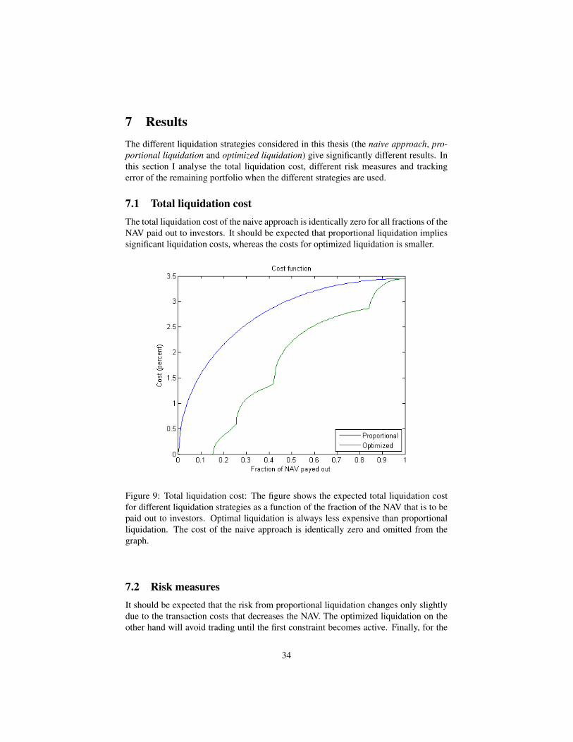
7 ResultsThe different liquidation strategies considered in this thesis (the naive approach, pro-portional liquidation and optimized liquidation) give significantly different results. Inthis section I analyse the total liquidation cost, different risk measures and trackingerror of the remaining portfolio when the different strategies are used.

7.1 Total liquidation costThe total liquidation cost of the naive approach is identically zero for all fractions of theNAV paid out to investors. It should be expected that proportional liquidation impliessignificant liquidation costs, whereas the costs for optimized liquidation is smaller.

Figure 9: Total liquidation cost: The figure shows the expected total liquidation costfor different liquidation strategies as a function of the fraction of the NAV that is to bepaid out to investors. Optimal liquidation is always less expensive than proportionalliquidation. The cost of the naive approach is identically zero and omitted from thegraph.

7.2 Risk measuresIt should be expected that the risk from proportional liquidation changes only slightlydue to the transaction costs that decreases the NAV. The optimized liquidation on theother hand will avoid trading until the first constraint becomes active. Finally, for the

34

naive approach, risk will increase out of control as the NAV is decreased while themarket exposure remains unchanged. The only risk measure that is left unchanged isthe net exposure. This is because the absolute net exposure is always zero. However,only a slight deviation from zero of the absolute net exposure will lead to a significantrelative net exposure. The plots of the risk measures can help explain the shape of theoptimized cost in Figure 9. The general tendency of the optimization algorithm is toliquidate shares in only one stock to the furthest possible extent. At some point, a riskconstraint becomes active and the algorithm will find that it needs to liquidate sharesin another stock to satisfy the constraints. After presenting plots of the risk measures Iwill summarize which contraints that are active for each fraction of the NAV and whatthis implies for the optimized liquidation strategy.

35

Figure 10: Value-at-Risk: The figure shows the expected VaR of the remaining port-folio as a function of the fraction of the NAV that is to be paid out to investors. Pro-portional liquidation implies only a slight increase in the VaR, coming from the factthat transaction costs will decrease the NAV. Optimal liquidation will never increasethe VaR above the prespecified limit of 4 per cent. The naive approach of not trading atall will imply increasing risk as money is being paid out from the NAV. The risk fromthis approach is asymptotically infinite.

36

Figure 11: Net Exposure: The figure shows the expected Net Exposure of the remainingportfolio. The expected net exposure of the naive approach is zero since the expectedabsolute risk exposure is zero. However, the portfolio is highly leveraged and a smalldeviation in any of the stock prices will lead to a significant net exposure of the port-folio. The expected net exposure of the proportional liquidation is slightly non-zerodue to the difference in impact of the different stocks. The behavior of the optimizedliquidation will be discussed in the next section.

37

Figure 12: Gross Exposure: The figure shows the expected Gross Exposure of theremaining portfolio. The figure will be discussed in more detail in the following section

7.3 Order of liquidationFigure 13 shows the fractions of each stock position that is liquidated, as a function ofthe NAV to be paid out to investors. This figure can be used, together with the figuresshowing the risk measures, to analyze what the optimization algorithm suggests foreach fraction of the NAV.

For small volumes, no risk constraint is active and the algorithm suggests simply pay-ing investors cash without liquidating any of the stock positions. For a fraction ofthe NAV of about 15 %, the gross exposure constraint becomes active. At this pointthe algorithm suggests liquidating H&M which is the stock with the smallest expectedmarket impact.

The next constraint that becomes active is the Value-at-Risk at about 22 %. At thispoint there are two ways to go; either liquidating a small volume in another stockor keep liquidating H&M. However, in order to liquidate more shares in H&M it isnecessary to liquidate disproportionally larger volumes in order to reduce the marketexposure relative the NAV. Simply put, in order to be able to pay out an additional 100SEK, it might be necessary to liquidate stock positions worth 150 SEK to keep the riskconstraints satisfied. If another stock is liquidated, the latter sum might only be 125

38

SEK but that might still imply a larger cost due to market impact. Indeed, the algorithmsuggests liquidating H&M further and the increasing derivative of H&M in the graphat this point indicates that it really is liquidated disproportionally (as suggested).

At about 25 % the net exposure constraint becomes active. At this point, it is necessaryto liquidate a short position to keep this constraint satisfied. The algorithm suggestsliquidating DSV which has the lowest marginal expected total liquidation cost of theshort positions.

At about 30 % the algorithm suggests changing strategy drastically. It finds that itis less expensive to liquidate all of DSV than to keep liquidating in a similar manner.This result is to some extent expected since this strategy allows liquidating a smallerabsolute volume and still satisfy the Value-at-Risk constraint. After this, the suggestedstrategies are rather predictable. The concavity of market impact implies a decreas-ing marginal (expected) total liquidation cost. Because of this, the algorithm suggestsliquidating shares in as few stocks as possible. Thus, the stocks with larger expectedmarket impact (specifically Eniro) will not be considered for anything but for very largefractions of the NAV.

The analysis shows that the concavity of market impact (combined with the constraints)can lead to some extreme results. Notably, for about 25 % of the NAV, the algorithmsuggests not liquidating any fraction of DSV. However, for about 30 % it suggests liq-uidating the DSV position completely. Considering the relatively non-robust model formarket impact this is naturally an undesirable property. Nonetheless, the differencebetween the value of the objective function at different local minima is typically rathersmall. Both values are also significantly better than that of the benchmark strategy(proportional liquidation). Thus, the optimization shows that it is possible to signifi-cantly reduce the expected total liquidation cost by considering liquidation strategiesdifferent from proportional liquidation.

39

Figure 13: Order of liquidation: The figure shows the fraction of each stock positionthat the optimization algorithm suggests should be liquidated. It is plotted as a functionof the fraction of the NAV that is to be paid out to investors.

7.4 Tracking errorIn the case study above, a portfolio V (0) at time 0 is, to some extent, liquidated duringthe time interval (0, T ) so that the new portfolio V (T ) has potentially very differentproperties. More specifically, any change in prices of the stocks and weighting in theportfolio will change the distribution of the (log) return of the portfolio.

At time T , the future return of the portfolio can be modeled as

V (T + ∆) = V (T )eRV (∆)

where RV (∆) is the log return of the portfolio during the time interval (T, T + ∆).In the case study above I have considered performing the liquidation during one dayso that T = 1. Furthermore, at time T I consider the distribution of the portfolio overthe next day so that ∆ = 1. However, in the derivation below I will use T and ∆ fornotational clarity.

40

An explicit expression for this stochastic variable is given by

RV (∆) = ln(V (T + ∆)

V (T )

)= ln

(h0(T ) +∑ni=1 hi(T )Si(T )eRi(∆)

h0(T ) +∑ni=1 hi(T )Si(T )

)where Ri(∆) is the log return of stock i. The expected stock prices Si(T ) and portfo-lio weights hi(T ) naturally depend on the specific liquidation strategy used during thetime interval (0, T ).

Since the relative weighting (and thus distribution) of the pre-liquidation portfolio hasbeen deliberately chosen by the portfolio manager, it is interesting to compare thatdistribution to that of the post-liquidation portfolio. More specifically, I consider twoscenarios.

Scenario 1 (benchmark scenario): I consider the situation where no investors with-draw any money, no money is paid out and the portfolio weights remain unchanged. Inthis scenario no liquidation is performed and the changes in stock prices are only dueto “normal” market movements. I make the assumption that, for short time intervals,the drift of any stock is negligable, i.e. E[Si(T )] ≈ Si(0). Thus, the log return Rb(∆)of the benchmark portfolio Vb(T ) during the time interval (T, T + ∆) is given by

Rb(∆)|Si(T )=Si(0) =ln(Vb(T + ∆)

Vb(T )

)=ln

(h0(0) +∑ni=1 hi(0)Si(0)eRi(∆)

h0(0) +∑ni=1 hi(0)Si(0)

)Scenario 2 (liquidation scenario): In scenario 2, investors withdraw money, a fractionof the portfolio is liquidated (using some liquidation strategy) and stock prices andportfolio weights change from the liquidation. Denote by Spi (T ) = E[Si(T )] theexpected stock prices and by hpi (T ) the new portfolio weights with a given liquidationstrategy. Then, the log return return Rp(∆) of the portfolio Vp(T ) during the timeinterval (T, T + ∆) is given by

Rp(∆)|Spi (T ),hp

i (T ) =ln(Vp(T + ∆)

Vp(T )

)=ln

(hp0(T ) +∑ni=1 h

pi (T )Spi (T )eR

pi (∆)

hp0(T ) +∑ni=1 h

pi (T )Spi (T )

)I compute the tracking error of the portfolio in scenario 2 relative the benchmark port-folio by using Definition 5. To do this, the distribution of the log returns Rp(∆) andRb(∆) are needed. Furthermore, to estimate these distributions, the distributions of thestocks are needed. I make the assumption that historical log returns are representativeof future log returns. More specifically, I consider the stochastic vector of log returnsfor the four stocks

R(∆) =(R1(∆), R2(∆), R3(∆), R4(∆)

)41

and estimate the distribution of this vector with the historical outcomes

ri = (r1,i, r2,i, r3,i, r4,i

)i = 1, ..., 145

I have 146 daily closing prices for the stocks and thus 145 daily log returns.

This is called an empirical distribution. The advantage with this approach is that itis easy to implement and that there is no need to statistically infer the distribution anddependence of the vector R. However, the success of the approach relies heavily onthe quality and quantity of data. Introducing more data will increase the validity ofany calculation made if the additional data is representative. However, increasing thedata set typically means including outcomes from the more distant past, outcomes thatmight not have this property.

With this approach, the explicit expression for the tracking error is

TE =

145∑i=1

(pb(r)− pp(r)

)2where pb(r) = P (Rb(∆) = r).

Figure 14 shows the tracking error of the remaining portfolio relative the benchmarkportfolio for the different liquidation strategies considered. I plot the tracking erroras a function of the fraction of the NAV that is paid out to investors. One expectsthe proportional liquidation strategy to track the original portfolio perfectly. However,transaction costs will decrease the NAV and make the tracking error non-zero. Thetracking error of the optimized liquidation strategy will be larger. Finally, the naiveapproach will have a very volatile distribution since log returns are calculated relativethe NAV of the portfolio.

42

Figure 14: Tracking Error: The figure shows the tracking error of the remaining port-folio relative the original portfolio. The tracking error for the proportional approachbecomes slightly positive due to transaction costs. The tracking error from optimizedliquidation is significantly larger. The tracking error for the naive approach is asymp-totically infinite.

7.5 BetaI will also include an analysis of the beta of the remaining portfolio. Beta can bedescribed as a volatility adjusted correlation between an asset (or a portfolio) and theoverall stock market. The beta of the new portfolios are calculated relative the NasdaqOmx Nordic index, using Definition 4. The returns of the remaining portfolios arecalculated as in the section above and I use historical log returns for Nasdaq OmxNordic index (of the corresponding day the corresponding day).

Figure 15 shows the beta of the remaining portfolio for the different liquidationstrategies as a function of the NAV that is to be paid out to investors.

43

Figure 15: Beta: The figure shows the beta of the remaining portfolio (as a percentageof the NAV). The beta of the naive approach is asymptotically infinite. The beta of theoptimized liquidation resembles that of the net exposure.

44

8 ConclusionIn this thesis I suggest a market impact function and use this function to compare dif-ferent ways of liquidating a large fraction of a long-short equity portfolio. Specifically,I consider the situation where the portfolio belongs to a hedge fund and the liquidationis due to large withdrawals by investors. I have introduced three different liquidationstrategies that I call the naive approach, proportional liquidation and optimized liq-uidation. The naive approach means paying investors without liquidating any stockpositions, proportional liquidation means liquidating equal fractions of each stock po-sition and optimized liquidation is the liquidation strategy found by the solving anoptimization problem.

I find that the naive approach implies no market impact but significantly increasesthe risk of the remaining portfolio. Proportional liquidation keeps the distribution ofthe remaining portfolio intact (relative the pre-liquidation portfolio) but implies a rel-atively high cost due to market impact. Optimized liquidation has a smaller expectedcost than proportional liquidation and keeps the risk of the remaining portfolio withinpre-specified limits. However, optimized liquidation tends to change the distribution ofthe (log) return of the portfolio. The results show that the naive approach is undesirableunless very small volumes are considered. As for the other two approaches, the resultsin no way indicate that any one approach is superior to the other. Rather, which strat-egy to choose depends on the preferences of the manager in charge of the liquidation.The decision boils down to a choice between decreasing expected costs and keepingthe relative weighting and overall properties of the portfolio intact.

The results depend heavily on the validity of the market impact function suggested inthe thesis. In particular, I suggest that market impact is a concave function of the tradedvolume which implies a decreasing marginal cost of trading. This property further im-plies that proportional liquidation is relatively expensive and that the optimization al-gorithm tends to suggest trading in as few positions as possible. This naturally implieslarge changes in the relative weighting of the portfolio. There is ample evidence of theconcavity of market impact and this part of the model (and the results derived) is robust.

Apart from the dependence on the traded volume there is little consensus about howto model market impact, in particular with which parameters to scale the function andhow it depends on the trading velocity. Because of this the actual values suggested asexpected costs, although reasonable, might not be perfectly accurate.

8.1 Future workThe lack of robust empirical results call for the need of more empirical studies. Thepossibilities to obtain relevant data will likely increase with the increased use of elec-tronic trading. The dependence on the trading velocity is especially interesting. Thiswill allow modeling the expected cost of trading as a function of time and then comparethis with the increased market risk of holding the position over a longer time interval.Finally, investigating other ways of formulating the optimization problem would ad-

45

dress portfolio managers with other preferences. In particular, using the tracking erroras the objective function and the expected cost as a constraint would appeal to anyonewho prioritizes keeping the relative weighting of the portfolio intact.

46

References[1] Embrechts, P., R. Frey, and A. J. McNeil, 2005, Quantitative Risk Management,

Princeton University Press, Princeton

[2] Engle, Robert F., Ferstenberg, Robert and Russell, Jeffrey, Measuring and Mod-eling Execution Cost and Risk (July 1, 2008). Chicago GSB Research Paper No.08-09. Available at SSRN: http://ssrn.com/abstract=1211162

[3] Hausman, Jerry A., Lo, Andrew W. and Mackinlay, A. Craig Craig,An Ordered Probit Analysis of Transaction Stock Prices (October 1991).NBER Working Paper Series, Vol. w3888, 1991. Available at SSRN:http://ssrn.com/abstract=467658

[4] F. Lillo, R. Mantegna, J. D. Farmer, Single Curve Collapse of the Price ImpactFunction for the New York Stock Exchange, e-print cond-mat/0207428; Mastercurve for price-impact function, Nature, 421, 129 (2003)

[5] Farmer, J. Doyne, Patelli, Paolo and Zovko, Ilija I., The Predictive Power of ZeroIntelligence in Financial Markets (February 9, 2004). AFA 2004 San Diego Meet-ings. Available at SSRN: http://ssrn.com/abstract=483603

[6] C. Hopman, Are supply and demand driving stock prices?, MIT working paper,Dec. 2002

[7] Potters, Marc and Bouchaud , Jean-Philippe , More Statistical Propertiesof Order Books and Price Impact (October 31, 2002). Available at SSRN:http://ssrn.com/abstract=507343

[8] N. Torre. BARRA Market Impact Model Handbook. BARRA Inc., Berkeley,1997.

[9] Gabaix, Gopikrishnan, Plerou Stanley - A theory of power-law distributions infinancial market fluctuations, Nature Vol. 423, 2003

[10] Moro, Esteban, Vicente, Javier, Moyano, Luis G., Gerig, Austin, Farmer, J.Doyne, Vaglica, Gabriella , Lillo, Fabrizio and Mantegna, Rosario N., MarketImpact and Trading Prole of Large Trading Orders in Stock Markets (August 3,2009). Available at SSRN: http://ssrn.com/abstract=1443122

[11] R. Almgren, C. Thum, E. Hauptmann, and H. Li, Direct estimation of equitymarket impact, Journal of Risk, 18 (2005), p. 57

[12] Keim, Donald B. and Madhavan, Ananth, The Upstairs Market For Large-BlockTransactions: Analysis And Measurement of Price Effects (May 1994). Availableat SSRN: http://ssrn.com/abstract=5321

[13] Cont, Rama, Kukanov, Arseniy and Stoikov, Sasha, The Price Im-pact of Order Book Events (March 1, 2011). Available at SSRN:http://ssrn.com/abstract=1712822

47

[14] J. D. Farmer, L. Gillemot, F. Lillo, S. Mike, and A. Sen. What really causes largeprice changes? Quantitative Finance, 4(4):383-397, 2004

[15] F. Lillo and J. D. Farmer. The long memory of the efficient market. Studies inNonlinear Dynamics and Econometrics, 8(3), 2004

[16] Bouchaud , Jean-Philippe , Gefen, Yuval, Potters, Marc and Wyart,Matthieu, Fluctuations and Response in Financial Markets: The SubtleNature of ’Random’ Price Changes (July 14, 2003). Available at SSRN:http://ssrn.com/abstract=507322

[17] Almgren, R., and N. Chriss. 2000. Optimal Execution of Portfolio Transactions.Journal of Risk 3:539.

[18] Gatheral, Jim, No-Dynamic-Arbitrage and Market Impact (September 28, 2009).Quantitative Finance, Vol. 10, No. 7, pp. 749-759, 2010. Available at SSRN:http://ssrn.com/abstract=1292353

[19] Grinold, R.C. and R.N. Kahn (1999). Active Portfolio Management: A Quantita-tive Approach for Providing Superior Returns and Controlling Risk. McGraw-HillProfessional Publishin

[20] Bikker, J.A., L. Spierdijk, and P.J. van der Sluis (2007). Market Impact Costsof Institutional Equity Trades. Forthcoming Journal of International Money andFinance

[21] Scherer, B. (2004) Portfolio Construction and Risk Budgeting (2nd ed.). London:Risk Books

[22] J. Nocedal and S. J. Wright. Numerical Optimization. Springer, 1999

48

Appendix

Proof of Corollary 1Under the assumption that the loss variable L is normally distributed, the expressionfor the Value-at-Risk can be simplified. The proof is based on introducing the standardnormal variable Z and noting the following equality (in distribution)

L∆ = µL + σLZ

Proof 1.

VaRα,∆ = infl ∈ R : P (L∆ > l) ≤ 1− α= inf(l ∈ R : P (µL + σLZ > l) ≤ 1− α)

= inf(l ∈ R : P (Z >l − µLσL

) ≤ 1− α)

=l′ =l − µLσL

= inf(µL + σLl′ ∈ R : P (Z > l′) ≤ 1− α)

=µL + σL inf(l′ ∈ R : P (Z > l′) ≤ 1− α)

=µL + σLΦ(1− α)

49