Embed Size (px)
Citation preview
Liquid Drops sliding down an inclined plane
Inwon Kim∗and Antoine Mellet †
March 13, 2012
Abstract
We investigate a one-dimensional model describing the motion of liquid drops slidingdown an inclined plane (the so-called quasi-static approximation model). We prove existenceand uniqueness of a solution and investigate its long time behavior for both homogeneousand inhomogeneous medium (i.e. constant and non-constant contact angle). We also obtainsome homogenization results.
1 Introduction
1.1 Equilibrium drops and quasi-static approximation
Consider a liquid drop lying on an inclined plane. We introduce a coordinate system such thatthis plane is the (x, y)-plane, and we assume that the free surface of the drop (the liquid/vaporinterface) can be described as the graph of a function (x, y) 7→ u(x, y). For small droplets, theenergy of an equilibrium drop can be approximated by
J (u) = σ
∫R2
1
2|∇u|2 + βχ{u>0} dx dy +
∫R2
∫ u(x,y)
0
Γ dz dx dy (1)
where σ denotes the surface tension coefficient and β(x, y) is the relative adhesion coefficientbetween the fluid and the solid. If the support plane is inclined at an angle α to the horizontalin the x-direction, the gravitational potential Γ can be written as
Γ = ρg(z cosα− x sinα) (2)
and the Euler-Lagrange equation for the minimization of J with volume constraint is the fol-lowing equation (known as the Young-Laplace equation):{
−∆u = λ− uκ cosα+ xκ sinα in {u > 0}12 |∇u|
2 = β on ∂{u > 0}.(3)
with κ = ρg/σ and where λ is a Lagrange multiplier associated with the volume constraint. Notethat the Dirichlet integral
∫|∇u|2 dx dy is an approximation of the surface tension energy, which
∗Department of Mathematics, UCLA, Los Angeles CA 90095, USA. E-mail: [email protected]. Partiallysupported by NSF Grant DMS-0970072.†Department of Mathematics, University of Maryland, College Park, MD 20742, USA. E-mail: mel-
[email protected]. Partially supported by NSF Grant DMS-0901340
1

classically involves the perimeter∫ √
1 + |∇u|2 dx dy (see [3]). This perimeter functional leadsto a mean curvature operator which would be much more delicate to deal with than the Laplaceoperator appearing in (3).
It is well-known (see [3]) that when β is constant and κ > 0, then (3) has no solution (thiscan be seen by multiplying the first equation in (3) by ux and integrating over {u > 0} - it isalso obvious that any translation of u down the x-axis will decrease the energy J ).
This means that on a perfectly homogeneous surface, any drop should slide down the inclinedplane, no matter how small the inclination of the plane α. This is not the case when β is afunction of x. In that case, one expects some drops to stick to the inclined plane, at least forsmall inclination (or small volume). This sticking phenomenon was rigorously investigated byCaffarelli-Mellet [2] when β is assumed to be periodic with period ε� 1.
In any case, large drops will always eventually slide down the inclined plane and it is thepurpose of this paper to investigate the motion of such drops, when β is constant (homogeneoussurface) and when it is not (heterogeneous surface). There is a number of papers (see for instance[1, 5, 7, 12] and references therein) in the fluid dynamics literature discussing the behavior ofsliding drops. Interesting phenomena are observed. In particular, the shape of the drop canchange drastically when the velocity is increased, and a singularity (corner) develops at the rearof the drop when the velocity exceed a certain critical value (and a cusp may form at even highervelocity).
In this paper, we aim at studying such phenomena in the framework of a (relatively) simplemodel for the motion of liquid drops usually referred to as the quasi-static approximation. Wewill see that this model does allow for singularity formation of the type discussed above.
1.2 The quasi-static approximation model.
In the quasi-static approximation regime, the speed of the contact line is much slower than thecapillary relaxation time, so that at each instant there is a balance between gravitational forceand surface tension (see [5, 7]). The free surface of the drop is thus at equilibrium at all time,and can be described by a function u(x, y, t) solution of:
−∆u = λ(t)− uκ cosα+ xκ sinα in {u(t) > 0}, (4)
where the constant λ(t) is determined by the volume constraint∫u(x, t) dx = V0.
Along the free boundary (or contact line) ∂{u > 0}, the equilibrium contact angle conditionis assumed to be satisfied only at some microscopic scale, and the deviation of the “apparent”contact angle θ = |∇u| from the equilibrium value θe =
√2β is responsible for the motion of the
contact line. The relation between the velocity of the contact line and the contact angle θ is nota settled issue, and various velocity laws have been proposed (see [5], [7], [12]) and studied (see[4]). Following Blake and Ruschak [1], we assume that the speed is proportional to θ2−θ2e . Moreprecisely, we assume that the normal velocity V of the contact line ∂{u > 0} is given by
V =1
2|∇u|2 − β on ∂{u > 0}. (5)
This particular velocity law has the advantage of leading to a gradient flow formulation for (4)-(5). This gradient flow formulation will be discussed in the next section, but let us already
2

stress out that (5) leads to an obvious problem when the drop is sliding down: In the rear ofthe drop (where V < 0), the speed |V | is bounded by β while in the front of the drop (whereV > 0), the speed can increase without bounds (and is expected to increase if the volume ofthe drop, or the inclination increase). This would lead to ever-increasing support of the drop,which is incompatible with (4) (indeed, we will see (4) does not admits positive solutions on largedomains). This problem can be fixed by noticing that (5) should not be expected to hold in thedegenerate case where ∇u = 0 along the free boundary. In the next section, we will see that thegradient flow formulation naturally leads to an obstacle problem type formulation of the velocitylaw of the form (see (9))
min
{−V +
1
2|∇u|2 − β , |∇u|
}= 0 on ∂{u > 0}. (6)
The free boundary problem (4)-(6) has been studied by Grunewald and Kim [6] in the par-ticular case α = 0. In that case, we always have |∇u| > 0 along the free boundary, and so (5)holds (instead of (6)). In the present paper, we are interested in the case α > 0, for which thedegeneracy of |∇u| cannot be ruled out. In that case, the existence of solutions (which is themain focus in [6]) is not the only interesting issue. Indeed, one would also like to know whethera given drop will stick or will slide down the plane. And when it does slide down the plane, onewould like to characterize the motion of the drop. We will see that there exist some travelingwave type solutions which describe the asymptotic speed and profile of any sliding drops. Finally,one would like to determine the effects of heterogeneities of the inclined plane on the motion ofthe sliding drops. We refer to [9, 10] for results concerning the motion of liquid droplets on ahorizontal heterogenous plane (see also [11] for similar results in the framework of Hele-Shawflow).
Such issues are rather delicate to investigate in full generality. In this paper, we develop theanalysis of (4)-(6) (and answer all the above questions) in the one-dimensional case. In particular,we prove the existence and uniqueness of solutions (for general functions β) and we study theirlong time behavior when β is constant, and when β is periodic. This one-dimensional modelcould be interpreted as modeling the motion of a fixed volume of fluid initially placed uniformlyacross the inclined plane (ridge of fluid). However, such a configuration is not usually stable (theleading edge may become unstable in the span-wise direction as it flows down the inclined plane).We thus prefer to think of this study as a starting point for a more general study involving thehigher dimensional case.
As we will see, even this (simpler) case already leads to interesting behaviors. In particular,the profile of the drop may degenerate in the rear of the drop (touching the ground tangentially).Of course, in dimension two and higher, the dynamics of the drops is much more complex sincetopology changes seem unavoidable (splitting and merging of droplets).
Finally, let us mention that one of main difficulty in studying this problem (regardless ofthe dimension) is the lack of comparison principle due to the volume constraint (no viscositysolutions), since λ depends on t in (4). And there is no way to get rid of this volume constraint,especially when addressing the long-time behavior of the drops. Indeed if we were to fix λ(t) = λ0and solve (4)-(6), it is easy to check that in most cases the drop would simply vanish in finitetime.
3

1.3 Gradient flow structure
As mentioned above, the system of equation (4)-(5) has a natural gradient flow structure: For agiven function v, we denote by
F (v) =
∫R2
1
2|∇v|2 +
v2
2κ cosα− v xκ sinαdx dy
the energy of the corresponding drop, and for a given Caccioppoli set W ⊂ R2, we define
uW = argmin{F (v) ; v ∈ H10 (W ), v ≥ 0,
∫v = V0}. (7)
When α = 0, it is easy to show that the solution of (4) with support W and volume V0 isnonnegative in W . When α > 0, this may not be the case for large set W . This is the reasonwhy we need the additional obstacle condition v ≥ 0 in (7). As a consequence, we may not havesupp uW = W , which is the main difference with the case α = 0.
We now define the energy of a Caccioppoli set W as:
E (W ) = F (uW ) +
∫W
β dx dy
Formally, (4)-(5) is the gradient flow for the energy E over the set of Caccioppoli sets with respectto the usual Riemannian structure. Indeed, let us consider a solution W (t) of the gradient flow
∂tW = −diff E (W )
and denote by V the normal velocity of W . We can show that V satisfies (5) as long as W =suppuW : Let v be a normal velocity field applied to ∂W and let δu be the variation of uWinduced by v. Assuming that |DuW | 6= 0 on ∂W , we get
diffE (W )(v) =
∫W
DuW ·Dδu+ (uWκ cosα− xκ sinα)δu dx+
∫∂W
[β +
1
2|DuW |2
]v dS
=
∫W
[−∆uW + uWκ cosα− xκ sinα
]δu dx+
∫∂W
[−|DuW |δu+
(β +
1
2|DuW |2
)v
]dS
= λ
∫W
δu dx+
∫∂W
[−|DuW |2 +
(β +
1
2|DuW |2
)]v dS
=
∫∂W
(β − 1
2|DuW |2
)v dS,
where in the first equality we used the fact that uW = 0 on ∂W , and the third inequality is aconsequence of the following expansion:
δu = v|DuW |+ o(v) on ∂W. (8)
This implies
V =1
2|DuW |2 − β.
However, as mentioned above, when α > 0, the solution of (7) may have a support strictly smallerthan W when W is large (because gravity is pushing u ”downward”, in the direction of increasing
4

x). In that case, the obstacle free boundary condition yields |∇uW | = 0 along ∂{uW > 0} \ ∂Wand we do not recover (5). If we denote by V the normal velocity of supp uW , it is clear that
whenever supp uW 6= W , we have V ≤ V . Since this can only happen when |∇uW | = 0, weobtain the following equation for the velocity V :
min
{−V +
1
2|∇uW |2 − β , |∇uW |
}= 0 on ∂{uW > 0}. (9)
In one dimension, one can rigorously show that the above heuristics is valid, using the discrete-time (JKO) scheme introduced in [6] (see also [8]): For a given initial open interval I0 and timestep size h > 0, let us consider the sequence of open intervals Iih with i = 1, 2, 3, ..., iterativelydefined by
Ii+1h := argminI:open interval
{1
h˜dist
2(Iih, I) + E (I)
}, I0h = I0, (10)
where ˜dist is a modified “distance” between open intervals (see [6] for general formulation andreferences)
˜dist2((a, b), (c, d)) =
∫(a,c)∪(b,d)
d(x, {a, b})dx. (11)
Let uh(·, t) and λh(·, t) be the associated function and lagrange multiplier to Ii+1h defined at
discrete times t = ih. Lastly, define
uh(·, t), λh(·, t) ≡ uh(·, ih), λh(·, ih) for t = ih ≤ t < (i+ 1)h.
Following [6], we can then show:
Proposition 1.1. Let uh and Ih be as given above.
(a) Suppose there exists a classical solution φ of{−∆φ < λh(t)− δ − φκ cosα+ xκ sinα in {φ > 0}V < 1
2 |∇φ|2 − β − δ on ∂{φ > 0} ∩ {|Dφ| 6= 0}
If h is sufficiently small depending on δ, then φ cannot cross uh from below.
(b) Suppose there exists a classical solution φ of{−∆φ > λh(t) + δ − φκ cosα+ xκ sinα in {φ > 0}V > 1
2 |∇φ|2 − β − δ on ∂{φ > 0}
If h is sufficiently small depending on δ, then φ cannot cross uh from above.
The proof of Proposition 1.1 follows that of Proposition 3.1 and Proposition 3.3 in [6]. Notethat from (10) it follows that Iih cannot move its endpoints by more than Ch from the endpointsof Ii−1h , where C depends on the energy associated with I0. It follows that along a subsequenceuh, λh and Ih locally uniformly converge as h→ 0. Proposition 1.1 then ensures that the limitingsolution satisfies (7) and that the motion law satisfies (9) in the viscosity sense.
This discrete-time scheme, which relies on the gradient-flow structure of our problem, canthus be used to prove the existence of solution. However, it is not a very practical scheme,
5

especially in one dimension. For this reason we will use a different, simpler, discrete-time schemeto construct classical solutions of (7)-(9) (see Section 4.2).
In the next section, we will state all the results proved in this paper. The rest of the paper(Sections 3 to 7) will be devoted to the proof of these results.
2 Main results and outline of the paper
Throughout the paper, the volume of the drop V0 is fixed (we only compare drops with same vol-ume), and we assume that the drop is invariant in the y direction. As discuss in the introduction,the sliding drop problem then reduces to finding a function u(x, t) and a set W (t) = {u(t) > 0}such that
u(t) = argmin{F (v) ; v ∈ H10 (W (t)), v ≥ 0,
∫v dx = V0}
min
{−V +
1
2|ux|2 − β , |ux|
}= 0 on ∂{u > 0}.
(12)
where V denotes the normal velocity of ∂W (t) and F is given by
F (v) =
∫R
1
2|vx|2 +
v2
2κ cosα− v xκ sinαdx.
We note that in one dimension there is no mechanism which would allow a connected drop tosplit into several droplets (we will show this rigorously in Section 4, when we construct a solutionusing a time-discretized scheme). We thus assume that the drop is connected at time t = 0, thatis u0(x) satisfies {u0 > 0} = (a0, b0) and
u0 = argmin{F (v) ; v ∈ H10 (a0, b0), v ≥ 0,
∫v dx = V0}. (13)
Our problem then reduces to finding W = (a(t), b(t)) satisfying (12). This leads to the followingdefinition:
Definition 2.1. Given an initial data u0 satisfying (13), we say that u(x, t) is a solution of (12)if there exist some Lipschitz functions a(t) and b(t) defined for t ≥ 0, satisfying
a(0) = a0, b(0) = b0
and such that{x ; u(x, t) > 0} = (a(t), b(t)) for all t ≥ 0, (14)
u(·, t) = argmin{F (v) ; v ∈ H10 (a(t), b(t)), v ≥ 0,
∫ b(t)
a(t)
v(x) dx = V0} for all t ≥ 0, (15)
and {min{a′(t) + 1
2 |ux(a(t))|2 − β(a(t)), |ux(a(t))|} = 0
min{−b′(t) + 12 |ux(b(t))|2 − β(b(t)), |ux(b(t))|} = 0
a.e. t ≥ 0.
With this definition in hand, our first result is the following:
Theorem 2.2. Assume that x 7→ β(x) is a Lipschitz continuous function. For any u0 satisfying(13), there exists a unique solution u(x, t) in the sense of Definition 2.1.
6

Furthermore, we have the following “comparison principle”, which plays a crucial role in ouranalysis:
Proposition 2.3. [Comparison principle and uniqueness] Assume that x 7→ β(x) is a Lipschitzfunction, and let u1, u2 be two solutions of (12) (in the sense of Definition 2.1) with support(a1(t), b1(t)), (a2(t), b2(t)) such that
a1(0) ≤ a2(0) and b1(0) ≤ b2(0). (16)
Thena1(t) ≤ a2(t) and b1(t) ≤ b2(t) for all t > 0. (17)
Furthermore if the inequalities are strict in (16), then they are strict also in (17).
We stress out the fact that the solutions u1 and u2 correspond to drops with the same volumeV0 (the result would obviously not hold for two drops with different volume). The result is nottrivial because u1 and u2 do not satisfy the same equation (different Lagrange multipliers).
Next, we investigate the existence of particular solutions characterizing the asymptotic be-havior of general solutions. We start with the case where β is constant, and we show that thereexists a unique traveling wave solution (for a given volume and up to translation in time), whichis stable:
Theorem 2.4. When β is constant, Problem (12) has a traveling wave type solution of the formu(x, t) = v(x− ct). The profile v(x) is unique (up to translation), and the speed c is given by
c =
{12V0κ sinα if V0 ≤ 2 β
κ sinα
V0κ sinα− β if V0 ≥ 2 βκ sinα .
(18)
Finally, any solution of (12) converges as t→∞ to a translation of this traveling wave u.
Note that the speed c of the traveling wave is a piecewise linear function of V0, which increasesfaster once the drop reaches a critical volume (we will see that this correspond to the volume forwhich the receding contact angle - or the gradient in the rear of the drop - becomes degenerate).Note also that for small volume, the speed is independent of the relative adhesion coefficient β.
We emphasize the fact that when β is constant, one can easily show that any drop will besliding down the inclined plane (no stationary solutions can exist in that case). However, thecoefficient β depends on the properties of the materials (solid and liquid) and it is very sensitiveto small perturbations in the properties of the solid plane (chemical contamination or roughness).In the last part of this paper, we thus consider the case of non-constant coefficient β, and tosimplify the analysis, we restrict ourself to periodic settings.
Our goal is to characterize the effects of these heterogeneities on the speed of the slidingdroplets. To this end we consider a simple case in which the constant β is replaced by a periodicfunction
x 7→ β(x).
In that case, we will see that stationary solutions do exist, at least for small volume, andthat small enough drop may stick to the inclined plane. Large volume drops, however, willslide down, and the notion of traveling wave solution is replaced by that of pulsating travelingsolutions (which are global in time solutions whose profile exhibits some periodic behavior). Moreprecisely, we will show:
7

Theorem 2.5. Assume that x 7→ β(x) is a periodic function. Then the following hold:
(i) Ifmaxβ −minβ < V0κ sinα,
then there exists a unique pulsating traveling solution u(x, t) solution of (12) (that is a globalin time solution satisfying u(x, t + T ) = u(x + 1, t) for all t). Furthermore, any solution willeventually start sliding with positive speed (b′(t) > 0 for t ≥ t0) and will converge to the uniquepulsating traveling solution as t→∞.
(ii) Ifmaxβ −minβ > V0κ sinα,
then there exists δ such that if the period of β is less than δ, then any solution will stick to theinclined plane. More precisely, we have
either a(t) ≥ a(0)− C or b(t) ≥ b(0)− C for all t ≥ 0. (19)
Finally, our last result concerns the homogenization of the problem above: We now assumethat x 7→ βε(x) is a ε-periodic function (for the sake of simplicity, we take βε(x) = β(x/ε)).
First, we state the following lemma which will be proved in the appendix:
Lemma 2.6. Assume that x 7→ β(x) is periodic. Then, for all q ∈ R, the equation
x′(t) = q − β(x(t))
has a unique global solution (up to translation in time), which is periodic in time. We define by
r(q) := limt→∞
x(t)− x(0)
t(20)
its effective speed. The function q 7→ r(q) is monotone increasing and continuous, and satisfies
r(q) = 0, for q ∈ [minβ,maxβ].
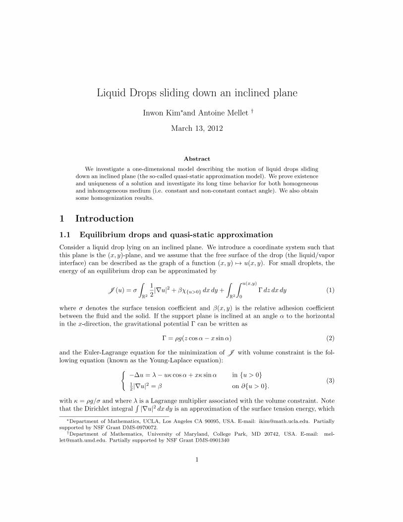
Note that the fact that r(q) can be zero in a non trivial interval is a classical and importantaspect of the homogenization of contact angle dynamics (see Figure 1). It typically impliespinning of the contact line: for related results in higher dimensions, we refer to [9] and [10].
We can now state our homogenization result:
Theorem 2.7. Let uε be a solution of (12) with initial value u0 and where β = β(x/ε) with β aperiodic function. When ε goes to zero, uε converges uniformly to a function u(x, t) solution of(14)-(15) satisfying the following velocity law:{
min{a′(t) + r( 12 |ux(a(t))|2), |ux(a(t))|} = 0
min{−b′(t) + r( 12 |ux(b(t))|2), |ux(b(t))|} = 0
a.e. t ≥ 0. (21)
Furthermore, there is at most one solution u of the homogenized problem (14)-(15)-(21) withgiven initial data u0.
To conclude this analysis, we note that the homogenized problem described in Theorem 2.7has traveling wave solutions for all volume (for small volume, the traveling wave has speed zero,so it is really a stationary solution). The speed of that traveling wave can be determined asfollows:
8

0 0.5 1 1.5 2 2.5−1
−0.8
−0.6
−0.4
−0.2
0
0.2
0.4
0.6
0.8
1
Figure 1: Homogenized velocity function r(q) as a function of the slope q when β is given byβ(x) = 1 + 0.3 sinx. The straight line is the curve y = q − 〈β〉
• If r(V0κ sinα) + r(0) < 0, then there exists q0 such that
r(q0 + V0κ sinα) + r(q0) = 0
and the speed of the traveling wave solution is given by
c = r(q0 + V0κ sinα) = −r(q0)
(note that q0 may not be unique, but c is unique).
• If r(V0κ sinα) + r(0) ≥ 0, then the speed of the traveling wave solution is given by
c = r(V0κ sinα)
(when this happens, the gradient in the rear of the drop of the traveling wave solution iszero)
Of course, we recover the speed of the traveling wave for constant coefficient β (formula (18))when we take r(q) = q − β. Figure 2 compares the speed of the traveling wave as a function ofV0κ sinα for the homogenized problem (21) when βε(x) = 1 + 0.3 sin(x/ε) (i.e. with the functionr shown in Figure 1) and for the constant case β = 〈βε〉 = 1. Note the Lipschitz corner nearV0κ sinα = 2 which corresponds to the critical volume for which the gradient in the rear of thedrop becomes zero.
The rest of the paper is devoted to the proof of these results.
3 Preliminaries
3.1 Another formulation for (12)
Definition 2.1 gives the most natural notion of solution for (12). However, it is not the mostpractical one. In this section, we derive an equivalent formulation which will be more convenient.
9

0 0.5 1 1.5 2 2.5 3 3.5 40
0.5
1
1.5
2
2.5
3
Figure 2: Speed of the traveling wave solution as a function of V0κ sinα for the homogenizedproblem (21) when βε(x) = 1 + 0.3 sin(x/ε) (solid line), and for the constant case β = 〈βε〉 = 1.
First, we note that if u is a solution in the sense of Definition 2.1, then u(·, t) solves:−uxx = λ(t)− uκ cosα+ (x− b(t))κ sinα in (a(t), b(t))
u(a(t), t) = u(b(t), t) = 0,∫u dx = V0.
(22)
It is tempting to replace (14)-(15) by (22); However, solutions of (22) might take negativevalues (for large intervals (a(t), b(t))). We thus write:
Definition 3.1. Given an initial data u0 satisfying (13), we say that u(x, t) is a solution of (12)if there exist some Lipschitz functions a(t) and b(t) satisfying
a(0) = a0, b(0) = b0
such that u(·, t) solves (22) for all t ≥ 0 and a(t), b(t) satisfy{min{a′(t) + 1
2 |ux(a(t))|2 − β(a(t)), ux(a(t))} = 0
b′(t) = 12 |ux(b(t))|2 − β(b(t)).
(23)
In this second formulation, the positivity of u in (a(t), b(t)) is enforced by the conditionux(a) ≥ 0. Indeed, we can show:
Lemma 3.2. Let u(·, t) be the solution of (22), then −ux(b(t), t) > 0. Furthermore, u(x, t) > 0in (a(t), b(t)) if and only ux(a(t), t) ≥ 0. In particular, Definitions 2.1 and 3.1 are equivalent.
Note that it might have seemed more natural to write the second equation in (23) as
min{−b′(t) +1
2|ux(b(t))|2 − β(b(t)),−ux(b(t))}.
However, lemma 3.2 shows that the condition −ux(b(t)) > 0 always holds.
10

Proof of Lemma 3.2. We drop the t dependence in what follows. Since V0 > 0, there existsx0 ∈ (a, b) such that u(x0) = maxx∈(a,b) u > 0. Since −u′′(x0) ≥ 0, (22) implies
λ+ (x0 − b)κ sinα ≥ u(x0)κ cosα > 0. (24)
Assume now that u has a local minimum at a point x1 ∈ (a, b). Then −u′′(x1) ≤ 0, and so (22)implies
λ+ (x1 − b)κ sinα ≤ u(x1)κ cosα.
Since u(x1) ≤ v(x0), we deducex1 ≤ x0,
and so we always have u(x) > 0 in (x0, b). In particular, we have −u′(b) ≥ 0. In order to showthat −u′(b) > 0, we note that (24) also implies λ > 0, and so the function h(x) = −µ(x − b)satisfies
−h′′ ≤ λ− hκ cosα+ (x− b)κ sinα = λ− [µκ cosα+ κ sinα](b− x)
in a neighborhood of b. A Hopf’s Lemma - type argument yields −u′(b) > 0.
Assume now that u′(a) ≥ 0, and that there exists x0 ∈ (a, b) such that u(x0) ≤ 0. Using theboundary conditions, we deduce that there exist at least three distinct points in [a, b] where u′
vanishes, and so there exists at least two distinct points y1, y2 in (a, b) where u′′ vanishes.Therefore, the function w = uκ cosα− λ− (x− b)κ sinα, which solves
w′′ = κ cosαw in (a, b)
is such that w′′(yi) = w(yi) = 0, i = 1, 2 and the maximum principle implies w = 0 in (y1, y2)and thus w = 0 in (a, b), which is impossible (look at the values of w at a and b).
We have thus shown that u′(a) ≥ 0 implies that u > 0 in (a, b). Conversely, if u > 0 in (a, b),it is readily seen that u′(a) ≥ 0.
Finally, we give a third definition which will be very useful later on. We will show in Propo-sition 3.5 (iv) that there exists a critical length `c > 0 (depending on the volume V0 and theinclination α) such that the solution of (22) is positive in (a(t), b(t)) if and only if b(t)−a(t) ≤ `c.This length `c is the longest possible length of the support of the drop. This leads to the followingthird formulation:
Definition 3.3. Given an initial data u0 satisfying (13), we say that u(x, t) is a solution of (12)if there exist some Lipschitz functions a(t) and b(t) such that u(·, t) solves (22) and
a(0) = a0, b(0) = b0
with {min{a′(t) + 1
2 |ux(a(t))|2 − β(a(t)), a(t)− b(t) + `c} = 0
b′(t) = 12 |ux(b(t))|2 − β(b(t)),
(25)
a.e. t ≥ 0.
Equivalently, denoting `(t) = b(t)− a(t), we can write:{max
{`′(t)−
[12 |ux(b(t))|2 + 1
2 |ux(a(t))|2 − β(a(t))− β(b(t))], `(t)− `c
}= 0
b′(t) = 12 |ux(b(t))|2 − β(b(t)),
(26)
where ux(b(t)) and ux(a(t)) only depends on l(t) (see Proposition 3.5 (iii)).We then have:
11

Proposition 3.4. Definition 3.1 and 3.3 are equivalent.
In order to prove this proposition, we will need to derive several important properties of thesolution of the obstacle problem (15), which is done in the next section. Proposition 3.4 will bean immediate consequence of Proposition 3.8 below.
3.2 Analysis of the obstacle problem (15)
Throughout this section, we fix a volume V0, and all constants will depends on V0, α and κ.Given a < b, we consider u solution of
u = argmin{F (v) ; v ∈ H10 (a, b), v ≥ 0,
∫ b
a
v(x) dx = V0}. (27)
Then classical arguments for obstacle type problems yield that u ∈ C1,1(a, b) solves
min{−u′′−λ− (x− b)κ sinα+uκ cosα, u} = 0 in (a, b), u(a) = u(b) = 0,
∫u dx = V0 (28)
(where λ ∈ R is determined by the volume constraint).The main properties of u are gathered in the following proposition:
Proposition 3.5. Let u be a C1,1 solution of (28), then:
(i) {u > 0} is an interval of the form (a′, b) and −u′(b) > 0.
(ii) u is the unique solution of (28), and is also solution of (27).
(iii) λ, −|{u > 0}|, −u′(b) and u′(a′) only depends on a and b through (b− a) and are decreasingfunctions of b− a.
(iv) There exists `c > 0 such that {u > 0} = (a, b) if and only if b−a ≤ `c. Furthermore, u′(a) > 0if and only if b− a < `c.
The critical length `c is the longest possible length of the support of the drop. We recall thatit depends on V0, κ and α. It will play a very important role in the analysis of our problem.
In view of (iii), we can define
G(b− a) :=1
2|u′(a)|2, H(b− a) :=
1
2|u′(b)|2 (29)
where u is the solution of (28). The functions ` 7→ G(`) and ` 7→ H(`) are then both monotonedecreasing, and multiplying the equation (28) by u′ and integrating over (a′, b) yields
1
2u′(b)2 − 1
2u′(a′)2 = κ sinαV0
orH(`)−G(`) = κ sinαV0. (30)
We also defineF : ` 7→ G(`) +H(`), (31)
which is a decreasing function as well.Finally, we have the following lemmas, which will be useful later on:
12

Lemma 3.6 (Lipschitz regularity). For all δ0 > 0, there exists C > 0 such that
0 ≤ H(`0)−H(`0 + η) ≤ Cη
and0 ≤ G(`0)−G(`0 + η) ≤ Cη
for `0 ≥ δ0 and η ≥ 0. In particular, it follows that H and G (and therefore F ) are locallyLipschitz on (0,∞).
Lemma 3.7 (Non-degeneracy). For all δ0 > 0 there exists c > 0 such that
H(`0)−H(`0 + η) ≥ cη (32)
for all `0 ≤ `c − δ0 and η such that `0 + η ≤ `c
Next, we consider the following boundary value problem with volume constraint:{−v′′ = λ− vκ cosα+ (x− b)κ sinα in (a, b)
v(a) = v(b) = 0 and∫v dx = V0.
(33)
where λ is a Lagrange multiplier for the volume constraint. Then, we have:
Proposition 3.8. Let v be the solution of (33). Then there exists `c depending on V0, α and κsuch that the followings are equivalent
(i) v′(a) ≥ 0
(ii) v ≥ 0 is also the solution of (27)
(ii) b− a ≤ `cFurthermore, v′(a) > 0 if and only if b− a < `c.
This proposition implies Proposition 3.4.The remainder of this section is devoted to the proof of these results.
Proof of Proposition 3.5.
(i) Let (c, d) be a connected component of {u > 0}, then
−u′′ = λ+ (x− b)κ sinα− uκ cosα (34)
in (c, d). Multiplying (34) by u′ and integrating over (c, d) yields:
u′(d)2 = u′(c)2 + 2κ sinα
∫ d
c
u dx > 0.
If d 6= b, then the regularity of u implies u′(d)2 = 0, a contradiction. So d = b, |u′(b)| > 0 and(c, b) is the only connected component of {u > 0}. We also have the following formula:
u′(b)2 − u′(a′)2 = 2κ sinαV0 (35)
13

(ii) To prove the uniqueness of the solution of (28), we assume that u1, u2 are two solutions of(28) (with λ1 and λ2 respectively). We know that {ui > 0} = (a′i, b) and we can assume (withoutloss of generality) that a ≤ a′2 ≤ a′1.
If v = u1 − u2, then−v′′ = λ1 − λ2 − vκ cosα in (a′1, b).
Furthermore, v(a′1) ≤ 0, v(b) = 0 and∫ ba′1v dx > 0. So v reaches its positive maximum value
somewhere in (a′1, b). We deduceλ1 ≥ λ2.
Next, we note that since
−u′′1 ≥ λ1 + (x− b)κ sinα− u1κ cosα in {a′2, b},
we also have−v′′ ≥ λ1 − λ2 − vκ cosα ≥ −vκ cosα in (a′2, b),
with v(a′2) = v(b) = 0 and∫ ba′2v dx = 0. If v 6= 0, then v has a (strictly) negative minimum value
in (a′2, b), a contradiction. We deduce v = 0 and so u1 = u2.
(iii) Equation (28) is invariant by translation, and thus the uniqueness obtained in (ii) impliesthat u(·+ b) and λ only depends on ` = (b− a) (in particular, u′(a) and −u′(b) only depends on`).
The proof of (ii) above also implies that λ is a decreasing function of (b − a). We now takea2 < a1 < b and let u1 (resp. u2) be the solution of (28) on the interval (a1, b) (resp. (a2, b)).The function v = u1 − u2 satisfies
v(a1) ≤ 0, v(b) = 0, and
∫ b
a1
v ≥ 0
so there exists a point x0 ∈ [a1, b) such that v(x0) = 0. Since
−v′′ + vκ cosα = λ1 − λ2 ≥ 0 in (x0, b),
the maximum principle gives v ≥ 0 in (x0, b). In particular, −v′(b) ≥ 0 and so
−u′1(b) ≥ −u′2(b).
Finally, if u′2(a2) = 0, then u′2(a2) ≤ u′1(a1), while if u′2(a2) > 0, then (35) implies
u′2(a2)2 = u′2(b)2 − 2κ sinαV0
andu′1(a′1)2 = u′1(b)2 − 2κ sinαV0 ≥ u′2(b)2 − 2κ sinαV0 = u′2(a2)2
hence a′1 = a1 and u′1(a1) ≥ u′2(a2).
(iv) Note that if {u > 0} 6= (a, b), then u is the unique solution of (28) in any interval larger than(a, b). So we can define
`c := min{` ; the solution of (28) in (0, `) satisfies {u > 0} 6= (0, `)}
14

We only need to show that this set is non empty (that is `c <∞), and that this is equivalent tou′(a) 6= 0.
Assume that {u > 0} 6= (a, b). Then
−u′′ ≤ λ+ (x− b)κ sinα in (a, b)
and so
−u′(b) + u′(a) ≤ λ(b− a)− 1
2(b− a)2κ sinα
Since u′(a) ≥ 0 and u′(b) ≤ 0, we deduce
(b− a)κ sinα ≤ λ
Since λ is a decreasing function of (b− a), this implies that (b− a) ≤ C for some constant C.
Finally, we note that if b− a < `c, then u′(a) > 0, while the regularity of u implies u′(a) = 0when b− a ≥ `c.
We now turn to the proof of the Lipschitz regularity of the functions G and H:
Proof of Lemma 3.6. Note that H and G are constant for ` ≥ `c, so we can always assume that
δ0 ≤ `0 ≤ `0 + η ≤ `c. (36)
We now consider the solution u of (28) with a = 0 and b = `0 and we denote by λ(`0) theLagrange multiplier appearing in (28). We recall that λ is a decreasing function of `0 and weclaim that
λ(`0)− λ(`0 + η) ≤ Cη (37)
for some constant C depending on δ0. To prove this, we consider v solution of the same equationas u (with the same λ) but on the interval (0, `0 + η) instead of (0, `0):
−v′′ = λ(`0) + (x− `0)κ sinα− vκ cosα in (0, `0 + η), v(0) = v(`0 + η) = 0.
We note that v ≥ u and that the function h = v − u solves
hκ cosα− h′′ = 0 on (0, `0).
In particular, on the interval (0, `0), h must take its positive maximum at x = `0. Now on(`0, `0 + η) we have h = v ≤ C1η for some C1 > 0 with C1 depending on δ0. We conclude thath ≤ C1η in (0, `0 + η) and thus ∫
v dx ≤ V0 + C ′1η (38)
for some constant C ′1 depending on δ0 and `c (recall that `0 + η ≤ `c).
Next, we consider w the solution of (28) with a = 0 and b = `0 + η (and so λ = λ(`0 + η)).The function g = v − w solves
gκ cosα− g′′ = σ
in (0, `0 + η), with g(0) = g(`0 + η) = 0, where (since λ is decreasing)
σ = λ(`0)− λ(`0 + η) + ηκ sinα > 0.
15

Finally, we note that the solution of −φ′′ = µσ in (0, `0 + η) with zero boundary conditionsatisfies φκ cosα − φ′′ ≤ σ, if µ is small enough. The comparison principle thus implies thatg ≥ φ and so ∫
gdx =
∫v dx− V0 ≥
∫φdx ≥ Cµσ
for some small µ > 0. Equation (38) implies
C ′1η ≥ Cµσ
and soλ(`0)− λ(`0 + η) ≤ Cη
which proves (37).
We can now prove the Lipschitz bounds for the functions H and G by comparing u (solutionof (28) on (0, `0)) and w (solution of (28) on (0, `0 + η)): The function q(x) = u(x)−w(x) solves
qκ cosα− q′′ = λ(`0)− λ(`0 + η) + ηκ sinα, in (0, `0)
with q(0) = 0 and q(`0) = −w(`0) ≤ 0. So (37) implies
qκ cosα− q′′ ≤ Cη in (0, `0), with q(0) = 0 and q(`0) ≤ 0.
We deduce q′(0) ≤ Cη and sou′(0) ≤ w′(0) + Cη
which proves our statement for G. The proof for H is similar (fixing b = 0 and choosing a = −`0or a = −`0 − η).
The proof of Lemma 3.7 follows from similar argument:
Proof of Lemma 3.7. We recall that `0 ≤ `c− δ0 and we fix b = 0, a2 = −(`0 + η) and a1 = −`0.We note that it is enough to prove (32) for η ≤ (`c − `0)/2, so that we can assume that `0 + η ≤`c − δ0/2.
We now consider u1 (resp. u2) the solution of (28) on the interval (a1, 0) (resp. (a2, 0)). Thefunction h = u1 − u2 satisfies in particular
h(a1) ≤ 0, h(0) = 0
and we are going to show that max(a1,0) h ≥ cη for some c > 0.
First of all, the volume constraint implies that∫ b
a1
h dx =
∫ a1
a2
u2 dx > 0 (39)
Furthermore, since `0 + η < `c − δ0/2 the monotonicity of G implies
u′2(a2) >√
2G(`c − δ0/2) > 0
16

and so u2(a1) ≥ cη for some c > 0. Also, Lemma 3.6 gives
h′(a1) = u′1(a1)− u′2(a1)
= G(`0)− u′2(a1)
≤ G(`0 + η) + Cη − u′2(a1)
≤ Cη + u′2(a2)− u′2(a1)
≤ Cη
We deduce that there exists c > 0 such that
h(a1) = −u2(a1) ≤ −cη and h′(a1) ≤ cη. (40)
Finally, we have −h′′ + hκ cosα = λ1 − λ2 in (a1, 0), and so (37) implies
0 ≤ −h′′ + hκ cosα ≤ Cη. (41)
Consider now g solution of −g′′ + gκ cosα = C on (a1, 0) with g(a1) = −c and g′(a1) = c.Then (40) and (41) imply that h ≤ ηg in (a1, 0).
Let now y0 ∈ (a1, 0) be such that g < 0 in (a1, y0) and g(y0) = 0 (y0 only depends on theconstant c and C appearing in (40) and (41)), then∫ y0
a1
h dx ≤ η∫ y0
a1
g dx ≤ −cη (42)
with c > 0.Equations (39) and (42) imply that ∫ 0
y0
h(x)dx ≥ cη
and so there exists a point z0 ∈ (y0, 0) where h(z0) ≥ cη. A Hopf’s lemma type argument (using(41)) now yields |h′(0)| > cη and so
|u′1(0)| > |u′2(0)|+ cη.
The result follows.
Proof of Proposition 3.8.
(i)⇒(ii) If v′(a) ≥ 0, then Lemma 3.2 implies that v > 0 in (a, b), and so v is also the solution of(28), and thus of (27).
(ii)⇒(iii) If v is solution of (33), then v ≥ 0 in (a, b), and since v cannot be zero a an interval of(a, b), we must have {v > 0} = (a, b). Proposition 3.5 (iv) gives b− a ≤ `c.
(iii)⇒(i) Finally, if b− a ≤ `c, then the solution u of (27) satisfies {u > 0} = (a, b), and is thusalso a solution of (33). If follows that v′(a) = u′(a) ≥ 0.
17

4 Proof of Theorem 2.2
4.1 Uniqueness and Comparison principle
In this section, we prove the comparison principle, Proposition 2.3, which also implies the unique-ness part of Theorem 2.2:
Proof of Proposition 2.3. Thanks to Proposition 3.4, we can assume that u is a solution in thesense of Definition 3.3. Using the notations of (29), we can rewrite (25) as follows{
min{a′(t) +G(`(t))− β(a(t)), `c − `(t)} = 0
b′(t) = H(`(t))− β(b(t)),(43)
with ` 7→ H(`) and ` 7→ G(`) monotone decreasing. We now define
f(t) = max{a1(t)− a2(t), b1(t)− b2(t)}.
Since the functions ai(t) and bi(t) are in W 1,∞loc (0,∞), f(t) is in W 1,∞
loc (0,∞) and we have
f ′(t) =
a′1(t)− a′2(t) if a1(t)− a2(t) > b1(t)− b2(t)
b′1(t)− b′2(t) if a1(t)− a2(t) < b1(t)− b2(t)
b′1(t)− b′2(t) = a′1(t)− a′2(t) if a1(t)− a2(t) = b1(t)− b2(t)
a.e. t ≥ 0
and so
f ′(t) =
{a′1(t)− a′2(t) if `2(t) > `1(t)
b′1(t)− b′2(t) if `2(t) ≤ `1(t)
When `2(t) > `1(t), we have in particular `1(t) < `c, and so (43) gives
a′1(t) = −G(`1(t)) + β(a1(t)), a′2(t) ≥ −G(`2(t)) + β(a2(t)).
We deduce
f ′(t) ≤
{G(`2(t))−G(`1(t)) + β(a1(t))− β(a2(t)) if `2(t) > `1(t)
H(`1(t))−H(`2(t))− β(b1(t)) + β(b2(t)) if `2(t) ≤ `1(t)
and the monotonicity of G and H implies
f ′(t) ≤
{K|a1(t)− a2(t)| if a1(t)− a2(t) > b1(t)− b2(t)
K|b1(t)− b2(t)| if a1(t)− a2(t) ≤ b1(t)− b2(t)
with K = ||β′||L∞ . We thus have
f ′(t) ≤ K|f(t)| a.e. t ≥ 0.
In particular, f ′+(t) ≤ Kf+(t) and so f+(t) ≤ f+(0)eKt, so if f(0) ≤ 0, then f(t) ≤ 0 a.e. t ≥ 0.
We also have f ′−(t) ≥ −Kf ′−(t) and so f−(t) ≥ f−(0)e−Kt, so if f(0) < 0, then f(t) < 0 a.e.t ≥ 0. The result follows.
18

4.2 Existence of a solution
Observe that, when β does not depend on x, formulation (26) implies that the problem can bereduced to solving first an equation for `(t), of the form
max{`′(t)− [F (`(t))− 2β], `(t)− `c} = 0} (44)
with F defined by (31), and then an equation for b(t) of the form
b′(t) = H(`(t))− β. (45)
When β depends on x however, one cannot decouple the equations for a and b. We will thus usea discrete scheme to prove the existence of solutions in this general framework.
4.2.1 Discrete-time scheme
To prove the existence of a solution for general coefficient β, we introduce a simple discrete timescheme (simpler than the gradient flow scheme described in the introduction): For h > 0 small,we describe the evolution of the drop as follows:
Assume that the support of the drop at time tn = nh is the interval (an, bn) and denote byun(x) the corresponding solution of (27). We define
an+1/2 = an +[β(an)− 1
2 |u′n(an)|2
]h
bn+1/2 = bn +[12 |u′n(bn)|2 − β(bn)
]h
Next, we define un+1 as the solution of the obstacle problem (27) with a = an+1/2 and b = bn+1/2.Proposition 3.5 (i) implies that there exists an+1 and bn+1 = bn+1/2 such that
{un+1 > 0} = (an+1, bn+1).
This scheme defines a sequence of functions {un(x)}n∈N and a sequence of intervals {(an, bn)}n∈N.We then define uh(x, t), ah(t) and bh(t) continuous piecewise linear functions such that
uh(x, nh) := un(x)
ah(nh) := an, bh(nh) := bn.
Our goal is now to pass to the limit h→ 0.
First, we observe that since bn+1 = bn+1/2, we have
bn+1 − bnh
=1
2|u′n(bn)|2 − β(bn). (46)
On the other hand, we only have an+1 ≥ an+1/2 and if an+1 > an+1/2, then u′n+1(an+1) = 0. Sowe can write
an+1 − anh
≥ β(an)− 1
2|u′n(an)|2, with equality if u′n+1(an+1) > 0,
which implies
min
{an+1 − an
h+
1
2|u′n(an)|2 − β(an), u′n+1(an+1)
}= 0. (47)
Finally, using Proposition 3.8, we can also write:
min
{an+1 − an
h+
1
2|u′n(an)|2 − β(an), an − bn + `c
}= 0. (48)
19

4.2.2 Limit h→ 0
We now study the limit h → 0 of the discrete model introduced above. Note that un satisfies,for some λn,
−u′′n = λn − unκ cosα+ (x− bn)κ sinα in (an, bn),
un(an) = un(bn) = 0,∫un dx = V0.
(49)
We then have the following proposition:
Proposition 4.1. For all n, the following holds:
(i) |u′n(an)| and |u′n(bn)| are uniformly bounded. More precisely, there exists a constant Mdepending only on κ, α, V0 and the initial data such that
|u′n(an)| ≤ |u′n(bn)| ≤M.
(ii) There exist constants ` > 0 and Λ depending only on κ, α, V0 such that bn − an ≥ ` and|λn| ≤ Λ.
(iii) ah(t) and bh(t) are uniformly Lipschitz continuous with respect to h and t.
Before proving this proposition, we show that it implies the existence of a solution (Theo-rem 2.2):
Proof of Theorem 2.2. Proposition 4.1 implies that ah(t), bh(t) and `h(t) = bh(t) − ah(t) areLipschitz continuous uniformly with respect to h and that there exists ` independent of h suchthat
` ≤ `h(t) ≤ `c ∀t ≥ 0. (50)
In particular there exists a subsequence h→ 0 and some Lipschitz continuous functions a(t) andb(t) such that
ah(t)→ a(t), bh(t)→ b(t) uniformly with respect to t ∈ [a, b]
for all a < b ∈ R.Next, we note that for any t ≥ 0, uh(x, t) solves
−uxx(·, t) = λ(`h(t))− κ cosαu+ (x− bh(t))κ sinα, in (ah, bh)
and so the function vh(x, t) = uh(ah(t) + x`h(t), t) solves
−vxx(·, t) = `h(t)2 [λ(`h(t))− κ cosαv + `h(t)(x− 1)κ sinα
], in (0, 1)
withvh(0, t) = vh(1, t) = 0.
In particular, it is readily seen that x 7→ vh(x, t) is bounded in C2(0, 1) uniformly with respectto t, and that vh and vhx are Lipschitz continuous with respect to t, uniformly with respect to h.Finally, vh converges locally uniformly (with respect to x and t) to a function v solution of
−vxx(·, t) = `(t)2
[λ(`(t))− κ cosαv + `(t)(x− 1)κ sinα] , in (0, 1) with v(0, t) = v(1, t) = 0.
20

Writing
uh(x, t) = vh(x− ah(t)
`h(t), t
),
we deduce that uh converges locally uniformly (with respect to x and t) to a function u solutionof
−uxx(·, t) = λ(`(t))− κ cosαu+ (x− b(t))κ sinα, in (a(t), b(t))
satisfying
u(a(t), t) = u(b(t), t) = 0 and
∫u(·, t)dx = V0.
Furthermore, uhx(ah(t), t) and uhx(bh(t), t) are Lipschitz continuous function in t, uniformlywith respect to h. We can thus pass to the limit in (46) and (48). For instance, we note that(46) implies
bh′(t) =
bn+1 − bnh
=1
2|u′n(bn)|2 − β(bn).
for t ∈ (nh, (n+ 1)h), and so the Lipschitz continuity in time implies
bh′(t) =
1
2|uhx(bh(t), t)|2 − β(bh(t)) +O(h) a.e. t ≥ 0
Passing to the limit t→ 0 and repeating this argument with (48) yields (25).
Proof of Proposition 4.1. For the sake of clarity, we drop the index n when no ambiguity ispossible.
(i) In view of Poposition 3.5, we only need to show that the length of the support b − a cannotbe too small: First, if u′(a) = 0, then Proposition 3.5 (iv) implies that b− a = `c, and (30) gives
1
2|u′(b)|2 = V0κ sinα.
Next, if u′(a) 6= 0, then (46) and (47) implies that the length of the interval b− a at the nexttime step will be given by
b− a+
[u′(b)2
2+u′(a)2
2− β(an)− β(bn)
]≥ b− a+
[u′(b)2
2− β(an)− β(bn)
]In particular, if |u′(b)| ≥ 2 sup
√β, then the length of the interval increases and therefore |u′(b)|
decreases. We deduce that if u′(a) 6= 0, then
|u′(a)| ≤ |u′(b)| ≤ max{2 sup√β, |u′0(b)|}
and the result follows.
(ii) The proof of (i) above clearly implies that b− a is bounded below. Furthermore, integratingthe equation satisfied by u over (a, b), we get:
λ(b− a) = u′(a)− u′(b) + V0κ sinα− 1
2(b2 − a2)κ sinα
≤ 2M + V0κ sinα.
The result follows.
21

(iii) The discrete motion law (46) and (i) imply that there exists a constant C > 0 such that∣∣∣∣bn+1 − bnh
∣∣∣∣ ≤ C for all n ≥ 0.
Similarly, if |u′n+1(an+1)| 6= 0 then (47) and (i) imply∣∣∣∣an+1 − anh
∣∣∣∣ ≤ C for all n ≥ 0.
Finally, if u′n+1(an+1) = 0, then bn+1 − an+1 = `c and since bn − an ≤ `c we have
an+1 − anh
≤ bn+1 − bnh
≤ C,
and (47) impliesan+1 − an
h≥ β(an)− 1
2M2 ≥ −1
2M2.
The result follows.
5 Asymptotic behavior when β is constant: Existence oftraveling wave solutions
In this section, we study the long time behavior of the drops when β is constant (homogeneousmedia), and prove Theorem 2.4.
As mentioned earlier, Problem (12) is much simpler in this case since the length of the support`(t) = b(t)− a(t) solves
max {`′(t)− [F (`(t))− 2β] , `(t)− `c} = 0 (51)
with F defined by (31). Once the solution of (51) is found, the solution of (12) is fully determinedby solving
b′(t) = H(`(t))− β.
A traveling waves type solution of (22)-(25) is a solution of the form
u(x, t) = v(x− ct).
For such a solution, the endpoints of the support (a(t), b(t)) of u satisfy
a′(t) = c and b′(t) = c for all t. (52)
and the length b(t)− a(t) is constant equal to some `0. Equation (51) thus reduces to finding `0such that
max {− [F (`0)− 2β] , `0 − `c} = 0. (53)
To solve this equation, we recall that F is continuous and monotone decreasing on the interval(0, `c]. So we have the following:
1. Either F (`c) < 2β, in which case, there exists a unique `0 < `c such that F (`0) = 2β.
2. Or F (`c) ≥ 2β, in which case we have `0 = `c.
22

This proves the existence of a unique traveling wave, and we now derive the formula (18) forthe speed c: Let a and b be such that b− a = `0 and let u be the corresponding solution of (7)with support (a, b). If ux(a) > 0 , then (25) and (52) imply
1
2|ux(a)|2 = β − c, 1
2|ux(b)|2 = β + c
and so (30) yields
c =1
2(H(`0)−G(`0)) =
1
2V0κ sinα.
This is possible only if β − c = 12 |ux(a)|2 > 0, that is if 1
2V0κ sinα < β.If ux(a) = 0, then (52), (25) and (30) imply
c = H(`0)− β = V0κ sinα− β.
This implies formula (18).
Finally, the stability of `0 is an immediate consequence of the monotonicity of F since itimplies that any solution of (51) satisfies{
`′(t) < 0 if ` < `0`′(t) > 0 if ` > `0.
and so `(t) → `0 as t → ∞. Since the profile u(x, t) is completely determined by the length ofthe support, the convergence of `(t) implies the uniform convergence of u(x, t) to the profile ofthe unique traveling wave.
6 Asymptotic behavior when β is periodic: Existence ofpulsating traveling solutions
In this section, we investigate the long time behavior of the solution when the function β isperiodic, and prove Theorem 2.5. This is of course more delicate than the case where β isconstant, since we cannot reduce (12) to a single equation for the length `(t) of the support.
First, we observe that for any solution we have (using (30)):
a′(t) + b′(t) ≥ 1
2|ux(b(t))|2 − 1
2|ux(a(t))|2 + β(a(t))− β(b(t))
≥ V0κ sinα+ β(a(t))− β(b(t)). (54)
In particular the condition
maxβ −minβ < V0κ sinα+ δ for some δ > 0 (55)
guarantees that a′(t) + b′(t) > δ for all time. This implies that no stationary solution can existunder condition (55), and that any drops must slide down the inclined plane.
In order to prove the first part of Theorem 2.5 (existence and stability of Pulsating travelingsolutions), we will prove that (55) actually implies that b′(t) > 0 for all (large enough) time,and that we can thus rewrite the equations for a(t) and b(t) using x = b(t) instead of t as aparameter. We thus start with the following lemma:
23

Lemma 6.1. The function t 7→ b(t) is in C1,1 and if (55) holds then there exists η > 0 such thatb′(t) > η at least for t ≥ T0 = 2 δ
`(0) .
Proof. Let η ∈ (0, δ/8) be a small number, to be chosen later. Equation (54) and condition (55)implies
a′(t) + b′(t) > δ, for all t ≥ 0. (56)
So as long as b′(t) ≤ η, we have a′(t) ≥ δ − η and thus
`′(t) = b′(t)− a′(t) ≤ −δ + 2η ≤ −δ/2.
In particular, we cannot have b′(t) ≤ η in (0, T0) (with T0 = 2 δ`(0) ), or the length of the droplet
would shrink to a point.Therefore if the lemma is false, then there exists t0 > t1 such that b′(t0) = η and b′(t) ≥ η
for t ∈ (t1, t0). Next, we note that t 7→ `(t) and t 7→ b(t) are Lipschitz continuous and so (43)implies that t 7→ b′(t) is also Lipschitz continuous. Therefore, there exists h ≤ η
K (where K isthe Lipschitz constant of b′) such that
b′(t) < 2η for t ∈ (t0 − h, t0). (57)
Proceeding as before (using the fact that η < δ/8), we deduce that
`′(t) < −δ/2 for t ∈ (t0 − h, t0)
and so
`(t0) < `(t0 − h)− δ
2h
(in particular, `(t) < `c and so ux(a(t), t) > 0 for t ∈ (t0 − h, t0)). Lemma 3.7 implies
H(`(t0)) ≥ H(`(t0 − h)) + c0δh (58)
for some c0 > 0. Finally, (57) implies
|b(t0)− b(t0 − h)| ≤ 2hη
and so (43) gives
η = b′(t0) = H(`o)− β(b(t0)) > H(`(t0 − h)) + c0δh− β(b(t0 − h)− ||β′||∞2hη
> b′(t0 − h) + c0δh− ||β′||∞2hη
Since we can always choose h such that b′(t0 − h) > η (by taking h ≤ t0 − t1), we obtain acontradiction if we choose η such that
η <c0δ
2||β′||∞.
Proof of Theorem 2.5 (i). Lemma 6.1 implies that t 7→ b(t) is bijective from (T0,∞) onto (b(T0),∞).We can thus re-parametrize the motion of the drop using x = b(t) as our new parameter. Wenow write the equation satisfied by y(x) = `(b−1(x):
max{y′(x)b′(b−1(x))− [F (y(x))− β(a(b−1(x)))− β(x)], y(x)− `c} = 0.
24

Using the fact that b′(b−1(x)) > 0 and a(t) = b(t)− `(t), the equation can be written as
max{y′(x)− 1
b′(b−1(x))[F (y(x))− β(x− y(x))− β(x)], y(x)− `c} = 0.
Finally, using the equation for b′(t), we deduce that y solves
max{y′(x)−F(y(x), x), y(x)− `c} = 0. (59)
with
F(x, y) =F (y(x))− β(x− y(x))− β(x)
H(y(x))− β(x).
In particular, the function (x, y) 7→ F(x, y) is periodic with respect to x.
We now need the following lemma which will be proved later on:
Lemma 6.2. There exists a 1-periodic function z(x) such that
limn→∞
y(n+ x) = z(x).
In order to conclude, we rewrite the equation for b(t) as
b′(t) = H(y(b(t)))− β(b(t))
= H(b(t)) + ϕ(b(t))
with H(b) := H(z(b))− β(b) periodic function, and ϕ(b) := H(y(b))−H(z(b)) satisfying
|ϕ(b)| −→ 0 as b→∞.
Since b′(t) ≥ η, there exists a sequence tn → ∞ such that b(tn) = n. Let us considerbn(t) := b(tn + t)− n, which solves the following equation:
b′n(t) = H(bn(t)) + ϕ(bn(t) + n), bn(0) = 0.
We deduce|bn+k(t)− bn(t)| ≤ eCt(|ϕ(n)|+ |ϕ(n+ k)|),
and thus {bn} is a Cauchy sequence: it converges to a monotone increasing function b∞(t). Since
bn(tn+1 − tn) = bn+1(0) + 1,
we deduce that tn+1 − tn converges to the unique t0 satisfying b∞(t0) = 1 and that b∞ ist0-periodic.
Hence, we can show that b(t) − b∞(t) converges to 0 as t goes to ∞, and defining `∞(t) =z(b∞(t)), and a∞(t) = b∞(t)− `∞(t), we obtain a pulsating solution (a∞(t), b∞(t)).
Lastly, the uniqueness of the pulsating solution with positive speed (which is guaranteed byLemma 6.1) follows from the comparison principle (Proposition 2.3).
25

Proof of Lemma 6.2. We recall that y(x) is a bounded solution of (59). For n ∈ N, we denoteyn(x) = y(x+n). The periodicity of F with respect to x implies that it is also a bounded solutionof (59) with initial condition yn := y(n).
If y1 = y0, then the uniqueness implies that y(x + 1) = y(x) for all x and we can takez(x) = y(x). Otherwise, if, for instance y1 > y0, then the uniqueness implies that y1(x) ≥ y0(x)for all x ≥ 0 and so y2 = y1(1) ≥ y0(1) − y1. We deduce y2(x) ≥ y1(x), and iterating thisargument, we get
yn+1(x) ≥ yn(x) for all n ∈ N.
So {yn(x)} is monotone and bounded, and thus there exists z(x) such that limn→∞ yn(x) = z(x).Since yn(x+ 1) = yn+1(x), it follows that z(x+ 1) = z(x), which completes the proof.
To complete the proof of Theorem 2.5, it remains to investigate the case where
maxβ −minβ ≥ V0κ sinα+ δ (60)
for some δ > 0. The comparison principle (Proposition 2.3) implies that stationary solutions actas barrier and prevents the motion of the drop down the inclined plane. However, condition (60)does not automatically imply the existence of a stationary solution. Nevertheless, we can showthat stationary solutions do not exist provided the period of β is small enough.
Proof of Theorem 2.5 (ii). We denote by L the period of β.We first fix `0 such that H(`0) = maxβ. We note that we can always find such an `0.
Indeed, H(`) → +∞ as ` → 0, and using the fact that G(`c) = 0 together with (30), we getH(`c) = V0κ sinα. Condition (60) thus implies
H(`c) = V0κ sinα < maxβ −minβ < maxβ.
and the intermediate value theorem implies the existence of `0 < `c such that H(`0) = maxβ.We now fix a such that β(a) = minβ, and we find b ∈ [a+`0, a+`0+L] such that β(b) = maxβ
(we can always find such a b thanks to the periodicity of β).Consider now the solution of (7) with support (a, b). Since `0 ≤ b− a ≤ `0 + L, we have
1
2|ux|2(b) = H(b− a) ≤ H(`0) = maxβ
and so (thanks to the choice of b)
1
2|ux|2(b)− β(b) ≤ 0. (61)
We also have (using Lemma 3.6, and the fact that `0 < `c)
1
2|ux|2(a) = G(b− a) ≥ G(`0 + L) ≥ G(`0)− CL, (62)
as long as L ≤ 12 (`c − `0). Finally, (30) implies
G(`0) = H(`0)− V0κ sinα = maxβ − V0κ sinα.
In particular (62) yields1
2|ux|2(a) ≥ β(a) = minβ
26

as soon asmaxβ −minβ ≥ V0κ sinα+ CL
which holds for all L ≤ δ0 in view of (60). Therefore we deduce
β(a)− 1
2|ux|2(a) ≤ 0 (63)
The comparison principle together with (61) and (63) implies that if a(0) ≤ a and b(0) ≤ b,then the corresponding solution will satisfy
a(t) ≤ a and b(t) ≤ b for all t ≥ 0,
hence the result.
7 Homogenization of the velocity law
We now prove our last result, Theorem 2.7. Recall that the function r(q) is defined for all q 6= 0as in (20), as the effective speed of the global (periodic) solution of the ODE
x′(t) = q − β(x(t)). (64)
(see Lemma 2.6, whose proof is provided in appendix A).
Now, let uε(x, t) solve the inhomogeneous problem with period ε and with given initial datau0. We also denote by aε(t) and bε(t) the left and right endpoints of the support of uε.
Convergence. First, we obtain a priori estimate on uε in the same way that we did in theconstruction of a solution in Section 4.2:
We recall that aε(t), bε(t) and `ε(t) = bε(t)− aε(t) are Lipschitz continuous (bounded speedof the endpoints) uniformly with respect to ε and there exists ` independent of ε such that
` ≤ `ε(t) ≤ `c ∀t ≥ 0. (65)
In particular there exists a subsequence ε→ 0 and some Lipschitz continuous functions a(t)and b(t) such that
aε(t)→ a(t), bε(t)→ b(t) uniformly with respect to t ∈ [a, b]
for all a < b ∈ R.Next, we note that for any t ≥ 0, uε(x, t) solves
−uxx(·, t) = λ(`ε(t))− κ cosαu+ (x− bε(t))κ sinα, in (aε, bε)
and so the function vε(x, t) = uε(aε(t) + x`ε(t), t) solves
−vxx(·, t) = `ε(t)2
[λ(`ε(t))− κ cosαv + `ε(t)(x− 1)κ sinα] , in (0, 1)
withvε(0, t) = vε(1, t) = 0.
27

In particular, it is readily seen that x 7→ vε(x, t) is bounded in C2(0, 1) uniformly with respectto t, and that vε and vεx are Lipschitz continuous with respect to t, uniformly with respect to ε.Finally, vε converges locally uniformly (with respect to x and t) to a function v solution of
−vxx(·, t) = `(t)2
[λ(`(t))− κ cosαv + `(t)(x− 1)κ sinα] , in (0, 1) with v(0, t) = v(1, t) = 0.
Writing
uε(x, t) = vε(x− aε(t)`ε(t)
, t
),
we deduce:
Lemma 7.1. The function x 7→ uε(x, t) is bounded in C2(aε, bε) uniformly w.r.t. t, and uε anduεx are Lipschitz continuous with respect to t, uniformly with respect to ε. Finally, uε convergeslocally uniformly (with respect to x and t) to a function v solution of
−uxx(·, t) = λ(`(t))− κ cosαu+ xκ sinα, in (a(t), b(t)) with u(a(t), t) = u(b(t), t) = 0
and ∫u(·, t)dx = V0.
We can now prove Theorem 2.7:
Proof of Theorem 2.7. We first consider the equation for bε(t), which reads
bε′(t) = H(`ε(t))− β(bε(t)/ε).
Since t 7→ `ε is a Lipschitz continuous function, we can also write
bε′(t) = qε(t)− β(bε(t)/ε)
with qε(t) uniformly (w.r.t. ε) Lipschitz function converging (uniformly) to q(t) = H(`(t)).For a given t0 > 0, the function
xε(t) =1
εbε(t0 + εt)
solvesxε′(t) = qε(t0 + εt)− β(xε(t)).
Since qε(t0 + εt) is Lipschitz and qε(t0) converges to q(t0), we have that for all δ > 0, there existsε0 such that
|qε(t0 + εt)− q(t0)| ≤ δ +Kεt ∀ε < ε0, ∀t.
and so
|qε(t0 + εt)− q(t0)| ≤ 2δ ∀ε < ε0, ∀|t| ≤ δ
Kε. (66)
It follows that
xε′(t) ≤ q(t0) + 2δ − β(xε(t)) ∀ε < ε0, ∀|t| ≤ δ
Kε.
and
xε′(t) ≥ q(t0)− 2δ − β(xε(t)) ∀ε < ε0, ∀|t| ≤ δ
Kε.
28

Denoting by x (respectively x) the solution of (64) with q = q(t0) + 2δ (respectively q =q(t0)− 2δ) satisfying x(0) = x(0) = xε(0), we deduce
x(t) ≤ xε(t) ≤ x(t) ∀ε < ε0, 0 ≤ t ≤ δ
Kε. (67)
x(t) ≤ xε(t) ≤ x(t) ∀ε < ε0, − δ
Kε≤ t ≤ 0. (68)
Equation (67) implies
r(q(t0)− 2δ)t− 1 ≤ xε(t)− xε(0) ≤ r(q(t0) + 2δ)t+ 1 ∀ε < ε0, 0 ≤ t ≤ δ
Kε
and so
r(q(t0)− 2δ)t− ε ≤ bε(t0 + t)− bε(t0) ≤ r(q(t0) + 2δ)t+ ε ∀ε < ε0, 0 ≤ t ≤ δ
K.
Passing to the limit ε→ 0, we deduce
r(q(t0)− 2δ) ≤ b(t0 + t)− b(t0)
t≤ r(q(t0) + 2δ) 0 ≤ t ≤ δ
K.
and taking the limit t → 0+ and then δ → 0, we obtain (using the continuity of the functionq 7→ r(q)):
r(q(t0)) ≤ lim inft→0+
b(t0 + t)− b(t0)
t≤ lim sup
t→0+
b(t0 + t)− b(t0)
t≤ r(q(t0)).
Furthermore, using (68) instead of (67), we can show that a similar inequality holds for the limitt→ 0+. We thus deduce that b is differentiable at t0 and satisfies
b′(t0) = r(q(t0))
where q(t0) = H(`(t0)) = 12 |ux(b(t0), t0)|2.
The equation for aε(t) is handled in a similar fashion. Recall that
−aε′(t) ≤ G(`ε(t))− β(aε(t)/ε),
with equality if |uεx(aε(t))| > 0.If limε→0 |uεx(aε(t0))| > 0, then we have |uεx(aε(t))| > 0 for t in a neighborhood of t0 and for
small ε, and the argument presented above applies. If limε→0 |uεx(aε(t0))| = 0, then the aboveargument applies, but we have q(t0) = 0 and so we only get
−aε(t0 + t) + aε(t0) ≤ r(2δ)t+ ε ∀ε < ε0, 0 ≤ t ≤ δ
K.
Passing to the limit ε→ 0, we deduce
−a(t0 + t)− a(t0)
t≤ r(2δ) 0 ≤ t ≤ δ
K.
29

and taking the limit t → 0+ and then δ → 0, we obtain (using the continuity of the functionq 7→ r(q)):
lim supt→0+
−a(t0 + t)− a(t0)
t≤ r(0).
and a similar limit for t→ 0+.This prove that uε converges (up to a subsequence) to a solution of (14), (15), (21).
To complete the proof of Theorem 2.7, it remains to prove the uniqueness of the solutionof the homogenized problem, which also implies the convergence of the whole sequence uε to u.For that, we will show that a comparison principle similar to that of Proposition 2.3 holds (notethat we cannot deduce this comparison principle by passing to the limit ε→ 0 in Proposition 2.3since two solutions of the homogenized problem may be obtained by passing to the limit alongdifferent subsequences of ε).
Using the notations of (29) we first rewrite (21) as follows{min{a′(t) + r(G(`(t))), `c − `(t)} = 0
b′(t) = r(H(`(t))).(69)
We now consider two solutions of the homogenized problem u1 and u2 with initial data withsupport (a1(0), b1(0)) and (a2(0), b2(0)) satisfying
a1(0) ≤ a2(0) , and b1(0) ≤ b2(0).
We then definef(t) = max{a1(t)− a2(t), b1(t)− b2(t)}.
Since the functions ai(t) and bi(t) are in W 1,∞loc (0,∞), f(t) is in W 1,∞
loc (0,∞) and we have
f ′(t) =
{a′1(t)− a′2(t) if `2(t) > `1(t)
b′1(t)− b′2(t) if `2(t) ≤ `1(t)
When `2(t) > `1(t), we have in particular `1(t) < `c, and so (69) gives
a′1(t) = −r(G(`1(t))), a′2(t) ≥ −r(G(`2(t))).
We deduce
f ′(t) ≤
{r(G(`2(t)))− r(G(`1(t))) if `2(t) > `1(t)
r(H(`1(t)))− r(H(`2(t))) if `2(t) ≤ `1(t)
and the monotonicity of G, H and r implies
f ′(t) ≤ 0.
We deduce that if f(0) ≤ 0, then f(t) ≤ 0 a.e. t ≥ 0 which implies the comparison result, andthe uniqueness of the solution.
30

A The function r(q): Proof of Lemma 2.6
In this section, we prove Lemma 2.6. We recall that β is a periodic function (with period 1 forinstance) and for a given q ≥ 0, we consider the following equation:
x′(t) = q − β(x(t)). (70)
Since β is a Lipschitz function, (70) has a unique solution for any initial data x(0) = x0 and twosolutions can never cross.
Our first remark is that if q ∈ [minβ,maxβ], then any solution of (70) will be trapped in thesense that x(t) ∈ [x(0) − 1, x(0) + 1] for all t. Indeed, periodicity of β implies that there existsx1 ∈ [x(0) − 1, x(0)) and x2 ∈ (x(0), x(0) + 1] such that q − β(x1) ≥ 0 and q − β(x2) ≤ 0. It isthen easy to show that x(t) ∈ [x1, x2] for all t.
In that case, the effective speed of any solutions of (70) is zero. We thus have
r(q) = 0 , q ∈ [minβ,maxβ].
For q > maxβ and q < minβ, on the other hand, any solution of (70) will be strictlymonotone, with limt→±∞ x(t) = ±∞. In particular, we can then show that all solutions areequal, up to a translation in time. Assuming that x(0) = 0 (without loss of generality), thereexist a unique tc such that x(tc) = 1. Uniqueness for (70) implies that t 7→ x(t) is then periodicwith period tc and that its effective speed is given by
r(q) =1
tc
We then have
Proposition A.1. The function r : q 7→ r(q) defined above is a non-decreasing function. Fur-thermore,
(i) q 7→ r(q) is locally Lipschitz in (maxβ,∞) and [0,minβ)
(ii) If q0 = maxβ, then we have
r(q) ≤ C(q − q0)1/2 for q ≥ q0
if x 7→ β is C2, andr(q) ≤ C(− ln(q − q0))−1 for q ≥ q0
if x 7→ β is only Lipschitz. In particular r is a continuous function in [0,∞)
Proof of Proposition A.1. To prove the first part, we consider q2 > q1 > maxβ and we setη = q2 − q1. Let x(t) and y(t) be the solution of (70) with q = q1 and q = q2 respectively, andx(0) = y(0) = 0. Since x′(t) ≥ q1 −maxβ = δ > 0, we can define
h(s) = y ◦ x−1(s)− s,
solution of
h′(s) =q1 − β(x+ h(x)) + η
q1 − β(x)− 1
=β(x)− β(x+ h(x)) + η
q1 − β(x)
≤ K
δ(h(x) + η)
31

Since h(0) = y(x−1(0))− 0 = 0, the Gronwall’s lemma implies
h(1) ≤ Cη. (71)
If we denote tc such that x(tc) = 1 (so that r(q1) = 1/tc), then (71) implies
y(tc) ≤ 1 + Cη.
Finally, since y′(t) ≥ δ, this implies t2, such that y(t2) = 1 satisfies t2 ≥ tc − Cη and so
r(q2) ≤ r(q1) + Cη
for some C depending on q1 and r(q1).
The constant C degenerates when r(q) goes to zero, so we need different argument to prove(ii): Let η = q− q0. Assume (with loss of generality) that maxβ = β(0) (and so β′(0) = 0). If βis C2, then
β(x) ≥ β(0)− Cx2 = q0 − Cx2, for all x
and soq − β(x) ≤ η + Cx2.
Let now x(t) be the corresponding solution of (70). Up to a translation in time, we can alwaysassume that x(0) = 0. We then have
x′(t) ≤ η + Cx(t)2
We deduce
x(t) ≤ Cηt
1− C√ηtfor t ≤ (C
√η)−1.
In particular, tc, defined by x(tc) = 1 satisfies
1
tc≤ C(η +
√η)
hence the first result.When β is only Lipschitz, a similar argument yields
x′(t) ≤ η + Cx(t)
which gives the second result.
References
[1] T.D. Blake and K. J. Ruschak, Wetting: Static and dynamic contact lines, In Liquid FilmCoating-Scientific Principles and their Applications. Chapmann & Hall 1997.
[2] L.A. Caffarelli, A. Mellet, Capillary drops: Contact angle hysteresis, Calc. Var. PartialDifferential Equations 29 (2007), no. 2, 141–160.
[3] R. Finn, Equilibrium Capillary Surfaces, Grundlehren der Mathematischen Wis-senschaften [Fundamental Principles of Mathematical Sciences], Springer-Verlag, 1986.
32

[4] K. Glasner, I. Kim, Viscosity solutions for a model of contact line motion. Interfaces FreeBound. 11 (2009), no. 1, 3–60.
[5] H. P. Greenspan, On the motion of a small viscous droplet that wets a surface. J. FluidMech. (1978) 84, pp. 125–143.
[6] N. Grunewald and I. Kim, A variational approach to a quasi-static droplet model. Calc.Var. PDE (2011) 41 pp.1–19.
[7] L. M. Hocking and M. J. Miksis, Stability of a ridge of fluid, J. Fluid Mech. (1993) 247pp.157–177.
[8] R. Jordan, D. Kinderlehrer and F. Otto,The variational formulation of the Fokker-Planckequation. SIAM J. Math. Anal. (1998) 29, pp.1–17.
[9] I. Kim, Homogenization of a model problem on contact angle dynamics, Comm. PartialDifferential Equations (2008) 33, no. 7-9, pp. 1235–1271.
[10] I. Kim, Error estimates on homogenization of free boundary velocities in periodic media,Ann. Inst. H. Poincar Anal. Non Lineaire (2009)26, no. 3, pp. 999–1019.
[11] I. Kim, A. Mellet, Homogenization of a Hele-Shaw problem in periodic and random media,Arch. Rat. Mech. Ana., 194 (2009), no. 2, 507–530.
[12] N. Le Grand, A. Daerr, L. Limat, Shape and motion of drops sliding down an inclinedplane, J. Fluid Mech. 541 (2005), pp. 293–315.
33