Embed Size (px)
Citation preview

Linux Kernel Support
For Micro-Heterogeneous Computing
by
Kim R. Schuttenberg
A Thesis Submitted in
Partial Fulfillment of the Requirements for the Degree of
Masters of Science in
Computer Engineering Dr. Muhammad Shaaban
Assistant Professor, Department of Computer Engineering
Dr. Greg Semeraro
Dr. James Heliotis
Department of Computer Engineering Kate Gleason College of Engineering
Rochester Institute of Technology Rochester, New York
June 2004

ii
Release Permission Form Rochester Institute of Technology
Linux Kernel Support For
Micro-Heterogeneous Computing
I, Kim Schuttenberg, hereby grant permission to the Wallace Library of the Rochester
Institute of Technology to reproduce my thesis in whole or in part, on or after July 1,
2004. Any reproduction will not be for commercial use or profit.
Kim Schuttenberg Date

iii
ABSTRACT
Heterogeneous Computing (HC) is a technique speeds the computation of large
tasks by utilizing multiple computers or supercomputers, each of which is best suited to a
particular type of computation. Micro-Heterogeneous Computing (MHC) has been
proposed to bring this practice to individual computers. With the aid of the higher speed,
short distance interconnects found within the next generation of personal computers and
commodity servers, it should be possible to apply HC to relatively small grain sizes.
MHC draws on the observations that in order for a new computing technology to
become widely accepted, and cost effective, there must be a suitable abstraction layer that
frees the application writers from the need of precise technical knowledge about the
system. MHC provides such an abstraction layer, referred to as the MHC framework,
which provides automated solutions to many of the problems that must be overcome
when utilizing HC. The framework was designed with the goals of user transparency,
flexibility, and performance.
The problems addressed include matching tasks to devices and scheduling them
(collectively known as mapping), dependency analysis, and parallelization of serial code.
All of these problems are solved dynamically at run time by the framework whose
implementation is discussed herein. In support of this framework, this thesis specifies a
format for libraries that provide common functions and free their users from the tasks of
code profiling and analytical benchmarking.
This thesis provides the first implementation for such an abstraction layer by
utilizing the Linux operating system. This thesis provides not only the kernel level
support necessary to schedule tasks to hardware, but also implements the entire core
framework, with functioning solutions to the problems mentioned above. This thesis
provides well-defined interfaces and methods to expand the MHC system with new
scheduling heuristics, function libraries, and device drivers.
iv
Table of Contents Abstract .........................................................................................................................iii
Glossary.........................................................................................................................vi
1 Introduction.............................................................................................................. 1
1.1 General Overview .................................................................................................... 1
1.2 Previous Work ......................................................................................................... 3
1.3 Work in This Thesis ................................................................................................. 4
2 Micro-Heterogeneous Computing Overview ............................................................ 8
2.1 Background.............................................................................................................. 8
2.2 Micro-Heterogeneous Computing General Concepts .............................................. 13
2.3 Implementation Overview...................................................................................... 15
3 MHC Hardware...................................................................................................... 17
3.1 Classification ......................................................................................................... 17
4 Component Interfacing........................................................................................... 22
4.1 Overview ............................................................................................................... 22
4.2 Data Parameterization Method ............................................................................... 22
4.3 Task Representation ............................................................................................... 24
4.4 Device Configuration Representation ..................................................................... 25
4.5 Driver Interface...................................................................................................... 27
4.6 Kernel Interface ..................................................................................................... 34
4.7 Base Library Internal Interface ............................................................................... 37
4.8 Base Library User Application Interface................................................................. 41
4.9 User/Function Library Interface ............................................................................. 46
4.10 Notes on Included Example Library ....................................................................... 54
5 Automatic Parallelization ....................................................................................... 55
5.1 Overview ............................................................................................................... 55
5.2 Building the Task Graph ........................................................................................ 57
5.3 Functionality Exposed to the User .......................................................................... 64

v
5.4 Error Handling in an Automatically parallelized system ......................................... 64
5.5 Interaction with OS Provided primitives................................................................. 65
5.6 Breaking up task automatically............................................................................... 66
6 Scheduling Heuristic Implementation..................................................................... 68
6.1 Overview ............................................................................................................... 68
6.2 Statistics Collection................................................................................................ 68
6.3 Online Scheduler.................................................................................................... 69
6.4 Batch Scheduler ..................................................................................................... 73
7 Reconfiguration Latency Handling......................................................................... 77
7.1 Previous Work ....................................................................................................... 77
7.2 Hardware solutions................................................................................................. 78
7.3 Configuration Sharing............................................................................................ 78
7.4 Online Scheduler Reconfiguration Latency Hiding................................................. 78
7.5 Batch Scheduler Reconfiguration Latency Hiding .................................................. 80
8 Performance Analysis and Testing ......................................................................... 83
8.1 Performance Analysis ............................................................................................ 83
8.2 Testing environment............................................................................................... 91
8.3 Experiments Performed.......................................................................................... 93
9 Results ................................................................................................................. 101
9.1 Submission Time.................................................................................................. 101
9.2 Basic Scheduling Results ..................................................................................... 107
9.3 Reconfiguration Latency Handling....................................................................... 115
10 Future Work......................................................................................................... 120
10.1 Overview ............................................................................................................. 120
10.2 Caching and Coherency........................................................................................ 120
10.3 Automatic Task Aggregation................................................................................ 121
10.4 ETC Prediction/Automatic Profiling..................................................................... 122
10.5 Memory Locking Option for Jobs with small memory regions.............................. 122
10.6 Impact of Dynamic Queues on MHC.................................................................... 124
10.7 Back Annotation of ETC predictions to improve accuracy.................................... 124
10.8 Integration of more options for ETC prediction .................................................... 125

vi
10.9 Creation of MHC compliant hardware / drivers / libraries..................................... 125
10.10More/Better Batch Scheduling Heuristics ........................................................... 125
10.11“Stackable” batch schedulers. ............................................................................. 126
11 Conclusion ........................................................................................................... 127
12 References ........................................................................................................... 129

vii
Glossary
Analytical Benchmarking
A technique used to determine the suitability of a computer or processing element
for processing a particular genre of code (i.e., vector, scalar, logic, tight loop
arithmetic). See Code Profiling
Batch Scheduler
The portions of the mapping algorithm run in user space. As this portion of the
scheduler has access to information about jobs that have been requested, but not
submitted to the kernel module, it is called the batch scheduler to differentiate it
from the online scheduler described below.
Code Profiling
A technique used to analyze a piece of code and determine to what degree it fits
within a particular genre of code. See Analytical Benchmarking.
Function Library
A library defining the interfaces to a set of tasks for use with MHC. The function
library also contains the software implementation of the task, in case a suitable
device cannot be found. Devices can “support” a function library by providing
configuration information corresponding to the tasks defined in the library.
Heterogeneous Computing
The practice of utilizing computers with different modes of computation to reduce
the execution time of a program with varying computational demand by matching
parts of the program to the computers that are best able to execute them.

viii
Micro-Heterogeneous Computing
The application of heterogeneous computing concepts to processing elements
embedded in a single computer system. Micro-Heterogenous Computing also
implies dynamic scheduling and a high degree of automation.
MHC Device
A device whose driver interfaces with the MHC framework to allow the automatic
scheduling of tasks.
Online Scheduler
Scheduling carried out inside the MHC kernel module using available dynamic
information. This scheduler is invoked when a task is submitted, and uses a linear
algorithm based on the state of the device queues and the suitability of the job for
each device to decide which device queue the task is inserted into. This is
invoked at run-time.
Parallelization
The process of transforming serial applications so that some parts of it can run in
parallel, reducing execution time on systems with multiple processing elements.
Task
A function which has been requested of the MHC framework. This can be either
user defined, or provided by a function library.

ix
Abbreviations
EST –Estimated time to start: Estimated delay until a task can execute
ETC – Estimated time to completion: The amount of time spent executing a task
EFT – Estimated finish time: Estimated absolute time when a task will complete
ETI – Estimated time to idle
HC – Heterogeneous Computing
GSL- Gnu Scientific Library
MHC – Micro-Heterogeneous Computing
RCT – Re-Configuration Time

1
Chapter 1: 1 Introduction
1.1 General Overview
Heterogeneous computing (HC) was devised to allow a facility with a number of
different computers to reduce program execution time a by assigning the parts of a
computational job to those machines which are best suited to executing them [1,9]. As
noted in [9], such a setup requires that the interconnects between the machines be fast
enough to transfer the data to the vector computer in less time than it would have taken
the generic system to process the data locally. Because of this limitation, traditional
heterogeneous computing is limited by the fact that the grain size of the computations
must be large to the point where computations can be divided into what are essentially
separate programs, each of which is well suited to a single machine. The smaller the
grain size of the application, the faster the communication between the heterogeneous
components must be in order to achieve an overall speedup. Despite the continued
improvement of high speed interconnects, the bandwidth is still limited to ~20Gb/s (2.5
GB/s) for currently available products, with latency of around 10 µs [10, 11]. In addition
to these costs, communication links of this caliber are usually very expensive to install
and maintain.
The goal of Micro-Heterogeneous Computing (MHC) is essentially to make
heterogeneous computing faster, more applicable, and easier to use. Alternatively, MHC
can be viewed as an attempt to provide the benefits of heterogeneous computing on a
smaller scale at lower prices. MHC is essentially the use of heterogeneous processors
within a generic computer system to speed up computational tasks. Although special
purpose processors have been used in commodity computers for several decades, MHC is
different in that it is a generic framework to standardize the access to special purpose
hardware and allow it to be used for general computation, while automating much of the
work required to efficiently use the available hardware. Most special purpose processors
are, as the name given them here implies, tied to a single purpose, such as producing
graphics or mixing audio, and are not available for general computation.

2
One of the motivations for this MHC is the success achieved by graphics
accelerators in workstations and personal computers [9]; once standard interfaces such as
OpenGL and DirectX made graphics accelerators essentially interchangeable and easy to
target with applications. Such standardized interfaces also encourage competition in the
industry, which led to higher performance at lower prices.
MHC attempts to exploit the high speed internal interconnects of a computer
system to allow small grain size tasks to benefit from heterogeneity within a machine. As
an example of an internal interconnect, consider the HyperTransport 2.0 interconnect,
recently announced by the HyperTransport Consortium, with bandwidth of 22.4GB/s
[12], and latencies of as low as 35ns per hop [13]. Compared with the inter-system
network interconnects, this is an order of magnitude faster in terms of bandwidth, and
more importantly, has 1/100 of the latency of even the fastest inter-machine
interconnects. Although most commodity boxes currently use PCI as the internal
interconnect, which is not much faster than the networking gear interconnecting super-
computer clusters, the current trend in new computers is to incorporate much faster
internal interconnects, such as PCI-X, PCI – Express, and the aforementioned Hyper
Transport.
As stated above, one of the goals of MHC is to make Heterogeneous computing
much easier to use. Partitioning a task for heterogeneous computing, and then mapping
the parts to different hardware is a time consuming enterprise if done manually. There
are many different ways to automate the mapping of jobs, but in each case for best results
the user has to characterize the performance of the tasks on each processing element,
generate dependency graphs, and provide a separate implementation for each device that
will be used for a task. An MHC framework will address these issues by supporting
function libraries, which implement sets of commonly used simple functions. These
libraries also include the characterization of the functions on different hardware. By
including the performance information about each function for all installed hardware in
the library, those using the libraries to implement their application are freed from
analytical benchmarking and code profiling.

3
Additionally, the MHC framework created here has a user extendable set of
scheduling and matching algorithms that provide real time mapping of tasks to processing
elements. This automation of heterogeneous computing concepts is paired with several
new features such as automatic dependency analysis and parallelization of the
applications making use of MHC.
Because MHC is intended to be user- transparent, the assumption is made that all
the features provided by the framework must be carried out at run time, in real time.
Also, the MHC framework must allow for multiple user applications running
concurrently, and provide for the fair division of processing resources among them. As
shown in the following chapters, these assumptions increase the complexity of the
framework, and limit the performance in some circumstances. However, these
difficulties proved to be surmountable, as demonstrated by the implementation of the
MHC framework detailed in the following chapters.
1.2 Previous Work
Previous work by [8] investigated the feasibility of the MHC system using pure
simulation. In this preliminary investigation, it was determined that the ability to
effectively schedule jobs dynamically was a major hurdle in achieving a good speedup.
Several designs were investigated, with results that showed speedup, but it was concluded
that more work was needed to create an effective scheduling mechanism. The speedup in
[8] was low compared to the speedup of each of the devices used, and although it showed
MHC was feasible, the choice of systems to simulate did not show the full capability of
MHC. The reason for this is exposed in the analysis in section 8.1.3 below. One of the
result sets from [8] are shown below. This test simulated devices with a speedup of 20
over the host processor [8], and showed only a fraction of the speedup possible.
8.2 6.4 6.0 4.4 3.4 1.6 WRTmm
6.4 3.7 4.3 2.2 3.4 1.4 RTmm
2.9 3.0 3.1 3.1 3.0 3.2 Fast
Greedy
7 6 5 4 3 2 #of
Devices
s
Figure 1.1: Speedups from [8]

4
MHC as originally proposed interfaced to the user through an API derived from
the Gnu Scientific Library (GSL). The MHC version of the GSL used in [8] supports
several vector, matrix, and polynomial operations. Also, the model of the devices used
for simulation, although very specific about interconnect and data transfer, does not
address the effect of device memory capacity and reconfiguration overhead on the
performance of various tasks, and assumed a flat speedup. The previously existing work
has also not addressed the problems of multiple competing simultaneous users.
A large number of academic papers, such as [4] and [5] exist which address the
challenges of scheduling tasks dynamically on HC networks. Although MHC is
somewhat different from the system in which these papers targeted, they provide details
of scheduling mechanisms that have worked in other heterogeneous environments, which
may be adapted to MHC.
A recently published thesis addresses the need of accurate completion time
estimation for the scheduling algorithms used by MHC [14]. This work found that the
multi-cord approach is superior to the polynomial approach in terms of computation
efficiency and accuracy. Unfortunately, due to the concurrent nature of this work, the
results were not available to be included during the planning stage of this thesis, and the
polynomial approach was chosen. From the results of [14] it can be seen that this choice
takes more time to execute and is less accurate than the multi-cord approach suggested in
[14]. The actual impact upon the efficiency or the framework will vary depending how
well the execution complexity of the tasks being submitted matches a polynomial curve
over the range of data sizes used.
1.3 Work in This Thesis
The goal of this thesis is to implement the majority of the MHC framework under
Linux, to both provide a greater understanding of the tradeoffs involved in implementing
a system, and to allow the furthering of research outside of simulation.
The C language was chosen for this project. C is the language in which the kernel
modules must be written for Linux [6,7], and is the de-facto default language for
programs in a Unix like environment. Also, as a subset of C++, a C implementation is

5
available to those wishing to use an object oriented language. The project targets 32-bit
Linux version 2.4.
This thesis provides a standard interface for device drivers and user applications
wishing to make use of MHC. There is a clear segmentation between the work done in
the kernel and that done in user space. The kernel module provides the most basic of
scheduling, task management, and on-line mapping services. The user libraries provide
for automatic parallelization and dependency analysis of jobs, as well as allowing a batch
scheduling mechanism to supplement the on-line mechanism provided by the kernel.
This thesis, in addition to providing a basis for the actual implementation of a
MHC system as described in [8] and [9], extends the definition of MHC to allow greater
flexibility. Support was added to allow the addition of libraries to provide new API
functions to the framework after it has been deployed and without the need to recompile
the MHC framework or libraries. Also, a higher degree of user control over the scheduler
was introduced, allowing all or part of it to be bypassed, along with a mechanism for
specifying both the type of the scheduler, and its parameters.
1.3.1 Chapter Description
This thesis can be broken down into the following areas, discussed in detail in
later chapters:
The first issues covered are the several levels of interface design, which provide
all the functionality needed to utilize MHC, while being simple enough to encourage
utilization. Topics detailed include calling conventions for functions on diverse
hardware; device driver interaction in the Linux kernel; and user expandability. As
shown in figure 1.2, the MHC Framework is composed of several parts, and based on the
idea that the user can use as few or as many of those parts as desired. The diversity of
possible hardware is discussed in chapter 3, while the details of the interface created are
discussed in chapter 4.

6
MHC Kernel Module
Kernel
MHC API
MCH_GSL MCH_IMG Function
Libraries
User Code
Figure 1.2: MHC System Components
Automatic parallelization involves many operations, including data dependency
analysis and resolution, data coherency, and deadlock prevention. Also arising out of
automatic parallelization is the need for a mechanism to report errors to the user in a
useful way when the user has relinquished control over the order in which tasks are
executed and their implementation. These challenges are addressed in Chapter 5.
A flexible method for implementing multiple scheduling heuristics, both on and
off line was created. This method takes advantage of the fact that many scheduling
heuristics work off a similar set of basic statistics, and have a similar final stage. These
observations allow many of the scheduling heuristics discussed in [4,5] to be
implemented and modified by the user without modifying the MHC framework. Chapter
6 explains how a simple interface can allow a wide variety of schedulers to be
implemented. As an example, several of the heuristics used in [8] are implemented
using this method.
As some of the processing elements used with MHC are likely to be based on
FPGA technology, chapter 7 attempts to understand and minimize the impact of devices
with a high configuration overhead between tasks of different types.
As no functioning MHC compliant hardware was available at the time of this
work, the testing of the framework required the devices to be simulated. Even so, the
testing strategy detailed in chapter 8 allows for the important factors of the frameworks
performance to be determined independently of the device. The results of this analysis
are discussed in chapter 9.

7
Future work is discussed in the chapter 10, and covers ideas and topics that
would improve the performance of the MHC framework proposed or improve its utility.
Some of the concepts discussed there were considered, but have not yet implemented.
1.3.2 Conventions
Fixed width font indicates a sample of code as it may appear in a user program,
for instance: MHCJoin( Array, Array+ArraySize );
Those portions of a program which have been requested to execute through MHC
are referred to as a task, which is a discrete unit of computation of known length.
Regions of memory are occasionally referred to by their starting address and the
byte after their last byte, and are expressed in the following form:
[start address, stop address+1)
When needed, a reference to a figure or section may be marked in bold to help
differentiate it from the surrounding text.

8
Chapter 2: 2 Micro-Heterogeneous Computing Overview
2.1 Background
Micro-Heterogeneous computing draws on two major concepts, parallel execution
and Heterogeneous computing. This section provides a brief overview of these topics.
Those knowledgeable in these fields already may wish to skip to Section 2.2.
2.1.1 Parallelism and Dependencies
In computer terminology, parallelism refers to the amount of computation that can
be done at the same time. For instance, when examining a the simple piece of code
shown in figure 2.1, it can be seen that instructions 01, and 02 can be executed
simultaneously, and afterwards 03 and 04 can be executed, with the results being the
same. In this case, because it is possible to execute two instructions simultaneously, the
available parallelism, or degree of parallelism (DOP) is two. If this parallelism can be
exploited, it would be possible to as much as double the speed at which this snippet of
code will execute. This increase in speed is called the speedup, and is formally defined
as the time of execution before an improvement
divided by the time of execution afterwards.
Looking again at Figure 2.1, it can be seen
that the reason 03 cannot execute before 01 is that it is
dependant on the value of “c” which 01 produces.
This relationship is called a Read After Write (RAW)
data dependency, and is also called a true data
dependency. In contrast, 04 cannot execute before 01
because if it did so, the value stored in “a” would be
changed too soon. This is called a name dependency,
because we have two different values “a” before 04,
and “a” after 04, which have the same name. The
relationship between 01 and 04 is WAR or Write after
01: c = a + b;
02: d = f + g;
03: e = c + d;
04: a =a+1;
Figure 2.0
01: c = a + b02: d = f + g
03: e = c + d
Executed In
Processing Element 1
Executed In
Processing Element 2
04: a = a + 1
RAW
WARRAW
Figure 2.1
9
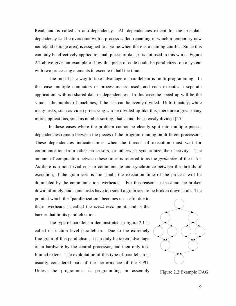
Figure 2.2:Example DAG
Read, and is called an anti-dependency. All dependencies except for the true data
dependency can be overcome with a process called renaming in which a temporary new
name(and storage area) is assigned to a value when there is a naming conflict. Since this
can only be effectively applied to small pieces of data, it is not used in this work. Figure
2.2 above gives an example of how this piece of code could be parallelized on a system
with two processing elements to execute in half the time.
The most basic way to take advantage of parallelism is multi-programming. In
this case multiple computers or processors are used, and each executes a separate
application, with no shared data or dependencies. In this case the speed up will be the
same as the number of machines, if the task can be evenly divided. Unfortunately, while
many tasks, such as video processing can be divided up like this, there are a great many
more applications, such as number sorting, that cannot be so easily divided [25].
In these cases where the problem cannot be cleanly split into multiple pieces,
dependencies remain between the pieces of the program running on different processors.
These dependencies indicate times when the threads of execution must wait for
communication from other processors, or otherwise synchronize their activity. The
amount of computation between these times is referred to as the grain size of the tasks.
As there is a non-trivial cost to communicate and synchronize between the threads of
execution, if the grain size is too small, the execution time of the process will be
dominated by the communication overheads. For this reason, tasks cannot be broken
down infinitely, and some tasks have too small a grain size to be broken down at all. The
point at which the “parallelization” becomes un-useful due to
these overheads is called the break-even point, and is the
barrier that limits parallelization.
The type of parallelism demonstrated in figure 2.1 is
called instruction level parallelism. Due to the extremely
fine grain of this parallelism, it can only be taken advantage
of in hardware by the central processor, and then only to a
limited extent. The exploitation of this type of parallelism is
usually considered part of the performance of the CPU.
Unless the programmer is programming in assembly

10
language, the optimizations imposed by a compiler will minimize the impact of the
programmer on the instruction level parallelism. For this reason most discussions of
parallelism in modern computers instead focuses on thread level parallelism, the
parallelisms between two or more streams of instructions.
In order to simplify the analysis of a parallel execution system, it is a common
practice to treat each “grain” as a separate object, and assume that any communication
occurs either at the beginning or end of the grain. As shown in figure 2.2, these grains
can be arranged into a directed acyclic graph (DAG) with the nodes representing
computation, and the edges representing communication.
For more information on parallel processing, [22] is a comprehensive text on the
subject. For an overview of how MHC uses parallelism see Chapter 5.
2.1.2 Heterogeneous Computing
Heterogeneous Computing (HC) is the practice of using computers with different
methods of computation to solve a single problem [9,1]. The practice arises out of the
observation that different types of processors are good at different types of problems. By
breaking a problem down into sub problems of different types, the time required to solve
the problem can be reduced if each piece is placed on the appropriate hardware. For
example, a task such as face recognition using support vector machines (SVM) can be
broken down into subtasks with different characteristics. In this example, the task can be
broken down into image segmentation, candidate selection, and SVM application. The
SVM part of this task, as the name would suggest, would perform much more quickly on
a vector machine than on a generic computer, while the candidate selection may run
faster on a high performance scalar machine. In a facility including both a vector
computer and a high-speed scalar machine, computation time can be reduced by
performing the SVM calculations on the vector machine and candidate selection on the
scalar machine.
HC has many of the same limitation as parallel computing above, and in fact uses
many of the same principles. The dependencies between the different pieces of the
problem have to be known, and the communication costs between the different computers
still limits the grain size to which a problem can be broken down [9].

11
Heterogeneous computing is usually applied in computing centers, which have
several different types of supercomputer on hand. In these environments, time and
money are closely linked, as the time over which an application runs is proportional to
the power consumption and the maintenance required. The motivation for HC in these
environments is to place the parts of a problem on the machines that minimize execution
time and monetary or energy cost.
The task of breaking up problems, and deciding on which machine they would
execute was originally done by hand, but there are now a wide variety of ways in which
to automate the process. Choosing a machine is known as matching, and choosing when
it is run is known as scheduling. These two choices are usually made concurrently and
called mapping collectively. Mapping algorithms are divided into two groups, those
which perform all the scheduling and mapping before any tasks are run, which is known a
offline scheduling, and those that perform the mapping while the processes are running
are known as dynamic or on-line schedulers[3,8,9].
The mapping requires information on which parts of the application will perform
best on each machine. In order to obtain this information analytical benchmarking and
code profiling are used to determine which type of computation is needed by each part of
the application, and how well each machine performs on each type of code.
Once this information is obtained, the required computation can be mapped by any
of a variety of automated schedulers. In all cases, a DAG is constructed of some or all
computations that have to be performed, and used to determine the order in which tasks
can execute. If a task were to be scheduled before a task it depends on, it is likely that
the system would give incorrect results or deadlock, depending on if the synchronization
between the tasks is enforced.

12
2.1.3 Linux Kernel Basics
Linux, the operating system on which this framework was implemented, was
chosen due to its open source nature, which allows it to be modified. To maximize the
effectiveness of MHC, the device queues and final scheduling stages must exist within
the kernel, or basic operating system, in order to be easily shared by multiple processes
and have direct access to the hardware.
Under Linux, all direct hardware access is accomplished by device drivers linked
into the kernel. User processes access these device drivers by connecting to special files
that represent the underlying device drivers. By implementing part of the MHC
framework as a device driver, a single point of access can be created, and a uniform
interface can be created to the individual device drivers [7].
One feature of the Linux kernel is that it is monolithic, meaning that all code
loaded into the kernel and data in the kernel share a single memory space. This indicates
that great care must be taken when adding a device driver to the system, as any small
error has the potential to bring down the entire kernel, at the very least causing the
machine to become unusable, and conceivably damaging the underlying hardware in the
worst case. As any errors in the kernel have a tendency to erase any log of the errors,
minimizing the changes and code used in the kernel is important to simplify the
debugging and reduce the chance of catastrophic errors.
Another reason for minimizing the amount of the framework that resides within
the kernel is the limited availability of kernel memory space, and the fact that the kernel
is not paged. This means that any memory used in the kernel is denied to other processes
on the system.
The Linux kernel is also constantly in flux, to the point that a piece of code
developed for one version of the kernel cannot be loaded, or in many cases even
compiled for the new version without changes that can vary from a minor change in a
make file to a complete alteration of interface. For this reason a specific version of the
Linux kernel, 2.4.2, was chosen as a target for this work.
13
2.2 Micro-Heterogeneous Computing General Concepts
2.2.1 The original vision
Micro-Heterogenous computing is basically a mechanism to allow the benefits of
heterogeneous computers to be applied on a smaller scale. Instead of separate
supercomputers connected by networks, MHC envisions a single computer, with several,
much more limited computational elements inside of it which vary in mode of
computation and capacity [8,9].
One of the primary goals of MHC is to reach smaller grain sizes than available in
traditional HC by reducing the distance between these components and connecting them
together with the faster internal interconnects available to modern personal computers
and servers.
MHC goes beyond merely improving performance as well. It also specifies that
the mapping of processes will be dynamic and automatic, and that the underlying
technology and hardware be transparent to the end user of the system, and the application
writer. This support for transparency even goes so far as to specify that the application
writer can provide serial code, and the MHC framework will execute it in a parallel
manner, extracting parallelism at the level of individual function calls.
In general, the task decomposition (breaking the application down into smaller
problems) is performed by the user when they select which functions to call. The MHC
framework must then re-order and schedule these tasks onto the available hardware in a
way that will ensure correct results, and hopefully a high speedup.
2.2.2 Meeting the Goals
This Micro-Heterogeneous environment as envisioned in [9] needs many
components to reach its diverse goals:
The goal of reaching a smaller grain sizes and maximizing performance requires a
high speed scheduling and mapping heuristic, capable of effectively and efficiently
placing tasks on devices with a minimum of overhead. To support this scheduler,
Analytical Benchmarking and Code profiling are done away with and replaced with

14
libraries of commonly used functions, each of which has known execution characteristics
on each device that supports it [8,9].
As these devices may need to be reconfigured for different function calls, or
between calls from different function libraries, there must exist a part of the MHC
framework that is capable of managing these configurations, and scheduling
configuration changes along with tasks. As some devices, such as FPGA’s may have
long configuration times, minimizing the number of configurations will be important to
overall performance.
In order to meet the goals of automatic parallelization, a component is needed to
analyze the tasks requested and find the data dependencies between them. This
component has to be able to track multiple in-flight tasks, and be able to dynamically add
and remove tasks from a DAG in order to determine which tasks can be scheduled at any
given time. Once again, this analysis is time critical, and must occur in a minimum of
time. More importantly, this parallelization cannot interfere with the ability of the
application writer to debug their programs; to meet this requirement, a novel error
handling method needs to be developed.
Even if these components function perfectly and make the MHC framework fast
and transparent, the system will still not be used if there is not a well-defined interface
that makes it easy for devices and function libraries to be implemented into the system.
This interface should be simple but flexible, with a variety of support functions to allow
beginners to access the framework along side experts.
All of these components are created and integrated in this thesis to provide a
functional MHC framework. In the coming chapters the implementations of these
components, and their sub components are discussed in detail. The entire system shown
in figure 2.3 is implemented in this thesis lacking only function libraries and actual
devices with which to work.

15
2.3 Implementation Overview
The system realized in this thesis in an implementation of the following ideal model:
One or more user applications request tasks in serial order from the MHC
framework. The MHC framework places these tasks into a series of queues, each
of which corresponds to a device capable of executing that particular task. The
placement of the tasks in the queues is done in such a way as to guarantee that the
results of execution will be the same as if they were executed in the serial order
they arrived in. The framework also makes an attempt to minimize the overall
execution time of all tasks it has so far received.
The way in which this is implemented corresponds to Figure 2.3: System Model
Overview shown below on the next page. The system was designed with the design
guidelines of modifying the kernel as little as possible, and allowing users as much
choice, or as much automation as they would like. These guidelines reduce the likelihood
that MHC will introduce instability into the system, while maximizing the utility to the
user.
The system implemented has several major parts: The function libraries, which
provide the user with pre-made MHC tasks; the dependency analyzer which allow
previously serial programs to take advantage of multiple processing elements
concurrently; the automatic mapping systems; and the device queues.
As the figure 2.3 illustrates, the function libraries, device configuration libraries,
automatic dependency analysis, and callbacks are all in user-space, allowing them to be
more complicated than implementation in kernel space would allow.
Chapter 6 explains the scheduling and mapping algorithms, which are divided into
two parts, the online scheduler and the batch scheduler. This allows the final, simplest
stage of scheduling to take place inside the kernel, where it can take into account the
behavior of multiple devices and has real-time status information about the devices, while
leaving part of the scheduler where it can implement complicated algorithms or be
customized by the user. The Schedulers used in this implementation of MHC ignore all
other cost metrics, such as power consumption, in order to focus on execution time.

16
User Code
Function Library
Base Library
Worker Threads
Software
ImplementationWrapper Code
Device Code Library
Device
ConfigurationsETC Prediction
Function Calls
Task Monitor
Construction
Tasks
Dependency Analyzer
Device
Configuration
Cache
DAGMemory
MapTaskReady To Run
Parameter
Requests
Batch Scheduler
Tasks Waiting To Run
Scheduled
Tasks
Kernel Space
User Spaceioctl
Online Scheduler
Software Queue
Tasks
Scheduled
To CPU
Device Driver Device Driver Device Driver Device Driver
Device Configuration Device Status
and Statistics
Gathering
Device Queues
Figure 2.3: System Model Overview

17
Chapter 3:
3 MHC Hardware
3.1 Classification
MHC compliant hardware could come in many forms. The actual requirements for
the hardware to work with MHC are actually fairly loose. To work with MHC, a piece of
hardware needs only three things: a connection to main memory or the CPU, the capacity
to carry out some useful computation, and a provision to allow the OS to limit the
memory ranges accessed by the device. Of course, it is desired to have devices that are
closely connected by high speed links, and which can perform a variety of tasks faster
than the general purpose processors of the system.
The following subsections discuss ways in which MHC compatible devices can be
classified, and how the different choices affect the utilization of the device by MHC.
Some of this material was originally presented in [9]. Because MHC uses a shared
memory assumption, and all operands are written back to main memory after a task, it is
especially hindered by communication costs. Several ways to improve this are
recommended in Chapter 10.
3.1.1 Embeddedness
The embeddedness of the device refers to how it is connected to the system, is
closely related to the latencies inherent in using the device. As discussed in section 8.1,
the effective minimum grain size of the system is determined by the scheduling
overheads and the computation to communication ratio on each device in the system. As
in any parallel processing environment, the higher the communication cost to the device,
the larger the grain size needed to break even or see a speedup. Also, the scheduling
heuristics used by MHC depend on the immediate availability of state information about
the various devices in the system, so the level of embeddedness is one of the most
important metrics of an MHC device. Network connected devices would be the most
distant device usable by MHC. These devices will tend to have high latencies, and
relatively low transfer rates. Devices connected in this fashion are not particularly

18
embedded, and are generally not considered effective for MHC. If the system consisted
solely of the CPU and devices connected in this manner, it would effectively be a
traditional heterogeneous computing environment with centralized scheduling and
messaging, which would not be very effective against other heterogeneous setups.
Connections over external peripheral busses such as USB, Firewire or fiber-channel also
fall into this grouping. The communication cost to computation ratios in this group are
generally several thousand to one for tasks with linear complexity, necessitating very
large grain sizes, and usually limiting it to high complexity tasks. Latencies for
communication to devices connected in this manner are usually measured in terms of
microseconds.
Devices connected to the internal peripheral interconnect such as PCI are the most
“distant” devices usually considered for MHC. Especially with newer standards such as
HyperTransport or PCI express, these devices are an order of magnitude better than
network attached devices. Direct memory access (DMA) protocols allow operands to be
obtained relatively quickly. The cost to access memory is usually within one (or in the
case of the aging PCI standard) two orders of magnitude higher than that experienced by
the CPU, allowing smaller grain size than with network attached storage, but still
effectively ruling out linear complexity tasks such as vector arithmetic. The cost of
memory access at this level varies from tens of nanoseconds for the newer interfaces to
about a half microsecond for the older interfaces.
Figure 3.1: Example PCI bases MHC system [9]
The next level of embeddedness is for the device to be connected to what is generally
called the north bridge. This would allow memory access rates nearly identical to those

19
experienced by the CPU, and enable linear task complexity to show a definite speedup.
There are not any industry standard connection busses for this at the consumer level.
Although some manufactures connect hardware such as integrated video controllers and
sound controllers at this level using proprietary interfaces, they still do not generally
grant them the same access speed as the CPU to memory. Using an as of yet
hypothetical connection to the north-bridge could give memory access latencies of a few
tens of nanoseconds.
Connecting higher in the memory hierarchy, the device may be integrated into the
CPU package in order to share level 3, or possibly even level 2 cache, enabling very
small grain size. These could expect memory access times on par with the CPU.
Special purpose devices at the functional unit level, or sharing level 1 cache, are
generally so well integrated that the scheduling cost of MHC would overwhelm their
ability to utilize extremely small grain size, and so would generally be controlled by more
specific mechanisms, most likely by a compile time or other static method.
3.1.2 Methods of Memory Access
The way in which a device will obtain the data it is assigned to work on will also
differentiate the device from others and affect its performance. Several possible methods
are contrasted below.
Perhaps the simplest method of data communication is register writes from the CPU
of the system. This method has several drawbacks, among them the fact that it is slow
compared to the other methods, and it ties up the central processing unit. This does not
disqualify this method from use by an MHC device, but it would limit it to jobs of very
high complexity.
Direct Memory Access (DMA) is one of the most popular methods of data transfer,
It is high speed and minimizes CPU utilization during the transfer. Some DMA methods
use user space IO, wherein they lock memory and transfer the data without the latency of
copying the data to the kernel. DMA access methods can be broken into two types, those
initiated by the driver running on the CPU, and those initiated by the device on an as-
needed basis. Transfers initiated by the driver have two advantages: validating the

20
memory range against the allowed memory regions is easy, and the duration for which
memory must be locked is well known.
On demand DMA transfers allow devices with limited onboard memory to more
efficiently process large jobs. However, transfers initiated by the device require a
hardware mechanism to prevent erroneous accesses and keep track of the physical
addresses of each page. In addition to this it will require the memory be locked for the
duration of the processing, or for the system page table to be kept synchronized with the
devices’ page tables, with a mechanism for handling page faults from devices other than
the CPU.
Devices attached high in the memory hierarchy can use either DMA to copy the
information from main memory to their local memory or access memory directly as
needed. If memory is accessed directly, the device will need the same level of paging
support as discussed above, as well as enough cache to support the burst rate of the
system it is interfaced to. This has the benefit of not requiring large amounts of onboard
memory on the device to process large data sets. Onboard memory may not be required
at all if the driver has provisions for allocating working memory areas in main memory.
The disadvantage to that approach is that the memory bus may become saturated if many
devices are present, and eliminate the benefits.
3.1.3 Types of MHC enabled devices.
MHC can encompass a wide variety of devices. A small number of the
possibilities which are available now are given here.
Field Programmable Gate Arrays, and other reconfigurable computing devices
have great promise for providing speedup. They are also extremely flexible . Any such
devices used in MHC should be reconfigurable when online, and have non-reconfigurable
hardware for bus interfacing. The capability for reconfiguration reduces the need for
additional special purpose processors (in cases where high concurrency between special
purpose devices is not needed), but the cost of reconfiguration is an issue.
Digital Signal Processors can show a decent speedup for specific functions such
as FFT’s and matrix multiplication. Also, many are available with a much better

21
computation to power ratio than the CPU, making it feasible to use DSPs multiple within
a single system.
Graphics Process Units or GPU’s are the most common embedded
heterogeneous processing platform. Almost every computer produced has one of these
special purpose processors optimized for texture generations and vertex transforms.
These operations use much of the same math as scientific applications, and there are
some projects being undertaken to retask these devices for scientific computing [23].
These benefit from faster busses, such as AGP and PCI express, which are made
available even on very cheap hardware.

22
Chapter 4: 4 Component Interfacing
4.1 Overview
The MHC framework is meant to interact with components from a variety of
sources. These parts include individual device drivers, function libraries, the kernel
module, the base library, and of course the user application. A well-defined interface
between each of these parts is a must to allow for extensibility and user adoption.
In designing these interfaces, the following goals were kept in mind. It should not
be necessary to know or use the entire interface to interact with the system. Knowledge
of only a small subset of the interface should be sufficient to gain most of the benefits of
the framework. The interfaces should be as flexible as possible, allowing the user to
access the system in different ways depending on their level of familiarity. In addition to
these considerations, the way in which the interface will influence performance must be
taken into account. A balance must be found between features available to the user and
the performance of the system.
4.2 Data Parameterization Method
In communicating with each other, the various components present in an MHC
application need a standard way to describe the data being passed by functions. As MHC
allows for automatic parallelization, the method of passing data must be sufficiently
introspective. In order to allow this, the passed data has to be parameterized to allow for
dependency analysis. This parameterization also allows for a single implementation of a
function to have the option of supporting multiple data types.
Each parameter passed to a function supported by MHC is assumed to be
contained in a contiguous region of flat memory (the memory uses no position dependent
information such as pointers), composed of a number of homogeneous elements, each of
which is 4 kilobytes or less in size. Larger data elements can be handled by treating them

23
as a character array. The reason for the limitation to flat memory regions is discussed in
Chapter 5.
Parameters are passed to the MHC tasks as an array of parameter structures. Each
parameter structure contains the following information: The type of the operand and the
size of the type, the size of the memory region, in multiples of the operand size, whether
the operand is an input or an output, and finally, either the data value itself or a pointer to
the data value. The C style structure is shown below in Figure 4.1: MHCParameter Data
Structure. typedef struct { unsigned long long data; unsigned long type; unsigned long size; }MHCParameter;
Figure 4.1: MHCParameter Data Structure
The data member is either a pointer to the operand, or the operand itself. In the
case of pointers or data less than 64 bits (referred to as an immediate value), the data is
aligned to the lower bytes in memory order, as if a pointer case where performed. The
macro PARAM_TO_TYPE is provided to simplify this process.
The type field is broken down into a number of bit fields, as shown below.
Bit Range Description 31~30 Read/Write mode. These bits are used to determine how the device is used
when dependency analysis is called for, or errors must be propagated. Bit 31 indicates that this parameter is treated as an input and will be read. Bit 30 indicates that the parameter is an output and will be written. Both bits must be zero if the parameter is immediate.
29~25 Bits 29~25: Library Designator. These bits divide the data values into classes. Currently a value of 0 means standard C types, and a value of 0x1E indicates user defined data types. All other values are reserved for future expansion.
24~12 These bits are used to arbitrarily assign values to different types. Two types may not share an identifier.
11~0 Size per element. These bits indicate the size of the type per element in bits.
Table 4.2:Parameter Type Bit Fields

24
The size field indicates the multiplicity of the data. If the value is 0, the parameter
is immediate, and the value is stored in the data field. Any other value indicates the
number of data elements at the location in memory indicated.
4.3 Task Representation
The representation of a task in the system by necessity differs slightly between the
kernel and the user space. In each case, a common representation of the task is encased
in a wrapper structure that stores the extra information necessary to for the different
representations.
The basic representation of a task in the MHC framework is the MHCTask data
structure. In order to prevent optional features from unduly slowing down those tasks not
using those features, pointer fields are used in the structure to indicate which extra
features are used and the location of the pertinent data. The structure is shown below in
figure 4.3, and the data members of note are described in Table 4.4: MHCTask member
description.
typedef struct mhc_task {
unsigned long ID; unsigned long deviceID; unsigned long ETC; unsigned long long EST; unsigned long flags;
MHCCode * code; int numParams; MHCParameter * params;
MHCSchedulerParams * sParams;
char codeID[32]; //not used by user-space programs int command;
};
Figure 4.3: Task Representation

25
Field Description
ID The ID field is used as output passed to the user task, and is used to perform operations altering the state of the task after it is submitted to the kernel.
deviceID The device ID is used to indicate the device on which the code will execute. If the automatic device selection is enabled, this is an output from the kernel to user space. Otherwise it is provided by user space.
ETC EST The Estimated Time to Completion and Estimated Start Time fields are used to indicate the predicted computation time and start time of the task. EST is always provided by the kernel, but ETC can be provided by either the kernel or user space.
Flags The flags variable indicates how the task should be treated by the kernel scheduler. Currently the only user defined flags are MHC_HOLD, which will cause the task to be scheduled, but not executed when it reaches the head of the queue; and MHC_PARANOID_CODE, which forces the device configuration to be reloaded if it was previously loaded by a different process.
Code The code pointer points to the user space location of the code used by this task. The Id string of this code is repeated in the codeID field to reduce the cost of determining reconfiguration latencies. The command field is used to select one function out of the many possible with any given device configuration. See the next section
params numParams
Params is a pointer to an array of numParams parameters as described above in the parameterization chapter..
sParams The sParams structure is used by the online scheduler, and is described in section 6.3:Online Scheduler. This field supercedes the deviceID, ETC, code, and command variable when not null
codeID This field is used internally by the kernel to track the configuration assigned to a task.
command The command data member is used to specify what sub function of the configuration provided is to be used.
Table 4.4: MHCTask member description.
4.4 Device Configuration Representation
Each device configuration is stored in a flat region of memory, and is identified
with a unique identifier similar to that used in Java package names, in a format
“tld.organization.device.code_identifier”. This identifier need only be unique with
respect to other installed devices for the system to function, but for human readability
reasons it is desirable for it to be globally unique. This is limited to 31 characters, not

26
counting the terminating null common to all C strings. For instance a piece of code from
a fictional “dumbycorp” used to compute the FFT on a device known as the x235a may
have an identifier “com.dumbycorp.x235a.fft.”
Each configuration starts with a header as shown below in Figure 4.5: Device
Configuration Header. This structure describes the configuration in enough detail for
MHC to get the correct configuration to a device. The remainder of the memory region is
specific to the device to be configured, and is merely passed along by MHC. Table 4.6
explains the utility of each field.
struct mhc_code {
char codeID[32]; unsigned long code_type; unsigned long typeMajor;
unsigned long typeMinor;
unsigned long size; unsigned long flags; int scriptOffset; };
Figure 4.5: Device Configuration Header
Field Description
codeID Contains the code identifier, as described above. code_type This field is used to check compatibility of the code with the device. It
must match the code_type of the device exactly. typeMajor This field is used to check compatibility of the code with the device. It
must match the typeMajor of the device exactly. typeMinor This is used to check compatibility with a device. This field consists of
32 flags whose meaning is device defined, and indicate variability between compatible devices.
size This field indicates the size of the data following the header. flags These are device dependant flags indicating special treatment.
scriptOffset This field is used by drivers that, in addition to configuring the device, execute a script to transfer data or provide other functionality. The meaning of this variable is intended to be the location in the data where the script begins, but in practice is defined by the driver.
Table 4.6: Configuration Header Description

27
4.5 Driver Interface
Without device drivers for various devices, MHC becomes nothing more than a
fancy way of ordering thread execution. In order to encourage the support for MHC, the
driver interface has been kept to the minimum set of functionality necessary to support
the system. As much flexibility as possible is left to the driver writer in terms of
decisions on memory access and timing.
There is one important limitation imposed by the structure of the Linux kernel. In
order to transfer data to or from a process, the processes must be the current context, or
have a locked memory region. As the tasks submitted from user space will sit in a queue
before being dispatched, it is not guaranteed that the context when the task is chosen to
run will be the same as the context when the task was submitted.
There are three solutions to this problem, each with drawbacks and limitations.
These are described below.
The first and most obvious solution is to copy the data in question to kernel space
when the task is requested. This has several drawbacks, among them: Kernel memory
space is precious, and in tight supply. As kernel memory is not paged, and shared by the
memory space of all running processes, any memory allocated to a kernel buffer is not
available to any other processes, and will increase the amount of paging in the system.
Also, using kernel buffers would place a variable upper limit on the total size of
parameters used anywhere in the system with MHC. As MHC tasks will most likely be
working with large data sets, this would not be conducive to making the system
transparent. This approach is also very wasteful, as it will essentially double the memory
requirements, and require that the memory be copied more than necessary.
The second method is near ideal, but was rejected due to limitations in 32 bit
Linux. It is possible to lock a memory region into physical memory and map the memory
into the kernel memory space. This solves the problems of copying memory, and high
inefficiency in the first solution, but shares the problems of excluding physical memory
from other applications, and the limitations of kernel memory space. On 64 bit systems,
with higher addressable RAM limitations and greater kernel memory space, this may
have been a more acceptable option.

28
The solution that was chosen requires each task to have a user level thread
associated with it that blocks while the task is queued. This has the benefit of simplifying
the coding in the kernel by allowing much of the task synchronization to be shifted to
user space. The downside is that after waiting in the queue, the task cannot execute until
the thread associated with it is once again scheduled by the primary Linux scheduler,
which could be a delay on the order of tens of milliseconds, depending on load. This can
be mitigated by elevating the thread to “real-time” status, while it is waiting in the queue.
This will give it priority over all regular long running tasks, but even best case will
introduce two additional context switches per task (one when it starts executing, and the
other when it stops).
Many devices currently have proprietary interfaces. Participation in the MHC
framework does not prohibit the use of the other interfaces, but does place the following
limits on it: Any use of the other interface may not take place while the queue for that
device contains jobs. The device can use the notify function (described below) to prevent
new jobs from being scheduled to the queue to facilitate emptying the queue. Also, if the
device is marked as exclusive in MHC, the device may not use its alternate interface with
any process except for that which has exclusive access.
4.5.1 Device Description and Status
Each device registered with MHC has to have a certain amount of information
associated with it so the correct code can be selected to run on the device. This
information is made available to the user application, and so is kept separate from data
used only by the kernel. The exposed information about a device is broken up into two
parts, information that describes the device, and information on the current state of the
device.

29
4.5.1.1 Device Description
The descriptive information about a device is described in the following structure:
struct mhc_device_descriptor { unsigned long code_type; unsigned long TypeMajor; unsigned long TypeMinor;
unsigned long performance; char manufacturer[32]; char description[32]; };
Figure 4.7: Device Description Structure
Field Description code_type identifies the family of code the device uses. TypeMajor the major type of the device, used to check the compatibility of code. TypeMinor A bit mask indicating optional features Performance the performance (in percent) relative to a baseline device used for ETC
calculations. Manufacturer the name of the manufacturer Description a human readable name that identifies the device, should be unique
within each manufacturer. This, along with the manufacturer name is used for automatic setup.
Table 4.8:Device Description Fields
For a piece of code to be compatible with a device, code_type and TypeMajor
must match exactly, and any TypeMinor bits set in the code structure must be set in the
device structure.

30
4.5.1.2 Status
There are many things which have to be tracked for each device in order for
scheduling to occur effectively, and to enable capabilities such as exclusive device
access. The status information kept on each device and judged to be useful to userspace
applications is stored in the following structure: struct mhc_device_status{ unsigned short ID; unsigned long flags; unsigned long long lastJob; pid_t exclusive; pid_t code_pid; char loadedCode[32]; unsigned long last_update; int dynamic[MAX_DYNAMIC]; };
Figure 4.9:Device Status Structure
Field Descrition ID the ID of the device assigned when it is registered with the MHC
framework Flags bit flags indicating how jobs will be scheduled to the device LastJob Indicates when the last job was scheduled on the device (not currently
used) Exclusive if non-zero, indicates the specified PID had been granted exclusive device
access, and no other processes can schedule new jobs on the device. Code_pid The pid of the process which loaded the code that is currently on the
device. Last_update indicates the last time (in jiffies) at which the dynamic scheduling
information was updated. Dynamic information used by the scheduling mechanisms. The data contained is
updated frequently and is described in section 6.2. The device should fill Dynamic[0] with the average configuration time of the device, if it is non trivial.
Table 4.10:Device Status Fields
4.5.2 Functions provided to the drivers
The kernel provides three functions for the use of the driver. The first of these
functions allows the driver to register with the kernel module. The second of these
functions allows the device to notify the kernel module of a change in state. The last
function unregisters the driver and cancels all outstanding jobs.

31
The registration function takes as a parameter a data structure describing the
device and another specifying the functions supported by that device. These functions
are described in the next section. When registering, the driver can specify the default
operating mode of the device, as well.
The notification function takes a integer indicating the type of notification and an
optional parameter. This function is only used when something happens asynchronously,
and can be ignored by devices that are not hot-swappable and do not support
asynchronous code loading. Access is also provided to the device array maintained by
the kernel driver, along with the spinlock used to protect it. The constants used for
notification are shown in Table 4.12:
MHC_CODE_CHANGE The code loaded on the device has changed asynchronously
MHC_DEVICE_UNAVAILABLE Indicates the device will be temporarily un-available. The queue is paused, and new jobs are still accepted.
MHC_DEVICE_ERROR An error occurred on the device and the current job is unrecoverable
MHC_DEVICE_GOING_DOWN The device will be unavailable to MHC at a known time in the future. The parameter indicates how long until the device goes down. No further jobs are accepted, and any current jobs that would run past that time are cancelled.
MHC_DEVICE_REMOVED The device has been removed from the system, all jobs must be cancelled immediately. If there was a currently executing job, it has already returned with an error.
Table 4.11: Supported Asynchronous Notification
32
4.5.3 Functions Provided by the Drivers
Most of the functionality of the system is done through a few functions provided by
a driver when it registers with the system. There is a minimal set of calls that must be
supported by the driver, and a set of optional calls. The minimal set is kept extremely
simple, in order to make converting devices to work with MHC as easy as possible.
At a bare minimum, the driver must provide a function to load a configuration or
code onto a device, start executing a job using the current configuration for the device
and a function to stop the execution of the code. All of the minimum set of functions are
called from a user context, with no locks held. This means that the driver has its choice
for how to handle memory transfers from user space, and can block or sleep until it
finishes.
The optional functionality for the driver encompasses asynchronously loading code
without blocking, and predicting configuration latencies. The specific functions the
driver may support are indicated in Table 4.14 below, as well as whether they are
optional or mandatory. Each function takes as its first parameter a number that identifies
the device on which it should act. The driver specifies this number when it registers the
device, and it is passed back to the driver whenever a function is called. This convention
allows a single driver to support and register any number of devices, within reason. Also,
each function returns a value. 0 indicates success, while a negative number indicates
failure, and will be returned to the user.

33
Function Description Parameters unsigned long device_ident
MHCCode * code – a pointer to code in user space
load_code Manditory
This function will synchronously load code to the device. It is always called from a user context.
int force – load the code even if code of a matching identifier is already loaded. unsigned long device_ident MHCCode * code – a pointer to code in kernel space. This will always be kfree()’ed by the driver.
async_load_code Optional For future expansion
This will asynchronously load code to a device, without blocking the calling thread. This load should cancel automatically on any other function being called on the device, and should culminate with the notify function being called.
int force – load the code even if code of a matching identifier is already loaded. unsigned long device_ident
char * name – the string identifying the configuration
estimate_load_time Optional
This function will estimate the time it will take to load the named code on the device
int force – if true, the code will need to be reloaded. unsigned long device_ident stop
Mandatory Cease execution of the current task, if any. Return –EPIPE. unsigned long flags – reserved for
future expansion, ignore. Set or read options on a device. unsigned long device_ident unsigned long option- which option to set. void * param – a pointer to what to set the option to,
or where to read it to. Int write – if true, write the option, otherwise read it.
option Optional For Future Expansion
Int userspace – if true, the pointer points to userspace. unsigned long device_ident MHCCode * code – a pointer to the configuration in userspace, this can optionally be used to verify that the correct configuration is loaded. MHCParameter *params – a pointer to an array describing the data to be used, as described above, in userspace. int numparams – the size of the params array.
start Mandatory
Execute a specific command with the passed data and configuration.
int command – the command to execute. By convention commands with negative values are special. So far only –1 is defined, and should result in start immediately returning 0.
Table 4.12: Functions provided by the driver

34
4.6 Kernel Interface
The interface between the kernel and user space will be one of the most used
interfaces of the framework, as it will most likely be used several times for each job
scheduled. The interface between the kernel module and user space is done exclusively
through Linux ioctl (input output control) calls. Although creating a custom system call
would have been slightly faster, doing so would require a consensus from the Linux
community and hinder adoption of MHC. Also, the use of ioctl calls is the accepted way
to expose functionality that does not meet the read/write paradigm used by most drivers.
4.6.1 ioctl overview
Ioctl calls in userspace take three arguments: a file descriptor, a command, and a
parameter. On the kernel side, the ioctl call provides the underlying “inode” and “struct
file” of the file passed from userspace, as well as the command and parameter from user
space. The kernel module creates a single device file, which acts as an entry point for all
user space programs wishing to use MHC to schedule tasks on devices. As each process
to open the device file receives a different “struct file” and then shares it with all of its
child threads, the MHC kernel module uses this “struct file” to determine whether a
thread has access rights to a particular task. Under a POSIX compliant system, this
would be done more elegantly based on process ID, but many versions of Linux still in
use are not fully compliant with the POSIX specification for thread.
For convenience, I have supplied a wrapper function for each ioctl command that
automates the process of calling it. As many of the commands require pointers to data
structures, the wrapper functions allocate and fill out the data structures for the user
before making the ioctl call. These wrapper functions are inlined and make use of the
stack to minimize their cost.
4.6.2 ioctl commands
This subsection describes the constants that are passed to the IOCTL system call
for each of the operations supported by the kernel module. Each constant has a particular
type of data, which the last parameter of the IOCTL call will be cast to. Normally, the
user will access these functions indirectly through the wrapper functions provided by the

35
base library. Although all user input is validated to the extent that it will not interfere
with the performance of the machine, it is still possible for the user to provide input (such
as requesting a read to the wrong address) that will cause that program to fail.

36
4.6.2.1 Commands Working With Devices
These commands allow the user to get information about and change the state of
devices attached to the system. In all cases it is the responsibility of the user to provide a
buffer to store the returned information.
Constant Description Parameter MHC_DEVICE_LIST This call will fill a buffer with the
description of all devices in the system.
MHCDeviceListRequest *
MHC_QUEUE_ENUM This call will fill a buffer with the task that are in the queue for a particular device. The information provided includes the PID,ETC, and flags of the tasks.
MHCQueueEnumRequest *
MHC_DEVICE_STATUS This call will fill an mhc_device_status structure with the current status of the requested device.
MHCDeviceStatusRequest *
MHC_REQUEST_EXCLUSIVE This will request exclusive access to a particular device. If granted, new tasks from other processes are prohibited from scheduling on this device. Normally only root can request exclusive access, but can make it globally available with MHC_SET_FLAGS, below.
unsigned int
MHC_RELEASE_EXCLUSIVE This will release a device which has been marked with exclusive access restrictions. Non-superuser processes can only release devices marked exclusive to them.
Unsigned int
MHC_SET_FLAGS This ioctl call is available to the superuser only, and allows the setting of flags that control the operation of the device. Flags that can be set include the application of reconfiguration latency hiding, and permissions for exclusive access.
MHCDeviceFlags *
Table 4.13: ioctl commands working with devices

37
4.6.2.2 Commands Working With Tasks
These commands are used to interact with tasks. All of these commands are
available to all processes. Users with superuser status can utilize some of these
commands on tasks not belonging to them, although to do so they have to know the
correct identifier.
Constant Description Parameter MHC_SUBMIT This command requests a
task be scheduled to a device queue.
MHCTask *
MHC_KILL_TASK This will request a task be cancelled and removed from the kernel module. The thread waiting for the task will return with –EPIPE. Non-superuser processes can only kill their own tasks.
MHCTaskIdent *
MHC_RELEASE_TASK This command will set a tasks hold flag to 0, allowing it to execute normally. Non-superuser processes can only release their own tasks.
MHCTaskIdent *
Table 4.14: ioctl commands working with tasks
4.6.2.3 Commands Working With Time
These commands are used to allow userspace to make sense of the timebase used
by the MHC kernel module.
Constant Description Parameter MHC_NOW This returns the current time as seen by
MHC unsigned long long *
MHC_HZ This returns the number of times per second the MHC timebase is incremented.
N/A
Table 4.15: ioctl commands working with time
4.7 Base Library Internal Interface
The base library has an internal interface intended for use by individual function
libraries in conjunction with the functionality available to the user. The functions

38
provided automate common tasks and greatly simplify the creation of a library that
conforms to the standard format. The functions include locating and parsing standard
files; Creating and Scheduling tasks; and the loading and caching of configuration data
for the devices.
4.7.1 Job Size Estimation
The system as currently implemented allows the library to estimate job size by up
to 3 dimensions. The dimensions are used to determine which implementations can be
used with a given task, and to calculate the estimated cost of execution on a particular
device. A four-term polynomial is used to approximate the execution time of each task.
A four term polynomial provides acceptable approximation of the cost functions over a
fixed range for many functions. Work recently completed in [14] demonstrated that for
many functions this approximation method works, although at a higher cost than other
methods such as multi-cord.
4.7.2 Standard File formats and Parsing
Each function library and device in the system is described by a file. These files
indicate the functions supported, and the conditions under which they can be used. These
files are kept in a well-organized directory structure so they can be easily found for
automatic configuration. Functions are correlated between the two files using the library
name, a string, and the integral function number.
The library description file is the simpler of the two files; it consists of a list of
function numbers, triviality values, and execution cost functions. In the library file, the
function number is unique, because the software fallback provided by the library must
support all job sizes. The triviality number indicates a job size, below which the cost to
execute the task in software is less than the cost to select a device to run a task.
The device file is somewhat more complicated than the library file. It is divided
into sections, each corresponding to a different library. Within each section is a list of
functions. In additions to the information listed per function in the library file, the
following information is contained on each row: a minimum and a maximum job size for
each of the three dimensions; required flags that have to be set in the device’s TypeMinor

39
Field; a set of flags that may allow a library to disqualify that implementation; and file,
offset, and size where the configuration information for the device can be found.
Each function number can be repeated multiple times. This allows for multiple
implementations that handle different sizes of jobs, use different optional features, or just
have different cost curves. This also allows for a single function with a cost function not
expressive in terms of the chosen estimation method to break the estimation up into
regions to improve accuracy.
For instance, a single device may support two different functions for calculating the
some transform on a set of data. The first, a very fast implementation, may only work on
small task sizes. The second implementation may have a cost execution function that is
not easily expressed in polynomial form, such as a logarithmic cost. In the device file,
these would be represented as multiple entries with the same function number. In this
example, three of these duplicate entries would exist: One for the first, fast
implementation; and two for the logarithmic cost implementation. By using two entries
for the logarithmic function, one entry can be used for the highly curved section of the
cost prediction function at low task sizes, while the other will be used for the linear
section at large task sizes.
The files containing configuration for the device all have a standard header
containing the MHCCode structure as described above for each piece of code in the file.
Currently, the standard requires this structure to be filled in using big endian byte order
(network order). Implementations should be sure to adjust the byte ordering
appropriately on loading the code for the MHCode structure, but not for the remainder of
the file, which consists of compiled code for the device.
The function provided by MHC to the base library will automatically parse these
files, if they are in the standard positions. For each library, it will create a list of
functions, and of devices that support the function and are available on the system at the
time the call was made.
4.7.3 Automatic Task Creation and Submission
When a function library requests a task be submitted, it provides the job size, the
function number, and a callback function in addition to the parameters for the function.

40
The method provided by the base library takes this information and for each device finds
the configuration that gives the lowest ETC. These are then used to fill a scheduler
parameter structure as described above. If the task’s size is smaller than the triviality
number for the function, the task is executed immediately on the GPP.
As this occurs, the function also sees to it that the configurations are loaded into
memory and will be removed from memory at an appropriate time. This is done by using
a callback to invoke the cache handling methods automatically when the task finishes.
Also, if the user has requested it, the dependency analyzer is invoked, as described below
in chapter 5. int LibAutoConfigure( MHCFLib* in, char * name ); void LibAutoCleanup( MHCFLib* in); int MHCLibAutoCall( MHCParameter * params, int numParams,
int function, MHCFLib* lib,
unsigned long size0, unsigned long size1, unsigned long size2, int (*callback)(int numParams,
MHCParameter* params ));
Figure 4.16: Base Library Functions Used by a Function Library
4.7.4 Loading and Caching of Configuration Data
The interface to the drivers described above requires that the configuration data be
present in the memory space of the requesting task at the time of submission. To make
this easier, the base library provides a set of methods that maintain a cache in memory of
the code which is needed at any given time. The cache keeps track of jobs in flight, and
uses reference counters to mark the code as unused when it is no longer needed.
Modern OS’s use virtual memory, and this mechanism can be relied upon to
provide the functionality provided by the cache in terms of managing what pages are
available in memory. The cache would be unnecessary but for the fact that because the
user code may not be aware of the number of MHC devices installed in the system, or the
size of a configuration for each of those devices, it is possible although not likely, that
calling multiple functions will result in the MHC framework requesting a larger amount
of memory than can be allocated in the virtual address space of 32 bit Linux systems.

41
The cache is not so much to manage physical RAM, but to manage the addressable
memory space.
The maximum amount of memory to dedicate to the cache is configurable by the
user, and defaults to 500MB, (one quarter the available memory space for a 32 bit Linux
process). To maintain transparency, if more memory is needed, the calling thread will
block until space in the cache becomes available. This may deadlock if tasks using very
large configurations are allowed to create other tasks. For this reason the callback for a
task is prohibited from creating additional tasks.
4.8 Base Library User Application Interface
The Interface provided to the applications is a superset of the functions provided by
the base library. It includes the wrapper functions to communicate directly to the kernel
module. Also provided are functions and global variables to control the operation of the
schedulers, methods to allow synchronization with tasks submitted to the system, and to
incorporate their own code into the system.
Most of these functions are most useful if all interaction with MHC takes place
from within one thread. In the interest of flexibility all of the functions provided to the
user are thread safe, unless otherwise noted.
4.8.1 Scheduler Configuration
A number of commands exist to control the way in which a set of tasks are
parallelized and scheduled. For cases where there are limits on the allowable settings, or
where settings can only be changed at certain times, a function has been provided to
change the settings in a safe way. In most cases, MHCJoin(0,0) should be called before
changing configurations.
The most important function that determines the operation of MHC is the
MHCMode function. This function allows four parameters to be set, as shown in table
Table 4.17: MHCMode Parameters. This function can only be called when there are no
jobs present in the system. If called and an inappropriate time or with bad values, it will
return an error. The default values result in serial execution with greedy scheduling.

42
The dependency analyzer described later has a function CheckOverlap, which
takes an integer controlling whether the O(1) (hash table) or O(log(n)) (binary tree)
dependency analyzer is used. If the O(1) analyzer is used, parameters must either match
completely or not overlap at all. This function can only be called when no jobs are in the
system. int TaskSubmitAsync( MHCTask * in, TaskMonitor ** monitor ); void CheckOverlap( int i );
Parameter Permissible Values Description Parallelize On/Off ( 1/0 ) Whether tasks submitted
should be executed serially or parallelly
Dependency Analyzer On/Off (1/0 ) Whether the automatic dependency analyzer should be invoked. Requires Parallelization on
Online Scheduler 0~MAX_SCHEDULERS-1 Controls the coefficients used in the minimization process to select a device to run a job.
Offline Scheduler 0 – off Pointer to a Batch Scheduler
Controls the offline scheduler, see section 6.4 for details. May Require the dependency analyzer.
Table 4.17: MHCMode Parameters
Global Variables are provided to control the maximum number of CPUs used for
the execution of callbacks (gNumCPUs) and the amount of memory used by the caching
system (gMaxCacheSize). These values can be changed at any time, but if they are
reduced the system will not actually reduce the corresponding utilization immediately.
4.8.2 Functions working with submitted tasks.
Many functions are provided to allow the user to get information about a submitted
task, or to synchronize with tasks already in the system. In an effort to allow maximum

43
functionality, many functions serve similar purposes or do the same thing in different
ways.
There is a large amount of data available in the task monitor structure about
submitted tasks. The user can peruse the data, but if any of the structured data associated
with the task monitor must be traversed ( such as the DAG, or the dependency lists) they
should lock the mutex associated with any task monitors accessed to prevent it from
being de-allocated or altered until the traversal is complete..
4.8.2.1 Obtaining a Task Monitor
The main way the user interacts with the submitted tasks is the use of the task
monitor structure, so the user should use the correct functions to handle the reference
counts, shown below: void TaskMonitorRef( TaskMonitor * in ); void TaskMonitorDeref( TaskMonitor * in ); void GetNextTaskMonitor( TaskMonitor ** mon );
To get the initial reference to a task monitor, a function is provided to get the task
monitor for a job which is automatically submitted by a function library. By invoking
GetNextTaskMonitor(), the user can request a reference to the next task submitted by the
current thread. The reference count of the task is incremented, so the user should
dereference it when they are done with it.
4.8.2.2 Waiting for a Task to Finish
The user can wait for a task to finish in one of three ways. They can wait for all
tasks to finish, wait for a particular range of memory to become available, or wait for a
specific task to finish.
Waiting for a range of memory is done with MHCJoin(). If dependency analysis
is on, the user specifies the start and stop of the memory range on which they wish to
wait, or 0 if they wish to wait for all memory ranges.
Waiting for a specific task is done with the TaskMonitorJoin() function. A
specific task monitor can be specified, or NULL can be passed to indicate all jobs should
be completed before it returns. The prototypes for these functions are:
int TaskMonitorJoin( TaskMonitor * in ); int MHCJoin( void * start, void *stop);

44
Figure 4.18: Functions that wait for tasks to complete.
4.8.2.3 Performing Operations After A Task Completes
Under some circumstances, such as when the user is using their own dependency
handling scheme, it is necessary to have some piece of code run after a task has
completed without blocking as happens when one waits for the task to finish.
For this reason a function has been provided that will allow the user to run a
function immediately upon the completion of a task. This function takes a generic
callback function, taking a single pointer and the task that has just finished as arguments.
The only limit on the behavior of this callback is that it cannot lock the mutex of the task,
and it cannot call pthread_exit. The thread the callback is executed from will hold the
mutex on the task finishing. The way in which this is implemented allows the user to
register several callbacks, which will all run on the completion of the task. The order in
which they are run is not specified.
The function used to install this callback is shown below:
int TaskCallOnFinish(
TaskMonitor * mon, void (*callback)( void * data, TaskMonitor * mon), void* data );
Figure 4.19:Task Call On Finish Structure
4.8.3 Submitting User Code to The system
4.8.3.1 Submitting a user defined task
If the user wishes to create a task that is not available in any function library, the
mechanism is a bit complex, but in the spirit of severability, it is allowed. The user
provides one or more of the following:
• A software implementation of the task.
• One or more implementations for specific hardware.
The user then fills out a scheduling parameters data structure, a parameter data
structure, and the task data structure. The function shown below is then run. “in” is the
task structure filled out by the user. “monitor” is an optional output of the task monitor
created. “callback” is the software callback to be run if the task is not scheduled to a

45
device. “cleanup” is a callback that is executed after the task has completed, regardless
of success or failure.
int TaskSubmitLib( MHCTask * in, TaskMonitor ** monitor, int (*callback)(int numParams,
MHCParameter* params ), void * data, int (*cleanup)( void *data ) );
Figure 4.20: TaskSubmitLib function call.
4.8.3.2 Submitting a callback only piece of code.
Occasionally a user of MHC way wish to execute some function on data written
by an MHC task, but using one of the synchronization functions described above would
serialize the system to an undesired degree. In these cases the user can submit a callback
to the MHC framework, and have it dependency checked and run as if it where a standard
task.
This is done using the function shown below. As with any code handled by the
MHC framework, the parameters to the task have to be described using the
MHCParameter structure. If the user wishes to obtain a task monitor reference, they can
pass a pointer to the location they would like the pointer to the task monitor to be stored.
There are some limits on the behavior of a callback. Most notably, the callback should
not create more tasks. More details about the implementation and its uses are available in
chapter 5. int CallBackSubmit(
int (*callback)(int numParams, MHCParameter* params ),
int numParams, MHCParameter* params , TaskMonitor ** mon);
Figure 4.21: Callback Submission Function.

46
4.9 User/Function Library Interface
4.9.1 General Conventions
4.9.1.1 Parameter Sources
When a user is using MHC through a function library they must keep in mind the
limits of the dependency analyzer. Because the dependency analyzer can only analyze
those parameters passed by pointer, the following convention should be followed:
If the parameter is passed by pointer, it takes part in dependency analysis. If it is
passed by value, it is not considered for dependency analysis (because the address cannot
be known ) and must be less than 64 bits. This means, among other things, that if a
parameter passed by value is an output from a previous MHC task, the user cannot
request the task using it until the task producing it has finished. This can be guaranteed
using one of the MHCJoin functions.
4.9.1.2 Return Values
All function library functions should return only error codes. As the function
may be executed asynchronously, the results or the task will not be available
immediately. In the cases where the function is modeled after the function in another
library with a return value, the return will instead occur to a memory location pointed to
by the last regular parameter, and will be called retval.
4.9.1.3 Function Naming
All functions coming from an MHC function library will begin with mhc_<library
name>_ or mhcd_<library name>_. For instance the functions coming from the gsl
library will begin with mhc_gsl. This was chosen to make converting an application
from an existing library to a MHC compliant function library simpler. It also prevents
confusion over duplicate function names in different libraries.
If mhcd_ is used, the function supports one additional parameter per regular
parameter, of the type unsigned long. These additional parameters can have the value of
MHC_DEP_CHECK or 0, and are not passed to MHC, but are instead used to suppress
the dependency checking for one of the other parameters. Although it is not required that
a function library provide this, it is recommended for all functions with a large number of

47
parameters. In these cases allowing the user to specify which parameters they know do
not have dependencies can reduce the overhead of building the DAG.
The code segments shown below illustrate the process of creating a wrapper for a
function library. Figure Figure 4.22: Original gsl_blas function shows the original code
from the gsl_blas library. Figure 4.23: Example Function Library Wrapper shows the
wrapper implementation from the mhc_gsl_blas library. Note that the original library
call has been used as the callback for the MHC code, and that the input validation takes
place before the call is submitted to MHC.
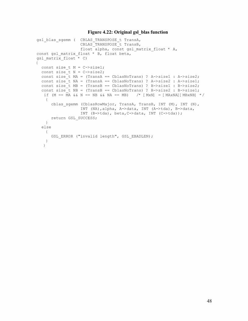
48
Figure 4.22: Original gsl_blas function gsl_blas_sgemm ( CBLAS_TRANSPOSE_t TransA,
CBLAS_TRANSPOSE_t TransB, float alpha, const gsl_matrix_float * A,
const gsl_matrix_float * B, float beta, gsl_matrix_float * C) { const size_t M = C->size1; const size_t N = C->size2; const size_t MA = (TransA == CblasNoTrans) ? A->size1 : A->size2; const size_t NA = (TransA == CblasNoTrans) ? A->size2 : A->size1; const size_t MB = (TransB == CblasNoTrans) ? B->size1 : B->size2; const size_t NB = (TransB == CblasNoTrans) ? B->size2 : B->size1; if (M == MA && N == NB && NA == MB) /* [MxN] = [MAxNA][MBxNB] */ { cblas_sgemm (CblasRowMajor, TransA, TransB, INT (M), INT (N), INT (NA),alpha, A->data, INT (A->tda), B->data,
INT (B->tda), beta,C->data, INT (C->tda)); return GSL_SUCCESS; } else { GSL_ERROR ("invalid length", GSL_EBADLEN); } }

49
Figure 4.23: Example Function Library Wrapper
( 1 of 2 pages ) //function number in function library #define MHC_GSL_BLAS_SGEMM 1234 //Callback Function static int gsl_blas_sgemm_cb( int numParams,
MHCParameter* params) { cblas_sgemm (CblasRowMajor, PARAM_TO_TYPE( params[0],int ), //TransA, PARAM_TO_TYPE( params[1],int ), //TransB, PARAM_TO_TYPE( params[3],size_t), //INT (M), PARAM_TO_TYPE( params[4],size_t), //INT (N), PARAM_TO_TYPE( params[5],size_t), //INT (NA), *PARAM_TO_TYPE( params[2],float *), // alpha,
PARAM_TO_TYPE( params[6],float *),//A->data, PARAM_TO_TYPE( params[7],int), //INT (A->tda), PARAM_TO_TYPE( params[8],float *),//B->data, PARAM_TO_TYPE( params[9],int), //INT (B->tda), *PARAM_TO_TYPE( params[10],float *),//beta, PARAM_TO_TYPE( params[11],float *),//C->data, PARAM_TO_TYPE( params[12],int)); //INT (C->tda)
return 0; } //Wrapper function int mhc_gsl_blas_sgemm (CBLAS_TRANSPOSE_t TransA, CBLAS_TRANSPOSE_t TransB,
float * alpha, const gsl_matrix_float * A, const gsl_matrix_float * B, float * beta, gsl_matrix_float * C)
{ //find the matrix dimensions to check const size_t M = C->size1; const size_t N = C->size2; const size_t MA = (TransA == CblasNoTrans)
? A->size1 : A->size2; const size_t NA = (TransA == CblasNoTrans)
? A->size2 : A->size1; const size_t MB = (TransB == CblasNoTrans)
? B->size1 : B->size2; const size_t NB = (TransB == CblasNoTrans)
? B->size2 : B->size1; if (!(M == MA && N == NB && NA == MB)) { GSL_ERROR ("invalid length", GSL_EBADLEN); }
Continued on next page

50
Example Function Library Wrapper ( 2 of 2 pages )
//Allocate and fill out a parameter list MHCParameter * params =
malloc( sizeof( MHCParameter) * 13); if( !params ) return -ENOMEM; PARAM_ASSIGN(params[0],MHC_INT,int,0,0,TransA); PARAM_ASSIGN(params[1],MHC_INT,int,0,0,TransB); PARAM_ASSIGN(params[2],MHC_FLOAT,float *,MHC_PARAM_READ,1,alpha); PARAM_ASSIGN(params[3],MHC_INT,int,0,0,M); PARAM_ASSIGN(params[4],MHC_INT,int,0,0,N); PARAM_ASSIGN(params[5],MHC_INT,int,0,0,NA); /* we now have to break up the matrix structure */ //A PARAM_ASSIGN(params[6],MHC_FLOAT,float *,
MHC_PARAM_READ, A->tda*A->size1,A->data); PARAM_ASSIGN(params[7],MHC_INT,int,0,0,A->tda); //B PARAM_ASSIGN(params[8],MHC_FLOAT,float *,
MHC_PARAM_READ, B->tda*B->size1,B->data); PARAM_ASSIGN(params[9],MHC_INT,int,0,0,B->tda); //beta PARAM_ASSIGN(params[10],MHC_FLOAT,float *,MHC_PARAM_READ,1,beta); //C PARAM_ASSIGN(params[11],MHC_FLOAT,float *,
MHC_PARAM_READ|MHC_PARAM_WRITE, C->tda*C->size1,C->data);
PARAM_ASSIGN(params[12],MHC_INT,int,0,0,C->tda); //Request the task from the base library. return MHCLibAutoCall( params, 13, MHC_GSL_BLAS_SGEMM,
&mhc_gsl_lib,N,M,1,gsl_blas_sgemm_cb) ; }

51
4.9.2 Simple Use Case
The way in which a user interacts with a function library, without interfacing with
any of the lower levels of the MHC framework falls into a very simple use case.
1. User calls MHC initializer ( OpenMHC() )
2. User sets desired MHC mode
3. User calls function library initializer
4. User calls a number of functions from function library
5. User calls MHCJoin()
6. User repeats steps 4 and 5 an arbitrary number of times
7. User Exits.
The diagram shown below in figure 4.24 illustrates the flow of control through the
various libraries and modules as a task request is processed. Of note are the several
context switches experienced in this example execution due to the decision to use worker
threads as opposed to memory locking.
Figure 4.25 is a flow chart illustrating some of the decision-making that occurs
when a task is submitted. Much detail has been omitted from the flow chart, but it is still
possible to see some of the many ways in which the system can be used.

52
Figure 4.24: Control Flow in task
execution
Primary User Thread Library Worker Thread
User Function Call
User
Function
Library
Kernel
• Fill In Parameters
Structure
• Generate DeviceETCs
MHC
Base
Library
• Allocate a task monitor
• Invoke Batch Scheduler, if requested
• Check for Data Dependancies*
• Build the DAG
• If Dependences exist,
Invoke a worker thread.
MHCJoin()
1. Pass scheduling data to
kernel
2. Choose a device
3. Enter task into device
queue
4. Wait for execution
5. Transfer data/code to*
device driver
6. Wait For Task Finish
7. Retrieve Results
8. Resolve Dependencies
9. Check for tasks freed by
resolved dependencies
10. Invoke Worker Threads if
necessary
Red Border Indicates CriticalSection

53
Determine
Supported
Devices
Function
Library
Member
Yes
Select Callback
Buffer
Configurations
Calculate
Scheduling
Parameters
Parallelization
Requested
Create Task
Monitor
No
No
Submit Task to
Kernel & Invoke
Online Scheduler
Scheduled to
Device?
Wait for Device to
finish
Execute in
Software
NoYes
Yes
Execute Task
Task Specifies
at least one
device?
No
Tasks Depend
of this task?
Run post execute
callbacks and
release cached
configurations
No
Dereference Task
Monitor, Handle
Join Requests
Yes
Create new
threads for all
tasks that have
just fulfilled all
dependencies
Done
Dependency
Analysis
Requested
Insert task monitor
Into DAG
Dependencies
exist?
Invoke Batch
Scheduler for
waiting tasks
yes
Invoke Batch
Scheduler For
Running Tasks
Create Thread to
Execute Task
No
No
Yes
User
Function
Call
The user has
supplied all the
things normally
supplied by the
function library
Loaded
Function
Libraries
Device Support
Files
Note:
Error handling left
out for brevity
Configuration
Cache
Parameterize Data
Execute
Task
Execute
Task
Key
Data Flow
Control Flow
Figure 4.25: Flow Chart For High Level Submission

54
4.10 Notes on Included Example Library
This thesis includes MHC_GSL as an example of a library ported to MHC. This
ported library includes the wrapper function and library file. As an example library, this
is far from complete (the GSL being very large). Also, the subset of functions
implemented is different from that in [8]. The functions simulated in [8] are low
complexity compared to the amount of data transferred, and so are poor choices for
implementation in MHC.
The commands chosen for wrapper function examples consists of a few matrix
commands, some fast Fourier transforms, and a polynomial solver:
• gsl_blas_*gemm
• gsl_blas_*trsv
• gsl_blas_*hemm
• gsl_fft_complex_radix2_forward
• gsl_fft_complex_radix2_transform
• gsl_fft_complex_radix2_backward
• gsl_fft_complex_radix2_inverse
• gsl_fft_complex_forward
• gsl_fft_complex_transform
• gsl_fft_complex_backward
• gsl_fft_complex_inverse
• gsl_poly_complex_solve

55
Chapter 5: 5 Automatic Parallelization
5.1 Overview
An important part of MHC is being as transparent to the user as possible, while
achieving maximum speedup. The user should make calls to the MHC function libraries
like any library calls, and should not need to be aware of which device the actual task is
executed on, or which tasks execute concurrently. MHC has to be able to make these
choices on behalf of the user, and do so in such a way that the results of the computation
after it is parallelized are indistinguishable from the serial execution of the program, and
that the results hopefully arrived faster.
The questions that must be answered by MHC when it parallelizes a program are
the same as those that must be considered by a human manually converting a piece of
code to run on a multiprocessor system. The most important of these questions are the
detection of exploitable algorithm level parallelism in the program, and the
synchronization of the various tasks to prevent the corruption of data due to out of order
execution. To track the requested tasks and determine the order in which they are
processed, MHC uses an acyclic directed graph, where the nodes represent tasks to
complete, and the edges represent the flow of data or communication. For a task to
execute, all the tasks with edges pointing to it must have completed execution. The
number of tasks, which meet this requirement, but have not yet completed execution, is
the amount of parallelism available at that point in time.
By requiring all program memory used by a task to be parameterized in a call,
MHC can build a task graph such that any tasks indicated as ready to run by the graph
will not incur synchronization errors. The need for this capability is the primary reason
for two of the limitations on the types of tasks MHC can handle, specifically: A task can
only communicate at the beginning or end of execution, and the range of memory
accessed by a task must be known before the task executes.
Unlike the case of a human parallelizing a program by hand, or a traditional HC
(Heterogenous Computing ) scheduling algorithm, MHC cannot know the entire task

56
graph apriori. This limitation creates several obstacles that must be overcome. Tasks
arrive in the order which gives correct results when executed serially, and must be
reordered to execute in parallel but give the same results. This also provides a degree of
flexibility not available in scheduling tasks based on apriori task graphs. By withholding
future entries in the graph until a certain task has completed, the user thread can alter the
task graph dynamically based on the results of computations in the graph.
This problem is very similar to that faced by a super-scalar microprocessor. The
problem in MHC is much larger in scope in terms of what needs checked, but luckily the
time allowed for reordering is also larger, although still critical. The basic mechanism for
scheduling jobs is based on the functioning of a superscalar machine, and a very
simplified version of the pseudo-code is provided below in Figure 5.1. Many other
mechanisms already in place in such a processor could be used to improve the
performance of the MHC scheduler, such as renaming, branch prediction, and speculative
execution. As this work is intended to be a basic implementation of MHC, which can be
built upon later, these features are considered for later addition in chapter 10. For more
information on the operation in Figure 5.1 see section 5.2. The process in figure 5.1 is
also seen as part of the flow chart in figure 4.23
On Task Request
[1] Create an entry in the dependency analyzer
[2] If any data or naming dependencies are found
A. Place the entry into the task graph, with edges from the tasks it
must wait for
Otherwise
B. Schedule Task For Execution
On Task Completed
[1] Check the task graph for any new jobs that can execute-
[2] Clean up extra entries in dependency analyzer.
Figure 5.1: Task Submission pseudo-code

57
These operations take some time, but in keeping with the goals expressed in
introduction, they are not mandatory. The user can disable the automatic parallelization
and synchronization features of MHC and instead depend on their apriori knowledge of
their algorithm to schedule tasks.
5.2 Building the Task Graph
Construction of the task graph, as mentioned above, is time critical and has a great
impact on the scheduling overhead of a task. The basic nature of the problem is that each
operand of an incoming job has to be compared against the operands of all other jobs that
have been entered into the system, and any overlaps noted as links in a directed graph. A
straight forward implementation of this algorithm would be at least O(N * P2) in
complexity, where N is the number of tasks, and P is the number of parameters per task.
In order to cut the problem down to size, a few simplifying limitations are placed
on the nature of a parameter. The parameter must indicate a “flat” region of data,
meaning it cannot refer to other regions of data using pointers, array indices, etc. Each
parameter indicates a region of memory that has a well-defined start and size. The region
of memory used is calculated from the parameter structure as [data pointer, data pointer +
element size * number of elements). Even if the function actually only writes to some of
the memory locations in this range, it is still treated as if it could write to all of them.
These limitations require some creativity on the part of the function libraries if they use
graph based algorithms, and may result in false positives for dependency checks when
used with data types that allow offsets and strides within a memory region, such as gsl
(gnu scientific library ) vectors. Without this simplifying assumption, a piece of code
would be needed for each possible combination of data types in order to detect collisions,
which would greatly increase complexity, and make expansion of MHC much more
difficult.
The fact that the tasks are coming in serial order also simplifies the task graph
generation process. Because of this, it is known that a task can only be dependant upon a
task that has been submitted prior to its submission. This means that the task graph links

58
coming into a node only need to be generated upon submission to MHC, and will remain
unchanged until the task is released from the system.
5.2.1 Tracking Memory Regions
In order to detect a dependency, each of the parameters of the incoming job has to
be compared against the memory regions of each task currently tracked by the system.
As multiple tasks are likely to share memory regions, it is more efficient to keep a list of
unique memory regions, each element of which has a list of tasks that are using that
region. If it is assumed that memory regions cannot overlap, a hash table can be used to
rapidly look up memory and add memory regions to the tracking system.
When overlapping is a possibility however, checking for collisions will involve
all memory regions with data between the start and end of the region to which they will
be compared. In this case, a sorted list of memory regions is more effective, although
slower. A binary tree will, on average, be must faster than searching a sorted list, but it is
not clear how one would search such a tree. This limitation can be overcome by breaking
the memory regions into non-overlapping segments, making it possible to create a binary
tree of memory regions as shown in Figure 5.2:Memory Region Tracking. Searching
this tree is still more complicated that searching a regular binary tree, as the left and right
sub trees may have to be searched when a new region overlaps an old region. The left
branch is searched if the start of the memory region of the node is after the start of that
which is be compared against, and the right branch is searched if the stop of the memory
region of the node is less than the stop of the region it is being compared against. If the
incoming memory region does not overlap any of the pre-existing regions, this will
devolve to regular binary search complexity.
When a memory region is added, overlaps also increase the complexity. If a
memory region overlaps one or more pre-existing regions, the regions must be split until
they do not overlap. A split region has all of its dependency data copied to the new
pieces. As shown in figure 5.2, a single insertion can trigger multiple splits. This
splitting activity will result in a balanced sub-tree, except in the case where the start or
the stop of the inserted job falls exactly on the start or stop, respectively, of a pre-existing
region.

59
As with any binary tree sorting solution, it is possible for an unbalanced tree to be
formed. This occurrence is even likely when a program first begins executing, as
memory will be allocated in ascending order. It is anticipated that the tree will tend to
balance out at the program runs, and memory regions are removed and re-added later.
The balanced tree algorithm may solve this problem but combining this functionality with
the region fragmentation capability already in place would increase overheads. It
remains to be seen whether this problem is severe enough in usage to require such a
solution.
New Parameter Region
Figure 5.2:Memory Region Tracking

60
5.2.2 Dependency Extraction
Once a task’s parameter is found to conflict with an existing memory region, the
distinction of what tasks, if any it depends on still must be made. For this reason, each
region keeps track of all the tasks, which a new task might depend on. The arrival of task
in serial order simplifies this. A new task can either depend on the last writer to a
memory region, or on all the readers that have occurred since the last writer.
The relationship between two tasks within a memory region can be any of the four
dependencies or anti-dependencies. Due to the lack of renaming capability, only read
after read can be ignored. All other relationships result in a link being added to the
dependency graph. Checks must be performed to prevent redundant links, and links from
a task to itself from forming. Each time such a link is formed, a counter in the task
monitoring structure is incremented. When the dependency analysis for a task is
completed, this counter will be the number of tasks which must be completed before this
task can run. If this count is equal to zero, the task is scheduled to a queue immediately
for execution.
5.2.3 Dependency Resolution
When a task completes, it must release all tasks it is blocking for running, and
clean up any memory regions upon which only it depends. To facilitate this, the task
monitor data structure keeps track of all child nodes in the DAG, as well as all memory
regions that need attention. For each child node, its counter is decremented, and if any of
the counters have reached zero, the task related to that node is executed. A memory
region, for which all readers and writers have completed is removed from the tracking
system.
5.2.4 Example Parallelization
The figure on the next few pages shows an example of a set of task from a user
program being parallelized automatically. The diagram shows the memory regions and
DAG changes and the times at which they occur. This example assumes sufficient

61
processing elements to execute the parallel code. Table 5.4 provides a summary of the
speedup achieved by the automatic paralellizer.

62
Time Task ETC Parameters DAG Memory Regions
76543210 FEDCBA98
0 A 5 R3~4 R5~5 WA~B A
2 B 5 RA~B W0~1
76543210 FEDCBA98
A
B
W
4 C 4 R5~5 W7~7
D 8 R0~1 R7~7 W5~5 A
B
W
C
D
WW
76543210 FEDCBA98
R
5 A
B
W
C
D
WW
R
76543210 FEDCBA98
6 E 4 R7~7 W3~4
F 4 R5~5 R7~7 W5~5 W1~1
G 4 R3~4 W2~2
76543210 FEDCBA98
A
B
C
D E
F G
8 A
B
C
D E
F G
76543210 FEDCBA98
10 A
B
C
D E
F G
76543210 FEDCBA98
KeyDependancy
Anti-Dependency
Resolved
Executing
Completed
Figure 5.3:Automatic Parallelization Example
Note: There is no link between task A and task F because A finishes before F is
submitted, so there is no chance of conflict.

63
12 A
B
C
D E
F G
76543210 FEDCBA98
16 A
B
C
D E
F G
76543210 FEDCBA98
18 A
B
C
D E
F G
76543210 FEDCBA98
22 A
B
C
D E
F G
76543210 FEDCBA98
Figure 5.3:Automatic Parallelization Example
Table 5.4:: Example Automatic Parallelization Example Summary
Task ETC Submission
Time
Start Time End Time
A 5 0 0 5
B 5 2 5 10
C 4 4 4 8
D 8 4 8 18
E 4 6 8 12
F 4 6 12 16
G 4 6 18 22
Total: 38
Speedup: 1.73

64
5.3 Functionality Exposed to the User
The user program can interact with the dependency analyzer by a series of
commands that allows it to wait for various occurrences, such as MHCJoin(). This would
be used in circumstances where the user program needs to wait for a data value to
become available before executing a flow control statement (such as if) or to display data.
When the user has disabled the dependency analyzer, and wishes to manually parallelize
the tasks, these functions are used to make sure certain tasks have been completed.
The three ways a user process can wait for the MHC are shown below, and the
commands executed to do them are described in section 4.8.2.2.
1) Wait for all tasks to complete (MHCJoin with a null value)
2) Wait for a data range to be available for reading and writing
3) Wait for a particular task to complete.
The second way the user can interact with the automatic parallelization
functionality of MHC is to introduce their code into the task graph as a callback. This
allows the user to make their code more efficient by supplementing the available library
functions without serializing the processing. An example of this might be user routine
that generates or stores data, or simply performs a computation not provided by any
available MHC function libraries.
The user is also provided some options as to the amount of parallelization to take
place. The total number of active jobs (executing on any device) and jobs running on the
CPU(s) can be controlled independently, although in most cases it is assumed the user
will want to use all available resources. The user also has control over how stringent the
dependency checking used is, as noted above in section 5.1.2; see section 4 for details.
5.4 Error Handling in an Automatically parallelized system
The reporting of errors to the user in MHC is complicated by the fact that by the
time the user error in a task has occurred, the user program has already returned from the
function call that spawned the task. It is likely that the user has already requested the
execution of tasks that depend on the successful completion of the task tha has failed.

65
This is further complicated by the fact that the user is kept intentionally unaware of the
precise order in which the tasks are executing.
The handling of errors also makes use of the task graph to overcome these issues.
When a task fails (returns a negative number), the error value is propagated to any tasks
with which it has a true data dependency. Any task, which receives an error value in
such a way, furthers the propagation and has its execution cancelled. In addition to this,
any memory region which was supposed to have been written to by a task which failed or
was cancelled is “tainted” by the error, as it is likely the failed task did not place the
expected data into those memory locations. This memory region remains “tainted” until
the user acknowledges and clears the error.
The user is informed of the error when they wait on MHC by one of the methods
described above. In the case of waiting for all tasks, the latest error is returned, and all
memory regions have their errors cleared. If the wait is for a particular memory region or
task, the error for that region or task is returned, and no errors are cleared.
This behavior, while suitable for reporting errors, is not sufficient for debugging
purposes. Two levels of debugging mode can be enabled. In the first level, the initial
occurrence of each error is recorded to a file. At the second level, the task graph for the
entire run of the program is saved in memory (as opposed to being dynamically cleaned
up as normal), to allow the user to track errors back to their source.
Additional levels of debugging are available by compiler flags, but they
drastically reduce performance and are only useful when debugging MHC itself, and so
are not expected to be used by (or meaningful to) the end user.
This mechanism can also be used by MHC savvy applications to perform tasks
such as convergence testing while allowing jobs to be scheduled in the future beyond the
point of a check. By faking a write to an important data value, jobs can be requested, but
then cancelled if a check for convergence succeeds. This will allow jobs to be
speculative scheduled, but not executed.
5.5 Interaction with OS Provided primitives
Because of the limitations in transferring data to the kernel cited in section 4.6,
each task is associated with a pthread from the posix thread library included in all Linux
66
distributions. The condition variables and mutexes provided by this library are also used
to provide the synchronization needed between the threads.
The number of threads available per process varies from system to system. It can
range from several hundred to several hundred thousand. To overcome this variation,
tasks are queued, and then handled by a thread when one becomes available. To avoid
the overhead of thread creation, MHC does not dispose of threads once they finish their
current task, and instead adds them to pool of ready threads. If the pool size is
insufficient to handle the current number of parallel tasks, it is increased, up to a user
specified maximum or until the system denies the request for more threads. Even on
systems with a modest limit of 256 threads, this should be more than sufficient to exploit
the parallel execution resources available on most consumer and business level machines.
Several parts of the scheduling and automatic parallelization algorithms are
serialized by use of mutexes, especially the complicated structure of the memory region
tracking system. As tasks arrive serially, this does not impact the creation of the DAG,
but it does serialize the releasing of tasks to run, which would otherwise be parallel.
Condition variables are the primary method for communicating with the stable of worker
threads, and for the implementation of the MHCJoin function.
5.6 Breaking up task automatically
Although task decomposition is usually left to the user by MHC, in some cases
MHC may be able to obtain better performance by decomposing the tasks into smaller
ones. This can only occur when the task is easily partitioned, and when doing so would
work well with the dependency analyzer. Image processing operations are good
candidates for further decomposition, as they tend to be easily parallelized with little in
the way of dependencies.
For instance, the user may request a particularly large task from one of MHC
function libraries, such as performing an image manipulation on a large image. As a
monolithic block, this piece of code cannot benefit from MHC’s parallelization features.
In many cases, such a large call can be easily broken down into a set of smaller tasks. As
MHC strives for user transparency, it is permissible, but not required, for a library

67
function to make multiple submissions to MHC on a single call from the user in a case
like this, allowing for more effective parallelization.
Ideally, the task would be broken up into enough pieces that all parts of the task
will finish at the same time (ie. perfectly balanced). However, if the task is broken up
into pieces that are too small, the scheduling overhead and data transfer overheads will be
too great. Also, calculating the balance of these two factors on the fly in light of a large
number of devices of varying load would be time consuming.
There are some guidelines which can give a reasonable amount of parallelization:
• The task should check the user settings for number of cpus, parallelization,
and dependency analysis, as well as number of devices supporting that
task.
• Some tasks, such as summing a large region of memory require tasks that
depend on each other to gather results from sub-tasks and complete
summation. This should only be done if the user allows dependency
analysis.
• Tasks should not be generated with sizes less than the triviality constant
for that function, in fact it is preferable to have tasks that take several
times as much time as the trivial case. This will avoid cases where the
cost of scheduling the tasks is higher than the cost of servicing them.
• Unless the task has a very high computation to communication ratio, avoid
blocks of data less than 4K in size ( experiments with PCI indicate latency
dominates communication time below this size ).

68
Chapter 6: 6 Scheduling Heuristic Implementation
6.1 Overview
The MHC system cannot know of a job before it is requested. This limitation
means that the mapping and scheduling must be dynamic in nature, and occur when a
task is submitted. Because the scheduling algorithm is called for each task submitted, the
execution time of the scheduling heuristic must be kept to a minimum. Because MHC
allows multiple competing processes to attempt to schedule jobs, the queues used to
schedule jobs for each extra device in the system are kept in kernel space, where they are
shared by all processes.
The scheduler is broken into two parts. The first part, called the online scheduler,
is a truly dynamic scheduler, which only looks at jobs that have been submitted, and
schedules them at the time of submission. The second part of the scheduler is the batch
scheduler. This takes advantage of DAG generated by the dependency analyzer to
predict the best time and order to submit tasks to the online scheduler.
6.2 Statistics Collection
The scheduling mechanisms rely on accurate statistical information and up to date
information to make the decision on where to schedule a job. To aid this, statistics are
collected from each device queue in the system. There are six statistics currently
extracted by the kernel module, as shown below in Table 6.1.

69
Reconfiguration Time Total time spent in reconfiguration before a
submitted job could run.
ETI ( Estimated Time to Idle ) Estimated time that all currently scheduled
jobs will have completed executing
Load Average 1 second ETI averaged over 10 samples, at 10
samples per second.
Load Average 10 second ETI averaged over 100 samples, at 100
samples per second.
Number of Scheduled Jobs Number of jobs scheduled on the device
ETI not counting current job Useful for some heuristics
Table 6.1: Statistics Collected Per Queue
6.3 Online Scheduler
6.3.1 Motivation
The online scheduler is designed to be as simple as possible in order to reduce
scheduling overhead. The online scheduler is purely dynamic, in that it has no
knowledge of future jobs, and cannot delay the scheduling of a job once requested. The
scheduler makes one choice: into which device queue to insert the incoming task. The
scheduling mechanism chosen for the online dynamic scheduler is based on the
observation that most scheduling mechanisms have as their last stage the placement of
the chosen task into the queue of the machine on which it will execute fastest considering
the any of a number of parameters [24]. This decision is based purely on the task and
the state of the queues. All of the information about the relationships between the tasks
(dependencies, etc.), is kept in user space and is not available to the online scheduler.
Given the shared memory assumption and the fact that all information is written back to
main memory, this information while relevant, is not needed at this level.
The more complicated components of the schedulers, which in most cases consists
of means of prioritizing tasks before they are enqueued, is left to the batch scheduler (see
section 6.4).

70
The scheduler assumes that once a task is placed at a location in a queue, it cannot
be delayed in the queue or skipped forward in the queue. Assuming otherwise would
increase the complexity of the algorithm by the number of jobs scheduled, it would also
require all processes to use similar scheduling heuristics to function together
harmoniously.
These assumptions limit the use of algorithms like the priority-based scheme in
[16], which uses information about dependencies to increase job priority after it has been
scheduled. The batch scheduler provides some of the same functionality of schedulers by
adjusting priorities within one process, but does so in a less graceful way when it comes
to multiple competing processes. Also, algorithms such as Weighted Real-time min-min
as presented in [8], which use non-linear final decision stages and work across multiple
tasks simultaneously, cannot function with the online scheduler alone.
6.3.2 Implementation
The online scheduler essentially attempts to minimize a cost function to determine
the queue into which queue a task should be placed. The cost function, shown in Figure
6.2 can consist of any linear combination of the collected statistics, plus a constant. The
coefficients of the cost function are passed as part of the scheduler parameters structure
from user space as a number of integers, as shown in Figure 6.4. Because the equation is
linear, fractional coefficients can be approximated by multiplying all coefficients by a
constant, except for the fractional coefficients.
The cost for the minimum device is then compared to the cost for the CPU, which
is also passed as part of the parameters structure. If the result favors the CPU, the kernel
returns control to user space, otherwise it enqueues the task for the minimum cost device.
ii StatisticstsCoefficienalpha •+
Figure 6.2: Cost Function
Most scheduling heuristics that schedule a task immediately upon submission can
be implemented or approximated using this mechanism. Several examples are shown in
Table 6.3.

71
Scheduling Hueristic Equivalent in MHC
#1 Fast Greedy[8] Alphai = ETCi
Coefficients = [0,0,0…]
#2 Real Time Min Min[8] Alphai = ETCi
CoefficientsETI =1, others 0
#3 Fast Load Balancing Alphai =0
CoefficientsETI =1, others 0
#4 Minimum Actual Completion Time Alphai = ETCi
CoefficientsETI =1
CoefficientsReconfiguration Time =1
others 0
Table 6.3: Equivalent Scheduling Hueristics
It is expected that for most devices, the cost of configuration is negligible
compared the data transfer cost, and that it can be counted as part of the ETC. For those
devices for which this is not the case, they will most likely use the special scheduling
techniques described in Chapter 7.
6.3.3 Scheduling Parameter Structure typedef struct{ unsigned long long etc; long alpha; long command; MHCCode * code; short deviceID;} MHCSchedParam ;
typedef struct { unsigned long long max_time; short vector[MAX_DYNAMIC+1];
unsigned long cpuETC; unsigned short number;} MHCSchedParamHeader;
typedef struct { MHCSchedParamHeader head; MHCSchedParam params[1…]; } MHCSchedulerParams;
Figure 6.4: Scheduler Parameters Structure
The scheduling parameter structure has all of the information about a task used to
decide into which queue it should be inserted. The structure is divided into two parts, the
header, and the per-device parameters. The header contains the following information:
the maximum cost value, which a device must come in under to be considered for

72
scheduling; the vector of coefficients used by the scheduling algorithm; the ETC if it
were to execute on the cpu; and the number device specific parameters attached.
Each device to be considered has the alpha value used for the scheduling
algorithms, and the information to be used if it is actually selected.
6.3.4 Special Treatment of the CPU queue
The CPU queue, which exists in user-space, is treated specially. As the CPU may
be host to many other tasks, and also runs the scheduler itself, the ETI and other statistics
on the CPU are not very easy to determine, and would be inaccurate. The CPU(s)
essentially act as a fall back for jobs that cannot find another device to execute on, and is
essentially the default device. For this reason the value computed for the CPU for
comparison with the other devices is done differently.
The value for the CPU is computed by the user code submitting the job. The
automatic code uses the one minute CPU load average to attempt to filter out the effects
of other processes and the scheduler itself on the scheduling of the jobs. The expression,
shown below, will tend to overestimate the time to complete the task on the CPU by on
average, half the ETC of the tasks currently executing, as tracking exactly how much
processing a task scheduled on the CPU has obtained to date is difficult, especially with
processors supporting simultaneous multithreading or other resource sharing schemes.
This will result in slight underutilization of the CPU.
!"
#$%
&+•+ ETC
CPUs ofNumber
Jobs Queued of ETC Total)executing) jobsmy of(number -1 Load) CPU (Average1,min(
Figure 6.5:Estimation of CPU finish time based on loading.
6.3.5 Online Scheduler interface
The online scheduler is activated by using the MHC mode to select the coefficient
vector used and generation of alpha. Several default vectors are available, as shown
above in table 6.3. It is also possible for the user to set up a custom set of coefficients
using the global values defined in the MHCSchedulers.h header file.
73
6.4 Batch Scheduler
6.4.1 Overview
The batch scheduler allows the implementation of scheduling heuristics which are
more complicated than those allowed by the online scheduler. The batch scheduler works
in two ways, it can modify the scheduling parameters, and it can select when a job is
submitted. When combined with the high flexibility of the submission mechanic, this
combination of the online and batch scheduler allows a large number of heuristics to be
implemented while maintaining multi-process fairness. If multi-process fairness is not
required, even algorithms requiring dynamic queues, such as that presented in [16], can
be implemented by utilizing custom queuing structures in user space.
The batch scheduler has additional information not available to the online
scheduler, including the dependency information for all requested tasks that have not
been cleaned up. Also, tasks requiring dynamic queues such as that in [16], or using non-
linear decision functions such as can be implemented the offline scheduler interface.
6.4.2 Batch scheduling issues
One of the primary uses of the batch scheduler is to approximate the behavior of
offline or static scheduling heuristics. These heuristics involve working on a set of
submitted jobs, as opposed to the most recently submitted. As the MHC framework
receives task requests serially, there is normally not enough information about future jobs
to schedule a job using an algorithm adapted from a static methodology. There are two
solutions to this problem available in MHC.
The first is to delay jobs a short period of time, to allow them to accumulate in
sufficient numbers to be scheduled effectively. For processes that submit jobs rapidly,
with few places where it waits for tasks to finish, or when the queues are relatively full,
this mechanism would result in very little overhead or loss of utilization. For those
processes that wait frequently, the delay time could seriously impact performance by
delaying jobs without building up enough information to schedule them effectively. In
the worst case, a job is delayed past the point where it would otherwise have finished.

74
This problem is exacerbated by the fact that the timers available to user space in
commercial OS almost always have granularity in the range of several milliseconds. For
small grain size tasks, this may make it difficult to find the optimum amount of time a job
should be delayed.
The other option is to use those tasks that have been stopped by the dependency
analyzer. These tasks would normally not even be considered for execution until after
the tasks they depend on have finished execution. In programs with relatively few
MHCJoin() calls, it will be possible to build up quite a backlog of tasks waiting for data
dependencies to be resolved. Additionally, these tasks have the dependency information,
which can be used by a class of static scheduling mechanism called list based schedulers
[4].
To maximize the effectiveness of such a scheduling mechanism the batch scheduler
has free reign in terms of what it can do with the scheduling of jobs. It can even submit a
task for queuing before the tasks it is dependent upon have finished, by marking
MHC_HOLD flag to prevent premature execution. The only limitation is that a task
cannot be submitted before the tasks providing its dependencies have been submitted. By
estimating the time when the dependencies will be resolved, and queuing the tasks so
they arrive at the head of the queue at the same time, efficiency and utilization of the
system can be improved.
The improvement in utilization comes from the fact that without this “prequeuing” a
dependent task will have to wait for the data to become available, and for the entire
queuing delay before executing. This will keep the tasks that depend on the original
dependent task blocked on data dependencies longer than necessary. With the
“prequeuing,” the wait for the queue and for the data availability are overlapped,
resulting in tasks becoming ready to run sooner, and increasing utilization.
The efficiency increase comes about because the earlier a task is scheduled,
assuming an accurate estimate of start time, the more likely it is to be assigned to the
device on which it will finish in the least time. Increasing efficiency and decreasing
overall process completion time.
These benefits are reduced or become hindrances if the prediction is inaccurate and
the task arrives at the head of the queue before its data is ready. Unlike the standard

75
queue used in [4], a blocking task at the head of the queue does not block the queue,
instead the device skips blocked tasks until it finds a task which is ready to run. This
changes the possibly disastrous occurrence of a queue being stalled and useful work
going un-done, to the lesser problem of the blocked task having possibly been placed in a
non-optimal queue.
6.4.3 Batch Scheduler Interface
The batch scheduler is activated by using MHCMode to select a batch scheduler.
The value passed to MHCMode is actually a pointer to a structure which contains the
three functions that implement the batch scheduler. These functions are:
int SchedTaskWaiting(TaskMonitor * myMonitor ); int SchedTaskReady(TaskMonitor * myMonitor ); int Start(int i);
SchedTaskWaiting is used to handle the notification that a task is waiting for a
dependency. SchedTaskReady is called when a task is ready to be submitted in terms of
dependency. Start is used to either start or stop any threads or timers used by the batch
scheduler; a parameter of 1 means to start it, a parameter of 0 to stop it. If any of these
functions is left out, the default behavior is assumed. For SchedTaskWaiting and Start,
the default is to do nothing; for SchedTaskReady, the default behavior is to submit the
task.
In addition to these functions, each batch scheduler may define a series of global
variables that the client can access to change its behavior. This interface allows batch
schedulers to be easily created by the end user, or published in object files that can be
linked to the final application.
6.4.4 Example Batch Schedulers
Three example batch schedulers were created to demonstrate the flexibility of the
batch scheduling mechanism. The first two are simple immediate schedulers that modify
the scheduling parameters and submit the job immediately. These two are the K-Best
and the Percent-Best algorithms, which limit the devices to those with the lowest ETC.

76
The global parameter for K-Best controls the number of devices to compare against, and
for Percent-Best it controls the percentage of the feasible devices that are considered. As
mentioned in the section on the online scheduler, the CPU is never removed from
consideration, and always acts as a backup.
The third batch scheduler is a complicated list based scheduler based on [4],
which prioritizes blocked jobs based on the tasks that depend upon them, and then pre-
submits them as described above. The modifications to this scheduler are due to the fact
that the complete task graph is not known, so only the next set of tasks in the DAG are
considered. This not only allows it to function with the incomplete task graph, but also
greatly reduces the algorithm complexity to allow it to run in the time allotted.

77
Chapter 7: 7 Reconfiguration Latency Handling For devices with reconfiguration times an order of magnitude lower than the
processing time for a standard job, reconfiguration overhead can be effectively ignored or
factored into the computation time prediction equations. Examples of this include DSPs
and other devices that can be programmed with a simple memory transfer. Other devices
proposed for use with MHC, specifically FPGAs have high reconfiguration times. Large
FPGA can take anywhere from tens of milliseconds to several seconds to reconfigure [17,
18]. Ignoring the overhead would result in very high inefficiencies in the system, but
factoring it into the scheduling algorithms for every job would result in the devices being
severely underused. Obviously these devices require special treatment and algorithms to
keep them from slowing the system down while still being utilized.
This work is not intended to push the bounds of research into reconfigurable
computing; the mechanisms proposed below are intended to reduce reconfiguration
latencies while making reconfigurable hardware such as FPGA suitable for use in MHC.
7.1 Previous Work
Reconfigurable computing is still a relatively young as a technology. Although
some companies such and Anapolis Micro and Star-Bridge systems offer reconfigurable
computers to the public, due to the size of the market, they are still prohibitively
expensive for most users. These commercial products are generally intended to be
configured at the application level, where one configuration is used over the entire run of
the application, or with configuration changes planned is advance. Methods of planning
these reconfigurations to minimize or mask overhead are discussed in several papers,
including: [1,19].
A smaller subset of the work considers systems which similar to MHC have limited
fore-knowledge of the configurations that will be requested. The work in the field of
reconfiguration reduction in dynamic systems, such as [20], has been targeted towards
homogenous systems. Although partially applicable these solutions are limited by the

78
assumption that all code must run on a set of homogeneous FPGAs, so simply reducing
the number of reconfigurations is an effective solution. Under MHC, the problem is
much more complex, as alternative devices may be found to run a device if
reconfiguration would take too long. There are several ways to address this issue in
MHC, many of which can be used simultaneously.
7.2 Hardware solutions
Manufacturers of FGPAs and other reconfigurable computing devices are aware
of the limitations imposed by high reconfiguration times, and have integrated technology
into their products to address the issue. These include configuration caching,
configuration compression, and partial reconfiguration [1,15]. Each of these can reduce
the amount of time it takes to change configurations. These solutions, while effective,
are not enough to bring the configuration overhead to negligible levels for the purposes of
MHC. Additional functionality still has to be added to the different levels of MHC
schedulers to address the issue.
7.3 Configuration Sharing
One way to reduce the impact of the problem is for multiple related operations to
share configurations. Similar to spatial locality in cache design, if a user carries out one
operation from a library, they are likely to run related operations soon. By maximizing
the number of different operations that can be used in one configuration without
increasing execution time, the authors of function library implementations can improve
the effective utilization and reduce overheads.
7.4 Online Scheduler Reconfiguration Latency Hiding
The online scheduler, with its knowledge limited to jobs that have been already
scheduled, is limited in what it can do to reduce reconfiguration overheads. Any
optimizations made will tend to be defeated if multiple processes compete for the device.
Using the device reservation feature can overcome this problem, but at the cost of
flexibility. The possible alterations fall into two groups: altering the device selection
process, and altering the queuing process per device.

79
During the device selection stage, taking reconfiguration time into account in the
minimization equation described in figure 6.2 will have the effect of making jobs less
likely to choose that device until other queues have saturated to the point that the FPGA
is attractive enough to change its configuration. This would be acceptable on tasks with
long running jobs or a large number of concurrent tasks, but this condition could never be
met on system with a fine grain size and reasonable levels of concurrency. One possible
solution it to artificially suppress the cost of the reconfiguration when it is determined
that it is underutilized. This underutilization can be determined by the use of an idle
timer, or by using the average load of the device. As applications tend to be cyclic in
nature, whichever configuration did eventually land on the device would have a tendency
to be reused at a later date. The downside to this approach is that without knowledge of
future jobs, it may pick a configuration that is not used again before the device is starved
again, essentially resulting in the task being delayed for no gain.
An alternative to this is to copy the configuration of the chosen task onto the
device, but not actually run the task on that device. In order to do this, the device driver
must support the optional async_load_code function, which will begin to asynchronously
load the command without blocking the calling thread, and will cancel immediately on
the receipt of any other command. This possibility was examined, but then rejected when
it was determined that this would be redundant to the functioning of the batch scheduler
described below.
At the level of an individual queue, reconfiguration latency reduction becomes as
simple as placing tasks with the same configuration next to each other in the queue. In a
busy queue with many configurations, this has the potential to drastically cut
configuration times. The mechanism for doing this is simple: when a task is scheduled,
it is promoted through the queue until it reaches a task with the same configuration. The
major drawback or this approach is that the estimated start time of a device is no longer
deterministic once it is scheduled. Jobs may be scheduled, only to be delayed
indefinitely by a constant stream of new jobs, perhaps preventing the release of tasks
dependant upon it and starving other devices. Correcting this failing would require a
limit to be placed on the number of times a job can be bypassed, or the amount of time it
can be delayed. As these jobs as scheduled with the knowledge that there will be at least

80
one reconfiguration delay before they can execute, this limit on delay can be set to some
fraction of the reconfiguration time, and the proportion of the reconfiguration time taken
into account when it is scheduled increased by the same amount.
7.5 Batch Scheduler Reconfiguration Latency Hiding
The batch scheduler has several advantages over the online scheduler when it
comes to hiding reconfiguration latency. The foremost among these is that it has access
to a portion of the DAG of tasks, which may have been built if the user is using the
dependency analysis feature described in Chapter 5. This gives it some idea of when
future tasks will be submitted, and what configurations they will use. Also, being in user-
space the batch scheduler can afford to be more complicated, and can easily keep track of
data on a per device basis. As noted above, these methods will be largely defeated in a
mulit-proccess environment unless the user task gains exclusive device access.
The following two sub-sections describe offline schedulers, which interface with
the scheduling system by the standard method. These two schedulers are designed to
handle cases where the reconfiguration cost is several times the execution time of a task
on the device. The first of these uses the history of the system to determine which
configurations would have been most desirable in the recent past, and predicts that that
set of configurations will be used in the future. The second implementation is similar,
but uses a faster approximate algorithm, and works with jobs that have been delayed due
to data dependencies in order to schedule changes in the future.
7.5.1 Benefit Counters
This method relies on jobs in the future being similar to jobs in the past. This
system keeps track of the benefit derived from a particular configuration. For each
configuration that has been considered for the device, a counter is kept. Whenever a job
is submitted, the counter for the configuration that job would have selected for the
configurable device is incremented by the benefit that arises from using the configurable
device over other devices. The benefit for a particular task (j) running on machine (k) is
defined as:

81
kjkjkljjk RCTETFETFB ,,, )min( !!= "
Where ETFj,k is the estimated time that task j will finish if scheduled to device k,
and RCTj,k is the configuration time needed to configure device k, if it would be
necessary, and 0 otherwise. Finding min(ETFj,l!=k) will need to be repeated for each
reconfigurable device in the system, making this implementation relativley costly in
systems with a large number of reconfigurable devices. For this reason this method is
intended only for setups using devices where the cost of finding the correct
configurations will most likely be small compared to the benefit of reducing
reconfiguration times on .
At each step in the scheduling, if the total benefit of a job exceeds the benefit of
the current job by more than the RCT for a particular device, the preferred configuration
for the device is changed. When this occurs, a special job is crafted to be sent to the
device, with the code of the preferred configuration, and a command of –1, which will
result in a configuration change and no execution time.
In order to add adaptability to the system, the counters can be set to decay by a
percentage at fixed intervals. The decay was set to occur at 20ms intervals, with a default
decay of 2% applied to each benefit counter.
7.5.2 Future Benefit Counters
A variation on the algorithm that is more proactive carries out the benefit analysis
using estimated values when the task is submitted, before it runs. When this is done, the
actual values for the benefit counter cannot be known, so they are estimated in the
equation below using statistical averages. This approach, while less accurate than that
above, is much faster for a large number of reconfigurable devices.
jkjkKkljklkljjk RTCETCETIRTCETIECTAvgB !!!++= """ )( ,,
The degree to which this approach is predictive as opposed to reactive is
dependant upon the benefit counter degradation rate chosen relative to the depth of the
DAG for the application. It should be noted that if tasks submitted do not saturate the
other devices, the reconfigurable devices may never be selected for use by this algorithm
if the rate at which the counters are decayed is too high.

82
Also, because this decision is made before several tasks are submitted (dependent
on task graph depth), the decision can be applied to tasks at a time when it would be most
effective. However, care must be taken that this does not occur too early. The optimal
time for a switch is difficult to calculate in real time, as it is the point in time which
minimized the change in benefit due to incoming jobs using the old configuration, but
maximizes the benefit do to jobs on the newly selected configuration. Realistically it is
unlikely that the task graph will be long enough for this to be a problem with the high
reconfiguration time devices, as it would have to have a length several times that of the
reconfiguration latency this method is intended to address. To solve this problem, it can
be assumed that it should occur no more than one reconfiguration time plus the ETI of the
device before the job which tips the balance in favor of the new configuration will
execute. If all the timing predictions are correct, this should allow the device have the
configuration ready just in time for the jobs which need them most to execute.
In implementation, when a reconfiguration is scheduled, it cancels all pending
reconfigurations within one RCT of the point as which it is scheduled. Whenever a new
job is submitted, or the timer used for the degradation of the benefit counters is run, it
checks the scheduled changes against the current time and the configuration of the
device, and changes the configuration as appropriate.

83
Chapter 8: 8 Performance Analysis and Testing
8.1 Performance Analysis
This section provides some mathematical analysis of the speedup that can be
achieved in the system when the latencies of the MHC framework are taken into account.
This analysis will allow the grain sizes for which MHC is effective to be determined.
The analysis is done in general terms and looks at both the speedup and the break even
point where MHC become worthwhile. In this analysis, the speedup is determined in
comparison to task size, speedup of the individual devices, and available degree of
parallelism.
As analysis when dependencies are present, or tasks vary in size or suitability for
devices, the speedup cannot be expressed in generic terms. For this reason this analysis
assumes homogenous jobs on homogeneous devices. Performance analysis with these
variation is left to experimentation, as addressed in section 8.3. As MHC allows for
systems to be mixed, some portions handled by MHC, and others handled normally, it
must be stated that the analysis here only applies to those sections of the application that
utilize MHC.

84
8.1.1 Ignoring Communication Overhead
The simplest analysis can be preformed when it is assumed that the task
complexity is sufficient to render the communication cost of the task negligible compared
to computation time. Under these circumstances, the time of execution when sufficient
devices are present is: ( )N
TLP + , where P is the available degree of parallelism, L is the
latency of the MHC scheduler, T is the normal execution time of the job, and N is the
speedup of the devices in the system. The speedup is then:
!
PT
PL +T
N
"
#
$ $ $
%
&
' ' '
=PN
PNL
T+1
Figure 8.1: Speedup Equation Without Communication
It can be seen that if the Latency is very small, this will reduce to PN, or the ideal
speedup. When the speedup is set equal to 1, or the break even point, this equation
defines a surface in terms of P,N, and the ration L/T. Some solutions of this are shown
below in chart 8.3 for L/T ={2,4,16,32}. Obviously for L/T = 1, breaking even becomes
impossible, so it is excluded.
L
T/N
L
T/N
L
T/N
L
T/N
T
T
T
T
Figure 8.2: Example Break Even Analysis T/L=2, P = 4, N =0.5
P = Degree of parallelism
T = Execution Time on CPU
L = Scheduler Latency
N = Device Speedup
C = Communications cost

85
When the number of devices is fixed, the equation becomes too complicated to
express in a general form once the available parallelism of the application exceeds the
number of devices and is dependent upon the load balancing mechanism used and the
thread scheduler used by the host OS, and so is left to experimentation.
0
0.5
1
1.5
2
2.5
1 2 3 4 5 6 7 8 9 10 11 12 13 14 15 16
Degree of Paralellism
Speedu
p
T/L=2
T/L=4
T/L=8
T/L=16
T/L=32
Chart 8.3: Speedup needed for break Even
As shown in Chart 8.3, the system is feasible with only modest per device
speedup when the size of the task is more than four time larger than the scheduling times.
Also, the speedup needed to make the system feasible falls off as the degree of
parallelism increases, a not unexpected result given that it is the basis for parallel
computing in general. Unfortunately, as shown in the charts below, the scheduling time
does decrease the effectiveness of increasing the speed of the individual devices.
Chart 8.4:Overall Speedup, N = 2 Chart 8.5: Overall Speedup, N=4

86
8.1.2 Communication Overhead on Multiple Busses
When communication overhead is taken into account, it has to be determined
whether the devices share a bus, and so interfere with each other’s data transfer or
whether they are independent. When they are independent, the communication cost
merely adds to the value of T. As the communication cost varies with the size of the job
as shown in table 8.7, It is sufficient to replace T/N with T/N+C in the total execution
time equation, which makes the speedup equation:
NT
C
T
LPN
PN
CN
TPL
PT
++
=
!!!!
"
#
$$$$
%
&
++ 1
Figure 8.6: Speedup Equation With Communication on Multiple Busses
Function Order
in terms of input data size
C
( A = time to transfer one byte )
T = Bx (A/B)T
T= Blog(x) A2T/B
T=Bx2
!
A T /B
Table 8.7:: C versus order of T
The charts 8.8 to 8.13 below illustrate the effect communication cost has on the
break even point. In some of these charts, it should be noted that several of the lines cut
off at P = 1, indicating that those grain sizes are infeasible with that degree of parallelism.
P = Degree of parallelism
T = Execution Time on CPU
L = Scheduler Latency
N = Device Speedup
C = Communications cost

87
Chart 8.8: Speedup Required To Break Even C = 0.1T
Chart 8.9: Speedup Required To Break Even C = 0.25T
Chart 8.10: Speedup Required To Break Even C = 0.5T
Chart 8.11: Speedup Required To Break EventC = 0.75T
Chart 8.12: Speedup Required To Break Even C = 1T
Chart 8.13: Speedup Required To Break
Even C = 2T
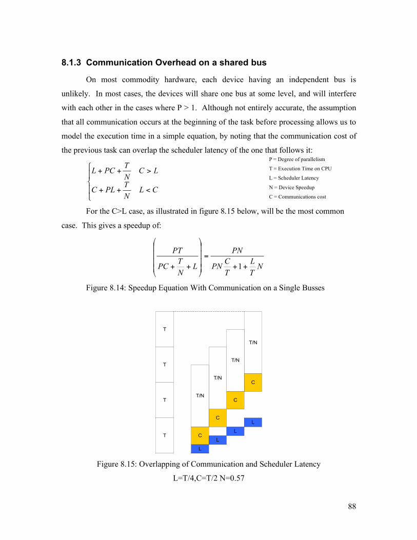
88
8.1.3 Communication Overhead on a shared bus
On most commodity hardware, each device having an independent bus is
unlikely. In most cases, the devices will share one bus at some level, and will interfere
with each other in the cases where P > 1. Although not entirely accurate, the assumption
that all communication occurs at the beginning of the task before processing allows us to
model the execution time in a simple equation, by noting that the communication cost of
the previous task can overlap the scheduler latency of the one that follows it:
!"
!#
$
<++
>++
CLN
TPLC
LCN
TPCL
For the C>L case, as illustrated in figure 8.15 below, will be the most common
case. This gives a speedup of:
NT
L
T
CPN
PN
LN
TPC
PT
++
=
!!!!
"
#
$$$$
%
&
++ 1
Figure 8.14: Speedup Equation With Communication on a Single Busses
L
L
L
L
T/N
T
T
T
T
C
C
C
C
T/N
T/N
T/N
Figure 8.15: Overlapping of Communication and Scheduler Latency
L=T/4,C=T/2 N=0.57
P = Degree of parallelism
T = Execution Time on CPU
L = Scheduler Latency
N = Device Speedup
C = Communications cost

89
Charts 8.20 through 8.25 show the speedup to break even in this case.
Comparison with the figures for independent busses show that for communication costs
less than 0.5T, they are nearly identical, but past that point, the shared bus
implementation will rapidly fall behind and become infeasible.
Of note is the fact that with a shared bus, communication costs equal to or greater
than the single processor time of execution cannot be tolerated regardless of P. On slow
busses, this will preclude jobs of even low complexity. For low speed busses, this can
limit the tasks used to those with high execution time per byte of data. When this is
combined with the fact that most devices will have a maximum job size they can
accommodate, it becomes apparent that only very complex jobs are feasible.
Charts 8.16 through 8.19, shown below, demonstrate how much communication
overhead cuts effective speedup in a shared bus setup.
Chart 8.16: Overall Speedup C=0.1T, N=2
Chart 8.17: Overall Speedup C=0.2T, N=2
Chart 8.18: Overall Speedup C=0.1T, N=4
Chart 8.19: Overall Speedup C=0.2T, N=4

90
Chart 8.20: Speedup Required To Break Event C = 0.1T On a Shared Bus
Chart 8.21: Speedup Required To Break Event C = 0.25T On a Shared Bus
Chart 8.22: Speedup Required To Break Event C = 0.5T On a Shared Bus
Chart 8.23: Speedup Required To Break Event C = 0.75T On a Shared Bus
Chart 8.24: Speedup Required To Break
Event C = 0.9T On a Shared Bus
Chart 8.25: Speedup Required To Break Event C = 0.975T On a Shared Bus

91
8.2 Testing environment
8.2.1 Overview
The analysis performed was done using simulation drivers that simulate actual
devices of varying complexity. As the goal of this analysis is to analyze the effectiveness
of the mapping and scheduling heuristics that are provided by this work, the lack of
actual hardware is acceptable. Even with this limitation, this environment will still allow
critical characteristics such a scheduler latency to be determined.
8.2.2 Device Simulation Driver
The device simulation driver used to test the system can model one or more
devices. The setup of these devices is determined adjusting constant data structures
before the device is compiled and loaded into the driver. This example driver can
supports all the interface functions defined for a driver, and models executions and
reconfiguration delays.
In addition to aiding the testing of the system, the simulation driver acts as a
template for the creation of real drivers, as it utilizes all of the interfaces needed to create
a real driver. The code is included in the appendix.
8.2.2.1 Simulated Execution
To keep the simulation simple, each device can support up to eight types of
operations. Each type of operation has a different set of coefficients that are used to
calculate how long a job will take to complete. These coefficients allow for the
estimation of how long the device will be processing (simulated by a delay where the
CPU is not used) and the cost of transferring information and setting up the device. It is
assumed that the host processor utilization happens up front before device execution.
The selection of which of the 8 cost calculations is made by the command
specified by the task. The first parameter of the task must be an integer immediate value,
and is used to calculate the job size. The host processor overhead is simulated by
transferring one byte of data from user space per unit of “cost” calculated. The time

92
when the device is working is simulated by the use of a timer, which wakes the calling
thread when the simulated device would have finished.
The cost calculations can be selected from a variety of common cost bounds listed
below in table Table 8.26: Simulation Driver Cost Approximation Functions. In this
table, N represents the job size, and a,b,c,d, etc. represent the coefficients. As floating
point math is not allowed in the kernel, all coefficients are treated as fixed point numbers
with a shift of 128, with the unit of jiffies or as a number of bytes.
Number Function
0 A
1 AN+BN2 + CN3 + DN4+C
2 A log2(N) ( approximate )
Table 8.26: Simulation Driver Cost Approximation Functions
8.2.2.2 Simulation of Configuration Latency
The loading of configuration code to a device is simulated in much the same way
as execution time. The exception is that the cost of loading the code is estimated using
only a single coefficient for latency and one for CPU utilization, based off the reported
size of the code being loaded. Asynchronous configuration is also modeled, but the
serialized CPU estimation is left out.
8.2.2.3 Limitations
The primary limitation of the simulation driver is the simplistic modeling of the
internal bus usage. This limitation means that is cannot be detected how devices may
interfere with each other under high bus utilization. As it is assumed that the
communication time of the tasks will be relatively small compared to the execution time
of the device, making collisions less important to model. This can be modeled by the
CPU time used at the beginning of each task, as it will exclude other tasks from running
by using CPU cycles, but that is an imperfect solution.
The other important limitation is that the timers provided in the kernel have a
resolution in jiffies. This is somewhere between 1ms and 10ms, preventing the modeling
of extremely small jobs.

93
8.3 Experiments Performed
Several different tests were performed to analyze the performance of the MHC
framework. These tests gauge the execution time when various features of MHC are
used, versus the serial execution time. These tests are done with a variety of settings in
order to demonstrate different strengths and weaknesses of the system. Each of the
subsections below describes one test run on the system.
These tests assumed that the user code uses MHC exclusively for execution of
tasks. Each test consists of submitting a known number of tasks to the MHC framework,
and timing the resulting execution. This was repeated under several different conditions,
as described below under each test. These conditions include varying task arrival rates,
hardware, dependency graphs, task completion time, and device suitability. The results
of these tests are presented in chapter 9.
8.3.1 Submission Time
The time required to submit a task adds directly to the overheads of the
framework, and limits the task grain size that can be reached. Because of the pre-
allocation behavior of MHC, the first time tasks are executed they will have significantly
higher submission times than later recurrences. As it is expected that most MHC enabled
applications will tend to use the same sets of tasks many times, the tests are repeated at
least twice, and the results from the second and later runs are used. The test times the
submission of the task separately from its execution by waiting for all tasks to reach the
appropriate queue, but not to complete.
The following parameters were varied for this test:
1. Features used – direct submission, online scheduler, dependency analyzer,
function library, and offline scheduler.
2. Number of tasks submitted concurrently
3. Number of devices

94
8.3.2 Total Execution Time
This test looks at the execution time of a set of tasks versus the time to execute
them serially. The total execution time metric is run using an application that generates
task graphs, with execution times that vary per device. Several different task graphs are
used to demonstrate how available parallelism affects the overall execution time, as well
as the effectiveness of different scheduling heuristics at taking the dependency
information into account.
The elements varied in this test where:
1. Variance of task execution times
2. Average task execution time
3. Variance in device suitability
4. Dependency graph used.
5. Dependency Graph width and height
When the task execution times or device suitability are varied, each task in the
task graph is assigned base completion time and a suitability per device on a random
basis. These numbers, once chosen, are kept static through the multiple repetitions of the
execution of the task graph used in the test.
In each case, the execution time is compared to the serial execution time to
determine speedup.
8.3.2.1 Dependency Graphs
The dependency graphs below where used to demonstrate the execution time of
the system. Each graph can be modified with a width M, and a height, N. In general, the
amount of parallelism for each graph is proportional to M, as indicated in below. N, the
height of the graph, is determined by after how many cycles MHCJoin is called to check
the results. These tasks below are designed to be representative of the types of
parallelism found in common computations.

95
8.3.2.2 Independent
This task graph is the case when dependency analysis is disabled, or when a
application has no dependencies between tasks. Essentially, M x N tasks are submitted
nearly simultaneously, with no dependencies. This models highly parallel jobs, which do
not make use of the dependency analyzer. Applications that map well in this category
include:
• batch image processing
• Multiple Object Classification
• Other highly parallel, very simple tasks
Available Parallelism: MNPi=
M
N
Figure 8.27: Independent Task Graph

96
8.3.2.2.1 Threads
This is similar to a number of separate threads of execution. This task graph
consists of a number of M independent threads, of length N. Where each member of the
thread is dependent upon the one submitted before it. This is the most basic from of
parallelism offered by most computer systems. Applications that map to this dependency
graph are similar to those in the independent task graph, but can be more complicated.
Examples include:
• Monte-Carlo Simulations
• Neural Network training
MPi=
M
N
Figure 8.28: Threads Task Graph

97
8.3.2.2.2 Distribute/Reduce
In this dependency graph, the submissions are divided into even and odd cycles,
where even cycles have M parallel tasks, and odd cycles have a single task that depends
on the M previous tasks. This graph represents algorithms which have a high degree of
parallelism for part of the program, but must collect, collate, or otherwise work with the
results as a group. This pattern is so common, that most parallel execution environments,
such as MPI or PVM contain function calls to automate it [25]. This method is
commonly called scatter/gather, but a different name is used here to avoid confusion with
the scatter/gather memory access techniques used by some drivers. Some examples
applications include:
• Genetic algorithms, which must consolidate simulation results to choose
the survivors for the next round of simulation;
• Object classification and feedback in a vision oriented control system.
• Any iterative solver which performs a convergence check after each
iteration.
This graph stresses the load balancing capacity of the scheduler, and will see an
increase in execution time when the task completion time or device suitability is varied.
!"#
$
$=
oddi
eveniMPi
1
M
N
Figure 8.29: Distribute/Reduce Task Graph

98
8.3.2.3 Dual Distribute/Reduce
The Dual Distribute/Reduce uses two instances of the Distribute/Reduce DAG,
offset by one cycle, preserving the load balancing test, while giving a constant task level
parallelism. Each level has M-1 instances that depend on one instance of the previous
cycle, and one instance that depend on M-1 instances in the previous cycle.
This DAG tests the load balancing, similarly to the one before, but will also test
the ability of the offline scheduler to increase the priority of tasks with more dependent
jobs. Although it would be unusual to find a real life application following this pattern, it
makes a good synthetic benchmark, because it tests the ability of the schedulers to
prioritize based on knowledge of the task graph.
MPi=
M
N
Figure 8.30: Dual Distribute/Reduce Task Graph

99
8.3.2.4 Fork/Join (divide and conquer)
This task graph is based on the behavior of an application that has an increase in
the amount of parallelism as it progresses, then has to reduce the results. This has a set
relationship between M and N, with N begin 2(log2(M)) + 1.
This pattern also tests the ability of MHC to determine the importance of a job
based on the tasks that depend on it. This task graph is unlikely to be generated by a user
who is not aware of the bulk of MHC features, but to an advanced user this graph could
give good performance for a variety of problems. This pattern is fairly common in many
different types of computation, such as the parallel sorting [25]. Although these
algorithms sometimes produce unbalanced graphs, this graph should still serve as a valid
benchmark.
!
Pi=
2i
i < N /2
2N" i"1
i # N /2
$ % &
M
N
Figure 8.31: Fork/Join Task Graph

100
8.3.3 Reconfiguration Hiding
This test looks at the handling of reconfiguration latency. It looks at the
following cases:
• All devices (except the CPU) have reconfiguration latency
• One device is reconfigurable, 4 are not
• One reconfigurable and one normal device.
Each of these scenarios was tested with the with a varying number of configurations
and device speedup. Also, the effect of varying configuration overhead relative to
computation time was investigated.
In order to allow the batch schedulers more time to collect data, the modeled user
behavior is assumed to perform tasks cyclically, with similar task sizes and patterns of
configurations recurring at regular intervals. This will be the case for many long running
jobs that use MHC, but may not be representative of short-term jobs. This is not an
impediment, however, as short term jobs probably cannot abide by the delay necessary to
configure a reconfigurable device.

101
Chapter 9: 9 Results
9.1 Submission Time
The results of the tests described in section 8.3.1 are shown below in the following
subsections. Each section also includes a discussions of the results, if necessary. For
each test, the result is the average over 50 trials. For comparison, the time to execute a
dot product of single precision 2000 element vectors on the test machine is 1.6 µs if it is
in cache and 7 µs if it is not cached.
9.1.1 Basic Submission
This test measured the time for a basic submission from user code to MHC,
including the time to allocate and initialize the task memory structures. The device
selected for each task was determined statically, so no scheduling heuristic or
dependency analysis overhead is included. When these results are placed into the
equations in section 8, it can be seen that with this implementation of MHC, most tasks
below 20us in execution time should not be considered. Although some tasks seen in
Chart 9.2 show a submission time as low at 5 µs, it is also not unusual for them to take as
high as 20us.
0
2
4
6
8
10
12
10 20 30 40 50 60 70 80 90 100 110 120 130 140 150 160 170 180 190 200
Task Subitted Simultaneously
mic
ros
ec
on
ds
Chart 9.1: Basic Task Submission
The average in chart 9.1 is more accurate than the histogram shown in chart 9.2,
because it uses a large number of trials between each time measurement. Tests showed
the time measurement system call itself introduces between 0 and 25 µs of error, with
about even distribution over that range. This makes it likely that the histogram should be

102
shifted somewhat towards higher latency. The average still indicates a completion time
of at least 20us for a task to be considered for a use with MHC.
Given that the submission latency is approximately equal to the data transmission
latency on the latest high performance networks [10,11], MHC should easily be able to
beat traditional networks on grain size if the latest internal interconnects are used.
0%
2%
4%
6%
8%
10%
12%
14%
16%
0~1
1~2
2~3
3~4
4~5
5~6
5~7
7~8
8~9
9~10
10~11
11~12
12~13
13~14
14~15
15~16
16~17
17~18
18~19
19~20
20~21
21~22
Time Range (us)
Perc
en
t o
f T
asks
Chart 9.2: Basic Task Submission Histogram

103
9.1.2 Task Submission Time with Online Scheduler
As shown below in chart 9.3, the latency of task submission rises with an increase in
the number of devices the online scheduler must consider. With a very large number of
devices, the submission time becomes less predictable as cache misses and other factors
come into play. Although it is unlikely that a single computer will have so many devices
supporting every job, the test was run with from 5 to 50 devices.
Chart 9.3:Task Submission Time With Online Scheduler.
As can be seen from this graph, the time to schedule a task depends heavily on the
number of devices that need to be considered. With 50 devices, the amount of
memory used to schedule each task comes close to 2 kilobytes, so when the number
of jobs is large, it begins to flirt with the limits of level 1 data cache on the test
machine.

104
9.1.2.1 Function Library Task Selection
This test measured the delay imposed when a function library is used to
automatically configure the task structure, calculate the ETC’s and select the
configuration for each device. As the automatic setup utilizes a fairly large set of data
repeatedly, it benefits from cache, as shown by the decrease in the average time as the
number of tasks increases, as shown in chart 9.4. When 50 devices where considered, the
amount of memory used to perform the automatic configuration exceeded the available
cache, as performance dropped off markedly, to the point where it could not be shown on
the same graph. This indicates that for a large number of devices to be used, more work
is needed to optimize the memory usage of the automatic task selection.
Chart 9.4:Submission Time with Automatic Setup
The results shown in 9.4 include the online scheduler and all other submission
times. It is apparent from this chart that the more of the decision-making is left to MHC
at run time, the larger the grain size useable will be. This suggests that the decision to
make the automatic components of MHC optional was not without merit. The oddity
here is the spike in the 5 device data series. This is not a transient happenstance, as it
appears in the average even over 50 trials. Due to its dependency on the threading
libraries the interface between the user-space and kernel-space parts of MHC are subject
to race conditions with the Linux thread scheduler. These races do not affect the
functionality, but they do effect the timing by delaying the submission of a few tasks
when a task submission occurs close to another process switch in the system. It was not

105
unexpected for certain test setups to have a higher propensity to encounter this condition
than others.
9.1.3 Dependency Analyzer
This tests the worst case situation for the dependency analyzer described in
section 5. Each task is submitted with one, five, or ten memory regions, in ascending
order. This will defeat the binary tree and give worst case timing. Chart 9.5 Depicts the
time taken to submit a job when the overlap-capable dependency analyzer is active.
Chart 9.6 depicts the same situation with the dependency analyzer in non-overlap
detecting mode.
Obviously, in the worst case the overlap handling dependency analyzer is order N,
resulting in the poor performance seen below when a large number of memory regions
are present in the system. This performance could be improved if a mechanism is put in
place to correct the unbalanced tree if it becomes too severe. As predicted, the non-
overlap handling dependency analyzer performs much better under the same
circumstances.
0
20
40
60
80
100
120
140
160
180
10 20 30 40 50 60 70 80 90 100 110 120 130 140 150 160 170 180 190 200
Jobs Submitted Simultanesously
mic
ros
ec
on
ds
1 Region/Task
5 Regions/Task
10 Regions/Task
Chart 9.5:Dependency Analyzer With Overlap

106
0
5
10
15
20
25
10 20 30 40 50 60 70 80 90 100 110 120 130 140 150 160 170 180 190 200
Jobs Submitted Simultanesously
mic
roseco
nd
s
1 Region/Task
5 Regions/Task
10 Regions/Task
Chart 9.6:Dependency Analyzer Without Overlap Detection
9.1.4 Discussion
Most of the cost of scheduling seen above, with the exception of the dependency
checker, is due to the decision to use threads instead of memory locking. Even though
this decision makes the system much more general, it was not without costs. The threads
themselves have an overhead of about 0.9us [21] per switch, given that the benchmark
above involved 2 context switches at a minimum, the cost is at least 18% of the
scheduling time. Also, the synchronization provided by the pthread library does not have
zero cost, and adds to the scheduling time as well.
The primary concern, however, is the uncertainty that comes from user level threads.
If the heuristic of submission time where extended, there would be a fraction of a
percentage that have submission times of several milliseconds. These tasks happen to be
interrupted after being requested, but before entering the kernel. Although rare, this
occurrence increases the average by 3 or 4 microseconds.
More up to date versions of Linux such as version 2.6 have pthread libraries with
lower latencies, which may help the latencies seen here fall to even lower levels.

107
9.2 Basic Scheduling Results
Unlike the results in section 9.1, the results of the experiments described in
section 8.3.2 do not provide information about the fundamental limitations of the MHC
framework presented here, but they do give an idea of what is possible with even modest
hardware resources under MHC and provides a chance to consider the effectiveness of
the example scheduling routines provided. The limitations stated in Chapter 8 should be
kept in mind when considering the results of the experiment.
9.2.1 Speedup overview.
These results give an overview of the speedup that occurs under a general case for
the different scheduling algorithms. For this experiment, both the job size and the task
suitability where varied. The speedup of the virtual devices connected to the system was
set to an average of 1, and the suitability for each job was set to be evenly distributed
between 0.5 and 2 (half as fast to twice as fast). The task size was set to vary by +-16%.
In order to allow room for this variation, the nominal task size was set at 15 time units, or
75ms. This task size essentially masks the costs exposed in section 9.1. As stated
above, this assumes independent busses, with the cost of communication factored in as
part of the suitability. Each of the graphs presented is an average over 10 runs.
By varying both the job size and the suitability, this tests both the load balancing and
device selection capabilities of the scheduling mechanisms. In each case, a line in the
graph called “base” has been included to help gauge the effectiveness of the device
selection. This line indicates synthetic perfect load balancing with no device selection or
suitability taken into account.
Each of the subsections below gives a graph and a brief description of the results.
For a discussion of the ramifications of these results, see section 9.2.3.

108
9.2.1.1 Independent Tasks
As shown below, when faced with a independent tasks, most of the schedulers
performed well with a low level of parallelism, selecting devices that provided the best
speedup for the jobs. At higher degrees of parallelism, the fast greedy online scheduler
and Best 2 batch scheduler failed to provide effective load balancing. Best 3 managed to
improve upon the real-time min min slightly by reducing the occurrence of a task
selecting a processor for load balancing reasons and denying a task submitted later access
to the device it is most suited for.
0
1
2
3
4
5
6
7
8
9
1 2 3 4 5 6 7 8 9 10 11 12 13 14 15 16 17 18 19 20
Degree of Parallelism
Sp
ee
du
p
Fast Greedy
Min-Min
Best 3+min min
Best 2+min min
Base
Chart 9.7:Independent Tasks

109
9.2.1.2 “Threads” DAG
0
1
2
3
4
5
6
7
8
9
1 2 3 4 5 6 7 8 9 10
DAG Width
Sp
eed
up
Fast Greedy
Min-Min
DAG+geedy
DAG+min min
Best 3+min min
Best 2+min min
Base
Chart 9.8:”Threads” Graph, Depth = 4
The threads graph limits the number of tasks available at any given time due to
the dependencies between the tasks. This has the benefit of delaying the submission of
some tasks, and improving the load balancing, as shown by the improved performance
relative to the “base” line. Again the Best 3 scheduler in combination with the real-time
min min scheduler was the most effective.

110
9.2.1.3 Distribute/Reduce task graph.
0
1
2
3
4
5
6
1 2 3 4 5 6 7 8 9 10
DAG Width
Sp
eed
up
Fast Greedy
Min-Min
DAG+geedy
DAG+min min
Best 3+min min
Best 2+min min
Base
Chart 9.9:”Distribute Reduce” Graph, Depth = 4
This graph really shows the benefit of heterogeneity over a traditional
multiprocessor. On a traditional multi-processor box, the limit of the degree of
parallelism on the odd stages of the graph would reduce the maximum speedup. Because
in most cases at least one of the devices has a speedup greater than one for this task,
MHC allows for a higher overall speedup than a perfect balance across homogenous
devices.

111
9.2.1.4 Dual Distribute/Reduce task graph
0
1
2
3
4
5
6
7
2 3 4 5 6 7 8 9 10
DAG Width
Sp
eed
up
Fast Greedy Min-Min
DAG+geedy DAG+min min
Best 3+min min Best 2+min min
Base
Chart 9.10:”Dual Distribute Reduce” Graph, Depth = 4
This task graph really stresses the load balancing and task selection. The large
number of available tasks with varying suitability at any point in time makes scheduling
online more difficult, but also more important. The performance of the online schedulers
here is hindered by the “gateway” tasks (those at the narrow part of the DAG) competing
for the most suitable devices with the tasks from the second graph. The DAG provides
some help in prioritizing the large number of tasks when the width is high, but hinders
performance when the number of devices is plentiful compared the number of tasks that
are ready to execute.

112
9.2.1.5 Divide and Conquer task graph.
0
1
2
3
4
5
6
7
8
9
10
1 3 5 7 9 11 13
DAG Height
Sp
eed
up
Fast Greedy
Min-Min
DAG+geedy
DAG+min min
Best 3+min min
Best 2+min min
Chart 9.11: Divide and Conquer Task Graph
This task graph seems to differentiate between the different scheduling algorithms
nicely at low heights. When the task graph becomes very large, the performance of the
scheduling algorithms that attempt to load balance falls off quite sharply. The cause is
not immediately obvious from the graph, but becomes clearer when the number of
available tasks at each depth is considered.
At a depth of 13, the middle layer is composed of 64 tasks. These are scheduled
in the order they are requested by the test program, which is left to right. This results in
the tasks on the left hand side finishing much sooner than the tasks on the right, which
due to the load balancing can be shortsightedly placed on non-optimal devices. The tasks
further to the right that are better suited to that device are then prevented from using it in
a timely manner. When the results are “reduced” to get the final result, tasks have one of
their dependencies resolved much later than the other, reducing the available parallelism
at those times and rendering the load balancing less effective.
This behavior can be best illustrated by the fact that at a height of 13 nodes, the
best 2 outperforms the best 3, indicating its stricter policy of which devices to consider
for scheduling reduced the negative effect of load balancing in this case. The fact that
best 3 is also outperformed by basic min-min (equivalent to best 5) indicates that in
addition to limiting the number of devices considered to avoid the creation of these

113
circumstances, having more alternatives for the tasks that fail to find their optimal
machine can also reduce the impact of this effect.
9.2.2 Testing the DAG batch scheduling algorithm
In the tests above, the addition of the algorithm based on [4] failed to provide
meaningful speedup over the online scheduler algorithm it is paired with. This test sets
out to create a circumstance where the problems corrected by this batch scheduler will be
more common. The dual distribute/reduce graph test above was modified such that the
points where the graphs are restricted could only run on a single device. Also, the task
suitability was set to vary between a speedup of 0 and 1. This creates a situation where
the tasks at the constricted points should get higher priority.
As shown in the graph below, the despite the poor showing of the DAG scheduler
above, it does have some value under certain circumstances. The frequency with which
those circumstances occur in actual applications mapped to MHC remains to be seen,
however.
0
0.5
1
1.5
2
2.5
3
3.5
4
4.5
1 2 3 4 5 6 7 8 9 10
Task Graph Width
sp
ee
du
p
RT min min
DAG + RT min min
Chart 9.12: DAG Advantage

114
9.2.3 Heuristic test result ramifications
The results in the previous sections all illustrate the importance of having a
flexible system for allowing the user to choose the heuristic that is correct for their
application. The tests above showed that in most situations, the online scheduler
functioned admirably. It has sufficient margin for manipulation to allow for the
implementation of online scheduling routines such as min-min. These tests show that the
single measurement heuristic of fast greedy, while valid when the available resources
exceed the available parallelism available in the application, the more complicated online
schedulers can do better in situations where many jobs are available for scheduling
concurrently.
The simple batch scheduler best 3 combined with the min-min online heuristic
showed a small improvement over the online heuristic alone. However, in most of the
generic tests the DAG based batch scheduler failed to perform better than the online
scheduler alone, and in some cases the cost of running the algorithm was high enough
that it performed slightly worse.
The initial algorithm in [4] upon which the DAG scheduler was based used the
statically calculated time distance to the node that provides the final result to calculate the
priority. Because MHC cannot know which node is the terminal node of the DAG, and
may have more than one terminal node, the effectiveness of this scheduler is reduced.
These results show that in most cases, the effectiveness was reduced by this shortcoming
much more than was expected. However, chart 9.12 indicates that in some cases, this
heuristic can give a ~30% improvement in speedup over the online scheduler alone.
Overall, these results indicate that creating MHC with a “one-size fits all”
approach in schedulers would undermine its usefulness, and validate the design
philosophy of a flexible, modular system. Furthermore, these results show that the
implementation created by this work can provide the functionality desired from MHC.

115
9.3 Reconfiguration Latency Handling
This section contains graphs and charts illustrating the effectiveness of the various
reconfiguration-handling mechanisms proposed in the system. The data presented is
chosen not for covering a large number of possible setups, but to indicate particular
points of interest. The following graphs depict the speedups of the system as a whole
then there is one CPU, and 5 reconfigurable devices, each of which has a speedup of 2
compared to the processor.
9.3.1 5 Reconfigurable devices
The case where the reconfiguration latency is not handled at all was not
considered for this setup, as it is obviously unsuitable. The graphs in order show the
effects of reconfiguration equal to one half, one, ten, and 100 times the execution cost on
the reconfigurable device.
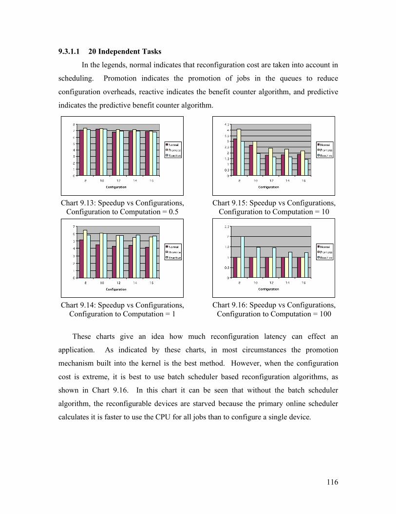
116
9.3.1.1 20 Independent Tasks
In the legends, normal indicates that reconfiguration cost are taken into account in
scheduling. Promotion indicates the promotion of jobs in the queues to reduce
configuration overheads, reactive indicates the benefit counter algorithm, and predictive
indicates the predictive benefit counter algorithm.
Chart 9.13: Speedup vs Configurations,
Configuration to Computation = 0.5
Chart 9.14: Speedup vs Configurations,
Configuration to Computation = 1
Chart 9.15: Speedup vs Configurations,
Configuration to Computation = 10
Chart 9.16: Speedup vs Configurations,
Configuration to Computation = 100
These charts give an idea how much reconfiguration latency can effect an
application. As indicated by these charts, in most circumstances the promotion
mechanism built into the kernel is the best method. However, when the configuration
cost is extreme, it is best to use batch scheduler based reconfiguration algorithms, as
shown in Chart 9.16. In this chart it can be seen that without the batch scheduler
algorithm, the reconfigurable devices are starved because the primary online scheduler
calculates it is faster to use the CPU for all jobs than to configure a single device.

117
9.3.1.2 Two Threads, Five Configurable Devices
This test used two threads, with a task graph depth of either 10 or 20. For these tests,
the devices where started with random configurations. This effects only the results of
Chart 9.16, as it allows the promotion method to utilize the reconfigurable devices when
a task happens to use one of the configurations.
Chart 9.17: Speedup vs Configurations, Configuration to Computation = 1
Chart 9.18: Speedup vs Configurations, Configuration to Computation = 10
Chart 9.19: Speedup vs Configurations, Configuration to Computation = 100
These results do not favor the predictive scheduler; in chart 9.19, it demonstrates
how poorly it performs when there is insufficient depth to the task graph for it to pre-
schedule configuration changes with any accuracy. In that case, the time spent changing
configurations inappropriately results in a speedup less than one.
Other points of note are that in most cases, the reactive benefit counter scheduler out
performs all others, which contrasts with the results in the section above where the high
number of concurrent tasks gave the promotion method the advantage.
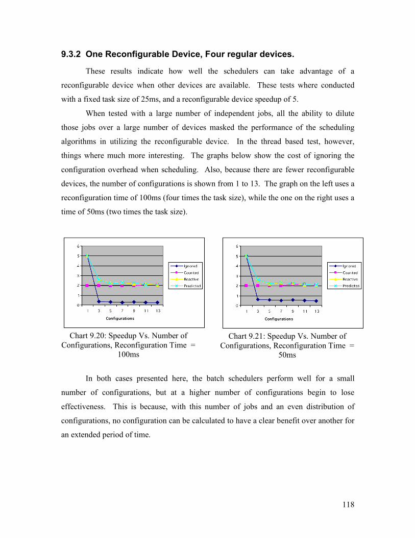
118
9.3.2 One Reconfigurable Device, Four regular devices.
These results indicate how well the schedulers can take advantage of a
reconfigurable device when other devices are available. These tests where conducted
with a fixed task size of 25ms, and a reconfigurable device speedup of 5.
When tested with a large number of independent jobs, all the ability to dilute
those jobs over a large number of devices masked the performance of the scheduling
algorithms in utilizing the reconfigurable device. In the thread based test, however,
things where much more interesting. The graphs below show the cost of ignoring the
configuration overhead when scheduling. Also, because there are fewer reconfigurable
devices, the number of configurations is shown from 1 to 13. The graph on the left uses a
reconfiguration time of 100ms (four times the task size), while the one on the right uses a
time of 50ms (two times the task size).
Chart 9.20: Speedup Vs. Number of Configurations, Reconfiguration Time =
100ms
Chart 9.21: Speedup Vs. Number of Configurations, Reconfiguration Time =
50ms
In both cases presented here, the batch schedulers perform well for a small
number of configurations, but at a higher number of configurations begin to lose
effectiveness. This is because, with this number of jobs and an even distribution of
configurations, no configuration can be calculated to have a clear benefit over another for
an extended period of time.
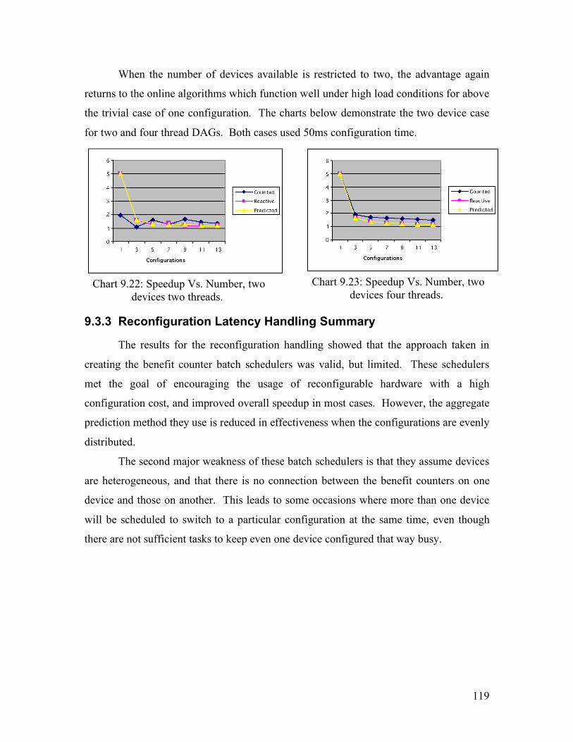
119
When the number of devices available is restricted to two, the advantage again
returns to the online algorithms which function well under high load conditions for above
the trivial case of one configuration. The charts below demonstrate the two device case
for two and four thread DAGs. Both cases used 50ms configuration time.
Chart 9.22: Speedup Vs. Number, two devices two threads.
Chart 9.23: Speedup Vs. Number, two devices four threads.
9.3.3 Reconfiguration Latency Handling Summary
The results for the reconfiguration handling showed that the approach taken in
creating the benefit counter batch schedulers was valid, but limited. These schedulers
met the goal of encouraging the usage of reconfigurable hardware with a high
configuration cost, and improved overall speedup in most cases. However, the aggregate
prediction method they use is reduced in effectiveness when the configurations are evenly
distributed.
The second major weakness of these batch schedulers is that they assume devices
are heterogeneous, and that there is no connection between the benefit counters on one
device and those on another. This leads to some occasions where more than one device
will be scheduled to switch to a particular configuration at the same time, even though
there are not sufficient tasks to keep even one device configured that way busy.

120
Chapter 10 10 Future Work
10.1 Overview
This section details the many possible improvements to the framework presented in
this work. In each of the following subsections, various ideas are introduced and briefly
discussed as to the effect they would have on the system if implemented. Some of these
recommendations for expansion have suggestions of possible implementations or ways of
interfacing to the existing system.
10.2 Caching and Coherency
Currently, the MHC framework presented herein relies on all data being written
back to the primary memory between tasks, and then loaded by any devices that need it.
As the analysis in section 8.1.3 shows, the cost of this communication can greatly limit
the speedup achieved, even on very fast hardware. Most high performance CPU's avoid
this overhead by utilizing cache on board the CPU to remember recently used data.
Exploiting data locality is a well known concept in both general and heterogeneous
computing, and some scheduling algorithms give priority to machines who ran tasks that
provide the dependencies of the task being scheduled [8].
As MHC does not specify any particular bus architecture or connection scheme
for physical hardware, the number and types of caching could vary greatly. It is possible
for a device to be similar to a cpu and have hardware coherency maintained memory, it is
also possible for a device to have a large amount of local memory, in a completely
separate space from the primary memory store.
In the first case, no modification would be necessary for MHC to take advantage
of the cache, and a batch scheduler could be created to increase its effectives using an
algorithm such as Weighted RT min min. [8].
The far more likely case is that most of the devices will have independent
memory spaces, and will happen to retain copies of the data they where sent to work on.
Thanks to the dependency analysis that can be enabled, full coherency does not need to

121
be maintained. Only when a job is starting or the user is about to access memory is it
important to make sure that the memory is coherent.
One possible implementation is a fast lookup hash table capable of tracking
device caching and ownership of memory regions. This lookup system would be
responsible for tracking who has local copies of which data, and who has dirty copies of
the data. Any task that writes to a memory region can be assumed to mark that region as
dirty, and to invalidate the memory region for all devices that are reading from it. Also,
any call to MHCJoin() for a memory region should result in all devices making any
overlapping caches they have coherent with memory before the call returns. Devices
should not even keep the data buffered unless they have hardware supported coherency,
as the user may write or read any memory in the region after they call MHCJoin.
In order to support this, several additions would need to be made to the interfaces
within MHC. Firstly, an addition to the notify function would allow for devices to
indicate to the kernel module which code they are caching, and whether it is dirty
(inconsistent with main memory) or clean. Also, any driver that supports caching will
need a function to flush the cached data and invalidate it. This invalidation functionality
must be exposed to user space as well so that the MHCJoin and dependency analyzer can
be appropriately updated.
Early versions of the parameterization method used for the passing of data called
for a bit to enable or disable caching. This was later decided to be unnecessary for the
functionality being implemented, but sufficient bits remain unused in the type field that
such a bit could be added, although a recompile of the affected drivers would most likely
be required.
10.3 Automatic Task Aggregation
One possible way to improve performance using the dependency graph is to
automatically aggregate tasks into larger tasks, and dispatch them as a group to a single
device. Although in general MHC aims to use as small a grain size as possible, if
sufficient parallelism can still be achieved to utilize the available hardware, it could be
beneficial to group related tasks of a similar type and place them on a single device to

122
minimize communication overheads. It is also possible that such aggregated tasks could
be large enough to be sent to other hosts over a network for processing.
This mechanism of improving performance will mainly overlap with the caching
described above, and would require more complicated analysis of the DAG in order to
accomplish.
In order for this to be effective, a group of tasks in a DAG should depend upon
each other, and have a available degree of parallelism low enough not to starve other
devices if they are grouped. Also, the benefit will be lost if any of these tasks (other than
the first one) depend on tasks outside of the group, as the combined metatask could not
be dispatched until all such dependencies are resolved.
10.4 ETC Prediction/Automatic Profiling
This work assumes accurate ETC prediction parameters are available for the
execution of tasks on the CPU, but does not specify how this prediction information is
generated or obtained. Although a static method where the timing estimates come with
the library may work passably well, it is true that all general purpose processors do not
share the same suitability for all different algorithms.
An automatic system that generates the correct parameters would be useful to the
system. A test that performs several trial runs per piece of code to generate the execution
estimation constants would be effective, but could take an inordinate amount of time.
The integration of a profiling mechanism for both code and hardware would allow for
new libraries to be introduced to the system quickly by generating the constants by
comparing the hardware and software profiles.
10.5 Memory Locking Option for Jobs with Small Memory
Regions
As discussed in section 4.6, the locking of memory or kernel space buffering of
memory requested by tasks is avoided for a number of reasons, the most series of which
is the fact that the memory locking of large regions of memory while the task is just
sitting in the queue could result in thrashing. As a result of this decision, a task has to
123
undergo four or more context switches after it is submitted to the kernel in order to make
sure its memory is available. Although the cost of a context switch is small, it still makes
up a meaningful part of the scheduling cost, which as shown in chapter 8 is critical to the
grain size achievable by MHC.
As jobs with a small task size are the least likely to cause a problem if they use
memory locking, and are the most likely to suffer the negative effects of higher
scheduling time, it would make sense to enable memory locking for those jobs. This
would mean that a thread submitting a task does not need to be awoken when its task
reaches the head of the queue, just when it is completed, reducing the overall scheduling
time and CPU utilization.
Linux already has a number of kernel level functions that automate the process of
locking a memory region for IO and mapping it to kernel space, which simplifies a
potential implementation. All that would be needed was a new function in the scheduler
that detects when a job has small enough memory regions that they can all be locked, that
it is scheduled on a device that supports this behavior. If the kernel module succeeds in
locking the memory it will map all the memory regions (parameter list, device
configuration, etc.) into kernel space. A new function would be added to the interface
with a device, which allows a submission from kernel space without the associated thread
being woken up. Also needed is an addition to the MHCNotify function to allow the
driver to indicate to the kernel module that the task has been completed, and a method of
asynchronously notifying the base library of task completion.
Looking at the results of a benchmark for context switch time [21], this could
save approximately 2µs off the cost of submitting a task. If this functionality is exposed
to user space (which would require additional flags in the submit call, and a new method
of notifying the dependency analyzer of task completion), the need for additional threads
and the synchronization overhead they entail could be eliminated for small tasks, possibly
reducing submission time by 4 or more microseconds off the 10 µs listed in chapter 9 for
tasks that are small enough to be locked. Other benefits include more consistency in job
submission times, as the number of simultaneous competing threads will be reduced.
As the job size which can be safely submitted this way will vary with the
resources of the system, a user configurable setting at the system wide level for the size at

124
which a task will make use of locked memory would make sense. With the proliferation
of 64 bit machines and cheap memory, this access method may, in the future be used by
all but the largest of tasks.
10.6 Impact of Dynamic Queues on MHC
The primary limitation on which schedulers can be implemented in this work is
the idea that the queues are FIFOs. Although in the minority, some schedulers, such as
that in [20], use priority queues, and even allow the priority to change after a job has been
inserted. In this work, such queues where avoided in order to prevent starvation or other
phenomena that can occur with non FIFO queues in a multi-user system. The only
exception being for the reconfiguration latency hider when promotion is enabled, which
even then is limited to prevent starvation.
It is likely that there will be many systems that do not need to guarantee fairness
between multiple users, and which would benefit from the more exotic queuing
algorithms, so it should be feasible to enable dynamic queuing as a administrator enable
option.
In order to implement this, the changes that need to be made are small. A new
queuing algorithm would need to be written in the kernel, and an interface would need to
be added for the dynamic alteration of job priority. Also, one or more batch schedulers to
take advantage of the new functionality would be needed.
10.7 Back Annotation of ETC Predictions to Improve Accuracy
It is unlikely that even the most sophisticated prediction system will be accurate
all the time in predicating the ETC of tasks. In fact, due to the lack of any simple way to
measure or predict internal bus utilization, it is likely that the ETCs predicted will only
serve as rough estimates. One possible solution is to set up a feedback path to the ETC
prediction logic that would allow it to take into account the errors in its previous
predictions when calculating the estimated completion time for a new task.
Such a system would be simple to implement on the kernel side, all that would be
required would be an additional field in the task structure, which would be filled with the
actual completion time when the task completes. On the ETC prediction side, things do

125
not have to be much more complicated. As most applications will tend to repeat similar
combinations of task requests, simply remembering the percent error per device would
make ETC generation more accurate. As the utilization of busses and other resources
will also tend to vary cyclically, a more complicated algorithm which takes into account
the position in the DAG or count of submissions since the last MHCJoin() could be
helpful, perhaps using similar logic to a global history based branch predictor to index the
correct estimation of error at a given time.
10.8 Integration of More Options for ETC Prediction
The work as presented uses a very naïve, polynomial based ETC prediction
system. As indicated in the introduction, while this work was being completed, a parallel
work [14], was concluded that proposed multi-cord as better prediction method. The
integration of the new prediction method should be strait forward, although it could break
compatibility with existing device and library descriptions if not handled properly. As
there are currently no third party libraries or devices, this should not be a problem is it is
done early enough.
10.9 Creation of MHC Compliant Hardware / Drivers / Libraries
As indicated in the introduction, this work provides the overall framework, and
some examples that would be useful in implementing an actual library or device driver.
Needless to say, if work is to continue on MHC, one of the projects that must be
undertaken in the future is to create an actual hardware driver and library for use with
MHC.
10.10 More/Better Batch Scheduling Heuristics
The Scheduling heuristics presented in this work, although effective, are only
examples of what is possible. MHC is designed to be very flexible, and allow for many
different implementation of scheduling heuristics. As research into scheduling heuristics
was not the primary goal of this work, there is plenty of room left for the development of
new schedulers to improve performance.

126
10.11 “Stackable” batch schedulers.
As batch schedulers are currently modular with respect to MHC, the user can easily
swap them in an out. Currently, the system only allows one batch scheduler to be in use
at one time. This prevents beneficial combinations, such as a combination of Kbest and
the reconfiguration hiding offline scheduler, from being implemented without writing and
entirely new scheduler.
There are no inherent limitations of the system that would prevent this, and it could
be realized with some simple modifications. The only additional data needed would be
needed is an additional system accessible field in the MHCOfflineScheduler data
structure to form a list and a global pointer. Two functions would then exist that advance
the global pointer and make the appropriate calls on the correct schedulers, and then
make the actual submission calls to the rest of the MHC framework when the list is
exhausted.

127
Chapter 11: 11 Conclusion
The framework produced in this work provides all the necessary components to
integrate hardware and begin real world testing of MHC. The automatic dependency
analysis and function library frameworks created in this work meet the primary goals of
user transparency and automatic mapping of tasks. The scheduling implementation is
extremely flexible, and allows for a large variety of scheduling algorithms to be explored,
encouraging future research in this area, as recommended in [8].
The results obtained by testing this framework with virtual devices validate the
feasibility of MHC. Based on the scheduling latency, MHC can target a grain size well
under 100µs for jobs with high complexity. The analysis shown indicates that the
utilization of fast internal communication fabrics is, as the proposal of MHC indicated,
the cornerstone of decreasing the grain size and increasing the effective parallelism of
user applications. The lack of actual hardware was not a hindrance to the measurement
of the internal latencies, as the actual hardware does not influence the scheduling delay.
The lack of actual hardware did limit the examination of speedup obtained to
larger grain sizes that the simulation drivers could handle. Even so, the simulation
drivers did allow for the framework to be verified and stress tested and debugged under a
variety of loads. It also allowed the comparison and testing of the scheduling methods
and reconfiguration handling methods implemented.
The reconfiguration latency handling methods introduced show some success at
increasing the utilization of high reconfiguration time devices, while minimizing the
impact of the reconfiguration. These algorithms are unique in that they dynamically
handle the scheduling of reconfiguration in an environment where the option exists to
utilize other hardware while waiting for the reconfiguration to complete. The results
obtained indicate that the while the reconfiguration handling methods are effective, there
is still research to be performed in this area.

128
The analysis performed in this work also explains the seemingly poor
performance seen in [8], even though the speedup of each device was an optimistic 20.
As shown in Section 8.1, the speedup of the overall system is very insensitive to speedup
of individual devices when communication time is high and the benefit of MHC will
remain almost exactly as high if the speedup is reduced. In fact, the benefit of MHC can
perhaps be best demonstrated with a speedup as low as 1.
In conclusion, this work should serve as a firm basis for future research into
Micro-Heterogeneous Computing. As noted in chapter 10, there is still much room to
experiment and improve MHC. Even so, the framework presented in this work is
complete and functioning, and with the additional of MHC compliant hardware and
libraries would become the first functioning Micro-Heterogeneous system.

129
12 References
[1] Compton, K, and Hauk, S. (1999). “Configurable Computing: A survey of systems and software” Northwestern University, Dept. of ECE, Technical Report .
[2] Freund, R. F. et al. (30 March 1998). “Resources in Multi-User, Heterogeneous, Computing Environments with SmartNet,” Seventh Heterogeneous Computing Workshop Proceedings, Page(s): 184 –199.
[3] Goran, M. et al. “Static-Dynamic Mapping in Heterogeneous Computing Environment,” International Symposium on Virtual Environments, Human-Computer Interfaces, and Measurement systems, Lugano Switzerland, 27-29 July 2003.
[4] Iverson, M. and Özgüner, F. (30 March 1998 ). “Dynamic, Competitive Scheduling of Multiple DAGS in a Distributed Heterogeneous Environment,” Seventh Heterogeneous Computing Workshop Proceeding, Page(s): 70 –78.
[5] Maheswaren, M. et al. (12 April 1999). “Dynamic Matching and Scheduling of class Independent Tasks onto Heterogeneous Computing Systems”, Eighth Heterogeneous Computing Workshop Proceedings, Page(s): 30 –44.
[6] Russel, R. P. ( 2000 ). “Unreliable Guide To Hacking The Linux Kernel” http://kernelbook.sourceforge.net/kernel-hacking.html/ ( May 6, 2003 ).
[7] Salzman, P. J, “The Linux Kernel Module Programming Guide,” ( ver 2.4.0 ) http://www.tldp.org/LDP/lkmpg (Accessed May 6, 2003 )
[8] Scheidel, W. L. “Efficient Utilization of Fine-Grained Parallelism using a micro Heterogeneous Environment.”
[9] Shabaan M. et al. “A User-Transparent Architecture for Micro-Heterogeneous Computing Systems,” Proposal to Thirteenth Heterogeneous Computing Workshop.
[10] “Introduction to InfinibandTM.” Mellanox Technologies. Rev 1.9. Available: http://www.mellanox.com/technology/shared/IB_Intro_WP_190.pdf
[11] “Latency Results from Pallas MPI Benchmarks.”(December 2, 2003). Virtual Machine Interface 2.0. Available: http://vmi.ncsa.uiuc.edu/performance/pmb_lt.php
[12] Hatchman, M. (Februrary 4, 2004 ). eWeek. Available: http://www.eweek.com/article2/0,4149,1515826,00.asp
[13] Fried, S. (April, 2003). “First Look: The AMD Opteron™ Processor.” HPCTimes. Available: http://www.microway.com/newsletter/newsletter-April2003.doc

130
[14] Goltsman, M. ( February 19, 2004 ). “Performance Estimation Techniques for Micro-Heterogeneous Computing.”
[15] http://www.rit.edu/~meseec/
[16] Maheshwari, P. (1996). “Dynamic Load Balancing Algorythms for a Heterogeneous Computing Environment.” Proceedings of the 29th Annual Hawaii International Conference on System Sciences.
[17] “Configureing FPGA’s”. StarBridge Systems: Tutorials. Available: http://www.starbridgesystems.com/concepts/15_FPGA_configuring_Medium.mov
[18] “Pci Protoboard: PCI Controller”. Available: http://www.techniprise.com/pci_protoboard.htm#PCI%20Controller
[19] Karthikeya, M. et al. “Partitioning in Time: A Paradigm for Reconfigurable Computing”
[20] Ghiasi, S. and Sarrafzadeh, M. (2003) “Optimal Reconfiguration Sequence Management”
[21] Molnar, I. (August 5, 2002 ). “Re: context switch vs. signal delivery.” Available: http://www.cs.helsinki.fi/linux/linux-kernel/2002-31/0272.html
[22] Culler, D. E. and Singh, J. P. ( 1999 ). Parallel Computer Architecture (PCA): A Hardware/Software Approach.
[23] “Computation on GPUs.” Siggraph 2003. http://www.csit.fsu.edu/~blanco/siggraph03/siggraph_2003.htm#GPU
[24] Kim, J. K., et. al. (2003). “Dynamic Mapping in a Heterogeneous Environment with Tasks Having Priorities and Multiple Deadlines” Proceedings of the International Parallel and Distributed Processing Symposium.
[25] Allen M., Wilkinson, B. (1999). Parallel Programming: Techniques and Applications Using Networked Workstations and Parallel Computers. New Jersey: Prentice Hall
Unless otherwise specified, conference articles available online through the IEEE at ieeexplore.ieee.org

131
Appendix A: Included Files, Compilation, and Installation
Make Files
Path Description Top Level Makefile source/makefile The makefile used to build the entire project.
Library Makefile source/base_lib/makefile makefile used to build the base library.
Kernel Module Makefile
source/kernel_mod/makefile makefile used to build MHC kernel module.
Test File Makefile source/test/makefile builds various test programs and the example MHC compliant simulation driver.
Kernel Module Source
Path: source/kernel_mod
File Description MHC.h Contains basic data structures and defines used by both the kernel module and
the user level libraries. MHCCode.h
Contains data structure definitions for the description of device code or configuration information passed from userspace.
MHCDevice.c Contains code for interfacing with devices and device drivers. MHCDevice.h
Contains the data structures used in storing the status of the devices and communicating with the device drivers.
MHCInterface.c Contains the interface to the userspace libraries, in the form of an ioctl handler. MHCioctl.h
Contains the definitions of the ioctl command numbers for each of the commands the kernel module recognizes.
MHCModule.c
Contains the initialization code to install the module into the kernel and initialize key data structures.
MHCParams.h
Contains the definition of the format used to specify memory regions as input or output from functions in MHC
MHCQueue.c Contains basic queue management routines. MHCQueue.h Contains queue data structures. MHCScheduler.c Contains the online scheduling code and statistics gathering information. MHCScheduler.h Contains prototypes for scheduler functions.

132
Kernel Module Source
Path: source/base_lib
File Description
Dependancies.c Dependency analysis and memory region tracking implementation Dependancies.h Dependency analysis and memory region tracking data structures dprintf.h Debugging output control MHC.c Startup and shutdown functions for MHC. MHCLibAssist.h Function library setup data structures and prototypes. MHCLibAutoSetup.c Automates function library setup and registration. MHCLibCache.c Caches device code and configurations. MHCLibCleanup.c Code to clean up function libraries when they are no longer needed. MHCLibParse.c Code to parse function library files. MHCList.h List management inlined code. MHCOfflineReconfig.c Offline scheduler designed to compensate for long reconfiguraiton times. MHCOfflineScheduler.c Example batch scheduler implementations. MHCOfflineScheduler.h Static data structures and prototypes for example batch schedulers. MHCSchedulers.c Code for controlling which scheduling mechanisms are chosen MHCSchedulers.h Interface description for scheduler control. MHCTask.c Contains code for controlling tasks. MHCTask.h Task data structure. MHCWrappers.c Wrapper functions for kernel access. MHCWrappers.h Wrapper functions for kernel access prototypes. SubmitThreads.c Thread control and submission code. SubmitThreads.h Prototypes and data structures used to manage the “worker threads” TaskControl.c User callable functions to manage tasks. TaskControl.h Prototypes of task management functions. TaskMonitor.c Code for initializing, linking, and disposing of task monitors. TaskMonitor.h Data structures used to store task state and display it to the user. TaskMonitorList.h A simple list of task monitors, used to queuing and set building.
Example Library Files
Path: examples/
File/Directory Path Description
function_libs Example directory structure of function libraries. MHC_GSL function_libs/MHC_GSL/ Function library description file, w/ comments. MHCDevices Example device directory.
Compilation
Compilation is very simple, in the source directory, type make. Some minor
modification may be necessary based on the compiler used. The code has been tested
with icc and with gcc. Between kernel versions 2.4 and 2.6, the method used for the

133
compilation of kernel modules changed dramatically, so in newer kernel versions the
makefile will need to be changed.
Installation
There is no installation script currently, so it is up to the user to decide where to
place the library files and executables created during the build. The installation
procedure is as follows:
1. Move include files and library files to appropriate locations
a. The compilation will create an include directory. The contents
should be moved to the directory of your choice, but
/usr/include/MHC is recommended
b. Both a shared and a static library will be created in the base_lib
directory.
2. Create the function library and MHCDevice paths.
a. The default MHC directory is set in file MHCLibAutoSetup.c.
b. Use the example directory structure described in the example
folder on the included CD.
3. Install the kernel module
a. This can be done with the script add_mgc.sh
b. This requires a kernel compiled with module support
c. This will not occur automatically at each boot unless added to the
startup scripts.
d. After the MHC module is installed, individual MHC compatible
device drivers can be added into the kernel.

134
Appendix B: Test Code and Utilities Utilities mhctop
source/test/mhctop.c
This file compiles to a program similar in function to top. It displays the
utilization of each installed device. If invoked with the –D option, it will provide detailed
information on each queue.
mhc_set_flags
source/test/mhc_set_flags.c
This file compiles to a program that allows the flags for each device to be set,
cleared, or viewed. When installed, the program is meant to be linked under the names
mhc_get_flags and mhc_clear_flags as well. Only root can change the flags.
The usage for the set and clear variants is:
mhc_<set|clear>_flags <device id> flags
For mhc_get_flags, it takes an optional device id. If the device id is not specified
it lists the flags for all devices. The flags are:
• E – allows exclusive access.
• S – enables starvation check
• P – enables the “promotion” reconfiguration optimization.

135
Test Software Test Driver
/source/test/testdriver.c
This file contains the source for a device driver with MHC support. It is designed
to test the various features of MHC. To keep it as simple as possible, to change the
configuration of the devices it simulates, the driver must be recompiled and re-inserted
into the kernel. It supports several different each job submitted to a device has its
execution time, configuration time, etc. generated from the parameters passed to the job.
A number of different equations are supported to determining these values, and can be
configured by an array towards the top of the file. Any number of devices up to the
maximum number supported by MHC can be simulated, but due to the lack of any
modeling of bus contention, the accuracy of the simulation would decrease if a very large
number of transfers are simulated concurrently.
Performance Test Generating Program
/source/test/
This program allows the testing of MHC with a variety of Directed Acyclic
Graphs. This program was used to generate the performance data captured in the results
section for the various DAG’s.
For this program to work as intended, the test driver must be installed with at least
five devices configured with linear code sizes. The task size is passed in an array with 5
entries in the first parameter of each job submitted. This allows each device to have a
different completion time, while allowing this test program to control the degree of
heterogeneity present.
Usage information is on the following page.

136
usage: test_dag [options] Options: Controlling The pirmary variables -R<N|W|C> <min> <max> - sweep one of the variable through the range min- to max -r[*] <step> - set the step size of the sweep -S<N|W|C> <number> - set the depth of the task graph, width of the task graph, or number of configurations Controlling Job size and suitability -T <number> - set the task size to <number>, in term of mhcHZ() -V <number> - set the task size variablility to +-<number>/2 -s <min> <max> - set the suitability to vary from <min> to <max> -D<C|0~5> <speed> - set the device speeds (default 20) Choosing what is tested -F[things to test] DAGs I - independend T - threads d - distribute/reduce D - dual distribute reduce Q - Divide and Conquere Online Schedulers G - Fast Greedy A - actual least completion time Batch Schedulers r - reacitve reconfiguration hiding R-predictive reconfiguraion hiding U-DAG based scheduler <n> - n best algortyhm
There are a few other programs in the source/test directory, but these programs
were used at various stages in the design process to perform functionality and compilation tests, and do not have meaningful input or output outside of that context. They are provided for completeness.