LINOEP vectors, spiral of Theodorus, and nonlineartime-invariant system models of mode decomposition

Pushpendra Singh1,2,∗

1Department of EE, Indian Institute of Technology Delhi, India2Jaypee Institute of Information Technology - Noida, India

Abstract

In this paper, we propose a general method to obtain a set of Linearly Independent Non-Orthogonal yet Energy (square of the norm) Preserving (LINOEP) vectors using iterative filter-ing operation and we refer it as Filter Mode Decomposition (FDM). We show that the generalenergy preserving theorem (EPT), which is valid for both linearly independent (orthogonaland nonorthogonal) and linearly dependent set of vectors, proposed by Singh P. et al. is ageneralization of the discrete spiral of Theodorus (or square root spiral or Einstein spiral orPythagorean spiral). From the EPT, we obtain the (2D) discrete spiral of Theodorus and showthat the multidimensional discrete spirals (e.g. a 3D spiral) can be easily generated using a set ofmultidimensional energy preserving unit vectors. We also establish that the recently proposedmethods (e.g. Empirical Mode Decomposition (EMD), Synchrosqueezed Wavelet Transforms(SSWT), Variational Mode Decomposition (VMD), Eigenvalue Decomposition (EVD), FourierDecomposition Method (FDM), etc.), for nonlinear and nonstationary time series analysis, arenonlinear time-invariant (NTI) system models of filtering. Simulation and numerical resultsdemonstrate the efficacy of LINOEP vectors.

Keywords: The Fourier series, linearly independent non-orthogonal yet energy preserving (LI-NOEP) vectors, orthogonal series approximation, nonlinear time-invariant (NTI) systems, FilterMode Decomposition (FDM).

1 Introduction

The Fourier introduced the trigonometric series to obtain the solutions of the heat equation, whichis a diffusion partial differential equation (PDE), in a metal plate. The Fourier representation hasbeen applied to a wide range of physical and mathematical problems including electrical engineering,signal processing, image processing, vibration analysis, acoustics, optics, quantum mechanics, wavepropagation, econometrics, etc.

A set of functions are called orthogonal if their inner product, other than itself, is zero. Repre-sentation of a signal (or function) as a sum of series of orthogonal functions, motivated by Fourierseries, is most important mathematical function expansion model for engineering systems and physi-cal phenomena. The Parseval’s theorem state that the energy in temporal space is same as energy inspectral space and hence energy is preserved in orthogonal series expansion of a signal. The energy

∗Corresponding author’s E-mail address: pushpendra.singh@ee.iitd.ernet.in; spushp@gmail.com (P. Singh).1http://ee.iitd.ernet.in/ ; 2www.jiit.ac.in/

1

arX

iv:1

509.

0866

7v2

[cs

.IT

] 2

9 O

ct 2

015

preserving property is important for a variety of reasons, and it is obtained by the decomposition ofa signal into sum of orthogonal functions in various transforms like Fourier, Wavelet, Fourier-Bessel,spherical harmonics, Legendre polynomials, etc.

In the literature, there are various methods and applications [1–6] of 1D nonlinear and nonsta-tionary time series. The linearly independent (LI), non orthogonal yet energy (square of the norm)preserving (LINOEP) vectors are introduced in [7] and generated through energy preserving em-pirical mode decomposition (EPEMD) algorithm. A set of linearly independent (LI) vectors can betransformed to a set of orthogonal vectors by the Gram-Schmidt Orthogonalization Method (GSOM).Similar to the GSOM, a LINOEP method is presented in [8] that transforms a set of LI vectors to aset of LINOEP vectors in an inner product space. It is also shown that there are many solutions topreserve the square of the norm in an inner product space.

We present general algorithms to obtain LINOEP vectors from the decomposition of a sig-nal through iterative filtering operation. These algorithms use FILTER which can be linear (e.g.FIR, IIR), nonlinear (e.g. Empirical Mode Decomposition (EMD) [1], Synchrosqueezed WaveletTransforms (SSWT) [9], Variational Mode Decomposition (VMD) [10], Eigenvalue Decomposition(EVD) [11], Fourier Decomposition Method (FDM) [4], etc. ), time-invariant or time-variant filter-ing operation.

The classical discrete spiral of Theodorus (or square root spiral or Einstein spiral or Pythagoreanspiral) can be constructed from the sequence of right triangles, with length of sides (

√l, 1,√l + 1)

for l = 1, 2, 3, · · · , 17 (originally and later extended for any l ∈ N), which are arranged such thatthe first one has a cathetus on the real axis and all of triangles have the origin as a common vertexon the coordinate system of complex plane or 2D vector space (as shown in Figure 1). The discretespiral of Theodorus, its mathematical properties and extension have been studied by several authors,e.g. [12–16], in detail. Here, we show that the general energy (square of the norm) preserving theorem(EPT) (valid for orthogonal, linearly independent but nonorthogonal, and linearly dependent vectors)proposed in [7] is a generalization of the discrete spiral of Theodorus. This EPT has same specialstructure in multidimensional (ND) vector space which is present in the discrete spiral of Theodorusin 2D.

This paper is organized as follows: the orthogonal and LINOEP vectors are discussed in Section2. Filter Mode Decomposition: A general approach to obtain LINOEP vectors and nonlinear time-invariant (NTI) systems model of filtering for mode decomposition of signals are discussed in Section3. Simulation and numerical results are given in Section 4. Section 5 presents conclusions.

2 The orthogonal and LINOEP vectors

In this section, we present a brief overview of the orthogonal and LINOEP vectors in the Hilbertspace over the field of complex number as follows.

Definition 2.1. Let H be a Hilbert space.

1. Two vectors f ,g ∈ H are orthogonal if inner product 〈f ,g〉 = 0.

2. A sequence of vectors {fk}nk=1 ∈ H is an orthogonal sequence if 〈fk, fl〉 = 0 for k 6= l.

3. A sequence of vectors {ek}nk=1 ∈ H is an orthonormal sequence if it is orthogonal and eachvector is a unit vector, i.e. 〈ek, el〉 = 1 for k = l, and 〈ek, el〉 = 0 for k 6= l.

2

Theorem 2.1 (Pythagorean Theorem). If f1, · · · , fn ∈ H are orthogonal and x =∑n

k=1 fk, then

‖x‖2 =

∥∥∥∥∥n∑k=1

fk

∥∥∥∥∥2

=n∑k=1

‖fk‖2. (1)

The LI nonorthogonal yet energy preserving (LINOEP) class of vectors and the following theoremare proposed, in [7], for the development of EPEMD algorithm.

Theorem 2.2 (Energy Preserving Theorem). Let H be a Hilbert space over the field of complexnumbers, and let {x,x1, · · · ,xn} be a set of vectors satisfying the following conditions:

xk ⊥n∑

l=k+1

xl, for k = 1, 2, · · · , n− 1, (2)

and, x =n∑k=1

xk. (3)

Then in the representation, given in (3), the square of the norm, and hence energy is preserved, i.e.

‖x‖2 =

∥∥∥∥∥n∑k=1

xk

∥∥∥∥∥2

=n∑k=1

‖xk‖2. (4)

We observe three interesting cases of this energy preserving theorem:

1. If set of vectors {x1, · · · ,xn} is orthogonal set, then this is Pythagorean Theorem 2.1.

2. If set of vectors {x1, · · · ,xn} is linearly independent (LI) but nonorthogonal set, then we referthis as LINOEP Theorem. In this case, pairwise orthogonality is not required and only lasttwo vectors (i.e. xn−1 and xn) are orthogonal. It is interesting to note that, although vectors inthe LINOEP theorem are not orthogonal, yet it satisfy the same property (preserve the energyor square of the norm) that is being satisfied the Pythagorean’s theorem when all vector areorthogonal.

3. If set of vectors {x1, · · · ,xn} is linearly dependent (LD) set (e.g. if only k vectors are LI, thenn − k vectors are LD), then this is simple energy preserving Theorem. We observe that thediscrete spiral of Theodorus can be obtained from this case (see Section 4.1).

Using the above discussions, we present the following definition of a sequence of energy preservingvectors.

Definition 2.2 (energy preserving vectors). Let H be a Hilbert space. A sequence of vectorsx1,x2, · · · ,xn ∈ H is an energy preserving sequence if 〈xk,

∑nl=k+1 xl〉 = 0 for k = 1, 2, · · · , n− 1.

Now, we consider the following examples of inner products and the norm induced by these innerproducts, which would be used for calculation of numerical values (of energy and percentage error)in simulation results.Examples: (a) For time or spatial series (1D discrete signal) f = [f1, · · · , fn]T ∈ Cn and g =[g1, · · · , gn]T ∈ Cn, inner product can be defined as

〈f ,g〉 =n∑i=1

figi, (5)

3

and the norm induced by the inner product (5) is defined as

‖f‖ =√〈f , f〉 =

√√√√ n∑i=1

|fi|2. (6)

(b) For image signal (2D discrete signal) x and y ∈ Cm×n, inner product can be defined as

〈x,y〉 =m∑k=1

n∑l=1

xklykl, (7)

and the norm induced by the inner product (7) is defined as

‖x‖ =√〈x,x〉 =

√√√√ m∑k=1

n∑l=1

|xkl|2. (8)

The energy of a signal is defined as square of the norm, i.e. Ef = ‖f‖2 = 〈f , f〉 and Ex = ‖x‖2 = 〈x,x〉for 1D and 2D discrete signals, respectively.

3 Filter Mode Decomposition

In this section, first, we propose a general approach to obtain LINOEP vectors by a algorithm whichwe refer as Filter Mode Decomposition (FMD) and show that the decomposition of a signal into aset of LINOEP vectors is more natural than set of orthogonal vectors by non ideal filtering methods.A filter is ideal if it has a brick wall (rectangular) frequency response. Second, we show that thenonlinear and nonstationary time series decomposition and analysis methods, such as EMD, SSWT,VMD, EVD, FDM, etc. are nonlinear time-invariant (NTI) system models of iterative filtering, whichbelong to general class of FMD algorithm.

3.1 A general approach to obtain LINOEP vectors

Here, we propose a general approach to obtain LINOEP vectors using iterative filtering operations.Filtering operation is a class of signal processing that transfers the desired frequency componentsand removes completely or partially unwanted frequency components or features of a signal. Usuallythe filters are of low pass, high pass, band pass or band stop type. Filters may be analog or digital,linear or nonlinear, time-invariant or time-variant, discrete-time or continuous-time, linear-phase ornonlinear-phase, infinite impulse response (IIR) or finite impulse response (FIR) type of discrete-timefilter, etc.

A linear time-invariant (LTI) zero-phase filter is a special case of a linear-phase filter in which thephase slope of frequency response is zero, i.e. its frequency response, always greater than zero in thefilter passbands, is a real and even function of frequency. A LTI zero-phase filter cannot be causalexcept in the trivial case when the filter operation is a constant scale multiplier to a signal. However,in many off-line applications, such as when filtering a data file stored on a memory, causality isnot a requirement, and zero-phase filters are preferred because zero-phase filtering preserves salientfeatures (e.g. maxima, minima, etc.) in the filtered time waveform exactly at the time where thosefeatures occur in the unfiltered waveform.

General filter mode decomposition algorithms are presented in Algorithm 1, Algorithm 2 andAlgorithm 3. Algorithm 2 and Algorithm 3 present general approach to obtain LINOEP vectors

4

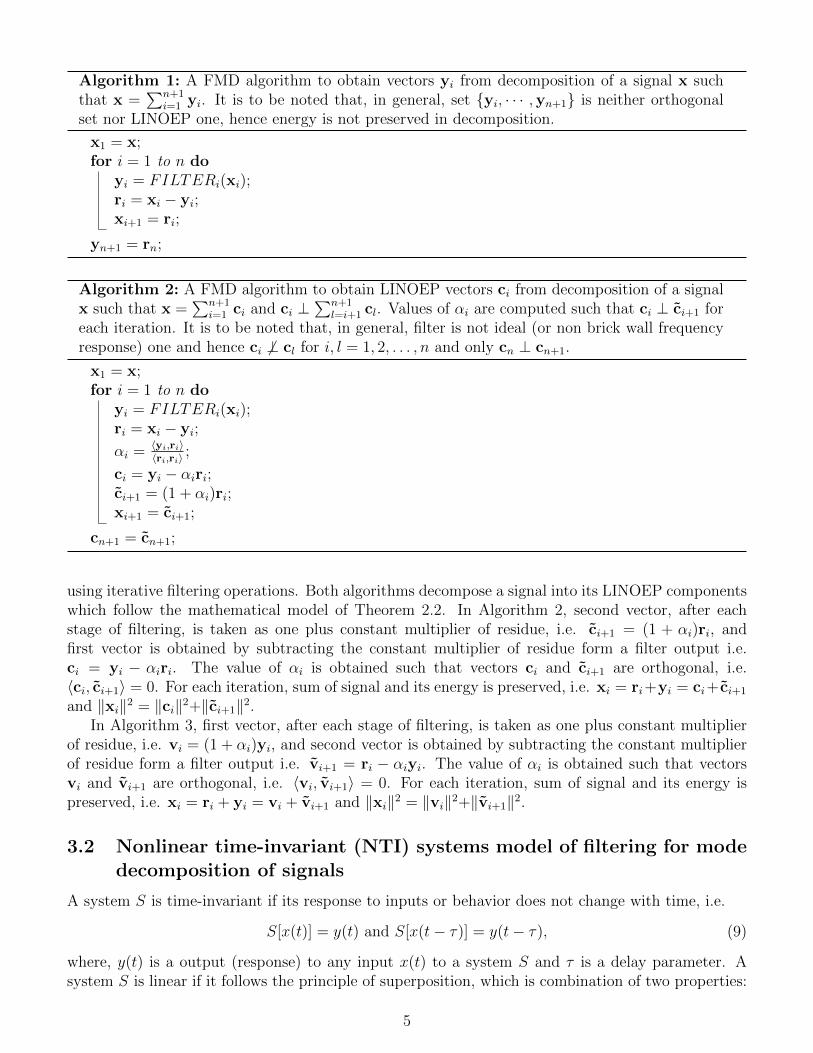
Algorithm 1: A FMD algorithm to obtain vectors yi from decomposition of a signal x suchthat x =

∑n+1i=1 yi. It is to be noted that, in general, set {yi, · · · ,yn+1} is neither orthogonal

set nor LINOEP one, hence energy is not preserved in decomposition.

x1 = x;for i = 1 to n do

yi = FILTERi(xi);ri = xi − yi;xi+1 = ri;

yn+1 = rn;

Algorithm 2: A FMD algorithm to obtain LINOEP vectors ci from decomposition of a signalx such that x =

∑n+1i=1 ci and ci ⊥

∑n+1l=i+1 cl. Values of αi are computed such that ci ⊥ ci+1 for

each iteration. It is to be noted that, in general, filter is not ideal (or non brick wall frequencyresponse) one and hence ci 6⊥ cl for i, l = 1, 2, . . . , n and only cn ⊥ cn+1.

x1 = x;for i = 1 to n do

yi = FILTERi(xi);ri = xi − yi;

αi = 〈yi,ri〉〈ri,ri〉 ;

ci = yi − αiri;ci+1 = (1 + αi)ri;xi+1 = ci+1;

cn+1 = cn+1;

using iterative filtering operations. Both algorithms decompose a signal into its LINOEP componentswhich follow the mathematical model of Theorem 2.2. In Algorithm 2, second vector, after eachstage of filtering, is taken as one plus constant multiplier of residue, i.e. ci+1 = (1 + αi)ri, andfirst vector is obtained by subtracting the constant multiplier of residue form a filter output i.e.ci = yi − αiri. The value of αi is obtained such that vectors ci and ci+1 are orthogonal, i.e.〈ci, ci+1〉 = 0. For each iteration, sum of signal and its energy is preserved, i.e. xi = ri+yi = ci+ ci+1

and ‖xi‖2 = ‖ci‖2+‖ci+1‖2.In Algorithm 3, first vector, after each stage of filtering, is taken as one plus constant multiplier

of residue, i.e. vi = (1 + αi)yi, and second vector is obtained by subtracting the constant multiplierof residue form a filter output i.e. vi+1 = ri − αiyi. The value of αi is obtained such that vectorsvi and vi+1 are orthogonal, i.e. 〈vi, vi+1〉 = 0. For each iteration, sum of signal and its energy ispreserved, i.e. xi = ri + yi = vi + vi+1 and ‖xi‖2 = ‖vi‖2+‖vi+1‖2.

3.2 Nonlinear time-invariant (NTI) systems model of filtering for modedecomposition of signals

A system S is time-invariant if its response to inputs or behavior does not change with time, i.e.

S[x(t)] = y(t) and S[x(t− τ)] = y(t− τ), (9)

where, y(t) is a output (response) to any input x(t) to a system S and τ is a delay parameter. Asystem S is linear if it follows the principle of superposition, which is combination of two properties:

5

Algorithm 3: A FMD algorithm to obtain LINOEP vectors vi from decomposition of a signalx such that x =

∑n+1i=1 vi and vi ⊥

∑n+1l=i+1 vl. Values of αi are computed such that vi ⊥ vi+1

for each iteration. It is to be noted that, in general, filter is not ideal one and hence vi 6⊥ vl fori, l = 1, 2, . . . , n and only vn ⊥ vn+1.

x1 = x;for i = 1 to n do

yi = FILTERi(xi);ri = xi − yi;

αi = 〈yi,ri〉〈yi,yi〉 ;

vi = (1 + αi)yi;vi+1 = ri − αiyi;xi+1 = vi+1;

vn+1 = vn+1;

homogeneity (scaling) and additivity, i.e. for any n signals {xl}nl=1 and any n scalars {al}nl=1,

S[ n∑l=1

alxl

]=

n∑l=1

alS[xl]. (10)

In words, linearity means scaling and summing before or after the system are the same for all theinput to output signal mappings. If a system S is not following the the principle of superposition,

then it is a nonlinear system, i.e. S[∑n

l=1 alxl

]6=∑n

l=1 alS[xl].

The EMD algorithm [1] can decompose a time series x(t) into a set of finite band-limited IMFsand residue, i.e. x(t) → EMD 7→ {y1(t), ..., yn(t), rn(t)} (or EMD[x(t)] = {y1(t), ..., yn(t), rn(t)}),such that the decomposed signal x(t) is the sum of IMF components {yi(t)}ni=1 and final residue rn(t):

x(t) =n∑k=1

yk(t) + rn(t) =n+1∑k=1

yk(t), (11)

where yk(t) is the kth IMF and rn(t) = yn+1(t). A set of IMFs obtained by EMD is neither orthogonalnor LINOEP vectors and, hence, energy of a signal is not preserved in decomposition. The energypreserving EMD (EPEMD) algorithm [7] decomposes a time series x(t) into a set of finite band-limitedIMFs and residue which follow the LINOEP vector model, i.e.

x(t) =n+1∑k=1

yk(t) and yk(t) ⊥n∑

l=k+1

yl(t). (12)

All IMFs must satisfy two basic conditions [1]: (1) In the complete range of time series, thenumber of extrema (i.e. maxima and minima) and the number of zero crossings are equal or differ atmost by one. (2) At any point of time, in the complete range of time series, the average of the valuesof upper and lower envelopes, obtained by the interpolation of local maxima and the local minima,is zero.

We observe that the EMD is following a nonlinear time-invariant (NTI) system model, and henceit is a iterative nonlinear time-invariant zero-phase filtering operations to decompose a signal intointrinsic mode functions (IMFs). All variants of the EMD algorithm are nonlinear because they don’t

6

follow the principle of superposition, i.e. there exist n signals {xl}nl=1:

EMD[ n∑l=1

xl

]6=

n∑l=1

EMD[xl]. (13)

Although it is easy to observe that EMD is a nonlinear system model, yet we provide counterexamplesto prove this fact.

Example 1: Let x1(t) = sin(10πt) and x2(t) = sin(100πt) in time interval 0 ≤ t ≤ 1 s. Clearly,both signal x1(t) and x2(t) are IMFs, ideally EMD[x1(t)] = x1(t) and EMD[x2(t)] = x2(t), thusEMD[x1(t)] + EMD[x2(t)] = x1(t) + x2(t). However, it is very easy to verify, by the all variants ofEMD algorithms, that ideally EMD[x1(t) + x2(t)] = {x1(t), x2(t)} which implies that EMD[x1(t) +x2(t)] 6= EMD[x1(t)] + EMD[x2(t)], i.e. {x1(t), x2(t)} 6= {x1(t) + x2(t)}. Clearly, EMD is a time-invariant system model as it follows (9), i.e. EMD[x1(t−τ)] = x1(t−τ), EMD[x2(t−τ)] = x2(t−τ)and EMD[x1(t− τ) + x2(t− τ)] = {x1(t− τ), x2(t− τ)}.

Example 2: Let xl(t) = (21 − l) sin(2πlf0t) for l = 1, 2, · · · , 20, in time interval, 0 ≤ t ≤ 1 s,with T0 = 1 = 1

f0. Clearly, all the xl(t) are IMFs and ideally EMD[xl(t)] = xl(t). However, it is very

easy to verify, by the all variants of EMD algorithms, that EMD[∑n

l=1 xl(t)]6=∑n

l=1EMD[xl(t)],

because EMD generates finite number of band-limited IMFs from the sum of all signals consideredin this example.

It is very interesting to note that above arguments along with equation (13) and Examples 1and 2 are valid for the other nonlinear and nonstationary time series analysis methods, such as syn-chrosqueezed wavelet transforms, variational mode decomposition, eigenvalue decomposition, Fourierdecomposition methods [4, 17], etc.

The FDM, entirely Fourier theory based decomposition, is recently proposed method [4] for thenonlinear and nonstationary time series analysis. The FDM algorithm can decompose a time seriesx(t) into a set of finite band-limited Fourier intrinsic band functions (FIBFs) and constant, i.e.x(t)→ FDM 7→ {y1(t), ..., yn(t), c} (or FDM [x(t)] = {y1(t), ..., yn(t), c}), such that the decomposedsignal x(t) is the sum of orthogonal FIBF components {yi(t)}ni=1 and a constant c:

x(t) =n∑k=1

yk(t) + c and 〈yk, c〉 = 〈yk, yl〉 = 0 for k 6= l, (14)

where yk(t) is the kth FIBF. The FIBFs, yk(t) ∈ C∞[a, b], are functions that satisfy the followingconditions [4]:

1. The FIBFs are zero mean functions, i.e.∫ bayk(t) dt = 0.

2. The FIBFs are orthogonal functions, i.e.∫ bayk(t)yl(t) dt = 0, for k 6= l.

3. The FIBFs provide analytic FIBFs (AFIBFs) with instantaneous frequency (IF) and amplitudealways greater than zero, i.e. yk(t) + jyk(t) = ak(t) exp(jφk(t)), with ak(t),

ddtφk(t) ≥ 0, ∀t.

Where, yk(t) is the Hilbert transform (HT) of FIBF yk(t), defined as convolution of yk(t) and 1/πt,

i.e. yk(t) = yk(t) ∗ 1πt

= 1π

p.v.∫∞−∞

yk(τ)t−τ dτ , where p.v. stands for the Cauchy principal value of the

integral. Even though the Hilbert transform is global, it emphasizes the properties of the functionat the local time t. Thus, the HT is used to examine and reveal the local properties of the functionyk(t) and hence x(t) in (14).

The FDM algorithm directly generate orthogonal vectors, whereas for other nonlinear and non-stationary time series analysis methods (e.g. EMD, SSWT, EVD, etc.), it is more natural to generate

7

LINOEP vectors as shown in Algorithm 2 and 3. From Algorithm 1, of course, one can generate(n + 1)! sets of orthogonal vectors form a set of (n + 1) LI vectors, {yi, · · · ,yn+1}, by using theGSOM (as a post processing).

4 Simulation and numerical results

In this section, we present the discrete spiral of Theodorus and some simulation results which provideinteresting properties of LINOEP vectors which have been obtained form linear time-invariant (LTI)zero-phase filtering operation on a signal.

4.1 The discrete spiral of Theodorus

We rewrite (2) and (3) as

k−1∑l=1

xl ⊥ xk, for k = 2, 3, · · · , n and x =n∑k=1

xk, n ∈ N. (15)

Then from the EPT Theorem 2.2, we obtain

‖x‖2 =

∥∥∥∥∥n∑k=1

xk

∥∥∥∥∥2

=n∑k=1

‖xk‖2. (16)

Now, if we take a set of 2D unit vectors {x1, · · · ,xn} which satisfy (15) (which means only first twovectors are orthonormal vectors, i.e. x1 ⊥ x2, and rest (n − 2) are LD unit vectors, i.e. they areobtained by the linear combinations of first two vectors), then we can define

Tl =l∑

k=1

xk, l = 1, 2, · · · , n. (17)

From (15) and (17), one can easily show that

Tl−1Tl = Tl −Tl−1 = xl, T1 = x1, Tl ⊥ xl+1, l = 1, 2, · · · , n; (18)

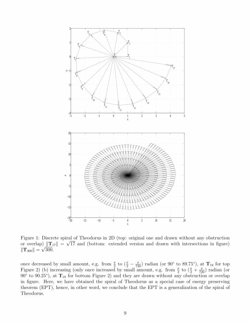
where T0 is the origin (zero vector). The discrete spiral of Theodorus is shown in Firure 1, whereT0 = [0 0]T . Let Φl is angle between T1 and Tl, then from Figure 1, we obtain angle between Tl+1

and Tl as

tan(Φl+1 − Φl) =1√l⇔ (Φl+1 − Φl) = tan−1

( 1√l

), Φ1 = 0, l = 1, 2, · · · , n. (19)

From above discussions and Figure 1, one can easily obtain

Tl =√l[cos(Φl) sin(Φl)]

T , T1 = x1 = [1 0]T , xl+1 = [− sin(Φl) cos(Φl)]T . (20)

and hence ‖Tl‖ =√l and ‖xl‖ = 1 (since xl are unit vectors).

This 2D discrete spiral of Theodorus can be extended to higher dimensions, using ND unit vectors(xl) such that it satisfy (15), (16), (17) and (18). For example, two discrete spiral of Theodorus areconstructed in 3D, as shown in Figure 2 with ‖T400‖ =

√400, using 3D unit vectors. It is interesting

to note that, angle between positive z-axis and Tl, for l ≥ 19, is automatically (a) decreasing (only

8

−3 −2 −1 0 1 2 3 4 5−4

−3

−2

−1

0

1

2

T1

x

y

T2

T3T

4T

5

T6

T7

T8

T9

T10

T11 T

12

T13

T14

T15

T16

T17

T0

−20 −15 −10 −5 0 5 10 15 20−20

−15

−10

−5

0

5

10

15

20

x

y

Figure 1: Discrete spiral of Theodorus in 2D (top: original one and drawn without any obstructionor overlap) ‖T17‖ =

√17 and (bottom: extended version and drawn with intersections in figure)

‖T300‖ =√

300.

once decreased by small amount, e.g. from π2

to (π2− π

720) radian (or 90◦ to 89.75◦), at T18 for top

Figure 2) (b) increasing (only once increased by small amount, e.g. from π2

to (π2

+ π720

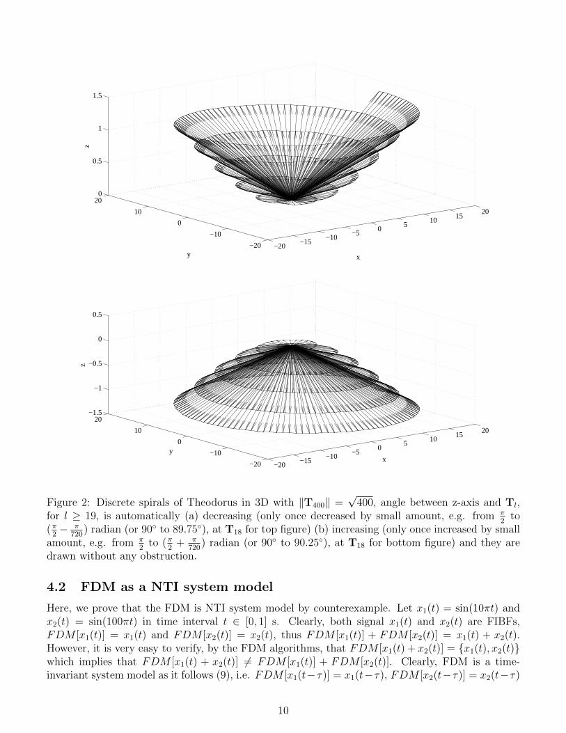
) radian (or90◦ to 90.25◦), at T18 for bottom Figure 2) and they are drawn without any obstruction or overlapin figure. Here, we have obtained the spiral of Theodorus as a special case of energy preservingtheorem (EPT), hence, in other word, we conclude that the EPT is a generalization of the spiral ofTheodorus.

9

−20−15

−10−5

05

1015

20

−20

−10

0

10

200

0.5

1

1.5

xy

z

−20−15

−10−5

05

1015

20

−20

−10

0

10

20−1.5

−1

−0.5

0

0.5

xy

z

Figure 2: Discrete spirals of Theodorus in 3D with ‖T400‖ =√

400, angle between z-axis and Tl,for l ≥ 19, is automatically (a) decreasing (only once decreased by small amount, e.g. from π

2to

(π2− π

720) radian (or 90◦ to 89.75◦), at T18 for top figure) (b) increasing (only once increased by small

amount, e.g. from π2

to (π2

+ π720

) radian (or 90◦ to 90.25◦), at T18 for bottom figure) and they aredrawn without any obstruction.

4.2 FDM as a NTI system model

Here, we prove that the FDM is NTI system model by counterexample. Let x1(t) = sin(10πt) andx2(t) = sin(100πt) in time interval t ∈ [0, 1] s. Clearly, both signal x1(t) and x2(t) are FIBFs,FDM [x1(t)] = x1(t) and FDM [x2(t)] = x2(t), thus FDM [x1(t)] + FDM [x2(t)] = x1(t) + x2(t).However, it is very easy to verify, by the FDM algorithms, that FDM [x1(t) + x2(t)] = {x1(t), x2(t)}which implies that FDM [x1(t) + x2(t)] 6= FDM [x1(t)] + FDM [x2(t)]. Clearly, FDM is a time-invariant system model as it follows (9), i.e. FDM [x1(t−τ)] = x1(t−τ), FDM [x2(t−τ)] = x2(t−τ)

10

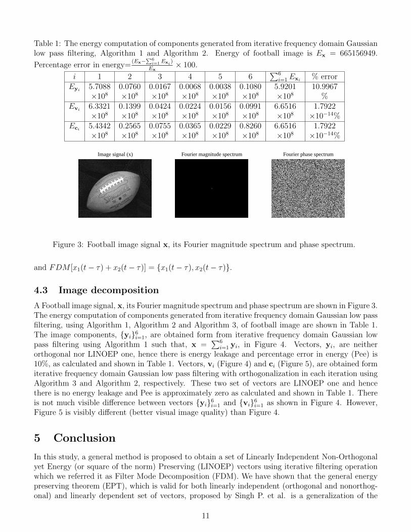
Table 1: The energy computation of components generated from iterative frequency domain Gaussianlow pass filtering, Algorithm 1 and Algorithm 2. Energy of football image is Ex = 665156949.

Percentage error in energy=(Ex−

∑6i=1 Exi )

Ex× 100.

i 1 2 3 4 5 6∑6

i=1Exi% error

Eyi5.7088 0.0760 0.0167 0.0068 0.0038 0.1080 5.9201 10.9967×108 ×108 ×108 ×108 ×108 ×108 ×108 %

Evi6.3321 0.1399 0.0424 0.0224 0.0156 0.0991 6.6516 1.7922×108 ×108 ×108 ×108 ×108 ×108 ×108 ×10−14%

Eci 5.4342 0.2565 0.0755 0.0365 0.0229 0.8260 6.6516 1.7922×108 ×108 ×108 ×108 ×108 ×108 ×108 ×10−14%

Image signal (x) Fourier magnitude spectrum Fourier phase spectrum

Figure 3: Football image signal x, its Fourier magnitude spectrum and phase spectrum.

and FDM [x1(t− τ) + x2(t− τ)] = {x1(t− τ), x2(t− τ)}.

4.3 Image decomposition

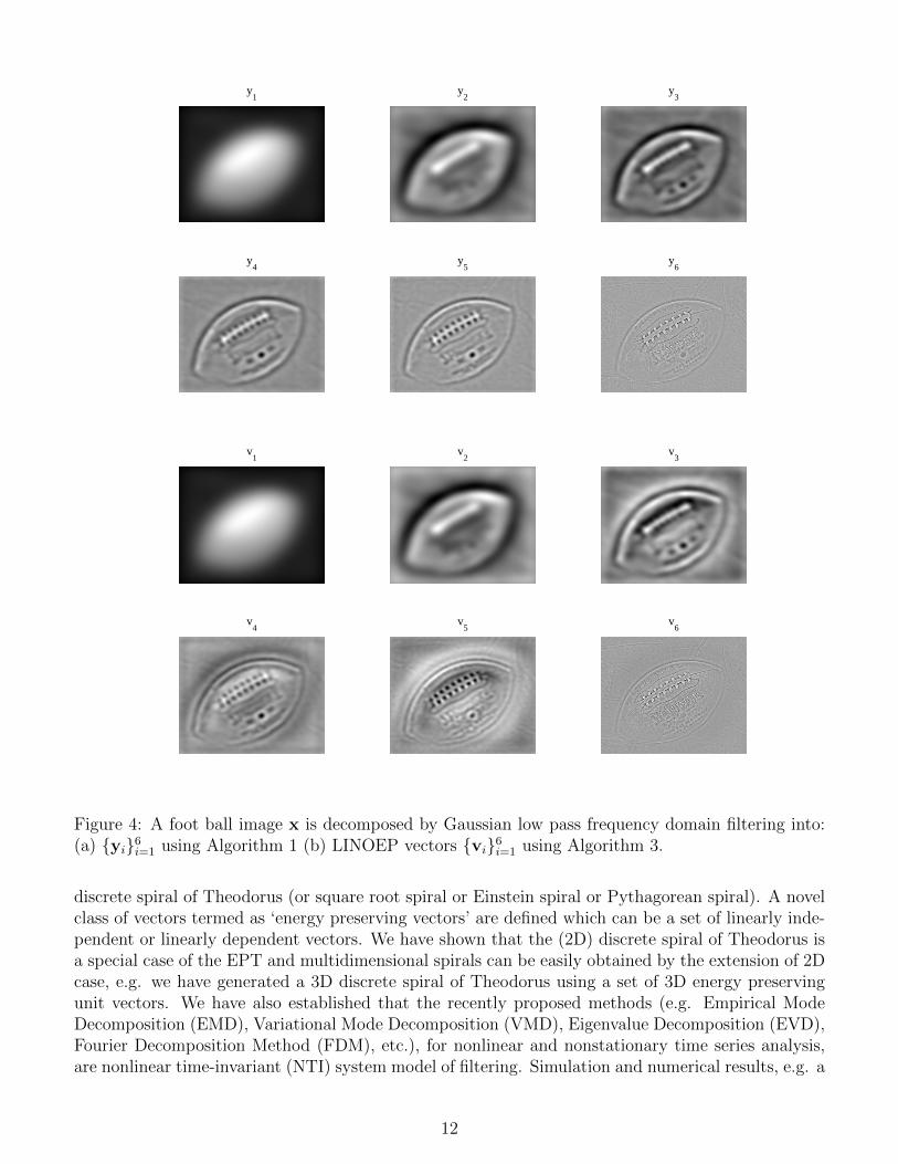
A Football image signal, x, its Fourier magnitude spectrum and phase spectrum are shown in Figure 3.The energy computation of components generated from iterative frequency domain Gaussian low passfiltering, using Algorithm 1, Algorithm 2 and Algorithm 3, of football image are shown in Table 1.The image components, {yi}6i=1, are obtained form from iterative frequency domain Gaussian lowpass filtering using Algorithm 1 such that, x =

∑6i=1 yi, in Figure 4. Vectors, yi, are neither

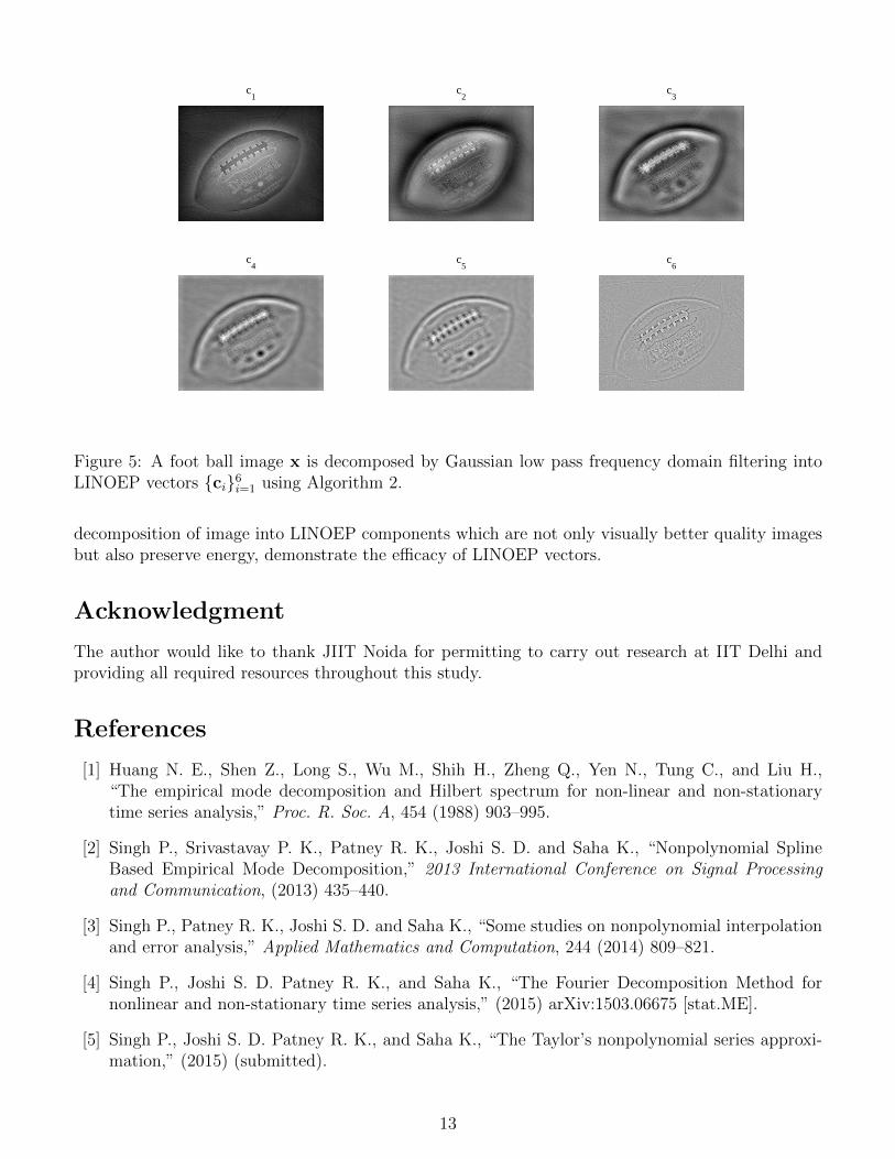
orthogonal nor LINOEP one, hence there is energy leakage and percentage error in energy (Pee) is10%, as calculated and shown in Table 1. Vectors, vi (Figure 4) and ci (Figure 5), are obtained formiterative frequency domain Gaussian low pass filtering with orthogonalization in each iteration usingAlgorithm 3 and Algorithm 2, respectively. These two set of vectors are LINOEP one and hencethere is no energy leakage and Pee is approximately zero as calculated and shown in Table 1. Thereis not much visible difference between vectors {yi}6i=1 and {vi}6i=1 as shown in Figure 4. However,Figure 5 is visibly different (better visual image quality) than Figure 4.

5 Conclusion

In this study, a general method is proposed to obtain a set of Linearly Independent Non-Orthogonalyet Energy (or square of the norm) Preserving (LINOEP) vectors using iterative filtering operationwhich we referred it as Filter Mode Decomposition (FDM). We have shown that the general energypreserving theorem (EPT), which is valid for both linearly independent (orthogonal and nonorthog-onal) and linearly dependent set of vectors, proposed by Singh P. et al. is a generalization of the

11

y1

y2

y3

y4

y5

y6

v1

v2

v3

v4

v5

v6

Figure 4: A foot ball image x is decomposed by Gaussian low pass frequency domain filtering into:(a) {yi}6i=1 using Algorithm 1 (b) LINOEP vectors {vi}6i=1 using Algorithm 3.

discrete spiral of Theodorus (or square root spiral or Einstein spiral or Pythagorean spiral). A novelclass of vectors termed as ‘energy preserving vectors’ are defined which can be a set of linearly inde-pendent or linearly dependent vectors. We have shown that the (2D) discrete spiral of Theodorus isa special case of the EPT and multidimensional spirals can be easily obtained by the extension of 2Dcase, e.g. we have generated a 3D discrete spiral of Theodorus using a set of 3D energy preservingunit vectors. We have also established that the recently proposed methods (e.g. Empirical ModeDecomposition (EMD), Variational Mode Decomposition (VMD), Eigenvalue Decomposition (EVD),Fourier Decomposition Method (FDM), etc.), for nonlinear and nonstationary time series analysis,are nonlinear time-invariant (NTI) system model of filtering. Simulation and numerical results, e.g. a

12

c1

c2

c3

c4

c5

c6

Figure 5: A foot ball image x is decomposed by Gaussian low pass frequency domain filtering intoLINOEP vectors {ci}6i=1 using Algorithm 2.

decomposition of image into LINOEP components which are not only visually better quality imagesbut also preserve energy, demonstrate the efficacy of LINOEP vectors.

Acknowledgment

The author would like to thank JIIT Noida for permitting to carry out research at IIT Delhi andproviding all required resources throughout this study.

References

[1] Huang N. E., Shen Z., Long S., Wu M., Shih H., Zheng Q., Yen N., Tung C., and Liu H.,“The empirical mode decomposition and Hilbert spectrum for non-linear and non-stationarytime series analysis,” Proc. R. Soc. A, 454 (1988) 903–995.

[2] Singh P., Srivastavay P. K., Patney R. K., Joshi S. D. and Saha K., “Nonpolynomial SplineBased Empirical Mode Decomposition,” 2013 International Conference on Signal Processingand Communication, (2013) 435–440.

[3] Singh P., Patney R. K., Joshi S. D. and Saha K., “Some studies on nonpolynomial interpolationand error analysis,” Applied Mathematics and Computation, 244 (2014) 809–821.

[4] Singh P., Joshi S. D. Patney R. K., and Saha K., “The Fourier Decomposition Method fornonlinear and non-stationary time series analysis,” (2015) arXiv:1503.06675 [stat.ME].

[5] Singh P., Joshi S. D. Patney R. K., and Saha K., “The Taylor’s nonpolynomial series approxi-mation,” (2015) (submitted).

13

[6] Singh P., Joshi S. D., Patney R. K., and Saha K., “Fourier based feature extraction for classifi-cation of EEG signals using EEG rhythms,” (2015) (submitted).

[7] Singh P., Patney R. K., Joshi S. D. and Saha K., “The Hilbert spectrum and the EnergyPreserving Empirical Mode Decomposition,” (2015) arXiv:1504.04104v1 [cs.IT].

[8] Singh P., Joshi S. D. Patney R. K., and Saha K., “The Linearly Independent Non Orthogonalyet Energy Preserving (LINOEP) vectors,” (2014) arXiv:1409.5710 [math.NA].

[9] Daubechies I., Lu J., Wu H. T., “Synchrosqueezed Wavelet Transforms: an Empirical ModeDecomposition-like Tool,” Appl. Comput. Harmon. Anal., 30 (2011) 243–261.

[10] Dragomiretskiy K., Zosso D., “Variational Mode Decomposition,” IEEE Transactions on SignalProcessing, 62(3) (2014) 531–544.

[11] P. Jain, R. B. Pachori, “An iterative approach for decomposition of multi-componentnon-stationary signals based on eigenvalue decomposition of the Hankel matrix,” Journal of theFranklin Institute (2015), http://dx.doi.org/10.1016/j.jfranklin.2015.05.038.

[12] Gautschi W., “The spiral of Theodorus, numerical analysis, and special functions,” Journal ofComputational and Applied Mathematics, 235 (2010) 1042–1052.

[13] Davis P. J., “Spirals: From Theodorus to Chaos,” A. K. Peters, 1993.

[14] Gautschi W., “The spiral of Theodorus, special functions, and numerical analysis,” In P.J. Davis,op. cit., 67–87.

[15] Jorg Waldvogel, “Analytic Continuation of the Theodorus Spiral,” Seminar fur AngewandteMathematik, ETH Zurich, October 9, 2008 to February 2009.

[16] Hahn H. K., Kay Schoenberger, “The Ordered Distribution of Natural Numbers on the SquareRoot Spiral,” arXiv:0712.2184 [math.GM].

[17] Singh P., Joshi S. D., “Some studies on multidimensional Fourier theory for Hilbert transform,analytic signal and space-time series analysis,” (2015) arXiv:1507.08117 [cs.IT].

14