Embed Size (px)
Citation preview

The Pennsylvania State University
The Graduate School
College of Liberal Arts
LINKING TASK-MODULATED FUNCTIONAL CONNECTIVITY TO INDIVIDUAL
DIFFERENCES IN BEHAVIOR: THE CASE OF FACE PROCESSING
A Thesis in
Psychology
by
Daniel B. Elbich
© 2016 Daniel Elbich
Submitted in Partial Fulfillment
of the Requirements
for the Degree of
Master of Science
August 2016

ii
The thesis of Daniel Elbich was reviewed and approved* by the following:
K. Suzanne Scherf Assistant Professor of Psychology Thesis Advisor Ping Li Professor of Psychlogy and Linguistics Koraly Perez-Edgar Associate Professor of Psychology Peter C.M. Molenaar Distinguished Professor of Human Development and Family Studies Melvin Mark Professor of Psychology Head of the Department of Psychology
*Signatures are on file in the Graduate School

iii
ABSTRACT
The study of the brain is currently undergoing a critical transition from the study of
individual regions to the study of connectivity between regions. In this newly emerging focus on
how the brain functions as a network, a network is represented by a series of regions (nodes) and
the connections between them (edges). One domain in which the network level approach has
made great strides is in face-processing, but there still many important questions remaining with
regards to how individual differences in connectivity relate to differences in face-processing
behaviors. In this project, I used state-of-the art connectivity methods to address the following
questions: 1) is variation in face recognition behavior related to variation in the topologic
organization of the face-processing network, 2) how do the relation between network
organization and behavior change when viewing faces versus other visual objects? I behavioral
tested and scanned 40 adult participants, measuring face and object recognition ability and brain
responses to faces. I conducted effective connectivity analyses to determine the network topology
of the full face-processing network (core and extended) during face, object, and place viewing at
3 levels of analysis. Finally these topologies were quantified using Graph Theoretical Metrics and
Pattern Recognition analyses. The results show that as face recognition ability increases, the PCC
and bilateral Amygdala become less hub-like within the network. Additionally, the vmPFC
becomes an inter-modular hub as face recognition increases. Finally, superior face recognizers
exhibit more unique network topologies during face viewing compared to object viewing, while
average and low recognizers do not. These results show that not only do high performers have
fewer and more direct connections, resulting in more compact network topologies, but also that
these topologies are specific to viewing faces and not other visual categories. Further, high
performers networks when viewing faces are organized differently than when viewing objects,
but such is not the case for average or low recognizers. This research is the first of its kind to

iv
merge effective connectivity, graph theory, and pattern recognition to study individual differences
in network topology.

v
TABLE OF CONTENTS
LIST OF FIGURES…………………………………………………………………….….………v
LIST OF TABLES………………………………………………………………………….….….vi
ACKNOWLEDGEMENTS………………………………………………………..……………...ix
Chapter 1 Introduction………………………………………………………….………………….1 Face Processing Network………………….……………………………………..……….3 Functional Connectivity..………………….……………………………………..……….4 Directional/Effective Connectivity……….……………………………………..………...5 Current Project….……………………..……………………………..……………….….10 Chapter 2 Method………………………………………………………….……………………..12 General Methodology………………….……………………………………..………….12
Participants…………………….………………………………...……..………….12 Behavioral Measures…………………….……………………………………..….13 Neuroimaging Protocol………………….……………………………………..….15 Data Analysis………...………………….……………………………………..….16
Task-Related Network Modulation….………………….……………..……..….……….19 Graph Theory Metrics………………….……………………………………..………….19 Pattern Recognition………………….……………………………………..…………….22 Analysis Strategy………………….……………………………………..………………24
Chapter 3 Results………………………………………………………….……………………...26 Single Group Model..………………….……………………………………...………….26
Individual Model…………………….………………….……………..……..….……….27 Multiple Group Model……...………….……………………………………..………….30
Brain-Behavior Relations……………….………………………………….…..….33 Pattern Recognition………………….……………………………………..…………….38
Chapter 4 Discussion..…………………………………………………….……………………...93 Face Network and Visual Category..……………… ………………………...………….93
Modeling Methodology.…………….………………….……………..……..….……….98 Variation in Connectivity Patterns……...………….………………………...…………101 Conclusion………………….……………………………………..……………………102
Appendix Figure Legends..………………...…………………………….……………………...103 References..………………………………...…………………………….……………………...107

vi
LIST OF FIGURES Figure 1: Example network structure………………………………………………………………2
Figure 2: Example items from each of the behavioral tasks……………………………….……..14
Figure 3: Connection Path Matrices. Sample connection matrices of 2 subjects while viewing faces……………………………………………..…………………………..……..20
Figure 4: Vectorizing Beta Matrix………………………………………………………………..23
Figure 5: Relationships Between Face Recognition Tasks and Graph Theory Metrics in Single Group Model………………………………………………………………….……..27
Figure 6: Relationships Between Face Recognition Tasks and Graph Theory Metrics in Individual Group Model………………………..………………………………….………..29
Figure 7: Group Differences in Separate Model Analysis………………………………………..32
Figure 8: Relationships Between Face Recognition Tasks and Global Graph Theory Metrics in Multiple Group Model……………………………………….…………………..33
Figure 9: Relationships Between Face Recognition Tasks and vmPFC & PCC Graph Theory Metrics in Multiple Group Model………………………………………………….………..34
Figure 10: Relationships Between Face Recognition Tasks and Amygdale Graph Theory Metrics in Multiple Group Model……………………………………..………………….....36
Figure 11: Relationships Between Face Recognition Tasks and Graph Theory Metrics in Multiple Group Model…………………………………………………….........……….…..37
Figure 12: Connection Matrices for Face & Object Viewing in Separate Group Model………...##
Figure 13: Matrix representation of common connections during face viewing generated from Single Group and Individual Models………………………………………………………..##

vii
LIST OF TABLES Table 1: Subject Demographics and Behavioral Scores…….………….……...……..…………..12
Table 2: Summary Coordinates of Regions of Interest…….….……………...…………………..18
Table 3: Description of Graph Theory Metrics & Network Characteristics……………….……..21
Table 4: Relationship Between Behavioral Measures and Global Graph Theory Metrics in Single Group Model…….…………………………...…..…….……….……….…………………..40
Table 5: Relationship Between Behavioral Measures and Centrality in Single Group Model for
Face Viewing………………………………………………………………………………..41 Table 6: Relationship Between Behavioral Measures and Centrality in Single Group Model for
Object Viewing………………………………………………………………….…………..42 Table 7: Relationship Between Behavioral Measures and Centrality in Single Group Model for
Place Viewing………….………………………………………………….………….……..43 Table 8: Relationship Between Behavioral Measures and Clustering Coefficient in Single Group
Model for Face Viewing……………………………………..…………….………………..44 Table 9: Relationship Between Behavioral Measures and Clustering Coefficient in Single Group
Model for Object Viewing…………………………………………………………………..45 Table 10: Relationship Between Behavioral Measures and Clustering Coefficient in Single Group
Model for Place Viewing………….……………………………….………………………..46 Table 11: Relationship Between Behavioral Measures and Diversity in Single Group Model for
Face Viewing……………………………………..…………………….….………………..47 Table 12: Relationship Between Behavioral Measures and Diversity in Single Group Model for
Object Viewing……………………………………………………………….……………..48 Table 13: Relationship Between Behavioral Measures and Diversity in Single Group Model for
Place Viewing………….……………………………….………………….………………..49 Table 14: Relationship Between Behavioral Measures and Connection Strength Total in Single
Group Model for Face Viewing……………………………………..…………………..…..50 Table 14: Relationship Between Behavioral Measures and Connection Strength Total in Single
Group Model for Object Viewing…………………………………………………………..51 Table 16: Relationship Between Behavioral Measures and Connection Strength Total in Single
Group Model for Place Viewing………….……………………………….………………..52 Table 17: Relationship Between Behavioral Measures and Global Graph Theory Metrics in
Individual Model…….……………………....…..…….……….……….…………………..53

viii
Table 18: Relationship Between Behavioral Measures and Centrality in Individual Model for Face Viewing………………….…………………………..……………………….………..54
Table 19: Relationship Between Behavioral Measures and Centrality in Individual Model for
Object Viewing……………………..……………………..………………………….……..55 Table 20: Relationship Between Behavioral Measures and Centrality in Individual Model for
Place Viewing………….……………………………..……..…………….…………….…..56 Table 21: Relationship Between Behavioral Measures and Clustering Coefficient in Individual
Model for Face Viewing……………………………..…………………….………………..57 Table 22: Relationship Between Behavioral Measures and Clustering Coefficient in Individual
Model for Object Viewing…………………………………………………………………..58 Table 23: Relationship Between Behavioral Measures and Clustering Coefficient in Individual
Model for Place Viewing………….……………………………….………………………..59 Table 24: Relationship Between Behavioral Measures and Diversity in Individual Model for Face
Viewing………………………………...……………………………….….………………..60 Table 25: Relationship Between Behavioral Measures and Diversity in Individual Model for
Object Viewing………………….…………………………...……………….……………..61 Table 26: Relationship Between Behavioral Measures and Diversity in Individual Model for
Place Viewing………….………………………….……………………….………………..62 Table 27: Relationship Between Behavioral Measures and Connection Strength Total in
Individual Model for Face Viewing……………………………………….…………….…..63 Table 28: Relationship Between Behavioral Measures and Connection Strength Total in
Individual Model for Object Viewing…………………………………..…………………..64 Table 29: Relationship Between Behavioral Measures and Connection Strength Total in
Individual Model for Place Viewing………….………………….…………..……………..65 Table 30: ANOVA of Global Graph Theory Metrics across All Models………………………..66
Table 31: ANOVA of Node Centrality in Face Viewing………………………………………...67
Table 32: ANOVA of Node Centrality in Object Viewing……………………….……………...68
Table 33: ANOVA of Node Centrality in Place Viewing………………………………...……...69
Table 34: ANOVA of Node Clustering Coefficient in Face Viewing…………………….……...70
Table 35: ANOVA of Node Clustering Coefficient in Object Viewing………..………………...71
Table 36: ANOVA of Node Clustering Coefficient in Place Viewing…………………………...72
Table 37: ANOVA of Node Diversity in Face Viewing………………………………..………...73

ix
Table 38: ANOVA of Node Diversity in Object Viewing…………………………..…………...74
Table 39: ANOVA of Node Diversity in Place Viewing………………………………………...75
Table 40: ANOVA of Node Total Connection Strength in Face Viewing………………..……...76
Table 41: ANOVA of Node Total Connection Strength in Object Viewing………………...…...77
Table 42: ANOVA of Node Total Connection Strength in Place Viewing……………….……...78
Table 43: Relationship Between Behavioral Measures and Global Graph Theory Metrics in Separate Model…….…………………...…....…..…….……….……….…………………..79
Table 44: Relationship Between Behavioral Measures and Centrality in Separate Model for Face
Viewing………………….…………………………..…………………….………….……..80 Table 45: Relationship Between Behavioral Measures and Centrality in Separate Model for
Object Viewing……………………..……………………..………………….……………..81 Table 46: Relationship Between Behavioral Measures and Centrality in Separate Model for Place
Viewing………….……………………………..……..…………….……………...………..82 Table 47: Relationship Between Behavioral Measures and Clustering Coefficient in Separate
Model for Face Viewing……………………………..…………………….………………..83 Table 48: Relationship Between Behavioral Measures and Clustering Coefficient in Separate
Model for Object Viewing…………………………………………………………………..84 Table 49: Relationship Between Behavioral Measures and Clustering Coefficient in Separate
Model for Place Viewing………….……………………………….………………………..85 Table 50: Relationship Between Behavioral Measures and Diversity in Separate Model for Face
Viewing………………………………...……………………………….….………………..86 Table 51: Relationship Between Behavioral Measures and Diversity in Separate Model for Object
Viewing………………….…………………………...……………….……………………..87 Table 52: Relationship Between Behavioral Measures and Diversity in Separate Model for Place
Viewing………….………………………….……………………….……………….….…..88 Table 53: Relationship Between Behavioral Measures and Connection Strength Total in Separate
Model for Face Viewing……………………………………….………………………..…..89 Table 54: Relationship Between Behavioral Measures and Connection Strength Total in Separate
Model for Object Viewing…………………………………..…………………………..…..90 Table 55: Relationship Between Behavioral Measures and Connection Strength Total in Separate
Model for Place Viewing………….………………….…………..…………………………91 Table 56: Pattern Similarity for Separate Model Comparison Between Faces, Objects, and
Places…………………………………………………………………………………….….92

x
ACKNOWLEDGEMENTS
I would like to thank my advisor, Dr. Suzy Scherf, for all her advise and counsel on the project
and her invaluable mentorship of my graduate training. I would also like to thank the members of
my committee, Ping Li, Koraly Perez-Edgar, and Peter Molenaar, for their invaluable feedback
and advice. I would also like to give many thanks to my colleagues in the Lab of Developmental
Neuroscience, Lisa Whyte, Giorgia Picci, Natalie Motta-Mena, and Sara Barth, for their help with
feedback and assistance you have given me along the way. I would also like to thank all of the
undergraduate research assistants for your help in collecting the data used I this project. Finally, I
would like to thank my wonderful family for their continued support.

1
Chapter 1
Introduction
The study of the brain is currently undergoing a critical transition. Historically, much of
brain science has focused on identifying specific one-to-one mappings between brain structure
and function. Initially, the best and only way to study these mappings was based on the
histological examination of the injured or diseased brain. For example, scientists examined the
effects of strokes or acquired lesions on particular neural regions that resulted in severe and
seemingly selective deficits such as aphasia (loss of normal speech production) from lesions to
Broca’s area (Kean, 1977) and prosopagnosia (the inability to recognize faces while maintaining
spared object recognition abilities) from lesions to the fusiform gyrus (Meadows, 1974). These
findings lead to strong conclusions that specific brain regions are necessary for particular
behaviors and mental functions. The critical shift in this kind of thinking began with the advent of
newer technology, including functional magnetic resonance imaging (fMRI), which enabled in
vivo methodologies to address questions about brain function. However, the original questions
driving the use of this technology to evaluate the relation between brain structure and function
were embedded in this early perspective: which neural regions are responsible for which
behaviors?
Initially cognitive neuroscientists used fMRI to map the landscape of the brain by
observing which areas of the brain activated more strongly to one condition compared to another
in a given task (Bandettini, 2012; Puce et al., 1995). Consistently, researchers found that
performance on most tasks was supported not by a single or even small set of neural regions, but
by a diffuse set of areas that were widely distributed across the brain (e.g., Haxby et al., 2000;
Bandettini, 2012). For example, although lesions studies suggested that Broca’s and Wernickie’s
areas in the left hemisphere would be the prominent language areas in the brain, fMRI studies
revealed that there are a large number of regions that support language processing (see Price,

2
2012 for review). These kinds of findings lead researchers to begin thinking about the brain as a
distributed system of networks rather than a conglomeration of isolated individual regions. There
was a growing interest in understanding how the brain integrates information across networks of
distributed regions (Friston, 2011).
At the turn of the century, this new network perspective about the relation between brain
function and structure became prominent (Sporns et al., 2000). Researchers began to think about
how to characterize the brain by its connections rather than the individual regions. For example,
there are only a finite number of regions within the brain that can be parsed and attributed a
specific function. However, the idea began to form that behavior emerges from the interaction
and integration of these regions. As a result, a single network of regions could permute into
multiple different organizational profiles, each giving rise to a different behavior.
In this perspective, a network is represented by a series of regions (nodes) and the
connections between them (edges; see Figure 1). In brain science, nodes range from single
neurons to anatomical structures to functional regions. This makes node selection an important
first step in both creating and understanding a network, as this will drastically alter inferences
made about the network.
Figure 1: Example network structure

3
The edges within a network provide information about connections between nodes, which
can be quantified to provide information about the structure and community organization among
the nodes. For example, one characteristic about nodes is that they can be hubs, a central area that
is connected to a large portion of other nodes in the network. In functional brain networks, hubs
play a key role in the network and to a larger extent behavior (Buckner et al., 2009). Additionally,
groups of nodes can be organized into modules, or sets of nodes that maximize within-group
edges and minimize between-group edges (Leicht & Newman, 2008). Modular organization
reflects smaller portions of the network that co-activate to accomplish part of a process (Bullmore
& Sporns, 2009).
Face Processing Network
One domain in which the network level approach has made great strides is in face-
processing. One of the most well known early fMRI findings about the neural basis of face-
processing was reported by Kanwisher and colleagues (1997), who reported about the fusiform
face area (FFA; Kanwisher et al., 1997). The FFA is a functional region located in the fusiform
gyrus that preferentially activates to faces over other categories of visual stimuli (Kanwisher et
al., 1997). This neuroimaging finding built on previous patient work suspecting the importance of
the fusiform gyrus for face-processing (De Renzi, 1977). Findings of the circumscribed FFA
resonated strongly in the literature and sparked hundreds of studies interrogating exactly how this
region supports face processing.
However, Haxby and colleagues (2000) proposed a model of face-processing suggesting
that multiple disparate neural regions, not just the FFA, are critically involved in the processing
of recognizing faces and extracting information expressed on faces (Haxby et al., 2000). This
model delineates a ‘core’ set of neural regions comprised of the fusiform gyrus (FFA), inferior
occipital gyrus (OFA), and posterior superior temporal sulcus (pSTS), as well as ‘extended’
regions such as the amygdala and anterior temporal pole (Haxby et al., 2000). This model has

4
gained increasing support. For example, Avidan and colleagues (2005) examined how the FFA
functions in subjects with a congenital version of prosopagnosia (CP), in which individuals have
face blindness in the absence of any neurological damage (Avidan et al., 2005). They had a strong
prediction that the FFA would not be active in CPs, based on findings from acquired
prosopagnosics. However, to the astonishment of the researchers and the field, they found that
CPs have normal levels of activation in the FFA in response to faces (Avidan et al., 2005). This
finding challenged the idea that the FFA is sufficient for face processing and shifted the focus
toward examining the functional network topology underlying face processing.
The Haxby and colleagues (2000) model has expanded to encompass even more regions
as additional evidence for this network model became available (Gobbini & Haxby, 2007).
Additionally, non-human primate work in this domain shows that the macaque visual system not
only shares commonalities with the human visual system (Tsao et al., 2008; Pinsk et al., 2009),
but also has multiple face-sensitive patches (Moeller et al., 2008). Thus, there is a growing body
of convergent evidence from human and non-human fMRI research that there are multiple
regions that are consistently activated when individuals process faces. Additionally, the last
decade has begun to show that these regions function together as a cohesive network, in that they
are temporally synchronous in their patterns of activation during face-processing tasks (Fairhall &
Ishai, 2007; Avidan et al. 2014; Hahamy et al. 2015; Joseph et al., 2012; O’Neil et al., 2014). In
other words, they exhibit evidence of functional connectivity.
Functional Connectivity
Functional connectivity refers to the temporal synchrony in activation between discrete
regions in the brain. This idea relies on the principle of Hebbian Learning, which stipulates that
neurons that fire together wire together (Hebb, 1949). In order to argue that a set of neural regions
functions as an integrated neural network, functional connectivity among the regions must be
established. Otherwise, there is no clear evidence of integrated function across the regions.

5
Multiple methodologies have been designed to assess connectivity within neural
networks including correlational analyses and effective (i.e., directed functional) connectivity
approaches such as Dynamic Causal Modeling (DCM; Friston et al., 2003), Granger Causality
(GCM; Goebel et al., 2003), Structural Equation Modeling (SEM; Friston, 2011), and unified
Structural Equation Modeling (uSEM; Kim et al., 2007). These methods have undergone rapid
evolution, starting with simple correlational approaches and extending into incredibly complex
modeling procedures that seek to characterize the functional and effective connectivity between
regions of the brain. The methods all test the concept that regions within a network exhibit
temporally coordinated activation. Correlations analyses evaluate the strength of the
contemporaneous temporal synchrony of response profiles between pairs of regions across the
timecourse of the experimental paradigm. Effective connectivity analyses evaluate the directional
flow of information between pairs of regions by estimating the predictive (lagged) effect of one
region on another (i.e., activity in one region at one time predicts activation in another region at
the next time point in the series).
One of the most common approaches for evaluating functional connectivity utilizes a
point-by-point correlational analysis on the raw timecourse data from pairs of neural regions.
Specifically, across participants, an average correlation is estimated for each time point in the
timecourse between the two regions. A higher average correlation coefficient indicates stronger
temporal co-activation between the regions across participants and is taken as evidence of
functional connectivity between regions. In this approach, for example, a timecourse of one
region (e.g. FFA) is correlated to timecourses for each of the other neural regions within the
network (i.e. one to many). The results in can be represented in a matrix of correlations
coefficients of all possible pairs.
This approach has been used to assess functional connectivity in the neural circuitry of
multiple cognitive domains, including face recognition (Avidan et al. 2014; Hahamy et al. 2015;
Joseph et al., 2012; O’Neil et al., 2014). For example, Avidan and colleagues (2014) found that

6
subjects with prosopagnosia had increased functional connectivity between amygdala and core
face-processing regions, but decreased connectivity between core regions and the anterior
temporal pole (ATP), a region that is implicated in storing invariant representations of faces
(Kriegeskorte et al., 2007; Avidan et al. 2014). Thus, correlational analyses can be helpful for
examining temporal co-activation between pairs of regions and potential differences between
participant groups in the strength of these connections between regions. However, because the
nature of the computation is correlational, the directionality of the connection cannot be
determined, nor can the nature of the influence of the connection (direct, indirect, shared) and this
approach is limited to characterizing connections between pairs of regions; it does not provide
any information about how regions interact in a more global context.
A solution to this problem has been to borrow graph theory metrics from network science
as a way to quantify the topologic organization of complex functional neural networks (not just
pairs of connections) (Rubinov & Sporns, 2010; Bassett & Lynall, 2013). In its adaptation to
systems neuroscience, graph theory is a computational methodology that characterizes different
properties of neural networks, as in the global, local, and nodal properties. For example, global
properties entail large-scale characteristics (e.g., number of total connections), local properties
comprise smaller neighborhood characteristics (e.g., nodes which cluster around a particular
node), and nodal properties that describe the role of nodes in the network architecture (e.g., hub
properties). These properties are useful for quantifying differences in network architecture and
relative importance of an individual node or set of nodes within the architecture. While graph
theory metrics were originally used to study anatomical connections in the brain, these metrics
have recently been used more to characterize functional networks as well (Bullmore & Sporns,
2009; van Wijk et al., 2010).
The correlational approach has been also used to evaluate how task conditions modulate
profiles of functional connectivity. A version of this approach is called the psychophysiological
interaction (PPI) approach and was proposed by Friston et al., (1997). The original proposal was

7
to create a regressor that models the interaction between the raw timecourse from a region (i.e.
right FFA) and the task. However, in order for the regressor to reflect neural activity at each
timepoint of the experimental paradigm (which would otherwise be smeared out in the raw fMRI
data), the underlying neuronal signal must be estimated from the observed fMRI signal using
deconvolution (Gitelman et al., 2003). The regressor is then included with the original general
linear model and used to locate other voxels that exhibit a similar interaction. This PPI method
enables the identification of a set of regions that are similarly modulated by the task, but it is
limited in that it cannot identify the directional flow of information between any of the regions.
Additionally, this method is specifically designed to identify areas of a network, not to understand
modulations in the organization of connections among a priori defined nodes in a network.
Directional/Effective Connectivity
While discovering connections between regions is valuable, the directionality of the
connections is crucial to understanding the actual topologic organization of the network (e.g. flow
of information). The common approaches to measuring effective connectivity, DCM, GCM, and
SEM involve modeling directional connections between regions. In other words, in additional to
evaluating whether there is temporal co-activation between any two regions, these approaches
investigate the directional flow of information between the regions by estimating the directed
(lagged) connections.
DCM was specifically designed to model causal relations (using contemporaneous
connections) in neuroimaging data (Friston et al., 2003). In this approach, all models being tested
are defined a priori, making this approach more hypothesis driven (Friston et al., 2003).
Additionally, because DCM tests directionality, the direction of the connection within the tested
model matters greatly to choosing appropriate models (i.e. different direction equals different
model). Using a Bayesian modeling approach, all models are tested for each subject to determine
the best model fit for the given data (Friston et al., 2003). The “best” model is the one that the
majority of participants fit (i.e. winner take all). For example, Fairhall & Ishai (2007) showed that

8
a feed-forward approach best describes regions in the core part of the face-processing network, in
that information from the OFA directly connects to both the pSTS and FFA (Fairhall & Ishai,
2007). However, there are limitations of the DCM approach. This method can only model
contemporaneous connections, and thus cannot infer direct connections in the across time space.
Additionally, DCM lacks the ability to search for all possible topologies (Smith et al., 2011).
GCM is a different approach to DCM in that it only models lagged connections (Goebel
et al., 2003). Additionally, instead of being constrained by a priori model selection, it is
conducted at the whole brain level (Goebel et al., 2003). GCM is more suited for forecasting
timecourse data, meaning determining how well data in one region at one timepoint can predict
the timecourse from another region later in time (Goebel et al., 2003). In essence, timecourse data
from multiple regions are fit to an autoregressive model in order to determine if signal changes in
one region can predict changes in other regions at later points in time (Goebel et al., 2003). For
example, Uddin & colleagues (2009) used GCM to investigate functional relations in subjects
within the Default Mode Network (DMN), showing that activation in ventromedial prefrontal
cortex (vmPFC) and the posterior cingulate cortex (PCC) better predict negatively correlated
regions such as the cuneus and left fusiform gyrus (Uddin et al., 2009). However, there are
serious limitations of Granger as well. First, it only estimates lagged relationships between nodes,
so there is no information about what is happening at that timepoint, which makes it difficult to
infer causality in the BOLD response given how slow it is temporally. Additionally, there are
concerns about GCM finding true paths within model. Smith and colleagues (2011) tested
multiple connectivity modeling software packages using simulated data. They found that Granger
was one of the worst at reproducing the true model of the data, with approximately 30% accuracy
for path detection and approximately 55% accuracy for directionality (Smith et al., 2011).
An alternative to these approaches is Structural Equation Modeling (SEM), which models
the contemporaneous (i.e., connections within the same timepoint, meaning a TR for fMRI) and
directional connections between regions. Also, although the nodes of the network must be

9
selected a priori, this approach is not bound by a priori model selection in terms of directionally.
However, like DCM, SEM lacks the ability to search for all possible networks and struggles with
fitting to a general model (Smith et al., 2011). Additionally, SEM only models contemporaneous
paths, which limits the model to within timepoint connections and ignores predictive factors, an
issue given the temporal nature of fMRI data.
To combat the confounds of modeling only one class of connections, Kim et al. (2007)
proposed modeling both contemporaneous and lagged connections simultaneously. This analysis
was termed unified SEM (uSEM), because it modeled both lagged and contemporaneous
relationships in a single SEM model (Kim et al., 2007). This analysis was subsequently adopted
for neuroimaging data via the Group Iterative Multiple Model Estimation (GIMME) program
(Gates et al., 2010; Gates et al., 2012). This model uses a data driven approach to determine
effective connectivity between different neural network nodes. This method models both the
lagged and contemporaneous relationships without selecting directional components of the model
a priori. In this procedure, the program initially creates a null network for all subjects. A path is
then chosen based on a modification index, which is subsequently estimated for all subjects. The
program continues to locate paths that will significantly improve the model fit for the majority
subjects until no more are found that can improve the model fit. Group paths that are no longer
significant are then pruned, resulting in the best fitting group structure. Individual models are then
computed with previous group paths initially opened. Finally, non-significant paths at this level
are then removed, resulting in an individual model for all subjects. By including both types of
relationships (contemporaneous and lagged), and using this iterative approach, this uSEM model
can more accurately estimate relationships between regions within the network at both the group
and individual level. Using simulated data from Smith et al., (2011), Gates and colleagues (2012)
tested the reliability of discovering connections, showing a rate of 97% overall at recovery of true
paths, a rate of 90% accuracy for path connections, and a less than ~5% chance overall for
“discovering” false paths (Gates et al., 2012).

10
Following this, the uSEM model was expanded to estimate bilinear effects of task
modulation to be considered in the model estimation, calling for an extended unified SEM
(euSEM; Gates et al., 2011). In this model, regressors are calculated and added for each region
submitted to the model (i.e., raw and PPI timecourse in the same model), thus increasing the
overall parameters being estimated. While this allows for modeling of direct input effects of
condition as well as separate connections weighted by condition, there are some limitations. This
model combines original factors (i.e. original timecourse files) with task related timecourse data,
effectively creating a large model. This potentially has the issue of swamping task related effects
as they have smaller power compared to the raw timecourse data.
Current Project
While there have been great strides in developing methodologies for evaluating
functional connectivity in neural networks, there still remain many important questions. Is
network organization modulated by different task demands, and if so how? The approaches to
evaluate this question are not very strong. Also, is network organization related to observable
behavior? I will begin to address these questions in the domain of face processing using a dataset
that I have been collecting for the last three years. This dataset was originally designed to address
questions about how individual differences in behavior are related to individual differences in the
properties of nodes within the face-processing system (Elbich & Scherf, under review). In this
project, I used a suite of state-of-the art connectivity methods that are currently available and that
I created to address the following questions:
1. Is variation in face recognition behavior related to variation in the topologic
organization of the face-processing network? There have been a very small number of
studies showing a relation between individual differences in face-processing behavior and
neural responses within individual regions of the face processing system (Furl et al., 2011;
Huang et al., 2014; Elbich & Scherf, under review). However, none of them have investigated
how differences in behavior are related to variations in the functional organization among the

11
regions within this network. One hypothesis is that the core and extended nodes of the face-
processing system will be integrated differently based on behavioral skill in face recognition
(e.g. greater clustering and/or centrality in the caudate nucleus). Another hypothesis is that
the likelihood of a node functioning as a hub within the network might be related to face
recognition performance, (e.g., the right FFA is a hub for low performers but the left FFA is a
hub for high performers). Finally, stronger performance might be associated with more
connections between regions overall (e.g. connections with the amygdala increase as
performance increases).
2. Is face-processing ability related to differential network organization when the face
network is specifically processing faces versus other visual objects? For example, do
people with poor face recognition abilities have less optimized networks specifically for
processing faces or for processing all kind of visual objects? In other words, do their
networks show less differentiation in their organizational properties when processing faces
compared to objects. In contrast, high face recognition performers may exhibit very specific
and differentiated network topologies for processing faces versus objects, which may be
directly related to their superior performance. Importantly, it is not yet known how
organization of the face-processing network is modulated when processing different kinds of
visual objects, or how this reorganization is related to face-processing behavior.

12
Chapter 2
Method
General Methodology
Participants
Typically developing young adults (N=40, range = 18-26 years, 20 females; see Table 1),
who were selected from a larger behavioral sample (see Elbich & Scherf, under review),
participated in the fMRI experiment. They were healthy and had no history of neurological or
psychiatric disorders in themselves or their first-degree relatives. They had no history of head
injuries or concussions, normal or corrected vision, and were right handed. Written informed
consent was obtained using procedures approved by the Internal Review Board of the
Pennsylvania State University. Participants were recruited through the Psychology Department
undergraduate subject pool and via fliers on campus.
Table 1: Subject Demographics and Behavioral Scores
CFMT+ FBF CCMT Age
Performance n Mean (SD) Mean (SD) Mean (SD) Mean (SD)
High 12 84.3 (6.3) 17.1 (4) 53.1 (11) 20.6 (2.3)
Average 16 72.4 (7.9) 6.3 (5) 54.5 (7.8) 19.7 (1.8) Low 12 57.7 (7.3) 3.5 (2.3) 53.2 (10.2) 19.3 (1.6)
Sex
Male 20 74.1 (12.7) 8.7 (5.2) 58.1 (8.8) 19.9 (1.9)
Female 20 69.1 (12.5) 8.8 (8.5) 49.3 (7.8) 19.9 (2)

13
Behavioral Measures
The Cambridge Face Memory Task Long Form (CFMT+). The CFMT+ is a test of
unfamiliar face recognition (Duchaine & Nakayama, 2006; Russell et al., 2009). I used the long
form that has previously been used to identify super face-recognizers (Russell et al., 2009).
Participants study six target faces with no hair and neutral expressions in each of three viewpoints
(Figure 2a). During recognition trials, participants identify target faces in a three alternative
forced choice paradigm under conditions of increasing difficulty. The long form includes an
additional set of trials that introduce hair and expressions on the target faces and in which the
distractor identities repeat. There are a total of 102 trials.
Faces Before Fame (FBF). The FBF was created for this experiment to measure familiar
face recognition abilities and was modeled following the Before They Were Famous Task
(Russell et al., 2009). Participants were presented with images of individuals who have become
famous within the last 30 years that were taken before they achieved fame (see Figure 2b).
Recognition requires identification of the invariant structural characteristics of the face across a
transformation in age. Each image was presented for 3 seconds. Participants were given 30
seconds to provide the name of the person or a unique identifying characteristic. There were a
total of 55 trials. The Cronbach’s alpha across the 55 trials was .85.
Cambridge Car Memory Task (CCMT). The CCMT employs the same structure as the
CFMT (Dennett et al., 2012). Participants study six target cars. As in the CFMT, participants
identify target cars in a three alternative forced choice paradigm under conditions of increasing
difficulty (Figure 2c). There are 72 trials in this task.

14
Figure 2: Example items from each of the behavioral tasks

15
Neuroimaging Protocol
Prior to scanning, all participants were placed in a mock MR scanner for approximately
20 minutes and practiced lying still. This procedure is highly effective at acclimating participants
to the scanner environment and minimizing motion artifact and anxiety (see Scherf et al., 2015).
Participants were scanned using a Siemens 3T Trio MRI with a 12-channel head coil at
the Social, Life, and Engineering Imaging Center at Penn State University. During the scanning
session, the stimuli were displayed to participants via a rear-projection screen. A dynamic
localizer task was created to identify face-, object-, and place-selective regions in individual
participants. The task included blocks of silent, fluid concatenations of short movie clips from
four conditions: novel faces, famous faces, common objects, and navigational scenes. The short
(3-5 sec) video clips in the stimulus blocks were taken from YouTube and edited together using
iMovie. The movie clips of faces were highly affective (e.g., a person yelling or crying) so as to
elicit activation throughout the network of core and extended face processing regions (Gobbini &
Haxby, 2007). Movies of objects included moving mechanical toys and devices (e.g., dominos
falling). Navigational clips included panoramic views of nature scenes (e.g., oceans, open plains).
The task was organized into 24 16-second stimulus blocks (6 per condition). The order of the
stimulus blocks was randomized for each participant. Fixation blocks (6 seconds) were
interleaved between task blocks. The task began and ended with a 12-second fixation block.
Following the first fixation block, there was a 12-second block of patterns. The task was 9
minutes and 24 seconds.
Functional EPI images were acquired in 34 3mm-thick slices that were aligned
approximately 30° perpendicular to the hippocampus, which is effective for maximizing signal-
to-noise ratios in the medial temporal lobes (Whalen et al., 2008). This scan protocol allowed for
complete coverage of the medial and lateral temporal lobes, frontal, and occipital lobes. For
individuals with very large heads, some of the superior parietal lobe was not scanned. The scan
parameters were as follows; TR = 2000 ms; TE = 25; flip angle = 80°, FOV = 210 x 210, 3mm

16
isotropic voxels. Anatomical images were also collected using a 3D-MPRAGE with 176 1mm3,
T1-weighted, straight sagittal slices (TR = 1700; TE = 1.78; flip angle = 9°; FOV = 256).
Data Analysis
Behavioral Data. Accuracy was recorded for all behavioral tasks.
Neuroimaging Data. Imaging data were analyzed using Brain Voyager QX version 2.3
(Brain Innovation, Maastricht, The Netherlands). Preprocessing of functional data included 3D-
motion correction, slice scan time correction, and filtering out low frequencies (3 cycles). Only
participants who exhibited maximum motion of less than 2/3 voxel in all six directions (i.e., no
motion greater than 2.0 mm in any direction on any image) were included in the fMRI analyses.
No participants were excluded due to excessive motion. For each participant, the time-series
images for each brain volume were analyzed for condition differences (faces, objects, navigation)
in a fixed-factor GLM. Each condition was defined as a separate predictor with a box-car function
adjusted for the delay in hemodynamic response. The time-series images were then spatially
normalized into Talairach space. The functional images were not spatial smoothed (see Weiner &
Grill-Spector, 2011).
Regions of interest (ROI) were defined at the group level and were corrected for false
positive activation using the False Discovery Rate of q < 0.001 (Genovese et al., 2002). Face-
related activation was defined by the contrast [Famous+Novel Faces] > [Objects+Navigation]. I
defined face-related activation within ROIs of both the core (FFA, OFA, STS) and extended
(amygdala, vmPFC, PCC, anterior temporal lobe) face processing regions for each participant in
each hemisphere. The cluster of contiguous voxels nearest the classically defined FFA (i.e.,
lateral to the mid-fusiform sulcus) in the middle portion of the gyrus was identified as the medial
FFA (FFA1; Weiner et al., 2014). I defined the OFA as the set of contiguous voxels on the lateral
surface of the occipital lobe closest to our previously defined adult group level coordinates (50, -
66, -4) (Scherf et al., 2007). The pSTS was defined as the set of contiguous voxels within the

17
horizontal posterior segment of the superior temporal sulcus. The PCC was defined as the cluster
of voxels in the posterior cingulate gyrus above the splenium of the corpus callosum near the
coordinates reported previous in studies of face processing (0, -51, 23) (Schiller et al., 2009). The
vmPFC was defined as the cluster of voxels in the medial portion of the superior frontal gyrus
ventral to the cingulate gyrus near coordinates reported in previous studies of social components
of face processing (0, 48, -8) (Schiller et al., 2009). The amygdala and caudate were defined as
the entire cluster of face-selective voxels within the structure, respectively.
To ensure that each participant contributed an equal number of nodes to the connectivity
analysis, instead of defining ROIs purely at the individual level (and risk having undefined
regions for many participants), I identified the most face-selective voxels for each participant
within the group-defined regions. To do so, I identified the peak face-selective voxel from the
individual subject GLM using the contrast [Famous+Novel Faces] > [Objects+Navigation] that
was corrected at a whole-brain level using the False Discovery Rate procedure q < .05, within
each of the group-defined regions. Then I extracted the mean time course from all the voxels
within a 6mm sphere centered on each of these peak voxels for each ROI. This method allows for
all participants to be included in the connectivity analysis and eliminates potential confounds of
differential smoothing across ROIs by equalizing time course averaging across regions and
individuals. Table 2 reports the mean and standard deviation of the centroid of all the regions.

18
Table 2: Summary Coordinates of Regions of Interest
Mean Region Coordinates
Category ROI X Y Z
Core Regions rFFA 37 (2) -45 (5) -17 (3)
lFFA -40 (1) -43 (6) -19 (3)
rOFA 50 (4) -61 (6) 6 (4)
rpSTS 48 (6) -39 (5) 5 (5)
lpSTS -58 (4) -40 (6) 4 (4)
Extended Regions
vmPFC 0 (5) 46 (6) -9 (4)
PCC 2 (3) -53 (4) 22 (5)
rAmyg 17 (2) -7 (2) -11 (1)
lAmyg -20 (2) -8 (2) -11 (2)
rCaud 11 (2) 2 (5) 15 (6)
lCaud -12 (3) 4 (4) 12 (6)

19
Task-Related Network Modulation
To generate condition specific timecourses (e.g., faces, objects, places) I modeled the
interaction between the timecourse and each condition of interest separately. This involved mean
correcting each raw timecourse, deconvolving the timeseries, using a gamma function to model
the HRF using the AFNI 3dTfitter command, multiplying the deconvolved timecourse by the
condition specific timecourse, and reconvolving the resulting interaction timecourse with an
gamma HRF function to get it back into the BOLD domain. These condition-specific interaction
timecourses were computed separately for each ROI and then submitted to GIMME to form
condition specific models (e.g., the set of face-specific timeseries to generate the face models).
Graph Theory Metrics
To measure metrics of the network topology, I used the Brain Connectivity Toolbox for
MATLAB (BCT; Rubinov & Sporns, 2010), which was developed by leading network science
experts, to examine global and local network properties. The input for these analyses was the beta
weight output from each existing contemporaneous connection in each individual participant’s
own GIMME-derived model (which varied depending on the nature of the group model – see
below). Connections which were absent in a model were assigned a 0 beta weight. The
connection weights were then binarized (e.g. all values not 0 received a ‘1’, 0 values remained 0;
see Figure 3). This binary path matrix served as the input to compute a global, local, and nodal
level graph theoretic metrics to characterize the networks (see Table 3 for complete explanation).
These metrics capture multiple levels of the network structure (global, local, nodal) and were
selected based on what has been used in previous studies (Joseph et al., 2012, Alaerts et al.,
2015). These metrics were submitted to separate regressions with behavioral scores to evaluate
the relation between network organization properties and face recognition behavior.

20
Figure 3: Connection Path Matrices. Sample connection matrices of 2 subjects while viewing faces

21
Table 3: Description of Graph Theory Metrics & Network Characteristics
Metric Description
Network Density Ratio of present paths to all possible paths, a metric related to randomness of a network
Shortest Path Length Shortest path between node ‘u’ and node ‘v’. Average shortest path is characteristic of entire network and characterizes connectedness of a network
Local Centrality Fraction of shortest paths in a network that contain a given region, with greater values indicating hub activity
Global Centrality Average Centrality across all nodes in a network
Local Clustering Coefficient
Fraction of triangles around a node, relating to the randomness and modularity of a network
Global Clustering Coefficient
Average clustering across all nodes in a network
Global Efficiency Inverse of the shortest path length of the network
Node Strength Amount of paths to and from a region
Network Classification
Description
Randomness Randomness is determined by level of clustering and path length. Less clustering and shorter path lengths are characteristic of more random networks.
Modularity Degree to which sets of nodes can be broken up into modules, maximizing paths within neighborhoods and minimizing paths between
Small-Worldness Characterization of a network with high clustering and low path length; a robust network organization with high global and local efficiency

22
Pattern Recognition
A limitation of graph theory metrics is that they largely ignore the direction of
connections. Importantly, GIMME provides highly accurate information about directional
connections (Gates & Molenaar, 2012), which we argue is likely important for understanding the
functional organization of the neural network. In order to understand whether the overall patterns
of directional connections among the nodes of the network vary as a function of face recognition
ability, I employed pattern recognition methods. For each subject and viewing condition, I
converted GIMME output beta weight matrix of connections (derived from the multiple models
method, see below) to a single vector representing all 121 connections. Within each group and
condition, I created mean vectors for each of the three groups of performers (high, average, and
low performers; see Figure 4). For each connection on the vector, I calculated a distance between
an individual subject’s connection beta weight and the mean connection beta weight using the
following equation:
(!"!
!!!
𝑦!" − 𝑢!)!
where ‘y’ is the subject beta vector, ‘i’ denotes the subject, ‘u’ is the group mean beta vector, and
‘j’ is the connection. This calculates the Euclidian distance between a subject’s individual
connection weight and the group mean weight. I summed these differences for each subject,
thereby creating an overall distance score. This represented how different the individual subject’s
set of connection weights was from the group mean set of connections weights. Importantly, this
approach preserves the directional connections and pattern of connections for each participant
across every possible connection in the model. To compare whether a group exhibited a different
topological organization during each of the viewing conditions (e.g. faces versus objects), I
computed a paired samples t-test on the difference scores within group around one viewing
condition mean compared to another (e.g. high performers variation during face viewing
compared to during object viewing). To address whether two groups had different patterns of

23
connections (e.g., high versus low performers), I computed a paired-samples t-test on the
difference scores between a group’s scores around their own mean (e.g., high performers around
the high mean) versus their difference scores around another group’s mean (e.g., high performers
around the low mean). These analyses were Bonferroni corrected for 3 tests for between and
within separately (within group – 3 visual categories; between group – 3 performance groups;
.05/3 = p < .0167). In sum, this approach provided a strategy for evaluating whether there were
global differences in the overall pattern of connections between and within groups.
Figure 4: Vectorizing Beta Matrix

24
Analysis Strategy
In the following, I will outline three separate analysis strategies for evaluating relations
between neural network topology and behavior. All timeseries data was processed using
BrainVoyager and AFNI (see above). For each analysis, blocks of the condition-specific
timeseries data that were coded as the non-condition of interest (i.e. 0) were ignored by the
program to reduce the co-linearity of the data and increase the likelihood of model convergence.
The output from each model was used in a series of regressions in which I used face and object
recognition behavior to predict network property measures (e.g. clustering). The significant alpha
level for all effects was p < .05, which was Bonferonni corrected for the number of statistical tests
conducted per node (.05/5 = p < .01)
Single Group Model. For this analysis, I submitted all the participants’ timeseries to a
single GIMME model using a 51% convergence criterion, to create a common group structure for
all participants. The resulting output contained a single group model fit to all 40 subjects with
accompanying beta weights and standard error for each connection for each subject.
Individual Subject Models. In my third approach, I submitted the timeseries images for
each person to a separate individual uSEM model. In this way, the individual models are not at all
constrained or informed by a group structure. The resulting output contained 40 individual
models with beta weights and standard error for each connection for each subject.
Multiple Groups Model. In this analysis, I divided the participants into 3 groups based
on their profile of behavioral performance; the top and bottom 25% of performers on both CFMT
and FBF comprised the high (N=12) and low (N=12) performers, respectively, with average
performers scoring in the 50% range (N=16) (see Elbich & Scherf, under review; Table 1). I
submitted the timeseries images for each group to separate GIMME models using a 51%
convergence criterion, which resulted in 3 separate group structures. I evaluated group and
category differences in the measures of network topology using separate repeated-measures
ANOVAs. Main effects of group and category were investigated with Bonferroni corrected post-

25
hoc comparisons. Interactions between group x category (faces, objects, places) were investigated
by evaluating simple effects of category within each group or simple effects of group within each
category. The significant alpha level for all effects was p < .05.

26
Chapter 3
Results
The comprehensive set of results from the regressions evaluating the relations between
the behavioral and neural measures for all models are illustrated in Tables 4-56. Each significant
finding is reported in the text with the 99% confidence intervals based on 1000 bootstraps, which
is different from 0 at p < .01.
Single Group Model
Brain-Behavior Relations
Global Metrics. There were no significant relationships with behavior and global network
metrics any model (see Table 4).
Local Metrics. During face viewing, performance on the FBF negatively predicted the
clustering in the rFFA (r = -.49, CI = -.74/-.24). This means that those with better familiar face
recognition abilities had less clustering of connections around the rFFA. Additionally,
performance on the CFMT+ negatively predicted the total number of connections into and out of
the right pSTS (r = -.43, CI = -.74/-.12). This means that those with better unfamiliar face
recognition behavior had fewer total connections involving the right pSTS (Figure 5a,b).
During object viewing, performance on the CFMT+ positively predicted the clustering
coefficient of the rFFA (r = .39, CI = .07/.71) and left pSTS (r = -.40, CI = -.71/-.09) in the face-
processing network. In other words, those with better unfamiliar face recognition ability had more
clustering of connections around the rFFA, but also had less clustering around the left pSTS
(Figure 5c,d) when they were looking at objects.
Taken together, these results show that when better face recognizers view faces there is a
reduction in the involvement of right hemisphere core face processing regions, particularly rFFA
and pSTS, but an increase in these regions during object viewing.

27
Figure 5: Relationships Between Face Recognition Tasks and Graph Theory Metrics in Single Group Model
Individual Subject Model
Brain-Behavior Relations
Global Metrics. There were no significant relationships with behavior and global network
metrics any model (see Table 17).
Local Metrics. During face viewing, performance on the CFMT+ (r = -.44, CI = -.70/-
.18) and FBF (r = -.47, CI = -.65/-.28) negatively predicted the diversity of the right pSTS.
Additionally, performance on the CFMT+ negatively predicted the diversity of the right caudate

28
nucleus (r = -.40, CI = -.68/-.12). In other words, during face viewing, those with better
unfamiliar face recognition ability had fewer connections between network modules from? the
right caudate nucleus, while both familiar and unfamiliar face recognition ability predicted fewer
connections between network modules from? the right posterior STS (Figure 6a-c).
Object recognition also predicted node properties in the face model. CCMT performance
negatively predicted left FFA centrality (r = -.38, CI = -.69/-.08) and positively predicted the right
OFA total connection strength (r = .65, CI = .48/.83). In other words, as object recognition
performance increased the left FFA became less hub-like while the right OFA increased in
number of overall connections into and out of the region (Figure 6d,e).
Finally, CCMT performance also positively predicted the right pSTS centrality (r = .42,
CI = .12/.73) during place viewing in the face processing network, showing that right pSTS
became more hub-like for superior object recognizers when viewing places (Figure 6f).
Taken together, this shows that when viewing faces, superior recognizers have less hub-
like activity in the right pSTS and right caudate nucleus. However, for objects, better recognizers
show a tradeoff between having greater connections in the right (rOFA) but reduced hub-like
activity in the left fusiform (FFA).

29
Figure 6: Relationships Between Face Recognition Tasks and Graph Theory Metrics in Individual Group Model

30
Multiple Group Model
A one-way ANOVA revealed that when viewing faces, there was a main effect of group
for global efficiency (F(2,37) = 9.35, p = .001). Bonferoni post-hoc comparisons revealed that
high performers exhibited lower global efficiency that both average (p < .05) and low (p < .001)
performers (see Figure 7a). This means that the high performers had less ‘path chains’ and more
direct paths between nodes compared to average and low performers. In terms of total number of
connections coming in and out of the right pSTS, there was also a main effect of group (F(2,37) =
5.28, p = .01). Post-hoc comparisons revealed that the high performers had more connections into
and out of the pSTS compared to low (p < .01), but not average, performers (Figure 7b).
During object viewing, a one-way ANOVA showed that there was a main effect of group
for diversity in the left pSTS (F(2,37) = 6.68, p < .005). Bonferroni post-hoc comparisons
revealed that high and average performers had less intermodular connections in the left pSTS than
low performers (p < .05; Figure 7c). Furthermore, in terms of the number of connections coming
in and out of the right pSTS, there was also a main effect of group (F(2,37) = 4.97, p < .05).
Bonferroni post-hoc comparisons revealed that high performers have more total number of
connections in the right pSTS compared to low (p < .05), but not average, performers (Figure 7d).
There was also a main effect of group for total number of connections in the left FFA (F(2,37) =
7.76, p < .005). Bonferroni post-hoc comparisons showed that average performers had a greater
number of connections into and out of the left FFA compared to low (p = .001), but not high,
performers (Figure 7e).
Finally, during viewing places, there was main effect of group for centrality in the right
OFA (F(2,37) = 6.78, p < .005). Bonferroni post-hoc comparisons revealed that both high and
average performers had greater hub activity in the right OFA compared to low performers (p <
.01; Figure 7f).
Together, these results show that when superior recognizers view faces, the overall
network have fewer paths and particular regions emerge as hub-like nodes in the network,

31
specifically the right pSTS. When viewing objects, lower face recognizers tend to have more
paths and increased connections between network modules. However, under place viewing, lower
face recognizers have decreased hub-like activity in the right hemisphere compared to high and
average performers.

32
Figure 7: Group Differences in Separate Model Analysis
33
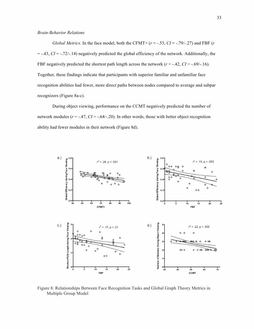
Brain-Behavior Relations
Global Metrics. In the face model, both the CFMT+ (r = -.53, CI = -.79/-.27) and FBF (r
= -.43, CI = -.72/-.14) negatively predicted the global efficiency of the network. Additionally, the
FBF negatively predicted the shortest path length across the network (r = -.42, CI = -.69/-.16).
Together, these findings indicate that participants with superior familiar and unfamiliar face
recognition abilities had fewer, more direct paths between nodes compared to average and subpar
recognizers (Figure 8a-c).
During object viewing, performance on the CCMT negatively predicted the number of
network modules (r = -.47, CI = -.64/-.20). In other words, those with better object recognition
ability had fewer modules in their network (Figure 8d).
Figure 8: Relationships Between Face Recognition Tasks and Global Graph Theory Metrics in Multiple Group Model
34
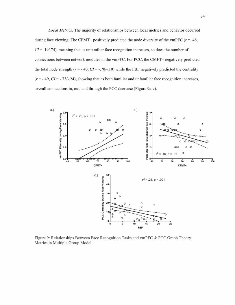
Local Metrics. The majority of relationships between local metrics and behavior occurred
during face viewing. The CFMT+ positively predicted the node diversity of the vmPFC (r = .46,
CI = .19/.74), meaning that as unfamiliar face recognition increases, so does the number of
connections between network modules in the vmPFC. For PCC, the CMFT+ negatively predicted
the total node strength (r = -.40, CI = -.70/-.10) while the FBF negatively predicted the centrality
(r = -.49, CI = -.73/-.24), showing that as both familiar and unfamiliar face recognition increases,
overall connections in, out, and through the PCC decrease (Figure 9a-c).
Figure 9: Relationships Between Face Recognition Tasks and vmPFC & PCC Graph Theory Metrics in Multiple Group Model

35
In the right amygdala, the CFMT+ negatively predicted the total node strength (r = -.41,
CI = -.73/-.09), while the CCMT negatively predicted centrality (r = -.46, CI = -.71/-.22). This
means that as both unfamiliar face and object recognition increases, overall connections in, out,
and through the right amygdala decrease (Figure 10a,b). For the left amygdala, both CFMT+ (r =
-.39, CI = -.67/-.11) and FBF (r = -.41, CI = -.71/-.11) negatively predicted clustering. The FBF
also negatively predicted centrality in the left amygdala (r = -.51, CI = -.74/-.28). In other words,
as both familiar and unfamiliar face recognition increases, the left amygdala becomes more
isolated from other regions in the face processing network (Figure 10c-e).
Finally, during object viewing, the FBF positively predicted the total connection strength
of the right pSTS (r = .43, CI = .15/.71), meaning that as familiar face recognition increases, so
does the number of connections into and out of the right pSTS (Figure 11a). In contrast to the
face model, the CCMT positively predicted the node diversity of the vmPFC (r = -.42, CI = -.74/-
.10). This shows that as object recognition ability increases, so does the number of intermodular
connections in the vmPFC (Figure 11b).
Taken together, this pattern of findings shows that as recognition ability increases,
especially for faces, more limbic and posterior face processing regions act less like hubs and
become less integral while the most anterior face regions, primarily the vmPFC, increases in
network participation and hub-like activity.

36
Figure 10: Relationships Between Face Recognition Tasks and Amygdale Graph Theory Metrics in Multiple Group Model

37
Figure 11: Relationships Between Face Recognition Tasks and Graph Theory Metrics in Multiple Group Model

38
Pattern Recognition
As stated previously, a central goal of this project is to understand whether the overall
pattern of directional connections among the nodes of the network varies between groups. As
with the previous analyses, I evaluated whether patterns of connections generated only for the
multiple group models (see Table 56).
Within-Group Comparison
For high performers, paired samples t-test show connectivity networks differed when
viewing objects versus faces (t(11) = 3.65, p < .005), but not faces versus places (t(11) = 2.14, p =
n.s) or objects versus places (t(11) = 0.40, p = n.s.). This means that for high performers, the
patterns of connectivity for individual participants are more similar to each other when viewing
faces than when viewing objects; however, they are also equally similar when viewing places.
For average performers, paired samples t-test show connectivity networks did not differ when
viewing objects versus faces (t(15) = 1.33, p = n.s.), faces versus places (t(15) = 1.64, p = n.s.), or
objects versus places (t(15) = 1.11, p = n.s.).For low performers, paired samples t-test show
connectivity networks did not differ when viewing objects versus faces (t(11) = 0.30, p = n.s.),
faces versus places (t(11) = 0.96, p = n.s.), or objects versus places (t(11) = 1.28, p = n.s.).
In sum, only high face recognizers show a distinct difference in the pattern of
connections when viewing faces compared to objects. Neither average nor low recognizers have
distinct patterns of connections during any viewing condition.
Between-Group Comparison
Given the difference between object and face organization in the face network for high
performers, I then tested whether performance groups varied more around their group pattern or a
different group pattern (e.g. do high performers vary similarly around their mean compared to the
low group mean during face viewing; see Table 5).
When viewing faces, high performers varied more from the average (t(11) = 7.98, p <
.001) and low (t(11) = 15.13 p < .001) group means compared to their own mean, but varied

39
equally from the average compared to the low means (t(11) = 2.81, p = n.s.). This indicates that
individual high recognizers have more similar patterns of connections to each other than to
individuals in the average or low group when viewing faces.
For average performers, they also varied more from the the high (t(15) = 8.03, p < .001)
and low (t(15) = 10.18, p < .001) group means compared to their own mean. This indicates that
individual average performers have more similar patterns of connections to each other than to
individuals in the high or low group when viewing faces. Additionally, average performers varied
more from the low group mean compared to the high group mean (t(15) = 9.78, p < .001). This
indicates that individual average performers have more similar patterns of connections to the high
group than to the low group when viewing faces.
Finally, low performers varied equally around the high (t(11) = 1.16, p = n.s.) and
average (t(11) = 1.74, p = n.s.) group means compared to their own group mean, indicating that
unlike the average and high recognizers, low recognizers do not have a consistent pattern of
connections among themselves.
Taken together, these results show that high performers form a unique pattern of
connections in the face-processing network when viewing faces that is distinct from that of both
average and low performers. Although individuals in the average performer group also exhibit a
unique pattern of connections during face viewing, compared to the other groups, this pattern is
not specific to face viewing; it is common across all viewing conditions. Only the high
performers exhibit modulation in their patterns of connections across viewing conditions.

40
Table 4: Relationship Between Behavioral Measures and Global Graph Theory Metrics in Single Group Model
CFMT FBF CCMT
Category Metric F r2 p F r2 p F r2 p
All Faces Shortest Path Length 2.69 0.07 n.s. 0.01 0.00 n.s. 0.16 0.00 n.s. Global Efficiency 5.37 0.12 n.s. 0.00 0.00 n.s. 1.03 0.03 n.s.
Clustering Coefficient 2.53 0.06 n.s. 5.15 0.12 n.s. 1.20 0.03 n.s.
Centrality 2.12 0.05 n.s. 0.02 0.00 n.s. 0.05 0.00 n.s. Network Density 5.46 0.13 n.s. 0.52 0.01 n.s. 0.40 0.01 n.s.
Modularity 0.01 0.00 n.s. 1.64 0.04 n.s. 0.56 0.01 n.s.
Objects Shortest Path Length 0.04 0.00 n.s. 1.62 0.04 n.s. 1.84 0.05 n.s. Global Efficiency 1.91 0.05 n.s. 0.00 0.00 n.s. 0.41 0.01 n.s.
Clustering Coefficient 1.75 0.04 n.s. 0.00 0.00 n.s. 1.76 0.04 n.s.
Centrality 0.01 0.00 n.s. 2.20 0.05 n.s. 1.91 0.05 n.s. Network Density 1.78 0.04 n.s. 0.43 0.01 n.s. 0.04 0.00 n.s.
Modularity 0.30 0.01 n.s. 0.44 0.01 n.s. 0.55 0.01 n.s.
Places Shortest Path Length 0.02 0.00 n.s. 0.52 0.01 n.s. 0.07 0.00 n.s. Global Efficiency 0.00 0.00 n.s. 1.75 0.04 n.s. 0.00 0.00 n.s.
Clustering Coefficient 0.00 0.00 n.s. 0.23 0.01 n.s. 2.01 0.05 n.s.
Centrality 0.04 0.00 n.s. 0.28 0.01 n.s. 0.10 0.00 n.s. Network Density 0.09 0.00 n.s. 1.30 0.03 n.s. 0.37 0.01 n.s.
Modularity 1.19 0.03 n.s. 3.50 0.08 n.s. 0.33 0.01 n.s.

41
Table 5: Relationship Between Behavioral Measures and Centrality in Single Group Model for Face Viewing
CFMT FBF CCMT
Category ROI F r2 p F r2 p F r2 p
Core Regions rFFA 0.07 0.00 n.s. 3.09 0.08 n.s. 1.99 0.05 n.s. lFFA 0.01 0.00 n.s. 0.00 0.00 n.s. 0.02 0.00 n.s. rOFA 1.45 0.04 n.s. 5.17 0.12 n.s. 0.04 0.00 n.s. rpSTS 2.05 0.05 n.s. 1.31 0.03 n.s. 0.86 0.02 n.s. lpSTS 2.79 0.07 n.s. 1.55 0.04 n.s. 0.56 0.01 n.s.
Extended Regions
vmPFC 0.05 0.00 n.s. 0.00 0.00 n.s. 0.52 0.01 n.s. PCC 2.25 0.06 n.s. 1.53 0.04 n.s. 0.64 0.02 n.s. rAmyg 0.74 0.02 n.s. 0.10 0.00 n.s. 1.89 0.05 n.s. lAmyg 1.91 0.05 n.s. 0.81 0.02 n.s. 0.70 0.02 n.s.
rCaudate 0.33 0.01 n.s. 0.05 0.00 n.s. 0.11 0.00 n.s.
lCaudate 0.20 0.01 n.s. 0.18 0.00 n.s. 4.44 0.10 n.s.

42
Table 6: Relationship Between Behavioral Measures and Centrality in Single Group Model for Object Viewing
CFMT FBF CCMT
Category ROI F r2 p F r2 p F r2 p
Core Regions rFFA 0.25 0.01 n.s. 1.50 0.04 n.s. 1.67 0.04 n.s. lFFA 0.81 0.02 n.s. 3.13 0.08 n.s. 0.08 0.00 n.s. rOFA 0.04 0.00 n.s. 1.47 0.04 n.s. 0.00 0.00 n.s. rpSTS 0.90 0.02 n.s. 6.11 0.14 n.s. 2.65 0.07 n.s. lpSTS 0.45 0.01 n.s. 0.13 0.00 n.s. 1.98 0.05 n.s.
Extended Regions
vmPFC 0.64 0.02 n.s. 0.40 0.01 n.s. 1.28 0.03 n.s. PCC 0.44 0.01 n.s. 1.02 0.03 n.s. 0.17 0.00 n.s. rAmyg 0.08 0.00 n.s. 0.82 0.02 n.s. 2.77 0.07 n.s. lAmyg 2.94 0.07 n.s. 1.30 0.03 n.s. 0.28 0.01 n.s.
rCaudate 0.01 0.00 n.s. 2.69 0.07 n.s. 0.67 0.02 n.s.
lCaudate 0.30 0.01 n.s. 0.69 0.02 n.s. 1.25 0.03 n.s.

43
Table 7: Relationship Between Behavioral Measures and Centrality in Single Group Model for Place Viewing
CFMT FBF CCMT
Category ROI F r2 p F r2 p F r2 p
Core Regions rFFA 5.04 0.12 n.s. 0.11 0.00 n.s. 0.12 0.00 n.s. lFFA 0.26 0.01 n.s. 0.32 0.01 n.s. 0.53 0.01 n.s. rOFA 0.20 0.01 n.s. 0.49 0.01 n.s. 0.23 0.01 n.s. rpSTS 0.63 0.02 n.s. 0.57 0.01 n.s. 0.24 0.01 n.s. lpSTS 1.55 0.04 n.s. 0.01 0.00 n.s. 0.07 0.00 n.s.
Extended Regions
vmPFC 0.41 0.01 n.s. 0.00 0.00 n.s. 0.55 0.01 n.s. PCC 1.50 0.04 n.s. 4.26 0.10 n.s. 0.96 0.02 n.s. rAmyg 1.74 0.04 n.s. 0.25 0.01 n.s. 0.41 0.01 n.s. lAmyg 0.08 0.00 n.s. 0.07 0.00 n.s. 0.05 0.00 n.s.
rCaudate 0.61 0.02 n.s. 0.05 0.00 n.s. 0.14 0.00 n.s.
lCaudate 0.64 0.02 n.s. 0.14 0.00 n.s. 0.76 0.02 n.s.

44
Table 8: Relationship Between Behavioral Measures and Clustering Coefficient in Single Group Model for Face Viewing
CFMT FBF CCMT
Category ROI F r2 p F r2 p F r2 p
Core Regions rFFA 4.24 0.10 n.s. 12.08 0.24 0.001 1.76 0.04 n.s. lFFA 2.12 0.05 n.s. 2.67 0.07 n.s. 0.00 0.00 n.s. rOFA 0.70 0.02 n.s. 1.66 0.04 n.s. 5.81 0.13 n.s. rpSTS 0.00 0.00 n.s. 1.12 0.03 n.s. 0.06 0.00 n.s. lpSTS 2.30 0.06 n.s. 0.31 0.01 n.s. 1.86 0.05 n.s.
Extended Regions
vmPFC 0.56 0.01 n.s. 0.96 0.02 n.s. 1.16 0.03 n.s. PCC 0.54 0.01 n.s. 0.56 0.01 n.s. 1.21 0.03 n.s. rAmyg 3.56 0.09 n.s. 2.54 0.06 n.s. 0.39 0.01 n.s. lAmyg 0.98 0.03 n.s. 4.31 0.10 n.s. 0.14 0.00 n.s.
rCaudate 0.00 0.00 n.s. 0.86 0.02 n.s. 0.25 0.01 n.s.
lCaudate 0.17 0.00 n.s. 0.15 0.00 n.s. 0.17 0.00 n.s.

45
Table 9: Relationship Between Behavioral Measures and Clustering Coefficient in Single Group Model for Object Viewing
CFMT FBF CCMT
Category ROI F r2 p F r2 p F r2 p
Core Regions rFFA 6.96 0.15 0.01 5.53 0.13 n.s. 0.25 0.01 n.s. lFFA 1.32 0.03 n.s. 0.00 0.00 n.s. 1.19 0.03 n.s. rOFA 0.21 0.01 n.s. 2.99 0.07 n.s. 3.51 0.08 n.s. rpSTS 4.50 0.11 n.s. 0.71 0.02 n.s. 1.68 0.04 n.s. lpSTS 7.08 0.16 0.01 0.01 0.00 n.s. 1.79 0.05 n.s.
Extended Regions
vmPFC 4.54 0.11 n.s. 0.12 0.00 n.s. 0.59 0.02 n.s. PCC 3.89 0.09 n.s. 1.62 0.04 n.s. 0.04 0.00 n.s. rAmyg 0.17 0.00 n.s. 1.30 0.03 n.s. 0.27 0.01 n.s. lAmyg 0.41 0.01 n.s. 0.24 0.01 n.s. 0.01 0.00 n.s.
rCaudate 0.23 0.01 n.s. 0.30 0.01 n.s. 1.03 0.03 n.s.
lCaudate 0.56 0.01 n.s. 0.00 0.00 n.s. 0.51 0.01 n.s.

46
Table 10: Relationship Between Behavioral Measures and Clustering Coefficient in Single Group Model for Place Viewing
CFMT FBF CCMT
Category ROI F r2 p F r2 p F r2 p
Core Regions rFFA 0.06 0.00 n.s. 1.24 0.03 n.s. 0.88 0.02 n.s. lFFA 0.04 0.00 n.s. 0.77 0.02 n.s. 0.55 0.01 n.s. rOFA 2.40 0.06 n.s. 0.95 0.02 n.s. 1.99 0.05 n.s. rpSTS 0.10 0.00 n.s. 0.01 0.00 n.s. 0.04 0.00 n.s. lpSTS 1.49 0.04 n.s. 0.01 0.00 n.s. 0.10 0.00 n.s.
Extended Regions
vmPFC 0.57 0.01 n.s. 3.16 0.08 n.s. 0.79 0.02 n.s. PCC 1.26 0.03 n.s. 0.18 0.00 n.s. 3.95 0.09 n.s. rAmyg 0.02 0.00 n.s. 0.48 0.01 n.s. 0.89 0.02 n.s. lAmyg 0.82 0.02 n.s. 0.03 0.00 n.s. 6.13 0.14 n.s.
rCaudate 0.80 0.02 n.s. 0.14 0.00 n.s. 1.62 0.04 n.s.
lCaudate 0.41 0.01 n.s. 0.54 0.01 n.s. 0.15 0.00 n.s.

47
Table 11: Relationship Between Behavioral Measures and Diversity in Single Group Model for Face Viewing
CFMT FBF CCMT
Category ROI F r2 p F r2 p F r2 p
Core Regions rFFA 1.32 0.03 n.s. 5.91 0.13 n.s. 0.76 0.02 n.s. lFFA 2.25 0.06 n.s. 0.00 0.00 n.s. 0.68 0.02 n.s. rOFA 0.21 0.01 n.s. 0.64 0.02 n.s. 0.00 0.00 n.s. rpSTS 3.11 0.08 n.s. 1.68 0.04 n.s. 0.18 0.00 n.s. lpSTS 0.01 0.00 n.s. 0.69 0.02 n.s. 0.62 0.02 n.s.
Extended Regions
vmPFC 0.41 0.01 n.s. 0.01 0.00 n.s. 0.05 0.00 n.s. PCC 0.59 0.02 n.s. 0.01 0.00 n.s. 0.01 0.00 n.s. rAmyg 0.10 0.00 n.s. 0.37 0.01 n.s. 0.00 0.00 n.s. lAmyg 2.26 0.06 n.s. 2.45 0.06 n.s. 0.47 0.01 n.s.
rCaudate 0.11 0.00 n.s. 1.05 0.03 n.s. 1.13 0.03 n.s.
lCaudate 0.61 0.02 n.s. 0.37 0.01 n.s. 0.09 0.00 n.s.

48
Table 12: Relationship Between Behavioral Measures and Diversity in Single Group Model for Object Viewing
CFMT FBF CCMT
Category ROI F r2 p F r2 p F r2 p
Core Regions rFFA 0.00 0.00 n.s. 0.05 0.00 n.s. 0.24 0.01 n.s. lFFA 0.59 0.02 n.s. 0.12 0.00 n.s. 2.05 0.05 n.s. rOFA 0.04 0.00 n.s. 0.04 0.00 n.s. 3.74 0.09 n.s. rpSTS 2.16 0.05 n.s. 0.06 0.00 n.s. 0.17 0.00 n.s. lpSTS 0.12 0.00 n.s. 0.07 0.00 n.s. 0.66 0.02 n.s.
Extended Regions
vmPFC 0.02 0.00 n.s. 0.08 0.00 n.s. 0.01 0.00 n.s. PCC 0.01 0.00 n.s. 0.86 0.02 n.s. 0.89 0.02 n.s. rAmyg 0.95 0.02 n.s. 0.53 0.01 n.s. 2.52 0.06 n.s. lAmyg 0.04 0.00 n.s. 0.53 0.01 n.s. 0.06 0.00 n.s.
rCaudate 0.05 0.00 n.s. 0.20 0.01 n.s. 0.01 0.00 n.s.
lCaudate 0.40 0.01 n.s. 0.01 0.00 n.s. 2.69 0.07 n.s.

49
Table 13: Relationship Between Behavioral Measures and Diversity in Single Group Model for Place Viewing
CFMT FBF CCMT
Category ROI F r2 p F r2 p F r2 p
Core Regions rFFA 0.09 0.00 n.s. 0.08 0.00 n.s. 0.15 0.00 n.s. lFFA 0.15 0.00 n.s. 0.00 0.00 n.s. 0.90 0.02 n.s. rOFA 0.15 0.00 n.s. 0.06 0.00 n.s. 1.81 0.05 n.s. rpSTS 2.35 0.06 n.s. 0.72 0.02 n.s. 0.01 0.00 n.s. lpSTS 0.00 0.00 n.s. 0.33 0.01 n.s. 1.47 0.04 n.s.
Extended Regions
vmPFC 0.85 0.02 n.s. 0.01 0.00 n.s. 3.44 0.08 n.s. PCC 0.19 0.01 n.s. 0.12 0.00 n.s. 0.44 0.01 n.s. rAmyg 0.05 0.00 n.s. 0.39 0.01 n.s. 0.04 0.00 n.s. lAmyg 2.13 0.05 n.s. 3.95 0.09 n.s. 2.85 0.07 n.s.
rCaudate 0.82 0.02 n.s. 2.10 0.05 n.s. 0.00 0.00 n.s.
lCaudate 2.40 0.06 n.s. 0.18 0.00 n.s. 0.05 0.00 n.s.

50
Table 14: Relationship Between Behavioral Measures and Connection Strength Total in Single Group Model for Face Viewing
CFMT FBF CCMT
Category ROI F r2 p F r2 p F r2 p
Core Regions rFFA 0.82 0.02 n.s. 0.01 0.00 n.s. 0.58 0.01 n.s. lFFA 0.01 0.00 n.s. 0.00 0.00 n.s. 3.04 0.07 n.s. rOFA 2.31 0.06 n.s. 2.59 0.06 n.s. 2.09 0.05 n.s. rpSTS 8.87 0.19 0.005 2.60 0.06 n.s. 3.47 0.08 n.s. lpSTS 6.80 0.15 n.s. 2.55 0.06 n.s. 0.74 0.02 n.s.
Extended Regions
vmPFC 0.14 0.00 n.s. 0.33 0.01 n.s. 0.14 0.00 n.s. PCC 2.08 0.05 n.s. 1.88 0.05 n.s. 1.17 0.03 n.s. rAmyg 3.62 0.09 n.s. 1.74 0.04 n.s. 0.22 0.01 n.s. lAmyg 4.83 0.11 n.s. 4.14 0.10 n.s. 1.13 0.03 n.s.
rCaudate 0.01 0.00 n.s. 0.39 0.01 n.s. 0.00 0.00 n.s.
lCaudate 0.10 0.00 n.s. 2.44 0.06 n.s. 1.15 0.03 n.s.

51
Table 15: Relationship Between Behavioral Measures and Connection Strength Total in Single Group Model for Object Viewing
CFMT FBF CCMT
Category ROI F r2 p F r2 p F r2 p
Core Regions rFFA 0.12 0.00 n.s. 0.92 0.02 n.s. 0.46 0.01 n.s. lFFA 0.51 0.01 n.s. 0.00 0.00 n.s. 1.34 0.03 n.s. rOFA 4.21 0.10 n.s. 0.90 0.02 n.s. 0.11 0.00 n.s. rpSTS 0.33 0.01 n.s. 1.23 0.03 n.s. 1.00 0.03 n.s. lpSTS 1.60 0.04 n.s. 1.86 0.05 n.s. 0.11 0.00 n.s.
Extended Regions
vmPFC 0.94 0.02 n.s. 0.17 0.00 n.s. 0.02 0.00 n.s. PCC 2.95 0.07 n.s. 3.17 0.08 n.s. 0.93 0.02 n.s. rAmyg 0.00 0.00 n.s. 0.06 0.00 n.s. 2.09 0.05 n.s. lAmyg 1.88 0.05 n.s. 4.60 0.11 n.s. 1.53 0.04 n.s.
rCaudate 0.00 0.00 n.s. 0.68 0.02 n.s. 0.45 0.01 n.s.
lCaudate 0.27 0.01 n.s. 0.41 0.01 n.s. 0.87 0.02 n.s.

52
Table 16: Relationship Between Behavioral Measures and Connection Strength Total in Single Group Model for Place Viewing
CFMT FBF CCMT
Category ROI F r2 p F r2 p F r2 p
Core Regions rFFA 0.30 0.01 n.s. 1.49 0.04 n.s. 0.02 0.00 n.s. lFFA 0.03 0.00 n.s. 0.09 0.00 n.s. 0.06 0.00 n.s. rOFA 0.04 0.00 n.s. 0.51 0.01 n.s. 0.24 0.01 n.s. rpSTS 1.92 0.05 n.s. 0.17 0.00 n.s. 0.05 0.00 n.s. lpSTS 0.64 0.02 n.s. 0.22 0.01 n.s. 0.04 0.00 n.s.
Extended Regions
vmPFC 0.51 0.01 n.s. 2.51 0.06 n.s. 3.39 0.08 n.s. PCC 0.00 0.00 n.s. 1.06 0.03 n.s. 0.99 0.03 n.s. rAmyg 0.00 0.00 n.s. 0.29 0.01 n.s. 0.87 0.02 n.s. lAmyg 0.88 0.02 n.s. 0.57 0.01 n.s. 0.95 0.02 n.s.
rCaudate 1.15 0.03 n.s. 0.36 0.01 n.s. 0.00 0.00 n.s.
lCaudate 0.03 0.00 n.s. 0.73 0.02 n.s. 0.07 0.00 n.s.

53
Table 17: Relationship Between Behavioral Measures and Global Graph Theory Metrics in Individual Model
CFMT FBF CCMT
Category Metric F df p F df p F df p
All Faces Shortest Path Length 1.28 0.03 n.s. 0.02 0.00 n.s. 0.00 0.00 n.s. Global Efficiency 0.91 0.02 n.s. 0.00 0.00 n.s. 0.75 0.02 n.s.
Clustering Coefficient 2.29 0.06 n.s. 0.70 0.02 n.s. 1.75 0.04 n.s.
Centrality 1.36 0.03 n.s. 0.03 0.00 n.s. 0.01 0.00 n.s. Network Density 0.93 0.02 n.s. 0.03 0.00 n.s. 2.82 0.07 n.s.
Modularity 0.32 0.01 n.s. 0.19 0.01 n.s. 0.41 0.01 n.s.
Objects Shortest Path Length 0.01 0.00 n.s. 0.24 0.01 n.s. 2.61 0.06 n.s. Global Efficiency 0.01 0.00 n.s. 0.01 0.00 n.s. 1.80 0.05 n.s.
Clustering Coefficient 0.00 0.00 n.s. 0.29 0.01 n.s. 1.72 0.04 n.s.
Centrality 0.02 0.00 n.s. 0.31 0.01 n.s. 2.52 0.06 n.s. Network Density 0.05 0.00 n.s. 0.09 0.00 n.s. 0.34 0.01 n.s.
Modularity 2.36 0.06 n.s. 3.82 0.09 n.s. 0.00 0.00 n.s.
Places Shortest Path Length 0.00 0.00 n.s. 0.56 0.01 n.s. 0.68 0.02 n.s. Global Efficiency 0.06 0.00 n.s. 0.76 0.02 n.s. 0.43 0.01 n.s.
Clustering Coefficient 1.71 0.04 n.s. 3.64 0.09 n.s. 1.81 0.05 n.s.
Centrality 0.01 0.00 n.s. 0.52 0.01 n.s. 0.65 0.02 n.s. Network Density 0.00 0.00 n.s. 1.12 0.03 n.s. 0.17 0.00 n.s.
Modularity 4.42 0.10 n.s. 1.12 0.03 n.s. 2.72 0.07 n.s.

54
Table 18: Relationship Between Behavioral Measures and Centrality in Individual Model for Face Viewing
CFMT FBF CCMT
Category ROI F r2 p F r2 p F r2 p
Core Regions rFFA 0.95 0.02 n.s. 0.35 0.01 n.s. 0.18 0.00 n.s. lFFA 0.06 0.00 n.s. 1.12 0.03 n.s. 7.08 0.16 0.01 rOFA 2.11 0.05 n.s. 2.20 0.05 n.s. 0.89 0.02 n.s. rpSTS 0.14 0.00 n.s. 0.13 0.00 n.s. 0.35 0.01 n.s. lpSTS 5.33 0.12 n.s. 1.88 0.05 n.s. 4.20 0.10 n.s.
Extended Regions
vmPFC 0.10 0.00 n.s. 1.56 0.04 n.s. 0.59 0.02 n.s. PCC 0.08 0.00 n.s. 0.82 0.02 n.s. 0.02 0.00 n.s. rAmyg 3.24 0.08 n.s. 1.38 0.03 n.s. 3.35 0.08 n.s. lAmyg 2.52 0.06 n.s. 1.74 0.04 n.s. 0.02 0.00 n.s.
rCaudate 0.47 0.01 n.s. 0.02 0.00 n.s. 1.91 0.05 n.s.
lCaudate 1.00 0.03 n.s. 0.47 0.01 n.s. 1.60 0.04 n.s.

55
Table 18: Relationship Between Behavioral Measures and Centrality in Individual Model for Object Viewing
CFMT FBF CCMT
Category ROI F r2 p F r2 p F r2 p
Core Regions rFFA 0.11 0.00 n.s. 0.09 0.00 n.s. 5.83 0.13 n.s. lFFA 0.06 0.00 n.s. 0.02 0.00 n.s. 0.04 0.00 n.s. rOFA 0.73 0.02 n.s. 1.77 0.04 n.s. 0.31 0.01 n.s. rpSTS 0.13 0.00 n.s. 0.39 0.01 n.s. 1.85 0.05 n.s. lpSTS 0.07 0.00 n.s. 0.45 0.01 n.s. 0.31 0.01 n.s.
Extended Regions
vmPFC 2.89 0.07 n.s. 1.77 0.04 n.s. 1.12 0.03 n.s. PCC 0.20 0.01 n.s. 0.17 0.00 n.s. 0.00 0.00 n.s. rAmyg 0.82 0.02 n.s. 0.72 0.02 n.s. 0.10 0.00 n.s. lAmyg 0.02 0.00 n.s. 2.77 0.07 n.s. 1.97 0.05 n.s.
rCaudate 0.64 0.02 n.s. 1.19 0.03 n.s. 0.07 0.00 n.s.
lCaudate 0.00 0.00 n.s. 0.03 0.00 n.s. 0.29 0.01 n.s.

56
Table 20: Relationship Between Behavioral Measures and Centrality in Individual Model for Place Viewing
CFMT FBF CCMT
Category ROI F r2 p F r2 p F r2 p
Core Regions rFFA 0.02 0.00 n.s. 2.93 0.07 n.s. 0.09 0.00 n.s. lFFA 1.73 0.04 n.s. 0.06 0.00 n.s. 0.84 0.02 n.s. rOFA 1.62 0.04 n.s. 0.76 0.02 n.s. 1.29 0.03 n.s. rpSTS 0.00 0.00 n.s. 0.01 0.00 n.s. 8.47 0.18 0.01 lpSTS 0.39 0.01 n.s. 1.81 0.05 n.s. 0.71 0.02 n.s.
Extended Regions
vmPFC 0.14 0.00 n.s. 0.06 0.00 n.s. 0.03 0.00 n.s. PCC 0.01 0.00 n.s. 0.00 0.00 n.s. 0.63 0.02 n.s. rAmyg 0.02 0.00 n.s. 0.00 0.00 n.s. 0.06 0.00 n.s. lAmyg 0.42 0.01 n.s. 0.93 0.02 n.s. 0.54 0.01 n.s.
rCaudate 3.40 0.08 n.s. 1.16 0.03 n.s. 0.76 0.02 n.s.
lCaudate 0.08 0.00 n.s. 0.73 0.02 n.s. 1.00 0.03 n.s.

57
Table 21: Relationship Between Behavioral Measures and Clustering Coefficient in Individual Model for Face Viewing
CFMT FBF CCMT
Category ROI F r2 p F r2 p F r2 p
Core Regions rFFA 1.55 0.04 n.s. 1.03 0.03 n.s. 0.36 0.01 n.s. lFFA 1.81 0.05 n.s. 0.56 0.01 n.s. 0.54 0.01 n.s. rOFA 0.02 0.00 n.s. 0.03 0.00 n.s. 2.91 0.07 n.s. rpSTS 0.44 0.01 n.s. 0.06 0.00 n.s. 1.54 0.04 n.s. lpSTS 1.66 0.04 n.s. 0.23 0.01 n.s. 4.79 0.11 n.s.
Extended Regions
vmPFC 0.01 0.00 n.s. 3.29 0.08 n.s. 0.11 0.00 n.s. PCC 0.09 0.00 n.s. 1.22 0.03 n.s. 0.28 0.01 n.s. rAmyg 0.02 0.00 n.s. 0.02 0.00 n.s. 1.89 0.05 n.s. lAmyg 0.15 0.00 n.s. 0.42 0.01 n.s. 2.06 0.05 n.s.
rCaudate 3.56 0.09 n.s. 0.48 0.01 n.s. 0.71 0.02 n.s.
lCaudate 4.72 0.11 n.s. 2.36 0.06 n.s. 0.15 0.00 n.s.

58
Table 22: Relationship Between Behavioral Measures and Clustering Coefficient in Individual Model for Object Viewing
CFMT FBF CCMT
Category ROI F r2 p F r2 p F r2 p
Core Regions rFFA 0.14 0.00 n.s. 0.45 0.01 n.s. 1.81 0.05 n.s. lFFA 0.01 0.00 n.s. 0.03 0.00 n.s. 0.28 0.01 n.s. rOFA 0.05 0.00 n.s. 0.02 0.00 n.s. 1.66 0.04 n.s. rpSTS 0.67 0.02 n.s. 0.33 0.01 n.s. 0.01 0.00 n.s. lpSTS 4.62 0.11 n.s. 1.89 0.05 n.s. 0.02 0.00 n.s.
Extended Regions
vmPFC 0.11 0.00 n.s. 0.02 0.00 n.s. 0.06 0.00 n.s. PCC 0.51 0.01 n.s. 0.82 0.02 n.s. 1.38 0.04 n.s. rAmyg 0.15 0.00 n.s. 0.36 0.01 n.s. 2.87 0.07 n.s. lAmyg 0.24 0.01 n.s. 0.14 0.00 n.s. 0.67 0.02 n.s.
rCaudate 0.12 0.00 n.s. 0.02 0.00 n.s. 0.20 0.01 n.s.
lCaudate 1.00 0.03 n.s. 0.18 0.00 n.s. 1.10 0.03 n.s.

59
Table 23: Relationship Between Behavioral Measures and Clustering Coefficient in Individual Model for Place Viewing
CFMT FBF CCMT
Category ROI F r2 p F r2 p F r2 p
Core Regions rFFA 1.87 0.05 n.s. 6.30 0.14 n.s. 0.12 0.00 n.s. lFFA 0.55 0.01 n.s. 0.00 0.00 n.s. 2.07 0.05 n.s. rOFA 0.98 0.03 n.s. 2.06 0.05 n.s. 1.75 0.04 n.s. rpSTS 0.01 0.00 n.s. 0.76 0.02 n.s. 0.11 0.00 n.s. lpSTS 0.80 0.02 n.s. 0.17 0.00 n.s. 5.09 0.12 n.s.
Extended Regions
vmPFC 0.33 0.01 n.s. 2.41 0.06 n.s. 0.02 0.00 n.s. PCC 0.63 0.02 n.s. 0.66 0.02 n.s. 3.50 0.08 n.s. rAmyg 0.97 0.02 n.s. 1.64 0.04 n.s. 1.42 0.04 n.s. lAmyg 0.40 0.01 n.s. 0.20 0.01 n.s. 0.90 0.02 n.s.
rCaudate 0.04 0.00 n.s. 0.44 0.01 n.s. 0.78 0.02 n.s.
lCaudate 0.00 0.00 n.s. 0.02 0.00 n.s. 0.02 0.00 n.s.

60
Table 24: Relationship Between Behavioral Measures and Diversity in Individual Model for Face Viewing
CFMT FBF CCMT
Category ROI F r2 p F r2 p F r2 p
Core Regions rFFA 0.82 0.02 n.s. 0.42 0.01 n.s. 0.16 0.00 n.s. lFFA 2.37 0.06 n.s. 0.73 0.02 n.s. 1.28 0.03 n.s. rOFA 0.47 0.01 n.s. 0.01 0.00 n.s. 0.07 0.00 n.s. rpSTS 8.99 0.19 0.005 10.83 0.22 0.002 0.76 0.02 n.s. lpSTS 1.78 0.04 n.s. 0.80 0.02 n.s. 3.85 0.09 n.s.
Extended Regions
vmPFC 3.12 0.08 n.s. 2.41 0.06 n.s. 0.03 0.00 n.s. PCC 0.00 0.00 n.s. 0.07 0.00 n.s. 0.14 0.00 n.s. rAmyg 1.82 0.05 n.s. 5.43 0.13 n.s. 3.18 0.08 n.s. lAmyg 0.00 0.00 n.s. 0.00 0.00 n.s. 0.61 0.02 n.s.
rCaudate 7.48 0.16 0.01 1.98 0.05 n.s. 4.45 0.10 n.s.
lCaudate 0.73 0.02 n.s. 0.19 0.00 n.s. 2.65 0.07 n.s.

61
Table 25: Relationship Between Behavioral Measures and Diversity in Individual Model for Object Viewing
CFMT FBF CCMT
Category ROI F r2 p F r2 p F r2 p
Core Regions rFFA 1.67 0.04 n.s. 0.17 0.00 n.s. 0.32 0.01 n.s. lFFA 0.88 0.02 n.s. 0.02 0.00 n.s. 0.03 0.00 n.s. rOFA 0.46 0.01 n.s. 0.45 0.01 n.s. 2.83 0.07 n.s. rpSTS 2.18 0.05 n.s. 0.90 0.02 n.s. 0.00 0.00 n.s. lpSTS 0.26 0.01 n.s. 0.20 0.01 n.s. 0.08 0.00 n.s.
Extended Regions
vmPFC 0.01 0.00 n.s. 2.81 0.07 n.s. 2.73 0.07 n.s. PCC 0.10 0.00 n.s. 0.83 0.02 n.s. 0.58 0.02 n.s. rAmyg 0.31 0.01 n.s. 0.39 0.01 n.s. 0.08 0.00 n.s. lAmyg 0.66 0.02 n.s. 0.00 0.00 n.s. 0.53 0.01 n.s.
rCaudate 0.14 0.00 n.s. 1.07 0.03 n.s. 0.41 0.01 n.s.
lCaudate 0.00 0.00 n.s. 0.52 0.01 n.s. 0.02 0.00 n.s.

62
Table 26: Relationship Between Behavioral Measures and Diversity in Individual Model for Place Viewing
CFMT FBF CCMT
Category ROI F r2 p F r2 p F r2 p
Core Regions rFFA 0.34 0.01 n.s. 0.32 0.01 n.s. 1.58 0.04 n.s. lFFA 1.05 0.03 n.s. 0.55 0.01 n.s. 0.02 0.00 n.s. rOFA 0.43 0.01 n.s. 0.03 0.00 n.s. 0.28 0.01 n.s. rpSTS 0.97 0.02 n.s. 0.79 0.02 n.s. 0.92 0.02 n.s. lpSTS 1.11 0.03 n.s. 2.94 0.07 n.s. 0.91 0.02 n.s.
Extended Regions
vmPFC 2.28 0.06 n.s. 0.08 0.00 n.s. 2.15 0.05 n.s. PCC 0.53 0.01 n.s. 1.24 0.03 n.s. 0.29 0.01 n.s. rAmyg 0.37 0.01 n.s. 0.00 0.00 n.s. 2.79 0.07 n.s. lAmyg 6.12 0.14 n.s. 1.87 0.05 n.s. 5.13 0.12 n.s.
rCaudate 0.15 0.00 n.s. 0.00 0.00 n.s. 0.04 0.00 n.s.
lCaudate 0.11 0.00 n.s. 0.02 0.00 n.s. 0.30 0.01 n.s.

63
Table 27: Relationship Between Behavioral Measures and Connection Strength Total in Individual Model for Face Viewing
CFMT FBF CCMT
Category ROI F r2 p F r2 p F r2 p
Core Regions rFFA 1.26 0.03 n.s. 0.03 0.00 n.s. 1.39 0.04 n.s. lFFA 2.78 0.07 n.s. 2.47 0.06 n.s. 0.85 0.02 n.s.
rOFA 1.08 0.03 n.s. 0.99 0.03 n.s. 28.33 0.43 <.0001
rpSTS 2.07 0.05 n.s. 0.27 0.01 n.s. 0.02 0.00 n.s. lpSTS 2.49 0.06 n.s. 2.91 0.07 n.s. 5.29 0.12 n.s.
Extended Regions
vmPFC 1.10 0.03 n.s. 1.57 0.04 n.s. 0.61 0.02 n.s. PCC 0.19 0.00 n.s. 0.13 0.00 n.s. 0.17 0.00 n.s. rAmyg 4.32 0.10 n.s. 3.62 0.09 n.s. 0.67 0.02 n.s. lAmyg 0.78 0.02 n.s. 1.92 0.05 n.s. 0.97 0.03 n.s.
rCaudate 0.39 0.01 n.s. 0.88 0.02 n.s. 5.97 0.14 n.s.
lCaudate 0.09 0.00 n.s. 0.56 0.01 n.s. 0.89 0.02 n.s.

64
Table 28: Relationship Between Behavioral Measures and Connection Strength Total in Individual Model for Object Viewing
CFMT FBF CCMT
Category ROI F r2 p F r2 p F r2 p
Core Regions rFFA 0.17 0.00 n.s. 0.11 0.00 n.s. 5.46 0.13 n.s. lFFA 0.06 0.00 n.s. 0.72 0.02 n.s. 0.49 0.01 n.s. rOFA 0.12 0.00 n.s. 0.01 0.00 n.s. 0.00 0.00 n.s. rpSTS 3.60 0.09 n.s. 1.84 0.05 n.s. 0.12 0.00 n.s. lpSTS 1.03 0.03 n.s. 0.32 0.01 n.s. 0.68 0.02 n.s.
Extended Regions
vmPFC 1.25 0.03 n.s. 0.01 0.00 n.s. 0.03 0.00 n.s. PCC 1.12 0.03 n.s. 1.83 0.05 n.s. 0.23 0.01 n.s. rAmyg 1.27 0.03 n.s. 0.01 0.00 n.s. 1.28 0.03 n.s. lAmyg 0.53 0.01 n.s. 1.49 0.04 n.s. 0.16 0.00 n.s.
rCaudate 0.07 0.00 n.s. 1.25 0.03 n.s. 2.54 0.06 n.s.
lCaudate 0.02 0.00 n.s. 0.02 0.00 n.s. 0.00 0.00 n.s.

65
Table 29: Relationship Between Behavioral Measures and Connection Strength Total in Individual Model for Place Viewing
CFMT FBF CCMT
Category ROI F r2 p F r2 p F r2 p
Core Regions rFFA 0.04 0.00 n.s. 0.43 0.01 n.s. 2.52 0.06 n.s. lFFA 0.14 0.00 n.s. 0.15 0.00 n.s. 1.33 0.03 n.s. rOFA 0.04 0.00 n.s. 0.01 0.00 n.s. 0.45 0.01 n.s. rpSTS 0.01 0.00 n.s. 0.05 0.00 n.s. 0.42 0.01 n.s. lpSTS 2.55 0.06 n.s. 4.10 0.10 n.s. 0.09 0.00 n.s.
Extended Regions
vmPFC 0.45 0.01 n.s. 0.00 0.00 n.s. 0.72 0.02 n.s. PCC 0.09 0.00 n.s. 0.07 0.00 n.s. 4.56 0.11 n.s. rAmyg 1.67 0.04 n.s. 0.06 0.00 n.s. 0.29 0.01 n.s. lAmyg 0.60 0.02 n.s. 2.67 0.07 n.s. 0.78 0.02 n.s.
rCaudate 4.43 0.10 n.s. 0.95 0.02 n.s. 0.45 0.01 n.s.
lCaudate 1.90 0.05 n.s. 4.05 0.10 n.s. 0.09 0.00 n.s.

66
Table 30: ANOVA of Global Graph Theory Metrics across All Models
Separate Model Group Model Individual Model
Category Metric F df p F df p F df p
All Faces Shortest Path Length 2.88 (2,37) n.s. 0.24 (2,37
) n.s. 1.41 (2,37) n.s.
Global Efficiency 9.35 (2,37) 0.001 1.33 (2,37) n.s. 1.83 (2,37) n.s.
Clustering Coefficient 0.49 (2,37) n.s. 1.54 (2,37
) n.s. 0.52 (2,37) n.s.
Centrality 1.76 (2,37) n.s. 0.17 (2,37) n.s. 1.31 (2,37) n.s.
Network Density 3.29 (2,37) n.s. 2.05 (2,37) n.s. 2.27 (2,37) n.s.
Modularity 1.75 (2,37) n.s. 1.25 (2,37) n.s. 0.53 (2,37) n.s.
Objects
Shortest Path Length 1.19 (2,37) n.s. 1.08 (2,37) n.s. 0.14 (2,37) n.s.
Global Efficiency 5.85 (2,37) n.s. 1.19 (2,37) n.s. 0.50 (2,37) n.s.
Clustering Coefficient 0.73 (2,37) n.s. 0.50 (2,37
) n.s. 0.77 (2,37) n.s.
Centrality 1.25 (2,37) n.s. 1.17 (2,37) n.s. 0.11 (2,37) n.s.
Network Density 4.39 (2,37) n.s. 0.93 (2,37) n.s. 0.55 (2,37) n.s.
Modularity 0.96 (2,37) n.s. 0.19 (2,37) n.s. 0.53 (2,37) n.s.
Places
Shortest Path Length 0.73 (2,37) n.s. 2.52 (2,37) n.s. 0.48 (2,37) n.s.
Global Efficiency 0.91 (2,37) n.s. 2.12 (2,37) n.s. 1.47 (2,37) n.s.
Clustering Coefficient 0.27 (2,37) n.s. 1.13 (2,37
) n.s. 0.62 (2,37) n.s.
Centrality 0.53 (2,37) n.s. 2.29 (2,37) n.s. 0.41 (2,37) n.s.
Network Density 0.31 (2,37) n.s. 0.58 (2,37) n.s. 2.24 (2,37) n.s.
Modularity 0.00 (2,37) n.s. 1.66 (2,37) n.s. 3.20 (2,37) n.s.

67
Table 31: ANOVA of Node Centrality in Face Viewing
Separate Model Group Model Individual Model
Category ROI F df p F df p F df p
Core Regions rFFA 0.537 (2,37) n.s. 0.642 (2,37) n.s. 1.651 (2,37) n.s. lFFA 0.814 (2,37) n.s. 0.488 (2,37) n.s. 0.583 (2,37) n.s. rOFA 1.904 (2,37) n.s. 1.069 (2,37) n.s. 0.580 (2,37) n.s. rpSTS 1.503 (2,37) n.s. 0.645 (2,37) n.s. 0.523 (2,37) n.s. lpSTS 0.205 (2,37) n.s. 1.066 (2,37) n.s. 1.448 (2,37) n.s.
Extended Regions
vmPFC 1.209 (2,37) n.s. 1.209 (2,37) n.s. 0.004 (2,37) n.s. PCC 1.936 (2,37) n.s. 1.936 (2,37) n.s. 0.033 (2,37) n.s. rAmyg 0.631 (2,37) n.s. 0.631 (2,37) n.s. 3.943 (2,37) n.s. lAmyg 0.382 (2,37) n.s. 0.382 (2,37) n.s. 0.792 (2,37) n.s.
rCaudate 0.023 (2,37) n.s. 0.023 (2,37) n.s. 0.448 (2,37) n.s.
lCaudate 0.122 (2,37) n.s. 0.122 (2,37) n.s. 1.452 (2,37) n.s.

68
Table 32: ANOVA of Node Centrality in Object Viewing
Separate Model Group Model Individual Model
Category ROI F df p F df p F df p
Core Regions rFFA 1.082 (2,37) n.s. 0.276 (2,37) n.s. 0.044 (2,37) n.s. lFFA 0.294 (2,37) n.s. 2.821 (2,37) n.s. 0.095 (2,37) n.s. rOFA 1.273 (2,37) n.s. 2.812 (2,37) n.s. 1.072 (2,37) n.s. rpSTS 3.709 (2,37) n.s. 2.316 (2,37) n.s. 0.423 (2,37) n.s. lpSTS 0.507 (2,37) n.s. 0.863 (2,37) n.s. 0.978 (2,37) n.s.
Extended Regions
vmPFC 0.214 (2,37) n.s. 0.214 (2,37) n.s. 0.902 (2,37) n.s. PCC 0.740 (2,37) n.s. 0.740 (2,37) n.s. 0.154 (2,37) n.s. rAmyg 0.039 (2,37) n.s. 0.039 (2,37) n.s. 0.370 (2,37) n.s. lAmyg 1.407 (2,37) n.s. 1.407 (2,37) n.s. 0.178 (2,37) n.s.
rCaudate 2.664 (2,37) n.s. 2.664 (2,37) n.s. 1.672 (2,37) n.s.
lCaudate 0.593 (2,37) n.s. 0.593 (2,37) n.s. 0.019 (2,37) n.s.

69
Table 33: ANOVA of Node Centrality in Place Viewing
Separate Model Group Model Individual Model
Category ROI F df p F df p F df p
Core Regions rFFA 2.980 (2,37) n.s. 5.255 (2,37) 0.010 3.080 (2,37) n.s. lFFA 0.795 (2,37) n.s. 0.591 (2,37) n.s. 0.277 (2,37) n.s. rOFA 6.782 (2,37) 0.003 1.048 (2,37) n.s. 0.206 (2,37) n.s. rpSTS 2.610 (2,37) n.s. 0.592 (2,37) n.s. 0.019 (2,37) n.s. lpSTS 1.796 (2,37) n.s. 1.769 (2,37) n.s. 2.403 (2,37) n.s.
Extended Regions
vmPFC 1.014 (2,37) n.s. 1.014 (2,37) n.s. 0.923 (2,37) n.s. PCC 0.743 (2,37) n.s. 0.743 (2,37) n.s. 0.111 (2,37) n.s. rAmyg 0.868 (2,37) n.s. 0.868 (2,37) n.s. 0.068 (2,37) n.s. lAmyg 1.049 (2,37) n.s. 1.049 (2,37) n.s. 0.762 (2,37) n.s.
rCaudate 0.433 (2,37) n.s. 0.433 (2,37) n.s. 1.134 (2,37) n.s.
lCaudate 0.558 (2,37) n.s. 0.558 (2,37) n.s. 0.220 (2,37) n.s.

70
Table 34: ANOVA of Node Clustering Coefficient in Face Viewing
Separate Model Group Model Individual Model
Category ROI F df p F df p F df p
Core Regions rFFA 4.498 (2,37) n.s. 1.741 (2,37) n.s. 0.086 (2,37) n.s. lFFA 2.170 (2,37) n.s. 1.030 (2,37) n.s. 1.327 (2,37) n.s. rOFA 2.104 (2,37) n.s. 0.530 (2,37) n.s. 0.337 (2,37) n.s. rpSTS 1.768 (2,37) n.s. 0.072 (2,37) n.s. 0.139 (2,37) n.s. lpSTS 0.699 (2,37) n.s. 0.037 (2,37) n.s. 0.356 (2,37) n.s.
Extended Regions
vmPFC 0.021 (2,37) n.s. 0.021 (2,37) n.s. 2.479 (2,37) n.s. PCC 0.835 (2,37) n.s. 0.835 (2,37) n.s. 1.698 (2,37) n.s. rAmyg 3.091 (2,37) n.s. 3.091 (2,37) n.s. 0.333 (2,37) n.s. lAmyg 1.097 (2,37) n.s. 1.097 (2,37) n.s. 0.897 (2,37) n.s.
rCaudate 0.628 (2,37) n.s. 0.628 (2,37) n.s. 0.970 (2,37) n.s.
lCaudate 0.535 (2,37) n.s. 0.535 (2,37) n.s. 0.521 (2,37) n.s.

71
Table 35: ANOVA of Node Clustering Coefficient in Object Viewing
Separate Model Group Model Individual Model
Category ROI F df p F df p F df p
Core Regions rFFA 1.889 (2,37) n.s. 3.664 (2,37) n.s. 0.520 (2,37) n.s. lFFA 1.886 (2,37) n.s. 1.232 (2,37) n.s. 0.130 (2,37) n.s. rOFA 2.301 (2,37) n.s. 1.360 (2,37) n.s. 0.162 (2,37) n.s. rpSTS 0.036 (2,37) n.s. 2.167 (2,37) n.s. 0.486 (2,37) n.s. lpSTS 0.237 (2,37) n.s. 5.779 (2,37) 0.007 1.855 (2,37) n.s.
Extended Regions
vmPFC 1.185 (2,37) n.s. 1.185 (2,37) n.s. 1.786 (2,37) n.s. PCC 1.311 (2,37) n.s. 1.311 (2,37) n.s. 1.413 (2,37) n.s. rAmyg 0.488 (2,37) n.s. 0.488 (2,37) n.s. 0.108 (2,37) n.s. lAmyg 2.856 (2,37) n.s. 2.856 (2,37) n.s. 0.055 (2,37) n.s.
rCaudate 0.159 (2,37) n.s. 0.159 (2,37) n.s. 0.441 (2,37) n.s.
lCaudate 0.285 (2,37) n.s. 0.285 (2,37) n.s. 0.257 (2,37) n.s.

72
Table 36: ANOVA of Node Clustering Coefficient in Place Viewing
Separate Model Group Model Individual Model
Category ROI F df p F df p F df p
Core Regions rFFA 2.269 (2,37) n.s. 1.038 (2,37) n.s. 2.715 (2,37) n.s. lFFA 1.374 (2,37) n.s. 0.338 (2,37) n.s. 0.478 (2,37) n.s. rOFA 0.125 (2,37) n.s. 0.707 (2,37) n.s. 1.258 (2,37) n.s. rpSTS 0.036 (2,37) n.s. 1.138 (2,37) n.s. 1.996 (2,37) n.s. lpSTS 2.910 (2,37) n.s. 0.971 (2,37) n.s. 0.645 (2,37) n.s.
Extended Regions
vmPFC 2.637 (2,37) n.s. 2.637 (2,37) n.s. 0.315 (2,37) n.s. PCC 1.796 (2,37) n.s. 1.796 (2,37) n.s. 0.172 (2,37) n.s. rAmyg 0.034 (2,37) n.s. 0.034 (2,37) n.s. 1.074 (2,37) n.s. lAmyg 0.530 (2,37) n.s. 0.530 (2,37) n.s. 0.163 (2,37) n.s.
rCaudate 0.958 (2,37) n.s. 0.958 (2,37) n.s. 2.142 (2,37) n.s.
lCaudate 0.547 (2,37) n.s. 0.547 (2,37) n.s. 1.258 (2,37) n.s.

73
Table 37: ANOVA of Node Diversity in Face Viewing
Separate Model Group Model Individual Model
Category ROI F df p F df p F df p
Core Regions rFFA 0.076 (2,37) n.s. 4.765 (2,37) n.s. 1.488 (2,37) n.s. lFFA 0.839 (2,37) n.s. 0.179 (2,37) n.s. 0.341 (2,37) n.s. rOFA 3.235 (2,37) n.s. 1.021 (2,37) n.s. 0.113 (2,37) n.s. rpSTS 2.958 (2,37) n.s. 1.527 (2,37) n.s. 5.516 (2,37) 0.008 lpSTS 1.008 (2,37) n.s. 0.518 (2,37) n.s. 0.516 (2,37) n.s.
Extended Regions
vmPFC 0.964 (2,37) n.s. 0.964 (2,37) n.s. 1.156 (2,37) n.s. PCC 1.080 (2,37) n.s. 1.080 (2,37) n.s. 0.635 (2,37) n.s. rAmyg 0.060 (2,37) n.s. 0.060 (2,37) n.s. 1.845 (2,37) n.s. lAmyg 0.642 (2,37) n.s. 0.642 (2,37) n.s. 0.027 (2,37) n.s.
rCaudate 0.344 (2,37) n.s. 0.344 (2,37) n.s. 1.981 (2,37) n.s.
lCaudate 0.278 (2,37) n.s. 0.278 (2,37) n.s. 0.031 (2,37) n.s.

74
Table 38: ANOVA of Node Diversity in Object Viewing
Separate Model Group Model Individual Model
Category ROI F df p F df p F df p
Core Regions rFFA 0.773 (2,37) n.s. 0.522 (2,37) n.s. 1.085 (2,37) n.s. lFFA 1.239 (2,37) n.s. 0.128 (2,37) n.s. 0.396 (2,37) n.s. rOFA 1.391 (2,37) n.s. 0.314 (2,37) n.s. 0.064 (2,37) n.s. rpSTS 4.469 (2,37) n.s. 0.417 (2,37) n.s. 1.100 (2,37) n.s. lpSTS 6.684 (2,37) 0.003 1.063 (2,37) n.s. 1.666 (2,37) n.s.
Extended Regions
vmPFC 1.865 (2,37) n.s. 1.865 (2,37) n.s. 0.395 (2,37) n.s. PCC 1.768 (2,37) n.s. 1.768 (2,37) n.s. 1.645 (2,37) n.s. rAmyg 0.395 (2,37) n.s. 0.395 (2,37) n.s. 0.162 (2,37) n.s. lAmyg 0.841 (2,37) n.s. 0.841 (2,37) n.s. 0.713 (2,37) n.s.
rCaudate 0.251 (2,37) n.s. 0.251 (2,37) n.s. 0.541 (2,37) n.s.
lCaudate 2.479 (2,37) n.s. 2.479 (2,37) n.s. 0.643 (2,37) n.s.

75
Table 39: ANOVA of Node Diversity in Place Viewing
Separate Model Group Model Individual Model
Category ROI F df p F df p F df p
Core Regions rFFA 0.966 (2,37) n.s. 0.512 (2,37) n.s. 0.385 (2,37) n.s. lFFA 2.926 (2,37) n.s. 0.513 (2,37) n.s. 0.394 (2,37) n.s. rOFA 1.456 (2,37) n.s. 1.475 (2,37) n.s. 0.157 (2,37) n.s. rpSTS 0.031 (2,37) n.s. 0.166 (2,37) n.s. 0.600 (2,37) n.s. lpSTS 1.682 (2,37) n.s. 1.557 (2,37) n.s. 5.341 (2,37) 0.009
Extended Regions
vmPFC 0.438 (2,37) n.s. 0.438 (2,37) n.s. 0.088 (2,37) n.s. PCC 0.793 (2,37) n.s. 0.793 (2,37) n.s. 1.216 (2,37) n.s. rAmyg 0.258 (2,37) n.s. 0.258 (2,37) n.s. 0.616 (2,37) n.s. lAmyg 2.086 (2,37) n.s. 2.086 (2,37) n.s. 3.681 (2,37) n.s.
rCaudate 0.705 (2,37) n.s. 0.705 (2,37) n.s. 0.329 (2,37) n.s.
lCaudate 2.020 (2,37) n.s. 2.020 (2,37) n.s. 0.774 (2,37) n.s.

76
Table 40: ANOVA of Node Total Connection Strength in Face Viewing
Separate Model Group Model Individual Model
Category ROI F df p F df p F df p
Core Regions rFFA 1.195 (2,37) n.s. 2.027 (2,37) n.s. 3.624 (2,37) n.s. lFFA 2.026 (2,37) n.s. 0.067 (2,37) n.s. 1.456 (2,37) n.s. rOFA 1.900 (2,37) n.s. 1.677 (2,37) n.s. 0.548 (2,37) n.s. rpSTS 5.275 (2,37) 0.010 1.474 (2,37) n.s. 1.799 (2,37) n.s. lpSTS 4.080 (2,37) n.s. 2.010 (2,37) n.s. 1.382 (2,37) n.s.
Extended Regions
vmPFC 0.836 (2,37) n.s. 0.836 (2,37) n.s. 0.346 (2,37) n.s. PCC 2.003 (2,37) n.s. 2.003 (2,37) n.s. 3.154 (2,37) n.s. rAmyg 1.239 (2,37) n.s. 1.239 (2,37) n.s. 4.058 (2,37) n.s. lAmyg 1.471 (2,37) n.s. 1.471 (2,37) n.s. 1.388 (2,37) n.s.
rCaudate 0.271 (2,37) n.s. 0.271 (2,37) n.s. 0.158 (2,37) n.s.
lCaudate 0.537 (2,37) n.s. 0.537 (2,37) n.s. 0.354 (2,37) n.s.

77
Table 41: ANOVA of Node Total Connection Strength in Object Viewing
Separate Model Group Model Individual Model
Category ROI F df p F df p F df p
Core Regions rFFA 3.667 (2,37) n.s. 0.014 (2,37) n.s. 0.750 (2,37) n.s. lFFA 7.762 (2,37) 0.002 0.412 (2,37) n.s. 1.468 (2,37) n.s. rOFA 4.358 (2,37) n.s. 1.728 (2,37) n.s. 0.173 (2,37) n.s. rpSTS 4.967 (2,37) 0.012 0.545 (2,37) n.s. 1.882 (2,37) n.s. lpSTS 0.188 (2,37) n.s. 1.424 (2,37) n.s. 0.575 (2,37) n.s.
Extended Regions
vmPFC 0.354 (2,37) n.s. 0.354 (2,37) n.s. 1.057 (2,37) n.s. PCC 0.987 (2,37) n.s. 0.987 (2,37) n.s. 0.633 (2,37) n.s. rAmyg 0.153 (2,37) n.s. 0.153 (2,37) n.s. 1.105 (2,37) n.s. lAmyg 1.343 (2,37) n.s. 1.343 (2,37) n.s. 1.092 (2,37) n.s.
rCaudate 0.594 (2,37) n.s. 0.594 (2,37) n.s. 0.988 (2,37) n.s.
lCaudate 1.027 (2,37) n.s. 1.027 (2,37) n.s. 0.123 (2,37) n.s.

78
Table 42: ANOVA of Node Total Connection Strength in Place Viewing
Separate Model Group Model Individual Model
Category ROI F df p F df p F df p
Core Regions rFFA 3.456 (2,37) n.s. 1.678 (2,37) n.s. 2.080 (2,37) n.s. lFFA 1.020 (2,37) n.s. 0.441 (2,37) n.s. 0.724 (2,37) n.s. rOFA 2.152 (2,37) n.s. 3.421 (2,37) n.s. 1.912 (2,37) n.s. rpSTS 0.881 (2,37) n.s. 0.155 (2,37) n.s. 0.274 (2,37) n.s. lpSTS 1.959 (2,37) n.s. 0.865 (2,37) n.s. 4.842 (2,37) n.s.
Extended Regions
vmPFC 2.605 (2,37) n.s. 2.605 (2,37) n.s. 1.275 (2,37) n.s. PCC 0.374 (2,37) n.s. 0.374 (2,37) n.s. 0.171 (2,37) n.s. rAmyg 1.524 (2,37) n.s. 1.524 (2,37) n.s. 0.201 (2,37) n.s. lAmyg 0.632 (2,37) n.s. 0.632 (2,37) n.s. 2.191 (2,37) n.s.
rCaudate 1.052 (2,37) n.s. 1.052 (2,37) n.s. 0.715 (2,37) n.s.
lCaudate 2.594 (2,37) n.s. 2.594 (2,37) n.s. 1.475 (2,37) n.s.

79
Table 43: Relationship Between Behavioral Measures and Global Graph Theory Metrics in Separate Model
CFMT FBF CCMT
Category Metric F r2 p F r2 p F r2 p
All Faces Shortest Path Length 5.19 0.12 n.s. 8.41 0.18 0.001 3.95 0.09 n.s. Global Efficiency 14.65 0.28 0.001 9.22 0.20 0.005 4.62 0.11 n.s.
Clustering Coefficient 0.20 0.01 n.s. 0.65 0.02 n.s. 3.20 0.08 n.s.
Centrality 3.03 0.07 n.s. 6.66 0.15 n.s. 3.22 0.08 n.s. Network Density 4.03 0.10 n.s. 1.47 0.04 n.s. 2.43 0.06 n.s.
Modularity 0.28 0.01 n.s. 0.33 0.01 n.s. 0.01 0.00 n.s.
Objects Shortest Path Length 0.96 0.02 n.s. 1.19 0.03 n.s. 0.02 0.00 n.s. Global Efficiency 6.54 0.15 n.s. 1.23 0.03 n.s. 0.01 0.00 n.s.
Clustering Coefficient 0.22 0.01 n.s. 2.27 0.06 n.s. 0.62 0.02 n.s.
Centrality 0.32 0.01 n.s. 0.83 0.02 n.s. 0.01 0.00 n.s. Network Density 1.99 0.05 n.s. 0.02 0.00 n.s. 0.33 0.01 n.s.
Modularity 1.16 0.03 n.s. 0.14 0.00 n.s. 11.01 0.22 0.01
Places Shortest Path Length 0.06 0.00 n.s. 2.09 0.05 n.s. 0.07 0.00 n.s. Global Efficiency 0.06 0.00 n.s. 2.51 0.06 n.s. 0.08 0.00 n.s.
Clustering Coefficient 0.03 0.00 n.s. 1.06 0.03 n.s. 0.07 0.00 n.s.
Centrality 0.05 0.00 n.s. 1.58 0.04 n.s. 0.12 0.00 n.s. Network Density 0.04 0.00 n.s. 1.02 0.03 n.s. 0.38 0.01 n.s.
Modularity 0.00 0.00 n.s. 0.34 0.01 n.s. 0.06 0.00 n.s.

80
Table 44: Relationship Between Behavioral Measures and Centrality in Separate Model for Face Viewing
CFMT FBF CCMT
Category ROI F r2 p F r2 p F r2 p
Core Regions rFFA 1.52 0.04 n.s. 0.17 0.00 n.s. 0.30 0.01 n.s. lFFA 0.15 0.00 n.s. 1.12 0.03 n.s. 2.51 0.06 n.s. rOFA 2.00 0.05 n.s. 0.79 0.02 n.s. 0.09 0.00 n.s. rpSTS 1.52 0.04 n.s. 1.87 0.05 n.s. 0.23 0.01 n.s. lpSTS 0.12 0.00 n.s. 0.41 0.01 n.s. 0.37 0.01 n.s.
Extended Regions
vmPFC 1.61 0.04 n.s. 0.33 0.01 n.s. 0.44 0.01 n.s. PCC 3.84 0.09 n.s. 11.92 0.24 0.001 0.12 0.00 n.s. rAmyg 1.62 0.04 n.s. 0.14 0.00 n.s. 10.70 0.22 0.005 lAmyg 3.43 0.08 n.s. 13.41 0.26 0.001 1.57 0.04 n.s.
rCaudate 0.02 0.00 n.s. 0.01 0.00 n.s. 0.73 0.02 n.s.
lCaudate 0.36 0.01 n.s. 0.28 0.01 n.s. 0.97 0.02 n.s.

81
Table 45: Relationship Between Behavioral Measures and Centrality in Separate Model for Object Viewing
CFMT FBF CCMT
Category ROI F r2 p F r2 p F r2 p
Core Regions rFFA 1.08 0.03 n.s. 1.29 0.03 n.s. 5.36 0.12 n.s. lFFA 0.00 0.00 n.s. 0.14 0.00 n.s. 0.17 0.00 n.s. rOFA 0.62 0.02 n.s. 1.63 0.04 n.s. 1.82 0.05 n.s. rpSTS 2.60 0.06 n.s. 0.70 0.02 n.s. 1.06 0.03 n.s. lpSTS 1.96 0.05 n.s. 0.06 0.00 n.s. 0.01 0.00 n.s.
Extended Regions
vmPFC 0.10 0.00 n.s. 0.22 0.01 n.s. 0.00 0.00 n.s. PCC 5.30 0.12 n.s. 5.58 0.13 n.s. 0.03 0.00 n.s. rAmyg 0.11 0.00 n.s. 3.21 0.08 n.s. 0.40 0.01 n.s. lAmyg 3.68 0.09 n.s. 0.71 0.02 n.s. 0.25 0.01 n.s.
rCaudate 0.32 0.01 n.s. 0.65 0.02 n.s. 0.41 0.01 n.s.
lCaudate 0.54 0.01 n.s. 0.15 0.00 n.s. 0.39 0.01 n.s.

82
Table 46: Relationship Between Behavioral Measures and Centrality in Separate Model for Place Viewing
CFMT FBF CCMT
Category ROI F r2 p F r2 p F r2 p
Core Regions rFFA 0.51 0.01 n.s. 0.17 0.00 n.s. 1.06 0.03 n.s. lFFA 0.20 0.01 n.s. 0.28 0.01 n.s. 0.63 0.02 n.s. rOFA 4.43 0.10 n.s. 5.29 0.12 n.s. 0.53 0.01 n.s. rpSTS 0.09 0.00 n.s. 1.03 0.03 n.s. 0.75 0.02 n.s. lpSTS 0.03 0.00 n.s. 0.84 0.02 n.s. 0.01 0.00 n.s.
Extended Regions
vmPFC 2.10 0.05 n.s. 4.41 0.10 n.s. 0.03 0.00 n.s. PCC 1.32 0.03 n.s. 2.61 0.06 n.s. 1.33 0.03 n.s. rAmyg 0.64 0.02 n.s. 1.21 0.03 n.s. 0.00 0.00 n.s. lAmyg 0.52 0.01 n.s. 0.12 0.00 n.s. 0.37 0.01 n.s.
rCaudate 0.08 0.00 n.s. 1.97 0.05 n.s. 0.76 0.02 n.s.
lCaudate 0.04 0.00 n.s. 1.32 0.03 n.s. 0.07 0.00 n.s.

83
Table 47: Relationship Between Behavioral Measures and Clustering Coefficient in Separate Model for Face Viewing
CFMT FBF CCMT
Category ROI F r2 p F r2 p F r2 p
Core Regions rFFA 0.56 0.01 n.s. 0.41 0.01 n.s. 0.71 0.02 n.s. lFFA 2.02 0.05 n.s. 1.25 0.03 n.s. 0.07 0.00 n.s. rOFA 2.25 0.06 n.s. 1.04 0.03 n.s. 6.24 0.14 n.s. rpSTS 0.56 0.01 n.s. 2.14 0.05 n.s. 0.61 0.02 n.s. lpSTS 0.00 0.00 n.s. 0.69 0.02 n.s. 2.03 0.05 n.s.
Extended Regions
vmPFC 0.62 0.02 n.s. 0.02 0.00 n.s. 0.44 0.01 n.s. PCC 1.55 0.04 n.s. 0.50 0.01 n.s. 0.00 0.00 n.s. rAmyg 0.26 0.01 n.s. 0.89 0.02 n.s. 0.67 0.02 n.s. lAmyg 6.89 0.15 0.01 7.67 0.17 0.01 0.95 0.02 n.s.
rCaudate 1.26 0.03 n.s. 1.59 0.04 n.s. 0.18 0.00 n.s.
lCaudate 0.07 0.00 n.s. 1.44 0.04 n.s. 0.04 0.00 n.s.

84
Table 48: Relationship Between Behavioral Measures and Clustering Coefficient in Separate Model for Object Viewing
CFMT FBF CCMT
Category ROI F r2 p F r2 p F r2 p
Core Regions rFFA 3.33 0.08 n.s. 4.11 0.10 n.s. 0.57 0.01 n.s. lFFA 0.72 0.02 n.s. 2.15 0.05 n.s. 1.76 0.04 n.s. rOFA 3.82 0.09 n.s. 3.15 0.08 n.s. 1.52 0.04 n.s. rpSTS 0.40 0.01 n.s. 0.00 0.00 n.s. 0.06 0.00 n.s. lpSTS 0.05 0.00 n.s. 0.91 0.02 n.s. 0.11 0.00 n.s.
Extended Regions
vmPFC 0.40 0.01 n.s. 0.33 0.01 n.s. 0.83 0.02 n.s. PCC 3.34 0.08 n.s. 1.64 0.04 n.s. 1.40 0.04 n.s. rAmyg 1.31 0.03 n.s. 0.76 0.02 n.s. 0.00 0.00 n.s. lAmyg 0.16 0.00 n.s. 0.47 0.01 n.s. 0.08 0.00 n.s.
rCaudate 0.63 0.02 n.s. 1.83 0.05 n.s. 0.31 0.01 n.s.
lCaudate 1.59 0.04 n.s. 1.08 0.03 n.s. 0.11 0.00 n.s.

85
Table 49: Relationship Between Behavioral Measures and Clustering Coefficient in Separate Model for Place Viewing
CFMT FBF CCMT
Category ROI F r2 p F r2 p F r2 p
Core Regions rFFA 0.16 0.00 n.s. 0.14 0.00 n.s. 1.04 0.03 n.s. lFFA 1.67 0.04 n.s. 0.38 0.01 n.s. 1.16 0.03 n.s. rOFA 0.19 0.01 n.s. 0.19 0.01 n.s. 1.41 0.04 n.s. rpSTS 0.29 0.01 n.s. 1.68 0.04 n.s. 1.33 0.03 n.s. lpSTS 0.67 0.02 n.s. 0.41 0.01 n.s. 0.50 0.01 n.s.
Extended Regions
vmPFC 1.27 0.03 n.s. 0.03 0.00 n.s. 0.48 0.01 n.s. PCC 0.34 0.01 n.s. 6.35 0.14 n.s. 1.23 0.03 n.s. rAmyg 6.08 0.14 n.s. 0.24 0.01 n.s. 0.67 0.02 n.s. lAmyg 1.20 0.03 n.s. 0.20 0.01 n.s. 0.44 0.01 n.s.
rCaudate 0.47 0.01 n.s. 0.10 0.00 n.s. 2.24 0.06 n.s.
lCaudate 0.00 0.00 n.s. 0.19 0.00 n.s. 1.86 0.05 n.s.

86
Table 50: Relationship Between Behavioral Measures and Diversity in Separate Model for Face Viewing
CFMT FBF CCMT
Category ROI F r2 p F r2 p F r2 p
Core Regions rFFA 0.31 0.01 n.s. 0.24 0.01 n.s. 1.13 0.03 n.s. lFFA 0.14 0.00 n.s. 0.21 0.01 n.s. 5.87 0.13 n.s. rOFA 3.39 0.08 n.s. 1.45 0.04 n.s. 0.26 0.01 n.s. rpSTS 4.66 0.11 n.s. 3.85 0.09 n.s. 4.59 0.11 n.s. lpSTS 0.03 0.00 n.s. 1.03 0.03 n.s. 1.10 0.03 n.s.
Extended Regions
vmPFC 10.62 0.22 0.005 2.25 0.06 n.s. 0.07 0.00 n.s. PCC 1.49 0.04 n.s. 2.81 0.07 n.s. 0.58 0.02 n.s. rAmyg 0.27 0.01 n.s. 0.31 0.01 n.s. 0.58 0.02 n.s. lAmyg 1.92 0.05 n.s. 3.47 0.08 n.s. 0.74 0.02 n.s.
rCaudate 0.24 0.01 n.s. 0.34 0.01 n.s. 0.00 0.00 n.s.
lCaudate 1.60 0.04 n.s. 0.42 0.01 n.s. 5.18 0.12 n.s.

87
Table 51: Relationship Between Behavioral Measures and Diversity in Separate Model for Object Viewing
CFMT FBF CCMT
Category ROI F r2 p F r2 p F r2 p
Core Regions rFFA 0.34 0.01 n.s. 0.78 0.02 n.s. 1.25 0.03 n.s. lFFA 0.01 0.00 n.s. 0.26 0.01 n.s. 0.00 0.00 n.s. rOFA 1.19 0.03 n.s. 1.47 0.04 n.s. 0.48 0.01 n.s. rpSTS 3.22 0.08 n.s. 1.46 0.04 n.s. 0.03 0.00 n.s. lpSTS 3.69 0.09 n.s. 1.45 0.04 n.s. 0.97 0.02 n.s.
Extended Regions
vmPFC 1.56 0.04 n.s. 2.78 0.07 n.s. 7.90 0.17 0.01 PCC 2.02 0.05 n.s. 3.22 0.08 n.s. 3.21 0.08 n.s. rAmyg 4.04 0.10 n.s. 2.09 0.05 n.s. 0.00 0.00 n.s. lAmyg 0.00 0.00 n.s. 0.93 0.02 n.s. 0.20 0.01 n.s.
rCaudate 0.69 0.02 n.s. 0.05 0.00 n.s. 1.32 0.03 n.s.
lCaudate 0.39 0.01 n.s. 0.05 0.00 n.s. 1.58 0.04 n.s.

88
Table 52: Relationship Between Behavioral Measures and Diversity in Separate Model for Place Viewing
CFMT FBF CCMT
Category ROI F r2 p F r2 p F r2 p
Core Regions rFFA 0.51 0.01 n.s. 0.00 0.00 n.s. 1.15 0.03 n.s. lFFA 0.08 0.00 n.s. 1.71 0.04 n.s. 0.01 0.00 n.s. rOFA 0.00 0.00 n.s. 0.00 0.00 n.s. 0.16 0.00 n.s. rpSTS 0.50 0.01 n.s. 0.40 0.01 n.s. 0.08 0.00 n.s. lpSTS 0.40 0.01 n.s. 0.31 0.01 n.s. 0.18 0.00 n.s.
Extended Regions
vmPFC 0.44 0.01 n.s. 0.14 0.00 n.s. 0.44 0.01 n.s. PCC 0.16 0.00 n.s. 1.04 0.03 n.s. 0.08 0.00 n.s. rAmyg 0.08 0.00 n.s. 0.32 0.01 n.s. 0.01 0.00 n.s. lAmyg 2.38 0.06 n.s. 1.04 0.03 n.s. 1.16 0.03 n.s.
rCaudate 1.37 0.03 n.s. 4.52 0.11 n.s. 0.86 0.02 n.s.
lCaudate 1.11 0.03 n.s. 0.01 0.00 n.s. 0.05 0.00 n.s.

89
Table 53: Relationship Between Behavioral Measures and Total Connection Strength in Separate Model for Face Viewing
CFMT FBF CCMT
Category ROI F r2 p F r2 p F r2 p
Core Regions rFFA 0.12 0.00 n.s. 0.84 0.02 n.s. 0.16 0.00 n.s. lFFA 0.25 0.01 n.s. 0.38 0.01 n.s. 2.83 0.07 n.s. rOFA 0.45 0.01 n.s. 0.27 0.01 n.s. 0.02 0.00 n.s. rpSTS 4.38 0.10 n.s. 4.45 0.10 n.s. 3.33 0.08 n.s. lpSTS 2.44 0.06 n.s. 0.03 0.00 n.s. 1.15 0.03 n.s.
Extended Regions
vmPFC 0.59 0.02 n.s. 0.00 0.00 n.s. 0.01 0.00 n.s. PCC 7.20 0.16 0.01 3.93 0.09 n.s. 0.01 0.00 n.s. rAmyg 7.55 0.17 0.01 2.57 0.06 n.s. 1.22 0.03 n.s. lAmyg 0.94 0.02 n.s. 5.84 0.13 n.s. 0.63 0.02 n.s.
rCaudate 1.93 0.05 n.s. 0.82 0.02 n.s. 0.22 0.01 n.s.
lCaudate 0.81 0.02 n.s. 0.14 0.00 n.s. 1.36 0.03 n.s.

90
Table 54: Relationship Between Behavioral Measures and Total Connection Strength in Separate Model for Object Viewing
CFMT FBF CCMT
Category ROI F r2 p F r2 p F r2 p
Core Regions rFFA 0.00 0.00 n.s. 0.76 0.02 n.s. 1.06 0.03 n.s. lFFA 2.00 0.05 n.s. 0.06 0.00 n.s. 0.00 0.00 n.s. rOFA 7.20 0.16 0.01 4.39 0.10 n.s. 0.04 0.00 n.s. rpSTS 4.79 0.11 n.s. 8.70 0.19 0.005 0.11 0.00 n.s. lpSTS 0.03 0.00 n.s. 0.94 0.02 n.s. 0.84 0.02 n.s.
Extended Regions
vmPFC 0.62 0.02 n.s. 0.14 0.00 n.s. 1.19 0.03 n.s. PCC 4.82 0.11 n.s. 4.24 0.10 n.s. 1.62 0.04 n.s. rAmyg 0.11 0.00 n.s. 0.69 0.02 n.s. 0.05 0.00 n.s. lAmyg 4.07 0.10 n.s. 0.18 0.00 n.s. 0.65 0.02 n.s.
rCaudate 0.06 0.00 n.s. 4.84 0.11 n.s. 0.66 0.02 n.s.
lCaudate 0.17 0.00 n.s. 0.09 0.00 n.s. 0.00 0.00 n.s.

91
Table 55: Relationship Between Behavioral Measures and Total Connection Strength in Separate Model for Place Viewing
CFMT FBF CCMT
Category ROI F r2 p F r2 p F r2 p
Core Regions rFFA 0.42 0.01 n.s. 1.16 0.03 n.s. 0.12 0.00 n.s. lFFA 0.45 0.01 n.s. 0.64 0.02 n.s. 0.07 0.00 n.s. rOFA 0.78 0.02 n.s. 1.05 0.03 n.s. 0.31 0.01 n.s. rpSTS 0.17 0.00 n.s. 0.84 0.02 n.s. 1.05 0.03 n.s. lpSTS 0.04 0.00 n.s. 1.04 0.03 n.s. 0.32 0.01 n.s.
Extended Regions
vmPFC 0.33 0.01 n.s. 0.91 0.02 n.s. 0.36 0.01 n.s. PCC 4.78 0.11 n.s. 4.81 0.11 n.s. 0.42 0.01 n.s. rAmyg 0.20 0.01 n.s. 0.00 0.00 n.s. 1.45 0.04 n.s. lAmyg 0.08 0.00 n.s. 0.03 0.00 n.s. 0.92 0.02 n.s.
rCaudate 0.07 0.00 n.s. 0.77 0.02 n.s. 0.02 0.00 n.s.
lCaudate 0.02 0.00 n.s. 2.98 0.07 n.s. 0.18 0.00 n.s.

92
Table 56: Pattern Similarity for Separate Model Comparison Between Faces, Objects, and Places
Separate Groups High Performers Average Performers Low Performers
Category Paired Comparisons t df p t df p t df p
Within Group
All Faces & Objects -3.751 11 0.003 -1.326 15 n.s. -0.299 11 n.s. All Faces & Places -2.143 11 n.s. -1.639 15 n.s. 0.957 11 n.s. Objects & Places -0.399 11 n.s. -1.105 15 n.s. 1.281 11 n.s.
Within Condition
All Faces
High & Average
Mean -7.975 11 <0.001 8.034 15 <0.001 - High & Low Mean -15.134 11 <0.001 - 1.164 11 n.s.
Average & Low Mean
- -10.182 15 <0.001 1.739 11 n.s.

93
Chapter 4
Discussion
This project had 2 main goals. First, establish whether variation in face-processing
behavior is related to variation in the topologic organization of the face-processing network.
Second, identify whether face-processing ability is related to differential network organization
when the face network is specifically processing faces versus other visual objects. A third goal
that emerged was to compare multiple connectivity modeling methods to establish the best grain
with which to examine these brain-behavior correspondences in connectivity.
To answer these questions, I collected functional neuroimaging data from a sample of
individuals who varied along a wide range of face recognition behavior. I defined a set of regions
in the core and extended face processing network (Gobbini & Haxby, 2007), customized the
regions to each subject based on peak activation, and extracted the time course for each region in
each subject. Finally, I created condition specific timeseries and conducted multiple connectivity
analyses, comparing topological differences between conditions and related these differences to
behavior. The overall results reveal important differences in how the face processing network
organizes when viewing different visual categories and how that relates to behavior, and has
critical implications for understanding how to model network organization.
Faces Network and Visual Category
This project examined connectivity patterns for three separate visual categories: faces,
common objects, and navigational scenes. Importantly, the most rigorous brain-behavior
relationships observed were between familiar and/or unfamiliar face recognition abilities and
network properties during face, not object or place, viewing. This is an important point, which

94
indicates that behavior can indeed predict the functional network topology of the face processing
systems in very specific ways.
Superior face recognition behavior predicted fewer, more direct paths across the face
network by way of the global efficiency and shortest path length metrics. Typically, in network
metrics, efficiency is conceptualized in terms of how well information can be passed or
transmitted throughout a network. This has thought of in both “real world” networks (e.g.
transportation systems) and also human brain networks (Latora & Marchiori, 2001). Importantly,
structural and functional connections in the brain are metabolically expensive. This is clearly
represented by the process of synaptic pruning that begins in middle childhood and extends
through early adulthood (Gogtay et al., 2004). Brain networks have to balance the efficiency of
transmitting information with the metabolic cost of maintaining structural and functional
connections (Bassett et al., 2009).
These data reveal that high performers have networks that seem to transmit information
in more direct ways, which is “less efficient” according to these metrics. It can be argued that it is
less metabolically taxing to send information directly from region A to its destination in region B
rather than create a chained link of regions to do the same job, actually being more efficient using
fewer steps (Bassett et al., 2009).
This pattern can also be seen in the local metrics. The nodes that relate to behavior when
viewing faces are in the extended face processing regions, including, vmPFC, PCC, and bilateral
amygdala. PCC and bilateral amygdalae each have negative relationships between face
processing behavior and measures of node hubness (i.e. centrality, clustering, node strength),
meaning that higher face recognizers use these regions less as hubs compared to low face
recognizers. In contrast, the vmPFC has a positive relationship between unfamiliar face
recognition behavior and hubness (i.e., diversity). In other words, in better face recognizers, there
are more connections between vmPFC and modules within the face-processing network. This
reflects that vmPFC acts more as a hub for communication between modules in people with more

95
advanced face recognition abilities. The vmPFC has shown similar ‘behavior’ in other cognitive
areas (Minati et al., 2012). Here, researchers used a gambling task where subjects had to evaluate
the possibility of winning using their “gut feeling” in the absence of mathematical computations
(Minati et al., 2012). Their results showed that the right vmPFC emerged as a hub for this form of
decision-making, among other prefrontal regions (Minati et al., 2012). In sum, better face
recognizers use the vmPFC has a hub for connections between network modules, but reduce hub
activity for the PCC and bilateral amygdala. This suggests that nodes of the extended face
processing network are integrated differently based on skill in face recognition behavior.
However, it is interesting to note that higher performers actually have fewer connections
and less hub activity in the extended regions except for vmPFC. This is not to say that there are
no connections or that high performers are not using these regions at all, but instead that they are
reducing reliance on these regions for face processing. Additionally, given that the fMRI task was
passive viewing and therefore less taxing, this could reflect a more “baseline” or initial
organization of the face network when simply viewing a face rather than when actually engaging
in the process of recognition. Given that the majority of extended regions are involved in
affect/reward processing (bilateral amygdala, caudate; Gobbini & Haxby, 2007), it is possible that
high performers are using these regions less for the visuoperceptual transformation of a face.
Conversely, if lower performers have difficulty with this transformation and subsequently are
‘recruiting’ these regions to try to aid the computation, it is possible that these extended regions
are passing multiple kinds of information to other regions in the network (e.g. emotional salience,
perceptual information), adding noise to the relevant information (e.g. visuoperceptual
information), thereby having lower signal information and making the behavior more difficult.
For example, there are independent populations of neurons that encode different information (i.e.
holistic processing, face parts, head shape; Betts & Wilson, 2010; Harris & Aguirre, 2010) as
well as separate populations of viewpoint-dependent neurons distributed throughout the fusiform
gyrus (Harvey & Burgund, 2012). However, there as been recent work suggesting ‘extended’ face

96
processing regions, specifically the amygdala, also aid in the visuoperceptual transformation of
faces (Mende-Siedlecki et al. 2013; Gabay et al., 2014a, 2014b; Elbich & Scherf, under review).
Given that the amygdala could be providing multiple classes of information to other regions in
the network, it is possible that low performers are using the amygdala to do multiple
computations when viewing faces thus making it more of a hub and consequently creating
feedback loops between the fusiform and amygdala (Figure 12e). In contrast, high performers
have more efficient use of the ‘core’ regions, and subsequently use the amygdala for affective
salience and not perceptual transformations, eliciting a ‘one-way’ path of information (Figure
12a.)
As for other visual categories, the only viewing condition with relationships was the
object condition. However, findings when viewing objects overall converge with the face related
findings. For example, when viewing objects, superior object recognizers actually had fewer
reduced hub activity in the vmPFC. This shows a double dissociation in the vmPFC – increased
hub for face recognition when viewing faces and decreased hub for object recognition when
viewing objects. There were no relationships in the network when viewing navigational scenes.
In sum, the results support that high performers organize the broader face processing
network into smaller, more compact sub-networks, where the majority of extended face
processing regions actually become less hub-like as face recognition behavior improves.
Conversely, the vmPFC emerges has a hub as face recognition improves, suggesting this part of
frontal cortex plays a more mediatory role between modules within this network.

97
Figure 12: Connection Matrices for Face & Object Viewing in Separate Group Model

98
Modeling Methodology
A side goal of this project was to test the measurement capability of the GIMME model
with respect to detecting individual differences. To do so I ran 3 sets of analyses: a single group
model containing all 40 subjects, separate group models determined using behavioral scores, and
individual models created using no group constraints. The results overwhelmingly show that the
models created using groups based on behavioral scores where the best at finding individual
differences.
This result stands for 2 reasons. First, the single group method is too restrictive of
individual variation and heterogeneity of data. The strength of the GIMME model is that it is
specifically designed to find commonalities in the network organization across subjects. That
being said, and given the heterogeneity in the behavioral data and univariate fMRI data (Elbich &
Scherf, under review), it is arguable that this data set is very heterogeneous and that combining it
into one model eliminates all the important variability. The result of that model is a very
significant model fit with little room for variation around that group structure, thus making
individual differences less possible to detect if at all (see Figure 13.)
Second, in a similar argument, the individual models do not provide enough structure to
accurately detect differences. During the modeling process in every model, once a path is opened,
the indices of which path with fit the model best update and change. Under the GIMME model,
multiple subjects must have increased model fit for the subsequent path for it to open; even if the
path is not the ‘best fit’ (i.e. largest modification value), the path will still open if it will
significantly improve fit. On the individual level however, there is no group model to constrain
the individual model, and as such, the largest modification value wins. So, initial paths in a group
model do not necessarily reflect initial paths opened on the individual level. As a result, indices
change and update as paths are open, what path opens and at what point during the process are
critical to the final result. In short, because the ‘best fit’ path will not be the same across
individuals, unique and different paths will open at different stages in the analysis, producing a

99
wide range of possible paths and subsequent topologies (see Figure 3.) To summarize, neither of
these 2 approaches are optimized to detect individual differences. The single group approach is
better suited for understanding how the most common connections that make up network of a
single group are organized (e.g. single group of bilinguals, single group of children). The
individual group approach is so sensitive to individual variation that it really needs massive
power (i.e. subjects) to detect consistency in effects.
Figure 13: Matrix representation of common connections during face viewing generated from Single Group and Individual Models

100
It should be noted that these models do detect differences in the data, but they can often
be difficult to interpret or not make sense given the network. For example, there were multiple
relations with the Car Cambridge and face nodes throughout the models. Part of this relationship
can be attributed to a confound in the subject’s behavioral performance. Although subjects were
matched on age and sex, they were not matched on objected recognition performance. As such,
there is a sex difference in object recognition where male subjects are more accurate than female
subjects (see Table1). Given that the individual models are free from group restraints, it is
possible that the relationships between the CCMT and graph theory metrics in for these models
may be detecting (at least in part) sex differences between the participants. These types of effects
would be less likely to appear (if at all) in the single or multiple group models, as a ‘majority’ of
participants would always require at least 1 subjects from the opposite sex to show similarities in
the data (e.g. 20 females and 1 male required for a path to open in the single group).
Additionally, in the individual models, object recognition ability predicted hub activity in
the right pSTS while viewing places – an odd relationship between essentially 3 visual categories
(face region, object behavior, place stimuli). In part, this is likely to be related to the Car
Cambridge differences in the sample, but also speaks to the individual variability relating from
individual uSEM models. This is a completely unexpected and virtually uninterpretable finding
and likely reflects the high degree of individual variation in the data. Furthermore, this provides
more evidence to show that the individual model approach is highly sensitivity and influential to
individual variation in the data, and that the approach would really need massive power (i.e.
subjects) to detect consistency in effects.
The separate group model showed to be the best at detecting individual differences in the
face-processing network. This was in no small part due to the fact that groups were chosen a
priori based on behavior and characterized the full range of face recognition behavior (see Table
1). This approach also showed that subjects with a similar behavioral profile do organize their
face networks more similarly to each other than to participants in the other behavioral profiles.

101
Furthermore, the majority of these brain-behavior correspondences relate to the specific
conditions of viewing faces, not of viewing objects or places. Given that the single model can be
too strict and that the individual models can be too lenient, or even detect unmatched group
differences, the results show that the separate group strategy is the right grain at which to study
individual differences. This approach can be applied to multiple other cognitive domains,
provided behavioral observations are detailed enough to discern fine-grained differences in the
brain network.
Variation in Connectivity Patterns
To examine how well a group structure applies to individual subjects, I measured how
subjects varied along their mean using Euclidian distance. This analysis showed that high
performers varied more in their object connection patterns compared to their face connection
patterns, meaning that the group structure during face viewing was more consistent across
individual participants than it was during object viewing was the object structure. For average and
low performers, variation between face and object organization was equal (Table 43). This means
that high performers organization was more common among the high performers, and that this
commonality was unique to viewing faces as opposed to objects, whereas in other performers
group organization was similar when viewing any visual category.
The distance measure can put much of the results of the graph theory analyses into
context. For example, there were multiple findings relating different aspects of nodes in the face-
processing network to face recognition ability, be it clustering or hub-like activity. However, no 1
node or metric can account for how the pattern of connections changes between groups.
Additionally, the global graph theory metrics do not reflect the directional nature of the data, but
merely quantify it. Euclidian distance provides us a more refined measure of the overall patterns
of connections across the entire network to see that it is the high performers unique organization
that drives these relationships, and that average and low performers are using similar face

102
network topologies to process multiple different visual conditions, possibly contributing to their
lesser behavioral abilities.
In sum, the results show that when high performers are viewing faces, networks
organization is more homogenous and unique compared to objects, and that average and low
performers do not show this unique organization for any visual category.
Conclusion
This project set out to test whether differences in face recognition behavior can be
observed at the level of functional connections in the brain. These results show that not only do
high performers have fewer and more direct connections, resulting in more compact network
topologies, but also that these topologies are specific to viewing faces and not other visual
categories. Further, high performers networks when viewing faces are organized differently than
when viewing objects, but such is not the case for average or low recognizers. This research is the
first of its kind to merge effective connectivity, graph theory, and pattern recognition to study
individual differences in network topology.

103
Appendix
Figure Legends
Figure 1. Example network structure. Exemplar of a network structure composed of
distinct nodes (circles) and connected by edges (lines).
Figure 2. Example items from each of the behavioral tasks. (a) Task structure of the
Cambridge Face Memory task (CFMT+) Long form (Russell et al., 2009), which measures
individuals differences in unfamiliar face recognition across increasingly difficult conditions, (b)
Faces Before Fame task designed to measure individual differences in familiar face recognition
by presenting participants with images of currently famous people prior to when they became
famous, recognizing them requires detecting invariant structural characteristics of their face
identity across variations in age, (c) task structure of the Cambridge Car Memory Task (CCMT;
Dennett et al., 2012) which measures individual differences in unfamiliar object recognition
across increasingly difficult conditions
Figure 3. Connection Path Matrices. Sample connection matrices of 2 subjects
while viewing faces. (a) Matrix of connections from subject 1. Red box highlights directed
connection from rOFA to lFFA. (b) Matrix of connections from subject 2. Red box highlights
directed connection from lFFA to rOFA.
Figure 4. Vectorizing Beta Matrix. Illustration of how the matrix of beta weights is
compiled into a vector. Each set of connections from the matrix is compiled into a vector,
beginning with connections from rFFA and ending with connections from left Caudate nucleus.

104
Figure 5. Relationships Between Face Recognition Tasks and Graph Theory
Metrics in Single Group Model. During face viewing, clustering in the rFFA was predicted by
familiar face recognition behavior as measured by the FBF (a) and total node strength was
predicted by unfamiliar face recognition as measured by the CMFT+ (b). During object viewing,
clustering in the rFFA (c) and in the left pSTS (d) were predicted by unfamiliar face recognition
as measured by the CMFT+.
Figure 6. Relationships Between Face Recognition Tasks and Graph Theory
Metrics in Individual Group Model. During face viewing, diversity in the right pSTS is
predicted by both by unfamiliar face recognition as measured by the CMFT+ (a) and familiar face
recognition as measures by the FBF (b). Diversity in the right caudate nucleus was also predicted
by unfamiliar face recognition as measured by the CMFT+ (c). Unfamiliar object recognition as
measured by the CCMT predicted both centrality in the lFFA (d) and total node strength in the
rOFA (e). During object viewing, centrality in the right pSTS was predicted by unfamiliar object
recognition as measured by the CCMT (f).
Figure 7. Group Differences in Separate Model Analysis. During face viewing, (a)
global efficiency of the face network was lower for high performers compared to low performers
(a). (b) Total node strength in the right pSTS was greater for high performers compared to low
performers. During object viewing, (c) left pSTS diversity was greater for low performers than
both average and high performers. (d) Total connection strength in the right pSTS was greater for
high performers compared to low performers. (e) Total connection strength for the lFFA was
greater for low performers compared to average performers. During place viewing, (f) centrality
in the rOFA was greater for high & average performers compared to low performers.

105
Figure 8. Relationships Between Face Recognition Tasks and Global Graph Theory
Metrics in Multiple Group Model. During face viewing, global efficiency of the face network
was predicted by unfamiliar face recognition behavior as measured by the CFMT+ (a) and
familiar face recognition as measured by the FBF (b). The shortest path length of the face
network was predicted by familiar face recognition as measured by the FBF (c). During object
viewing, the number of modules in the network was predicted by unfamiliar object recognition as
measured by the CCMT (d).
Figure 9. Relationships Between Face Recognition Tasks and vmPFC & PCC
Graph Theory Metrics in Multiple Group Model. During face viewing, diversity in the
vmPFC was predicted by unfamiliar face recognition behavior as measured by the CFMT+ (a). In
the PCC, total node strength was predicted by unfamiliar face recognition as measured by the
CMFT+ (b) and node centrality was predicted by familiar face recognition as measured by the
FBF (c).
Figure 10 - Relationships Between Face Recognition Tasks and Amygdale Graph
Theory Metrics in Multiple Group Model. During face viewing, total node strength in the right
amygdala was predicted by unfamiliar face recognition as measured by the CFMT+ (a), and also
centrality in the same regions was predicted by unfamiliar object recognition as measured by the
CCMT (b). Clustering in the left amygdala was predicted by both unfamiliar face recognition as
measured by the CFMT+ (c) and familiar face recognition as measured by the FBF (d). Finally,
centrality in the left amygdala was predicted by familiar face recognition as predicted by the FBF.
Figure 11. Relationships Between Face Recognition Tasks and Graph Theory
Metrics in Multiple Group Model. During object viewing, total node strength in the right pSTS

106
was predicted by familiar face recognition as measured by the FBF (a). Diversity in the vmPFC
was predicted by unfamiliar object recognition as measures by the CCMT (b).
Figure 12. Connection Matrices for Face & Object Viewing in Separate Group
Model. Depictions of the high performers group mean when viewing faces and objects,
respectively; high performers showed less variation in the face map compared to the object map
(a,b). Depictions of the average performers group mean when viewing faces and objects,
respectively; average performers showed no difference variation in the face map compared to the
object map (c,d). Depictions of the low performers group mean when viewing faces and objects,
respectively; low performers showed no difference in variation in the face map compared to the
object map (e,f). Colors denote percentage of participants who had the connection present in their
individual map.
Figure 13. Matrix representation of common connections during face viewing
generated from Single Group and Individual Models. (a) Matrix depicts the single group
model common connections for all participants. (b) Matrix depicts the individual model common
connections for all participants. Color code indicates the percent of subjects which had the
connection in their individual matrix for single group and individual models, respectively (n=40).

107
References
Alaerts, K., Geerlings, F., Herremans, L., Swinnen, S. P., Verhoeven, J., Sunaert, S., &
Wenderoth, N. (2015). Functional Organization of the Action Observation Network in
Autism: A Graph Theory Approach. PloS one, 10(8), e0137020.
Avidan, G., Hasson, U., Malach, R., & Behrmann, M. (2005). Detailed exploration of face-related
processing in congenital prosopagnosia: 2. Functional neuroimaging findings. Journal of
Cognitive Neuroscience, 17(7), 1150-1167.
Avidan, G., Tanzer, M., Hadj-Bouziane, F., Liu, N., Ungerleider, L. G., & Behrmann, M. (2014).
Selective dissociation between core and extended regions of the face-processing network
in congenital prosopagnosia. Cerebral Cortex, 24(6), 1565-1578.
Bandettini, P. A. (2012). Twenty years of functional MRI: the science and the
stories. Neuroimage, 62(2), 575-588.
Bassett, D. S., Bullmore, E. T., Meyer-Lindenberg, A., Apud, J. A., Weinberger, D. R., &
Coppola, R. (2009). Cognitive fitness of cost-efficient brain functional
networks. Proceedings of the National Academy of Sciences,106(28), 11747-11752.
Bassett, D. S., & Lynall, M. E. (2013). Network methods to characterize brain structure and
function. Cognitive Neurosciences: The Biology of the Mind.
Betts, L. R., & Wilson, H. R. (2010). Heterogeneous structure in face-selective human occipito-
temporal cortex. Journal of Cognitive Neuroscience,22(10), 2276-2288
Buckner, R. L., Sepulcre, J., Talukdar, T., Krienen, F. M., Liu, H., Hedden, T., ... & Johnson, K.
A. (2009). Cortical hubs revealed by intrinsic functional connectivity: mapping,
assessment of stability, and relation to Alzheimer's disease. The Journal of
Neuroscience, 29(6), 1860-1873.

108
Bullmore, E., & Sporns, O. (2009). Complex brain networks: graph theoretical analysis of
structural and functional systems. Nature Reviews Neuroscience,10(3), 186-198.
De Renzi, E. (1997). Prosopagnosia. Behavioral neurology and neuropsychology, 2, 245-255.
Dennett, H. W., McKone, E., Tavashmi, R., Hall, A., Pidcock, M., Edwards, M., & Duchaine, B.
(2012). The Cambridge Car Memory Test: A task matched in format to the Cambridge
Face Memory Test, with norms, reliability, sex differences, dissociations from face
memory, and expertise effects. Behavior research methods, 44(2), 587-605.
Duchaine, B., & Nakayama, K. (2006). The Cambridge Face Memory Test: Results for
neurologically intact individuals and an investigation of its validity using inverted face
stimuli and prosopagnosic participants. Neuropsychologia,44(4), 576-585.
Elbich, D.B. & Scherf, K.S. (under review). From Super to Subpar: Individual Differences in the
Neural Basis of Face Recognition Abilities
Fairhall, S. L., & Ishai, A. (2007). Effective connectivity within the distributed cortical network
for face perception. Cerebral Cortex, 17(10), 2400-2406.
Friston, K. J. (2011). Functional and effective connectivity: a review. Brain connectivity, 1(1),
13-36.
Friston, K. J., Buechel, C., Fink, G. R., Morris, J., Rolls, E., & Dolan, R. J. (1997).
Psychophysiological and modulatory interactions in neuroimaging. Neuroimage, 6(3),
218-229.
Friston, K. J., Harrison, L., & Penny, W. (2003). Dynamic causal modelling. Neuroimage, 19(4),
1273-1302.
Furl, N., Garrido, L., Dolan, R. J., Driver, J., & Duchaine, B. (2011). Fusiform gyrus face
selectivity relates to individual differences in facial recognition ability. Journal of
Cognitive Neuroscience, 23(7), 1723-1740.
Gabay, S., Burlingham, C., & Behrmann, M. (2014a). The nature of face representations in
subcortical regions. Neuropsychologia, 59, 35-46.

109
Gabay, S., Nestor, A., Dundas, E., & Behrmann, M. (2014b). Monocular advantage for face
perception implicates subcortical mechanisms in adult humans. Journal of cognitive
neuroscience, 26(5), 927-937.
Gates, K. M., & Molenaar, P. C. (2012). Group search algorithm recovers effective connectivity
maps for individuals in homogeneous and heterogeneous samples. Neuroimage, 63(1),
310-319.
Gates, K. M., Molenaar, P. C., Hillary, F. G., Ram, N., & Rovine, M. J. (2010). Automatic search
for fMRI connectivity mapping: an alternative to Granger causality testing using formal
equivalences among SEM path modeling, VAR, and unified SEM. NeuroImage, 50(3),
1118-1125.
Gates, K. M., Molenaar, P. C., Hillary, F. G., & Slobounov, S. (2011). Extended unified SEM
approach for modeling event-related fMRI data. NeuroImage,54(2), 1151-1158.
Genovese, C.R., Lazar, N.A., & Nichols, T.E. (2002). Threshold-ing of statistical maps in
functional neuroimaging using the false discovery rate. NeuroImage, 15, 870-878.
Gitelman, D. R., Penny, W. D., Ashburner, J., & Friston, K. J. (2003). Modeling regional and
psychophysiologic interactions in fMRI: the importance of hemodynamic deconvolution.
Neuroimage, 19(1), 200-207.
Gobbini, M.I., and Haxby, J.V. Neural Systems for Recognition of Familiar Faces.
Neuropsychologia 45, no. 1 (2007): 32-41.
Goebel, R., Roebroeck, A., Kim, D. S., & Formisano, E. (2003). Investigating directed cortical
interactions in time-resolved fMRI data using vector autoregressive modeling and
Granger causality mapping. Magnetic resonance imaging, 21(10), 1251-1261.
Gogtay, N., Giedd, J. N., Lusk, L., Hayashi, K. M., Greenstein, D., Vaituzis, A. C., ... &
Rapoport, J. L. (2004). Dynamic mapping of human cortical development during
childhood through early adulthood. Proceedings of the National Academy of sciences of
the United States of America, 101(21), 8174-8179.

110
Hahamy, A., Behrmann, M., & Malach, R. (2015). The idiosyncratic brain: distortion of
spontaneous connectivity patterns in autism spectrum disorder. Nature neuroscience.
Harris, A., & Aguirre, G. K. (2010). Neural tuning for face wholes and parts in human fusiform
gyrus revealed by FMRI adaptation. Journal of neurophysiology, 104(1), 336-345.
Harvey, D. Y., & Burgund, E. D. (2012). Neural adaptation across viewpoint and exemplar in
fusiform cortex. Brain and cognition, 80(1), 33-44.
Haxby, J. V., Hoffman, E. A., & Gobbini, M. I. (2000). The distributed human neural system for
face perception. Trends in cognitive sciences, 4(6), 223-233.
Hebb, D. O. (1949). The organization of behavior: A neuropsychological approach. John Wiley
& Sons.
Huang, L., Song, Y., Li, J., Zhen, Z., Yang, Z., & Liu, J. (2014). Individual differences in cortical
face selectivity predict behavioral performance in face recognition. Frontiers in human
neuroscience, 8.
Joseph, J. E., Swearingen, J. E., Clark, J. D., Benca, C. E., Collins, H. R., Corbly, C. R., ... &
Bhatt, R. S. (2012). The changing landscape of functional brain networks for face-
processing in typical development. NeuroImage, 63(3), 1223-1236.
Kanwisher, N., McDermott, J., & Chun, M. M. (1997). The fusiform face area: a module in
human extrastriate cortex specialized for face perception. The Journal of
Neuroscience, 17(11), 4302-4311.
Kean, M. L. (1977). The linguistic interpretation of aphasic syndromes: Agrammatism in Broca's
aphasia, an example. Cognition, 5(1), 9-46.
Kim, J., Zhu, W., Chang, L., Bentler, P. M., & Ernst, T. (2007). Unified structural equation
modeling approach for the analysis of multisubject, multivariate functional MRI
data. Human Brain Mapping, 28(2), 85-93.

111
Kriegeskorte, N., Formisano, E., Sorger, B., & Goebel, R. (2007). Individual faces elicit distinct
response patterns in human anterior temporal cortex. Proceedings of the National
Academy of Sciences, 104(51), 20600-20605.
Latora, V., & Marchiori, M. (2001). Efficient behavior of small-world networks. Physical review
letters, 87(19), 198701.
Leicht, E. A., & Newman, M. E. (2008). Community structure in directed networks. Physical
review letters, 100(11), 118703.
Meadows, J. C. (1974). The anatomical basis of prosopagnosia. Journal of Neurology,
Neurosurgery & Psychiatry, 37(5), 489-501.
Mende-Siedlecki, P., Verosky, S. C., Turk-Browne, N. B., & Todorov, A. (2013). Robust
selectivity for faces in the human amygdala in the absence of expressions. Journal of
cognitive neuroscience, 25(12), 2086-2106.
Minati, L., Grisoli, M., Seth, A. K., & Critchley, H. D. (2012). Decision-making under risk: a
graph-based network analysis using functional MRI. Neuroimage, 60(4), 2191-2205.
Moeller, S., Freiwald, W. A., & Tsao, D. Y. (2008). Patches with links: a unified system for
processing faces in the macaque temporal lobe. Science, 320(5881), 1355-1359.
O'Neil, E. B., Hutchison, R. M., McLean, D. A., & Köhler, S. (2014). Resting-state fMRI reveals
functional connectivity between face-selective perirhinal cortex and the fusiform face
area related to face inversion. Neuroimage, 92, 349-355.
Pinsk, M. A., Arcaro, M., Weiner, K. S., Kalkus, J. F., Inati, S. J., Gross, C. G., & Kastner, S.
(2009). Neural representations of faces and body parts in macaque and human cortex: a
comparative FMRI study. Journal of neurophysiology,101(5), 2581-2600.
Price, C. J. (2012). A review and synthesis of the first 20 years of PET and fMRI studies of heard
speech, spoken language and reading. Neuroimage, 62(2), 816-847.

112
Puce, A., Allison, T., Gore, J. C., & McCarthy, G. (1995). Face-sensitive regions in human
extrastriate cortex studied by functional MRI. Journal of neurophysiology, 74(3), 1192-
1199.
Rubinov, M., & Sporns, O. (2010). Complex network measures of brain connectivity: uses and
interpretations. Neuroimage, 52(3), 1059-1069.
Russell, R., Duchaine, B., & Nakayama, K. (2009). Super-recognizers: People with extraordinary
face recognition ability. Psychonomic Bulletin & Review, 16(2), 252-257.
Scherf, K. S., Behrmann, M., Humphreys, K., & Luna, B. (2007). Visual category-selectivity for
faces, places and objects emerges along different developmental
trajectories. Developmental science, 10(4), F15-F30.
Scherf, K. S., Elbich, D., Minshew, N., & Behrmann, M. (2015). Individual differences in
symptom severity and behavior predict neural activation during face processing in
adolescents with autism. NeuroImage: Clinical, 7, 53-67.
Schiller, D., Freeman, J. B., Mitchell, J. P., Uleman, J. S., & Phelps, E. A. (2009). A neural
mechanism of first impressions. Nature neuroscience, 12(4), 508-514.
Smith, S. M., Miller, K. L., Salimi-Khorshidi, G., Webster, M., Beckmann, C. F., Nichols, T. E.,
... & Woolrich, M. W. (2011). Network modelling methods for
FMRI. Neuroimage, 54(2), 875-891.
Sporns, O., Tononi, G., & Edelman, G. M. (2000). Connectivity and complexity: the relationship
between neuroanatomy and brain dynamics. Neural Networks,13(8), 909-922.
Tsao, D. Y., Moeller, S., & Freiwald, W. A. (2008). Comparing face patch systems in macaques
and humans. Proceedings of the National Academy of Sciences, 105(49), 19514-19519.
Uddin, L. Q., Clare Kelly, A. M., Biswal, B. B., Xavier Castellanos, F., & Milham, M. P. (2009).
Functional connectivity of default mode network components: correlation,
anticorrelation, and causality. Human brain mapping, 30(2), 625-637.

113
van Wijk, B. C., Stam, C. J., & Daffertshofer, A. (2010). Comparing brain networks of different
size and connectivity density using graph theory. PloS one, 5(10), e13701.
Weiner, K. S., Golarai, G., Caspers, J., Chuapoco, M. R., Mohlberg, H., Zilles, K., ... & Grill-
Spector, K. (2014). The mid-fusiform sulcus: a landmark identifying both
cytoarchitectonic and functional divisions of human ventral temporal
cortex. Neuroimage, 84, 453-465.
Weiner, K. S., & Grill-Spector, K. (2011). Not one extrastriate body area: using anatomical
landmarks, hMT+, and visual field maps to parcellate limb-selective activations in human
lateral occipitotemporal cortex. Neuroimage,56(4), 2183-2199.
Whalen, P. J., Johnstone, T., Somerville, L. H., Nitschke, J. B., Polis, S., Alexander, A. L., ... &
Kalin, N. H. (2008). A functional magnetic resonance imaging predictor of treatment
response to venlafaxine in generalized anxiety disorder. Biological psychiatry, 63(9),
858-863.