link.springer.com...Graduate Texts in Mathematics Series Editors: Sheldon Axler San Francisco State University, San Francisco, CA, USA Kenneth Ribet University of …

Graduate Texts in Mathematics

Jean-François Le Gall

Brownian Motion, Martingales, and Stochastic Calculus

Graduate Texts in Mathematics 274

Graduate Texts in Mathematics

Series Editors:

Sheldon AxlerSan Francisco State University, San Francisco, CA, USA

Kenneth RibetUniversity of California, Berkeley, CA, USA

Advisory Board:

Alejandro Adem, University of British ColumbiaDavid Eisenbud, University of California, Berkeley & MSRIIrene M. Gamba, The University of Texas at AustinJ.F. Jardine, University of Western OntarioJeffrey C. Lagarias, University of MichiganKen Ono, Emory UniversityJeremy Quastel, University of TorontoFadil Santosa, University of MinnesotaBarry Simon, California Institute of Technology

Graduate Texts in Mathematics bridge the gap between passive study andcreative understanding, offering graduate-level introductions to advanced topicsin mathematics. The volumes are carefully written as teaching aids and highlightcharacteristic features of the theory. Although these books are frequently used astextbooks in graduate courses, they are also suitable for individual study.

More information about this series at http://www.springer.com/series/136

http://www.springer.com/series/136


Brownian Motion,Martingales, and StochasticCalculus

123

Jean-François Le GallDépartement de MathématiquesUniversité Paris-SudOrsay Cedex, France

Translated from the French language edition:‘Mouvement brownien, martingales et calcul stochastique’ by Jean-François Le GallCopyright © Springer-Verlag Berlin Heidelberg 2013Springer International Publishing is part of Springer Science+Business MediaAll Rights Reserved.

ISSN 0072-5285 ISSN 2197-5612 (electronic)Graduate Texts in MathematicsISBN 978-3-319-31088-6 ISBN 978-3-319-31089-3 (eBook)DOI 10.1007/978-3-319-31089-3

Library of Congress Control Number: 2016938909

Mathematics Subject Classification (2010): 60H05, 60G44, 60J65, 60H10, 60J55, 60J25

© Springer International Publishing Switzerland 2016This work is subject to copyright. All rights are reserved by the Publisher, whether the whole or part ofthe material is concerned, specifically the rights of translation, reprinting, reuse of illustrations, recitation,broadcasting, reproduction on microfilms or in any other physical way, and transmission or informationstorage and retrieval, electronic adaptation, computer software, or by similar or dissimilar methodologynow known or hereafter developed.The use of general descriptive names, registered names, trademarks, service marks, etc. in this publicationdoes not imply, even in the absence of a specific statement, that such names are exempt from the relevantprotective laws and regulations and therefore free for general use.The publisher, the authors and the editors are safe to assume that the advice and information in this bookare believed to be true and accurate at the date of publication. Neither the publisher nor the authors orthe editors give a warranty, express or implied, with respect to the material contained herein or for anyerrors or omissions that may have been made.

Printed on acid-free paper

This Springer imprint is published by Springer NatureThe registered company is Springer International Publishing AG Switzerland

Preface

This book originates from lecture notes for an introductory course on stochasticcalculus taught as part of the master’s program in probability and statistics atUniversité Pierre et Marie Curie and then at Université Paris-Sud. The aim of thiscourse was to provide a concise but rigorous introduction to the theory of stochasticcalculus for continuous semimartingales, putting a special emphasis on Brownianmotion. This book is intended for students who already have a good knowledgeof advanced probability theory, including tools of measure theory and the basicproperties of conditional expectation. We also assume some familiarity with thenotion of uniform integrability (see, for instance, Chapter VII in Grimmett andStirzaker [30]). For the reader’s convenience, we record in Appendix A2 thoseresults concerning discrete time martingales that we use in our study of continuoustime martingales.

The first chapter is a brief presentation of Gaussian vectors and processes. Themain goal is to arrive at the notion of a Gaussian white noise, which allows us to givea simple construction of Brownian motion in Chap. 2. In this chapter, we discussthe basic properties of sample paths of Brownian motion and the strong Markovproperty with its classical application to the reflection principle. Chapter 2 also givesus the opportunity to introduce, in the relatively simple setting of Brownian motion,the important notions of filtrations and stopping times, which are studied in a moresystematic and abstract way in Chap. 3. The latter chapter discusses continuous timemartingales and supermartingales and investigates the regularity properties of theirsample paths. Special attention is given to the optional stopping theorem, whichin connection with stochastic calculus yields a powerful tool for lots of explicitcalculations. Chapter 4 introduces continuous semimartingales, starting with adetailed discussion of finite variation functions and processes. We then discuss localmartingales, but as in most of the remaining part of the course, we restrict ourattention to the case of continuous sample paths. We provide a detailed proof ofthe key theorem on the existence of the quadratic variation of a local martingale.Chapter 5 is at the core of this book, with the construction of the stochasticintegral with respect to a continuous semimartingale, the proof in this setting of thecelebrated Itô formula, and several important applications (Lévy’s characterization

v

vi Preface

theorem for Brownian motion, the Dambis–Dubins–Schwarz representation ofa continuous martingale as a time-changed Brownian motion, the Burkholder–Davis–Gundy inequalities, the representation of Brownian martingales as stochasticintegrals, Girsanov’s theorem and the Cameron–Martin formula, etc.). Chapter 6,which presents the fundamental ideas of the theory of Markov processes withemphasis on the case of Feller semigroups, may appear as a digression to our maintopic. The results of this chapter, however, play an important role in Chap. 7, wherewe combine tools of the theory of Markov processes with techniques of stochasticcalculus to investigate connections of Brownian motion with partial differentialequations, including the probabilistic solution of the classical Dirichlet problem.Chapter 7 also derives the conformal invariance of planar Brownian motion andapplies this property to the skew-product decomposition, which in turn leads toasymptotic laws such as the celebrated Spitzer theorem on Brownian windings.Stochastic differential equations, which are another very important application ofstochastic calculus and in fact motivated Itô’s invention of this theory, are studiedin detail in Chap. 8, in the case of Lipschitz continuous coefficients. Here againthe general theory developed in Chap. 6 is used in our study of the Markovianproperties of solutions of stochastic differential equations, which play a crucialrole in many applications. Finally, Chap. 9 is devoted to local times of continuoussemimartingales. The construction of local times in this setting, the study of theirregularity properties, and the proof of the density of occupation formula are veryconvincing illustrations of the power of stochastic calculus techniques. We concludeChap. 9 with a brief discussion of Brownian local times, including Trotter’s theoremand the famous Lévy theorem identifying the law of the local time process at level 0.

A number of exercises are listed at the end of every chapter, and we stronglyadvise the reader to try them. These exercises are especially numerous at the endof Chap. 5, because stochastic calculus is primarily a technique, which can onlybe mastered by treating a sufficient number of explicit calculations. Most of theexercises come from exam problems for courses taught at Université Pierre et MarieCurie and at Université Paris-Sud or from exercise sessions accompanying thesecourses.

Although we say almost nothing about applications of stochastic calculus inother fields, such as mathematical finance, we hope that this book will provide astrong theoretical background to the reader interested in such applications. Whilepresenting all tools of stochastic calculus in the general setting of continuoussemimartingales, together with some of the most important developments of thetheory, we have tried to keep this text to a reasonable size, without making anyconcession to mathematical rigor. The reader who wishes to go further in the theoryand applications of stochastic calculus may consult the classical books of Karatzasand Shreve [49], Revuz and Yor [70], or Rogers and Williams [72]. For a historicalperspective on the development of the theory, we recommend Itô’s original papers[41] and McKean’s book [57], which greatly helped to popularize Itô’s work. Moreinformation about stochastic differential equations can be found in the books byStroock and Varadhan [77], Ikeda and Watanabe [35], and Øksendal [66]. Stochasticcalculus for semimartingales with jumps, which we do not present in this book, is

Preface vii

treated in Jacod and Shiryaev [44] or Protter [63] and in the classical treatise ofDellacherie and Meyer [13, 14]. Many other references for further reading appear inthe notes and comments at the end of every chapter.

I wish to thank all those who attended my stochastic calculus lectures in the last20 years and who contributed to this book through their questions and comments.I am especially indebted to Marc Yor, who left us too soon. Marc taught me mostof what I know about stochastic calculus, and his numerous remarks helped me toimprove this text.

Orsay, France Jean-François Le GallJanuary 2016

Interconnections between chapters

Chapter 1

Chapter 2

Chapter 3

Chapter 4

Chapter 5

Chapter 6

Chapter 7

Chapter 8

Chapter 9

The original version of this book was revised. An erratum can be found at DOI10.1007/978-3-319-31089-3_10

Contents

1 Gaussian Variables and Gaussian Processes . . . . . . . . . . . . . . . . . . . . . . . . . . . . . . 11.1 Gaussian Random Variables . . . . . . . . . . . . . . . . . . . . . . . . . . . . . . . . . . . . . . . . . . . . 11.2 Gaussian Vectors . . . . . . . . . . . . . . . . . . . . . . . . . . . . . . . . . . . . . . . . . . . . . . . . . . . . . . . . 41.3 Gaussian Processes and Gaussian Spaces. . . . . . . . . . . . . . . . . . . . . . . . . . . . . . 71.4 Gaussian White Noise . . . . . . . . . . . . . . . . . . . . . . . . . . . . . . . . . . . . . . . . . . . . . . . . . . 11

2 Brownian Motion . . . . . . . . . . . . . . . . . . . . . . . . . . . . . . . . . . . . . . . . . . . . . . . . . . . . . . . . . . . . 192.1 Pre-Brownian Motion .. . . . . . . . . . . . . . . . . . . . . . . . . . . . . . . . . . . . . . . . . . . . . . . . . . 192.2 The Continuity of Sample Paths. . . . . . . . . . . . . . . . . . . . . . . . . . . . . . . . . . . . . . . . 222.3 Properties of Brownian Sample Paths . . . . . . . . . . . . . . . . . . . . . . . . . . . . . . . . . . 292.4 The Strong Markov Property of Brownian Motion .. . . . . . . . . . . . . . . . . . . 33

3 Filtrations and Martingales . . . . . . . . . . . . . . . . . . . . . . . . . . . . . . . . . . . . . . . . . . . . . . . . . 413.1 Filtrations and Processes. . . . . . . . . . . . . . . . . . . . . . . . . . . . . . . . . . . . . . . . . . . . . . . . 413.2 Stopping Times and Associated �-Fields . . . . . . . . . . . . . . . . . . . . . . . . . . . . . . 443.3 Continuous Time Martingales and Supermartingales . . . . . . . . . . . . . . . . . 493.4 Optional Stopping Theorems .. . . . . . . . . . . . . . . . . . . . . . . . . . . . . . . . . . . . . . . . . . 58

4 Continuous Semimartingales . . . . . . . . . . . . . . . . . . . . . . . . . . . . . . . . . . . . . . . . . . . . . . . 694.1 Finite Variation Processes . . . . . . . . . . . . . . . . . . . . . . . . . . . . . . . . . . . . . . . . . . . . . . 69

4.1.1 Functions with Finite Variation . . . . . . . . . . . . . . . . . . . . . . . . . . . . . . . . 694.1.2 Finite Variation Processes . . . . . . . . . . . . . . . . . . . . . . . . . . . . . . . . . . . . . . 73

4.2 Continuous Local Martingales . . . . . . . . . . . . . . . . . . . . . . . . . . . . . . . . . . . . . . . . . 754.3 The Quadratic Variation of a Continuous Local Martingale . . . . . . . . . . 794.4 The Bracket of Two Continuous Local Martingales . . . . . . . . . . . . . . . . . . . 874.5 Continuous Semimartingales . . . . . . . . . . . . . . . . . . . . . . . . . . . . . . . . . . . . . . . . . . . 90

5 Stochastic Integration . . . . . . . . . . . . . . . . . . . . . . . . . . . . . . . . . . . . . . . . . . . . . . . . . . . . . . . 975.1 The Construction of Stochastic Integrals . . . . . . . . . . . . . . . . . . . . . . . . . . . . . . 97

5.1.1 Stochastic Integrals for Martingales Bounded in L2 . . . . . . . . . . 985.1.2 Stochastic Integrals for Local Martingales . . . . . . . . . . . . . . . . . . . . 106

xi

xii Contents

5.1.3 Stochastic Integrals for Semimartingales . . . . . . . . . . . . . . . . . . . . . . 1095.1.4 Convergence of Stochastic Integrals . . . . . . . . . . . . . . . . . . . . . . . . . . . 111

5.2 Itô’s Formula . . . . . . . . . . . . . . . . . . . . . . . . . . . . . . . . . . . . . . . . . . . . . . . . . . . . . . . . . . . . 1135.3 A Few Consequences of Itô’s Formula. . . . . . . . . . . . . . . . . . . . . . . . . . . . . . . . . 118

5.3.1 Lévy’s Characterization of Brownian Motion .. . . . . . . . . . . . . . . . 1195.3.2 Continuous Martingales as Time-Changed

Brownian Motions . . . . . . . . . . . . . . . . . . . . . . . . . . . . . . . . . . . . . . . . . . . . . . 1205.3.3 The Burkholder–Davis–Gundy Inequalities . . . . . . . . . . . . . . . . . . . 124

5.4 The Representation of Martingales as Stochastic Integrals . . . . . . . . . . . 1275.5 Girsanov’s Theorem . . . . . . . . . . . . . . . . . . . . . . . . . . . . . . . . . . . . . . . . . . . . . . . . . . . . 1325.6 A Few Applications of Girsanov’s Theorem.. . . . . . . . . . . . . . . . . . . . . . . . . . 138

6 General Theory of Markov Processes . . . . . . . . . . . . . . . . . . . . . . . . . . . . . . . . . . . . . 1516.1 General Definitions and the Problem of Existence . . . . . . . . . . . . . . . . . . . . 1516.2 Feller Semigroups .. . . . . . . . . . . . . . . . . . . . . . . . . . . . . . . . . . . . . . . . . . . . . . . . . . . . . . 1586.3 The Regularity of Sample Paths . . . . . . . . . . . . . . . . . . . . . . . . . . . . . . . . . . . . . . . . 1646.4 The Strong Markov Property . . . . . . . . . . . . . . . . . . . . . . . . . . . . . . . . . . . . . . . . . . . 1676.5 Three Important Classes of Feller Processes . . . . . . . . . . . . . . . . . . . . . . . . . . 170

6.5.1 Jump Processes on a Finite State Space . . . . . . . . . . . . . . . . . . . . . . . 1706.5.2 Lévy Processes . . . . . . . . . . . . . . . . . . . . . . . . . . . . . . . . . . . . . . . . . . . . . . . . . . 1756.5.3 Continuous-State Branching Processes . . . . . . . . . . . . . . . . . . . . . . . . 177

7 Brownian Motion and Partial Differential Equations . . . . . . . . . . . . . . . . . . . 1857.1 Brownian Motion and the Heat Equation . . . . . . . . . . . . . . . . . . . . . . . . . . . . . . 1857.2 Brownian Motion and Harmonic Functions . . . . . . . . . . . . . . . . . . . . . . . . . . . 1877.3 Harmonic Functions in a Ball and the Poisson Kernel . . . . . . . . . . . . . . . . 1937.4 Transience and Recurrence of Brownian Motion . . . . . . . . . . . . . . . . . . . . . . 1967.5 Planar Brownian Motion and Holomorphic Functions .. . . . . . . . . . . . . . . 1987.6 Asymptotic Laws of Planar Brownian Motion . . . . . . . . . . . . . . . . . . . . . . . . 201

8 Stochastic Differential Equations . . . . . . . . . . . . . . . . . . . . . . . . . . . . . . . . . . . . . . . . . . 2098.1 Motivation and General Definitions . . . . . . . . . . . . . . . . . . . . . . . . . . . . . . . . . . . . 2098.2 The Lipschitz Case . . . . . . . . . . . . . . . . . . . . . . . . . . . . . . . . . . . . . . . . . . . . . . . . . . . . . . 2128.3 Solutions of Stochastic Differential Equations as Markov

Processes . . . . . . . . . . . . . . . . . . . . . . . . . . . . . . . . . . . . . . . . . . . . . . . . . . . . . . . . . . . . . . . . 2208.4 A Few Examples of Stochastic Differential Equations .. . . . . . . . . . . . . . . 225

8.4.1 The Ornstein–Uhlenbeck Process . . . . . . . . . . . . . . . . . . . . . . . . . . . . . . 2258.4.2 Geometric Brownian Motion .. . . . . . . . . . . . . . . . . . . . . . . . . . . . . . . . . . 2268.4.3 Bessel Processes . . . . . . . . . . . . . . . . . . . . . . . . . . . . . . . . . . . . . . . . . . . . . . . . 227

9 Local Times . . . . . . . . . . . . . . . . . . . . . . . . . . . . . . . . . . . . . . . . . . . . . . . . . . . . . . . . . . . . . . . . . . . 2359.1 Tanaka’s Formula and the Definition of Local Times . . . . . . . . . . . . . . . . . 2359.2 Continuity of Local Times and the Generalized Itô Formula . . . . . . . . . 2399.3 Approximations of Local Times. . . . . . . . . . . . . . . . . . . . . . . . . . . . . . . . . . . . . . . . 2479.4 The Local Time of Linear Brownian Motion . . . . . . . . . . . . . . . . . . . . . . . . . . 2499.5 The Kallianpur–Robbins Law . . . . . . . . . . . . . . . . . . . . . . . . . . . . . . . . . . . . . . . . . . 254

Contents xiii

Erratum . . . . . . . . . . . . . . . . . . . . . . . . . . . . . . . . . . . . . . . . . . . . . . . . . . . . . . . . . . . . . . . . . . . . . . . . . . . E1

A1 The Monotone Class Lemma . . . . . . . . . . . . . . . . . . . . . . . . . . . . . . . . . . . . . . . . . . . . . . . 261

A2 Discrete Martingales . . . . . . . . . . . . . . . . . . . . . . . . . . . . . . . . . . . . . . . . . . . . . . . . . . . . . . . . . 263

References . . . . . . . . . . . . . . . . . . . . . . . . . . . . . . . . . . . . . . . . . . . . . . . . . . . . . . . . . . . . . . . . . . . . . . . . . 267

Index . . . . . . . . . . . . . . . . . . . . . . . . . . . . . . . . . . . . . . . . . . . . . . . . . . . . . . . . . . . . . . . . . . . . . . . . . . . . . . . 271

Chapter 1Gaussian Variables and Gaussian Processes

Gaussian random processes play an important role both in theoretical probabilityand in various applied models. We start by recalling basic facts about Gaussian ran-dom variables and Gaussian vectors. We then discuss Gaussian spaces and Gaussianprocesses, and we establish the fundamental properties concerning independenceand conditioning in the Gaussian setting. We finally introduce the notion of aGaussian white noise, which will be used to give a simple construction of Brownianmotion in the next chapter.

1.1 Gaussian Random Variables

Throughout this chapter, we deal with random variables defined on a probabilityspace .˝;F ;P/. For some of the existence statements that follow, this probabilityspace should be chosen in an appropriate way. For every real p � 1, Lp.˝;F ;P/,or simply Lp if there is no ambiguity, denotes the space of all real random variablesX such that jXjp is integrable, with the usual convention that two random variablesthat are a.s. equal are identified. The space Lp is equipped with the usual norm.

A real random variable X is said to be a standard Gaussian (or normal) variableif its law has density

pX.x/ D 1p2�

exp.�x2

2/

with respect to Lebesgue measure on R. The complex Laplace transform of X isthen given by

EŒezX� D ez2=2; 8z 2 C:

© Springer International Publishing Switzerland 2016J.-F. Le Gall, Brownian Motion, Martingales, and Stochastic Calculus,Graduate Texts in Mathematics 274, DOI 10.1007/978-3-319-31089-3_1

1

2 1 Gaussian Variables and Gaussian Processes

To get this formula (and also to verify that the complex Laplace transform is welldefined), consider first the case when z D � 2 R:

EŒe�X � D 1p2�

ZR

e�x e�x2=2 dx D e�2=2 1p

2�

ZR

e�.x��/2=2 dx D e�2=2:

This calculation ensures that EŒezX� is well-defined for every z 2 C, and defines aholomorphic function on C. By analytic continuation, the identity EŒezX� D ez2=2,which is true for every z 2 R, must also be true for every z 2 C.

By taking z D i�, � 2 R, we get the characteristic function of X :

EŒei�X � D e��2=2:

From the expansion

EŒei�X � D 1C i�EŒX�C � � � C .i�/n

nŠEŒXn�C O.j�jnC1/;

as � ! 0 (this expansion holds for every n � 1 when X belongs to all spaces Lp,1 � p < 1, which is the case here), we get

EŒX� D 0; EŒX2� D 1

and more generally, for every integer n � 0,

EŒX2n� D .2n/Š

2nnŠ: EŒX2nC1� D 0:

If � > 0 and m 2 R, we say that a real random variable Y is Gaussian withN .m; �2/-distribution if Y satisfies any of the three equivalent properties:

(i) Y D �X C m, where X is a standard Gaussian variable (i.e. X follows theN .0; 1/-distribution);

(ii) the law of Y has density

pY.y/ D 1

�p2�

exp � .y � m/2

2�2I

(iii) the characteristic function of Y is

EŒei�Y � D exp.im� � �2

2�2/:

We have then

EŒY� D m; var.Y/ D �2:

1.1 Gaussian Random Variables 3

By extension, we say that Y is Gaussian with N .m; 0/-distribution if Y D m a.s.(property (iii) still holds in that case).

Sums of independent Gaussian variables Suppose that Y follows the N .m; �2/-distribution, Y 0 follows the N .m0; � 02/-distribution, and Y and Y 0 are independent.Then Y C Y 0 follows the N .m C m0; �2 C � 02/-distribution. This is an immediateconsequence of (iii).

Proposition 1.1 Let .Xn/n�1 be a sequence of real random variables such that, forevery n � 1, Xn follows the N .mn; �

2n /-distribution. Suppose that Xn converges in

L2 to X. Then:

(i) The random variable X follows the N .m; �2/-distribution, where m D lim mn

and � D lim �n.(ii) The convergence also holds in all Lp spaces, 1 � p < 1.

Remark The assumption that Xn converges in L2 to X can be weakened toconvergence in probability (and in fact the convergence in distribution of thesequence .Xn/n�1 suffices to get part (i)). We leave this as an exercise for the reader.

Proof

(i) The convergence in L2 implies that mn D EŒXn� converges to EŒX� and �2n Dvar.Xn/ converges to var.X/ as n ! 1. Then, setting m D EŒX� and �2 Dvar.X/, we have for every � 2 R,

EŒei�X � D limn!1 EŒei�Xn � D lim

n!1 exp.imn� � �2n2�2/ D exp.im� � �2

2�2/;

showing that X follows the N .m; �2/-distribution.(ii) Since Xn has the same distribution as �nN Cmn, where N is a standard Gaussian

variable, and since the sequences .mn/ and .�n/ are bounded, we immediatelysee that

supn

EŒjXnjq� < 1; 8q � 1:

It follows that

supn

EŒjXn � Xjq� < 1; 8q � 1:

Let p � 1. The sequence Yn D jXn � Xjp converges in probability to 0 andis uniformly integrable because it is bounded in L2 (by the preceding boundwith q D 2p). It follows that this sequence converges to 0 in L1, which was thedesired result.

ut


1.2 Gaussian Vectors

Let E be a d-dimensional Euclidean space (E is isomorphic to Rd and we may take

E D Rd, with the usual inner product, but it will be more convenient to work with

an abstract space). We write˝u; v

˛for the inner product in E. A random variable X

with values in E is called a Gaussian vector if, for every u 2 E,˝u;X

˛is a (real)

Gaussian variable. (For instance, if E D Rd, and if X1; : : : ;Xd are are independent

Gaussian variables, the property of sums of independent Gaussian variables showsthat the random vector X D .X1; : : : ;Xd/ is a Gaussian vector.)

Let X be a Gaussian vector with values in E. Then there exist mX 2 E and anonnegative quadratic form qX on E such that, for every u 2 E,

EŒ˝u;X

˛� D ˝

u;mX˛;

var.˝u;X

˛/ D qX.u/:

Indeed, let .e1; : : : ; ed/ be an orthonormal basis on E, and write X D PdiD1 Xj ej

in this basis. Notice that the random variables Xj D ˝ej;X

˛are Gaussian. It is then

immediate that the preceding formulas hold with mX D PdjD1 EŒXj� ej

.not:/D EŒX�,

and, if u D PdjD1 ujej,

qX.u/ DdX

j;kD1ujuk cov.Xj;Xk/:

Since˝u;X

˛follows the N .

˝u;mX

˛; qX.u//-distribution, we get the characteristic

function of the random vector X,

EŒexp.i˝u;X

˛/� D exp.i

˝u;mX

˛ � 1

2qX.u//: (1.1)

Proposition 1.2 Under the preceding assumptions, the random variablesX1; : : : ;Xd are independent if and only if the covariance matrix .cov.Xj;Xk//1� j;k�d

is diagonal or equivalently if and only if qX is of diagonal form in the basis.e1; : : : ; ed/.

Proof If the random variables X1; : : : ;Xd are independent, the covariance matrix.cov.Xj;Xk//j;kD1;:::d is diagonal. Conversely, if this matrix is diagonal, we have forevery u D Pd

jD1 ujej 2 E,

qX.u/ DdX

jD1�j u2j ;

1.2 Gaussian Vectors 5

where �j D var.Xj/. Consequently, using (1.1),

Eh

exp�

idX

jD1ujXj

�iD

dYjD1

exp.iujEŒXj� � 1

2�ju

2j / D

dYjD1

EŒexp.iujXj/�;

which implies that X1; : : : ;Xd are independent. utWith the quadratic form qX , we associate the unique symmetric endomorphism

�X of E such that

qX.u/ D ˝u; �X.u/

˛

(the matrix of �X in the basis .e1; : : : ; ed/ is .cov.Xj;Xk//1�j;k�d but of coursethe definition of �X does not depend on the choice of a basis). Note that �X isnonnegative in the sense that its eigenvalues are all nonnegative.

From now on, to simplify the statements, we restrict our attention to centeredGaussian vectors, i.e. such that mX D 0, but the following results are easily adaptedto the non-centered case.

Theorem 1.3

(i) Let � be a nonnegative symmetric endomorphism of E. Then there exists aGaussian vector X such that �X D � .

(ii) Let X be a centered Gaussian vector. Let ."1; : : : ; "d/ be a basis of E in which�X is diagonal, �X"j D �j"j for every 1 � j � d, where

�1 � �2 � � � � � �r > 0 D �rC1 D � � � D �d

so that r is the rank of �X. Then,

X DrX

jD1Yj"j;

where Yj, 1 � j � r, are independent (centered) Gaussian variables andthe variance of Yj is �j. Consequently, if PX denotes the distribution of X,the topological support of PX is the vector space spanned by "1; : : : ; "r.Furthermore, PX is absolutely continuous with respect to Lebesgue measureon E if and only if r D d, and in that case the density of X is

pX.x/ D 1

.2�/d=2p

det �Xexp �1

2

˝x; ��1

X .x/˛:


Proof

(i) Let ."1; : : : ; "d/ be an orthonormal basis of E in which � is diagonal, �."j/ D�j"j for 1 � j � d, and let Y1; : : : ;Yd be independent centered Gaussianvariables with var.Yj/ D �j, 1 � j � d. We set

X DdX

jD1Yj"j:

Then, if u D PdjD1 uj"j,

qX.u/ D Eh� dX

jD1ujYj

�2i DdX

jD1�ju

2j D ˝

u; �.u/˛:

(ii) Let Y1; : : : ;Yd be the coordinates of X in the basis ."1; : : : ; "d/. Then thematrix of �X in this basis is the covariance matrix of Y1; : : : ;Yd. The lattercovariance matrix is diagonal and, by Proposition 1.2, the variables Y1; : : : ;Yd

are independent. Furthermore, for j 2 fr C 1; : : : ; dg, we have EŒY2j � D 0 henceYj D 0 a.s.

Then, since X D PrjD1 Yj"j a.s., it is clear that supp PX is contained in the

subspace spanned by "1; : : : ; "r. Conversely, if O is a rectangle of the form

O D fu DrX

jD1˛j"j W aj < ˛j < bj; 81 � j � rg;

we have PŒX 2 O� D QrjD1 PŒaj < Yj < bj� > 0. This is enough to get that supp PX

is the subspace spanned by "1; : : : ; "r.If r < d, since the vector space spanned by "1; : : : ; "r has zero Lebesgue measure,

the distribution of X is singular with respect to Lebesgue measure on E. Supposethat r D d, and write Y for the random vector in R

d defined by Y D .Y1; : : : ;Yd/.Note that the bijection '.y1; : : : ; yd/ D P

yj"j maps Y to X. Then, writing y D.y1; : : : ; yd/, we have

EŒg.X/� D EŒg.'.Y//�

D 1

.2�/d=2

ZRd

g.'.y// exp�

� 1

2

dXjD1

y2j�j

� dy1 : : : dydp�1 : : : �d

D 1

.2�/d=2p

det �X

ZRd

g.'.y// exp�

� 1

2

˝'.y/; ��1

X .'.y//˛�

dy1 : : : dyd

D 1

.2�/d=2p

det �X

ZE

g.x/ exp�

� 1

2

˝x; ��1

X .x/˛�

dx;

1.3 Gaussian Processes and Gaussian Spaces 7

since Lebesgue measure on E is by definition the image of Lebesgue measure on Rd

under ' (or under any other vector isometry from Rd onto E). In the second equality,

we used the fact that Y1; : : : ;Yd are independent Gaussian variables, and in the thirdequality we observed that

˝'.y/; ��1

X .'.y//˛ D ˝ dX

jD1yj"j;

dXjD1

yj

�j"j˛ D

dXjD1

y2j�j:

ut

1.3 Gaussian Processes and Gaussian Spaces

From now on until the end of this chapter, we consider only centered Gaussianvariables, and we frequently omit the word “centered”.

Definition 1.4 A (centered) Gaussian space is a closed linear subspace ofL2.˝;F ;P/ which contains only centered Gaussian variables.

For instance, if X D .X1; : : : ;Xd/ is a centered Gaussian vector in Rd, the vector

space spanned by fX1; : : : ;Xdg is a Gaussian space.

Definition 1.5 Let .E;E / be a measurable space, and let T be an arbitrary indexset. A random process (indexed by T) with values in E is a collection .Xt/t2T ofrandom variables with values in E. If the measurable space .E;E / is not specified,we will implicitly assume that E D R and E D B.R/ is the Borel �-field on R.

Here and throughout this book, we use the notation B.F/ for the Borel �-fieldon a topological space F. Most of the time, the index set T will be RC or anotherinterval of the real line.

Definition 1.6 A (real-valued) random process .Xt/t2T is called a (centered) Gaus-sian process if any finite linear combination of the variables Xt; t 2 T is centeredGaussian.

Proposition 1.7 If .Xt/t2T is a Gaussian process, the closed linear subspace ofL2 spanned by the variables Xt; t 2 T, is a Gaussian space, which is called theGaussian space generated by the process X.

Proof It suffices to observe that an L2-limit of centered Gaussian variables is stillcentered Gaussian, by Proposition 1.1. ut

We now turn to independence properties in a Gaussian space. We need thefollowing definition.

Definition 1.8 Let H be a collection of random variables defined on .˝;F ;P/.The �-field generated by H, denoted by �.H/, is the smallest �-field on˝ such that


all variables � 2 H are measurable for this �-field. If C is a collection of subsets of˝ , we also write �.C / for the smallest �-field on ˝ that contains all elements ofC .

The next theorem shows that, in some sense, independence is equivalent toorthogonality in a Gaussian space. This is a very particular property of the Gaussiandistribution.

Theorem 1.9 Let H be a centered Gaussian space and let .Hi/i2I be a collection oflinear subspaces of H. Then the subspaces Hi; i 2 I, are (pairwise) orthogonal inL2 if and only the �-fields �.Hi/; i 2 I, are independent.

Remark It is crucial that the vector spaces Hi are subspaces of a common Gaussianspace H. Consider for instance a random variable X distributed according toN .0; 1/ and another random variable " independent of X and such that PŒ" D 1� DPŒ" D �1� D 1=2. Then X1 D X and X2 D "X are both distributed accordingto N .0; 1/. Moreover, EŒX1X2� D EŒ"�EŒX2� D 0. Nonetheless X1 and X2 areobviously not independent (because jX1j D jX2j). In this example, .X1;X2/ is not aGaussian vector in R

2 despite the fact that both coordinates are Gaussian variables.

Proof Suppose that the �-fields �.Hi/ are independent. Then, if i 6D j, if X 2 Hi

and Y 2 Hj,

EŒXY� D EŒX�EŒY� D 0;

so that the linear spaces Hi are pairwise orthogonal.Conversely, suppose that the linear spaces Hi are pairwise orthogonal. From the

definition of the independence of an infinite collection of �-fields, it is enough toprove that, if i1; : : : ; ip 2 I are distinct, the �-fields �.Hi1 /; : : : ; �.Hip/ are indepen-dent. To this end, it is enough to verify that, if �11 ; : : : ; �

1n1 2 Hi1 ; : : : ; �

p1 ; : : : ; �

pnp

2Hip are fixed, the vectors .�11 ; : : : ; �

1n1/; : : : ; .�

p1 ; : : : ; �

pnp/ are independent (indeed,

for every j 2 f1; : : : ; pg, the events of the form f� j1 2 A1; : : : ; � j

nj2 Anjg give a class

stable under finite intersections that generates the �-field �.Hij /, and the desiredresult follows by a standard monotone class argument, see Appendix A1). However,for every j 2 f1; : : : ; pg we can find an orthonormal basis .� j

1; : : : ; �jmj/ of the linear

subspace of L2 spanned by f� j1; : : : ; �

jnj

g. The covariance matrix of the vector

.�11; : : : ; �1m1 ; �

21; : : : ; �

2m2 ; : : : ; �

p1 ; : : : ; �

pmp/

is then the identity matrix (for i 6D j, EŒ�il�

jr � D 0 because Hi and Hj are orthogonal).

Moreover, this vector is Gaussian because its components belong to H. By Proposi-tion 1.2, the components of the latter vector are independent random variables. Thisimplies in turn that the vectors .�11; : : : ; �

1m1 /; : : : ; .�

p1 ; : : : ; �

pmp/ are independent.

Equivalently, the vectors .�11 ; : : : ; �1n1 /; : : : ; .�

p1 ; : : : ; �

pnp/ are independent, which was

the desired result. ut

1.3 Gaussian Processes and Gaussian Spaces 9

As an application of the previous theorem, we now discuss conditional expecta-tions in the Gaussian framework. Again, the fact that these conditional expectationscan be computed as orthogonal projections (as shown in the next corollary) is veryparticular to the Gaussian setting.

Corollary 1.10 Let H be a (centered) Gaussian space and let K be a closed linearsubspace of H. Let pK denote the orthogonal projection onto K in the Hilbert spaceL2, and let X 2 H.

(i) We have

EŒX j �.K/� D pK.X/:

(ii) Let �2 D EŒ.X � pK.X//2�. Then, for every Borel subset A of R, the randomvariable PŒX 2 A j �.K/� is given by

PŒX 2 A j �.K/�.!/ D Q.!;A/;

where Q.!; �/ denotes the N . pK.X/.!/; �2/-distribution:

Q.!;A/ D 1

�p2�

ZA

dy exp�

� .y � pK.X/.!//2

2�2

�

(and by convention Q.!;A/ D 1A. pK.X// if � D 0).

Remarks

(a) Part (ii) of the statement can be interpreted by saying that the conditionaldistribution of X knowing �.K/ is N . pK.X/; �2/.

(b) For a general random variable X in L2, one has

EŒX j �.K/� D pL2.˝;�.K/;P/.X/:

Assertion (i) shows that, in our Gaussian framework, this orthogonal projectioncoincides with the orthogonal projection onto the space K, which is “muchsmaller” than L2.˝; �.K/;P/.

(c) Assertion (i) also gives the principle of linear regression. For instance, if.X1;X2;X3/ is a (centered) Gaussian vector in R

3, the best approximation inL2 of X3 as a (not necessarily linear) function of X1 and X2 can be written�1X1 C�2X2 where �1 and �2 are computed by saying that X3 � .�1X1 C�2X2/is orthogonal to the vector space spanned by X1 and X2.


Proof

(i) Let Y D X � pK.X/. Then Y is orthogonal to K and, by Theorem 1.9, Y isindependent of �.K/. Then,

EŒX j �.K/� D EŒ pK.X/ j �.K/�C EŒY j �.K/� D pK.X/C EŒY� D pK.X/:

(ii) For every nonnegative measurable function f on RC,

EŒ f .X/ j �.K/� D EŒ f . pK.X/C Y/ j �.K/� DZ

PY.dy/ f . pK.X/C y/;

where PY is the law of Y, which is N .0; �2/ since Y is centered Gaussian withvariance �2. In the second equality, we also use the following general fact: ifZ is a G -measurable random variable and if Y is independent of G then, forevery nonnegative measurable function g, EŒg.Y;Z/ j G � D R

g.y;Z/PY.dy/.Property (ii) immediately follows.

utLet .Xt/t2T be a (centered) Gaussian process. The covariance function of X is

the function W T � T �! R defined by .s; t/ D cov.Xs;Xt/ D EŒXsXt�. Thisfunction characterizes the collection of finite-dimensional marginal distributions ofthe process X, that is, the collection consisting for every choice of the distinct indicest1; : : : ; tp in T of the law of the vector .Xt1 ; : : : ;Xtp/. Indeed this vector is a centeredGaussian vector in R

p with covariance matrix . .ti; tj//1�i;j�p.

Remark One can define in an obvious way the notion of a non-centered Gaussianprocess. The collection of finite-dimensional marginal distributions is then charac-terized by the covariance function and the mean function t 7! m.t/ D EŒXt�.

Given a function on T � T, one may ask whether there exists a Gaussianprocess X whose is the covariance function. The function must be symmetric( .s; t/ D .t; s/) and of positive type in the following sense: if c is a real functionon T with finite support, then

XT�T

c.s/c.t/ .s; t/ � 0:

Indeed, if is the covariance function of the process X, we have immediately

XT�T

c.s/c.t/ .s; t/ D var�X

T

c.s/Xs

�� 0:

Note that when T is finite, the problem of the existence of X is solved under thepreceding assumptions on by Theorem 1.3.

The next theorem solves the existence problem in the general case. This theoremis a direct consequence of the Kolmogorov extension theorem, which in the

1.4 Gaussian White Noise 11

particular case T D RC is stated as Theorem 6.3 in Chap. 6 below (see e.g.Neveu [64, Chapter III], or Kallenberg [47, Chapter VI] for the general case). Weomit the proof as this result will not be used in the sequel.

Theorem 1.11 Let be a symmetric function of positive type on T � T. Thereexists, on an appropriate probability space .˝;F ;P/, a centered Gaussian processwhose covariance function is .

Example Consider the case T D R and let be a finite measure on R, which isalso symmetric (i.e. .�A/ D .A/). Then set, for every s; t 2 R,

.s; t/ DZ

ei�.t�s/ .d�/:

It is easy to verify that has the required properties. In particular, if c is a realfunction on R with finite support,

XR�R

c.s/c.t/ .s; t/ DZ

jXR

c.s/ei�sj2 .d�/ � 0:

The process enjoys the additional property that .s; t/ only depends on t � s. Itimmediately follows that any (centered) Gaussian process .Xt/t2R with covariancefunction is stationary (in a strong sense), meaning that

.Xt1Ct;Xt2Ct; : : : ;XtnCt/.d/D .Xt1 ;Xt2 ; : : : ;Xtn/

for any choice of t1; : : : ; tn; t 2 R. Conversely, any stationary Gaussian processX indexed by R has a covariance of the preceding type (this is Bochner’s theorem,which we will not use in this book), and the measure is called the spectral measureof X.

1.4 Gaussian White Noise

Definition 1.12 Let .E;E / be a measurable space, and let be a �-finite measureon .E;E /. A Gaussian white noise with intensity is an isometry G fromL2.E;E ; / into a (centered) Gaussian space.

Hence, if f 2 L2.E;E ; /, G. f / is centered Gaussian with variance

EŒG. f /2� D kG. f /k2L2.˝;F ;P/ D k f k2L2.E;E ;/ DZ

f 2 d:


If f ; g 2 L2.E;E ; /, the covariance of G. f / and G.g/ is

EŒG. f /G.g/� D h f ; giL2.E;E ;/ DZ

fg d:

In particular, if f D 1A with .A/ < 1, G.1A/ is N .0; .A//-distributed. Tosimplify notation, we will write G.A/ D G.1A/.

Let A1; : : : ;An 2 E be disjoint and such that .Aj/ < 1 for every j. Then thevector

.G.A1/; : : : ;G.An//

is a Gaussian vector in Rn and its covariance matrix is diagonal since, if i 6D j,

EŒG.Ai/G.Aj/� D ˝1Ai ; 1Aj

˛L2.E;E ;/

D 0:

From Proposition 1.2, we get that the variables G.A1/; : : : ;G.An/ are independent.Suppose that A 2 E is such that .A/ < 1 and that A is the disjoint union of

a countable collection A1;A2; : : : of measurable subsets of E. Then, 1A D P1jD1 1Aj

where the series converges in L2.E;E ; /, and by the isometry property this impliesthat

G.A/ D1X

jD1G.Aj/

where the series converges in L2.˝;F ;P/ (since the random variables G.Aj/

are independent, an easy application of the convergence theorem for discretemartingales also shows that the series converges a.s.).

Properties of the mapping A 7! G.A/ are therefore very similar to those of ameasure depending on the parameter ! 2 ˝ . However, one can show that, if ! isfixed, the mapping A 7! G.A/.!/ does not (in general) define a measure. We willcome back to this point later.

Proposition 1.13 Let .E;E / be a measurable space, and let be a �-finite measureon .E;E /. There exists, on an appropriate probability space .˝;F ;P/, a Gaussianwhite noise with intensity .

Proof We rely on elementary Hilbert space theory. Let . fi; i 2 I/ be a totalorthonormal system in the Hilbert space L2.E;E ; /. For every f 2 L2.E;E ; /,

f DXi2I

˛i fi

1.4 Gaussian White Noise 13

where the coefficients ˛i D ˝f ; fi˛

are such that

Xi2I

˛2i D k f k2 < 1:

On an appropriate probability space .˝;F ;P/ we can construct a collection .Xi/i2I ,indexed by the same index set I, of independentN .0; 1/ random variables (see [64,Chapter III] for the existence of such a collection – in the sequel we will only needthe case when I is countable, and then an elementary construction using only theexistence of Lebesgue measure on Œ0; 1� is possible), and we set

G. f / DXi2I

˛i Xi:

The series converges in L2 since the Xi, i 2 I, form an orthonormal system inL2. Then clearly G takes values in the Gaussian space generated by Xi, i 2 I.Furthermore, G is an isometry since it maps the orthonormal basis . fi; i 2 I/ toan orthonormal system. ut

We could also have deduced the previous result from Theorem 1.11 applied withT D L2.E;E ; / and . f ; g/ D ˝

f ; g˛L2.E;E ;/

. In this way we get a Gaussian

process .Xf ; f 2 L2.E;E ; // and we just have to take G. f / D Xf .

Remark In what follows, we will only consider the case when L2.E;E ; / isseparable. For instance, if .E;E / D .RC;B.RC// and is Lebesgue measure, theconstruction of G only requires a sequence .�n/n�0 of independent N .0; 1/ randomvariables, and the choice of an orthonormal basis .'n/n�0 of L2.RC;B.RC/; dt/:We get G by setting

G. f / DXn�0

˝f ; 'n

˛�n:

See Exercise 1.18 for an explicit choice of .'n/n�0 when E D Œ0; 1�.

Our last proposition gives a way of recovering the intensity.A/ of a measurableset A from the values of G on the atoms of finer and finer partitions of A.

Proposition 1.14 Let G be a Gaussian white noise on .E;E / with intensity . LetA 2 E be such that .A/ < 1. Assume that there exists a sequence of partitionsof A,

A D An1 [ : : : [ An

kn


whose “mesh” tends to 0, in the sense that

limn!1

sup

1� j�kn

.Anj /

!D 0:

Then,

limn!1

knXjD1

G.Anj /2 D .A/

in L2.

Proof For every fixed n, the variables G.An1/; : : : ;G.A

nkn/ are independent. Further-

more, EŒG.Anj /2� D .An

j /. We then compute

E

2640@ knX

jD1G.An

j /2 � .A/

1A2375 D

knXjD1

var.G.Anj /2/ D 2

knXjD1

.Anj /2;

because, if X is N .0; �2/, var.X2/ D E.X4/� �4 D 3�4 � �4 D 2�4. Then,

knXjD1

.Anj /2 �

sup

1� j�kn

.Anj /

!.A/

tends to 0 as n ! 1 by assumption. ut

Exercises

Exercise 1.15 Let .Xt/t2Œ0;1� be a centered Gaussian process. We assume that themapping .t; !/ 7! Xt.!/ from Œ0; 1� � ˝ into R is measurable. We denote thecovariance function of X by K.

1. Show that the mapping t 7! Xt from Œ0; 1� into L2.˝/ is continuous if and only ifK is continuous on Œ0; 1�2: In what follows, we assume that this condition holds.

2. Let h W Œ0; 1� ! R be a measurable function such thatR 10

jh.t/jpK.t; t/ dt < 1:

Show that, for a.e. !, the integralR 10

h.t/Xt.!/dt is absolutely convergent. We set

Z D R 10

h.t/Xtdt.

3. We now make the stronger assumptionR 10

jh.t/jdt < 1. Show that Z is the L2-

limit of the variables Zn D PniD1 X i

n

R in

i�1n

h.t/dt when n ! 1 and infer that Z is

a Gaussian random variable.

Exercises 15

4. We assume that K is twice continuously differentiable. Show that, for every t 2Œ0; 1�, the limit

PXt WD lims!t

Xs � Xt

s � t

exists in L2.˝/:Verify that . PXt/t2Œ0;1� is a centered Gaussian process and computeits covariance function.

Exercise 1.16 (Kalman filtering) Let .�n/n�0 and .�n/n�0 be two independentsequences of independent Gaussian random variables such that, for every n, �n isdistributed according to N .0; �2/ and �n is distributed according to N .0; ı2/,where � > 0 and ı > 0. We consider two other sequences .Xn/n�0 and .Yn/n�0defined by the properties X0 D 0, and, for every n � 0; XnC1 D anXn C �nC1 andYn D cXn C �n, where c and an are positive constants. We set

OXn=n D EŒXn j Y0;Y1; : : : ;Yn�;

OXnC1=n D EŒXnC1 j Y0;Y1; : : : ;Yn�:

The goal of the exercise is to find a recursive formula allowing one to compute theseconditional expectations.

1. Verify that OXnC1=n D an OXn=n, for every n � 0.2. Show that, for every n � 1;

OXn=n D OXn=n�1 C EŒXnZn�

EŒZ2n �Zn;

where Zn WD Yn � c OXn=n�1:3. Evaluate EŒXnZn� and EŒZ2n � in terms of Pn WD EŒ.Xn � OXn=n�1/2� and infer that,

for every n � 1,

OXnC1=n D an

�OXn=n�1 C cPn

c2Pn C ı2Zn

�:

4. Verify that P1 D �2 and that, for every n � 1; the following induction formulaholds:

PnC1 D �2 C a2nı2Pn

c2Pn C ı2:

Exercise 1.17 Let H be a (centered) Gaussian space and let H1 and H2 be linearsubspaces of H. Let K be a closed linear subspace of H: We write pK for the


orthogonal projection onto K: Show that the condition

8X1 2 H1;8X2 2 H2; EŒX1X2� D EŒpK.X1/pK.X2/�

implies that the �-fields �.H1/ and �.H2/ are conditionally independent given�.K/. (This means that, for every nonnegative �.H1/-measurable random variableX1, and for every nonnegative �.H2/-measurable random variable X2, one hasEŒX1X2j�.K/� D EŒX1j�.K/�EŒX2j�.K/�.) Hint: Via monotone class argumentsexplained in Appendix A1, it is enough to consider the case where X1, resp. X2,is the indicator function of an event depending only on finitely many variables inH1, resp. in H2.

Exercise 1.18 (Lévy’s construction of Brownian motion) For every t 2 Œ0; 1�, weset h0.t/ D 1, and then, for every integer n � 0 and every k 2 f0; 1; : : : ; 2n � 1g,

hnk.t/ D 2n=2 1Œ.2k/2�n�1;.2kC1/2�n�1/.t/ � 2n=2 1Œ.2kC1/2�n�1;.2kC2/2�n�1/.t/:

1. Verify that the functions h0; .hnk/n�1;0�k�2n�1 form an orthonormal basis of

L2.Œ0; 1�;B.Œ0; 1�/; dt/. (Hint: Observe that, for every fixed n � 0, any functionf W Œ0; 1/ ! R that is constant on every interval of the form Œ. j � 1/2�n; j2�n/,for 1 � j � 2n, is a linear combination of the functions h0; .hm

k /0�m<n;0�k�2m�1.)2. Suppose that N0; .Nn

k /n�1;0�k�2n�1 are independent N .0; 1/ random variables.Justify the existence of the (unique) Gaussian white noise G on Œ0; 1�, withintensity dt, such that G.h0/ D N0 and G.hn

k/ D Nnk for every n � 0 and

0 � k � 2n � 1.3. For every t 2 Œ0; 1�, set Bt D G.Œ0; t�/. Verify that

Bt D t N0 C1X

nD0

� 2n�1XkD0

gnk.t/Nn

k

�;

where the series converges in L2, and the functions gnk W Œ0; 1� ! Œ0;1/ are given

by

gnk.t/ D

Z t

0

hnk.s/ ds:

Note that the functions gnk are continuous and satisfy the following property: For

every fixed n � 0, the functions gnk , 0 � k � 2n � 1, have disjoint supports and

are bounded above by 2�n=2.4. For every integer m � 0 and every t 2 Œ0; 1� set

B.m/t D t N0 Cm�1XnD0

� 2n�1XkD0

gnk.t/Nn

k

�:

Exercises 17

B(0)t

B(1)t

B(2)t

B(3)t

1 4 1 2 3 4 1

t

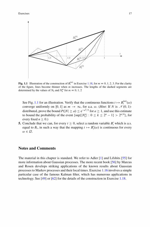
Fig. 1.1 Illustration of the construction of B.m/t in Exercise 1.18, for m D 0; 1; 2; 3. For the clarityof the figure, lines become thinner when m increases. The lengths of the dashed segments aredetermined by the values of N0 and Nm

k for m D 0; 1; 2

See Fig. 1.1 for an illustration. Verify that the continuous functions t 7! B.m/t .!/

converge uniformly on Œ0; 1� as m ! 1, for a.a. !. (Hint: If N is N .0; 1/-distributed, prove the bound P.jNj � a/ � e�a2=2 for a � 1, and use this estimateto bound the probability of the event fsupfjNn

k j W 0 � k � 2n � 1g > 2n=4g, forevery fixed n � 0.)

5. Conclude that we can, for every t � 0, select a random variable B0t which is a.s.

equal to Bt, in such a way that the mapping t 7! B0t.!/ is continuous for every

! 2 ˝ .

Notes and Comments

The material in this chapter is standard. We refer to Adler [1] and Lifshits [55] formore information about Gaussian processes. The more recent book [56] by Marcusand Rosen develops striking applications of the known results about Gaussianprocesses to Markov processes and their local times. Exercise 1.16 involves a simpleparticular case of the famous Kalman filter, which has numerous applications intechnology. See [49] or [62] for the details of the construction in Exercise 1.18.

Chapter 2Brownian Motion

In this chapter, we construct Brownian motion and investigate some of its properties.We start by introducing the “pre-Brownian motion” (this is not a canonicalterminology), which is easily defined from a Gaussian white noise on RC whoseintensity is Lebesgue measure. Going from pre-Brownian motion to Brownianmotion requires the additional property of continuity of sample paths, which isderived here via the classical Kolmogorov lemma. The end of the chapter discussesseveral properties of Brownian sample paths, and establishes the strong Markovproperty, with its classical application to the reflection principle.

2.1 Pre-Brownian Motion

Throughout this chapter, we argue on a probability space .˝;F ;P/. Most of thetime, but not always, random processes will be indexed by T D RC and take valuesin R.

Definition 2.1 Let G be a Gaussian white noise on RC whose intensity is Lebesguemeasure. The random process .Bt/t2R

C

defined by

Bt D G.1Œ0;t�/

is called pre-Brownian motion.

Proposition 2.2 Pre-Brownian motion is a centered Gaussian process with covari-ance

K.s; t/ D minfs; tg .not:/D s ^ t:


19

20 2 Brownian Motion

Proof By the definition of a Gaussian white noise, the variables Bt belong to acommon Gaussian space, and therefore .Bt/t�0 is a Gaussian process. Moreover, forevery s; t � 0,

EŒBsBt� D EŒG.Œ0; s�/G.Œ0; t�/� DZ 1

0

dr 1Œ0;s�.r/1Œ0;t�.r/ D s ^ t:

utThe next proposition gives different ways of characterizing pre-Brownian

motion.

Proposition 2.3 Let .Xt/t�0 be a (real-valued) random process. The followingproperties are equivalent:

(i) .Xt/t�0 is a pre-Brownian motion;(ii) .Xt/t�0 is a centered Gaussian process with covariance K.s; t/ D s ^ t;

(iii) X0 D 0 a.s., and, for every 0 � s < t, the random variable Xt � Xs isindependent of �.Xr; r � s/ and distributed according to N .0; t � s/;

(iv) X0 D 0 a.s., and, for every choice of 0 D t0 < t1 < � � � < tp, the variablesXti � Xti�1 , 1 � i � p are independent, and, for every 1 � i � p, the variableXti � Xti�1 is distributed according to N .0; ti � ti�1/.

Proof The fact that (i))(ii) is Proposition 2.2. Let us show that (ii))(iii). Weassume that .Xt/t�0 is a centered Gaussian process with covariance K.s; t/ D s ^ t,and we let H be the Gaussian space generated by .Xt/t�0. Then X0 is distributedaccording to N .0; 0/ and therefore X0 D 0 a.s. Then, fix s > 0 and write Hs for thevector space spanned by .Xr; 0 � r � s/, and QHs for the vector space spanned by.XsCu � Xs; u � 0/. Then Hs and QHs are orthogonal since, for r 2 Œ0; s� and u � 0,

EŒXr.XsCu � Xs/� D r ^ .s C u/� r ^ s D r � r D 0:

Noting that Hs and QHs are subspaces of H, we deduce from Theorem 1.9 that �.Hs/

and �. QHs/ are independent. In particular, if we fix t > s, the variable Xt � Xs isindependent of �.Hs/ D �.Xr; r � s/. Finally, using the form of the covariancefunction, we immediately get that Xt � Xs is distributed according to N .0; t � s/.

The implication (iii))(iv) is straightforward. Taking s D tp�1 and t D tp weobtain that Xtp � Xtp�1 is independent of .Xt1 ; : : : ;Xtp�1 /. Similarly, Xtp�1 � Xtp�2 isindependent of .Xt1 ; : : : ;Xtp�2 /, and so on. This implies that the variables Xti �Xti�1 ,1 � i � p, are independent.

Let us show that (iv))(i). It easily follows from (iv) that X is a centered Gaussianprocess. Then, if f is a step function on RC of the form f D Pn

iD1 �i 1.ti�1;ti �, where0 D t0 < t1 < t2 < � � � < tp, we set

G. f / DnX

iD1�i .Xti � Xti�1 /

2.1 Pre-Brownian Motion 21

(note that this definition of G. f / depends only on f and not on the particular waywe have written f D Pn

iD1 �i 1.ti�1;ti �). Suppose then that f and g are two stepfunctions. We can write f D Pn

iD1 �i 1.ti�1;ti� and g D PniD1 i 1.ti�1;ti � with the

same subdivision 0 D t0 < t1 < t2 < � � � < tp for f and for g (just take the union ofthe subdivisions arising in the expressions of f and g). It then follows from a simplecalculation that

EŒG. f /G.g/� DZR

C

f .t/g.t/ dt;

so that G is an isometry from the vector space of step functions on RC into theGaussian space H generated by X. Using the fact that step functions are densein L2.RC;B.RC/; dt/, we get that the mapping f 7! G. f / can be extended toan isometry from L2.RC;B.RC/; dt/ into the Gaussian space H. Finally, we haveG.Œ0; t�/ D Xt � X0 D Xt by construction. utRemark The variant of (iii) where the law of Xt � Xs is not specified but requiredto only depend on t � s is called the property of stationarity (or homogeneity) andindependence of increments. Pre-Brownian motion is thus a special case of the classof processes with stationary independent increments (under an additional regularityassumption, these processes are also called Lévy processes, see Sect. 6.5.2).

Corollary 2.4 Let .Bt/t�0 be a pre-Brownian motion. Then, for every choice of 0 Dt0 < t1 < � � � < tn, the law of the vector .Bt1 ;Bt2 ; : : : ;Btn/ has density

p.x1; : : : ; xn/ D 1

.2�/n=2p

t1.t2 � t1/ : : : .tn � tn�1/exp

��

nXiD1

.xi � xi�1/2

2.ti � ti�1/

�;

where by convention x0 D 0.

Proof The random variables Bt1 ;Bt2 � Bt1 ; : : : ;Btn � Btn�1 are independent withrespective distributions N .0; t1/;N .0; t2 � t1/; : : : ;N .0; tn � tn�1/. Hence thevector .Bt1 ;Bt2 � Bt1 ; : : : ;Btn � Btn�1 / has density

q.y1; : : : ; yn/ D 1

.2�/n=2p

t1.t2 � t1/ : : : .tn � tn�1/exp

��

nXiD1

y2i2.ti � ti�1/

�;

and the change of variables xi D y1 C � � � C yi for i 2 f1; : : : ; ng completes theargument. Alternatively we could have used Theorem 1.3 (ii). ut

Remark Corollary 2.4, together with the property B0 D 0, determines the collec-tion of finite-dimensional marginal distributions of pre-Brownian motion. Property(iv) of Proposition 2.3 shows that a process having the same finite-dimensionalmarginal distributions as pre-Brownian motion must also be a pre-Brownian motion.


Proposition 2.5 Let B be a pre-Brownian motion. Then,

(i) �B is also a pre-Brownian motion (symmetry property);(ii) for every � > 0, the process B�t D 1

�B�2t is also a pre-Brownian motion

(invariance under scaling);(iii) for every s � 0, the process B.s/t D BsCt � Bs is a pre-Brownian motion and is

independent of �.Br; r � s/ (simple Markov property).

Proof (i) and (ii) are very easy. Let us prove (iii). With the notation of the proofof Proposition 2.3, the �-field generated by B.s/ is �. QHs/, which is independent of�.Hs/ D �.Br; r � s/. To see that B.s/ is a pre-Brownian motion, it is enough toverify property (iv) of Proposition 2.3, which is immediate since B.s/ti � B.s/ti�1 DBsCti � BsCti�1 . ut

Let B be a pre-Brownian motion and let G be the associated Gaussian white noise.Note that G is determined by B: If f is a step function there is an explicit formulafor G. f / in terms of B, and one then uses a density argument. One often writes forf 2 L2.RC;B.RC/; dt/,

G. f / DZ 1

0

f .s/ dBs

and similarly

G. f 1Œ0;t�/ DZ t

0

f .s/ dBs ; G. f 1.s;t�/ DZ t

sf .r/ dBr :

This notation is justified by the fact that, if u < v,

Z v

udBs D G..u; v�/ D G.Œ0; v�/ � G.Œ0; u�/ D Bv � Bu:

The mapping f 7! R10

f .s/ dBs (that is, the Gaussian white noise G) is then calledthe Wiener integral with respect to B. Recall that

R10

f .s/dBs is distributed accordingto N .0;

R10

f .s/2ds/.Since a Gaussian white noise is not a “real” measure depending on !,

R10

f .s/dBs

is not a “real” integral depending on!. Much of what follows in this book is devotedto extending the definition of

R10

f .s/dBs to functions f that may depend on !.

2.2 The Continuity of Sample Paths

We start with a general definition. Let E be a metric space equipped with its Borel�-field.

2.2 The Continuity of Sample Paths 23

Definition 2.6 Let .Xt/t2T be a random process with values in E. The sample pathsof X are the mappings T 3 t 7! Xt.!/ obtained when fixing ! 2 ˝ . The samplepaths of X thus form a collection of mappings from T into E indexed by ! 2 ˝ .

Let B D .Bt/t�0 be a pre-Brownian motion. At the present stage, we have noinformation about the sample paths of B. We cannot even assert that these samplepaths are measurable functions. In this section, we will show that, at the cost of“slightly” modifying B, we can ensure that sample paths are continuous.

Definition 2.7 Let .Xt/t2T and . QXt/t2T be two random processes indexed by thesame index set T and with values in the same metric space E. We say that QX is amodification of X if

8t 2 T; P. QXt D Xt/ D 1:

This implies in particular that QX has the same finite-dimensional marginals as X.Thus, if X is a pre-Brownian motion, QX is also a pre-Brownian motion. On the otherhand, sample paths of QX may have very different properties from those of X. Forinstance, considering the case where T D RC and E D R, it is easy to constructexamples where all sample paths of QX are continuous whereas all sample paths of Xare discontinuous.

Definition 2.8 The process QX is said to be indistinguishable from X if there existsa negligible subset N of ˝ such that

8! 2 ˝nN; 8t 2 T; QXt.!/ D Xt.!/:

Put in a different way, QX is indistinguishable from X if

P.8t 2 T; Xt D QXt/ D 1:

(This formulation is slightly incorrect since the set f8t 2 T; Xt D QXtg need not bemeasurable.)

If QX is indistinguishable from X then QX is a modification of X. The notionof indistinguishability is however much stronger: Two indistinguishable processeshave a.s. the same sample paths. In what follows, we will always identify twoindistinguishable processes. An assertion such as “there exists a unique process suchthat . . . ” should always be understood “up to indistinguishability”, even if this is notstated explicitly.

The following observation will play an important role. Suppose that T D I is aninterval of R. If the sample paths of both X and QX are continuous (except possiblyon a negligible subset of ˝), then QX is a modification of X if and only if QX isindistinguishable from X. Indeed, if QX is a modification of X we have a.s. Xt D QXt

for every t 2 I \ Q (we throw out a countable union of negligible sets) hence a.s.Xt D QXt for every t 2 I, by a continuity argument. We get the same result if we onlyassume that the sample paths are right-continuous, or left-continuous.


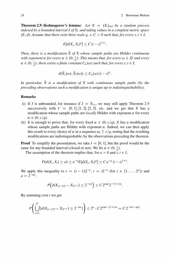
Theorem 2.9 (Kolmogorov’s lemma) Let X D .Xt/t2I be a random processindexed by a bounded interval I of R, and taking values in a complete metric space.E; d/. Assume that there exist three reals q; ";C > 0 such that, for every s; t 2 I,

EŒd.Xs;Xt/q� � C jt � sj1C":

Then, there is a modification QX of X whose sample paths are Hölder continuouswith exponent ˛ for every ˛ 2 .0; "q /: This means that, for every ! 2 ˝ and every˛ 2 .0; "q /, there exists a finite constant C˛.!/ such that, for every s; t 2 I,

d. QXs.!/; QXt.!// � C˛.!/ jt � sj˛:

In particular, QX is a modification of X with continuous sample paths (by thepreceding observations such a modification is unique up to indistinguishability).

Remarks

(i) If I is unbounded, for instance if I D RC, we may still apply Theorem 2.9successively with I D Œ0; 1�; Œ1; 2�; Œ2; 3�; etc. and we get that X has amodification whose sample paths are locally Hölder with exponent ˛ for every˛ 2 .0; "=q/.

(ii) It is enough to prove that, for every fixed ˛ 2 .0; "=q/, X has a modificationwhose sample paths are Hölder with exponent ˛. Indeed, we can then applythis result to every choice of ˛ in a sequence ˛k " "=q, noting that the resultingmodifications are indistinguishable, by the observations preceding the theorem.

Proof To simplify the presentation, we take I D Œ0; 1�, but the proof would be thesame for any bounded interval (closed or not). We fix ˛ 2 .0; "q /.

The assumption of the theorem implies that, for a > 0 and s; t 2 I,

P.d.Xs;Xt/ � a/ � a�qEŒd.Xs;Xt/q� � C a�q jt � sj1C":

We apply this inequality to s D .i � 1/2�n, t D i2�n (for i 2 f1; : : : ; 2ng) anda D 2�n˛:

P�

d.X.i�1/2�n ;Xi2�n/ � 2�n˛�

� C 2nq˛2�.1C"/n:

By summing over i we get

P

2n[

iD1fd.X.i�1/2�n ;Xi2�n/ � 2�n˛g

!� 2n � C 2nq˛�.1C"/n D C 2�n."�q˛/:


By assumption, " � q˛ > 0. Summing now over n, we obtain

1XnD1

P

2n[

iD1fd.X.i�1/2�n ;Xi2�n/ � 2�n˛g

!< 1;

and the Borel–Cantelli lemma implies that, with probability one, we can find a finiteinteger n0.!/ such that

8n � n0.!/; 8i 2 f1; : : : ; 2ng; d.X.i�1/2�n ;Xi2�n/ � 2�n˛:

Consequently the constant K˛.!/ defined by

K˛.!/ D supn�1

sup

1�i�2n

d.X.i�1/2�n ;Xi2�n/

2�n˛

!

is finite a.s. (If n � n0.!/, the supremum inside the parentheses is bounded aboveby 1, and, on the other hand, there are only finitely many terms before n0.!/.)

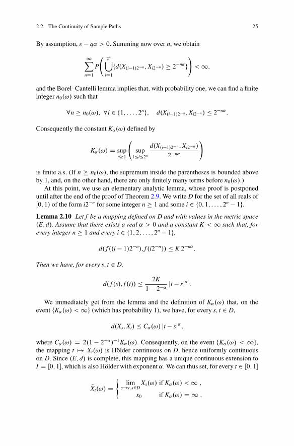
At this point, we use an elementary analytic lemma, whose proof is postponeduntil after the end of the proof of Theorem 2.9. We write D for the set of all reals ofŒ0; 1/ of the form i2�n for some integer n � 1 and some i 2 f0; 1; : : : ; 2n � 1g.

Lemma 2.10 Let f be a mapping defined on D and with values in the metric space.E; d/. Assume that there exists a real ˛ > 0 and a constant K < 1 such that, forevery integer n � 1 and every i 2 f1; 2; : : : ; 2n � 1g,

d. f ..i � 1/2�n/; f .i2�n// � K 2�n˛:

Then we have, for every s; t 2 D,

d. f .s/; f .t// � 2K

1 � 2�˛ jt � sj˛ :

We immediately get from the lemma and the definition of K˛.!/ that, on theevent fK˛.!/ < 1g (which has probability 1), we have, for every s; t 2 D,

d.Xs;Xt/ � C˛.!/ jt � sj˛;

where C˛.!/ D 2.1 � 2�˛/�1K˛.!/. Consequently, on the event fK˛.!/ < 1g,the mapping t 7! Xt.!/ is Hölder continuous on D, hence uniformly continuouson D. Since .E; d/ is complete, this mapping has a unique continuous extension toI D Œ0; 1�, which is also Hölder with exponent ˛. We can thus set, for every t 2 Œ0; 1�

QXt.!/ D(

lims!t; s2D

Xs.!/ if K˛.!/ < 1 ;

x0 if K˛.!/ D 1 ;


where x0 is a point of E which can be fixed arbitrarily. Clearly QXt is a randomvariable.

By the previous remarks, the sample paths of the process QX are Hölder withexponent ˛ on Œ0; 1�. We still need to verify that QX is a modification of X. To thisend, fix t 2 Œ0; 1�. The assumption of the theorem implies that

lims!t

Xs D Xt

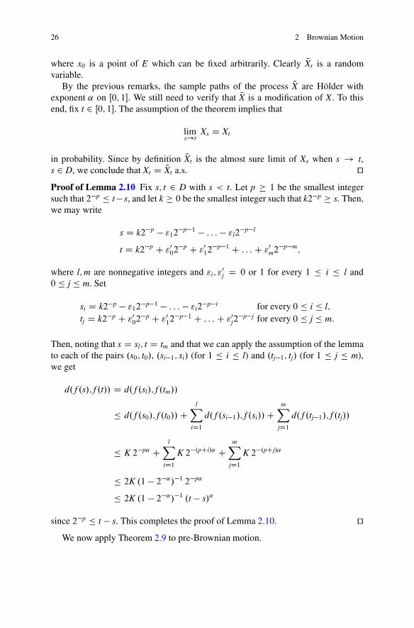
in probability. Since by definition QXt is the almost sure limit of Xs when s ! t,s 2 D, we conclude that Xt D QXt a.s. utProof of Lemma 2.10 Fix s; t 2 D with s < t. Let p � 1 be the smallest integersuch that 2�p � t� s, and let k � 0 be the smallest integer such that k2�p � s. Then,we may write

s D k2�p � "12�p�1 � : : : � "l2�p�l

t D k2�p C "002

�p C "012

�p�1 C : : :C "0m2

�p�m;

where l;m are nonnegative integers and "i; "0j D 0 or 1 for every 1 � i � l and

0 � j � m. Set

si D k2�p � "12�p�1 � : : : � "i2

�p�i for every 0 � i � l;tj D k2�p C "0

02�p C "0

12�p�1 C : : :C "0

j2�p�j for every 0 � j � m:

Then, noting that s D sl; t D tm and that we can apply the assumption of the lemmato each of the pairs .s0; t0/, .si�1; si/ (for 1 � i � l) and .tj�1; tj/ (for 1 � j � m),we get

d. f .s/; f .t// D d. f .sl/; f .tm//

� d. f .s0/; f .t0//ClX

iD1d. f .si�1/; f .si//C

mXjD1

d. f .tj�1/; f .tj//

� K 2�p˛ ClX

iD1K 2�.pCi/˛ C

mXjD1

K 2�.pCj/˛

� 2K .1 � 2�˛/�1 2�p˛

� 2K .1 � 2�˛/�1 .t � s/˛

since 2�p � t � s. This completes the proof of Lemma 2.10. utWe now apply Theorem 2.9 to pre-Brownian motion.


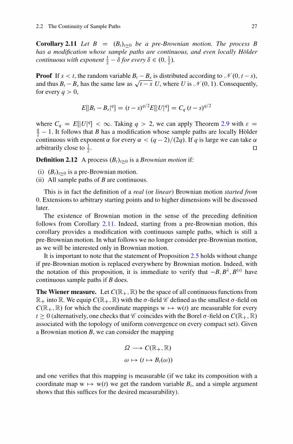
Corollary 2.11 Let B D .Bt/t�0 be a pre-Brownian motion. The process Bhas a modification whose sample paths are continuous, and even locally Höldercontinuous with exponent 1

2� ı for every ı 2 .0; 1

2/.

Proof If s < t, the random variable Bt � Bs is distributed according to N .0; t � s/,and thus Bt � Bs has the same law as

pt � s U, where U is N .0; 1/. Consequently,

for every q > 0,

EŒjBt � Bsjq� D .t � s/q=2EŒjUjq� D Cq .t � s/q=2

where Cq D EŒjUjq� < 1. Taking q > 2, we can apply Theorem 2.9 with " Dq2

� 1. It follows that B has a modification whose sample paths are locally Höldercontinuous with exponent ˛ for every ˛ < .q � 2/=.2q/. If q is large we can take ˛arbitrarily close to 1

2. ut

Definition 2.12 A process .Bt/t�0 is a Brownian motion if:

(i) .Bt/t�0 is a pre-Brownian motion.(ii) All sample paths of B are continuous.

This is in fact the definition of a real (or linear) Brownian motion started from0. Extensions to arbitrary starting points and to higher dimensions will be discussedlater.

The existence of Brownian motion in the sense of the preceding definitionfollows from Corollary 2.11. Indeed, starting from a pre-Brownian motion, thiscorollary provides a modification with continuous sample paths, which is still apre-Brownian motion. In what follows we no longer consider pre-Brownian motion,as we will be interested only in Brownian motion.

It is important to note that the statement of Proposition 2.5 holds without changeif pre-Brownian motion is replaced everywhere by Brownian motion. Indeed, withthe notation of this proposition, it is immediate to verify that �B;B�;B.s/ havecontinuous sample paths if B does.

The Wiener measure. Let C.RC;R/ be the space of all continuous functions fromRC into R. We equip C.RC;R/with the �-field C defined as the smallest �-field onC.RC;R/ for which the coordinate mappings w 7! w.t/ are measurable for everyt � 0 (alternatively, one checks that C coincides with the Borel �-field on C.RC;R/associated with the topology of uniform convergence on every compact set). Givena Brownian motion B, we can consider the mapping

˝ �! C.RC;R/

! 7! .t 7! Bt.!//

and one verifies that this mapping is measurable (if we take its composition with acoordinate map w 7! w.t/ we get the random variable Bt, and a simple argumentshows that this suffices for the desired measurability).


The Wiener measure (or law of Brownian motion) is by definition the imageof the probability measure P.d!/ under this mapping. The Wiener measure, whichwe denote by W.dw/, is thus a probability measure on C.RC;R/, and, for everymeasurable subset A of C.RC;R/, we have

W.A/ D P.B� 2 A/;

where in the right-hand side B: stands for the random continuous function t 7!Bt.!/.

We can specialize the last equality to a “cylinder set” of the form

A D fw 2 C.RC;R/ W w.t0/ 2 A0;w.t1/ 2 A1; : : : ;w.tn/ 2 Ang;

where 0 D t0 < t1 < � � � < tn, and A0;A1; : : : ;An 2 B.R/ (recall that B.R/ standsfor the Borel �-field on R). Corollary 2.4 then gives

W.fwI w.t0/ 2 A0;w.t1/ 2 A1; : : : ;w.tn/ 2 Ang/D P.Bt0 2 A0;Bt1 2 A1; : : : ;Btn 2 An/

D 1A0.0/

ZA1��An

dx1 : : : dxn

.2�/n=2p

t1.t2 � t1/ : : : .tn � tn�1/exp

��

nXiD1

.xi � xi�1/2

2.ti � ti�1/

�;

where x0 D 0 by convention.This formula for the W-measure of cylinder sets characterizes the probability

measure W. Indeed, the class of cylinder sets is stable under finite intersectionsand generates the �-field C , which by a standard monotone class argument (seeAppendix A1) implies that a probability measure on C is characterized by its valueson this class. A consequence of the preceding formula for the W-measure of cylindersets is the (fortunate) fact that the definition of the Wiener measure does not dependon the choice of the Brownian motion B: The law of Brownian motion is uniquelydefined!

Suppose that B0 is another Brownian motion. Then, for every A 2 C ,

P.B0� 2 A/ D W.A/ D P.B� 2 A/:

This means that the probability that a given property (corresponding to a measurablesubset A of C.RC;R/) holds is the same for the sample paths of B and for thesample paths of B0. We will use this observation many times in what follows (see inparticular the second part of the proof of Proposition 2.14 below).

Consider now the special choice of a probability space,

˝ D C.RC;R/; F D C ; P.dw/ D W.dw/:

2.3 Properties of Brownian Sample Paths 29

Then on this probability space, the so-called canonical process

Xt.w/ D w.t/

is a Brownian motion (the continuity of sample paths is obvious, and the fact thatX has the right finite-dimensional marginals follows from the preceding formula forthe W-measure of cylinder sets). This is the canonical construction of Brownianmotion.

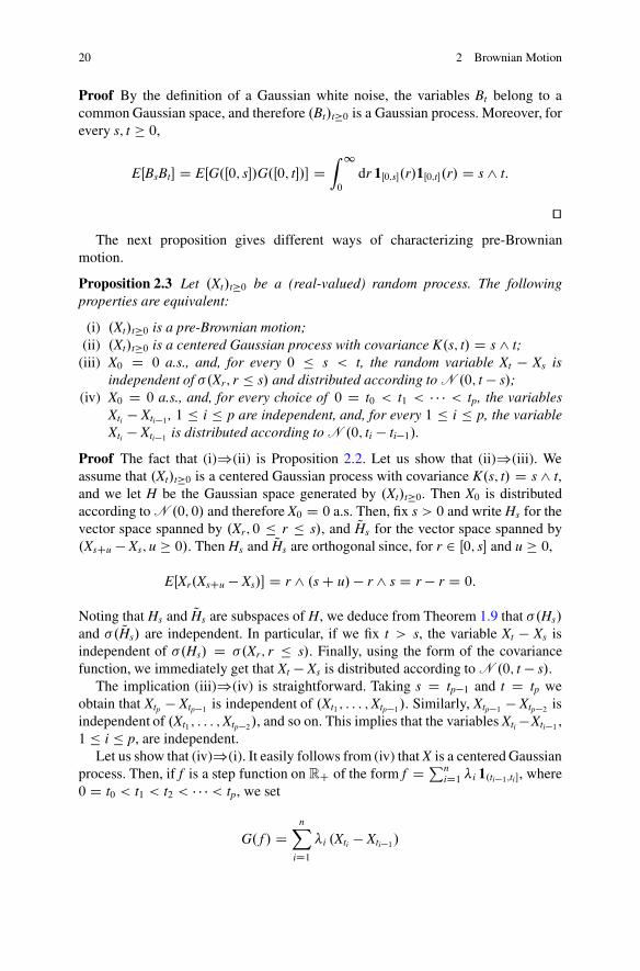
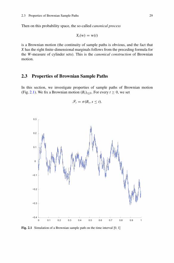
2.3 Properties of Brownian Sample Paths

In this section, we investigate properties of sample paths of Brownian motion(Fig. 2.1). We fix a Brownian motion .Bt/t�0. For every t � 0, we set

Ft D �.Bs; s � t/:

0 0.1 0.2 0.3 0.4 0.5 0.6 0.7 0.8 0.9 1−0.4

−0.3

−0.2

−0.1

0

0.1

0.2

0.3

Fig. 2.1 Simulation of a Brownian sample path on the time interval Œ0; 1�


Note that Fs � Ft if s � t. We also set

F0C D\s>0

Fs:

We start by stating a useful 0 � 1 law.

Theorem 2.13 (Blumenthal’s zero-one law) The �-field F0C is trivial, in thesense that P.A/ D 0 or 1 for every A 2 F0C.

Proof Let 0 < t1 < t2 < � � � < tk and let g W Rk �! R be a bounded continuousfunction. Also fix A 2 F0C. Then, by a continuity argument,

EŒ1A g.Bt1 ; : : : ;Btk /� D lim"#0

EŒ1A g.Bt1 � B"; : : : ;Btk � B"/�:

If 0 < " < t1, the variables Bt1 � B"; : : : ;Btk � B" are independent of F" (by thesimple Markov property of Proposition 2.5) and thus also of F0C. It follows that

EŒ1A g.Bt1 ; : : : ;Btk/� D lim"#0

P.A/EŒg.Bt1 � B"; : : : ;Btk � B"/�

D P.A/EŒg.Bt1 ; : : : ;Btk/�:

We have thus obtained that F0C is independent of �.Bt1 ; : : : ;Btk/. Since this holdsfor any finite collection ft1; : : : ; tkg of (strictly) positive reals, F0C is independent of�.Bt; t > 0/. However, �.Bt; t > 0/ D �.Bt; t � 0/ since B0 is the pointwise limitof Bt when t ! 0. Since F0C � �.Bt; t � 0/, we conclude that F0C is independentof itself, which yields the desired result. utProposition 2.14

(i) We have, a.s. for every " > 0,

sup0�s�"

Bs > 0; inf0�s�"Bs < 0:

(ii) For every a 2 R, let Ta D infft � 0 W Bt D ag (with the convention inf¿ D 1).Then,

a.s.; 8a 2 R; Ta < 1:

Consequently, we have a.s.

lim supt!1

Bt D C1; lim inft!1 Bt D �1:

Remark It is not a priori obvious that sup0�s�" Bs is measurable, since this is anuncountable supremum of random variables. However, we can take advantage of thecontinuity of sample paths to restrict the supremum to rational values of s 2 Œ0; "�,

2.3 Properties of Brownian Sample Paths 31

so that we have a supremum of a countable collection of random variables. We willimplicitly use such remarks in what follows.

Proof

(i) Let ."p/ be a sequence of positive reals strictly decreasing to 0, and let

A D\

p

nsup

0�s�"p

Bs > 0o:

Since this is a monotone decreasing intersection, it easily follows that A is F0C-measurable (we can restrict the intersection to p � p0, for any choice of p0 � 1).On the other hand,

P.A/ D limp!1 # P

�sup

0�s�"p

Bs > 0�;

and

P�

sup0�s�"p

Bs > 0�

� P.B"p > 0/ D 1

2;

which shows that P.A/ � 1=2. By Theorem 2.13 we have P.A/ D 1, hence

a:s: 8" > 0; sup0�s�"

Bs > 0:

The assertion about inf0�s�" Bs is obtained by replacing B by �B.(ii) We write

1 D P�

sup0�s�1

Bs > 0�

D limı#0

" P�

sup0�s�1

Bs > ı�;

and we use the scale invariance property (see Proposition 2.5 (ii) and thenotation of this proposition) with � D ı to see that, for every ı > 0,

P�

sup0�s�1

Bs > ı�

D P�

sup0�s�1=ı2

Bıs > 1�

D P�

sup0�s�1=ı2

Bs > 1�:

In the second equality, we use the remarks following the definition of theWiener measure to observe that the probability of the event fsup0�s�1=ı2 Bs >

1g is the same for any Brownian motion B. If we let ı go to 0, we get

P�

sups�0

Bs > 1�

D limı#0

" P�

sup0�s�1=ı2

Bs > 1�

D 1:


Then another scaling argument shows that, for every M > 0,

P�

sups�0

Bs > M�

D 1

and replacing B by �B we have also

P�

infs�0Bs < �M

�D 1:

The assertions in (ii) now follow easily. For the last one we observe that acontinuous function f W RC �! R can visit all reals only if lim supt!C1 f .t/ DC1 and lim inft!C1 f .t/ D �1.

utCorollary 2.15 Almost surely, the function t 7! Bt is not monotone on any non-trivial interval.

Proof Using assertion (i) of Proposition 2.14 and the simple Markov property, weimmediately get that a.s. for every rational q 2 QC, for every " > 0,

supq�t�qC"

Bt > Bq; infq�t�qC"Bt < Bq:

The desired result follows. Notice that we restricted ourselves to rational values of qin order to throw out a countable union of negligible sets (and by the way the resultwould fail if we had considered all real values of q). utProposition 2.16 Let 0 D tn

0 < tn1 < � � � < tn

pnD t be a sequence of subdivisions of

Œ0; t� whose mesh tends to 0 (i.e. sup1�i�pn.tn

i � tni�1/ ! 0 as n ! 1). Then,

limn!1

pnXiD1.Btni � Btni�1 /

2 D t;

in L2.

Proof This is an immediate consequence of Proposition 1.14, writing Btni� Btni�1

DG..tn

i�1; tni �/, where G is the Gaussian white noise associated with B. ut

If a < b and f is a real function defined on Œa; b�, the function f is said to haveinfinite variation if the supremum of the quantities

PpiD1 jf .ti/ � f .ti�1/j, over all

subdivisions a D t0 < t1 < � � � < tp D b, is infinite.

Corollary 2.17 Almost surely, the function t 7! Bt has infinite variation on anynon-trivial interval.

Proof From the simple Markov property, it suffices to consider the interval Œ0; t�for some fixed t > 0. We use Proposition 2.16, and note that by extracting a

2.4 The Strong Markov Property of Brownian Motion 33

subsequence we may assume that the convergence in this proposition holds a.s. Wethen observe that

pnXiD1.Btni � Btni�1

/2 ��

sup1�i�pn

jBtni � Btni�1j�

�pnX

iD1jBtni � Btni�1

j:

The supremum inside parentheses tends to 0 by the continuity of sample paths,whereas the left-hand side tends to t a.s. It follows that

PpniD1 jBtni � Btni�1 j tends to

infinity a.s., giving the desired result. utThe previous corollary shows that it is not possible to define the integralR t

0f .s/dBs as a special case of the usual (Stieltjes) integral with respect to functions

of finite variation (see Sect. 4.1.1 for a brief presentation of the integral with respectto functions of finite variation, and also the comments at the end of Sect. 2.1).

2.4 The Strong Markov Property of Brownian Motion

Our goal is to extend the simple Markov property (Proposition 2.5 (iii)) to the casewhere the deterministic time s is replaced by a random time T. We first need tospecify the class of admissible random times.

As in the previous section, we fix a Brownian motion .Bt/t�0. We keep thenotation Ft introduced before Theorem 2.13 and we also set F1 D �.Bs; s � 0/.

Definition 2.18 A random variable T with values in Œ0;1� is a stopping time if, forevery t � 0, fT � tg 2 Ft.

It is important to note that the value 1 is allowed. If T is a stopping time, wealso have, for every t > 0,

fT < tg D[

q2Œ0;t/\Q

fT � qg 2 Ft:

Examples The random variables T D t (constant stopping time) and T D Ta arestopping times (notice that fTa � tg D finf0�s�t jBs � aj D 0g). On the other hand,T D supfs � 1 W Bs D 0g is not a stopping time (arguing by contradiction, this willfollow from the strong Markov property stated below and Proposition 2.14). If T isa stopping time, then, for every t � 0, T C t is also a stopping time.

Definition 2.19 Let T be a stopping time. The �-field of the past before T is

FT D fA 2 F1 W 8t � 0; A \ fT � tg 2 Ftg:

It is easy to verify that FT is indeed a �-field, and that the random variable Tis FT -measurable. Moreover, if we define the real random variable 1fT<1gBT by


setting

1fT<1gBT.!/ D�

BT.!/.!/ if T.!/ < 1 ;

0 if T.!/ D 1 ;

then 1fT<1gBT is also FT -measurable. To see this, we first observe that

1fT<1gBTD limn!1

1XiD0

1fi2�n�T<.iC1/2�ngBi2�n D limn!1

1XiD0

1fT<.iC1/2�ng1fi2�n�TgBi2�n :

We then note that, for any s � 0, Bs1fs�Tg is FT -measurable, because if A is a Borelsubset of R not containing 0 (the case where 0 2 A is treated by considering thecomplementary event) we have

fBs1fs�Tg 2 Ag \ fT � tg D�¿ if t < sfBs 2 Ag \ fs � T � tg if t � s

which is Ft-measurable in both cases (write fs � T � tg D fT � tg \ fT < sgc).

Theorem 2.20 (strong Markov property) Let T be a stopping time. We assumethat P.T < 1/ > 0 and we set, for every t � 0,

B.T/t D 1fT<1g.BTCt � BT/:

Then under the probability measure P.� j T < 1/, the process .B.T/t /t�0 is aBrownian motion independent of FT .

Proof We first consider the case where T < 1 a.s. We fix A 2 FT and 0 � t1 <� � � < tp, and we let F be a bounded continuous function from R

p into RC. We willverify that

EŒ1A F.B.T/t1 ; : : : ;B.T/tp /� D P.A/EŒF.Bt1 ; : : : ;Btp/�: (2.1)

The different assertions of the theorem then follow. First the case A D ˝ showsthat the process .B.T/t /t�0 has the same finite-dimensional marginal distributionsas B and is thus a Brownian motion (notice that the sample paths of B.T/ arecontinuous). Then (2.1) implies that, for every choice of 0 � t1 < � � � < tp, the

vector .B.T/t1 ; : : : ;B.T/tp / is independent of FT and it follows that B.T/ is independent

of FT .Let us prove (2.1). For every integer n � 1, and for every real t � 0, we write Œt�n

for the smallest real of the form k2�n, with k 2 ZC, belonging to the interval Œt;1/.We also set Œ1�n D 1 by convention. In order to prove (2.1), we observe that wehave a.s.

F.B.T/t1 ; : : : ;B.T/tp / D lim

n!1 F.B.ŒT�n/t1 ; : : : ;B.ŒT�n/tp /;


hence by dominated convergence

EŒ1A F.B.T/t1 ; : : : ;B.T/tp /�

D limn!1 EŒ1A F.B.ŒT�n/t1 ; : : : ;B.ŒT�n/tp /�

D limn!1

1XkD0

EŒ1A1f.k�1/2�n<T�k2�ngF.Bk2�nCt1 � Bk2�n ; : : : ;Bk2�nCtp � Bk2�n/�;

where to get the last equality we have decomposed the expectation according to thepossible values of ŒT�n. The point now is the fact that, since A 2 FT , the event

A \ f.k � 1/2�n < T � k2�ng D .A \ fT � k2�ng/\ fT � .k � 1/2�ngc

is Fk2�n -measurable. By the simple Markov property (Proposition 2.5 (iii)), we havethus

EŒ1A\f.k�1/2�n<T�k2�ngF.Bk2�nCt1 � Bk2�n ; : : : ;Bk2�nCtp � Bk2�n/�

D P.A \ f.k � 1/2�n < T � k2�ng/EŒF.Bt1 ; : : : ;Btp/�;

and we just have to sum over k to get (2.1).Finally, when P.T D 1/ > 0, the same arguments give, instead of (2.1),

EŒ1A\fT<1g F.B.T/t1 ; : : : ;B.T/tp /� D P.A \ fT < 1g/EŒF.Bt1 ; : : : ;Btp/�

and the desired result again follows in a straightforward way. utAn important application of the strong Markov property is the “reflection

principle” that leads to the following theorem.

Theorem 2.21 For every t > 0, set St D sups�t Bs. Then, if a � 0 and b 2 .�1; a�,we have

P.St � a; Bt � b/ D P.Bt � 2a � b/:

In particular, St has the same distribution as jBtj.

Proof We apply the strong Markov property at the stopping time

Ta D infft � 0 W Bt D ag:


We already saw (Proposition 2.14) that Ta < 1 a.s. Then, using the notation ofTheorem 2.20, we have

P.St � a; Bt � b/ D P.Ta � t; Bt � b/ D P.Ta � t; B.Ta/t�Ta

� b � a/;

since B.Ta/t�Ta

D Bt � BTa D Bt � a on the event fTa � tg. Write B0 D B.Ta/, so that,by Theorem 2.20, the process B0 is a Brownian motion independent of FTa hencein particular of Ta. Since B0 has the same distribution as �B0, the pair .Ta;B0/ alsohas the same distribution as .Ta;�B0/ (this common distribution is just the productof the law of Ta with the Wiener measure). Let

H D f.s;w/ 2 RC � C.RC;R/ W s � t; w.t � s/ � b � ag:

The preceding probability is equal to

P..Ta;B0/ 2 H/ D P..Ta;�B0/ 2 H/

D P.Ta � t; �B.Ta/t�Ta

� b � a/

D P.Ta � t; Bt � 2a � b/

D P.Bt � 2a � b/

because the event fBt � 2a � bg is a.s. contained in fTa � tg. This gives the firstassertion (Fig. 2.2).

�

�

Ta t

a

b

2a−b

Fig. 2.2 Illustration of the reflection principle: the conditional probability, knowing that fTa � tg,that the graph is below b at time t is the same as the conditional probability that the graph reflectedat level a after time Ta (in dashed lines) is above 2a � b at time t


For the last assertion of the theorem, we observe that

P.St � a/ D P.St � a;Bt � a/C P.St � a;Bt � a/ D 2P.Bt � a/ D P.jBtj � a/;

and the desired result follows. utIt follows from the previous theorem that the law of the pair .St;Bt/ has density

g.a; b/ D 2.2a � b/p2�t3

exp

�� .2a � b/2

2t

�1fa>0;b<ag: (2.2)

Corollary 2.22 For every a > 0, Ta has the same distribution asa2

B21and has density

f .t/ D ap2�t3

exp�

� a2

2t

�1ft>0g:

Proof Using Theorem 2.21 in the second equality, we have, for every t � 0,

P.Ta � t/ D P.St � a/ D P.jBtj � a/ D P.B2t � a2/ D P.tB21 � a2/ D P.a2

B21� t/:

Furthermore, since B1 is distributed according to N .0; 1/, a straightforwardcalculation gives the density of a2=B21. utRemark From the form of the density of Ta, we immediately get that EŒTa� D 1.

We finally extend the definition of Brownian motion to the case of an arbitrary(possibly random) initial value and to any dimension.

Definition 2.23 If Z is a real random variable, a process .Xt/t�0 is a real Brownianmotion started from Z if we can write Xt D Z C Bt where B is a real Brownianmotion started from 0 and is independent of Z.

Definition 2.24 A random process Bt D .B1t ; : : : ;Bdt / with values in R

d is a d-dimensional Brownian motion started from 0 if its components B1; : : : ;Bd areindependent real Brownian motions started from 0. If Z a random variable withvalues in R

d and Xt D .X1t ; : : : ;Xdt / is a process with values in R

d, we say that X isa d-dimensional Brownian motion started from Z if we can write Xt D Z CBt whereB is a d-dimensional Brownian motion started from 0 and is independent of Z.

Note that, if X is a d-dimensional Brownian motion and the initial value of X israndom, the components of X may not be independent because the initial value mayintroduce some dependence (this does not occur if the initial value is deterministic).

In a way similar to the end of Sect. 2.2, the Wiener measure in dimensiond is defined as the probability measure on C.RC;Rd/ which is the law of a


d-dimensional Brownian motion started from 0. The canonical construction ofSect. 2.2 also applies to d-dimensional Brownian motion.

Many of the preceding results can be extended to d-dimensional Brownianmotion with an arbitrary starting point. In particular, the invariance properties ofProposition 2.5 still hold with the obvious adaptations. Furthermore, property (i)of this proposition can be extended as follows. If X is a d-dimensional Brownianmotion and ˚ is an isometry of Rd, the process .˚.Xt//t�0 is still a d-dimensionalBrownian motion. The construction of the Wiener measure and Blumenthal’s zero-one law are easily extended, and the strong Markov property also holds: One canadapt the proof of Theorem 2.20 to show that, if T is a stopping time – in the sense ofthe obvious extension of Definition 2.18 – which is finite with positive probability,then under the probability measure P.� j T < 1/, the process X.T/t D XTCt � XT ,t � 0, is a d-dimensional Brownian motion started from 0 and is independent ofFT .

Exercises

In all exercises below, .Bt/t�0 is a real Brownian motion started from 0, and St Dsup0�s�t Bs:

Exercise 2.25 (Time inversion)

1. Show that the process .Wt/t�0 defined by W0 D 0 and Wt D tB1=t for t > 0 is(indistinguishable of) a real Brownian motion started from 0. (Hint: First verifythat W is a pre-Brownian motion.)

2. Infer that limt!1

Bt

tD 0 a.s.

Exercise 2.26 For every real a � 0, we set Ta D infft � 0 W Bt D ag. Show that theprocess .Ta/a�0 has stationary independent increments, in the sense that, for every0 � a � b, the variable Tb � Ta is independent of the �-field �.Tc; 0 � c � a/ andhas the same distribution as Tb�a.

Exercise 2.27 (Brownian bridge)We set Wt D Bt � tB1 for every t 2 Œ0; 1�.

1. Show that .Wt/t2Œ0;1� is a centered Gaussian process and give its covariancefunction.

2. Let 0 < t1 < t2 < � � � < tp < 1. Show that the law of .Wt1 ;Wt2 ; : : : ;Wtp/ hasdensity

g.x1; : : : ; xp/ D p2� pt1.x1/pt2�t1 .x2 � x1/ � � � ptp�tp�1 .xp � xp�1/p1�tp.�xp/;

where pt.x/ D 1p2� t

exp.�x2=2t/. Explain why the law of .Wt1 ;Wt2 ; : : : ;Wtp/ can

be interpreted as the conditional law of .Bt1 ;Bt2 ; : : : ;Btp/ knowing that B1 D 0.

Exercises 39

3. Verify that the two processes .Wt/t2Œ0;1� and .W1�t/t2Œ0;1� have the same distribu-tion (similarly as in the definition of Wiener measure, this law is a probabilitymeasure on the space of all continuous functions from Œ0; 1� into R).

Exercise 2.28 (Local maxima of Brownian paths) Show that, a.s., the localmaxima of Brownian motion are distinct: a.s., for any choice of the rational numbersp; q; r; s � 0 such that p < q < r < s we have

supp�t�q

Bt 6D supr�t�s

Bt :

Exercise 2.29 (Non-differentiability) Using the zero-one law, show that, a.s.,

lim supt#0

Btpt

D C1 ; lim inft#0

Btpt

D �1 :

Infer that, for every s � 0, the function t 7! Bt has a.s. no right derivative at s.

Exercise 2.30 (Zero set of Brownian motion) Let H WD ft 2 Œ0; 1� W Bt D 0g. UsingProposition 2.14 and the strong Markov property, show that H is a.s. a compactsubset of Œ0; 1� with no isolated point and zero Lebesgue measure.

Exercise 2.31 (Time reversal) We set B0t D B1�B1�t for every t 2 Œ0; 1�. Show that

the two processes .Bt/t2Œ0;1� and .B0t/t2Œ0;1� have the same law (as in the definition of

Wiener measure, this law is a probability measure on the space of all continuousfunctions from Œ0; 1� into R).

Exercise 2.32 (Arcsine law)Set T WD infft � 0 W Bt D S1g:

1. Show that T < 1 a.s. (one may use the result of the previous exercise) and thenthat T is not a stopping time.

2. Verify that the three variables St, St � Bt and jBtj have the same law.3. Show that T is distributed according to the so-called arcsine law, whose density

is

g.t/ D 1

�p

t.1 � t/1.0;1/.t/:

4. Show that the results of questions 1. and 3. remain valid if T is replaced byL WD supft � 1 W Bt D 0g:

Exercise 2.33 (Law of the iterated logarithm)The goal of the exercise is to prove that

lim supt!1

Btp2t log log t

D 1 a.s.


We set h.t/ D p2t log log t:

1. Show that, for every t > 0, P.St > up

t/ � 2

up2�

e�u2=2, when u ! C1.

2. Let r and c be two real numbers such that 1 < r < c2: From the behavior of theprobabilities P.Srn > c h.rn�1// when n ! 1, infer that, a.s.,

lim supt!1

Btp2t log log t

� 1:

3. Show that a.s. there are infinitely many values of n such that

Brn � Brn�1 �r

r � 1

rh.rn/:

Conclude that the statement given at the beginning of the exercise holds.

4. What is the value of lim inft!1

Btp2t log log t

?

Notes and Comments

The first rigorous mathematical construction of Brownian motion is due toWiener [81] in 1923. We use the nonstandard terminology of “pre-Brownianmotion” to emphasize the necessity of choosing an appropriate modification inorder to get a random process with continuous sample paths. There are severalconstructions of Brownian motion from a sequence of independent Gaussianrandom variables that directly yield the continuity property, and a very elegantone is Lévy’s construction (see Exercise 1.18), which can be found in the books[49] or [62]. Lévy’s construction avoids the use of Kolmogorov’s lemma, but thelatter will have other applications in this book. We refer to Talagrand’s book [78]for far-reaching refinements of the “chaining method” used above in the proof ofKolmogorov’s lemma. Much of what we know about linear Brownian motion comesfrom Lévy, see in particular [54, Chapitre VI]. Perhaps surprisingly, the strongMarkov property of Brownian motion was proved only in the 1950s by Hunt [32](see also Dynkin [19] for a more general version obtained independently of Hunt’swork), but it had been used before by other authors, in particular by Lévy [54],without a precise justification. The reflection principle and its consequences alreadyappeared, long before Brownian motion was rigorously constructed, in Bachelier’sthesis [2], which was a pioneering work in financial mathematics. The book [62]by Mörters and Peres is an excellent source for various sample path properties ofBrownian motion.

Chapter 3Filtrations and Martingales

In this chapter, we provide a short introduction to the theory of continuous timerandom processes on a filtered probability space. On the way, we generalize severalnotions introduced in the previous chapter in the framework of Brownian motion,and we provide a thorough discussion of stopping times. In a second step, wedevelop the theory of continuous time martingales, and, in particular, we deriveregularity results for sample paths of martingales. We finally discuss the optionalstopping theorem for martingales and supermartingales, and we give applications toexplicit calculations of distributions related to Brownian motion.

3.1 Filtrations and Processes

Throughout this chapter, we consider a probability space .˝;F ;P/. In this section,we introduce some general notions that will be of constant use later.

Definition 3.1 A filtration on .˝;F ;P/ is a collection .Ft/0�t�1 indexed byŒ0;1� of sub-�-fields of F , such that Fs � Ft for every s � t � 1.

We have thus, for every 0 � s < t,

F0 � Fs � Ft � F1 � F :

We also say that .˝;F ; .Ft/;P/ is a filtered probability space

Example If B is a Brownian motion, we considered in Chap. 2 the filtration

Ft D �.Bs; 0 � s � t/; F1 D �.Bs; s � 0/:


41

42 3 Filtrations and Martingales

More generally, if X D .Xt; t � 0/ is any random process indexed by RC, thecanonical filtration of X is defined by F X

t D �.Xs; 0 � s � t/ and F X1 D�.Xs; s � 0/.

Let .Ft/0�t�1 be a filtration on .˝;F ;P/. We set, for every t � 0

FtC D\s>t

Fs;

and F1C D F1. Note that Ft � FtC for every t 2 Œ0;1�. The collection.FtC/0�t�1 is also a filtration. We say that the filtration .Ft/ is right-continuous if

FtC D Ft; 8t � 0:

By construction, the filtration .FtC/ is right-continuous.Let .Ft/ be a filtration and let N be the class of all .F1;P/-negligible sets (i.e.

A 2 N if there exists an A0 2 F1 such A � A0 and P.A0/ D 0). The filtration issaid to be complete if N � F0 (and thus N � Ft for every t).

If .Ft/ is not complete, it can be completed by setting F 0t D Ft _ �.N /, for

every t 2 Œ0;1�, using the notationFt _�.N / for the smallest �-field that containsboth Ft and �.N / (recall that �.N / is the �-field generated by N ). We willoften apply this completion procedure to the canonical filtration of a random process.Xt/t�0, and call the resulting filtration the completed canonical filtration of X. Thereader will easily check that all results stated in Chap. 2, where we were consideringthe canonical filtration of a Brownian motion B, remain valid if instead we dealwith the completed canonical filtration. The point is that augmenting a �-field withnegligible sets does not alter independence properties.

Let us turn to random processes, which in this chapter will be indexed by RC.

Definition 3.2 A process X D .Xt/t�0 with values in a measurable space .E;E / issaid to be measurable if the mapping

.!; t/ 7! Xt.!/

defined on ˝ � RC equipped with the product �-field F ˝ B.RC/ is measurable.(We recall that B.RC/ stands for the Borel �-field of R.)

This is stronger than saying that, for every t � 0, Xt is F -measurable. On theother hand, considering for instance the case where E D R, it is easy to see thatif the sample paths of X are continuous, or only right-continuous, the fact that Xt

is F -measurable for every t implies that the process is measurable in the previoussense – see the argument in the proof of Proposition 3.4 below.

In the remaining part of this chapter, we fix a filtration .Ft/ on .˝;F ;P/,and the notions that will be introduced depend on the choice of this filtration.

Definition 3.3 A random process .Xt/t�0 with values in a measurable space .E;E /is called adapted if, for every t � 0, Xt is Ft-measurable. This process is said to be

3.1 Filtrations and Processes 43

progressive if, for every t � 0, the mapping

.!; s/ 7! Xs.!/

defined on ˝ � Œ0; t� is measurable for the �-field Ft ˝ B.Œ0; t�/.

Note that a progressive process is both adapted and measurable (saying that aprocess is measurable is equivalent to saying that, for every t � 0, the mapping.!; s/ 7! Xs.!/ defined on ˝ � Œ0; t� is measurable for F ˝ B.Œ0; t�/).

Proposition 3.4 Let .Xt/t�0 be a random process with values in a metric space.E; d/ (equipped with its Borel �-field). Suppose that X is adapted and that thesample paths of X are right-continuous (i.e. for every ! 2 ˝ , t 7! Xt.!/ is right-continuous). Then X is progressive. The same conclusion holds if one replaces right-continuous by left-continuous.

Proof We treat only the case of right-continuous sample paths, as the other case issimilar. Fix t > 0. For every n � 1 and s 2 Œ0; t�, define a random variable Xn

s bysetting

Xns D Xkt=n if s 2 Œ.k � 1/t=n; kt=n/; k 2 f1; : : : ; ng;

and Xnt D Xt. The right-continuity of sample paths ensures that, for every s 2 Œ0; t�

and ! 2 ˝ ,

Xs.!/ D limn!1 Xn

s .!/:

On the other hand, for every Borel subset A of E,

f.!; s/ 2 ˝ � Œ0; t� W Xns .!/ 2 Ag D .fXt 2 Ag � ftg/

[� n[kD1

�fXkt=n 2 Ag � Œ .k � 1/t

n;

kt

n/��

which belongs to the �-field Ft ˝ B.Œ0; t�/. Hence, for every n � 1, the mapping.!; s/ 7! Xn

s .!/, defined on ˝ � Œ0; t�, is measurable for Ft ˝ B.Œ0; t�/. Since apointwise limit of measurable functions is also measurable, the same measurabilityproperty holds for the mapping .!; s/ 7! Xs.!/ defined on˝ � Œ0; t�. It follows thatthe process X is progressive. utThe progressive � -field The collection P of all sets A 2 F ˝ B.RC/ such thatthe process Xt.!/ D 1A.!; t/ is progressive forms a �-field on ˝ � RC, which iscalled the progressive �-field. A subset A of ˝ � RC belongs to P if and only if,for every t � 0, A \ .˝ � Œ0; t�/ belongs to Ft ˝ B.Œ0; t�/.

One then verifies that a process X is progressive if and only if the mapping.!; t/ 7! Xt.!/ is measurable on ˝ � RC equipped with the �-field P .


3.2 Stopping Times and Associated � -Fields

In this section, we extend certain notions that were already introduced in theprevious chapter in the framework of Brownian motion. The following definitionis just a repetition of the corresponding one in the previous chapter.

Definition 3.5 A random variable T W ˝ �! Œ0;1� is a stopping time of thefiltration .Ft/ if fT � tg 2 Ft, for every t � 0. The �-field of the past before T isthen defined by

FT D fA 2 F1 W 8t � 0; A \ fT � tg 2 Ftg:

The reader will verify that FT is indeed a �-field.In what follows, “stopping time” will mean stopping time of the filtration .Ft/

unless otherwise specified. If T is a stopping time, we also have fT < tg 2 Ft forevery t > 0, by the same argument as in the Brownian case, and moreover

fT D 1g D� 1[

nD1fT � ng

�c 2 F1:

Recall the definition of the filtration .FtC/. A stopping time (of the filtration.Ft/) is obviously also a stopping time of the filtration .FtC/, but the converseneed not be true in general.

Proposition 3.6 Write Gt D FtC for every t 2 Œ0;1�.

(i) A random variable T W ˝ �! Œ0;1� is a stopping time of the filtration .Gt/ ifand only if fT < tg 2 Ft for every t > 0. This is also equivalent to saying thatT ^ t is Ft-measurable for every t > 0.

(ii) Let T be a stopping time of the filtration .Gt/. Then

GT D fA 2 F1 W 8t > 0; A \ fT < tg 2 Ftg:

We will write

FTC WD GT :

Proof

(i) Suppose that T is a stopping time of the filtration .Gt/. Then, for every t > 0,

fT < tg D[

q2QC

; q<t

fT � qg 2 Ft

3.2 Stopping Times and Associated � -Fields 45

because fT � qg 2 Gq � Ft if q < t. Conversely, assume that fT < tg 2 Ft

for every t > 0. Then, for every t � 0 and s > t,

fT � tg D\

q2QC

; t<q<s

fT < qg 2 Fs

and it follows that fT � tg 2 FtC D Gt.Then, saying that T ^ t is Ft-measurable for every t > 0 is equivalent to

saying that, for every s < t, fT � sg 2 Ft. Taking a sequence of values of s thatincreases to t, we see that the latter property implies that fT < tg 2 Ft, and soT is a stopping time of the filtration .Gt/. Conversely, if T is a stopping time ofthe filtration .Gt/, we have fT � sg 2 Gs � Ft whenever s < t, and thus T ^ tis Ft-measurable.

(ii) First, if A 2 GT , we have A \ fT � tg 2 Gt for every t � 0. Hence, for t > 0,

A \ fT < tg D[

q2QC

; q<t

�A \ fT � qg

�2 Ft

since A \ fT � qg 2 Gq � Ft, for every q < t.Conversely, assume that A \ fT < tg 2 Ft for every t > 0. Then, for every

t � 0, and s > t,

A \ fT � tg D\

q2QC

; t<q<s

�A \ fT < qg

�2 Fs:

In this way, we get that A \ fT � tg 2 FtC D Gt and thus A 2 GT .ut

Properties of stopping times and of the associated � -fields

(a) For every stopping time T, we have FT � FTC. If the filtration .Ft/ is right-continuous, we have FTC D FT .

(b) If T D t is a constant stopping time, FT D Ft and FTC D FtC.(c) Let T be a stopping time. Then T is FT -measurable.(d) Let T be a stopping time and A 2 F1. Set

TA.!/ D�

T.!/ if ! 2 A ;C1 if ! … A :

Then A 2 FT if and only if TA is a stopping time.(e) Let S;T be two stopping times such that S � T. Then FS � FT and FSC �

FTC

.(f) Let S;T be two stopping times. Then, S _ T and S ^ T are also stopping times

and FS^T D FS \ FT . Furthermore, fS � Tg 2 FS^T and fS D Tg 2 FS^T .


(g) If .Sn/ is a monotone increasing sequence of stopping times, then S D lim " Sn

is also a stopping time.(h) If .Sn/ is a monotone decreasing sequence of stopping times, then S D lim # Sn

is a stopping time of the filtration .FtC/, and

FSC D\

n

FSnC:

(i) If .Sn/ is a monotone decreasing sequence of stopping times, which is alsostationary (in the sense that, for every !, there exists an integer N.!/ suchthat Sn.!/ D S.!/ for every n � N.!/) then S D lim # Sn is also a stoppingtime, and

FS D\

n

FSn :

( j) Let T be a stopping time. A function ! 7! Y.!/ defined on the set fT < 1gand taking values in the measurable set .E;E / is FT -measurable if and only if,for every t � 0, the restriction of Y to the set fT � tg is Ft-measurable.

Remark In property ( j) we use the (obvious) notion of G -measurability for arandom variable ! 7! Y.!/ that is defined only on a G -measurable subset of ˝(here G is a �-field on ˝). This notion will be used again in Theorem 3.7 below.

Proof (a), (b) and (c) are almost immediate from our definitions. Let us prove theother statements.

(d) For every t � 0,

fTA � tg D A \ fT � tgand the result follows from the definition of FT .

(e) It is enough to prove that FS � FT . If A 2 FS, we have

A \ fT � tg D .A \ fS � tg/ \ fT � tg 2 Ft;

hence A 2 FT .(f) We have

fS ^ T � tg D fS � tg [ fT � tg 2 Ft;

fS _ T � tg D fS � tg \ fT � tg 2 Ft;

so that S ^ T and S _ T are stopping times.It follows from (e) that FS^T � .FS \ FT/. Moreover, if A 2 FS \ FT ,

A \ fS ^ T � tg D .A \ fS � tg/ [ .A \ fT � tg/ 2 Ft;

hence A 2 FS^T .

3.2 Stopping Times and Associated � -Fields 47

Then, for every t � 0,

fS � Tg \ fT � tg D fS � tg \ fT � tg \ fS ^ t � T ^ tg 2 Ft;

fS � Tg \ fS � tg D fS ^ t � T ^ tg \ fS � tg 2 Ft;

because S ^ t and T ^ t are both Ft-measurable by Proposition 3.6 (i). It followsthat fS � Tg 2 FS \ FT D FS^T . Then fS D Tg D fS � Tg \ fT � Sg.

(g) For every t � 0,

fS � tg D\

n

fSn � tg 2 Ft:

(h) Similarly

fS < tg D[

n

fSn < tg 2 Ft;

and we use Proposition 3.6 (i). Then, by (e), we have FSC � FSnC for every n,and conversely, if A 2 Tn FSnC,

A \ fS < tg D[

n

.A \ fSn < tg/ 2 Ft;

hence A 2 FSC.(i) In that case, we also have

fS � tg D[

n

fSn � tg 2 Ft;

and if A 2 Tn FSn ,

A \ fS � tg D[

n

.A \ fSn � tg/ 2 Ft;

so that A 2 FS.( j) First assume that, for every t � 0, the restriction of Y to fT � tg is Ft-

measurable. Then, for every measurable subset A of E,

fY 2 Ag \ fT � tg 2 Ft:

Letting t ! 1, we first obtain that fY 2 Ag 2 F1, and then we deduce fromthe previous display that fY 2 Ag 2 FT .

Conversely, if Y is FT -measurable, fY 2 Ag 2 FT and thus fY 2 Ag \ fT �tg 2 Ft, giving the desired result. ut


Theorem 3.7 Let .Xt/t�0 be a progressive process with values in a measurablespace .E;E /, and let T be a stopping time. Then the function ! 7! XT.!/ WDXT.!/.!/, which is defined on the event fT < 1g, is FT-measurable.

Proof We use property ( j) above. Let t � 0. The restriction to fT � tg of thefunction ! 7! XT.!/ is the composition of the two mappings

fT � tg 3 ! 7! .!;T.!/ ^ t/

Ft Ft ˝ B.Œ0; t�/

and

˝ � Œ0; t� 3 .!; s/ 7! Xs.!/

Ft ˝ B.Œ0; t�/ E

which are both measurable (the first one since T ^ t is Ft-measurable, byProposition 3.6 (i), and the second one by the definition of a progressive process). Itfollows that the restriction to fT � tg of the function ! 7! XT.!/ is Ft-measurable,which gives the desired result by property ( j). utProposition 3.8 Let T be a stopping time and let S be an FT-measurable randomvariable with values in Œ0;1�, such that S � T. Then S is also a stopping time.

In particular, if T is a stopping time,

Tn D1X

kD0

k C 1

2n1fk2�n<T�.kC1/2�ng C 1 � 1fTD1g ; n D 0; 1; 2; : : :

defines a sequence of stopping times that decreases to T.

Proof For the first assertion, we write, for every t � 0,

fS � tg D fS � tg \ fT � tg 2 Ft

since fS � tg is FT -measurable. The second assertion follows since Tn � T, and Tn

is a function of T, hence FT -measurable, and Tn # T as n " 1 by construction. utThe following proposition will be our main tool to construct stopping times

associated with random processes.

Proposition 3.9 Let .Xt/t�0 be an adapted process with values in a metric space.E; d/.

(i) Assume that the sample paths of X are right-continuous, and let O be an opensubset of E. Then

TO D infft � 0 W Xt 2 Og

is a stopping time of the filtration .FtC/.

3.3 Continuous Time Martingales and Supermartingales 49

(ii) Assume that the sample paths of X are continuous, and let F be a closed subsetof E. Then

TF D infft � 0 W Xt 2 Fg

is a stopping time (of the filtration .Ft/).

Proof

(i) For every t > 0,

fTO < tg D[

s2Œ0;t/\Q

fXs 2 Og 2 Ft;

and we use Proposition 3.6 (i).(ii) For every t � 0,

fTF � tg Dn

inf0�s�t

d.Xs;F/ D 0o

Dn

infs2Œ0;t�\Q

d.Xs;F/ D 0o

2 Ft:

ut

3.3 Continuous Time Martingales and Supermartingales

Recall that we have fixed a filtered probability space .˝;F ; .Ft/;P/. In theremaining part of this chapter, all processes take values in R. The following is anobvious analog of the corresponding definition in discrete time (see Appendix A2below).

Definition 3.10 An adapted real-valued process .Xt/t�0 such that Xt 2 L1 for everyt � 0 is called

• a martingale if, for every 0 � s < t, EŒXt j Fs� D Xs;• a supermartingale if, for every 0 � s < t, EŒXt j Fs� � Xs;• a submartingale if, for every 0 � s < t, EŒXt j Fs� � Xs.

If .Xt/t�0 is a submartingale, .�Xt/t�0 is a supermartingale. For this reason, someof the results below are stated for supermartingales only, but the analogous resultsfor submartingales immediately follow.

If .Xt/t�0 is a martingale (resp. a supermartingale, resp. a submartingale), wehave EŒXs� D EŒXt� (resp. EŒXs� � EŒXt�, resp. EŒXs� � EŒXt�) whenever 0 � s � t.

A simple way to construct a martingale is to take a random variable Z 2 L1 andto set Xt D EŒZ j Ft� for every t � 0. Not all martingales are of this type, however.Let us turn to an important class of examples.


Important example We say that a process .Zt/t�0 with values in R or in Rd has

independent increments with respect to the filtration .Ft/ if Z is adapted and if, forevery 0 � s < t, Zt � Zs is independent of Fs (for instance, a Brownian motion hasindependent increments with respect to its canonical filtration). If Z is a real-valuedprocess having independent increments with respect to .Ft/, then

(i) if Zt 2 L1 for every t � 0, theneZt D Zt � EŒZt� is a martingale;(ii) if Zt 2 L2 for every t � 0, then Yt DeZ2t � EŒeZ2t � is a martingale;

(iii) if, for some � 2 R, we have EŒe�Zt � < 1 for every t � 0, then

Xt D e�Zt

EŒe�Zt �

is a martingale.

Proofs of these facts are very easy. In the second case, we have for every 0 � s < t,

EŒ.eZt/2 j Fs� D EŒ.eZs CeZt �eZs/

2 j Fs�

D eZ2s C 2eZsEŒeZt �eZs j Fs�C EŒ.eZt �eZs/2 j Fs�

D eZ2s C EŒ.eZt �eZs/2�

D eZ2s C EŒeZ2t � � 2EŒeZseZt�C EŒeZ2s �D eZ2s C EŒeZ2t � � EŒeZ2s �;

because EŒeZseZt� D EŒeZsEŒeZt j Fs�� D EŒeZ2s �. The desired result follows. In the thirdcase,

EŒXt j Fs� D e�Zs EŒe�.Zt�Zs/ j Fs�

EŒe�Zs �EŒe�.Zt�Zs/�D e�Zs

EŒe�Zs �D Xs;

using the fact that EŒe�.Zt�Zs/ j Fs� D EŒe�.Zt�Zs/� by independence.Consider the special case of Brownian motion.

Definition 3.11 A real-valued process B D .Bt/t�0 is an .Ft/-Brownian motionif B is a Brownian motion and if B is adapted and has independent incrementswith respect to .Ft/. Similarly, a process B D .Bt/t�0 with values in R

d is a d-dimensional .Ft/-Brownian motion if B is a d-dimensional Brownian motion and ifB is adapted and has independent increments with respect to .Ft/.

Note that if B is a (d-dimensional) Brownian motion and .F Bt / is the (possibly

completed) canonical filtration of B, then B is a (d-dimensional) .F Bt /-Brownian

motion.Let B be an .Ft/-Brownian motion started from 0 (or from any a 2 R). Then it

follows from the above observations that the processes

Bt ; B2t � t ; e�Bt� �2

2 t


are martingales with continuous sample paths. The processes e�Bt� �2

2 t are calledexponential martingales of Brownian motion

We can also take, for f 2 L2.RC;B.RC/; dt/,

Zt DZ t

0

f .s/ dBs :

Properties of Gaussian white noise imply that Z has independent increments withrespect to the canonical filtration of B, and thus

Z t

0

f .s/dBs ;� Z t

0

f .s/dBs

�2 �Z t

0

f .s/2ds ; exp��

Z t

0

f .s/dBs � �2

2

Z t

0

f .s/2ds�

are martingales (with respect to this filtration). One can prove that these martingaleshave a modification with continuous sample paths – it is enough to do it for the firstone, and this will follow from the more general results in Chap. 5 below.

Finally, if Z D N is a Poisson process with parameter� (and .Ft/ is the canonicalfiltration of N), it is well known that Z has independent increments, and we get that

Nt � �t ; .Nt � �t/2 � �t; exp.�Nt � �t.e� � 1//

are martingales. In contrast with the previous examples, these martingales do nothave a modification with continuous sample paths.

Proposition 3.12 Let .Xt/t�0 be an adapted process and let f W R �! RC be aconvex function such that EŒf .Xt/� < 1 for every t � 0.

(i) If .Xt/t�0 is a martingale, then .f .Xt//t�0 is a submartingale.(ii) If .Xt/t�0 is a submartingale, and if in addition f is nondecreasing, then

.f .Xt//t�0 is a submartingale.

Proof By Jensen’s inequality, we have, for s < t,

EŒ f .Xt/ j Fs� � f .EŒXt j Fs�/ � f .Xs/:

In the last inequality, we need the fact that f is nondecreasing when .Xt/ is only asubmartingale. utConsequences If .Xt/t�0 is a martingale, jXtj is a submartingale and more gener-ally, for every p � 1, jXtjp is a submartingale, provided that we have EŒjXtjp� < 1for every t � 0. If .Xt/t�0 is a submartingale, .Xt/

C D Xt _0 is also a submartingale.

Remark If .Xt/t�0 is any martingale, Jensen’s inequality shows that EŒjXtjp� is anondecreasing function of t with values in Œ0;1�, for every p � 1.


Proposition 3.13 Let .Xt/t�0 be a submartingale or a supermartingale. Then, forevery t > 0,

sup0�s�t

EŒjXsj� < 1:

Proof It is enough to treat the case where .Xt/t�0 is a submartingale. Since .Xt/C is

also a submartingale, we have for every s 2 Œ0; t�,EŒ.Xs/

C� � EŒ.Xt/C�:

On the other hand, since X is a submartingale, we also have for s 2 Œ0; t�,EŒXs� � EŒX0�:

By combining these two bounds, and noting that jxj D 2xC � x, we get

sups2Œ0;t�

EŒjXsj� � 2EŒ.Xt/C� � EŒX0� < 1;

giving the desired result. utThe next proposition will be very useful in the study of square integrable

martingales.

Proposition 3.14 Let .Mt/t�0 be a square integrable martingale (that is, Mt 2 L2

for every t � 0). Let 0 � s < t and let s D t0 < t1 < � � � < tp D t be a subdivisionof the interval Œs; t�. Then,

Eh pX

iD1.Mti � Mti�1 /

2ˇ̌ˇFs

iD EŒM2

t � M2s j Fs� D EŒ.Mt � Ms/

2 j Fs�:

In particular,

Eh pX

iD1.Mti � Mti�1 /

2i

D EŒM2t � M2

s � D EŒ.Mt � Ms/2�:

Proof For every i D 1; : : : ; p,

EŒ.Mti � Mti�1 /2 j Fs� D EŒEŒ.Mti � Mti�1 /

2 j Fti�1 � j Fs�

D EhEŒM2

ti j Fti�1 � � 2Mti�1 EŒMti j Fti�1 �C M2ti�1

ˇ̌ˇFs

i

D EhEŒM2

ti j Fti�1 � � M2ti�1

ˇ̌ˇFs

i

D EŒM2ti � M2

ti�1 j Fs�

and the desired result follows by summing over i. ut


Our next goal is to study the regularity properties of sample paths of martingalesand supermartingales. We first establish continuous time analogs of classicalinequalities in the discrete time setting.

Proposition 3.15

(i) (Maximal inequality) Let .Xt/t�0 be a supermartingale with right-continuoussample paths. Then, for every t > 0 and every � > 0,

�P�

sup0�s�t

jXsj > ��

� EŒjX0j�C 2EŒjXtj�:

(ii) (Doob’s inequality in Lp) Let .Xt/t�0 be a martingale with right-continuoussample paths. Then, for every t > 0 and every p > 1,

Eh

sup0�s�t

jXsjpi

�� p

p � 1

�pEŒjXtjp�:

Note that part (ii) of the proposition is useful only if EŒjXtjp� < 1.

Proof

(i) Fix t > 0 and consider a countable dense subset D of RC such that 0 2 Dand t 2 D. Then D \ Œ0; t� is the increasing union of a sequence .Dm/m�1 offinite subsets Œ0; t� of the form Dm D ftm

0 ; tm1 ; : : : ; t

mmg where 0 D tm

0 < tm1 <

� � � < tmm D t. For every fixed m, we can apply the discrete time maximal

inequality (see Appendix A2) to the sequence Yn D Xtn^m , which is a discretesupermartingale with respect to the filtration Gn D Ftn^m . We get

�P�

sups2Dm

jXsj > ��


Then, we observe that

P�

sups2Dm

jXsj > ��

" P�

sups2D\Œ0;t�

jXsj > ��

when m " 1. We have thus

�P�

sups2D\Œ0;t�

jXsj > ��


Finally, the right-continuity of sample paths (and the fact that t 2 D) ensuresthat

sups2D\Œ0;t�

jXsj D sups2Œ0;t�

jXsj: (3.1)

Assertion (i) now follows.


(ii) Following the same strategy as in the proof of (i), and using now Doob’sinequality in Lp for discrete martingales (see Appendix A2), we get, for everym � 1,

Eh

sups2Dm

jXsjpi

�� p

p � 1�p

EŒjXtjp�:

Now we just have to let m tend to infinity, using the monotone convergencetheorem and then the identity (3.1).

utRemark If we no longer assume that the sample paths of the supermartingale X areright-continuous, the preceding proof shows that, for every countable dense subsetD of RC, and every t > 0,

P�

sups2D\Œ0;t�

jXsj > ��

� 1

�.EŒjX0j�C 2EŒjXtj�/:

Letting � ! 1, we have in particular

sups2D\Œ0;t�

jXsj < 1 ; a.s.

Upcrossing numbers Let f W I �! R be a function defined on a subset I of RC. Ifa < b, the upcrossing number of f along Œa; b�, denoted by Mf

ab.I/, is the maximalinteger k � 1 such that there exists a finite increasing sequence s1 < t1 < � � � <sk < tk of elements of I such that f .si/ � a and f .ti/ � b for every i 2 f1; : : : ; kg(if, even for k D 1, there is no such subsequence, we take Mf

ab.I/ D 0, and if such asubsequence exists for every k � 1, we take Mf

ab.I/ D 1). Upcrossing numbers area convenient tool to study the regularity of functions.

In the next lemma, the notation

lims##t

f .s/ .resp. lims""t

f .s/ /

means

lims#t;s>t

f .s/ .resp. lims"t;s<t

f .s/ /:

We say that g W RC ! R is càdlàg (for the French “continue à droite avec deslimites à gauche”) if g is right-continuous and has left-limits at every t > 0.

Lemma 3.16 Let D be a countable dense subset of RC and let f be a real functiondefined on D. We assume that, for every T 2 D,

(i) the function f is bounded on D \ Œ0;T�;(ii) for all rationals a and b such that a < b,

Mfab.D \ Œ0;T�/ < 1:


Then, the right-limit

f .tC/ WD lims##t;s2D

f .s/

exists for every real t � 0, and similarly the left-limit

f .t�/ WD lims""t;s2D

f .s/

exists for every real t > 0. Furthermore, the function g W RC �! R defined byg.t/ D f .tC/ is càdlàg.

We omit the proof of this analytic lemma. It is important to note that the right andleft-limits f .tC/ and f .t�/ are defined for every t � 0 (t > 0 in the case of f .t�/)and not only for t 2 D.

Theorem 3.17 Let .Xt/t�0 be a supermartingale, and let D be a countable densesubset of RC.

(i) For almost every ! 2 ˝ , the restriction of the function s 7! Xs.!/ to the set Dhas a right-limit

XtC.!/ WD lims##t;s2D

Xs.!/ (3.2)

at every t 2 Œ0;1/, and a left-limit

Xt�.!/ WD lims""t;s2D

Xs.!/

at every t 2 .0;1/.(ii) For every t 2 RC, XtC 2 L1 and

Xt � EŒXtC j Ft�;

with equality if the function t �! EŒXt� is right-continuous (in particular if Xis a martingale). The process .XtC/t�0 is a supermartingale with respect to thefiltration .FtC/. It is a martingale if X is a martingale.

Remark For the last assertions of (ii), we need XtC.!/ to be defined for every! 2 ˝ and not only outside a negligible set. As we will see in the proof, we canjust take XtC.!/ D 0 when the limit in (3.2) does not exist.

Proof

(i) Fix T 2 D. By the remark following Proposition 3.15, we have

sups2D\Œ0;T�

jXsj < 1 ; a.s.


As in the proof of Proposition 3.15, we can choose a sequence .Dm/m�1 offinite subsets of D that increase to D \ Œ0;T� and are such that 0;T 2 Dm.Doob’s upcrossing inequality for discrete supermartingales (see Appendix A2)gives, for every a < b and every m � 1,

EŒMXab.Dm/� � 1

b � aEŒ.XT � a/��:

We let m ! 1 and get by monotone convergence

EŒMXab.D \ Œ0;T�/� � 1

b � aEŒ.XT � a/�� < 1:

We thus have

MXab.Œ0;T� \ D/ < 1 ; a.s.

Set

N D[T2D

�nsup

t2D\Œ0;T�jXtj D 1

o[� [a;b2Q;a<b

fMXab.D \ Œ0;T�/ D 1g

��:

(3.3)

Then P.N/ D 0 by the preceding considerations. On the other hand, if ! … N,the function D 3 t 7! Xt.!/ satisfies all assumptions of Lemma 3.16. Assertion(i) now follows from this lemma.

(ii) To define XtC.!/ for every ! 2 ˝ and not only on ˝nN, we set

XtC.!/ D(

lims##t;s2D

Xs.!/ if the limit exists

0 otherwise.

With this definition, XtC is FtC-measurable.Fix t � 0 and choose a sequence .tn/n�0 in D such that tn decreases strictly

to t as n ! 1. Then, by construction, we have a.s.

XtC D limn!1 Xtn :

Set Yk D Xt�k for every integer k � 0. Then Y is a backward super-

martingale with respect to the (backward) discrete filtration Hk D Ft�k (see

Appendix A2). From Proposition 3.13, we have supk�0 EŒjYkj� < 1. Theconvergence theorem for backward supermartingales (see Appendix A2) thenimplies that the sequence Xtn converges to XtC in L1. In particular, XtC 2 L1.

Thanks to the L1-convergence, we can pass to the limit n ! 1 in theinequality Xt � EŒXtn j Ft�, and we get

Xt � EŒXtC

j Ft�


(we use the fact that the conditional expectation is continuous for the L1-norm,and it is important to realize that an a.s. convergence would not be sufficientto warrant this passage to the limit). Furthermore, thanks again to the L1-convergence, we have EŒXtC� D lim EŒXtn �. Thus, if the function s �! EŒXs�

is right-continuous, we must have EŒXt� D EŒXtC� D EŒEŒXtC

j Ft��, and theinequality Xt � EŒXt

C

j Ft� then forces Xt D EŒXtC

j Ft�.We already noticed that XtC is FtC-measurable. Let s < t and let .sn/n�0

be a sequence in D that decreases strictly to s. We may assume that sn � tn forevery n. Then as previously Xsn converges to XsC in L1, and thus, if A 2 FsC,which implies A 2 Fsn for every n, we have

EŒXsC1A�D limn!1 EŒXsn 1A� � lim

n!1 EŒXtn 1A�D EŒXtC1A� D EŒEŒXtC j FsC�1A�:

Since this inequality holds for every A 2 FsC, and since XsC and EŒXtC j FsC�are both FsC-measurable, it follows that XsC � EŒXtC j FsC� . Finally, ifX is a martingale, inequalities can be replaced by equalities in the previousconsiderations.

utTheorem 3.18 Assume that the filtration .Ft/ is right-continuous and complete.Let X D .Xt/t�0 be a supermartingale, such that the function t �! EŒXt� is right-continuous. Then X has a modification with càdlàg sample paths, which is also an.Ft/-supermartingale.

Proof Let D be a countable dense subset of RC as in Theorem 3.17. Let N be thenegligible set defined in (3.3). We set, for every t � 0,

Yt.!/ D�

XtC.!/ if ! … N0 if ! 2 N:

Lemma 3.16 then shows that the sample paths of Y are càdlàg.The random variable XtC is FtC-measurable, and thus Ft-measurable since

the filtration is right-continuous. As the negligible set N belongs to F1, thecompleteness of the filtration ensures that Yt is Ft-measurable. By Theorem 3.17(ii), we have for every t � 0,

Xt D EŒXtC j Ft� D XtC D Yt; a:s:

because XtC is Ft-measurable. Consequently, Y is a modification of X. The processY is adapted to the filtration .Ft/. Since Y is a modification of X the inequalityEŒXt j Fs� � Xs, for 0 � s < t, implies that the same inequality holds for Y. utRemarks

(i) Let us comment on the assumptions of the theorem. A simple example showsthat our assumption that the filtration is right-continuous is necessary. Take


˝ D f�1; 1g, with the probability measure P defined by P.f1g/ D P.f�1g/ D1=2. Let " be the random variable ".!/ D !, and let the process .Xt/t�0 bedefined by Xt D 0 if 0 � t � 1, and Xt D " if t > 1. Then it is easy to verifythat X is a martingale with respect to its canonical filtration .F X

t / (which iscomplete since there are no nonempty negligible sets!). On the other hand, nomodification of X can be right-continuous at t D 1. This does not contradict thetheorem since the filtration is not right-continuous (F X

1C 6D F X1 ).

(ii) Similarly, to show that the right-continuity of the mapping t �! EŒXt� isneeded, we can just take Xt D f .t/, where f is any nonincreasing deterministicfunction. If f is not right-continuous, no modification of X can have right-continuous sample paths.

3.4 Optional Stopping Theorems

We start with a convergence theorem for supermartingales.

Theorem 3.19 Let X be a supermartingale with right-continuous sample paths.Assume that the collection .Xt/t�0 is bounded in L1. Then there exists a randomvariable X1 2 L1 such that

limt!1 Xt D X1; a.s.

Proof Let D be a countable dense subset of RC. From the proof of Theorem 3.17,we have, for every T 2 D and a < b,

EŒMXab.D \ Œ0;T�/� � 1

b � aEŒ.XT � a/��:

By monotone convergence, we get, for every a < b,

EŒMXab.D/� � 1

b � asupt�0

EŒ.Xt � a/�� < 1;

since the collection .Xt/t�0 is bounded in L1. Hence, a.s. for all rationals a < b, wehave MX

ab.D/ < 1. This implies that the limit

X1 WD limD3t!1 Xt (3.4)

exists a.s. in Œ�1;1�. We can in fact exclude the values C1 and �1, sinceFatou’s lemma gives

EŒjX1j� � lim infD3t!1 EŒjXtj� < 1;

3.4 Optional Stopping Theorems 59

and we get that X1 2 L1. The right-continuity of sample paths (which we have notyet used) allows us to remove the restriction t 2 D in the limit (3.4). ut

Under the assumptions of Theorem 3.19, the convergence of Xt towards X1 maynot hold in L1. The next result gives, in the case of a martingale, necessary andsufficient conditions for the convergence to also hold in L1.

Definition 3.20 A martingale .Xt/t�0 is said to be closed if there exists a randomvariable Z 2 L1 such that, for every t � 0,

Xt D EŒZ j Ft�:

Theorem 3.21 Let X be a martingale with right-continuous sample paths. Then thefollowing properties are equivalent:

(i) X is closed;(ii) the collection .Xt/t�0 is uniformly integrable;

(iii) Xt converges a.s. and in L1 as t ! 1.

Moreover, if these properties hold, we have Xt D EŒX1 j Ft� for every t � 0, whereX1 2 L1 is the a.s. limit of Xt as t ! 1.

Proof The fact that (i))(ii) is easy: If Z 2 L1, the collection of all random variablesEŒZ j G �, when G varies over sub-�-fields of F , is uniformly integrable. If (ii)holds, in particular the collection .Xt/t�0 is bounded in L1 and Proposition 3.19implies that Xt converges a.s. to X1. By uniform integrability, the latter convergencealso holds in L1. Finally, if (iii) holds, for every s � 0, we can pass to the limit t !1 in the equality Xs D EŒXt j Fs� (using the fact that the conditional expectation iscontinuous for the L1-norm), and we get Xs D EŒX1 j Fs�. ut

We will now use the optional stopping theorems for discrete martingales andsupermartingales in order to establish similar results in the continuous time setting.Let .Xt/t�0 be a martingale or a supermartingale with right-continuous sample paths,and such that Xt converges a.s. as t ! 1 to a random variable denoted by X1. Then,for every stopping time T, we write XT for the random variable

XT.!/ D 1fT.!/<1gXT.!/.!/C 1fT.!/D1gX1.!/:

Compare with Theorem 3.7, where the random variable XT was only defined onthe subset fT < 1g of ˝ . With this definition, the random variable XT is stillFT -measurable: Use Theorem 3.7 and the easily verified fact that 1fTD1gX1 isFT -measurable.

Theorem 3.22 (Optional stopping theorem for martingales) Let .Xt/t�0 be auniformly integrable martingale with right-continuous sample paths. Let S and T betwo stopping times with S � T. Then XS and XT are in L1 and

XS D EŒXT j FS�:


In particular, for every stopping time S, we have

XS D EŒX1 j FS�;

and

EŒXS� D EŒX1� D EŒX0�:

Proof Set, for every integer n � 0,

Tn D1X

kD0

k C 1

2n1fk2�n<T�.kC1/2�ng C 1 � 1fTD1g

and similarly

Sn D1X

kD0

k C 1

2n1fk2�n<S�.kC1/2�ng C 1 � 1fSD1g:

By Proposition 3.8, .Tn/ and .Sn/ are two sequences of stopping times that decreaserespectively to T and to S. Moreover, we have Sn � Tn for every n � 0.

Now observe that, for every fixed n, 2nSn and 2nTn are stopping times of thediscrete filtration H

.n/k WD Fk=2n , and Y.n/k WD Xk=2n is a discrete martingale

with respect to this filtration. From the optional stopping theorem for uniformlyintegrable discrete martingales (see Appendix A2) we get that Y.n/2nSn

and Y.n/2nTnare in

L1, and

XSn D Y.n/2nSnD EŒY.n/2nTn

j H .n/2nSn� D EŒXTn j FSn �

(here we need to verify that H .n/2nSn

D FSn , but this is straightforward).Let A 2 FS. Since FS � FSn , we have A 2 FSn and thus

EŒ1AXSn � D EŒ1AXTn �:

By the right-continuity of sample paths, we get a.s.

XS D limn!1 XSn ; XT D lim

n!1 XTn :

These limits also hold in L1. Indeed, thanks again to the optional stopping theoremfor uniformly integrable discrete martingales, we have XSn D EŒX1 j FSn � for everyn, and thus the sequence .XSn/ is uniformly integrable (and the same holds for thesequence .XTn/).


The L1-convergence implies that XS and XT belong to L1, and also allows us topass to the limit n ! 1 in the equality EŒ1AXSn � D EŒ1AXTn � in order to get

EŒ1A XS� D EŒ1A XT �:

Since this holds for every A 2 FS, and since the variable XS is FS-measurable (bythe remarks before the theorem), we conclude that

XS D EŒXT j FS�;

which completes the proof. utWe now give two corollaries of Theorem 3.22.

Corollary 3.23 Let .Xt/t�0 be a martingale with right-continuous sample paths,and let S � T be two bounded stopping times. Then XS and XT are in L1 and

XS D EŒXT j FS� :

Proof Let a � 0 such that S � T � a. We apply Theorem 3.22 to the martingale.Xtâ/t�0 which is closed by Xa. ut

The second corollary shows that a martingale (resp. a uniformly integrablemartingale) stopped at an arbitrary stopping time remains a martingale (resp. auniformly integrable martingale). This result will play an important role in the nextchapters.

Corollary 3.24 Let .Xt/t�0 be a martingale with right-continuous sample paths,and let T be a stopping time.

(i) The process .Xt^T/t�0 is still a martingale.(ii) Suppose in addition that the martingale .Xt/t�0 is uniformly integrable. Then

the process .Xt^T/t�0 is also a uniformly integrable martingale, and moreprecisely we have for every t � 0,

Xt^T D EŒXT j Ft�: (3.5)

Proof We start with the proof of (ii). Note that t ^ T is a stopping time by property(f) of stopping times. By Theorem 3.22, Xt^T and XT are in L1, and we also knowthat Xt^T is Ft^T -measurable, hence Ft-measurable since Ft^T � Ft. So in orderto get (3.5), it is enough to prove that, for every A 2 Ft,

EŒ1A XT � D EŒ1A Xt^T �:

Let us fix A 2 Ft. First, we have trivially

EŒ1A\fT�tg XT � D EŒ1A\fT�tg Xt^T �: (3.6)


On the other hand, by Theorem 3.22, we have

Xt^T D EŒXT j Ft^T �;

and we notice that we have both A \ fT > tg 2 Ft and A \ fT > tg 2 FT (the latteras a straightforward consequence of the definition of FT ), so that A \ fT > tg 2Ft \ FT D Ft^T . Using the preceding display, we obtain

EŒ1A\fT>tg XT � D EŒ1A\fT>tg Xt^T �:

By adding this equality to (3.6), we get the desired result.To prove (i), we just need to apply (ii) to the (uniformly integrable) martingale

.Xtâ/a�0, for any choice of a � 0. utApplications Above all, the optional stopping theorem is a powerful tool forexplicit calculations of probability distributions. Let us give a few important andtypical examples of such applications (several other examples can be found in theexercises of this and the following chapters). Let B be a real Brownian motion startedfrom 0. We know that B is a martingale with continuous sample paths with respectto its canonical filtration. For every real a, set Ta D infft � 0 W Bt D ag. Recall thatTa < 1 a.s.

(a) Law of the exit point from an interval. For every a < 0 < b, we have

P.Ta < Tb/ D b

b � a; P.Tb < Ta/ D �a

b � a:

To get this result, consider the stopping time T D Ta ^ Tb and the stoppedmartingale Mt D Bt^T (this is a martingale by Corollary 3.24). Then, jMj isbounded above by b _ jaj, and the martingale M is thus uniformly integrable.We can apply Theorem 3.22 and we get

0 D EŒM0� D EŒMT � D b P.Tb < Ta/C a P.Ta < Tb/:

Since we also have P.Tb < Ta/CP.Ta < Tb/ D 1, the desired result follows. Infact the proof shows that the result remains valid if we replace Brownian motionby a martingale with continuous sample paths and initial value 0, provided weknow that this process exits .a; b/ a.s.

(b) First moment of exit times. For every a > 0, consider the stopping time Ua Dinfft � 0 W jBtj D ag. Then

EŒUa� D a2:

To verify this, consider the martingale Mt D B2t � t. By Corollary 3.24,MtÛa is still a martingale, and therefore EŒMtÛa � D EŒM0� D 0, givingEŒ.BtÛa/

2� D EŒt ^ Ua�. Then, on one hand, EŒt ^ Ua� converges to EŒUa� as


t ! 1 by monotone convergence, on the other hand, EŒ.BtÛa/2� converges to

EŒ.BUa/2� D a2 as t ! 1, by dominated convergence (note that .BtÛa/

2 � a2).The stated result follows. We may observe that we have EŒUa� < 1 in contrastwith the property EŒTa� D 1, which was noticed in Chap. 2.

(c) Laplace transform of hitting times. We now fix a > 0 and our goal is to computethe Laplace transform of Ta. For every � 2 R, we can consider the exponentialmartingale

N�t D exp.�Bt � �2

2t/:

Suppose first that � > 0. By Corollary 3.24, the stopped process N�t^Ta

is stilla martingale, and we immediately see that this martingale is bounded above bye�a, hence uniformly integrable. By applying the last assertion of Theorem 3.22to this martingale and to the stopping time S D Ta (or to S D 1) we get

e�aEŒe� �2

2 Ta � D EŒN�Ta� D EŒN�

0 � D 1 :

Replacing � byp2�, we conclude that, for every � > 0,

EŒe��Ta � D e�ap2�: (3.7)

(This formula could also be deduced from the knowledge of the density of Ta,see Corollary 2.22.) As an instructive example, one may try to reproduce thepreceding line of reasoning, using now the martingale N�

t for � < 0: one getsan absurd result, which can be explained by the fact that the stopped martingaleN�

t^Tais not uniformly integrable when � < 0. When applying Theorem 3.22,

it is crucial to always verify the uniform integrability of the martingale. In mostcases, this is done by verifying that the (stopped) martingale is bounded.

(d) Laplace transform of exit times from an interval. With the notation of (b), wehave for every a > 0 and every � > 0,

EŒexp.��Ua/� D 1

cosh.ap2�/

:

To see this, first note that Ua and BUa are independent since, using the symmetryproperty of Brownian motion,

EŒ1fBUa Dag exp.��Ua/� D EŒ1fBUa D�ag exp.��Ua/� D 1

2EŒexp.��Ua/�:

Then the claimed formula is proved by the same method as in (c), writingEŒN�

Ua� D EŒN�

0 � D 1 and noting that the application of the optional stopping


theorem is justified by the fact that N�tÛa

is bounded above by e�a. See alsoExercise 3.27 for a more general formula.

We end this chapter with the optional stopping theorem for nonnegative super-martingales. This result will be useful in later applications to Markov processes.We first note that, if .Zt/t�0 is a nonnegative supermartingale with right-continuoussample paths, .Zt/t�0 is automatically bounded in L1 since EŒZt� � EŒZ0�, and byTheorem 3.19, Zt converges a.s. to a random variable Z1 2 L1 as t ! 1. Asexplained before Theorem 3.22, we can thus make sense of ZT for any (finite or not)stopping time T.

Theorem 3.25 Let .Zt/t�0 be a nonnegative supermartingale with right-continuoussample paths. Let U and V be two stopping times such that U � V. Then, ZU andZV are in L1, and

ZU � EŒZV j FU�:

Remark This implies that EŒZU� � EŒZV �, and since ZU D ZV D Z1 on the eventfU D 1g, it also follows that

EŒ1fU<1g ZU� � EŒ1fU<1g ZV � � EŒ1fV<1g ZV �:

Proof In the first step of the proof, we make the extra assumption that U and V arebounded and we verify that we then have EŒZU� � EŒZV �. Let p � 1 be an integersuch that U � p and V � p. For every integer n � 0, set

Un Dp2n�1XkD0

k C 1

2n1fk2�n<U�.kC1/2�ng ; Vn D

p2n�1XkD0

k C 1

2n1fk2�n<V�.kC1/2�ng

in such a way (by Proposition 3.8) that .Un/ and .Vn/ are two sequences of boundedstopping times that decrease respectively to U and V , and additionally we have Un �Vn for every n � 0. The right-continuity of sample paths ensures that ZUn �! ZU

and ZVn �! ZV a.s. as n ! 1. Then, by the optional stopping theorem for discretesupermartingales in the case of bounded stopping times (see Appendix A2), withrespect to the filtration .Fk=2nC1 /k�0, we have for every n � 0,

ZUnC1� EŒZUn j FUnC1

�:

Setting Yn D ZU�n and Hn D FU

�n , for every integer n � 0, we get thatthe sequence .Yn/n�0 is a backward supermartingale with respect to the filtration.Hn/n�0. Since, for every n � 0, EŒZUn � � EŒZ0� (by another application of thediscrete optional stopping theorem), the sequence .Yn/n�0 is bounded in L1, andby the convergence theorem for backward supermartingales (see Appendix A2), itconverges in L1. Hence the convergence of ZUn to ZU also holds in L1 and similarly

Exercises 65

the convergence of ZVn to ZV holds in L1. Since Un � Vn, by yet another applicationof the discrete optional stopping theorem, we have EŒZUn � � EŒZVn �. Using theL1-convergence of ZUn and ZVn we can pass to the limit n ! 1 and obtain thatEŒZU� � EŒZV � as claimed.

Let us prove the statement of the theorem (no longer assuming that U and V arebounded). By the first step of the proof applied to the stopping times 0 and U ^p, wehave EŒZU^p� � EŒZ0� for every p � 1, and Fatou’s lemma gives EŒZU� � EŒZ0� <1 and similarly EŒZV � < 1. Fix A 2 FU � FV and recall our notation UA forthe stopping time defined by UA.!/ D U.!/ if ! 2 A and UA.!/ D 1 otherwise(cf. property (d) of stopping times). By the first part of the proof, we have, for everyp � 1,

EŒZUA^p� � EŒZVA^p�:

By writing each of these two expectations as a sum of expectations over the sets Ac,A \ fU � pg and A \ fU > pg, and noting that U > p implies V > p, we get

EŒZU 1A\fU�pg� � EŒZV 1A\fU�pg�:

Letting p ! 1 then gives

EŒZU 1A\fU<1g� � EŒZV 1A\fU<1g�:

On the other hand, the equality EŒZU 1A\fUD1g� D EŒZV 1A\fUD1g� is trivial andby adding it to the preceding display, we obtain

EŒZU 1A� � EŒZV 1A� D EŒEŒZV j FU� 1A�:

Since this holds for every A 2 FU and ZU is FU-measurable, the desired resultfollows. ut

Exercises

In the following exercises, processes are defined on a probability space .˝;F ;P/equipped with a complete filtration .Ft/t2Œ0;1�.

Exercise 3.26

1. Let M be a martingale with continuous sample paths such that M0 D x 2 RC.We assume that Mt � 0 for every t � 0, and that Mt ! 0 when t ! 1, a.s.Show that, for every y > x,

P�

supt�0

Mt � y�

D x

y:


2. Give the law of

supt�T0

Bt

when B is a Brownian motion started from x > 0 and T0 D infft � 0 W Bt D 0g.3. Assume now that B is a Brownian motion started from 0, and let > 0. Using

an appropriate exponential martingale, show that

supt�0.Bt � t/

is exponentially distributed with parameter 2.

Exercise 3.27 Let B be an .Ft/-Brownian motion started from 0. Recall thenotation Tx D infft � 0 W Bt D xg, for every x 2 R. We fix two real numbersa and b with a < 0 < b, and we set

T D Ta ^ Tb :

1. Show that, for every � > 0,

EŒexp.��T/� D cosh. bCa2

p2�/

cosh. b�a2

p2�/

:

(Hint: One may consider a martingale of the form

Mt D exp�p

2�.Bt � ˛/ � �t�

C exp�

�p2�.Bt � ˛/ � �t

�

with a suitable choice of ˛.)2. Show similarly that, for every � > 0,

EŒexp.��T/ 1fTDTag� D sinh.bp2�/

sinh..b � a/p2�/

:

3. Recover the formula for P.Ta < Tb/ from question (2).

Exercise 3.28 Let .Bt/t�0 be an .Ft/-Brownian motion started from 0. Let a > 0

and

�a D infft � 0 W Bt � t � ag:

1. Show that �a is a stopping time and that �a < 1 a.s.

Exercises 67

2. Using an appropriate exponential martingale, show that, for every � � 0,

EŒexp.��a/� D exp.�a.p1C 2�� 1//:

The fact that this formula remains valid for � 2 Œ� 12; 0Œ can be obtained via an

argument of analytic continuation.

3. Let 2 R and Mt D exp.Bt � 2

2t/. Show that the stopped martingale M�a^t

is closed if and only if � 1. (Hint: This martingale is closed if and only ifEŒM�a � D 1.)

Exercise 3.29 Let .Yt/t�0 be a uniformly integrable martingale with continuoussample paths, such that Y0 D 0. We set Y1 D limt!1 Yt. Let p � 1 be a fixedreal number. We say that Property (P) holds for the martingale Y if there exists aconstant C such that, for every stopping time T, we have

EŒjY1 � YT jp j FT � � C:

1. Show that Property (P) holds for Y if Y1 is bounded.2. Let B be an .Ft/-Brownian motion started from 0. Show that Property (P) holds

for the martingale Yt D Bt^1. (Hint: One may observe that the random variablesupt�1 jBtj is in Lp.)

3. Show that Property (P) holds for Y, with the constant C, if and only if, for anystopping time T,

EŒjYT � Y1jp� � C PŒT < 1�:

(Hint: It may be useful to consider the stopping times TA defined for A 2 FT inproperty (d) of stopping times.)

4. We assume that Property (P) holds for Y with the constant C. Let S be astopping time and let YS be the stopped martingale defined by YS

t D Yt^S (seeCorollary 3.24). Show that Property (P) holds for YS with the same constantC. One may start by observing that, if S and T are stopping times, one hasYS

T D YS^T D YTS D EŒYT j FS�.

5. We assume in this question and the next one that Property (P) holds for Y withthe constant C D 1. Let a > 0, and let .Rn/n�0 be the sequence of stopping timesdefined by induction by

R0 D 0 ; RnC1 D infft � Rn W jYt � YRn j � ag .inf¿ D 1/:

Show that, for every integer n � 0,

ap P.RnC1 < 1/ � P.Rn < 1/:


6. Infer that, for every x > 0,

P�

supt�0

Yt > x�

� 2p 2�px=2:

Notes and Comments

This chapter gives a brief presentation of the so-called general theory of processes.We limited ourselves to the notions that are needed in the remaining part ofthis book, but the interested reader can consult the treatise of Dellacherie andMeyer [13, 14] for more about this subject. Most of the martingale theory presentedin Sections 3 and 4 goes back to Doob [15]. A comprehensive study of the theory ofcontinuous time martingales can be found in [14]. The applications of the optionalstopping theorem to Brownian motion are very classical. For other applications inthe same vein, see in particular the book [70] by Revuz and Yor. Exercise 3.29 istaken from the theory of BMO martingales, see e.g. [18, Chapter 7].

Chapter 4Continuous Semimartingales

Continuous semimartingales provide the general class of processes with continuoussample paths for which we will develop the theory of stochastic integration inthe next chapter. By definition, a continuous semimartingale is the sum of acontinuous local martingale and a (continuous) finite variation process. In thepresent chapter, we study separately these two classes of processes. We startwith some preliminaries about deterministic functions with finite variation, beforeconsidering the corresponding random processes. We then define (continuous) localmartingales and we construct the quadratic variation of a local martingale, whichwill play a fundamental role in the construction of stochastic integrals. We explainhow properties of a local martingale are related to those of its quadratic variation.Finally, we introduce continuous semimartingales and their quadratic variationprocesses.

4.1 Finite Variation Processes

In this chapter, all processes are indexed by RC and take real values. The first sectionprovides a brief presentation of finite variation processes. We start by discussingfunctions with finite variation in a deterministic setting.

4.1.1 Functions with Finite Variation

In our discussion of functions with finite variation, we restrict our attention tocontinuous functions, as this is the case of interest in the subsequent developments.Recall that a signed measure on a compact interval Œ0;T� is the difference of twofinite positive measures on Œ0;T�.


69

70 4 Continuous Semimartingales

Definition 4.1 Let T � 0. A continuous function a W Œ0;T��!R such that a.0/D 0

is said to have finite variation if there exists a signed measure on Œ0;T� such thata.t/ D .Œ0; t�/ for every t 2 Œ0;T�.

The measure is then determined uniquely by a. Since a is continuous anda.0/ D 0, it follows that has no atoms.

Remark The general definition of a function with finite variation does not requirecontinuity nor the condition a.0/ D 0. We impose these two conditions forconvenience.

The decomposition of as a difference of two finite positive measures on Œ0;T�is not unique, but there exists a unique decomposition D C � � such thatC and � are supported on disjoint Borel sets. To get the existence of such adecomposition, start from an arbitrary decomposition D 1�2, set D 1C2and then use the Radon–Nikodym theorem to find two nonnegative Borel functionsh1 and h2 on Œ0;T� such that

1.dt/ D h1.t/ .dt/; 2.dt/ D h2.t/ .dt/:

Then, if h.t/ D h1.t/ � h2.t/, we have

.dt/ D h.t/ .dt/ D h.t/C .dt/� h.t/� .dt/;

which gives the decomposition D C�� with C.dt/ D h.t/C .dt/,�.dt/ Dh.t/� .dt/, and the measures C and � are supported respectively on the disjointBorel sets DC D ft W h.t/ > 0g and D� D ft W h.t/ < 0g. The uniqueness of thisdecomposition D C � � follows from the fact that we have necessarily, forevery A 2 B.Œ0;T�/,

C.A/ D supf.C/ W C 2 B.Œ0;T�/; C � Ag:

We write jj for the (finite) positive measure jj D C C �. The measure jjis called the total variation of a. We have j.A/j � jj.A/ for every A 2 B.Œ0;T�/.Moreover, the Radon–Nikodym derivative of with respect to jj is

d

djj D 1DC

� 1D�

:

The fact that a.t/ D C.Œ0; t�/ � �.Œ0; t�/ shows that a is the differenceof two monotone nondecreasing continuous functions that vanish at 0 (since has no atoms, the same holds for C of �). Conversely, the difference of twomonotone nondecreasing continuous functions that vanish at 0 has finite variationin the sense of the previous definition. Indeed, this follows from the well-known factthat the formula g.t/ D �.Œ0; t�/, t 2 Œ0;T� induces a bijection between monotonenondecreasing right-continuous functions g W Œ0;T� �! RC and finite positivemeasures � on Œ0;T�.

4.1 Finite Variation Processes 71

Let f W Œ0;T� �! R be a measurable function such thatRŒ0;T� j f .s/j jj.ds/ < 1.

We set

Z T

0

f .s/ da.s/ DZŒ0;T�

f .s/ .ds/;Z T

0

f .s/ jda.s/j DZŒ0;T�

f .s/ jj.ds/:

Then the bound

ˇ̌ˇ̌Z T

0

f .s/ da.s/

ˇ̌ˇ̌ �

Z T

0

j f .s/j jda.s/j

holds. By restricting a to Œ0; t� (which amounts to restricting , C, �), wecan define

R t0

f .s/ da.s/ for every t 2 Œ0;T�, and we observe that the functiont 7! R t

0 f .s/ da.s/ also has finite variation on Œ0;T� (the associated measure is just0.ds/ D f .s/.ds/).

Proposition 4.2 For every t 2 .0;T�,Z t

0

jda.s/j D sup

(pX

iD1ja.ti/� a.ti�1/j

);

where the supremum is over all subdivisions 0 D t0 < t1 < � � � < tp D t of Œ0; t�.More precisely, for any increasing sequence 0 D tn

0 < tn1 < � � � < tn

pnD t of

subdivisions of Œ0; t� whose mesh tends to 0, we have

limn!1

pnXiD1

ja.tni / � a.tn

i�1/j DZ t

0

jda.s/j:

Remark In the usual presentation of functions with finite variation, one starts fromthe property that the supremum in the first display of the proposition is finite.

Proof Clearly, it is enough to treat the case t D T. The inequality � in the firstassertion is very easy since, for any subdivision 0 D t0 < t1 < � � � < tp D T ofŒ0;T�,

ja.ti/� a.ti�1/j D j..ti�1; ti�/j � jj..ti�1; ti�/; 8i 2 f1; : : : ; pg;

and

pXiD1

jj..ti�1; ti�/ D jj.Œ0; t�/ DZ T

0

jda.s/j:


In order to get the reverse inequality, it suffices to prove the second assertion. Sowe consider an increasing sequence 0 D tn

0 < tn1 < � � � < tn

pnD T of subdivisions

of Œ0;T�, whose mesh maxftni � tn

i�1 W 1 � i � png tends to 0. Although we areproving a “deterministic” result, we will use a martingale argument. Leaving asidethe trivial case where jj D 0, we introduce the probability space˝ D Œ0;T�, whichis equipped with the Borel �-field B D B.Œ0;T�/ and the probability measureP.ds/ D .jj.Œ0;T�//�1jj.ds/. On this probability space, we consider the discretefiltration .Bn/n�0 such that, for every integer n � 0, Bn is the �-field generated bythe intervals .tn

i�1; tni �, 1 � i � pn. We then set

X.s/ D 1DC

.s/ � 1D�

.s/ D d

djj .s/;

and, for every n � 0,

Xn D EŒX j Bn�:

Properties of conditional expectation show that Xn is constant on every interval.tn

i�1; tni � and takes the value

..tni�1; tn

i �/

jj..tni�1; tn

i �/D a.tn

i /� a.tni�1/

jj..tni�1; tn

i �/

on this interval. On the other hand, the sequence .Xn/ is a closed martingale, withrespect to the discrete filtration .Bn/. Since X is measurable with respect to B DW

n Bn, this martingale converges to X in L1, by the convergence theorem for closeddiscrete martingales (see Appendix A2). In particular,

limn!1 EŒjXnj� D EŒjXj� D 1;

where the last equality is clear since jX.s/j D 1, jj.ds/ a.e. The desired resultfollows by noting that

EŒjXnj� D .jj.Œ0;T�//�1pnX

iD1ja.tn

i / � a.tni�1/j;

and recalling that jj.Œ0;T�/ D R T0

jda.s/j. utWe now give a useful approximation lemma for the integral of a continuous

function with respect to a function with finite variation.

4.1 Finite Variation Processes 73

Lemma 4.3 If f W Œ0;T� �! R is a continuous function, and if 0 D tn0 < tn

1 < � � � <tnpn

D T is a sequence of subdivisions of Œ0;T� whose mesh tends to 0, we have

Z T

0

f .s/ da.s/ D limn!1

pnXiD1

f .tni�1/ .a.tn

i / � a.tni�1//:

Proof Let fn be defined on Œ0;T� by fn.s/ D f .tni�1/ if s 2 .tn

i�1; tni �, 1 � i � pn, and

fn.0/ D f .0/. Then,

pnXiD1

f .tni�1/ .a.tn

i / � a.tni�1// D

ZŒ0;T�

fn.s/ .ds/;

and the desired result follows by dominated convergence since fn.s/ �! f .s/ asn ! 1, for every s 2 Œ0;T�. ut

We say that a function a W RC �! R is a finite variation function on RC if therestriction of a to Œ0;T� has finite variation on Œ0;T�, for every T > 0. Then there isa unique �-finite (positive) measure on RC whose restriction to every interval Œ0;T�is the total variation measure of the restriction of a to Œ0;T�, and we write

Z 1

0

f .s/ jda.s/j

for the integral of a nonnegative Borel function f on RC with respect to this �-finitemeasure. Furthermore, we can define

Z 1

0

f .s/da.s/ D limT!1

Z T

0

f .s/da.s/ 2 .�1;1/

for any real Borel function f on RC such thatR10

j f .s/jjda.s/j < 1.

4.1.2 Finite Variation Processes

We now consider random variables and processes defined on a filtered probabilityspace .˝;F ; .Ft/;P/.

Definition 4.4 An adapted process A D .At/t�0 is called a finite variation processif all its sample paths are finite variation functions on RC. If in addition the samplepaths are nondecreasing functions, the process A is called an increasing process.

Remark In particular, A0 D 0 and the sample paths of A are continuous – onecan define finite variation processes with càdlàg sample paths, but in this bookwe consider only the case of continuous sample paths. Our special convention


that the initial value of a finite variation process is 0 will be convenient for certainuniqueness statements.

If A is a finite variation process, the process

Vt DZ t

0

jdAsj

is an increasing process. Indeed, it is clear that the sample paths of V arenondecreasing functions (as well as continuous functions that vanish at t D 0). Thefact that Vt is an Ft-measurable random variable can be deduced from the secondpart of Proposition 4.2. Writing At D 1

2.Vt C At/� 1

2.Vt � At/ shows that any finite

variation process can be written as the difference of two increasing processes (theconverse is obvious).

Proposition 4.5 Let A be a finite variation process, and let H be a progressiveprocess such that

8t � 0; 8! 2 ˝;Z t

0

jHs.!/j jdAs.!/j < 1:

Then the process H � A D ..H � A/t/t�0 defined by

.H � A/t DZ t

0

Hs dAs

is also a finite variation process.

Proof By the observations preceding the statement of Proposition 4.2, we knowthat the sample paths of H � A are finite variation functions. It remains to verifythat the process H � A is adapted. To this end, it is enough to check that, if t > 0

is fixed, if h W ˝ � Œ0; t� �! R is measurable for the �-field Ft ˝ B.Œ0; t�/, andifR t0

jh.!; s/jjdAs.!/j < 1 for every !, then the variableR t0

h.!; s/dAs.!/ is Ft-measurable.

If h.!; s/ D 1.u;v�.s/1 .!/ with .u; v� � Œ0; t� and 2 Ft, the resultis immediate since

R t0

h.!; s/dAs.!/ D 1 .!/ .Av.!/ � Au.!// in that case. Amonotone class argument (see Appendix A1) then gives the case h D 1G, G 2Ft ˝ B.Œ0; t�/. Finally, in the general case, we observe that we can write h as apointwise limit of a sequence of simple functions (i.e. finite linear combinations ofindicator functions of measurable sets) hn such that jhnj � jhj for every n, and thatwe then have

R t0

hn.!; s/dAs.!/ �! R t0

h.!; s/dAs.!/ by dominated convergence,for every ! 2 ˝ . ut

4.2 Continuous Local Martingales 75

Remarks

(i) It happens frequently that instead of the assumption of the proposition we havethe weaker assumption

a:s: 8t � 0;

Z t

0

jHs.!/j jdAs.!/j < 1:

If the filtration is complete, we can still define H � A as a finite variation processunder this weaker assumption. We replace H by the process H0 defined by

H0t.!/ D

�Ht.!/ if

R n0

jHs.!/j jdAs.!/j < 1; 8n ;0 otherwise.

Thanks to the fact that the filtration is complete, the process H0 is stillprogressive, which allows us to define H �A D H0 �A. We will use this extensionof Proposition 4.5 implicitly in what follows.

(ii) Under appropriate assumptions (if H and K are progressive andR t0

jHsj jdAsj <1,

R t0 jHsKsj jdAsj < 1 for every t � 0), we have the “associativity” property

K � .H � A/ D .KH/ � A: (4.1)

This indeed follows from the analogous deterministic result saying informallythat k.s/ .h.s/ .ds// D .k.s/h.s// .ds/ if h.s/ and k.s/h.s/ are integrable withrespect to the signed measure on Œ0; t�.

An important special case of the proposition is the case where At D t. If H is aprogressive process such that

8t � 0; 8! 2 ˝;Z t

0

jHs.!/j ds < 1;

the processR t0

Hs ds is a finite variation process.

4.2 Continuous Local Martingales

We consider again a filtered probability space .˝;F ; .Ft/;P/. If T is a stoppingtime, and if X D .Xt/t�0 is an adapted process with continuous sample paths, wewill write XT for process X stopped at T, defined by XT

t D Xt^T for every t � 0. It isuseful to observe that, if S is another stopping time,

.XT/S D .XS/T D XS^T :


Definition 4.6 An adapted process M D .Mt/t�0 with continuous sample pathsand such that M0 D 0 a.s. is called a continuous local martingale if there exists anondecreasing sequence .Tn/n�0 of stopping times such that Tn " 1 (i.e. Tn.!/" 1for every !) and, for every n, the stopped process MTn is a uniformly integrablemartingale.

More generally, when we do not assume that M0 D 0 a.s., we say that M isa continuous local martingale if the process Nt D Mt � M0 is a continuous localmartingale.

In all cases, we say that the sequence of stopping times .Tn/ reduces M if Tn " 1and, for every n, the stopped process MTn is a uniformly integrable martingale.

Remarks

(i) We do not require in the definition of a continuous local martingale thatthe variables Mt are in L1 (compare with the definition of martingales). Inparticular, the variable M0 may be any F0-measurable random variable.

(ii) Any martingale with continuous sample paths is a continuous local martingale(see property (a) below) but the converse is false, and for this reason we willsometimes speak of “true martingales” to emphasize the difference with localmartingales. Let us give a few examples of continuous local martingales whichare not (true) martingales. If B is an .Ft/-Brownian motion started from 0,and Z is an F0-measurable random variable, the process Mt D Z C Bt isalways a continuous local martingale, but is not a martingale if EŒjZj� D 1.If we require the property M0 D 0, we can also consider Mt D ZBt, which isalways a continuous local martingale (see Exercise 4.22) but is not a martingaleif EŒjZj� D 1. For a less artificial example, we refer to question (8) ofExercise 5.33.

(iii) One can define a notion of local martingale with càdlàg sample paths. In thiscourse, however, we consider only continuous local martingales.

The following properties are easily established.

Properties of continuous local martingales.

(a) A martingale with continuous sample paths is a continuous local martingale,and the sequence Tn D n reduces M.

(b) In the definition of a continuous local martingale starting from 0, one canreplace “uniformly integrable martingale” by “martingale” (indeed, one canthen observe that MTn^n is uniformly integrable, and we still have Tn ^ n " 1).

(c) If M is a continuous local martingale, then, for every stopping time T, MT is acontinuous local martingale (this follows from Corollary 3.24).

(d) If .Tn/ reduces M and if .Sn/ is a sequence of stopping times such that Sn " 1,then the sequence .Tn ^ Sn/ also reduces M (use Corollary 3.24 again).

4.2 Continuous Local Martingales 77

(e) The space of all continuous local martingales is a vector space (to check stabilityunder addition, note that if M and M0 are two continuous local martingales suchthat M0 D 0 and M0

0 D 0, if the sequence .Tn/ reduces M and if the sequence.T 0

n/ reduces M0, property (d) shows that the sequence Tn ^T 0n reduces M CM0).

The next proposition gives three other useful properties of local martingales.

Proposition 4.7

(i) A nonnegative continuous local martingale M such that M0 2 L1 is asupermartingale.

(ii) A continuous local martingale M such that there exists a random variable Z 2L1 with jMtj � Z for every t � 0 (in particular a bounded continuous localmartingale) is a uniformly integrable martingale.

(iii) If M is a continuous local martingale and M0 D 0 (or more generally M0 2L1), the sequence of stopping times

Tn D infft � 0 W jMtj � ng

reduces M.

Proof

(i) Write Mt D M0 C Nt. By definition, there exists a sequence .Tn/ of stoppingtimes that reduces N. Then, if s � t, we have for every n,

Ns^Tn D EŒNt^Tn j Fs�:

We can add on both sides the random variable M0 (which is F0-measurableand in L1 by assumption), and we get

Ms^Tn D EŒMt^Tn j Fs�:

Since M takes nonnegative values, we can now let n tend to 1 and apply theversion of Fatou’s lemma for conditional expectations, which gives

Ms � EŒMt j Fs�:

Taking s D 0, we get EŒMt� � EŒM0� < 1, hence Mt 2 L1 for every t � 0.The previous inequality now shows that M is a supermartingale.

(ii) By the same argument as in (i), we get for 0 � s � t,

Ms^Tn D EŒMt^Tn j Fs�: (4.2)

Since jMt^Tn j � Z, we can use dominated convergence to obtain that thesequence Mt^Tn converges to Mt in L1. We can thus pass to the limit n ! 1in (4.2), and get that Ms D EŒMt j Fs�.


(iii) Suppose that M0 D 0. The random times Tn are stopping times by Proposi-tion 3.9. The desired result is an immediate consequence of (ii) since MTn is acontinuous local martingale and jMTn j � n. If we only assume that M0 2 L1,we observe that MTn is dominated by n C jM0j. ut

Remark Considering property (ii) of the proposition, one might expect that acontinuous local martingale M such that the collection .Mt/t�0 is uniformlyintegrable (or even a continuous local martingale satisfying the stronger propertyof being bounded in Lp for some p > 1) is automatically a martingale. This isincorrect!! For instance, if B is a three-dimensional Brownian motion started fromx 6D 0, the process Mt D 1=jBtj is a continuous local martingale bounded in L2, butis not a martingale: see Exercise 5.33.

Theorem 4.8 Let M be a continuous local martingale. Assume that M is also afinite variation process (in particular M0 D 0). Then Mt D 0 for every t � 0, a.s.

Proof Set

�n D infft � 0 WZ t

0

jdMsj � ng

for every integer n � 0. By Proposition 3.9, �n is a stopping time (recall thatR t0 jdMsj

is an increasing process if M is a finite variation process).Fix n � 0 and set N D M�n . Note that, for every t � 0,

jNtj D jMt^�n j �Z t^�n

0

jdMsj � n:

By Proposition 4.7, N is a (bounded) martingale. Let t > 0 and let 0 D t0 < t1 <� � � < tp D t be any subdivision of Œ0; t�. Then, from Proposition 3.14, we have

EŒN2t � D

pXiD1

EŒ.Nti � Nti�1 /2�

� Eh�

sup1�i�p

jNti � Nti�1 j� pX

iD1jNti � Nti�1 j

i

� n Eh

sup1�i�p

jNti � Nti�1 ji

noting thatR t0 jdNsj � n by the definition of �n, and using Proposition 4.2.

We now apply the preceding bound to a sequence 0 D tk0 < tk

1 < � � � < tkpk

D t ofsubdivisions of Œ0; t� whose mesh tends to 0. Using the continuity of sample paths,

4.3 The Quadratic Variation of a Continuous Local Martingale 79

and the fact that N is bounded (to justify dominated convergence), we get

limk!1 E

hsup1�i�pk

jNtki� Ntki�1

ji

D 0:

We then conclude that EŒN2t � D 0, hence Mt^�n D 0 a.s. Letting n tend to 1, we get

that Mt D 0 a.s. ut

4.3 The Quadratic Variation of a Continuous LocalMartingale

From now on until the end of this chapter (and in the next chapter), we assume thatthe filtration .Ft/ is complete. The next theorem will play a very important role inforthcoming developments.

Theorem 4.9 Let M D .Mt/t�0 be a continuous local martingale. There exists anincreasing process denoted by .hM;Mit/t�0, which is unique up to indistinguisha-bility, such that M2

t � hM;Mit is a continuous local martingale. Furthermore, forevery fixed t > 0, if 0 D tn

0 < tn1 < � � � < tn

pnD t is an increasing sequence of

subdivisions of Œ0; t� with mesh tending to 0, we have

hM;Mit D limn!1

pnXiD1.Mtni � Mtni�1

/2 (4.3)

in probability. The process hM;Mi is called the quadratic variation of M.

Let us immediately mention an important special case. If M D B is an .Ft/-Brownian motion (see Definition 3.11) then B is a martingale with continuoussample paths, hence a continuous local martingale. Then by comparing (4.3) withProposition 2.16, we get that, for every t � 0,

hB;Bit D t:

So the quadratic variation of a Brownian motion is the simplest increasing processone can imagine.

Remarks

(i) We observe that the process hM;Mi does not depend on the initial value M0,but only on the increments of M: if Mt D M0 C Nt, we have hM;Mi D hN;Ni.This is obvious from the second assertion of the theorem, and this will also beclear from the proof that follows.

(ii) In the second assertion of the theorem, it is in fact not necessary to assume thatthe sequence of subdivisions is increasing.


Proof We start by proving the first assertion. Uniqueness is an easy consequenceof Theorem 4.8. Indeed, let A and A0 be two increasing processes satisfying thecondition given in the statement. Then the process At � A0

t D .M2t � A0

t/� .M2t � At/

is both a continuous local martingale and a finite variation process. It follows thatA � A0 D 0.

In order to prove existence, consider first the case where M0 D 0 and M isbounded (hence M is a true martingale, by Proposition 4.7 (ii)). Fix K > 0 and anincreasing sequence 0 D tn

0 < tn1 < � � � < tn

pnD K of subdivisions of Œ0;K� with

mesh tending to 0.We observe that, for every 0 � r < s and for every bounded Fr-measurable

variable Z, the process

Nt D Z.Ms^t � Mr^t/

is a martingale (the reader is invited to write down the easy proof!). It follows that,for every n, the process

Xnt D

pnXiD1

Mtni�1 .Mtni ^t � Mtni�1^t/

is a (bounded) martingale. The reason for considering these martingales comes fromthe following identity, which results from a simple calculation: for every n, for everyj 2 f0; 1; : : : ; png,

M2tnj

� 2Xntnj

DjX

iD1.Mtni � Mtni�1 /

2: (4.4)

Lemma 4.10 We have

limn;m!1 EŒ.Xn

K � XmK /2� D 0:

Proof of the lemma Let us fix n � m and evaluate the product EŒXnKXm

K �. Thisproduct is equal to

pnXiD1

pmXjD1

EŒMtni�1 .Mtni � Mtni�1 /Mtmj�1 .Mtmj � Mtmj�1 /�:

In this double sum, the only terms that may be nonzero are those correspondingto indices i and j such that the interval .tm

j�1; tmj � is contained in .tn

i�1; tni �. Indeed,

suppose that tni � tm

j�1 (the symmetric case tmj � tn

i�1 is treated in an analogous way).


Then, conditioning on the �-field Ftmj�1, we have

EŒMtni�1.Mtni

� Mtni�1/Mtmj�1

.Mtmj� Mtmj�1

/�

D EŒMtni�1.Mtni � Mtni�1

/Mtmj�1EŒMtmj � Mtmj�1

j Ftmj�1�� D 0:

For every j D 1; : : : ; pm, write in;m. j/ for the unique index i such that .tmj�1; tm

j � �.tn

i�1; tni �. It follows from the previous considerations that

EŒXnKXm

K � DX

1�j�pm ; iDin;m. j/

EŒMtni�1 .Mtni � Mtni�1 /Mtmj�1 .Mtmj � Mtmj�1 /�:

In each term EŒMtni�1 .Mtni � Mtni�1 /Mtmj�1 .Mtmj � Mtmj�1 /�, we can now decompose

Mtni � Mtni�1 DX

kWin;m.k/Di

.Mtmk � Mtmk�1/

and we observe that, if k is such that in;m.k/ D i but k 6D j,

EŒMtni�1 .Mtmk � Mtmk�1/Mtmj�1 .Mtmj � Mtmj�1 /� D 0

(condition on Ftmk�1if k > j and on Ftmj�1

if k < j). The only case that remains isk D j, and we have thus obtained

EŒXnKXm

K � DX

1�j�pm; iDin;m. j/

EŒMtni�1Mtmj�1 .Mtmj � Mtmj�1 /2�:

As a special case of this relation, we have

EŒ.XmK /2� D

X1�j�pm

EŒM2tmj�1.Mtmj � Mtmj�1

/2�:

Furthermore,

EŒ.XnK/2� D

X1�i�pn

EŒM2tni�1.Mtni

� Mtni�1/2�

DX1�i�pn

EŒM2tni�1

EŒ.Mtni � Mtni�1 /2 j Ftni�1 ��

DX1�i�pn

EhM2

tni�1

XjWin;m. j/Di

EŒ.Mtmj � Mtmj�1 /2 j Ftni�1 �

i

DX

1�j�pm; iDin;m. j/

EŒM2tni�1.Mtmj � Mtmj�1 /

2�;

where we have used Proposition 3.14 in the third equality.


If we combine the last three displays, we get

EŒ.XnK � Xm

K /2� D E

h X1�j�pm; iDin;m. j/

.Mtni�1 � Mtmj�1 /2 .Mtmj � Mtmj�1 /

2i:

Using the Cauchy–Schwarz inequality, we then have

EŒ.XnK � Xm

K /2� � E

hsup

1�j�pm; iDin;m. j/.Mtni�1 � Mtmj�1 /

4i1=2

� Eh� X

1�j�pm

.Mtmj � Mtmj�1 /2�2i1=2

:

By the continuity of sample paths (together with the fact that the mesh of oursubdivisions tends to 0) and dominated convergence, we have

limn;m!1; n�m

Eh

sup1�j�pm; iDin;m. j/

.Mtni�1 � Mtmj�1 /4i

D 0:

To complete the proof of the lemma, it is then enough to prove the existence of afinite constant C such that, for every m,

Eh� X

1�j�pm

.Mtmj � Mtmj�1/2�2i � C: (4.5)

Let A be a constant such that jMtj � A for every t � 0. Expanding the square andusing Proposition 3.14 twice, we have

Eh� X

1�j�pm

.Mtmj � Mtmj�1 /2�2i

D Eh X1�j�pm

.Mtmj � Mtmj�1/4i

C 2Eh X1�j<k�pm

.Mtmj � Mtmj�1/2.Mtmk � Mtmk�1

/2i

� 4A2Eh X1�j�pm

.Mtmj� Mtmj�1

/2i

C2pm�1XjD1

Eh.Mtmj

� Mtmj�1/2E

h pmXkDjC1

.Mtmk� Mtmk�1

/2ˇ̌ˇFtmj

ii

D 4A2Eh X1�j�pm

.Mtmj � Mtmj�1 /2i

C2pm�1XjD1

Eh.Mtmj � Mtmj�1 /

2 EŒ.MK � Mtmj /2 j Ftmj �

i


� 12A2 Eh X1�j�pm

.Mtmj � Mtmj�1 /2i

D 12A2 EŒ.MK � M0/2�

� 48A4

which gives the bound (4.5) with C D 48A4. This completes the proof. utWe now return to the proof of the theorem. Thanks to Doob’s inequality in L2

(Proposition 3.15 (ii)), and to Lemma 4.10, we have

limn;m!1 E

hsupt�K.Xn

t � Xmt /2i

D 0: (4.6)

In particular, for every t 2 Œ0;K�, .Xnt /n�1 is a Cauchy sequence in L2 and thus

converges in L2. We want to argue that the limit yields a process Y indexed by Œ0;K�with continuous sample paths. To see this, we note that (4.6) allows us find a strictlyincreasing sequence .nk/k�1 of positive integers such that, for every k � 1,

Eh

supt�K.X

nkC1t � Xnk

t /2i

� 2�k:

This implies that

Eh 1X

kD1supt�K

jXnkC1t � Xnk

t ji< 1

and thus

1XkD1

supt�K

jXnkC1t � Xnk

t j < 1 ; a.s.

Consequently, except on the negligible set N where the series in the last displaydiverges, the sequence of random functions .Xnk

t ; 0 � t � K/ converges uniformlyon Œ0;K� as k ! 1, and the limiting random function is continuous by uniformconvergence. We can thus set Yt.!/ D lim Xnk

t .!/, for every t 2 Œ0;K�, if ! 2˝nN , and Yt.!/ D 0, for every t 2 Œ0;K�, if ! 2 N . The process .Yt/0�t�K

has continuous sample paths and Yt is Ft-measurable for every t 2 Œ0;K� (here weuse the fact that the filtration is complete, which ensures that N 2 Ft for everyt � 0). Furthermore, since the L2-limit of .Xn

t /n�1 must coincide with the a.s. limitof a subsequence, Yt is also the limit of Xn

t in L2, for every t 2 Œ0;K�, and we canpass to the limit in the martingale property for Xn, to obtain that EŒYt j Fs� D Ys

for every 0 � s � t � K. It follows that .Yt^K/t�0 is a martingale with continuoussample paths.


On the other hand, the identity (4.4) shows that the sample paths of the processM2

t �2Xnt are nondecreasing along the finite sequence .tn

i ; 0 � i � pn/. By passing tothe limit n ! 1 along the sequence .nk/k�1, we get that the sample paths of M2

t �2Yt are nondecreasing on Œ0;K�, except maybe on the negligible set N . For everyt 2 Œ0;K�, we set A.K/t D M2

t � 2Yt on ˝nN , and A.K/t D 0 on N . Then A.K/0 D0, A.K/t is Ft-measurable for every t 2 Œ0;K�, A.K/ has nondecreasing continuoussample paths, and .M2

t^K � A.K/t^K/t�0 is a martingale.We apply the preceding considerations with K D `, for every integer ` � 1,

and we get a process .A.`/t /0�t�`. We then observe that, for every ` � 1, A.`C1/t^` DA.`/t^` for every t � 0, a.s., by the uniqueness argument explained at the beginningof the proof. It follows that we can define an increasing process hM;Mi such thathM;Mit D A.`/t for every t 2 Œ0; `� and every ` � 1, a.s., and clearly M2

t � hM;Mit

is a martingale.In order to get (4.3), we observe that, if K > 0 and the sequence of subdivisions

0 D tn0 < tn

1 < � � � < tnpn

D K are fixed as in the beginning of the proof, the

process A.K/t^K must be indistinguishable from hM;Mit^K , again by the uniqueness

argument (we know that both M2t^K � A.K/t^K and M2

t^K � hM;Mit^K are martingales).

In particular, we have hM;MiK D A.K/K a.s. Then, from (4.4) with j D pn, and the

fact that XnK converges in L2 to YK D 1

2.M2

K � A.K/K /, we get that

limn!1

pnXjD1.Mtnj

� Mtnj�1/2 D hM;MiK

in L2. This completes the proof of the theorem in the case when M0 D 0 and M isbounded.

Let us consider the general case. Writing Mt D M0 C Nt, so that M2t D

M20 C 2M0Nt C N2

t , and noting that M0Nt is a continuous local martingale (seeExercise 4.22), we see that we may assume that M0 D 0. We then set

Tn D infft � 0 W jMtj � ng

and we can apply the bounded case to the stopped martingales MTn . Set AŒn� DhMTn ;MTn i. The uniqueness part of the theorem shows that the processes AŒnC1�

t^Tnand

AŒn�t are indistinguishable. It follows that there exists an increasing process A suchthat, for every n, the processes At^Tn and AŒn�t are indistinguishable. By construction,M2

t^Tn� At^Tn is a martingale for every n, which precisely implies that M2

t � At is acontinuous local martingale. We take hM;Mit D At, which completes the proof ofthe existence part of the theorem.

Finally, to get (4.3), it suffices to consider the case M0 D 0. The bounded casethen shows that (4.3) holds if M and hM;Mit are replaced respectively by MTn andhM;Mit^Tn (even with convergence in L2). Then it is enough to observe that, forevery t > 0, P.t � Tn/ converges to 1 when n ! 1. ut


Proposition 4.11 Let M be a continuous local martingale and let T be a stoppingtime. Then we have a.s. for every t � 0,

hMT ;MTit D hM;Mit^T :

This follows from the fact that M2t^T �hM;Mit^T is a continuous local martingale

(cf. property (c) of continuous local martingales).

Proposition 4.12 Let M be a continuous local martingale such that M0 D 0. Thenwe have hM;Mi D 0 if and only if M D 0.

Proof Suppose that hM;Mi D 0. Then M2t is a nonnegative continuous local

martingale and, by Proposition 4.7 (i), M2t is a supermartingale, hence EŒM2

t � �EŒM2

0 � D 0, so that Mt D 0 for every t. The converse is obvious. utThe next theorem shows that properties of a continuous local martingale are

closely related to those of its quadratic variation. If A is an increasing process, A1denotes the increasing limit of At as t ! 1 (this limit always exists in Œ0;1�).

Theorem 4.13 Let M be a continuous local martingale with M0 2 L2.

(i) The following are equivalent:

(a) M is a (true) martingale bounded in L2.(b) EŒhM;Mi1� < 1.

Furthermore, if these properties hold, the process M2t � hM;Mit is a uniformly

integrable martingale, and in particular EŒM21� D EŒM20 �C EŒhM;Mi1�.

(ii) The following are equivalent:

(a) M is a (true) martingale and Mt 2 L2 for every t � 0.(b) EŒhM;Mit� < 1 for every t � 0.

Furthermore, if these properties hold, the process M2t � hM;Mit is a martingale.

Remark In property (a) of (i) (or of (ii)), it is essential to suppose that M is amartingale, and not only a continuous local martingale. Doob’s inequality used inthe following proof is not valid in general for a continuous local martingale!

Proof

(i) Replacing M by M � M0, we may assume that M0 D 0 in the proof. Let usfirst assume that M is a martingale bounded in L2. Doob’s inequality in L2

(Proposition 3.15 (ii)) shows that, for every T > 0,

Eh

sup0�t�T

M2t

i� 4EŒM2

T �:

By letting T go to 1, we have

Eh

supt�0

M2t

i� 4 sup

t�0EŒM2

t � DW C < 1:


Set Sn D infft � 0 W hM;Mit � ng. Then the continuous local martingaleM2

t^Sn� hM;Mit^Sn is dominated by the variable

sups�0

M2s C n;

which is integrable. From Proposition 4.7 (ii), we get that this continuous localmartingale is a uniformly integrable martingale, hence

EŒhM;Mit^Sn � D EŒM2t^Sn

� � Eh

sups�0

M2s

i� C:

By letting n, and then t tend to infinity, and using monotone convergence, we getEŒhM;Mi1� � C < 1.

Conversely, assume that EŒhM;Mi1� < 1. Set Tn D infft � 0 W jMtj � ng.Then the continuous local martingale M2

t^Tn� hM;Mit^Tn is dominated by the

variable

n2 C hM;Mi1;

which is integrable. From Proposition 4.7 (ii) again, this continuous localmartingale is a uniformly integrable martingale, hence, for every t � 0,

EŒM2t^Tn

� D EŒhM;Mit^Tn � � EŒhM;Mi1� DW C0 < 1:

By letting n ! 1 and using Fatou’s lemma, we get EŒM2t � � C0, so that the

collection .Mt/t�0 is bounded in L2. We have not yet verified that .Mt/t�0 is amartingale. However, the previous bound on EŒM2

t^Tn� shows that the sequence

.Mt^Tn/n�1 is uniformly integrable, and therefore converges both a.s. and in L1 toMt, for every t � 0. Recalling that MTn is a martingale (Proposition 4.7 (iii)), theL1-convergence allows us to pass to the limit n ! 1 in the martingale propertyEŒMt^Tn j Fs� D Ms^Tn , for 0 � s < t, and to get that M is a martingale.

Finally, if properties (a) and (b) hold, the continuous local martingale M2 �hM;Mi is dominated by the integrable variable

supt�0

M2t C hM;Mi1

and is therefore (by Proposition 4.7 (ii)) a uniformly integrable martingale.

(ii) It suffices to apply (i) to .Mtâ/t�0 for every choice of a � 0. ut

4.4 The Bracket of Two Continuous Local Martingales 87

4.4 The Bracket of Two Continuous Local Martingales

Definition 4.14 If M and N are two continuous local martingales, the brackethM;Ni is the finite variation process defined by setting, for every t � 0,

hM;Nit D 1

2.hM C N;M C Nit � hM;Mit � hN;Nit/:

Let us state a few easy properties of the bracket.

Proposition 4.15

(i) hM;Ni is the unique (up to indistinguishability) finite variation process suchthat MtNt � hM;Nit is a continuous local martingale.

(ii) The mapping .M;N/ 7! hM;Ni is bilinear and symmetric.(iii) If 0 D tn

0 < tn1 < � � � < tn

pnD t is an increasing sequence of subdivisions of

Œ0; t� with mesh tending to 0, we have

limn!1

pnXiD1.Mtni

� Mtni�1/.Ntni

� Ntni�1/ D hM;Nit

in probability.(iv) For every stopping time T, hMT ;NT it D hMT ;Nit D hM;Nit^T .(v) If M and N are two martingales (with continuous sample paths) bounded in L2,

MtNt � hM;Nit is a uniformly integrable martingale. Consequently, hM;Ni1is well defined as the almost sure limit of hM;Nit as t ! 1, is integrable, andsatisfies

EŒM1N1� D EŒM0N0�C EŒhM;Ni1�:

Proof (i) follows from the analogous characterization in Theorem 4.9 (uniquenessfollows from Theorem 4.8). Similarly (iii) is a consequence of the analogousassertion in Theorem 4.9. (ii) follows from (iii), or can be proved directly via theuniqueness argument. We can then get (iv) as a consequence of property (iii), notingthat this property implies, for every 0 � s � t, a.s.,

hMT ;NTit D hMT ;Nit D hM;Nit on fT � tg;hMT ;NTit � hMT ;NTis D hMT ;Nit � hMT ;Nis D 0 on fT � s < tg:

Finally, (v) follows as a consequence of Theorem 4.13 (i). utRemark A consequence of (iv) is the fact that MT .N � NT/ is a continuous localmartingale, which is not so easy to prove directly.


Proposition 4.16 Let B and B0 be two independent .Ft/-Brownian motions. ThenhB;B0it D 0 for every t � 0.

Proof By subtracting the initial values, we may assume that B0 D B00 D 0. We then

observe that the process Xt D 1p2.Bt C B0

t/ is a martingale, as a linear combinationof martingales. By checking the finite-dimensional marginals of X, we verify that Xis also a Brownian motion (notice that we do not claim that X is an .Ft/-Brownianmotion). Proposition 2.16 implies that hX;Xit D t, and, using the bilinearity of thebracket, it follows that hB;B0it D 0. utDefinition 4.17 Two continuous local martingales M and N are said to be orthogo-nal if hM;Ni D 0, which holds if and only if MN is a continuous local martingale.

In particular, two independent .Ft/-Brownian motions are orthogonal martin-gales, by Proposition 4.16.

If M and N are two orthogonal martingales bounded in L2, we have EŒMtNt� DEŒM0N0�, and even EŒMSNS� D EŒM0N0� for any stopping time S. This follows fromTheorem 3.22, using property (v) of Proposition 4.15.

Proposition 4.18 (Kunita–Watanabe) Let M and N be two continuous localmartingales and let H and K be two measurable processes. Then, a.s.,

Z 1

0

jHsj jKsj jdhM;Nisj �� Z 1

0

H2s dhM;Mis

�1=2� Z 1

0

K2s dhN;Nis

�1=2:

Proof Only in this proof, we use the special notation hM;Nits D hM;Nit � hM;Nis

for 0 � s � t. The first step of the proof is to observe that we have a.s. for everychoice of the rationals s < t (and also by continuity for every reals s < t),

jhM;Nitsj �

qhM;Mit

s

qhN;Nit

s:

Indeed, this follows from the approximations of hM;Mi and hM;Ni given inTheorem 4.9 and in Proposition 4.15 respectively (note that these approximationsare easily extended to the increments of hM;Mi and hM;Ni), together with theCauchy–Schwarz inequality. From now on, we fix ! such that the inequality of thelast display holds for every s < t, and we argue with this value of ! (the remainingpart of the argument is “deterministic”).

We then observe that we also have, for every 0 � s � t,

Z t

sjdhM;Niuj �

qhM;Mit

s

qhN;Nit

s: (4.7)

4.4 The Bracket of Two Continuous Local Martingales 89

Indeed, we use Proposition 4.2, noting that, for any subdivision s D t0 < t1 < � � � <tp D t, we can bound

pXiD1

jhM;Nititi�1 j �

pXiD1

qhM;Miti

ti�1

qhN;Niti

ti�1

�� pX

iD1hM;Miti

ti�1

�1=2� pXiD1

hN;Nititi�1

�1=2

Dq

hM;Mits

qhN;Nit

s:

We then get that, for every bounded Borel subset A of RC,

ZA

jdhM;Niuj �sZ

AdhM;Miu

sZA

dhN;Niu:

When A D Œs; t�, this is the bound (4.7). If A is a finite union of intervals, this followsfrom (4.7) and another application of the Cauchy–Schwarz inequality. A monotoneclass argument shows that the inequality of the last display remains valid for anybounded Borel set A (here we use a version of the monotone class lemma that isdifferent from the one in Appendix A1: precisely, a class of sets which is stableunder increasing and decreasing sequential limits and which contains an algebra ofsets must contain the �-field generated by this algebra – see the first chapter of [64]).

Next let h D PpiD1 �i1Ai and k D Pp

iD1 i1Ai be two nonnegative simplefunctions on RC with bounded support contained in Œ0;K�, for some K > 0. HereA1; : : : ;Ap is a measurable partition of Œ0;K�, and �1; : : : ; �p; 1; : : : ; p are reals(we can always assume that h and k are expressed in terms of the same partition).Then,

Zh.s/k.s/jdhM;Nisj D

pXiD1

�ii

ZAi

jdhM;Nisj

�� pX

iD1�2i

ZAi

dhM;Mis

�1=2� pXiD1

2i

ZAi

dhN;Nis

�1=2

D� Z

h.s/2dhM;Mis

�1=2� Zk.s/2dhN;Nis

�1=2;

which gives the desired inequality for simple functions. Since every nonnegativeBorel function is a monotone increasing limit of simple functions with boundedsupport, an application of the monotone convergence theorem completes the proof.

ut


4.5 Continuous Semimartingales

We now introduce the class of processes for which we will develop the theory ofstochastic integrals.

Definition 4.19 A process X D .Xt/t�0 is a continuous semimartingale if it can bewritten in the form

Xt D Mt C At;

where M is a continuous local martingale and A is a finite variation process.

The decomposition X D M C A is then unique up to indistinguishability thanksto Theorem 4.8. We say that this is the canonical decomposition of X.

By construction, continuous semimartingales have continuous sample paths. It ispossible to define a notion of semimartingale with càdlàg sample paths, but in thisbook, we will only deal with continuous semimartingales, and for this reason wesometimes omit the word continuous.

Definition 4.20 Let X D M C A and Y D M0 C A0 be the canonical decompositionsof two continuous semimartingales X and Y. The bracket hX;Yi is the finite variationprocess defined by

hX;Yit D hM;M0it:

In particular, we have hX;Xit D hM;Mit.

Proposition 4.21 Let 0 D tn0 < tn

1 < � � � < tnpn

D t be an increasing sequence ofsubdivisions of Œ0; t� whose mesh tends to 0. Then,

limn!1

pnXiD1.Xtni

� Xtni�1/.Ytni

� Ytni�1/ D hX;Yit

in probability.

Proof We treat the case where X D Y and leave the general case to the reader.We have

pnXiD1.Xtni � Xtni�1

/2 DpnX

iD1.Mtni � Mtni�1

/2 CpnX

iD1.Atni � Atni�1

/2

C2pnX

iD1.Mtni � Mtni�1

/.Atni � Atni�1/:

Exercises 91

By Theorem 4.9,

limn!1

pnXiD1.Mtni

� Mtni�1/2 D hM;Mit D hX;Xit;

in probability. On the other hand,

pnXiD1.Atni � Atni�1

/2 ��

sup1�i�pn

jAtni � Atni�1j� pnX

iD1jAtni � Atni�1

j

�� Z t

0

jdAsj�

sup1�i�pn

jAtni � Atni�1j;

which tends to 0 a.s. when n ! 1 by the continuity of sample paths of A. The sameargument shows that

ˇ̌ˇ

pnXiD1.Atni � Atni�1

/.Mtni � Mtni�1/ˇ̌ˇ �

� Z t

0

jdAsj�

sup1�i�pn

jMtni � Mtni�1j

tends to 0 a.s. ut

Exercises


Exercise 4.22 Let U be an F0-measurable real random variable, and let M be acontinuous local martingale. Show that the process Nt D UMt is a continuous localmartingale. (This result was used in the construction of the quadratic variation of acontinuous local martingale.)

Exercise 4.23

1. Let M be a (true) martingale with continuous sample paths, such that M0 D 0. Weassume that .Mt/t�0 is also a Gaussian process. Show that, for every t � 0 andevery s > 0, the random variable MtCs � Mt is independent of �.Mr; 0 � r � t/.

2. Under the assumptions of question 1., show that there exists a continuousmonotone nondecreasing function f W RC ! RC such that hM;Mit D f .t/for every t � 0.


Exercise 4.24 Let M be a continuous local martingale with M0 D 0.

1. For every integer n � 1, we set Tn D infft � 0 W jMtj D ng. Show that, a.s.

nlim

t!1 Mt exists and is finiteo

D1[

nD1fTn D 1g � fhM;Mi1 < 1g:

2. We set Sn D infft � 0 W hM;Mit D ng for every n � 1. Show that, a.s.,

fhM;Mi1 < 1g D1[

nD1fSn D 1g �

nlim

t!1 Mt exists and is finiteo;

and conclude thatn

limt!1 Mt exists and is finite

oD fhM;Mi1 < 1g ; a.s.

Exercise 4.25 For every integer n � 1, let Mn D .Mnt /t�0 be a continuous local

martingale with M0 D 0. We assume that

limn!1hMn;Mni1 D 0

in probability.

1. Let " > 0, and, for every n � 1, let

Tn" D infft � 0 W hMn;Mnit � "g:

Justify the fact that Tn" is a stopping time, then prove that the stopped continuous

local martingale

Mn;"t D Mn

t^Tn"; 8t � 0 ;

is a true martingale bounded in L2.2. Show that

Eh

supt�0

jMn;"t j2

i� 4 "2:

3. Writing, for every a > 0,

P�

supt�0

jMnt j � a

�� P

�supt�0

jMn;"t j � a

�C P.Tn

" < 1/;

Exercises 93

show that

limn!1

�supt�0

jMnt j�

D 0

in probability.

Exercise 4.26

1. Let A be an increasing process (adapted, with continuous sample paths and suchthat A0 D 0) such that A1 < 1 a.s., and let Z be an integrable random variable.We assume that, for every stopping time T,

EŒA1 � AT � � EŒZ 1fT<1g�:

Show, by introducing an appropriate stopping time, that, for every � > 0,

EŒ.A1 � �/ 1fA1

>�g� � EŒZ 1fA1

>�g�:

2. Let f W RC �! R be a continuously differentiable monotone increasing functionsuch that f .0/ D 0 and set F.x/ D R x

0 f .t/dt for every x � 0. Show that, underthe assumptions of question 1., one has

EŒF.A1/� � EŒZ f .A1/�:

(Hint: It may be useful to observe that F.x/ D xf .x/ � R x0� f 0.�/ d� for every

x � 0.)3. Let M be a (true) martingale with continuous sample paths and bounded in L2

such that M0 D 0, and let M1 be the almost sure limit of Mt as t ! 1. Showthat the assumptions of question 1. hold when At D hM;Mit and Z D M21. Inferthat, for every real q � 1,

EŒ.hM;Mi1/qC1� � .q C 1/EŒ.hM;Mi1/q M21�:

4. Let p � 2 be a real number such that EŒ.hM;Mi1/p� < 1. Show that

EŒ.hM;Mi1/p� � pp EŒjM1j2p�:

5. Let N be a continuous local martingale such that N0 D 0, and let T be a stoppingtime such that the stopped martingale NT is uniformly integrable. Show that, forevery real p � 2,

EŒ.hN;NiT/p� � pp EŒjNT j2p�:

Give an example showing that this result may fail if NT is not uniformlyintegrable.


Exercise 4.27 Let .Xt/t�0 be an adapted process with continuous sample pathsand taking nonnegative values. Let .At/t�0 be an increasing process (adapted,with continuous sample paths and such that A0 D 0). We consider the followingcondition:

(D) For every bounded stopping time T, we have EŒXT � � EŒAT �.

1. Show that, if M is a square integrable martingale with continuous sample pathsand M0 D 0, the condition (D) holds for Xt D M2

t and At D hM;Mit.2. Show that the conclusion of the previous question still holds if one only assumes

that M is a continuous local martingale with M0 D 0.3. We set X�

t D sups�t Xs. Show that, under the condition (D), we have, for everybounded stopping time S and every c > 0,

P.X�S � c/ � 1

cEŒAS�:

(Hint: One may apply (D) to T D S ^ R, where R D infft � 0 W Xt � cg.)4. Infer that, still under the condition (D), one has, for every (finite or not) stopping

time S,

P.X�S > c/ � 1

cEŒAS�

(when S takes the value 1, we of course define X�1 D sups�0 Xs).5. Let c > 0 and d > 0, and S D infft � 0 W At � dg. Let T be a stopping time.

Noting that

fX�T > cg �

�fX�

T^S > cg [ fAT � dg�

show that, under the condition (D), one has

P.X�T > c/ � 1

cEŒAT ^ d�C P.AT � d/:

6. Use questions (2) and (5) to verify that, if M.n/ is a sequence of continuouslocal martingales and T is a stopping time such that hM.n/;M.n/iT converges inprobability to 0 as n ! 1, then,

limn!1

�sups�T

jM.n/s j�

D 0 ; in probability.

Notes and Comments 95

Notes and Comments

The book [14] of Dellacherie and Meyer is again an excellent reference forthe topics of this chapter, in the more general setting of local martingales andsemimartingales with càdlàg sample paths. See also [72] and [49] (in particular,a discussion of the elementary theory of finite variation processes can be found in[72]). The notion of a local martingale appeared in Itô and Watanabe [43] in 1965.The notion of a semimartingale seems to be due to Fisk [25] in 1965, who usedthe name “quasimartingales”. See also Meyer [60]. The classical approach to thequadratic variation of a continuous (local) martingale is based on the Doob–Meyerdecomposition theorem [58], see e.g. [49]. Our more elementary presentation isinspired by [70].

Chapter 5Stochastic Integration

This chapter is at the core of the present book. We start by defining the stochasticintegral with respect to a square-integrable continuous martingale, considering firstthe integral of elementary processes (which play a role analogous to step functionsin the theory of the Riemann integral) and then using an isometry between Hilbertspaces to deal with the general case. It is easy to extend the definition of stochasticintegrals to continuous local martingales and semimartingales. We then derive thecelebrated Itô’s formula, which shows that the image of one or several continuoussemimartingales under a smooth function is still a continuous semimartingale,whose canonical decomposition is given in terms of stochastic integrals. Itô’sformula is the main technical tool of stochastic calculus, and we discuss severalimportant applications of this formula, including Lévy’s theorem characterizingBrownian motion as a continuous local martingale with quadratic variation processequal to t, the Burkholder–Davis–Gundy inequalities and the representation ofmartingales as stochastic integrals in a Brownian filtration. The end of the chapteris devoted to Girsanov’s theorem, which deals with the stability of the notionsof a martingale and a semimartingale under an absolutely continuous change ofprobability measure. As an application of Girsanov’s theorem, we establish thefamous Cameron–Martin formula giving the image of the Wiener measure undera translation by a deterministic function.

5.1 The Construction of Stochastic Integrals

Throughout this chapter, we argue on a filtered probability space .˝;F ; .Ft/;P/,and we assume that the filtration .Ft/ is complete. Unless otherwise specified, allprocesses in this chapter are indexed by RC and take real values. We often say“continuous martingale” instead of “martingale with continuous sample paths”.


97

98 5 Stochastic Integration

5.1.1 Stochastic Integrals for Martingales Bounded in L2

We write H2 for the space of all continuous martingales M which are bounded in

L2 and such that M0 D 0, with the usual convention that two indistinguishableprocesses are identified. Equivalently, M 2 H

2 if and only if M is a continuouslocal martingale such that M0 D 0 and EŒhM;Mi1� < 1 (Proposition 4.13). ByProposition 3.21, if M 2 H

2, we have Mt D EŒM1 j Ft� where M1 2 L2 is thealmost sure limit of Mt as t ! 1.

Proposition 4.15 (v) shows that, if M;N 2 H2, the random variable hM;Ni1 is

well defined, and we have EŒjhM;Ni1j� < 1. This allows us to define a symmetricbilinear form on H

2 via the formula

.M;N/H2 D EŒhM;Ni1� D EŒM1N1�;

where the second equality comes from Proposition 4.15 (v). Clearly .M;M/H2 D 0

if and only if M D 0. The scalar product .M;N/H2 thus yields a norm on H2 given

by

kMkH2 D .M;M/1=2H2

D EŒhM;Mi1�1=2 D EŒ.M1/2�1=2:

Proposition 5.1 The space H2 equipped with the scalar product .M;N/H2 is a

Hilbert space.

Proof We need to verify that the vector space H2 is complete for the norm k kH2 .

Let .Mn/n�1 be a sequence in H2 which is Cauchy for that norm. We have then

limm;n!1 EŒ.Mn1 � Mm1/2� D lim

m;n!1.Mn � Mm;Mn � Mm/H2 D 0:

Consequently, the sequence .Mn1/ converges in L2 to a limit, which we denoteby Z. On the other hand, Doob’s inequality in L2 (Proposition 3.15 (ii)) and astraightforward passage to the limit show that, for every m; n,

Eh

supt�0.Mn

t � Mmt /2i

� 4EŒ.Mn1 � Mm1/2�:

We thus obtain that

limm;n!1 E

hsupt�0.Mn

t � Mmt /2i

D 0: (5.1)

Hence, for every t � 0, Mnt converges in L2, and we want to argue that the limit

yields a process with continuous sample paths. To this end, we use (5.1) to find an

5.1 The Construction of Stochastic Integrals 99

increasing sequence nk " 1 such that

Eh 1X

kD1supt�0

jMnkt � M

nkC1t j

i�

1XkD1

Eh

supt�0.Mnk

t � MnkC1t /2

i1=2< 1:

The last display implies that, a.s.,

1XkD1

supt�0

jMnkt � M

nkC1t j < 1;

and thus the sequence .Mnkt /t�0 converges uniformly on RC, a.s., to a limit denoted

by .Mt/t�0. On the zero probability set where the uniform convergence does nothold, we take Mt D 0 for every t � 0. Clearly the limiting process M has continuoussample paths and is adapted (here we use the fact that the filtration is complete).Furthermore, from the L2-convergence of .Mn1/ to Z, we immediately get by passingto the limit in the identity Mnk

t D EŒMnk1 j Ft� that Mt D EŒZ j Ft�. Hence .Mt/t�0is a continuous martingale and is bounded in L2, so that M 2 H

2. The a.s. uniformconvergence of .Mnk

t /t�0 to .Mt/t�0 then ensures that M1 D lim Mnk1 D Z a.s.Finally, the L2-convergence of .Mn1/ to Z D M1 shows that the sequence .Mn/

converges to M in H2. ut

We denote the progressive �-field on ˝ � RC by P (see the end of Sect. 3.1),and, if M 2 H

2, we let L2.M/ be the set of all progressive processes H such that

Eh Z 1

0

H2s dhM;Mis

i< 1;

with the convention that two progressive processes H and H0 satisfying thisintegrability condition are identified if Hs D H0

s D 0, dhM;Mis a.e., a.s. We canview L2.M/ as an ordinary L2 space, namely

L2.M/ D L2.˝ � RC;P; dP dhM;Mis/

where dP dhM;Mis refers to the finite measure on .˝ � RC;P/ that assigns themass

Eh Z 1

0

1A.!; s/ dhM;Mis

i

to a set A 2 P (the total mass of this measure is EŒhM;Mi1� D kMk2H2

) .Just like any L2 space, the space L2.M/ is a Hilbert space for the scalar product

.H;K/L2.M/ D Eh Z 1

0

HsKs dhM;Mis

i;


and the associated norm is

kHkL2.M/ D�

Eh Z 1

0

H2s dhM;Mis

i�1=2:

Definition 5.2 An elementary process is a progressive process of the form

Hs.!/ Dp�1XiD0

H.i/.!/ 1.ti;tiC1�.s/;

where 0 D t0 < t1 < t2 < � � � < tp and for every i 2 f0; 1; : : : ; p � 1g, H.i/ is abounded Fti -measurable random variable.

The set E of all elementary processes forms a linear subspace of L2.M/. To beprecise, we should here say “equivalence classes of elementary processes” (recallthat H and H0 are identified in L2.M/ if kH � H0kL2.M/ D 0).

Proposition 5.3 For every M 2 H2, E is dense in L2.M/.

Proof By elementary Hilbert space theory, it is enough to verify that, if K 2 L2.M/is orthogonal to E , then K D 0. Assume that K 2 L2.M/ is orthogonal to E , and set,for every t � 0,

Xt DZ t

0

Ku dhM;Miu:

To see that the integral in the right-hand side makes sense, and defines a finitevariation process .Xt/t�0, we use the Cauchy–Schwarz inequality to observe that

Eh Z t

0

jKuj dhM;Miu

i��

Eh Z t

0

.Ku/2 dhM;Miu

i�1=2 � .EŒhM;Mi1�/1=2:

The right-hand side is finite since M 2 H2 and K 2 L2.M/, and thus we have in

particular

a.s. 8t � 0;

Z t

0

jKuj dhM;Miu < 1:

By Proposition 4.5 (and Remark (i) following this proposition), .Xt/t�0 is welldefined as a finite variation process. The preceding bound also shows that Xt 2 L1

for every t � 0.Let 0 � s < t, let F be a boundedFs-measurable random-variable, and let H 2 E

be the elementary process defined by Hr.!/ D F.!/ 1.s;t�.r/. Writing .H;K/L2.M/ D0, we get

EhFZ t

sKu dhM;Miu

iD 0:


It follows that EŒF.Xt � Xs/� D 0 for every s < t and every bounded Fs-measurablevariable F. Since the process X is adapted and we know that Xr 2 L1 for every r � 0,this implies that X is a (continuous) martingale. On the other hand, X is also a finitevariation process and, by Theorem 4.8, this is only possible if X D 0. We have thusproved that

Z t

0

Ku dhM;Miu D 0 8t � 0; a:s:

which implies that, a.s., the signed measure having density Ku with respect todhM;Miu is the zero measure, which is only possible if

Ku D 0; dhM;Miu a:e:; a:s:

or equivalently K D 0 in L2.M/. utRecall our notation XT for the process X stopped at the stopping time T: XT

t DXt^T . If M 2 H

2, the fact that hMT ;MTi1 D hM;MiT immediately implies thatMT also belongs to H

2. Furthermore, if H 2 L2.M/, the process 1Œ0;T� H definedby .1Œ0;T� H/s.!/ D 1f0�s�T.!/gHs.!/ also belongs to L2.M/ (note that 1Œ0;T� isprogressive since it is adapted with left-continuous sample paths).

Theorem 5.4 Let M 2 H2. For every H 2 E of the form

Hs.!/ Dp�1XiD0

H.i/.!/ 1.ti;tiC1�.s/;

the formula

.H � M/t Dp�1XiD0

H.i/ .MtiC1^t � Mti^t/

defines a process H � M 2 H2. The mapping H 7! H � M extends to an isometry from

L2.M/ into H2. Furthermore, H � M is the unique martingale of H2 that satisfies the

property

hH � M;Ni D H � hM;Ni; 8N 2 H2: (5.2)

If T is a stopping time, we have

.1Œ0;T�H/ � M D .H � M/T D H � MT : (5.3)


We often use the notation

.H � M/t DZ t

0

Hs dMs

and call H � M the stochastic integral of H with respect to M.

Remark The quantity H � hM;Ni in the right-hand side of (5.2) is an integral withrespect to a finite variation process, as defined in Sect. 4.1. The fact that we use asimilar notation H � A and H � M for the integrals with respect to a finite variationprocess A and with respect to a martingale M creates no ambiguity since these twoclasses of processes are essentially disjoint.

Proof As a preliminary observation, we note that the definition of H � M whenH 2 E does not depend on the decomposition chosen for H in the first display ofthe theorem. Using this remark, one then checks that the mapping H 7! H � M islinear. We next verify that this mapping is an isometry from E (viewed as a subspaceof L2.M/) into H

2.Fix H 2 E of the form given in the theorem, and for every i 2 f0; 1; : : : ; p � 1g,

set

Mit D H.i/ .MtiC1^t � Mti^t/;

for every t � 0. Then a simple verification shows that Mi is a continuous martingale(this was already used in the beginning of the proof of Theorem 4.9), and that thismartingale belongs to H

2. It follows that H � M D Pp�1iD0 Mi is also a martingale

in H2. Then, we note that the continuous martingales Mi are orthogonal, and their

respective quadratic variations are given by

hMi;Miit D H2.i/

�hM;MitiC1^t � hM;Miti^t�

(the orthogonality of the martingales Mi as well as the formula of the last display areeasily checked, for instance by using the approximations of hM;Ni). We concludethat

hH � M;H � Mit Dp�1XiD0

H2.i/

�hM;MitiC1^t � hM;Miti^t� D

Z t

0

H2s dhM;Mis:

Consequently,

kH � Mk2H2

D EŒhH � M;H � Mi1� D Eh Z 1

0

H2s dhM;Mis

iD kHk2L2.M/:

By linearity, this implies that H �M D H0 �M if H0 is another elementary process thatis identified with H in L2.M/. Therefore the mapping H 7! H � M makes sense from


E viewed as a subspace of L2.M/ into H2. The latter mapping is linear, and, since

it preserves the norm, it is an isometry from E (equipped with the norm of L2.M/)into H

2. Since E is dense in L2.M/ (Proposition 5.3) and H2 is a Hilbert space

(Proposition 5.1), this mapping can be extended in a unique way to an isometryfrom L2.M/ into H

2.Let us verify property (5.2). We fix N 2 H

2. We first note that, if H 2 L2.M/, theKunita–Watanabe inequality (Proposition 4.18) shows that

Eh Z 1

0

jHsj jdhM;Nisji

� kHkL2.M/ kNkH2 < 1

and thus the variableR10

HsdhM;Nis D .H � hM;Ni/1 is well defined and in L1.Consider first the case where H is an elementary process of the form given in thetheorem, and define the continuous martingales Mi, 0 � i � p � 1, as previously.Then, for every i 2 f0; 1; : : : ; p � 1g,

hH � M;Ni Dp�1XiD0

hMi;Ni

and we have

hMi;Nit D H.i/�hM;NitiC1^t � hM;Niti^t

�:

It follows that

hH � M;Nit Dp�1XiD0

H.i/�hM;NitiC1^t � hM;Niti^t

� DZ t

0

Hs dhM;Nis

which gives (5.2) when H 2 E . We then observe that the linear mapping X 7!hX;Ni1 is continuous from H

2 into L1. Indeed, by the Kunita–Watanabe inequality,

EŒjhX;Ni1j� � EŒhX;Xi1�1=2EŒhN;Ni1�1=2 D kNkH2 kXkH2 :

If .Hn/n�1 is a sequence in E , such that Hn ! H in L2.M/, we have therefore

hH � M;Ni1 D limn!1hHn � M;Ni1 D lim

n!1.Hn � hM;Ni/1 D .H � hM;Ni/1;

where the convergences hold in L1, and the last equality again follows from theKunita–Watanabe inequality by writing

Ehˇ̌ˇZ 1

0

.Hns � Hs/ dhM;Nis

ˇ̌ˇi

� EŒhN;Ni1�1=2 kHn � HkL2.M/:


We have thus obtained the identity hH � M;Ni1 D .H � hM;Ni/1, but replacing Nby the stopped martingale Nt in this identity also gives hH � M;Nit D .H � hM;Ni/t,which completes the proof of (5.2).

It is easy to see that (5.2) characterizes H � M among the martingales of H2.

Indeed, if X is another martingale of H2 that satisfies the same identity, we get, forevery N 2 H

2,

hH � M � X;Ni D 0:

Taking N D H � M � X and using Proposition 4.12 we obtain that X D H � M.It remains to verify (5.3). Using the properties of the bracket of two continuous

local martingales, we observe that, if N 2 H2,

h.H � M/T ;Nit D hH � M;Nit^T D .H � hM;Ni/t^T D .1Œ0;T� H � hM;Ni/twhich shows that the stopped martingale .H �M/T satisfies the characteristic propertyof the stochastic integral .1Œ0;T�H/ �M. The first equality in (5.3) follows. The secondone is proved analogously, writing

hH � MT ;Ni D H � hMT ;Ni D H � hM;NiT D 1Œ0;T� H � hM;Ni:

This completes the proof of the theorem. utRemark We could have used the relation (5.2) to define the stochastic integral H�M,observing that the mapping N 7! EŒ.H � hM;Ni/1� yields a continuous linear formon H

2, and thus there exists a unique martingale H � M in H2 such that

EŒ.H � hM;Ni/1� D .H � M;N/H2 D EŒhH � M;Ni1�:

Using the notation introduced at the end of Theorem 5.4, we can rewrite (5.2) inthe form

hZ �

0

HsdMs;Nit DZ t

0

Hs dhM;Nis:

We interpret this by saying that the stochastic integral “commutes” with the bracket.Let us immediately mention a very important consequence. If M 2 H

2, and H 2L2.M/, two successive applications of (5.2) give

hH � M;H � Mi D H � .H � hM;Mi/ D H2 � hM;Mi;


using the “associativity property” (4.1) of integrals with respect to finite variationprocesses. Put differently, the quadratic variation of the continuous martingaleH � M is

hZ �

0

HsdMs;

Z �

0

HsdMsit DZ t

0

H2s dhM;Mis: (5.4)

More generally, if N is another martingale of H2 and K 2 L2.N/, the same argumentgives

hZ �

0

HsdMs;

Z �

0

KsdNsit DZ t

0

HsKs dhM;Nis: (5.5)

The following “associativity” property of stochastic integrals, which is analogousto property (4.1) for integrals with respect to finite variation processes, is veryuseful.

Proposition 5.5 Let H 2 L2.M/. If K is a progressive process, we have KH 2L2.M/ if and only if K 2 L2.H � M/. If the latter properties hold,

.KH/ � M D K � .H � M/:

Proof Using property (5.4), we have

Eh Z 1

0

K2s H2

s dhM;Mis

iD E

h Z 1

0

K2s dhH � M;H � Mis

i;

which gives the first assertion. For the second one, we write for N 2 H2,

h.KH/ � M;Ni D KH � hM;Ni D K � .H � hM;Ni/ D K � hH � M;Ni

and, by the uniqueness statement in (5.2), this implies that .KH/ � M D K � .H � M/.ut

Moments of stochastic integrals. Let M 2 H2, N 2 H

2, H 2 L2.M/ and K 2L2.N/. Since H � M and K � N are martingales in H

2, we have, for every t 2 Œ0;1�,

Eh Z t

0

Hs dMs

iD 0 (5.6)

Eh� Z t

0

HsdMs

�� Z t

0

KsdNs

�iD E

h Z t

0

HsKs dhM;Nis

i; (5.7)

using Proposition 4.15 (v) and (5.5) to derive (5.7). In particular,

Eh� Z t

0

Hs dMs

�2i D Eh Z t

0

H2s dhM;Mis

i: (5.8)


Furthermore, since H � M is a (true) martingale, we also have for every 0 � s < t �1,

Eh Z t

0

Hr dMr

ˇ̌ˇFs

iDZ s

0

Hr dMr; (5.9)

or equivalently

Eh Z t

sHr dMr

ˇ̌ˇFs

iD 0

with an obvious notation forR t

s Hr dMr. It is important to observe that these formulas(and particularly (5.6) and (5.8)) may no longer hold for the extensions of stochasticintegrals that we will now describe.

5.1.2 Stochastic Integrals for Local Martingales

We will now use the identities (5.3) to extend the definition of H � M to an arbitrarycontinuous local martingale. If M is a continuous local martingale, we write L2loc.M/(resp. L2.M/) for the set of all progressive processes H such that

Z t

0

H2s dhM;Mis < 1; 8t � 0; a:s: .resp. such that E

h Z 1

0

H2s dhM;Mis

i< 1/:

For future reference, we note that L2.M/ (with the same identifications as in thecase where M 2 H

2) can again be viewed as an “ordinary” L2-space and thus has aHilbert space structure.

Theorem 5.6 Let M be a continuous local martingale. For every H 2 L2loc.M/,there exists a unique continuous local martingale with initial value 0, which isdenoted by H � M, such that, for every continuous local martingale N,

hH � M;Ni D H � hM;Ni: (5.10)

If T is a stopping time, we have

.1Œ0;T�H/ � M D .H � M/T D H � MT : (5.11)

If H 2 L2loc.M/ and K is a progressive process, we have K 2 L2loc.H � M/ if and onlyif HK 2 L2loc.M/, and then

H � .K � M/ D HK � M: (5.12)


Finally, if M 2 H2, and H 2 L2.M/, the definition of H � M is consistent with that of

Theorem 5.4.

Proof We may assume that M0 D 0 (in the general case, we write M D M0 C M0and we just set H � M D H � M0, noting that hM;Ni D hM0;Ni for every continuouslocal martingale N). Also we may assume that the property

R t0

H2s dhM;Mis < 1

for every t � 0 holds for every ! 2 ˝ (on the negligible set where this fails we mayreplace H by 0).

For every n � 1, set

Tn D infft � 0 WZ t

0

.1C H2s / dhM;Mis � ng;

so that .Tn/ is a sequence of stopping times that increase to C1. Since

hMTn ;MTn it D hM;Mit^Tn � n;

the stopped martingale MTn is in H2 (Theorem 4.13). Furthermore, we also have

Z 1

0

H2s dhMTn ;MTn is D

Z Tn

0

H2s dhM;Mis � n:

Hence, H 2 L2.MTn/, and the definition of H � MTn makes sense by Theorem 5.4.Moreover, by property (5.3), we have, if m > n,

H � MTn D .H � MTm/Tn :

It follows that there exists a unique process denoted by H � M such that, for every n,

.H � M/Tn D H � MTn :

Clearly H � M has continuous sample paths and is also adapted since .H � M/t Dlim.H � MTn/t. Since the processes .H � M/Tn are martingales in H

2, we get that H � Mis a continuous local martingale.

Then, to verify (5.10), we may assume that N is a continuous local martingalesuch that N0 D 0. For every n � 1, set T 0

n D infft � 0 W jNtj � ng, and Sn D Tn ^T 0n.

Then, noting that NT0

n 2 H2, we have

hH � M;NiSn D h.H � M/Tn ;NT0

n iD hH � MTn ;NT0

niD H � hMTn ;NT0

niD H � hM;NiSn

D .H � hM;Ni/Sn ;


which gives the equality hH �M;Ni D H � hM;Ni. since Sn " 1 as n ! 1. The factthat this equality (written for every continuous local martingale N) characterizesH � M among continuous local martingales with initial value 0 is derived fromProposition 4.12 as in the proof of Theorem 5.4.

The property (5.11) is then obtained by the very same arguments as in the proof ofproperty (5.3) in Theorem 5.4 (these arguments only depended on the characteristicproperty (5.2) which we have just extended in (5.10)). Similarly, the proof of (5.12)is analogous to the proof of Proposition 5.5.

Finally, if M 2 H2 and H 2 L2.M/, the equality hH � M;H � Mi D H2 � hM;Mi

follows from (5.10), and implies that H � M 2 H2. Then the characteristic

property (5.2) shows that the definitions of Theorems 5.4 and 5.6 are consistent. utIn the setting of Theorem 5.6, we will again write

.H � M/t DZ t

0

Hs dMs:

It is worth pointing out that formulas (5.4) and (5.5) remain valid when M andN are continuous local martingales and H 2 L2loc.M/, K 2 L2loc.N/. Indeed, theseformulas immediately follow from (5.10).

Connection with the Wiener integral Suppose that B is an .Ft/-Brownianmotion, and h 2 L2.RC;B.RC/; dt/ is a deterministic square integrable function.We can then define the Wiener integral

R t0

h.s/dBs D G.f 1Œ0;t�/, where G is theGaussian white noise associated with B (see the end of Sect. 2.1). It is easy to verifythat this integral coincides with the stochastic integral .h � B/t, which makes senseby viewing h as a (deterministic) progressive process. This is immediate when h isa simple function, and the general case follows from a density argument.

Let us now discuss the extension of the moment formulas that we stated abovein the setting of Theorem 5.4. Let M be a continuous local martingale, H 2 L2loc.M/and t 2 Œ0;1�. Then, under the condition

Eh Z t

0

H2s dhM;Mis

i< 1; (5.13)

we can apply Theorem 4.13 to .H � M/t, and get that .H � M/t is a martingale of H2.It follows that properties (5.6) and (5.8) still hold:

Eh Z t

0

Hs dMs

iD 0; E

h� Z t

0

Hs dMs

�2i D Eh Z t

0

H2s dhM;Mis

i;

and similarly (5.9) is valid for 0 � s � t. In particular (case t D 1), if H 2 L2.M/,the continuous local martingale H � M is in H

2 and its terminal value satisfies

Eh� Z 1

0

Hs dMs

�2i D Eh Z 1

0

H2s dhM;Mis

i:


If the condition (5.13) does not hold, the previous formulas may fail. However, wealways have the bound

Eh� Z t

0

Hs dMs

�2i � Eh Z t

0

H2s dhM;Mis

i: (5.14)

Indeed, if the right-hand side is finite, this is an equality by the precedingobservations. If the right-hand side is infinite, the bound is trivial.

5.1.3 Stochastic Integrals for Semimartingales

We finally extend the definition of stochastic integrals to continuous semimartin-gales. We say that a progressive process H is locally bounded if

8t � 0; sups�t

jHsj < 1; a.s.

In particular, any adapted process with continuous sample paths is a locally boundedprogressive process. If H is (progressive and) locally bounded, then for every finitevariation process V , we have

8t � 0;

Z t

0

jHsj jdVsj < 1; a.s.

and similarly H 2 L2loc.M/ for every continuous local martingale M.

Definition 5.7 Let X be a continuous semimartingale and let X D M C Vbe its canonical decomposition. If H is a locally bounded progressive process,the stochastic integral H � X is the continuous semimartingale with canonicaldecomposition

H � X D H � M C H � V;

and we write

.H � X/t DZ t

0

Hs dXs:

Properties

(i) The mapping .H;X/ 7! H � X is bilinear.(ii) H � .K � X/ D .HK/ � X, if H and K are progressive and locally bounded.

(iii) For every stopping time T, .H � X/T D H1Œ0;T� � X D H � XT .(iv) If X is a continuous local martingale, resp. if X is a finite variation process,

then the same holds for H � X.


(v) If H is of the form Hs.!/ D Pp�1iD0 H.i/.!/ 1.ti;tiC1�.s/, where 0 D t0 < t1 <

� � � < tp, and, for every i 2 f0; 1; : : : ; p � 1g, H.i/ is Fti -measurable, then

.H � X/t Dp�1XiD0

H.i/ .XtiC1^t � Xti^t/:

We can restate the “associativity” property (ii) by saying that, if Yt D R t0

KsdXs

then

Z t

0

Hs dYs DZ t

0

HsKs dXs:

Properties (i)–(iv) easily follow from the results obtained when X is a continuouslocal martingale, resp. a finite variation process. As for property (v), we first notethat it is enough to consider the case where X D M is a continuous local martingalewith M0 D 0, and by stopping M at suitable stopping times (and using (5.11)),we can even assume that M is in H

2. There is a minor difficulty coming from thefact that the variables H.i/ are not assumed to be bounded (and therefore we cannotdirectly use the construction of the integral of elementary processes). To circumventthis difficulty, we set, for every n � 1,

Tn D infft � 0 W jHtj � ng D inffti W jH.i/j � ng .where inf¿ D 1/:

It is easy to verify that Tn is a stopping time, and we have Tn " 1 as n ! 1.Furthermore, we have for every n,

Hs 1Œ0;Tn �.s/ Dp�1XiD0

Hn.i/ 1.ti;tiC1�.s/

where the random variables Hn.i/ D H.i/ 1fTn>tig satisfy the same properties as the

H.i/’s and additionally are bounded by n. Hence H 1Œ0;Tn � is an elementary process,and by the very definition of the stochastic integral with respect to a martingale ofH2, we have

.H � M/t^Tn D .H 1Œ0;Tn � � M/t Dp�1XiD0

Hn.i/ .MtiC1^t � Mti^t/:

The desired result now follows by letting n tend to infinity.


5.1.4 Convergence of Stochastic Integrals

We start by giving a “dominated convergence theorem” for stochastic integrals.

Proposition 5.8 Let X D M C V be the canonical decomposition of a continuoussemimartingale X, and let t > 0. Let .Hn/n�1 and H be locally bounded progressiveprocesses, and let K be a nonnegative progressive process. Assume that thefollowing properties hold a.s.:

(i) Hns �! Hs as n ! 1, for every s 2 Œ0; t�;

(ii) jHns j � Ks , for every n � 1 and s 2 Œ0; t�;

(iii)R t0.Ks/

2 dhM;Mis < 1 andR t0

Ks jdVsj < 1.

Then,

Z t

0

Hns dXs �!

n!1

Z t

0

Hs dXs

in probability.

Remarks

(a) Assertion (iii) holds automatically if K is locally bounded.(b) Instead of assuming that (i) and (ii) hold for every s 2 Œ0; t� (a.s.), it is enough to

assume that these conditions hold for dhM;Mis-a.e. s 2 Œ0; t� and for jdVsj-a.e.s 2 Œ0; t�, a.s. This will be clear from the proof.

Proof The a.s. convergence

Z t

0

Hns dVs �!

n!1

Z t

0

Hs dVs

follows from the usual dominated convergence theorem. So we just have to verifythat

R t0

Hns dMs converges in probability to

R t0

Hs dMs. For every integer p � 1,consider the stopping time

Tp WD inffr 2 Œ0; t� WZ r

0

.Ks/2dhM;Mis � pg ^ t;

and observe that Tp D t for all large enough p, a.s., by assumption (iii). Then, thebound (5.14) gives

Eh� Z Tp

0

Hns dMs �

Z Tp

0

Hs dMs

�2i � Eh Z Tp

0

.Hns � Hs/

2dhM;Mis

i;

which tends to 0 as n ! 1, by dominated convergence, using assumptions (i) and(ii) and the fact that

R Tp

0 .Ks/2 dhM;Mis � p. Since P.Tp D t/ tends to 1 as p ! 1,

the desired result follows. ut


We apply the preceding proposition to an approximation result in the case ofcontinuous integrands, which will be useful in the next section.

Proposition 5.9 Let X be a continuous semimartingale, and let H be an adaptedprocess with continuous sample paths. Then, for every t > 0, for every sequence0 D tn

0 < � � � < tnpn

D t of subdivisions of Œ0; t� whose mesh tends to 0, we have

limn!1

pn�1XiD0

Htni.XtniC1

� Xtni/ D

Z t

0

Hs dXs;

in probability.

Proof For every n � 1, define a process Hn by

Hns D

8<:

Htni if tni < s � tn

iC1; for every i 2 f0; 1; : : : ; pn � 1gH0 if s D 0

0 if s > t:

Note that Hn is progressive. We then observe that all assumptions of Proposition 5.8hold if we take

Ks D max0�r�s

jHsj;

which is a locally bounded progressive process. Hence, we conclude that

Z t

0

Hns dXs �!

n!1

Z t

0

Hs dXs

in probability. This gives the desired result since, by property (v) in Sect. 5.1.3, wehave

Z t

0

Hns dXs D

pn�1XiD0

Htni .MtniC1� Mtni /:

utRemark The preceding proposition can be viewed as a generalization ofLemma 4.3 to stochastic integrals. However, in contrast with that lemma, it isessential in Proposition 5.9 to evaluate H at the left end of the interval .tn

i ; tniC1�:

The result will fail if we replace Htni by HtniC1. Let us give a simple counterexample.

We take Ht D Xt and we assume that the sequence of subdivisions .tni /0�i�pn is

increasing. By the proposition, we have

limn!1

pn�1XiD0

Xtni .XtniC1� Xtni / D

Z t

0

Xs dXs;

5.2 Itô’s Formula 113

in probability. On the other hand, writing

pn�1XiD0

XtniC1.XtniC1

� Xtni / Dpn�1XiD0

Xtni .XtniC1� Xtni /C

pn�1XiD0.XtniC1

� Xtni /2;

and using Proposition 4.21, we get

limn!1

pn�1XiD0

XtniC1.XtniC1

� Xtni / DZ t

0

Xs dXs C hX;Xit;

in probability. The resulting limit is different fromR t0 XsdXs unless the martingale

part of X is degenerate. Note that, if we add the previous two convergences, wearrive at the formula

.Xt/2 � .X0/

2 D 2

Z t

0

XsdXs C hX;Xit

which is a special case of Itô’s formula of the next section.

5.2 Itô’s Formula

Itô’s formula is the cornerstone of stochastic calculus. It shows that, if we apply atwice continuously differentiable function to a p-tuple of continuous semimartin-gales, the resulting process is still a continuous semimartingale, and there is anexplicit formula for the canonical decomposition of this semimartingale.

Theorem 5.10 (Itô’s formula) Let X1; : : : ;Xp be p continuous semimartingales,and let F be a twice continuously differentiable real function on R

p. Then, for everyt � 0,

F.X1t ; : : : ;Xpt / D F.X10; : : : ;X

p0/C

pXiD1

Z t

0

@F

@xi.X1s ; : : : ;X

ps / dXi

s

C1

2

pXi;jD1

Z t

0

@2F

@[email protected] ; : : : ;X

ps / dhXi;Xjis:

Proof We first deal with the case p D 1 and we write X D X1 for simplicity. Fixt > 0 and consider an increasing sequence 0 D tn

0 < � � � < tnpn

D t of subdivisionsof Œ0; t� whose mesh tends to 0. Then, for every n,

F.Xt/ D F.X0/Cpn�1XiD0.F.XtniC1

/ � F.Xtni //:


For every i 2 f0; 1; : : : ; pn � 1g, we apply the Taylor–Lagrange formula to thefunction Œ0; 1� 3 � 7! F.Xtni C �.XtniC1

� Xtni //, between � D 0 and � D 1, and weget that

F.XtniC1/� F.Xtni / D F0.Xtni /.XtniC1

� Xtni /C 1

2fn;i .XtniC1

� Xtni /2;

where the quantity fn;i can be written as F00.Xtni C c.XtniC1� Xtni // for some c 2 Œ0; 1�.

By Proposition 5.9 with Hs D F0.Xs/, we have

limn!1

pn�1XiD0

F0.Xtni /.XtniC1� Xtni / D

Z t

0

F0.Xs/ dXs;

in probability. To complete the proof of the case p D 1 of the theorem, it is thereforeenough to verify that

limn!1

pn�1XiD0

fn;i.XtniC1� Xtni

/2 DZ t

0

F00.Xs/ dhX;Xis; (5.15)

in probability. We observe that

sup0�i�pn�1

jfn;i � F00.Xtni /j � sup0�i�pn�1

sup

x2ŒXtni^XtniC1

;Xtni_XtniC1

�

jF00.x/� F00.Xtni /j!:

The right-hand side of the preceding display tends to 0 a.s. as n ! 1, as a simpleconsequence of the uniform continuity of F00 (and of the sample paths of X) over acompact interval.

SincePpn�1

iD0 .XtniC1� Xtni /

2 converges in probability (Proposition 4.21), it followsfrom the last display that

ˇ̌ˇ̌ˇ

pn�1XiD0

fn;i.XtniC1� Xtni

/2 �pn�1XiD0

F00.Xtni/.XtniC1

� Xtni/2

ˇ̌ˇ̌ˇ �!

n!1 0

in probability. So the convergence (5.15) will follow if we can verify that

limn!1

pn�1XiD0

F00.Xtni /.XtniC1� Xtni /

2 DZ t

0

F00.Xs/ dhX;Xis; (5.16)

in probability. In fact, we will show that (5.16) holds a.s. along a suitable sequenceof values of n (this suffices for our needs, because we can replace the initial sequence


of subdivisions by a subsequence). To this end, we note that

pn�1XiD0

F00.Xtni /.XtniC1� Xtni /

2 DZŒ0;t�

F00.Xs/ n.ds/;

where n is the random measure on Œ0; t� defined by

n.dr/ WDpn�1XiD0.XtniC1

� Xtni/2 ıtni

.dr/:

Write D for the dense subset of Œ0; t� that consists of all tni for n � 1 and 0 � i � pn.

As a consequence of Proposition 4.21, we get for every r 2 D,

n.Œ0; r�/ �!n!1 hX;X

˛r

in probability. Using a diagonal extraction, we can thus find a subsequence of valuesof n such that, along this subsequence, we have for every r 2 D,

n.Œ0; r�/a:s:�!

n!1 hX;X˛r;

which implies that the sequence n converges a.s. to the measure 1Œ0;t�.r/ dhX;Xir,in the sense of weak convergence of finite measures. We conclude that we have

ZŒ0;t�

F00.Xs/ n.ds/a:s:�!

n!1

Z t

0

F00.Xs/ dhX;Xis

along the chosen subsequence. This completes the proof of the case p D 1.In the general case, the Taylor–Lagrange formula, applied for every n � 1 and

every i 2 f0; 1; : : : ; pn � 1g to the function

Œ0; 1� 3 � 7! F.X1tni C �.X1tniC1� X1tni /; : : : ;X

ptni

C �.XptniC1

� Xptni// ;

gives

F.X1tniC1; : : : ;Xp

tniC1/ � F.X1tni ; : : : ;X

ptni/ D

pXkD1

@F

@xk.X1tni ; : : : ;X

ptni/ .Xk

tniC1� Xk

tni/

CpX

k;lD1

f k;ln;i

2.Xk

tniC1� Xk

tni/.Xl

tniC1� Xl

tni/


where, for every k; l 2 f1; : : : ; pg,

f k;ln;i D @2F

@[email protected] C c.XtniC1

� Xtni //;

for some c 2 Œ0; 1� (here we use the notation Xt D .X1t ; : : : ;Xpt /).

Proposition 5.9 can again be used to handle the terms involving first derivatives.Moreover, a slight modification of the arguments of the case p D 1 shows that, atleast along a suitable sequence of values of n, we have for every k; l 2 f1; : : : ; pg,

limn!1

pn�1XiD0

f k;ln;i .X

ktniC1

� Xktni/.Xl

tniC1� Xl

tni/ D

Z t

0

@2F

@[email protected] ; : : : ;X

ps / dhXk;Xlis

in probability. This completes the proof of the theorem. utAn important special case of Itô’s formula is the formula of integration by

parts, which is obtained by taking p D 2 and F.x; y/ D xy: if X and Y are twocontinuous semimartingales, we have

XtYt D X0Y0 CZ t

0

Xs dYs CZ t

0

Ys dXs C hX;Yit:

In particular, if Y D X,

X2t D X20 C 2

Z t

0

Xs dXs C hX;Xit:

When X D M is a continuous local martingale, we know from the definition of thequadratic variation that M2 � hM;Mi is a continuous local martingale. The previousformula shows that this continuous local martingale is

M20 C 2

Z t

0

Ms dMs:

We could have seen this directly from the construction of hM;Mi in Chap. 4 (thisconstruction involved approximations of the stochastic integral

R t0

MsdMs).Let B be an .Ft/-real Brownian motion (recall from Definition 3.11 that this

means that B is a Brownian motion, which is adapted to the filtration .Ft/ and suchthat, for every 0 � s < t, the variable Bt � Bs is independent of the �-field Fs). An.Ft/-Brownian motion is a continuous local martingale (a martingale if B0 2 L1)and we already noticed that its quadratic variation is hB;Bit D t.

In this particular case, Itô’s formula reads

F.Bt/ D F.B0/CZ t

0

F0.Bs/ dBs C 1

2

Z t

0

F00.Bs/ds:


Taking X1t D t, X2t D Bt, we also get for every twice continuously differentiablefunction F.t; x/ on RC � R,

F.t;Bt/ D F.0;B0/CZ t

0

@F

@x.s;Bs/ dBs C

Z t

0

.@F

@tC 1

2

@2F

@x2/.s;Bs/ ds:

Let Bt D .B1t ; : : : ;Bdt / be a d-dimensional .Ft/-Brownian motion. Note that the

components B1; : : : ;Bd are .Ft/-Brownian motions. By Proposition 4.16, hBi;Bji D0 when i 6D j (by subtracting the initial value, which does not change the brackethBi;B ji, we are reduced to the case where B1; : : : ;Bd are independent). Itô’s formulathen shows that, for every twice continuously differentiable function F on R

d,

F.B1t ; : : : ;Bdt /

D F.B10; : : : ;Bd0/C

dXiD1

Z t

0

@F

@xi.B1s ; : : : ;B

ds / dBi

s C 1

2

Z t

0

�F.B1s ; : : : ;Bds / ds:

The latter formula is often written in the shorter form

F.Bt/ D F.B0/CZ t

0

rF.Bs/ � dBs C 1

2

Z t

0

�F.Bs/ ds;

where rF stands for the vector of first partial derivatives of F. There is again ananalogous formula for F.t;Bt/.

Important remark It frequently occurs that one needs to apply Itô’s formula toa function F which is only defined (and twice continuously differentiable) on anopen subset U of R

p. In that case, we can argue in the following way. Supposethat there exists another open set V , such that .X10; : : : ;X

p0/ 2 V a.s. and NV � U

(here NV denotes the closure of V). Typically V will be the set of all points whosedistance from Uc is strictly greater than ", for some " > 0. Set TV WD infft �0 W .X1t ; : : : ;Xp

t / … Vg, which is a stopping time by Proposition 3.9. Simpleanalytic arguments allow us to find a function G which is twice continuouslydifferentiable on R

p and coincides with F on NV . We can now apply Itô’s formula toobtain the canonical decomposition of the semimartingale G.X1t^TV

; : : : ;Xpt^TV

/ DF.X1t^TV

; : : : ;Xpt^TV

/, and this decomposition only involves the first and secondderivatives of F on V . If in addition we know that the process .X1t ; : : : ;X

pt / a.s. does

not exit U, we can let the open set V increase to U, and we get that Itô’s formula forF.X1t ; : : : ;X

pt / remains valid exactly in the same form as in Theorem 5.10. These

considerations can be applied, for instance, to the function F.x/ D log x and to asemimartingale X taking strictly positive values: see the proof of Proposition 5.21below.


We now use Itô’s formula to exhibit a remarkable class of (local) martingales,which extends the exponential martingales associated with processes with indepen-dent increments. A random process with values in the complex plane C is called acomplex continuous local martingale if both its real part and its imaginary part arecontinuous local martingales.

Proposition 5.11 Let M be a continuous local martingale and, for every � 2 C, let

E .�M/t D exp��Mt � �2

2hM;Mit

�:

The process E .�M/ is a complex continuous local martingale, which can be writtenin the form

E .�M/t D e�M0 C �

Z t

0

E .�M/s dMs:

Remark The stochastic integral in the right-hand side of the last display is definedby dealing separately with the real and the imaginary part.

Proof If F.r; x/ is a twice continuously differentiable function on R2, Itô’s formula

gives

F.hM;Mit;Mt/ D F.0;M0/CZ t

0

@F

@x.hM;Mis;Ms/ dMs

CZ t

0

�@F

@rC 1

2

@2F

@x2

�.hM;Mis;Ms/ dhM;Mis:

Hence, F.hM;Mit;Mt/ is a continuous local martingale as soon as F satisfies theequation

@F

@rC 1

2

@2F

@x2D 0:

This equation holds for F.r; x/ D exp.�x � �2

2r/ (more precisely for both the real

and the imaginary part of this function). Moreover, for this choice of F we have@F@x D �F, which leads to the formula of the statement. ut

5.3 A Few Consequences of Itô’s Formula

Itô’s formula has a huge number of applications. In this section, we derive some ofthe most important ones.

5.3 A Few Consequences of Itô’s Formula 119

5.3.1 Lévy’s Characterization of Brownian Motion

We start with a striking characterization of real Brownian motion as the uniquecontinuous local martingale M such that hM;Mit D t. In fact, we give amultidimensional version of this result, which is known as Lévy’s theorem.

Theorem 5.12 Let X D .X1; : : : ;Xd/ be an adapted process with continuoussample paths. The following are equivalent:

(i) X is a d-dimensional .Ft/-Brownian motion.(ii) The processes X1; : : : ;Xd are continuous local martingales, and hXi;Xjit D ıij t

for every i; j 2 f1; : : : ; dg (here ıij is the Kronecker symbol, ıij D 1fiDjg).

In particular, a continuous local martingale M is an .Ft/-Brownian motion if andonly if hM;Mit D t, for every t � 0, or equivalently if and only if M2

t � t is acontinuous local martingale.

Proof The fact that (i) ) (ii) has already been derived. Let us assume that (ii)holds. Let � D .�1; : : : ; �d/ 2 R

d. Then, � � Xt D PdjD1 �jX

jt is a continuous local

martingale with quadratic variation

dXjD1

dXkD1

�j�khXj;Xkit D j�j2t:

By Proposition 5.11, exp.i� � Xt C 12j�j2t/ is a complex continuous local martingale.

This complex continuous local martingale is bounded on every interval Œ0; a�, a > 0,and is therefore a (true) martingale, in the sense that its real and imaginary parts areboth martingales. Hence, for every 0 � s < t,

EŒexp.i� � Xt C 1

2j�j2t/ j Fs� D exp.i� � Xs C 1

2j�j2s/;

and thus

EŒexp.i� � .Xt � Xs/ j Fs� D exp.�12

j�j2.t � s//:

It follows that, for every A 2 Fs,

EŒ1A exp.i� � .Xt � Xs//� D P.A/ exp.�12

j�j2.t � s//:

Taking A D ˝ , we get that Xt � Xs is a centered Gaussian vector with covariancematrix .t � s/Id (in particular, the components Xj

t � Xjs, 1 � j � d are independent).

Furthermore, fix A 2 Fs with P.A/ > 0, and write PA for the conditional probability


measure PA.�/ D P.A/�1P.� \ A/. We also obtain that

PAŒexp.i� � .Xt � Xs//� D exp.�12

j�j2.t � s//

which means that the law of Xt � Xs under PA is the same as its law under P.Therefore, for any nonnegative measurable function f on R

d, we have

PAŒf .Xt � Xs/� D EŒf .Xt � Xs/�;

or equivalently

EŒ1Af .Xt � Xs/� D P.A/EŒf .Xt � Xs/�:

This holds for any A 2 Fs (when P.A/ D 0 the equality is trivial), and thus Xt � Xs

is independent of Fs.It follows that, if t0 D 0 < t1 < : : : < tp, the vectors Xt1 � Xt0 ;Xt2 �

Xt1 ; : : : ;Xtp � Xtp�1 are independent. Since the components of each of these vectors

are independent random variables, we obtain that all variables Xjtk � Xj

tk�1; 1 �

j � d; 1 � k � p are independent, and Xjtk � Xj

tk�1is distributed according to

N .0; tk�tk�1/. This implies that X�X0 is a d-dimensional Brownian motion startedfrom 0. Since we also know that X�X0 is independent of X0 (as an easy consequenceof the fact that Xt � Xs is independent of Fs, for every 0 � s < t), we get that Xis a d-dimensional Brownian motion. Finally, X is adapted and has independentincrements with respect to the filtration .Ft/ so that X is a d-dimensional .Ft/-Brownian motion. ut

5.3.2 Continuous Martingales as Time-Changed BrownianMotions

The next theorem shows that any continuous local martingale M can be written as a“time-changed” Brownian motion (in fact, we prove this only when hM;Mi1 D 1,but see the remarks below). It follows that the sample paths of M are Browniansample paths run at a different (varying) speed, and certain almost sure properties ofsample paths of M can be deduced from the corresponding properties of Browniansample paths. For instance, under the condition hM;Mi1 D 1, the sample pathsof M must oscillate between C1 and �1 as t ! 1 (cf. the last assertion ofProposition 2.14).


Theorem 5.13 (Dambis–Dubins–Schwarz) Let M be a continuous local martin-gale such that hM;Mi1 D 1 a.s. There exists a Brownian motion .ˇs/s�0 suchthat

a:s: 8t � 0; Mt D ˇ<M;M>t :

Remarks

(i) One can remove the assumption hM;Mi1 D 1, at the cost of enlarging theunderlying probability space, see [70, Chapter V].

(ii) The Brownian motion ˇ is not adapted with respect to the filtration .Ft/, butwith respect to a “time-changed” filtration, as the following proof will show.

Proof We first assume that M0 D 0. For every r � 0, we set

�r D infft � 0 W hM;Mit � rg:

Note that �r is a stopping time by Proposition 3.9. Furthermore, we have �r < 1for every r � 0, on the event fhM;Mi1 D 1g. It will be convenient to redefine thevariables �r on the (negligible) event N D fhM;Mi1 < 1g by taking �r.!/ D 0

for every r � 0 if ! 2 N . Since the filtration is complete, �r remains a stoppingtime after this modification.

By construction, for every ! 2 ˝ , the function r 7! �r.!/ is nondecreasing andleft-continuous, and therefore has a right limit at every r � 0. This right limit isdenoted by �rC and we have

�rC D infft � 0 W hM;Mit > rg;

except of course on the negligible set N , where �rC D 0.We set ˇr D M�r for every r � 0. By Theorem 3.7, the process .ˇr/r�0 is adapted

with respect to the filtration .Gr/ defined by Gr D F�r for every r � 0, and G1 DF1. Note that the filtration .Gr/ is complete since this property holds for .Ft/.

The sample paths r 7! ˇr.!/ are left-continuous and have right limits given forevery r � 0 by

ˇrC D lims##r

ˇs D M�rC

:

In fact we have ˇrC D ˇr for every r � 0, a.s., as a consequence of the followinglemma.

Lemma 5.14 We have a.s. for every 0 � a < b,

Mt D Ma; 8t 2 Œa; b� ” hM;Mib D hM;Mia:

Let us postpone the proof of the lemma. Since hM;Mi�r D hM;Mi�rC

for everyr � 0, Lemma 5.14 implies that M�r D M�rC

, for every r � 0, a.s. Hence the sample


paths of ˇ are continuous (to be precise, we should redefine ˇr D 0, for every r � 0,on the zero probability set where the property of Lemma 5.14 fails).

Let us verify that ˇs and ˇ2s � s are martingales with respect to the filtration.Gs/. For every integer n � 1, the stopped continuous local martingales M�n and.M�n/2�hM;Mi�n are uniformly integrable martingales (by Theorem 4.13, recallingthat M0 D 0 and noting that hM�n ;M�ni1 D hM;Mi�n D n a.s.). The optionalstopping theorem (Theorem 3.22) then implies that, for every 0 � r � s � n,

EŒˇs j Gr� D EŒM�n�s

j F�r � D M�n�r

D ˇr

and similarly

EŒˇ2s � s j Gr� D EŒ.M�n�s/2 � hM�n ;M�n i�s j F�r � D .M�n

�r/2 � hM�n ;M�n i�r D ˇ2r � r:

Then the case d D 1 of Theorem 5.12 shows that ˇ is a .Gr/-Brownian motion.Finally, by the definition of ˇ, we have a.s. for every t � 0,

ˇ<M;M>t D M�<M;M>t:

But since �<M;M>t � t � �<M;M>tC and since hM;Mi takes the same value at �<M;M>t

and at �<M;M>tC, Lemma 5.14 shows that Mt D M�<M;M>tfor every t � 0, a.s. We

conclude that we have Mt D ˇ<M;M>t for every t � 0, a.s. This completes the proofwhen M0 D 0.

If M0 6D 0, we write Mt D M0 C M0t , and we apply the previous argument to M0,

in order to get a Brownian motion ˇ0 with ˇ00 D 0, such that M0

t D ˇ0<M0 ;M0>t

forevery t � 0 a.s. Since ˇ0 is a .Gr/-Brownian motion, ˇ0 is independent of G0 D F0,hence of M0. Therefore, ˇs D M0 C ˇ0

s is also a Brownian motion, and we get thedesired representation for M. utProof of Lemma 5.14 Thanks to the continuity of sample paths of M and hM;Mi,it is enough to verify that for any fixed a and b such that 0 � a < b, we have

fMt D Ma; 8t 2 Œa; b�g D fhM;Mib D hM;Miag ; a.s.

The fact that the event in the left-hand side is (a.s.) contained in the event in theright-hand side is easy from the approximations of hM;Mi in Theorem 4.9.

Let us prove the converse. Consider the continuous local martingale Nt D Mt �Mtâ and note that

hN;Nit D hM;Mit � hM;Mitâ:

For every " > 0, introduce the stopping time

T" D infft � 0 W hN;Nit � "g:


Then NT" is a martingale in H2 (since hNT" ;NT"i1 � "). Fix t 2 Œa; b�. We have

EŒN2t^T" � D EŒhN;Nit^T" � � ":

Hence, considering the event A WD fhM;Mib D hM;Miag � fT" � bg,

EŒ1AN2t � D EŒ1AN2

t^T" � � EŒN2t^T" � � ":

By letting " go to 0, we get EŒ1AN2t � D 0 and thus Nt D 0 a.s. on A, which completes

the proof. utWe can combine the arguments of the proof of Theorem 5.13 with Theorem 5.12

to get the following technical result, which will be useful when we consider theimage of planar Brownian motion under holomorphic transformations in Chap. 7.

Proposition 5.15 Let M and N be two continuous local martingales such that M0 DN0 D 0. Assume that

(i) hM;Mit D hN;Nit for every t � 0, a.s.(ii) M and N are orthogonal (hM;Nit D 0 for every t � 0, a.s.)

(iii) hM;Mi1 D hN;Ni1 D 1, a.s.

Let ˇ D .ˇt/t�0, resp. � D .�t/t�0, be the real Brownian motion such Mt D ˇhM;Mit ,resp. Nt D �hN;Nit , for every t � 0, a.s. Then ˇ and � are independent.

Proof We use the notation of the proof of Theorem 5.13 and note that we haveˇr D M�r and �r D N�r , where

�r D infft � 0 W hM;Mit � rg D infft � 0 W hN;Nit � rg:

We know that ˇ and � are .Gr/-Brownian motions. Since M and N are orthogonalmartingales, we also know that MtNt is a local martingale. As in the proof ofTheorem 5.13, and using now Proposition 4.15 (v), we get that, for every n � 1,M�n

t N�nt is a uniformly integrable martingale, and by applying the optional stopping

theorem, we obtain that for r � s � n,

EŒˇs�s j Gr� D EŒM�n�s

N�n�s

j F�r � D M�n�r

N�n�r

D ˇs�r

so that ˇr�r is a .Gr/-martingale and the bracket hˇ; �i (evaluated in the filtration.Gr/) is identically zero. By Theorem 5.12, it follows that .ˇ; �/ is a two-dimensional Brownian motion and, since ˇ0 D �0 D 0, this implies that ˇ and� are independent. ut


5.3.3 The Burkholder–Davis–Gundy Inequalities

We now state important inequalities connecting a continuous local martingale withits quadratic variation. If M is a continuous local martingale, we set

M�t D sup

s�tjMsj

for every t � 0. Theorem 5.16 below shows that, under the condition M0 D 0,for every p > 0, the p-th moment of M�

t is bounded above and below (up touniversal multiplicative constants) by the p-th moment of

phM;Mit. These boundsare very useful because, in particular when M is a stochastic integral, it is ofteneasier to estimate the moments of

phM;Mit than those of M�t . Such applications

arise, for instance, in the study of stochastic differential equations (see e.g. the proofof Theorem 8.5 below).

Theorem 5.16 (Burkholder–Davis–Gundy inequalities) For every real p > 0,there exist two constants cp; Cp > 0 depending only on p such that, for everycontinuous local martingale M with M0 D 0, and every stopping time T,

cp EŒhM;Mip=2T � � EŒ.M�

T /p� � Cp EŒhM;Mip=2

T �:

Remark It may happen that the quantities EŒhM;Mip=2T � and EŒ.M�

T /p� are infinite.

The theorem says that these quantities are either both finite (then the stated boundshold) or both infinite.

Proof Replacing M by the stopping martingale MT , we see that it is enough to treatthe special case T D 1. We then observe that it suffices to consider the case whenM is bounded: Assuming that the bounded case has been treated, we can replace Mby MTn , where Tn D infft � 0 W jMtj D ng, and we get the general case by letting ntend to 1.

The left-hand side inequality, in the case p � 4, follows from the result ofquestion 4. in Exercise 4.26. We prove below the right-hand side inequality for allvalues of p. This is the inequality we will use in the sequel (we refer to [70, ChapterIV] for the remaining case).

We first consider the case p � 2. We apply Itô’s formula to the function jxjp:

jMtjp DZ t

0

pjMsjp�1sgn.Ms/ dMs C 1

2

Z t

0

p.p � 1/jMsjp�2 dhM;Mis:

Since M is bounded, hence in particular M 2 H2, the process

Z t

0

pjMsjp�1sgn.Ms/ dMs


is a martingale in H2. We therefore get

EŒjMtjp� D p.p � 1/

2Eh Z t

0

jMsjp�2 dhM;Mis

i

� p.p � 1/

2EŒ.M�

t /p�2hM;Mit�

� p.p � 1/

2.EŒ.M�

t /p�/.p�2/=p.EŒhM;Mip=2

t �/2=p;

by Hölder’s inequality. On the other hand, by Doob’s inequality in Lp (Proposi-tion 3.15),

EŒ.M�t /

p� �� p

p � 1

�pEŒjMtjp�

and combining this bound with the previous one, we arrive at

EŒ.M�t /

p� �� p

p � 1

�p p.p � 1/

2

�p=2EŒhM;Mip=2

t �:

It now suffices to let t tend to 1.Consider then the case p < 2. Since M 2 H

2, M2 � hM;Mi is a uniformlyintegrable martingale and we have, for every stopping time T,

EŒ.MT /2� D EŒhM;MiT �:

Let x > 0 and consider the stopping time Tx WD infft � 0 W .Mt/2 � xg. Then, if T

is any bounded stopping time,

P..M�T /2 � x/ D P.Tx � T/ D P..MTx^T/

2 � x/ � 1

xEŒ.MTx^T/

2�

D 1

xEŒhM;MiTx^T �

� 1

xEŒhM;MiT �:

Next consider the stopping time Sx WD infft � 0 W hM;Mit � xg. Observe that,for every t � 0, we have f.M�

t /2 � xg � .f.M�

Sx^t/2 � xg [ fSx � tg/. Using the

preceding bound with T D Sx ^ t, we thus get

P..M�t /2 � x/ � P..M�

Sx^t/2 � x/C P.Sx � t/

� 1

xEŒhM;MiSx^t�C P.hM;Mit � x/


D 1

xEŒhM;Mit ^ x�C P.hM;Mit � x/

D 1

xEŒhM;Mit 1fhM;Mit<xg�C 2P.hM;Mit � x/:

To complete the proof, set q D p=2 2 .0; 1/ and integrate each side of the last boundwith respect to the measure q xq�1 dx. We have first

Z 1

0

P..M�t /2 � x/ q xq�1 dx D E

h Z .M�

t /2

0

q xq�1 dxi

D EŒ.M�t /2q�;

and similarly

Z 1

0

P.hM;Mit � x/ q xq�1 dx D EŒhM;Miqt �:

Furthermore,

Z 1

0

1

xEŒhM;Mit 1fhM;Mit<xg� q xq�1 dx

D EhhM;Mit

Z 1

hM;Mit

q xq�2 dxi

D q

1 � qEŒhM;Miq

t �:

Summarizing, we have obtained the bound

EŒ.M�t /2q� �

�2C q

1 � q

�EŒhM;Miq

t �;

and we just have to let t ! 1 to get the desired result. utCorollary 5.17 Let M be a continuous local martingale such that M0 D 0. Thecondition

EŒhM;Mi1=21 � < 1

implies that M is a uniformly integrable martingale.

Proof By the case p D 1 of Theorem 5.16, the condition EŒhM;Mi1=21 � < 1implies that EŒM�1� < 1. Proposition 4.7 (ii) then shows that the continuous localmartingale M, which is dominated by the variable M�1, is a uniformly integrablemartingale. ut

The condition EŒhM;Mi1=21 � < 1 is weaker than the condition EŒhM;Mi1� <1, which ensures that M 2 H

2. The corollary can be applied to stochastic integrals.If M is a continuous local martingale and H is a progressive process such that, for

5.4 The Representation of Martingales as Stochastic Integrals 127

every t � 0,

Eh� Z t

0

H2s dhM;Mis

�1=2i< 1 ;

thenR t0

HsdMs is a martingale, and formulas (5.6) and (5.9) for the first moment andthe conditional expectations of

R t0 HsdMs hold (of course with t < 1).

5.4 The Representation of Martingales as StochasticIntegrals

In the special setting where the filtration on ˝ is the completed canonical filtrationof a Brownian motion, we will now show that all martingales can be represented asstochastic integrals with respect to that Brownian motion. For the sake of simplicity,we first consider a one-dimensional Brownian motion, but we will discuss theextension to Brownian motion in higher dimensions at the end of this section.

Theorem 5.18 Assume that the filtration .Ft/ on ˝ is the completed canonicalfiltration of a real Brownian motion B started from 0. Then, for every randomvariable Z 2 L2.˝;F1;P/, there exists a unique progressive process h 2 L2.B/(i.e. EŒ

R10 h2s ds� < 1) such that

Z D EŒZ�CZ 1

0

hs dBs:

Consequently, for every martingale M that is bounded in L2 (respectively, for everycontinuous local martingale M), there exists a unique process h 2 L2.B/ (resp.h 2 L2loc.B/) and a constant C 2 R such that

Mt D C CZ t

0

hs dBs:

Remark As the proof will show, the second part of the statement applies to amartingale M that is bounded in L2, without any assumption on the continuityof sample paths of M. This observation will be useful later when we discussconsequences of the representation theorem. Note that continuous local martingaleshave continuous sample paths by definition.

Lemma 5.19 Under the assumptions of the theorem, the vector space generated bythe random variables

exp�

inX

jD1�j.Btj � Btj�1 /

�;


for any choice of 0 D t0 < t1 < � � � < tn and �1; : : : ; �n 2 R, is dense in the spaceL2C.˝;F1;P/ of all square-integrable complex-valued F1-measurable random

variables.

Proof It is enough to prove that, if Z 2 L2C.˝;F1;P/ is such that

EhZ exp

�i

nXjD1

�j.Btj � Btj�1 /�i

D 0 (5.17)

for any choice of 0 D t0 < t1 < � � � < tn and �1; : : : ; �n 2 R, then Z D 0.Fix 0 D t0 < t1 < � � � < tn, and consider the complex measure on R

n definedby

.F/ D EhZ 1F.Bt1 ;Bt2 � Bt1 ; : : : ;Btn � Btn�1 /

i

for any Borel subset F of Rn. Then (5.17) exactly shows that the Fourier transformof is identically zero. By the injectivity of the Fourier transform on complexmeasures on R

d, it follows that D 0. We have thus EŒZ 1A� D 0 for every A 2�.Bt1 ; : : : ;Btn/.

A monotone class argument then shows that the identity EŒZ 1A� D 0 remainsvalid for any A 2 �.Bt; t � 0/, and then by completion for any A 2 F1. It followsthat Z D 0. utProof of Theorem 5.18 We start with the first assertion. We first observe that theuniqueness of h is easy since, if the representation of a given variable Z holds withtwo processes h and h0 in L2.B/, we have

Eh Z 1

0

.hs � h0s/2dsi

D Eh� Z 1

0

hs dBs �Z 1

0

h0s dBs

�2i D 0;

hence h D h0 in L2.B/.Let us turn to the existence part. Let H stand for the vector space of all variables

Z 2 L2.˝;F1;P/ for which the property of the statement holds. We note that ifZ 2 H and h is the associated process in L2.B/, we have

EŒZ2� D .EŒZ�/2 C Eh Z 1

0

.hs/2 ds

i:

It follows that H is a closed subspace of L2.˝;F1;P/. Indeed, if .Zn/ is asequence in H that converges to Z in L2.˝;F1;P/, the processes h.n/ corre-sponding respectively to the variables Zn form a Cauchy sequence in L2.B/, henceconverge in L2.B/ to a certain process h 2 L2.B/ – here we use the Hilbert spacestructure of L2.B/ – and it immediately follows that Z D EŒZ�C R1

0hs dBs.

Since H is closed, in order to prove that H D L2.˝;F1;P/, we just have toverify that H contains a dense subset of L2.˝;F1;P/. Let 0 D t0 < t1 < � � � < tn


and �1; : : : ; �n 2 R, and set f .s/ D PnjD1 �j1.tj�1;tj�.s/. Write E f

t for the exponentialmartingale E .i

R �0

f .s/ dBs/ (cf. Proposition 5.11). Proposition 5.11 shows that

exp�

inX

jD1�j.Btj � Btj�1 /C 1

2

nXjD1

�2j .tj � tj�1/�

D E f1 D 1C iZ 1

0

E fs f .s/ dBs

and it follows that both the real part and the imaginary part of variables of the form

exp�

iPn

jD1 �j.Btj �Btj�1 /�

are in H . By Lemma 5.19, linear combinations of such

random variables are dense in L2.˝;F1;P/. This completes the proof of the firstassertion of the theorem.

Let us turn to the second assertion. If M is a martingale that is bounded in L2,then M1 2 L2.˝;F1;P/, and thus can be written in the form

M1 D EŒM1�CZ 1

0

hs dBs;

where h 2 L2.B/. Thanks to (5.9), it follows that

Mt D EŒM1 j Ft� D EŒM1�CZ t

0

hs dBs

and the uniqueness of h is also immediate from the uniqueness in the first assertion.Finally, if M is a continuous local martingale, we have first M0 D C 2 R because

the �-field F0 contains only events of probability zero or one. If Tn D infft � 0 WjMtj � ng we can apply the case of martingales bounded in L2 to MTn and we get aprocess h.n/ 2 L2.B/ such that

MTnt D C C

Z t

0

h.n/s dBs:

Using the uniqueness of the progressive process in the representation, we get thath.m/s D 1Œ0;Tm �.s/ h.n/s if m < n, ds a.e., a.s. It is now easy to construct a process

h 2 L2loc.B/ such that, for every m, h.m/s D 1Œ0;Tm �.s/ hs, ds a.e., a.s. The representationformula of the theorem follows, and the uniqueness of h is also straightforward. utConsequences Let us give two important consequences of the representationtheorem. Under the assumptions of the theorem:

(1) The filtration .Ft/t�0 is right-continuous. Indeed, let t � 0 and let Z be FtC-measurable and bounded. We can find h 2 L2.B/ such that

Z D EŒZ�CZ 1

0

hsdBs:


If " > 0, Z is FtC"-measurable, and thus, using (5.9),

Z D EŒZ j FtC"� D EŒZ�CZ tC"

0

hsdBs:

When " ! 0 the right-hand side converges in L2 to

EŒZ�CZ t

0

hsdBs:

Thus Z is equal a.s. to an Ft-measurable random variable, and, since thefiltration is complete, Z is Ft-measurable.

A similar argument shows that the filtration .Ft/t�0 is also left-continuous:If, for t > 0, we let

Ft� D_

s2Œ0;t/Fs

be the smallest �-field that contains all �-fields Fs for s 2 Œ0; t/, we haveFt� D Ft.

(2) All martingales of the filtration .Ft/t�0 have a modification with continu-ous sample paths. For a martingale that is bounded in L2, this follows from therepresentation formula (see the remark after the statement of the theorem). Thenconsider a uniformly integrable martingale M (if M is not uniformly integrable,we just replace M by Mtâ for every a � 0). In that case, we have, for everyt � 0,

Mt D EŒM1 j Ft�:

By Theorem 3.18 (whose application is justified as we know that the filtration isright-continuous), the process Mt has a modification with càdlàg sample paths,and we consider this modification. Let M.n/1 be a sequence of bounded randomvariables such that M.n/1 �! M1 in L1 as n ! 1. Introduce the martingales

M.n/t D EŒM.n/1 j Ft�;

which are bounded in L2. By the beginning of the argument, we can assumethat, for every n, the sample paths of M.n/ are continuous. On the other hand,Doob’s maximal inequality (Proposition 3.15) implies that, for every � > 0,

Ph

supt�0

jM.n/t � Mtj > �

i� 3

�EŒjM.n/1 � M1j�:


It follows that we can find a sequence nk " 1 such that, for every k � 1,

Ph

supt�0

jM.nk/t � Mtj > 2�k

i� 2�k:

An application of the Borel–Cantelli lemma now shows that

supt�0

jM.nk/t � Mtj a:s:�!

k!1 0

and we get that the sample paths of M are continuous as uniform limits ofcontinuous functions.

Multidimensional extension Let us briefly describe the multidimensional exten-sion of the preceding results. We now assume that the filtration .Ft/ on ˝ isthe completed canonical filtration of a d-dimensional Brownian motion B D.B1; : : : ;Bd/ started from 0. Then, for every random variable Z 2 L2.˝;F1;P/,there exists a unique d-tuple .h1; : : : ; hd/ of progressive processes, satisfying

Eh Z 1

0

.his/2 ds

i< 1 ; 8i 2 f1; : : : ; dg;

such that

Z D EŒZ�CdX

iD1

Z 1

0

his dBi

s:

Similarly, if M is a continuous local martingale, there exist a constant C and a uniqued-tuple .h1; : : : ; hd/ of progressive processes, satisfying

Z t

0

.his/2 ds < 1 ; a.s. 8t � 0; 8i 2 f1; : : : ; dg;

such that

Mt D C CdX

iD1

Z t

0

his dBi

s:

The proofs are exactly the same as in the case d D 1 (Theorem 5.18). Consequences(1) and (2) above remain valid.


5.5 Girsanov’s Theorem

Throughout this section, we assume that the filtration .Ft/ is both complete andright-continuous. Our goal is to study how the notions of a martingale and of asemimartingale are affected when the underlying probability measure P is replacedby another probability measure Q. Most of the time we will assume that P and Q aremutually absolutely continuous, and then the fact that the filtration .Ft/ is completewith respect to P implies that it is complete with respect to Q. When there is a risk ofconfusion, we will write EP for the expectation under the probability measure P, andsimilarly EQ for the expectation under Q. Unless otherwise specified, the notions of a(local) martingale or of a semimartingale refer to the underlying probability measureP (when we consider these notions under Q we will say so explicitly). Note that, incontrast with the notion of a martingale, the notion of a finite variation process doesnot depend on the underlying probability measure.

Proposition 5.20 Assume that Q is a probability measure on .˝;F /, which isabsolutely continuous with respect to P on the �-field F1. For every t 2 Œ0;1�, let

Dt D dQ

dP jFt

be the Radon–Nikodym derivative of Q with respect to P on the �-field Ft . Theprocess .Dt/t�0 is a uniformly integrable martingale. Consequently .Dt/t�0 has acàdlàg modification. Keeping the same notation .Dt/t�0 for this modification, wehave, for every stopping time T,

DT D dQ

dP jFT

:

Finally, if we assume furthermore that P and Q are mutually absolutely continuouson F1, we have

inft�0 Dt > 0 ; P a.s.

Proof If A 2 Ft, we have

Q.A/ D EQŒ1A� D EPŒ1AD1� D EPŒ1AEPŒD1 j Ft��

and, by the uniqueness of the Radon–Nikodym derivative on Ft, it follows that

Dt D EPŒD1 j Ft�; a:s:

Hence D is a uniformly integrable martingale, which is closed by D1. Theorem 3.18(using the fact that .Ft/ is both complete and right-continuous) then allows us tofind a càdlàg modification of .Dt/t�0, which we consider from now on.

5.5 Girsanov’s Theorem 133

Then, if T is a stopping time, the optional stopping theorem (Theorem 3.22) givesfor every A 2 FT ,

Q.A/ D EQŒ1A� D EPŒ1AD1� D EPŒ1A EPŒD1 j FT �� D EPŒ1ADT �;

and, since DT is FT -measurable, it follows that

DT D dQ

dP jFT

:

Let us prove the last assertion. For every " > 0, set

T" D infft � 0 W Dt < "g

and note that T" is a stopping time as the first hitting time of an open set by a càdlàgprocess (recall Proposition 3.9 and the fact that the filtration is right-continuous).Then, noting that the event fT" < 1g is FT" -measurable,

Q.T" < 1/ D EPŒ1fT"<1g DT" � � "

since DT" � " on fT" < 1g by the right-continuity of sample paths. It immediatelyfollows that

Q� 1\

nD1fT1=n < 1g

�D 0

and since P is absolutely continuous with respect to Q we have also

P� 1\

nD1fT1=n < 1g

�D 0:

But this exactly means that, P a.s., there exists an integer n � 1 such that T1=n D 1,giving the last assertion of the proposition. utProposition 5.21 Let D be a continuous local martingale taking (strictly) positivevalues. There exists a unique continuous local martingale L such that

Dt D exp�

Lt � 1

2hL;Lit

�D E .L/t:

Moreover, L is given by the formula

Lt D log D0 CZ t

0

D�1s dDs:


Proof Uniqueness is an easy consequence of Theorem 4.8. Then, since D takespositive values, we can apply Itô’s formula to log Dt (see the remark beforeProposition 5.11), and we get

log Dt D log D0 CZ t

0

dDs

Ds� 1

2

Z t

0

dhD;Dis

D2s

D Lt � 1

2hL;Lit;

where L is as in the statement. utWe now state the main theorem of this section, which explains the relation

between continuous local martingales under P and continuous local martingalesunder Q.

Theorem 5.22 (Girsanov) Assume that the probability measures P and Q aremutually absolutely continuous on F1. Let .Dt/t�0 be the martingale with càdlàgsample paths such that, for every t � 0,

Dt D dQ

dP jFt

:

Assume that D has continuous sample paths, and let L be the unique continuouslocal martingale such that Dt D E .L/t . Then, if M is a continuous local martingaleunder P, the process

QM D M � hM;Li

is a continuous local martingale under Q.

Remark By consequences of the martingale representation theorem explained atthe end of the previous section, the continuity assumption for the sample paths ofD always holds when .Ft/ is the (completed) canonical filtration of a Brownianmotion. In applications of Theorem 5.22, one often starts from the martingale .Dt/

to define the probability measure Q, so that the continuity assumption is satisfied byconstruction (see the examples in the next section).

Proof The fact that Dt can be written in the form Dt D E .L/t follows fromProposition 5.21 (we are assuming that D has continuous sample paths, and we alsoknow from Proposition 5.20 that D takes positive values). Then, let T be a stoppingtime and let X be an adapted process with continuous sample paths. We claim that,if .XD/T is a martingale under P, then XT is a martingale under Q. Let us verify theclaim. By Proposition 5.20, EQŒjXT^tj� D EPŒjXT^tDT^tj� < 1, and it follows thatXT

t 2 L1.Q/. Then, let A 2 Fs and s < t. Since A \ fT > sg 2 Fs, we have, usingthe fact that .XD/T is a martingale under P,

EPŒ1A\fT>sgXT^tDT^t� D EPŒ1A\fT>sgXT^sDT^s�:


By Proposition 5.20,

DT^t D dQ

dP jFT^t

; DT^s D dQ

dP jFT^s

;

and thus, since A \ fT > sg 2 FT^s � FT^t, it follows that

EQŒ1A\fT>sgXT^t� D EQŒ1A\fT>sgXT^s�:

On the other hand, it is immediate that

EQŒ1A\fT�sgXT^t� D EQŒ1A\fT�sgXT^s�:

By combining with the previous display, we have EQŒ1AXT^t� D EQŒ1AXT^s�; givingour claim. As a consequence of the claim, we get that, if XD is a continuous localmartingale under P, then X is a continuous local martingale under Q.

Next let M be a continuous local martingale under P, and let QM be as in thestatement of the theorem. We apply the preceding observation to X D QM, notingthat, by Itô’s formula,

QMtDt D M0D0 CZ t

0

QMs dDs CZ t

0

Ds dMs �Z t

0

Ds dhM;Lis C hM;Dit

D M0D0 CZ t

0

QMs dDs CZ t

0

Ds dMs

since dhM;Lis D D�1s dhM;Dis by Proposition 5.21. We get that QMD is a continuous

local martingale under P, and thus QM is a continuous local martingale under Q. utConsequences

(a) A process M which is a continuous local martingale under P remains asemimartingale under Q, and its canonical decomposition under Q is M DQMChM;Li (recall that the notion of a finite variation process does not depend on

the underlying probability measure). It follows that the class of semimartingalesunder P is contained in the class of semimartingales under Q.

In fact these two classes are equal. Indeed, under the assumptions ofTheorem 5.22, P and Q play symmetric roles, since the Radon–Nikodymderivative of P with respect to Q on the �-field Ft is D�1

t , which has continuoussample paths if D does.

We may furthermore notice that

D�1t D exp

�� Lt C hL;Lit � 1

2hL;Lit

�D exp

�� QLt � 1

2h QL; QLit

�D E .�QL/t;


where QL D L � hL;Li is a continuous local martingale under Q, and h QL; QLi DhL;Li. So, under the assumptions of Theorem 5.22, the roles of P and Q can beinterchanged provided D is replaced by D�1 and L is replaced by �QL.

(b) Let X and Y be two semimartingales (under P or under Q). The bracket hX;Yiis the same under P and under Q. In fact this bracket is given in both cases bythe approximation of Proposition 4.21 (this observation was used implicitly in(a) above).

Similarly, if H is a locally bounded progressive process, the stochasticintegral H � X is the same under P and under Q. To see this it is enough toconsider the case when X D M is a continuous local martingale (under P).Write .H � M/P for the stochastic integral under P and .H � M/Q for the oneunder Q. By linearity,

.H � QM/P D .H � M/P � H � hM;Li D .H � M/P � h.H � M/P;Li;

and Theorem 5.22 shows that .H � QM/P is a continuous local martingale under Q.Furthermore the bracket of this continuous local martingale with any continuouslocal martingale N under Q is equal to H � hM;Ni D H � h QM;Ni, and it followsfrom Theorem 5.6 that .H � QM/P D .H � QM/Q hence also .H � M/P D .H � M/Q.

With the notation of Theorem 5.22, set QM D G PQ .M/. Then G P

Q maps theset of all P-continuous local martingales onto the set of all Q-continuous localmartingales. One easily verifies, using the remarks in (a) above, that G Q

P ıG PQ D

Id. Furthermore, the mapping G PQ commutes with the stochastic integral: if H is

a locally bounded progressive process, H � G PQ .M/ D G P

Q .H � M/.

(c) Suppose that M D B is an .Ft/-Brownian motion under P, then QB D B � hB;Liis a continuous local martingale under Q, with quadratic variation h QB; QBit DhB;Bit D t. By Theorem 5.12, it follows that QB is an .Ft/-Brownian motionunder Q.

In most applications of Girsanov’s theorem, one constructs the probabilitymeasure Q in the following way. Start from a continuous local martingale L suchthat L0 D 0 and hL;Li1 < 1 a.s. The latter condition implies that the limit L1 WDlimt!1 Lt exists a.s. (see Exercise 4.24). Then E .L/t is a nonnegative continuouslocal martingale hence a supermartingale (Proposition 4.7), which converges a.s.to E .L/1 D exp.L1 � 1

2hL;Li1/, and EŒE .L/1� � 1 by Fatou’s lemma. If the

property

EŒE .L/1� D 1 (5.18)

holds, then E .L/ is a uniformly integrable martingale (by Fatou’s lemma again, onehas E .L/t � EŒE .L/1 j Ft�, but (5.18) implies that EŒE .L/1� D EŒE .L/0� DEŒE .L/t� for every t � 0). If we let Q be the probability measure with densityE .L/1 with respect to P, we are in the setting of Theorem 5.22, with Dt D E .L/t.It is therefore very important to give conditions that ensure that (5.18) holds.


Theorem 5.23 Let L be a continuous local martingale such that L0 D 0. Considerthe following properties:

(i) EŒexp 12hL;Li1� < 1 (Novikov’s criterion);

(ii) L is a uniformly integrable martingale, and EŒexp 12L1� < 1 (Kazamaki’s

criterion);(iii) E .L/ is a uniformly integrable martingale.

Then, (i) ) (ii) ) (iii).

Proof (i) ) (ii) Property (i) implies that EŒhL;Li1� < 1 hence also that L is acontinuous martingale bounded in L2 (Theorem 4.13). Then,

exp1

2L1 D .E .L/1/1=2 .exp.

1

2hL;Li1//1=2

so that, by the Cauchy–Schwarz inequality,

EŒexp1

2L1� � .EŒE .L/1�/1=2.EŒexp.

1

2hL;Li1/�/1=2

� .EŒexp.1

2hL;Li1/�/1=2 < 1:

(ii) ) (iii) Since L is a uniformly integrable martingale, Theorem 3.22 showsthat, for any stopping time T, we have LT D EŒL1 j FT �. Jensen’s inequality thengives

exp1

2LT � EŒexp

1

2L1 j FT �:

By assumption, EŒexp 12L1� < 1, which implies that the collection of all variables

of the form EŒexp 12L1 j FT �, for any stopping time T, is uniformly integrable.

The preceding bound then shows that the collection of all variables exp 12LT , for any

stopping time T, is also uniformly integrable.For 0 < a < 1, set Z.a/t D exp. aLt

1Ca /. Then, one easily verifies that

E .aL/t D .E .L/t/a2 .Z.a/t /1�a2 :

If 2 F and T is a stopping time, Hölder’s inequality gives

EŒ1 E .aL/T � � EŒE .L/T �a2EŒ1 Z.a/T �1�a2 � EŒ1 Z.a/T �1�a2 � EŒ1 exp

1

2LT �

2a.1�a/:

In the second inequality, we used the property EŒE .L/T � � 1, which holds byProposition 3.25 because E .L/ is a nonnegative supermartingale and E .L/0 D 1.In the third inequality, we use Jensen’s inequality, noting that 1Ca

2a > 1. Since the


collection of all variables of the form exp 12LT , for any stopping time T, is uniformly

integrable, the preceding display shows that so is the collection of all variablesE .aL/T for any stopping time T. By the definition of a continuous local martingale,there is an increasing sequence Tn " 1 of stopping times, such that, for every n,E .aL/t^Tn is a martingale. If 0 � s � t, we can use uniform integrability to pass tothe limit n ! 1 in the equality EŒE .aL/t^Tn j Fs� D E .aL/s^Tn and we get thatE .aL/ is a uniformly integrable martingale. It follows that

1 D EŒE .aL/1� � EŒE .L/1�a2

EŒZ.a/1 �1�a2 � EŒE .L/1�a2

EŒexp1

2L1�2a.1�a/;

using again Jensen’s inequality as above. When a ! 1, this gives EŒE .L/1� � 1

hence EŒE .L/1� D 1. ut

5.6 A Few Applications of Girsanov’s Theorem

In this section, we describe a few applications of Girsanov’s theorem, whichillustrate the strength of the previous results.

Constructing solutions of stochastic differential equations Let b be a boundedmeasurable function on RC � R. We assume that there exists a function g 2L2.RC;B.RC/; dt/ such that jb.t; x/j � g.t/ for every .t; x/ 2 RC � R. This holdsin particular if there exists an A > 0 such that jbj is bounded on Œ0;A� � RC andvanishes on .A;1/ � RC.

Let B be an .Ft/-Brownian motion. Consider the continuous local martingale

Lt DZ t

0

b.s;Bs/ dBs

and the associated exponential martingale

Dt D E .L/t D exp� Z t

0

b.s;Bs/ dBs � 1

2

Z t

0

b.s;Bs/2ds�:

Our assumption on b ensures that condition (i) of Theorem 5.23 holds, and thus Dis a uniformly integrable martingale. We set Q D D1 � P. Girsanov’s theorem, andremark (c) following the statement of this theorem, show that the process

ˇt WD Bt �Z t

0

b.s;Bs/ ds

is an .Ft/-Brownian motion under Q.

5.6 A Few Applications of Girsanov’s Theorem 139

We can restate the latter property by saying that, under the probability measureQ, there exists an .Ft/-Brownian motion ˇ such that the process X D B solves thestochastic differential equation

dXt D dˇt C b.t;Xt/ dt:

This equation is of the type that will be considered in Chap. 7 below, but in contrastwith the statements of this chapter, we are not making any regularity assumptionon the function b. It is remarkable that Girsanov’s theorem allows one to constructsolutions of stochastic differential equations without regularity conditions on thecoefficients.

The Cameron–Martin formula We now specialize the preceding discussion tothe case where b.t; x/ does not depend on x. We assume that b.t; x/ D g.t/, whereg 2 L2.RC;B.RC/; dt/, and we also set, for every t � 0,

h.t/ DZ t

0

g.s/ ds:

The set H of all functions h that can be written in this form is called the Cameron–Martin space. If h 2 H , we sometimes write Ph D g for the associated function inL2.RC;B.RC/; dt/ (this is the derivative of h in the sense of distributions).

As a special case of the previous discussion, under the probability measure

Q WD D1 � P D exp� Z 1

0

g.s/ dBs � 1

2

Z 1

0

g.s/2ds�

� P;

the process ˇt WD Bt � h.t/ is a Brownian motion. Hence, for every nonnegativemeasurable function ˚ on C.RC;R/,

EPŒD1˚..Bt/t�0/� D EQŒ˚..Bt/t�0/� D EQŒ˚..ˇt C h.t//t�0/�

D EPŒ˚..Bt C h.t//t�0/�:

The equality between the two ends of the last display is the Cameron–Martinformula. In the next proposition, we write this formula in the special case of thecanonical construction of Brownian motion on the Wiener space (see the end ofSect. 2.2).

Proposition 5.24 (Cameron–Martin formula) Let W.dw/ be the Wiener measureon C.RC;R/, and let h be a function in the Cameron–Martin space H . Then, forevery nonnegative measurable function ˚ on C.RC;R/,Z

W.dw/ ˚.w C h/ DZ

W.dw/ exp� Z 1

0

Ph.s/ dw.s/� 1

2

Z 1

0

Ph.s/2 ds�˚.w/:


Remark The integralR10

Ph.s/ dw.s/ is a stochastic integral with respect to w.s/(which is a Brownian motion under W.dw/), but it can also be viewed as a Wienerintegral since the function Ph.s/ is deterministic. The Cameron–Martin formula canbe established by Gaussian calculations that do not involve stochastic integrals orGirsanov’s theorem (see e.g. Chapter 1 of [62]). Still it is instructive to derive thisformula as a special case of Girsanov’s theorem.

The Cameron–Martin formula gives a “quasi-invariance” property of Wienermeasure under the translations by functions of the Cameron–Martin space: Theimage of Wiener measure W.dw/ under the mapping w 7! w C h has a density withrespect to W.dw/ and this density is the terminal value of the exponential martingaleassociated with the martingale

R t0

Ph.s/dw.s/.

Law of hitting times for Brownian motion with drift Let B be a real Brownianmotion with B0 D 0, and for every a > 0, let Ta WD infft � 0 W Bt D ag. If c 2 R isgiven, we aim at computing the law of the stopping time

Ua WD infft � 0 W Bt C ct D ag:

Of course, if c D 0, we have Ua D Ta, and the desired distribution is given byCorollary 2.22. Girsanov’s theorem (or rather the Cameron–Martin formula) willallow us to derive the case where c is arbitrary from the special case c D 0.

Fix t > 0 and apply the Cameron–Martin formula with

Ph.s/ D c 1fs�tg ; h.s/ D c.s ^ t/ ;

and, for every w 2 C.RC;R/,

˚.w/ D 1fmaxŒ0;t� w.s/�ag:

It follows that

P.Ua � t/ D EŒ˚.B C h/�

D Eh˚.B/ exp

� Z 1

0

Ph.s/ dBs � 1

2

Z 1

0

Ph.s/2 ds�i

D EŒ1fTa�tg exp.cBt � c2

2t//�

D EŒ1fTa�tg exp.cBt^Ta � c2

2.t ^ Ta//�

D EŒ1fTa�tg exp.ca � c2

2Ta/�

Exercises 141

DZ t

0

dsap2�s3

e� a22s eca� c2

2 s

DZ t

0

dsap2�s3

e� 12s .a�cs/2 ;

where, in the fourth equality, we used the optional stopping theorem (Corol-lary 3.23) to write

EŒexp.cBt � c2

2t/ j Ft^Ta � D exp.cBt^Ta � c2

2.t ^ Ta//;

and we also made use of the explicit density of Ta given in Corollary 2.22. Thiscalculation shows that the variable Ua has a density on RC given by

.s/ D ap2�s3

e� 12s .a�cs/2 :

By integrating this density, we can verify that

P.Ua < 1/ D�1 if c � 0;

e2ca if c � 0;

which may also be checked more easily by applying the optional stopping theoremto the continuous martingale exp.�2c.Bt C ct//.

Exercises


Exercise 5.25 Let B be an .Ft/-Brownian motion with B0 D 0, and let H be anadapted process with continuous sample paths. Show that 1

Bt

R t0

HsdBs converges inprobability when t ! 0 and determine the limit.

Exercise 5.26

1. Let B be a one-dimensional .Ft/-Brownian motion with B0 D 0. Let f be a twicecontinuously differentiable function on R, and let g be a continuous function onR. Verify that the process

Xt D f .Bt/ exp�

�Z t

0

g.Bs/ ds�


is a semimartingale, and give its decomposition as the sum of a continuous localmartingale and a finite variation process.

2. Prove that X is a continuous local martingale if and only if the function f satisfiesthe differential equation

f 00 D 2g f :

3. From now on, we suppose in addition that g is nonnegative and vanishes outside acompact subinterval of .0;1/. Justify the existence and uniqueness of a solutionf1 of the equation f 00 D 2g f such that f1.0/ D 1 and f 0

1.0/ D 0. Let a > 0 andTa D infft � 0 W Bt D ag. Prove that

Eh

exp�

�Z Ta

0

g.Bs/ ds�i

D 1

f1.a/:

Exercise 5.27 (Stochastic calculus with the supremum) Preliminary question. Letm W RC �! R be a continuous function such that m.0/ D 0, and let s W RC �! R

be the monotone increasing function defined by

s.t/ D sup0�r�t

m.r/:

Show that, for every bounded Borel function h on R and every t > 0,

Z t

0

.s.r/ � m.r// h.r/ ds.r/ D 0:

(One may first observe thatR

1I.r/ ds.r/ D 0 for every open interval I that does notintersect fr � 0 W s.r/ D m.r/g.)

1. Let M be a continuous local martingale such that M0 D 0, and for every t � 0,let

St D sup0�r�t

Mr:

Let ' W RC �! R be a twice continuously differentiable function. Justify theequality

'.St/ D '.0/CZ t

0

' 0.Ss/ dSs:

Exercises 143

2. Show that

.St � Mt/ '.St/ D ˚.St/�Z t

0

'.Ss/ dMs

where ˚.x/ D R x0'.y/ dy for every x 2 R.

3. Infer that, for every � > 0,

e��St C �.St � Mt/e��St

is a continuous local martingale.4. Let a > 0 and T D infft � 0 W St � Mt D ag. We assume that hM;Mi1 D 1 a.s.

Show that T < 1 a.s. and ST is exponentially distributed with parameter 1=a.

Exercise 5.28 Let B be an .Ft/-Brownian motion started from 1. We fix " 2 .0; 1/and set T" D infft � 0 W Bt D "g. We also let � > 0 and ˛ 2 Rnf0g.

1. Show that Zt D .Bt^T" /˛ is a semimartingale and give its canonical decomposi-

tion as the sum of a continuous local martingale and a finite variation process.2. Show that the process

Zt D .Bt^T" /˛ exp

��

Z t^T"

0

ds

B2s

�

is a continuous local martingale if ˛ and � satisfy a polynomial equation to bedetermined.

3. Compute

Eh

exp�

� �Z T"

0

ds

B2s

�i:

Exercise 5.29 Let .Xt/t�0 be a semimartingale. We assume that there exists an.Ft/-Brownian motion .Bt/t�0 started from 0 and a continuous function b W R �!R, such that

Xt D Bt CZ t

0

b.Xs/ ds:

1. Let F W R �! R be a twice continuously differentiable function on R. Showthat, for F.Xt/ to be a continuous local martingale, it suffices that F satisfies asecond-order differential equation to be determined.

2. Give the solution of this differential equation which is such that F.0/ D 0 andF0.0/ D 1. In what follows, F stands for this particular solution, which can bewritten in the form F.x/ D R x

0exp.�2ˇ.y// dy, with a function ˇ that will be

determined in terms of b.


3. In this question only, we assume that b is integrable, i.e.RR

jb.x/jdx < 1.

(a) Show that the continuous local martingale Mt D F.Xt/ is a martingale.(b) Show that hM;Mi1 D 1 a.s.(c) Infer that

lim supt!1

Xt D C1 ; lim inft!1 Xt D �1 ; a.s.

4. We come back to the general case. Let c < 0 and d > 0, and

Tc D infft � 0 W Xt � cg ; Td D infft � 0 W Xt � dg :

Show that, on the event fTc ^ Td D 1g, the random variables jBnC1 � Bnj, forintegers n � 0, are bounded above by a (deterministic) constant which does notdepend on n. Infer that P.Tc ^ Td D 1/ D 0.

5. Compute P.Tc < Td/ in terms of F.c/ of F.d/.6. We assume that b vanishes on .�1; 0� and that there exists a constant ˛ > 1=2

such that b.x/ � ˛=x for every x � 1. Show that, for every " > 0, one can choosec < 0 such that

P.Tn < Tc; for every n � 1/ � 1 � ":

Infer that Xt �! C1 as t ! 1, a.s. (Hint: Observe that the continuous localmartingale Mt^Tc is bounded.)

7. Suppose now b.x/ D 1=.2x/ for every x � 1. Show that

lim inft!1 Xt D �1 ; a.s.

Exercise 5.30 (Lévy area) Let .Xt;Yt/t�0 be a two-dimensional .Ft/-Brownianmotion started from 0. We set, for every t � 0 :

At DZ t

0

Xs dYs �Z t

0

Ys dXs ( Lévy’s area):

1. Compute hA ;A it and infer that .At/t�0 is a square-integrable (true) martingale.2. Let � > 0. Justify the equality

EŒei�At � D EŒcos.�At/�:

Exercises 145

3. Let f be a twice continuously differentiable function on RC. Give the canonicaldecomposition of the semimartingales

Zt D cos.�At/;

Wt D � f 0.t/2.X2t C Y2t /C f .t/:

Verify that hZ;Wit D 0.4. Show that, for the process Zt eWt to be a continuous local martingale, it suffices

that f solves the differential equation

f 00.t/ D f 0.t/2 � �2 :

5. Let r > 0. Verify that the function

f .t/ D � log cosh.�.r � t//

solves the differential equation of question 4. and derive the formula

EŒei�Ar � D 1

cosh.�r/:

Exercise 5.31 (Squared Bessel processes) Let B be an .Ft/-Brownian motionstarted from 0, and let X be a continuous semimartingale. We assume that X takesvalues in RC, and is such that, for every t � 0,

Xt D x C 2

Z t

0

pXs dBs C ˛ t

where x and ˛ are nonnegative real numbers.

1. Let f W RC �! RC be a continuous function, and let ' be a twice continuouslydifferentiable function on RC, taking strictly positive values, which solves thedifferential equation

' 00 D 2 f '

and satisfies '.0/ D 1 and ' 0.1/ D 0. Observe that the function ' must then bedecreasing over the interval Œ0; 1�.

We set

u.t/ D ' 0.t/2'.t/


for every t � 0. Verify that we have, for every t � 0,

u0.t/C 2 u.t/2 D f .t/;

then show that, for every t � 0,

u.t/Xt �Z t

0

f .s/Xs ds D u.0/x CZ t

0

u.s/ dXs � 2

Z t

0

u.s/2Xs ds:

We set

Yt D u.t/Xt �Z t

0

f .s/Xs ds:

2. Show that, for every t � 0,

'.t/�˛=2 eYt D E .N/t

where E .N/t D exp.Nt � 12hN;Nit/ denotes the exponential martingale associ-

ated with the continuous local martingale

Nt D u.0/x C 2

Z t

0

u.s/p

Xs dBs:

3. Infer from the previous question that

Eh

exp�

�Z 1

0

f .s/Xs ds�i

D '.1/˛=2 exp.x

2' 0.0//:

4. Let � > 0. Show that

Eh

exp�

� �Z 1

0

Xs ds�i

D .cosh.p2�//�˛=2 exp.� x

2

p2� tanh.

p2�//:

5. Show that, if ˇ D .ˇt/t�0 is a real Brownian motion started from y, one has, forevery � > 0,

Eh

exp�

� �

Z 1

0

ˇ2s ds�i

D .cosh.p2�//�1=2 exp.�y2

2

p2� tanh.

p2�//:

Exercise 5.32 (Tanaka’s formula and local time) Let B be an .Ft/-Brownianmotion started from 0. For every " > 0, we define a function g" W R �! R bysetting g".x/ D p

"C x2.

Exercises 147

1. Show that

g".Bt/ D g".0/C M"t C A"t

where M" is a square integrable continuous martingale that will be identified inthe form of a stochastic integral, and A" is an increasing process.

2. We set sgn.x/ D 1fx>0g � 1fx<0g for every x 2 R. Show that, for every t � 0,

M"t

L2�!"!0

Z t

0

sgn.Bs/ dBs:

Infer that there exists an increasing process L such that, for every t � 0,

jBtj DZ t

0

sgn.Bs/ dBs C Lt :

3. Observing that A"t �! Lt when " ! 0, show that, for every ı > 0, for everychoice of 0 < u < v, the condition (jBtj � ı for every t 2 Œu; v�) a.s. impliesthat Lv D Lu. Infer that the function t 7! Lt is a.s. constant on every connectedcomponent of the open set ft � 0 W Bt 6D 0g.

4. We set ˇt D R t0 sgn.Bs/ dBs for every t � 0. Show that .ˇt/t�0 is an .Ft/-

Brownian motion started from 0.5. Show that Lt D sup

s�t.�ˇs/, a.s. (In order to derive the bound Lt � sup

s�t.�ˇs/, one

may consider the last zero of B before time t, and use question 3.) Give the lawof Lt.

6. For every " > 0, we define two sequences of stopping times .S"n/n�1 and .T"n/n�1,by setting

S"1 D 0 ; T"1 D infft � 0 W jBtj D "g

and then, by induction,

S"nC1 D infft � T"n W Bt D 0g ; T"nC1 D infft � S"nC1 W jBtj D "g:

For every t � 0, we set N"t D supfn � 1 W T"n � tg, where sup¿ D 0. Show that

"N"t

L2�!"!0

Lt:

(One may observe that

Lt CZ t

0

� 1XnD1

1ŒS"n;T"n �.s/�

sgn.Bs/ dBs D "N"t C r"t

where the “remainder” r"t satisfies jr"t j � ".)


7. Show that N1t =

pt converges in law as t ! 1 to jUj, where U is N .0; 1/-

distributed.

(Many results of Exercise 5.32 are reproved and generalized in Chap. 8.)

Exercise 5.33 (Study of multidimensional Brownian motion) Let Bt D.B1t ;B

2t ; : : : ;B

Nt / be an N-dimensional .Ft/-Brownian motion started from

x D .x1; : : : ; xN/ 2 RN . We suppose that N � 2.

1. Verify that jBtj2 is a continuous semimartingale, and that the martingale part ofjBtj2 is a true martingale.

2. We set

ˇt DNX

iD1

Z t

0

Bis

jBsj dBis

with the convention that BisjBsj D 0 if jBsj D 0. Justify the definition of the

stochastic integrals appearing in the definition of ˇt, then show that the process.ˇt/t�0 is an .Ft/-Brownian motion started from 0.

3. Show that

jBtj2 D jxj2 C 2

Z t

0

jBsj dˇs C N t:

4. From now on, we assume that x 6D 0. Let " 2 .0; jxj/ and T" D infft � 0 W jBtj �"g. We set f .a/ D log a if N D 2, and f .a/ D a2�N if N � 3, for every a > 0.Verify that f .jBt^T" j/ is a continuous local martingale.

5. Let R > jxj and SR D infft � 0 W jBtj � Rg. Show that

P.T" < SR/ D f .R/ � f .jxj/f .R/� f ."/

:

Observing that P.T" < SR/ �! 0 when " ! 0, show that Bt 6D 0 for every t � 0,a.s.

6. Show that, a.s., for every t � 0,

jBtj D jxj C ˇt C N � 12

Z t

0

ds

jBsj :

7. We assume that N � 3. Show that jBtj �! 1 when t ! 1, a.s. (Hint: Observethat jBtj2�N is a nonnegative supermartingale.)

8. We assume N D 3. Using the form of the Gaussian density, verify that thecollection of random variables .jBtj�1/t�0 is bounded in L2. Show that .jBtj�1/t�0is a continuous local martingale but is not a (true) martingale.


(Chapter 7 presents a slightly different approach to the results of this exercise, seein particular Proposition 7.16.)

Exercise 5.34 (Application of the Cameron–Martin formula) Let B be an .Ft/-Brownian motion started from 0. We set B�

t D supfjBsj W s � tg for every t � 0.

1. Set U1 D infft � 0 W jBtj D 1g and V1 D infft � U1 W Bt D 0g. Justifythe equality P.B�

V1< 2/ D 1=2, and then show that one can find two constants

˛ > 0 and � > 0 such that

P.V1 � ˛; B�V1< 2/ D � > 0:

2. Show that, for every integer n � 1, P.B�n˛ < 2/ � �n. Hint: Construct a suitable

sequence V1;V2; : : : of stopping times such that, for every n � 2,

P.Vn � n˛ ;B�Vn< 2/ � � P.Vn�1 � .n � 1/˛ ;B�

Vn�1< 2/:

Conclude that, for every " > 0 and t � 0, P.B�t � "/ > 0.

3. Let h be a twice continuously differentiable function on RC such that h.0/ D 0,and let K > 0. Via a suitable application of Itô’s formula, show that there existsa constant A such that, for every " > 0,

ˇ̌ˇZ K

0

h0.s/ dBs

ˇ̌ˇ � A " a.s. on the event fB�

K � "g:

4. We set Xt D Bt � h.t/ and X�t D supfjXsj W s � tg. Infer from question 3. that

lim"#0

P.X�K � "/

P.B�K � "/

D exp�

� 1

2

Z K

0

h0.s/2 ds�:

Notes and Comments

The reader who wishes to learn more about the topics of this chapter is stronglyadvised to look at the excellent books by Karatzas and Shreve [49], Revuz andYor [70] and Rogers and Williams [72]. A more concise introduction to stochasticintegration can also be found in Chung and Williams [10].

Stochastic integrals with respect to Brownian motion were introduced by Itô [36]in 1944. His motivation was to give a rigorous approach to the stochastic differentialequations that govern diffusion processes. Doob [15] suggested to study stochasticintegrals as martingales. Several authors then contributed to the theory, includingKunita and Watanabe [50] and Meyer [60]. We have chosen to restrict our attentionto stochastic integration with respect to continuous semimartingales. The readerinterested in the more general case of semimartingales with jumps can consult the


treatise of Dellacherie and Meyer [14] and the more recent books of Protter [63]or Jacod and Shiryaev [44]. Itô’s formula was derived in [40] for processes that arestochastic integrals with respect to Brownian motions, and in our general context itappeared in the work of Kunita and Watanabe [50]. Theorem 5.12, at least in the cased D 1, is usually attributed to Lévy, although it seems difficult to find this statementin Lévy’s work (see however [54, Chapitre III]). Theorem 5.13 showing that anycontinuous martingale can be written as a time-changed Brownian motion is due toDambis [11] and Dubins–Schwarz [17]. The Burkholder–Davis–Gundy inequalitiesappear in [7], see also the expository article of Burkholder [6] for the history ofthese famous inequalities. Theorem 5.18 goes back to Itô [39] – in the differentform of the chaos decomposition of Wiener functionals – and was a great success ofthe theory of stochastic integration. This theorem and its numerous extensions havefound many applications in the area of mathematical finance. Girsanov’s theoremappears in [29] in 1960, whereas the Cameron–Martin formula goes back to [8] in1944. Applications of Girsanov’s theorem to stochastic differential equations aredeveloped in the book [77] of Stroock and Varadhan. Exercise 5.30 is concernedwith the so-called Lévy area of planar Brownian motion, which was studied byLévy [53, 54] with a different definition. Exercise 5.31 is inspired by Pitman andYor [67].

Chapter 6General Theory of Markov Processes

Our goal in this chapter is to give a concise introduction to the main ideas of thetheory of continuous time Markov processes. Markov processes form a fundamentalclass of stochastic processes, with many applications in real life problems outsidemathematics. The reason why Markov processes are so important comes from theso-called Markov property, which enables many explicit calculations that wouldbe intractable for more general random processes. Although the theory of Markovprocesses is by no means the central topic of this book, it will play a significantrole in the next chapters, in particular in our discussion of stochastic differentialequations. In fact the whole invention of Itô’s stochastic calculus was motivated bythe study of the Markov processes obtained as solutions of stochastic differentialequations, which are also called diffusion processes.

This chapter is mostly independent of the previous ones, even though Brownianmotion is used as a basic example, and the martingale theory developed in Chap. 3plays an important role. After a section dealing with the general definitions andthe problem of existence, we focus on the particular case of Feller processes,and in that framework we introduce the key notion of the generator. We establishregularity properties of Feller processes as consequences of the analogous resultsfor supermartingales. We then discuss the strong Markov property, and we concludethe chapter by presenting three important classes of Markov processes.

6.1 General Definitions and the Problem of Existence

Let .E;E / be a measurable space. A Markovian transition kernel from E into E is amapping Q W E � E �! Œ0; 1� satisfying the following two properties:

(i) For every x 2 E, the mapping E 3 A 7! Q.x;A/ is a probability measure on.E;E /.

(ii) For every A 2 E , the mapping E 3 x 7! Q.x;A/ is E -measurable.


151

152 6 General Theory of Markov Processes

In what follows we say transition kernel instead of Markovian transition kernel.

Remark In the case where E is finite or countable (and equipped with the �-fieldof all subsets of E), Q is characterized by the “matrix” .Q.x; fyg//x;y2E.

If f W E �! R is bounded and measurable (resp. nonnegative and measurable),the function Qf defined by

Q f .x/ DZ

Q.x; dy/ f .y/

is also bounded and measurable (resp. nonnegative and measurable) on E. Indeed,if f is an indicator function, the measurability of Qtf is just property (ii) and thegeneral case follows from standard arguments.

Definition 6.1 A collection .Qt/t�0 of transition kernels on E is called a transitionsemigroup if the following three properties hold.

(i) For every x 2 E, Q0.x; dy/ D ıx.dy/.(ii) For every s; t � 0 and A 2 E ,

QtCs.x;A/ DZ

EQt.x; dy/Qs.y;A/

(Chapman–Kolmogorov identity).(iii) For every A 2 E , the function .t; x/ 7! Qt.x;A/ is measurable with respect to

the �-field B.RC/˝ E .

Let B.E/ be the vector space of all bounded measurable real functions on E,which is equipped with the norm k f k D supfjf .x/j W x 2 Eg. Then the linearmapping B.E/ 3 f 7! Qtf is a contraction of B.E/. From this point of view, theChapman–Kolmogorov identity is equivalent to the relation

QtCs D QtQs

for every s; t � 0. This allows one to view .Qt/t�0 as a semigroup of contractions ofB.E/.

We now consider a filtered probability space .˝;F ; .Ft/t2Œ0;1�;P/.

Definition 6.2 Let .Qt/t�0 be a transition semigroup on E. A Markov process (withrespect to the filtration .Ft/) with transition semigroup .Qt/t�0 is an .Ft/-adaptedprocess .Xt/t�0 with values in E such that, for every s; t � 0 and f 2 B.E/,

EŒf .XsCt/ j Fs� D Qtf .Xs/:

Remark When we speak about a Markov process X without specifying thefiltration, we implicitly mean that the property of the definition holds with thecanonical filtration F X

t D �.Xr; 0 � r � t/. We may also notice that, if X is a

6.1 General Definitions and the Problem of Existence 153

Markov process with respect to a filtration .Ft/, it is automatically also a Markovprocess (with the same semigroup) with respect to .F X

t /.

The definition of a Markov process can be interpreted as follows. Taking f D 1A,we have

PŒXsCt 2 A j Fs� D Qt.Xs;A/

and in particular

PŒXsCt 2 A j Xr; 0 � r � s� D Qt.Xs;A/:

Hence the conditional distribution of XsCt knowing the “past” .Xr; 0 � r � s/before time s is given by Qt.Xs; �/, and this conditional distribution only dependson the “present” state Xs. This is the Markov property (informally, if one wants topredict the future after time s, the past up to time s does not give more informationthan just the present at time s).

Consequences of the definition Let �.dx/ be the law of X0. Then if 0 < t1 < t2 <� � � < tp and A0;A1; : : : ;Ap 2 E ,

P.X0 2 A0;Xt1 2 A1;Xt2 2 A2; : : : ;Xtp 2 Ap/

DZ

A0

�.dx0/Z

A1

Qt1 .x0; dx1/Z

A2

Qt2�t1 .x1; dx2/ � � �Z

Ap

Qtp�tp�1 .xp�1; dxp/:

More generally, if f0; f1; : : : ; fp 2 B.E/,

EŒ f0.X0/f1.Xt1 / � � � fp.Xtp/� DZ�.dx0/f0.x0/

ZQt1 .x0; dx1/f1.x1/

�Z

Qt2�t1 .x1; dx2/f2.x2/ � � �Z

Qtp�tp�1 .xp�1; dxp/fp.xp/:

This last formula is derived from the definition by induction on p. Note that,conversely, if the latter formula holds for any choice of 0 < t1 < t2 < � � � < tpand f0; f1; : : : ; fp 2 B.E/, then .Xt/t�0 is a Markov process of semigroup .Qt/t�0,with respect to its canonical filtration F X

t D �.Xr; 0 � r � t/ (use a monotoneclass argument to see that the property of the definition holds with Ft D F X

t , seeAppendix A1).

From the preceding formulas, we see that the finite-dimensional marginals of theprocess X are completely determined by the semigroup .Qt/t�0 and the law of X0(initial distribution).

Example If E D Rd, we can take, for every t > 0 and x 2 R

d,

Qt.x; dy/ D pt.y � x/ dy


where, for z 2 Rd,

pt.z/ D .2�t/�d=2 exp �jzj22t;

is the density of the Gaussian vector in Rd with covariance matrix t Id. It is

straightforward to verify that this defines a transition semigroup on Rd, and the

associated Markov process is d-dimensional Brownian motion (it would be moreaccurate to say pre-Brownian motion since we have not yet said anything aboutsample paths). In the case d D 1, compare with Corollary 2.4.

We now address the problem of the existence of a Markov process with a givensemigroup. To this end, we will need a general theorem of construction of randomprocesses, namely the Kolmogorov extension theorem. We give without proof thespecial case of this theorem that is of interest to us (a proof in a more general settingcan be found in [64, Chapter III], see also [47, Chapter VII], and [49, Section 2.2]for the special case E D R).

Let ˝� D ERC be the space of all mappings ! W RC �! E. We equip ˝� with

the �-field F� generated by the coordinate mappings ! 7! !.t/ for t 2 RC. LetF.RC/ be the collection of all finite subsets of RC, and, for every U 2 F.RC/, let�U W ˝� �! EU be the mapping which associates with every ! W RC �! E itsrestriction to U. If U;V 2 F.RC/ and U � V , we similarly write �V

U W EV �! EU

for the obvious restriction mapping.We recall that a topological space is Polish if its topology is separable (there

exists a dense sequence) and can be defined by a complete metric.

Theorem 6.3 Assume that E is a Polish space equipped with its Borel �-field E .For every U 2 F.RC/, let U be a probability measure on EU. Assume that thecollection .U ;U 2 F.RC// is consistent in the following sense: If U � V, U

is the image of V under �VU . Then there exists a unique probability measure on

.˝�;F�/ such that �U./ D U for every U 2 F.RC/.

Remark The uniqueness of is an immediate consequence of the monotone classlemma (cf. Appendix A1).

The Kolmogorov extension theorem allows one to construct random processeshaving prescribed finite-dimensional marginals. To see this, let .Xt/t�0 be thecanonical process on ˝� :

Xt.!/ D !.t/; t � 0:

If is a probability measure on ˝� and U D ft1; : : : ; tpg 2 F.RC/, with t1 <t2 < � � � < tp, then .Xt1 ; : : : ;Xtp/ can be viewed as a random variable with valuesin EU, provided we identify EU with Ep via the mapping ! �! .!.t1/; : : : ; !.tp//.Furthermore, the distribution of .Xt1 ; : : : ;Xtp/ under is �U./. The Kolmogorovtheorem can thus be rephrased by saying that given a collection .U ;U 2 F.RC// of


finite-dimensional marginal distributions, which satisfies the consistency condition(this condition is clearly necessary for the desired conclusion), one can constructa probability measure on the space ˝�, under which the finite-dimensionalmarginals of the canonical process X are the measures U ;U 2 F.RC/.

Corollary 6.4 We assume that E satisfies the assumption of the previous theoremand that .Qt/t�0 is a transition semigroup on E. Let � be a probability measureon E. Then there exists a (unique) probability measure P on ˝� under which thecanonical process .Xt/t�0 is a Markov process with transition semigroup .Qt/t�0and the law of X0 is � .

Proof Let U D ft1; : : : ; tpg 2 F.RC/, with 0 � t1 < � � � < tp. We define aprobability measure PU on EU (identified with Ep as explained above) by setting

ZPU.dx1 : : : dxp/ 1A.x1; : : : ; xp/

DZ�.dx0/

ZQt1 .x0; dx1/

ZQt2�t1 .x1; dx2/ � � �

ZQtp�tp�1 .xp�1; dxp/1A.x1; : : : ; xp/

for any measurable subset A of EU .Using the Chapman–Kolmogorov relation, one verifies that the measures PU

satisfy the consistency condition. The Kolmogorov theorem then gives the existence(and uniqueness) of a probability measure P on ˝� whose finite-dimensionalmarginals are the measures PU;U 2 F.RC/. By a previous observation, this impliesthat .Xt/t�0 is under P a Markov process with semigroup .Qt/t�0, with respect to thecanonical filtration. ut

For x 2 E, let Px be the measure given by the preceding corollary when � D ıx.Then, the mapping x 7! Px is measurable in the sense that x 7! Px.A/ is measurable,for every A 2 F�. In fact, the latter property holds when A only depends on a finitenumber of coordinates (in that case, there is an explicit formula for Px.A/) anda monotone class argument gives the general case. Moreover, for any probabilitymeasure � on E, the measure defined by

P.�/.A/ DZ�.dx/Px.A/

is the unique probability measure on ˝� under which the canonical process .Xt/t�0is a Markov process with semigroup .Qt/t�0 and the law of X0 is � .

Summarizing, the preceding corollary allows one to construct (under a topologi-cal assumption on E) a Markov process .Xt/t�0 with semigroup .Qt/t�0, which startswith a given initial distribution. More precisely, we get a measurable collection ofprobability measures .Px/x2E such that the Markov process X starts from x underPx. However, a drawback of the method that we used is the fact that it does notgive any information on the regularity properties of sample paths of X – at presentwe cannot even assert that these sample paths are measurable. We will come back


to this question later, but this will require additional assumptions on the semigroup.Qt/t�0.

We end this section by introducing the important notion of the resolvent.

Definition 6.5 Let � > 0. The �-resolvent of the transition semigroup .Qt/t�0 isthe linear operator R� W B.E/ �! B.E/ defined by

R� f .x/ DZ 1

0

e��tQt f .x/ dt

for f 2 B.E/ and x 2 E.

Remark Property (iii) of the definition of a transition semigroup is used here to getthe measurability of the mapping t 7! Qtf .x/, which is required to make sense ofthe definition of R�f .x/.

Properties of the resolvent.

(i) kR� f k � 1�k f k.

(ii) If 0 � f � 1, then 0 � �R�f � 1.(iii) If �; > 0, we have R� � R C .� � /R�R D 0 (resolvent equation).

Proof Properties (i) and (ii) are very easy. Let us only prove (iii). We may assumethat � 6D . Then,

R�.Rf /.x/ DZ 1

0

e��sQs

� Z 1

0

e�tQt f dt�.x/ ds

DZ 1

0

e��s� Z

Qs.x; dy/Z 1

0

e�tQt f .y/ dt�

ds

DZ 1

0

e��s� Z 1

0

e�tQsCt f .y/ dt�

ds

DZ 1

0

e�.��/s� Z 1

0

e�.sCt/QsCt f .y/ dt�

ds

DZ 1

0

e�.��/s� Z 1

se�rQrf .y/ dr

�ds

DZ 1

0

Qrf .y/ e�r� Z r

0

e�.��/sds�

dr

DZ 1

0

Qrf .y/�e�r � e��r

� �

�dr

giving the desired result. ut


Example In the case of real Brownian motion, one verifies that

R�f .x/ DZ

r�.y � x/f .y/ dy

where

r�.y � x/ DZ 1

0

.2�t/�1=2 exp.�jy � xj22t

� �t/ dt D 1p2�

exp.�jy � xjp2�/:

A neat way of getting the last equality is to use the formula EŒe��Ta � D e�ap2� for

the Laplace transform of the hitting time a > 0 by a real Brownian motion startedfrom 0 (see formula (3.7)). By differentiating with respect to �, we get EŒTa e��Ta � D.a=

p2�/e�a

p2� and using the density of Ta (Corollary 2.22) to rewrite EŒTa e��Ta �,

we exactly find the integral that comes up in the calculation of r�.y � x/.

A key motivation of the introduction of the resolvent is the fact that it allows oneto construct certain supermartingales associated with a Markov process.

Lemma 6.6 Let X be a Markov process with semigroup .Qt/t�0 with respect to thefiltration .Ft/. Let h 2 B.E/ be nonnegative and let � > 0. Then the process

e��tR�h.Xt/

is an .Ft/-supermartingale.

Proof The random variables e��tR�h.Xt/ are bounded and thus in L1. Then, forevery s � 0,

QsR�h DZ 1

0

e��tQsCth dt

and it follows that

e��sQsR�h DZ 1

0

e��.sCt/QsCth dt DZ 1

se��tQth dt � R�h:

Hence, for every s; t � 0,

EŒe��.tCs/R�h.XtCs/ j Ft� D e��.tCs/QsR�h.Xt/ � e��tR�h.Xt/;

giving the desired supermartingale property. ut


6.2 Feller Semigroups

From now on, we assume that E is a metrizable locally compact topological space.We also assume that E is countable at infinity, meaning that E is a countable unionof compact sets. The space E is equipped with its Borel �-field.

Under the previous assumptions, it is well known that the space E is Polish.Moreover, one can find an increasing sequence .Kn/n�1 of compact subsets of E,such that any compact set of E is contained in Kn for some n. A function f W E �! R

tends to 0 at infinity if, for every " > 0, there exists a compact subset K of E suchthat j f .x/j � " for every x 2 EnK. This is equivalent to requiring that

supx2EnKn

j f .x/j �!n!1 0:

We let C0.E/ stand for the set of all continuous real functions on E that tend to 0at infinity. The space C0.E/ is a Banach space for the supremum norm

k f k D supx2E

j f .x/j:

Definition 6.7 Let .Qt/t�0 be a transition semigroup on E. We say that .Qt/t�0 is aFeller semigroup if:

(i) 8f 2 C0.E/, Qtf 2 C0.E/;(ii) 8f 2 C0.E/, kQtf � f k �! 0 as t ! 0.

A Markov process with values in E is a Feller process if its semigroup if Feller.

Remark One can prove (see for instance [70, Proposition III.2.4]) that condition(ii) can be replaced by the seemingly weaker property

8f 2 C0.E/; 8x 2 E; Qtf .x/ �!t!0

f .x/:

We will not use this, except in one particular example at the end of this chapter.Condition (ii) implies that, for every s � 0,

limt#0

kQsCtf � Qsf k D limt#0

kQs.Qtf � f /k D 0

since Qs is a contraction of C0.E/. We note that the convergence is uniform when svaries over RC, which ensures that the mapping t 7! Qtf is uniformly continuousfrom RC into C0.E/, for any fixed f 2 C0.E/.

In what follows, we fix a Feller semigroup .Qt/t�0 on E. Using property (i) ofthe definition and the dominated convergence theorem, one easily verifies that R�f 2C0.E/ for every f 2 C0.E/ and � > 0.

6.2 Feller Semigroups 159

Proposition 6.8 Let � > 0, and set R D fR�f W f 2 C0.E/g. Then R does notdepend on the choice � > 0. Furthermore, R is a dense subspace of C0.E/.

Proof If � 6D , the resolvent equation gives

R�f D R. f C . � �/R�f /:

Hence any function of the form R�f with f 2 C0.E/ is also of the form Rg for someg 2 C0.E/. This gives the first assertion.

Clearly, R is a linear subspace of C0.E/. To see that it is dense, we simply notethat, for every f 2 C0.E/,

�R�f D �

Z 1

0

e��tQtf dt DZ 1

0

e�tQt=�f dt �!�!1 f in C0.E/;

by property (ii) of the definition of a Feller semigroup and dominated convergence.ut

Definition 6.9 We set

D.L/ D f f 2 C0.E/ W Qtf � f

tconverges in C0.E/ when t # 0g

and, for every f 2 D.L/,

Lf D limt#0

Qtf � f

t:

Then D.L/ is a linear subspace of C0.E/ and L W D.L/ �! C0.E/ is a linear operatorcalled the generator of the semigroup .Qt/t�0. The subspace D.L/ is called thedomain of L.

Let us start with two simple properties of the generator.

Proposition 6.10 Let f 2 D.L/ and s > 0. Then Qsf 2 D.L/ and L.Qsf / D Qs.Lf /.

Proof Writing

Qt.Qsf / � Qsf

tD Qs

�Qtf � f

t

�

and using the fact that Qs is a contraction of C0.E/, we get that t�1.Qt.Qsf / � Qsf /converges to Qs.Lf /, which gives the desired result. utProposition 6.11 If f 2 D.L/, we have, for every t � 0,

Qtf D f CZ t

0

Qs.Lf / ds D f CZ t

0

L.Qsf / ds:


Proof Let f 2 D.L/. For every t � 0,

"�1.QtC"f � Qtf / D Qt."�1.Q"f � f // �!

"#0Qt.Lf /:

Moreover, the preceding convergence is uniform when t varies over RC. Thisimplies that, for every x 2 E, the function t 7! Qtf .x/ is differentiable on RCand its derivative is Qt.Lf /.x/, which is a continuous function of t. The formula ofthe proposition follows, also using the preceding proposition. ut

The next proposition identifies the domain D.L/ in terms of the resolventoperators R�.

Proposition 6.12 Let � > 0.

(i) For every g 2 C0.E/, R�g 2 D.L/ and .� � L/R�g D g.(ii) If f 2 D.L/, R�.� � L/f D f .

Consequently, D.L/ D R and the operators R� W C0.E/ ! R and � � L W D.L/ !C0.E/ are the inverse of each other.

Proof

(i) If g 2 C0.E/, we have for every " > 0,

"�1.Q"R�g � R�g/ D "�1� Z 1

0

e��tQ"Ctg dt �Z 1

0

e��tQtg dt�

D "�1�.1 � e��"/

Z 1

0

e��tQ"Ctg dt �Z "

0

e��tQtg dt�

�!"!0

�R�g � g

using property (ii) of the definition of a Feller semigroup (and the fact that thisproperty implies the continuity of the mapping t 7! Qtg from RC into C0.E/).The preceding calculation shows that R�g 2 D.L/ and L.R�g/ D �R�g � g.

(ii) Let f 2 D.L/. By Proposition 6.11, Qtf D f C R t0 Qs.Lf / ds, hence

Z 1

0

e��tQtf .x/ dt D f .x/

�CZ 1

0

e��t� Z t

0

Qs.Lf /.x/ ds�

dt

D f .x/

�CZ 1

0

e��s

�Qs.Lf /.x/ ds:

We have thus obtained the equality

�R�f D f C R�Lf

giving the result in (ii).


The last assertions of the proposition follow from (i) and (ii): (i) shows that R �D.L/ and (ii) gives the reverse inclusion, then the identities in (i) and (ii) show thatR� and � � L are inverse of each other. utCorollary 6.13 The semigroup .Qt/t�0 is determined by the generator L (includingalso the domain D.L/).

Proof Let f be a nonnegative function in C0.E/. Then R�f is the unique elementof D.L/ such that .� � L/R�f D f . On the other hand, knowing R�f .x/ DR10 e��tQtf .x/dt for every � > 0 determines the continuous function t 7! Qtf .x/.

To complete the argument, note that Qt is characterized by the values of Qtf forevery nonnegative function f in C0.E/. utExample It is easy to verify that the semigroup .Qt/t�0 of real Brownian motion isFeller. Let us compute its generator L. We saw that, for every � > 0 and f 2 C0.R/,

R�f .x/ DZ

1p2�

exp.�p2�jy � xj/ f .y/ dy:

If h 2 D.L/, we know that there exists an f 2 C0.R/ such that h D R�f . Taking� D 1

2, we have

h.x/ DZ

exp.�jy � xj/ f .y/ dy:

By differentiating under the integral sign (we leave the justification to the reader),we get that h is differentiable on R, and

h0.x/ DZ

sgn.y � x/ exp.�jy � xj/ f .y/ dy

with the notation sgn.z/ D 1fz>0g � 1fz�0g (the value of sgn.0/ is unimportant). Letus also show that h0 is differentiable on R. Let x0 2 R. Then, for x > x0,

h0.x/� h0.x0/DZ �

sgn.y � x/ exp.�jy � xj/� sgn.y � x0/ exp.�jy � x0j/�

f .y/dy

DZ x

x0

�� exp.�jy � xj/� exp.�jy � x0j/

�f .y/ dy

CZRnŒx0;x�

sgn.y � x0/�

exp.�jy � xj/ � exp.�jy � x0j/�

f .y/ dy:

It follows that

h0.x/� h0.x0/x � x0

�!x#x0

�2f .x0/C h.x0/:


We get the same limit when x " x0, and we thus obtain that h is twice differentiable,and h00 D �2f C h.

On the other hand, since h D R1=2f , Proposition 6.12 shows that

.1

2� L/ h D f

hence Lh D �f C 12h D 1

2h00.

Summarizing, we have obtained that

D.L/ � fh 2 C2.R/ W h and h00 2 C0.R/g

and that, if h 2 D.L/, we have Lh D 12h00.

In fact, the preceding inclusion is an equality. To see this, we may argue in thefollowing way. If g is a twice differentiable function such that g and g00 are in C0.R/,we set f D 1

2.g � g00/ 2 C0.R/, then h D R1=2f 2 D.L/. By the preceding argument,

h is twice differentiable and h00 D �2f Ch. It follows that .h�g/00 D h�g. Since thefunction h�g belongs to C0.R/, it must vanish identically and we get g D h 2 D.L/.

Remark In general, it is very difficult to determine the exact domain of thegenerator. The following theorem often allows one to identify elements of thisdomain using martingales associated with the Markov process with semigroup.Qt/t�0.

We consider again a general Feller semigroup .Qt/t�0. We assume that on someprobability space, we are given, for every x 2 E, a process .Xx

t /t�0 which is Markovwith semigroup .Qt/t�0, with respect to a filtration .Ft/t�0, and such that P.Xx

0 Dx/ D 1. To make sense of the integrals that will appear below, we also assume thatthe sample paths of .Xx

t /t�0 are càdlàg (we will see in the next section that thisassumption is not restrictive).

Theorem 6.14 Let h; g 2 C0.E/. The following two conditions are equivalent:

(i) h 2 D.L/ and Lh D g.(ii) For every x 2 E, the process

h.Xxt / �

Z t

0

g.Xxs / ds

is a martingale, with respect to the filtration .Ft/.

Proof We first prove that (i) ) (ii). Let h 2 D.L/ and g D Lh. By Proposition 6.11,we have then, for every s � 0,

Qsh D h CZ s

0

Qrg dr:


It follows that, for t � 0 and s � 0,

EŒh.XxtCs/ j Ft� D Qsh.X

xt / D h.Xx

t /CZ s

0

Qrg.Xxt / dr:

On the other hand,

Eh Z tCs

tg.Xx

r / drˇ̌ˇ Ft

iDZ tCs

tEŒg.Xx

r / j Ft� dr DZ tCs

tQr�tg.X

xt / dr

DZ s

0

Qrg.Xxt / dr:

The fact that the conditional expectation and the integral can be interchanged (in thefirst equality of the last display) is easy to justify using the characteristic propertyof conditional expectations. It follows from the last two displays that

Ehh.Xx

tCs/ �Z tCs

0

g.Xxr / dr

ˇ̌ˇ Ft

iD h.Xx

t / �Z t

0

g.Xxr / dr

giving property (ii).Conversely, suppose that (ii) holds. Then, for every t � 0,

Ehh.Xx

t / �Z t

0

g.Xxr / dr

iD h.x/

and on the other hand, from the definition of a Markov process,

Ehh.Xx

t / �Z t

0

g.Xxr / dr

iD Qth.x/�

Z t

0

Qrg.x/ dr:

Consequently,

Qth � h

tD 1

t

Z t

0

Qrg dr �!t#0

g

in C0.E/, by property (ii) of the definition of a Feller semigroup. We conclude thath 2 D.L/ and Lh D g. utExample In the case of d-dimensional Brownian motion, Itô’s formula shows that,if h 2 C2.Rd/,

h.Xt/� 1

2

Z t

0

�h.Xs/ ds

is a continuous local martingale. This continuous local martingale is a martingale ifwe furthermore assume that h and�h are in C0.Rd/ (hence bounded). It then follows


from Theorem 6.14 that h 2 D.L/ and Lh D 12�h. Recall that we already obtained

this result by a direct computation of L when d D 1 (in fact in a more precise formsince here we can only assert that D.L/ fh 2 C2.Rd/ W h and �h 2 C0.Rd/g,whereas equality holds if d D 1).

6.3 The Regularity of Sample Paths

Our aim in this section is to show that one construct Feller processes in such a waythat they have càdlàg sample paths. We consider a Feller semigroup .Qt/t�0 on atopological space E (assumed to be metrizable, locally compact and countable atinfinity as above).

Theorem 6.15 Let .Xt/t�0 be a Markov process with semigroup .Qt/t�0, withrespect to the filtration .Ft/t2Œ0;1�. Set eF1 D F1 and, for every t � 0,

eF t D FtC _ �.N /;

where N denotes the class of all F1-measurable sets that have zero probability.Then, the process .Xt/t�0 has a càdlàg modification . QXt/t�0, which is adapted to

the filtration .eF t/. Moreover, . QXt/t�0 is a Markov process with semigroup .Qt/t�0,with respect to the filtration .eF t/t2Œ0;1�.

Remark The filtration .eF t/ is right-continuous because so is the filtration .FtC/and the right-continuity property is preserved when adding the class of negligiblesets N .

Proof Let E� D E [ f�g be the Alexandroff compactification of E, which isobtained by adding the point at infinity� to E (and by definition the neighborhoodsof � are the complements of compact subsets of E). We agree that every functionf 2 C0.E/ is extended to a continuous function on E� by setting f .�/ D 0.

Write CC0 .E/ for the set of all nonnegative functions in C0.E/. We can find a

sequence .fn/n�0 in CC0 .E/ which separates the points of E�, in the sense that, for

every x; y 2 E� with x 6D y, there is an integer n such that fn.x/ 6D fn.y/. Then,

H D fRpfn W p � 1; n � 0g

is also a countable subset of CC0 .E/ which separates the points of E� (use the fact

that kpRpf � f k �! 0 when p ! 1).If h 2 H , Lemma 6.6 shows that there exists an integer p � 1 such that e�pth.Xt/

is a supermartingale. Let D be a countable dense subset of RC. Then Theorem 3.17(i) shows that the limits

limD3s##t

h.Xs/ ; limD3s""t

h.Xs/

6.3 The Regularity of Sample Paths 165

exist simultaneously for every t 2 RC (the second one only for t > 0) outsidean F1-measurable event Nh of zero probability. Indeed, as in the proof ofTheorem 3.17, we may define the complementary event Nc

h as the set of all ! 2 ˝

for which the function D 3 s 7! e�psh.Xs/ makes a finite number of upcrossingsalong any interval Œa; b� (a; b 2 Q, a < b) on every finite time interval. We then set

N D[

h2HNh

in such a way that we still have N 2 N . Then if ! … N, the limits

limD3s##t

Xs.!/ ; limD3s""t

Xs.!/

exist for every t � 0 (the second one only for t > 0) in E�. In fact, if we assumethat Xs.!/ has two distinct accumulation points in E� when D 3 s ## t, we get acontradiction by considering a function h 2 H that separates these two points. Wecan then set, for every ! 2 ˝nN and every t � 0,

QXt.!/ D limD3s##t

Xs.!/:

If ! 2 N, we set QXt.!/ D x0 for every t � 0, where x0 is a fixed point in E.Then, for every t � 0, QXt is an eF t-measurable random variable with values in E�.Furthermore, for every ! 2 ˝ , t 7! QXt.!/, viewed as a mapping with values in E�,is càdlàg by Lemma 3.16 (this lemma shows that the functions t 7! h. QXt.!//, forh 2 H , are càdlàg, and this suffices since H separates points of E).

Let us now show that P.Xt D QXt/ D 1, for every fixed t � 0. Let f ; g 2 C0.E/and let .tn/ be a sequence in D that decreases (strictly) to t. Then,

EŒf .Xt/g. QXt/� D limn!1 EŒf .Xt/g.Xtn/�

D limn!1 EŒf .Xt/Qtn�tg.Xt/�

D EŒf .Xt/g.Xt/�

since Qtn�tg �! g by the definition of a Feller semigroup. The preceding equalityentails that the two pairs .Xt; QXt/ and .Xt;Xt/ have the same distribution and thusP.Xt D QXt/ D 1.

Let us then verify that . QXt/t�0 is a Markov process with semigroup .Qt/t�0 withrespect to the filtration .eF t/. It is enough to prove that, for every s � 0, t > 0 andA 2 eF s, f 2 C0.E/, we have

EŒ1A f . QXsCt/� D EŒ1A Qtf . QXs/�:


Since QXs D Xs a.s. and QXsCt D XsCt a.s., this is equivalent to proving that

EŒ1A f .XsCt/� D EŒ1A Qtf .Xs/�:

Because A is equal a.s. to an element of FsC, we may assume that A 2 FsC. Let.sn/ be a sequence in D that decreases to s, so that A 2 Fsn for every n. Then, assoon as sn � s C t, we have

EŒ1A f .XsCt/� D EŒ1A EŒf .XsCt/ j Fsn �� D EŒ1A QsCt�sn f .Xsn/�:

But QsCt�sn f converges (uniformly) to Qtf by properties of Feller semigroups, andsince Xsn D QXsn a.s. we also know that Xsn converges a.s. to QXs D Xs a.s. We thusobtain the desired result by letting n tend to 1.

It remains to verify that the sample paths t 7! QXt.!/ are càdlàg as E-valuedmappings, and not only as E�-valued mappings (we already know that, for everyfixed t � 0, QXt.!/ D Xt.!/ a.s. is in E with probability one, but this does not implythat the sample paths, and their left-limits, remain in E). Fix a function g 2 CC

0 .E/such that g.x/ > 0 for every x 2 E. The function h D R1g then satisfies the sameproperty. Set, for every t � 0,

Yt D e�th. QXt/:

Then Lemma 6.6 shows that .Yt/t�0 is a nonnegative supermartingale with respectto the filtration .eF t/. Additionally, we know that the sample paths of .Yt/t�0 arecàdlàg (recall that h.�/ D 0 by convention).

For every integer n � 1, set

T.n/ D infft � 0 W Yt <1

ng:

Then T.n/ is a stopping time of the filtration .eF t/ (we can apply Proposition 3.9,because T.n/ is the first hitting time of an open set by an adapted process with càdlàgsample paths, and the filtration .eF t/ is right-continuous). Consequently,

T D limn!1 " T.n/

is a stopping time. The desired result will follow if we can verify that P.T < 1/ D0. Indeed, it is clear that, for every t 2 Œ0;T.n//, QXt 2 E and QXt� 2 E, and we mayredefine QXt.!/ D x0 (for every t � 0) for all ! belonging to the event fT < 1g2 N .

6.4 The Strong Markov Property 167

To verify that P.T < 1/ D 0, we apply Theorem 3.25 and the subsequentremark to Z D Y and U D T.n/, V D T C q, where q > 0 is a rational number. Weget

EŒYTCq 1fT<1g� � EŒYT.n/ 1fT.n/<1g� � 1

n:

By letting n tend to 1, we thus have

EŒYTCq 1fT<1g� D 0;

hence YTCq D 0 a.s. on fT < 1g. By the right-continuity of sample paths of Y, weconclude that Yt D 0, for every t 2 ŒT;1/, a.s. on fT < 1g. But we also knowthat, for every integer k � 0, Yk D e�kh. QXk/ > 0 a.s., since QXk 2 E a.s. This sufficesto get P.T < 1/ D 0. utRemark The previous proof applies with minor modifications to the differentsetting where we are given the process .Xt/t�0 together with a collection .Px/x2E

of probability measures such that, under Px, .Xt/t�0 is a Markov process withsemigroup .Qt/t�0, with respect to a filtration .Ft/t2Œ0;1�, and Px.X0 D x/ D 1

(in the first section above, we saw that these properties will hold for the canonicalprocess .Xt/t�0 on the space ˝� D ER

C if the measures Px are constructed fromthe semigroup .Qt/t�0 using the Kolmogorov extension theorem). In that setting, wecan define the filtration .eF t/t2Œ0;1� by

eF t D FtC _ �.N 0/;

whereN 0 denotes the class of all F1-measurable sets that have zero Px-probabilityfor every x 2 E. By the same arguments as in the preceding proof, we can thenconstruct an .eF t/-adapted process . QXt/t�0 with càdlàg sample paths, such that, forevery x 2 E,

Px. QXt D Xt/ D 1; 8t � 0;

and . QXt/t�0 is under Px a Markov process with semigroup .Qt/t�0, with respect tothe filtration .eF t/t2Œ0;1�, such that Px. QX0 D x/ D 1.

6.4 The Strong Markov Property

In the first part of this section, we come back to the general setting of Sect. 6.1above, where .Qt/t�0 is a (not necessarily Feller) transition semigroup on E. Weassume here that E is a metric space (equipped with its Borel �-field), and moreoverthat, for every x 2 E, one can construct a Markov process .Xx

t /t�0 with semigroup


.Qt/t�0 such that Xx0 D x a.s. and the sample paths of X are càdlàg. In the case of

a Feller semigroup, the existence of such a process follows from Corollary 6.4 andTheorem 6.15.

The space of all càdlàg paths f W RC �! E is denoted by D.E/. This space isequipped with the �-field D generated by the coordinate mappings f 7! f .t/. Forevery x 2 E, we write Px for the probability measure on D.E/ which is the law ofthe random path .Xx

t /t�0. Notice that Px does not depend on the choice of Xx, nor ofthe probability space where Xx is defined: This follows from the fact that the finite-dimensional marginals of a Markov process are determined by its semigroup andinitial distribution.

We first give a version of the (simple) Markov property, which is a simpleextension of the definition of a Markov process. We use the notation Ex for theexpectation under Px.

Theorem 6.16 (Simple Markov property) Let .Yt/t�0 be a Markov process withsemigroup .Qt/t�0, with respect to the filtration .Ft/t�0. We assume that the samplepaths of Y are càdlàg. Let s � 0 and let ˚ W D.E/ �! RC be a measurablefunction. Then,

EŒ˚..YsCt/t�0/ j Fs� D EYs Œ˚�:

Remark The right-hand side of the last display is the composition of Ys and of themapping y 7! EyŒ˚�. To see that the latter mapping is measurable, it is enough toconsider the case where ˚ D 1A, A 2 D . When A only depends on a finite numberof coordinates, there is an explicit formula, and an application of the monotone classlemma completes the argument.

Proof As in the preceding remark, it suffices to consider the case where ˚ D 1A

and

A D f f 2 D.E/ W f .t1/ 2 B1; : : : ; f .tp/ 2 Bpg;

where 0 � t1 < t2 < � � � < tp and B1; : : : ;Bp are measurable subsets of E. In thatcase, we need to verify that

P.YsCt1 2 B1; : : : ;YsCtp 2 Bp j Fs/

DZ

B1

Qt1 .Ys; dx1/Z

B2

Qt2�t1 .x1; dx2/ � � �Z

Bp

Qtp�tp�1 .xp�1; dxp/:

We in fact prove more generally that, if '1; : : : ; 'p 2 B.E/,

EŒ'1.YsCt1 / � � �'p.YsCtp/ j Fs�

DZ

Qt1 .Ys; dx1/'1.x1/Z

Qt2�t1 .x1; dx2/'2.x2/ � � �Z

Qtp�tp�1 .xp�1; dxp/'p.xp/:

6.4 The Strong Markov Property 169

If p D 1 this is the definition of a Markov process. We then argue by induction,writing

EŒ'1.YsCt1 / � � �'p.YsCtp/ j Fs�

D EŒ'1.YsCt1 / � � �'p�1.YsCtp�1 /EŒ'p.YsCtp/ j FsCtp�1 � j Fs�

D EŒ'1.YsCt1 / � � �'p�1.YsCtp�1 /Qtp�tp�1'p.YsCtp�1 / j Fs�

and the desired result easily follows. utWe now turn to the strong Markov property.

Theorem 6.17 (Strong Markov property) Retain the assumptions of the previoustheorem, and suppose in addition that .Qt/t�0 is a Feller semigroup (in particular,E is assumed to be metrizable locally compact and countable at infinity). Let T bea stopping time of the filtration .FtC/, and let ˚ W D.E/ �! RC be a measurablefunction. Then, for every x 2 E,

EŒ1fT<1g˚..YTCt/t�0/ j FT � D 1fT<1gEYT Œ˚�:

Remark We allow T to be a stopping time of .FtC/, which is slightly more generalthan saying that T is a stopping time of the filtration .Ft/.

Proof We first observe that the right-hand side of the last display is FT -measurable,because fT < 1g 3 ! 7! YT.!/ is FT -measurable (Theorem 3.7) and the functiony 7! EyŒ˚� is measurable. It is then enough to show that, for A 2 FT fixed,

EŒ1A\fT<1g˚..YTCt/t�0/� D EŒ1A\fT<1gEYT Œ˚��:

As above, we can restrict our attention to the case where

˚.f / D '1.f .t1// � � �'p.f .tp//

where 0 � t1 < t2 < � � � < tp and '1; : : : ; 'p 2 B.E/. It is in fact enough to takep D 1: If the desired result holds in that case, we can argue by induction, writing

EŒ1A\fT<1g'1.YTCt1 / � � �'p.YTCtp/�

D EŒ1A\fT<1g'1.YTCt1 / � � �'p�1.YTCtp�1 /EŒ'p.YTCtp/ j FTCtp�1 ��

D EŒ1A\fT<1g'1.YTCt1 / � � �'p�1.YTCtp�1 /Qtp�tp�1'p.YTCtp�1 /�:

We thus fix t � 0 and ' 2 B.E/ and we aim to prove that

EŒ1A\fT<1g'.YTCt/� D EŒ1A\fT<1gQt'.YT/��:


We may assume that ' 2 C0.E/ (a finite measure on E is determined by its valuesagainst functions of C0.E/).

On the event T < 1, write ŒT�n for the smallest real number of the form i2�n,i 2 ZC, which is strictly greater than T. Then,

EŒ1A\fT<1g'.YTCt/� D limn!1 EŒ1A\fT<1g'.YŒT�nCt/�

D limn!1

1XiD1

EŒ1A\f.i�1/2�n�T<i2�ng'.Yi2�nCt/�

D limn!1

1XiD1

EŒ1A\f.i�1/2�n�T<i2�ngQt'.Yi2�n/�

D limn!1 EŒ1A\fT<1gQt'.YŒT�n /�

D EŒ1A\fT<1gQt'.YT/�

giving the desired result. In the first (and in the last) equality, we use the rightcontinuity of sample paths. In the third equality, we observe that the event

A \ f.i � 1/2�n � T < i2�ng

belongs to Fi2�n because A 2 FT and T is a stopping time of the filtration .FtC/(use Proposition 3.6). Finally, and this is the key point, in the last equality we alsouse the fact that Qt' is continuous, since ' 2 C0.E/ and the semigroup is Feller. utRemark In the special case of (linear) Brownian motion, the result of Theorem 6.17is essentially equivalent to Theorem 2.20 stated in Chap. 2. The reason why theformulation in Theorem 2.20 looks different comes from the property of stationarityand independence of the increments of Brownian motion, which of course doesnot subsist in our general setting. Even for Brownian motion, the formulationof Theorem 6.17 turns out to be more appropriate in a number of situations: Aconvincing illustration is the proof of Proposition 7.7 (ii) in the next chapter.

6.5 Three Important Classes of Feller Processes

6.5.1 Jump Processes on a Finite State Space

In this subsection, we assume that the state space E is finite (and equipped with thediscrete topology). Note that any càdlàg function f 2 D.E/must be of the followingtype: There exists a real t1 2 .0;1� such that f .t/ D f .0/ for every t 2 Œ0; t1/, then,if t1 < 1, there exists a real t2 2 .t1;1� such that f .t/ D f .t1/ 6D f .0/ for everyt 2 Œt1; t2/, and so on.

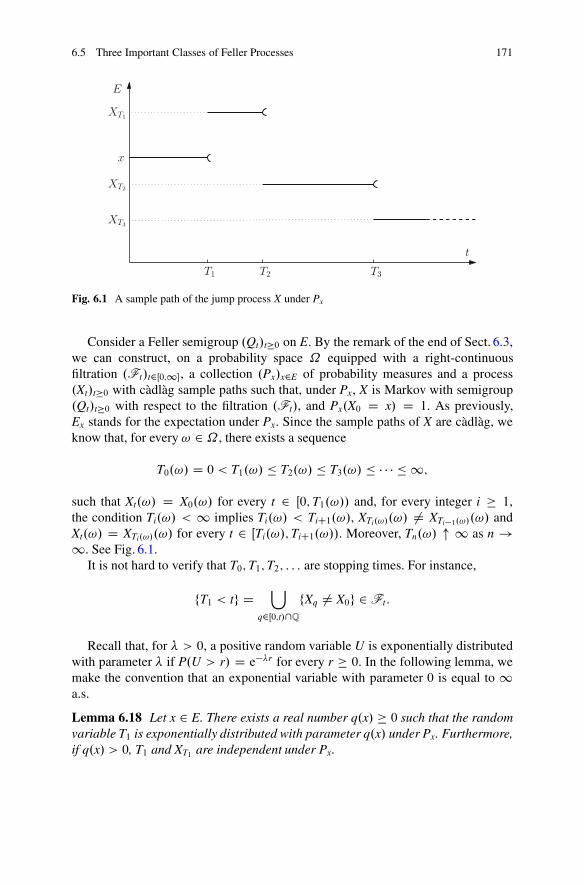
6.5 Three Important Classes of Feller Processes 171

x

XT1

XT2

XT3

t

E

T1 T2 T3

Fig. 6.1 A sample path of the jump process X under Px

Consider a Feller semigroup .Qt/t�0 on E. By the remark of the end of Sect. 6.3,we can construct, on a probability space ˝ equipped with a right-continuousfiltration .Ft/t2Œ0;1�, a collection .Px/x2E of probability measures and a process.Xt/t�0 with càdlàg sample paths such that, under Px, X is Markov with semigroup.Qt/t�0 with respect to the filtration .Ft/, and Px.X0 D x/ D 1. As previously,Ex stands for the expectation under Px. Since the sample paths of X are càdlàg, weknow that, for every ! 2 ˝ , there exists a sequence

T0.!/ D 0 < T1.!/ � T2.!/ � T3.!/ � � � � � 1;

such that Xt.!/ D X0.!/ for every t 2 Œ0;T1.!// and, for every integer i � 1,the condition Ti.!/ < 1 implies Ti.!/ < TiC1.!/, XTi.!/.!/ 6D XTi�1.!/.!/ andXt.!/ D XTi.!/.!/ for every t 2 ŒTi.!/;TiC1.!//. Moreover, Tn.!/ " 1 as n !1. See Fig. 6.1.

It is not hard to verify that T0;T1;T2; : : : are stopping times. For instance,

fT1 < tg D[

q2Œ0;t/\Q

fXq 6D X0g 2 Ft:

Recall that, for � > 0, a positive random variable U is exponentially distributedwith parameter � if P.U > r/ D e��r for every r � 0. In the following lemma, wemake the convention that an exponential variable with parameter 0 is equal to 1a.s.

Lemma 6.18 Let x 2 E. There exists a real number q.x/ � 0 such that the randomvariable T1 is exponentially distributed with parameter q.x/ under Px. Furthermore,if q.x/ > 0, T1 and XT1 are independent under Px.


Proof Let s; t � 0. We have

Px.T1 > s C t/ D ExŒ1fT1>sg ˚..XsCr/r�0/�;

where ˚.f / D 1ff .r/Df .0/; 8r2Œ0;t�g for f 2 D.E/. Using the simple Markov property(Theorem 6.16), we get

Px.T1 > s C t/ D ExŒ1fT1>sg EXs Œ˚..Xr/r�0��

D ExŒ1fT1>sg Px.T1 > t/�

D Px.T1 > s/Px.T1 > t/;

which implies that T1 is exponentially distributed under Px.Assume that q.x/ > 0, so that T1 < 1, Px a.s. Then, for every t � 0 and y 2 E,

Px.T1 > t; XT1 D y/ D ExŒ1fT1>tg �..XtCr/r�0/�;

where for f 2 D.E/, �.f / D 0 is f is constant, and otherwise �. f / D 1f�1.f /Dyg, if�1.f / is the value of f after its first jump. We thus get

Px.T1 > t; XT1 D y/ D ExŒ1fT1>tg EXt Œ�..Xr/r�0/��

D ExŒ1fT1>tg Px.XT1 D y/�

D Px.T1 > t/Px.XT1 D y/;

which gives the desired independence. utPoints x such that q.x/ D 0 are absorbing states for the Markov process, in the

sense that Px.Xt D x;8t � 0/ D 1.For every x 2 E such that q.x/ > 0, and every y 2 E, we set

˘.x; y/ D Px.XT1 D y/:

Note that ˘.x; �/ is a probability measure on E, and ˘.x; x/ D 0.

Proposition 6.19 Let L denote the generator of .Qt/t�0. Then D.L/ D C0.E/ DB.E/, and, for every ' 2 B.E/, for every x 2 E:

• if q.x/ D 0, L'.x/ D 0;• if q.x/ > 0,

L'.x/ D q.x/X

y2E;y 6Dx

˘.x; y/.'.y/ � '.x// DXy2E

L.x; y/ '.y/;


where

L.x; y/ D�

q.x/˘.x; y/ if y 6D x;�q.x/ if y D x:

Proof Let ' 2 B.E/ and x 2 E. If q.x/ D 0, it is trivial that Qt'.x/ D '.x/ and so

limt#0

Qt'.x/ � '.x/t

D 0:

Suppose then that q.x/ > 0. We first observe that

Px.T2 � t/ D O.t2/ (6.1)

as t ! 0. Indeed, using the strong Markov property at T1,

Px.T2 � t/ � Px.T1 � t; T2 � T1 C t/ D ExŒ1fT1�tg PXT1.T1 � t/�;

and we can bound

PXT1.T1 � t/ � sup

y2EPy.T1 � t/ � t sup

y2Eq.y/;

giving the desired result since we have also Px.T1 � t/ � q.x/t.It follows from (6.1) that

Qt'.x/ D ExŒ'.Xt/� D ExŒ'.Xt/ 1ft<T1g�C ExŒ'.XT1 / 1fT1�tg�C O.t2/

D '.x/ e�q.x/t C .1 � e�q.x/t/X

y2E;y 6Dx

˘.x; y/ '.y/C O.t2/;

using the independence of T1 and XT1 and the definition of ˘.x; y/. We concludethat

Qt'.x/ � '.x/t

�!t!0

�q.x/'.x/C q.x/X

y2E;y 6Dx

˘.x; y/ '.y/;

and this completes the proof. utIn particular, taking '.y/ D 1fyg, we have if y 6D x,

L.x; y/ D d

dtPx.Xt D y/jtD0;

so that L.x; y/ can be interpreted as the instantaneous rate of transition from x to y.


The next proposition provides a complete description of the sample paths of Xunder Px. For the sake of simplicity, we assume that there are no absorbing states,but the reader will easily extend the statement to the general case.

Proposition 6.20 We assume that q.y/ > 0 for every y 2 E. Let x 2 E. Then,Px a.s., the jump times T1 < T2 < T3 < � � � are all finite and the sequenceX0;XT1 ;XT2 ; : : : is under Px a discrete Markov chain with transition kernel˘ startedfrom x. Furthermore, conditionally on .X0;XT1 ;XT2 ; : : :/, the random variablesT1 � T0;T2 � T1; : : : are independent and, for every integer i � 0, the conditionaldistribution of TiC1 � Ti is exponential with parameter q.XTi/.

Proof An application of the strong Markov property shows that all stopping timesT1;T2; : : : are finite Px a.s. Then, let y; z 2 E, and f1; f2 2 B.RC/. By the strongMarkov property at T1,

ExŒ1fXT1Dygf1.T1/ 1fXT2Dzgf2.T2 � T1/�

D ExŒ1fXT1Dygf1.T1/EXT1Œ1fXT1Dzgf2.T1/��

D ˘.x; y/˘.y; z/Z 1

0

ds1 e�q.x/s1 f1.s1/Z 1

0

ds2e�q.y/s2 f2.s2/:

Arguing by induction, we get for every y1; : : : ; yp 2 E and f1; : : : ; fp 2 B.RC/,

ExŒ1fXT1Dy1g1fXT2Dy2g � � � 1fXTp Dypg f1.T1/f2.T2 � T1/ � � � fp.Tp � Tp�1/�

D ˘.x; y1/˘.y1; y2/ � � �˘.yp�1; yp/

pYiD1

� Z 1

0

ds e�q.yi�1/sfi.s/�;

where y0 D x by convention. The various assertions of the proposition follow. utJump processes play an important role in various models of applied probability,

in particular in reliability and in queueing theory. In such applications, one usuallystarts from the transition rates of the process. It is thus important to know whether,given a collection .q.x//x2E of nonnegative real numbers and, for every x suchthat q.x/ > 0, a probability measure ˘.x; �/ on E such that ˘.x; x/ D 0,there exists a corresponding Feller semigroup .Qt/t�0 and therefore an associatedMarkov process. The answer to this question is yes, and one can give two differentarguments:

• Probabilistic method. Use the description of Proposition 6.20 (or its extensionto the case where there are absorbing states) to construct the process .Xt/t�0starting from any x 2 E, and thus the semigroup .Qt/t�0 via the formulaQt'.x/ D ExŒ'.Xt/�.


• Analytic method. Define the generator L via the formulas of Proposition 6.19,and observe that the semigroup .Qt/t�0, if it exists, must solve the differentialequation

d

dtQt.x; y/ D QtL.x; y/

by Proposition 6.11. This leads to

Qt D exp.t L/;

in the sense of the exponential of matrices. Since �Id C L has nonnegativeentries if � > 0 is large enough, one immediately gets that Qt has nonnegativeentries. Writing 1 for the vector .1; 1; : : : ; 1/, the property L1 D 0 givesQt1 D 1, so that .Qt.x; �//x2E defines a transition kernel. Finally, the propertyexp..s C t/ L/ D exp.s L/ exp.t L/ gives the Chapman–Kolmogorov property,and we get that .Qt/t�0 is a transition semigroup on E, whose Feller property isalso immediate.

Many of the preceding results can be extended to Feller Markov processes on acountable state space E. Note, however, that certain difficulties arise in the questionof the existence of a process with given transition rates. In fact, starting from theprobabilistic description of Proposition 6.20, one needs to avoid the possibility ofan accumulation of jumps in a finite time interval, which may occur if the rates.q.y/; y 2 E/ are unbounded – of course this problem does not occur when E isfinite.

6.5.2 Lévy Processes

Consider a real process .Yt/t�0 which satisfies the following three assumptions:

(i) Y0 D 0 a.s.(ii) For every 0 � s � t, the variable Yt � Ys is independent of .Yr; 0 � r � s/ and

has the same law as Yt�s.(iii) Yt converges in probability to 0 when t # 0.

Two special cases are real Brownian motion (started from 0) and the process.Ta/a�0 of hitting times of a real Brownian motion (cf. Exercise 2.26).

Notice that we do not assume that sample paths of Y are càdlàg, but only theweaker regularity assumption (iii). The preceding theory will allow us to find amodification of Y with càdlàg sample paths.

For every t � 0, we denote the law of Yt by Qt.0; dy/, and, for every x 2 R, welet Qt.x; dy/ be the image of Qt.0; dy/ under the translation y 7! x C y.


Proposition 6.21 The collection .Qt/t�0 is a Feller semigroup on R. Furthermore,.Yt/t�0 is a Markov process with semigroup .Qt/t�0.

Proof Let us show that .Qt/t�0 is a transition semigroup. Let ' 2 B.R/, s; t � 0 andx 2 R. Property (ii) shows that the law of .Yt;YtCs � Yt/ is the product probabilitymeasure Qt.0; �/˝ Qs.0; �/. Hence,

ZQt.x; dy/

ZQs.y; dz/'.z/ D

ZQt.0; dy/

ZQs.0; dz/'.x C y C z/

D EŒ'.x C Yt C .YtCs � Yt//�

D EŒ'.x C YtCs/�

DZ

QtCs.x; dz/'.z/

giving the Chapman–Kolmogorov relation. We should also verify the measurabilityof the mapping .t; x/ 7! Qt.x;A/, but this will follow from the stronger continuityproperties that we will establish in order to verify the Feller property.

Let us start with the first property of the definition of a Feller semigroup. If' 2 C0.R/, the mapping

x 7! Qt'.x/ D EŒ'.x C Yt/�

is continuous by dominated convergence, and, again by dominated convergence, wehave

EŒ'.x C Yt/� �!x!1 0

showing that Qt' 2 C0.R/. Then,

Qt'.x/ D EŒ'.x C Yt/� �!t!0

'.x/

thanks to property (iii). The uniform continuity of ' even shows that the latterconvergence is uniform in x. This completes the proof of the first assertion of theproposition. To get the second one, we write, for every s; t � 0 and every ' 2 B.R/,

EŒ'.YsCt/ j Yr; 0 � r � s� D EŒ'.Ys C .YsCt � Ys// j Yr; 0 � r � s�

DZ'.Ys C y/Qt.0; dy/

DZ'.y/Qt.Ys; dy/;

using property (ii) and the definition of Qt.0; �/ in the second equality. ut


It then follows from Theorem 6.15 that there exists a modification of .Yt/t�0 withcàdlàg sample paths. Obviously this modification still satisfies (i) and (ii).

A Lévy process is a process satisfying properties (i) and (ii) above, and havingcàdlàg sample paths (which implies (iii)). We refer to [3] for a thorough account ofthe theory of Lévy processes.

6.5.3 Continuous-State Branching Processes

A Markov process .Xt/t�0 with values in E D RC is called a continuous-statebranching process if its semigroup .Qt/t�0 satisfies the following property: for everyx; y 2 RC and t � 0,

Qt.x; �/ Qt.y; �/ D Qt.x C y; �/;

where denotes the convolution of the probability measures and on RC.Note that this implies Qt.0; �/ D ı0 for every t � 0.

Exercise Verify that, if X and X0 are two independent continuous-state branchingprocesses with the same semigroup .Qt/t�0, then .Xt C X0

t/t�0 is also a Markovprocess with semigroup .Qt/t�0. This is the so-called branching property: comparewith discrete time Galton–Watson processes.

Let us fix the semigroup .Qt/t�0 of a continuous-state branching process, andassume that:

(i) Qt.x; f0g/ < 1 for every x > 0 and t > 0;(ii) Qt.x; �/ �! ıx.�/ when t ! 0, in the sense of weak convergence of probability

measures.

Proposition 6.22 Under the preceding assumptions, the semigroup .Qt/t�0 isFeller. Furthermore, for every � > 0, and every x � 0,

ZQt.x; dy/ e��y D e�x t.�/

where the functions t W .0;1/ �! .0;1/ satisfy t ı s D tCs for every s; t � 0.

Proof Let us start with the second assertion. If x; y > 0, the equality Qt.x; �/ Qt.y; �/ D Qt.x C y; �/ implies that

� ZQt.x; dz/ e��z

�� ZQt.y; dz/ e��z

�DZ

Qt.x C y; dz/ e��z:


Thus the function

x 7! � log� Z

Qt.x; dz/ e��z�

is nondecreasing and linear on RC, hence of the form x t.�/ for some constant t.�/ > 0 (the case t.�/ D 0 is excluded by assumption (i)). To obtain the identity t ı s D tCs, we write

ZQtCs.x; dz/ e��z D

ZQt.x; dy/

ZQs.y; dz/ e��z

DZ

Qt.x; dy/ e�y s.�/

D e�x t. s.�//:

We still have to prove that the semigroup is Feller. For every � > 0, set '�.x/ De��x. Then,

Qt'� D ' t.�/ 2 C0.RC/:

Furthermore, an application of the Stone–Weierstrass theorem shows that the vectorspace generated by the functions '�, � > 0, is dense in C0.RC/. It easily followsthat Qt' 2 C0.RC/ for every ' 2 C0.RC/.

Finally, if ' 2 C0.RC/, for every x � 0,

Qt'.x/ DZ

Qt.x; dy/ '.y/ �!t!0

'.x/

by assumption (ii). Using a remark following the definition of Feller semigroups,this suffices to show that kQt' �'k �! 0 when t ! 0, which completes the proof.

utExample For every t > 0 and every x � 0, define Qt.x; dy/ as the law ofe1 C e2 C � � � C eN , where e1; e2; : : : are independent random variables withexponential distribution of parameter 1=t, and N is Poisson with parameter x=t, andis independent of the sequence .ei/. Then a simple calculation shows that

ZQt.x; dy/ e��y D e�x t.�/

where

t.�/ D �

1C �t:

Exercises 179

Noting that t ı s D tCs, we obtain that .Qt/t�0 satisfies the Chapman–Kolmogorov identity, and then that .Qt/t�0 is the transition semigroup of acontinuous-state branching process. Furthermore, .Qt/t�0 satisfies assumptions (i)and (ii) above. In particular, the semigroup .Qt/t�0 is Feller, and one can constructan associated Markov process .Xt/t�0 with càdlàg sample paths. One can in factprove that the sample paths of .Xt/t�0 are continuous, and this process is calledFeller’s branching diffusion, see Sect. 8.4.3 below.

Exercises

Exercise 6.23 (Reflected Brownian motion) We consider a probability spaceequipped with a filtration .Ft/t2Œ0;1�. Let a � 0 and let B D .Bt/t�0 be an.Ft/-Brownian motion such that B0 D a. For every t > 0 and every z 2 R, we set

pt.z/ D 1p2�t

exp.� z2

2t/:

1. We set Xt D jBtj for every t � 0. Verify that, for every s � 0 and t � 0, for everybounded measurable function f W RC �! R,

EŒf .XsCt/ jFs� D Qtf .Xs/;

where Q0f D f and, for every t > 0, for every x � 0,

Qtf .x/ DZ 1

0

�pt.y � x/C pt.y C x/

�f .y/ dy:

2. Infer that .Qt/t�0 is a transition semigroup, then that .Xt/t�0 is a Markov processwith values in E D RC, with respect to the filtration .Ft/, with semigroup.Qt/t�0.

3. Verify that .Qt/t�0 is a Feller semigroup. We denote its generator by L.4. Let f be a twice continuously differentiable function on RC, such that f and

f 00 belong to C0.RC/. Show that, if f 0.0/ D 0, f belongs to the domain of L,and Lf D 1

2f 00. (Hint: One may observe that the function g W R ! R defined

by g.y/ D f .jyj/ is then twice continuously differentiable on R.) Show that,conversely, if f 0.0/ 6D 0, f does not belong to the domain of L.

Exercise 6.24 Let .Qt/t�0 be a transition semigroup on a measurable space E. Let� be a measurable mapping from E onto another measurable space F. We assumethat, for any measurable subset A of F, for every x; y 2 E such that �.x/ D �.y/,we have

Qt.x; ��1.A// D Qt.y; �

�1.A//;


for every t > 0. We then set, for every z 2 F and every measurable subset A of F,for every t > 0,

Q0t.z;A/ D Qt.x; �

�1.A//

where x is an arbitrary point of E such that �.x/ D z. We also set Q00.z;A/ D 1A.z/.

We assume that the mapping .t; z/ 7! Q0t.z;A/ is measurable on RC � F, for every

fixed A.

1. Verify that .Q0t/t�0 forms a transition semigroup on F.

2. Let .Xt/t�0 be a Markov process in E with transition semigroup .Qt/t�0 withrespect to the filtration .Ft/t�0. Set Yt D �.Xt/ for every t � 0. Verify that.Yt/t�0 is a Markov process in F with transition semigroup .Q0

t/t�0 with respectto the filtration .Ft/t�0.

3. Let .Bt/t�0 be a d-dimensional Brownian motion, and set Rt D jBtj for everyt � 0. Verify that .Rt/t�0 is a Markov process and give a formula for itstransition semigroup. (The case d D 1 was treated via a different approach inExercise 6.23.)

In the remaining exercises, we use the following notation. .E; d/ is a locallycompact metric space, which is countable at infinity, and .Qt/t�0 is a Fellersemigroup on E. We consider an E-valued process .Xt/t�0 with càdlàg sample paths,and a collection .Px/x2E of probability measures on E, such that, under Px, .Xt/t�0is a Markov process with semigroup .Qt/t�0, with respect to the filtration .Ft/, andPx.X0 D x/ D 1. We write L for the generator of the semigroup .Qt/t�0, D.L/ forthe domain of L and R� for the �-resolvent, for every � > 0.

Exercise 6.25 (Scale function) In this exercise, we assume that E D RC and thatthe sample paths of X are continuous. For every x 2 RC, we set

Tx WD infft � 0 W Xt D xg

and

'.x/ WD Px.T0 < 1/:

1. Show that, if 0 � x � y;

'.y/ D '.x/Py.Tx < 1/:

2. We assume that '.x/ < 1 and Px.supt�0 Xt D C1/ D 1, for every x > 0. Showthat, if 0 < x � y;

Px.T0 < Ty/ D '.x/ � '.y/1 � '.y/ :

Exercises 181

Exercise 6.26 (Feynman–Kac formula) Let v be a nonnegative function in C0.E/.For every x 2 E and every t � 0, we set, for every ' 2 B.E/,

Q�t '.x/ D Ex

h'.Xt/ exp

��Z t

0

v.Xs/ ds�i:

1. Show that, for every ' 2 B.E/ and s; t � 0, Q�tCs' D Q�

t .Q�s '/.

2. After observing that

1 � exp�

�Z t

0

v.Xs/ ds�

DZ t

0

v.Xs/ exp�

�Z t

sv.Xr/ dr

�ds

show that, for every ' 2 B.E/,

Qt' � Q�t ' D

Z t

0

Qs.vQ�t�s'/ ds:

3. Assume that ' 2 D.L/. Show that

d

dtQ�

t 'jtD0 D L' � v':

Exercise 6.27 (Quasi left-continuity) Throughout the exercise we fix the startingpoint x 2 E. For every t > 0, we write Xt�.!/ for the left-limit of the sample paths 7! Xs.!/ at t.

Let .Tn/n�1 be a strictly increasing sequence of stopping times, and T D lim "Tn. We assume that there exists a constant C < 1 such that T � C. The goal of theexercise is to verify that XT� D XT , Px a.s.

1. Let f 2 D.L/ and h D Lf . Show that, for every n � 1,

ExŒf .XT / j FTn � D f .XTn/C Ex

h Z T

Tn

h.Xs/ dsˇ̌ˇFTn

i:

2. We recall from the theory of discrete time martingales that

ExŒf .XT/ j FTn �a:s:; L1�!n!1 ExŒf .XT/ j eF T �

where

eF T D1_

nD1FTn :


Infer from question (1) that

ExŒf .XT / j eF T � D f .XT�/:

3. Show that the conclusion of question (2) remains valid if we only assume thatf 2 C0.E/, and infer that, for every choice of f ; g 2 C0.E/,

ExŒf .XT /g.XT�/� D ExŒf .XT�/g.XT�/�:

Conclude that XT� D XT , Px a.s.

Exercise 6.28 (Killing operation) In this exercise, we assume that X has continuoussample paths. Let A be a compact subset of E and

TA D infft � 0 W Xt 2 Ag:

1. We set, for every t � 0 and every bounded measurable function ' on E,

Q�t '.x/ D ExŒ'.Xt/ 1ft<TAg� ; 8x 2 E:

Verify that Q�tCs' D Q�

t .Q�s '/, for every s; t > 0.

2. We set E D .EnA/[ f�g, where � is a point added to EnA as an isolated point.For every bounded measurable function ' on E and every t � 0, we set

Qt'.x/ D ExŒ'.Xt/ 1ft<TAg�C PxŒTA � t� '.�/ ; if x 2 EnA

and Qt'.�/ D '.�/. Verify that .Qt/t�0 is a transition semigroup on E. (Theproof of the measurability of the mapping .t; x/ 7! Qt'.x/ will be omitted.)

3. Show that, under the probability measure Px, the process X defined by

Xt D�

Xt if t < TA

� if t � TA

is a Markov process with semigroup .Qt/t�0, with respect to the canonicalfiltration of X.

4. We take it for granted that the semigroup .Qt/t�0 is Feller, and we denote itsgenerator by L. Let f 2 D.L/ such that f and Lf vanish on an open set containingA. Write f for the restriction of f to EnA, and consider f as a function on E bysetting f .�/ D 0. Show that f 2 D.L/ and L f .x/ D Lf .x/ for every x 2 EnA.

Exercise 6.29 (Dynkin’s formula)

1. Let g 2 C0.E/ and x 2 E, and let T be a stopping time. Justify the equality

Ex

h1fT<1ge��T

Z 1

0

e��tg.XTCt/ dti

D ExŒ1fT<1g e��T R�g.XT/�:


2. Infer that

R�g.x/ D Ex

h Z T

0

e��tg.Xt/ dti

C ExŒ1fT<1g e��T R�g.XT/�:

3. Show that, if f 2 D.L/,

f .x/ D Ex

h Z T

0

e��t.�f � Lf /.Xt/ dti

C ExŒ1fT<1g e��T f .XT/�:

4. Assuming that ExŒT� < 1, infer from the previous question that

Ex

h Z T

0

Lf .Xt/ dti

D ExŒf .XT /�� f .x/:

How could this formula have been established more directly?5. For every " > 0, we set T";x D infft � 0 W d.x;Xt/ > "g. Assume that ExŒT";x� <

1, for every sufficiently small ". Show that (still under the assumption f 2 D.L/)one has

Lf .x/ D lim"#0

ExŒf .XT";x/� � f .x/

ExŒT";x�:

6. Show that the assumption ExŒT";x� < 1 for every sufficiently small " holds if thepoint x is not absorbing, that is, if there exists a t > 0 such that Qt.x; fxg/ < 1.(Hint: Observe that there exists a nonnegative function h 2 C0.E/which vanisheson a ball centered at x and is such that Qth.x/ > 0. Infer that one can choose˛ > 0 and � 2 .0; 1/ such that Px.T˛;x > nt/ � .1� �/n for every integer n � 1.)

Notes and Comments

The theory of Markov processes is a very important area of probability theory.Markov processes have a long history that would be too long to summarize here.Dynkin and Feller played a major role in the development of the theory (seein particular Dynkin’s books [20, 21]). We limited our treatment to the minimalmaterial needed for our later applications to stochastic differential equations. Ourtreatment of Feller processes is inspired by the corresponding chapters in [70] and[71]. We chose to focus on Feller semigroups because this special case allowsan easy presentation of key notions such as the generator, and at the same timeit includes the main examples we consider in this book. The reader interested inthe more general theory of Markov processes may have a look at the classicalbooks of Blumenthal and Getoor [5], Meyer [59] and Sharpe [73]. The idea ofcharacterizing a Markov process by a collection of associated martingales (in the


spirit of Theorem 6.14) has led to the theory of martingale problems, for whichwe refer the reader to the classical book of Stroock and Varadhan [77]. Martingaleproblems are also discussed in the book [24] of Ethier and Kurtz, which focuseson problems of characterization and convergence of Markov processes, with manyexamples and applications. Markov processes with a countable state space aretreated, along with other topics, in the more recent book [76] of Stroock. We referto the monograph [3] of Bertoin for a modern presentation of the theory of Lévyprocesses.

Chapter 7Brownian Motion and Partial DifferentialEquations

In this chapter, we use the results of the preceding two chapters to discussconnections between Brownian motion and partial differential equations. After abrief discussion of the heat equation, we focus on the Laplace equation�u D 0 andon the relations between Brownian motion and harmonic functions on a domain ofR

d. In particular, we give the probabilistic solution of the classical Dirichlet problemin a bounded domain whose boundary satisfies the exterior cone condition. In thecase where the domain is a ball, the solution is made explicit by the Poisson kernel,which corresponds to the density of the exit distribution of the ball for Brownianmotion. We then discuss recurrence and transience of d-dimensional Brownianmotion, and we establish the conformal invariance of planar Brownian motion as asimple corollary of the results of Chap. 5. An important application is the so-calledskew-product decomposition of planar Brownian motion, which we use to deriveseveral asymptotic laws, including the celebrated Spitzer theorem on Brownianwindings.

7.1 Brownian Motion and the Heat Equation

Throughout this chapter, we let B stand for a d-dimensional Brownian motion thatstarts from x under the probability measure Px, for every x 2 R

d (one may usethe canonical construction of Sect. 2.2, defining Px as the image of Wiener measureW.dw/ under the translation w 7! x C w). Then .Bt/t�0 is a Feller process withsemigroup

Qt'.x/ DZRd.2�t/�d=2 exp.�jy � xj2

2t/ '.y/ dy;


185

186 7 Brownian Motion and Partial Differential Equations

for ' 2 B.Rd/. We write L for the generator of this Feller process. If is a twicecontinuously differentiable function on R

d such that both and � belong toC0.Rd/, then 2 D.L/ and L D 1

2� (see the end of Sect. 6.2).

If ' 2 B.Rd/, then, for every fixed t > 0, Qt' can be viewed as the convolutionof ' with the C1 function

pt.x/ D .2�t/�d=2 exp.�jxj22t/:

It follows that Qt' is also a C1 function. Furthermore, if ' 2 C0.Rd/, differentia-tion under the integral sign shows that all derivatives of Qt' also belong to C0.Rd/.It follows that we have Qt' 2 D.L/ and L.Qt'/ D 1

2�.Qt'/, for every t > 0.

Theorem 7.1 Let ' 2 C0.Rd/. For every t > 0 and x 2 Rd, set

ut.x/ D Qt'.x/ D ExŒ'.Bt/�:

Then, the function .ut.x//t>0;x2Rd solves the partial differential equation

@ut

@tD 1

2�ut;

on .0;1/� Rd. Furthermore, for every x 2 R

d,

lims#0y!x

us.y/ D '.x/:

Proof By the remarks preceding the theorem, we already know that, for everyt > 0, ut is a C1 function, ut 2 D.L/, and Lut D 1

2�ut. Let " > 0. By applying

Proposition 6.11 to f D u", we get for every t � ",

ut D u" CZ t�"

0

L.Qsu"/ ds D u" CZ t

"

Lus ds:

Since Lus D Qs�".Lu"/ depends continuously on s 2 Œ";1/, it follows that, fort � ",

@ut

@tD Lut D 1

2�ut:

The last assertion is just the fact that Qs' �! ' as s ! 0. utRemark We could have proved Theorem 7.1 by direct calculations from the explicitform of Qt', and these calculations imply that the same statement holds if weonly assume that ' is bounded and continuous. The above proof however has theadvantage of showing the relation between this result and our general study of

7.2 Brownian Motion and Harmonic Functions 187

Markov processes. It also indicates that similar results will hold for more generalequations of the form @u

@t D Au provided A can be interpreted as the generator of anappropriate Markov process.

Brownian motion can be used to provide probabilistic representations for solu-tions of many other parabolic partial differential equations. In particular, solutionsof equations of the form

@u

@tD 1

2�u � v u;

where v is a nonnegative function on Rd, are expressed via the so-called Feynman–

Kac formula: See Exercise 7.28 below for a precise statement.

7.2 Brownian Motion and Harmonic Functions

Let us now turn to connections between Brownian motion and the Laplace equation�u D 0. We start with a classical definition.

Definition 7.2 Let D be a domain of Rd. A function u W D �! R is said to beharmonic on D if it is twice continuously differentiable and �u D 0 on D.

Let D0 be a subdomain of D whose closure is contained in D. Consider thestopping time T WD infft � 0 W Bt … D0g. An application of Itô’s formula (justifiedby the remark preceding Proposition 5.11) shows that, if u is harmonic on D, thenfor every x 2 D0, the process

u.Bt^T/ D u.B0/CZ t^T

0

ru.Bs/ � dBs (7.1)

is a local martingale under Px [here and later, to apply the stochastic calculus resultsof Chap. 5, we let .Ft/ be the canonical filtration of B completed under Px].

So, roughly speaking, harmonic functions are functions which when composedwith Brownian motion give (local) martingales.

Proposition 7.3 Let u be harmonic on the domain D. Let D0 be a boundedsubdomain of D whose closure is contained in D, and consider the stopping timeT WD infft � 0 W Bt … D0g. Then, for every x 2 D0,

u.x/ D ExŒu.BT/�:

Proof Since D0 is bounded, both u and ru are bounded on D0, and we also knowthat Px.T < 1/ D 1 for every x 2 D0. It follows from (7.1) that u.Bt^T/ is a (true)martingale, and in particular, we have

u.x/ D ExŒu.Bt^T/�


for every x 2 D0. By letting t ! 1 and using dominated convergence we get that

u.x/ D ExŒu.BT/�

for every x 2 D0. utThe preceding proposition easily leads to the mean value property for harmonic

functions. In order to state this property, first recall that the uniform probabilitymeasure on the unit sphere, denoted by �1.dy/, is the unique probability measure onfy 2 R

d W jyj D 1g that is invariant under all vector isometries. For every x 2 Rd and

r > 0, we then let �x;r.dy/ be the image of �1.dy/ under the mapping y 7! x C ry.

Proposition 7.4 (Mean value property) Suppose that u is harmonic on thedomain D. Then, for every x 2 D and for every r > 0 such that the closed ballof radius r centered at x is contained in D, we have

u.x/ DZ�x;r.dy/ u.y/:

Proof First observe that, if T1 D infft � 0 W jBtj D 1g, the distribution of BT1under P0 is invariant under all vector isometries of Rd (by the invariance propertiesof Brownian motion stated at the end of Chap. 2) and therefore this distribution is�1.dy/. By scaling and translation invariance, it follows that for every x 2 R

d andr > 0, if Tx;r D infft � 0 W jBt � xj D rg, the distribution of BTx;r under Px is �x;r .However, Proposition 7.3 implies that, under the conditions in the proposition, wemust have u.x/ D ExŒu.BTx;r/�. The desired result follows. ut

We say that a (locally bounded and measurable) function u on D satisfies themean value property if the conclusion of Proposition 7.4 holds. It turns out that thisproperty characterizes harmonic functions.

Lemma 7.5 Let u be a locally bounded and measurable function on D that satisfiesthe mean value property. Then u is harmonic on D.

Proof Fix r0 > 0 and let D0 be the open subset of D consisting of all points whosedistance to Dc is greater than r0. It is enough to prove that u is twice continuouslydifferentiable and�u D 0 on D0. Let h W R �! RC be a C1 function with compactsupport contained in .0; r0/ and not identically zero. Then, for every x 2 D0 andevery r 2 .0; r0/, we have

u.x/ DZ�x;r.dy/ u.y/:

We multiply both sides of this equality by rd�1h.r/ and integrate with respectto Lebesgue measure dr on .0; r0/. Using the formula for integration in polarcoordinates, and agreeing for definiteness that u D 0 on Dc, we get, for every x 2 D0,

c u.x/ DZ

fjyj<r0gdy h.jyj/ u.x C y/ D

ZRd

dz h.jz � xj/ u.z/;


where c > 0 is a constant and we use the fact that h.jz � xj/ D 0 if jz � xj � r0.Since z 7! h.jzj/ is a C1 function, the convolution in the right-hand side of the lastdisplay also defines a C1 function on D0.

It remains to check that �u D 0 on D0. To this end, we use a probabilisticargument (an analytic argument is also easy). By applying Itô’s formula to u.Bt/

under Px, we get, for x 2 D0 and r 2 .0; r0/,

ExŒu.Bt^Tx;r /� D u.x/C Ex

h Z t^Tx;r

0

ds�u.Bs/i:

If we let t ! 1, noting that ExŒTx;r� < 1 (cf. example (b) after Corollary 3.24),we get

ExŒu.BTx;r /� D u.x/C Ex

h Z Tx;r

0

ds�u.Bs/i:

The mean value property just says that ExŒu.BTx;r /� D u.x/ and so we have

Ex

h Z Tx;r

0

ds�u.Bs/i

D 0:

Since this holds for any r 2 .0; r0/ it follows that �u.x/ D 0. utFrom now on, we assume that the domain D is bounded.

Definition 7.6 (Classical Dirichlet problem) Let g be a continuous function on@D. A function u W D �! R solves the Dirichlet problem in D with boundarycondition g, if u is harmonic on D and has boundary condition g, in the sense that,for every y 2 @D, u.x/ �! g.y/ as x ! y, x 2 D.

Recall that ND stands for the closure of D. If u solves the Dirichlet problem withboundary condition g, the function Qu defined on ND by Qu.x/ D u.x/ if x 2 D, andQu.x/ D g.x/ if x 2 @D, is then continuous, hence bounded on ND.

Proposition 7.7 Let D be a bounded domain, and write T D infft � 0 W Bt … Dgfor the exit time of Brownian motion from D.

(i) Let g be a continuous function on @D, and let u be a solution of the Dirichletproblem in D with boundary condition g. Then, for every x 2 D,

u.x/ D ExŒg.BT/�:

(ii) Let g be a bounded measurable function on @D. Then the function

u.x/ D ExŒg.BT/�; x 2 D;

is harmonic on D.


Remark Assertion (i) implies that, if a solution to the Dirichlet problem withboundary condition g exists, then it is unique, which is also easy to prove usingthe mean value property.

Proof

(i) Fix x 2 D and "0 > 0 such that the ball of radius "0 centered at x is containedin D. For every " 2 .0; "0/, let D" be the connected component containing x ofthe open set consisting of all points of D whose distance to Dc is greater than ".If T" D infft � 0 W Bt … D"g, Proposition 7.3 shows that

u.x/ D ExŒu.BT" /�:

Now observe that T" " T as " # 0 (if T 0 is the increasing limit of T" as " # 0,we have T 0 � T and on the other hand BT0 2 @D by the continuity of samplepaths). Using dominated convergence, it follows that ExŒu.BT" /� converges toExŒg.BT/� as " ! 0.

(ii) By Lemma 7.5, it is enough to verify that the function u.x/ D ExŒg.BT/� satisfiesthe mean value property. Recall the notation Tx;r D infft � 0 W jBt � xj D rgfor x 2 R

d and r > 0. Fix x 2 D and r > 0 such that the closed ball of radiusr centered at x is contained in D. We apply the strong Markov property in theform given in Theorem 6.17: With the notation of this theorem, we let˚.w/, forw 2 C.RC;Rd/ such that w.0/ 2 D, be the value of g at the first exit point ofw from D (we take ˚.w/ D 0 if w never exits D) and we observe that we have

g.BT/ D ˚.Bt; t � 0/ D ˚.BTx;rCt; t � 0/; Px a.s.

because the paths .Bt; t � 0/ and .BTx;rCt; t � 0/ have the same exit pointfrom D. It follows that

u.x/ D ExŒg.BT/� D ExŒ˚.BTx;rCt; t � 0/� D ExŒEBT";rŒ˚.Bt; t � 0/�� D ExŒu.BT";r /�:

Since we know that the law of BT";r under Px is �x;r , this gives the mean valueproperty. ut

Part (i) of Proposition 7.7 tells us that the solution of the Dirichlet problem withboundary condition g, if it exists, is given by the probabilistic formula u.x/ DExŒg.BT/�. On the other hand, for any choice of the (bounded measurable) functiong on @D, part (ii) tells us that the probabilistic formula yields a function u that isharmonic on D. Even if g is assumed to be continuous, it is however not clear thatthe function u has boundary condition g, and this need not be true in general (seeExercises 7.24 and 7.25 for examples where the Dirichlet problem has no solution).We state a theorem that gives a partial answer to this question.

If y 2 @D, we say that D satisfies the exterior cone condition at y if there exista (nonempty) open cone C with apex y and a real r > 0 such that the intersectionof C with the open ball of radius r centered at y is contained in Dc. For instance,a convex domain satisfies the exterior cone condition at every point of its boundary.


Theorem 7.8 (Solution of the Dirichlet problem) Let D be a bounded domainin R

d. Assume that D satisfies the exterior cone condition at every y 2 @D. Then,for every continuous function g on @D, the formula

u.x/ D ExŒg.BT/� ; where T D infft � 0 W Bt … Dg;

gives the unique solution of the Dirichlet problem with boundary condition g.

Proof Thanks to Proposition 7.7 (ii), we only need to verify that, for every fixedy 2 @D,

limx!y;x2D

u.x/ D g.y/: (7.2)

Let " > 0. Since g is continuous, we can find ı > 0 such that we have jg.z/�g.y/j �"=3 whenever z 2 @D and jz � yj < ı. Let M > 0 be such that jg.z/j � M for everyz 2 @D. Then, for every � > 0,

ju.x/� g.y/j � ExŒjg.BT/� g.y/j1fT��g�C ExŒjg.BT/� g.y/j1fT>�g�

� ExŒjg.BT/� g.y/j1fT��g1fsupfjBt�xjWt��g�ı=2g�

C2M Px

�supt��

jBt � xj > ı

2

�C 2M Px.T > �/:

Write A1;A2;A3 for the three terms in the sum in the right-hand side of the lastdisplay. We assume that jy�xj < ı=2, and we bound successively these three terms.

First note that we have jBT � yj � jBT � xj C jy � xj < ı on the event

fT � �g \ supfjBt � xj W t � �g � ı=2g;

and our choice of ı ensures that A1 � "=3.Then, translation invariance gives

A2 D 2M P0�

supt��

jBtj > ı

2

�;

which tends to 0 when � > 0 by the continuity of sample paths. So we can fix � > 0so that A2 < "=3.

Finally, we claim that we can choose ˛ 2 .0; ı=2� small enough so that wealso have A3 D 2M Px.T > �/ < "=3 whenever jx � yj < ˛. It follows thatju.x/� g.y/j < ", whenever jx � yj < ˛, thus completing the proof of (7.2). Thus itonly remains to prove our claim, which is the goal of the next lemma. utLemma 7.9 Under the exterior cone condition, we have for every y 2 @D and every� > 0,

limx!y;x2D

Px.T > �/ D 0:


Proof For every u 2 Rd with juj D 1 and every � 2 .0; 1/, consider the circular

cone

C .u; �/ WD fz 2 Rd W z � u > .1 � �/jzjg;

where z � u stands for the usual scalar product. If y 2 @D is given, the exterior conecondition means that we can fix r > 0, u and � such that

y C .C .u; �/\ Br/ � Dc;

where Br denotes the open ball of radius r centered at 0. To simplify notation, weset C D C .u; �/\ Br , and also

C 0 D C .u;�

2/\ Br=2

which is the intersection of a smaller cone with Br=2.For every open subset F of Rd, write TF D infft � 0 W Bt 2 Fg. An application

of Blumenthal’s zero-one law (Theorem 2.13, or rather its easy extension tod-dimensional Brownian motion) along the lines of the proof of Proposition 2.14 (i)shows that P0.TC .u;�=2/ D 0/ D 1 and hence P0.TC 0 D 0/ D 1 by the continuity ofsample paths. On the other hand, set C 0

a D fz 2 C 0 W jzj > ag, for every a 2 .0; r=2/.The sets C 0

a increase to C 0 as a # 0, and thus we have TC 0

a# TC 0 D 0 as a # 0, P0

a.s. Hence, given any ˇ > 0 we can fix a small enough so that

P0.TC 0

a� �/ � 1 � ˇ:

Recalling that y C C � Dc, we have

Px.T � �/ � Px.TyCC � �/ D P0.Ty�xCC � �/:

However, a simple geometric argument shows that, as soon as jy�xj is small enough,the shifted cone y � x C C contains C 0

a , and therefore

Px.T � �/ � P0.TC 0

a� �/ � 1 � ˇ:

Since ˇ was arbitrary, this completes the proof. utRemark The exterior cone condition is only a sufficient condition for the existence(and uniqueness) of a solution to the Dirichlet problem. See e.g. [69] for necessaryand sufficient conditions that ensure the existence of a solution for any continuousboundary value.

7.3 Harmonic Functions in a Ball and the Poisson Kernel 193

7.3 Harmonic Functions in a Ball and the Poisson Kernel

Consider again a bounded domain D and a continuous function g on @D. Let T Dinfft � 0 W Bt … Dg be the exit time of D by Brownian motion. Proposition 7.7 (i)shows that the solution of the Dirichlet problem in D with boundary condition g, ifit exists (which is the case under the assumption of Theorem 7.8), is given by

u.x/ D ExŒg.BT/� DZ@D!.x; dy/ g.y/;

where, for every x 2 D, !.x; dy/ denotes the distribution of BT under Px. Themeasure !.x; dy/ is a probability measure on @D called the harmonic measure ofD relative to x. In general, it is hopeless to try to find an explicit expression for themeasures !.x; dy/. It turns out that, in the case of balls, such an explicit expressionis available and makes the representation of solutions of the Dirichet problem moreconcrete.

From now on, we suppose that D D B1 is the open unit ball in Rd. We also

assume that d � 2 to avoid trivialities. The boundary @B1 is the unit sphere in Rd.

Definition 7.10 The Poisson kernel (of the unit ball) is the function K defined onB1 � @B1 by

K.x; y/ D 1 � jxj2jy � xjd

;

for every x 2 B1 and y 2 @B1.

Lemma 7.11 For every fixed y 2 @B1, the function x 7! K.x; y/ is harmonicon B1.

Proof Set Ky.x/ D K.x; y/ for x 2 B1. Then Ky is a C1 function on B1. Moreovera (somewhat tedious) direct calculation left to the reader shows that �Ky D 0

on B1. utIn view of deriving further properties of the Poisson kernel, the following lemma

about radial harmonic functions will be useful.

Lemma 7.12 Let 0 � r1 < r2 be two real numbers and let h W .r1; r2/ ! R

be a measurable function. The function u.x/ D h.jxj/ is harmonic on the domainfx 2 R

d W r1 < jxj < r2g if and only if there exist two constants a and b such that

h.r/ D�

a C b log r if d D 2;

a C b r2�d if d � 3:

Proof Suppose that u.x/ D h.jxj/ is harmonic on fx 2 Rd W r1 < jxj < r2g.

Then u is twice continuously differentiable and so is h. From the expression of the


Laplacian of a radial function, we get that �u D 0 if and only if

h00.r/C d � 1r

h0.r/ D 0 ; r 2 .r1; r2/:

The solutions of this second order linear differential equations are the functions ofthe form given in the statement. The lemma follows. ut

Recall our notation �1.dy/ for the uniform probability measure on the unitsphere @B1.

Lemma 7.13 For every x 2 B1,

Z@B1

K.x; y/ �1.dy/ D 1:

Proof For every x 2 B1, set

F.x/ DZ@B1

K.x; y/ �1.dy/:

Then the preceding lemma implies that F is harmonic on B1. Indeed, if x 2 B1 andr < 1�jxj, Lemma 7.11 and the mean value property imply that, for every y 2 @B1,

K.x; y/ DZ

K.z; y/ �x;r.dz/:

Hence, using Fubini’s theorem,

ZF.z/ �x;r.dz/ D

Z � ZK.z; y/ �1.dy/

��x;r.dz/

DZ � Z

K.z; y/ �x;r.dz/��1.dy/ D

ZK.x; y/ �1.dy/ D F.x/;

showing that the mean value property holds for F.If is a vector isometry of R

d, we have K. .x/; .y// D K.x; y/ for everyx 2 B1 and y 2 @B1, and the fact that �1.dy/ is invariant under implies thatF. .x// D F.x/ for every x 2 B1. Hence F is a radial harmonic function andLemma 7.12 (together with the fact that F is bounded in the neighborhood of 0)implies that F is constant. Since F.0/ D 1, the proof is complete. utTheorem 7.14 Let g be a continuous function on @B1. The unique solution of theDirichlet problem in B1 with boundary condition g is given by

u.x/ DZ@B1

g.y/K.x; y/ �1.dy/ ; x 2 B1:

7.3 Harmonic Functions in a Ball and the Poisson Kernel 195

Proof The very same arguments as in the beginning of the proof of Lemma 7.13show that u is harmonic on B1. To verify the boundary condition, fix y0 2 @B1.For every ı > 0, the explicit form of the Poisson kernel shows that, if x 2 B1 andy 2 @B1 are such that jx � y0j < ı=2 and jy � y0j > ı, then

K.x; y/ � .2

ı/d .1 � jxj2/:

It follows from this bound that, for every ı > 0,

limx!y0;x2B1

Zfjy�y0j>ıg

K.x; y/ �1.dy/ D 0: (7.3)

Then, given " > 0, we can choose ı > 0 sufficiently small so that the conditionsy 2 @B1 and jy � y0j � ı imply jg.y/ � g.y0/j � ". If M D supfjg.y/j W y 2 @B1g,it follows that

ju.x/� g.y0/j Dˇ̌ˇZ

K.x; y/ .g.y/� g.y0// �1.dy/ˇ̌ˇ

� 2MZ

fjy�y0j>ıgK.x; y/ �1.dy/C ";

using Lemma 7.13 in the first equality, and then our choice of ı. Thanks to (7.3), wenow get

lim supx!y0;x2B1

ju.x/� g.y0/j � ":

Since " was arbitrary, this yields the desired boundary condition. utThe preceding theorem allows us to identify the harmonic measures of the

unit ball.

Corollary 7.15 Let T D infft � 0 W Bt … B1g. For every x 2 B1, the distributionof BT under Px has density K.x; y/ with respect to �1.dy/.

This is immediate since, by combining Proposition 7.7 (i) with Theorem 7.14,we get that, for any continuous function g on @B1,

ExŒg.BT/� DZ@B1

g.y/K.x; y/ �1.dy/ ; 8x 2 B1:


7.4 Transience and Recurrence of Brownian Motion

We consider again a d-dimensional Brownian motion .Bt/t�0 that starts from x underthe probability measure Px. We again suppose that d � 2, since the correspondingresults for d D 1 have already been derived in the previous chapters.

For every a � 0, we introduce the stopping time

Ua D infft � 0 W jBtj D ag;

with the usual convention inf¿ D 1.

Proposition 7.16 Suppose that x 6D 0, and let " and R be such that 0 < " < jxj < R.Then,

Px.U" < UR/ D

8̂ˆ̂<ˆ̂̂:

log R � log jxjlog R � log "

if d D 2;

R2�d � jxj2�d

R2�d � "2�dif d � 3:

(7.4)

Consequently, we have Px.U0 < 1/ D 0 and for every " 2 .0; jxj/,

Px.U" < 1/ D

8̂<:̂1 if d D 2;

� "jxj�d�2

if d � 3:

Proof Write D";R for the annulus fy 2 Rd W " < jyj < Rg. Let u.x/ be the function

defined for x 2 D";R that appears in the right-hand side of (7.4). By Lemma 7.12,u is harmonic on D";R, and it is also clear that u solves the Dirichlet problem inD";R with boundary condition g.y/ D 0 if jyj D R and g.y/ D 1 if jyj D ". IfT";R denotes the first exit time from D";R, Proposition 7.7 shows that we must haveu.x/ D ExŒg.BT";R/� for every x 2 D";R. Formula (7.4) follows since ExŒg.BT";R/� DPx.U" < UR/.

If R > jxj is fixed, the event fU0 < URg is (Px a.s.) contained in fU" < URg, forevery 0 < " < jxj. By passing to the limit " ! 0 in the right-hand side of (7.4),we thus get that Px.U0 < UR/ D 0. Since UR " 1 as R " 1, it follows thatPx.U0 < 1/ D 0.

Finally, we have also Px.U" < 1/ D lim Px.U" < UR/ as R ! 1, andby letting R ! 1 in the right-hand side of (7.4) we get the stated formula forPx.U" < 1/. utRemark The reader will compare formula (7.4) with the exit distribution from aninterval for real Brownian motion that was derived in Chap. 4 (example (a) afterCorollary 3.24). We could have proved (7.4) in a way similar to what we did for

7.4 Transience and Recurrence of Brownian Motion 197

its one-dimensional analog, by applying the optional stopping theorem to the localmartingale log jBtj (if d D 2) or jBtj2�d (if d D 3). See Exercise 5.33.

For every y 2 Rd, set �y D infft � 0 W Bt D yg, so that in particular �0 D U0. The

property Px.�0 < 1/ D 0 for x 6D 0 implies that Px.�y < 1/ D 0 whenever y 6D x,by translation invariance. This means that the probability for Brownian motion tovisit a fixed point other than its starting point is zero: one says that points are polarfor d-dimensional Brownian motion with d � 2 (see Exercise 7.25 for more aboutpolar sets).

If m denotes Lebesgue measure on Rd, it follows from Fubini’s theorem that

ExŒm.fBt; t � 0g/� D Ex

h ZRd

dy 1f�y<1gi

DZRd

dy Px.�y < 1/ D 0;

and therefore m.fBt; t � 0g/ D 0, Px a.s. One can nonetheless prove that theHausdorff dimension of the curve fBt; t � 0g is equal to 2 in any dimension d � 2

(see e.g. [62]). In some sense, this shows that the planar Brownian curve is “not sofar” from having positive Lebesgue measure.

Theorem 7.17

(i) In dimension d D 2, Brownian motion is recurrent, meaning that almost surely,for every nonempty open subset O of Rd, the set ft � 0 W Bt 2 Og is unbounded.

(ii) In dimension d � 3, Brownian motion is transient, meaning that

limt!1 jBtj D 1 ; a.s.

Proof

(i) It is enough to prove that the statement holds when O is an open ball of rationalradius centered at a point with rational coordinates. So it suffices to considera fixed open ball B and we may assume that B is centered at 0 and that thestarting point of B is x 6D 0. By Proposition 7.16 we know that Brownian motionwill never hit 0 (so that inffjBrj W 0 � r � tg > 0 for every t � 0, a.s.) but stillwill hit any open ball centered at 0. It follows that B must visit B at arbitrarilylarge times, a.s.

(ii) Again we can assume that the starting point of B is x 6D 0. Since the functiony 7! jyj2�d is harmonic on R

dnf0g, and since we saw that B does not hit0, we get that jBtj2�d is a local martingale and hence a supermartingale byProposition 4.7. By Theorem 3.19 (and the fact that a positive supermartingaleis automatically bounded in L1), we know that jBtj2�d converges a.s. as t ! 1.The a.s. limit must be zero (otherwise the curve fBt W t � 0g would be bounded!)and this says exactly that jBtj converges to 1 as t ! 1. ut

Remark In dimension d D 2, one can (slightly) reinforce the recurrence propertyby saying that a.s. for every nonempty open subset O of R2, the Lebesgue measureof ft � 0 W Bt 2 Og is infinite. This follows by a straightforward application of thestrong Markov property, and we omit the details.


7.5 Planar Brownian Motion and Holomorphic Functions

In this section, we concentrate on the planar case d D 2, and we write Bt D .Xt;Yt/

for a two-dimensional Brownian motion. It will be convenient to identify R2 with

the complex plane C, so that Bt D Xt C iYt, and we sometimes say that B is acomplex Brownian motion. As previously B starts from z under the probability Pz,for every z 2 C.

If ˚ W C �! C is a holomorphic function, the real and imaginary parts of ˚ areharmonic functions, and thus we know that the real and imaginary parts of ˚.Bt/

are continuous local martingales. In fact, much more is true.

Theorem 7.18 Let˚ W C �! C be a nonconstant holomorphic function. For everyt � 0, set

Ct DZ t

0

j˚ 0.Bs/j2 ds:

Let z 2 C. There exists a complex Brownian motion that starts from ˚.z/ underPz, such that

˚.Bt/ D Ct ; for every t � 0; Pz a.s.

In other words, the image of complex Brownian motion under a holomorphicfunction is a time-changed complex Brownian motion. This is the conformalinvariance property of planar Brownian motion. It is possible (and useful formany applications) to extend Theorem 7.18 to the case where ˚ is defined andholomorphic in a domain D of C (such that z 2 D). A similar representation thenholds for ˚.Bt/ up to the first exit time of D (see e.g. [18]).

Proof Let g and h stand respectively for the real and imaginary parts of ˚ . Since gand h are harmonic, an application of Itô’s formula gives under Pz,

g.Bt/ D g.z/CZ t

0

@g

@x.Bs/ dXs C

Z t

0

@g

@y.Bs/ dYs

and similarly

h.Bt/ D h.z/CZ t

0

@h

@x.Bs/ dXs C

Z t

0

@h

@y.Bs/ dYs:

So Mt D g.Bt/ and Nt D h.Bt/ are local martingales. Moreover, the Cauchy–Riemann equations

@g

@xD @h

@y;@g

@yD �@h

@x

7.5 Planar Brownian Motion and Holomorphic Functions 199

give

hM;Nit D 0

and

hM;Mit D hN;Nit DZ t

0

j˚ 0.Bs/j2 ds D Ct:

The recurrence of planar Brownian motion implies that C1 D 1 a.s. (take a ball Bwhere j˚ 0j is bounded below by a positive constant, and note that the total time spentby B in the ball B is a.s. infinite). We can then apply Proposition 5.15 to Mt � g.z/and Nt � h.z/ under Pz, and we find two independent real Brownian motions ˇ and� started from 0 such that Mt D g.z/ C ˇCt and Nt D h.z/ C �Ct , for every t � 0,a.s. The desired result follows by setting t D ˚.z/C ˇt C i�t. ut

We will apply the conformal invariance property of planar Brownian motionto its decomposition in polar coordinates, which is known as the skew-productrepresentation.

Theorem 7.19 Let z 2 Cnf0g and write z D exp.r C i�/ where r 2 R and � 2.��; ��. There exist two independent linear Brownian motions ˇ and � that startrespectively from r and from � under Pz, such that we have Pz a.s. for every t � 0,

Bt D exp.ˇHt C i �Ht /;

where

Ht DZ t

0

ds

jBsj2 :

Proof The “natural” method for proving Theorem 7.19 would be to apply ageneralized version of Theorem 7.18 to a suitable determination of the complexlogarithm. This, however, leads to some technical difficulties, and for this reason wewill argue differently.

We may assume that z D 1 (and thus r D � D 0). The general case can bereduced to that one using scaling and rotational invariance of Brownian motion. Lett D 1

t C i 2t be a complex Brownian motion started from 0. By Theorem 7.18,

we have a.s. for every t � 0,

exp.t/ D ZCt ; (7.5)

where Z is a complex Brownian motion started from 1, and for every t � 0,

Ct DZ t

0

exp.2 1s / ds:


Let .Hs; s � 0/ be the inverse function of .Ct; t � 0/, so that, by the formula for thederivative of an inverse function,

Hs DZ s

0

exp.�2 1Hu/ du D

Z s

0

du

jZuj2 ;

using the fact that exp. 1Hu/ D jZuj in the last equality. By (7.5) with t D Hs, we

now get

Zs D exp. 1Hs

C i 2Hs/:

This is the desired result (since 1 and 2 are independent linear Brownian motionsstarted from 0) except we did not get it for B but for the complex Brownian motionZ introduced in the course of the argument.

To complete the proof, we argue as follows. Write arg Bt for the continuousdetermination of the argument of Bt such that arg B0 D 0 (this makes sense sincewe know that B does not visit 0, a.s.). The statement of Theorem 7.19 (with z D 1)is equivalent to saying that, if we set

ˇt D log jBinffs�0WR s0 jBuj�2du>tgj;

�t D arg Binffs�0WR s0 jBuj�2du>tg;

then ˇ and � are two independent real Brownian motions started from 0. Note thatˇ and � are deterministic functions of B, and so their law must be the same if wereplace B by the complex Brownian motion Z. This gives the desired result. ut

Let us briefly comment on the skew-product representation. By writing Ht as theinverse of its inverse, we get

Ht D inffs � 0 WZ s

0

exp.2ˇu/ du > tg; (7.6)

and it follows that

log jBtj D ˇinffs�0WR s0 exp.2ˇu/ du>tg;

showing that jBj is completely determined by the linear Brownian motion ˇ. This isrelated to the fact that jBtj is a Markov process, namely a two-dimensional Besselprocess (cf. Exercise 6.24, and Sect. 8.4.3 for a brief discussion of Bessel processes).

On the other hand, write �t D arg Bt D �Ht . Then �t is not a Markov process:At least intuitively, this can be understood by the fact that the past of � up to timet gives information on the current value of jBtj (for instance if �t oscillates veryrapidly just before t this indicates that jBtj should be small) and therefore on thefuture evolution of the process � .

7.6 Asymptotic Laws of Planar Brownian Motion 201

7.6 Asymptotic Laws of Planar Brownian Motion

In this section, we apply the skew-product decomposition to certain asymptoticresults for planar Brownian motion. We fix the starting point z 2 Cnf0g (we willoften take z D 1) and for simplicity we write P instead of Pz. We keep the notation�t D arg Bt for a continuous determination of the argument of Bt. Although theprocess �t is not a Markov process, the fact that it can be written as a linear Brownianmotion time-changed by an independent increasing process allows one to derive alot of information about its path properties. For instance, since Ht �! 1 as t ! 1,we immediately get from Proposition 2.14 that, a.s.,

lim supt!1

�t D C1;

lim inft!1 �t D �1:

One may then ask about the typical size of �t when t is large. This is the celebratedSpitzer theorem on the winding number of planar Brownian motion.

Theorem 7.20 Let .�t; t � 0/ be a continuous determination of the argument of thecomplex Brownian motion B started from z 2 Cnf0g. Then

2

log t�t

converges in distribution as t ! 1 to a standard symmetric Cauchy distribution.In other words, for every x 2 R,

limt!1 P

� 2

log t�t � x

�DZ x

�1dy

�.1C y2/:

Before proving the theorem, we will establish a key lemma. Without loss ofgenerality, we may assume that z D 1 and �0 D 0. We use the notation ofTheorem 7.19, so that ˇ and � are two independent linear Brownian motions startedfrom 0.

Lemma 7.21 For every � > 0, consider the scaled Brownian motion ˇ.�/t D 1�ˇ�2t ,

for every t � 0, and set T.�/1 D infft � 0 W ˇ.�/t D 1g. Then

4

.log t/2Ht � T..log t/=2/

1 �!t!1 0

in probability.

Remark This shows in particular that 4.log t/�2Ht converges in distribution to thelaw of the hitting time of 1 by a linear Brownian motion started from 0.


Proof For every a > 0, set Ta D infft � 0 W ˇt D ag and, for every � > 0,T.�/a D infft � 0 W ˇ.�/t D ag. For the sake of simplicity, we write �t D .log t/=2throughout the proof and always assume that t > 1. We first verify that, for every" > 0,

P�.�t/

�2 Ht > T.�t/1C"�

�!t!1 0: (7.7)

To this end, recall formula (7.6), which shows that

f.�t/�2 Ht > T.�t/

1C"g Dn Z .�t/

2T.�t /1C"

0

exp.2ˇu/ du < to

Dn 12�t

logZ .�t/

2T.�t /1C"

0

exp.2ˇu/ du < 1o; (7.8)

since 2�t D log t. From the change of variables u D .�t/2v in the integral, we get

1

2�tlog

Z .�t/2T.�t /1C"

0

exp.2ˇu/ du D log�t

�tC 1

2�tlog

Z T.�t /1C"

0

exp.2�tˇ.�t/v / dv:

We then note that, for every fixed t > 1, the quantity in the right-hand side has thesame distribution as

log�t

�tC 1

2�tlog

Z T1C"

0

exp.2�tˇv/ dv (7.9)

since for any � > 0 the scaled Brownian motion .ˇ.�/t /t�0 has the same distributionas .ˇt/t�0. We then use the simple analytic fact stating that, for any continuousfunction f W RC �! R, for any s > 0,

1

2�log

Z s

0

exp.2� f .v// dv �!�!1 sup

0�r�sf .r/:

We leave the proof as an exercise for the reader. It follows that

1

2�log

Z T1C"

0

exp.2�ˇv/ dv �!�!1 sup

0�r�T1C"

ˇr D 1C ";

a.s., and so the quantity in (7.9) converges to 1C ", a.s. as t ! 1. Thus,

1

2�tlog

Z .�t/2T.�t /1C"

0

exp.2ˇu/ du �!t!1 1C "

7.6 Asymptotic Laws of Planar Brownian Motion 203

in probability. Hence the probability of the event in the right-hand side of (7.8)tends to 0, proving that (7.7) holds. The very same arguments show that, for every" 2 .0; 1/,

P�.�t/

�2 Ht < T.�t/1�"�

�!t!1 0:

The desired result now follows, noting that T.�t/1�" < T.�t/

1 < T.�t/1C" and that T.�t/

1C"�T.�t/1�"

has the same distribution as T1C"�T1�", which tends to 0 in probability when " ! 0

(clearly, T1�" " T1 as " ! 0, and on the other hand T1C" # T1 a.s. as " ! 0, as aconsequence of the strong Markov property at time T1 and Proposition 2.14 (i)). utProof of Theorem 7.20 We keep the notation introduced in the preceding proofand also consider, for every � > 0, the scaled Brownian motion �.�/t D 1

��2t.

Recalling our notation �t D .log t/=2 for t > 1, we have

2

log t�t D 1

�t�Ht D �

.�t/

.�t/�2Ht:

It then follows from Lemma 7.21 (using also the fact that the linear Brownianmotions �.�/ all have the same distribution) that

2

log t�t � �.�t/

T.�t /1

�!t!1 0;

in probability.To complete the proof, we just have to notice that, for every fixed � > 0, �.�/

T.�/1

has the standard symmetric Cauchy distribution. Indeed, since .ˇ.�/; � .�// is a pairof independent linear Brownian motions started from 0, this variable has the samedistribution as �T1 , and its characteristic distribution is computed by conditioningfirst with respect to T1, and then using the Laplace transform of T1 found in Example(c) after Corollary 3.24,

EŒexp.i��T1 /� D EŒexp.�12�2T1/� D exp.�j�j/;

which we recognize as the characteristic function of the Cauchy distribution. utThe skew-product decomposition and Lemma 7.21 can be used to derive other

asymptotic laws. We know that the planar Brownian motion B started from z 6D0 does not hit 0 a.s., but on the other hand the recurrence property ensures thatminfjBsj W 0 � s � tg tends to 0 as t ! 1. One may then ask about the typical sizeof minfjBsj W 0 � s � tg when t is large: In other words, at which speed does planarBrownian motion approach a point different from its starting point?


Proposition 7.22 Consider the planar Brownian motion B started from z 6D 0.Then, for every a > 0,

limt!1 P

�min0�s�t

jBsj � t�a=2�

D 1

1C a:

For instance, the probability that Brownian motion started from a nonzero initialvalue comes within distance 1=t from the origin before time t converges to 1=3 ast ! 1, a result which was not so easy to guess!

Proof Without loss of generality, we take z D 1. We keep the notation introducedin the proofs of Lemma 7.21 and Theorem 7.20. We observe that

log�

min0�s�t

jBsj�

D min0�s�t

ˇHs D min0�s�Ht

ˇs:

It follows that

2

log tlog

�min0�s�t

jBsj�

D 1

�tmin0�s�Ht

ˇs D min0�s�.�t/�2

ˇ.�t/s :

By Lemma 7.21,

min0�s�.�t/�2

ˇ.�t/s � min

0�s�T.�t /1

ˇ.�t/s �!

t!1 0

in probability. We conclude that we have the following convergence in distribution,

2

log tlog

�min0�s�t

jBsj�

�!t!1 min

0�s�T1ˇs;

where ˇ is a linear Brownian motion started from 0 and T1 D inffs � 0 W ˇs D 1g.To complete the argument, note that

P�

min0�s�T1

ˇs � �a�

D P.T�a < T1/;

if T�a D inffs � 0 W ˇs D �ag, and that P.T�a < T1/ D .1C a/�1 (cf. Sect. 3.4).ut

As a last application of the skew-product decomposition, we state the Kallianpur–Robbins asymptotic law for the time spent by Brownian motion in a ball. Here theinitial value can be arbitrary.

Exercises 205

Theorem 7.23 Let z 2 C and R > 0. Then, under Pz ,

2

log t

Z t

0

1fjBsj<Rg ds

converges in distribution as t ! 1 to an exponential distribution with mean R2.

We postpone our proof of Theorem 7.23 to the end of Chap. 9 since it relies inpart on the theory of local times developed in that chapter.

Exercises

In all exercises, .Bt/t�0 is a d-dimensional Brownian motion starting from x underthe probability measure Px. Except in Exercise 7.28, we always assume that d � 2.

Exercise 7.24 Let B1 be the open unit ball of Rd (d � 2), and B�1 D B1nf0g. Let

g be the continuous function defined on @B�1 by g.x/ D 0 if jxj D 1 and g.0/ D 1.

Prove that the Dirichlet problem in B�1 with boundary condition g has no solution.

Exercise 7.25 (Polar sets) Throughout this exercise, we consider a nonemptycompact subset K of R

d (d � 2). We set TK D infft � 0 W Bt 2 Kg. We saythat K is polar if there exists an x 2 Kc such that Px.TK < 1/ D 0.

1. Using the strong Markov property as in the proof of Proposition 7.7 (ii), provethat the function x 7! Px.TK < 1/ is harmonic on every connected componentof Kc.

2. From now on until question 4., we assume that K is polar. Prove that Kc isconnected, and that the property Px.TK < 1/ D 0 holds for every x 2 Kc.(Hint: Observe that fx 2 Kc W Px.TK < 1/ D 0g is both open and closed).

3. Let D be a bounded domain containing K, and D0 D DnK. Prove that anybounded harmonic function h on D0 can be extended to a harmonic function onD. Does this remain true if the word “bounded” is replaced by “positive”?

4. Set g.x/ D 0 if x 2 @D and g.x/ D 1 if x 2 @D0n@D. Prove that theDirichlet problem in D0 with boundary condition g has no solution. (Note thatthis generalizes the result of Exercise 7.24.)

5. If ˛ 2 .0; d�, we say that the compact set K has zero ˛-dimensional Hausdorffmeasure if, for every " > 0, we can find an integer N" � 1 and N" open ballsB.1/; : : : ;B.N"/ with respective radii r.1/; : : : r.N"/, such that K is contained in theunion B.1/ [ � � � [ B.N"/, and

N"XjD1.rj/

˛ � ":

Prove that if d � 3 and K has zero d � 2-dimensional Hausdorff measure then Kis polar.


Exercise 7.26 In this exercise, d � 3. Let K be a compact subset of the open unitball of Rd, and TK WD infft � 0 W Bt 2 Kg. We assume that D WD R

dnK is connected.We also consider a function g defined and continuous on K. The goal of the exerciseis to determine all functions u W ND ! R that satisfy:

(P) u is bounded and continuous on ND, harmonic on D, and u.y/ D g.y/ if y 2 @D.

(This is the Dirichlet problem in D, but in contrast with Sect. 7.3 above, D isunbounded here.) We fix an increasing sequence .Rn/n�1 of reals, with R1 � 1

and Rn " 1 as n ! 1. For every n � 1, we set T.n/ WD infft � 0 W jBtj � Rng.

1. Suppose that u satisfies (P). Prove that, for every n � 1 and every x 2 D suchthat jxj < Rn,

u.x/ D ExŒg.BTK / 1fTK�T.n/g�C ExŒu.BT.n/ / 1fT.n/�TKg�:

2. Show that, by replacing the sequence .Rn/n�1 with a subsequence if necessary,we may assume that there exists a constant ˛ 2 R such that, for every x 2 D,

limn!1 ExŒu.BT.n/ /� D ˛;

and that we then have

limjxj!1

u.x/ D ˛:

3. Show that, for every x 2 D,

u.x/ D ExŒg.BTK / 1fTK<1g�C ˛ Px.TK D 1/:

4. Assume that D satisfies the exterior cone condition at every y 2 @D (this isdefined in the same way as when D is bounded). Show that, for any choice of˛ 2 R, the formula of question 3. gives a solution of the problem (P).

Exercise 7.27 Let f W C ! C be a nonconstant holomorphic function. Use planarBrownian motion to prove that the set ff .z/ W z 2 Cg is dense in C. (Much more istrue, since Picard’s little theorem asserts that the complement of ff .z/ W z 2 Cg in C

contains at most one point: This can also be proved using Brownian motion, but theargument is more involved, see [12].)

Exercise 7.28 (Feynman–Kac formula for Brownian motion) This is a continua-tion of Exercise 6.26 in Chap. 6. With the notation of this exercise, we assume thatE D R

d and Xt D Bt. Let v be a nonnegative function in C0.Rd/, and assume thatv is continuously differentiable with bounded first derivatives. As in Exercise 6.26,set, for every ' 2 B.Rd/,

Q�t '.x/ D Ex

h'.Xt/ exp

��Z t

0

v.Xs/ ds�i:


1. Using the formula derived in question 2. of Exercise 6.26, prove that, forevery t > 0, and every ' 2 C0.Rd/, the function Q�

t ' is twice continuouslydifferentiable on R

d, and that Q�t ' and its partial derivatives up to order 2 belong

to C0.Rd/. Conclude that Q�t ' 2 D.L/.

2. Let ' 2 C0.Rd/ and set ut.x/ D Q�t '.x/ for every t > 0 and x 2 R

d. Usingquestion 3. of Exercise 6.26, prove that, for every x 2 R

d, the function t 7! ut.x/is continuously differentiable on .0;1/, and

@ut

@tD 1

2�ut � v ut:

Exercise 7.29 In this exercise d D 2 and R2 is identified with the complex plane

C. Let ˛ 2 .0; �/, and consider the open cone

C˛ D fr ei� W r > 0; � 2 .�˛; ˛/g:

Set T WD infft � 0 W Bt … C˛g.

1. Show that the law of log jBT j under P1 is the law of ˇinfft�0Wj�t jD˛g, where ˇ and� are two independent linear Brownian motions started from 0.

2. Verify that, for every � 2 R,

E1Œei� log jBT j� D 1

cosh.˛�/:

Notes and Comments

Connections between Brownian motion and partial differential equations have beenknown for a long time and motivated the study of this random process. A survey ofthe partial differential equations that can be solved in terms of Brownian motion canbe found in the book of Durrett [18, Chapter 8]. The representation of Theorem 7.1(written in terms of the Gaussian density) goes back to the ninetieth century and thework of Fourier and Laplace – see the references in [49]. The beautiful relationsbetween Brownian motion and harmonic functions were discovered and studiedby Kakutani [45, 46], and Hunt [33, 34] later studied the connections betweenpotential theory and transient Markov processes (see the Blumenthal–Getoor book[5] for more on this topic). Nice accounts of the links between Brownian motionand classical potential theory can be found in the books by Port and Stone [69]and Doob [16] (see also Itô and McKean [42], Chung [9], and Chapters 3 and 8 of[62]). The conformal invariance of planar Brownian motion was stated by Lévy [54]with a very sketchy proof. Davis’ paper [12] is a nice survey of relations betweenplanar Brownian motion and analytic functions, see also Durrett’s book [18], and thepaper [28] by Getoor and Sharpe for a notion of conformal martingale that plays inmartingale theory a role similar to that of analytic functions. Spitzer’s theorem was


obtained in the classical paper [75], and the Kallianpur–Robbins law was derived in[48]. A number of remarkable properties of planar Brownian motion had alreadybeen observed by Lévy [53] in 1940. We refer to Pitman and Yor [68] for asystematic study of asymptotic laws of planar Brownian motion. Our presentationclosely follows [52], where other applications of the skew-product decompositioncan be found.

Chapter 8Stochastic Differential Equations

This chapter is devoted to stochastic differential equations, which motivated Itô’sconstruction of stochastic integrals. After giving the general definitions, we providea detailed treatment of the Lipschitz case, where strong existence and uniquenessstatements hold. Still in the Lipschitz case, we show that the solution of a stochasticdifferential equation is a Markov process with a Feller semigroup, whose generatoris a second-order differential operator. By results of Chap. 6, the Feller propertyimmediately gives the strong Markov property of solutions of stochastic differentialequations. The last section presents a few important examples. This chapter can beread independently of Chap. 7.

8.1 Motivation and General Definitions

The goal of stochastic differential equations is to provide a model for a differentialequation perturbed by a random noise. Consider an ordinary differential equation ofthe form

y0.t/ D b.y.t//;

or, in differential form,

dyt D b.yt/ dt:

Such an equation is used to model the evolution of a physical system. If we takerandom perturbations of the system into account, we add a noise term, which istypically of the form � dBt, where B denotes a Brownian motion, and � is a constantcorresponding to the intensity of the noise. Note that the use of Brownian motionhere is justified by its property of independence of increments, corresponding to the


209

210 8 Stochastic Differential Equations

fact that the random perturbations affecting disjoint time intervals are assumed tobe independent.

In this way, we arrive at a stochastic differential equation of the form

dyt D b.yt/ dt C � dBt;

or in integral form, the only one with a rigorous mathematical meaning,

yt D y0 CZ t

0

b.ys/ ds C � Bt:

We generalize the preceding equation by allowing � to depend on the state of thesystem at time t :

dyt D b.yt/ dt C �.yt/ dBt;

or, in integral form,

yt D y0 CZ t

0

b.ys/ ds CZ t

0

�.ys/ dBs:

Because of the integral in dBs, the preceding equation only makes sense thanks tothe theory of stochastic integrals developed in Chap. 5. We can still generalize thepreceding equation by allowing � and b to depend on the time parameter t. Thisleads to the following definition.

Definition 8.1 Let d and m be positive integers, and let � and b be locally boundedmeasurable functions defined on RC � R

d and taking values in Md�m.R/ and in Rd

respectively, where Md�m.R/ is the set of all d � m matrices with real coefficients.We write � D .�ij/1�i�d;1�j�m and b D .bi/1�i�d.

A solution of the stochastic differential equation

E.�; b/ dXt D �.t;Xt/ dBt C b.t;Xt/ dt

consists of:

• a filtered probability space .˝;F ; .Ft/t2Œ0;1�;P/ (where the filtration is alwaysassumed to be complete);

• an m-dimensional .Ft/-Brownian motion B D .B1; : : : ;Bm/ started from 0;• an .Ft/-adapted process X D .X1; : : : ;Xd/ with values in R

d, with continuoussample paths, such that

Xt D X0 CZ t

0

�.s;Xs/ dBs CZ t

0

b.s;Xs/ ds;

8.1 Motivation and General Definitions 211

meaning that, for every i 2 f1; : : : ; dg,

Xit D Xi

0 CmX

jD1

Z t

0

�ij.s;Xs/ dBjs C

Z t

0

bi.s;Xs/ ds:

If additionally X0 D x 2 Rd, we say that X is a solution of Ex.�; b/.

Note that, when we speak about a solution of E.�; b/, we do not fix a priori thefiltered probability space and the Brownian motion B. When we fix these objects,we will say so explicitly.

There are several notions of existence and uniqueness for stochastic differentialequations.

Definition 8.2 For the equation E.�; b/ we say that there is

• weak existence if, for every x 2 Rd, there exists a solution of Ex.�; b/;

• weak existence and weak uniqueness if in addition, for every x 2 Rd, all solutions

of Ex.�; b/ have the same law;• pathwise uniqueness if, whenever the filtered probability space .˝;F ; .Ft/;P/

and the .Ft/-Brownian motion B are fixed, two solutions X and X0 such thatX0 D X0

0 a.s. are indistinguishable.

Furthermore, we say that a solution X of Ex.�; b/ is a strong solution if X is adaptedwith respect to the completed canonical filtration of B.

Remark It may happen that weak existence and weak uniqueness hold but pathwiseuniqueness fails. For a simple example, consider a real Brownian motion ˇ startedfrom ˇ0 D y, and set

Bt DZ t

0

sgn .ˇs/ dˇs;

where sgn .x/ D 1 if x > 0 and sgn .x/ D �1 if x � 0. Then, one immediately getsfrom the “associativity” of stochastic integrals that

ˇt D y CZ t

0

sgn .ˇs/ dBs:

Moreover, B is a continuous martingale with quadratic variation hB;Bit D t, andTheorem 5.12 shows that B is a Brownian motion started from 0. We thus see that ˇsolves the stochastic differential equation

dXt D sgn .Xt/ dBt; X0 D y;

and it follows that weak existence holds for this equation. Theorem 5.12 again showsthat any other solution of this equation must be a Brownian motion, which gives


weak uniqueness. On the other hand, pathwise uniqueness fails. In fact, taking y D 0

in the construction, one easily sees that both ˇ and �ˇ solve the preceding stochasticdifferential equation with the same Brownian motion B and initial value 0 (note thatR t0

1fˇsD0g ds D 0, which impliesR t0

1fˇsD0g dBs D 0). One can also show that ˇ isnot a strong solution: One verifies that the canonical filtration of B coincides withthe canonical filtration of jˇj, which is strictly smaller than that of ˇ (we omit theproof, which is a simple application of formula (9.18) in Chap. 9).

The next theorem links the different notions of existence and uniqueness.

Theorem (Yamada–Watanabe) If both weak existence and pathwise uniquenesshold, then weak uniqueness also holds. Moreover, for any choice of the filteredprobability space .˝;F ; .Ft/;P/ and of the .Ft/-Brownian motion B, there existsfor every x 2 R

d a (unique) strong solution of Ex.�; b/.

We omit the proof (see Yamada and Watanabe [83]) because we will not needthis result. In the Lipschitz case that we will consider, we will establish directly theproperties given by the Yamada–Watanabe theorem.

8.2 The Lipschitz Case

In this section, we work under the following assumptions.

Assumptions The functions � are b are continuous on RC � Rd and Lipschitz in

the variable x: There exists a constant K such that, for every t � 0, x; y 2 Rd,

j�.t; x/ � �.t; y/j � K jx � yj;jb.t; x/� b.t; y/j � K jx � yj:

Theorem 8.3 Under the preceding assumptions, pathwise uniqueness holds forE.�; b/, and, for every choice of the filtered probability space .˝;F ; .Ft/;P/ andof the .Ft/-Brownian motion B, for every x 2 R

d, there exists a (unique) strongsolution of Ex.�; b/.

The theorem implies in particular that weak existence holds for E.�; b/. Weakuniqueness will follow from the next theorem (it can also be deduced from pathwiseuniqueness using the Yamada–Watanabe theorem).

Remark One can “localize” the Lipschitz assumption on � and b, meaning thatthe constant K may depend on the compact set on which the parameters t and x; yare considered. In that case, it is, however, necessary to keep a condition of lineargrowth of the form

j�.t; x/j � K.1C jxj/; jb.t; x/j � K.1C jxj/:

8.2 The Lipschitz Case 213

This kind of condition, which avoids the blow-up of solutions, already appears inordinary differential equations.

Proof For the sake of simplicity, we consider only the case d D m D 1. The readerwill be able to check that the general case follows from exactly the same arguments,at the cost of a heavier notation. Let us start by proving pathwise uniqueness. Weconsider (on the same filtered probability space, with the same Brownian motion B)two solutions X and X0 such that X0 D X0

0. Fix M > 0 and set

� D infft � 0 W jXtj � M or jX0t j � Mg:

Then, for every t � 0,

Xt^� D X0 CZ t^�

0

�.s;Xs/ dBs CZ t^�

0

b.s;Xs/ ds

and an analogous equation holds for X0t^� . Fix a constant T > 0. By considering

the difference between the two equations and using the bound (5.14), we get, fort 2 Œ0;T�,

EŒ.Xt^� � X0

t^� /2�

� 2Eh� Z t^�

0

.�.s;Xs/ � �.s;X0

s// dBs

�2iC 2Eh� Z t^�

0

.b.s;Xs/ � b.s;X0

s// ds�2i

� 2

�Eh Z t^�

0

.�.s;Xs/� �.s;X0

s//2dsi

C T Eh Z t^�

0

.b.s;Xs/ � b.s;X0

s//2dsi�

� 2K2.1C T/Eh Z t^�

0

.Xs � X0

s/2dsi

� 2K2.1C T/Eh Z t

0

.Xs^� � X0

s^� /2dsi:

Hence the function h.t/ D EŒ.Xt^� � X0t^� /2� satisfies

h.t/ � CZ t

0

h.s/ ds

for every t 2 Œ0;T�, with C D 2K2.1C T/.

Lemma 8.4 (Gronwall’s lemma) Let T > 0 and let g be a nonnegative boundedmeasurable function on Œ0;T�. Assume that there exist two constants a � 0 andb � 0 such that, for every t 2 Œ0;T�,

g.t/ � a C bZ t

0

g.s/ ds:


Then, we also have, for every t 2 Œ0;T�,

g.t/ � a exp.bt/:

Proof of the lemma By iterating the condition on g, we get,

g.t/ � a C a.bt/C b2Z t

0

dsZ s

0

dr g.r/

� a C a.bt/C a.bt/2

2C � � � C a

.bt/n

nŠC bnC1

Z t

0

ds1

Z s1

0

ds2 � � �Z sn

0

dsnC1g.snC1/;

for every n � 1. If A is a constant such that 0 � g � A, the last term in the right-hand side is bounded above by A.bt/nC1=.n C 1/Š, hence tends to 0 as n ! 1. Thedesired result now follows. ut

Let us return to the proof of the theorem. The function h is bounded above by4M2 and the assumption of the lemma holds with a D 0, b D C. We thus get h D 0,so that Xt^� D X0

t^� . By letting M tend to 1, we get Xt D X0t , which completes the

proof of pathwise uniqueness.For the second assertion, we construct a solution using Picard’s approximation

method. We define by induction

X0t D x;

X1t D x CZ t

0

�.s; x/ dBs CZ t

0

b.s; x/ ds;

Xnt D x C

Z t

0

�.s;Xn�1s / dBs C

Z t

0

b.s;Xn�1s / ds:

The stochastic integrals are well defined since one verifies by induction that, forevery n, the process Xn is adapted and has continuous sample paths.

It is enough to show that, for every T > 0, there is a strong solution of Ex.�; b/on the time interval Œ0;T�. Indeed, the uniqueness part of the argument will thenallow us to get a (unique) strong solution on RC that will coincide with the solutionon Œ0;T� up to time T.

We fix T > 0 and, for every n � 1 and every t 2 Œ0;T�, we set

gn.t/ D Eh

sup0�s�t

jXns � Xn�1

s j2i:

We will bound the functions gn by induction on n (at present, it is not yet clearthat these functions are finite). The fact that the functions �.�; x/ and b.�; x/ arecontinuous, hence bounded, over Œ0;T� implies that there exists a constant C0

T suchthat g1.t/ � C0

T for every t 2 Œ0;T� (use Doob’s inequality in L2 for the stochasticintegral term).


Then we observe that

XnC1t � Xn

t DZ t

0

.�.s;Xns / � �.s;Xn�1

s // dBs CZ t

0

.b.s;Xns /� b.s;Xn�1

s // ds:

Hence, using the case p D 2 of the Burkholder–Davis–Gundy inequalities in thesecond bound (and writing C.2/ for the constant in this inequality),

Eh

sup0�s�t

jXnC1s � Xn

s j2i

� 2Eh

sup0�s�t

ˇ̌ˇZ s

0

.�.u;Xnu/� �.u;Xn�1

u // dBu

ˇ̌ˇ2

C sup0�s�t

ˇ̌ˇZ s

0

.b.u;Xnu/� b.u;Xn�1

u // duˇ̌ˇ2i

� 2�

C.2/ Eh Z t

0

.�.u;Xnu/ � �.u;Xn�1

u //2 dui

CT Eh Z t

0

.b.u;Xnu/ � b.u;Xn�1

u //2 dui�

� 2.C.2/ C T/K2 Eh Z t

0

jXnu � Xn�1

u j2 dui

� CT Eh Z t

0

sup0�r�u

jXnr � Xn�1

r j2 dui

where CT D 2.C.2/ C T/K2. We have thus obtained that, for every n � 1,

gnC1.t/ � CT

Z t

0

gn.u/ du: (8.1)

Recalling that g1.t/ � C0T , an induction argument using (8.1) shows that, for every

n � 1 and t 2 Œ0;T�,

gn.t/ � C0T .CT/

n�1 tn�1

.n � 1/Š:

In particular,P1

nD1 gn.T/1=2 < 1, which implies that

1XnD0

sup0�t�T

jXnC1t � Xn

t j < 1; a.s.

Hence the sequence .Xnt ; 0 � t � T/ converges uniformly on Œ0;T�, a.s., to a limiting

process .Xt; 0 � t � T/, which has continuous sample paths. By induction, one alsoverifies that, for every n, Xn is adapted with respect to the (completed) canonicalfiltration of B, and the same holds for X.


Finally, from the fact that � and b are Lipschitz in the variable x, we also get that,for every t 2 Œ0;T�,

limn!1

� Z t

0

�.s;Xs/ dBs �Z t

0

�.s;Xns / dBs

�D 0;

limn!1

� Z t

0

b.s;Xs/ ds �Z t

0

b.s;Xns / ds

�D 0;

in probability (to deal with the stochastic integrals, we may use Proposition 5.8,noting that jXn

s � Xsj is dominated byP1

kD0 sup0�r�s jXkC1r � Xk

r j). By passing tothe limit in the induction equation defining Xn, we get that X solves Ex.�; b/ onŒ0;T�. This completes the proof of the theorem. ut

In the following statement, W.dw/ stands for the Wiener measure on thecanonical space C.RC;Rm/ of all continuous functions from RC into R

m (W.dw/is the law of .Bt; t � 0/ if B is an m-dimensional Brownian motion started from 0).

Theorem 8.5 Under the assumptions of the preceding theorem, there exists, forevery x 2 R, a mapping Fx W C.RC;Rm/ �! C.RC;Rd/, which is measurable whenC.RC;Rm/ is equipped with the Borel �-field completed by the W-negligible sets,and C.RC;Rd/ is equipped with the Borel �-field, such that the following propertieshold:

(i) for every t � 0, Fx.w/t coincides W.dw/ a.s. with a measurable function of.w.r/; 0 � r � t/;

(ii) for every w 2 C.RC;Rm/, the mapping x 7! Fx.w/ is continuous;(iii) for every x 2 R

d, for every choice of the (complete) filtered probabilityspace .˝;F ; .Ft/;P/ and of the m-dimensional .Ft/-Brownian motion Bwith B0 D 0, the process Xt defined Xt D Fx.B/t is the unique solution ofEx.�; b/; furthermore, if U is an F0-measurable real random variable, theprocess FU.B/t is the unique solution with X0 D U.

Remark Assertion (iii) implies in particular that weak uniqueness holds forE.�; b/: any solution of Ex.�; b/ must be of the form Fx.B/ and its law is thusuniquely determined as the image of W.dw/ under Fx.

Proof Again we consider only the case d D m D 1. Let N be the class of allW-negligible sets in C.RC;R/, and, for every t 2 Œ0;1�, set

Gt D �.w.s/; 0 � s � t/ _ N :

For every x 2 R, we write Xx for the solution of Ex.�; b/ corresponding to thefiltered probability space .C.RC;R/;G1; .Gt/;W/ and the (canonical) Brownianmotion Bt.w/ D w.t/. This solution exists and is unique (up to indistinguishability)by Theorem 8.3, noting that the filtration .Gt/ is complete by construction.


Let x; y 2 R and let Tn be the stopping time defined by

Tn D infft � 0 W jXxt j � n or jXy

t j � ng:

Let p � 2 and T � 1. Using the Burkholder–Davis–Gundy inequalities (Theo-rem 5.16) and then the Hölder inequality, we get, for t 2 Œ0;T�,

Eh

sups�t

jXxs^Tn

� Xys^Tn

jpi

� Cp

�jx � yjp C E

hsups�t

ˇ̌ˇZ s^Tn

0

.�.r;Xxr /� �.r;Xy

r // dBr

ˇ̌ˇpi

CEh

sups�t

ˇ̌ˇZ s^Tn

0

.b.r;Xxr / � b.r;Xy

r // drˇ̌ˇpi�

� Cp

�jx � yjp C C0

pEh� Z t^Tn

0

.�.r;Xxr /� �.r;Xy

r //2dr�p=2i

CEh� Z t^Tn

0

jb.r;Xxr /� b.r;Xy

r /j dr�pi�

� Cp

�jx � yjp C C0

ptp2�1E

h Z t

0

j�.r ^ Tn;Xxr^Tn

/� �.r ^ Tn;Xyr^Tn

/jpdri

Ctp�1 Eh Z t

0

jb.r ^ Tn;Xxr^Tn

/ � b.r ^ Tn;Xyr^Tn

/jpdri�

� C00p

�jx � yjp C Tp

Z t

0

EŒjXxr^Tn

� Xyr^Tn

jp� dr�;

where the constants Cp;C0p;C

00p < 1 depend on p (and on the constant K appearing

in our assumption on � and b) but not on n or on x; y and T.

As the function t 7! Eh

sups�t jXxs^Tn

� Xys^Tn

jpi

is bounded, Lemma 8.4 implies

that, for t 2 Œ0;T�,

Eh

sups�t

jXxs^Tn

� Xys^Tn

jpi

� C00p jx � yjp exp.C00

p Tpt/;

hence, letting n tend to 1,

Eh

sups�t

jXxs � Xy

s jpi

� C00p jx � yjp exp.C00

p Tpt/:

The topology on the space C.RC;R/ is defined by the distance

d.w;w0/ D1X

kD1˛k

�sups�k

jw.s/� w0.s/j ^ 1�;


where the sequence of positive reals ˛k can be chosen in an arbitrary way, providedthat the series

P˛k converges. We may choose the coefficients ˛k so that

1XkD1

˛k exp.C00p kpC1/ < 1:

For every x 2 R, we consider Xx as a random variable with values in C.RC;R/. Thepreceding estimates and Jensen’s inequality then show that

EŒd.Xx;Xy/p� �� 1X

kD1˛k

�p�1 1XkD1

˛k Eh

sups�k

jXxs � Xy

s jpi

� NCp jx � yjp;

with a constant NCp independent of x and y. By Kolmogorov’s lemma (Theorem 2.9),applied to the process .Xx; x 2 R/ with values in the space E D C.RC;R/ equippedwith the distance d, we get that .Xx; x 2 R/ has a modification with continuoussample paths, which we denote by . QXx; x 2 R/. We set Fx.w/ D QXx.w/ D. QXx

t .w//t�0. Property (ii) is then obvious.The mapping w 7! Fx.w/ is measurable from C.RC;R/ equipped with the �-

field G1 into C.RC;R/ equipped with the Borel �-field C D �.w.s/; s � 0/.Moreover, for every t � 0, Fx.w/t D QXx

t .w/a:s:D Xx

t .w/ is Gt-measurable hence

coincides W.dw/ a.s. with a measurable function of .w.s/; 0 � s � t/. Thusproperty (i) holds.

Let us now prove the first part of assertion (iii). To this end, we fix the filteredprobability space .˝;F ; .Ft/;P/ and the .Ft/-Brownian motion B. We need toverify that the process .Fx.B/t/t�0 then solves Ex.�; b/. This process (trivially) hascontinuous sample paths, and is also adapted since Fx.B/t coincides a.s. with ameasurable function of .Br; 0 � r � t/, by (i), and since the filtration .Ft/ iscomplete. On the other hand, by the construction of Fx (and because QXx D Xx a.s.),we have, for every t � 0, W.dw/ a.s.

Fx.w/t D x CZ t

0

�.s;Fx.w/s/ dw.s/CZ t

0

b.s;Fx.w/s/ds;

where the stochastic integralR t0�.s;Fx.w/s/dw.s/ can be defined by

Z t

0

�.s;Fx.w/s/ dw.s/ D limk!1

2nk �1XiD0

�.it

2nk;Fx.w/it=2nk / .w.

.i C 1/t

2nk/� w.

it

2nk//;


W.dw/ a.s. Here .nk/k�1 is a suitable subsequence, and we used Proposition 5.9. Wecan now replace w by B (whose distribution is W.dw/!) and get a.s.

Fx.B/t D x C limk!1

2nk�1X

iD0

�.it

2nk;Fx.B/it=2nk / .B.iC1/t=2nk � Bit=2nk /C

Z t

0

b.s;Fx.B/s/ds

D x CZ t

0

�.s;Fx.B/s/dBs CZ t

0

b.s;Fx.B/s/ds;

again thanks to Proposition 5.9. We thus obtain that Fx.B/ is the desired solution.We still have to prove the second part of assertion (iii). We again fix the filtered

probability space .˝;F ; .Ft/;P/ and the .Ft/-Brownian motion B. Let U be anF0-measurable random variable. If in the stochastic integral equation satisfied byFx.B/ we formally substitute U for x, we obtain that FU.B/ solves E.�; b/ withinitial value U. However, this formal substitution is not so easy to justify, and wewill argue with some care.

We first observe that the mapping .x; !/ 7! Fx.B/t is continuous with respect tothe variable x (if ! is fixed) and Ft-measurable with respect to ! (if x is fixed). Iteasily follows that this mapping is measurable for the �-field B.R/˝ Ft. Since Uis F0-measurable, we get that FU.B/t is Ft-measurable. Hence the process FU.B/is adapted. For x 2 R and w 2 C.RC;R/, we define G.x;w/ 2 C.RC;R/ by theformula

G.x;w/t DZ t

0

b.s;Fx.w/s/ ds:

We also set H.x;w/ D Fx.w/ � x � G.x;w/. We have already seen that, for everyx 2 R, we have W.dw/ a.s.,

H.x;w/t DZ t

0

�.s;Fx.w/s/ dw.s/:

Hence, if

Hn.x;w/t D2n�1XiD0

�.it

2n;Fx.w/it=2n/ .w.

.i C 1/t

2n/� w.

it

2n//;

Proposition 5.9 shows that

H.x;w/t D limn!1 Hn.x;w/t;

in probability under W.dw/, for every x 2 R. Using the fact that U and B areindependent (because U is F0-measurable), we infer from the latter convergence


that

H.U;B/t D limn!1 Hn.U;B/t

in probability. Thanks again to Proposition 5.9, the limit must be the stochasticintegral

Z t

0

�.s;FU.B/s/ dBs:

We have thus proved that

Z t

0

�.s;FU.B/s/ dBs D H.U;B/t D FU.B/t � U �Z t

0

b.s;FU.B/s/ ds ;

which shows that FU.B/ solves E.�; b/ with initial value U. utA consequence of Theorem 8.5, especially of property (ii) in this theorem, is the

continuity of solutions with respect to the initial value. Given the filtered probabilityspace .˝;F ; .Ft/;P/ and the .Ft/-Brownian motion B, one can construct, forevery x 2 R

d, the solution Xx of Ex.�; b/ in such a way that, for every ! 2 ˝ , themapping x 7! Xx.!/ is continuous. More precisely, the arguments of the previousproof give, for every " 2 .0; 1/ and for every choice of the constants A > 0 andT > 0, a (random) constant C";A;T.!/ such that, if jxj; jyj � A,

supt�T

jXxt .!/ � Xy

t .!/j � C";A;T .!/ jx � yj1�"

(in fact the version of Kolmogorov’s lemma in Theorem 2.9 gives this only ford D 1, but there is an analogous version of Kolmogorov’s lemma for processesindexed by a multidimensional parameter, see [70, Theorem I.2.1]).

8.3 Solutions of Stochastic Differential Equations as MarkovProcesses

In this section, we consider the homogeneous case where �.t; y/ D �.y/ andb.t; y/ D b.y/. As in the previous section, we assume that � and b are Lipschitz:There exists a constant K such that, for every x; y 2 R

d,

j�.x/� �.y/j � Kjx � yj ; jb.x/� b.y/j � Kjx � yj:

Let x 2 Rd, and let Xx be a solution of Ex.�; b/. Since weak uniqueness holds, for

every t � 0, the law of Xxt does not depend on the choice of the solution. In fact, this

8.3 Solutions of Stochastic Differential Equations as Markov Processes 221

law is the image of Wiener measure on C.RC;Rd/ under the mapping w 7! Fx.w/t,where the mappings Fx were introduced in Theorem 8.5. The latter theorem alsoshows that the law of Xx

t depends continuously on the pair .x; t/.

Theorem 8.6 Assume that .Xt/t�0 is a solution of E.�; b/ on a (complete) filteredprobability space .˝;F ; .Ft/;P/. Then .Xt/t�0 is a Markov process with respectto the filtration .Ft/, with semigroup .Qt/t�0 defined by

Qtf .x/ D EŒf .Xxt /�;

where Xx is an arbitrary solution of Ex.�; b/.

Remark With the notation of Theorem 8.5, we have also

Qtf .x/ DZ

f .Fx.w/t/W.dw/: (8.2)

Proof We first verify that, for any bounded measurable function f on Rd, and for

every s; t � 0, we have

EŒf .XsCt/ j Fs� D Qtf .Xs/;

where Qtf is defined by (8.2). To this end, we fix s � 0 and we write, for everyt � 0,

XsCt D Xs CZ sCt

s�.Xr/ dBr C

Z sCt

sb.Xr/ dr (8.3)

where B is an .Ft/-Brownian motion starting from 0. We then set, for every t � 0,

X0t D XsCt ; F

0t D FsCt ; B0

t D BsCt � Bs:

We observe that the filtration .F 0t / is complete (of course F 01 D F1), that the

process X0 is adapted to .F 0t /, and that B0 is an m-dimensional .F 0

t /-Brownianmotion. Furthermore, using the approximation results for the stochastic integralof adapted processes with continuous sample paths (Proposition 5.9), one easilyverifies that, a.s. for every t � 0,

Z sCt

s�.Xr/ dBr D

Z t

0

�.X0u/ dB0

u

where the stochastic integral in the right-hand side is computed in the filtration .F 0t /.

It follows from (8.3) that

X0t D Xs C

Z t

0

�.X0u/ dB0

u CZ t

0

b.X0u/ du:


Hence X0 solves E.�; b/, on the space .˝;F ; .F 0t /;P/ and with the Brownian

motion B0, with initial value X00 D Xs (note that Xs is F 0

0-measurable). By the lastassertion of Theorem 8.5, we must have X0 D FXs.B

0/, a.s.Consequently, for every t � 0,

EŒf .XsCt/jFs� D EŒf .X0t/jFs� D EŒf .FXs.B

0/t/jFs� DZ

f .FXs.w/t/W.dw/

D Qtf .Xs/;

by the definition of Qtf . In the third equality, we used the fact that B0 is independentof Fs, and distributed according to W.dw/, whereas Xs is Fs-measurable.

We still have to verify that .Qt/t�0 is a transition semigroup. Properties (i) and(iii) of the definition are immediate (for (iii), we use the fact that the law of Xx

tdepends continuously on the pair .x; t/). For the Chapman–Kolmogorov relation,we observe that, by applying the preceding considerations to Xx, we have, for everys; t � 0,

QtCsf .x/ D EŒf .XxsCt/� D EŒEŒf .Xx

sCt/jFs�� D EŒQtf .Xxs /� D

ZQs.x; dy/Qtf .y/:

This completes the proof. utWe write C2

c .Rd/ for the space of all twice continuously differentiable functions

with compact support on Rd.

Theorem 8.7 The semigroup .Qt/t�0 is Feller. Furthermore, its generator L is suchthat

C2c.R

d/ � D.L/

and, for every f 2 C2c .R

d/,

Lf .x/ D 1

2

dXi;jD1

.��/ij.x/@2f

@[email protected]/C

dXiD1

bi.x/@f

@xi.x/

where �� denotes the transpose of the matrix � .

Proof For the sake of simplicity, we give the proof only in the case when � andb are bounded. We fix f 2 C0.Rd/ and we first verify that Qtf 2 C0.Rd/. Sincethe mappings x 7! Fx.w/ are continuous, formula (8.2) and dominated convergenceshow that Qtf is continuous. Then, since

Xxt D x C

Z t

0

�.Xxs / dBs C

Z t

0

b.Xxs / ds;

8.3 Solutions of Stochastic Differential Equations as Markov Processes 223

and � and b are assumed to be bounded, we get the existence of a constant C, whichdoes not depend on t; x, such that

EŒ.Xxt � x/2� � C.t C t2/: (8.4)

Using Markov’s inequality, we have thus, for every t � 0,

supx2Rd

P.jXxt � xj > A/ �!

A!1 0:

Writing

jQtf .x/j D jEŒf .Xxt /�j � jEŒf .Xx

t / 1fjXxt �xj�Ag�j C kf k P.jXx

t � xj > A/;

we get, using our assumption f 2 C0.Rd/,

lim supx!1

jQtf .x/j � kf k supx2Rd

P.jXxt � xj > A/;

and thus, since A was arbitrary,

limx!1 Qtf .x/ D 0;

which completes the proof of the property Qtf 2 C0.Rd/.Let us show similarly that Qtf �! f when t ! 0. For every " > 0,

supx2Rd

jEŒf .Xxt /� � f .x/j � sup

x;y2Rd ;jx�yj�"jf .x/� f .y/j C 2kf k sup

x2Rd

P.jXxt � xj > "/:

However, using (8.4) and Markov’s inequality again, we get

supx2Rd

P.jXxt � xj > "/ �!

t!00;

hence

lim supt!0

kQtf � f k D lim supt!0

�supx2Rd

jEŒf .Xxt /� � f .x/j

�� sup

x;y2Rd ;jx�yj�"jf .x/� f .y/�

which can be made arbitrarily close to 0 by taking " small.Let us prove the second assertion of the theorem. Let f 2 C2

c .Rd/. We apply

Itô’s formula to f .Xxt /, recalling that, if Xx

t D .Xx;1t ; : : : ;Xx;d

t /, we have, for everyi 2 f1; : : : ; dg,

Xx;it D xi C

mXjD1

Z t

0

�ij.Xxs / dBj

s CZ t

0

bi.Xxs / ds:


We get

f .Xxt / D f .x/C Mt C

dXiD1

Z t

0

bi.Xxs /@f

@xi.Xx

s /ds C 1

2

dXi;i0D1

Z t

0

@2f

@[email protected]

s /dhXx;i;Xx;i0is

where M is a continuous local martingale. Moreover, if i; i0 2 f1; : : : ; dg,

dhXx;i;Xx;i0is DmX

jD1�ij.X

xs /�i0j.X

xs / ds D .��/ii0.Xx

s / ds:

We thus see that, if g is the function defined by

g.x/ D 1

2

dXi;i0D1

.��/ii0.x/@2f

@[email protected]/C

dXiD1

bi.x/@f

@xi.x/;

the process

Mt D f .Xxt / � f .x/ �

Z t

0

g.Xxs / ds

is a continuous local martingale. Since f and g are bounded, Proposition 4.7 (ii)shows that M is a martingale. It now follows from Theorem 6.14 that f 2 D.L/ andLf D g. utCorollary 8.8 Suppose that .Xt/t�0 solves E.�; b/ on a filtered probability space.˝;F ; .Ft/;P/. Then .Xt/t�0 satisfies the strong Markov property: If T is astopping time and if ˚ is a Borel measurable function from C.RC;Rd/ into RC,

EŒ1fT<1g˚.XTCt; t � 0/ j FT � D 1fT<1g EXT Œ˚�;

where, for every x 2 Rd, Px denotes the law on C.RC;Rd/ of an arbitrary solution

of Ex.�; b/.

Proof It suffices to apply Theorem 6.17. Alternatively, we could also argue in asimilar manner as in the proof of Theorem 8.6, letting the stopping time T play thesame role as the deterministic time s in the latter proof, and using the strong Markovproperty of Brownian motion. ut

Markov processes with continuous sample paths that are obtained as solutionsof stochastic differential equations are sometimes called diffusion processes (certainauthors call a diffusion process any strong Markov process with continuous samplepaths in R

d or on a manifold). Note that, even in the Lipschitz setting consideredhere, Theorem 8.7 does not completely identify the generator L, but only its actionon a subset of the domain D.L/: As we already mentioned in Chap. 6, it is often very

8.4 A Few Examples of Stochastic Differential Equations 225

difficult to give a complete description of the domain. However, in many instances,one can show that a partial knowledge of the generator, such as the one given byTheorem 8.7, suffices to characterize the law of the process. This observation is atthe core of the powerful theory of martingale problems, which is developed in theclassical book [77] by Stroock and Varadhan.

At least when restricted to C2c .R

d/, the generator L is a second order differentialoperator. The stochastic differential equation E.�; b/ allows one to give a proba-bilistic approach (as well as an interpretation) to many analytic results concerningthis differential operator, in the spirit of the connections between Brownian motionand the Laplace operator described in the previous chapter. We refer to Durrett[18, Chapter 9] and Friedman [26, 27] for more about links between stochasticdifferential equations and partial differential equations. These connections betweenprobability and analysis were an important motivation for the definition and studyof stochastic differential equations.

8.4 A Few Examples of Stochastic Differential Equations

In this section, we briefly discuss three important examples, all in dimension one.In the first two examples, one can obtain an explicit formula for the solution, whichis of course not the case in general.

8.4.1 The Ornstein–Uhlenbeck Process

Let � > 0. The (one-dimensional) Ornstein–Uhlenbeck process is the solution ofthe stochastic differential equation

dXt D dBt � �Xt dt:

This equation is solved by applying Itô’s formula to e�tXt, and we get

Xt D X0e��t CZ t

0

e��.t�s/ dBs:

Note that the stochastic integral is a Wiener integral (the integrand is deterministic),which thus belongs to the Gaussian space generated by B.


First consider the case where X0 D x 2 R. By the previous remark, X is a (non-centered) Gaussian process, whose mean function is m.t/ D EŒXt� D x e��t, andwhose covariance function is also easy to compute:

K.s; t/ D cov.Xs;Xt/ D e��jt�sj � e��.tCs/

2�:

It is also interesting to consider the case when X0 is distributed according toN .0; 1

2�/. In that case, X is a centered Gaussian process with covariance function

1

2�e��jt�sj:

Notice that this is a stationary covariance function. In that case, the Ornstein–Uhlenbeck process X is both a stationary Gaussian process (indexed by RC) anda Markov process.

8.4.2 Geometric Brownian Motion

Let � > 0 and r 2 R. The geometric Brownian motion with parameters � and r isthe solution of the stochastic differential equation

dXt D �Xt dBt C rXt dt:

One solves this equation by applying Itô’s formula to log Xt (say in the case whereX0 > 0), and it follows that:

Xt D X0 exp��Bt C .r � �2

2/t�:

Note in particular that, if the initial value X0 is (strictly) positive, the solutionremains so at every time t � 0. Geometric Brownian motion is used in the celebratedBlack–Scholes model of financial mathematics. The reason for the use of thisprocess comes from an economic assumption of independence of the successiveratios

Xt2 � Xt1

Xt1;

Xt3 � Xt2

Xt2; : : : ;

Xtn � Xtn�1

Xtn�1

corresponding to disjoint time intervals: From the explicit formula for Xt, we seethat this is nothing but the property of independence of increments of Brownianmotion.

8.4 A Few Examples of Stochastic Differential Equations 227

8.4.3 Bessel Processes

Let m � 0 be a real number. The m-dimensional squared Bessel process is the realprocess taking nonnegative values that solves the stochastic differential equation

dXt D 2p

Xt dBt C m dt : (8.5)

Notice that this equation does not fit into the Lipschitz setting studied in this chapter,because the function �.x/ D 2

px is not Lipschitz over RC (one might also observe

that this function is only defined on RC and not on R, but this is a minor pointbecause one can replace 2

px by 2

pjxj and check a posteriori that a solution startingfrom a nonnegative value stays nonnegative). However, there exist (especially indimension one) criteria weaker than our Lipschitz continuity assumptions, whichapply to (8.5) and give the existence and pathwise uniqueness of solutions of (8.5).See in particular Exercise 8.14 for a criterion of pathwise uniqueness that appliesto (8.5).

One of the main reasons for studying Bessel processes comes from the followingobservation. If d � 1 is an integer and ˇ D .ˇ1; : : : ; ˇd/ is a d-dimensionalBrownian motion, an application of Itô’s formula shows that the process

jˇtj2 D .ˇ1t /2 C � � � C .ˇd

t /2

is a d-dimensional squared Bessel process: See Exercise 5.33. Furthermore, one canalso check that, when m D 0, the process . 1

2Xt/t�0 has the same distribution as

Feller’s branching diffusion discussed at the end of Chap. 6 (see Exercise 8.11).Suppose from now on that m > 0 and X0 D x > 0. For every r � 0, set

Tr WD infft � 0 W Xt D rg. If r > x, we have P.Tr < 1/ D 1. To get this, use (8.5)to see that Xt^Tr D x C m.t ^ Tr/C Yt^Tr , where EŒ.Yt^Tr /

2� � 4 r t. By Markov’sinequality, P.Yt^Tr > t3=4/ �! 0 as t ! 1, and if we assume that P.Tr D 1/ > 0

the preceding expression for Xt^Tr gives a contradiction.Set, for every t 2 Œ0;T0/,

Mt D�.Xt/

1� m2 if m 6D 2;

log.Xt/ if m D 2:

It follows from Itô’s formula that, for every " 2 .0; x/, Mt^T" is a continuouslocal martingale. This continuous local martingale is bounded over the time intervalŒ0;T" ^ TA�, for every A > x, and an application of the optional stopping theorem(using the fact that TA < 1 a.s.) gives, if m 6D 2,

P.T" < TA/ D A1� m2 � x1� m

2

A1� m2 � "1� m

2

;


and if m D 2,

P.T" < TA/ D log A � log x

log A � log ":

When m D d is an integer, we recover the formulas of Proposition 7.16.Let us finally concentrate on the case m � 2. Letting " go to 0 in the preceding

formulas, we obtain that P.T0 < 1/ D 0. If we let A tend to 1, we also get thatP.T" < 1/ D 1 if m D 2 (as we already noticed in Chap. 7) and P.T" < 1/ D."=x/.m=2/�1 if m > 2.

It then follows from the property P.T0 < 1/ D 0 that the process Mt is well-defined for every t � 0 and is a continuous local martingale. When m > 2, Mt

takes nonnegative values and is thus a supermartingale (Proposition 4.7 (i)), whichconverges a.s. as t ! 1 (Proposition 3.19). The limit must be 0, since we alreadynoticed that P.TA < 1/ D 1 for every A > x, and we conclude that Xt convergesa.s. to 1 as t ! 1 when m > 2. One can show that the continuous local martingaleMt is not a (true) martingale (cf. Question 8. in Exercise 5.33 in the case m D 3).

Exercise 5.31 in Chap. 5 gives a number of important calculations related tosquared Bessel processes. We refer to Chapter XI in [70] for a thorough study ofthis class of processes.

Remark The m-dimensional Bessel process is (of course) obtained by takingYt D p

Xt, and, when m D d is a positive integer, it corresponds to the norm of d-dimensional Brownian motion. When m > 1, the process Y also satisfies a stochasticdifferential equation, which is however less tractable than (8.5): See Exercise 8.13below.

Exercises

Exercise 8.9 (Time change method) We consider the stochastic differential equa-tionE.�; 0/ dXt D �.Xt/ dBt

where the function � W R �! R is continuous and there exist constants " > 0 andM such that " � � � M.

1. In this question and the next one, we assume that X solves E.�; 0/ with X0 D x.We set, for every t � 0,

At DZ t

0

�.Xs/2 ds ; �t D inffs � 0 W As > tg:

Exercises 229

Justify the equalities

�t DZ t

0

dr

�.X�r /2; At D inffs � 0 W

Z s

0

dr

�.X�r/2> tg:

2. Show that there exists a real Brownian motion ˇ D .ˇt/t�0 started from x suchthat, a.s. for every t � 0,

Xt D ˇinffs�0WR s0 �.ˇr/�2dr>tg:

3. Show that weak existence and weak uniqueness hold for E.�; 0/. (Hint: Forthe existence part, observe that, if X is defined from a Brownian motion ˇ bythe formula of question 2., X is (in an appropriate filtration) a continuous localmartingale with quadratic variation hX;Xit D R t

0�.Xs/

2ds.)

Exercise 8.10 We consider the stochastic differential equationE.�; b/ dXt D �.Xt/ dBt C b.Xt/ dtwhere the functions �; b W R �! R are bounded and continuous, and such thatRR

jb.x/jdx < 1 and � � " for some constant " > 0.

1. Let X be a solution of E.�; b/. Show that there exists a monotone increasingfunction F W R �! R, which is also twice continuously differentiable, such thatF.Xt/ is a martingale. Give an explicit formula for F in terms of � and b.

2. Show that the process Yt D F.Xt/ solves a stochastic differential equation of theform dYt D � 0.Yt/ dBt, with a function � 0 to be determined.

3. Using the result of the preceding exercise, show that weak existence and weakuniqueness hold for E.�; b/. Show that pathwise uniqueness also holds if � isLipschitz.

Exercise 8.11 We suppose that, for every x 2 RC, one can construct on the samefiltered probability space .˝;F ; .Ft/;P/ a process Xx taking nonnegative values,which solves the stochastic differential equation

�dXt D p

2Xt dBt

X0 D x

and that the processes Xx are Markov processes with values in RC, with the samesemigroup .Qt/t�0, with respect to the filtration .Ft/. (This is, of course, close toTheorem 8.6, which however cannot be applied directly because the function

p2x

is not Lipschitz.)

1. We fix x 2 RC, and a real T > 0. We set, for every t 2 Œ0;T�

Mt D exp�

� �Xxt

1C �.T � t/

�:

Show that the process .Mt^T/t�0 is a martingale.


2. Show that .Qt/t�0 is the semigroup of Feller’s branching diffusion (see the endof Chap. 6).

Exercise 8.12 We consider two sequences .�n/n�1 and .bn/n�1 of real functionsdefined on R. We assume that:

(i) There exists a constant C > 0 such that j�n.x/j � C and jbn.x/j � C for everyn � 1 and x 2 R.

(ii) There exists a constant K > 0 such that, for every n � 1 and x; y 2 R,

j�n.x/ � �n.y/j � Kjx � yj ; jbn.x/� bn.y/j � Kjx � yj:

Let B be an .Ft/-Brownian motion and, for every n � 1, let Xn be the uniqueadapted process satisfying

Xnt D

Z t

0

�n.Xns / dBs C

Z t

0

bn.Xns / ds:

1. Let T > 0. Show that there exists a constant A > 0 such that, for every realM > 0 and for every n � 1,

P�

supt�T

jXnt j � M

�� A

M2:

2. We assume that the sequences .�n/ and .bn/ converge uniformly on everycompact subset of R to limiting functions denoted by � and b respectively. Justifythe existence of an adapted process X D .Xt/t�0 with continuous sample paths,such that

Xt DZ t

0

�.Xs/ dBs CZ t

0

b.Xs/ ds;

then show that there exists a constant A0 such that, for every real M > 0, for everyt 2 Œ0;T� and n � 1,

Eh

sups�t.Xn

s � Xs/2i

� 4.4C T/K2

Z t

0

EŒ.Xns � Xs/

2� ds C A0

M2

C4T�4 sup

jxj�M.�n.x/� �.x//2 C T sup

jxj�M.bn.x/ � b.x//2

�:

3. Infer from the preceding question that

limn!1 E

hsups�T.Xn

s � Xs/2i

D 0:

Exercises 231

Exercise 8.13 Let ˇ D .ˇt/t�0 be an .Ft/-Brownian motion started from 0. We fixtwo real parameters ˛ and r, with ˛ > 1=2 and r > 0. For every integer n � 1 andevery x 2 R, we set

fn.x/ D 1

jxj ^ n :

1. Let n � 1. Justify the existence of the unique semimartingale Zn that solves theequation

Znt D r C ˇt C ˛

Z t

0

fn.Zns / ds:

2. We set Sn D infft � 0 W Znt � 1=ng. After observing that, for t � Sn ^ SnC1,

ZnC1t � Zn

t D ˛

Z t

0

� 1

ZnC1s

� 1

Zns

�ds ;

show that ZnC1t D Zn

t for every t 2 Œ0; Sn ^ SnC1�, a.s. Infer that SnC1 � Sn.3. Let g be a twice continuously differentiable function on R. Show that the process

g.Znt / � g.r/�

Z t

0

�˛g0.Zn

s /fn.Zns /C 1

2g00.Zn

s /�

ds

is a continuous local martingale.4. We set h.x/ D x1�2˛ for every x > 0. Show that, for every integer n � 1,

h.Znt^Sn

/ is a bounded martingale. Infer that, for every t � 0, P.Sn � t/ tends to 0as n ! 1, and consequently Sn ! 1 a.s. as n ! 1.

5. Infer from questions 2. and 4. that there exists a unique positive semimartingaleZ such that, for every t � 0,

Zt D r C ˇt C ˛

Z t

0

ds

Zs:

6. Let d � 3 and let B be a d-dimensional Brownian motion started from y 2R

dnf0g. Show that Yt D jBtj satisfies the stochastic equation in question 5. (withan appropriate choice of ˇ) with r D jyj and ˛ D .d � 1/=2. One may use theresults of Exercise 5.33.

Exercise 8.14 (Yamada–Watanabe uniqueness criterion) The goal of the exerciseis to get pathwise uniqueness for the one-dimensional stochastic differential equa-tion

dXt D �.Xt/dBt C b.Xt/dt


when the functions � and b satisfy the conditions

j�.x/ � �.y/j � Kp

jx � yj ; jb.x/� b.y/j � K jx � yj ;

for every x; y 2 R, with a constant K < 1.

1. Preliminary question. Let Z be a semimartingale such that hZ;Zit D R t0

hs ds,where 0 � hs � C jZsj, with a constant C < 1. Show that, for every t � 0,

limn!1 n E

h Z t

0

1f0<jZsj�1=ng dhZ;Zis

iD 0:

(Hint: Observe that, for every n � 1,

Eh Z t

0

jZsj�11f0<jZsj�1g dhZ;Zis

i� C t < 1: /

2. For every integer n � 1, let 'n be the function defined on R by

'n.x/ D8<:0 if jxj � 1=n;2n.1� nx/ if 0 � x � 1=n;2n.1C nx/ if � 1=n � x � 0:

Also write Fn for the unique twice continuously differentiable function on R

such that Fn.0/ D F0n.0/ D 0 and F00

n D 'n. Note that, for every x 2 R, one hasFn.x/ �! jxj and F0

n.x/ �! sgn.x/ WD 1fx>0g � 1fx<0g when n ! 1.Let X and X0 be two solutions of E.�; b/ on the same filtered probability space

and with the same Brownian motion B. Infer from question 1. that

limn!1 E

h Z t

0

'n.Xs � X0s/ dhX � X0;X � X0is

iD 0:

3. Let T be a stopping time such that the semimartingale Xt^T � X0t^T is bounded.

By applying Itô’s formula to Fn.Xt^T � X0t^T/, show that

EŒjXt^T � X0t^T j� D EŒjX0 � X0

0j�C Eh Z t^T

0

.b.Xs/ � b.X0s// sgn.Xs � X0

s/ dsi:

4. Using Gronwall’s lemma, show that, if X0 D X00, one has Xt D X0

t for every t � 0,a.s.


Notes and Comments

As already mentioned, the treatment of stochastic differential equations motivatedItô’s invention of stochastic differential equations. For further reading on thistopic, the reader may consult the classical books of Ikeda and Watanabe [43] andStroock and Varadhan [77], the latter studying stochastic differential equationsin connection with martingale problems. Øksendal’s book [66] emphasizes theapplications of stochastic differential equations in other fields. The books [26, 27]of Friedman focus on connections with partial differential equations. We havechosen to concentrate on the Lipschitz case, where the main results of existenceand uniqueness were already obtained by Itô [37, 38]. In dimension one, the criteriaensuring pathwise uniqueness can be weakened significantly (see in particularYamada and Watanabe [83], which inspired Exercise 8.14) but this is no longer thecase in higher dimensions. Chapter XI of [70] contains a lot of information aboutBessel processes.

Chapter 9Local Times

In this chapter, we apply stochastic calculus to the theory of local times ofcontinuous semimartingales. Roughly speaking, the local time at level a of asemimartingale X is an increasing process that measures the “number of visits” ofX at level a. We use the classical Tanaka formulas to construct local times and thento study their regularity properties with respect to the space variable. We show howlocal times can be used to obtain a generalized version of Itô’s formula, and weestablish the so-called density of occupation time formula. We also give severalapproximations of local times. We then focus on the case of Brownian motion,where we state the classical Trotter theorem as a corollary of our results for generalsemimartingales, and we derive the famous Lévy theorem identifying the law of theBrownian local time process at level 0. In the last section, we use Brownian localtimes to prove the Kallianpur–Robbins law that was stated at the end of Chap. 7.This chapter can be read independently of Chaps. 6, 7 and 8, except for the lastsection that relies on Chap. 7.

9.1 Tanaka’s Formula and the Definition of Local Times

Throughout this chapter, we argue on a filtered probability space .˝;F ; .Ft/t�0;P/,and the filtration .Ft/t�0 is assumed to be complete. Let X be a continuoussemimartingale. If f is a twice continuously differentiable function defined onR, Itô’s formula asserts that f .Xt/ is still a continuous semimartingale, and

f .Xt/ D f .X0/CZ t

0

f 0.Xs/ dXs C 1

2

Z t

0

f 00.Xs/ dhX;Xis:

The next proposition shows that this formula can be extended to the case when f isa convex function.


235

236 9 Local Times

Proposition 9.1 Let f be a convex function on R. Then f .Xt/ is a semimartingale,and, more precisely, there exists an increasing process Af such that, for every t � 0,

f .Xt/ D f .X0/CZ t

0

f 0�.Xs/ dXs C Aft ;

where f 0�.x/ denotes the left-derivative of f at x.

More generally, f .Xt/ is a semimartingale if f is a difference of convex functions.

Proof Let h be a nonnegative continuous function on R such that h.x/ D 0 if x …Œ0; 1� and

R 10

h.x/ dx D 1. For every integer n � 1, set hn.x/ D n h.nx/. Define afunction 'n W R �! R by

'n.x/ D hn f .x/ DZR

hn.y/ f .x � y/ dy:

Then it is elementary to verify that 'n is twice continuously differentiable on R,' 0

n D hn f 0�, and 'n.x/ �! f .x/, ' 0n.x/ �! f 0�.x/ as n ! 1, for every x 2 R.

Furthermore, the functions 'n are also convex, so that ' 00n � 0.

Let X D M C V be the canonical decomposition of the semimartingale X, andconsider an integer K � 1. Introduce the stopping time

TK WD infft � 0 W jXtj C hM;Mit CZ t

0

jdVsj � Kg:

From Itô’s formula, we have

'n.Xt^TK / D 'n.X0/CZ t^TK

0

' 0n.Xs/ dXs C 1

2

Z t^TK

0

' 00n .Xs/ dhM;Mis: (9.1)

From the definition of TK , we have hM;MiTK � K. Noting that the functions ' 0n are

uniformly bounded over any compact interval, we get, by a simple application ofProposition 5.8,

Z t^TK

0

' 0n.Xs/ dXs �!

n!1

Z t^TK

0

f 0�.Xs/ dXs; (9.2)

in probability. For every t � 0, set

Af ;Kt WD f .Xt^TK /� f .X0/ �

Z t^TK

0

f 0�.Xs/ dXs: (9.3)

9.1 Tanaka’s Formula and the Definition of Local Times 237

Since 'n.X0/ ! f .X0/ and 'n.Xt^TK / ! f .Xt^TK / as n ! 1, we deduce from (9.2)and (9.1) that

1

2

Z t^TK

0

' 00n .Xs/ dhM;Mis �!

n!1 Af ;Kt ; (9.4)

in probability. By (9.3), the process .Af ;Kt /t�0 has continuous sample paths, and

Af ;K0 D 0. Since ' 00

n � 0, it follows from the convergence (9.4) that the sample pathsof .Af ;K

t /t�0 are also nondecreasing. Hence Af ;K is an increasing process. Finally,

one gets from (9.4) that Af ;Kt D Af ;K0

t^TKif K � K0. It follows that there exists an

increasing process Af such that Af ;Kt D Af

t^TKfor every t � 0 and K � 1. We then

get the formula of the proposition by letting K ! 1 in (9.3). utRemark Write f 0C for the right-derivative of f . An argument similar to the precedingproof shows that there exists an increasing process QAf such that

f .Xt/ D f .X0/CZ t

0

f 0C.Xs/ dXs C QAft :

If f is twice continuously differentiable, Aft D QAf

t D 12

R t0

f 00.Xs/ dhX;Xis. In general,

however, we may have QAft 6D Af

t .

The previous proposition leads to an easy definition of the local times of asemimartingale. For every x 2 R, we set sgn.x/ WD 1fx>0g � 1fx�0g (the fact thatwe define sgn.0/ D �1 here plays a significant role).

Proposition 9.2 Let X be a continuous semimartingale and a 2 R. There exists anincreasing process .La

t .X//t�0 such that the following three identities hold:

jXt � aj D jX0 � aj CZ t

0

sgn.Xs � a/ dXs C Lat .X/; (9.5)

.Xt � a/C D .X0 � a/C CZ t

0

1fXs>ag dXs C 1

2La

t .X/; (9.6)

.Xt � a/� D .X0 � a/� �Z t

0

1fXs�ag dXs C 1

2La

t .X/: (9.7)

The increasing process .Lat .X//t�0 is called the local time of X at level a.

Furthermore, for every stopping time T, we have Lat .X

T/ D Lat^T.X/.

238 9 Local Times

We will refer to any of the identities (9.5), (9.6), (9.7) as Tanaka’s formula.

Proof We apply Proposition 9.1 to the convex function f .x/ D jx � aj, noting thatf 0�.x/ D sgn.x � a/. It follows from Proposition 9.1 that the process .La

t .X//t�0defined by

Lat .X/ WD jXt � aj � jX0 � aj �

Z t

0

sgn.Xs � a/ dXs

is an increasing process. We then need to verify that (9.6) and (9.7) also hold. Tothis end, we apply Proposition 9.1 to the convex functions f .x/ D .x � a/C andf .x/ D .x � a/�. It follows that there exist two increasing processes Aa;.C/ andAa;.�/ such that

.Xt � a/C D .X0 � a/C CZ t

0

1fXs>ag dXs C Aa;.C/t ;

and

.Xt � a/� D .X0 � a/� �Z t

0

1fXs�ag dXs C Aa;.�/t :

By considering the difference between the last two displays, we immediatelyget that Aa;.C/ D Aa;.�/. On the other hand, if we add these two displays andcompare with (9.5), we get Aa;.C/

t C Aa;.�/t D La

t .X/. Hence Aa;.C/t D Aa;.�/

t D12La

t .X/.

The last assertion immediately follows from (9.5) sinceR t^T0 sgn.Xs � a/ dXs DR t

0sgn.XT

s � a/ dXTs by properties of the stochastic integral. ut

Let us state the key property of local times. We use the notation dsLas .X/ for

the random measure associated with the increasing function s 7! Las .X/ (i.e.R

Œ0;t� dsLas .X/ D La

t .X/).

Proposition 9.3 Let X be a continuous semimartingale and let a 2 R. Then a.s. therandom measure dsLa

s .X/ is supported on fs � 0 W Xs D ag.

Proof Set Wt D jXt � aj and note that (9.5) gives hW;Wit D hX;Xit sincejsgn.x/j D 1 for every x 2 R. By applying Itô’s formula to .Wt/

2, we get

.Xt � a/2 D W2t D .X0 � a/2 C 2

Z t

0

.Xs � a/ dXs C 2

Z t

0

jXs � aj dsLas .X/C hX;Xit:

9.2 Continuity of Local Times and the Generalized Itô Formula 239

Comparing with the result of a direct application of Itô’s formula to .Xt � a/2, weget

Z t

0

jXs � aj dsLas .X/ D 0;

which gives the desired result. utProposition 9.3 shows that the function t 7! La

t .X/ may only increase whenXt D a. So in some sense, La

t .X/ measures the “number of visits” of the process Xat level a before time t (the results of Sect. 9.3 give rigorous versions of this intuitivestatement). This also justifies the name “local time”.

9.2 Continuity of Local Times and the GeneralizedItô Formula

We consider a continuous semimartingale X and write X D M C V for its canonicaldecomposition. Our first goal is to study the continuity of the local times of X withrespect to the space variable a.

It is convenient to write La.X/ for the random continuous function .Lat .X//t�0,

which we view as a random variable with values in the space C.RC;RC/. As usual,the latter space is equipped with the topology of uniform convergence on everycompact set.

Theorem 9.4 The process .La.X/; a 2 R/ with values in C.RC;RC/ has a càdlàgmodification, which we consider from now on and for which we keep the samenotation .La.X/; a 2 R/. Furthermore, if La�.X/ D .La�

t .X//t�0 denotes the leftlimit of b �! Lb.X/ at a, we have for every t � 0,

Lat .X/� La�

t .X/ D 2

Z t

0

1fXsDag dVs: (9.8)

In particular, if X is a continuous local martingale, the process .Lat .X//a2R;t�0 has

jointly continuous sample paths.

The proof of the theorem relies on Tanaka’s formula and the following technicallemma.

Lemma 9.5 Let p � 1. There exists a constant Cp, which only depends on p, suchthat for every a; b 2 R with a < b, we have

Eh� Z t

0

1fa<Xs�bgdhM;Mis

�pi � Cp.b � a/p�

EŒ.hM;Mit/p=2�C E

h� Z t

0

jdVsj�pi�

:

240 9 Local Times

For every a 2 R, write Ya D .Yat /t�0 for the random variable with values in

C.RC;R/ defined by

Yat D

Z t

0

1fXs>agdMs:

The process .Ya; a 2 R/ has a continuous modification.

Proof Let us start with the first assertion. It is enough to prove that the stated boundholds when a D �u and b D u for some u > 0 (then take u D .b �a/=2 and replaceX by X � .b C a/=2). Let f be the unique twice continuously differentiable functionsuch that

f 00.x/ D .2 � jxju/C;

and f .0/ D f 0.0/ D 0. Note that we then have jf 0.x/j � 2u for every x 2 R. Sincef 00 � 0 and f 00.x/ � 1 if �u � x � u, we have

Z t

0

1f�u<Xs�ugdhM;Mis �Z t

0

f 00.Xs/dhM;Mis: (9.9)

However, by Itô’s formula,

1

2

Z t

0

f 00.Xs/dhM;Mis D f .Xt/� f .X0/ �Z t

0

f 0.Xs/ dXs: (9.10)

Recalling that jf 0j � 2u, we have

EŒjf .Xt/ � f .X0/jp� � .2u/p EŒjXt � X0jp�

� .2u/p Eh�

jMt � M0j CZ t

0

jdVsj�pi

� Cp.2u/p�

EŒ.hM;Mit/p=2�C E

h� Z t

0

jdVsj�pi�

;

using the Burkholder–Davis–Gundy inequalities (Theorem 5.16). Here and below,Cp stands for a constant that depends only on p, which may vary from line to line.

Then,

Z t

0

f 0.Xs/ dXs DZ t

0

f 0.Xs/ dMs CZ t

0

f 0.Xs/ dVs:


We have

Ehˇ̌ˇZ t

0

f 0.Xs/ dVs

ˇ̌ˇpi

� .2u/p Eh� Z t

0

jdVsj�pi

and, using the Burkholder–Davis–Gundy inequalities once again,

Ehˇ̌ˇZ t

0

f 0.Xs/ dMs

ˇ̌ˇpi

� Cp Eh� Z t

0

f 0.Xs/2 dhM;Mis

�p=2i

� Cp.2u/p EŒ.hM;Mit/p=2�:

The first assertion of the lemma follows by combining the previous bounds,using (9.9) and (9.10).

Let us turn to the second assertion. We fix p > 2. By the Burkholder–Davis–Gundy inequalities, we have for every a < b and every t � 0,

Eh

sups�t

jYbs � Ya

s jpi

� Cp Eh� Z t

0

1fa<Xs�bgdhM;Mis

�p=2i; (9.11)

and the right-hand side can be estimated from the first assertion of the lemma. Moreprecisely, for every integer n � 1, introduce the stopping time

Tn WD infft � 0 W hM;Mit CZ t

0

jdVsj � ng:

From the first assertion of the lemma with X replaced by the stopped process XTn ,we have, for every t � 0,

Eh� Z t^Tn

0

1fa<Xs�bgdhM;Mis

�p=2i � Cp.np=4 C np=2/ .b � a/p=2:

Using (9.11), again with X replaced by XTn , and letting t ! 1, we obtain

Eh

sups�0

jYbs^Tn

� Yas^Tn

jpi

� Cp.np=4 C np=2/ .b � a/p=2:

Since p > 2, we see that we can apply Kolmogorov’s lemma (Theorem 2.9) toget the existence of a continuous modification of the process a ! .Ya

s^Tn/s�0, with

values in C.RC;R/. Write .Y.n/;as /s�0 for this continuous modification.Then, if 1 � n < m, for every fixed a, we have Y.n/;as D Y.m/;as^Tn

for every s � 0,a.s. By a continuity argument, the latter equality holds simultaneously for everya 2 R and every s � 0, outside a single set of probability zero. It follows that we

242 9 Local Times

can define a process . QYa; a 2 R/ with values in C.RC;R/, with continuous samplepaths, such that, for every n � 1, Y.n/;as D QYa

s^Tnfor every a 2 R and every s � 0,

a.s. The process . QYa; a 2 R/ is the desired continuous modification. utRemark By applying the bound of Lemma 9.5 to XTn (with Tn as in the previousproof) and letting a tend to b, we get that, for every b 2 R,

Z t

0

1fXsDbg dhM;Mis D 0

for every t � 0, a.s. Consequently, using Proposition 4.12, we also have

Z t

0

1fXsDbgdMs D 0; (9.12)

for every t � 0, a.s.

Proof of Theorem 9.4 With a slight abuse of notation, we still write .Ya; a 2 R/

for the continuous modification obtained in the second assertion of Lemma 9.5. Wealso let .Za; a 2 R/ be the process with values in C.RC;R/ defined by

Zat D

Z t

0

1fXs>ag dVs:

By Tanaka’s formula, we have for every fixed a 2 R,

Lat D 2

�.Xt � a/C � .X0 � a/C � Ya

t � Zat

�; for every t � 0; a.s.

The right-hand side of the last display provides the desired càdlàg modification.Indeed, the process

a 7!�.Xt � a/C � .X0 � a/C � Ya

t

�t�0

has continuous sample paths, and on the other hand the process a 7! Za has càdlàgsample paths: For every a0 2 R, the dominated convergence theorem shows that

Z t

0

1fXs>ag dVs �!a#a0

Z t

0

1fXs>a0g dVs;

Z t

0

1fXs>ag dVs �!a"a0;a<a0

Z t

0

1fXs�a0g dVs;


uniformly on every compact time interval. The previous display also shows that thejump Za0 � Za0� is given by

Za0t � Za0�

t D �Z t

0

1fXsDa0g dVs;

and this completes the proof of the theorem. utFrom now on, we only deal with the càdlàg modification of local times obtained

in Theorem 9.4.

Remark To illustrate Theorem 9.4, set Wt D jXtj, which is also a semimartingaleby Tanaka’s formula (9.5). By (9.6) applied to Wt, we have

Wt D .Wt/C D jX0j C

Z t

0

1fjXsj>0g.sgn.Xs/dXs C dL0s .X//C 1

2L0t .W/

D jX0j CZ t

0

sgn.Xs/dXs CZ t

0

1fXsD0gdXs C 1

2L0t .W/;

noting thatR t0 1fjXsj>0gdL0s .X/ D 0 by the support property of local time (Proposi-

tion 9.3). Comparing the resulting formula with (9.5) written with a D 0, we get

L0t .W/ D 2L0t .X/� 2

Z t

0

1fXsD0gdXs D L0t .X/C L0�t .X/;

using (9.8). The formula L0t .W/ D L0t .X/ C L0�t .X/ is a special case of the more

general formula Lat .W/ D La

t .X/ C L.�a/�t .X/, for every a � 0, which is easily

deduced from Corollary 9.7 below. We note that the support property of local timeimplies La

t .W/ D 0 for every a < 0, and in particular L0�t .W/ D 0. We leave it asan exercise for the reader to verify that formula (9.8) applied to L0t .W/ � L0�t .W/gives a result which is consistent with the preceding expression for L0t .W/.

We will now give an extension of Itô’s formula (in the case where it is appliedto a function of a single semimartingale). If f is a convex function on R, the leftderivative f 0� is a left-continuous monotone nondecreasing function, and there existsa unique Radon measure f 00.dy/ on RC such that f 00.Œa; b// D f 0�.b/ � f 0�.a/, forevery a < b. One can also interpret f 00 as the second derivative of f in the sense ofdistributions. Note that f 00.da/ D f 00.a/da if f is twice continuously differentiable. Iff is now a difference of convex functions, that is, f D f1� f2 where both f1 and f2 areconvex, we can still make sense of

Rf 00.dy/ '.y/ D R

f 001 .dy/ '.y/ � R

f 002 .dy/ '.y/

for any bounded measurable function ' supported on a compact interval of R.The next theorem identifies the increasing process Af

t that appeared in Proposi-tion 9.1.

244 9 Local Times

Theorem 9.6 (Generalized Itô formula) Let f be a difference of convex functionson R. Then, for every t � 0,

f .Xt/ D f .X0/CZ t

0

f 0�.Xs/ dXs C 1

2

ZR

Lat .X/ f 00.da/:

Remark By Proposition 9.2 and a continuity argument, we have

Lat .X/ D 0 for every a …

hmin0�s�t

Xs; max0�s�t

Xs

i; a.s.

and furthermore the function a 7! Lat .X/ is bounded. Together with the observations

preceding the statement of the theorem, this shows that the integralRR

Lat .X/ f 00.da/

makes sense.

Proof By linearity, it suffices to treat the case when f is convex. Furthermore, bysimple “localization” arguments, we can assume that f 00 is a finite measure supportedon the interval Œ�K;K� for some K > 0. By adding an affine function to f , we canalso assume that f D 0 on .�1;�K�. Then, it is elementary to verify that, for everyx 2 R,

f .x/ DZR

.x � a/C f 00.da/;

and

f 0�.x/ DZ

1fa<xg f 00.da/: (9.13)

Tanaka’s formula gives, for every a 2 R,

.Xt � a/C D .X0 � a/C C Yat C Za

t C 1

2La

t .X/;

where we use the notation of the proof of Theorem 9.4 (and we recall that .Ya; a 2R/ stands for the continuous modification obtained in Lemma 9.5). We can integratethe latter equality with respect to the finite measure f 00.da/ and we get

f .Xt/ D f .X0/CZ

Yat f 00.da/C

ZZa

t f 00.da/C 1

2

ZLa

t .X/ f 00.da/:

By Fubini’s theorem,

ZZa

t f 00.da/ DZ � Z t

0

1fXs>agdVs

�f 00.da/ D

Z t

0

� Z1fXs>agf 00.da/

�dVs

DZ t

0

f 0�.Xs/ dVs:


So the proof will be complete if we can also verify that

ZYa

t f 00.da/ DZ t

0

f 0�.Xs/ dMs: (9.14)

This identity should be viewed as a kind of Fubini theorem involving a stochasticintegral. To provide a rigorous justification, it is convenient to introduce the stoppingtimes Tn WD inffs � 0 W hM;Mis � ng, for every n � 1. Recalling (9.13), we seethat our claim (9.14) will follow if we can verify that, for every n � 1, we have a.s.

Z � Z t^Tn

0

1fXs>agdMs

�f 00.da/ D

Z t^Tn

0


�dMs; (9.15)

where in the left-hand side we agree that we consider the continuous modificationof a 7! R t^Tn

0 1fXs>agdMs provided by Lemma 9.5. It is straightforward to verify that

the left-hand side of (9.15) defines a martingale Mft in H

2, and furthermore, for anyother martingale N in H

2,

EŒhMf ;Ni1� D EŒMf1N1� D Eh Z � Z Tn

0

1fXs>agdhM;Nis

�f 00.da/

i

D Eh Z Tn

0


�dhM;Nis

i

D Eh� Z Tn

0


�dMs

�N1

i:

By a duality argument in H2, this suffices to verify that Mf

t coincides with themartingale of H2 in the right-hand side of (9.15). This completes the proof. ut

The following corollary is even more important than the preceding theorem.

Corollary 9.7 (Density of occupation time formula) We have almost surely, forevery t � 0 and every nonnegative measurable function ' on R,

Z t

0

'.Xs/ dhX;Xis DZR

'.a/ Lat .X/ da:

More generally, we have a.s. for any nonnegative measurable function F on RC �R,

Z 1

0

F.s;Xs/ dhX;Xis DZR

daZ 1

0

F.s; a/ dsLas .X/:

Proof Fix t � 0 and consider a nonnegative continuous function ' on R withcompact support. Let f be a twice continuously differentiable function on R suchthat f 00 D '. Note that f is convex since ' � 0. By comparing Itô’s formula applied

246 9 Local Times

to f .Xt/ and the formula of Theorem 9.6, we immediately get that a.s.

Z t

0

'.Xs/ dhX;Xis DZR

'.a/ Lat .X/ da:

This formula holds simultaneously (outside a set of probability zero) for every t � 0

(by a continuity argument) and for every function ' belonging to a countable densesubset of the set of all nonnegative continuous functions on R with compact support.This suffices to conclude that a.s. for every t � 0, the random measure

A 7!Z t

0

1A.Xs/ dhX;Xis

has density .Lat .X//a2R with respect to Lebesgue measure on R. This gives the first

assertion of the corollary. It follows that the formula in the second assertion holdswhen F is of the type

F.s; a/ D 1Œu;v�.s/ 1A.a/

where 0 � u � v and A is a Borel subset of R. Hence, a.s. the �-finite measures

B �!Z 1

0

1B.s;Xs/ dhX;Xis

and

B �!ZR

daZ 1

0

1B.s; a/ dsLas .X/

take the same value for B of the form B D Œu; v� � A, and this implies that the twomeasures coincide. ut

If X D M C V is a continuous semimartingale, then an immediate application ofthe density of occupation time formula gives, for every b 2 R,

Z t

0

1fXsDbgdhM;Mis DZR

1fbg.a/ Lat .X/ da D 0:

This property has already been derived after the proof of Lemma 9.5. On the otherhand, there may exist values of b such that

Z t

0

1fXsDbgdVs 6D 0;

and these values of b correspond to discontinuities of the local time with respect tothe space variable, as shown by Theorem 9.4.

9.3 Approximations of Local Times 247

Corollary 9.8 If X is of the form Xt D X0CVt, where V is a finite variation process,then La

t .X/ D 0 for all a 2 R and t � 0.

Proof From the density of occupation time formula and the fact that hX;Xi D 0,we get

RR'.a/ La

t .X/ da D 0 for any nonnegative measurable function ', and thedesired result follows. utRemark We could have derived the last corollary directly from Tanaka’s formula.

9.3 Approximations of Local Times

Our first approximation result is an easy consequence of the density of occupationtime formula.

Proposition 9.9 Let X be a continuous semimartingale. Then a.s. for every a 2 R

and t � 0,

Lat .X/ D lim

"!0

1

"

Z t

0

1fa�Xs�aC"g dhX;Xis:

Proof By the density of occupation time formula,

1

"

Z t

0

1fa�Xs�aC"g dhX;Xis D 1

"

Z aC"

aLb

t .X/ db;

and the result follows from the right-continuity of b 7! Lbt .X/ at a (Theorem 9.4).

utRemark The same argument gives

lim"!0

1

2"

Z t

0

1fa�"�Xs�aC"g dhX;Xis D 1

2.La

t .X/C La�t .X//:

The quantity QLat .X/ WD 1

2.La

t .X/ C La�t .X// is sometimes called the symmetric

local time of the semimartingale X. Note that the density of occupation timeformula remains true if La

t .X/ is replaced by QLat .X/ (indeed, QLa

t .X/ and Lat .X/

may differ in at most countably many values of a). The generalized Itô formula(Theorem 9.6) also remains true if La

t .X/ is replaced by QLat .X/, provided the left-

derivative f 0� is replaced by 12.f 0C C f 0�/. Similar observations apply to Tanaka’s

formulas.

As a consequence of the preceding proposition and Lemma 9.5, we derive auseful bound on moments of local times.

248 9 Local Times

Corollary 9.10 Let p � 1. There exists a constant Cp such that, for any continuoussemimartingale X with canonical decomposition X D M C V, we have for everya 2 R and t � 0,

EŒ.Lat .X//

p� � Cp

�EŒ.hM;Mit/

p=2�C Eh� Z t

0

jdVsj�pi�

:

Proof This readily follows from the bound of Lemma 9.5, using the approximationof La

t .X/ in Proposition 9.9 and Fatou’s lemma. utWe next turn to the upcrossing approximation of local time. We first need to

introduce some notation. We let X be a continuous semimartingale, and " > 0.We then introduce two sequences .�"n /n�1 and .�"n /n�1 of stopping times, which aredefined inductively by

�"1 WD infft � 0 W Xt D 0g ; �"1 WD infft � �"1 W Xt D "g ;

and, for every n � 1,

�"nC1 WD infft � �"n W Xt D 0g ; �"nC1 WD infft > �"n W Xt D "g :

We then define the upcrossing number of X along Œ0; "� before time t by

NX" .t/ D Cardfn � 1 W �"n � tg:

This notion has already been introduced in Sect. 3.3 with a slightly differentpresentation.

Proposition 9.11 We have, for every t � 0,

"NX" .t/ �!

"!0

1

2L0t .X/

in probability.

Proof To simplify notation, we write L0s instead of L0s .X/ in this proof. We first useTanaka’s formula to get, for every n � 1,

.X�"n ^t/C � .X�"n ^t/

C DZ �"n ^t

�"n ^t1fXs>0gdXs C 1

2.L0�"n ^t � L0�"n ^t/:

We sum the last identity over all n � 1 to get

1XnD1

�.X�"n ^t/

C � .X�"n ^t/C� D

Z t

0

� 1XnD1

1.�"n ;�"n �.s/�

1fXs>0gdXsC1

2

1XnD1.L0�"n ^t�L0�"n ^t/:

(9.16)

9.4 The Local Time of Linear Brownian Motion 249

Note that there are only finitely many values of n such that �n" � t, and that the

interversion of the series and the stochastic integral is justified by approximatingthe series with finite sums and using Proposition 5.8 (the required domination isobvious since the integrands are bounded by 1).

Consider the different terms in (9.16). Since the local time L0 does not increaseon intervals of the type Œ�"n ; �

"nC1/ (nor on Œ0; �"1 /), we have

1XnD1.L0�"n ^t � L0�"n ^t/ D

1XnD1.L0�"nC1^t � L0�"n ^t/ D L0t :

Then, noting that .X�"n ^t/C � .X�"n ^t/

C D " if �"n � t, we have

1XnD1

�.X�"n ^t/

C � .X�"n ^t/C� D "NX

" .t/C u."/;

where 0 � u."/ � ".From (9.16) and the last two displays, the result of the proposition will follow if

we can verify that

Z t

0

� 1XnD1

1.�"n ;�"n �.s/�

1fXs>0gdXs �!"!0

0

in probability. This is again a consequence of Proposition 5.8, since

0 �� 1X

nD11.�"n ;�"n �.s/

�1fXs>0g � 1f0<Xs�"g

and 1f0<Xs�"g �! 0 as " ! 0. ut

9.4 The Local Time of Linear Brownian Motion

Throughout this section, .Bt/t�0 is a real Brownian motion started from 0 and .Ft/

is the (completed) canonical filtration of B.The following theorem, which is known as Trotter’s theorem, is essentially

a restatement of the results of the previous sections in the special case of realBrownian motion. Still the importance of the result justifies this repetition. We writesupp./ for the topological support of a finite measure on RC.

Theorem 9.12 (Trotter) There exists a (unique) process .Lat .B//a2R;t�0, whose

sample paths are continuous functions of the pair .a; t/, such that, for every fixeda 2 R, .La

t .B//t�0 is an increasing process, and, a.s. for every t � 0, for every

250 9 Local Times

nonnegative measurable function ' on R,

Z t

0

'.Bs/ ds DZR

'.a/ Lat .B/ da:

Furthermore, a.s. for every a 2 R,

supp.dsLas .B// � fs � 0 W Bs D ag; (9.17)

and this inclusion is an equality with probability one if a is fixed.

Proof The first assertion follows by applying Theorem 9.4 and Corollary 9.7 toX D B, noting that hB;Bit D t. We have already seen that the inclusion (9.17)holds with probability one if a is fixed, hence simultaneously for all rationals, a.s. Acontinuity argument allows us to get that (9.17) holds simultaneously for all a 2 R

outside a single set of probability zero. Indeed, suppose that for some a 2 R and0 � s < t we have La

t .B/ > Las .B/ and Br 6D a for every r 2 Œs; t�. Then we can find

a rational b 2 R sufficiently close to a such that the same properties hold when a isreplaced by b, giving a contradiction.

Finally, let us verify that (9.17) is an a.s. equality if a 2 R is fixed. So let us fixa 2 R, and for every rational q � 0, set

Hq WD infft � q W Bt D ag:

Our claim will follow if we can verify that a.s. for every " > 0, LaHqC".B/ > La

Hq.B/.

Using the strong Markov property at time Hq, it suffices to prove that, if B0 is a realBrownian motion started from a, we have La

".B0/ > 0, for every " > 0, a.s. Clearly

we can take a D 0. We then observe that we have

L0".B/.d/D p

"L01.B/;

by an easy scaling argument (use for instance the approximations of the previoussection). Also P.L01.B/ > 0/ > 0 since EŒL01.B/� D EŒjB1j� by Tanaka’s formula. Anapplication of Blumenthal’s zero-one law (Theorem 2.13) to the event

A WD1\

nD1fL02�n.B/ > 0g D lim

n"1" fL02�n.B/ > 0g

completes the proof. utRemark Theorem 9.12 remains true with a similar proof for an arbitrary (possiblyrandom) initial value B0.

We now turn to distributional properties of local times of Brownian motion.


Proposition 9.13 (i) Let a 2 Rnf0g and Ta WD infft � 0 W Bt D ag. Then L0Ta.B/

has an exponential distribution with mean 2jaj.(ii) Let a > 0 and Ua WD infft � 0 W jBtj D ag. Then L0Ua

.B/ has an exponentialdistribution with mean a.

Proof

(i) By simple scaling and symmetry arguments, it is enough to take a D 1. We thenobserve that L01.B/ D 1 a.s. Indeed, the scaling argument of the precedingproof shows that L01.B/ has the same distribution as �L01.B/, for any � > 0,and we have also seen that L01.B/ > 0 a.s. Fix s > 0 and set

� WD infft � 0 W L0t .B/ � sg;

so that � is a stopping time of the filtration .Ft/. Furthermore, B� D 0 by thesupport property of local time. By the strong Markov property,

B0t WD B�Ct

is a Brownian motion started from 0, which is also independent of F� .Proposition 9.9 gives, for every t � 0,

L0t .B0/ D L0�Ct.B/� s:

On the event fL0T1 .B/ � sg D f� � T1g, we thus have

L0T1 .B/� s D L0T1�� .B0/ D L0T0

1.B0/;

where T 01 WD infft � 0 W B0

t D 1g. Since the event f� � T1g is F� -measurableand B0 is independent of F� , we get that the conditional distribution of L0T1 .B/�s knowing that L0T1 .B/ � s is the same as the unconditional distribution ofL0T1 .B/. This implies that the distribution of L0T1 .B/ is exponential.

Finally, Tanaka’s formula (9.6) shows that 12EŒL0t^T1

� D EŒ.Bt^T1 /C�. As t !

1, EŒL0t^T1� converges to EŒL0T1 � by monotone convergence and EŒ.Bt^T1 /

C�converges to EŒ.BT1 /

C� by dominated convergence, since 0 � .Bt^T1 /C � 1.

This shows that EŒL0t^T1� D 2, as desired.

(ii) The argument is exactly similar. We now use Tanaka’s formula (9.5) to verifythat EŒL0Ua

.B/� D a. utRemark One can give an alternative proof of the proposition using stochasticcalculus. To get (ii), for instance, use Itô’s formula to verify that, for every � > 0,

.1C �jBtj/ exp.��L0t .B//

is a continuous local martingale, which is bounded on Œ0;Ua�. An application ofthe optional stopping theorem then shows that EŒexp.��L0Ua

.B//� D .1 C �a/�1.

252 9 Local Times

The previous proof has the advantage of explaining the appearance of the exponen-tial distribution.

For every t � 0, we set

St WD sup0�s�t

Bs ; It WD inf0�s�t

Bs :

Theorem 9.14 (Lévy) The two processes .St; St � Bt/t�0 and .L0t .B/; jBtj/t�0 havethe same distribution.

Remark By an obvious symmetry argument, the pair .�It;Bt � It/t�0 also has thesame distribution as .St; St � Bt/t�0.

Proof By Tanaka’s formula, for every t � 0,

jBtj D �ˇt C L0t .B/; (9.18)

where

ˇt D �Z t

0

sgn.Bs/ dBs:

Since hˇ; ˇit D t, Theorem 5.12 ensures that ˇ is a real Brownian motion startedfrom 0. We then claim that, for every t � 0,

L0t .B/ D supfˇs W s � tg:

The fact that L0t .B/ � supfˇs W s � tg is immediate since (9.18) shows that L0t .B/ �L0s .B/ � ˇs for every s 2 Œ0; t�. To get the reverse inequality, write �t for the lastzero of B before time t. By the support property of local time, L0t .B/ D L0�t

.B/, andusing (9.18), L0�t

.B/ D ˇ�t � supfˇs W s � tg.We have thus proved a.s.

.L0t .B/; jBtj/t�0 D .supfˇs W s � tg; supfˇs W s � tg � ˇt/t�0;

and since .ˇs/s�0 and .Bs/s�0 have the same distribution, the pair in the right-handside has the same distribution as .St; St � Bt/t�0. ut

Theorem 9.14 has several interesting consequences. For every t � 0, St has thesame law as jBtj (Theorem 2.21), and thus the same holds for L0t .B/. From theexplicit formula (2.2) for the density of .St;Bt/, we also get the density of the pair.L0t .B/;Bt/.

For every s � 0, set

�s WD infft � 0 W L0t .B/ > sg:


The process .�s/s�0 is called the inverse local time (at 0) of the Brownian motionB. By construction, .�s/s�0 has càdlàg increasing sample paths. From Lévy’sTheorem 9.14, one gets that

.�s/s�0.d/D . QTs/s�0;

where, for every s � 0, QTs WD infft � 0 W Bt > sg (it is easy to verify that, for everys � 0, QTs D Ts a.s., but . QTs/s�0 has càdlàg sample paths, which is not the case for.Ts/s�0).

The same application of the strong Markov property as in the proof of Proposi-tion 9.13 shows that .�s/s�0 has stationary independent increments – compare withExercise 2.26. Furthermore, using the invariance of Brownian motion under scaling,we have for every � > 0,

.��s/s�0.d/D .�2�s/s�0:

The preceding properties can be summarized by saying that .�s/s�0 is a stablesubordinator with index 1=2 (a subordinator is a Lévy process with nondecreasingsample paths).

The interest of considering the process .�s/s�0 comes in part from the followingproposition.

Proposition 9.15 We have a.s.

ft � 0 W Bt D 0g D f�s W s � 0g [ f�s� W s 2 Dg

where D is the countable set of jump times of .�s/s�0.

Proof We know from (9.17) that a.s.

supp.dtL0t .B// � ft � 0 W Bt D 0g:

It follows that any time t of the form t D �s or t D �s� must belong to the zero setof B. Conversely, recalling that (9.17) is an a.s. equality for a D 0, we also get that,a.s. for every t such that Bt D 0, we have either L0tC".B/ > L0t .B/ for every " > 0,or, if t > 0, L0t .B/ > L0t�".B/ for every " > 0 with " � t (or both simultaneously),which implies that we have t D �L0t .B/

or t D �L0t .B/�. utAs a consequence of Proposition 9.15, the connected components of the comple-

ment of the zero set ft � 0 W Bt D 0g are exactly the intervals .�s�; �s/ for s 2 D.These connected components are called the excursion intervals (away from 0). Forevery s 2 D, the associated excursion is defined by

es.t/ WD B.�s�Ct/^�s ; t � 0:

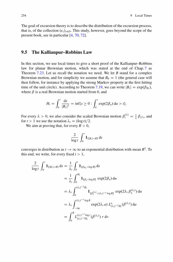
254 9 Local Times

The goal of excursion theory is to describe the distribution of the excursion process,that is, of the collection .es/s2D. This study, however, goes beyond the scope of thepresent book, see in particular [4, 70, 72].

9.5 The Kallianpur–Robbins Law

In this section, we use local times to give a short proof of the Kallianpur–Robbinslaw for planar Brownian motion, which was stated at the end of Chap. 7 asTheorem 7.23. Let us recall the notation we need. We let B stand for a complexBrownian motion, and for simplicity we assume that B0 D 1 (the general case willthen follow, for instance by applying the strong Markov property at the first hittingtime of the unit circle). According to Theorem 7.19, we can write jBtj D exp.ˇHt /,where ˇ is a real Brownian motion started from 0, and

Ht DZ t

0

ds

jBsj2 D inffs � 0 WZ s

0

exp.2ˇu/ du > tg:

For every � > 0, we also consider the scaled Brownian motion ˇ.�/t D 1�ˇ�2t, and

for t > 1 we use the notation �t D .log t/=2.We aim at proving that, for every R > 0,

2

log t

Z t

0

1fjBsj<Rg ds

converges in distribution as t ! 1 to an exponential distribution with mean R2. Tothis end, we write, for every fixed t > 1,

2

log t

Z t

0

1fjBsj<Rg ds D 1

�t

Z t

0

1fˇHs<log Rg ds

D 1

�t

Z Ht

0

1fˇu<log Rg exp.2ˇu/ du

D �t

Z .�t/�2Ht

0

1fˇ.�t/u <.�t/�1 log Rg exp.2�t ˇ

.�t/u / du

D �t

Z .�t/�1 log R

�1exp.2�t a/ La

.�t/�2Ht.ˇ.�t// da

DZ R

0

L.�t/�1 log r

.�t/�2Ht.ˇ.�t// r dr:

Exercises 255

In the second last equality, we applied the density of occupation time formula(Corollary 9.7) to the Brownian motion ˇ.�t/, and in the last one we used the changeof variables r D e�ta. As t ! 1, .�t/

�1 log r �! 0, for every r > 0, andLemma 7.21 also tells us that .�t/

�2Ht � T.�t/1 converges in probability to 0, with

the notation T.�/1 D inffs � 0 W ˇ.�/s D 1g. From the joint continuity of Brownianlocal times (Theorem 9.12), we then get that, for every " 2 .0;R/,

sup"�r�R

ˇ̌ˇL.�t/

�1 log r.�t/�2Ht

.ˇ.�t//� L0T.�t /1

.ˇ.�t//ˇ̌ˇ �!

t!1 0;

in probability. By combining this with the previous display, we obtain that

ˇ̌ˇ 2

log t

Z t

0

1fjBsj<Rg ds � R2

2L0

T.�t /1

.ˇ.�t//ˇ̌ˇ �!

t!1 0;

in probability. To complete the proof, we just note that the law of L0T.�/1

.ˇ.�// does

not depend on � > 0, and is exponential with mean 2, by Proposition 9.13.

Remark The preceding proof shows that the limiting exponential variable inTheorem 7.23 does not depend on the choice of R, in the sense that we can obtain ajoint convergence by taking several values of R, with the same exponential variablein the limit, up to multiplicative constants. This can also be deduced from theChacon–Ornstein ergodic theorem, which implies that the same limit in distributionholds more generally for the occupation time of an arbitrary compact subset K ofC, the constant R2 then being replaced by ��1 times the Lebesgue measure of K.Our method of proof also shows that the convergence in the Kallianpur–Robbinstheorem holds jointly with that of windings in Spitzer’s theorem (Theorem 7.20)and the limiting joint distribution is the law of .R2

2L0T1 .ˇ/; �T1 /, where ˇ and � are

independent real Brownian motions started from 0, and T1 D infft � 0 W ˇt D 1g.

Exercises

Exercise 9.16 Let f W R �! R be a monotone increasing function, and assume thatf is a difference of convex functions. Let X be a semimartingale and consider thesemimartingale Yt D f .Xt/. Prove that, for every a 2 R,

Lat .Y/ D f 0C.a/ La

t .X/; La�t .Y/ D f 0�.a/ La�

t .X/:

In particular, if X is a Brownian motion, the local times of f .X/ are continuous inthe space variable if and only if f is continuously differentiable.

256 9 Local Times

Exercise 9.17 Let M be a continuous local martingale such that hM;Mi1 D 1a.s., and let B be the Brownian motion associated with M via the Dambis–Dubins–Schwarz theorem (Theorem 5.13). Prove that, a.s. for every a � 0 and t � 0,

Lat .M/ D La

hM;Mit.B/:

Exercise 9.18 Let X be a continuous semimartingale, and assume that X can bewritten in the form

Xt D X0 CZ t

0

�.!; s/ dBs CZ t

0

b.!; s/ ds;

where B is a Brownian motion and � and b are progressive and locally bounded.Assume that �.!; s/ 6D 0 for Lebesgue a.e. s � 0, a.s. Show that the local timesLa

t .X/ are jointly continuous in the pair .a; t/.

Exercise 9.19 Let X be a continuous semimartingale. Show that the property

supp.dsLas .X// � fs � 0 W Xs D ag

holds simultaneously for all a 2 R, outside a single set of probability zero.

Exercise 9.20 Let B be a Brownian motion started from 0. Show that a.s. thereexists an a 2 R such that the inclusion supp.dsLa

s .B// � fs � 0 W Bs D ag is not anequality. (Hint: Consider the maximal value of B over Œ0; 1�.)

Exercise 9.21 Let B be a Brownian motion started from 0. Note thatZ 1

0

1fBs>0gds D 1

a.s. and set, for every t � 0,

At DZ t

0

1fBs>0gds ; �t D inffs � 0 W As > tg:

1. Verify that the process

�t DZ �t

0

1fBs>0gdBs

is a Brownian motion in an appropriate filtration.2. Show that the process �t D L0�t

.B/ has nondecreasing and continuous samplepaths, and that the support of the measure ds�s is contained in fs W B�s D 0g.

3. Show that the process .B�t /t�0 has the same distribution as .jBtj/t�0.

Exercises 257

Exercise 9.22 (Skew Brownian motion) Let ˛; ˇ > 0 and consider the functiong.x/ D ˛1fx�0g � ˇ1fx<0g. Let X be a continuous semimartingale such that

Xt DZ t

0

g.Xs/ dBs; (9.19)

where B is a Brownian motion.

1. Set '.x/ D 1˛

x 1fx�0g � 1ˇ

x 1fx<0g, and Yt D '.Xt/. Prove that Yt D '.Xt/ solvesthe equation

Yt D Bt C 1

2.1 � ˛

ˇ/ L0t .Y/

(use the result of Exercise 9.16).2. Compute L0t .Y/ � L0�t .Y/ in terms of L0t .Y/, in two different ways.3. Starting from a Brownian motion ˇ with ˇ0 D 0, set

At DZ t

0

ds

g.ˇs/2; �t D inffs � 0 W As > tg:

Verify that the process Xt D ˇ�t satisfies the equation (9.19) in an appropriatefiltration and with an appropriate Brownian motion B.

Exercise 9.23 Let g W R �! R be a real integrable function (RR

jg.x/jdx < 1).Let B be a Brownian motion started from 0, and set

At DZ t

0

g.Bs/ ds:

1. Justify the fact that the integral defining At makes sense, and verify that, for everyc > 0 and every u � 0, Ac2u has the same distribution as

c2Z u

0

g.c Bs/ ds:

2. Prove that

1pt

At.d/�!

t!1� Z

g.x/ dx�

jNj;

where N is N .0; 1/.

Exercise 9.24 Let � and b be two locally bounded measurable functions on RC�R,and consider the stochastic differential equation

E.�; b/ dXt D �.t;Xt/ dBt C b.t;Xt/ dt:

258 9 Local Times

Let X and X0 be two solutions of E.�; b/, on the same filtered probability space andwith the same Brownian motion B.

1. Suppose that L0t .X � X0/ D 0 for every t � 0. Show that both Xt _ X0t and Xt ^ X0

tare also solutions of E.�; b/. (Hint: Write Xt _ X0

t D Xt C .X0t � Xt/

C, and useTanaka’s formula.)

2. Suppose that �.t; x/ D 1 for every t; x. Show that the assumption in question 1.holds automatically. Suppose in addition that weak uniqueness holds for E.�; b/.Show that, if X0 D X0

0 D x 2 R, the two processes X and X0 are indistinguishable.

Exercise 9.25 (Another look at the Yamada–Watanabe criterion) Let � be a nonde-creasing function from Œ0;1/ into Œ0;1/ such that, for every " > 0,

Z "

0

du

�.u/D 1:

Consider then the one-dimensional stochastic differential equation

E.�; b/ dXt D �.Xt/dBt C b.Xt/dt

where one assumes that the functions � and b satisfy the conditions

.�.x/ � �.y//2 � �.jx � yj/ ; jb.x/� b.y/j � K jx � yj ;

for every x; y 2 R, with a constant K < 1. Our goal is use local times to givea short proof of pathwise uniqueness for E.�; b/ (this is slightly stronger than theresult of Exercise 8.14).

1. Let Y be a continuous semimartingale such that, for every t > 0,

Z t

0

dhY;Yis

�.jYsj/ < 1; a.s.

Prove that L0t .Y/ D 0 for every t � 0, a.s.2. Let X and X0 be two solutions of E.�; b/ on the same filtered probability space

and with the same Brownian motion B. By applying question 1. to Y D X � X0,prove that L0t .X � X0/ D 0 for every t � 0, a.s., and therefore,

jXt � X0t j D jX0 � X0

0j CZ t

0

.�.Xs/ � �.X0s// sgn.Xs � X0

s/ dBs

CZ t

0

.b.Xs/ � b.X0s// sgn.Xs � X0

s/ ds:

3. Using Gromwall’s lemma, prove that if X0 D X00 then Xt D X0

t for every t � 0,a.s.


Notes and Comments

The local time of Brownian motion was first discussed by Lévy [54] under thename “mesure du voisinage”. In 1958, Trotter [80] established the joint continuityof Brownian local times viewed as densities of the occupation measure. Tanaka [79]obtained the formulas of Proposition 9.2 in the Brownian case. The local time ofsemimartingales was discussed by Meyer [61], who derived Theorem 9.6 in thisgeneral setting (after the earlier work of Tanaka [79] in the Brownian setting).Yor [84] then developed the powerful approach that leads to Theorem 9.4. Theupcrossing approximation of local time (Proposition 9.11) is due to Itô and McKean[42, Chapter 2] for Brownian motion, and was extended to semimartingales by ElKaroui [22]. Other approximation results for the Brownian local time were obtainedby Lévy [54] (see [42] and [70]). Theorem 9.14 is essentially due to Lévy [54], butour proof is based on an argument from Skorokhod [74] (see [23] for a related studyof the so-called “reflection problem” in the semimartingale setting). For furtherproperties of local times, the reader may consult Chapter V of [70] or Chapter 6of [49], as well as the classical book [42] of Itô and McKean. Local times arealso a key ingredient of excursion theory, which is treated in the general setting ofMarkov processes in Blumenthal’s book [4]. Exercise 9.22 deals with the singularstochastic equation first studied by Harrison and Shepp [31], whose solution is theso-called skew Brownian motion. Exercise 9.23 gives the one-dimensional versionof the Kallianpur–Robbins law, which can also be found in [48]. Exercise 9.25 isfrom [51].

Erratum to: Brownian Motion, Martingales,and Stochastic Calculus


Erratum to:J.-F. Le Gall, Brownian Motion, Martingales, and Stochastic Calculus,Graduate Texts in Mathematics 274, DOI 10.1007/978-3-319-31089-3© Springer International Publishing Switzerland 2016

The following information about the original edition was missing in the front-matter:

Translated from the French language edition:‘Mouvement brownien, martingales et calcul stochastique’ by Jean-François Le GallCopyright © Springer-Verlag Berlin Heidelberg 2013Springer International Publishing is part of Springer Science+Business MediaAll Rights Reserved.

The online version of the updated book can be found underDOI 10.1007/978-3-319-31089-3

Jean-François Le GallDépartement de MathématiquesUniversité Paris-SudOrsay Cedex, France


E1

Appendix A1The Monotone Class Lemma

The monotone class lemma is a tool of measure theory which is very useful inseveral arguments of probability theory. We give here the version of this lemma thatis used in several places in this volume.

Let E be an arbitrary set, and let P.E/ denote the set of all subsets of E. IfC � P.E/, �.C / stands for the smallest �-field on E containing C (it is also theintersection of all �-fields containing C ).

Definition A subset M of P.E/ is called a monotone class if the followingproperties hold:

(i) E 2 M .(ii) If A;B 2 M and A � B, then BnA 2 M .

(iii) If .An/n�0 is an increasing sequence of subsets of E such that An 2 M for

every n � 0, then[n�0

An 2 M .

A �-field is a monotone class. As in the case of �-fields, one immediatelychecks that the intersection of an arbitrary collection of monotone classes is again amonotone class. If C is an arbitrary subset of P.E/, the monotone class generatedby C , which is denoted by M .C /, is defined by setting

M .C / D\

M monotone class; C�M

M :

Monotone class lemma If C � P.E/ is stable under finite intersections, thenM .C / D �.C /.

Proof Since any �-field is a monotone class, it is clear that M .C / � �.C /. Toprove the reverse inclusion, it is enough to verify that M .C / is a �-field. However,a monotone class is a �-field if and only if it is stable under finite intersections(indeed, considering the complementary sets shows that it is then stable under finite

© Springer International Publishing Switzerland 2016J.-F. Le Gall, Brownian Motion, Martingales, and Stochastic Calculus,Graduate Texts in Mathematics 274, DOI 10.1007/978-3-319-31089-3

261

262 A1 The Monotone Class Lemma

unions, and via an increasing passage to the limit one gets that it is also stable undercountable unions). Let us show that M .C / is stable under finite intersections.

For every A 2 P.E/, set

MA D fB 2 M .C / W A \ B 2 M .C /g:

Fix A 2 C . Since C is stable under finite intersections, we have C � MA. Let usverify that MA is a monotone class:

• E 2 MA is trivial.• If B;B0 2 MA and B � B0, we have A \ .B0nB/ D .A \ B0/n.A \ B/ 2 M .C /

and thus B0nB 2 MA.• If Bn 2 MA for every n � 0 and the sequence .Bn/n�0 is increasing, we have

A \ .[Bn/ D [.A \ Bn/ 2 M .C / and therefore [Bn 2 MA.

Since MA is a monotone class that contains C , MA also contains M .C /. We havethus obtained that

8A 2 C ; 8B 2 M .C /; A \ B 2 M .C /:

This is not yet the desired result, but we can use the same idea another time.Precisely, we now fix A 2 M .C /. According to the first part of the proof, C � MA.By exactly the same arguments as in the first part of the proof, we get that MA isa monotone class. It follows that M .C / � MA, which shows that M .C / is stableunder finite intersections, and completes the proof. ut

Here are a few consequences of the monotone class lemma that are used above.

1. Let A be a �-field on E, and let and be two probability measures on.E;A /. Assume that there exists a class C � A , which is stable under finiteintersections, such that �.C / D A and .A/ D .A/ for every A 2 C . Then D . (Use the fact that G WD fA 2 A W .A/ D .A/g is a monotone class.)

2. Let .Xi/i2I be an arbitrary collection of random variables, and let G be a �-fieldon the same probability space. In order to show that the �-fields �.Xi; i 2 I/ andG are independent, it is enough to verify that .Xi1 ; : : : ;Xip/ is independent of G ,for any choice of the finite set fi1; : : : ; ipg � I. (Observe that the class of allevents that depend on a finite number of the variables Xi; i 2 I, is stable underfinite intersections and generates �.Xi; i 2 I/.)

3. Let .Xi/i2I be an arbitrary collection of random variables, and let Z be a boundedreal variable. Let i0 2 I. In order to verify that EŒZ j Xi; i 2 I� D EŒZ j Xi0 �, itis enough to show that EŒZ j Xi0 ;Xi1 ; : : : ;Xip � D EŒZ j Xi0 � for any choice of thefinite collection fi1; : : : ; ipg � I. (Observe that the class of all events A such thatEŒ1AZ� D EŒ1A EŒZ j Yi0 �� is a monotone class.)

This last consequence of the monotone class lemma is useful in the theory ofMarkov processes.

Appendix A2Discrete Martingales

In this appendix, we recall without proof the results about discrete time martingalesand supermartingales that are used in Chap. 3. The proof of the subsequentstatements can be found in Neveu’s book [65], and in many other books dealingwith discrete time martingales (see in particular Williams [82] and Chapter XII inGrimmett and Stirzaker [30]).

We use the notation N D f0; 1; 2; : : :g. Let us start by recalling the basingdefinitions. We consider a probability space .˝;F ;P/, and we fix a discretefiltration, that is, an increasing sequence .Gn/n2N of sub-�-fields of F . We also let

G1 D1_

nD0Gn

be the smallest �-field that contains all the �-fields Gn.

Definition A sequence .Yn/n2N of integrable random variables, such that Yn isGn-measurable for every n 2 N, is called

• a martingale if, whenever 0 � m < n, EŒYn j Gm� D Ym;• a supermartingale if, whenever 0 � m < n, EŒYn j Gm� � Ym;• a submartingale if, whenever 0 � m < n, EŒYn j Gm� � Ym.

All these notions obviously depend on the choice of the filtration .Gn/n2N, whichis fixed in what follows.

Maximal inequality If .Yn/n2N is a supermartingale, then, for every � > 0 andevery k 2 N,

�P�

supn�k

jYnj > ��

� EŒjY0j�C 2EŒjYkj�:


263

264 A2 Discrete Martingales

Doob’s inequality in Lp If .Yn/n2N is a martingale, then, for every k 2 N and everyp > 1,

Eh

sup0�n�k

jYnjpi

�� p

p � 1�p

EŒjYkjp�:

Remark This inequality is interesting only if EŒjYkjp� < 1, since otherwise bothsides are infinite.

If y D .yn/n2N is a sequence of real numbers, and a < b, the upcrossing numberof this sequence along Œa; b� before time n, denoted by My

ab.n/, is the largest integerk such that there exists a strictly increasing finite sequence

m1 < n1 < m2 < n2 < � � � < mk < nk

of nonnegative integers smaller than or equal to n with the properties ymi � a andyni � b, for every i 2 f1; : : : ; kg. In what follows we consider a sequence Y D.Yn/n2N of real random variables, and the associated upcrossing number MY

ab.n/ isthen an integer-valued random variable.

Doob’s upcrossing inequality If .Yn/n2N is a supermartingale, then, for every n 2N and every a < b,

EŒMYab.n/� � 1

b � aEŒ.Yn � a/��:

This inequality is a crucial tool for proving the convergence theorems fordiscrete-time martingales and supermartingales. Let us recall two importantinstances of these theorems.

Convergence theorem for discrete-time supermartingales If .Yn/n2N is a super-martingale, and if the sequence .Yn/n2N is bounded in L1, then there exists a randomvariable Y1 2 L1 such that

Yna:s:�!

n!1 Y1:

Convergence theorem for uniformly integrable discrete-time martingales Let.Yn/n2N be a martingale. The following are equivalent:

(i) The martingale .Yn/n2N is closed, in the sense that there exists a randomvariable Z 2 L1.˝;F ;P/ such that Yn D EŒZ j Gn� for every n 2 N.

(ii) The sequence .Yn/n2N converges a.s. and in L1.(iii) The sequence .Yn/n2N is uniformly integrable.

If these properties hold, the a.s. limit of the sequence .Yn/n2N is Y1 D EŒZ j G1�.

A2 Discrete Martingales 265

We now recall two versions of the optional stopping theorem in discrete time.A (discrete) stopping time is a random variable T with values in N [ f1g, suchthat fT D ng 2 Gn for every n 2 N. The �-field of the past before T is thenGT D fA 2 G1 W A \ fT D ng 2 Gn; for every n 2 Ng.

Optional stopping theorem for uniformly integrable discrete-time martingalesLet .Yn/n2N be a uniformly integrable martingale, and let Y1 be the a.s. limit of Yn

when n ! 1. Then, for every choice of the stopping times S and T such that S � T,we have YT 2 L1 and

YS D EŒYT j GS�

with the convention that YT D Y1 on the event fT D 1g, and similarly for YS.

Optional stopping theorem for discrete-time supermartingales (bounded case)If .Yn/n2N is a supermartingale, then, for every choice of the bounded stopping timesS and T such that S � T, we have

YS � EŒYT j GS�:

We conclude with a variant of the convergence theorem for supermartingales inthe backward case. We consider a backward filtration, that is, an increasing sequenceof filtrations .Hn/n2�N indexed by negative integers (in such a way that the �-fieldHn is “smaller and smaller” when n ! �1). A sequence .Yn/n2�N of integrablerandom variables indexed by negative integers is called a backward supermartingaleif, for every n 2 �N, Yn is Hn-measurable and, for every m � n � 0,EŒYn j Hm� � Ym.

Convergence theorem forbackwarddiscrete-time supermartingales If .Yn/n2�N

is a backward supermartingale, and if the sequence .Yn/n2�N is bounded in L1, thenthe sequence .Yn/n2�N converges a.s. and in L1 when n ! �1.

It is crucial for the applications developed in Chap. 3 that the convergence alsoholds in L1 in the backward case (compare with the analogous result in the “forward”case).

References

1. Adler, R.J.: An Introduction to Continuity, Extrema and Related Topics for General GaussianProcesses. Institute of Mathematical Statistics, Hayward (1990)

2. Bachelier, L.: Théorie de la spéculation. Ann. Sci. Ecole Norm. Sup. 17, 21–86 (1900)3. Bertoin, J.: Lévy Processes. Cambridge University Press, Cambridge (1996)4. Blumenthal, R.M.: Excursions of Markov Processes. Birkhäuser, Boston (1992)5. Blumenthal, R.M., Getoor, R.K.: Markov Processes and Potential Theory. Academic,

New York (1968)6. Burkholder, D.L.: Distribution function inequalities for martingales. Ann. Probab. 1, 19–42

(1973)7. Burkholder, D.L., Davis, B.J., Gundy, R.F.: Integral inequalities for convex functions of

operators on martingales. In: Proceedings of Sixth Berkeley Symposium on MathematicalStatistics and Probability, vol. 2, pp. 223–240. University of Calfornia Press, Berkeley (1972)

8. Cameron, R.H., Martin, W.T.: Transformation of Wiener integrals under translations. Ann.Math. 45, 386–396 (1944)

9. Chung, K.L.: Lectures from Markov Processes to Brownian Motion. Springer, Berlin (1982)10. Chung, K.L., Williams, R.J.: Introduction to Stochastic Integration. Birkhäuser, Boston (1983)11. Dambis, K.E.: On the decomposition of continuous martingales. Theor. Probab. Appl. 10, 401–

410 (1965)12. Davis, B.J.: Brownian motion and analytic functions. Ann. Probab. 7, 913–932 (1979)13. Dellacherie, C., Meyer, P.-A.: Probabilités et potentiel, Chapitres I à IV. Hermann, Paris (1975)14. Dellacherie, C., Meyer, P.-A.: Probabilités et potentiel, Chapitres V à VIII. Théorie des

martingales. Hermann, Paris (1980)15. Doob, J.L.: Stochastic Processes. Wiley, New York (1953)16. Doob, J.L.: Classical Potential Theory and its Probabilistic Counterpart. Springer, Berlin

(1984)17. Dubins, L., Schwarz, G.: On continuous martingales. Proc. Nat. Acad. Sci. USA 53, 913–916

(1965)18. Durrett, R.: Brownian Motion and Martingales in Analysis. Wadsworth, Belmont (1984)19. Dynkin, E.B.: Inhomogeneous strong Markov processes. Dokl. Akad. Nauk. SSSR 113, 261–

263 (1957)20. Dynkin, E.B.: Theory of Markov Processes. Pergamon, Oxford (1960)21. Dynkin, E.B.: Markov Processes (2 Volumes). Springer, Berlin (1965)22. El Karoui, N.: Sur les montées des semimartingales. Astérisque 52–53, 63–88 (1978)


267

268 References

23. El Karoui, N., Chaleyat-Maurel, M.: Un problème de réflexion et ses applications au rempslocal et aux équations différentielles stochastiques sur R, cas continu. Astérisque 52–53, 117–144 (1978)

24. Ethier, S.N., Kurtz, T.G.: Markov Processes: Characterization and Convergence. Wiley,New York (1986)

25. Fisk, D.L.: Quasimartingales. Trans. Am. Math. Soc. 120, 369–389 (1965)26. Friedman, A.: Stochastic Differential Equations and Applications, vol. 1. Academic Press,

New York (1975)27. Friedman, A.: Stochastic Differential Equations and Applications, vol. 2. Academic Press,

New York (1976)28. Getoor, R.K., Sharpe, M.J.: Conformal martingales. Invent. Math. 16, 271–308 (1972)29. Girsanov, I.V.: On transforming a certain class of stochastic processes by absolutely continuous

substitution of measures. Theory Probab. Appl. 5, 285–301 (1960)30. Grimmett, G.R., Stirzaker, D.R.: Probability and Random Processes. Oxford University Press,

Oxford (1992)31. Harrison, J.M., Shepp, L.A.: On skew Brownian motion. Ann. Probab. 9, 309–313 (1981)32. Hunt, G.A.: Some theorems concerning Brownian motion. Trans. Am. Math. Soc. 81, 294–319

(1956)33. Hunt, G.A.: Markov processes and potentials. Ill. J. Math. 1, 44–93 (1957)34. Hunt, G.A.: Markov processes and potentials. Ill. J. Math.2, 151–213 (1957)35. Ikeda, N., Watanabe, S.: Stochastic Differential Equations and Diffusion Processes. North-

Holland, Amsterdam/New York (1981)36. Itô, K.: Stochastic integral. Proc. Imp. Acad. Tokyo 20, 518–524 (1944)37. Itô, K.: On a stochastic integral equation. Proc. Imp. Acad. Tokyo 22, 32–35 (1946)38. Itô, K.: On stochastic differential equations. Mem. Am. Math. Soc. 4, 1–51 (1951)39. Itô, K.: Multiple Wiener integral. J. Math. Soc. Jpn. 3, 157–169 (1951)40. Itô, K.: On a formula concerning stochastic differentials. Nagoya Math. J. 3, 55–65 (1951)41. Itô, K.: Selected Papers. Edited and with an Introduction by S.R.S. Varadhan and D.W. Stroock.

Springer, New York (1987)42. Itô, K., McKean, H.P.: Diffusion Processes and their Sample Paths. Springer, Berlin (1965)43. Itô, K., Watanabe, S.: Transformation of Markov processes by multiplicative functionals. Ann.

Inst. Fourier 15, 15–30 (1965)44. Jacod, J., Shiryaev, A.: Limit Theorems for Stochastic Processes. Springer, Berlin (2003)45. Kakutani, S.: On Brownian motion in n-space. Proc. Imp. Acad. Tokyo 20, 648–652 (1944)46. Kakutani, S.: Two-dimensional Brownian motion and harmoinc functions. Proc. Imp. Acad.

Tokyo 20, 706–714 (1944)47. Kallenberg, O.: Foundations of Modern Probability. Springer, Berlin/Heidelberg/New York

(2002)48. Kallianpur, G., Robbins, H.: Ergodic property of Brownian motion process. Proc. Nat. Acad.

Sci. USA 39, 525–533 (1953)49. Karatzas, I., Shreve, S.: Brownian Motion and Stochastic Calculus. Springer, Berlin (1987)50. Kunita, H., Watanabe, S.: On square-integrable martingales. Nagoya J. Math. 36, 1–26 (1967)51. Le Gall, J.-F.: Applications du temps local aux équations différentielles stochastiques unidi-

mensionnelles. In: Lectures Notes in Mathematics, vol. 986, pp. 15–31. Springer, Berlin (1983)52. Le Gall, J.-F.: Some Properties of Planar Brownian Motion. Lecture Notes in Mathematics,

vol. 1527, pp. 111–235. Springer, Berlin (1992)53. Lévy, P.: Le mouvement brownien plan. Am. J. Math. 62, 487–550 (1940)54. Lévy, P.: Processus stochastiques et mouvement brownien. Gauthier-Villars, Paris (1948)55. Lifshits, M.A.: Gaussian Random Functions. Kluwer Academic, Dordrecht (1995)56. Marcus, M.B., Rosen, J.: Markov Processes, Gaussian Processes, and Local Times. Cambridge

University Press, Cambridge (2006)57. McKean, H.P.: Stochastic Integrals. Academic, New York (1969)58. Meyer, P.-A.: A decomposition theorem for supermartingales. Ill. J. Math. 6, 193–205 (1962)

References 269

59. Meyer, P.-A.: Processus de Markov. Lecture Notes in Mathamatics, vol. 26. Springer, Berlin(1967)

60. Meyer, P.-A.: Intégrales stochastiques. In: Lecture Notes Mathamatics, vol. 39, pp. 72–162.Springer, Berlin (1967)

61. Meyer, P.-A.: Un cours sur les intégrales stochastiques. In: Lecture Notes in Mathamatics,vol. 511, pp. 245–400. Springer, Berlin (1976)

62. Mörters, P., Peres, Y.: Brownian Motion. Cambridge University Press, Cambridge (2010)63. Protter, P.: Stochastic Integration and Differential Equations. Springer, Berlin (2005)64. Neveu, J.: Mathematical Foundations of the Calculus of Probability. Holden–Day,

San Francisco (1965)65. Neveu, J.: Discrete-Parameter Martingales. North-Holland, Amsterdam (1975)66. Øksendal, B.: Stochastic Differential Equations. An Introduction with Applications. Springer,

Berlin (2003)67. Pitman, J.W., Yor, M.: A decomposition of Bessel bridges. Z. Wahrscheinlichkeitstheorie verw.

Gebiete 59, 425–457 (1982)68. Pitman, J.W., Yor, M.: Asymptotic laws of planar Brownian motion. Ann. Probab. 14, 733–779

(1986)69. Port, S.C., Stone, C.J.: Brownian Motion and Classical Potential Theory. Academic Press,

New York (1978)70. Revuz, D., Yor, M.: Continuous Martingales and Brownian Motion. Springer, Berlin (1991)71. Rogers, L.C.G., Williams, D.: Diffusions, Markov Processes and Martingales, vol. 1: Founda-

tions. Wiley, New York (1994)72. Rogers, L.C.G., Williams, D.: Diffusions, Markov Processes and Martingales, vol. 2: Itô

calculus. Wiley, New York (1987)73. Sharpe, M.J.: General Theory of Markov Processes. Academic, New York (1989)74. Skorokhod, A.V.: Stochastic equations for diffusion processes in a bounded domain. Theory

Probab. Appl. 6, 264–274 (1961)75. Spitzer, F.: Some theorems concerning two-dimensional Brownian motion. Trans. Am. Math.

Soc. 87, 187–197 (1958)76. Stroock, D.W.: An Introduction to Markov Processes. Springer, Berlin (2005)77. Stroock, D.W., Varadhan, S.R.S.: Multidimensional Diffusion Processes. Springer, Berlin

(1979)78. Talagrand, M.: The Generic Chaining. Springer, Berlin (2005)79. Tanaka, H.: Note on continuous additive functionals of the 1-dimensional Brownian path.

Z. Wahrscheinlichkeitstheorie verw. Gebiete 1, 251–257 (1963)80. Trotter, H.F.: A property of Brownian motion paths. Ill. J. Math. 2, 425–433 (1958)81. Wiener, N.: Differential space. J. Math. Phys. 2, 132–174 (1923)82. Williams, D.: Probability with Martingales. Cambridge University Press, Cambridge (1991)83. Yamada, T., Watanabe, S.: On the uniqueness of solutions of stochastic differential equations.

J. Math. Kyoto Univ. 11, 155–167 (1971)84. Yor, M.: Sur la continuité des temps locaux associés à certaines semimartingales. Astérisque

52–53, 23–36 (1978)

Index

� -field of the past before a stopping time, 44Brownian case, 33

approximation of a stochastic integral, 112arcsine law, 39associativity of stochastic integrals, 105, 110

Bessel process, 145, 227Blumenthal’s zero-one law, 30bracket

of two continuous local martingales, 87of two independent Brownian motions, 88of two semimartingales, 90

Brownian bridge, 38Brownian motion, 27.Ft/-Brownian motion, 116.Ft/-Brownian motion, 50canonical construction, 29multidimensional, 37, 148, 196sample paths properties, 29

Burkholder–Davis–Gundy inequalities, 124

càdlàg function, 54càdlàg sample paths

for a Feller process, 164for a supermartingale, 55for semimartingale local times, 239

Cameron–Martin formula, 139canonical decomposition of a semimartingale,

90canonical process, 29complex Brownian motion, 198

conditioning of Gaussian variables, 9conformal invariance of Brownian motion,

198constancy intervals of a martingale, 121continuity of sample paths, 24

for Brownian local times, 249for Brownian martingales, 130for Brownian motion, 27

continuity of the Brownian filtration, 129continuous semimartingale, 90continuous-state branching process, 177convergence theorem for stochastic integrals,

111covariance function, 10cylinder set, 28

Dambis–Dubins–Schwarz theorem, 121density of occupation time formula, 245diffusion process, 224Dirichlet problem, 189domain of the generator, 159Doob’s inequality in Lp , 53

in discrete time, 264Doob’s upcrossing inequality, 264Dynkin’s formula, 182

excursions of Brownian motion, 253exit distribution from a ball, 195exit distribution from an annulus, 196exponential martingale, 118

of Brownian motion, 51exterior cone condition, 191


271

272 Index

Feller process, 158solution of an SDE, 222

Feller semigroup, 158Feller’s branching diffusion, 179, 227Feynman–Kac formula, 181, 187, 206filtered probability space, 41filtration, 41

complete, 42right-continuous, 42

finite variation process, 73finite-dimensional marginal distributions

for a Gaussian process, 10for a Markov process, 153for Brownian motion, 21

formula of integration by parts, 116function with finite variation, 69

total variation, 70

Gaussian process, 7Gaussian space, 7Gaussian variable, 1Gaussian vector, 4Gaussian white noise, 11generator of a Feller semigroup, 159

case of a jump process, 172case of Brownian motion, 161case of the solution of an SDE, 222

geometric Brownian motion, 226Girsanov’s theorem, 134Gronwall’s lemma, 213

harmonic function, 187radial, 193

heat equation, 185hitting time of a set, 48

independence of Gaussian variables, 8indistinguishable, 23integral with respect to a finite variation

process, 74intensity of a Gaussian white noise, 11invariance properties of Brownian motion, 22inverse local time, 252Itô’s formula, 113

case of Brownian motion, 116extension to a function defined on an open

set, 117generalized, 244

jump Markov process, 170transition rate, 173

Kallianpur–Robbins law, 205Kalman filtering, 15Kazamaki’s criterion, 136Kolmogorov’s extension theorem, 10, 154Kolmogorov’s lemma, 24Kunita–Watanabe inequality, 88

Lévy area, 144Lévy process, 175Lévy’s construction of Brownian motion, 16Lévy’s theorem, 119Lévy’s theorem on Brownian local time, 252law of Brownian hitting times, 37

case with drift, 140Laplace transform, 63

law of the exit point from an interval, 62law of the exit time from an interval, 63, 66law of the iterated logarithm, 39local martingale, 75local maxima of Brownian paths, 39local time

continuity in the space variable, 239definition, 237of Brownian motion, 249support property, 238upcrossing approximation, 248

Markov process, 152canonical construction, 155solution of an SDE, 221

martingale, 49closed, 59convergence theorem, 59discrete-time, 263regularity of sample paths, 55stopped at a stopping time, 61uniformly integrable, 59

maximal inequality, 53in discrete time, 263

mean value property, 188modification, 23moments of stochastic integrals, 105, 108monotone class lemma, 261

non-differentiability of Brownian paths, 39Novikov’s criterion, 136

optional stopping theorem, 59discrete case, 265for nonnegative supermartingales, 64

Index 273

Ornstein–Uhlenbeck process, 225orthogonal local martingales, 88

pathwise uniqueness for an SDE, 211planar Brownian motion, 198

asymptotic laws, 201Poisson kernel, 193polar sets, 205polarity of points, 197pre-Brownian motion, 19process

adapted, 43elementary, 100measurable, 42progressive, 43

process with independent increments, 50associated martingales, 50

progressive � -field, 43, 99

quadratic variationof a continuous local martingale, 79of a semimartingale, 90of a stopped local martingale, 85of Brownian motion, 32, 79

quasi left-continuity of a Feller process, 181

random process, 7recurrence of planar Brownian motion, 197reflected Brownian motion, 179reflection principle, 35representation of Brownian martingales, 127resolvent of a transition semigroup, 156

sample paths of a random process, 23simple Markov property, 168

case of Brownian motion, 22skew-product decomposition, 199Spitzer’s theorem on Brownian windings, 201stationary Gaussian process, 11stochastic calculus with the supremum, 142stochastic differential equation, 210

Lipschitz case, 212

stochastic integralcase of a continuous local martingale, 106case of a finite variation process, 74case of a martingale bounded in L2, 101case of a semimartingale, 109

stopped process, 75stopping time, 44

case of Brownian motion, 33reducing a continuous local martingale, 76

strong Markov propertyof a Feller process, 169of Brownian motion, 34of the solution of an SDE, 224

strong solution of an SDE, 211submartingale, 49

discrete-time, 263supermartingale, 49

discrete-time, 263

Tanaka’s formula, 237time change, 121, 198

for constructing solutions of an SDE, 228time inversion, 38time reversal property of Brownian motion, 39transience of Brownian motion, 197transition kernel, 152transition semigroup, 152Trotter’s theorem, 249

upcrossing number, 54

weak existence for an SDE, 211weak uniqueness for an SDE, 211Wiener integral, 22, 108Wiener measure, 27

quasi-invariance property, 140

Yamada–Watanabe theorem, 212Yamada–Watanabe uniqueness criterion, 231

zero set of Brownian motion, 39, 253

Documents

link.springer.com...Graduate Texts in Mathematics Series Editors: Sheldon Axler San Francisco State University, San Francisco, CA, USA Kenneth Ribet University of …