Embed Size (px)
Citation preview
Link Analysis Ranking: Algorithms, Theory,and Experiments
ALLAN BORODINUniversity of TorontoGARETH O. ROBERTSLancaster UniversityJEFFREY S. ROSENTHALUniversity of TorontoandPANAYIOTIS TSAPARASUniversity of Helsinki
The explosive growth and the widespread accessibility of the Web has led to a surge of research ac-tivity in the area of information retrieval on the World Wide Web. The seminal papers of Kleinberg[1998, 1999] and Brin and Page [1998] introduced Link Analysis Ranking, where hyperlink struc-tures are used to determine the relative authority of a Web page and produce improved algorithmsfor the ranking of Web search results. In this article we work within the hubs and authorities frame-work defined by Kleinberg and we propose new families of algorithms. Two of the algorithms wepropose use a Bayesian approach, as opposed to the usual algebraic and graph theoretic approaches.We also introduce a theoretical framework for the study of Link Analysis Ranking algorithms. Theframework allows for the definition of specific properties of Link Analysis Ranking algorithms, aswell as for comparing different algorithms. We study the properties of the algorithms that we de-fine, and we provide an axiomatic characterization of the INDEGREE heuristic which ranks each nodeaccording to the number of incoming links. We conclude the article with an extensive experimentalevaluation. We study the quality of the algorithms, and we examine how different structures in thegraphs affect their performance.
Categories and Subject Descriptors: H.3.3 [Information Storage and Retrieval]: InformationSearch and Retrieval—Search process
General Terms: Algorithms, Theory
Additional Key Words and Phrases: Bayesian, HITS, link analysis, ranking, Web search
Authors’ addresses: A. Borodin, J. S. Rosenthal, University of Toronto, Toronto, Canada; email: [email protected]; G. O. Roberts, Lancaster University; P. Tsaparas, University of Helsinki, Helsinki,Finland; email: [email protected] to make digital or hard copies of part or all of this work for personal or classroom use isgranted without fee provided that copies are not made or distributed for profit or direct commercialadvantage and that copies show this notice on the first page or initial screen of a display alongwith the full citation. Copyrights for components of this work owned by others than ACM must behonored. Abstracting with credit is permitted. To copy otherwise, to republish, to post on servers,to redistribute to lists, or to use any component of this work in other works requires prior specificpermission and/or a fee. Permissions may be requested from Publications Dept., ACM, Inc., 1515Broadway, New York, NY 10036 USA, fax: +1 (212) 869-0481, or [email protected]© 2005 ACM 1533-5399/05/0200-0231 $5.00
ACM Transactions on Internet Technology, Vol. 5, No. 1, February 2005, Pages 231–297.
232 • A. Borodin et al.
1. INTRODUCTION
Ranking is an integral component of any information retrieval system. In thecase of Web search, because of the size of the Web and the special nature of theWeb users, the role of ranking becomes critical. It is common for Web searchqueries to have thousands or millions of results. On the other hand, Web usersdo not have the time and patience to go through them to find the ones theyare interested in. It has actually been documented [Broder 2002; Silversteinet al. 1998; Jansen et al. 1998] that most Web users do not look beyond the firstpage of results. Therefore, it is important for the ranking function to outputthe desired results within the top few pages, otherwise the search engine isrendered useless.
Furthermore, the needs of the users when querying the Web are differentfrom traditional information retrieval. For example, a user that poses the query“microsoft” to a Web search engine is most likely looking for the home page of Mi-crosoft Corporation, rather than the page of some random user that complainsabout the Microsoft products. In a traditional information retrieval sense, thepage of the random user may be highly relevant to the query. However, Webusers are most interested in pages that are not only relevant, but also authori-tative, that is, trusted sources of correct information that have a strong presencein the Web. In Web search, the focus shifts from relevance to authoritativeness.The task of the ranking function is to identify and rank highly the authoritativedocuments within a collection of Web pages.
To this end, the Web offers a rich context of information which is expressedthrough the hyperlinks. The hyperlinks define the “context” in which a Webpage appears. Intuitively, a link from page p to page q denotes an endorsementfor the quality of page q. We can think of the Web as a network of recommenda-tions which contains information about the authoritativeness of the pages. Thetask of the ranking function is to extract this latent information and producea ranking that reflects the relative authority of Web pages. Building upon thisidea, the seminal papers of Kleinberg [1998], and Brin and Page [1998] intro-duced the area of Link Analysis Ranking, where hyperlink structures are usedto rank Web pages.
In this article, we work within the hubs and authorities framework definedby Kleinberg [1998]. Our contributions are three-fold.
(1) We identify some potential weaknesses of the HITS algorithm, proposedby Kleinberg [1998], and we propose new algorithms that use alternativemethods for computing hub and authority weights. Two of our new algo-rithms are based on a Bayesian statistical approach as opposed to the morecommon algebraic/graph theoretic approach.
(2) We define a theoretical framework for the study of Link Analysis Rankingalgorithms. Within this framework, we define properties that characterizethe algorithms, such as monotonicity, stability, locality, label independence.We also define various notions of similarity between different Link Anal-ysis Ranking algorithms. The properties we define allow us to provide anaxiomatic characterization of the INDEGREE algorithm which ranks nodesaccording to the number of incoming links.
ACM Transactions on Internet Technology, Vol. 5, No. 1, February 2005.

Link Analysis Ranking: Algorithms, Theory and Experiments • 233
(3) We perform an extensive experimental evaluation of the algorithms on mul-tiple queries. We observe that no method is completely safe from “topicdrift”, but some methods seem to be more resistant than others. In orderto better understand the behavior of the algorithms, we study the graphstructures that they tend to favor. The study offers valuable insight intothe reasons that cause the topic drift and poses interesting questions forfuture research.
The rest of the article is structured as follows. In Section 2, we review some ofthe related literature and we introduce the notation we use in the article. InSection 3, we define the new Link Analysis Ranking algorithms. In Section 4,we define the theoretical framework for the study of Link Analysis Rankingalgorithms, and we provide some preliminary results. Section 5 presents theexperimental study of the Link Analysis Ranking algorithms, and Section 6concludes the article.
2. BACKGROUND AND PREVIOUS WORK
In this section, we present the necessary background for the rest of the article.We also review the literature in the area of link analysis ranking, upon whichthis work builds.
2.1 Preliminaries
A link analysis ranking algorithm starts with a set of Web pages. Dependingon how this set of pages is obtained, we distinguish between query independentalgorithms, and query dependent algorithms. In the former case, the algorithmranks the whole Web. The PAGERANK algorithm by Brin and Page [1998] wasproposed as a query independent algorithm that produces a PageRank valuefor all Web pages. In the latter case, the algorithm ranks a subset of Web pagesthat is associated with the query at hand. Kleinberg [1998] describes how toobtain such a query dependent subset. Using a text-based Web search engine,a Root Set is retrieved consisting of a short list of Web pages relevant to a givenquery. Then, the Root Set is augmented by pages which point to pages in theRoot Set, and also pages which are pointed to by pages in the Root Set, to obtaina larger Base Set of Web pages. This is the query dependent subset of Web pageson which the algorithm operates.
Given the set of Web pages, the next step is to construct the underlyinghyperlink graph. A node is created for every Web page, and a directed edge isplaced between two nodes if there is a hyperlink between the correspondingWeb pages. The graph is simple. Even if there are multiple links between twopages, only a single edge is placed. No self-loops are allowed. The edges could beweighted using, for example, content analysis of the Web pages, similar to thespirit of the work of Bharat and Henzinger [1998]. In our work, we will assumethat no weights are associated with the edges of the graph. Usually links withinthe same Web site are removed since they do not convey an endorsement; theyserve the purpose of navigation. Isolated nodes are removed from the graph.
Let P denote the resulting set of nodes, and let n be the size of the set P .Let G = (P, E) denote the underlying graph. The input to the link analysis
ACM Transactions on Internet Technology, Vol. 5, No. 1, February 2005.

234 • A. Borodin et al.
algorithm is the adjacency matrix W of the graph G, where W [i, j ] = 1 if thereis a link from node i to node j , and zero otherwise. The output of the algorithmis an n-dimensional vector a, where ai, the i-th coordinate of the vector a, isthe authority weight of node i in the graph. These weights are used to rank thepages.
We also introduce the following notation. For some node i, we denote byB(i) = { j : W [ j , i] = 1} the set of nodes that point to node i (Backwards links),and by F (i) = { j : W [i, j ] = 1} the set of nodes that are pointed to by node i(Forward links). Furthermore, we define an authority node in the graph G to bea node with nonzero in-degree, and a hub node in the graph G to be a node withnonzero out-degree. We use A to denote the set of authority nodes, and H todenote the set of hub nodes. We have that P = A∪ H. We define the undirectedauthority graph Ga = (A, Ea) on the set of authorities A, where we place anedge between two authorities i and j , if B(i) ∩ B( j ) �= ∅. This corresponds tothe (unweighted) graph defined by the matrix W T W .
2.2 Previous Algorithms
We now describe some of the previous link analysis ranking algorithms that wewill consider in this work.
2.2.1 The INDEGREE Algorithm. A simple heuristic that can be viewed asthe predecessor of all Link Analysis Ranking algorithms is to rank the pagesaccording to their popularity (also referred to as visibility [Marchiori 1997]).The popularity of a page is measured by the number of pages that link tothis page. We refer to this algorithm as the INDEGREE algorithm, since it rankspages according to their in-degree in the graph G. That is, for every node i,ai = |B(i)|. This simple heuristic was applied by several search engines in theearly days of Web search [Marchiori 1997]. Kleinberg [1998] makes a convincingargument that the INDEGREE algorithm is not sophisticated enough to capturethe authoritativeness of a node, even when restricted to a query dependentsubset of the Web.
2.2.2 The PAGERANK Algorithm. The intuition underlying the INDEGREE al-gorithm is that a good authority is a page that is pointed to by many nodes inthe graph G. Brin and Page [1998] extended this idea further by observing thatnot all links carry the same weight. Links from pages of high quality shouldconfer more authority. It is not only important to know how many pages pointto a page, but also whether the quality of these pages is high or low. Therefore,they propose a one-level weight propagation scheme, where a good authority isone that is pointed to by many good authorities. They employ this idea in thePAGERANK algorithm. The PAGERANK algorithm performs a random walk on thegraph G that simulates the behavior of a “random surfer”. The surfer startsfrom some node chosen according to some distribution D (usually assumed tobe the uniform distribution). At each step, the surfer proceeds as follows: withprobability 1−ε, an outgoing link is picked uniformly at random and the surfermoves to a new page, and with probability ε, the surfer jumps to a randompage chosen according to distribution D. The “jump probability” ε is passed
ACM Transactions on Internet Technology, Vol. 5, No. 1, February 2005.

Link Analysis Ranking: Algorithms, Theory and Experiments • 235
as a parameter to the algorithm. The authority weight ai of node i (called thePageRank of node i) is the fraction of time that the surfer spends at node i, thatis, it is proportional to the number of visits to node i during the random walk.The authority vector aoutput by the algorithm is the stationary distribution ofthe Markov chain associated with the random walk.
2.2.3 The HITS Algorithm. Independent of Brin and Page [1998], Kleinberg[1998] proposed a different definition of the importance of Web pages. Kleinbergargued that it is not necessary that good authorities point to other good author-ities. Instead, there are special nodes that act as hubs that contain collectionsof links to good authorities. He proposed a two-level weight propagation schemewhere endorsement is conferred on authorities through hubs, rather than di-rectly between authorities. In his framework, every page can be thought of ashaving two identities. The hub identity captures the quality of the page as apointer to useful resources, and the authority identity captures the quality ofthe page as a resource itself. If we make two copies of each page, we can vi-sualize graph G as a bipartite graph where hubs point to authorities. Thereis a mutual reinforcing relationship between the two. A good hub is a pagethat points to good authorities, while a good authority is a page pointed to bygood hubs. In order to quantify the quality of a page as a hub and an authority,Kleinberg associated with every page a hub and an authority weight. Followingthe mutual reinforcing relationship between hubs and authorities, Kleinbergdefined the hub weight to be the sum of the authority weights of the nodes thatare pointed to by the hub, and the authority weight to be the sum of the hubweights that point to this authority. Let h denote the n-dimensional vector ofthe hub weights, where hi, the i-th coordinate of vector h, is the hub weight ofnode i. We have that
ai =∑
j∈B(i)
h j and h j =∑
i∈F ( j )
ai . (1)
In matrix-vector terms,
a = W T h and h = Wa .
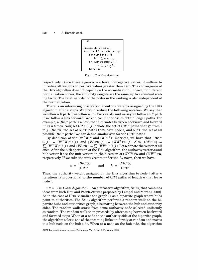
Kleinberg [1998] proposed the following iterative algorithm for computingthe hub and authority weights. Initially all authority and hub weights are setto 1. At each iteration, the operations O (“out”) and I (“in”) are performed.The O operation updates the authority weights, and the I operation updatesthe hub weights, both using Equation 1. A normalization step is then applied,so that the vectors a and h become unit vectors in some norm. The algorithmiterates until the vectors converge. This idea was later implemented as theHITS (Hyperlink Induced Topic Distillation) algorithm [Gibson et al. 1998]. Thealgorithm is summarized in Figure 1.
Kleinberg [1998] proves that the algorithm computes the principal left andright singular vectors of the adjacency matrix W . That is, the vectors a and hconverge to the principal right eigenvectors of the matrices MH = W T W andM T
H = WWT , respectively. The convergence of HITS to the singular vectors ofmatrix W is subject to the condition that the initial authority and hub vec-tors are not orthogonal to the principal eigenvectors of matrices MH and M T
H ,
ACM Transactions on Internet Technology, Vol. 5, No. 1, February 2005.
236 • A. Borodin et al.
Fig. 1. The HITS algorithm.
respectively. Since these eigenvectors have nonnegative values, it suffices toinitialize all weights to positive values greater than zero. The convergence ofthe HITS algorithm does not depend on the normalization. Indeed, for differentnormalization norms, the authority weights are the same, up to a constant scal-ing factor. The relative order of the nodes in the ranking is also independent ofthe normalization.
There is an interesting observation about the weights assigned by the HITS
algorithm after n steps. We first introduce the following notation. We say thatwe follow a B path if we follow a link backwards, and we say we follow an F pathif we follow a link forward. We can combine these to obtain longer paths. Forexample, a (BF)n path is a path that alternates between backward and forwardlinks n times. Now, let (BF)n(i, j ) denote the set of (BF)n paths that go from ito j , (BF)n(i) the set of (BF)n paths that leave node i, and (BF)n the set of allpossible (BF)n paths. We can define similar sets for the (FB)n paths.
By definition of the (W T W )n and (W W T )n matrices, we have that |(BF)n
(i, j )| = (W T W )n(i, j ), and |(FB)n(i, j )| = (WWT )n(i, j ). Also, |(BF)n(i)| =∑j (W
T W )n(i, j ), and |(FB)n(i)| = ∑j (WWT )n(i, j ). Let udenote the vector of all
ones. After the n-th operation of the HITS algorithm, the authority vector aandhub vector h are the unit vectors in the direction of (W T W )nu and (W W T )nu,respectively. If we take the unit vectors under the L1 norm, then we have
ai = |(BF)n(i)||(BF)n| and hi = |(FB)n(i)|
|(FB)n| .
Thus, the authority weight assigned by the HITS algorithm to node i after niterations is proportional to the number of (BF) paths of length n that leavenode i.
2.2.4 The SALSA Algorithm. An alternative algorithm, SALSA, that combinesideas from both HITS and PAGERANK was proposed by Lempel and Moran [2000].As in the case of HITS, visualize the graph G as a bipartite graph where hubspoint to authorities. The SALSA algorithm performs a random walk on the bi-partite hubs and authorities graph, alternating between the hub and authoritysides. The random walk starts from some authority node selected uniformlyat random. The random walk then proceeds by alternating between backwardand forward steps. When at a node on the authority side of the bipartite graph,the algorithm selects one of the incoming links uniformly at random and movesto a hub node on the hub side. When at a node on the hub side, the algorithm
ACM Transactions on Internet Technology, Vol. 5, No. 1, February 2005.

Link Analysis Ranking: Algorithms, Theory and Experiments • 237
selects one of the outgoing links uniformly at random and moves to an author-ity. The authority weights are defined to be the stationary distribution of thisrandom walk. Formally, the Markov Chain of the random walk has transitionprobabilities
Pa(i, j ) =∑
k : k∈B(i)∩B( j )
1|B(i)|
1|F (k)| .
Recall that Ga = (A, Ea) denotes the authority graph where there is an (undi-rected) edge between two authorities if they share a hub. This Markov Chaincorresponds to a random walk on the authority graph Ga where we move fromauthority i to authority j with probability Pa(i, j ). Let Wr denote the matrixderived from matrix W by normalizing the entries such that, for each row, thesum of the entries is 1, and let Wc denote the matrix derived from matrix Wby normalizing the entries such that, for each column, the sum of the entries is1. Then the stationary distribution of the SALSA algorithm is the principal lefteigenvector of the matrix MS = W T
c Wr .If the underlying authority graph Ga consists of more than one component,
then the SALSA algorithm selects a starting point uniformly at random and per-forms a random walk within the connected component that contains that node.Let j be a component that contains node i, let Aj denote the set of authoritiesin the component j , and E j the set of links in component j . Then the weightof authority i in component j is
ai = |Aj ||A|
|B(i)||E j | .
If the graph Ga consists of a single component (we refer to such graphs as au-thority connected graphs), that is, the underlying Markov Chain is irreducible,then the algorithm reduces to the INDEGREE algorithm. Furthermore, even whenthe graph Ga is not connected, if the starting point of the random walk is se-lected with probability proportional to the “popularity” (in-degree) of the nodein the graph G, then the algorithm again reduces to the INDEGREE algorithm.This algorithm was referred to as PSALSA (popularity-SALSA) by Borodin et al.[2001].
The SALSA algorithm can be thought of as a variation of the HITS algorithm.In the I operation of the HITS algorithm, the hubs broadcast their weights tothe authorities and the authorities sum up the weight of the hubs that point tothem. The SALSA algorithm modifies the I operation so that, instead of broad-casting, each hub divides its weight equally among the authorities to whichit points. Similarly, the SALSA algorithm modifies the O operation so that eachauthority divides its weight equally among the hubs that point to it. Therefore,
ai =∑
j : j∈B(i)
1|F ( j )|h j and hi =
∑j : j∈F (i)
1|B( j )|aj .
However, the SALSA algorithm does not really have the same “mutually reinforc-ing structure” that Kleinberg’s [1998] algorithm does. Indeed, ai = |Aj |
|A||B(i)||E j | ,
the relative authority of page i within a connected component is determinedfrom local links, not from the structure of the component.
ACM Transactions on Internet Technology, Vol. 5, No. 1, February 2005.

238 • A. Borodin et al.
Lempel and Moran [2000] define a similar Markov Chain for the hubs anda hub weight vector that is the stationary distribution of the correspondingrandom walk. The stationary distribution h is the left eigenvector of the matrixW T
r Wc.
2.2.5 Other Related Work. The ground-breaking work of Kleinberg [1998,1999], and Brin and Page [1998] was followed by a number of extensions andmodifications. Bharat and Henzinger [1998] and Chakrabarti et al. [1998] con-sider improvements on the HITS algorithm by using textual information toweight the importance of nodes and links. [Rafiei and Mendelzon 2000; Mendel-zon and Rafiei 2000] consider a variation of the HITS algorithm that uses ran-dom jumps, similar to SALSA. The same algorithm is also considered by Ng et al.[2001a, 2001b], termed Randomized HITS. Extensions of the HITS algorithmthat use multiple eigenvectors were proposed by Ng et al. [2001b] and Achliop-tas et al. [2001]. Tomlin [2003] proposes a generalization of the PAGERANK
algorithm that computes flow values for the edges of the Web graph, and aTrafficRank value for each page. A large body of work also exists that dealswith personalization of the PAGERANK algorithm [Page et al. 1998; Haveliwala2002; Jen and Widom 2003; Richardson and Domingos 2002].
A different line of research exploits the application of probabilistic and sta-tistical techniques for computing rankings. The PHITS algorithm by Cohn andChang [2000] assumes a probabilistic model in which a link is caused by latent“factors” or “topics”. They use the Expectation Maximization (EM) Algorithmof Dempster et al. [1977] to compute the authority weights of the pages. Theirwork is based on the Probabilistic Latent Semantic Analysis framework intro-duced by Hofmann [1999], who proposed a probabilistic alternative to SingularValue Decomposition. Hofmann [2000] proposes an algorithm similar to PHITS
which also takes into account the text of the documents. These algorithms re-quire specifying in advance the number of factors. Furthermore, it is possiblethat the EM Algorithm gets “stuck” in a local maximum, without converging tothe true global maximum.
3. NEW LINK ANALYSIS RANKING ALGORITHMS
The idea underlying the HITS algorithm can be captured in the following recur-sive definition of quality: “A good authority is one that is pointed to by many goodhubs, and a good hub is one that points to many good authorities”. Therefore,the quality of some page p as an authority (captured by the authority weight ofpage p) depends on the quality of the pages that point to p as hubs (capturedin the hub weight of the pages), and vice versa. Kleinberg [1998] proposes toassociate the hub and authority weights through the addition operation. Theauthority weight of a page p is defined to be the sum of the hub weights of thepages that point to p, and the hub weight of the page p is defined to be the sumof the authority weights of the pages that are pointed to by p. This definition hasthe following two implicit properties. First, it is symmetric in the sense that bothhub and authority weights are defined in the same way. If we reverse the orien-tation of the edges in the graph G, then authority and hub weights are swapped.Second, it is egalitarian in the sense that, when computing the hub weight of
ACM Transactions on Internet Technology, Vol. 5, No. 1, February 2005.
Link Analysis Ranking: Algorithms, Theory and Experiments • 239
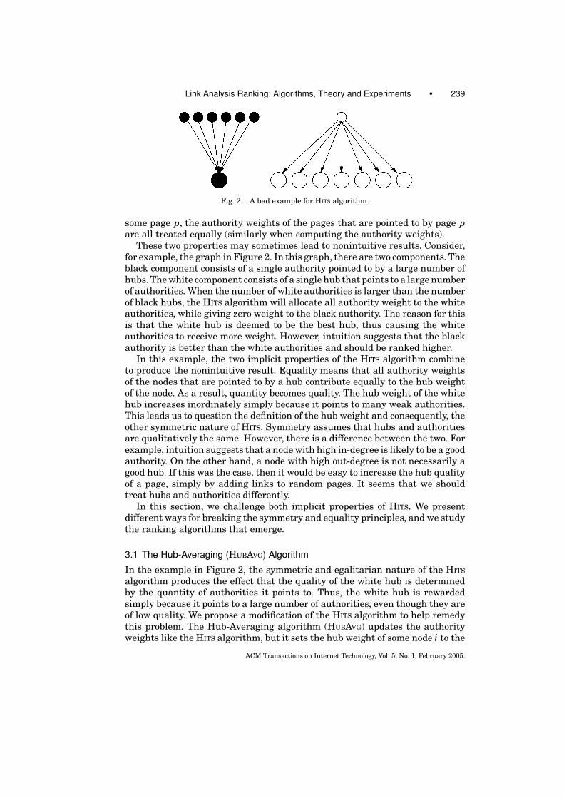
Fig. 2. A bad example for HITS algorithm.
some page p, the authority weights of the pages that are pointed to by page pare all treated equally (similarly when computing the authority weights).
These two properties may sometimes lead to nonintuitive results. Consider,for example, the graph in Figure 2. In this graph, there are two components. Theblack component consists of a single authority pointed to by a large number ofhubs. The white component consists of a single hub that points to a large numberof authorities. When the number of white authorities is larger than the numberof black hubs, the HITS algorithm will allocate all authority weight to the whiteauthorities, while giving zero weight to the black authority. The reason for thisis that the white hub is deemed to be the best hub, thus causing the whiteauthorities to receive more weight. However, intuition suggests that the blackauthority is better than the white authorities and should be ranked higher.
In this example, the two implicit properties of the HITS algorithm combineto produce the nonintuitive result. Equality means that all authority weightsof the nodes that are pointed to by a hub contribute equally to the hub weightof the node. As a result, quantity becomes quality. The hub weight of the whitehub increases inordinately simply because it points to many weak authorities.This leads us to question the definition of the hub weight and consequently, theother symmetric nature of HITS. Symmetry assumes that hubs and authoritiesare qualitatively the same. However, there is a difference between the two. Forexample, intuition suggests that a node with high in-degree is likely to be a goodauthority. On the other hand, a node with high out-degree is not necessarily agood hub. If this was the case, then it would be easy to increase the hub qualityof a page, simply by adding links to random pages. It seems that we shouldtreat hubs and authorities differently.
In this section, we challenge both implicit properties of HITS. We presentdifferent ways for breaking the symmetry and equality principles, and we studythe ranking algorithms that emerge.
3.1 The Hub-Averaging (HUBAVG) Algorithm
In the example in Figure 2, the symmetric and egalitarian nature of the HITS
algorithm produces the effect that the quality of the white hub is determinedby the quantity of authorities it points to. Thus, the white hub is rewardedsimply because it points to a large number of authorities, even though they areof low quality. We propose a modification of the HITS algorithm to help remedythis problem. The Hub-Averaging algorithm (HUBAVG) updates the authorityweights like the HITS algorithm, but it sets the hub weight of some node i to the
ACM Transactions on Internet Technology, Vol. 5, No. 1, February 2005.

240 • A. Borodin et al.
Fig. 3. The HUBAVG algorithm.
average authority weight of the authorities pointed to by hub i. Thus, for somenode i, we have
ai =∑
j∈B(i)
h j and hi = 1|F (i)|
∑j∈F (i)
aj . (2)
The intuition of the HUBAVG algorithm is that a good hub should point only (or atleast mainly) to good authorities, rather than to both good and bad authorities.Note that in the example in Figure 2, HUBAVG assigns the same weight to bothblack and white hubs, and it identifies the black authority as the best authority.The HUBAVG algorithm is summarized in Figure 3.
The HUBAVG algorithm can be viewed as a “hybrid” of the HITS and SALSA
algorithms. The operation of averaging the weights of the authorities pointedto by a hub is equivalent to dividing the weight of a hub among the authoritiesit points to. Therefore, the HUBAVG algorithm performs the O operation likethe HITS algorithm (broadcasting the authority weights to the hubs), and the Ioperation like the SALSA algorithm (dividing the hub weights to the authorities).This lack of symmetry between the update of hubs and authorities is motivatedby the qualitative difference between hubs and authorities discussed previously.The authority weights for the HUBAVG algorithm converge to the principal righteigenvector of the matrix MHA = W T Wr .
There is an interesting connection between HUBAVG and the Singular ValueDecomposition. Note that the matrix MHA can be expressed as MHA = W T F W ,where F is a diagonal matrix with F [i, i] = 1/|F (i)|. We also have that
MHA = (F 1/2W )T (F 1/2W ),
where F 1/2 is the square root of matrix F , that is, F [i, i] = 1/√
|F (i)|. Let W (i)denote the row vector that corresponds to the ith row of matrix W . Given thatall entries of the matrix W take 0/1 values, we have that ‖W (i)‖2 =
√|F (i)|.
Thus, the matrix F 1/2W is the matrix W , where each row is normalized to bea unit vector in the Euclidean norm. Let We denote this matrix. The hub andauthority vectors computed by the HUBAVG algorithm are the principal left andright singular vectors of the matrix We.
3.2 The Authority Threshold (AT(k)) Family of Algorithms
The HUBAVG algorithm has its own shortcomings. Consider, for example, thegraph in Figure 4. In this graph, there are again two components, one black
ACM Transactions on Internet Technology, Vol. 5, No. 1, February 2005.
Link Analysis Ranking: Algorithms, Theory and Experiments • 241
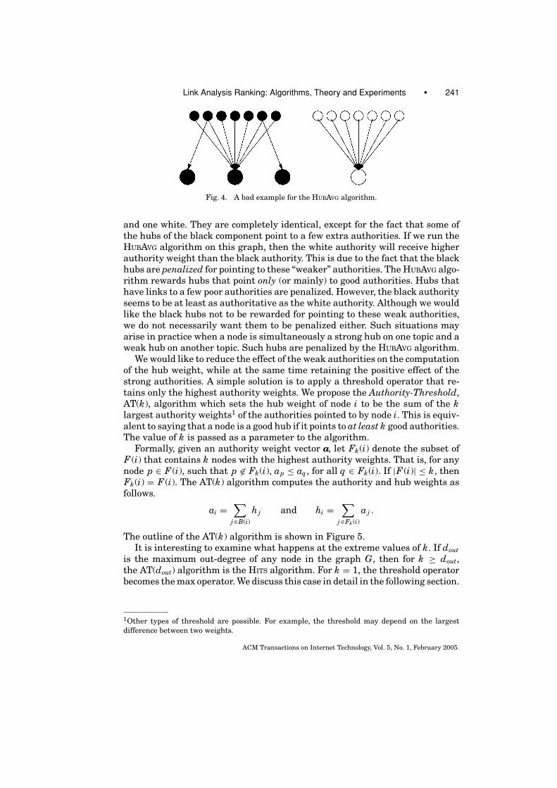
Fig. 4. A bad example for the HUBAVG algorithm.
and one white. They are completely identical, except for the fact that some ofthe hubs of the black component point to a few extra authorities. If we run theHUBAVG algorithm on this graph, then the white authority will receive higherauthority weight than the black authority. This is due to the fact that the blackhubs are penalized for pointing to these “weaker” authorities. The HUBAVG algo-rithm rewards hubs that point only (or mainly) to good authorities. Hubs thathave links to a few poor authorities are penalized. However, the black authorityseems to be at least as authoritative as the white authority. Although we wouldlike the black hubs not to be rewarded for pointing to these weak authorities,we do not necessarily want them to be penalized either. Such situations mayarise in practice when a node is simultaneously a strong hub on one topic and aweak hub on another topic. Such hubs are penalized by the HUBAVG algorithm.
We would like to reduce the effect of the weak authorities on the computationof the hub weight, while at the same time retaining the positive effect of thestrong authorities. A simple solution is to apply a threshold operator that re-tains only the highest authority weights. We propose the Authority-Threshold,AT(k), algorithm which sets the hub weight of node i to be the sum of the klargest authority weights1 of the authorities pointed to by node i. This is equiv-alent to saying that a node is a good hub if it points to at least k good authorities.The value of k is passed as a parameter to the algorithm.
Formally, given an authority weight vector a, let Fk(i) denote the subset ofF (i) that contains k nodes with the highest authority weights. That is, for anynode p ∈ F (i), such that p �∈ Fk(i), ap ≤ aq , for all q ∈ Fk(i). If |F (i)| ≤ k, thenFk(i) = F (i). The AT(k) algorithm computes the authority and hub weights asfollows.
ai =∑
j∈B(i)
h j and hi =∑
j∈Fk (i)
aj .
The outline of the AT(k) algorithm is shown in Figure 5.It is interesting to examine what happens at the extreme values of k. If dout
is the maximum out-degree of any node in the graph G, then for k ≥ dout,the AT(dout) algorithm is the HITS algorithm. For k = 1, the threshold operatorbecomes the max operator. We discuss this case in detail in the following section.
1Other types of threshold are possible. For example, the threshold may depend on the largestdifference between two weights.
ACM Transactions on Internet Technology, Vol. 5, No. 1, February 2005.

242 • A. Borodin et al.
Fig. 5. The AT(k) algorithm.
3.3 The MAX Algorithm
The MAX algorithm is a special case of the AT(k) algorithm for the thresholdvalue k = 1. The underlying intuition is that a hub node is as good as the bestauthority that it points to. That is, a good hub is one that points to at least onegood authority.
The MAX algorithm has some interesting properties. First, it is not hardto see that the nodes that receive the highest weight are the nodes with thehighest in-degree. We refer to these nodes as the seed nodes of the graph. Letd be the in-degree of the seed nodes. If we normalize in the L∞ norm, thenthe normalization factor for the authority weights of the MAX algorithm is d .The seed nodes receives weight 1, the maximum weight. A detailed analysisshows that the rest of the nodes are ranked according to their relation to theseed nodes. The convergence and the combinatorial properties of the stationaryweights of the MAX algorithm are discussed in detail in Tsaparas [2004b]. Inthe following paragraphs, we provide some of the intuition.
Let f : H → A denote a mapping between hubs and authorities, wherethe hub j is mapped to authority i, if authority i is the authority with themaximum weight among all the authorities pointed to by hub j . Define H(i) ={ j ∈ H : f ( j ) = i} to be the set of hubs that are mapped to authority i.Recall that the authority graph Ga, defined in Section 2.1, is an undirectedgraph, where we place an edge between two authorities if they share a hub. Wenow derive the directed weighted graph G A = (A, EA) on the authority nodes A,from the authority graph Ga as follows. Let i and j be two nodes in A, such thatthere exists an edge (i, j ) in the graph Ga, and ai �= aj . Let B(i, j ) = B(i) ∩ B( j )denote the set of hubs that point to both authorities i and j . Without loss ofgenerality, assume that ai > aj . If H(i) ∩ B(i, j ) �= ∅, that is, there exists at leastone hub in B(i, j ) that is mapped to the authority i, then we place a directededge from i to j . The weight c(i, j ) of the edge (i, j ) is equal to the size of theset H(i) ∩ B(i, j ), that is, it is equal to the number of hubs in B(i, j ) that aremapped to i. The intuition of the directed edge (i, j ) is that there are c(i, j ) hubsthat propagate the weight of node i to node j . The graph G A captures the flowof authority weight between authorities.
Now, let N (i) denote the set of nodes in G A that point to node i. Also, letci = ∑
j∈N (i) c( j , i) denote the total weight of the edges that point to i in thegraph G A. This is the number of hubs in the graph G that point to i, but aremapped to some node with weight greater than i. The remaining di − ci hubs
ACM Transactions on Internet Technology, Vol. 5, No. 1, February 2005.

Link Analysis Ranking: Algorithms, Theory and Experiments • 243
(if any) are mapped to node i, or to some node with weight equal to the weightof i. We set bi = di − ci. The number bi is also equal to the size of the set H(i),the set of hubs that are mapped to node i when all ties are broken in favor ofnode i.
The graph G A is a DAG, thus it must have at least one source. We canprove that the sources of G A are the seed nodes of the graph G [Tsaparas2004b]. We have already argued that the seed nodes receive maximum weight1. Let s be some seed node, and let i denote a nonseed node. We define dist(s, i)to be the distance of the longest path in G A, from s to i. We define the distanceof node i, dist(i) = maxs∈S dist(s, i), to be the maximum distance from a seednode to i, over all seed nodes. We note that the distance is well defined, sincethe graph G A is a DAG. The following theorem gives a recursive formula forweight ai, given the weights of the nodes in N (i).
THEOREM 3.1. Given a graph G, let C1, C2, . . . Ck be the connected compo-nents of the graph Ga. For every component Ci, 1 ≤ i ≤ k, if component Ci doesnot contain a seed node, then ax = 0, for all x in Ci. If component Ci contains aseed node, then the weight of the seed node is 1, and for every nonseed node x inCi, we can recursively compute the weight of node x at distance � > 0, using theequation
ax = 1d − bx
∑j∈N (x)
c( j , x)aj ,
where for all j ∈ N (i), dist( j ) < �.
3.4 The Breadth-First-Search (BFS) Algorithm
In this section, we introduce a Link Analysis Ranking algorithm that combinesideas from both the INDEGREE and the HITS algorithms. The INDEGREE algorithmcomputes the authority weight of a page, taking into account only the popularityof this page within its immediate neighborhood and disregarding the rest of thegraph. On the other hand, the HITS algorithm considers the whole graph, takinginto account the structure of the graph around the node, rather than just thepopularity of that node in the graph.
We now describe the Breadth-First-Search (BFS) algorithm as a generaliza-tion of the INDEGREE algorithm inspired by the HITS algorithm. The BFS algo-rithm extends the idea of popularity that appears in the INDEGREE algorithmfrom a one-link neighborhood to an n-link neighborhood. The construction of then-link neighborhood is inspired by the HITS algorithm. Recall from Section 2.2.3that the weight assigned to node i by the HITS algorithm after n steps is pro-portional to the number of (BF ) paths of length n that leave node i. For theBFS algorithm, instead of considering the number of (BF)n paths that leave i,it considers the number of (BF)n neighbors of node i. Overloading the notation,let (BF)n(i) denote the set of nodes that can be reached from i by following a(BF)n path. The contribution of node j to the weight of node i depends on thedistance of the node j from i. We adopt an exponentially decreasing weighting
ACM Transactions on Internet Technology, Vol. 5, No. 1, February 2005.

244 • A. Borodin et al.
scheme. Therefore, the weight of node i is determined as follows:
ai = |B(i)| + 12
|BF(i)| + 122
|BFB(i)| + . . . + 122n−1
|(BF)n(i)|.The algorithm starts from node i, and visits its neighbors in BFS order,
alternating between backward and forward steps. Every time we move one linkfurther from the starting node i, we update the weight factors accordingly. Thealgorithm stops either when n links have been traversed, or when the nodesthat can be reached from node i are exhausted.
The idea of applying an exponentially decreasing weighting scheme to pathsthat originate from a node has been previously considered by Katz [1953]. Inthe algorithm of Katz, for some fixed parameter α < 1, the weight of node i isequal to
ai =∞∑
k=1
n∑j=1
αkW k[ j , i],
where W k is the kth power of the adjacency matrix W . The entry W k[ j , i] is thenumber of paths in the graph G of length k from node j to node i. As we movefurther away from node i, the contribution of the paths decreases exponentially.There are two important differences between BFS and the algorithm of Katz.First, the way the paths are constructed is different, since the BFS algorithmalternates between backward and forward steps. More important, the BFS al-gorithm considers the neighbors at distance k. Every node j contributes to theweight of node i just once, and the contribution of node j is 1/2k (or αk if weselect a different scaling factor), where k is the shortest path (which alternatesbetween B and F steps) from j to i. In the algorithm of Katz, the same nodej may contribute multiple times, and its contribution is the number of pathsthat connect j with i.
The BFS algorithm ranks the nodes according to their reachability, that is,the number of nodes reachable from each node. This property differentiates theBFS algorithm from the remaining algorithms, where connectivity, that is, thenumber of paths that leave each node, is the most important factor in the rank-ing of the nodes.
3.5 The BAYESIAN Algorithm
We now introduce a different type of algorithm that uses a fully Bayesian statis-tical approach to compute authority and hub weights. Let P be the set of nodesin the graph. We assume that each node i is associated with three parame-ters. An (unknown) real parameter ei, corresponding to its “general tendency tohave hypertext links”, an (unknown) nonnegative parameter hi, correspondingto its “tendency to have intelligent hypertext links to authoritative sites”, andan (unknown) nonnegative parameter ai corresponding to its level of authority.
Our statistical model is as follows. The a priori probability of a link fromnode i to node j is given by
P(i → j ) = exp(aj hi + ei)1 + exp(aj hi + ei)
, (3)
ACM Transactions on Internet Technology, Vol. 5, No. 1, February 2005.

Link Analysis Ranking: Algorithms, Theory and Experiments • 245
and the probability of no link from i to j given by
P(i �→ j ) = 11 + exp(aj hi + ei)
. (4)
This reflects the idea that a link is more likely if ei is large (in which case hub ihas a large tendency to link to any site), or if both hi and aj are large (in whichcase i is an intelligent hub, and j is a high-quality authority).
To complete the specification of the statistical model from a Bayesian point ofview (see, e.g., Bernardo and Smith [1994]), we must assign prior distributionsto the 3n unknown parameters ei, hi, and ai. These priors should be generaland uninformative, and should not depend on the observed data. For largegraphs, the choice of priors should have only a small impact on the results.We let µ = −5.0 and σ = 0.1 be fixed parameters, and let each ei have priordistribution N (µ, σ 2), a normal distribution with mean µ and variance σ 2. Wefurther let each hi and aj have prior distribution Exp(1) (since they have to benonnegative), meaning that for x ≥ 0, P(hi ≥ x) = P(aj ≥ x) = exp(−x).
The (standard) Bayesian inference method then proceeds from this fully-specified statistical model by conditioning on the observed data, which in thiscase is the matrix W of actual observed hypertext links in the Base Set.Specifically, when we condition on the data W we obtain a posterior densityπ : R
3n → [0, ∞) for the parameters (e1, . . . , en, h1, . . . , hn, a1, . . . , an). This den-sity is defined so that
P((e1, . . . , en, h1, . . . , hn, a1, . . . , an) ∈ S | {W [i, j ]})= ∫
S π (e1, . . . , en, h1, . . . , hn, a1, . . . , an)de1 . . . dendh1 . . . dhnda1 . . . dan (5)
for any (measurable) subset S ⊆ R3n, and also
E(g (e1, . . . , en, h1, . . . , hn, a1, . . . , an) | {W [i, j ]})= ∫
R3n g (e1, . . . , en, h1, . . . , hn, a1, . . . , an)π (e1, . . . , en, h1, . . . , hn, a1, . . . , an)de1 . . . dendh1 . . . dhnda1 . . . dan
for any (measurable) function g : R3n → R. An easy computation gives the
following.
LEMMA 3.2. For our model, the posterior density is given, up to a multiplica-tive constant, by
π (e1, . . . , en, h1, . . . , hn, a1, . . . , an)
∝n∏
i=1
exp(−hi) exp(−ai) exp[−(ei − µ)2/(2σ 2)]
×∏
(i, j ):W [i, j ]=1
exp(aj hi + ei)
/ ∏all i, j
(1 + exp(aj hi + ei)) .
ACM Transactions on Internet Technology, Vol. 5, No. 1, February 2005.

246 • A. Borodin et al.
PROOF. We compute that
P(e1 ∈ de1, . . . , en ∈ den, h1 ∈ dh1, . . . , hn ∈ dhn, a1 ∈ da1, . . . , an
∈ dan, {W [i, j ]}) =n∏
i=1
[P(ei ∈ dei)P(hi ∈ dhi)P(ai ∈ dai)]
×∏
i, j :W [i, j ]=1
P(W [i, j ] = 1 | ei, hi, aj )×∏
i, j :W [i, j ]=0
P(W [i, j ] = 0 | ei, hi, aj )
=n∏
i=1
[exp[−(ei − µ)2/(2σ 2)]dei exp(−hi)dhi exp(−ai)dai]
×∏
i, j :W [i, j ]=1
exp(aj hi + ei)1 + exp(aj hi + ei)
∏i, j :W [i, j ]=0
11 + exp(aj hi + ei)
=n∏
i=1
[exp[−(ei − µ)2/(2σ 2)]dei exp(−hi)dhi exp(−ai)dai]
×∏
i, j :W [i, j ]=1
exp(aj hi + ei)
/ ∏all i, j
(1 + exp(aj hi + ei)) .
The result now follows by inspection.
Our Bayesian algorithm then reports the conditional means of the 3n para-meters, according to the posterior density π . That is, it reports final values a j ,hi, and ei, where, for example,
a j =∫
R3na j π (e1, . . . , en, h1, . . . , hn, a1, . . . , an) de1 . . . dendh1 . . . dhnda1 . . . dan.
To actually compute these conditional means is nontrivial. To accomplishthis, we used a Metropolis Algorithm. The Metropolis algorithm is an exampleof a Markov Chain Monte Carlo Algorithm (for background see, e.g., Smithand Roberts [1993]; Tierney [1994]; Gilks et al. [1996]; Roberts and Rosenthal[1998]). We denote this algorithm as BAYESIAN.
The Metropolis Algorithm proceeds by starting all the 3n parameter values at1. It then attempts, for each parameter in turn, to add an independent N (0, ξ2)random variable to the parameter. It then “accepts” this new value with proba-bility min(1, π (new)/π (old )), otherwise it “rejects” it and leaves the parametervalue the way it is. If this algorithm is iterated enough times, and the observedparameter values at each iteration are averaged, then the resulting averageswill converge (see, e.g., Tierney [1994]) to the desired conditional means.
There is, of course, some arbitrariness in the specification of the BAYESIAN al-gorithm, for example, in the form of the prior distributions and in the precise for-mula for the probability of a link from i to j . However, the model appears to workwell in practice as our experiments show. We note that it is possible that thepriors for a new search query could instead depend on the performance of page ion different previous searches, though we do not pursue that direction here.
The BAYESIAN algorithm is similar in spirit to the PHITS algorithm of Cohn andChang [2000] in that both use statistical modeling, and both use an iterative
ACM Transactions on Internet Technology, Vol. 5, No. 1, February 2005.
Link Analysis Ranking: Algorithms, Theory and Experiments • 247
algorithm to converge to an answer. However, the algorithms differ sub-stantially in their details. First, they use substantially different statisticalmodels. Second, the PHITS algorithm uses a non-Bayesian (i.e., “classical” or“frequentist”) statistical framework, as opposed to the Bayesian frameworkadopted here.
3.6 The Simplified Bayesian (SBAYESIAN) Algorithm
It is possible to simplify the above Bayesian model by replacing equation (3)with
P(i → j ) = aj hi
1 + aj hi,
and correspondingly, replace equation (4) with
P(i �→ j ) = 11 + aj hi
.
This eliminates the parameters ei entirely so that we no longer need the priorvalues µ and σ . A similar model for the generation of links was considered byAzar et al. [2001].
This leads to a slightly modified posterior density π (·), now given by π :R
2n → R≥0 where
π (h1, . . . , hn, a1, . . . , an) ∝n∏
i=1
exp(−hi) exp(−ai) ×∏
(i, j ):W [i, j ]=1
aj hi
/∏all i, j
(1+aj hi).
We denote this Simplified Bayesian algorithm as SBAYESIAN. The SBAYESIAN
algorithm was designed to be to similar to the original BAYESIAN algorithm.Surprisingly, we observed that experimentally it performs very similarly to theINDEGREE algorithm.
4. A THEORETICAL FRAMEWORK FOR THE STUDY OF LINK ANALYSISRANKING ALGORITHMS
The seminal work of Kleinberg [1998] and Brin and Page [1998] was followed byan avalanche of Link Analysis Ranking algorithms (hereinafter denoted LARalgorithms) [Borodin et al. 2001; Bharat and Henzinger 1998; Lempel andMoran 2000; Rafiei and Mendelzon 2000; Azar et al. 2001; Achlioptas et al. 2001;Ng et al. 2001b]. Faced with this wide range of choices for LAR algorithms, re-searchers usually resort to experiments to evaluate them and determine whichone is more appropriate for the problem at hand. However, experiments are onlyindicative of the behavior of the LAR algorithm. In many cases, experimentalstudies are inconclusive. Furthermore, there are often cases where algorithmsexhibit similar properties and ranking behavior. For example, in our experi-ments (Section 5), we observed a strong “similarity” between the SBAYESIAN andINDEGREE algorithms.
It seems that experimental evaluation of the performance of an LAR al-gorithm is not sufficient to fully understand its ranking behavior. We need aprecise way to evaluate the properties of the LAR algorithms. We would like tobe able to formally answer questions of the following type: “How similar are two
ACM Transactions on Internet Technology, Vol. 5, No. 1, February 2005.

248 • A. Borodin et al.
LAR algorithms?”; “On what kind of graphs do two LAR algorithms return sim-ilar rankings?”; “How does the ranking behavior of an LAR algorithm dependon the specific class of graphs?”; “How does the ranking of an LAR algorithmchange as the underlying graph is modified?”; “Is there a set of properties thatcharacterize an LAR algorithm?”.
In this section we, describe a formal study of LAR algorithms. We introducea theoretical framework that allows us to define properties of the LAR algo-rithms and compare their ranking behavior. We conclude with an axiomaticcharacterization of the INDEGREE algorithm.
4.1 Link Analysis Ranking Algorithms
We first need to formally define a Link Analysis Ranking algorithm. Let Gndenote the set of all possible graphs of size n. The size of the graph is thenumber of nodes in the graph. Let Gn ⊆ Gn denote a collection of graphs in Gn.We define a link analysis algorithm A as a function A : Gn → R
n that maps agraph G ∈ Gn to an n-dimensional real vector. The vector A(G) is the authorityweight vector (or weight vector) produced by the algorithm A on graph G. Wewill refer to this vector as the LAR vector, or authority vector. The value of theentry A(G)[i] of the LAR vector A(G) denotes the authority weight assigned bythe algorithm A to the node i. We will use a (or often w) to denote the authorityweight vector of algorithm A. In this section, we will sometimes use a(i) insteadof ai to denote the authority weight of node i. All algorithms that we consider aredefined over Gn, the class of all possible graphs. We will also consider anotherclass of graphs, GAC
n , the class of authority connected graphs. Recall that a graphG is authority connected, if the corresponding authority graph Ga consists of asingle component.
We will assume that the weight vectorA(G) is normalized under some chosennorm. The choice of normalization affects the output of the algorithm, so wedistinguish between algorithms that use different norms. For any norm L, wedefine an L-algorithm A to be an algorithm where the weight vector of A isnormalized under L. That is, the algorithm maps the graphs in Gn onto the unitL-sphere. For the following, when not stated explicitly, we will assume that theweight vectors of the algorithms are normalized under the Lp norm for some1 ≤ p ≤ ∞.
4.2 Distance Measures Between LAR Vectors
We are interested in comparing different LAR algorithms as well as studyingthe ranking behavior of a specific LAR algorithm as we modify the underlyinggraph. To this end, we need to define a distance measure between the LAR vec-tors produced by the algorithms. Recall that an LAR algorithm A is a functionthat maps a graph G = (P, E) from a class of graphs Gn to an n-dimensionalauthority weight vector A(G). Let a1 and a2 be two LAR vectors defined overthe same set of nodes P . We define the distance between the LAR vectors a1and a2 as d (a1, a2), where d : R
n × Rn → R is some function that maps two real
n-dimensional vectors to a real number d (a1, a2). We now examine differentchoices for the function d .
ACM Transactions on Internet Technology, Vol. 5, No. 1, February 2005.
Link Analysis Ranking: Algorithms, Theory and Experiments • 249
4.2.1 Geometric Distance Measures. The first distance functions we con-sider capture the closeness of the actual weights assigned to every node. TheLAR vectors can be viewed as points in an n-dimensional space, thus we can usecommon geometric measures of distance. We consider the Manhattan distance,that is, the L1 distance of the two vectors. Let a1, a2 be two LAR vectors. Wedefine the d1 distance measure between a1 and a2 as follows
d1(a1, a2) = minγ1,γ2≥1
n∑i=1
|γ1a1(i) − γ2a2(i)|.
The constants γ1 and γ2 are meant to allow for an arbitrary scaling of the twovectors, thus eliminating large distances that are caused solely due to normal-ization factors. For example, let w = (1, 1, . . . , 1, 2) and v = (1, 1, . . . , 1) betwo LAR vectors before any normalization is applied. These two vectors ap-pear to be close. Suppose that we normalize the LAR vectors in the L∞ norm,and let w∞ and v∞ denote the normalized vectors. Then
∑ni=1 |w∞(i) − v∞(i)| =
(n−1)/2 = �(n). The maximum L1 distance between any two L∞-unit vectors is�(n) [Tsaparas 2004a] and therefore, these two vectors appear to be far apart.Suppose now that we normalize in the L1 norm, and let w1 and v1 denote thenormalized vectors. Then
∑ni=1 |w1(i) − v1(i)| = 2(n−1)
n(n+1) = �(1/n). The maximumL1 distance between any two L1-unit vectors is �(1); therefore, the two vectorsnow appear to be close. We use the constants γ1, γ2 to avoid such discrepancies.
Instead of the L1 distance, we may use other geometric distance measures,such as the Euclidean distance L2. In general, we define the dq distance, as theLq distance of the weight vectors. Formally,
dq(a1, a2) = minγ1,γ2≥1
‖γ1a1(i) − γ2a2(i)‖q .
For the remainder of the article, we only consider the d1 distance measure.
4.2.2 Rank Distance Measures. The next distance functions we considercapture the similarity between the ordinal rankings induced by the two LARvectors. The motivation behind this definition is that the ordinal ranking is theusual end-product seen by the user. Let abe an LAR vector defined over a set Pof n nodes. The vector a induces a ranking of the nodes in P , such that a nodei is ranked above node j if ai > aj . If all weights are distinct, the authorityweights induce a total ranking of the elements in P . If the weights are not alldistinct, then we have a partial ranking of the elements in P . We will also referto total rankings as permutations.
The problem of comparing permutations has been studied exten-sively [Kendall 1970; Diaconis and Graham 1977; Dwork et al. 2001]. One pop-ular distance measure is the Kendall’s tau distance which captures the numberof disagreements between the rankings. Let P denote the set of all pairs ofnodes. Let a1, a2 be two LAR vectors. We define the violating set, V(a1, a2) ⊆ P,as follows
V(a1, a2) = {(i, j ) inP : (a1(i) < a1( j )∧a2(i) > a2( j ))∨(a1(i) > a1( j )∧a2(i) < a2( j ))}.That is, the violating set contains the set of pairs of nodes that are ranked in adifferent order by the two permutations. We now define the indicator function
ACM Transactions on Internet Technology, Vol. 5, No. 1, February 2005.

250 • A. Borodin et al.
Ia1a2 (i, j ) as follows.
Ia1a2 (i, j ) ={
1 if (i, j ) ∈ V(a1, a2)0 otherwise
.
Kendall’s tau is defined as follows.
K (a1, a2) =∑
{i, j }∈PIa1a2 (i, j ).
Kendall’s tau is equal to the number of bubble sort swaps that are necessaryto convert one permutation to the other. The maximum value of Kendall’s tauis n(n − 1)/2, and it occurs when one ranking is the reverse of the other.
If the two LAR vectors take distinct values for each node in the set P , thenwe can compare rankings by directly applying Kendal’s tau distance. However,it is often the case that LAR algorithms assigns equal weights to two differentnodes. Thus, the algorithm produces a partial ranking of the nodes. In this case,there is an additional source of discrepancy between the two rankings; pairsof nodes that receive equal weight in one vector, but different weights in theother. We define the weakly violating set, W(a1, a2), as follows.
W(a1, a2) = {(i, j ) : (a1(i) = a1( j )∧a2(i) �= a2( j ))∨(a1(i) �= a1( j )∧a2(i) = a2( j ))}.In order to define a distance measure between partial rankings, we need to ad-dress the pairs of nodes that belong to this set. Following the approach in Faginet al. [2003], we penalize each such pair by a value p, where p ∈ [0, 1]. Wedefine the indicator function I (p)
a1a2(i, j ) as follows.
I pa1a2
(i, j ) =
1 if (i, j ) ∈ V(a1, a2)p if (i, j ) ∈ W(a1, a2).0 otherwise
Kendall’s tau with penalty p is defined as follows.
K (p)(a1, a2) =∑
{i, j }∈PI (p)a1a2
(i, j ).
The parameter p takes values in [0, 1]. The value p = 0 gives a lenient approachwhere we penalize the algorithm only for pairs that are weighted so that theyforce an inconsistent ranking. The value p = 1 gives a strict approach where wepenalize the algorithm for all pairs that are weighted so that they allow for aninconsistent ranking. Values of p in (0, 1) give a combined approach. We notethat K (0)(a1, a2) ≤ K (p)(a1, a2) ≤ K (1)(a1, a2).
In this article, we only consider the extreme values of p. We define the weakrank distance, d (0)
r , as follows.
d (0)r (a1, a2) = 1
n(n − 1)/2K (0)(a1a2).
We define the strict rank distance, d (1)r , as follows.
d (1)r (a1, a2) = 1
n(n − 1)/2K (1)(a1a2).
ACM Transactions on Internet Technology, Vol. 5, No. 1, February 2005.
Link Analysis Ranking: Algorithms, Theory and Experiments • 251
A p-rank distance d (p) can be defined similarly. The rank distance measuresare normalized by n(n−1)/2, the maximum Kendal’s tau distance, so that theytakes values in [0, 1]. We will use the weak rank distance when we want to argueabout two LAR vectors being far apart, and the strict rank distance when wewant to argue about two LAR vectors being close.
The problem of comparing partial rankings is studied independentlyin Tsaparas [2004a] and Fagin et al. [2004] where they discuss the properties ofKendal tau distance on partial rankings. It is shown that the d (1)
r distance mea-sure is a metric. Also, Fagin et al. [2004] generalize other distance measuresfor the case of partial rankings.
4.3 Similarity of LAR Algorithms
We now turn to the problem of comparing two LAR algorithms. We first give thefollowing generic definition of similarity of two LAR algorithms for any distancefunction d , and any normalization norm L = || · ||.
Definition 4.1. Two L-algorithms, A1 and A2, are similar on the class ofgraph Gn under distance d , if as n → ∞
maxG∈Gn
d (A1(G), A2(G)) = o(Mn(d , L))
where Mn(d , L) = sup‖w1‖=‖w2‖=1 d (w1, w2) is the maximum distance betweenany two n-dimensional vectors with unit norm L = || · ||.
In the definition of similarity, instead of taking the maximum over all G ∈ Gn,we may use some other operator. For example, if there exists some distributionover the graphs in Gn, we could replace max operator by the expectation ofthe distance between the algorithms. In this article, we only consider the maxoperator.
We now give the following definitions of similarity for the d1, d (0)r , and d (1)
rdistance measures. For the d1 distance measure, the maximum d1 distancebetween any two n-dimensional Lp unit vectors is �(n1−1/p) [Tsaparas 2004a].
Definition 4.2. Let 1 ≤ p ≤ ∞. Two Lp-algorithms, A1, and A2, are d1-similar (or, similar) on the class of graphs Gn, if as n → ∞,
maxG∈Gn
d1(A1(G), A2(G)) = o(n1−1/p).
Definition 4.3. Two algorithms, A1 and A2, are weakly rank similar on theclass of graphs Gn, if as n → ∞,
maxG∈Gn
d (0)r (A1(G), A2(G)) = o(1).
Definition 4.4. Two algorithms, A1 and A2, are strictly rank similar on theclass of graphs Gn, if as n → ∞,
maxG∈Gn
d (1)r (A1(G), A2(G)) = o(1).
ACM Transactions on Internet Technology, Vol. 5, No. 1, February 2005.
252 • A. Borodin et al.
Definition 4.5. Two algorithms, A1 and A2, are rank consistent on the classof graphs Gn, if for every graph G ∈ Gn,
d (0)r (A1(G), A2(G)) = 0.
Definition 4.6. Two algorithms, A1 and A2, are rank equivalent on the classof graphs Gn, if for every graph G ∈ Gn,
d (1)r (A1(G), A2(G)) = 0.
We note that, according to the above definition, every algorithm is rank con-sistent with the trivial algorithm that gives the same weight to all authorities.Although this may seem somewhat bizarre, it does have an intuitive justifica-tion. For an algorithm whose goal is to produce an ordinal ranking, the weightvector with all weights equal conveys no information; therefore, it lends itselfto all possible ordinal rankings. The weak rank distance counts only the pairsthat are weighted inconsistently, and in this case there are none. If a strongernotion of similarity is needed, the d (1)
r distance measure can be used where allsuch pairs contribute to the distance.
From the definitions in Section 4.2.2, it is obvious that if two algorithms arestrictly rank similar, then they are similar under p-rank distance d (p)
r for everyp < 1. Equivalently, if two algorithms are not weakly rank similar, then theyare not similar under p-rank distance for every p > 0.
The definition of similarity depends on the normalization of the algorithms.In the following, we show that, for the d1 distance, similarity in the Lp normimplies similarity in the Lq norm, for any q > p.
THEOREM 4.7. Let A1 and A2 be two algorithms, and let 1 ≤ p ≤ q ≤ ∞. Ifthe Lp-algorithmA1 and the Lp-algorithmA2 are similar, then the Lq-algorithmA1 and the Lq-algorithm A2 are also similar.
PROOF. Let G be a graph of size n, and let u = A1(G), and v = A2(G)be the weight vectors of the two algorithms. Let vp and up denote the weightvectors, normalized in the Lp norm, and let vq and uq denote the weight vectors,normalized in the Lq norm. Since the Lp-algorithm A1 and the Lp-algorithmA2 are similar, there exist γ1, γ2 ≥ 1 such that
d1(vp, up) =n∑
i=1
|γ1vp(i) − γ2up(i)| = o(n1−1/p).
Now, vq = vp/‖vp‖q , and uq = up/‖up‖q . Therefore,∑n
i=1 |γ1‖vp‖qvq(i) −γ2‖up‖quq(i)| = o(n1−1/p). Without loss of generality, assume that ‖up‖q ≥ ‖vp‖q .Then
‖vp‖q
n∑i=1
∣∣∣∣γ1vq(i) − γ2‖up‖q
‖vp‖quq(i)
∣∣∣∣ = o(n1−1/p).
We set γ ′1 = γ1 and γ ′
2 = γ2‖up‖q
‖vp‖q. Then we have that
d1(vq , uq) ≤n∑
i=1
|γ ′1vq(i) − γ ′
2uq(i)| = o(
n1−1/p
‖vp‖q
).
ACM Transactions on Internet Technology, Vol. 5, No. 1, February 2005.
Link Analysis Ranking: Algorithms, Theory and Experiments • 253
Fig. 6. Dissimilarity of HITS and INDEGREE. The graph G for r = 2.
It is known [Tsaparas 2004a] that ‖vp‖q ≥ ‖vp‖pn1/q−1/p = n1/q−1/p. Hence,n1−1/p
‖vp‖q≤ n1−1/p
n1/q−1/p = n1−1/q . Therefore, d1(vq , uq) = o(n1−1/q), and thus Lq-algorithmA1, and Lq-algorithm A2 are similar.
Theorem 4.7 implies that if two L1-algorithms are similar, then the corre-sponding Lp-algorithms are also similar, for any 1 ≤ p ≤ ∞. Consequently, iftwo L∞-algorithms are dissimilar, then the corresponding Lp-algorithms arealso dissimilar, for any 1 ≤ p ≤ ∞. Therefore, all dissimilarity results provenfor the L∞ norm hold for any Lp norm, for 1 ≤ p ≤ ∞.
4.3.1 Similarity Results. We now consider the similarity of the HITS, IN-DEGREE, SALSA, HUBAVG, and MAX algorithms. We will show that no pair of algo-rithms are similar, or rank similar, in the class Gn of all possible graphs of sizen. For the dissimilarity results under the d1 distance measure, we will assumethat the weight vectors are normalized under the L∞ norm. Dissimilarity be-tween two L∞-algorithms implies dissimilarity in Lp norm, for p < ∞. Also,for rank similarity, we will use the strict rank distance, d (1)
r , while for rankdissimilarity we will use the weak rank distance, d (0)
r .
4.3.1.1 The HITS and the INDEGREE Algorithms.
PROPOSITION 4.8. The HITS and the INDEGREE algorithms are neither similar,nor weakly rank similar on Gn.
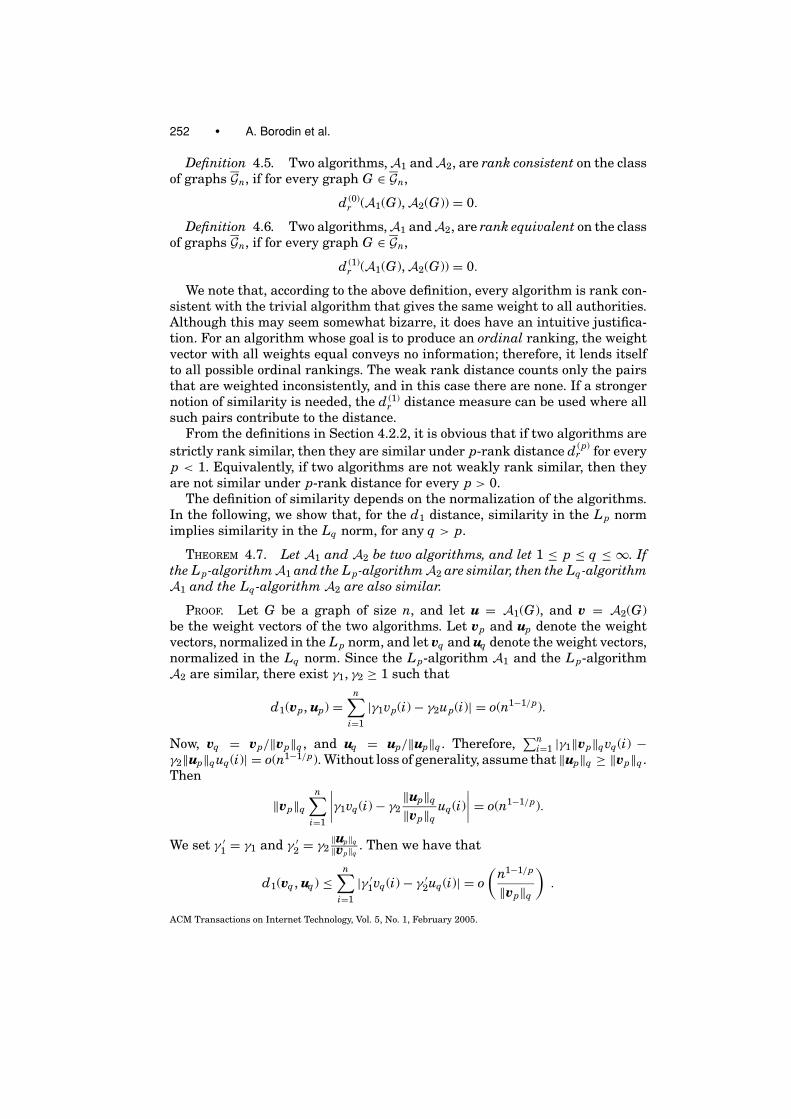
PROOF. Consider a graph G on n = 7r − 2 nodes that consists of two dis-connected components. The first component C1 consists of a complete bipartitegraph with 2r−1 hubs and 2r−1 authorities. The second component C2 consistsof a bipartite graph with 2r hubs and r authorities. The graph G for r = 2 isshown in Figure 6.
Let aand wdenote the weight vectors of the HITS and the INDEGREE algorithm,respectively, on graph G. The HITS algorithm allocates all the weight to thenodes in C1. After normalization, for all i ∈ C1, ai = 1, while for all j ∈ C2, aj =0. On the other hand, the INDEGREE algorithm distributes the weight to bothcomponents, allocating more weight to the nodes in C2. After the normalizationstep, for all j ∈ C2, wj = 1, while for all i ∈ C1, wi = 2r−1
2r .There are r nodes in C2 for which wi = 1 and ai = 0. For all γ1, γ2 ≥ 1,∑i∈C2
|γ1wi − γ2ai| ≥ r. Therefore, d1(w, a) = (r) = (n), which proves thatthe algorithms are not similar.
ACM Transactions on Internet Technology, Vol. 5, No. 1, February 2005.

254 • A. Borodin et al.
Fig. 7. Dissimilarity of HUBAVG and HITS. The graph G for r = 3.
The proof for weak rank dissimilarity follows immediately from the above.For every pair of nodes {i, j } such that i ∈ C1 and j ∈ C2, ai > aj and wi < wj .There are �(n2) such pairs, therefore, d (0)
r (a, w) = �(1). Thus, the two algo-rithms are not weakly rank similar.
4.3.1.2 The HUBAVG and HITS Algorithms.
PROPOSITION 4.9. The HUBAVG and HITS algorithms are neither similar, norweakly rank similar on Gn.
PROOF. Consider a graph G on n = 5r nodes that consists of two disconnectedcomponents. The first component C1 consists of a complete bipartite graph withr hub and r authority nodes. The second component C2 consists of a completebipartite graph C with r hub and r authority nodes, and a set of r “external”authority nodes E, such that each hub node in C points to a node in E, andno two hub nodes in C point to the same “external” node. Figure 7 shows thegraph G for r = 3.
Let aand w denote the weight vectors of the HITS and the HUBAVG algorithm,respectively, on graph G. It is not hard to see that the HITS algorithm allocatesall the weight to the authority nodes in C2. After normalization, for all authoritynodes i ∈ C, ai = 1, for all j ∈ E, aj = 1
r−1 , and for all k ∈ C1, ak = 0. On theother hand, the HUBAVG algorithm allocates all the weight to the nodes in C1.After normalization, for all authority nodes k ∈ C1, wk = 1, and for all j ∈ C2,wj = 0.
Let U = C1 ∪ C. The set U contains 2r authority nodes. For every authorityi ∈ U , either ai = 1 and wi = 0, or ai = 0 and wi = 1. Therefore, for all γ1, γ2 ≥ 1,∑
i∈U |γ1ai − γ2wi| ≥ 2r. Thus, d1(a, w) = (r) = (n), which proves that thealgorithms are not similar.
The proof for weak rank dissimilarity follows immediately from the above.For every pair of authority nodes (i, j ) such that i ∈ C1 and j ∈ C2, ai < wj ,and ai > wj . There are �(n2) such pairs, therefore, d (0)
r (a, w) = �(1). Thus, thetwo algorithms are not weakly rank similar.
4.3.1.3 The HUBAVG and INDEGREE Algorithms.
PROPOSITION 4.10. The HUBAVG algorithm and the INDEGREE algorithm areneither similar, nor weakly rank similar on Gn.
PROOF. Consider a graph G with n = 15r nodes. The graph G consists of rcopies of a subgraph Gs on 15 nodes. The subgraph Gs contains two components,
ACM Transactions on Internet Technology, Vol. 5, No. 1, February 2005.
Link Analysis Ranking: Algorithms, Theory and Experiments • 255
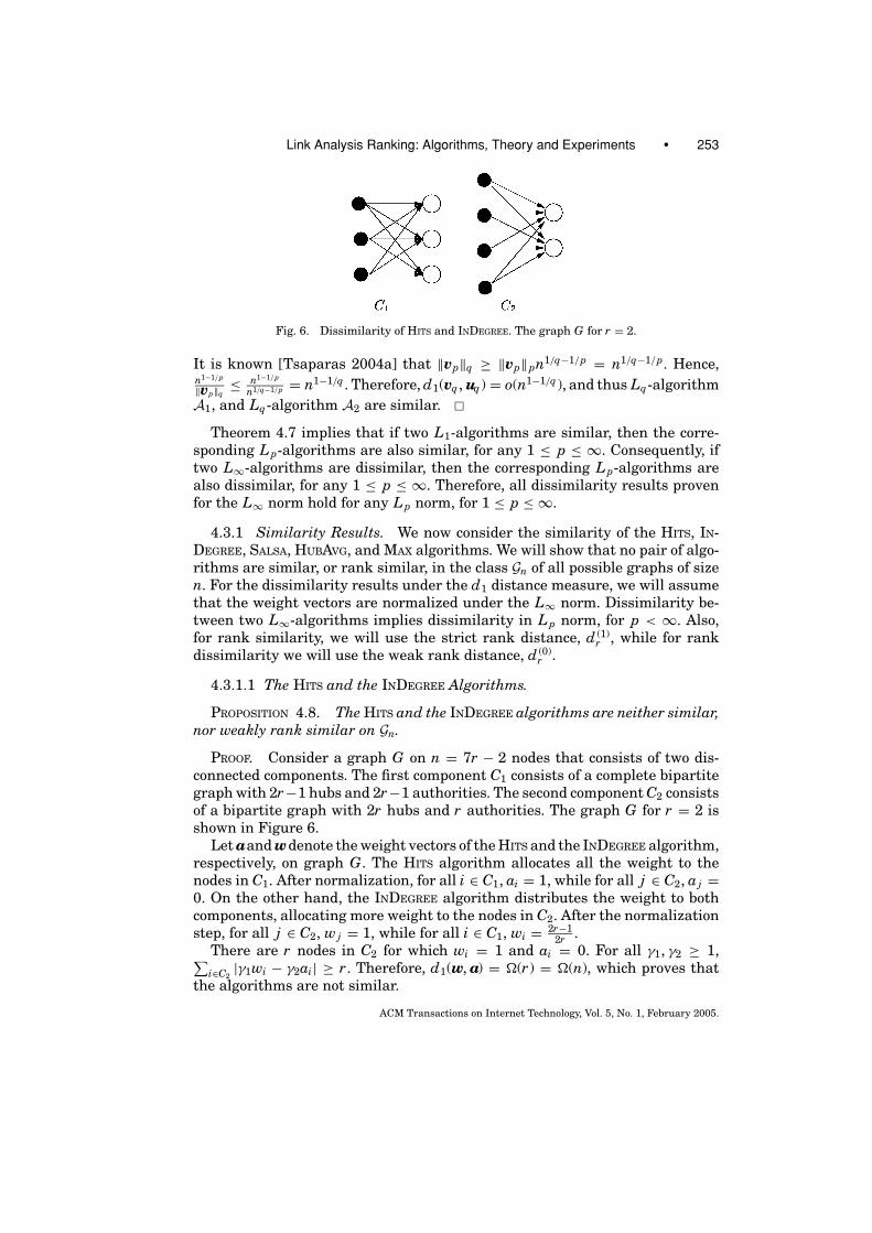
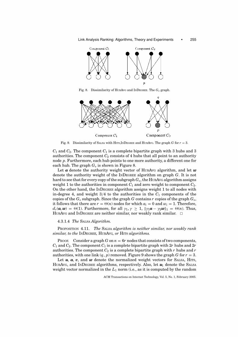
Fig. 8. Dissimilarity of HUBAVG and INDEGREE. The Gs graph.
Fig. 9. Dissimilarity of SALSA with HITS,INDEGREE and HUBAVG. The graph G for r = 3.
C1 and C2. The component C1 is a complete bipartite graph with 3 hubs and 3authorities. The component C2 consists of 4 hubs that all point to an authoritynode p. Furthermore, each hub points to one more authority, a different one foreach hub. The graph Gs is shown in Figure 8.
Let a denote the authority weight vector of HUBAVG algorithm, and let wdenote the authority weight of the INDEGREE algorithm on graph G. It is nothard to see that for every copy of the subgraph Gs, the HUBAVG algorithm assignsweight 1 to the authorities in component C1 and zero weight to component C2.On the other hand, the INDEGREE algorithm assigns weight 1 to all nodes within-degree 4, and weight 3/4 to the authorities in the C1 components of thecopies of the Gs subgraph. Since the graph G contains r copies of the graph Gs,it follows that there are r = �(n) nodes for which ai = 0 and wi = 1. Therefore,dr (a, w) = �(1). Furthermore, for all γ1, γ ≥ 1, ‖γ1a − γ2w‖1 = �(n). Thus,HUBAVG and INDEGREE are neither similar, nor weakly rank similar.
4.3.1.4 The SALSA Algorithm.
PROPOSITION 4.11. The SALSA algorithm is neither similar, nor weakly ranksimilar, to the INDEGREE, HUBAVG, or HITS algorithms.
PROOF. Consider a graph G on n = 6r nodes that consists of two components,C1 and C2. The component C1 is a complete bipartite graph with 2r hubs and 2rauthorities. The component C2 is a complete bipartite graph with r hubs and rauthorities, with one link (q, p) removed. Figure 9 shows the graph G for r = 3.
Let u, a, v, and w denote the normalized weight vectors for SALSA, HITS,HUBAVG, and INDEGREE algorithms, respectively. Also, let u1 denote the SALSA
weight vector normalized in the L1 norm (i.e., as it is computed by the random
ACM Transactions on Internet Technology, Vol. 5, No. 1, February 2005.

256 • A. Borodin et al.
walk of the SALSA algorithm). The SALSA algorithm allocates weight u1(i) = 1/3rfor all authority nodes i ∈ C1, and weight u1( j ) = (r − 1)/3(r2 − 1) for allauthority node j ∈ C2 \ {p}. Hub nodes receive weight zero for all algorithms. Itis interesting to note that the removal of the link (q, p) increases the weight ofthe rest of the nodes in C2. Since (r −1)/3(r2 −1) > 1/3r, after normalization inthe L∞ norm, we have that ui = 1− 1
r2 for all i ∈ C1, and u j = 1 for all j ∈ C2\{p}.On the other hand, both the HITS and HUBAVG algorithms distribute all theweight equally to the authorities in the C1 component and allocate zero weightto the nodes in the C2 component. Therefore, after normalization, ai = vi = 1 forall nodes i ∈ C1, and aj = vj = 0 for all nodes j ∈ C2. The INDEGREE algorithmallocates weight proportionally to the in-degree of the nodes, therefore, afternormalization, wi = 1 for all nodes in C1, while wj = 1
2 for all nodes j ∈ C2 \{p}.Let ‖ · ‖ denote the L1 norm. For the HITS and HUBAVG algorithm, there are
r entries in C2 \ {p}, for which ai = vi = 0 and ui = 1. Therefore, for all ofγ1, γ2 ≥ 1, ‖γ1u− γ2a‖ = (r) = (n), and ‖γ1u− γ2a‖ = (r) = (n). From this,we have that d (0)
r (u, a) = �(1), and d (0)r (u, v) = �(1).
The proof for the INDEGREE algorithm, is a little more involved. Let
S1 =∑i∈C1
|γ1wi − γ2ui| = 2r∣∣∣γ1 − γ2 − γ2
r2
∣∣∣S2 =
∑i∈C2\{p}
|γ1wi − γ2ui| = r∣∣∣∣γ1
12
− γ2
∣∣∣∣ .
We have that ‖γ1w − γ2u‖ ≥ S1 + S2, unless 12γ1 − γ2 = o(1), then S2 = �(r) =
�(n). If γ1 = 2γ2 + o(1), since γ1, γ2 ≥ 1, we have that S1 = �(r) = �(n).Therefore, d1(w, u) = (n). From this, d (0)
r (w, u) = �(1).Thus, SALSA is neither similar, nor weakly rank similar, to HITS, INDEGREE,
and HUBAVG.
4.3.2 Other Results. On the positive side, the following Lemma followsimmediately from the definition of the SALSA algorithm and the definition of theauthority-connected class of graphs.
LEMMA 4.12. The SALSA algorithm is rank equivalent and similar to theINDEGREE algorithm on the class of authority connected graphs GAC
n .
In a recent work, Lempel and Moran [2003] showed that the HITS, INDEGREE
(SALSA), and PAGERANK algorithms are not weakly rank similar on the class ofauthority connected graphs, GAC
n . The similarity of the MAX algorithm with therest of the algorithms is studied in Tsaparas [2004a]. It is shown that the MAX
algorithm is neither similar, nor weakly rank similar, with the HITS, HUBAVG,INDEGREE, and SALSA algorithms.
4.4 Stability
In the previous section, we examined the similarity of two different algorithmson the same graph G. In this section, we are interested in how the output ofa fixed algorithm changes as we alter the graph. We would like small changesin the graph to have a small effect on the weight vector of the algorithm. We
ACM Transactions on Internet Technology, Vol. 5, No. 1, February 2005.

Link Analysis Ranking: Algorithms, Theory and Experiments • 257
capture this requirement by the definition of stability. The notion of stabilityhas been independently considered (but not explicitly defined) in a number ofdifferent papers [Ng et al. 2001a, 2001b; Azar et al. 2001; Achlioptas et al. 2001].For the definition of stability, we will use some of the terminology employed byLempel and Moran [2001].
Let Gn be a class of graphs, and let G = (P, E) and G ′ = (P, E ′) be two graphsin Gn. We define the link distance d� between graphs G and G ′ as follows.
d�
(G, G ′) = ∣∣(E ∪ E ′) \ (E ∩ E ′)
∣∣ .That is, d�(G, G ′) is the minimum number of links that we need to add and/or re-move so as to change one graph into the other. Generalizations and alternativesto d� are considered in Tsaparas [2004a].
Given a class of graphs Gn, we define a change, ∂, within class Gn as a pair ∂ ={G, G ′}, where G, G ′ ∈ Gn. The size of the change is defined as |∂| = d�(G, G ′).We say that a change ∂ affects node i if the links that point to node i are altered.In algebraic terms, the ith column vectors of the adjacency matrices W and W ′
are different. We define the impact set of a change ∂, {∂}, to be the set of nodesaffected by the change ∂.
For a graph G ∈ Gn, we define the set Ck(G) = {G ′ ∈ Gn : d�(G, G ′) ≤ k}. Theset Ck(G) contains all graphs that have a link distance of at most k from graphG, that is, all graphs G ′ that can be produced from G, with a change of size ofat most k.
We are now ready to define stability. The definition of stability depends uponthe normalization norm and the distance measure.
Definition 4.13. An L-algorithm A is stable on the class of graphs Gn underdistance d , if for every fixed positive integer k, we have as n → ∞
maxG∈Gn,G ′∈Ck (G)
d (A(G), A(G ′)) = o(Mn(d , L)),
where Mn(d , L) = sup‖w1‖=‖w2‖=1 d (w1, w2) is the maximum distance betweenany two n-dimensional vectors with unit norm L = || · ||.
We now give definitions for stability for the specific distance measures weconsider.
Definition 4.14. An Lp-algorithm A is d1-stable (or, stable) on the class ofgraphs Gn, if for every fixed positive integer k, we have as n → ∞
maxG∈Gn,G ′∈Ck (Gn)
d1(A(G), A(G ′)) = o(n1−1/p).
Definition 4.15. An algorithmA is weakly rank stable on the class of graphsGn, if for every fixed positive integer k, we have as n → ∞
maxG∈Gn,G ′∈Ck (G)
d (0)r (A(G), A(G ′)) = o(1).
Definition 4.16. An algorithmA is strictly rank stable on the class of graphsGn, if for every fixed positive integer k, we have as n → ∞
maxG∈Gn,G ′∈Ck (G)
d (1)r (A(G), A(G ′)) = o(1).
ACM Transactions on Internet Technology, Vol. 5, No. 1, February 2005.

258 • A. Borodin et al.
As in the case of similarity, strict rank stability implies stability for all p-rankdistance measures d (p)
r , while weak rank instability implies instability for allp-rank distance measures.
Stability seems to be a desirable property. If an algorithm is not stable, thenslight changes in the link structure of the Base Set may lead to large changes inthe rankings produced by the algorithm. Given the rapid evolution of the Web,stability is necessary to guarantee consistent behavior of the algorithm. Fur-thermore, stability may provide some “protection” against malicious spammers.
The following theorem is the analogue of Theorem 4.7 for stability.
THEOREM 4.17. Let A be an algorithm, and let 1 ≤ p ≤ q ≤ ∞. If the Lp-algorithm A is stable on class Gn, then the Lq-algorithm A is also stable onGn.
PROOF. Let ∂ = {G, G ′} be a change within Gn of 3 size of at most k, for afixed constant k. Set v = A(G), and u= A(G ′), and then the rest of the proof isidentical to the proof of Theorem 4.7.
Theorem 4.17 implies that, if an L1-algorithm A is stable then the Lp-algorithmA is also stable for any 1 ≤ p ≤ ∞. Consequently, if the L∞-algorithmA is unstable then the Lp-algorithm A is also unstable for any 1 ≤ p ≤ ∞.Therefore, instability results, proven for the L∞ norm, hold for any Lp normfor 1 ≤ p ≤ ∞.
4.4.1 Stability and Similarity. We now prove an interesting connectionbetween stability and similarity.
THEOREM 4.18. Let d be a distance function that is a metric, or a near metric2
If two L-algorithms, A1 and A2, are similar under d on the class Gn, and thealgorithm A1 is stable under d on the lass Gn, then A2 is also stable under d onthe class Gn.
PROOF. Let ∂ = {G, G ′} be a change in Gn of size k, where k is some fixedconstant independent of n. Now let w1 = A1(G), w2 = A2(G), w′
1 = A(G ′), andw′
2 = A(G ′). Since A1 and A2 are similar, we have that d (w1, w2) = o(Mn(d , L)),and d (w′
1, w′2) = o(Mn(d , L)). Since A1 is stable, we have that d (w1, w′
1) =o(Mn(d , L)). Since the distance measure d is a metric, or a near metric, wehave that
d (w2, w′2) = O(d (w1, w2) + d (w′
1, w′2) + d (w1, w′
1)) = o(Mn(d , L)).
Therefore, A2 is stable on Gn.
4.4.2 Stability Results
PROPOSITION 4.19. The HITS and HUBAVG algorithms are neither stable, norweakly rank stable, on class Gn.
2A near metric [Fagin et al. 2003] is a distance function that is reflexive and symmetric, and satisfiesthe following relaxed polygonal inequality. There is a constant c, independent of n, such that forall k > 0, and all vectors u, w1, w2, . . . , wk , v, d (u, v) ≤ c(d (u, w1) + d (w1, w2) + · · · + d (wk , v)).
ACM Transactions on Internet Technology, Vol. 5, No. 1, February 2005.
Link Analysis Ranking: Algorithms, Theory and Experiments • 259
PROOF. Consider the graph G of size n = 2r + 1 that consists of two disjointcomponents, C1 and C2, each a complete graph on r nodes. There is also an extrahub node h that points to some node in C1. For both HITS and HUBAVG, in thecorresponding matrices MH and MHA, the singular value of the component C1is (slightly) larger than that of C2. Therefore, both algorithms will allocate allthe weight to the nodes of C1 and zero weight to C2. Now, construct the graphG ′ by removing the link from h to C1 and adding a link to some node in C2.In G ′, the singular value of C2 becomes larger than that of C1, causing all theweight to shift from C1 to C2, and leaving the nodes in C1 with zero weight. Itfollows that the two algorithms are neither stable, nor weakly rank stable.
PROPOSITION 4.20. The SALSA algorithm, is neither stable, nor weakly rankstable, on the class Gn.
PROOF. We first establish the rank instability of the SALSA algorithm. Theexample is similar to that used in the previous proof. Consider a graph G ofsize n = 2r + 1 which consists of two disjoint components. The first componentconsists of a complete graph C1 on r nodes and an extra authority p that ispointed to by a single node of the complete graph C1. The second componentconsists of a complete graph C2 on r nodes.
Let a denote the weight vector of the SALSA algorithm on the graph G. Thenfor every node i ∈ C1, ai = r+1
2r+1r−1
r(r−1)+1 . For every node j ∈ C2, aj = 12r+1 . If
r > 2, then the SALSA algorithm ranks the r authorities in C1 higher than thosein C2. We now remove the link from the node in C1 to node p, and we add a linkfrom a node in C2 to p. Now, the nodes in C2 are ranked higher than the nodesin C1. There are �(n2) pairs of nodes whose relative order is changed; therefore,SALSA is weakly rank unstable.
The proof of instability is a little more involved. Consider again the graph Gthat consists of two complete graphs, C1 and C2, of size n1 and n2, respectively,such that n2 = cn1, where c < 1 is a fixed constant. There exists also an extrahub h that points to two authorities p and q from the components, C1 and C2,respectively. The graph has n = n1 +n2 +1 nodes, and na = n1 +n2 authorities.
The authority Markov chain defined by the SALSA algorithm is irreducible;therefore, the weight of authority i is proportional to the in-degree of node i.Let a be the weight vector of the SALSA algorithm. Node p is the node with thehighest in-degree, B(p) = n1, and therefore, after normalizing in the L∞ norm,ap = 1, ai = 1 − 1/n1 for all i ∈ C1 \ {p}, aq = c, and aj = c − 1/n1 for allj ∈ C2\{q}.
Now let G ′ be the graph G after we remove the two links from hub h toauthorities p and q. Let a′ denote the weight vector of the SALSA algorithm ongraph G ′. It is not hard to see that all authorities receive the same weight 1/naby the SALSA algorithm. After normalization, a′
i = 1 for all authorities i in G ′.Consider now the difference ‖γ1a− γ2a′‖1. Let
S1 =∑
C1\{p}|γ1ai − γ2a′
i| = (n1 − 1)∣∣∣∣γ1 − γ2 − γ1
n1
∣∣∣∣ACM Transactions on Internet Technology, Vol. 5, No. 1, February 2005.

260 • A. Borodin et al.
S2 =∑
C2\{q}|γ1ai − γ2a′
i| = (n2 − 1)∣∣∣∣cγ1 − γ2 − γ1
n1
∣∣∣∣ .
It holds that ‖γ1a − γ2a′‖1 ≥ S1 + S2. It is not hard to see that unless γ1 =1c γ2 + o(1), then S2 = �(n2) = �(n). If γ1 = 1
c γ2 + o(1), then S1 = �(n1) = �(n).Therefore, d1(a, a′) = (n). Thus, the SALSA algorithm is unstable.
On the positive side, we can prove that the INDEGREE algorithm is stable.
THEOREM 4.21. The INDEGREE algorithm is stable on the class Gn.
PROOF. Let ∂ = {G, G ′} be a change within Gn of size k. Let m be the size ofthe impact set {∂} where m ≤ k. Without loss of generality, assume that {∂} ={1, 2, . . . , m}. Let u be the weight vector that assigns to node i weight equal to|B(i)|, the in-degree of i. Let wbe the weight of the L1-INDEGREE algorithm. Thenw = u/‖u‖ where ‖ · ‖ is the L1 norm. Let u′ and w ′ denote the correspondingweight vectors for the graph G ′. For all i �∈ {1, 2, . . . , m} u′
i = ui. Furthermore,∑mi=1 |ui − u′
i| ≤ k. Set γ1 = 1 and γ2 = ‖u′‖‖u‖ . Then
‖γ1w− γ2w ′‖1 = 1‖u‖
n∑i=1
|ui − u′i| ≤ k
‖u‖ .
We note that ‖u‖ is equal to the sum of the links in the graph; therefore, ‖u‖ =(1). Thus, d1(w, w ′) = o(1) which proves that, L1-INDEGREE, and consequently,INDEGREE is stable.
We examine the rank stability of INDEGREE in Section 4.5 where we discusslocality.
4.4.3 Other Results. Following the work of Borodin et al. [2001],Lempel and Moran [2003] proved that the HITS and PAGERANK algorithms arenot weakly rank stable on the class GAC
n of authority connected graphs. Recently,Lee and Borodin [2003] considered a different definition of stability where, givena change ∂ = {G, G ′}, the distance between the weight vectors of an LAR algo-rithm on graphs G and G ′ may depend on the weights of the nodes whose inand out links were affected. The intuition is that, if a change is performed on ahighly authoritative node, then we expect a large change in the weights. Theyprove that, under their definition, the PAGERANK algorithm is stable. They alsoprove the stability of a randomized version of SALSA where, similar to PAGERANK,at each iteration a random jump may be performed. On the negative side, theyprove that HITS and SALSA remain unstable. The stability of the MAX algorithmis studied in Tsaparas [2004a] where it is shown that the MAX algorithm is nei-ther stable nor weakly rank stable, even when restricted to authority connectedgraphs.
4.5 Locality
The properties we have considered so far are either of practical interest(similarity) or desirable (stability). In the following, we consider properties
ACM Transactions on Internet Technology, Vol. 5, No. 1, February 2005.

Link Analysis Ranking: Algorithms, Theory and Experiments • 261
that, although of no immediate practical use, help to characterize an LAR al-gorithm. The importance of these properties will become clear in Section 4.8where we use them to provide an axiomatic characterization of the INDEGREE
algorithm.We now introduce the concept of “locality”. The idea behind locality is that
for a local algorithm, a change should not affect the relative order of the nodesthat are not affected by the change.
Definition 4.22. An algorithm A is local if for every change ∂ = {G, G ′},there exists λ > 0 such that A(G ′)[i] = λA(G)[i] for all i �∈ {∂}.
Definition 4.23. An algorithm A is weakly rank local if for every change∂ = {G, G ′}, if a = A(G) and a′ = A(G ′), then for all i, j �∈ {∂}, ai > aj ⇒ a′
i ≥ a′j ,
or ai < aj ⇒ a′i ≤ a′
j . (equivalently, I (0)aa′ (i, j ) = 0). The algorithm is strictly rank
local if for all i, j �∈ {∂}, ai > aj ⇔ a′i > a′
j (equivalently, I (1)aa′ (i, j ) = 0).
We note that locality and rank locality do not depend upon the normalizationused by the algorithm. From the definitions, one can observe that if an algorithmis local, then it is also strictly rank local. If it is strictly rank local, then it isobviously weakly rank local.
We have the following.
THEOREM 4.24. If an algorithm A is weakly rank local on the class Gn, thenit is weakly rank stable on the class Gn. If A is strictly rank local on Gn, then itis strictly rank stable on Gn.
PROOF. Let ∂ = {G, G ′} be a change within the class Gn of ∂ size of at mostk. Let A be an algorithm defined on Gn, let abe the weight vector of A on graphG, and a′ be the weight vector of A on graph G ′. Let T = {∂} be the impact setof change ∂, and let m be the size of the set T , where m ≤ k. If the algorithm Ais weakly rank local, then I (0)
aa′ (i, j ) = 0 for all i, j �∈ T . Therefore,
d (0)r (a, a′) = 1
n(n − 1)/2
n∑i=1
∑j∈T
I (0)aa′ (i, j )
≤ nmn(n − 1)/2
≤ 2k/(n − 1)
= o(1).
Similarly, if the algorithmA is strictly rank local, I (1)aa′ (i, j ) = 0 for all i, j �∈ T ,
and
d (1)r (a, a′) = 1
n(n − 1)/2
n∑i=1
∑j∈T
I (1)aa′ (i, j )
≤ 2k/(n − 1) = o(1)
which concludes the proof of the theorem.
Therefore, locality implies rank stability. It is not necessarily the case that italso implies stability. For example, consider the algorithm A, which for a graphG on n nodes assigns weight n|B(i)| to node i. This algorithm is local, but it is
ACM Transactions on Internet Technology, Vol. 5, No. 1, February 2005.

262 • A. Borodin et al.
not stable. Consider, for example, a graph where every node has in-degree 1.Adding one extra link to one of the nodes causes a large amount of weight to betransfered to the node pointed to by the new link, thus causing instability.
THEOREM 4.25. The INDEGREE algorithm is local and consequently, strictlyrank local and rank local.
PROOF. Given a graph G, let u be the weight vector that assigns to nodei weight equal to |B(i)|, the in-degree of i. Let w be the weight vector of theINDEGREE algorithm; then wi = ui/‖u‖ = |B(i)|/‖u‖, where ‖ · ‖ is any norm.
Let ∂ = {G, G ′} be a change within Gn, and let u′ and w ′ denote the corre-sponding weight vectors on graph G ′. For every i �∈ {∂}, the number of linksto i remains unaffected by the change ∂; therefore u′
i = ui. For the INDEGREE
algorithm, w′i = u′
i/‖u′‖ = ui/‖u′‖. For λ = ‖u‖‖u′‖ , it holds that w′
i = λwi) for alli �∈ {∂}. Thus, INDEGREE is local, and consequently strictly rank local and ranklocal.
The following is a direct corollary of the locality of the INDEGREE algorithm.
COROLLARY 4.26. The INDEGREE algorithm is strictly rank stable.
The following corollary follows from the fact that the SALSA and INDEGREE
algorithms are equivalent on the class GACn of authority connected graphs.
COROLLARY 4.27. The SALSA algorithm is stable and strictly rank stable onGAC
n .
We originally thought that the BAYESIAN and SBAYESIAN algorithms were alsolocal. However, it turns out that they are neither local, nor rank local. Indeed, itis true that conditional on the values of hi, ei, and aj , the conditional distribu-tion of ak for k �= j is unchanged upon removing a link from i to j . However, theunconditional marginal distribution of ak , and hence also its posterior mean ak(or even ratios ak /aq for q �= j ), may still be changed upon removing a linkfrom i to j . Indeed, we have computed experimentally that, even for a simpleexample with just four nodes, the ratio of the authority weights may changeupon removing a single link. In the next section, we show that the BAYESIAN andthe SBAYESIAN algorithms cannot be rank local, since (as shown experimentally)they are not rank-matching with the INDEGREE algorithm.
4.6 Monotonicity
We now define the property of monotonicity. Monotonicity requires that, if allhubs that point to node j also point to node k, then node k should receive author-ity weight at least as high as that of node j . Formally, we define monotonicityas follows.
Definition 4.28. An LAR algorithm A is monotone on the class of graphsGn if it has the following property. For every graph G ∈ Gn, and for every pairof nodes j and k in the graph G, if B( j ) ⊆ B(k), then A(G)[ j ] ≤ A(G)[k].
Monotonicity appears to be a “reasonable” property but one can define“reasonable” algorithms that are not monotone. For example, consider the
ACM Transactions on Internet Technology, Vol. 5, No. 1, February 2005.
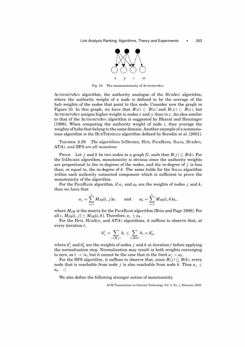
Link Analysis Ranking: Algorithms, Theory and Experiments • 263
Fig. 10. The nonmonotonicity of AUTHORITYAVG.
AUTHORITYAVG algorithm, the authority analogue of the HUBAVG algorithm,where the authority weight of a node is defined to be the average of thehub weights of the nodes that point to this node. Consider now the graph inFigure 10. In this graph, we have that B(x) ⊂ B(z) and B( y) ⊂ B(z), butAUTHORITYAVG assigns higher weight to nodes x and y than to z. An idea similarto that of the AUTHORITYAVG algorithm is suggested by Bharat and Henzinger[1998]. When computing the authority weight of node i, they average theweights of hubs that belong to the same domain. Another example of a nonmono-tone algorithm is the HUBTHESHOLD algorithm defined by Borodin et al. [2001].
THEOREM 4.29. The algorithms INDEGREE, HITS, PAGERANK, SALSA, HUBAVG,AT(k), and BFS are all monotone.
PROOF. Let j and k be two nodes in a graph G, such that B( j ) ⊆ B(k). Forthe INDEGREE algorithm, monotonicity is obvious since the authority weightsare proportional to the in-degrees of the nodes, and the in-degree of j is lessthan, or equal to, the in-degree of k. The same holds for the SALSA algorithmwithin each authority connected component which is sufficient to prove themonotonicity of the algorithm.
For the PAGERANK algorithm, if aj and ak are the weights of nodes j and k,then we have that
aj =n∑
i=1
MPR[i, j ]ai and ak =n∑
i=1
MPR[i, k]ai,
where MPR is the matrix for the PAGERANK algorithm [Brin and Page 1998]. Forall i, MPR[i, j ] ≤ MPR[i, k]. Therefore, aj ≤ ak .
For the HITS, HUBAVG, and AT(k) algorithms, it suffices to observe that, atevery iteration t,
atj =
∑i∈B( j )
hi ≤∑
i∈B(k)
hi = atk ,
where atj and at
k are the weights of nodes j and k at iteration t before applyingthe normalization step. Normalization may result in both weights convergingto zero, as t → ∞, but it cannot be the case that in the limit aj > ak .
For the BFS algorithm, it suffices to observe that, since B( j ) ⊆ B(k), everynode that is reachable from node j is also reachable from node k. Thus aj ≤ak .
We also define the following stronger notion of monotonicity.
ACM Transactions on Internet Technology, Vol. 5, No. 1, February 2005.

264 • A. Borodin et al.
Definition 4.30. An LAR algorithm A is strictly monotone on the class ofgraphs Gn if it has the following property. For every graph G ∈ Gn, and for everypair of nodes j and k in the graph G, B( j ) ⊂ B(k), if and only if A(G)[ j ] <
A(G)[k].
We can now prove the following theorem.
THEOREM 4.31. The algorithms INDEGREE, PAGERANK, SALSA, and BFS arestrictly monotone on the class Gn, while the algorithms HITS, HUBAVG, andMAX are not strictly monotone on the class Gn. The algorithms INDEGREE, HITS,PAGERANK, SALSA, HUBAVG, AT(k), and BFS are all strictly monotone on the classof authority connected graphs GAC
n .
PROOF. The strict monotonicity on the class of the authority connectedgraphs GAC
n follows directly from the proof of Theorem 4.29 for the monotonicityof the algorithms. Similarly, for the strict monotonicity of INDEGREE, PAGERANK,SALSA, and BFS on the class Gn.
For the HITS and HUBAVG algorithms, consider a graph G ∈ Gn consisting oftwo disconnected components. If the components are chosen appropriately, theHITS and HUBAVG algorithms will allocate all the weight to one of the compo-nents, and zero weight to the nodes of the other component. Furthermore, if oneof the two components does not contain a seed node, then the MAX algorithm willallocate zero weight to the nodes of that component. If chosen appropriately, thenodes in the component that receive zero weight violate the strict monotonicityproperty.
A different notion of monotonicity is considered by Chien et al. [2002]. Intheir paper, they study how the weight of a node changes as new links areadded to the node. In this setting, an algorithm is monotone if the weight of anode increases as its in-degree increases.
4.7 Label-Independence
We now introduce the property of label-independence. This property is neededin the axiomatic characterization of the INDEGREE algorithm.
Definition 4.32. Let G ∈ Gn be a graph of size n, and let {1, 2, . . . , n} denotea labeling of the nodes of G. Let A be a LAR algorithm, and let a = A(G)denote the weight vector of A on a graph G ∈ Gn. Let π denote a permutationof the labels of the nodes of G, and let a′ denote the weight vector of A onthe graph with the permuted labels. The algorithm A is label-independent ifa′(π (i)) = a(i).
All the algorithms we considered in this article (INDEGREE, PAGERANK, HITS,SALSA, HUBAVG, AT(k), BAYESIAN, SBAYESIAN BFS) are clearly label-independent.Label-independence is a reasonable property, but one can define reasonable al-gorithms that are not label-independent. For example, an algorithm may chooseto give more weight to a link from a node with a specific label. The algorithm de-fined by Bharat and Henzinger [1998], when computing the authority weight ofa node i, averages the hub weights of the nodes that belong to the same domain.
ACM Transactions on Internet Technology, Vol. 5, No. 1, February 2005.

Link Analysis Ranking: Algorithms, Theory and Experiments • 265
This algorithm is not label-independent since it takes into account the “label”of the node when computing the authority weights.
4.8 An Axiomatic Characterization of the INDEGREE Algorithm
We will now prove that there is a set of properties that characterize the INDEGREE
algorithm.
THEOREM 4.33. An algorithm A that is strictly rank local, monotone, andlabel-independent is rank consistent with the INDEGREE algorithm on the class Gnfor any n ≥ 3. IfA is strictly rank local, strictly monotone, and label-independent,then it is rank equivalent to the INDEGREE algorithm on the class Gn for any n ≥ 3.
PROOF. Let G be a graph of size n ≥ 3, and let a = A(G) be the LAR vector ofalgorithm A on graph G, and w be the LAR vector of INDEGREE. We will modifyG to form graphs G1, and G2, and we use a1, and a2 to denote (respectively) theweight vector of algorithm A on these graphs.
Let i and j be two nodes in G. First, we consider the case that at least oneof i, j has zero in-degree. If wi = wj = 0, that is B(i) = B( j ) = ∅, then fromthe monotonicity of A, we have that ai = aj . Therefore, I (0)
aw(i, j ) = 0, andI (1)aw(i, j ) = 0. If wi > wj = 0, that is, B(i) = ∅, and B( j ) �= ∅, then B(i) ⊂ B( j ).
If A is monotone, ai ≤ aj , thus I (0)aw(i, j ) = 0. If A is strictly monotone, ai < aj ,
thus I (1)aw(i, j ) = 0.
Consider now the case that both i, j have nonzero in-degree. Without loss ofgenerality, assume that wi ≥ wj > 0, or equivalently that node i has at leastas many in-links as node j . The set B(i) ∪ B( j ) of nodes that point to i or j isdecomposed as follows.
—The set C = B(i) ∩ B( j ) contains the nodes that point to both i and j .—The set L = B( j )\C contains the nodes that point to node j , but not to node i.—The set V = B(i) \ C contains the nodes that point to node i, but not to node
j . The set V is further decomposed into the sets R and E. The set R is anarbitrary subset of the set V with cardinality equal to that of L. Since thein-degree of node i is at least as large as that of node j , the set R is welldefined. We also have that, E = V \ R.
Note that some of these sets may be empty, but not all of them can be empty.Specifically, V ∪ C �= ∅, and L ∪ C �= ∅. The set E is empty if and only ifnodes i and j have equal in-degrees. The decomposition of the set B(i) ∪ B( j )is shown in Figure 11(a). The elliptic shapes denote sets of nodes, while thearrows represent the links from a set of nodes to a single node.
Let k �= i, j be an arbitrary node in the graph. We now perform the followingchange to graph G. We remove all links that do not point to i or j , and add linksfrom the nodes in R and C to node k. Let G1 denote the resulting graph. Thegraph G1 is shown in Figure 11(b). Since A is strictly rank local, and the linksto nodes i and j were not affected by the change, we have that
a(i) < a( j ) ⇔ a1(i) < a1( j ). (6)
ACM Transactions on Internet Technology, Vol. 5, No. 1, February 2005.

266 • A. Borodin et al.
Fig. 11. Axiomatic characterization of INDEGREE.
We will now prove that a1(k) = a1( j ). Assume that a1(k) < a1( j ). Let G2denote the graph that we obtain by removing all the links from set R to node i,and adding links from set L to node i. The graph G2 is shown in Figure 11(c).We observe that the graphs G1 and G2 are the same up to a label permutationthat swaps the labels of nodes j and k, and the labels of the nodes in L withthe labels of the nodes in R. Thus, a2( j ) = a1(k), and a2(k) = a1( j ). Therefore,from our assumption that a1(k) < a1( j ), we have a2( j ) < a2(k). However, graphG2 was obtained from graph G1 by performing a local change to node i. Giventhe strict locality assumption, the relative order of the weights of nodes j and kshould remain unaffected, that is, a2( j ) > a2(k), thus reaching a contradiction.We reach the same contradiction if we assume that a1(k) > a1( j ). Therefore, itmust be that a1(k) = a1( j ).
In the graph G1, we have that B(k) ⊆ B(i). We distinguish two cases. IfB(k) = B(i), then the set E is empty. Therefore, wi = wj since i and j havethe same number of in-links. Furthermore, from the monotonicity property(weak or strict) of the algorithm A, we have that a1(i) = a1(k) = a1( j ). FromEquation (6), it follows that a(i) = a( j ).
If B(k) ⊂ B(i), then the set E is not empty, and wi > wj since i has more linksthan j . If A is monotone, then a1(i) ≥ a1(k) = a1( j ). From Equation (6), we havethat a(i) ≥ a( j ). Therefore, for all i, j wi > wj ⇒ ai ≥ aj . Thus, d (0)
r (w, a) = 0,and A and INDEGREE are rank consistent. If A is strictly monotone, then a1(i) >
a1(k) = a1( j ). From Equation (6), we have that a(i) > a( j ). Therefore, for alli, j wi > wj ⇔ ai > aj . Thus, d (1)
r (w, a) = 0, and A and INDEGREE are rankequivalent.
ACM Transactions on Internet Technology, Vol. 5, No. 1, February 2005.

Link Analysis Ranking: Algorithms, Theory and Experiments • 267
The conditions of Theorem 4.33 characterize INDEGREE. All three conditions,label-independence, (strict) monotonicity, and strict rank locality are necessaryfor the proof of the theorem. Assume that we discard the label-independencecondition. Now, define algorithm A that assigns to each link a weight that de-pends on the label of the node from which the link originates. The algorithm setsthe authority weight of each node to be the sum of the link weights that pointto this node. This algorithm is clearly monotone and local, however, if the linkweights are chosen appropriately, it will not be rank consistent with INDEGREE.Assume now that we discard the monotonicity condition. Define an algorithmA, that assigns weight 1 to each node with odd in-degree, and weight 0 toeach node with even in-degree. This algorithm is local and label-independent,but it is clearly not rank consistent with INDEGREE. Monotonicity and label-independence are clearly not sufficient for proving the theorem; we have pro-vided examples of algorithms that are monotone and label-independent, but notrank consistent with the INDEGREE (e.g., the HITS algorithm). Strict monotonic-ity is necessary for proving rank equivalence. The algorithm that assigns equalweight to all nodes is monotone, label-independent, and strictly rank local. Itis rank consistent with INDEGREE, but not rank equivalent.
5. EXPERIMENTAL EVALUATION
In this section, we present an experimental evaluation of the algorithms that weconsider in this article. We study the rankings they produce, and how they relateto each other. The goal of this experimental study is to assess the quality of thealgorithms and, more importantly, to understand how theoretically predictedproperties manifest themselves in a practical setting.
5.1 The Experimental Set-Up
5.1.1 The Queries. We experiment with our algorithms on the following 34different queries.
abortion, affirmative action, alcohol, amusement parks,architecture, armstrong, automobile industries, basketball,blues, cheese, classical guitar, complexity, computationalcomplexity, computational geometry, death penalty,genetic, geometry, globalization, gun control, iraq war,jaguar, jordan, moon landing, movies, national parks, netcensorship, randomized algorithms, recipes, roswell, searchengines, shakespeare, table tennis, weather, vintage cars
Many of these queries have already appeared in previous works [Dwork et al.2001; Lempel and Moran 2000; Kleinberg 1998]. For the remaining queries, weselected queries that correspond to topics for which there are opposing com-munities, such as, “death penalty”, “gun control”, “iraq war”, “globalization”,“moon landing”, or queries that are of interest to different communities, de-pending on the interpretation of the word (for example, “jordan”, “complexity”,“armstrong”). Our objective is to observe how the different algorithms representthese different (usually unrelated, and sometimes opposing) communities in the
ACM Transactions on Internet Technology, Vol. 5, No. 1, February 2005.
268 • A. Borodin et al.
top positions of the ranking. We are also interested in observing the behavior ofthe algorithms when we move from a broad topic (“geometry”, “complexity”) toa more specific subset of this topic (“computational complexity”, “computationalgeometry”). We also selected some queries for which we expect the most rele-vant results not to contain the query words. For example, most search enginesdo not contain the words “search engine”. The same for the query “automobileindustries” which is a variation of the query “automobile manufacturers” thatappears in the work of Kleinberg [1998]. The remaining queries were selectedas interesting queries on broad topics.
The Base Sets for these queries are constructed in the fashion describedby Kleinberg [1998]. We start with a Root Set of pages related to the query.This Root Set is obtained by querying the Google3 search engine. The Root Setconsists of the first 200 pages returned by the search engine. This set is thenexpanded to the Base Set by including nodes that point to, or are pointed to,by the pages in the Root Set. Following the guidelines of Kleinberg [1998], forevery page in the Root Set, we include only the first 50 pages that point tothis page in the order that they are returned by the Google search engine. Wethen extract the links between the pages of the Base Set, and we construct thehyperlink graph.
The next step is to eliminate the navigational links. These are links thatsolely serve the purpose of navigating within a Web site, and they do not conveyan endorsement for the contents of the target page. Finding navigational links isa nontrivial problem that has received some attention in the literature [Davison2000; Bharat and Mihaila 2001]. We adopt the following heuristics for identi-fying navigational links. First, we compare the IP addresses of the two links. Ifthe first three bytes are the same, then we label the link as navigational. If not,we look at the actual URL. This is of the form “http://string1/string2/ · · ·”.The domain identifier is string1. This is of the form “ x1.x2. · · · .xk”. If k ≥ 3,then we use x2. · · · .xk−1 as the domain identifier. If k = 2, we use x1. If the do-main identifiers are the same for the source and target pages of the link, thenthe link is labeled as navigational, and it is discarded. After the navigationallinks are removed, we remove any isolated nodes, and we produce the Base SetP and the graph G = (P, E). Unfortunately, our heuristics do not eliminate allpossible navigational links which in some cases results in introducing clustersof pages from the same domain.
Table I presents statistics for our graphs. The “med out” is the median out-degree, the “avg-out” is the average out-degree, where median and average aretaken over all hub nodes. The “ACC size” is the size of the largest authorityconnected component, that is, the size of the largest connected component inthe authority graph Ga. Recall that the graph Ga is a graph defined on theauthority nodes where there exists an edge between two authorities if theyhave a hub in common.
Matrix Plots: For the purpose of exhibition, we will often present the graph fora query as a matrix plot. A matrix plot, is a bitmap picture of the (transposed)
3http://www.google.com.
ACM Transactions on Internet Technology, Vol. 5, No. 1, February 2005.
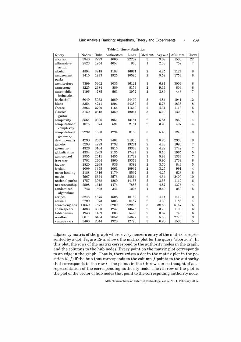
Link Analysis Ranking: Algorithms, Theory and Experiments • 269
Table I. Query Statistics
Query Nodes Hubs Authorities Links Med out Avg out ACC size Usersabortion 3340 2299 1666 22287 3 9.69 1583 22affirmative
action2523 1954 4657 866 1 2.38 752 7
alcohol 4594 3918 1183 16671 2 4.25 1124 8amusementparks
3410 1893 1925 10580 2 5.58 1756 8
architecture 7399 5302 3035 36121 3 6.81 3003 8armstrong 3225 2684 889 8159 2 9.17 806 8automobile
industries1196 785 561 3057 2 3.89 443 7
basketball 6049 5033 1989 24409 3 4.84 1941 12blues 5354 4241 1891 24389 2 5.75 1838 8cheese 3266 2700 1164 11660 2 4.31 1113 5classical
guitar3150 2318 1350 12044 3 5.19 1309 8
complexity 3564 2306 1951 13481 2 5.84 1860 4computational
complexity1075 674 591 2181 2 3.23 497 4
computationalgeometry
2292 1500 1294 8189 3 5.45 1246 3
death penalty 4298 2659 2401 21956 3 8.25 2330 9genetic 5298 4293 1732 19261 2 4.48 1696 7geometry 4326 3164 1815 13363 2 4.22 1742 7globalization 4334 2809 2135 17424 2 8.16 1965 5gun control 2955 2011 1455 11738 3 5.83 1334 7iraq war 3782 2604 1860 15373 3 5.90 1738 8jaguar 2820 2268 936 8392 2 3.70 846 5jordan 4009 3355 1061 10937 2 3.25 991 4moon landing 2188 1316 1179 5597 2 4.25 623 8movies 7967 6624 2573 28814 2 4.34 2409 10national parks 4757 3968 1260 14156 2 3.56 1112 6net censorship 2598 1618 1474 7888 2 4.87 1375 4randomized
algorithms742 502 341 1205 1 2.40 259 5
recipes 5243 4375 1508 18152 2 4.14 1412 10roswell 2790 1973 1303 8487 2 4.30 1186 4search engines 11659 7577 6209 292236 5 38.56 6157 5shakespeare 4383 3660 1247 13575 2 3.70 1199 6table tennis 1948 1489 803 5465 2 3.67 745 6weather 8011 6464 2852 34672 3 5.36 2775 9vintage cars 3460 2044 1920 12796 3 6.26 1580 5
adjacency matrix of the graph where every nonzero entry of the matrix is repre-sented by a dot. Figure 12(a) shows the matrix plot for the query “abortion”. Inthis plot, the rows of the matrix correspond to the authority nodes in the graph,and the columns to the hub nodes. Every point on the matrix plot correspondsto an edge in the graph. That is, there exists a dot in the matrix plot in the po-sition (i, j ) if the hub that corresponds to the column j points to the authoritythat corresponds to the row i. The points in the ith row can be thought of as arepresentation of the corresponding authority node. The ith row of the plot isthe plot of the vector of hub nodes that point to the correspnding authority node.
ACM Transactions on Internet Technology, Vol. 5, No. 1, February 2005.
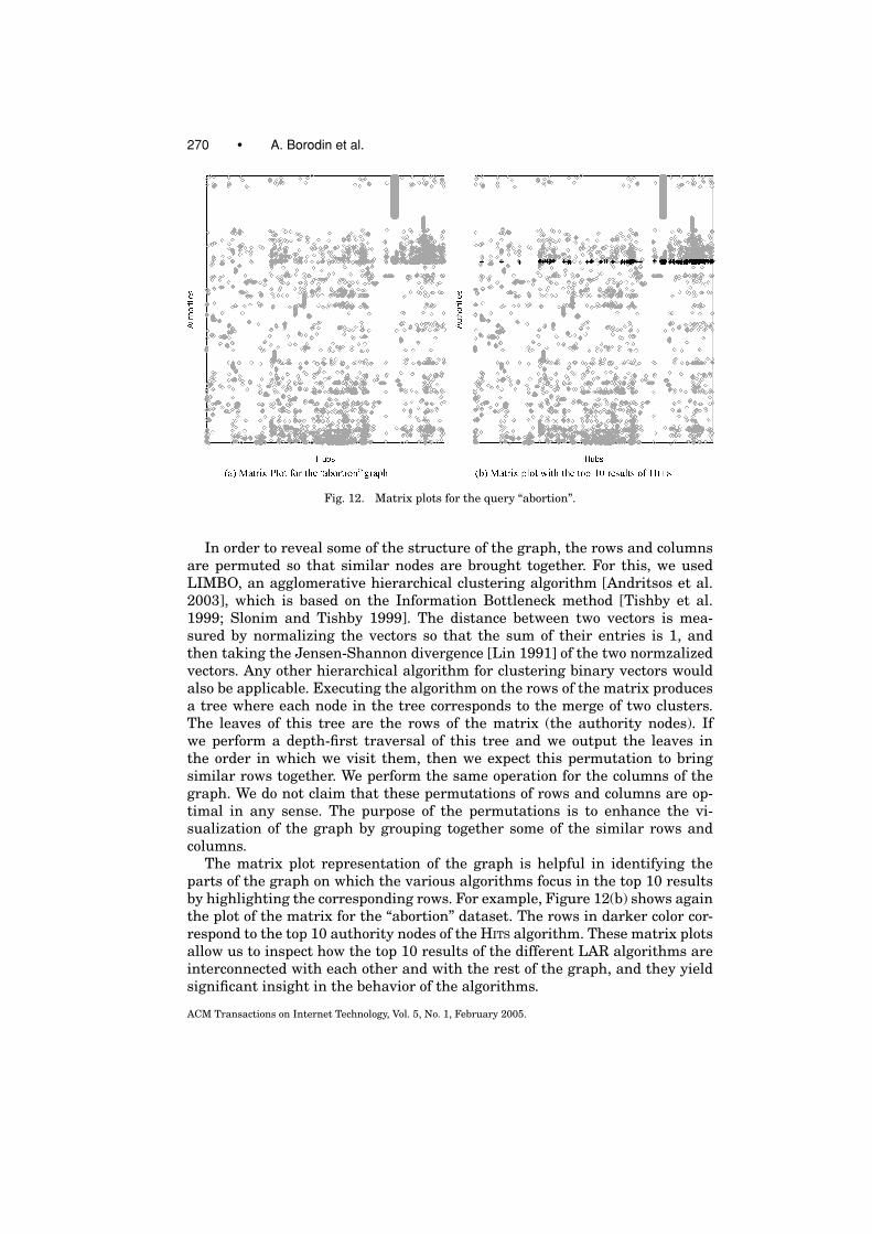
270 • A. Borodin et al.
Fig. 12. Matrix plots for the query “abortion”.
In order to reveal some of the structure of the graph, the rows and columnsare permuted so that similar nodes are brought together. For this, we usedLIMBO, an agglomerative hierarchical clustering algorithm [Andritsos et al.2003], which is based on the Information Bottleneck method [Tishby et al.1999; Slonim and Tishby 1999]. The distance between two vectors is mea-sured by normalizing the vectors so that the sum of their entries is 1, andthen taking the Jensen-Shannon divergence [Lin 1991] of the two normzalizedvectors. Any other hierarchical algorithm for clustering binary vectors wouldalso be applicable. Executing the algorithm on the rows of the matrix producesa tree where each node in the tree corresponds to the merge of two clusters.The leaves of this tree are the rows of the matrix (the authority nodes). Ifwe perform a depth-first traversal of this tree and we output the leaves inthe order in which we visit them, then we expect this permutation to bringsimilar rows together. We perform the same operation for the columns of thegraph. We do not claim that these permutations of rows and columns are op-timal in any sense. The purpose of the permutations is to enhance the vi-sualization of the graph by grouping together some of the similar rows andcolumns.
The matrix plot representation of the graph is helpful in identifying theparts of the graph on which the various algorithms focus in the top 10 resultsby highlighting the corresponding rows. For example, Figure 12(b) shows againthe plot of the matrix for the “abortion” dataset. The rows in darker color cor-respond to the top 10 authority nodes of the HITS algorithm. These matrix plotsallow us to inspect how the top 10 results of the different LAR algorithms areinterconnected with each other and with the rest of the graph, and they yieldsignificant insight in the behavior of the algorithms.
ACM Transactions on Internet Technology, Vol. 5, No. 1, February 2005.

Link Analysis Ranking: Algorithms, Theory and Experiments • 271
5.1.2 Algorithms. We implemented the new algorithms we introduced inSection 3, namely HUBAVG, AT(k), MAX, BFS, BAYESIAN, and SBAYESIAN. For theAT(k) family of algorithms, given a graph G, we compute the distribution ofthe out-degrees in the graph and we experiment with k being the median, andthe average out-degree where median and average are taken over all the hubnodes. We denote these algorithms as AT-MED and AT-AVG, respectively.
We also implemented the HITS, PAGERANK, INDEGREE, and SALSA algorithms.For the PAGERANK algorithm, the jump probability ε usually takes valuesin the interval [0.1, 0.2] [Brin and Page 1998; Ng et al. 2001a]. We observedthat the performance of the PAGERANK algorithm usually improves as we in-crease the value of ε. We set the jump probability ε to be 0.2, a value that issufficiently low and produces satisfactory results.
For all algorithms, we iterate until the L1 difference of the authority weightvectors in two successive iterations becomes less than δ = 10−7, or until 1000iterations have been completed. Although there are more sophisticated methodsfor testing for convergence, we chose this one for the sake of simplicity. In mostcases, the algorithms converge in no more than a hundred iterations.
5.1.3 Measures. The measure that we will use for the evaluation of thequality rankings is precision over top 10. This is the fraction of documents inthe top 10 positions of the ranking that are relevant to the query. Given theimpatient nature of the Web users, we believe that this is an appropriate mea-sure for the evaluation of Web searching and ranking algorithms. Indeed, asearch engine is often judged by the first page of results it returns. We willalso refer to this fraction as the relevance ratio of the algorithm. Similar qual-ity measures are used in the TREC conferences for evaluating Web searchalgorithms.4
We also use a more refined notion of relevance. Given a query, we classify adocument as nonrelevant, relevant, or highly relevant to the topic of the query.High relevance is meant to capture the notion of authoritativeness. A highlyrelevant document is one that should definitely be in the few first page of theresults of a search engine. For example, for the query “movies”, the officialsite for the movie “A Beautiful Mind”5 is relevant to the topic of movies, butit cannot be thought of as highly relevant. However, the Internet Movie DataBase (IMDB) site6 that contains movie information and reviews is a page thatis highly relevant to the topic. This is a result that a Web user would mostlikely want to retrieve when posing the query. The notion of high relevance isalso employed in the TREC conference for topic distillation queries where theobjective is to find the most authoritative pages for a specific topic. For eachalgorithm, we want to estimate the high relevance ratio, the fraction of the top10 results that are highly relevant. Note that every highly relevant page is,of course, relevant so the high relevance ratio is always less or equal to therelevance ratio.
4For TREC data, relevance and high relevance is usually predefined by a set of experts.5http://abeautifulmind.com/.6http://www.imdb.com.
ACM Transactions on Internet Technology, Vol. 5, No. 1, February 2005.

272 • A. Borodin et al.
We are also interested in studying how the algorithms relate to each other.For the comparison of two rankings, we will use the geometric distance mea-sure, d1, defined in Section 4.2.1, and the strict rank distance, d (1)
r , definedin Section 4.2.2. For brevity, we will refer to the strict rank distance as rankdistance, and we will denote it by dr . When computing the d1 distance, thevectors are normalized so that the entries sum to 1. Thus, the maximum d1distance is 2. We will also consider the following two similarity measures forcomparing the top-k results of two algorithms.
—Intersection over top k, I (k): The number of documents that the two rankingshave in common in the top k results.
—Weighted Intersection over top k, W I (k): This is the average intersection overthe top k results, where the average is taken over the intersection over thetop 1, top 2, up to top k. The weighted intersection is given by the followingformula.
W I (k) = 1k
k∑i=1
I (i).
In our study, we measure the similarity over the top 10 results.
5.1.4 User Study. In order to assess the relevance of the documents, weperformed a user study. The study was performed online.7 The introductorypage contained the queries with links to the results, together with some instruc-tions. By clicking on a query, the union of the top 10 results of all algorithmswas presented to the user. The results were permuted so that they appearedin a random order and no information was revealed about the algorithm(s)that introduced each result in the collection. The users were then asked to rateeach document as “Highly Relevant”, “Relevant”, or “NonRelevant”. They wereinstructed to mark a page as “Highly Relevant” if they would definitely liketo see if within the top positions of a search engine. An option “Don’t Know”(chosen as default) was also given in the case that the user could not assessthe relevance of the result. When pressing the submit button, their feedbackwas stored into a file. No information was recorded about the users, respect-ing their anonymity. No queries were assigned to any users, they were free todo whichever ones, and however many they wanted. On average seven usersrated each query. The maximum was twenty two, for the query “abortion”, andthe minimum three, for the query “computational geometry”. The number ofusers per query are shown in Table I. The study was conducted mostly amongfriends and fellow grad students. Although they are not all experts on all of thetopics, we believe that their feedback gives a useful indication about the actualrelevance of the documents.8
We utilize the user’s feedback in the following way. Given the users’ feedbackfor a specific document, we rate the document as “Relevant” if the “Relevant”and “Highly Relevant” votes are more than the “Non-Relevant” votes (ties areresolved in favor of “Non-Relevant”). Among the documents that are deemed as
7The URL for the study is http://www.cs.toronto.edu/∼tsap/cgi-bin/entry.cgi.8The results of the study may be slightly biased towards the opinion of people of Greek origin.
ACM Transactions on Internet Technology, Vol. 5, No. 1, February 2005.

Link Analysis Ranking: Algorithms, Theory and Experiments • 273
“Relevant”, we rate as “Highly Relevant” the ones for which the “Highly Rele-vant” votes are more than the “Relevant” ones. We can now compute the rele-vance ratios for the algorithms by using the relevance ratings of the documents.
5.2 Evaluation of the LAR Algorithms
In this section, we study the aggregate behavior of the algorithms. The resultsfor all queries are posted on the Web9 in a format that is easy to understandand navigate. We strongly encourage the reader to browse through the resultswhile reading this part of the article. Appendix A contains tables with the top 10results for three sample queries (“abortion”, “amusement parks”, “classical gui-tar”) that are referenced often in the next sections. In these Tables, the resultsthat are labeled highly relevant appear in boldface, the relevant ones appear initalics, and the nonrelevant appear in regular font. Due to space constraints, weomit the results of the SALSA and SBAYESIAN algorithms. In almost all queries,they are identical to those of INDEGREE. Tables II, III report the quality ratiosof each algorithm for each query. In each row, the highlighted value is the bestratio for this query. For each algorithm, we also compute the average, the stan-dard deviation, the minimum, and the maximum values for all quality ratios.Recall, that for the relevance ratio, we consider documents that are markedeither “Relevant” or “Highly Relevant”, so the relevance ratio is always greateror equal to the high relevance ratio. For the purpose of comparing algorithms,we also report the average values of all our similarity and distance measuresin Appendix A.
The qualitative evaluation reveals that all algorithms fall, to some extent,victim to topic drift. That is, they promote pages that are not related to thetopic of the query. In terms of average high relevance, more than half (and asmany as 8 out of 10 for the case of HITS) of the results in the top 10 are nothighly relevant. This is significant for the quality of the algorithms since thehighly relevant documents represent the ones that the users would actuallywant to see in the top positions of the ranking, as opposed to the ones that theyfound just relevant to the topic. The performance improves when we considerrelevance instead of high relevance. Still, the average relevance ratio is nevermore than 78%, that is, even for the best algorithm, on average 2 out of thetop 10 documents are irrelevant to the query. Furthermore, there exist queriessuch as “armstrong” and “jaguar” for which no algorithm was able to producesatisfactory results.
The algorithm that emerges as the “best” is the BFS algorithm. It exhibitsthe best high relevance and relevance ratio on average, and it is the algorithmthat most often achieves the maximum relevance ratio (for the high relevanceratio the record is held by the MAX algorithm). Furthermore, as the low standarddeviation indicates, and the study of the results reveals, it exhibits a robust andconsistent behavior across queries.
At the other end of the spectrum, the HITS and the PAGERANK algorithmsemerge as the “worst” algorithms, exhibiting the lowest ratios, with HITS be-ing slightly worse. However, although they have similar (poor) performance on
9http://www.cs.toronto.edu/∼tsap/experiments/journal/.
ACM Transactions on Internet Technology, Vol. 5, No. 1, February 2005.

274 • A. Borodin et al.
Table II. High Relevance Ratio
Query HITS PAGERANK INDEGREE SALSA HUBAVG MAX AT-MED AT-AVG BFS BAYESIAN SBAYESIAN
abortion 30% 10% 40% 40% 30% 40% 30% 30% 30% 30% 40%affirmative
action30% 0% 40% 40% 0% 0% 0% 0% 60% 30% 40%
alcohol 60% 30% 60% 60% 60% 50% 50% 50% 70% 50% 60%amusement
parks50% 10% 30% 40% 0% 70% 10% 0% 40% 90% 30%
architecture 0% 30% 70% 70% 0% 60% 60% 0% 50% 0% 70%armstrong 0% 0% 0% 0% 0% 0% 0% 0% 0% 0% 0%automobile
industries0% 10% 10% 20% 0% 0% 0% 0% 40% 0% 10%
basketball 0% 60% 20% 20% 0% 10% 10% 10% 60% 10% 20%blues 60% 40% 40% 40% 50% 50% 50% 50% 20% 40% 40%cheese 0% 0% 0% 0% 0% 0% 0% 0% 10% 0% 0%classical
guitar40% 30% 30% 30% 0% 40% 0% 0% 40% 30% 30%
complexity 0% 30% 20% 20% 0% 70% 50% 0% 50% 0% 20%computational
complexity30% 30% 30% 30% 40% 30% 30% 30% 20% 30% 30%
computationalgeometry
40% 20% 40% 40% 40% 40% 50% 40% 40% 30% 40%
death penalty 70% 30% 70% 70% 50% 80% 80% 80% 80% 80% 60%genetic 80% 20% 70% 70% 60% 70% 70% 70% 60% 80% 70%geometry 60% 10% 50% 50% 40% 70% 70% 60% 60% 60% 50%globalization 0% 30% 20% 20% 0% 0% 0% 0% 30% 0% 20%gun control 0% 50% 70% 70% 60% 60% 60% 60% 60% 50% 70%iraq war 0% 10% 10% 10% 0% 10% 0% 0% 40% 10% 10%jaguar 0% 20% 0% 0% 0% 0% 0% 0% 10% 0% 0%jordan 0% 10% 20% 20% 20% 40% 40% 40% 30% 20% 20%moon landing 0% 20% 10% 10% 0% 0% 0% 0% 80% 0% 10%movies 10% 10% 30% 30% 40% 70% 70% 70% 40% 50% 30%national parks 0% 50% 10% 10% 60% 60% 60% 0% 50% 0% 10%net censorship 0% 20% 80% 80% 60% 80% 80% 80% 80% 70% 80%randomized
algorithms0% 40% 10% 10% 0% 0% 0% 0% 10% 10% 10%
recipes 0% 10% 60% 60% 10% 60% 60% 70% 50% 50% 60%roswell 0% 0% 0% 0% 0% 10% 10% 0% 10% 0% 0%search engines 60% 70% 100% 100% 100% 100% 100% 100% 90% 50% 100%shakespeare 0% 20% 50% 50% 50% 70% 70% 70% 60% 50% 50%table tennis 50% 20% 50% 50% 50% 50% 50% 50% 40% 40% 50%weather 60% 20% 60% 60% 30% 60% 50% 50% 70% 60% 60%vintage cars 0% 0% 40% 40% 0% 40% 40% 0% 30% 10% 40%
avg 21% 22% 36% 37% 25% 41% 37% 30% 44% 30% 36%max 80% 70% 100% 100% 100% 100% 100% 100% 90% 90% 100%min 0% 0% 0% 0% 0% 0% 0% 0% 0% 0% 0%stdev 27% 17% 26% 26% 28% 30% 31% 32% 23% 28% 26%
average, the two algorithms exhibit completely different behaviors. The behav-ior of the HITS algorithm is erratic. As the standard deviation indicates and thequery results reveal, the performance of HITS exhibits large variance. There arequeries (such as “amusement parks”, “genetic”, “classical guitar”, “table tennis”)for which the HITS algorithm exhibits good relevance and high relevance ratiosbut, at the same time, there are many queries (such as, “basketball”, “gun con-trol”, “moon landing”,“recipes”) for which HITS has a 0% relevance ratio. Thisis related to the Tightly Knit Community(TKC) effect. HITS is known to favornodes that belong to the most tightly interconnected component in the graph.
ACM Transactions on Internet Technology, Vol. 5, No. 1, February 2005.
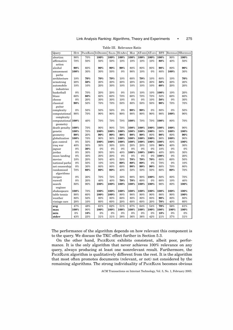
Link Analysis Ranking: Algorithms, Theory and Experiments • 275
Table III. Relevance Ratio
Query HITS PAGERANK INDEGREE SALSA HUBAVG MAX AT-MED AT-AVG BFS BAYESIAN SBAYESIAN
abortion 90% 70% 100% 100% 100% 100% 100% 100% 100% 90% 100%affirmative
action70% 50% 50% 50% 10% 10% 10% 10% 80% 40% 50%
alcohol 90% 60% 90% 90% 90% 80% 80% 80% 90% 80% 90%amusement
parks100% 30% 30% 50% 0% 90% 10% 0% 80% 100% 30%
architecture 10% 70% 70% 70% 10% 60% 70% 10% 60% 10% 70%armstrong 20% 50% 20% 20% 20% 20% 20% 20% 50% 20% 20%automobile
industries10% 10% 20% 30% 10% 10% 10% 10% 60% 20% 20%
basketball 0% 70% 20% 20% 0% 10% 10% 10% 100% 10% 20%blues 60% 80% 60% 60% 70% 60% 70% 70% 50% 60% 60%cheese 0% 20% 30% 30% 10% 0% 0% 10% 50% 0% 30%classical
guitar90% 50% 70% 70% 50% 80% 50% 50% 90% 70% 70%
complexity 0% 50% 50% 50% 0% 90% 90% 0% 80% 0% 50%computational
complexity90% 70% 90% 90% 90% 90% 90% 90% 90% 100% 90%
computationalgeometry
100% 40% 70% 70% 70% 100% 70% 70% 100% 80% 70%
death penalty 100% 70% 90% 90% 70% 100% 100% 100% 100% 100% 90%genetic 100% 70% 100% 100% 100% 100% 100% 100% 90% 100% 100%geometry 90% 20% 90% 90% 90% 90% 90% 80% 90% 80% 90%globalization 100% 70% 90% 90% 100% 100% 100% 100% 90% 100% 90%gun control 0% 50% 100% 100% 100% 100% 100% 100% 100% 80% 100%iraq war 40% 30% 30% 30% 10% 20% 20% 10% 90% 40% 30%jaguar 0% 30% 0% 0% 0% 0% 0% 0% 10% 0% 0%jordan 0% 30% 30% 30% 40% 100% 100% 100% 40% 30% 30%moon landing 0% 30% 20% 20% 0% 0% 0% 0% 100% 0% 20%movies 10% 20% 50% 40% 50% 70% 70% 70% 60% 60% 50%national parks 0% 50% 10% 10% 80% 80% 80% 0% 70% 0% 10%net censorship 0% 30% 80% 80% 60% 90% 90% 90% 80% 70% 80%randomized
algorithms70% 80% 80% 80% 40% 50% 50% 50% 60% 80% 70%
recipes 0% 20% 70% 70% 30% 90% 90% 100% 80% 80% 70%roswell 0% 20% 40% 40% 70% 70% 60% 0% 60% 10% 40%search
engines80% 90% 100% 100% 100% 100% 100% 100% 90% 80% 100%
shakespeare 100% 70% 100% 100% 100% 100% 100% 100% 100% 100% 100%table tennis 90% 60% 100% 100% 90% 90% 90% 90% 90% 90% 100%weather 80% 50% 80% 80% 60% 80% 80% 80% 90% 80% 80%vintage cars 20% 10% 60% 60% 20% 60% 60% 20% 70% 40% 60%
avg 47% 48% 61% 62% 51% 67% 64% 54% 78% 56% 61%max 100% 90% 100% 100% 100% 100% 100% 100% 100% 100% 100%min 0% 10% 0% 0% 0% 0% 0% 0% 10% 0% 0%stdev 43% 23% 31% 31% 38% 36% 36% 42% 21% 37% 31%
The performance of the algorithm depends on how relevant this component isto the query. We discuss the TKC effect further in Section 5.3.
On the other hand, PAGERANK exhibits consistent, albeit poor, perfor-mance. It is the only algorithm that never achieves 100% relevance on anyquery, always producing at least one nonrelevant result. Furthermore, thePAGERANK algorithm is qualitatively different from the rest. It is the algorithmthat most often promotes documents (relevant, or not) not considered by theremaining algorithms. The strong individuality of PAGERANK becomes obvious
ACM Transactions on Internet Technology, Vol. 5, No. 1, February 2005.

276 • A. Borodin et al.
when examining the average distance of PAGERANK to the remaining algorithms(Tables IV, V, VI, VII in Appendix A), especially for the I and W I measures.This is something to be expected since the philosophy of the algorithm is differ-ent. Furthermore, the Base Set for each query is constructed in a way that ismeant to take advantage of the mutual reinforcing relation between hubs andauthorities, a property that does not affect the PAGERANK algorithm. We discussthis more in Section 5.3.
The MAX algorithm emerges as the second best option after BFS, and it ac-tually achieves the best high relevance score. The quality of the MAX algorithmusually depends on the quality of the seed node and the nodes with the highestin-degree. We actually observed that, in most cases, the top 10 nodes returnedby MAX are a subset of the ten nodes with the highest in-degree, and the tennodes that are most co-cited with the seed node. The ratios of MAX indicate thatthe seed node is usually relevant to the query.
This observation agrees with the relatively high quality of the results of theINDEGREE algorithm. On average, 3 out of 10 of the most popular documents arehighly relevant, and 6 out 10 are relevant. Because of its simplicity, one wouldexpect the quality of the INDEGREE algorithm to set the bar for the remainingalgorithms. Surprisingly, in many queries, the INDEGREE algorithm outperformssome of the more sophisticated algorithms. We should note though that, due tothe simplicity of the algorithm, the INDEGREE algorithm is the one that is mostaffected by the choice of the search engine that is used for generating the BaseSet of Web pages. Therefore, the performance of the INDEGREE algorithm reflects,in part, the quality of the Google search engine which uses, to some extent, linkanalysis techniques. It would be most interesting if one could generate a BaseSet using a search engine that does not make use of any link analysis.
In our experiments, in most queries, the SALSA algorithm produces the sametop 10 pages as the INDEGREE algorithm. The similarity of the two algorithmsbecomes obvious in the average values of all similarity measures in the tables ofAppendix A, and especially in the I and W I measures. As can be seen in Table I,the graphs in our experiments contain a giant authority connected componentwhich attracts most of the authority weight of the SALSA algorithm. As a result,the algorithm reduces to the INDEGREE algorithm.
For the other variants of HITS, the HUBAVG is the one that performs the worst,only slightly better than HITS. HUBAVG suffers from its own TKC effect that wedescribe in Section 5.3. For the AT-MED and AT-AVG, close examination of theresults reveals that they usually have the same ratios as either the HITS or theMAX algorithm. In most cases, the top 10 results of these algorithms are a subsetof the union of the top 10 results of HITS and MAX. Thus, it is not surprisingthat the average performance ratios of AT-MED and AT-AVG take values betweenthe ratios of MAX and HITS. We also note that all derivatives of HITS (includingMAX) exhibit similar erratic behavior to that of HITS. This is due to the variousTKC phenomena that we describe in the next section.
The study of the performance of the Bayesian algorithms provides the mostintriguing observation of the experimental evaluation. The performance of theSBAYESIAN algorithm is almost identical to that of the INDEGREE algorithm.This is corroborated by the average similarity measures in Appendix A. For
ACM Transactions on Internet Technology, Vol. 5, No. 1, February 2005.
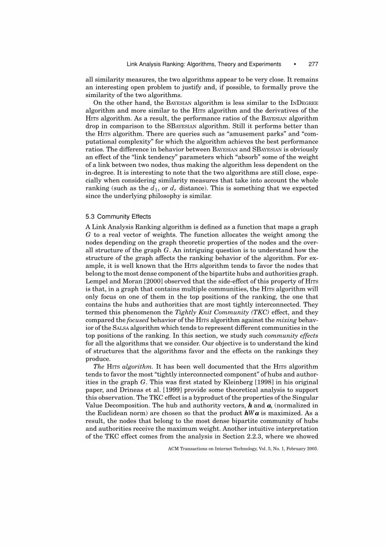
Link Analysis Ranking: Algorithms, Theory and Experiments • 277
all similarity measures, the two algorithms appear to be very close. It remainsan interesting open problem to justify and, if possible, to formally prove thesimilarity of the two algorithms.
On the other hand, the BAYESIAN algorithm is less similar to the INDEGREE
algorithm and more similar to the HITS algorithm and the derivatives of theHITS algorithm. As a result, the performance ratios of the BAYESIAN algorithmdrop in comparison to the SBAYESIAN algorithm. Still it performs better thanthe HITS algorithm. There are queries such as “amusement parks” and “com-putational complexity” for which the algorithm achieves the best performanceratios. The difference in behavior between BAYESIAN and SBAYESIAN is obviouslyan effect of the “link tendency” parameters which “absorb” some of the weightof a link between two nodes, thus making the algorithm less dependent on thein-degree. It is interesting to note that the two algorithms are still close, espe-cially when considering similarity measures that take into account the wholeranking (such as the d1, or dr distance). This is something that we expectedsince the underlying philosophy is similar.
5.3 Community Effects
A Link Analysis Ranking algorithm is defined as a function that maps a graphG to a real vector of weights. The function allocates the weight among thenodes depending on the graph theoretic properties of the nodes and the over-all structure of the graph G. An intriguing question is to understand how thestructure of the graph affects the ranking behavior of the algorithm. For ex-ample, it is well known that the HITS algorithm tends to favor the nodes thatbelong to the most dense component of the bipartite hubs and authorities graph.Lempel and Moran [2000] observed that the side-effect of this property of HITS
is that, in a graph that contains multiple communities, the HITS algorithm willonly focus on one of them in the top positions of the ranking, the one thatcontains the hubs and authorities that are most tightly interconnected. Theytermed this phenomenon the Tightly Knit Community (TKC) effect, and theycompared the focused behavior of the HITS algorithm against the mixing behav-ior of the SALSA algorithm which tends to represent different communities in thetop positions of the ranking. In this section, we study such community effectsfor all the algorithms that we consider. Our objective is to understand the kindof structures that the algorithms favor and the effects on the rankings theyproduce.
The HITS algorithm. It has been well documented that the HITS algorithmtends to favor the most “tightly interconnected component” of hubs and author-ities in the graph G. This was first stated by Kleinberg [1998] in his originalpaper, and Drineas et al. [1999] provide some theoretical analysis to supportthis observation. The TKC effect is a byproduct of the properties of the SingularValue Decomposition. The hub and authority vectors, h and a, (normalized inthe Euclidean norm) are chosen so that the product hWa is maximized. As aresult, the nodes that belong to the most dense bipartite community of hubsand authorities receive the maximum weight. Another intuitive interpretationof the TKC effect comes from the analysis in Section 2.2.3, where we showed
ACM Transactions on Internet Technology, Vol. 5, No. 1, February 2005.

278 • A. Borodin et al.
Fig. 13. The TKC effect for the HITS algorithm for the query “gun control”.
that the weight on node i, after n iterations, is proportional to the number of(BF)n paths that leave node i.
The TKC effect is prominent in our experiments with the HITS algorithm,most of the time leading to a severe topic drift. Consider, for example, the query“gun control”. Figure 13 shows the matrix plot of the graph and the top 10 resultsfor HITS. In this query, HITS gets trapped in a tightly interconnected componentof 69 nodes (63 hubs and 37 authorities) which is completely disconnected fromthe rest of the graph, and obviously unrelated to the query. Similar phenomenaappear in many of the queries that we have tested (examples include, “vintagecars”, “recipes”, “movies”, “complexity”).
Consider now the query “abortion”. Figure 14(a) shows the plot of the graphfor this query. The graph contains two separated, but not completely discon-nected, communities of Web pages: the pro-choice community, and the pro-lifecommunity. The pro-life community contains a set X of 37 hubs from a religiousgroup10 which form a complete bipartite graph with a set Y of 288 authoritynodes. These appear as a vertical strip in the top-right part of the plot. Thistightly interconnected set of nodes attracts the HITS algorithm to that commu-nity, and it ranks these 37 nodes as the best hubs. Among the 288 authori-ties, HITS ranks in the top 10, the authorities that are better interconnectedwith the remaining hubs in the community. The plot for the top 10 results forHITS is shown in Figure 14(b). The points in darker color correspond to thetop 10 results of the HITS algorithm. The results can be found in Table VIII inAppendix A.
10http://www.abortion-and-bible.com/.
ACM Transactions on Internet Technology, Vol. 5, No. 1, February 2005.

Link Analysis Ranking: Algorithms, Theory and Experiments • 279
Fig. 14. The query “abortion”.
The HUBAVG Algorithm. In Section 3.1, we showed that the HUBAVG algo-rithm computes the Singular Value Decomposition of the normalized matrixWe. Therefore, we expect the HUBAVG algorithm to exhibit similar TKC effectsin the normalized authority space defined by the matrix We. This is indeedthe case, and it accounts for the poor behavior of the HUBAVG algorithm. How-ever, the normalization causes the HUBAVG algorithm to differ significantly fromHITS. The HUBAVG algorithm favors tightly-knit communities, but it also posesthe additional requirement of exclusiveness. That is, it requires that the hubsare exclusive to the community to which they belong. As a result, the HUBAVG
algorithm tends to favor tightly-knit, isolated components in the graph that con-tain nodes of high in-degree. These correspond to long, thin horizontal strips inour plots. If such a strip exists, that is, if there exists a large set of hubs that all
ACM Transactions on Internet Technology, Vol. 5, No. 1, February 2005.

280 • A. Borodin et al.
Fig. 15. HITS and HUBAVG for the query “recipes”.
point to just a few authorities in the graph, then this community receives mostof the weight of the HUBAVG algorithm. Unfortunately, this occurs often in ourexperiments, resulting in topic drift for HUBAVG.
Figure 15 shows the plot of the graph for the query “recipes”. The communi-ties that attract the top 10 results of HITS and HUBAVG are marked on the plot.The tables contain the top 10 tuples for each algorithm. The community on newsand advertising that attracts HITS contains a set of hubs that point to nodes
ACM Transactions on Internet Technology, Vol. 5, No. 1, February 2005.

Link Analysis Ranking: Algorithms, Theory and Experiments • 281
outside the community. This corresponds to the vertical strip above the markedrows for HITS. HUBAVG escapes this community, but it assigns almost all weightto a community of just three nodes that are interconnected by 45 hubs. Onlytwo out of these 45 hubs point to nodes other than these three nodes. Note that,in order for such a structure to attract HUBAVG, the authorities (or at least someof the authorities) must have sufficiently large in-degree. In this case, the topthree nodes for for HUBAVG correspond to the nodes with the 10th, 11th and 13thhighest in-degree in the graph. This is a typical example of the behavior of theHUBAVG algorithm. Although the HUBAVG algorithm manages to escape the com-munities that pull HITS into topic drift, it still falls victim to its own TKC effect.
Consider the HUBAVG algorithm on the query “abortion”. The authority nodesin the set Y are not all of equal strength. Some of them are well interconnectedwith other hubs in the pro-life community (the ones ranked high by HITS), butthe large majority of them are pointed to only by the hubs in the set X . Recallthat the HUBAVG algorithm requires that the hubs point only (or at least mainly)to good authorities. Most of the authorities in Y are poor. As a result, the hubsin X are penalized. The HUBAVG algorithm avoids the pro-life community andfocuses on the pro-choice one. Note that this is the community that contains thenode with the maximum in-degree. The top 10 results of HUBAVG are plotted inFigure 14(c).
The MAX algorithm. The influence of the various communities on the rank-ing of the MAX algorithm is primarily exerted through the seed node. Thecommunity that contains the seed node and the co-citation of the seed nodewith the remaining nodes in the community determine the focus of the MAX al-gorithm. For example, in the “movies” query, the seed node is the Internet MovieDatabase11 (IMDB), and the algorithm converges to a set of movie databasesand movie reviews sites. Similarly for the “net censorship” query, where theseed node is the Electronic Frontier Foundation12 (EFF), the algorithm outputshighly relevant results. In both these cases, the MAX algorithm manages bestto distill the relevant pages from the community to which it converges. On theother hand, in the case of the “affirmative action” query, the seed node is acopyright page from the University of Pennsylvania and, as a result, the MAX
algorithm outputs a community of university home pages.There are cases where the seed node may belong to more than one commu-
nity. For example, for the query “basketball”, the seed node is the NBA officialWeb page.13 This page belongs to the basketball community, but it has thehighest overlap with a community of nodes from MSN,14 which causes the MAX
algorithm to converge to this community. It may also be the case that thereare multiple seed nodes in the graph. For example, for the “randomized algo-rithms” query, there are two seeds in the graph, one on algorithms, and oneon computational geometry. As a result, the algorithm mixes pages of bothcommunities.
11http://www.imdb.com.12http://www.eff.org.13http://www.nba.com.14http://www.msn.com.
ACM Transactions on Internet Technology, Vol. 5, No. 1, February 2005.
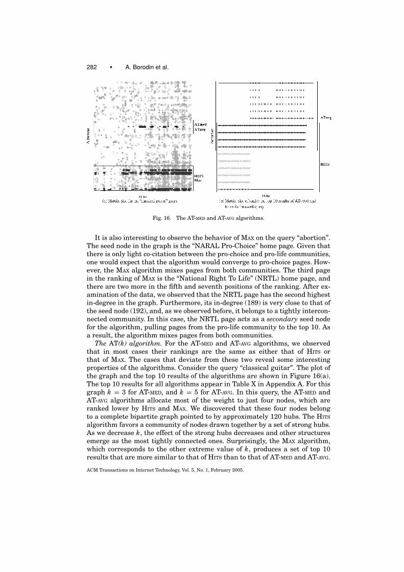
282 • A. Borodin et al.
Fig. 16. The AT-MED and AT-AVG algorithms.
It is also interesting to observe the behavior of MAX on the query “abortion”.The seed node in the graph is the “NARAL Pro-Choice” home page. Given thatthere is only light co-citation between the pro-choice and pro-life communities,one would expect that the algorithm would converge to pro-choice pages. How-ever, the MAX algorithm mixes pages from both communities. The third pagein the ranking of MAX is the “National Right To Life” (NRTL) home page, andthere are two more in the fifth and seventh positions of the ranking. After ex-amination of the data, we observed that the NRTL page has the second highestin-degree in the graph. Furthermore, its in-degree (189) is very close to that ofthe seed node (192), and, as we observed before, it belongs to a tightly intercon-nected community. In this case, the NRTL page acts as a secondary seed nodefor the algorithm, pulling pages from the pro-life community to the top 10. Asa result, the algorithm mixes pages from both communities.
The AT(k) algorithm. For the AT-MED and AT-AVG algorithms, we observedthat in most cases their rankings are the same as either that of HITS orthat of MAX. The cases that deviate from these two reveal some interestingproperties of the algorithms. Consider the query “classical guitar”. The plot ofthe graph and the top 10 results of the algorithms are shown in Figure 16(a).The top 10 results for all algorithms appear in Table X in Appendix A. For thisgraph k = 3 for AT-MED, and k = 5 for AT-AVG. In this query, the AT-MED andAT-AVG algorithms allocate most of the weight to just four nodes, which areranked lower by HITS and MAX. We discovered that these four nodes belongto a complete bipartite graph pointed to by approximately 120 hubs. The HITS
algorithm favors a community of nodes drawn together by a set of strong hubs.As we decrease k, the effect of the strong hubs decreases and other structuresemerge as the most tightly connected ones. Surprisingly, the MAX algorithm,which corresponds to the other extreme value of k, produces a set of top 10results that are more similar to that of HITS than to that of AT-MED and AT-AVG.
ACM Transactions on Internet Technology, Vol. 5, No. 1, February 2005.

Link Analysis Ranking: Algorithms, Theory and Experiments • 283
We observed the similar phenomena for the queries “cheese” and “amusementparks”.
In order to better understand the mechanics of the threshold algorithms, weconsider the “roswell” query. In this case, the AT-AVG produces the same top 4authorities as HITS, but the lower part of the ranking is completely different.In this graph, k = 4 for the AT-AVG algorithm. Figure 16(b) shows the plot forthe top 10 authorities of both algorithms. The middle part corresponds to thecommon authorities, the bottom rows are the authorities of HITS, and the upperrows are the authorities of AT-AVG. Note that the authorities of HITS are moretightly interconnected. However, given that k = 4, all hubs receive the sameweight, since they all point to the middle authorities which are the strongest.These four authorities play a role similar to that of the seed in the MAX
algorithm. Therefore, the authorities of AT-AVG are ranked higher because theyhave higher co-citation with the “seed” nodes despite the fact that they are notas well interconnected. It seems that as we decrease the value of k, the effectof the in-degree increases.
The INDEGREE and SALSA algorithms. The effect of different communities tothe INDEGREE algorithm is straightforward. Communities that contain nodeswith high in-degree will be promoted, while communities that do not contain“popular” nodes are not represented regardless of how tightly interconnectedthey are. As a result, INDEGREE usually mixes the results of various communitiesin the top 10 results. One characteristic example is the “genetic” query wherethe INDEGREE algorithm is the only one to introduce a page from the GeneticAlgorithms community. The simplistic approach of the INDEGREE algorithm ap-pears to work relatively well in practice. However, it has no defense mechanismagainst spurious authorities, that is, nodes with high in-degree that are not re-lated to the query, as in the case of the “amusement parks” query. Another suchexample is the “basketball” query, where the algorithm is drawn to the set ofspurious authorities from the MSN community.
As we have already discussed, in most cases, the SALSA algorithm outputsthe same top 10 results as INDEGREE. The “amusement parks” query is oneof the rare cases where the rankings of the two algorithms differ. For this query,the node with the highest in-degree is a completely isolated node. SALSA is de-signed to handle such situations (i.e., nodes that are very popular, but belong toweak communities), so the high in-degree isolated node does not appear in thetop 10 of the SALSA algorithm. The top 10 results for both SALSA and INDEGREE
algorithms are shown in Figure 17. The premise of SALSA is interesting. It setsthe weight of a node as a combination of the popularity of the community it be-longs to as well as its popularity within the community. However, a community,in this case, is defined as an authority connected component (ACC) of the graph.This is a very strong definition since, if a node shares even just one hub with theACC, it immediately becomes part of the community. It would be interestingto experiment with SALSA on graphs that contain multiple ACCs of comparablesize, and observe how the algorithm mixes between the different communities.In our experiments, all graphs contain a giant ACC and many small ACCs thatdo not contribute to the ranking. Thus, the SALSA algorithm reduces to INDEGREE
with the additional benefit of avoiding the occasional isolated high in-degree
ACM Transactions on Internet Technology, Vol. 5, No. 1, February 2005.

284 • A. Borodin et al.
Fig. 17. The query “amusement parks”.
node for the queries “amusement parks”, “automobile industries”, “moon land-ing”, “movies”, and “national parks”.
The “amusement parks” query is particularly interesting since it revealsthe behavior of the algorithms in extreme settings. The top 10 results for allalgorithms appear in Table IX in Appendix A. The plot of the graph for thisquery is shown in Figure 17. Both MAX and HUBAVG allocate all their weightto the isolated node with the maximum in-degree, and zero to the rest of thenodes. The HITS algorithm escapes this component easily, and converges to themost relevant community. The AT-MED, AT-AVG algorithms converge again to asmall tight bipartite graph different from that of HITS.
ACM Transactions on Internet Technology, Vol. 5, No. 1, February 2005.
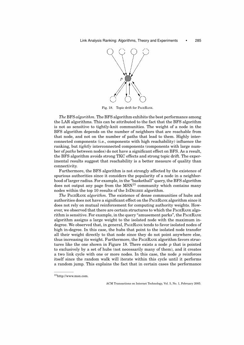
Link Analysis Ranking: Algorithms, Theory and Experiments • 285
Fig. 18. Topic drift for PAGERANK.
The BFS algorithm. The BFS algorithm exhibits the best performance amongthe LAR algorithms. This can be attributed to the fact that the BFS algorithmis not as sensitive to tightly-knit communities. The weight of a node in theBFS algorithm depends on the number of neighbors that are reachable fromthat node, and not on the number of paths that lead to them. Highly inter-connected components (i.e., components with high reachability) influence theranking, but tightly interconnected components (components with large num-ber of paths between nodes) do not have a significant effect on BFS. As a result,the BFS algorithm avoids strong TKC effects and strong topic drift. The exper-imental results suggest that reachability is a better measure of quality thanconnectivity.
Furthermore, the BFS algorithm is not strongly affected by the existence ofspurious authorities since it considers the popularity of a node in a neighbor-hood of larger radius. For example, in the “basketball” query, the BFS algorithmdoes not output any page from the MSN15 community which contains manynodes within the top 10 results of the INDEGREE algorithm.
The PAGERANK algorithm. The existence of dense communities of hubs andauthorities does not have a significant effect on the PAGERANK algorithm since itdoes not rely on mutual reinforcement for computing authority weights. How-ever, we observed that there are certain structures to which the PAGERANK algo-rithm is sensitive. For example, in the query “amusement parks”, the PAGERANK
algorithm assigns a large weight to the isolated node with the maximum in-degree. We observed that, in general, PAGERANK tends to favor isolated nodes ofhigh in-degree. In this case, the hubs that point to the isolated node transferall their weight directly to that node since they do not point anywhere else,thus increasing its weight. Furthermore, the PAGERANK algorithm favors struc-tures like the one shown in Figure 18. There exists a node p that is pointedto exclusively by a set of hubs (not necessarily many of them), and it createsa two link cycle with one or more nodes. In this case, the node p reinforcesitself since the random walk will iterate within this cycle until it performsa random jump. This explains the fact that in certain cases the performance
15http://www.msn.com.
ACM Transactions on Internet Technology, Vol. 5, No. 1, February 2005.
286 • A. Borodin et al.
of the algorithm improves when we increase the jump probability. Note thatsuch structures are very common in the Web where p may be the entry pointto some Web site and all pages within this site point back home. They ap-peared very often in our experiments (even with pages that are not in the samesite), and they account for most of the topic drift of the PAGERANK algorithm.The effect of such structures has also been investigated by Bianchini et al.[2002].
Overall, the PAGERANK algorithm appears to be mixing between differentcommunities. This should probably be attributed to the random jumps that thealgorithm performs. The random jumps are probably also responsible for thefact that the algorithm performs better than the rest of the algorithms on verysparse graphs (like in the “jaguar” and “randomized algorithms” queries).
The BAYESIAN and SBAYESIAN algorithms. As indicated by all similarity mea-sures, the SBAYESIAN algorithm exhibits behavior very similar to that of the IN-DEGREE algorithm. Thus, the effect of communities on SBAYESIAN is very similarto that of the INDEGREE algorithm. It favors the communities that contain pop-ular nodes, regardless of density or the size of the communities. We note thatSBAYESIAN agrees with the INDEGREE, even in the special case of the “amuse-ment parks” query where the node with the maximum in-degree consists of anisolated node.
On the other hand, the BAYESIAN algorithm is far less dependent upon thein-degree of the nodes. In the “amusement parks” query, the algorithm dis-regards completely the isolated node with the highest in-degree, and focuseson the same community as the HITS algorithm, producing the best set oftop 10 results. One possible explanation is that the effect of many nodes point-ing to a single node is absorbed by the parameters ei, and thus the weightof the pointed node does not increase inordinately. That is, the extra param-eters ei can be “used” to explain high in-degrees, so in-degree does not overlyaffect the resulting authority weights. This also implies that the BAYESIAN al-gorithm favors communities that contain hubs with relatively high out-degree.For example, in the case of the “abortion” query, the algorithm converges tothe pro-life community which contains a set of strong hubs. This could alsoexplain the high dissimilarity between the BAYESIAN and the HUBAVG algo-rithms since HUBAVG tends to promote isolated components with high in-degreenodes.
In general, the BAYESIAN algorithm exhibits high similarity with the HITS al-gorithm and its variants (especially AT-AVG). In all queries, the top 10 results ofBAYESIAN contain at least one node of the principal community favored by HITS.This suggests that the BAYESIAN algorithm is affected by densely interconnectedcomponents. However, there are many cases, such as the queries “gun control”,“movies”, “net censorship”, “randomized algorithms”, where the BAYESIAN algo-rithm deviates from the HITS algorithm. In most such cases, HITS convergesto small isolated dense communities. These are represented in the top 10 re-sults of BAYESIAN, and the remaining positions are filled with pages promotedby SBAYESIAN or MAX. It is very common that the top 10 results of BAYESIAN aresome combination of results of HITS and SBAYESIAN or MAX. It is an interestingpuzzle to understand the behavior of the BAYESIAN algorithm. Furthermore, it
ACM Transactions on Internet Technology, Vol. 5, No. 1, February 2005.

Link Analysis Ranking: Algorithms, Theory and Experiments • 287
would be interesting to study how changing the distribution parameters for theei random variables affects the properties of the algorithm.
5.4 Concluding Remarks for the Experimental Study
We performed an experimental analysis of Link Analysis Ranking. Using userfeedback, we evaluated the ability of each algorithm to rank highly documentsrelevant to the queries. Also, in order to better understand the performanceof the algorithms, we studied how the existence of various communities inthe graphs affect the behavior of the algorithms. The experimental analysisrevealed several limitations and weaknesses of Link Analysis Ranking. Over-all, LAR algorithms were not effective in retrieving the most relevant pages inthe dataset within the top few positions of the ranking. The main reason forthe shortcomings of the LAR algorithms appears to be the various communityeffects that we described in Section 5.3. The structures that are promoted by thevarious algorithms are usually not relevant to the query at hand. We observedthat the algorithms that exhibit a “mixing” behavior, that is, they allocate theweight across different communities in the graph, tend to perform better thanmore “focused” algorithms that tend to allocate all weight to the nodes of asingle community. In our experiments, the graphs were often fragmented. As aresult, focused algorithms often produced a lopsided weighting scheme wherealmost all weight was allocated to just a few nodes. This suggests that in thefuture we should consider relaxations of the existing algorithms so that theyemploy more moderate approaches.
Alternatively, we could consider improving the input graph so that it does notinclude structures that cause topic drift. Our experimental study indicates thatthe properties of the graph that are given as input to the LAR algorithm arecritical to the quality of the output of the LAR algorithm. Little research [Gibsonet al. 1998; Bharat and Henzinger 1998] has been devoted to the problem ofimproving the algorithm that generates the input graph. During the expansionof the Root Set, many nonrelevant pages are introduced into the Base Set. Con-tent analysis could be applied to filter some of the noise introduced in the graphand steer the algorithm towards the relevant community of nodes. This could beachieved either by pruning some of the nonrelevant pages, or by downweightingtheir effect by adding weights to the links. Other approaches include groupingsimilar nodes together to avoid extreme TKC phenomena, as described in thework of Roberts and Rosenthal [2003]. The problem of understanding the inputgraph is of fundamental importance for the study of Link Analysis Ranking.
Furthermore, the analysis of Section 5.3 indicates that, in order to evaluatean LAR algorithm, we need to understand the interplay between the graphand the algorithm, as well as the connection between graph structures andtopical relevance. An LAR algorithm is a mapping from a graph to a set ofweights. Thus, we need to understand how the structural properties of the graphaffect the ranking of the algorithm. Then, we need to study how the relevanceof the Web pages relates to these structural properties. For example, assumethat we observe that the graphs are likely to contain cycles. Then, we needto understand which algorithms are affected by the existence of cycles in the
ACM Transactions on Internet Technology, Vol. 5, No. 1, February 2005.
288 • A. Borodin et al.
graph, and how likely it is for the nodes that belong to the cycles to be relevantto the query. Alternatively, if we know that an algorithm favors cycles, then weneed to estimate how often cycles appear in the graphs, and, again, how likely itis to be relevant to the query. Performing such analysis will enable us to predictthe combinations of graphs and algorithms that we expect to perform well andwork towards improving the algorithms, or the construction of the input graph.Ideally, we would like to be able to characterize the structures that an LARalgorithm favors within the theoretical framework we introduced in Section 4.Then, we would be able to argue formally about the performance of the LARalgorithms on specific families of graphs.
In our datasets, we observed that tightly-knit communities, cycles, and iso-lated components are usually off topic. Such structures appear often, and thealgorithms that promote them (HITS, HUBAVG, PAGERANK) perform poorly. Onthe other hand, reachability and high in-degree are good indications of rele-vance, and the algorithms that rely on them (BFS, INDEGREE) perform better.Furthermore, the fact that the INDEGREE algorithm performs relatively well al-lows us to predict that the MAX algorithm will perform well since it is stronglyinfluenced by the quality of the node with the highest in-degree. In a similarfashion, the knowledge that the graphs contain a giant component allows usto predict that the properties of the SALSA algorithm are immaterial, and thealgorithm reduces to the INDEGREE algorithm.
Finally, although it appears that the LAR algorithms cannot always capturethe true quality of the documents, it was interesting to observe that the LARalgorithms were very successful in discovering the “greater picture” behindthe topic of the query. For example, for the query “computational geometry”,the algorithms returned pages on math. For the query “armstrong”, we gotmany pages on jazz music, even if they did not contain any reference to LouisArmstrong. For the query “globalization”, the algorithms returned independentmedia sites, anti-Bush sites, and workers’ movements sites. It is questionablewhether the users would like such a wide perspective of the query (and our userstudy proved that they usually do not); however, it is important to have a toolthat can provide the “Web context” of a query. The algorithms for finding relatedpages to a query page build upon exactly this property of Link Analysis. Pre-liminary experiments indicate that LAR algorithms are successful in handlingsuch queries. Furthermore, as a result of this generalization property of LinkAnalysis, LAR algorithms proved successful in finding highly related pages thatdo not contain the actual query words. This was the case in the “search engines”query, the “automobile industries” query, and the “globalization” query wherethe algorithms discover and rank highly pages like the World Trade Organiza-tion site. Despite its limitations, Link Analysis is a useful tool for mining andunderstanding the Web.
6. CONCLUSIONS
In this article, we studied the problem of Link Analysis Ranking. We ap-proached the problem from three different perspectives. First, we extendedthe existing techniques to produce new LAR algorithms. Working within the
ACM Transactions on Internet Technology, Vol. 5, No. 1, February 2005.

Link Analysis Ranking: Algorithms, Theory and Experiments • 289
the hubs and authorities paradigm defined by Kleinberg [1999], we proposednew ways of computing hub and authority weights, namely the HUBAVG andBFS algorithms, the AT(k) family of algorithms, and two algorithms based ona statistical Bayesian approach.
Second, we developed a formal framework for analyzing LAR algorithms thatallows us to define specific properties of LAR algorithms such as monotonicity,distance, similarity, stability, and locality. Within this framework, we were ableto provide an axiomatic characterization of the INDEGREE algorithm. We provedthat any algorithm that is monotone, label-independent, and local producesthe same ranking as the INDEGREE algorithm. This result indicates that ourframework and the properties we defined are both meaningful and useful.
Last, we experimented with the algorithms that we proposed, as well as someof the existing ones. We performed an extensive experimental study on multiplequeries, using user feedback, where we studied the quality of the algorithms, aswell as the effect of graph structures on the behavior of the ranking algorithms.We observed that some of the theoretically predicted properties (for example,the TKC effect for the HITS algorithm) were indeed prominent in our experi-ments. We were surprised to discover that some of the “simpler” algorithms,such as INDEGREE and BFS, appear to perform better than more sophisticatedalgorithms, such as PAGERANK and HITS.
Our work opens a number of interesting questions for future work. First, itwould be interesting to consider other variations of the hubs and authorities def-initions that combine ideas from the HITS and PAGERANK algorithm or make useof other machine learning techniques. Furthermore, we consider our theoreticalframework as a first step towards the formal analysis of LAR algorithms. Thereare plenty of research questions that emerge within this framework. The sta-bility and similarity of the Bayesian algorithms remains undetermined. Also,although most of the stability and similarity results are negative, it is possiblethat, if we restrict ourselves to smaller classes of graphs, we can obtain positiveresults. We are currently examining the conditions for the stability of the HITS
algorithm as well as the similarity between HITS and INDEGREE on a specificfamily of random graphs.
Another possible research direction for obtaining some positive results forrank similarity between LAR algorithms is to consider weaker notions of simi-larity. Rather than classifying two algorithms as rank similar, or rank dissim-ilar, we could instead try to characterize the degree of (dis)similarity of thetwo algorithms. This rank similarity coefficient would be defined as the maxi-mum fraction of pairs of nodes that are ranked in a different order by the twoalgorithms. The maximum value for the coefficient is 1, in which case the twoalgorithms produce two completely reversed rankings. A similar rank stabilitycoefficient can be defined for the study of rank stability.
APPENDIX
A. DISTANCE MEASURES AND SAMPLE QUERY RESULTS
In this appendix, we present the average values for all the similarity measuresthat we consider. We also present tables with the results of three sample queries.
ACM Transactions on Internet Technology, Vol. 5, No. 1, February 2005.
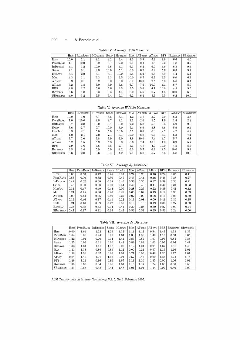
290 • A. Borodin et al.
Table IV. Average I (10) Measure
HITS PAGERANK INDEGREE SALSA HUBAVG MAX AT-MED AT-AVG BFS BAYESIAN SBAYESIAN
HITS 10.0 1.1 4.1 4.1 3.4 4.3 3.9 5.2 2.8 6.6 4.0PAGERANK 1.1 10.0 3.2 3.1 2.2 2.1 2.1 1.8 2.2 1.8 3.2INDEGREE 4.1 3.2 10.0 9.8 5.1 6.3 6.2 6.0 5.6 6.3 9.5SALSA 4.1 3.1 9.8 10.0 5.1 6.3 6.2 5.9 5.6 6.3 9.4HUBAVG 3.4 2.2 5.1 5.1 10.0 5.5 6.2 6.6 3.3 4.4 5.1MAX 4.3 2.1 6.3 6.3 5.5 10.0 8.7 6.7 5.5 6.0 6.2AT-MED 3.9 2.1 6.2 6.2 6.2 8.7 10.0 7.5 5.0 5.6 6.1AT-AVG 5.2 1.8 6.0 5.9 6.6 6.7 7.5 10.0 4.1 6.7 5.9BFS 2.8 2.2 5.6 5.6 3.3 5.5 5.0 4.1 10.0 4.5 5.5BAYESIAN 6.6 1.8 6.3 6.3 4.4 6.0 5.6 6.7 4.5 10.0 6.2SBAYESIAN 4.0 3.2 9.5 9.4 5.1 6.2 6.1 5.9 5.5 6.2 10.0
Table V. Average W I (10) Measure
HITS PAGERANK INDEGREE SALSA HUBAVG MAX AT-MED AT-AVG BFS BAYESIAN SBAYESIAN
HITS 10.0 1.0 3.7 3.6 3.3 4.2 3.7 5.2 2.9 6.3 3.6PAGERANK 1.0 10.0 2.8 2.7 2.1 2.1 2.0 1.5 1.6 1.4 2.8INDEGREE 3.7 2.8 10.0 9.7 5.0 7.2 6.8 5.9 5.6 5.9 9.6SALSA 3.6 2.7 9.7 10.0 5.0 7.1 6.9 5.8 5.6 5.9 9.4HUBAVG 3.3 2.1 5.0 5.0 10.0 5.1 6.0 6.3 2.7 4.2 4.9MAX 4.2 2.1 7.2 7.1 5.1 10.0 8.8 6.6 5.1 6.3 7.1AT-MED 3.7 2.0 6.8 6.9 6.0 8.8 10.0 7.4 4.7 5.7 6.8AT-AVG 5.2 1.5 5.9 5.8 6.3 6.6 7.4 10.0 4.0 6.9 5.7BFS 2.9 1.6 5.6 5.6 2.7 5.1 4.7 4.0 10.0 4.5 5.6BAYESIAN 6.3 1.4 5.9 5.9 4.2 6.3 5.7 6.9 4.5 10.0 5.8SBAYESIAN 3.6 2.8 9.6 9.4 4.9 7.1 6.8 5.7 5.6 5.8 10.0
Table VI. Average dr Distance
HITS PAGERANK INDEGREE SALSA HUBAVG MAX AT-MED AT-AVG BFS BAYESIAN SBAYESIAN
HITS 0.00 0.53 0.42 0.45 0.31 0.24 0.20 0.16 0.24 0.35 0.41PAGERANK 0.53 0.00 0.32 0.30 0.47 0.45 0.44 0.46 0.46 0.38 0.27INDEGREE 0.42 0.32 0.00 0.08 0.40 0.36 0.36 0.37 0.39 0.33 0.21SALSA 0.45 0.30 0.08 0.00 0.44 0.40 0.40 0.41 0.42 0.34 0.23HUBAVG 0.31 0.47 0.40 0.44 0.00 0.28 0.25 0.22 0.36 0.41 0.42MAX 0.24 0.45 0.36 0.40 0.28 0.00 0.07 0.13 0.19 0.30 0.33AT-MED 0.20 0.44 0.36 0.40 0.25 0.07 0.00 0.08 0.16 0.28 0.32AT-AVG 0.16 0.46 0.37 0.41 0.22 0.13 0.08 0.00 0.19 0.30 0.35BFS 0.24 0.46 0.39 0.42 0.36 0.19 0.16 0.19 0.00 0.27 0.33BAYESIAN 0.35 0.38 0.33 0.34 0.41 0.30 0.28 0.30 0.27 0.00 0.24SBAYESIAN 0.41 0.27 0.21 0.23 0.42 0.33 0.32 0.35 0.33 0.24 0.00
Table VII. Average d1 Distance
HITS PAGERANK INDEGREE SALSA HUBAVG MAX AT-MED AT-AVG BFS BAYESIAN SBAYESIAN
HITS 0.00 1.64 1.22 1.25 1.32 1.11 1.12 0.84 1.46 1.33 1.33PAGERANK 1.64 0.00 0.94 0.93 1.64 1.38 1.38 1.49 1.13 0.63 0.65INDEGREE 1.22 0.94 0.00 0.11 1.41 0.86 0.87 1.01 0.96 0.84 0.38SALSA 1.25 0.93 0.11 0.00 1.42 0.89 0.89 1.03 0.96 0.86 0.41HUBAVG 1.32 1.64 1.41 1.42 0.00 1.12 1.01 0.91 1.67 1.61 1.48MAX 1.11 1.38 0.86 0.89 1.12 0.00 0.21 0.57 1.19 1.16 1.01AT-MED 1.12 1.38 0.87 0.89 1.01 0.21 0.00 0.42 1.20 1.17 1.01AT-AVG 0.84 1.49 1.01 1.03 0.91 0.57 0.42 0.00 1.35 1.24 1.14BFS 1.46 1.13 0.96 0.96 1.67 1.19 1.20 1.35 0.00 1.06 0.99BAYESIAN 1.33 0.63 0.84 0.86 1.61 1.16 1.17 1.24 1.06 0.00 0.56SBAYESIAN 1.33 0.65 0.38 0.41 1.48 1.01 1.01 1.14 0.99 0.56 0.00
ACM Transactions on Internet Technology, Vol. 5, No. 1, February 2005.

Link Analysis Ranking: Algorithms, Theory and Experiments • 291
Table VIII. Query “Abortion”
HITS PAGERANK INDEGREE
1. (1.000) Priests for Life IndexURL:www.priestsforlife.org
1. (1.000) WCLA Feedback URL:www.janeylee.com/wcla
1. (1.000) prochoiceamerica.org :NARAL URL:www.naral.org
2. (0.997) National Right to LifeURL:www.nrlc.org
2. (0.911) Planned ParenthoodAction Ne URL:www.ppaction.org/ppaction/prof
2. (0.984) National Right to LifeURL:www.nrlc.org
3. (0.994) After Abortion:Information URL:www.afterabortion.org
3. (0.837) Welcome to theWestchester C URL:www.wcla.org
3. (0.969) Planned ParenthoodFederatio URL:www.plannedparenthood.org
4. (0.994) ProLifeInfo.orgURL:www.prolifeinfo.org
4. (0.714) Planned ParenthoodFederatio URL:www.plannedparenthood.org
4. (0.865) NAF—The Voice ofAbortion URL:www.prochoice.org
5. (0.990) Pregnancy CentersOnline URL:www.pregnancycenters.org
5. (0.633) GeneTree.com Page NotFound www.qksrv.net/click-1248625-91
5. (0.823) Priests for Life IndexURL:www.priestsforlife.org
6. (0.989) Human LifeInternational URL:www.hli.org
6. (0.630) Bible.com Prayer Roomwww.bibleprayerroom.com
6. (0.807) Pregnancy CentersOnline URL:www.pregnancycenters.org
7. (0.987) Abortion—Breast CancerLin URL:www.abortioncancer.com
7. (0.609) United StatesDepartment of URL:www.dhhs.gov
7. (0.740) ProLifeInfo.orgURL:www.prolifeinfo.org
8. (0.985) Abortion facts andinformati URL:www.abortionfacts.com
8. (0.538) Pregnancy CentersOnline URL:www.pregnancycenters.org
8. (0.734) After Abortion:Information URL:www.afterabortion.org
9. (0.981) Campaign Life CoalitionBrit URL:www.clcbc.org
9. (0.517) Bible.com Online Worldbible.com
9. (0.672) Abortion ClinicsOnLineURL:www.gynpages.com
10. (0.975) Empty title fieldwww.heritagehouse76.com
10. (0.516) National Organizationfor Wo URL:www.now.org
10. (0.625) Abortion—BreastCancer Lin URL:www.abortioncancer.com
HUBAVG MAX AT-MED
1. (1.000) prochoiceamerica.org :NARAL URL:www.naral.org
1. (1.000) prochoiceamerica.org :NARAL URL:www.naral.org
1. (1.000) prochoiceamerica.org :NARAL URL:www.naral.org
2. (0.935) Planned ParenthoodFederatio URL:www.plannedparenthood.org
2. (0.946) Planned ParenthoodFederatio URL:www.plannedparenthood.org
2. (0.933) Planned ParenthoodFederatio URL:www.plannedparenthood.org
3. (0.921) NAF—The Voice ofAbortion URL:www.prochoice.org
3. (0.918) National Right to LifeURL:www.nrlc.org
3. (0.837) NAF—The Voice ofAbortion URL:www.prochoice.org
4. (0.625) Abortion ClinicsOnLine URL:www.gynpages.com
4. (0.819) NAF—The Voice ofAbortion URL:www.prochoice.org
4. (0.717) National Right to LifeURL:www.nrlc.org
5. (0.516) FEMINIST MAJORITYFOUNDATION URL:www.feminist.org
5. (0.676) Priests for Life IndexURL:www.priestsforlife.org
5. (0.552) FEMINIST MAJORITYFOUNDATION URL:www.feminist.org
6. (0.484) The Alan GuttmacherInstitut URL:www.guttmacher.org
6. (0.624) Pregnancy CentersOnlineURL:www.pregnancycenters.org
6. (0.545) Abortion ClinicsOnLineURL:www.gynpages.com
7. (0.439) center forreproductive righ URL:www.crlp.org
7. (0.602) ProLifeInfo.orgURL:www.prolifeinfo.org
7. (0.538) The Alan GuttmacherInstitut URL:www.guttmacher.org
8. (0.416) The Religious Coalitionfor URL:www.rcrc.org
8. (0.557) Abortion ClinicsOnLine URL:www.gynpages.com
8. (0.523) center forreproductive righ URL:www.crlp.org
9. (0.415) National Organizationfor Wo URL:www.now.org
9. (0.551) After Abortion:Information URL:www.afterabortion.org
9. (0.518) Priests for Life IndexURL:www.priestsforlife.org
10. (0.408) Medical Students forChoice: URL:www.ms4c.org
10. (0.533) FEMINIST MAJORITYFOUNDATIONURL:www.feminist.org
10. (0.478) The Religious Coalitionfor URL:www.rcrc.org
ACM Transactions on Internet Technology, Vol. 5, No. 1, February 2005.

292 • A. Borodin et al.
Table VIII. Continue
AT-AVG BFS BAYESIAN
1. (1.000) National Right to LifeURL:www.nrlc.org
1. (1.000) National Right to LifeURL:www.nrlc.org
1. (7.04) National Right to LifeURL:www.nrlc.org
2. (0.905) Priests for Life IndexURL:www.priestsforlife.org
2. (0.930) Priests for Life IndexURL:www.priestsforlife.org
2. (6.79) Priests for Life IndexURL:www.priestsforlife.org
3. (0.844) ProLifeInfo.orgURL:www.prolifeinfo.org
3. (0.928) After Abortion:Information URL:www.afterabortion.org
3. (6.31) ProLifeInfo.orgURL:www.prolifeinfo.org
4. (0.785) Pregnancy CentersOnline URL:www.pregnancycenters.org
4. (0.905) Pro-life news andinformatio URL:www.all.org
4. (6.23) Pregnancy CentersOnline URL:www.pregnancycenters.org
5. (0.778) After Abortion:Information URL:www.afterabortion.org
5. (0.893) ProLifeInfo.orgURL:www.prolifeinfo.org
5. (6.09) After Abortion:Information URL:www.afterabortion.org
6. (0.777) prochoiceamerica.org :NARAL URL:www.naral.org
6. (0.869) Pregnancy CentersOnline URL:www.pregnancycenters.org
6. (5.67) Human Life InternationalURL:www.hli.org
7. (0.741) Human LifeInternational URL:www.hli.org
7. (0.860) Human LifeInternational URL:www.hli.org
7. (5.40) Abortion—Breast CancerLin URL:www.abortioncancer.com
8. (0.704) Planned ParenthoodFederatio URL:www.plannedparenthood.org
8. (0.852) Abortion facts andinformati URL:www.abortionfacts.com
8. (5.35) Abortion facts andinformati URL:www.abortionfacts.com
9. (0.683) Abortion facts andinformati URL:www.abortionfacts.com
9. (0.847) prochoiceamerica.org :NARAL URL:www.naral.org
9. (5.08) Campaign Life CoalitionBrit URL:www.clcbc.org
10. (0.677) Abortion—BreastCancer Lin URL:www.abortioncancer.com
10. (0.839) Planned ParenthoodFederatio URL:www.plannedparenthood.org
10. (4.36) Empty title fieldwww.heritagehouse76.com
Table IX. Query “Amusement Parks”
HITS PAGERANK INDEGREE
1. (1.000) Welcome to RENOLDIrides am URL:www.renoldi.com
1. (1.000) HONcode: Principleswww.hon.ch/HONcode/Conduct.htm
1. (1.000) HONcode: Principleswww.hon.ch/HONcode/Conduct.htm
2. (0.933) IAAPA URL:www.iaapa.org
2. (0.495) abc,Inflatable,tmoonwalk,moon www.adventure- bounce.com
2. (0.645) Empty title fieldURL:www.sixflags.com
3. (0.834) Knott’s URL:www.knotts.com
3. (0.335) Local Business ListingsBeac business.beachcomberii.com
3. (0.589) Busch GardensAdventure Park URL:www.buschgardens.com
4. (0.799) Traditional Amusementparks URL:www.tradition.cjb.net
4. (0.332) NAARSO NationalAssociation URL:www.naarso.com
4. (0.567) IAAPA URL:www.iaapa.org
5. (0.788) HUSS URL:www.hussrides.com
5. (0.332) AttorneyPages Helps YouFind attorneypages.com
5. (0.560) Free Legal Advice in 100+La freeadvice.com
6. (0.779) Empty title fieldURL:www.aimsintl.org
6. (0.332) Do It Yourself HomeImprovem doityourself.com
6. (0.560) AttorneyPages Helps YouFind attorneypages.com
7. (0.772) ScreamscapeURL:www.screamscape.com
7. (0.321) Theme Parks ClassifiedsURL:adlistings.themeparks.about.co
7. (0.560) Do It Yourself HomeImprovem doityourself.com
8. (0.770) REVERCHON : HOMEPAGE URL:www.reverchon.com
8. (0.317) FreeFind Site Searchsearch.freefind.com/find.html?
8. (0.532) ExpertPages.com—Books,Tap expert-pages.com/books.htm
9. (0.769) Empty title fieldURL:www.zierer.com
9. (0.315) Free Legal Advice in100+ La freeadvice.com
9. (0.489) Empty title fieldimgserv.adbutler.com/go2/;ID=1
10. (0.767) DEURL:www.drewexpo.com
10. (0.303) IAAPAURL:www.iaapa.org
10. (0.489) Empty title fieldimgserv.adbutler.com/go2/;ID=1
ACM Transactions on Internet Technology, Vol. 5, No. 1, February 2005.

Link Analysis Ranking: Algorithms, Theory and Experiments • 293
Table IX. Continue
HUBAVG MAX AT-MED
1. (1.000) HONcode: Principleswww.hon.ch/HONcode/Conduct.htm
1. (1.000) HONcode: Principleswww.hon.ch/HONcode/Conduct.htm
1. (1.000) AttorneyPages Helps YouFind attorneypages.com
2. (0.000) AttorneyPages Helps YouFind attorneypages.com
2. (0.000) Empty title fieldURL:www.sixflags.com
2. (1.000) Do It Yourself HomeImprovem doityourself.com
3. (0.000) Do It Yourself HomeImprovem doityourself.com
3. (0.000) Busch GardensAdventure Park URL:www.buschgardens.com
3. (0.987) Free Legal Advice in 100+La freeadvice.com
4. (0.000) Free Legal Advice in 100+La freeadvice.com
4. (0.000) Cedar PointAmusement Park, URL:www.cedarpoint.com
4. (0.949) ExpertPages.com—Books,Tap expert-pages.com/books.htm
5. (0.000) ExpertPages.com—Books,Tap expert-pages.com/books.htm
5. (0.000) IAAPA URL:www.iaapa.org
5. (0.866) Accidents Happen-Whyare L law.freeadvice.com/resources/c
6. (0.000) Accidents Happen-Whyare L law.freeadvice.com/resources/c
6. (0.000) Knott’s URL:www.knotts.com
6. (0.032) Expert Witness Directory|−F expertpages.com
7. (0.000) Empty title field imgserv.adbutler.com/go2/;ID=1
7. (0.000) Universal StudiosURL:www.usf.com
7. (0.017) Get Your Discount CardToday www.usaphonetime.com
8. (0.000) Empty title field imgserv.adbutler.com/go2/;ID=1
8. (0.000) Welcome to RENOLDIrides am URL:www.renoldi.com
8. (0.016) MapQuest: Homewww.mapquest.com
9. (0.000) Site Meter—Counter andSta s10.sitemeter.com/stats.asp?si
9. (0.000) Kennywood :America’s Finest URL:www.kennywood.com
9. (0.014) Adventure travel outdoorr www.outsidemag.com
10. (0.000) Empty title fieldimgserv.adbutler.com/go2/;ID=1
10. (0.000) Exhibits Collection –Amuse URL:www.learner.org/exhibits/parkp
10. (0.013) DisneylandResort—The offi URL:www.disneyland.com
AT-AVG BFS BAYESIAN
1. (1.000) AttorneyPages Helps YouFind attorneypages.com
1. (1.000) Knott’s URL:www.knotts.com
1. (1.88) Empty title fieldURL:www.sixflags.com
2. (1.000) Do It Yourself HomeImprovem doityourself.com
2. (0.910) Welcome to Gillette ShowsURL:www.gilletteshows.biz
2. (1.71) Welcome to RENOLDIrides am URL:www.renoldi.com
3. (0.995) Free Legal Advice in 100+La freeadvice.com
3. (0.885) Welcome to RENOLDIrides am URL:www.renoldi.com
3. (1.62) Busch GardensAdventure Park URL:www.buschgardens.com
4. (0.973) ExpertPages.com—Books,Tap expert-pages.com/books.htm
4. (0.884) IAAPA URL:www.iaapa.org
4. (1.60) Knott’s URL:www.knotts.com
AT-AVG BFS BAYESIAN
5. (0.900) Accidents Happen—Whyare L law.freeadvice.com/resources/c
5. (0.881) e-musementparkstore.com—Am URL:www.e-musementparkstore.com
5. (1.59) Cedar Point AmusementPark, URL:www.cedarpoint.com
6. (0.016) Expert Witness Directory|−F expertpages.com
6. (0.879) Great Adventure SourceURL:greatadventure.8m.com
6. (1.52) Kennywood : America’sFinest URL:www.kennywood.com
7. (0.012) Get Your Discount CardToday www.usaphonetime.com
7. (0.868) Web Page UnderConstruction www.carousel.org
7. (1.52) IAAPA URL:www.iaapa.org
8. (0.008) The Expert Pages—AboutAdv expertpages.com/about.htm
8. (0.854) amutechamutech.homestead.com
8. (1.46) Universal StudiosURL:www.usf.com
9. (0.008) Terms amp; Conditions atEx expertpages.com/conditions.htm
9. (0.850) Joyrides—AmusementPark an URL:www.joyrides.com
9. (1.44) Beachboardwalk.com:Californ URL:www.beachboardwalk.com
10. (0.008) Expert Pages PrivacyPolicy expertpages.com/privacy.htm
10. (0.849) Pharaohs LostKingdom Advent URL:www.pharaohslostkingdom.com
10. (1.35) LEGO.com Plug-inDownload URL:www.legolandca.com
ACM Transactions on Internet Technology, Vol. 5, No. 1, February 2005.

294 • A. Borodin et al.
Table X. Query “Classical Guitar”
HITS PAGERANK INDEGREE
1. (1.000) earlyromanticguitar.com URL:www.earlyromanticguitar.com
1. (1.000) Take Note PublishingLimited www.takenote.co.uk
1. (1.000) Guitar Alive-GuitarAlive—www.guitaralive.com
2. (0.927) Empty title field URL:classicalguitar.freehosting.ne
2. (0.724) Guitar music, guitarbooks a URL:www.booksforguitar.com
2. (0.895) earlyromanticguitar.com URL:www.earlyromanticguitar.com
3. (0.889) Adirondack Spruce.comURL:adirondackspruce.com
3. (0.588) Registry of GuitarTutors URL:www.registryofguitartutors.com
3. (0.889) Empty title fieldURL:www.guitarfoundation.org
4. (0.766) The Classical GuitarHomepag URL:www.ak-c.demon.nl
4. (0.528) Guitar Alive-GuitarAlive—www.guitaralive.com
4. (0.882) Hitsquad.com-MusiciansWeb URL:www.hitsquad.com
5. (0.732) Guitar Alive-GuitarAlive—www.guitaralive.com
5. (0.416) Hitsquad.com-MusiciansWeb URL:www.hitsquad.com
5. (0.850) Hitsquad Privacy Policywww.hitsquad.com/privacy.shtml
6. (0.681) Empty title fieldURL:www.guitarfoundation.org
6. (0.413) Hitsquad Privacy Policywww.hitsquad.com/privacy.shtml
6. (0.850) Advertising on HitsquadMusi www.hitsquad.com/advertising.s
7. (0.676) GUITAR REVIEWURL:www.guitarreview.com
7. (0.413) Advertising on HitsquadMusi www.hitsquad.com/advertising.s
7. (0.784) Adirondack Spruce.comURL:adirondackspruce.com
8. (0.644) Avi Afriat—Classicalguita URL:afriat.tripod.com
8. (0.387) Empty title field URL:www.guitarfoundation.org
8. (0.778) Empty title field URL:classicalguitar.freehosting.ne
9. (0.605) The Classical GuitarHome Pa URL:www.guitarist.com/cg/cg.htm
9. (0.343) Guitar Foundation ofAmerica URL:64.78.54.231
9. (0.765) Empty title field URL:www.vicnet.net.au/simieasyjamn
10. (0.586) Empty title fieldURL:www.duolenz.com
10. (0.322) Vivendi Universalwww.vivendiuniversal.com
10. (0.739) The Classical GuitarHomepag URL:www.ak-c.demon.nl
HUBAVG MAX AT-MED
1. (1.000) Hitsquad.com-MusiciansWeb URL:www.hitsquad.com
1. (1.000) Guitar Alive-GuitarAlive—www.guitaralive.com
1. (1.000) Hitsquad.com-MusiciansWeb URL:www.hitsquad.com
2. (0.995) Hitsquad Privacy Policywww.hitsquad.com/privacy.shtml
2. (0.619) earlyromanticguitar.com URL:www.earlyromanticguitar.com
2. (0.983) Hitsquad Privacy Policywww.hitsquad.com/privacy.shtml
3. (0.995) Advertising on HitsquadMusi www.hitsquad.com/advertising.s
3. (0.506) Empty title fieldURL:www.guitarfoundation.org
3. (0.983) Advertising on HitsquadMusi www.hitsquad.com/advertising.s
4. (0.856) Empty title field URL:www.vicnet.net.au/simieasyjamn
4. (0.451) Adirondack Spruce.comURL:adirondackspruce.com
4. (0.880) Empty title field URL:www.vicnet.net.au/simieasyjamn
5. (0.135) AMG All Music GuideURL:www.allmusic.com
5. (0.441) Empty title field URL:classicalguitar.freehosting.ne
5. (0.205) AMG All Music GuideURL:www.allmusic.com
6. (0.132) Free Music Download,MP3 Mus ubl.com
6. (0.378) GUITAR REVIEWURL:www.guitarreview.com
6. (0.193) Free Music Download,MP3 Mus ubl.com
7. (0.130) 2000 Guitars DatabaseURL:dargo.vicnet.net.au/guitar/lis
7. (0.377) The Classical GuitarHomepag URL:www.ak-c.demon.nl
7. (0.169) 2000 Guitars DatabaseURL:dargo.vicnet.net.au/guitar/lis
8. (0.115) Guitar Alive-GuitarAlive—www.guitaralive.com
8. (0.371) The Classical GuitarHome Pa URL:www.guitarist.com/cg/cg.htm
8. (0.132) Guitar Alive-GuitarAlive—www.guitaralive.com
9. (0.096) CDNOW www.cdnow.com/from=sr-767167
9. (0.336) Hitsquad.com-MusiciansWeb URL:www.hitsquad.com
9. (0.129) CDNOW www.cdnow.com/from=sr-767167
10. (0.056) OLGA—The On-LineGuitar Ar URL:www.olga.net
10. (0.312) Hitsquad Privacy Policywww.hitsquad.com/privacy.shtml
10. (0.082) OLGA—The On-LineGuitar Ar URL:www.olga.net
AT-AVG BFS BAYESIAN
1. (1.000) Hitsquad.com-MusiciansWeb URL:www.hitsquad.com
1. (1.000) Empty title field URL:classicalguitar.freehosting.ne
1. (3.66) earlyromanticguitar.com URL:www.earlyromanticguitar.com
2. (0.986) Hitsquad Privacy Policywww.hitsquad.com/privacy.shtml
2. (0.991) earlyromanticguitar.com URL: www.earlyromanticguitar.com
2. (3.54) Empty title field URL:classicalguitar.freehosting.ne
ACM Transactions on Internet Technology, Vol. 5, No. 1, February 2005.

Link Analysis Ranking: Algorithms, Theory and Experiments • 295
Table X. Continue
3. (0.986) Advertising on HitsquadMusi www.hitsquad.com/advertising.s
3. (0.974) Adirondack Spruce.comURL:adirondackspruce.com
3. (3.53) Adirondack Spruce.comURL:adirondackspruce.com
4. (0.906) Empty title field URL:www.vicnet.net.au/simieasyjamn
4. (0.962) Empty title fieldURL:www.guitarfoundation.org
4. (3.42) Hitsquad.com—MusiciansWeb URL:www.hitsquad.com
5. (0.210) AMG All Music GuideURL:www.allmusic.com
5. (0.945) Guitar Alive-GuitarAlive—www.guitaralive.com
5. (3.38) Guitar Alive-GuitarAlive—www.guitaralive.com
6. (0.199) Free Music Download,MP3 Mus ubl.com
6. (0.933) The Classical GuitarHomepag URL:www.ak-c.demon.nl
6. (3.33) Empty title fieldURL:www.guitarfoundation.org
7. (0.179) 2000 Guitars DatabaseURL:dargo.vicnet.net.au/guitar/lis
7. (0.917) The Classical GuitarHome Pa URL:www.guitarist.com/cg/cg.htm
7. (3.33) Hitsquad Privacy Policywww.hitsquad.com/privacy.shtml
8. (0.135) CDNOW www.cdnow.com/from=sr-767167
8. (0.898) Avi Afriat—Classicalguita URL:afriat.tripod.com
8. (3.33) Advertising on HitsquadMusi www.hitsquad.com/advertising.s
9. (0.122) Guitar Alive-GuitarAlive—www.guitaralive.com
9. (0.889) GUITAR REVIEWURL:www.guitarreview.com
9. (3.27) The Classical GuitarHomepag URL:www.ak-c.demon.nl
10. (0.080) OLGA—The On-LineGuitar Ar URL:www.olga.net
10. (0.881) Empty title fieldURL:www.duolenz.com
10. (3.25) GUITAR REVIEWURL:www.guitarreview.com
ACKNOWLEDGMENTS
We would like to thank Alberto Mendelzon, Renee Miller, Ken Sevcik, KenJackson, Jon Kleinberg, Sam Roweis, Ronald Fagin, Ronny Lempel, ShlomoMoran, and the anonymous reviewers for valuable comments and corrections.We would also like to thank all the people who participated in the online surveyfor determining the relevance of the search results.
REFERENCES
ACHLIOPTAS, D., FIAT, A., KARLIN, A., AND MCSHERRY, F. 2001. Web search through hub synthesis.In Proceedings of the 42nd Foundation of Computer Science (FOCS 2001). Las Vegas, NY.
ANDRITSOS, P., TSAPARAS, P., MILLER, R., AND SEVCIK, K. 2003. LIMBO: Scalable clustering of cate-gorical data. Submitted for publication.
AZAR, Y., FIAT, A., KARLIN, A., MCSHERRY, F., AND SAIA, J. 2001. Spectral analysis of data. In Proceed-ings of the 33rd Symposium on Theory of Computing (STOC 2001). Hersonissos, Crete, Greece.
BERNARDO, J. AND SMITH, A. 1994. Bayesian Theory. John Wiley & Sons, Chichester, England.BHARAT, K. AND HENZINGER, M. R. 1998. Improved algorithms for topic distillation in a hyperlinked
environment. In Research and Development in Information Retrieval. 104–111.BHARAT, K. AND MIHAILA, G. A. 2001. When experts agree: Using non-affiliated experts to rank
popular topics. In Proceedings of the 10th International World Wide Web Conference.BIANCHINI, M., GORI, M., AND SCARSELLI, F. 2002. PageRank: A circuital analysis. In Proceedings
of the 11th International Word Wide Web Conference (WWW 2002). Poster Session. Hawai.BORODIN, A., ROBERTS, G. O., ROSENTHAL, J. S., AND TSAPARAS, P. 2001. Finding authorities and hubs
from link structures on the World Wide Web. In Proceedings of the 10th International World WideWeb Conference. Hong Kong.
BRIN, S. AND PAGE, L. 1998. The anatomy of a large-scale hypertextual Web search engine. InProceedings of the 7th International World Wide Web Conference. Brisbane, Australia.
BRODER, A. 2002. Web searching technology overview. In Advanced School and Workshop onModels and Algorithms for the World Wide Web. Udine, Italy.
CHAKRABARTI, S., DOM, B., GIBSON, D., KLEINBERG, J., RAGHAVAN, P., AND RAJAGOPALAN, S. 1998. Auto-matic resource compilation by analysing hyperlink structure and associated text. In Proceedingsof the 7th International World Wide Web Conference.
CHIEN, S., DWORK, C., KUMAR, R., SIMON, D., AND SIVAKUMAR, D. 2002. Towards exploiting linkevolution. In Workshop on Algorithms for the Web. Vancuver, Canada.
ACM Transactions on Internet Technology, Vol. 5, No. 1, February 2005.

296 • A. Borodin et al.
COHN, D. AND CHANG, H. 2000. Learning to probabilistically identify authoritative documents.In Proceedings of the 17th International Conference on Machine Learning. Stanford University,167–174.
DAVISON, B. 2000. Recognizing nepotistic links on the web. In AAAI-2000 Workshop on ArtificialIntelligence for Web Search. AAAI Press, Austin, TX.
DEMPSTER, A., LAIRD, N., AND RUBIN, D. 1977. Maximum likelihood from incomplete data via theEM algorithm. J. Roy. Statist. Soc., Series B, 39, 1–38.
DIACONIS, P. AND GRAHAM, R. 1977. Spearman’s footrule as a measure of disarray. J. Roy. Statist.Soc. 39, 2, 262–268.
DRINEAS, P., FRIEZE, A., KANNAN, R., VEMPALA, S., AND VINAY, V. 1999. Clustering in large graphsand matrices. In ACM-SIAM Symposium on Discrete Algorithms (SODA).
DWORK, C., KUMAR, R., NAOR, M., AND SIVAKUMAR, D. 2001. Rank aggregation methods for the Web.In Proceedings of the 10th International World Wide Web Conference. Hong Kong.
FAGIN, R., KUMAR, R., MAHDIAN, M., SIVAKUMAR, D., AND VEE, E. 2004. Comparing and aggregatingrankings with ties. In Symposium on Principles of Database Systems (PODS).
FAGIN, R., KUMAR, R., AND SIVAKUMAR, D. 2003. Comparing top k lists. In Proceedings of the ACM-SIAM Symposium on Discrete Algorithms (SODA).
GIBSON, D., KLEINBERG, J., AND RAGHAVAN, P. 1998. Inferring Web communities from link topology.In Proceedings of 9th ACM Conference on Hypertext and Hypermedia.
GILKS, W., RICHARDSON, S., AND SPIEGELHALTER, D. 1996. Markov Chain Monte Carlo in practice.Chapman and Hall, London.
HAVELIWALA, T. H. 2002. Topic sensitive Page Rank. In Proceedings of the 11th International WordWide Web Conference (WWW 2002). Hawai.
HOFMANN, T. 1999. Probabilistic latent semantic analysis. In Proceedings of Uncertainty in Arti-ficial Intelligence, UAI’99. Stockholm, Sweden.
HOFMANN, T. 2000. Learning probabilistic models of the Web. In Proceedings of the 23rd Interna-tional Conference on Research and Development in Information Retrieval (ACM SIGIR’00).
JANSEN, B. J., SPINK, A., BATEMAN, J., AND SARACEVIC, T. 1998. Real Life Information Retrieval: AStudy of User Queries on the Web. ACM SIGIR Forum 32, 5–17.
JEN, G. AND WIDOM, J. 2003. Scaling personalized Web search. In Proceedings of the 12th Inter-national World Wide Wed Conference(WWW2003). Budapest, Hungary.
KATZ, L. 1953. A new status index derived from sociometric analysis. Psychometrika 18, 39–43.KENDALL, M. G. 1970. Rank Correlation Methods. Griffin, London, UK.KLEINBERG, J. 1998. Authoritative sources in a hyperlinked environment. In Proceedings of the
Ninth Annual ACM-SIAM Symposium on Discrete Algorithms. 668–677.KLEINBERG, J. 1999. Authoritative sources in a hyperlinked environment. J. ACM 46.LEE, H. C. AND BORODIN, A. 2003. Perturbation of the hyperlinked environment. In Proceedings
of the 9th International Computing and Combinatorics Conference.LEMPEL, R. AND MORAN, S. 2000. The stochastic approach for link-structure analysis (SALSA) and
the TKC effect. In Proceedings of the 9th International World Wide Web Conference.LEMPEL, R. AND MORAN, S. 2001. Rank stability and rank similarity of Web link-based ranking
algorithms. Tech. Rep. CS-2001-22. Technion—Israel Institute of Technology.LEMPEL, R. AND MORAN, S. 2003. Rank stability and rank similarity of Web link-based ranking al-
gorithms. In 2nd Workshop on Algorithms and Models for the Web-Graph (WAW2003). Budapest,Hungary.
LIN, J. 1991. Divergence measures based on the Shannon entropy. Mach. Learn. 37, 1, 145–151.MARCHIORI, M. 1997. The quest for correct information on Web: Hyper search engines. In Pro-
ceedings of the 6th International World Wide Web Conference.MENDELZON, A. AND RAFIEI, D. 2000. What do the neighbours think? Computing Web page repu-
tations. IEEE Data Eng. Bull. 23, 3, 9–16.NG, A. Y., ZHENG, A. X., AND JORDAN, M. I. 2001a. Link analysis, eigenvectors, and stability.
In Proceedings of the International Joint Conference on Artificial Intelligence (IJCAI). Seattle,Washington.
NG, A. Y., ZHENG, A. X., AND JORDAN, M. I. 2001b. Stable algorithms for link analysis. In Proceed-ings of the 24th International Conference on Research and Development in Information Retrieval(SIGIR 2001). New York, NY.
ACM Transactions on Internet Technology, Vol. 5, No. 1, February 2005.

Link Analysis Ranking: Algorithms, Theory and Experiments • 297
PAGE, L., BRIN, S., MOTWANI, R., AND WINOGRAD, T. 1998. The PageRank citation ranking: Bringingorder to the web. Tech. rep. Stanford Digital Library Technologies Project.
RAFIEI, D. AND MENDELZON, A. 2000. What is this page known for? Computing Web page rep-utations. In Proceedings of the 9th International World Wide Web Conference. Amsterdam,Netherlands.
RICHARDSON, M. AND DOMINGOS, P. 2002. The intelligent surfer: Probabilistic combination of linkand content information in PageRank. In Advances in Neural Information Processing Systems(NIPS) 14.
ROBERTS, G. AND ROSENTHAL, J. 1998. Markov chain Monte Carlo: Some practical implications oftheoretical results (with discussion). Canadian J. Statist. 26, 5–31.
ROBERTS, G. O. AND ROSENTHAL, J. S. 2003. Downweighting tightly knit communities in WorldWide Web rankings. Adv. Appl. Statist. 3, 199–216.
SILVERSTEIN, C., HENZINGER, M., MARAIS, H., AND MORICZ, M. 1998. Analysis of a very large AltaVistaquery log. Tech. Rep. 1998-014. Digital SRC.
SLONIM, N. AND TISHBY, N. 1999. Agglomerative Information Bottleneck. In Advances in NeuralInformation Processing Systems (NIPS). Breckenridge, CO.
SMITH, A. AND ROBERTS, G. 1993. Bayesian computation via the Gibbs sampler and related Markovchain Monte Carlo methods (with discussion). J. Roy. Statist. Soc., Series B, 55, 3–24.
TIERNEY, L. 1994. Markov chains for exploring posterior distributions (with discussion). Ann.Statist. 22, 1701–1762.
TISHBY, N., PEREIRA, F. C., AND BIALEK, W. 1999. The Information Bottleneck method. In 37thAnnual Allerton Conference on Communication, Control and Computing. Urban-Champaign, IL.
TOMLIN, J. A. 2003. A new paradigm for ranking pages on the World Wide Web. In Proceedingsof the 12th International World Wide Wed Conference (WWW2003). Budapest, Hungary.
TSAPARAS, P. 2004a. Link analysis ranking. Ph.D. thesis, University of Toronto.TSAPARAS, P. 2004b. Using non-linear dynamical systems for Web searching and ranking. In
Symposium on Principles of Database Systems (PODS). Paris, France.
Received November 2001; revised March 2004; accepted April 2004
ACM Transactions on Internet Technology, Vol. 5, No. 1, February 2005.


![Link Analysis Ranking: Algorithms, Theory, and Experiments · 234 • A. Borodin et al. algorithm is the adjacency matrix W of the graph G, where W[i, j] = 1ifthere is a link from](https://img.dokumen.tips/doc/110x75/5ed090d56d95d97b48122c83/link-analysis-ranking-algorithms-theory-and-experiments-234-a-a-borodin-et.jpg)


