Embed Size (px)
Citation preview
Linearized Polynomial Modules and their Application to Network Coding
Linearized Polynomial Modules and theirApplication to Network Coding
Anna-Lena Horlemann-Trautmann
Algorithmics LaboratoryEPF Lausanne, Switzerland
October 18th, 2016Clemson University
Linearized Polynomial Modules and their Application to Network Coding
Linearized Polynomials
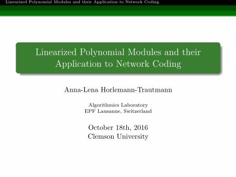
1 Linearized PolynomialsThe Ring Lq(x, q
m)Modules over Lq(x, q
m)
2 Network Coding and Gabidulin CodesIntroductionGabidulin Codes and Interpolation Decoding
3 Summary and Conclusion

Linearized Polynomial Modules and their Application to Network Coding
Linearized Polynomials
The Ring Lq(x, qm)
Brief Recap of Finite Fields
Fq exists (uniquely) for q = pr, p prime
Fp∼= Zp
Fqm∼= Fq[α], α root of irreducible polynomial of degree m
Freshman’s Dream: (a+ b)q = aq + bq for a, b ∈ Fqm
aq = a for a ∈ Fq ≤ Fqm
1 / 35

Linearized Polynomial Modules and their Application to Network Coding
Linearized Polynomials
The Ring Lq(x, qm)
Definition
A (q-)linearized polynomial is of the form
f(x) =
n∑i=0
aixqi
for ai ∈ Fqm . If an ̸= 0, n is called the q-degree of f(x).
Theorem
The set Lq(x, qm) of all q-linearized polynomials over Fqm forms
a non-commutative ring, equipped with the normal addition +and composition (symbolic multiplication) ◦.
2 / 35

Linearized Polynomial Modules and their Application to Network Coding
Linearized Polynomials
The Ring Lq(x, qm)
Example in L3(x, 32)
F32∼= F3[α], where α2 + 1 = 0
(2x3 + x) + (αx9 + x3) = αx9 + x
(2x3 + x) ◦ (αx9 + x3) = 2(αx9 + x3)3 + (αx9 + x3)= 2α3x27 + (2 + α)x9 + x3 = αx27 + (2 + α)x9 + x3
(αx9 + x3) ◦ (2x3 + x) = α(2x3 + x)9 + (2x3 + x)3
= 2αx27 + (2 + α)x9 + x3
3 / 35
Linearized Polynomial Modules and their Application to Network Coding
Linearized Polynomials
The Ring Lq(x, qm)
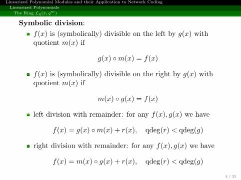
Symbolic division:
f(x) is (symbolically) divisible on the left by g(x) withquotient m(x) if
g(x) ◦m(x) = f(x)
f(x) is (symbolically) divisible on the right by g(x) withquotient m(x) if
m(x) ◦ g(x) = f(x)
left division with remainder: for any f(x), g(x) we have
f(x) = g(x) ◦m(x) + r(x), qdeg(r) < qdeg(g)
right division with remainder: for any f(x), g(x) we have
f(x) = m(x) ◦ g(x) + r(x), qdeg(r) < qdeg(g)
4 / 35

Linearized Polynomial Modules and their Application to Network Coding
Linearized Polynomials
The Ring Lq(x, qm)
Theorem
A linearized polynomial f(x) ∈ Lq(x, qm) is an Fq-linear map. If
qdeg(f) = k, then ker(f) is a k-dimensional Fq-vector space(over some extension field).
Example in L3(x, 32)
f(x) = x3 + 2α2x
f(λx+µy) = (λx+µy)3+2α2(λx+µy) = λx3+µy3+2α2λx+2α2µy = λ(x3 + 2α2x) + µ(y3 + 2α2y) = λf(x) + µf(y),for λ, µ ∈ F3
ker(f) = {0, α, 2α}
5 / 35
Linearized Polynomial Modules and their Application to Network Coding
Linearized Polynomials
The Ring Lq(x, qm)
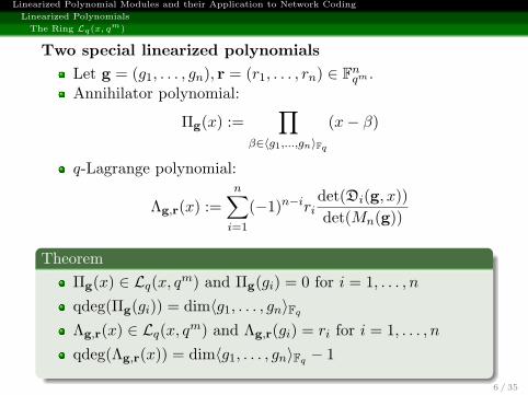
Two special linearized polynomials
Let g = (g1, . . . , gn), r = (r1, . . . , rn) ∈ Fnqm .
Annihilator polynomial:
Πg(x) :=∏
β∈⟨g1,...,gn⟩Fq
(x− β)
q-Lagrange polynomial:
Λg,r(x) :=n∑
i=1
(−1)n−iridet(Di(g, x))
det(Mn(g))
Theorem
Πg(x) ∈ Lq(x, qm) and Πg(gi) = 0 for i = 1, . . . , n
qdeg(Πg(gi)) = dim⟨g1, . . . , gn⟩Fq
Λg,r(x) ∈ Lq(x, qm) and Λg,r(gi) = ri for i = 1, . . . , n
qdeg(Λg,r(x)) = dim⟨g1, . . . , gn⟩Fq − 1
6 / 35

Linearized Polynomial Modules and their Application to Network Coding
Linearized Polynomials
Modules over Lq(x, qm)
1 Linearized PolynomialsThe Ring Lq(x, q
m)Modules over Lq(x, q
m)
2 Network Coding and Gabidulin CodesIntroductionGabidulin Codes and Interpolation Decoding
3 Summary and Conclusion

Linearized Polynomial Modules and their Application to Network Coding
Linearized Polynomials
Modules over Lq(x, qm)
Left Module Lq(x, qm)ℓ
for fi(x) ∈ Lq(x, qm), the elements of Lq(x, q
m)ℓ are
f := [f1(x) . . . fℓ(x)] =
ℓ∑i=1
fi(x)ei
for h(x) ∈ Lq(x, qm)
h(x) ◦ f := [h(f1(x)) . . . h(fℓ(x))] =
ℓ∑i=1
h(fi(x))ei.
Definition
A subset M ⊆ Lq(x, qm)ℓ is a (left) submodule of Lq(x, q
m)ℓ if itis closed under addition and composition with Lq(x, q
m) on theleft.
7 / 35

Linearized Polynomial Modules and their Application to Network Coding
Linearized Polynomials
Modules over Lq(x, qm)
Definition
Consider f (1), . . . , f (s) ∈ Lq(x, qm)ℓ. f (1), . . . , f (s) are linearly
independent if for any a1(x), . . . , as(x) ∈ Lq(x, qm)
s∑i=1
ai(x) ◦ f (i) = [ 0 . . . 0 ] =⇒ a1(x) = · · · = as(x) = 0.
A generating set of a submodule M ⊆ Lq(x, qm)ℓ is called a
basis of M if all its elements are linearly independent.
8 / 35

Linearized Polynomial Modules and their Application to Network Coding
Linearized Polynomials
Modules over Lq(x, qm)
Monomials
Notation: [i] := qi
The monomials of f = [f1(x) . . . fℓ(x)] are of the formx[k]ei for all k such that fik ̸= 0.
A monomial order < on Lq(x, qm)ℓ is a total order on
Lq(x, qm)ℓ, analogous to normal polynomial ring.
The (k1, . . . , kℓ)-weighted term-over-position monomialorder is defined as
x[i1]ej1 <(k1,...,kℓ) x[i2]ej2 : ⇐⇒
i1 + kj1 < i2 + kj2 or [i1 + kj1 = i2 + kj2 and j1 < j2].
9 / 35

Linearized Polynomial Modules and their Application to Network Coding
Linearized Polynomials
Modules over Lq(x, qm)
Definition
For any monomial order we define the following:
the leading monomial lm(f) = x[i1]ej1 is the greatestmonomial of f .
the leading position lpos(f) = j1 is the vector coordinate ofthe leading monomial.
the leading term lt(f) = fj1,i1x[i1]ej1 is the complete term of
the leading monomial.
The (k1, . . . , kℓ)-weighted q-degree of [f1(x) . . . fℓ(x)] is definedas max{ki + qdeg(fi(x)) | i = 1, . . . , ℓ}.
10 / 35
Linearized Polynomial Modules and their Application to Network Coding
Linearized Polynomials
Modules over Lq(x, qm)
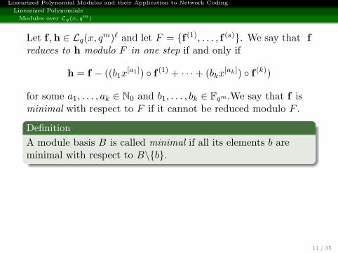
Let f ,h ∈ Lq(x, qm)ℓ and let F = {f (1), . . . , f (s)}. We say that f
reduces to h modulo F in one step if and only if
h = f − ((b1x[a1]) ◦ f (1) + · · ·+ (bkx
[ak]) ◦ f (k))
for some a1, . . . , ak ∈ N0 and b1, . . . , bk ∈ Fqm .We say that f isminimal with respect to F if it cannot be reduced modulo F .
Definition
A module basis B is called minimal if all its elements b areminimal with respect to B\{b}.
Theorem
Let B be a basis of a module M ⊆ Lq(x, qm)ℓ. Then B is a
minimal basis if and only if all leading positions of the elementsof B are distinct.
11 / 35

Linearized Polynomial Modules and their Application to Network Coding
Linearized Polynomials
Modules over Lq(x, qm)
Example in L3(x, 32)2
consider (1, 2)-weighted TOP order and
f = [x3 + x αx3], g = [2x9 + x3 2x]
qdeg(1,2)(f) = max(1 + 1, 1 + 2) = 3,qdeg(1,2)(g) = max(2 + 1, 0 + 2) = 3
lpos(f) = 2, lpos(g) = 1
lm(f) = [0 x3], lm(g) = [x9 0]
lt(f) = [0 αx3], lt(g) = [2x9 0]
=⇒ {f ,g} is a minimal basis of
rowspan
[x3 + x αx3
2x9 + x3 2x
]
12 / 35
Linearized Polynomial Modules and their Application to Network Coding
Linearized Polynomials
Modules over Lq(x, qm)
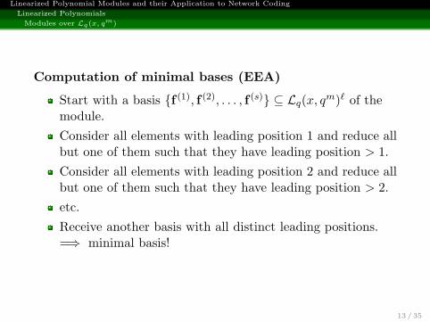
Computation of minimal bases (EEA)
Start with a basis {f (1), f (2), . . . , f (s)} ⊆ Lq(x, qm)ℓ of the
module.
Consider all elements with leading position 1 and reduce allbut one of them such that they have leading position > 1.
Consider all elements with leading position 2 and reduce allbut one of them such that they have leading position > 2.
etc.
Receive another basis with all distinct leading positions.=⇒ minimal basis!
13 / 35

Linearized Polynomial Modules and their Application to Network Coding
Linearized Polynomials
Modules over Lq(x, qm)
Example in L3(x, 32)2
f = [2x27 + x9 + x3 + x (α+ 2)x3], g = [2x9 + x3 2x]
both have leading position 1 in (1, 2)-weighted order
compute h = f − x3 ◦ g = [x3 + x αx3]
h has leading position 2
{g,h} is minimal basis of ⟨f ,g⟩
14 / 35
Linearized Polynomial Modules and their Application to Network Coding
Linearized Polynomials
Modules over Lq(x, qm)
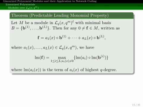
Theorem (Predictable Leading Monomial Property)
Let M be a module in Lq(x, qm)ℓ with minimal basis
B = {b(1), . . . ,b(L)}. Then for any 0 ̸= f ∈ M , written as
f = a1(x) ◦ b(1) + · · ·+ aL(x) ◦ b(L),
where a1(x), . . . , aL(x) ∈ Lq(x, qm), we have
lm(f) = max1≤i≤L;ai(x) ̸=0
{lm(ai) ◦ lm(b(i))}
where lm(ai(x)) is the term of ai(x) of highest q-degree.
Corollary
The leading positions and weighted q-degrees of elements of twodistinct minimal bases for the same module in Lq(x, q
m)ℓ haveto be the same. =⇒ cardinalities of minimal bases are equal
15 / 35

Linearized Polynomial Modules and their Application to Network Coding
Linearized Polynomials
Modules over Lq(x, qm)
Theorem (Predictable Leading Monomial Property)
Let M be a module in Lq(x, qm)ℓ with minimal basis
B = {b(1), . . . ,b(L)}. Then for any 0 ̸= f ∈ M , written as
f = a1(x) ◦ b(1) + · · ·+ aL(x) ◦ b(L),
where a1(x), . . . , aL(x) ∈ Lq(x, qm), we have
lm(f) = max1≤i≤L;ai(x) ̸=0
{lm(ai) ◦ lm(b(i))}
where lm(ai(x)) is the term of ai(x) of highest q-degree.
Corollary
The leading positions and weighted q-degrees of elements of twodistinct minimal bases for the same module in Lq(x, q
m)ℓ haveto be the same. =⇒ cardinalities of minimal bases are equal
15 / 35
Linearized Polynomial Modules and their Application to Network Coding
Linearized Polynomials
Modules over Lq(x, qm)
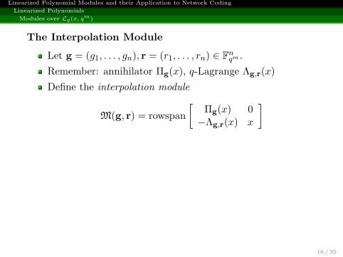
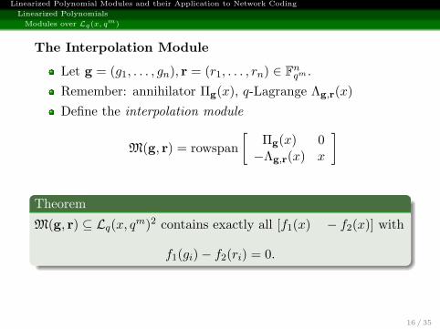
The Interpolation Module
Let g = (g1, . . . , gn), r = (r1, . . . , rn) ∈ Fnqm .
Remember: annihilator Πg(x), q-Lagrange Λg,r(x)
Define the interpolation module
M(g, r) = rowspan
[Πg(x) 0
−Λg,r(x) x
]
Theorem
M(g, r) ⊆ Lq(x, qm)2 contains exactly all [f1(x) − f2(x)] with
f1(gi)− f2(ri) = 0.
=⇒ minimal basis of M(g, r) can be computed in Oqm(n3)
operations with EEA
16 / 35
Linearized Polynomial Modules and their Application to Network Coding
Linearized Polynomials
Modules over Lq(x, qm)
The Interpolation Module
Let g = (g1, . . . , gn), r = (r1, . . . , rn) ∈ Fnqm .
Remember: annihilator Πg(x), q-Lagrange Λg,r(x)
Define the interpolation module
M(g, r) = rowspan
[Πg(x) 0
−Λg,r(x) x
]
Theorem
M(g, r) ⊆ Lq(x, qm)2 contains exactly all [f1(x) − f2(x)] with
f1(gi)− f2(ri) = 0.
=⇒ minimal basis of M(g, r) can be computed in Oqm(n3)
operations with EEA
16 / 35

Linearized Polynomial Modules and their Application to Network Coding
Network Coding and Gabidulin Codes
Introduction
1 Linearized PolynomialsThe Ring Lq(x, q
m)Modules over Lq(x, q
m)
2 Network Coding and Gabidulin CodesIntroductionGabidulin Codes and Interpolation Decoding
3 Summary and Conclusion

Linearized Polynomial Modules and their Application to Network Coding
Network Coding and Gabidulin Codes
Introduction
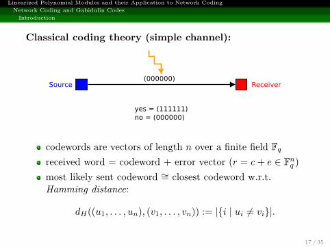
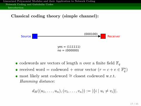
Classical coding theory (simple channel):
codewords are vectors of length n over a finite field Fq
received word = codeword + error vector (r = c+ e ∈ Fnq )
most likely sent codeword ∼= closest codeword w.r.t.Hamming distance:
dH((u1, . . . , un), (v1, . . . , vn)) := |{i | ui ̸= vi}|.
17 / 35
Linearized Polynomial Modules and their Application to Network Coding
Network Coding and Gabidulin Codes
Introduction
Classical coding theory (simple channel):
codewords are vectors of length n over a finite field Fq
received word = codeword + error vector (r = c+ e ∈ Fnq )
most likely sent codeword ∼= closest codeword w.r.t.Hamming distance:
dH((u1, . . . , un), (v1, . . . , vn)) := |{i | ui ̸= vi}|.
17 / 35

Linearized Polynomial Modules and their Application to Network Coding
Network Coding and Gabidulin Codes
Introduction
Multicast Channel
All receivers want to receive the same information.
18 / 35

Linearized Polynomial Modules and their Application to Network Coding
Network Coding and Gabidulin Codes
Introduction
Example (Butterfly Network)
Linearly combining is better than forwarding:
R2
R1
a
a
a
aa
b b
b
a
R1 receives only a, R2 receives a and b.
Forwarding: need 2 transmissions to transmit a, b to bothreceivers
Linearly combining: need 1 transmission to transmit a, b toboth receivers
19 / 35

Linearized Polynomial Modules and their Application to Network Coding
Network Coding and Gabidulin Codes
Introduction
Example (Butterfly Network)
Linearly combining is better than forwarding:
R2
R1
a
a
a
a+ba+b
b b
b
a+b
R1 and R2 can both recover a and b with one operation.
Forwarding: need 2 transmissions to transmit a, b to bothreceivers
Linearly combining: need 1 transmission to transmit a, b toboth receivers
19 / 35

Linearized Polynomial Modules and their Application to Network Coding
Network Coding and Gabidulin Codes
Introduction
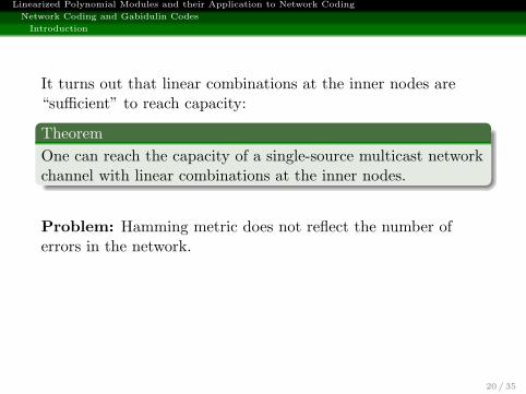
It turns out that linear combinations at the inner nodes are“sufficient” to reach capacity:
Theorem
One can reach the capacity of a single-source multicast networkchannel with linear combinations at the inner nodes.
Problem: Hamming metric does not reflect the number oferrors in the network.Solution: Use metric space (Fm×n
q , dR),
dR(A,B) = rank(A−B).
20 / 35
Linearized Polynomial Modules and their Application to Network Coding
Network Coding and Gabidulin Codes
Introduction
It turns out that linear combinations at the inner nodes are“sufficient” to reach capacity:
Theorem
One can reach the capacity of a single-source multicast networkchannel with linear combinations at the inner nodes.
Problem: Hamming metric does not reflect the number oferrors in the network.
Solution: Use metric space (Fm×nq , dR),
dR(A,B) = rank(A−B).
20 / 35

Linearized Polynomial Modules and their Application to Network Coding
Network Coding and Gabidulin Codes
Introduction
It turns out that linear combinations at the inner nodes are“sufficient” to reach capacity:
Theorem
One can reach the capacity of a single-source multicast networkchannel with linear combinations at the inner nodes.
Problem: Hamming metric does not reflect the number oferrors in the network.Solution: Use metric space (Fm×n
q , dR),
dR(A,B) = rank(A−B).
20 / 35
Linearized Polynomial Modules and their Application to Network Coding
Network Coding and Gabidulin Codes
Introduction
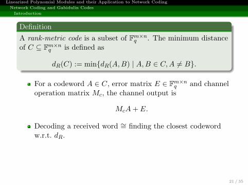
Definition
A rank-metric code is a subset of Fm×nq . The minimum distance
of C ⊆ Fm×nq is defined as
dR(C) := min{dR(A,B) | A,B ∈ C,A ̸= B}.
For a codeword A ∈ C, error matrix E ∈ Fm×nq and channel
operation matrix Mc, the channel output is
McA+ E.
Decoding a received word ∼= finding the closest codewordw.r.t. dR.
The error correction capability of C is (dR(C)− 1)/2.
The transmission rate of C is logq(|C|)/(mn).
We can use Fm×nq
∼= Fnqm and define C ⊆ Fn
qm .
21 / 35

Linearized Polynomial Modules and their Application to Network Coding
Network Coding and Gabidulin Codes
Introduction
Definition
A rank-metric code is a subset of Fm×nq . The minimum distance
of C ⊆ Fm×nq is defined as
dR(C) := min{dR(A,B) | A,B ∈ C,A ̸= B}.
For a codeword A ∈ C, error matrix E ∈ Fm×nq and channel
operation matrix Mc, the channel output is
McA+ E.
Decoding a received word ∼= finding the closest codewordw.r.t. dR.
The error correction capability of C is (dR(C)− 1)/2.
The transmission rate of C is logq(|C|)/(mn).
We can use Fm×nq
∼= Fnqm and define C ⊆ Fn
qm .
21 / 35

Linearized Polynomial Modules and their Application to Network Coding
Network Coding and Gabidulin Codes
Gabidulin Codes and Interpolation Decoding
1 Linearized PolynomialsThe Ring Lq(x, q
m)Modules over Lq(x, q
m)
2 Network Coding and Gabidulin CodesIntroductionGabidulin Codes and Interpolation Decoding
3 Summary and Conclusion
Linearized Polynomial Modules and their Application to Network Coding
Network Coding and Gabidulin Codes
Gabidulin Codes and Interpolation Decoding
Definition
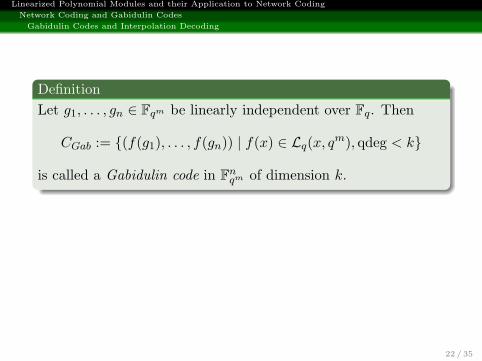
Let g1, . . . , gn ∈ Fqm be linearly independent over Fq. Then
CGab := {(f(g1), . . . , f(gn)) | f(x) ∈ Lq(x, qm), qdeg < k}
is called a Gabidulin code in Fnqm of dimension k.
Theorem
A Gabidulin code C ⊆ Fnqm of dimension k has minimum rank
distance n− k + 1, which is optimal (Singleton bound).Therefore, it is called a maximum rank distance (MRD) code.
22 / 35

Linearized Polynomial Modules and their Application to Network Coding
Network Coding and Gabidulin Codes
Gabidulin Codes and Interpolation Decoding
Definition
Let g1, . . . , gn ∈ Fqm be linearly independent over Fq. Then
CGab := {(f(g1), . . . , f(gn)) | f(x) ∈ Lq(x, qm), qdeg < k}
is called a Gabidulin code in Fnqm of dimension k.
Theorem
A Gabidulin code C ⊆ Fnqm of dimension k has minimum rank
distance n− k + 1, which is optimal (Singleton bound).Therefore, it is called a maximum rank distance (MRD) code.
22 / 35

Linearized Polynomial Modules and their Application to Network Coding
Network Coding and Gabidulin Codes
Gabidulin Codes and Interpolation Decoding
Example:Consider F22
∼= F2[α], with α2 + α+ 1 = 0. Fix g1 = 1, g2 = α(linearly independent). The Gabidulin code of length n = 2,dimension k = 1 and minimum distance n− k + 1 = 2 is
(0 0) 7→(
0 00 0
)f(x) = 0
(1 α) 7→(
1 00 1
)f(x) = x
(α α+ 1) 7→(
0 11 1
)f(x) = αx
(α+ 1 1) 7→(
1 11 0
)f(x) = (α+ 1)x
23 / 35
Linearized Polynomial Modules and their Application to Network Coding
Network Coding and Gabidulin Codes
Gabidulin Codes and Interpolation Decoding
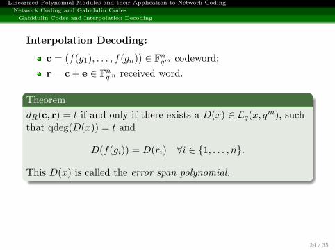
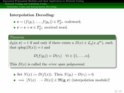
Interpolation Decoding:
c = (f(g1), . . . , f(gn)) ∈ Fnqm codeword;
r = c+ e ∈ Fnqm received word.
Theorem
dR(c, r) = t if and only if there exists a D(x) ∈ Lq(x, qm), such
that qdeg(D(x)) = t and
D(f(gi)) = D(ri) ∀i ∈ {1, . . . , n}.
This D(x) is called the error span polynomial.
Set N(x) := D(f(x)). Then N(gi)−D(ri) = 0.
=⇒ [N(x) −D(x)] ∈ M(g, r) (interpolation module)!
24 / 35
Linearized Polynomial Modules and their Application to Network Coding
Network Coding and Gabidulin Codes
Gabidulin Codes and Interpolation Decoding
Interpolation Decoding:
c = (f(g1), . . . , f(gn)) ∈ Fnqm codeword;
r = c+ e ∈ Fnqm received word.
Theorem
dR(c, r) = t if and only if there exists a D(x) ∈ Lq(x, qm), such
that qdeg(D(x)) = t and
D(f(gi)) = D(ri) ∀i ∈ {1, . . . , n}.
This D(x) is called the error span polynomial.
Set N(x) := D(f(x)). Then N(gi)−D(ri) = 0.
=⇒ [N(x) −D(x)] ∈ M(g, r) (interpolation module)!
24 / 35

Linearized Polynomial Modules and their Application to Network Coding
Network Coding and Gabidulin Codes
Gabidulin Codes and Interpolation Decoding
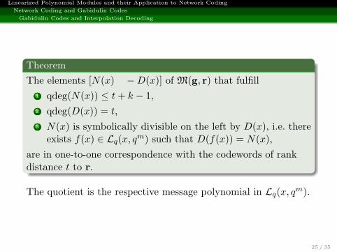
Theorem
The elements [N(x) −D(x)] of M(g, r) that fulfill
1 qdeg(N(x)) ≤ t+ k − 1,
2 qdeg(D(x)) = t,
3 N(x) is symbolically divisible on the left by D(x), i.e. thereexists f(x) ∈ Lq(x, q
m) such that D(f(x)) = N(x),
are in one-to-one correspondence with the codewords of rankdistance t to r.
The quotient is the respective message polynomial in Lq(x, qm).
25 / 35
Linearized Polynomial Modules and their Application to Network Coding
Network Coding and Gabidulin Codes
Gabidulin Codes and Interpolation Decoding
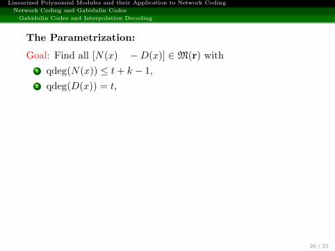
The Parametrization:
Goal: Find all [N(x) −D(x)] ∈ M(r) with
1 qdeg(N(x)) ≤ t+ k − 1,
2 qdeg(D(x)) = t,
Solution: If {b1, b2} is minimal basis (ordered by leadingpositions) with ℓ1, ℓ2 the respective weighted row q-degrees, then
λ(x) ◦ b1 + µ(x) ◦ b2 with
1 qdeg(λ(x)) ≤ t− ℓ1 + k − 1,
2 qdeg(µ(x)) = t− ℓ2 + k − 1 and µ(x) is monic
yield all the desired elements.
Proof: Based on the Predictable Leading Monomial Property.
26 / 35

Linearized Polynomial Modules and their Application to Network Coding
Network Coding and Gabidulin Codes
Gabidulin Codes and Interpolation Decoding
The Parametrization:
Goal: Find all [N(x) −D(x)] ∈ M(r) with
1 qdeg(N(x)) ≤ t+ k − 1,
2 qdeg(D(x)) = t,
Solution: If {b1, b2} is minimal basis (ordered by leadingpositions) with ℓ1, ℓ2 the respective weighted row q-degrees, then
λ(x) ◦ b1 + µ(x) ◦ b2 with
1 qdeg(λ(x)) ≤ t− ℓ1 + k − 1,
2 qdeg(µ(x)) = t− ℓ2 + k − 1 and µ(x) is monic
yield all the desired elements.
Proof: Based on the Predictable Leading Monomial Property.
26 / 35
Linearized Polynomial Modules and their Application to Network Coding
Network Coding and Gabidulin Codes
Gabidulin Codes and Interpolation Decoding
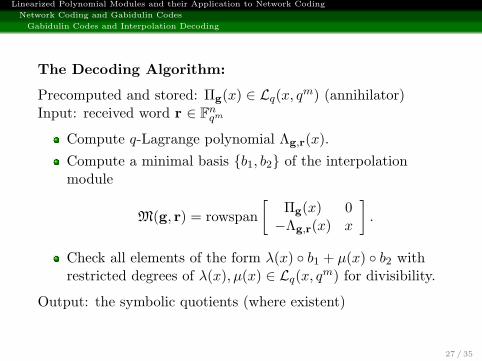
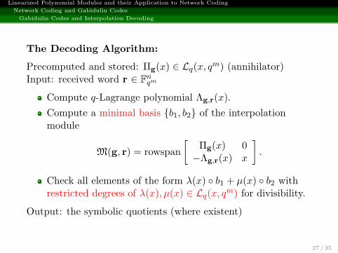
The Decoding Algorithm:
Precomputed and stored: Πg(x) ∈ Lq(x, qm) (annihilator)
Input: received word r ∈ Fnqm
Compute q-Lagrange polynomial Λg,r(x).
Compute a minimal basis {b1, b2} of the interpolationmodule
M(g, r) = rowspan
[Πg(x) 0
−Λg,r(x) x
].
Check all elements of the form λ(x) ◦ b1 + µ(x) ◦ b2 withrestricted degrees of λ(x), µ(x) ∈ Lq(x, q
m) for divisibility.
Output: the symbolic quotients (where existent)
27 / 35
Linearized Polynomial Modules and their Application to Network Coding
Network Coding and Gabidulin Codes
Gabidulin Codes and Interpolation Decoding
The Decoding Algorithm:
Precomputed and stored: Πg(x) ∈ Lq(x, qm) (annihilator)
Input: received word r ∈ Fnqm
Compute q-Lagrange polynomial Λg,r(x).
Compute a minimal basis {b1, b2} of the interpolationmodule
M(g, r) = rowspan
[Πg(x) 0
−Λg,r(x) x
].
Check all elements of the form λ(x) ◦ b1 + µ(x) ◦ b2 withrestricted degrees of λ(x), µ(x) ∈ Lq(x, q
m) for divisibility.
Output: the symbolic quotients (where existent)
27 / 35

Linearized Polynomial Modules and their Application to Network Coding
Network Coding and Gabidulin Codes
Gabidulin Codes and Interpolation Decoding
Example:Consider the Gabidulin code C over F23
∼= F2[α] (withα3 = α+ 1) with generator matrix
G =
(1 α α2
1 α2 α4
).
=⇒ dR = n− k + 1 = 3− 2 + 1 = 2=⇒ C is no-error correcting
Received word:r = ( α+ 1 0 α ).
Interpolation module:
M(r) = rowspan
[Πg(x) 0Λg,r(x) x
]= rowspan
[x8 + x 0
α2x4 + α5x x
].
28 / 35

Linearized Polynomial Modules and their Application to Network Coding
Network Coding and Gabidulin Codes
Gabidulin Codes and Interpolation Decoding
Example:Consider the Gabidulin code C over F23
∼= F2[α] (withα3 = α+ 1) with generator matrix
G =
(1 α α2
1 α2 α4
).
=⇒ dR = n− k + 1 = 3− 2 + 1 = 2=⇒ C is no-error correctingReceived word:
r = ( α+ 1 0 α ).
Interpolation module:
M(r) = rowspan
[Πg(x) 0Λg,r(x) x
]= rowspan
[x8 + x 0
α2x4 + α5x x
].
28 / 35
Linearized Polynomial Modules and their Application to Network Coding
Network Coding and Gabidulin Codes
Gabidulin Codes and Interpolation Decoding
Finding the minimal basis with the Euclidean algorithm:
x8 + x = (α3x2) ◦ (α2x4 + α5x) + (α6x2 + x).
Since qdeg(α3x2) + k − 1 = 2 ≥ 1 = qdeg(α6x2 + x), thealgorithm terminates and a minimal basis (w.r.t. the(0, 1)-weighted 2-degree) of this module is[
0 xx α3x2
]◦[
x8 + x 0α2x4 + α5x x
]︸ ︷︷ ︸
original basis
=
[α2x4 + α5x xα6x2 + x α3x2
]︸ ︷︷ ︸
minimal basis
.
29 / 35

Linearized Polynomial Modules and their Application to Network Coding
Network Coding and Gabidulin Codes
Gabidulin Codes and Interpolation Decoding
Parametrization λ(x) ◦ b1 + µ(x) ◦ b2:
Use all λ(x) ∈ L2(x, 23) with 2-degree 0 and all monic
µ(x) ∈ L2(x, 23) with 2-degree 0.
=⇒ λ(x) = a0x, a0 ∈ F23 , and µ(x) = x
E.g. for a0 = α:
(αx) ◦ [α2x4 + α5x x] + [α6x2 + x α3x2]
= [α3x4 + α6x αx] + [α6x2 + x α3x2]
= [α3x4 + α6x2 + α2x α3x2 + αx]
Symbolic division:
α3x4 + α6x2 + α2x = (α3x2 + αx) ◦ ( x2 + αx︸ ︷︷ ︸message polynomial
)
30 / 35
Linearized Polynomial Modules and their Application to Network Coding
Network Coding and Gabidulin Codes
Gabidulin Codes and Interpolation Decoding
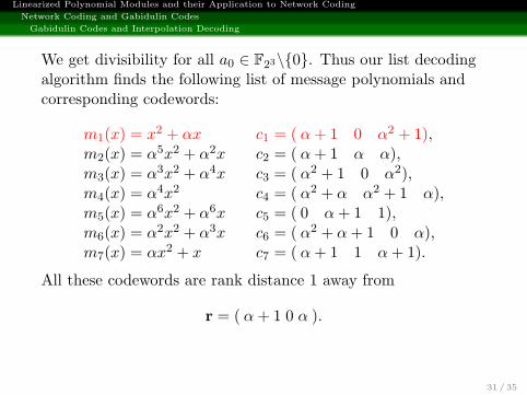
We get divisibility for all a0 ∈ F23\{0}. Thus our list decodingalgorithm finds the following list of message polynomials andcorresponding codewords:
m1(x) = x2 + αx c1 = ( α+ 1 0 α2 + 1),m2(x) = α5x2 + α2x c2 = ( α+ 1 α α),m3(x) = α3x2 + α4x c3 = ( α2 + 1 0 α2),m4(x) = α4x2 c4 = ( α2 + α α2 + 1 α),m5(x) = α6x2 + α6x c5 = ( 0 α+ 1 1),m6(x) = α2x2 + α3x c6 = ( α2 + α+ 1 0 α),m7(x) = αx2 + x c7 = ( α+ 1 1 α+ 1).
All these codewords are rank distance 1 away from
r = ( α+ 1 0 α ).
Note: Hamming distance can be 1, 2 or 3.
31 / 35

Linearized Polynomial Modules and their Application to Network Coding
Network Coding and Gabidulin Codes
Gabidulin Codes and Interpolation Decoding
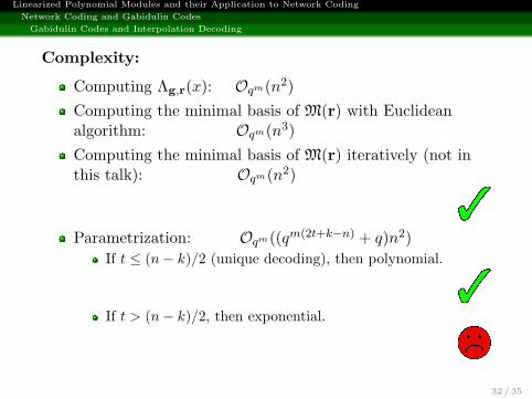
Complexity:
Computing Λg,r(x): Oqm(n2)
Computing the minimal basis of M(r) with Euclideanalgorithm: Oqm(n
3)
Computing the minimal basis of M(r) iteratively (not inthis talk): Oqm(n
2)
Parametrization: Oqm((qm(2t+k−n) + q)n2)
If t ≤ (n− k)/2 (unique decoding), then polynomial.
If t > (n− k)/2, then exponential.
32 / 35
Linearized Polynomial Modules and their Application to Network Coding
Network Coding and Gabidulin Codes
Gabidulin Codes and Interpolation Decoding
Complexity:
Computing Λg,r(x): Oqm(n2)
Computing the minimal basis of M(r) with Euclideanalgorithm: Oqm(n
3)
Computing the minimal basis of M(r) iteratively (not inthis talk): Oqm(n
2)
Parametrization: Oqm((qm(2t+k−n) + q)n2)
If t ≤ (n− k)/2 (unique decoding), then polynomial.
If t > (n− k)/2, then exponential.
32 / 35

Linearized Polynomial Modules and their Application to Network Coding
Network Coding and Gabidulin Codes
Gabidulin Codes and Interpolation Decoding
Idea to improve parametrization (open problem):
When finding all [N(x) −D(x)] ∈ M(r) with the degreerestrictions we can impose extra condition that the errorspan polynomial D(x) has only distinct roots.
Open problem: How to parametrize this condition?
In Reed-Solomon case it can be done with a curve fittingalgorithm (based on Wu’s algorithm). This idea does notwork in the linearized case.
33 / 35

Linearized Polynomial Modules and their Application to Network Coding
Summary and Conclusion
1 Linearized PolynomialsThe Ring Lq(x, q
m)Modules over Lq(x, q
m)
2 Network Coding and Gabidulin CodesIntroductionGabidulin Codes and Interpolation Decoding
3 Summary and Conclusion
Linearized Polynomial Modules and their Application to Network Coding
Summary and Conclusion
Summary and Conclusion
Lq(x, qm) is non-commutative ring with Euclidean
algorithm
Lq(x, qm)ℓ, as left module, can be equipped with monomial
order (e.g. (k, . . . , kℓ)-weighted TOP order)
Minimal basis = basis with all distinct leading positions
Predictable Leading Monomial Property holds for minimalbases
PLMP gives rise to parametrizations
Remark: Linearized polynomials are skew polynomials, manystatements can be proven in this setting, as well.
34 / 35

Linearized Polynomial Modules and their Application to Network Coding
Summary and Conclusion
Decoding in the network coding setting (Gabidulin codes)can be translated to a parametrization in the interpolationmodule.Set up algebraic decoding algorithm, that finds allcodewords within the ball of radius t around a givenreceived word, for any decoding radius t.Can easily be altered to find all closest codewords to agiven received word.Complexity is exponential in code length iff the decodingradius is beyond the unique decoding radius.Nonetheless, it is still feasible for radii close to the uniquedecoding radius.
Thank you for your attention!
35 / 35