Linear Regression- An 80 Year study of the Dow Jones

Industrial AverageTehya Singleton

Rivers AP Statistics

Chart Copied From Fathom

Year Since 1930 Dow Price Predicted Dow Price Residuals Transformation Dow Price Transformation Prediction Transformation Residuals ln since 1930 ln dow price

1930 0 233.99 -2435.42 -2669.41 2.3692 1.87328 0.495915 #Domain error# 5.45528

1931 1 135.39 -2310.12 -2445.51 2.13159 1.90036 0.231231 0 4.90816

1932 2 53.89 -2184.83 -2238.72 1.73151 1.92743 -0.195921 0.693147 3.98694

1933 3 90.77 -2059.54 -2150.31 1.95794 1.9545 0.00343931 1.09861 4.50833

1934 4 88.05 -1934.24 -2022.29 1.94473 1.98158 -0.0368473 1.38629 4.4779

1935 5 126.23 -1808.95 -1935.18 2.10116 2.00865 0.0925124 1.60944 4.83811

1936 6 164.86 -1683.65 -1848.51 2.21712 2.03572 0.181392 1.79176 5.1051

1937 7 184.01 -1558.36 -1742.37 2.26484 2.0628 0.202044 1.94591 5.21499

1938 8 141.2 -1433.06 -1574.26 2.14983 2.08987 0.0599637 2.07944 4.95018

1939 9 143.26 -1307.77 -1451.03 2.15612 2.11694 0.0391804 2.19722 4.96466

1940 10 126.14 -1182.47 -1308.61 2.10085 2.14402 -0.0431653 2.30259 4.83739

1941 11 128.79 -1057.18 -1185.97 2.10988 2.17109 -0.0612096 2.3979 4.85818

1942 12 105.72 -931.884 -1037.6 2.02416 2.19817 -0.174008 2.48491 4.66079

1943 13 137.25 -806.59 -943.84 2.13751 2.22524 -0.0877265 2.56495 4.9218

1944 14 146.11 -681.295 -827.405 2.16468 2.25231 -0.0876325 2.63906 4.98436

1945 15 162.88 -556.001 -718.881 2.21187 2.27939 -0.0675183 2.70805 5.09301

1946 16 201.56 -430.706 -632.266 2.3044 2.30646 -0.00205528 2.77259 5.30609

1947 17 183.18 -305.412 -488.592 2.26288 2.33353 -0.0706552 2.83321 5.21047

1948 18 181.33 -180.117 -361.447 2.25847 2.36061 -0.102137 2.89037 5.20032

1949 19 175.92 -54.8228 -230.743 2.24532 2.38768 -0.142365 2.94444 5.17003

1950 20 209.4 70.4717 -138.928 2.32098 2.41475 -0.0937773 2.99573 5.34425

1951 21 257.86 195.766 -62.0938 2.41138 2.44183 -0.0304436 3.04452 5.55242

1952 22 279.56 321.061 41.5008 2.44648 2.4689 -0.0224261 3.09104 5.63322

1953 23 275.38 446.355 170.975 2.43993 2.49597 -0.0560423 3.13549 5.61815

1954 24 347.92 571.65 223.73 2.54148 2.52305 0.0184311 3.17805 5.85197

1955 25 465.85 696.944 231.094 2.66825 2.55012 0.118124 3.21888 6.14386

1956 26 517.81 822.239 304.429 2.71417 2.5772 0.136975 3.2581 6.24961

1957 27 508.52 947.533 439.013 2.70631 2.60427 0.102039 3.29584 6.2315

1958 28 502.99 1072.83 569.838 2.70156 2.63134 0.0702167 3.3322 6.22057

1959 29 674.88 1198.12 523.242 2.82923 2.65842 0.17081 3.3673 6.51453

1960 30 616.73 1323.42 706.687 2.7901 2.68549 0.104605 3.4012 6.42443

1961 31 705.37 1448.71 743.341 2.84842 2.71256 0.135854 3.43399 6.55872

1962 32 597.93 1574.01 976.076 2.77665 2.73964 0.0370134 3.46574 6.39347

1963 33 695.43 1699.3 1003.87 2.84225 2.76671 0.0755429 3.49651 6.54453

1964 34 841.1 1824.6 983.495 2.92485 2.79378 0.131063 3.52636 6.73471

1965 35 881.74 1949.89 1068.15 2.94534 2.82086 0.124483 3.55535 6.7819

1966 36 847.38 2075.18 1227.8 2.92808 2.84793 0.0801469 3.58352 6.74215

1967 37 904.24 2200.48 1296.24 2.95628 2.875 0.0812788 3.61092 6.80709

1968 38 883 2325.77 1442.77 2.94596 2.90208 0.0438822 3.63759 6.78333

1969 39 815.47 2451.07 1635.6 2.91141 2.92915 -0.0177441 3.66356 6.70376

1970 40 734.12 2576.36 1842.24 2.86577 2.95623 -0.0904586 3.68888 6.59867

1971 41 858.43 2701.66 1843.23 2.9337 2.9833 -0.0495944 3.71357 6.75511

1972 42 924.74 2826.95 1902.21 2.96602 3.01037 -0.0443532 3.73767 6.82951

1973 43 926.4 2952.25 2025.85 2.9668 3.03745 -0.0706479 3.7612 6.83131

1974 44 757.43 3077.54 2320.11 2.87934 3.06452 -0.185177 3.78419 6.62993

1975 45 831.51 3202.83 2371.32 2.91987 3.09159 -0.171726 3.80666 6.72324

1976 46 984.64 3328.13 2343.49 2.99328 3.11867 -0.12539 3.82864 6.89228

1977 47 890.07 3453.42 2563.35 2.94942 3.14574 -0.196317 3.85015 6.7913

1978 48 862.27 3578.72 2716.45 2.93564 3.17281 -0.237171 3.8712 6.75957

1979 49 846.42 3704.01 2857.59 2.92759 3.19989 -0.272302 3.89182 6.74102

1980 50 935.32 3829.31 2893.99 2.97096 3.22696 -0.256001 3.91202 6.84089

1981 51 952.34 3954.6 3002.26 2.97879 3.25404 -0.275243 3.93183 6.85892

1982 52 808.6 4079.9 3271.3 2.90773 3.28111 -0.373375 3.95124 6.6953

1983 53 1199.22 4205.19 3005.97 3.0789 3.30818 -0.229283 3.97029 7.08943

1984 54 1115.28 4330.49 3215.21 3.04738 3.33526 -0.287872 3.98898 7.01686

1985 55 1347.45 4455.78 3108.33 3.12951 3.36233 -0.232817 4.00733 7.20597

1986 56 1775.31 4581.07 2805.76 3.24927 3.3894 -0.140129 4.02535 7.48173

1987 57 2572.07 4706.37 2134.3 3.41028 3.41648 -0.00619381 4.04305 7.85247

1988 58 2128.73 4831.66 2702.93 3.32812 3.44355 -0.11543 4.06044 7.66328

1989 59 2660.66 4956.96 2296.3 3.42499 3.47062 -0.0456344 4.07754 7.88633

1990 60 2905.2 5082.25 2177.05 3.46318 3.4977 -0.0345213 4.09434 7.97426

1991 61 3024.82 5207.55 2182.73 3.4807 3.52477 -0.0440714 4.11087 8.01461

1992 62 3393.78 5332.84 1939.06 3.53068 3.55184 -0.0211608 4.12713 8.1297

1993 63 3539.47 5458.14 1918.67 3.54894 3.57892 -0.0299799 4.14313 8.17173

1994 64 3764.5 5583.43 1818.93 3.57571 3.60599 -0.0302844 4.15888 8.23337

1995 65 4708.47 5708.73 1000.26 3.67288 3.63307 0.0398145 4.17439 8.45712

1996 66 5528.91 5834.02 305.11 3.74264 3.66014 0.0825007 4.18965 8.61775

1997 67 8222.61 5959.31 -2263.3 3.91501 3.68721 0.227797 4.20469 9.01464

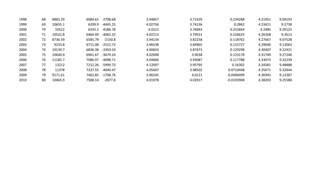
1998 68 8883.29 6084.61 -2798.68 3.94857 3.71429 0.234288 4.21951 9.09193

1999 69 10655.1 6209.9 -4445.25 4.02756 3.74136 0.2862 4.23411 9.2738

2000 70 10522 6335.2 -4186.78 4.0221 3.76843 0.253664 4.2485 9.26122

2001 71 10522.8 6460.49 -4062.32 4.02213 3.79551 0.226625 4.26268 9.2613

2002 72 8736.59 6585.79 -2150.8 3.94134 3.82258 0.118762 4.27667 9.07528

2003 73 9233.8 6711.08 -2522.72 3.96538 3.84965 0.115727 4.29046 9.13063

2004 74 10139.7 6836.38 -3303.33 4.00603 3.87673 0.129298 4.30407 9.22421

2005 75 10640.9 6961.67 -3679.24 4.02698 3.9038 0.123178 4.31749 9.27246

2006 76 11185.7 7086.97 -4098.71 4.04866 3.93087 0.117788 4.33073 9.32239

2007 77 13212 7212.26 -5999.73 4.12097 3.95795 0.16302 4.34381 9.48888

2008 78 11378 7337.55 -4040.47 4.05607 3.98502 0.0710448 4.35671 9.33944

2009 79 9171.61 7462.85 -1708.76 3.96245 4.0121 -0.0496499 4.36945 9.12387

2010 80 10465.9 7588.14 -2877.8 4.01978 4.03917 -0.0193908 4.38203 9.25588

Graphs and Questions

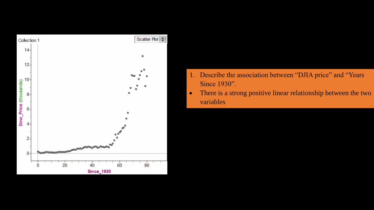
1. Describe the association between “DJIA price” and “Years

Since 1930”.

There is a strong positive linear relationship between the two

variables

2. What is the equation for your linear model? (Use

descriptive variables)

Dow price=125.3(since 1930)-2.4425

3. Interpret the slope of the line in context.

As the “years since” increases the “Dow Price” also

increases.

4. Does the y-intercept of your model have a meaningful

interpretation or is it just a hypothetical base value?

Explain.

The y-intercept is the Dow price over 80 years. It is a

meaningful interpretation these are numbers from the

stock market there is always a meaning behind those

numbers.

5. Look at the residuals plot for your linear

model. Do you have any concerns about

predictions made by your

model? Explain.

No, the residual plot looks exactly like

the linear model the only difference is the

direction they are facing.

6. What is the equation of your new model? (Use descriptive

variables)

Transformation Dow price=0.02707(since 1930)-50.38

7. Interpret the slope of the line in context.

• As the “years since” increases the “Dow Price” also

increases.

8. This time, does the y-intercept of your model have a meaningful

interpretation? Explain.

• Yes it’s the same data it’s just a transformation of the data

9. The residuals plot for your

transformed model still doesn’t look

perfect, but has it improved? How

do you feel about the

appropriateness of your new

model?

• It has improved. Its looks like the

linear model so it’s appropriate to

use.

Collection 1

Transformation_Dow_Price

Year 0.972085

S1 = correlation

10. What is the correlation for your transformed data? What does this indicate about the

association?

The correlation is 0.97 there is a strong positive association

11. What is R2 for your transformed data? Interpret this value in context.

R2 is 0.94 and that tells us that 94% of the variation in y is explained by the variation in x

12. Use your model to make a prediction about the Dow price in July of 2012.

The predicted Dow price for July 2012 is 252101.1575

13. You will most likely retire sometime between 2040 and 2050. What does your model predict

for the Dow price in 2045? Comment on the appropriateness of this prediction.

• The predicted Dow price for 2045 is 256236.0575 that prediction is fairly appropriate based on

the fact that as the years go by the predicted Dow price increases.

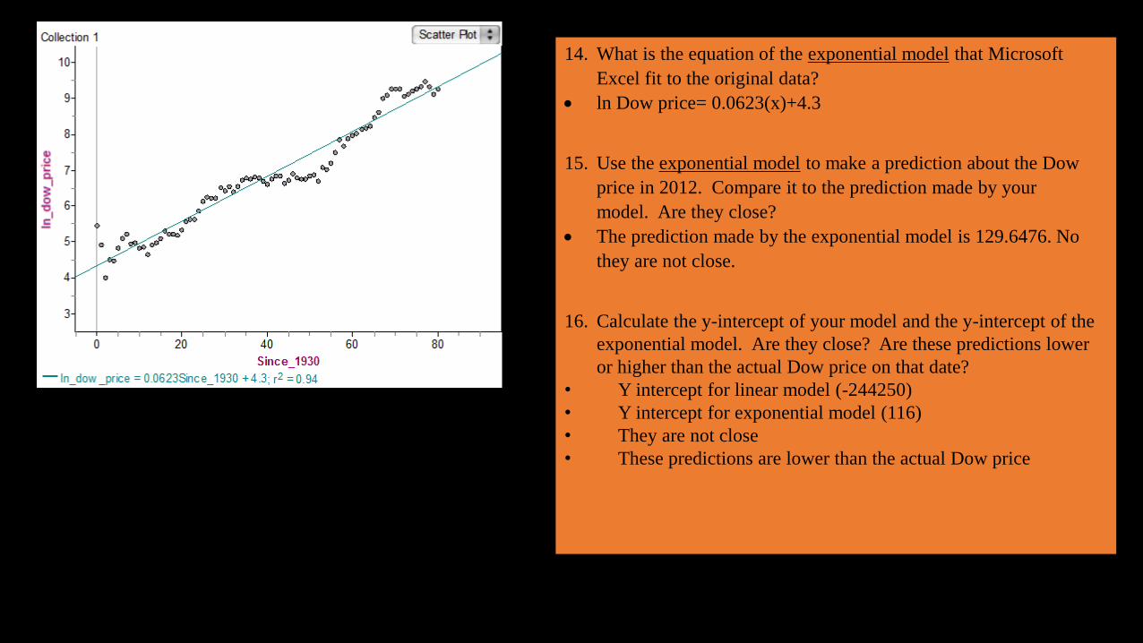
14. What is the equation of the exponential model that Microsoft

Excel fit to the original data?

ln Dow price= 0.0623(x)+4.3

15. Use the exponential model to make a prediction about the Dow

price in 2012. Compare it to the prediction made by your

model. Are they close?

The prediction made by the exponential model is 129.6476. No

they are not close.

16. Calculate the y-intercept of your model and the y-intercept of the

exponential model. Are they close? Are these predictions lower

or higher than the actual Dow price on that date?

• Y intercept for linear model (-244250)

• Y intercept for exponential model (116)

• They are not close

• These predictions are lower than the actual Dow price

17. Recently, concerns about the U.S. economy, unemployment

rate, national debt, foreign relations, the world economy,

financial troubles in countries like Greece and China, climate

change, and population expansion, among others have led

many to question whether common stocks will continue to

grow at 10-12% as we move into the future. Soon, you will

have finished college, secured a position in a fulfilling

career, and started earning a rewarding salary. You, too, will

have to make decisions about the best way to invest your

hard earned money in order to insure that you have a healthy

nest egg to retire on. You’ve just studied the trend of the

broader market over an 80-year period that included

numerous wars, periods of political unrest, economic

recessions, energy crises, population shifts, and corporate

scandals (just to name a few). So, are you convinced? How

do you feel about the strength of this trend? Will the market

continue to reward you the way it rewarded long-term

investors of the previous century? Or, will these new

troubling developments send you seeking other methods of

investment? Explain.

I am convinced. Even with the new troubling developments I feel that there will still be a strong trend in the future because this isn’t the first time that there has been problems facing the economy. The market is never down for to long and I am confident that it will continue to reward myself and future investors like it has for the previous.

Linear

Exponential

Power

The exponential graph best fits the data gathered in this study.