LINEAR PROGRAMMING PROBLEMS FOR …math.ucdenver.edu/graduate/thesis/Thipwiwatpotjana_PhDThesis.pdfThipwiwatpotjana, Phantipa (Ph.D., Applied Mathematics) Linear Programming Problems

LINEAR PROGRAMMING PROBLEMS FOR GENERALIZED

UNCERTAINTY

by

Phantipa Thipwiwatpotjana

M.S., Clemson University, South Carolina, USA, 2004

B.S., Chiang Mai University, Chiang Mai, Thailand, 1999

A thesis submitted to the

University of Colorado Denver

in partial fulfillment

of the requirements for the degree of

Doctor of Philosophy

Mathematical and Statistical Sciences

2010

This thesis for the Doctor of Philosophy

degree by

Phantipa Thipwiwatpotjana

has been approved

by

Weldon Lodwick

Stephen Billups

George Corliss

Alexander Engau

Burt Simon

Date

Thipwiwatpotjana, Phantipa (Ph.D., Applied Mathematics)

Linear Programming Problems for Generalized Uncertainty

Thesis directed by Professor Weldon Lodwick

ABSTRACT

Uncertainty occurs when there is more than one realization that can repre-

sent an information. This dissertation concerns merely discrete realizations of an

uncertainty. Different interpretations of an uncertainty and their relationships

are addressed when the uncertainty is not a probability of each realization. A

well known model that can handle a linear programming problem with proba-

bility uncertainty is an expected recourse model. If uncertainties in the problem

have possibility interpretations, an expected average model, which is comparable

to an expected recourse model, will be used. These two models can be mixed

when we have both probability and possibility uncertainties in the problem,

provided these uncertainties do not occur in the same constraint.

This dissertation develops three new solution methods for a linear optimiza-

tion problem with generalized uncertainty. These solutions are a pessimistic, an

optimistic, and a minimax regret solution. The interpretations of uncertainty

in a linear programming problem with generalized uncertainty are not limited

to probability and possibility. They can be also necessity, plausibility, belief,

random set, probability interval, probability on sets, cloud, and interval-valued

probability measure. These new approaches can handle more than one interpre-

tation of uncertainty in the same constraint, which has not been done before.

Lastly, some examples and realistic application problems are presented to illus-

trate these new approaches. Some comparisons between these solutions and a

solution from the mixed expected average and expected recourse model when

uncertainties are probability and possibility are mentioned.

This abstract accurately represents the content of the candidate’s thesis. I

recommend its publication.

SignedWeldon Lodwick

I dedicate this work to my parents,

Amporn and Wut.

ACKNOWLEDGMENT

I am most grateful to my adviser, Dr. Weldon A. Lodwick, who introduced

me to the uncertainty world, for his guidance, support, and commitment. His

invaluable advice, patience, and encouragement make this work possible.

I am thankful to Dr. Stephen Billups, Dr. George Corliss, Dr. Alexander

Engau, and Dr. Burt Simon for serving on my Ph.D. committee. I appreciate

their time, comments and suggestions that were very helpful in developing the

research. I express my special thanks for their corrections and suggestions that

improved this dissertation.

I would like to thank the Thai government officers who took care of me

while I am in the US. I extend my appreciation to the Bateman family and the

Department of Mathematical and Statistical Sciences, University of Colorado

at Denver, who provide the financial support throughout my study after the

support from the Thai government was terminated.

Finally, I am most thankful to my mother, Amporn, for her care, love, and

support. Warm thanks for my sister, Yui, and my brother, Yook, for sharing

their opinions. Special thanks to Iris for her kindness for a Thai girl. To, Tur,

for his love, care, support, and help. Because of their encouragement, support,

help, and love, my success is also theirs.

CONTENTS

Figures . . . . . . . . . . . . . . . . . . . . . . . . . . . . . . . . . . . . x

Tables . . . . . . . . . . . . . . . . . . . . . . . . . . . . . . . . . . . . . xi

Chapter

1. Introduction to the dissertation . . . . . . . . . . . . . . . . . . . . . 1

1.1 Problem statement . . . . . . . . . . . . . . . . . . . . . . . . . . . 4

1.2 Research direction and organization of the dissertation . . . . . . . 9

2. Some selected uncertainty interpretations . . . . . . . . . . . . . . . . 12

2.1 Possibility theory . . . . . . . . . . . . . . . . . . . . . . . . . . . . 13

2.2 Random sets . . . . . . . . . . . . . . . . . . . . . . . . . . . . . . 24

2.2.1 Upper and lower expected values generated by random sets . . . 39

2.2.2 The random set generated by an incomplete random set information 50

2.2.3 The random set generated by a possibility distribution or possibil-

ity of some subset of U . . . . . . . . . . . . . . . . . . . . . . . . 50

2.2.4 The random set generated by a necessity distribution or necessity

of some subset of U . . . . . . . . . . . . . . . . . . . . . . . . . 52

2.2.5 The random set generated by a belief distribution . . . . . . . . . 53

2.2.6 The random set generated by a plausibility distribution . . . . . . 53

2.3 Interval-valued probability measures (IVPMs) . . . . . . . . . . . . 54

2.3.1 Upper and lower expected values generated by IVPMs . . . . . . 66

2.4 Clouds . . . . . . . . . . . . . . . . . . . . . . . . . . . . . . . . . . 70

2.5 Relationships of some selected uncertainty interpretations . . . . . . 75

vii

3. Linear optimization under uncertainty: literature review . . . . . . . 80

3.1 Deterministic model . . . . . . . . . . . . . . . . . . . . . . . . . . 81

3.2 Stochastic models . . . . . . . . . . . . . . . . . . . . . . . . . . . . 83

3.2.1 Stochastic program with expected recourse . . . . . . . . . . . . . 85

3.3 Minimax regret model . . . . . . . . . . . . . . . . . . . . . . . . . 90

3.4 Possibility model . . . . . . . . . . . . . . . . . . . . . . . . . . . . 93

3.5 Mixed model of probability and possibility . . . . . . . . . . . . . . 99

3.6 Mixed uncertainties model . . . . . . . . . . . . . . . . . . . . . . . 101

4. Linear optimization under uncertainty: pessimistic, optimistic, and

minimax regret approaches . . . . . . . . . . . . . . . . . . . . . . . . 107

4.1 Pessimistic and optimistic expected recourse problems . . . . . . . 109

4.1.1 Pessimistic and optimistic expected recourse problems generated

by random sets with finite realizations . . . . . . . . . . . . . . . 115

4.1.2 Pessimistic and optimistic expected recourse problems generated

by IVPMs with finite realizations . . . . . . . . . . . . . . . . . . 121

4.2 Minimax regret of the expected recourse problems . . . . . . . . . . 123

4.2.1 A relaxation procedure for minimax regret of the expected recourse

problems . . . . . . . . . . . . . . . . . . . . . . . . . . . . . . . 125

4.3 Storage or selling costs in expected recourse problems . . . . . . . . 132

4.3.1 Selling costs in expected recourse problems . . . . . . . . . . . . . 133

4.3.2 Storage costs in expected recourse problems . . . . . . . . . . . . 134

4.4 Comparison between pessimistic, optimistic, minimax regret ap-

proaches and the reviewed approaches . . . . . . . . . . . . . . . . 135

5. Examples and applications . . . . . . . . . . . . . . . . . . . . . . . . 139

viii

5.1 Farming example . . . . . . . . . . . . . . . . . . . . . . . . . . . . 139

5.1.1 A random set version of the farming example . . . . . . . . . . . 143

5.2 An application for radiation shielding design of radiotherapy treat-

ment vaults . . . . . . . . . . . . . . . . . . . . . . . . . . . . . . . 149

6. Conclusion . . . . . . . . . . . . . . . . . . . . . . . . . . . . . . . . . 158

Appendix

A. How to obtain a basic probability assignment function m from a given

belief measure Bel . . . . . . . . . . . . . . . . . . . . . . . . . . . . 161

B. The nestedness requirement of focal elements for a possibility measure 163

References . . . . . . . . . . . . . . . . . . . . . . . . . . . . . . . . . . . 167

ix

FIGURES

Figure

1.1 Uncertainty interpretations: A −−→ B represents that an uncertainty

interpretation B contains information given by an uncertainty inter-

pretation A, and A −−→ B represents that A is a special case of

B. . . . . . . . . . . . . . . . . . . . . . . . . . . . . . . . . . . . . 10

2.1 Venn diagram of an opinion poll for a Colorado governor’s election. 18

2.2 Possibility measure defined on U = u1, u2, . . . , u7. . . . . . . . . . 22

2.3 A finite representation of an infinite random set. . . . . . . . . . . 33

2.4 A random set generated by possibility distribution. . . . . . . . . . 51

2.5 A cloud on R with an α-cut at α = 0.6. . . . . . . . . . . . . . . . 71

2.6 A cloud represents an IVPM. . . . . . . . . . . . . . . . . . . . . . 72

2.7 Uncertainty interpretations: A −−→ B : there is an uncertainty in-

terpretation B contains information given by an uncertainty inter-

pretation A, A −−→ B : A is a special case of B, A ←→ B : A and

B can be derived from each other, and A · · · → B : B generalized A. 77

3.1 Feasible region and the unique optimal solution of the production

scheduling problem (3.1). . . . . . . . . . . . . . . . . . . . . . . . 83

5.1 An example of a radiation room. . . . . . . . . . . . . . . . . . . . 150

x

TABLES

Table

2.1 Probability theory versus possibility theory: comparison of mathe-

matical properties for finite sets . . . . . . . . . . . . . . . . . . . . 23

2.2 The number of belief and plausibility terms required for finding two

density functions for the lowest and the highest expected values of θ

by using Theorem 2.17 versus by solving two LP problems. . . . . . 46

2.3 The differences between IVPMs and clouds . . . . . . . . . . . . . 72

3.1 Productivity information shows the output of products per unit of

raw materials, the unit costs of raw materials, the demand for the

products, and the limitation of the total amount of raw materials. . 82

3.2 Computational results for different models of the production plan-

ning problem. . . . . . . . . . . . . . . . . . . . . . . . . . . . . . . 105

4.1 Computational Results for the new approaches and the reviewed ap-

proach of the production planning problem. . . . . . . . . . . . . . 137

5.1 Data for farming problem. . . . . . . . . . . . . . . . . . . . . . . . 140

5.2 An optimal solution based on expected yields. . . . . . . . . . . . . 140

5.3 The scenarios of yields for all crops. . . . . . . . . . . . . . . . . . . 141

5.4 An optimal solution based on the expected recourse problem (5.2). 142

5.5 Optimal solutions based on the pessimistic and optimistic expected

recourse of the farming problem. P = pessimistic, O = optimistic,

R = minimax regret. . . . . . . . . . . . . . . . . . . . . . . . . . . 147

xi

5.6 A pessimistic, an optimistic, a minimax regret, and an extreme sce-

nario solution for the radiation shielding design problem. . . . . . . 157

xii

1. Introduction to the dissertation

This dissertation develops a technique for solving linear optimizations un-

der uncertainty problems that have discrete realizations for broad classes of

uncertainty not studied and analyzed before. We study optimization under un-

certainty in which the probability density mass value of each realization is not

known with certainty. Information attached to an uncertainty can be categorized

into different interpretations. The interpretations of uncertainty information as-

sociated with this thesis are probability, belief, plausibility, necessity, possibility,

random set, probability interval, probability on sets, cloud, and interval-valued

probability measure (IVPM). For convenience, we call these interpretations of

uncertainty ‘PC-BRIN ’. We develop an approach to compute a pessimistic, an

optimistic, and a robust (minimum of maximum regret) solution for a linear

programming (LP) problem with these uncertainty interpretations. These prob-

lems are solved based on the transformation of a linear optimization problem

with uncertainty to a set of expected recourse models.

An expected recourse model is a paradigm to solve a stochastic program-

ming problem. Stochastic programming is the study of practical procedures for

decision making under uncertainty over time. Stochastic programs are mathe-

matical programs (linear, integer, mixed-integer, nonlinear) where some of the

data incorporated into the objective or constraints are uncertain with a proba-

bility interpretation. An expected recourse model requires that one makes one

decision now and minimizes the expected costs (or evaluations) of the conse-

1

quences of that decision. We consider a two stage expected recourse model in

this thesis. The first stage is as a decision that one needs to make now, and the

second stage is as a decision based on what has happened. The objective is to

minimize the expected costs of all decisions taken.

We refer to a probability interpretation of uncertainty when we can create

or assume a probability for each realization from an experiment without using

any prior knowledge. For example, we will not assume that a coin is fair when

we know nothing about this coin. The other interpretations of an uncertainty

information mentioned above (except probability) share the same behavior, i.e.,

the information that leads to one of those interpretations is not enough to obtain

a probability for each realization. Instead, an appropriate function is created

based on information provided.

Let U be a finite set of all realizations of an uncertainty u. A belief in-

terpretation of uncertainty is given in the form of a belief function, Bel, which

maps from an event (a subset of U) to a number between 0 and 1. For an event

A, Bel(A) can be interpreted as one’s degree of belief that the truth of u lies

in A. The probability may or may not coincide with the degree of belief about

an event of u. If we know the probabilities of events, then we will surely adopt

them as the degrees of belief. But, if we do not know the probabilities, then it

will be an extraordinary coincidence for the degrees of belief to be equal to their

probability. In general, sum of the probability of two mutually disjoint events

is equal to the probability of the union of those two events. This statement is

relaxed when the function is a belief function. Intuitively, one’s degree of belief

that the truth lies in A1 plus the degree of belief that the truth lies in A2 is

2

always less than or equal to the degree of belief that the truth lies in A1 ∪ A2.

G. Shafer, [60], mentioned that one’s beliefs that the truth of u lies in an

event A are not fully described by one’s degree of belief Bel(A). One may

also have some doubts about A. The degree of doubt can be expressed in the

form Dou(A) = Bel(Ac). A plausibility interpretation of uncertainty is closely

related to a belief because a plausibility function, Pl, can be derived from a

belief function, and vice versa, by using Pl(A) = 1− Bel(Ac). One’s degree of

plausibility Pl(A) expresses that one fails to doubt A or one finds A plausible.

Hence, Bel and Pl convey the same information, as we shall see in many ex-

amples throughout the thesis. A necessity and a possibility interpretations of

uncertainty are special versions of belief and plausibility, respectively. We call

belief and plausibility functions necessity and possibility functions, Nec and

Pos, when for events A1 and A2, Bel(A1 ∩ A2) = min [Bel(A1), Bel(A2)] and

Pl(A1∪A2) = max [Pl(A1), P l(A2)], respectively. The mathematical definitions

and some properties of belief, plausibility, necessity and possibility functions are

provided in Section 2.1.

An uncertainty provided in a form of random set interpretation has informa-

tion as a set of probabilities that are bounded above and below by plausibilities

and beliefs. A probability interval is an interval mapping from each element of U

to its corresponding interval [a, a], where [a, a] ⊆ [0, 1]. An IVPM interpretation

of uncertainty has information as intervals on probability of A, for every subset

A of U . A cloud is defined differently from IVPM. However, it turns out that

a cloud is an example of IVPM. More details on random set, cloud, and IVPM

interpretations are in Chapter 2. Probability on sets is a partial information of

3

probability, i.e., we know a value of P (A) for some A ⊆ U , but it is not enough

to obtain the probability of each realization in U . Probability intervals and

probability on sets can be viewed as examples of IVPM. Thus, the uncertainty

interpretations over finite realizations we include in our analysis are: probabil-

ity, belief, plausibility, necessity, possibility, random set, probability interval,

probability on sets, cloud, and IVPM, or PC-BRIN, in short.

1.1 Problem statement

The problem which is the focus of this thesis is

minx

c Tx s.t. Ax ≥ b, Bx ≥ d, x ≥ 0. (1.1)

We sometimes call (1.1) an LP problem with (generalized or mixed) uncertainty.

This dissertation tries to answer the question of how to solve (1.1). To date, the

theory and solution methods for (1.1) have not been developed when A, b, and

c have only one of the PC-BRIN uncertainty interpretations, except probability

and possibility. Moreover, when A, b, and c are mixtures of all the PC-BRIN

uncertainty interpretations within one constraint, there is no theory or solution

method yet to deal with this case. The significance of what is presented is

that problems possessing these uncertainty interpretations can be modeled and

solved directly from their true, basic, uncertainties. That is, the model is more

faithful to its underlying properties. Secondly, the model is faithful to the data

available.

We provide a simple LP problem with uncertainty without solving it for the

purpose of showing that uncertainty information, which does not have proba-

bility interpretation, may be an integral part of in an LP model. Suppose that

4

a tour guide wants to minimize the transportation cost. There are usually 100

to 130 tourists the guide has to care for each day. However, the guide has to

rent cars in advance without knowing the total number of the tourists. A car

rental company provides the guide some information about the car types H and

T based on a questionnaire of its 3,000 customers about their opinions on how

many passengers the car types H and T could carry. The response from the

questionnaire is indicated in the table below.

Passenger Number of responders

capacity Car type H Car type T

Up to 4 people 250 -

Up to 5 people 250 500

Up to 6 people 2500 2500

This information is similar to our Example 3 on page 22 and can be presented

as a random set. Suppose that the rental prices for the car types H and T

are $34/day and $45/day, respectively. The guide assumes that the number

of tourists are equally likely to be any number between 100 and 130 people.

Therefore, without knowing the age, the size, or other information about the

clients, the guide sets up a small LP problem with these uncertainties as

min 34H + 45T

s.t. a1H + a2T ≥ b, and H, T ≥ 0,

where a1 can be 4, 5, or 6 , and a2 can be 5 or 6 with the random set information

above. The number of tourists b is between 100 and 130 persons with equal

5

chance. There might be some other restrictions to make the problem more

complicated. For example, the deal from the car rental is that a customer needs

to rent at least a certain number of cars of type T to get some reduced price.

The guide also may need to please his/her clients by assigning family clients in

separate cars, and so on. We should be able to see now that there is an LP with

uncertainty, where the uncertainty may not be interpreted as probability.

Linear program (1.1) with mixed uncertainty is a mathematical linear pro-

gram, where some of parameters in the objective or constraints are uncertain

with any of the interpretations mentioned earlier. Let us consider a linear pro-

gramming problem with mixed uncertainty through a production planning prob-

lem, which minimizes the production cost and satisfies the demands at the same

time, as a protypical problem (1.1). Let c be an uncertain cost vector per unit of

raw material vector x, A be a matrix of uncertain machine capacity, and b be an

uncertain demand vector. Here, we assume that components of A, b, and c may

possess one of the PC-BRIN uncertainty interpretations. An LP problem with

uncertainty stated as the system (1.1) is not well-defined until the realizations

of A, b, and c are known.

Suppose that there is no uncertainty in the cost ‘c’ of raw materials. The

model (1.1) becomes

minx

cTx s.t. Ax ≥ b, Bx ≥ d, x ≥ 0. (1.2)

We apply a two stage expected recourse model to an LP problem with uncer-

tainty, when all uncertainties have probability interpretation. The first stage

is to decide the amount of raw materials needed. Based on this decision, the

consequent action is to make sure that these raw materials provide enough to

6

satisfy the demands. If not, the second action is needed, i.e, the amount of the

shortages needs to be bought from a market at a (fixed) penalty prices. In the

case that there is an excess amount of products left after satisfying the demands,

this excess amount can be sold in the market or stored with some storage price.

Therefore, the expected recourse objective function is to minimize the cost of

raw materials and the expected cost of the shortages together with one of the

following: (1) the expect cost of storage, or (2) negative of the expected cost

of profit from selling the excesses. These two cases do not happen at the same

time when we have no further planning for the excesses, because we will rather

sell to make profit than spend out of the budget for the storage.

We introduce a variable z, when some component of the cost c is uncertain

with a probability interpretation and transform the stochastic program (1.1) to

minx,z

z s.t. Ax ≥ b, z = c Tx, x, z ≥ 0. (1.3)

In this case, the first stage variables are x and z. The surplus y and slack

v variables that control all realizations of constraint z = cTx are the second

stage variables, in addition to the shortage variable w. The expected recourse

objective function is to minimize the expected cost of raw materials and the

shortage together with either the expected cost of storage or negative of the

expected cost of profit.

An expected average model [24, 76], see also in Section 3.4, is comparable to

an expected recourse model. It is designed to handle the model (1.1) only when

all uncertainties have a possibility interpretation. The possibility interpretation

in [24] is actually a possibility distribution, which is the possibility measure for

only all singleton events. If we have a possibility distribution of u , we also have

7

the possibility measure of u, which is explained in Chapter 2.

An interval expected value approach, [36, 69], is the only approach so far

that takes advantage of the knowledge, ‘possibility and necessity measures of an

uncertainty u convey the same information’. Uncertainties in an LP problem

with possibility uncertainty automatically have necessity interpretations. Pos-

sibility and necessity measures are recognized as the bounds on the cumulative

distribution of probability measures. An interval expected value for a possibility

uncertainty is an interval that has the left and right bounds as the smallest and

the largest expected values, respectively. An interval expected value approach

transforms (1.1) to an interval linear program, where the coefficients are now

these interval expected values. After we study relationships among the uncer-

tainty interpretations in Chapter 2, we can use interval expected value to handle

LP problems with mixed uncertainty, since each of PC-BRIN uncertainty inter-

pretations with finite realizations can be characterized as a set of probability

measures, and hence, we can find an interval expected value of that uncertainty.

We provide the details of an interval expected value approach in Section 3.6.

If all uncertainties in problem (1.1) are probability, then expected values of

these uncertainties can be found. However, we do not use these expected values

to represent (1.1). Instead, we represent (1.1) as a stochastic programming

problem, because first of all, the expected values of each uncertainty may not

even be one of the realizations of that uncertainty. Secondly, a solution obtained

from the expected value representation is not the best decision in the long run.

The interval expected value approach is not a good representation of an LP

problem with uncertainty for similar reasons. Therefore, instead of the interval

8

expected value approach, we suggest three treatments for an LP problem with

uncertainty (1.1); (1) optimistic approach, (2) pessimistic approach, and (3)

minimax regret approach, after we are able to characterize each uncertainty

interpretation as a set of probability measures.

1.2 Research direction and organization of the dissertation

We study some mathematical details of these different uncertainty interpre-

tations, PC-BRIN, and the relationships among them, to be able to characterize

each uncertainty interpretation as a closed polyhedral set of probability mea-

sures. Figure 1.1 illustrates that there is a random set that contains information

given by probability, belief, plausibility, necessity, possibility, or probability in-

terval interpretations of an uncertainty. Moreover, as we shall see, random set,

probability interval, probability on sets, and cloud are special cases of IVPM

interpretation. A similar figure will be seen in Chapter 2 with more details.

A literature review of linear programming with uncertainty is given in Chap-

ter 3. We conclude this section with a word about the limitations of the ap-

proaches found in the literature.

1. The approaches in the literature are limited to probability and possibility

uncertainty interpretations in linear optimization problems. Moreover,

these two interpretations cannot be in the same constraint.

2. Although Pos and Nec convey the same information, there is no method

(except an interval expected value approach) in the literature to handle

necessity uncertainty interpretation.

9

Probability Plausibility Belief

Possibility Necessity

Probability intervalRandom set Probability on sets

IVPM Cloud

Figure 1.1: Uncertainty interpretations: A −−→ B represents that an uncer-tainty interpretation B contains information given by an uncertainty interpre-tation A, and A −−→ B represents that A is a special case of B.

3. There is no approach (except an interval expected value approach) for

solving a linear program with more than one uncertainty interpretation in

one constraint.

4. An interval expected value approach is not a good representation of prob-

lem (1.1). The reason is stated at the last paragraph of the previous

section.

The method presented in this dissertation overcomes these limitations, both

theoretically and practically. The new approaches can handle probability, belief,

plausibility, necessity, possibility, random set, probability interval, probability

on sets, cloud, and interval-valued probability uncertainty interpretations in one

problem.

10

These uncertainty interpretations tell us that although we do not know

the actual probability for each realization of an uncertainty u, we know the

area where it could be. In Chapter 4, we will find two probabilities fu

and

f u that provide the smallest and the largest expected value of u, respectively.

Therefore, the method presented in this dissertation is based on the stochastic

expected recourse programs to find a pessimistic, and an optimistic solution.

We may have infinitely many expected recourse programs related to all possible

probabilities. However, these two probabilities fu

and f u for each uncertainty u

in a linear programming problem with uncertainty lead to the smallest and the

largest expected recourse values. Moreover, we find a minimax regret solution

as the best solution in the sense that without knowing the actual probability,

this solution provides the minimum of the maximum regret.

Next, the comparisons of our new treatments and the other models in litera-

ture are provided through numerical examples. Some useful example and appli-

cation illustrating the power and efficacy are contained in Chapter 5. Chapter

6 summarizes the results of this thesis and present plans for further research.

11

2. Some selected uncertainty interpretations

This dissertation focuses on uncertainty as it applies to optimization. When

information has more than one realization, we call it an uncertainty, u. Math-

ematically, uncertainty not only contains the standard probability theory but

also other theories depending upon the information we have. Interpretations of

uncertainty are based on the theories and information behind them. For exam-

ple, a fair coin has probability 0.5 that a head (or a tail) will occur. However,

if we do not have information that this coin is fair, we should not assume that

it is fair. The information we really have here is only Pr(a head, a tail) = 1,

and nothing else. In describing the outcome of a coin flip, where its fairness is

in question, we could say that it is possible that a head (or a tail) will occur

with degree of possibility 1. This tells us that the actual probability of a head

(or a tail) of this coin can be anything between 0 and 1, which will be known

only when we test the coin. Moreover, even though the degree of possibility for

a fair coin that a head occurs is equal to 1, the knowledge we have that the

coin is ‘fair’ is much stronger than the possibility information. This knowledge

provides the exact probability, which is more useful than the range of possible

probabilities.

This chapter has the aim of describing PC-BRIN interpretations of uncer-

tainty. We will spend time on some details of these theories so that we can

find an appropriate treatment to deal with linear optimization problems with

mixed uncertainty interpretations as we will see in Chapter 4. Some results in

12

this chapter are known results. However, there also are some new contributions,

which are strongly pointed out inside and at the end of the chapter. The chap-

ter starts with a possibility measure, which is derived from a belief measure.

Then, the definition and some examples of a random set are provided. We can

construct a set of probability measures, whose bounds are belief and plausibility

measures, given a random set. The smallest and the largest expected values of

a random variable, whose probability is uncertain in the form of a random set,

can be found using the density (mass) functions given in Subsection 2.2.1. The

mathematical definitions of interval-valued probability measures and clouds are

provided in Sections 2.3 and 2.4. We also point out that, for the case of finite

set of realizations, a probability interval can be used to create a random set (not

necessarily unique). Finally, we conclude with the relationships among these

uncertainty interpretations. Basic probability theory is assumed.

2.1 Possibility theory

Possibility theory is a special branch of Dempster [9] and Shafer [60] evidence

theory, so we will provide some details of evidence theory first. Most of the

materials in this section can be found in [9, 28, 60], and [74].

Evidence theory is based on belief and plausibility measures. For a finite

set U of realizations, where P(U) is the power set of U , a belief measure is a

function

Bel : P(U)→ [0, 1] (2.1)

such that Bel(∅) = 0, Bel(U) = 1, and having a super-additive property

for all possible families of subsets of U . The super-additive property for

13

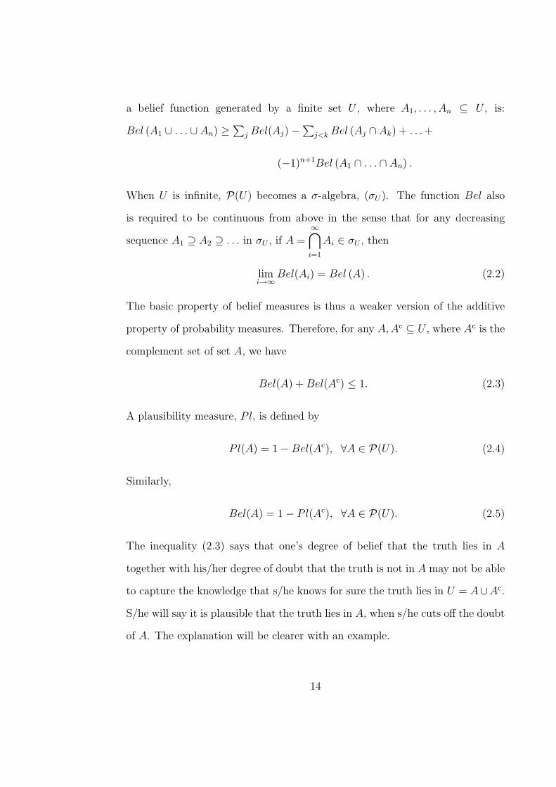
a belief function generated by a finite set U , where A1, . . . , An ⊆ U , is:

Bel (A1 ∪ . . . ∪ An) ≥∑

j Bel(Aj)−∑

j<k Bel (Aj ∩ Ak) + . . . +

(−1)n+1Bel (A1 ∩ . . . ∩ An) .

When U is infinite, P(U) becomes a σ-algebra, (σU). The function Bel also

is required to be continuous from above in the sense that for any decreasing

sequence A1 ⊇ A2 ⊇ . . . in σU , if A =∞⋂

i=1

Ai ∈ σU , then

limi→∞

Bel(Ai) = Bel (A) . (2.2)

The basic property of belief measures is thus a weaker version of the additive

property of probability measures. Therefore, for any A,Ac ⊆ U , where Ac is the

complement set of set A, we have

Bel(A) + Bel(Ac) ≤ 1. (2.3)

A plausibility measure, Pl, is defined by

Pl(A) = 1−Bel(Ac), ∀A ∈ P(U). (2.4)

Similarly,

Bel(A) = 1− Pl(Ac), ∀A ∈ P(U). (2.5)

The inequality (2.3) says that one’s degree of belief that the truth lies in A

together with his/her degree of doubt that the truth is not in A may not be able

to capture the knowledge that s/he knows for sure the truth lies in U = A∪Ac.

S/he will say it is plausible that the truth lies in A, when s/he cuts off the doubt

of A. The explanation will be clearer with an example.

14

Example 1. Consider an opinion poll for a Colorado governor’s election.

Let U = a, b, c, d, e be the set of candidates. There are 10,000 individuals

providing their preferences. They may not have made their final choice, since

the poll takes place well before the election. Suppose that 3,500 individuals

support candidates a and b from the Republican party, and 4,500 people support

candidates c, d, and e from the Democratic party. The remaining 2,000 persons

have no opinion yet. Therefore, we believe that one among the candidates from

the Democratic party will become the new governor with the degree of belief

0.45, and for those who prefer that a Republican candidate will win, they doubt

that the Democrat will win to the degree 0.35. That is, Dou(Democratic) =

Bel(Democraticc) = Bel(Republican) = 0.35. Combine the degree of belief and

the degree of doubt that the Democrat will win the Colorado governor election,

we obtain 0.45 + 0.35 = 0.70 < 1. It is also plausible that the Democrat will

win with 0.45+0.20 = 0.65 degree of plausibility when we assume that all 2,000

voters with no opinion finally choose one of the candidates from the Democratic

party. This 0.65 degree of plausibility is obtained when we subtract the 0.35

degree of doubt from the total belief of 1 that the new governor is a person in

the set U . ♦

Belief and plausibility measures also can be characterized by a basic prob-

ability assignment function m, which is defined on P(U) to [0, 1], such that

m(∅) = 0 and∑

A∈P(U)

m(A) = 1. (2.6)

It is important to understand the meaning of the basic probability assignment

function, and it is essential not to confuse m(A) with the probability of occur-

15

rence of an event A. The value m(A) expresses the proportion to which all

available and relevant evidence supports the claim that a particular element u

of U , whose characterization in terms of relevant attributes is deficient, belongs

to the set A. For Example 1, an element u can be referred to as a candidate

who will win the Colorado governor’s election, that is u ∈ a, b, c, d, e, where

m (a, b) = 0.35, m (c, d, e) = 0.45, and m(a, b, c, d, e) = 0.20. It is clear

that a, b and c, d, e are subsets of U = a, b, c, d, e, but m (a, b) and

m (c, d, e) are greater than m(U). Hence, it is allowed to have m(A) > m(B)

even if A ⊆ B.

The value m(A) pertains solely to the set A. It does not imply any addi-

tional claims regarding subsets of A. One also may see m(A) as the amount of

probability pending over elements of A without being assigned yet, by lack of

knowledge. If we had perfect probabilistic knowledge, then for every element u

in a finite set U , we would have m (u) = Pr (u), and∑

u∈U m (u) = 1.

Thus, m (A) = 0, when A is not a singleton subset of U . Here are some dif-

ferences between probability distribution functions and basic probability assign-

ment functions.

• When A ⊆ B, it is not required that m(A) ≤ m(B), while Pr(A) ≤ Pr(B).

• It is not required that m(U) = 1, while Pr(U) = 1.

• No relationship between m(A) and m(Ac) is required, while Pr(A) +

Pr(Ac) = 1.

A basic probability assignment function m is an abstract concept that helps

us create belief and plausibility measures. The reason to have such an abstract

16

concept is for the cases when the exact probability of all sets in the universe

is not known. When we do not know the probability on all elements of the

universe, but we have information on some collection of subsets, it is possible to

define a belief and a plausibility based on this information using the assignment

function. As long as we have an assignment function (2.6), we can construct

belief and plausibility functions (see (2.7) and (2.8) below).

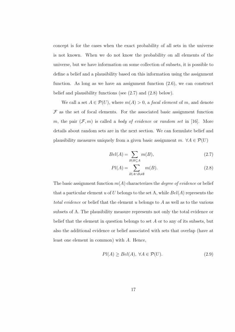
We call a set A ∈ P(U), where m(A) > 0, a focal element of m, and denote

F as the set of focal elements. For the associated basic assignment function

m, the pair (F ,m) is called a body of evidence or random set in [16]. More

details about random sets are in the next section. We can formulate belief and

plausibility measures uniquely from a given basic assignment m. ∀A ∈ P(U)

Bel(A) =∑

B|B⊆A

m(B), (2.7)

Pl(A) =∑

B|A∩B 6=∅

m(B). (2.8)

The basic assignment function m(A) characterizes the degree of evidence or belief

that a particular element u of U belongs to the set A, while Bel(A) represents the

total evidence or belief that the element u belongs to A as well as to the various

subsets of A. The plausibility measure represents not only the total evidence or

belief that the element in question belongs to set A or to any of its subsets, but

also the additional evidence or belief associated with sets that overlap (have at

least one element in common) with A. Hence,

Pl(A) ≥ Bel(A), ∀A ∈ P(U). (2.9)

17

Example 2. Consider the group of 2,000 individuals who did not have any

opinion at first, from Example 1. Suppose 500 of them admit that they will

vote for the candidate a, and the other 500 will vote for either b or d, but they

want to have a closer look before making final choice. Let A1 = a, b , A2 =

c, d, e , A3 = a, and A4 = b, d. Figure 2.1 shows the Venn diagram of

these sets. From this latest information, we obtain m(A1) = 0.35, m(A2) =

0.45, m(A3) = 0.05, m(A4) = 0.05, and m(U) = 0.10. Then, for instance,

Bel(A3) = m(A3) = 0.05, Bel(A1) = m(A1) + m(A3) = 0.40, and Pl(A1) =

m(A1) + m(A3) + m(A4) + m(U) = 0.55. ♦

3, 500 4, 500

500 1, 000 500

voters

b

a

d

c

e

A1 A2

A3

A4

candidates

U

Figure 2.1: Venn diagram of an opinion poll for a Colorado governor’s election.

The inverse procedure to get ‘m’ from ‘Bel’ is also possible. Given a belief

measure Bel, the corresponding basic probability assignment m is determined

for all A ∈ P(U) by the formula

m(A) =∑

B|B⊆A

(−1)|A−B|Bel(B). (2.10)

Hence, the basic probability assignment of the set A1 in Example 2 is m(A1) =

Bel(A1) − Bel(A3) = 0.40 − 0.05 = 0.35, as expected. The proof of (2.10) can

18

be found in Appendix A.

Now, we have enough material to develop some details of possibility theory.

A possibility measure is a plausibility in which all focal elements are nested. The

sets defined in Example 2 are not nested. Therefore, information for Example

2 is not considered to be possibility information. Let a possibility measure and

a necessity measure be denoted by the symbols Pos and Nec, respectively. The

basic properties of possibility theory are the result of the nestedness of focal

elements, and the proof can be found in Appendix B. These properties are as

follows: ∀A,B ∈ P(U)

Nec(A ∩B) = min Nec(A), Nec(B) , (2.11)

Pos(A ∪B) = max Pos(A), Pos(B) . (2.12)

However, no one has mentioned that if we have properties (2.11) and (2.12), then

the nestedness of focal elements is preserved. Therefore, we prove the stronger

statement (see Appendix B) that Bel(A ∩ B) = min Bel(A), Bel(B) , and

Pl(A ∪B) = max Pl(A), P l(B) if and only if the focal elements are nested.

The nestedness of focal elements guarantees that the meanings of necessity

and possibility are preserved as in (2.11) and (2.12). A possibility measure also

has a monotonicity property, which is in contrast with general basic probability

assignment functions. That is

if A ⊆ B, then Pos(A) ≤ Pos(B).

This monotonicity property is a result of (2.12). It can be interpreted as when

more evidence is provided, the possibility can never be lower than the possibility

when less evidence is given.

19

Necessity measures and possibility measures satisfy these following proper-

ties since they are a special case of belief and plausibility measures:

Nec(A) + Nec(Ac)≤ 1, (2.13)

Pos(A) + Pos(Ac)≥ 1, (2.14)

Nec(A) + Pos(Ac) = 1, (2.15)

min Nec(A), Nec(Ac)= 0, (2.16)

max Pos(A), Pos(Ac)= 1, (2.17)

Nec(A) > 0⇒ Pos(A) = 1, (2.18)

Pos(A) < 1⇒ Nec(A) = 0. (2.19)

The function pos : U → [0, 1] is defined on elements of the set U as

pos (u) = Pos(u), ∀u ∈ U, (2.20)

when a set-valued possibility measure Pos is given. It is called a possibility

distribution function associated with Pos. We can construct a set-valued pos-

sibility measure from a possibility distribution in the following way. For each

A ∈ P(U),

Pos(A) = supu∈A

pos (u) . (2.21)

Let us start the process of constructing a possibility distribution from a

basic probability assignment function m. This will help us to see the relationship

between possibility/necessity measures and random sets. For simplicity, consider

a set U = u1, u2, . . . , un. We will construct a possibility measure Pos defined

on P(U) in terms of a given basic probability assignment m. Without loss

20

of generality, assume that the focal elements are some or all of the subsets

in the sequence of nested subsets A1 ⊆ A2 ⊆ . . . ⊆ An = U, where Ai =

u1, u2, . . . , ui , i = 1, 2, . . . , n. We have

m (∅) = 0, andn∑

i=1

m(Ai) = 1.

However, it is not required that m(Ai) 6= 0 for all i = 1, 2, . . . , n. We define a

possibility distribution function for each ui ∈ U using Equation (2.8) as

pos (ui) = Pos(ui) =n∑

k=i

m(Ak), i = 1, 2, . . . , n. (2.22)

Written more explicitly, we have

pos (u1) = m(A1) + m(A2) + m(A3) + . . . + m(Ai) + m(Ai+1) + . . . + m(An)

pos (u2) = m(A2) + m(A3) + . . . + m(Ai) + m(Ai+1) + . . . + m(An)

...

pos (ui) = m(Ai) + m(Ai+1) + . . . + m(An)

...

pos (un) = m(An).

This implies

m(Ai) = pos (ui)− pos (ui+1). (2.23)

For example, suppose that n = 7. Figure 2.2 (see also in [74]) illustrates a

possibility distribution constructed from the associated basic assignment defined

as m(A1) = 0, m(A2) = 0.3, m(A3) = 0.4, m(A4) = 0, m(A5) = 0, m(A6) =

0.1, and m(A7) = 0.2. The mathematical differences (for finite sets) between

21

probability and possibility theories are summarized in Table 2.1, which can be

found in [74].

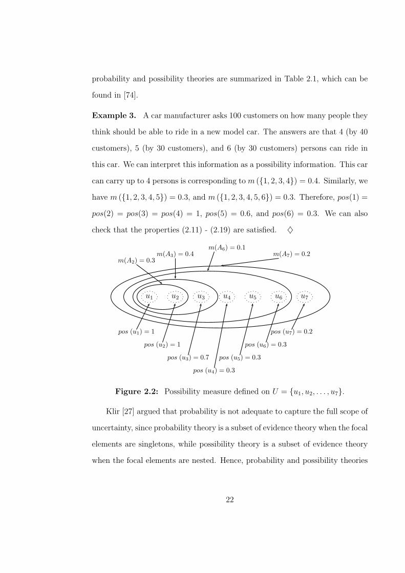
Example 3. A car manufacturer asks 100 customers on how many people they

think should be able to ride in a new model car. The answers are that 4 (by 40

customers), 5 (by 30 customers), and 6 (by 30 customers) persons can ride in

this car. We can interpret this information as a possibility information. This car

can carry up to 4 persons is corresponding to m (1, 2, 3, 4) = 0.4. Similarly, we

have m (1, 2, 3, 4, 5) = 0.3, and m (1, 2, 3, 4, 5, 6) = 0.3. Therefore, pos(1) =

pos(2) = pos(3) = pos(4) = 1, pos(5) = 0.6, and pos(6) = 0.3. We can also

check that the properties (2.11) - (2.19) are satisfied. ♦

u1

pos (u1) = 1

u2

pos (u2) = 1

u3

pos (u3) = 0.7

u4

pos (u4) = 0.3

u5

pos (u5) = 0.3

u6

pos (u6) = 0.3

u7

pos (u7) = 0.2

m(A2) = 0.3m(A3) = 0.4

m(A6) = 0.1m(A7) = 0.2

Figure 2.2: Possibility measure defined on U = u1, u2, . . . , u7.

Klir [27] argued that probability is not adequate to capture the full scope of

uncertainty, since probability theory is a subset of evidence theory when the focal

elements are singletons, while possibility theory is a subset of evidence theory

when the focal elements are nested. Hence, probability and possibility theories

22

are the same only when the body of evidence consists of one focal element that

is a singleton.

Table 2.1: Probability theory versus possibility theory: comparison of math-ematical properties for finite sets

Probability Theory Possibility Theory

Based on measures of one type: Based on measures of two types: Possibility

Probability measures, Pr measures, Pos and Necessity measures, Nec

Body of evidence consists of singletons Body of evidence consists of a family of nested subsets

Unique representation of Pr by a probability Unique representation of Pos by a possibility

density function pr : U → [0, 1] via distribution function pos : U → [0, 1] via

the formula Pr(A) =∑

u∈A

pr(u) the formula Pos(A) = maxu∈A

pos(u)

Normalization:∑

u∈U

pr(u) = 1 Normalization: maxu∈U

pos(u) = 1

Additivity: Max rule: Pos(A ∪ B) = max Pos(A), Pos(B)

Pr(A ∪ B) = Pr(A) + Pr(B) − Pr(A ∩ B) Min rule: Nec(A ∩ B) = min Nec(A), Nec(B)

Nec(A) = 1 − Pos(Ac)

Not applicable Pos(A) < 1 ⇒ Nec(A) = 0

Nec(A) > 0 ⇒ Pos(A) = 1

Pos(A) + Pos(Ac) ≥ 1 ; Nec(A) + Nec(Ac) ≤ 1

Pr(A) + Pr(Ac) = 1 max Pos(A), Pos(Ac) = 1

min Nec(A), Nec(Ac) = 0

Total ignorance: pr(u) =1

|U |for all u ∈ U Total ignorance: pos(u) = 1 for all u ∈ U

The nestedness property in possibility theory guarantees the maximum ax-

iom (rather than additivity axiom in probability theory). Therefore, these two

theories are not contained in one another; they are distinct. Moreover, proba-

bility and possibility theories involve different types of uncertainty and should

be applied differently. For example, probability is suitable for characterizing the

number of persons that are expected to ride in a particular car each day. Pos-

23

sibility theory, on the other hand, is suitable for characterizing the number of

persons that can ride in that car at any one time. Since the physical characteris-

tics of persons such as size or weight are intrinsically vague, it is not realistic to

describe the situation by sharp probabilistic distinctions between possible and

impossible instances. The readers who interest in more discussion can find full

details in [27].

We explained how a basic probability assignment function m relates to belief

and plausibility functions, given a finite set U . In the next section, the math-

ematical definition of random sets and some examples that help understanding

the definition of random sets are provided. Theorem 2.14 shows that the belief

(plausibility) and the necessity (possibility) functions are the same, when the

focal elements are nested, (regardless the cardinality of U). We prove that be-

lief and plausibility measures are the bounds on a set of probability measures

generated by a random set. Finally, we show how to find the smallest and the

largest expected values of a random variable with unknown probability from a

given random set.

2.2 Random sets

We introduced in the previous section a random set as a body of evidence

when U is a finite set of realizations. In this section, we give a more solid

mathematical definition of a random set. Although, we limit the scope of this

dissertation to a finite set U , it is worth explaining random sets in this section as

generally as possible, so that we have some useful material for future research. A

random set is a random variable such that an element in its range is a subset of a

set X (finite or infinite). The differences between random variables and random

24

sets from their definitions can be seen in Definitions 2.4 and 2.5. First of all,

we provide the definitions of a σ-algebra, a measurable space, a measurable

mapping, and a probability space, which will be used in the definitions of a

random variable and a random set. Definitions 2.1 - 2.3 can be found in any

measure theory book.

Definition 2.1 Let Ω be a non-empty set. A σ-algebra on Ω, denoted by σΩ,

is a family of subsets of Ω that satisfies the following properties:

• ∅ ∈ σΩ,

• B ∈ σΩ ⇒ Bc ∈ σΩ, and

• Bi ∈ σΩ, for any countable (or finite) subset Bi of σΩ ⇒ ∪i Bi ∈ σΩ.

A pair (Ω, σΩ) is called a measurable space.

Definition 2.2 Let (Ω, σΩ) be a measurable space. By a measure on this space,

we mean a function µ : σΩ → [0,∞] with the properties:

• µ (∅) = 0, and

• if Bi ∈ σΩ, ∀ i = 1, 2, . . . , are disjoint, then µ

(∞⋃

i=1

Bi

)=

∞∑

i=1

µ(Bi).

We refer to the triple (Ω, σΩ, µ) as a measure space. If µ (Ω) = 1, we refer to it

as a probability space and write it as (Ω, σΩ, P rΩ), where PrΩ is a probability

measure.

Definition 2.3 Let (Ω, σΩ) and (U, σU) be measurable spaces. A function

f : Ω → U is said to be a (σΩ, σU)-measurable mapping if f−1(A) =

ω ∈ Ω : f(ω) ∈ A ∈ σΩ, for each A ∈ σU .

25

Definition 2.4 (see Marın [43]) Let (Ω, σΩ, P rΩ) be a probability space and

(U, σU) be a measurable space. A random variable X is a (σΩ, σU)-measurable

mapping

X : Ω→ U. (2.24)

This mapping can be used to generate a probability measure on (U, σU). The

probability PrU(A) for an event A ∈ σU is given by

PrU(A) = PrΩ

(X−1(A)

)= PrΩ (ω ∈ Ω : X(ω) ∈ A) , (2.25)

where ω ∈ Ω : X(ω) ∈ A ∈ σΩ.

It follows that, for A ∈ σU ,

PrU(A) :=∑

ω∈X−1(A)

PrΩ(ω) (discrete case) (2.26)

:=

∫

X−1(A)

dPrΩ(ω)︸︷︷︸c.d.f.

(continuous case), (2.27)

where c.d.f. stands for cumulative distribution function. PrΩ(ω) in (2.27) is the

cumulative distribution with respect to Ω , when ω ∈ Ω, while PrΩ(ω) is the

probability measure on ω, which is an element in σΩ.

Example 4. Let Ω be the set of all outcomes of tossing two fair dice, i.e.,

Ω = (1, 1), (1, 2), . . . , (6, 6), with the probability PrΩ ((i, j)) = 136

, where

i, j = 1, 2, . . . , 6. A mapping from Ω to the sum of each outcome is a random

variable X : (i, j) 7→ i + j, where the set U = 2, 3, . . . , 12. The sets σΩ and

σU are the power set of Ω and U , respectively. Let A ∈ σU . Then PrU(A) =

PrΩ ((i, j) ∈ Ω : X((i, j)) ∈ A). For instance, suppose A = 2, 12, then

PrU (2, 12) = PrΩ ((1, 1), (6, 6)) = 236

. ♦

26

Definition 2.5 (see Marın [43]) Let (Ω, σΩ, P rΩ) be a probability space and

(F , σF) be a measurable space, where F ⊆ σU , U 6= ∅, and (U, σU) is a measur-

able space. A random set Γ is a (σΩ, σF)-measurable mapping

Γ : Ω→ F (2.28)

ω 7→ Γ(ω).

We can generate a probability measure on (F , σF) by using the probability mea-

sure m(R) = PrΩ ω : Γ(ω) ∈ R, where R ∈ σF . Therefore, when F is finite

and σF is the power set of F , we have∑

γ∈F

m(γ) = 1. Finally, we use the

notation (F ,m) to represent a finite or infinite random set depending on

the cardinality of F .

Remark 2.6 The probability m in Definition 2.5 is called a basic probability

assignment function, which is distinct from a ‘regular’ probability on U . A basic

probability assignment function is actually a probability on σU .

Remark 2.7 In practice, the set F can be given so that m(γ) > 0, for all

γ ∈ F . For ω ∈ Ω, a set γ := Γ(ω) ∈ F is called a focal element if m(γ) > 0.

A set γ |m(γ) > 0 is called a focal set.

Remark 2.8 Γ becomes a random variable: Γ(ω) = U(ω), when U is a finite

non-empty set and all elements of F are singletons, i.e. F = u : u ∈ U.

However, we cannot know the exact value of PrU(A) for any A ∈ σU ,in general,

when we have information in the terms of random sets, because elements of F

can be any subsets of U .

27

There are two cases that generate a finite random set: 1) when U is finite,

we have that F is finite, and 2) when U is infinite (discrete or continuous), but

F is finite. Hence, there are a finite number of focal elements. Each of them

can be a finite or an infinite set. An infinite random set is generated from an

infinite set U , which also can be digested into two situations: 1) when U is

infinite discrete, and 2) when U is a continuous set. Each of an infinite number

of focal elements of an infinite random set can be either finite or infinite. The

following examples help us understand the definition of random sets.

Example 5. Finite random set when U is finite.

Let us revisit Example 1. Consider an opinion poll for a Colorado governor’s

election. The set of candidates is U = a, b, c, d, e. There is a population Ω

of 10, 000 individuals that provide their preferences. They may not have made

a final choice, since the poll takes place well before the election. The opinion

of individual ω ∈ Ω is modeled by Γ(ω) ⊆ U . Therefore, each person ‘ω’ of

3,500 Republican supporters is modeled by Γ(ω) = a, b, each person ‘ω’ of

4,500 Democrat supporters is modeled by Γ(ω) = c, d, e, and each person

‘ω’ of 2,000 undecided individuals is modeled by Γ(ω) = a, b, c, d, e = U .

Hence, the finite random set (F ,m) is when F = a, b , c, d, e , U, such

that m (a, b) = 0.35, m (c, d, e) = 0.45, and m (U) = 0.20, where

m(γ) is the proportion of opinions of the form Γ(ω) = γ. ♦

Remark 2.9 If we use different group of 15, 000 people to provide the survey

for Example 5 (different information), we may obtain a totally different random

set from what we got in Example 5. Therefore, we need to be clear about the

28

sample space Ω we are using. However, if we add these 15, 000 people to the

other 10, 000 that we asked for the survey (more information), we will increase

the size of the sample space Ω, but the updated belief (or plausibility) still could

be less than, greater than or equal to the belief (or plausibility) got from random

set in Example 5, depends upon the survey of these 15, 000 people.

On the other hand, consider the random set information for Example 5,

this time we receive more details on those of 4, 500 who support Republican

candidates that 2, 000 will vote for candidate c, and other 2, 500 still do not have

final decision, so each of their votes could go to one of either c, d, or e. In

this case, the new information is based on the old information, but more specific

on who will vote for c. It should not difficult to see that the updated belief will

be greater than or equal to the belief from the old information. Moreover, the

updated plausibility will be less than or equal to the old plausibility.

Remark 2.10 We provided an example of a coin where its fairness is in ques-

tion, at the beginning of this chapter. This coin has random set information as

follows. Let H := head, and T := tail. Then, Ω = H,T with PrΩ H,T = 1.

The set U also is H,T, which is the only focal element for the random set,

i.e., m(U) = m(H,T) = 1. Therefore, Bel(H) = Bel(T) = 0, and

Pl(H) = Pl(T) = 1. However, if we flip this coin 100, 000 times and it

turns head for 43, 000 times (turns tail for 57, 000 times), this information is dif-

ferent from the information PrΩ H,T = 1. Therefore, the clarification of the

set Ω is very important in the conclusion of Bel and Pl values. For this exper-

iment, Ω refers to the setflip1,flip2 . . . ,flip100,000

, with PrΩ(flipi) = 10−5.

The set U = H,T, with m(H) = 0.43 and m(T) = 0.57. Since, the

29

focal elements now are singleton, we can conclude that Bel(H) = Pl(H) =

PrU(H) = 0.43, and Bel(T) = Pl(T) = PrU(T) = 0.57. Based on

these 100, 000 trials, the probability (experiment based) of a head is 0.43, and

the probability (experiment based) of a tail is 0.57. This probability is based on

the experiment, and we will use it to represent this coin when the only infor-

mation we have is this experiment. It may over and/or under estimate the real

probability of this coin.

We conclude the thought from Remarks 2.9 and 2.10 as follows: 1) the

clarification of the set Ω is important for the conclusion of Bel and Pl values,

and 2) if we receive more information by digesting the old information to become

more specific, then Belold(A)) ≤ Belupdated(A)) ≤ Plupdated(A)) ≤ Plold(A)).

Example 6. Finite random set when U is infinite.

A round target is spinning with an unknown speed and placed in a dark room.

It also has numbers 0, π2, π, and 3π

2to indicate all angles in [0, 2π). John throws

a dart to this target for a total of 1,000 trials. The result he delivers is that

the darts on the pie areas between[0, 3π

4

),[

3π4

, 3π2

), and (3π

2, 2π) of total 350,

467, and 233, respectively. To be consistent with Definition 2.5, we consider

Ω = ω | ω = 1, 2, . . . , 1, 000, representing trial number 1, 2, . . . , 1, 000, where

PrΩ(ω) = 11,000

. We also have U = [0, 2π) and F =[

0, 3π4

),[

3π4

, 3π2

), (3π

2, 2π)

.

The information John provided can be represented as m([

0, 3π4

)) = 0.350,

m([

3π4

, 3π2

)) = 0.467, and m(

(3π

2, 2π)

) = 0.233. This information is not

enough to be able to know that the proportion that the dart will lie on a selected

area, e.g., the area between [π4, π

3], for the next trial. However, we can say that

the dart will point on the pie area between [π4, π

3] with plausibility of 0.350. ♦

30

Example 7. Infinite random set.

An urn contains N white and M black balls. Balls are drawn randomly, one at a

time, until a black one is drawn. If we assume that each selected ball is replaced

before the next one is drawn, each of these independent draws has probability

p = MN+M

for being a success (a black ball is drawn). Let Ω be the set of the

number of draws needed to obtain a black ball, i.e., Ω = ω : ω = 1, 2, 3, . . .

with probability PrΩ(n) = p (1− p)n−1, where n = 1, 2, 3, . . .. In addition, we

have a round target as in Example 6. This time, John provides the information

that he can relate the number of draws until getting a black ball and a pie area

that the dart will hit as follows:

ω = 1⇒ the dart can lies somewhere in the pie area [0, π] ⇒ Γ(1) = [0, π],

ω = 2⇒ the dart can lies somewhere in the pie area [0, 3π2

] ⇒ Γ(2) = [0, 3π2

],

ω = 3⇒ the dart can lies somewhere in the pie area [0, 7π4

] ⇒ Γ(3) = [0, 7π4

],

and so on. Thus, U = [0, 2π], and F =[

0, (2n−1)π2n−1

]; n = 1, 2, 3, . . .

. Hence,

m([

0, (2n−1)π2n−1

])= p (1− p)n−1, and

∑∞n=1 m

([0, (2n−1)π

2n−1

])= 1. What is

the probability that the dart lies somewhere in the pie area [9π5

, 11π6

]? We cannot

get the answer for this question with the information we have. The only thing

we can say is that the dart may lie in the pie area [9π5

, 11π6

] with the degree of

possibility 1−∑3

n=1 p(1− p)n − 1. ♦

Let U be a finite set, F be the power set of U , σF be the power set of F ,

and m be a probability basic assignment function on σF . The other versions of

the belief and plausibility measures for a finite random set, given a finite set U ,

31

can be derived as: ∀ A ⊆ U,

Bel(F ,m)(A) =∑

γi⊆A

γi∈F

m(γi) (2.29)

= m (γi : γi ⊆ A, γi 6= ∅) (2.30)

= PrΩ ω : Γ(ω) ⊆ A, Γ(ω) 6= ∅ , (2.31)

and

Pl(F ,m)(A) =∑

γi∩A 6=∅

γi∈F

m(γi) (2.32)

= m (γi : γi ∩ A 6= ∅) (2.33)

= PrΩ ω : Γ(ω) ∩ A 6= ∅ , (2.34)

We add the subscript (F ,m) of Bel and Pl functions to make clear that these

functions are based on the random set (F ,m). A random set (F ,m) can be a

finite random set even when U is infinite. The belief and plausibility formulas

for a finite random set, with respect to a random set whose U is infinite, are

the same as (2.29 - 2.34). We will sometimes say (F ,m) is a finite random set

without mentioning the cardinality of U . An infinite random set can happen

when U is an infinite set. The belief and plausibility measures of any set A ⊆ U

for an infinite random set also are provided by (2.30 - 2.31) and (2.33 - 2.34),

respectively.

Next we will use a continuous possibility distribution pos(u) on U ⊆ Rn,

when U is a continuous set, to represent an infinite random set (F ,m), where

F is the family of all α-cuts Aα = u ∈ U : pos(u) ≥ α, α ∈ (0, 1].

32

Definition 2.11 Let U be a continuous subset of R. For a given continuous pos-

sibility distribution pos(u) on U ⊆ R, we define (F ,m) as an infinite random

set generated by ‘pos’, where F := Aα : α ∈ (0, 1]. Let G ⊆ (0, 1], and

R = Aα : Aα ∈ F , α ∈ G. The corresponding basic probability assignment

m : σF → [0, 1] is induced as

m (R) =

∫

R

dm(γ) =

∫

G

dPr(α) = Pr(G), (2.35)

where Pr is the probability measure on R corresponding to the uniform cu-

mulative distribution function. That is, Pr(α ≤ α) = α; α ∈ [0, 1], where

α represents the random variable, and α is its realization. Furthermore, let-

ting n ∈ N, we use (Fn,mn) as a finite representation of this infi-

nite random set (F ,m) by discretizing [0, 1] into n subintervals, where

Fn =

A in

: i = 1, 2, . . . , n, and mn

(A i

n

)= 1

n. We also can see that

∑n

i=1 mn

(A i

n

)= 1.

A i+1n

A in

mn

(A i+1

n

)= i+1

n− i

n= 1

n

i+1ni

n

Figure 2.3: A finite representation of an infinite random set.

A finite representation of an infinite random set given a possibility distribution

is illustrated in Figure 2.3. The belief and plausibility measures for a finite

representation (Fn,mn) of (F ,m) are given by

Bel(Fn,mn)(A) =∑

A in⊆A

mn

(A i

n

), and Pl(Fn,mn)(A) =

∑

A in∩A 6=∅

mn

(A i

n

).

33

Theorem 2.12 (The strong law of large numbers, [2]) Let X1, X2, . . . be a se-

quence of independent and identically distributed random variables, each having

a finite mean µ = E[Xi]. Then

limn→∞

X1 + X2 + . . . + Xn

n→ µ, almost surely. (2.36)

The strong law of large numbers is used in the proof of Theorem 2.13.

Theorem 2.13 (see Marın [43]) Let (Fn,mn) be a finite representation of an

infinite random set (F ,m) as defined in the Definition 2.11. The belief (and

plausibility) of the random set (Fn,mn) converges almost surely to the belief

(and plausibility) of the random set (F ,m) as n→∞, i.e.,

Bel(F ,m)(A) = limn→∞

Bel(Fn,mn)(A), and (2.37)

Pl(F ,m)(A) = limn→∞

Pl(Fn,mn)(A), (2.38)

almost surely, ∀A ∈ σU .

The next theorem tells us that in general, if the focal elements are nested

(regardless of the cardinality of the focal set F), then the belief measure is the

necessity measure, and the plausibility measure is the possibility measure.

Theorem 2.14 (see Marın [43]) Let (Fn,mn) be a finite representation of an

infinite random set (F ,m) as defined in the Definition 2.11. Then

NecU(A) = Bel(F ,m)(A) = limn→∞

Bel(Fn,mn)(A), and (2.39)

PosU(A) = Pl(F ,m)(A) = limn→∞

Pl(Fn,mn)(A), (2.40)

almost surely, ∀A ∈ σU .

34

We skip the proofs of Theorems 2.13 and 2.14. The readers can view the proofs

from [43]. Theorems 2.13 and 2.14 will be useful for future research, when we

consider the continuous case of U .

Let us define the setMi of probability measures associated with Ai as

Mi =Pri : σU → [0, 1] | Pri(A) = 1, whenever Ai ⊆ A, A ∈ σU

.

A finite random set (F ,m) can be interpreted as the set of probability measures,

MF , of the form MF =

Pr : Pr(A) =∑L

i=1 m(Ai)Pri(A), A ∈ σU

, where

each P i belongs to the set Mi of probability measures on Ai, as claimed by

many authors, see [16] for example. Many papers, e.g. [13, 16, 55, 56], claim

that for all A ∈ σU , Bel(A) ≤ Pr(A) ≤ Pl(A), ∀Pr ∈ MF . We state the

theorem and proof here. The details are as follows. The term m(γ) will be

written as m(γ), ∀ γ ∈ F in the rest of the dissertation, for convenience.

Theorem 2.15 Let u be an uncertainty with a set of realizations U , where U

can be finite or infinite, and σU is given. Suppose that (F ,m) is a finite random

set of u, where the focal set is F = Ai ∈ σU, i = 1, 2, . . . , L, for some L ∈ N.

Then, the random set can be interpreted as the unique set of probability measure

MF of the form

MF =

Pr | Pr(A) =

L∑

i=1

m(Ai)Pri(A), A ∈ σU

, (2.41)

where each Pri belongs to the setMi of probability measures associated with Ai,

such that for all A ∈ σU , Bel(A) ≤ Pr(A) ≤ Pl(A), ∀Pr ∈MF . Additionally,

we have infPr∈MF

Pr(A) = Bel(A), and supPr∈MF

Pr(A) = Pl(A).

Proof: Please note that Pri is an arbitrary element of Mi. First, we verify

that Pr in (2.41) satisfies the probability axioms as follows:

35

• Since m(Ai) and Pri(A) are in [0, 1], for each Ai ∈ F , A ∈ σU , and

Pri ∈Mi, 0 ≤ Pr(A) =∑L

i=1 m(Ai)Pri(A) ≤ 1.

• Pr(U) =∑L

i=1 m(Ai) = 1, because Pri(U) = 1 for all Pri ∈ Mi, i =

1, 2, . . . , L.

• For any A1, A2 ∈ σU such that A1

⋂A2 = ∅,

P r(A1

⋃A2) =

∑I

i=1 m(Ai)Pri(A1

⋃A2)

=∑L

i=1 m(Ai) (Pri(A1) + Pri(A2))

=∑L

i=1 m(Ai)Pri(A1) +∑L

i=1 m(Ai)Pri(A2)

= Pr(A1) + Pr(A2).

Define Pr(A) = infPr∈MF

Pr(A) and Pr(A) = supPr∈MF

Pr(A), therefore

Pr(A) = inf

Pr(A) =

L∑

i=1

m(Ai)Pri(A), P ri ∈Mi

, A ∈ σU , and

Pr(A) = sup

Pr(A) =

L∑

i=1

m(Ai)Pri(A), P ri ∈Mi

, A ∈ σU .

We note that these two functions may not follow the axioms of probability. We

can see that for a given A ∈ σU , the value of∑L

i=1 m(Ai)Pri(A) depends on

the value of Pri(A). Therefore,∑L

i=1 m(Ai)Pri(A) is the smallest value when

Pri(A) = 0, as long as it does not violate the restriction of the setMi. It is not

hard to see that a specific probability measure Pri1, for each i = 1, 2, . . . , L,

Pri1(A) =

1; if Ai ⊆ A,

0; otherwise,

provide

Pr(A) =∑

Ai⊆A

m(Ai) = Bel(A).

36

Similarly,∑L

i=1 m(Ai)Pri(A) is the largest value when Pri(A) = 1, as long as it

does not violate the restriction of the setMi. If this set A is such that Ai∩A = ∅

and Pri(A) > 0, it implies that Pri(Ai) < 1, since Pri(Ai) = 1−Pri(A). Hence

this Pri /∈ Mi. Therefore, Pri(A) = 0, when Ai ∩ A = ∅, and Pri ∈ Mi.

Moreover, if Ai∩A 6= ∅, there is Pri ∈Mi such that Pri(A) = 1 = Pri(Ai∩A),

because this Pri satisfies Pri(B) = 1, whenever Ai ⊆ B (i.e., Ai ∩ B 6= ∅).

Hence,

Pr(A) =∑

Ai⋂

A 6=∅

m(Ai) = Pl(A),

by using a specific probability measure Pri2, for each i = 1, 2, . . . , L,

Pri2(A) =

1; if Ai ∩ A 6= ∅,

0; otherwise.

Next, we show that MF is the unique set of probability measures that has

property Bel(A) ≤ Pr(A) ≤ Pl(A), ∀A ∈ σU . Suppose that P : σU → [0, 1]

is a probability measure such that Bel(A) ≤ P (A) ≤ Pl(A), ∀A ∈ σU . Let

A ∈ σU . Then,

Bel(A) =L∑

i=1

m(Ai)Pri1(A) ≤ P (A) ≤

L∑

i=1

m(Ai)Pri2(A) = Pl(A).

Without loss of generality, we suppose that there exists l ≤ L such that Ai ⊆ A,

for each i = 1, 2, . . . , l. Therefore, Bel(A) =l∑

i=1

m(Ai) =l∑

i=1

m(Ai)Pri1(A).

Since Ai * A, for all i = l + 1, l + 2, . . . , L, we suppose further that there exists

l < k ≤ L such that Ai ∩ A 6= ∅, for all i = l + 1, l + 2, . . . , k. Hence,

Bel(A) =l∑

i=1

m(Ai)Pri1(A) ≤ P (A) ≤

k∑

i=1

m(Ai)Pri2(A) = Pl(A).

37

If l = k, then l = k = L and P (A) = Bel(A) = Pl(A). We are done. Otherwise,

set a = P (A) − Bel(A) > 0. Pri(A) =a

(k − l)m(Ai)= Pri(A ∩ Ai), ∀ i =

l + 1, l + 2, . . . , k, does not violate the restriction ofMi. Thus, this Pri ∈ Mi,

for each i = l+1, l+2, . . . , k. Moreover, Pri(A) = 0, ∀ i = k+1, k+2, . . . , L also

does not violate the restriction ofMi, i = k + 1, k + 2, . . . , L, since Ai ∩A = ∅.

Hence,

P (A) = Bel(A) + a + 0

=l∑

i=1

m(Ai)Pri1(A) + m(Al+1)Prl+1(A) + . . . + m(Ak)Prk(A) +

m(Ak+1)Prk+1(A) + . . . m(AL)PrL(A)

satisfies Bel(A) ≤ P (A) ≤ Pl(A), ∀A ∈ σU and is in the form of (2.41).

It follows from Theorems 2.13 and 2.14 that infPr∈MF

Pr(A) and supPr∈MF

Pr(A),

where MF is interpreted from a (finite or infinite) random set induced by a

possibility distribution are belief and plausibility of A, ∀A ∈ σU . We state this

result in the following Corollary 2.16.

Corollary 2.16 Assume

H1: (Ω, σΩ, P rΩ) is a probability space,

H2: U is an arbitrary set of consideration, and

H3: (F ,m) is a random set generated by a possibility distribution.

Then, we have the same conclusion as in Theorem 2.15.

Theorem 2.15 and Corollary 2.16 mean that a random set (F ,m) can be inter-

preted as a set of probability measures MF whose bounds on probability are

38

belief and plausibility measures. By these bounds, we can find a probability

density mass function that generates the smallest (largest) expected value of

our random variable.

2.2.1 Upper and lower expected values generated by random sets

Given a random set (F ,m) of U = u1, u2, . . . , un, and an evaluation func-

tion θ of U , where θ(u1) ≤ θ(u2) ≤ . . . ≤ θ(un), the lowest and the largest

expected values of θ can be evaluated by using the following density functions

f and f of a random variable U : Ω→ U ,

where f(u1) = Bel(u1, u2, . . . , un)−Bel(u2, u3 . . . , un)

...

f(ui) = Bel(ui, ui+1, . . . , un)−Bel(ui+1, ui+2, . . . , un)...

f(un) = Bel(un),

(2.42)

and

f(u1) = Bel(u1)

...

f(ui) = Bel(u1, u2, . . . , ui)−Bel(u1, u2, . . . , ui−1)...

f(un) = Bel(u1, u2, . . . , un)−Bel(u1, u2, . . . , un−1).

(2.43)

These two functions f and f are indeed density functions because each of them

sums to 1, and are nonnegative. They are important because they are density

functions that create the smallest and largest expected values E(θ), respectively.

We define Prg as a probability measure generated by a density function g.

It was proved in [54] by Nguyen that f in (2.42) provides the smallest expected

value of θ. We combine his proof together with our contribution to show that f

39

in (2.43) provides the largest expected value in Theorem 2.17 below. Example

8 illustrates the use of Theorem 2.17.

Theorem 2.17 For a given random set (F ,m) of U = u1, u2 . . . , un, let

θ : U → R be such that θ(u1) ≤ θ(u2) ≤ . . . ≤ θ(un), and Ef (θ) be an expected

value of the evaluation θ with respect to the density mass function f . Then

the density functions f and f defined in Equations (2.42) and (2.43) have the

property that

Ef (θ) = inf Ef (θ) : Prf ∈MF (2.44)

Ef (θ) = sup Ef (θ) : Prf ∈MF , (2.45)

where f and f ∈MF , and MF is defined by Theorem 2.15.

Proof : We first show that Prf and Prf are in MF . From (2.42) and (2.43),

we have

f(ui) = Bel(ui, ui+1, . . . , un)−Bel(ui+1, ui+2, . . . , un)

=∑

B⊆ui,ui+1,...,un

m(B)−∑

B⊆ui+1,ui+2,...,un

m(B)

=∑

B⊆ui,ui+1,...,un,ui∈B

m(B),

and f(ui) = Bel(u1, u2, . . . , ui)−Bel(u1, u2, . . . , ui−1)

=∑

B⊆u1,u2,...,ui

m(B)−∑

B⊆u1,u2,...,ui−1

m(B)

=∑

B⊆u1,u2,...,uiui∈B

m(B).

Let A =ui, ui+k1 , . . . , ui+kj

, then

Prf (A) =∑

ui∈A

f(ui) =∑

m(B)B⊆ui,...,un

ui∈B

+∑

m(B)

B⊆ui+k1,...,un

ui+k1∈B

+ . . . +∑

m(B)

B⊆ui+kj,...,un

ui+kj∈B

. (2.46)

40

We will show that Prf (A) ≥ Bel(A) =∑

B⊆A

m(B). Let B ⊆ A.

• If ui ∈ B, then m(B) is included in the first term of (2.46).

• If ui /∈ B, and ui+k1 ∈ B, then m(B) is included in the second term of

(2.46).

...

• If ui, ui+k1 , . . . , ui+kj−1/∈ B, and ui+kj

∈ B, then m(B) is included in the

last term of (2.46).

Hence, Prf (A) ≥ Bel(A). Moreover, since B ∩ A 6= ∅ for each set B in any

terms of (2.46), Prf (A) ≤ Pl(A). Therefore, Prf ∈MF . Likewise,

Prf (A) =∑

ui∈A

f(ui) =∑

m(B)B⊆u1,...,ui

ui∈B

+∑

m(B)

B⊆u1,...,ui+k1ui+k1

∈B

+ . . . +∑

m(B)

B⊆u1,...,ui+kjui+kj

∈B

. (2.47)

We will show that Prf (A) ≥ Bel(A) =∑

B⊆A

m(B). Let B ⊆ A.

• If ui+kj∈ B, then m(B) is included in the last term of (2.47).

• If ui+kj/∈ B, and ui+kj−1

∈ B, then m(B) is included in the second last

term of (2.47).

...

• If ui+kj, ui+kj−1

, . . . , ui+k1 /∈ B, and ui ∈ B, then m(B) is included in the

first term of (2.47).

Hence, Prf (A) ≥ Bel(A). Moreover, since B ∩ A 6= ∅ for each set B in any

terms of (2.47), Prf (A) ≤ Pl(A). Therefore, Prf ∈MF .

To prove (2.44) and (2.45), we apply the well-known expected value formula

(see [54] and [59]),

Ef (θ) =

∫ ∞

0

Prf (u | θ(u) > t) d t +

∫ 0

−∞

(Prf (u | θ(u) > t)− 1) d t. (2.48)

41

Let u | θ(u) > t = ui, ui+1, . . . , un, for some i = 1, 2, . . . , n. We know that

Prf (u | θ(u) > t) = Prf (ui, . . . , un) =n∑

j=i

f(uj) = Bel(ui, . . . , un)(2.49)

Prf (u | θ(u) > t) = Prf (ui, . . . , un) =n∑

j=i

f(uj) = Pl(ui, . . . , un).(2.50)

The last equality of (2.50) holds, since

n∑

j=i

f(uj) = (Bel(u1, u2, . . . , ui)−Bel(u1, u2, . . . , ui−1)) +

(Bel(u1, u2, . . . , ui+1)−Bel(u1, u2, . . . , ui)) + . . . +

(Bel(u1, u2, . . . , un)−Bel(u1, u2, . . . , un−1))

= Bel(u1, u2, . . . , un)−Bel(u1, u2, . . . , ui−1)

= 1−Bel(u1, u2, . . . , ui−1)

= Pl(ui, ui+1 . . . , un).

By Theorem 2.15, for every Prf ∈MF ,

Prf (u | θ(u) > t) ≤ Prf (u | θ(u) > t) ≤ Prf (u | θ(u) > t).

Without loss of generality, suppose that there exists k < n such that θ(uk) < 0

and θ(uk+1) ≥ 0. We divide t into the following subintervals

• t ∈ (−∞, θ(u1)) ⇒ u | θ(u) > t = U,

• t ∈ [θ(u1), θ(u2)) ⇒ u | θ(u) > t = u2, u3, . . . , un ,

...

• t ∈ [θ(uk−1), θ(uk)) ⇒ u | θ(u) > t = uk, uk+1, . . . , un ,

• t ∈ [θ(uk), 0) ⇒ u | θ(u) > t = uk+1, uk+2, . . . , un ,

42

• t ∈ [0, θ(uk+1)) ⇒ u | θ(u) > t = uk+1, uk+2, . . . , un ,

...

• t ∈ [θ(un−1), θ(un)) ⇒ u | θ(u) > t = un ,

• t ∈ [θ(un),∞) ⇒ u | θ(u) > t = ∅.

Applying f to (2.48), we have

Ef (θ) =

∫ ∞

0

Prf (u | θ(u) > t) d t +

∫ 0

−∞

(Prf (u | θ(u) > t)− 1) d t

= M1 + M2, where

M1 =

∫ θ(uk+1)

0

Bel(uk+1, uk+2, . . . , un) d t + . . . +

∫ θ(un)

θ(un−1)

Bel(un) d t +

∫ ∞

θ(un)

Bel(∅) d t.

M2 =

∫ θ(u1)

−∞

(Bel(U)− 1) d t +

∫ θ(u2)

θ(u1)

(Bel(u2, u3, . . . , un)− 1) d t

+ . . . +

∫ θ(uk)

θ(uk−1)

(Bel(uk, uk+1, . . . , un)− 1) d t

+

∫ 0

θ(uk)

(Bel(uk+1, uk+2, . . . , un)− 1) d t.

We can see that M1 is the smallest positive value and M2 is the largest negative

value associated with random set information. Hence Equation (2.44) hold.

Similarly, we also can apply f to (2.48), and obtain that Equation(2.45) holds.

Example 8. Let Ω be the set of outcomes from tossing a die where we know

only PrΩ(1, 6) = 13. Each face of this die is painted by one of the colors Black

(B), Red (R), or White (W). However, we cannot see the die because it is in a

dark box. Suppose that only information we have is

1, 6 → B, R, W , and 2, 3, 4, 5 → R ,

43

i.e., we know only that faces 2, 3, 4, and 5 are all painted by Red. However,

we do not know which color (B, R, or W) is used for painting face 1, and which

color (B, R, or W) is used for painting face 6. We will pay $1, $2, or $3 if B, R,

or W appears, respectively, i.e.,

θ(B) = $1, θ(R) = $2, and θ(W) = $3.

The random set (F ,m) for this situation is F = R , B, R, W, where

m (R) = 2/3 and m (B, R, W) = 1/3. The focal elements are nested, so we

can create possibility and necessity measures using this random set.

Pos (B) = 13

Nec (B) = 0

Pos (R) = 1 Nec (R) = 23

Pos (W) = 13

Nec (W) = 0

Pos (B,R) = 1 Nec (B,R) = 23

Pos (B,W) = 13

Nec (B,W) = 0

Pos (R,W) = 1 Nec (R,W) = 23

Pos (B,R,W) = 1 Nec (B,R,W) = 1.

The density mass functions f and f require the calculations of four Bel’s:

Bel(B), Bel(W), Bel(R,W), and Bel(B,R), i.e.,

f($1) = f (B) = Bel(B,R,W)−Bel(R,W) = 1− 23

= 13,

f($2) = f (R) = Bel(R,W)−Bel(W) = 23− 0 = 2

3,

f($3) = f (W) = Bel(W) = 0,

and

f($1) = f (B) = Bel(B) = 0,

f($2) = f (R) = Bel(B,R)−Bel(B) = 23− 0 = 2

3,

f($3) = f (W) Bel(B,R,W)−Bel(B,R) = 1− 23

= 13.

44

With respect to the information we have, f provides the smallest E(θ) = 1 · 13+

2 · 23

+ 3 · 0 = $1.67, and f gives the largest E(θ) = 1 · 0 + 2 · 23

+ 3 · 13

= $2.33.

However, if we were to use an LP problem (2.51) to find the lowest (and

largest) expected return value, we have 2(23 − 2) = 12 terms of Pl/Bel’s to

calculate. Moreover, we will need to solve 2 linear programs.

min / max $1× f(B) + $2× f(G) + $3× f(Y)

s.t. f(B) ∈ [Bel(B), P l(B)]

f(G) ∈ [Bel(G), P l(G)]

f(Y) ∈ [Bel(Y), P l(Y)]

f(B) + f(G) ∈ [Bel(B, G), P l(B, G)]

f(B) + f(Y) ∈ [Bel(B, Y), P l(B, Y)]

f(G) + f(Y) ∈ [Bel(G, Y), P l(G, Y)]

f(B) + f(G) + f(Y) = 1. ♦

(2.51)

Let U = u1, u2, . . . , un be the set of all realization of a random set uncer-

tainty u, and θ is an evaluation of U such that θ(u1) ≤ θ(u2) ≤ . . . ≤ θ(un).

Theorem 2.17 has advantage for finding the lowest and highest expected value

of θ. Table 2.2 illustrates the number of belief and plausibility terms required

for finding f and f by using Theorem 2.17 versus by solving two LP problems.

It is clear that f and f obtained by the construction (2.42) and (2.43), when

random set information is given, require much less calculation than solving two

linear programs minf∈MF

/ maxf∈MF

Ef (u), where MF = density function f on U :

Bel(A) ≤ Prf (A) ≤ Pl(A), A ⊆ U, because we need to find beliefs and plau-

sibilities of all subsets A of U to be able to set up these LP problems. More-

45

Table 2.2: The number of belief and plausibility terms required for finding twodensity functions for the lowest and the highest expected values of θ by usingTheorem 2.17 versus by solving two LP problems.

Theorem 2.17 2 LP problems

Bel terms 2(n− 1) 2n − 2

Pl terms − 2n − 2

Total 2(n− 1) 2(2n − 2)

over, MF cannot be reduced to M = density function f on U : Bel(ui) ≤

Prf (ui) ≤ Pl(ui), ∀ui ∈ U. Example 9 shows that optimal solutions of

minf∈M

/ maxf∈M

Ef (u) may not satisfy the random set information, since these opti-

mal solutions may not be elements inMF .

Example 9. Let U = 1, 2, 3, 4, 5, 6 be a set of all realizations of an uncertainty

u, and suppose (F ,m) is a random set such that m(1, 2, 3) = 12, m(1, 4, 5) =

14, and m(4, 6) = 1

4. Then, the construction (2.42) and (2.43) provides the

smallest and the largest expected values of u by using a probability density mass

vectors f =[

34, 1

4, 0, 0, 0, 0

]T, and f =

[0, 0, 1

2, 0, 1

4, 1

4

]T. Furthermore, we have

Bel(1) = Bel(2) = Bel(3) = Bel(41) = Bel(5) = Bel(6) = 0, and

Pl(1) =3

4, P l(2) = Pl(3) = Pl(4) =

1

2, P l(5) = Pl(6) =

1

4.

An optimal solution of maxf∈M

Ef (u) is f∗ =[0, 0, 0, 1

2, 1

4, 1

4

]T. However, Theorem

2.15 said that Prf (1, 2, 3) ∈ [Bel (1, 2, 3) , P l (1, 2, 3)] =[

12, 3

4

], ∀ f ∈

MF , but Prf∗(1, 2, 3) = 0 /∈[

12, 3

4

]. That is, optimal solutions for max

f∈MEf (u)

may not satisfy the random set information. ♦

46

The next concern is about infinite random sets and finite random sets with

an infinite set U . We try to build a similar theorem as Theorem 2.17 for the

infinite case of U . Similar to Equations (2.49) and (2.50) in the proof of Theorem

2.17, if we can find density functions f and f such that

Prf (u | θ(u) > t) = Bel(u | θ(u) > t), and

Prf (u | θ(u) > t) = Pl(u | θ(u) > t),

and show that these Prf and Prf ∈ MF , then we are done, because Bel and

Pl are lower and upper bounds to probabilities as mentioned in Theorem 2.15.

A plausibility measure has properties Pl(u | θ(u) ≤ t1) ≤ Pl(u | θ(u) ≤ t2)

∀ t1 ≤ t2, and Pl(U) = 1. We can use a plausibility measure to represent a

cumulative probability distribution function of θ. Likewise, a belief measure is

used to construct a cumulative probability distribution function of θ. Therefore,

we can get the density functions f and f from these cumulative probability

distribution functions

Prf (u | θ(u) ≤ t) = Pl(u | θ(u) ≤ t), (2.52)

Prf (u | θ(u) ≤ t) = Bel(u | θ(u) ≤ t), (2.53)

respectively. It turns out that

Prf (u | θ(u) > t) = 1− Prf (u | θ(u) ≤ t)

= 1− Pl(u | θ(u) ≤ t)

= Bel(u | θ(u) > t)

(2.54)

Prf (u | θ(u) > t) = 1− Prf (u | θ(u) ≤ t)

= 1−Bel(u | θ(u) ≤ t)

= Pl(u | θ(u) > t).

(2.55)

47

Therefore, we have the following theorem.

Theorem 2.18 Let a measurable space (U, σU) and a continuous function θ :

U → R be given. Let (F ,m) be a random set with F ⊆ σU . Then there exist den-

sity functions f and f ∈ MF that provide the smallest and the largest expected

values of θ, and their probability distribution functions are Prf (u | θ(u) ≤ t) =

Pl(u | θ(u) ≤ t) and Prf (u | θ(u) ≤ t) = Bel(u | θ(u) ≤ t), respectively.

Proof: The proof of the smallest and largest expected values was presented

before stating the theorem. We still need to show that f and f ∈ MF . Given

A ∈ σU , then A ⊆ U . We also can write A := u | t1 ≤ θ(u) ≤ t2 for some

t1 ≤ t2 ∈ R. We use Equations (2.53 - 2.55) to show that for any t1 ≤ t2 ∈ R,

Bel(A)≤ Prf (A) ≤ Pl(A), and (2.56)

Bel(A)≤ Prf (A) ≤ Pl(A). (2.57)

Since

Prf (A) = Prf (u | t1 ≤ θ(u) ≤ t2)

= Prf (u | θ(u) > t1)− Prf (u | θ(u) > t2)

= Bel(A1)−Bel(A2); where A1 = u | θ(u) > t1 , A2 = u | θ(u) > t2

= m (γ ∈ F : γ ⊆ A1)−m (γ ∈ F : γ ⊆ A2)

= m (γ ∈ F : γ ⊆ A1, γ * A2)

≥m (γ ∈ F : γ ⊆ A1 \ A2)

= Bel(u | t1 ≤ θ(u) ≤ t2)

= Bel(A),

48

and

Prf (A) = Prf (u | t1 ≤ θ(u) ≤ t2)

= Prf (u | θ(u) ≤ t2)− Prf (u | θ(u) ≤ t1)

= Pl(B2)− Pl(B1); where B1 = u | θ(u) ≤ t1), B2 = u | θ(u) ≤ t2

= m (γ ∈ F : γ ∩B2 6= ∅)−m (γ ∈ F : γ ∩B1 6= ∅)

= m (γ ∈ F : γ ∩B2 6= ∅, γ ∩B1 = ∅)

≤m (γ ∈ F : γ ∩ (B2 \ B1) 6= ∅)

= Pl(u | t1 ≤ θ(u) ≤ t2)

= Pl(A),

we obtain (2.56). Similarly, we also can show (2.57).

Uncertainty interpretations mentioned so far in this chapter are belief, plau-

sibility, necessity, and possibility measures, and random set. A belief (plausibil-

ity, necessity, and possibility) measure assumes that there is a belief (plausibility,

necessity, and possibility) about every subset of a non-empty finite set U . A ran-

dom set needs the sum of the basic probability assignment function of all focal

elements to be 1. Unfortunately, information we received may not have all sub-

set details to define a belief (or other) measure. Likewise, we may have focal

elements and their associated basic probability assignment values that do not

add up to 1. Subsections 2.2.2 - 2.2.6, which also are our contribution in this

dissertation, address these issues, so that we can continue using the construc-

tions (2.42) and (2.43) to find the smallest and the largest expected value of u,

based on the partial information we have.

49

2.2.2 The random set generated by an incomplete random set

information

Let U = u1, u2, . . . , un be a set of all realizations of u. An incomplete

random set information is information containing focal elements and their asso-

ciated basic probability assignment values that are not adding up to 1. Suppose

this information is m(Ai) = ai > 0,∑L

i=1 ai < 1, for some L. This partial in-

formation can belong to any random set that has Ai’s as its focal elements with

m(Ai) = ai. We can generate a random set from this partial information which

guarantees the bounds of an unknown probability of each uk, k = 1, 2, . . . , n.

This random set has A1, A2, . . . , AI , U as the focal elements with m(Ai) = ai

and m(U) = 1 −∑L

i=1 ai. It is not difficult to see that this random set pro-

vides the largest setMF , because this random set generates the widest interval

[Bel(A), P l(A)] , ∀A ⊆ U , and hence, it covers the unknown probability based

on this partial information.

2.2.3 The random set generated by a possibility distribution or

possibility of some subset of U

In some situations, we may receive only a possibility distribution instead

of a possibility measure. We still are able to generate a unique random set

corresponding to this possibility distribution, because possibility distribution

implies possibility measure by (2.21). Hence, necessity measure is obtained.

Then, we can use the formula m(A) =∑

B|B⊆A

(−1)|A\B|Nec(B) to create the

random set. More constructively, let U = u1, u2, . . . , un. Suppose 0 ≤ a1 <

a2 < . . . < 1, and

50

pos(uki) = a1, i = 1, 2, . . . , t1,

pos(uki) = a2, i = t1 + 1, t1 + 2, . . . , t2,

...

pos(uki) = 1, i = tl + 1, tl + 2, . . . , n.

(2.58)

Let Aj = uki, i = tj−1 + 1, tj−1 + 2, . . . , tj, where t0 = 0. Then, the basic

probability probability assignment function values of the associated focal ele-

ments are

m(U) = a1,

m (U\A1) = a2 − a1,

m (U\A1\A2) = a3 − a2,...

m (U\A1\A2\ . . . \Al) = 1− al.

(2.59)

Figure 2.4 illustrates a method to obtain a random set from a given possibility

distribution when U = u1, u2, u3, u4, u5, u6. The dashed lines indicate the

corresponding focal elements.

pos(uk)

1

a2

a1

u1 u2 u3 u4 u5 u6

: pos(uk)

m(U) = a1 − 0 = a1

m(u2, u3, u4, u5) = a2 − a1

m(u3, u4) = 1− a2

Figure 2.4: A random set generated by possibility distribution.

Uncertainty information may also be possibilities of some subsets of U . For

example, let U = u1, u2, . . . , un, we may have only Pos (B1) = b1, Pos (B2) =

b2, . . . , Pos (BK) = bK , for some K, as our information. Assume that the

51

information we have satisfies the possibility properties. (We need to make sure

that the information we have satisfies the possibility properties, because if U =

1, 2, . . . , 6, and we have Pos (2, 4, 5) = 12, and Pos (1, 3, 6) = 2

3, then 1 =

Pos(U) = Pos(2, 4, 5∪1, 3, 6) = max [Pos (2, 4, 5) , Pos (1, 3, 5)] = 23, is

wrong.) To create the largestMF based on this partial information, we assume

that pos(ui) = bk, ∀ui ∈ Bk, k = 1, 2, . . . , K, and pos(ui) = 1, ∀ui /∈⋃K

k=1 Bk.

Then, we continue the processes (2.58) and (2.59) to obtain the random set that

generates the setMF .

2.2.4 The random set generated by a necessity distribution or

necessity of some subset of U

Suppose the information of an uncertainty u is given by a necessity distri-

bution. Let nec : U → [0, 1] be a necessity distribution of an uncertainty u with

all realizations in U . Since necessity measure is a special case of belief measure,

m(uk) = nec(uk), ∀k = 1, 2, . . . , n. However, the focal elements need to be

nested. Hence, we cannot have more than one singleton focal element ui for

some i ∈ 1, 2, . . . , n, otherwise the focal elements are not nested. We can cre-

ate more than one random set that satisfies this necessity distribution. However,

we use the random set (F ,m), where F = ui , U, and m(U) = 1− nec(ui).

This random set provides the largest setMF . Hence, we will cover all possible

expected values of u. If the uncertainty information is just necessities of some

subsets of U , we can turn them into possibilities of the complement of those

sets, using Nec(A) = 1 − Pos(Ac). Assume that this information satisfies the

possibility properties, we can find the random set that provides the largest set

MF by following the method in the previous subsection.

52

2.2.5 The random set generated by a belief distribution

Suppose the information of an uncertainty u is given by a belief dis-

tribution. Let bel : U → [0, 1] be a belief distribution of an uncertainty

u with all realizations in U . Then, uk such that bel(uk) > 0 is an fo-

cal element of a random set. We also can create more than one random

set that satisfies a given belief distribution. However, we use the random

set (F ,m), where F = U, uk such that bel(uk) > 0, k = 1, 2, . . . , n, and

m(U) = 1 −∑n

k=1 Bel(uk), by similar reasoning to that provided in the last

subsection.

2.2.6 The random set generated by a plausibility distribution

Suppose the information of an uncertainty u is given by a plausibility dis-

tribution. Let pl : U → [0, 1] be a plausibility distribution of an uncertainty u

with all realizations in U . We want to find the random set generated by a given

plausibility distribution, which provides the widest bound on the unknown ex-

pected value. This can be done by setting Bel(uk) = 0, ∀ k. There are more

than one random set that provides Pr(uk) ∈ [0, pl(uk)], ∀ k = 1, 2, . . . , n, by

Lemma 2.23 (presented later in the next section). Among these random sets, we

can choose one that provides the smallest and the largest expected values, based

on the information Pr(uk) ∈ [0, pl(uk)], ∀ k = 1, 2, . . . , n. However, it is easier

to find this biggest bound on expected values by solving two LP problems.

Subsections 2.2.2 - 2.2.6 suggest that the smallest and the largest expected

values of u are obtained by finding the two appropriate density mass functions

through the random set that provides the biggest setMF , based on the partial

information we have. However, if the partial information is beliefs or plausibili-

53

ties of some subset of U , then finding the random set that provides the biggest

set MF , based on this partial information may be more troublesome. Instead,

we may set up two LP problems to find the bounds on the expected value. The

partial information in the form of beliefs or plausibilities of some subsets of U

falls under the scope of an IVPM, so we will address these two in detail after

the section of IVPM.

Belief and plausibility measures are considered to be the tightest bounds

on a set of probability measures, MF , generated by a finite random set, as in

the conclusion of Theorem 2.15. However, an imprecise probability may not

be presented as random set information. It could be in the form of probability

intervals, e.g., see Example 10.

Example 10. Let U = a, b, c. Suppose someone provides the information

that Pr(a) ∈[

16, 5

6

], Pr(b) ∈

[13, 3

4

], and Pr(c) ∈

[14, 2

3

]. This information

is not considered to be a random set, and we can see that 56

is not the tightest

upper bound of the probability of (a), since 56

+ 13

+ 14

> 1. ♦

There are some mathematical concepts that try to capture an uncertainty

form of intervals of all possible probabilities, in general. Two concepts presented

in this thesis are interval-valued probability measures (IVPMs) and clouds. We

will first provide some basic details of these two concepts. Then we will explain

the reason for using a random set and an IVPM as the unified approach for

optimization with uncertainty related to this thesis.

2.3 Interval-valued probability measures (IVPMs)

Let Int[0,1] denote the set of all intervals contained in [0, 1], i.e., Int[0,1] ≡

[a, b] | 0 ≤ a ≤ b ≤ 1. Definition 2.19 of an interval-valued probability measure

54

(IVPM) was first given by Weichselberger [75], who used the term R-probability

as an abbreviation of ‘reasonable’ probability, since it interprets a reasonable

range that an unknown probability could be.

Definition 2.19 (see Weichselberger [75]) Given a measurable space (U, σU),

an interval-valued function i : σU → Int[0,1] is called an interval-valued prob-

ability measure (IVPM) (or an R-probability) if

• i(A) = [i−(A), i+(A)] ⊆ [0, 1], where A ∈ σU and i−(A) ≤ i+(A), and

• There exists a probability measure Pr such that

∀A ∈ σU , P r(A) ∈ i(A).

Definition 2.20 (see Weichselberger [75]) Given a measurable space (U, σU),

and an IVPM i on σU , the set M = Pr : Pr(A) ∈ i(A), ∀A ∈ σU is called

the structure of i.

Definition 2.21 (see Weichselberger [75]) An R-probability is called an F-

probability, if ∀A ∈ σU

• i+(A) = sup Pr(A) : Pr ∈M , and

• i−(A) = inf Pr(A) : Pr ∈M .

F-probability is an abbreviation of ‘feasible’ probability. In any F-probability,

none of i+(A) and i−(A) are too wide, while this may be the case for an IVPM

(being too wide).

Theorem 2.15 shows that a finite random set is a special example of an IVPM

by using i(A) = [Bel(A), P l(A)], ∀A ⊆ U . Moreover, sinceMF is the structure

M , Bel(A) = inf Pr(A) : Pr ∈M , and Pl(A) = sup Pr(A) : Pr ∈M , a

55

random set generates an F-probability. We may be able to find a (not unique)

random set, when the only information we have is in the form of an R or F-

probability of all singleton subsets of U (instead of any subsets of U). For

example, if we have information that the left and right bounds of intervals[

16, 5

12

],

[13, 7

12

], and

[14, 1

2

]create an F-probability of a , b, and c, respectively,

when U = a, b, c, then these bounds represent beliefs and plausibilities of

a, b, and c. We can construct a random set by using these bounds, e.g., 16

=

Bel (a) =∑

B∩a6=∅ m(B) = m (a). Similarly, m (b) = 13, and m (c) =

14. Together with m (U) = 1 − 1

6− 1

3− 1

4= 1

4, the random set (F ,m), where

F = a , b , c , U, preserve the plausibilities of a, b, and c as the right

bound of the intervals of this F-probability, as it should be. An R-probability

of all singleton subsets of U also is called a probability interval.

Definition 2.22 (see De Campos, et al. [8]) Let U = u1, u2, . . . , un be a fi-

nite set of realizations of an uncertainty u, and L = [ak, ak] , where 0 ≤ ak ≤

ak ≤ 1, ∀ k = 1, 2, . . . , n . We can interpret these intervals in L as a set of

bounds of probability by defining the set P as P = Pr | ak ≤ Pr(uk) ≤ ak,

∀ k = 1, 2, . . . , n . We will say that L is a set of probability intervals (proba-

bility interval, in short), and P is the set of possible probabilities associated

with L.

Assuming that P 6= ∅, a probability interval interpretation of an uncertainty u

also can be an example of an IVPM by setting

i(A) =

[ak, ak] ; A = uk , k = 1, 2, . . . , n

[0, 1] ; otherwise.(2.60)

56

Therefore, there is a random generating the F-probability of this IVPM.

De Campos et al., [8], showed how to generate an F-probability of all sin-

gleton subsets of U from a given IVPM of all singleton subsets of U , (also called

a probability interval) , when U is finite and |U | = n. The set of probabilities

associated to this F-probability is equal to the structure

M =

Pr | Pr(uk) ∈

[i−(uk), i

+(uk)],

n∑

k=1

Pr(uk) = 1

. (2.61)

We will present in Lemma 2.23 how to obtain an F-probability of all uk ⊆ U

from a given IVPM of uk ; k = 1, 2, . . . , n, in a similar way as in [8], and use it

to generate a random set. Lemmer, et al. [31] provides the conditions when the

bounds on a given probability interval of uk represent beliefs and plausibilities

of uk, ∀k = 1, 2, . . . , n. However, our contribution results from Lemma 2.23,

and it is that we can construct a given probability interval of uk , ∀ k as

[Bel(uk), P l(uk)], which is the tightest interval in the sense that M = M ,

where M =

Pr |Pr(uk) ∈ [Bel(uk), pl(uk)] ,

n∑

k=1

Pr(uk) = 1

.

Lemma 2.23 Let a finite set U = u1, u2, . . . , un, and a corresponding R-

probability of uk, k = 1, 2, . . . , n be given. We can construct a random set

(F ,m) (may not be unique) from a probability interval, (the R-probability of

u1 , u2 , . . . , un), such that the F-probability of uk is

[Bel(uk), P l(uk)], ∀ k = 1, 2, . . . , n.

Proof: Consider [i− (uk) , i+ (uk)] of an given probability interval ∀ k =

1, . . . , n. We try to get the tightest possible subintervals of [i− (uk) , i+ (uk)]

that represent the corresponding structure M as in (2.61). This tightest subin-

57

terval is the F-probability of uk , ∀ k. Since there is a random set gener-

ating the F-probability of this probability interval, i−(uk) ≤ Bel(uk) and

i+(uk) ≥ Pl(uk), ∀ k = 1, 2, . . . , n. We note that M 6= ∅, by the defini-

tion of an IVPM. [8] provides conditions to check the emptiness of a probability

interval.

Some of the endpoints of these intervals [i− (uk) , i+ (uk)] , k = 1, . . . , n,

can be probabilities Pr(uk). We categorize them into six cases.

Case 1. i− (uk) +n∑

j=1

j 6=k

i+ (uj) < 1. We cannot increase the terms i+ (uj)

anymore to change ‘<’ to ‘=’, so we have to increase i− (uk). Hence,

i− (uk) < Bel (uk), and i+ (uj) = Pl (uj). We get Bel (uk) =

1−n∑

j=1

j 6=k

i+ (uj) .


j=1

j 6=k

i+ (uj) > 1. We can reduce some terms of i+ (uj),

so that ‘>’ becomes ‘=’. This implies i− (uk) = Bel (uk).


j=1

j 6=k

i+ (uj) = 1. Then, i− (uk) = Bel (uk).

Therefore, we obtain Bel (uk) , ∀ k = 1, 2, . . . , n. Similar to these three cases

above, the later three cases provide Pl (uk) , ∀ k = 1, 2, . . . , n.

Case 4. i+ (uk) +n∑

j=1

j 6=k

i− (uj) < 1. We can change some of the terms

i− (uj), so that ‘<’ becomes ‘=’. Therefore, i+ (uk) = Pl (uk) .


j=1

j 6=k

i− (uj) > 1. Since we cannot reduce any of the terms

i− (uj) further, the term i+ (uk) has to be lower. Hence, i+ (uk) >

58

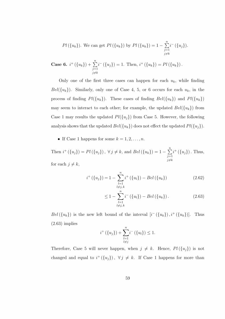
Pl (uk). We can get Pl (uk) by Pl (uk) = 1−n∑

j=1

j 6=k

i− (uj).


j=1

j 6=k

i− (uj) = 1. Then, i+ (uk) = Pl (uk) .

Only one of the first three cases can happen for each uk, while finding

Bel(uk). Similarly, only one of Case 4, 5, or 6 occurs for each uk, in the

process of finding Pl(uk). These cases of finding Bel(uk) and Pl(uk)

may seem to interact to each other; for example, the updated Bel(uk) from

Case 1 may results the updated Pl(uj) from Case 5. However, the following

analysis shows that the updated Bel(uk) does not effect the updated Pl(uj).

• If Case 1 happens for some k = 1, 2, . . . , n.

Then i+ (uj) = Pl (uj) , ∀ j 6= k, and Bel (uk) = 1−n∑

j=1

j 6=k

i+ (uj) . Thus,

for each j 6= k,

i+ (uj) = 1−n∑

l=1l 6=j, k

i+ (ul)−Bel (uk) (2.62)

≤ 1−n∑

l=1l 6=j, k

i− (ul)−Bel (uk) . (2.63)

Bel (uk) is the new left bound of the interval [i− (uk) , i+ (uk)]. Thus

(2.63) implies

i+ (uj) +n∑

l=1l 6=j

i− (ul) ≤ 1.

Therefore, Case 5 will never happen, when j 6= k. Hence, Pl (uj) is not

changed and equal to i+ (uj) , ∀ j 6= k. If Case 1 happens for more than

59

one k, says k1 and k2, we can set j := k1 and k := k2 (and vice versa) in

(2.62 - 2.63). Hence, Case 5 will never happen for any k = 1, 2, . . . , n, and

Pl (uk) = i+ (uk). However, if Case 1 happens for only one k, then Case 5

might happen for uk.

1. If Case 5 happens for uk, then Pl (uk) = 1−n∑

j=1

j 6=k

i− (uj). Moreover, for

each j 6= k,i− (uj) = 1−

n∑

l=1l 6=j, k

i− (ul)− Pl (uk) (2.64)

≥ 1−n∑

l=1l 6=j, k

i+ (ul)− Pl (uk) , (2.65)

which falls into Case 2 ,or 3. These two cases imply that Bel (uj) =

i− (uj) , ∀ j 6= k. Therefore, we obtain the tightest subinterval

[Bel(uk), P l(uk)] , ∀ k = 1, 2, . . . , n.

2. If Case 5 does not happen for uk, then Pl (uk) = i+ (uk). We still do

not know Bel (uj) , j 6= k. The case i− (uj)+n∑

l=1l 6=j

i+ (ul) < 1, ∃ j 6= k

will never happen, since we are considering when Case 1 happens just for

k. Hence, Bel (uj) = i− (uj) , ∀ j 6= k. We also obtain the tightest

subinterval [Bel(uk), P l(uk)] , ∀ k = 1, 2, . . . , n.

• If Case 1 has never happened for uk, ∀ k = 1, 2, . . . , n.

Then Bel (uk) = i− (uk) , ∀ k. If Case 5 also has never happened, then

Pl (uk) = i+ (uk) , ∀ k. If Case 5 happens for some k = 1, 2, . . . , n, then

Pl (uk) = 1 −n∑

j=1

j 6=k

i− (uj) and Pl (uj) = i+ (uj) , ∀ j 6= k. Moreover

(2.64) and (2.65) are true for these k. Suppose that there is more than one

60

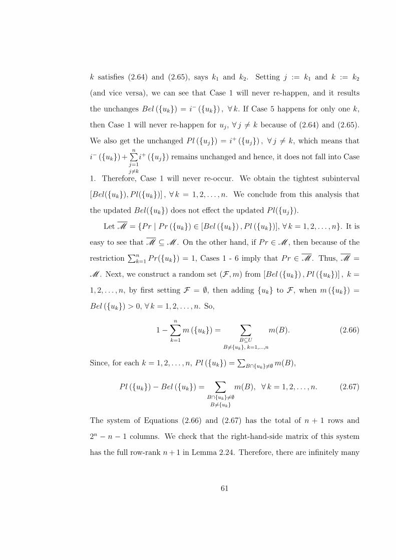
k satisfies (2.64) and (2.65), says k1 and k2. Setting j := k1 and k := k2

(and vice versa), we can see that Case 1 will never re-happen, and it results

the unchanges Bel (uk) = i− (uk) , ∀ k. If Case 5 happens for only one k,

then Case 1 will never re-happen for uj, ∀ j 6= k because of (2.64) and (2.65).

We also get the unchanged Pl (uj) = i+ (uj) , ∀ j 6= k, which means that

i− (uk)+n∑

j=1

j 6=k

i+ (uj) remains unchanged and hence, it does not fall into Case

1. Therefore, Case 1 will never re-occur. We obtain the tightest subinterval

[Bel(uk), P l(uk)] , ∀ k = 1, 2, . . . , n. We conclude from this analysis that

the updated Bel(uk) does not effect the updated Pl(uj).

Let M = Pr | Pr (uk) ∈ [Bel (uk) , P l (uk)], ∀ k = 1, 2, . . . , n. It is

easy to see that M ⊆M . On the other hand, if Pr ∈M , then because of the

restriction∑n

k=1 Pr(uk) = 1, Cases 1 - 6 imply that Pr ∈ M . Thus, M =

M . Next, we construct a random set (F ,m) from [Bel (uk) , P l (uk)] , k =

1, 2, . . . , n, by first setting F = ∅, then adding uk to F , when m (uk) =

Bel (uk) > 0, ∀ k = 1, 2, . . . , n. So,

1−n∑

k=1

m (uk) =∑

B⊆U

B 6=uk, k=1,...,n

m(B). (2.66)

Since, for each k = 1, 2, . . . , n, Pl (uk) =∑

B∩uk6=∅ m(B),

Pl (uk)−Bel (uk) =∑

B∩uk6=∅

B 6=uk

m(B), ∀ k = 1, 2, . . . , n. (2.67)

The system of Equations (2.66) and (2.67) has the total of n + 1 rows and

2n − n − 1 columns. We check that the right-hand-side matrix of this system

has the full row-rank n + 1 in Lemma 2.24. Therefore, there are infinitely many

61

solutions to 2n− n− 1 terms of m(B). We can construct one of the solutions of

the system as follows.

1. Set M := m(X) = min Pl (uk)−Bel (uk) , k = 1, 2, . . . , n. If M ≥

1−∑n

k=1 m (uk), set m(U) = 1−∑n

k=1 m (uk), and m(B) = 0, ∀B ⊆

U, B 6= U, B 6= uk , k = 1, 2, . . . , n, then we are done. Otherwise, let

Λ = 1, 2, . . . , n and Λ1 = k |M = Pl (uk)−Bel (uk). We have

m(B) = 0; ∀B ⊆ U, B 6= U, B ∩ uk 6= ∅, and B 6= uk , ∀ k ∈ Λ1.

2. Now, we consider the system (2.67) when k ∈ Λ − Λ1. Choose an

unknow value m(B1) for some B1 ⊆ U , such that m(B1) is a term

in∑

B∩uk6=∅

B 6=uk

m(B), for each k ∈ Λ − Λ1. Such a set B1 always ex-

ists. Set m(B1) = min Pl (uk)−Bel (uk)−M, ∀ k ∈ Λ− Λ1. If

m(B1) ≥ 1 −∑n

k=1 m (uk)−M , set m(B1) = 1−∑n

k=1 m (uk)−M ,

and m(B) = 0 for the rest of unassigned value m(B)’s, then we are

done. Otherwise, set M := m(B1), and Λ2 := k |M = Pl (uk)−

Bel (uk). Again, we have m(B) = 0 for every unassigned value m(B)

in∑

B∩uk6=∅

B 6=uk

m(B), k ∈ Λ2.

3. Set Λ1 := Λ1 ∪ Λ2, return to step 2.

We add set B ⊆ U into F , whenever m(B) > 0. Hence, we obtain a random

set (F ,m). The procedure of constructing this random set will terminate in a

finite number of iterations, since U is finite. It is indeed a random set, since

∑A∈F m(A) = 1.

Lemma 2.24 The system of Equations (2.66 - 2.67) has the full row-rank.

62

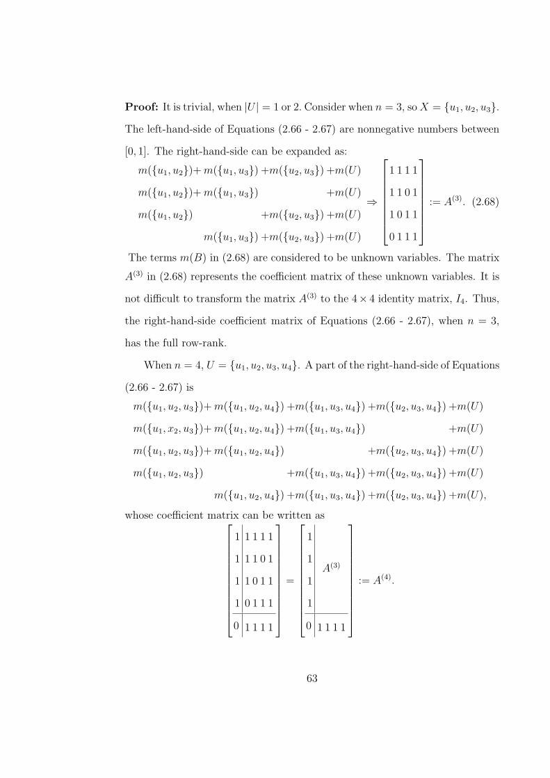
Proof: It is trivial, when |U | = 1 or 2. Consider when n = 3, so X = u1, u2, u3.

The left-hand-side of Equations (2.66 - 2.67) are nonnegative numbers between

[0, 1]. The right-hand-side can be expanded as:

m(u1, u2)+ m(u1, u3) +m(u2, u3) +m(U)

m(u1, u2)+ m(u1, u3) +m(U)

m(u1, u2) +m(u2, u3) +m(U)

m(u1, u3) +m(u2, u3) +m(U)

⇒

1 1 1 1

1 1 0 1

1 0 1 1

0 1 1 1

:= A(3). (2.68)

The terms m(B) in (2.68) are considered to be unknown variables. The matrix

A(3) in (2.68) represents the coefficient matrix of these unknown variables. It is

not difficult to transform the matrix A(3) to the 4× 4 identity matrix, I4. Thus,

the right-hand-side coefficient matrix of Equations (2.66 - 2.67), when n = 3,

has the full row-rank.

When n = 4, U = u1, u2, u3, u4. A part of the right-hand-side of Equations

(2.66 - 2.67) is

m(u1, u2, u3)+ m(u1, u2, u4) +m(u1, u3, u4) +m(u2, u3, u4) +m(U)

m(u1, x2, u3)+ m(u1, u2, u4) +m(u1, u3, u4) +m(U)

m(u1, u2, u3)+ m(u1, u2, u4) +m(u2, u3, u4) +m(U)

m(u1, u2, u3) +m(u1, u3, u4) +m(u2, u3, u4) +m(U)

m(u1, u2, u4) +m(u1, u3, u4) +m(u2, u3, u4) +m(U),

whose coefficient matrix can be written as

1

1

1

1

1 1 1 1

1 1 0 1

1 0 1 1

0 1 1 1

0 1 1 1 1

=

1

1

1

1

A(3)

0 1 1 1 1

:= A(4).

63

Again, we can transform A(4) to I5 by using the Gauss - Jordan elimination

method. Hence, the right-hand-side coefficient matrix of Equations (2.66 - 2.67),

when n = 4, has the full row-rank.

In general, for |X| = k = 4, 5, . . . , n − 1, we have U = u1, u2, . . . , uk.

A part of the right-hand-side of Equations (2.66 - 2.67) can be written as the

following square matrix of dimension (k + 1)× (k + 1), which associates with k

of unknown terms m(B), where |B| = k − 1, and m(U).

1

1

...

1

A(k−1)

0 1 1 · · · 1

:= A(k), ∀ k = 1, 2, . . . , n− 1.

By mathematical induction, suppose that A(k) can be transformed to the identity

matrix, I(k+1), for each k = 1, 2, . . . , n− 1. Thus, for k = n, the matrix

1

1

...

1

A(n−1)

0 1 1 · · · 1

:= A(n)

can be transformed to I(n+1) by Gauss - Jordan elimination. Hence, the right-

hand-side coefficient matrix of Equations (2.66 - 2.67) has the full row-rank,

when |U | = 3, 4, . . . , n.

Lemma 2.23 helps transform probability interval information to (not unique)

random set information. However, we may not get two probability density

64

mass functions from this random set to obtain the largest bound on the ex-

pected value of u. To guarantee the smallest and the largest expected val-

ues of u given probability intervals information, we solve the LP problems:

minf

/ maxf

Ef (u) s.t. f(ui) ∈ [ai, ai],n∑

i=1

f(ui) = 1, and f(ui) ≥ 0, ∀ i.

Let A = A1, A2, . . . , Ai ⊆ P(U), for some i ∈ N, i ≤ 2|U | − 1. Sup-

pose we know the values of probabilities on these sets in A, Pr(Ak) = pk,

k = 1, 2, . . . , i, but the information is not enough to provide the values of

Pr(uk),∀ k. Then, we may not be able to find any random set to repre-

sent probability on sets information, because MA 6= M, in general, where

MA = Pr : Pr(Ak) = pk, ∀Ak ∈ A, and M is the set of probability gen-

erated by a random set. Therefore, a probability on sets interpretation of an

uncertainty u is not a special case of a random set interpretation. It can be an

example of an IVPM by setting

i(A) =

[Pr(A), P r(A)] ; A ∈ A,

[0, 1] ; A ∈ P(U)\A.(2.69)

To guarantee the smallest and the largest expected values of u given a probability

on sets information, we solve the LP problems:

minf

/ maxf

Ef (u) s.t.∑

ui∈Ak

f(ui) = pk, ∀Ak ∈ A, andn∑

i=1

f(ui) = 1.

Let Bel(Ak) = αk, and Pl(Ak) = βk, ∀Ak ∈ A. Suppose we have partial

information in the form of belief (or plausibility) of some subsets of U , then for

an unknown probability Pr that obeys this partial information, αk = Bel(Ak) ≤∑

ui∈AkPr(ui), ∀Ak ∈ A, (or βk = Pl(Ak) ≥

∑ui∈Ak

Pr(ui), ∀Ak ∈ A). We

65

can write belief of some subsets of U as the following IVPM:

i(A) =

[Bel(A), 1] ; A ∈ A,

[0, 1] ; A ∈ P(U)\A.(2.70)

To guarantee the smallest and the largest expected values of u given a probability

on sets information, we solve the LP problems:

minf

/ maxf

Ef (u) s.t.∑

ui∈Ak

f(ui) ≥ αk, ∀Ak ∈ A, andn∑

i=1

f(ui) = 1.

A similar approach applies to a partial information of plausibility on subsets of

the set U .2.3.1 Upper and lower expected values generated by IVPMs

We consider the case when the incomplete information is interpreted as

an IVPM, i.e., suppose that a finite set U of n realizations of u is defined by

U := u1, u2, . . . , un, where u1 ≤ u2 ≤ . . . ≤ un, and have the probability

information in a nonempty set P as follows:

P =

(Pr1, P r2, . . . , P rn)

∣∣∣∣∣∣∣∣∣

ai ≤∑

k∈Λi

Prk ≤ ai, ∀i = 1, 2, . . . , t,

n∑

k=1

Prk = 1, P rk ≥ 0, ∀k = 1, 2, . . . , n.

(2.71)

Λi in (2.71) is an index set which is a subset of 1, 2, . . . , n, where t is

the total number of index sets, i.e., t ∈ N and t ≤ 2n − 2. The unknown

probability of uk is Prk. The sum of these probabilities in Λi is λi ∈ [0, 1].

Let Pr be any probability satisfying (2.71), and EPr(u) denote the expected

values of u, with respect to Pr. We show in Theorem 2.25 and Corollary 2.26

below that there are density mass functions Pr∗ and Pr∗ such that the expected

value of u with respect to Pr∗ and Pr∗ are the lower and the upper bounds on

all expected values of u with respect to any probability satisfies (2.71), i.e.,

EPr∗(u) ≤ EPr(u) ≤ EPr∗(u).

66

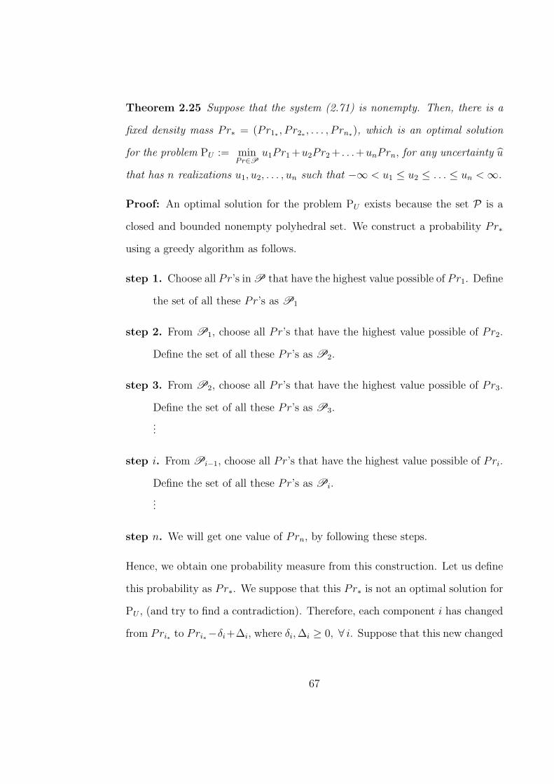
Theorem 2.25 Suppose that the system (2.71) is nonempty. Then, there is a

fixed density mass Pr∗ = (Pr1∗ , P r2∗ , . . . , P rn∗), which is an optimal solution

for the problem PU := minPr∈P

u1Pr1 +u2Pr2 + . . .+unPrn, for any uncertainty u

that has n realizations u1, u2, . . . , un such that −∞ < u1 ≤ u2 ≤ . . . ≤ un <∞.

Proof: An optimal solution for the problem PU exists because the set P is a

closed and bounded nonempty polyhedral set. We construct a probability Pr∗

using a greedy algorithm as follows.

step 1. Choose all Pr’s in P that have the highest value possible of Pr1. Define

the set of all these Pr’s as P1

step 2. From P1, choose all Pr’s that have the highest value possible of Pr2.

Define the set of all these Pr’s as P2.

step 3. From P2, choose all Pr’s that have the highest value possible of Pr3.

Define the set of all these Pr’s as P3.

...

step i. From Pi−1, choose all Pr’s that have the highest value possible of Pri.

Define the set of all these Pr’s as Pi.

...

step n. We will get one value of Prn, by following these steps.

Hence, we obtain one probability measure from this construction. Let us define

this probability as Pr∗. We suppose that this Pr∗ is not an optimal solution for

PU , (and try to find a contradiction). Therefore, each component i has changed

from Pri∗ to Pri∗−δi+∆i, where δi, ∆i ≥ 0, ∀ i. Suppose that this new changed

67

probability is optimal for PU . Let Z be the minimal objective value of PU . This

requires the analysis of n cases.

Case 1. Suppose that Pr1∗ changes to Pr1∗ − δ1 + ∆1.

We know that some other components i, i 6= 1, also need to be changed, so that

this changed probability still satisfies the conditions in P. The 1st component

can only be reduced, i.e., Pr1∗ − δ1, for some δ1 > 0, since Pr1∗ is the highest

value by the construction above. Thus,

Z = u1 (Pr1∗ − δ1) + u2 (Pr2∗ − δ2 + ∆2) + u3 (Pr3∗ − δ3 + ∆3) + . . . +

un (Prn∗ − δn + ∆n) .

As we know that Pr1∗ − δ1 can be increased, let us increase it by λ1, where

0 < λ1 ≤ δ1, and to be able to satisfy P, Pri∗ − δi + ∆i may be reduced by

λi ≥ 0, such that∑n

i=2 λi = λ1. Hence,

Z1 = u1 (Pr1∗ − δ1 + λ1) + u2 (Pr2∗ − δ2 + ∆2 − λ2) + u3 (Pr3∗ − δ3 + ∆3 − λ3)

+ . . . + un (Prn∗ − δn + ∆n − λn)

= u1 (Pr1∗ − δ1) + u2 (Pr2∗ − δ2 + ∆2) + u3 (Pr3∗ − δ3 + ∆3) + . . . +

un (Prn∗ − δn + ∆n) + (u1 − u2)λ2 + (u1 − u3)λ3 + . . . + (u1 − un)λn

= Z + (u1 − u2)λ2 + (u1 − u3)λ3 + . . . + (u1 − un)λn.

Now, consider Θ = (u1−u2)λ2+(u1−u3)λ3+. . .+(u1−un)λn. If u1 < u2 < . . . <

un, then Θ < 0. Hence, Z1 < Z. If ui = ui+1 = ui+2 = . . . = ui+j = u, for some

i ≥ 1 and i+ j ≤ n, then Θ = (u1−u2)λ2 +(u1−u3)λ3 + . . .+(u1−ui−1)λi−1 +

(u1− (j− i+1)u)(λi +λi+1 + . . .+λj)+ (ui−uj+1)λj+1 + . . .+(u1−un)λn < 0.

Hence, Z1 < Z.

68

Case 2. Suppose that Pr2∗ changes to Pr2∗ − δ2 + ∆2, where ∆2 − δ2 6= 0.

We know that some other components i, i 6= 2, also need to be changed, so that

this changed probability still satisfies the conditions in P. The 1st component

can only be reduced, i.e., Pr1∗ − δ1, for some δ1 > 0, since Pr1∗ is the highest

value by the construction above. If Pr1∗ is reduced, then it becomes the previous

case. If there are no changes in Pr1∗ , then this changed probability is in P1.

Pr2∗ can only be decreased, otherwise this changed probability is not in P1.

So, Pr2∗ changes to Pr2∗ − δ2, for some δ2 > 0. Thus,

Z = u1 (Pr1∗) + u2 (Pr2∗ − δ2) + u3 (Pr3∗ − δ3 + ∆3) + . . . + un (Prn∗ − δn + ∆n) .

By a similar pattern as in Case 1, we know that Pr2∗ − δ2 can be increased.

Let us increase it by λ2, where 0 < λ2 ≤ δ2, and to be able to satisfy P,

Pri∗ − δi + ∆i may be reduced by λi ≥ 0, such thatn∑

i=3

λi = λ2. Hence,

Z2 = u1 (Pr1∗) + u2 (Pr2∗ − δ2 + λ2) + u3 (Pr3∗ − δ3 + ∆3 − λ3)

+ . . . + un (Prn∗ − δn + ∆n − λn)

= u1 (Pr1∗) + u2 (Pr2∗ − δ2) + u3 (Pr3∗ − δ3 + ∆3) + . . . +

un (Prn∗ − δn + ∆n) + (u2 − u3)λ3 + (u2 − u4)λ4 + . . . + (u2 − un)λn

= Z + (u2 − u3)λ3 + (u2 − u3)λ4 + . . . + (u2 − un)λn.

Hence, Z2 < Z. We apply a similar argument to the rest of the cases. Then,

the changed probability is not optimal, a contradiction. Thus, Pr∗ is an optimal

solution for PU .

69

Corollary 2.26 Suppose that the system (2.71) is nonempty. Then, there is

a fixed density mass Pr∗ = (Pr∗1, P r∗2, . . . , P r∗n) as an optimal solution for the

problem PV := maxPr∈P

v1Pr1 + v2Pr2 + . . . + vnPrn, for any uncertainty v that

has n realizations v1, v2, . . . , vn such that −∞ < v1 ≤ v2 ≤ . . . ≤ vn <∞.

Proof: Apply Theorem 2.26 by using v1 = −un, v2 = −un−1, . . . , and vn =

−u1.

Next, the concept of clouds is presented. We point out some differences

between clouds and IVPMs and give an example to shows that a cloud could be

represented as an IVPM.

2.4 Clouds

The concept of a cloud, which tries to combine probability and possibility

into one conceptual basis, was introduced by Neumaier in [52]. The general

definition of a cloud is given below.

Definition 2.27 (see Neumaier, [52]) Suppose all realizations of an uncertainty

parameter are in a set U . A cloud over set U is an interval mapping c : U →

Int[0,1] such that

1. ∀u ∈ U ; c(u) = [c(u), c(u)] with c(u), c(u) ∈ R, 0 ≤ c(u) ≤ c(u) ≤ 1, and

2. (0, 1) ⊆⋃

u∈U

c(u) ⊆ [0, 1].

In addition, a random variable Y taking values in U is said to belong to cloud

c, (written as Y ∈ c), if and only if

∀α ∈ [0, 1]; Pr(c(Y ) ≥ α) ≤ 1− α ≤ Pr(c(Y ) > α). (2.72)

70

There is at least one random variable belonging to any given cloud. The

proof of this statement is given in [51]. This random variable is proved to exist,

not assumed to exist as in the definition of an IVPM. We can restate the property

(2.72) by saying that

• the probability that a random variable Y ∈ c belongs to the upper α-cut

Aα := u ∈ U | c(u) > α is at least 1− α, and

• the probability that a random variable X ∈ c belongs to the lower α-cut

Aα := u ∈ U | c(u) ≥ α is at most 1− α.

Figure 2.5 shows a cloud over R with an α-cut.

α = 0.6

Aα

Aα

1

x

c(x)

Figure 2.5: A cloud on R with an α-cut at α = 0.6.

Definition 2.28 (see Jamison [24]) Let pos : U → [0, 1] be a regular possibil-

ity distribution function, i.e., supu

pos(u) ∈ U = 1, with associated possibility

measure Pos and necessity measure Nec, (no need to be the dual of Pos). Then

pos is said to be consistent with a random variable Y if for every measurable

set A, Nec(A) ≤ Pr(Y ∈ A) ≤ Pos(A).

A pair of necessity and possibility measures in Definition 2.28 is an example

of an IVPM. The reference [36] shows that every cloud c can be defined as

c(u) = [n(u), p(u)], where p and p are regular possibility distribution functions

71

Table 2.3: The differences between IVPMs and clouds

IVPMs Clouds

Domain σX X

Range i(A) = [i−(A), i+(A)] ⊆ [0, 1], c(x) = [c(x), c(x)],∀x ∈ X, and

∀A ∈ σX (0, 1) ⊆⋃

x∈X

c(x) ⊆ [0, 1]

Random assumed to a part proved to be

variable of IVPM’s definition in any clouds

Example [Nec(A), Pos(A)] [nec(x), pos(x)], when pos is

regular possibility distribution

on X such that ∀u ∈ U ; p(u)+p(u) ≥ 1 and n(u) = 1−p(u), and their associated

possibility measures are consistent with every random variable belonging to c.

More specifically, Destercke et al., [11] , proves that a cloud c is representable by

the pair of possibility distributions 1− c and c. We distinguish some differences

between the definitions of an IVPM and a cloud in Table 2.3.

Example 11. Suppose U = 1, 2, 3, 4, 5, 6. A cloud over set U is given in

Figure 2.6. We can see that

1

0.5

0.1

0.8

1 2 3 4 5 6

: c: c

Figure 2.6: A cloud represents an IVPM.

72

α = 0⇒ Pr (U) ≤ 1− 0 ≤ Pr (U) ,

α ∈ (0, 0.1)⇒ Pr (2, 3, 4, 5) ≤ 1− α ≤ Pr (U) ,

α = 0.1⇒ Pr (2, 3, 4, 5) ≤ 1− 0.1 ≤ Pr (2, 3, 4, 5) ,

α ∈ (0.1, 0.5)⇒ Pr (3) ≤ 1− α ≤ Pr (2, 3, 4, 5) ,

α = 0.5⇒ Pr (3) ≤ 1− 0.5 ≤ Pr (3, 4) ,

α ∈ (0.5, 0.8]⇒ Pr (3) ≤ 1− α ≤ Pr (3, 4) ,

α ∈ (0.8, 1)⇒ 1− α ≤ Pr (3, 4) .

Hence, Pr(U) = 1, Pr (2, 3, 4, 5) = 0.9, Pr (1, 6) = 0.1, Pr (3) ≤ 0.2,

and Pr (3, 4) ≥ 0.2. This information can be considered as an IVPM, because

we can set i (3) = [0, 0.2], i (3, 4) = [0.2, 1], and i(A) = [0, 1], whenever any

nonempty subset A of U is not one of the sets U, 2, 3, 4, 5 , 1, 6 , 3, 4, or

3. ♦

Any cloud can be represented as an IVPM, in general. Hence, we conclude

that clouds are special examples of IVPMs. Walley [73] introduced his imprecise

probability theories to characterize a set of gambles of interest, where a gamble

is a bounded real-valued function defined on a set U . However, his approach is

too general for uncertainties concerned in this dissertation. We will not present

the details of Walley’s imprecise probability in this thesis. Interested readers

can find out more in [73]. A discussion of relationships of these concepts in the

sense of theory ‘A’ is more general than theory ‘B’ is well explained in [10] and

[11]. We are interesting in arguing the relationships of different interpretations

of an uncertainty u. These interpretations are

1. possibility measure

73

(a) possibility distribution

(b) possibility on some subsets of U

2. necessity measure

(a) necessity distribution

(b) necessity on some subsets of U

3. plausibility measure

(a) plausibility distribution

(b) plausibility on some subsets of U

4. belief measure

(a) belief distribution

(b) belief on some subsets of U

5. random set

6. probability interval

7. probability on sets

8. cloud

9. IVPM.

We wish to use an appropriate approach to obtain two special probability density

mass functions that provide the smallest and the largest expected values of u.

74

2.5 Relationships of some selected uncertainty interpretations

Some results in this chapter are generalized to be able to handle the continu-

ous case of U . However for simplicity, we reduce the scope of this dissertation to

the finite case of U . Since an interval interpretation of uncertainty falls into the

continuous case of U , we will not consider interval uncertainty in this research.

The continuous case is for further research.

We summarize the review of the interpretations of an uncertainty from Sec-

tions 2.1 - 2.4 as follows.

• We can derive a unique random set from possibility, necessity, plausibility,

or belief measures by using the formula (2.10).

• We can derive a unique possibility, necessity, plausibility, or belief measures

by using the formula (2.7) or (2.8).

• We can generate the random set that provides the largest set MF from

a given partial information of a random set, as explained in Subsection

2.2.2.

• We can generate the random set that provides the largest set MF from

a given a possibility, a necessity, a plausibility, or a belief distribution, as

explained in Subsections 2.2.3 - 2.2.6.

• There is the random set generated by partial information in the form of

possibility or necessity on some subsets of U . This random set also provides

the largest setMF .

• We can construct a random set from a given probability interval.

75

• Random set, probability interval, probability on sets, and cloud are exam-

ples of IVPMs.

• We consider partial information in the form of belief or plausibility on

some subsets of U as an IVPM information.

• Probability is just a random set when all focal elements are singletons.

We now provide a full relationship diagram of all different uncertainty interpre-

tations related to this thesis in Figure 2.7, which enhances the basic diagram of

Figure 1.1 in Chaper 1.

We will never know with certainty the probability of a parameter when

information we received is one of the uncertainty interpretations mentioned in

this chapter. However, we can at least find out two probability density mass

functions from M that provide the smallest and the largest expected values.

There are two approaches to obtain these two probability density mass functions.

The first approach is by the constructions (2.42) and (2.43) when an uncertainty

interpretation can be viewed as a random set. The second approach is by setting

up two associated LP problems to solve for the minimum and maximum expected

values of u, when an uncertainty interpretation is considered to be an IVPM.

Our contribution results in this chapter are summarized below.

1. Remarks 2.9 and 2.10 provide the insight that Bel(A) and Pl(A), for each

A ⊆ U , depend on the set Ω. Moreover, if we receive more informa-

tion where the old information becomes more specific, then Belold(A)) ≤

Belupdated(A)) ≤ Plupdated(A)) ≤ Plold(A)).

76

Possibilitydistribution

orPossibility

on sets

Necessitydistribution

orNecessityon sets

Plausibilitydistribution

orBelief

distribution

Belief orPlausibility

on sets

Random set

Subsection2.2.3

Subsection

2.2.4

Subse

ctio

ns

2.2.

5,2.

2.6

Probabilitymeasure singleton focal

elements

Probabilityinterval

Lemma 2.2

3

IVPM

Probabilityon sets

Equatio

n(2

.70)

[Bel(A), P l(A)]

Cloud

Beliefmeasure

Plausibilitymeasure

.

Pl(A) = 1 − Bel(AC)

m(A) =∑

B⊆A

(−1)|A\B|Bel(B)

Bel(A) =∑

B⊆A

m(B)

Necessitymeasure

Possibilitymeasure

Pos(A) = 1 − Nec(AC) . .nestedfocal

elements

Equation

(2.60)

Equatio

n(2

.69)E

quat

ion

(2.72)

Figure 2.7: Uncertainty interpretations: A −−→ B : there is an uncertaintyinterpretation B contains information given by an uncertainty interpretation A,A −−→ B : A is a special case of B, A ←→ B : A and B can be derived fromeach other, and A · · · → B : B generalized A.

77

2. We provide a stronger statement to ensure the meanings of possibility and

necessity, i.e., Nec(A ∩ B) = min Nec(A), Nec(B) and Pos(A ∪ B) =

max Pos(A), Pos(B) if and only if the focal elements are nested. The

proof of this statement is in Appendix B.

3. Based on a given uncertainty u with random set interpretation, we prove

in Theorem 2.15 that the lower and upper functions of M are belief and

plausibility functions.

4. Theorem 2.17 and 2.18 guarantee that probability density functions f and

f provide the lowest and the highest expected values for a given uncertainty

u with random set interpretation. For a finite set of realizations of u, Table

2.2 illustrates the number of Bel and Pl terms needed to derive f and f ,

which is much less than the number of Bel and Pl terms needed to state

LP problems to find the lowest and the highest expected values.

5. Subsections 2.2.2 - 2.2.6 emphasize that if we have only partial information

about belief (or other) measure or random set, then we still can find the

random set generated by this partial information that provides the largest

setMF .

6. We can find a (not unique) random set that contains information given by

a probability interval, see Lemma 2.23.

7. Theorem 2.25 and Corollary 2.26 are used for finding f and f , when u has

IVPM interpretation.

78

8. We provide the relationships of PC-BRIN interpretations of uncertainty

in Figure 2.7.

Chapter 4 explains how to solve an LP problem with uncertainty to get

a pessimistic and an optimistic result. It involves using these two probability

density mass functions and two expected recourse models. Moreover, a minimax

regret approach for an LP problem with uncertainty is presented to provide a

minimax regret solution when the true probability of uncertainty is unknown,

but its bound is known. The next chapter is devoted to a literature review of

linear programming problems with uncertainty. Uncertainty presented in the

review is limited to probability measure, possibility distribution, and interval

(which is not developed in this thesis).

79

3. Linear optimization under uncertainty: literature review

We provide a review of literature dealing with modeling LP problems with

uncertainty. If the objective is to find a solution for an LP problem with un-

certainty that will minimize the maximum regret of using this solution due to

the uncertainty, we may apply a minimax regret model to the problem and

ignore any interpretations of uncertainty. However, if we are interesting in pre-

dicting the average of objective values in the long run, then we must consider

uncertainty interpretations. Toward this end, we categorize uncertainty in LP

problems depending on the information available about the uncertainties. They

fall into the following cases.

• Uncertainty interpretations in the problem are probability. The modeling

approach is an expected recourse model.

• Uncertainty interpretations in the problem are possibility. The modeling

approach is an expected average model.

• Uncertainty interpretations in the problem can be both probability and

possibility, but they are not in the same constraint. The modeling ap-

proach is an expected recourse-average model.

• Uncertainty interpretations in the problem can be both probability and

possibility in the same constraint. The modeling approach is an interval

expected value model.

80

To date, there is no modeling concept that capture LP problems with other

uncertainty interpretations, except the ones listed above. We try to overcome

this disadvantage by using a new approach (based on an expected recourse

model), which uses the knowledge we had from Chapter 2 that each of PC-BRIN

uncertainty can be represented as a set of all probability measures associated

with their information. The details of the new approach are provided in Chapter

4.

In this chapter, the modeling concepts for the LP problems with uncertainty

categorized above are presented. We begin with an illustration of a deterministic

model of a production planning example. Then, after we explain the modeling

concept for each of the LP problems with uncertainty categorized above, we

provide an example for each concept by modifying this production planning

example, which leads us to different types of models depending on the inter-

pretations of uncertainties. The solutions of these models are done in GAMS,

which is a program language for solving general optimization problems. For

simplicity, we assume that we have information that already has been classified

into probability and possibility interpretations of uncertainty. The differences

should be seen in modeling and semantics of each example.

3.1 Deterministic model

A small production scheduling example is presented for ease and clarity of

presentation. From two raw materials x1 and x2, (for example, supplies of two

grades of mineral oil), a refinery produces two different goods, cream #1 and

cream #2. Table 3.1 shows the output of products per unit of the raw materials,

the unit costs of raw materials (yielding the production cost z), the demands

81

for the products, and the maximal total amount of raw materials (production

capacity) that can be processed. We assume that the mineral oil is mixed with

other fluids (e.g., water) at no production cost to manufacture. Hence, these

ingredients are not in the model.

Table 3.1: Productivity information shows the output of products per unit ofraw materials, the unit costs of raw materials, the demand for the products, andthe limitation of the total amount of raw materials.

Mineral oil Products Costs The limit amount of(fl.oz.) cream #1 cream #2 ($/fl.oz.) mineral oil that

(oz./fl.oz.) (oz./fl.oz.) can be processed (fl.oz.)x1 2 3 2 1x2 6.1667 3 3 1

relation ≥ ≥ = ≤Demands

174.83 161.75 z 100

A manager wants to know how many units of raw materials to order to

satisfy the demands and minimize the total production cost. Therefore, we

have the linear programming problem (3.1) with the unique optimal solution

(x∗1, x

∗2) = (37.84, 16.08), and z∗ = $123.92. Figure 3.1 illustrates the feasible

region of the system (3.1) and its unique optimal solution.

min z := 2x1 + 3x2

s.t. 2x1 + 6.1667x2 ≥ 174.83,

3x1 + 3x2 ≥ 161.75,

x1 + x2 ≤ 100,

x1, x2 ≥ 0.

(3.1)

The values shown in Table 3.1 are fixed for the deterministic problem (3.1).

However, this is not always a realistic assumption. For instance, if the produc-

82

x2

x1

3x1 + 3x2 = 161.75

2x1 + 6.1667x2 = 174.83

x1 + x2 = 100

x∗2 = 16.08

x∗1 = 37.84

z∗ = 123.92

z = 200z = 270

Figure 3.1: Feasible region and the unique optimal solution of the productionscheduling problem (3.1).

tivities and demands can vary within certain limits or even have different types

of uncertainty, and/or we need to formulate a production plan before knowing

the exact values of these data, then this deterministic model is not adequate.

We have to reformulate the system (3.1) so that it can produce a reasonable re-

sult. In Sections 3.2-3.6, we present different types of models depending on the

interpretations of uncertainty to put the main thrust of this thesis, pessimistic,

optimistic and minimax regret of expected recourse problems, in the context of

other optimization under uncertainty.

3.2 Stochastic models

The aim of stochastic programming is to find an optimal decision in problems

involving uncertain data of probability interpretation. The terminology ‘stochas-

tic’ is opposed to ‘deterministic’ and means that some data are random. There

are two well-known stochastic programming models. One is a stochastic program

with expected recourse, which transforms the randomness contained in a stochas-

tic program into an expectation of the distribution of some random vector. The

83

other is a stochastic program with chance constraints, which the constraints can

satisfy the requirements with some probability or reliability level. One of these

models is chosen for a particular problem under appropriate assumptions. How-

ever, we will not present a stochastic program with chance constraints in this

dissertation. The details on this topic can be found in many books , e.g., [5, 26].

A general formulation for a stochastic linear program is the same as the

model (1.2), when A and b have probability interpretations. We restate this

problem here:

minx

cTx s.t. Ax ≥ b, Bx ≥ d, x ≥ 0, (3.2)

where Ax ≥ b contains m constraints of uncertain inequalities. This problem is

not well-defined, because of the uncertainties. To be more specific, let us assume

the following in addition to what we had in the problem (3.1).

A1 The raw materials for the weekly production process rely on the supply of

two grades of mineral oil, denoted by x1 and x2, respectively.

A2 The refinery uses two grades of mineral oil (and other ingredients at no

cost) to produce cream #1 and cream #2.

A3 The weekly demands of cream #1 and cream #2 vary randomly and mu-

tually independent on each other (for simplicity).

A4 The production (the output of the product per unit of the raw materials)

of cream #1 varies randomly.

A5 The production per unit of cream #2 is fixed.

84

Given the above assumptions, the problem becomes a stochastic linear program

(3.3), where a11 and a12 are the production of cream #1 per unit of mineral oil x1

and x2, and b1 and b2 are random demands. They possess known probability of

demands for cream #1 and cream #2, respectively. It is not clear how to solve

the minimization problem (3.3), since it is not a well-defined problem before

knowing the realizations of (a11, a12, b1, b2).

min 2x1 + 3x2

s.t. a11x1 + a12x2 ≥ b1, 3x1 + 3x2 ≥ b2,

x1 + x2 ≤ 100, x1, x2 ≥ 0.

(3.3)

We have to formulate a production plan under uncertainty, since we only have

the probability distributions of the random demands.

3.2.1 Stochastic program with expected recourse

The terminology ‘recourse’ refers to a second (or further) action that helps

improve a situation whenever the first action (taken before knowing the real-

ization of uncertainty) does not satisfy the requirements. An example of the

situation and requirements in the model is when the manufacturer is required to

satisfy the customer’s demands, which are uncertain, while trying to minimize

the production cost. The manager has to make a decision on the amount of raw

materials (the first action) without knowing the actual demands. Later on, if

these amounts of raw materials do not satisfy the actual demands, the manager

needs to buy any shortage amount (recourse variables, or second action) from

an outside market with some price attached.

An expected recourse model minimizes the cost of the first action and

the expected cost of the second action. Define the random vector ξ =

85

(a11, a12, . . . , amn, b1, b2, . . . , bm)T, and the penalty price vector for m constraints

as s = (s1, s2, . . . , sm)T ≥ 0. Let Ψ = x | Bx ≥ d, x ≥ 0. An expected re-

course model has the general formula

minx∈Ψ

cTx + Eξ Q(x, ξ), (3.4)

where Eξ Q(x, ξ) is the expected value of Q(x, ξ) with respected to random vari-

able ξ, and Q(x, ξ) = sT(max

[(b− Ax), 0

]). More precisely, suppose there are

αij and βi finite realizations of each uncertainty aij in the matrix A and bi in the

vector b, respectively. Thus, there are Πnj=1Π

mi=1αijβi = N scenarios of ξ, which

are denoted as ξk, ∀ k = 1, 2, . . . , N . Each scenario has probability of occurrence

prk. Hence, Q(x, ξ) =(Q(x, ξ1), Q(x, ξ2), . . . , Q(x, ξN )

), where Ak and bk are the

matrix and vector at the kth scenario, and Q(x, ξk) = sT(max

[(bk − Akx), 0

]).

Let y(ξ) = max[(b− Ax), 0

]. The variable y(ξ) is a recourse variable vector of

shortages. Model (3.4) can be rewritten as

minx∈Ψ

cTx + Eξ (sTy(ξ)) s.t. y(ξ) ≥ b− Ax, y(ξ) ≥ 0. (3.5)

We illustrate an example of an expected recourse problem by supposing that

the assumptions A1-A5 apply to this subsection and assume further as follows.

A6 Fixed amounts x1 and x2 of two grades of mineral oil must be chosen in

advance of knowing actual demand and cannot change during the week.

A7 The customers expect their actual demands of cream #1 and cream #2 to

be satisfied.

A8 Fixed ‘penalty ’ prices will be incurred if the customer’s demands cannot be

covered by the production, since the amount of shortages has to be bought

from a market.

86

We assume here that the penalty prices per unit of shortages are s1 = $7 and

s2 = $12 for cream #1 and cream #2, respectively. For simplicity, we suppose

further that there is no storage cost or selling cost for the over production.

Assume that the realizations of the random productivity of cream #1 and

the random demands of both creams are finite with their probabilities as follows:

a11 =

1 Pr (1) = 1/4

2 Pr (2) = 1/2

3 Pr (3) = 1/4

a12 =

5 Pr (5) = 1/6

6 Pr (6) = 1/2

7 Pr (7) = 1/3

b1 =

149 Pr (149) = 5/12

180 Pr (180) = 1/3

211 Pr (211) = 1/4

b2 =

138 Pr (138) = 1/4

162 Pr (162) = 1/2

185 Pr (185) = 1/4.

(3.6)

Define the random vector ξ =(a11, a12, b1, b2

)T

=ξ1 = (1, 5, 149, 138)T , ξ2 =

(1, 5, 149, 162)T , . . . , ξ81 = (3, 7, 211, 185)T, and introduce recourse variables

y1(ξ) and y2(ξ) measuring the shortages of cream #1 and cream #2, respec-

tively. The yi(ξ), i = 1, 2, are themselves random variables since shortage de-

pends on the realizations of random vector ξ. We also refer to the expected

costs due to any shortage of production (or due to the amount of violation in

the constraints, in general) as the expected recourse costs. We can replace the

stochastic problem (3.3) by the well-defined stochastic program with expected

recourse (3.7) using Eξ as an expected value with respect to the distribution of

ξ.

min 2x1 + 3x2 + Eξ Q (x1, x2, ξ)

s.t. x1 + x2 ≤ 100,

x1, x2 ≥ 0,

(3.7)

87

where for each j = 1, 2, . . . , 81,

Q(x1, x2, ξ

j)

:= 7 maxbj1 − aj

11x1 − aj12x2, 0

+ 12 max

bj2 − 3x1 − 3x2, 0

= min 7y1 + 12y2

s.t. aj11x1 + aj

12x2 + y1(ξj) ≥ bj

1,

3x1 + 3x2 + y2(ξj) ≥ bj

2,

y1, y2 ≥ 0.

The mathematical program (3.7) is a linear programming problem which yields

an optimal solution of x∗1 = 31.80 and x∗

2 = 29.87, with the corresponding

production (first-stage) costs of $153.21 and the sum of the first-stage costs

and the expected recourse costs of $155.38. This optimal solution violates x1 +

5x2 ≥ 211, which results in the recourse variable y1(ξ3) = 29.85. However, this

constraint happens with a very small probability of 14

16

14

= 196

. Hence, we can

interpret this optimal solution as that in the long run, the manufacturer will

spend on average of $153.21 for the production planning cost by using 31.80

units of mineral oil grade 1 and 29.87 units of mineral oil grade 2.

Suppose instead of using the expected recourse model, we apply the mean

values of these demands and the productivity of cream #1. The problem be-

comes the deterministic model (3.1), and the supply solutions are x1 = 37.84

and x2∼= 16.08. Then suppose further that it turns out later that the customer

needs 200 units of cream #1 and demands 155 units of cream #2. Moreover,

the realizations of the productivity for cream #1 are a11 = 2 and a12 = 5.

We, as the adviser for a manager of this production plan, would need to deal

with the excess of cream #2 and the shortage of cream #1 in some way. Un-

88

der the assumption of no cost for excess production, if the priority is to meet

the customer’s demand, then 2 × 37.84 + 5 × 16.08 = 156.08, but we are short

200 − 156.08 = 43.92 units of cream #1. We need to spend $(7 × 43.92) =

$307.44 extra, incurring a total cost $123.92 + $307.44 = $431.36.

The recourse problem handles all possible cases that might occur and pro-

vides the long run average of what the supply should be. If the same situation

happens, the supplies x1∼= 31.80 and x2 = 29.87 will provide enough to satisfy

the client’s demand because 2x1+5x2 = 212.95 > 200 and 3x1+3x2 = 185 > 155.

Therefore, it is better to choose the recourse model (3.7) over the deterministic

model (3.1) when the actual demands are unknown, since when x1 = 31.80 and

x2 = 29.87 are chosen, we are able to satisfy most variation in the client’s de-

mands while minimizing the production cost. On the other hand, if we decide a

priori, we will incur $307.44 extra costs to be able to satisfy the demand.

Stochastic optimization has the assumption that probability distributions of

uncertainties, (random variables), are known exactly using statistical data, (in

our example, they are discrete). However, in many applications, the decision-

maker does not have this information. For instance, in assessing customer de-

mand for a product, the lack of historical data for new items is an obvious

challenge to estimating probabilities. Moreover, historical data is not certain

to guarantee the same distribution applies to a future decision. Even well-

established product lines can face sudden changes in demand, due to the market

entry by a competitor or negative/positive publicity. In these (and other) cases,

the manufacturer may use other types of uncertainties based on the information

it has.

89

3.3 Minimax regret model

A minimax regret model for an LP problem with uncertainty is the model

that tries to find a solution that minimizes the maximum regret of using this so-

lution due to uncertainty. The model seeks to mitigate the effects of uncertainty

rather than anticipating it. Therefore, the probability (or other interpretations)

of each uncertainty is not required for this model. More information on minimax

regret approaches can be found in [49], for example.

The uncertainty model (3.2) can be expanded into N deterministic LP prob-

lems, for some positive interger N . Define

z(ξk) := min cTx, s.t. Akx ≥ bk, Bx ≥ d and x ≥ 0,

where ξk = (Ak, bk) is the data for the kth deterministic LP problem. The regret

function r(x) shows the amount a candidate solution x deviates form the true

objective value z(ξk), i.e.,

r(x) = cTx− z(ξk).

Therefore, the maximum (worst) regret of a candidate solution x is

R(x) = maxcTx− z(ξk), k = 1, 2, . . . , N

.

Hence, a general minimax regret model is

min R

s.t. R ≥ cTx− z(ξk), k = 1, 2, . . . , N,

Akx ≥ bk, k = 1, 2, . . . , N,

Bx ≥ d, x ≥ 0.

90

In the case of a production plan example, let us define z(ξk) by dropping

the superscript k for an easier reading as follows:

z(ξk) = z(a11,a12,b1,b2) := min 2x1 + 3x2

s.t. a11x1 + a12x2 ≥ b1, 3x1 + 3x2 ≥ b2,

x1 + x2 ≤ 100, x1, x2 ≥ 0,

where the scenarios of demands for cream #1 and cream #2 are b1 ∈ 149, 180,

211 and b2 ∈ 138, 162, 185, respectively. The scenarios of the productivity

of cream #1 are a11 = 1, 2, 3 and a12 = 5, 6, 7. The regret function shows

the amount a candidate solution (x1, x2) deviates from the true objective value

z(a11,a12,b1,b2), i.e.,

r(x1, x2) = 2x1 + 3x2 − z(a11,a12,b1,b2).

Therefore, the maximum (worst) regret of a candidate solution (x1, x2) is

R(x1, x2) = maxa11∈1,2,3

a12∈5,6,7

b1∈149,180,211

b2∈138,162,185

2x1 + 3x2 − z(a11,a12,b1,b2).

The minimax regret model is a model that finds the best of the worst regret

over all candidate solutions. We formulate the minimax regret for the production

scheduling problem as:

min(x1,x2)

R(x1, x2)

s.t. a11x1 + a12x2 ≥ b1, ∀ a11 ∈ 1, 2, 3 ,∀ a12 ∈ 5, 6, 7 ,

∀ b1 ∈ 149, 180, 211 ,

3x1 + 3x2 ≥ b2, ∀b2 ∈ 138, 162, 185 ,

x1 + x2 ≤ 100, x1, x2 ≥ 0.

(3.8)

91

The minimum value of z(a11,a12,b1,b2) is 94.74, which happens when a11 = 3, a12 =

6, b1 = 149, and b2 = 138. So R(x1, x2) = 2x1 + 3x2− 94.74, and we can rewrite

the model (3.8) as

min(x1,x2)

R(x1, x2) := 2x1 + 3x2 − 94.74

s.t. a11x1 + a12x2 ≥ b1, ∀ a11 ∈ 1, 2, 3 ,∀ a12 ∈ 5, 6, 7 ,

∀ b1 ∈ 149, 180, 211 ,

3x1 + 3x2 ≥ b2, ∀b2 ∈ 138, 162, 185 ,

x1 + x2 ≤ 100, x1, x2,≥ 0.

(3.9)

The mathematical model (3.9) can be reduced to the system (3.10), since every

feasible solution of (3.10) satisfies all other constraints in (3.9).

min(x1,x2)

R(x1, x2) := 2x1 + 3x2 − 94.74

s.t. 1x1 + 5x2 ≥ 211,

3x1 + 3x2 ≥ 185,

x1 + x2 ≤ 100,

x1, x2,≥ 0.

(3.10)

The minimax regret value provided by (3.10) is R∗ = 65.91 with x∗1 = 24.33 and

x∗2 = 37.33. We interpret this information as when we choose x∗

1 = 24.33 and

x∗2 = 37.33 without knowing the realization of a11, a12, b1, and b2, the worst

that we may regret based upon this decision costs $65.91.

A manager can choose a suitable model depending on operating priorities.

The manager may choose the expected recourse model (3.7) over the minimax

regret (3.10) to spend as little as possible in the long run. Even if the manager

may need to pay the price of $7 × 29.85 = $208.95 for the shortage of cream

92

#1 when the realization of (a11, a12, b1) is (1, 5, 211), this realization has a small

chance of happening. Therefore, in the long run, the manager will save more

money by the identified optimal solution for the production planning problem.

However, the manager may choose to use the model (3.10) over (3.7), to avoid

taking any chances of spending the amount of $208.95. Moreover, concerns

about the model complexity may lead to a preference of (3.10) over (3.7).

3.4 Possibility model

An LP problem with possibility uncertainty (in the form of possibility dis-

tribution) treated by many researchers provides a solution as a function of an

acceptance level of uncertainty, see for example in [12, 57, 64, 65] and [66].

However, this solution is not applicable for a user with an as yet undecided

satisfaction level. There is another approach using the expected average (to be

explained shortly) which coincides with the expected recourse approach when

uncertainties have probability interpretations.

Let u be an uncertainty with realizations in the set U = u1, u2, . . . , un ⊆

R, and a possibility distribution pos : U → [0, 1]. Define an α-level set of u

as Uα = ui ∈ U | pos(ui) ≥ α. It is noted that Uα is an ordinary subset of

U. Yager [76] defines the mean value of Uα as M(Uα) =1

|Uα|

∑

ui∈Uα

ui. M(Uα)

expresses the average value of u at the satisfaction level α. An expected average

EA of u is the mean of M(Uα) for all α-levels, i.e.,

EA(u) =

∫ 1

0

M(Uα) dα. (3.11)

Suppose v is an uncertainty with the set of realizations V = v1, v2, . . . , vm ⊆ R,

and a possibility distribution posv : V → [0, 1]. Yager [76] proves that an α-level

93

set of u + v is Uα ⊕ Vα, where Uα ⊕ Vα is the set consisting of the sum of each

element of Uα with all the elements of vα. Jamison [24] states a general expected

average model, which coincides with an expected recourse model for probability

interpretations of uncertainties, as follows:

minx∈Ψ

cTx + EA(sT(max

b− Ax, 0

)). (3.12)

When U is continuous, Carlsson and Fuller [6] propose another concept for an

expected average. However, they do not explain the discrete case of U . There

also is no possibility model based on this approach. Therefore, we do not discuss

further their expected average approach.

Suppose that the productivity of cream #1 and the demands in the produc-

tion planning example are known to have the following possibility distributions:

a11 =

1 Pos (1) = 13,

2 Pos (2) = 1,

3 Pos (3) = 12,

a12 =

5 Pos (5) = 13,

6 Pos (6) = 34,

7 Pos (7) = 1,

b1 =

149 Pos (149) = 12,

180 Pos (180) = 1,

211 Pos (211) = 23,

b2 =

138 Pos (138) = 13,

162 Pos (162) = 34,

185 with Pos (185) = 1.

(3.13)

Let s = [7, 12]T and g = [g1, g2]T such that g1 = max

b1 − a11x1 − a12x2, 0

,

and g2 = max

b2 − 3x1 − 3x2, 0

. Therefore, the expected average model for

production planning problem becomes

min 2x1 + 3x2 + EA(sTg)

s.t. x1 + x2 ≤ 100, x1, x2 ≥ 0.

(3.14)

94

Given (x1, x2) ∈ (x1, x2) | x1 + x2 ≤ 100, x1, x2 ≥ 0, the α-level sets U1α for

b1 − a11x1 − a12x2 and the α-level sets U2α for b2 − 3x1 − 3x2 are as follows.

For b1 − a11x1 − a12x2,

α ∈[0, 1

3

]⇒ U1

α = 149− 1x1 − 5x2, 149− 1x1 − 6x2, . . . , 211− 3x1 − 7x2

⇒M(U1α) = 180− 2x1 − 6x2,

α ∈(

13, 1

2

]⇒ U1

α = 149− 2x2 − 6x2, 149− 3x1 − 7x2, . . . , 211− 3x1 − 7x2

⇒M(U1α) = 180− 2.5x1 − 6.5x2,

α ∈(

12, 2

3

]⇒ U1

α = 180− 2x1 − 6x2, 180− 2x1 − 7x2, . . . , 211− 2x1 − 6x2,

211− 2x1 − 7x2

⇒M(U1α) = 195.50− 2x1 − 6.5x2,

α ∈(

23, 3

4

]⇒ U1

α = 180− 2x1 − 6x2, 180− 2x1 − 7x2

⇒M(U1α) = 180− 2x1 − 6.5x2,

α ∈(

34, 1]⇒ U1

α = 180− 2x1 − 7x2

⇒M(U1α) = 180− 2x1 − 7x2.

For b2 − 3x1 − 3x2,

α ∈[0, 1

3

]⇒ U2

α = 138− 3x1 − 3x2, 162− 3x1 − 3x2, 185− 3x1 − 3x2

⇒M(U2α) = 161.67− 3x1 − 3x2,

α ∈(

13, 3

4

]⇒ Uα = 162− 3x1 − 3x2, 185− 3x1 − 3x2

⇒M(U2α) = 173.50− 3x1 − 3x2,

α ∈(

34, 1]⇒ Uα = 185− 3x1 − 3x2

⇒M(U2α) = 185− 3x1 − 3x2.

The expansion of the objective function of (3.14) is

2x1+3x2+7

∫ 13

0max 180− 2x1 − 6x2, 0 d α +7

∫ 12

13

max 180− 2.5x1 − 6.5x2, 0 d α

95

+7

∫ 23

12

max 195.50− 2x1 − 6.5x2, 0 d α +7

∫ 34

23

max 180− 2x1 − 6.5x2, 0 d α

+7

∫ 1

34

max 180− 2x1 − 7x2, 0 d α +12

∫ 13

0max 161.67− 3x1 − 3x2, 0 d α

+12

∫ 34

13

max 173.50− 3x1 − 3x2, 0 d α +12

∫ 1

34

max 185− 3x1 − 3x2, 0 d α,

which is the same as

2x1 + 3x2 +7

3max 180− 2x1 − 6x2, 0+

7

6max 180− 2x1 − 6.5x2, 0

+7

6max 195.50− 2x1 − 6.5x2, 0 +

7

12max 180− 2x1 − 6.5x2, 0

+7

4max 180− 2x1 − 7x2, 0+ 4 max 161.67− 3x1 − 3x2, 0

+5 max 173.50− 3x1 − 3x2, 0+ 3 max 185− 3x1 − 3x2, 0 .

Therefore we can rewrite the system (3.14) as

min 2x1 + 3x2 + 73y1 + 7

6y2 + 7

6y3 + 7

12y4 + 7

4y5 + 4y6 + 5y7 + 3y8

s.t.

y1 ≥ 180− 2x1 − 6x2, y2 ≥ 180− 2x1 − 6.5x2,

y3 ≥ 195.50− 2x1 − 6.5x2, y4 ≥ 180− 2x1 − 6.5x2,

y5 ≥ 180− 2x1 − 7x2, y6 ≥ 161.67− 3x1 − 3x2,

y7 ≥ 173.50− 3x1 − 3x2, y8 ≥ 185− 3x1 − 3x2,

x1 + x2 ≤ 100, x, y ≥ 0.

(3.15)

Thus, for the same penalty prices as the stochastic expected recourse model,

the system (3.15) has a unique optimal solution (x∗1, x

∗2) = (45.63, 16.04) and

the objective value of $139.37. The interpretation of this objective value is that

the cost of two grades of mineral oil together with the expected average cost of

shortages over all the satisfaction levels, with the given possibility uncertainty

information, is $139.37.

We are now in a position to compare the solutions obtained by expected

recourse and expected average models. That is, suppose we had used a pos-

96

sibility distribution given by (3.13) instead of the probability density given by

(3.6) page 87 and see how much the objective value from the possibility model

differs from the objective value from the expected recourse model. For the pro-

duction planning example, the objective value of (3.14) is lower that (3.7) by

155.38 − 139.37 = $16.01. However, we also can see that the expected average

model (3.15) does not use all realizations in its constraints. For example, -1

as a realization of −a11, which is the coefficient of x1, does not appear in any

of the constraints of (3.15). Moreover, some parameters in the constraints are

not the realizations of their associated uncertainties, e.g., 173.50 and 195.50 are

not realizations of b1. They are in fact the mean values of some α-level sets.

Therefore, the optimal objective values for an expected recourse model and an

expected average model are not related to each other, in general, even if the

probabilities in the expected recourse model are trapped in the information of

possibility distributions of the expected average model. The optimal objective

value of one model could be less than or greater than the other, depending upon

the information they have.

Moreover, Theorem 2.15 confirms that probabilities from (3.6) are trapped

between necessity and possibility, i.e.

a11 =

1, Pos (1) = 13

Pr (1) ∈[0, 1

3

], P r (1, 2) ∈ [0, 1] ,

2, Pos (2) = 1 ⇒ Pr (2) ∈[

12, 1], P r (1, 3) ∈

[0, 1

2

],

3, Pos (3) = 12

Pr (3) ∈[0, 1

2

], P r (2, 3) ∈

[12, 1],

a12 =

5, Pos (5) = 13

Pr (5) ∈[0, 1

3

], P r (5, 6) ∈

[0, 3

4

],

6, Pos (6) = 34⇒ Pr (6) ∈

[0, 3

4

], P r (5, 7) ∈

[14, 1],

7, Pos (7) = 1 Pr (7) ∈[

14, 1], P r (6, 7) ∈

[23, 1],

97

b1 =

149, Pos (149) = 12

Pr (149) ∈[0, 1

2

], P r (149, 180) ∈

[13, 1],

180, Pos (180) = 1⇒ Pr (180) ∈[

13, 1], P r (149, 211) ∈

[0, 2

3

],

211, Pos (211) = 23

Pr (211) ∈[0, 2

3

], P r (180, 211) ∈

[12, 1],

and

b2 =

138, Pos (138) = 13

Pr (138) ∈[0, 1

3

], P r (138, 162) ∈

[0, 3

4

],

162, Pos (162) = 34⇒ Pr (162) ∈

[0, 3

4

], P r (138, 185) ∈

[14, 1],

185, Pos (185) = 1 Pr (185) ∈[

14, 1], P r (162, 185) ∈

[23, 1].

Probability interpretations of uncertainties a11, a12, b1, and b2 of the expected re-

course problem (3.7) are in the bounds of the above information. The expected

recourse model (3.7) provides an optimal solution that helps predicting the pro-

duction planning in the long run with respect to the given probabilities in the

bounds of these necessity and possibility measures. The set of all probabilities

trapped between these necessity and possibility measures are the same infor-

mation as the possibility interpretations of the expected average model (3.14).

However, we loose information by changing it to expected averages. Hence, the

expected average model (3.14) does not carry information along its calculation

that well. Based on the information as the bounds on the probabilities, a ques-

tion is raised about the meaning of an optimal solution of an expected average

model, rather than the semantic that has the origin from the mathematical def-

inition of an expected average. We are unable to explain the meaning of an

optimal solution of an expected average model with respect to the possibility

interpretation of uncertainty as the bounds of probabilities. More discussions on

this topic are provided in Section 4.4 after the presentation of new approaches

that can handle possibility information as bounds on its associated probabilities.

98

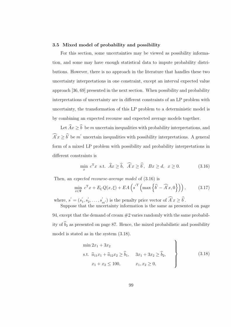
3.5 Mixed model of probability and possibility

For this section, some uncertainties may be viewed as possibility informa-

tion, and some may have enough statistical data to impute probability distri-

butions. However, there is no approach in the literature that handles these two

uncertainty interpretations in one constraint, except an interval expected value

approach [36, 69] presented in the next section. When possibility and probability

interpretations of uncertainty are in different constraints of an LP problem with

uncertainty, the transformation of this LP problem to a deterministic model is

by combining an expected recourse and expected average models together.

Let Ax ≥ b be m uncertain inequalities with probability interpretations, and

A′x ≥ b′ be m′uncertain inequalities with possibility interpretations. A general

form of a mixed LP problem with possibility and probability interpretations in

different constraints is

minx

cTx s.t. Ax ≥ b, A′x ≥ b′ , Bx ≥ d, x ≥ 0. (3.16)

Then, an expected recourse-average model of (3.16) is

minx∈Ψ

cTx + Eξ Q(x, ξ) + EA(s′T(max

b′ − A′x, 0

)), (3.17)

where, s′= (s

′

1, s′

2, . . . , s′

m′ ) is the penalty price vector of A′x ≥ b′ .

Suppose that the uncertainty information is the same as presented on page

94, except that the demand of cream #2 varies randomly with the same probabil-

ity of b2 as presented on page 87. Hence, the mixed probabilistic and possibility

model is stated as in the system (3.18).

min 2x1 + 3x2

s.t. a11x1 + a12x2 ≥ b1, 3x1 + 3x2 ≥ b2,

x1 + x2 ≤ 100, x1, x2 ≥ 0,

(3.18)

99

where

a11 =

1 with Pos (1) = 13,

2 with Pos (2) = 1,

3 with Pos (3) = 12,

and a12 =

5 with Pos (5) = 13,

6 with Pos (6) = 34,

7 with Pos (7) = 1.

b1 =

149 with Pos (149) = 12,

180 with Pos (180) = 1,

211 with Pos (211) = 23,

and b2 =

138 with Pr (138) = 14,

162 with Pr (162) = 12,

185 with Pr (185) = 14.

Problem (3.18) is not well-defined until we know a realization of the uncer-

tainties. It is also not the same as problem (3.14), since b2 now has probability

interpretation. Applying recourse variables to the probabilitistic constraints and

using the expected average for possibilistic constraints, the expected recourse-

average of (3.18) is

min 2x1 + 3x2 + Eb2

Q(x, b2) + EA(7 max

b1 − a11x1 − a12x2, 0

)

s.t. x1 + x2 ≤ 100,

x1, x2 ≥ 0,

(3.19)

where Q(x, b2) = max 12y s.t. 3x1 + 3x2 + y(bi2) ≥ bi

2, y ≥ 0, and b12 =

138, b22 = 162, and b3

2 = 185.

An optimal solution for (3.19) is (x∗1, x2∗) = (45.63, 16.04), and the optimal

objective value is $139.37. This result happens to be the same as one for (3.14).

However, the semantic of the objective value for (3.14), through the mathemat-

ical definitions of expected value and expected average, is different from the

semantic of the objective value for (3.19), as you may see. A similar question as

in the last section has raised here as well. Moreover, this approach (of treating a

100

probability as a recourse model and a possibility as a penalized expected average

model) is suitable only when each constraint has only one type of uncertainty,

(either probability or possibility).

3.6 Mixed uncertainties model

We can apply an expected recourse function to the objective function of an

LP problem with uncertainty when all uncertainties in a constraint have proba-

bility interpretations. Similarly, we use expected average when all uncertainties

in a constraint are possibilities. However, it might happen that there is more

than one interpretation of uncertainty in one constraint. In this case, an ex-

pected recourse-average approach is no longer suitable. Lodwick and Jamison

[36] introduced the concept of interval expected value to handle this type of

problem.

Let U = u1 < u2 < . . . < ul be the set of all realizations of an uncertainty

u, and i : P(U) → Int[0,1] be an IVPM generated from consistent necessity,

Nec, and possibility, Pos, measures (see Definition 2.28). Then, the inter-

val expected value of this IVPM is constructed from possibility and necessity

measures as the specific upper and lower cumulative probability distributions,

respectively. The upper cumulative probability distribution denoted by F is

defined as F (uk) = Pos (u1, u2, . . . , uk). The lower cumulative probability

distribution F is defined as F (uk) = Nec (u1, u2, . . . , uk). The interval ex-

pected value is defined in [36] as E(i) =

[l∑

k=1

ukf(uk),l∑

k=1

ukf(uk)

], where f

and f refer to the probability density mass functions associated with F and F ,

respectively. It turns out that these f and f are the same density functions from

101

the construction (2.42) and (2.43) on page 39, because

f(uk) = F (uk)− F (uk−1)

= Pos (u1, u2, . . . , uk)− Pos (u1, u2, . . . , uk−1)

= (1−Nec (uk+1, uk+2 . . . , un))− (1−Nec (uk, uk+1 . . . , un))

= Nec (uk, uk+1 . . . , un)−Nec (uk+1, uk+2 . . . , un) , and

f(uk) = F (uk)− F (uk−1)

= Nec (u1, u2 . . . , uk)−Nec (u1, u2 . . . , uk−1) .

Let E(A) be an interval expected value matrix generated by an uncertainty

matrix A, and E(b) be an interval expected value vector generated by an uncer-

tainty vector b. [36, 69] transform an LP with mixed possibility and probability

interpretations of uncertainty to an interval linear programming by changing all

uncertainties to their interval expected values, as shown in (3.20). We call this

transformed model as an interval expected value model.

min cTx

s.t. Ax ≥ b

Bx ≥ d

x ≥ 0

⇒

min cTx

s.t. E(A)x ≥ E(b)

Bx ≥ d

x ≥ 0.

(3.20)

Although the uncertainty interpretations presented in [36, 69] are only prob-

ability and possibility, the relationships among different uncertainty interpreta-

tions in Chapter 2 imply that an interval expected value approach is suitable

for other PC-BRIN uncertainty interpretations as well. However, for the same

reason why we are not using the expected values to represent an LP problem

with probability uncertainty, the interval expected value approach is a limited

102

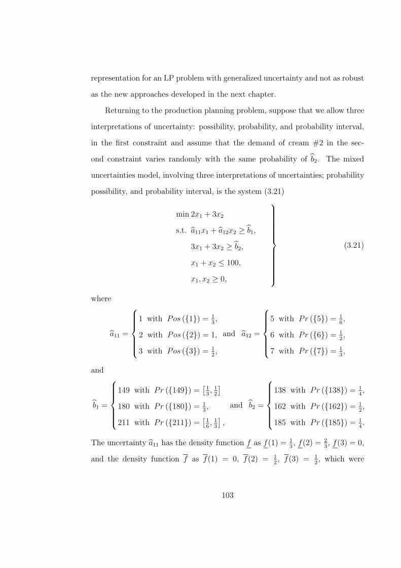
representation for an LP problem with generalized uncertainty and not as robust

as the new approaches developed in the next chapter.

Returning to the production planning problem, suppose that we allow three

interpretations of uncertainty: possibility, probability, and probability interval,

in the first constraint and assume that the demand of cream #2 in the sec-

ond constraint varies randomly with the same probability of b2. The mixed

uncertainties model, involving three interpretations of uncertainties; probability

possibility, and probability interval, is the system (3.21)

min 2x1 + 3x2

s.t. a11x1 + a12x2 ≥ b1,

3x1 + 3x2 ≥ b2,

x1 + x2 ≤ 100,

x1, x2 ≥ 0,

(3.21)

where

a11 =

1 with Pos (1) = 13,

2 with Pos (2) = 1,

3 with Pos (3) = 12,

and a12 =

5 with Pr (5) = 16,

6 with Pr (6) = 12,

7 with Pr (7) = 13,

and

b1 =

149 with Pr (149) =[

13, 1

2

]

180 with Pr (180) = 13,

211 with Pr (211) =[

16, 1

3

],

and b2 =

138 with Pr (138) = 14,

162 with Pr (162) = 12,

185 with Pr (185) = 14.

The uncertainty a11 has the density function f as f(1) = 13, f(2) = 2

3, f(3) = 0,

and the density function f as f(1) = 0, f(2) = 12, f(3) = 1

2, which were

103

obtained by applying the construction (2.42) and (2.43). Therefore, the interval

expected value of a11 is [1.6667, 2.5]. Similarly, we can get the interval expected

value of b1 as [169.6667, 180]. The LP problem with mixed uncertainty (3.21)

becomes an interval expected value model, which is the following interval linear

programming problem after applying the interval expected value for each of the

uncertainties.

min 2x1 + 3x2

s.t. [1.6667, 2.5] x1 + 6.1667x2 ≥ [169.6667, 180] ,

3x1 + 3x2 ≥ 161.75,

x1 + x2 ≤ 100,

x1, x2 ≥ 0.

(3.22)

The model (3.22) is also not well-defined. However, the bound on the objective

value is [$117.35, $127.87] with an optimal solution x1 ∈ [33.89, 44.41], and x2 ∈

[9.51, 20.03], which are obtained by solving four LP problems generated by the

endpoints of the first constraint of (3.22). We can see for example that ‘1’ and

‘3’ as the realizations of a11 are not in [1.6667, 2.5]. It is also clear that

a11 =

1 with Pr(1) = 14∈ [Nec(1), Pos(1)] =

[f(1), f(1)

]=[0, 1

3

],

2 with Pr(2) = 12∈ [Nec(2), Pos(2)] =

[f(2), f(2)

]=[

12, 2

3

],

3 with Pr(3) = 14∈ [Nec(3), Pos(3)] =

[f(3), f(3)

]=[0, 1

2

],

b1 =

149 with Pr(149) = 512∈[

13, 1

2

],

180 with Pr(180) = 13,

211 with Pr(211) = 14∈[

16, 1

3

],

but in the long run, an optimal solution based on this information (see Sub-

section 3.2.1), is x1 = 31.80 /∈ [33.89, 44.41], and x2 = 29.87 /∈ [9.51, 20.03].

104

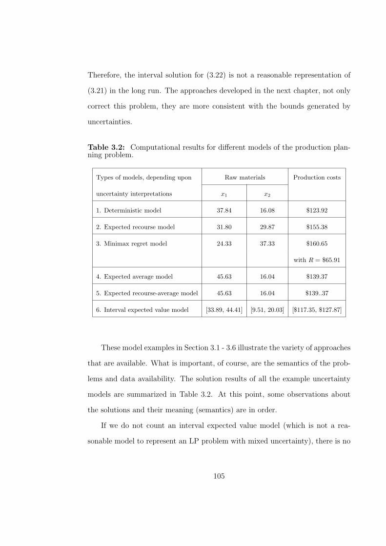
Therefore, the interval solution for (3.22) is not a reasonable representation of

(3.21) in the long run. The approaches developed in the next chapter, not only

correct this problem, they are more consistent with the bounds generated by

uncertainties.

Table 3.2: Computational results for different models of the production plan-ning problem.

Types of models, depending upon Raw materials Production costs

uncertainty interpretations x1 x2

1. Deterministic model 37.84 16.08 $123.92

2. Expected recourse model 31.80 29.87 $155.38

3. Minimax regret model 24.33 37.33 $160.65

with R = $65.91

4. Expected average model 45.63 16.04 $139.37

5. Expected recourse-average model 45.63 16.04 $139..37

6. Interval expected value model [33.89, 44.41] [9.51, 20.03] [$117.35, $127.87]

These model examples in Section 3.1 - 3.6 illustrate the variety of approaches

that are available. What is important, of course, are the semantics of the prob-

lems and data availability. The solution results of all the example uncertainty

models are summarized in Table 3.2. At this point, some observations about

the solutions and their meaning (semantics) are in order.

If we do not count an interval expected value model (which is not a rea-

sonable model to represent an LP problem with mixed uncertainty), there is no

105

research on an approach dealing with different types of uncertainty in one con-

straint. Furthermore, as the argument made at the end of Section 3.4, we do not

see that an expected average model and an expected recourse-average model are

reasonable representations for their associated uncertainty information. There-

fore, we introduce three expected recourse based models: (1) optimistic expected

recourse model, (2) pessimistic expected recourse model, and (3) minimax re-

gret problem of all expected recourse models, with the help of Theorems 2.17,

and 2.25. We develop the theories and illustrate some applications of linear

optimizations under generalized uncertainty in Chapters 4 and 5.

106

4. Linear optimization under uncertainty: pessimistic, optimistic,

and minimax regret approaches

Stochastic optimization is a well-known approach for mathematical pro-

grams with uncertainty. It is suitable when uncertainties are random parameters

with known probability distributions. The uncertainty with a known probabil-

ity distribution is called a probability interpretation of uncertainty. However, we

may not have complete information on these random parameters sufficient to

model them as probability distributions. This dissertation considers linear pro-

grams with PC-BRIN uncertainty interpretations. Consider a general form of a

linear problem with generalized uncertainty (1.2). Let us expand the uncertainty

constraints of (1.2) out term-by-term as follows:

minx

c1x1 + c2x2 + . . . + cnxn

s.t. a11x1 + a12x2 + . . . + a1nxn ≥ b1,

a21x1 + a22x2 + . . . + a2nxn ≥ b2,

...

am1x1 + am2x2 + . . . + amnxn ≥ bm,

Bx ≥ 0,

x ≥ 0,

(4.1)

where aij (and bi), i = 1, 2, . . . ,m and j = 1, 2, . . . , n, can be given as one of PC-

BRIN uncertainty interpretations. It could be that more than one interpretation

of uncertainty appears in one constraint. We introduce a new variable z when

there are uncertainties in an objective coefficient. Then, we add a constraint

107

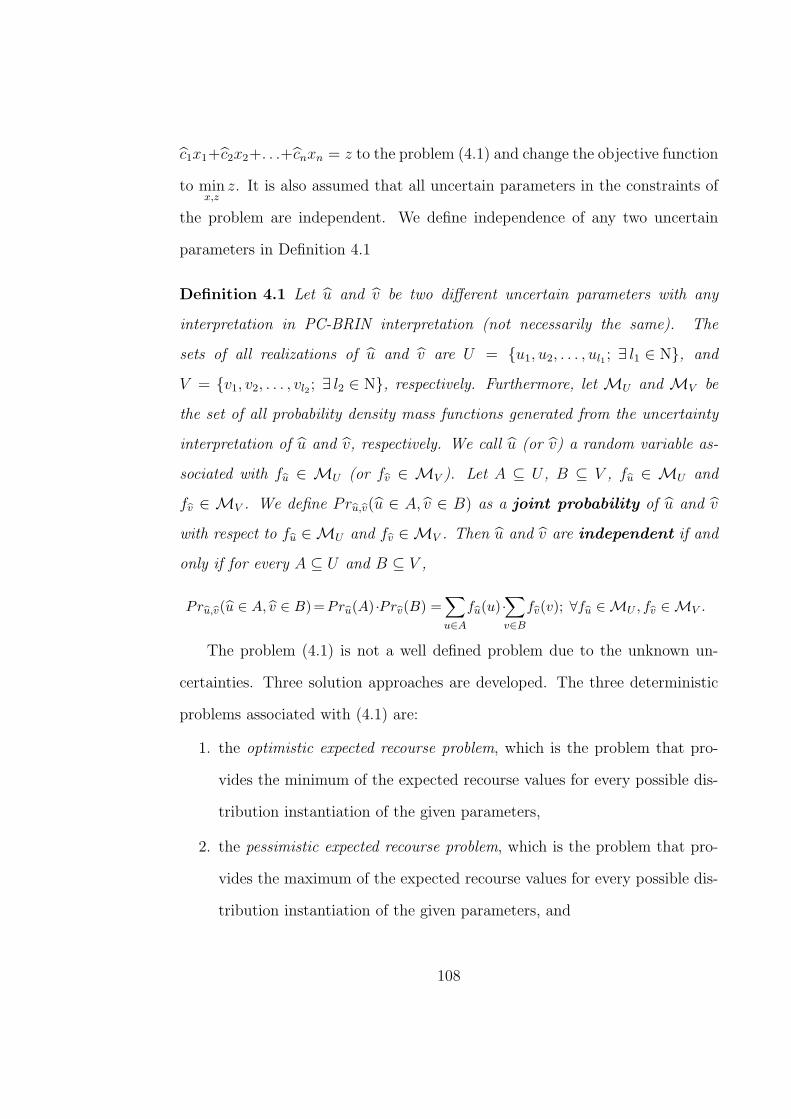
c1x1+c2x2+. . .+cnxn = z to the problem (4.1) and change the objective function

to minx,z

z. It is also assumed that all uncertain parameters in the constraints of

the problem are independent. We define independence of any two uncertain

parameters in Definition 4.1

Definition 4.1 Let u and v be two different uncertain parameters with any

interpretation in PC-BRIN interpretation (not necessarily the same). The

sets of all realizations of u and v are U = u1, u2, . . . , ul1 ; ∃ l1 ∈ N, and

V = v1, v2, . . . , vl2 ; ∃ l2 ∈ N, respectively. Furthermore, let MU and MV be

the set of all probability density mass functions generated from the uncertainty

interpretation of u and v, respectively. We call u (or v) a random variable as-

sociated with fu ∈ MU (or fv ∈ MV ). Let A ⊆ U , B ⊆ V , fu ∈ MU and

fv ∈ MV . We define Pru,v(u ∈ A, v ∈ B) as a joint probability of u and v

with respect to fu ∈MU and fv ∈MV . Then u and v are independent if and

only if for every A ⊆ U and B ⊆ V ,

Pru,v(u ∈ A, v ∈ B)=Pru(A) ·Prv(B) =∑

u∈A

fu(u) ·∑

v∈B

fv(v); ∀fu ∈MU , fv ∈MV .

The problem (4.1) is not a well defined problem due to the unknown un-

certainties. Three solution approaches are developed. The three deterministic

problems associated with (4.1) are:

1. the optimistic expected recourse problem, which is the problem that pro-

vides the minimum of the expected recourse values for every possible dis-

tribution instantiation of the given parameters,

2. the pessimistic expected recourse problem, which is the problem that pro-

vides the maximum of the expected recourse values for every possible dis-

tribution instantiation of the given parameters, and

108

3. the minimax regret problem of all expected recourse models, which is the

problem that provides the minimum of the maximum regret due to not

knowing the actual probability to establish an expected recourse model.

We discuss each of these problems in Sections 4.1 and 4.2.

4.1 Pessimistic and optimistic expected recourse problems

We explain the problem (4.1) as a refinery production plan problem that has

finite realizations of uncertainties. The first priority of the refinery is to satisfy

the demands of its clients while minimizing its productivity cost. So, the amount

of any shortage has to be bought from a market, incurring penalty (recourse)

costs to the refinery. We suppose that penalty costs are fixed throughout the

dissertation. We will not consider the storage cost or the selling cost of the

excess products at this moment.

We first assume that each of aij has αij realizations, a1ij, a

2ij, . . . , a

αij

ij , with

probability density mass values gij(a1ij), gij(a

2ij), . . . , gij(a

αij

ij ), and each of bi

has βi realizations, b1i , b

2i , . . . , b

βi

i , with probability density mass values hi(b1i ),

hi(b2i ), . . . , hi(b

βi

i ), where

αij∑

k=1

gij(akij) = 1, and

βi∑

k=1

hi(bki ) = 1. Instead of ran-

dom variables aij and bi, i = 1, 2, . . . m, j = 1, 2, . . . , n, we define the ran-

dom vector ξ =(a11, a12 . . . , amn, b1, b2 . . . , bm

). This random vector ξ cre-

atesn∏

j=1

m∏

i=1

αij · βi = N scenarios for constraints of (4.1). We introduce a

recourse variable yki = max

0, bi(ξ

k)− ai1(ξk)x1 − ai2(ξ

k)x2 − . . .− ain(ξk)xn

for each of the ith constraint in (4.1) and each kth scenario, i = 1, 2, . . . ,m, k =

1, 2, . . . , N . The recourse variable measures the corresponding shortage in pro-

duction if there is any. Assume further that the positive penalty price per unit

109

of shortages is the fixed value si for each ith constraint of (4.1), i.e., the penalty

price s1 corresponds with recourse variables y11, y

21, . . . , y

N1 , the penalty price

s2 corresponds with recourse variables y12, y

22, . . . , y

N2 , and so on. Hence, the

expected recourse problem of (4.1) when all uncertainties have finite discrete

probabilities is to minimize the sum of the production (first-stage) costs and the

expected recourse costs and can be formulated as the following problem where

(ξk, prk) (corresponding to yk) contains a realization of the kth scenario and its

joint probability density mass value prk such that∑N

k=1 prk = 1:

min c1x1 + c2x2 + . . . + cnxn +∑N

k=1 prk

[s1y

k1 + s2y

k2 + . . . + smyk

m

]

s.t. a11(ξk)x1 + a12(ξ

k)x2 + . . . + a1n(ξk)xn + yk1 ≥ b1(ξ

k), ∀k

a21(ξk)x1 + a22(ξ

k)x2 + . . . + a2n(ξk)xn + yk2 ≥ b2(ξ

k), ∀k

...

am1(ξk)x1 + am2(ξ

k)x2 + . . . + amn(ξk)xn + ykm ≥ bm(ξk), ∀k

Bx ≥ d, x, y ≥ 0.

(4.2)

We rewrite the problem (4.2) by keeping recourse variables on one side and

moving the rest to the other side of the inequalities, i.e.,

min c1x1 + c2x2 + . . . + cnxn +∑N

k=1 prk

[s1y

k1 + s2y

k2 + . . . + smyk

m

]

s.t. yk1 ≥ b1(ξ

k)− a11(ξk)x1 − a12(ξ

k)x2 − . . .− a1n(ξk)xn, ∀k

yk2 ≥ b2(ξ

k)− a21(ξk)x1 − a22(ξ

k)x2 − . . .− a2n(ξk)xn, ∀k

...

ykm ≥ bm(ξk)− am1(ξ

k)x1 − am2(ξk)x2 − . . .− amn(ξk)xn, ∀k

Bx ≥ d, x, y ≥ 0.

(4.3)

110

Define Ki =n∏

j=1

αij · βi to be the number of scenarios with respect to the ith

constraint of (4.1), for each i = 1, 2, . . . ,m. According to constraints in (4.3),

there are Mi =m∏

t=1,t 6=i

n∏

j=1

αtj · βt constraints from

yki ≥ bi(ξ

k)− ai1(ξk)x1 − ai2(ξ

k)x2 − . . .− ain(ξk)xn, k = 1, 2, . . . , N, (4.4)

that have the same scenario with respect to the ith constraint of (4.1). Thus there

are Ki groups of (4.4), each containing Mi constraints with the same scenario

of the ith constraint, i.e., KiMi = N , for each i = 1, 2, . . . ,m. More precisely,

suppose that yk1i , yk2

i , . . . , ykMi−1

i and ykMi

i have the same scenario with respect to

the ith constraint, when bli, a

l1i1, a

l2i2, . . . , a

lnin are realizations of bi, ai1, ai2, . . . , ain,

respectively. Therefore,

yk1i ≥ bl

i − al1i1x1 − al2

i2x2 − . . .− alninxn,

yk2i ≥ bl


i2x2 − . . .− alninxn,

...

ykMi

i ≥ bli − al1

i1x1 − al2i2x2 − . . .− aln

inxn.

However, since yki = max

0, bl


i2x2 − . . .− alninxn

for each k =

k1, k2, . . . , kMi, it turns out that yk1

i = yk2i = . . . = y

kMt

i . We define wLi = yk1

i ,

where L is the scenario (l, l1, l2, . . . , ln). The joint probability for wLi is fL

i , where

fLi = prk1 + prk2 + . . . + prkMi

= hi(bli)gi1(a

l1i1)gi2(a

l2i2) . . . gin(aln

in).

We provide a small numerical example here for a better understanding of this

paragraph.

111

Example 12.

min 2x1 + 3x2

s.t. a11x1 + 6x2 ≥ b1 (4.5)

3x1 + a22x2 ≥ b2 (4.6)

x ≥ 0,

where each of the uncertainties has 2 realizations together with their probability

density mass values. The details are

a11 =

1, P r(1) = 16

2, P r(2) = 56,

a22 =

2, P r(2) = 14

3, P r(3) = 34,

b1 =

170, P r(170) = 13

180, P r(180) = 23,

b2 =

160, P r(160) = 12

162, P r(162) = 12.

The expected recourse problem with penalty prices s1 = 5 and s2 = 7 is

min 2x1 + 3x2 +∑16

k=1 prk

[5yk

1 + 7yk2

]

s.t. y11 ≥ 170− 1x1 − 6x2, y1

2 ≥ 160− 3x1 − 2x2,

y21 ≥ 170− 1x1 − 6x2, y2

2 ≥ 162− 3x1 − 2x2,

y31 ≥ 170− 1x1 − 6x2, y3

2 ≥ 160− 3x1 − 3x2,

y41 ≥ 170− 1x1 − 6x2, y4

2 ≥ 162− 3x1 − 3x2,

...

y131 ≥ 180− 2x1 − 6x2, y13

2 ≥ 160− 3x1 − 2x2,

y141 ≥ 180− 2x1 − 6x2, y14

2 ≥ 162− 3x1 − 2x2,

y151 ≥ 180− 2x1 − 6x2, y15

2 ≥ 160− 3x1 − 3x2,

y161 ≥ 180− 2x1 − 6x2, y16

2 ≥ 162− 3x1 − 3x2,

x, y ≥ 0.

(4.7)

112

There are 4 scenarios with respect to constraint (4.5), i.e., (a11, b1) = (1, 170),

(2, 170), (1, 180) and (2, 180). We define w11 = y1

1 = y21 = y3

1 = y41, w2

1 = y51 =

y61 = y7

1 = y81, w3

1 = y91 = y10

1 = y111 = y12

1 , and w41 = y13

1 = y141 = y15

1 = y161 . The

joint probabilities of w11, w

21, w

31 and w4

1 are

f 11 =

(1

3

1

6

1

2

1

4

)+

(1

3

1

6

1

2

3

4

)+

(1

3

1

6

1

2

1

4

)+

(1

3

1

6

1

2

3

4

)=

1

3·1

6=

1

18,

f 21 =

(1

3

5

6

1

2

1

4

)+

(1

3

5

6

1

2

3

4

)+

(1

3

5

6

1

2

1

4

)+

(1

3

5

6

1

2

3

4

)=

1

3·5

6=

5

18,

f 31 =

(2

3

1

6

1

2

1

4

)+

(2

3

1

6

1

2

3

4

)+

(2

3

1

6

1

2

1

4

)+

(2

3

1

6

1

2

3

4

)=

2

3·1

6=

2

18,

f 41 =

(2

3

5

6

1

2

1

4

)+

(2

3

5

6

1

2

3

4

)+

(2

3

5

6

1

2

1

4

)+

(2

3

5

6

1

2

3

4

)=

2

3·5

6=

10

18.

Similarly, we define w12 = y1

2 = y52 = y9

2 = y132 , w2

2 = y22 = y6

2 = y102 = y14

2 , w32 =

y32 = y7

1 = y111 = y15

1 , and w42 = y4

1 = y81 = y12

1 = y161 . The joint probabilities

of w12, w

22, w

32, and w4

2 are f 12 = 1

2· 1

4= 1

8, f 2

2 = 12· 3

4= 3

8, f 3

2 = 12· 1

4= 1

8, and

f 42 = 1

2· 3

4= 3

8, respectively. We can transform the problem (4.7) to

min 2x1 + 3x2 + 5∑4

L=1 fL1 wL

1 + 7∑4

L=1 fL2 wL

2

s.t. w11 ≥ 170− 1x1 − 6x2, w1

2 ≥ 160− 3x1 − 2x2,

w21 ≥ 170− 2x1 − 6x2, w2

2 ≥ 160− 3x1 − 3x2,

w31 ≥ 180− 1x1 − 6x2, w3

2 ≥ 162− 3x1 − 2x2,

w41 ≥ 180− 2x1 − 6x2, w4

2 ≥ 162− 3x1 − 3x2, x, w ≥ 0. ♦

(4.8)

The transformation of (4.5) and (4.6) into (4.8) indicates how, in general,

the problem (4.3) can be remodeled. The reduced expected recourse model is:

113

minx∈Ψ

c1x1 + c2x2 + . . . + cnxn+

s1

∑K1

L=1 fL1 wL

1 + s2

∑K2

L=1 fL2 wL

2 + . . . + sm

∑Km

L=1 fLmwL

m

s.t. w11 ≥ b1

1 − a111x1 − a1

12x2 − . . .− a11nxn,

...

wK11 ≥ bβ1

1 − aα1111 x1 − aα12

12 x2 − . . .− aα1n

1n xn,

...

w1m ≥ b1

m − a1m1x1 − a1

m2x2 − . . .− a1mn,

...

wKmm ≥ bβm

m − aαm1m1 x1 − aαm2

m2 x2 − . . .− aαmnmn xn, w ≥ 0,

(4.9)

where

Ki∑

L=1

fLi = 1 for each i = 1, 2, . . . ,m. The original expected recourse model

(4.3) has n components of variable x and mN terms of the recourse variable

y. Thus, it has the total of mN + n unknown variables and mN constraints

(with respected to the uncertainties). On the other hand, the reduced expected

recourse model (4.9) has n +m∑

i=1

Ki unknown variables withm∑

i=1

Ki constraints

(with respected to the uncertainties). Since Mi ≥ 2, ∀ i = 1, 2, . . . ,m, mN =

K1M1 +K2M2 + . . .+KmMm ≥ 2∑m

i=1 Ki. Hence, (4.9) has at leastm∑

i=1

Ki less

variables and constraints than (4.3). The remodeled problem (4.9) reduces the

number of operations needed in each iteration of the simplex method compared

to the original expected recourse problem (4.3), in general, because the size of

the coefficient matrix of (4.9) is smaller than that of (4.3).

Uncertainties in the problem (4.1) also can have other interpretations in PC-

BRIN besides probability. Thus, instead of a single joint probability distribution

fLi , L = 1, 2, . . . , Ki, i = 1, 2, . . . ,m, as in the expected recourse problem (4.9),

114

we have a set of joint probabilities.

4.1.1 Pessimistic and optimistic expected recourse problems

generated by random sets with finite realizations

We consider any uncertain information in Figure 2.7 that can be interpreted

as a random set. Suppose that uncertainties aij and bi; ∀ i = 1, 2, . . . ,m, ∀ j =

1, 2, . . . , n, can be interpreted as random sets. Let Θaij=a1

ij, a2ij, . . . , a

αij

ij

be

the set of all realizations of aij, and Θbi=

b1i , b

2i , . . . , b

βi

i

be the set of all real-

izations of bi. Then, the sets of all probability density mass functions satisfying

the random set information of aij and bi areMaijandMbi

, respectively, where

Maij=

gij : Θaij→ [0, 1] |

∑

akij∈A

gij(akij) ∈ [Belij(A), P lij(A)] , ∀A ⊆ Θaij

,

Mbi=

hi : Θbi→ [0, 1] |

∑

bki ∈A

hi(bki ) ∈ [Beli(A), P li(A)] , ∀A ⊆ Θbi

.

Therefore, the term fi, ∀ i = 1, 2, . . . ,m, in the objective function of (4.9) is an

element of the setMi of all joint probabilities satisfying random set information

on the ith constraint of (4.1), where

Mi =

fi : Θbi

×n∏

j=1

Θaij→ [0, 1] |

Ki∑

L=1

fLi = 1, fL

i = hLi gL

i1gLi2 . . . gL

in

,

hi ∈ Mbi, gij ∈ Maij

, Ki = Πnj=1αijβi is the number of scenarios with respect

to the ith constraint of (4.1), hLi = hi(b

k1i ), ∃ bk1

i ∈ Θbi, and for each j, gL

ij =

gij(ak2ij ), ∃ ak2

ij ∈ Θaij.

Example 13 illustratesMaij,Mbi

, andMi using a small set of realizations.

115

Example 13. Suppose that uncertainties a11 and b1 in constraint (4.5)

of Example 12 do not have probability interpretations. Instead, two realiza-

tions, 1 and 2, of a11 and other two realizations, 170 and 180, of b1 have

random set information as follows: m (1) = 12,m (1, 2) = 1

2,m (170) =

13, and m (180) = 2

3. So,

Ma11 =

g11 | g11 (1) + g11 (2) = 1, g11 (1) ∈

[1

2, 1

], g11 (2) ∈

[0,

1

2

],

Mb1 =

h1 | h1 (170) + h1 (180) = 1, h1 (170) ∈

[1

3, 1

], h1 (180) ∈

[0,

2

3

].

There are K1 = 4 scenarios for constraint (4.5): 1) 1x1 + 6x2 ≥ 170, 2) 1x1 +

6x2 ≥ 180, 3) 2x1 +6x2 ≥ 170, and 4) 2x1 +6x2 ≥ 180. Thus, f1 in the objective

function of (4.8) is

M1 =

f1 |

4∑

L=1

fL1 = 1, fL

1 = hL1 gL

11, s.t. h1 ∈Mb1 , g11 ∈Ma11

.

• When L = 1, gL11 = g11(1), and hL

1 = h1(170).

• When L = 2, gL11 = g11(1), and hL

1 = h1(180).

• When L = 3, gL11 = g11(2), and hL

1 = h1(170).

• When L = 4, gL11 = g11(2), and hL

1 = h1(180).

Suppose g111 = g2

11 = 23, and h1

1 = h31 = 2

3, then g3

11 = g411 = 1

3, and h2

1 = h41 = 1

3.

Hence, f1 ∈M1, where f 11 = 4

9, f 2

1 = 29, f 3

1 = 29, and f 4

1 = 19. ♦

Random sets generate the set Mi of joint probabilities for each ith con-

straint of (4.1). The uncertainty interpretations that can be presented as

random sets are listed in Figure 2.7. Without any further information about

116

these uncertainties, we define Ξ as the feasible set of the constraints in (4.9),

andM := f = (f1, f2, . . . , fm) | fi ∈Mi, i = 1, 2, . . . ,m. Two important ap-

proaches are the pessimistic and optimistic ones for the expected recourse prob-

lems (4.9), ∀ f ∈M. The recourse problem for an optimistic solution is

minf∈M

min(x,w)∈Ξ

c1x1 + c2x2 + . . . + cnxn+

s1

∑K1

L=1 fL1 wL

1 + s2

∑K2

L=1 fL2 wL

2 + . . . + sm

∑Km

L=1 fLmwL

m

,(4.10)

and the recourse problem for a pessimistic solution is

maxf∈M

min(x,w)∈Ξ

c1x1 + c2x2 + . . . + cnxn+

s1

∑K1

L=1 fL1 wL

1 + s2

∑K2

L=1 fL2 wL

2 + . . . + sm

∑Km

L=1 fLmwL

m

.(4.11)

We refer to the problems (4.10) and (4.11) as the optimistic and pessimistic

expected recourse problems, respectively.

Theorem 4.2 Assume that all uncertainties are random sets. Let s = [s1, s2,

. . . , sm]T, f = (f1, f2, . . . , fm) ∈M, fi =[f 1

i , f 2i , . . . , fKi

i

]such that

∑Ki

L=1 fLi =

1, and wi =[w1

i , w2i , . . . , w

Ki

i

]T, i = 1, 2, . . . ,m. Suppose that

min(x,w)∈Ξ

c1x1 + c2x2 + . . . + cnxn+

s1

∑K1

L=1 fL1 wL

1 + s2

∑K2

L=1 fL2 wL

2 + . . . + sm

∑Km

L=1 fLmwL

m

(4.12)

is bounded for each f ∈ M. Then, there exist f and f ∈ M, which can be

constructed, such that

minf∈M

min(x,w)∈Ξ

cTx + sT

f1w1

...

fmwm

= min(x,w)∈Ξ

cTx + sT

f1w1

...

fm

wm

, (4.13)

and

117

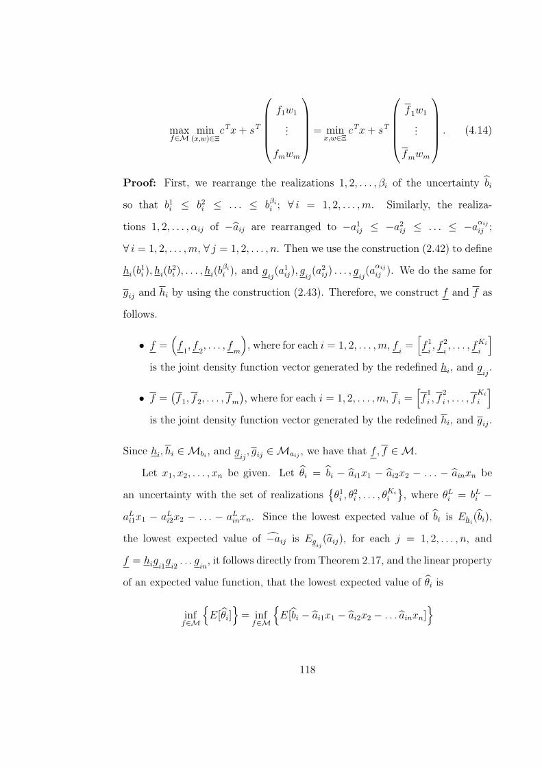
maxf∈M

min(x,w)∈Ξ

cTx + sT

f1w1

...

fmwm

= minx,w∈Ξ

cTx + sT

f 1w1

...

fmwm

. (4.14)

Proof: First, we rearrange the realizations 1, 2, . . . , βi of the uncertainty bi

so that b1i ≤ b2

i ≤ . . . ≤ bβi

i ; ∀ i = 1, 2, . . . ,m. Similarly, the realiza-

tions 1, 2, . . . , αij of −aij are rearranged to −a1ij ≤ −a2

ij ≤ . . . ≤ −aαij

ij ;

∀ i = 1, 2, . . . ,m, ∀ j = 1, 2, . . . , n. Then we use the construction (2.42) to define

hi(b1i ), hi(b

2i ), . . . , hi(b

βi

i ), and gij(a1

ij), gij(a2

ij) . . . , gij(a

αij

ij ). We do the same for

gij and hi by using the construction (2.43). Therefore, we construct f and f as

follows.

• f =(f

1, f

2, . . . , f

m

), where for each i = 1, 2, . . . ,m, f

i=[f 1

i, f 2

i, . . . , fKi

i

]

is the joint density function vector generated by the redefined hi, and gij.

• f =(f 1, f 2, . . . , fm

), where for each i = 1, 2, . . . ,m, f i =

[f

1

i , f2

i , . . . , fKi

i

]

is the joint density function vector generated by the redefined hi, and gij.

Since hi, hi ∈Mbi, and g

ij, gij ∈Maij

, we have that f, f ∈M.

Let x1, x2, . . . , xn be given. Let θi = bi − ai1x1 − ai2x2 − . . . − ainxn be

an uncertainty with the set of realizationsθ1

i , θ2i , . . . , θ

Ki

i

, where θL

i = bLi −

aLi1x1 − aL

i2x2 − . . . − aLinxn. Since the lowest expected value of bi is Ehi

(bi),

the lowest expected value of −aij is Egij(aij), for each j = 1, 2, . . . , n, and

f = higi1g

i2. . . g

in, it follows directly from Theorem 2.17, and the linear property

of an expected value function, that the lowest expected value of θi is

inff∈M

E[θi]

= inf

f∈M

E [bi − ai1x1 − ai2x2 − . . . ainxn]

118

inff∈M

E[θi]

= inf

f∈M

Ehi

[bi] + Egi1[−ai1]x1 + Egi2

[−ai2]x2 + . . . + Egin[−ain]xn

where hi ∈Mbiand gij ∈Maij

, j = 1, 2, . . . , n

= Ehi[bi] + Eg

i1[−ai1]x1 + Eg

i2[−ai2]x2 + . . . + Eg

in[−ain]xn

= Ef [θi]

=

Ki∑

L=1

fL

iθL

i .

The largest expected value of θi can be obtained in similar pattern. There-

fore, the expected value of θi with respect to any density function vector

fi =[f 1

i , f 2i , . . . , fKi

i

]∈Mi is

Ki∑

L=1

fL

iθL

i ≤Ki∑

L=1

fLi θL

i ≤Ki∑

L=1

fL

i θLi . (4.15)

We can also see that by using joint density function, we can rewrite this

lowest expected value as

E(θi) =

αij∑

kj=1

∀ j=1,2,...,n

(Πn

j=1gkj

ij

)h1

i

θ1,k1,k2,...,kni︷︸︸︷

(b1i − ak1

i1 x1 − ak2i2 x2 − . . .− akn

in xn)

+ . . . + hβi

i

θβi,k1,k2,...,kni︷︸︸︷

(bβi

i − ak1i1 x1 − ak2

i2 x2 − . . .− akn

in xn)

, (4.16)

which means that the term h1i θ

1,k1,k2,...,kn

i +. . .+hβi

i θβi,k1,k2,...,kn

i is the smallest, for

each kj = 1, . . . , αij. Hence, the statement (4.15) also holds if we change θLi to 0

whenever θLi < 0. Here is the reason. For the fixed scenario indexes k1, k2, . . . , kn

of uncertainties ai1, ai2, . . . , ain, suppose that bki −ak1

i1 x1−ak2i2 x2− . . .−akn

in xn < 0,

for some k = 1, 2, . . . , βi. Then, it means bji −ak1

i1 x1−ak2i2 x2− . . .−akn

in xn < 0, for

119

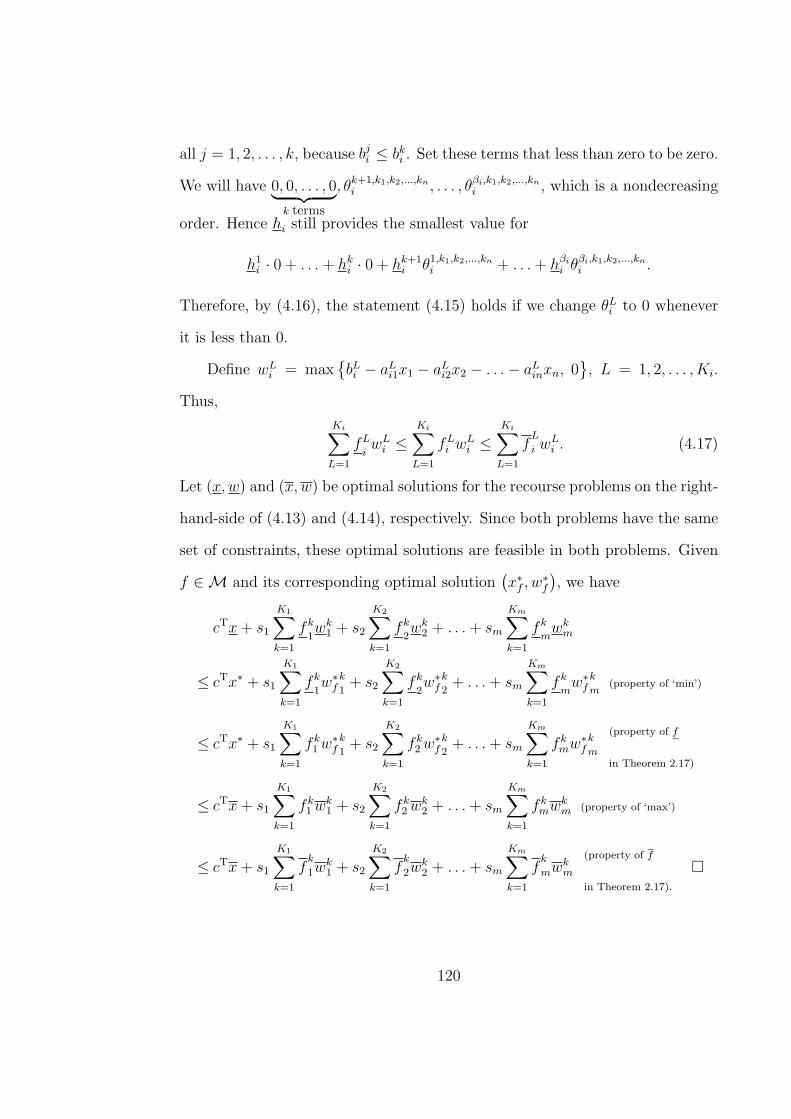
all j = 1, 2, . . . , k, because bji ≤ bk

i . Set these terms that less than zero to be zero.

We will have 0, 0, . . . , 0︸︷︷︸k terms

, θk+1,k1,k2,...,kn

i , . . . , θβi,k1,k2,...,kn

i , which is a nondecreasing

order. Hence hi still provides the smallest value for

h1i · 0 + . . . + hk

i · 0 + hk+1i θ1,k1,k2,...,kn

i + . . . + hβi

i θβi,k1,k2,...,kn

i .

Therefore, by (4.16), the statement (4.15) holds if we change θLi to 0 whenever

it is less than 0.

Define wLi = max

bLi − aL

i1x1 − aLi2x2 − . . .− aL

inxn, 0, L = 1, 2, . . . , Ki.

Thus,

Ki∑

L=1

fL

iwL

i ≤Ki∑

L=1

fLi wL

i ≤Ki∑

L=1

fL

i wLi . (4.17)

Let (x,w) and (x, w) be optimal solutions for the recourse problems on the right-

hand-side of (4.13) and (4.14), respectively. Since both problems have the same

set of constraints, these optimal solutions are feasible in both problems. Given

f ∈M and its corresponding optimal solution(x∗

f , w∗f

), we have

cTx + s1

K1∑

k=1

fk

1wk

1 + s2

K2∑

k=1

fk

2wk

2 + . . . + sm

Km∑

k=1

fk

mwk

m

≤ cTx∗ + s1

K1∑

k=1

fk

1w∗

fk

1+ s2

K2∑

k=1

fk

2w∗

fk

2+ . . . + sm

Km∑

k=1

fk

mw∗

fk

m(property of ‘min’)

≤ cTx∗ + s1

K1∑

k=1

fk1 w∗

fk

1+ s2

K2∑

k=1

fk2 w∗

fk

2+ . . . + sm

Km∑

k=1

fkmw∗

fk

m

(property of f

in Theorem 2.17)

≤ cTx + s1

K1∑

k=1

fk1 wk

1 + s2

K2∑

k=1

fk2 wk

2 + . . . + sm

Km∑

k=1

fkmwk

m (property of ‘max’)

≤ cTx + s1

K1∑

k=1

fk

1wk1 + s2

K2∑

k=1

fk

2wk2 + . . . + sm

Km∑

k=1

fk

mwkm

(property of f

in Theorem 2.17).

120

4.1.2 Pessimistic and optimistic expected recourse problems

generated by IVPMs with finite realizations

Suppose now that uncertainties aij and bi; ∀ i = 1, 2, . . . ,m, and ∀ j =

1, 2, . . . , n, can be interpreted as IVPMs. We use the same notation Maijand

Mbifor the sets of all probability measures satisfying the IVPM information of

aij and bi, respectively, where

Maij=

gij : Θaij→ [0, 1] |

∑

akij∈A

gij(akij) ∈ [Lij(A), Uij(A)] , ∀A ⊆ Θaij

,

and

Mbi=

hi : Θbi→ [0, 1] |

∑

bki ∈A

hi(bki ) = 1 ∈ [Li(A), Ui(A)] , ∀A ⊆ Θbi

.

Lij(A) and Uij(A) are the lower and upper bounds on probability gij of an event

A ⊆ Θaij. 0 ≤ Lij(A) ≤ Uij(A) ≤ 1. Similarly, Li(A) and Ui(A) are the

lower and upper bounds on probability hi of an event A ⊆ Θbi. 0 ≤ Li(A) ≤

Ui(A) ≤ 1. Then, using the same notationMi for the set of all joint probabilities

satisfying IVPM information on the ith constraint of (4.1), we also have

Mi =

fi : Θbi

×n∏

j=1

Θaij→ [0, 1] |

Ki∑

L=1

fLi = 1, fL

i = hLi gL

i1gLi2 . . . gL

in

,

DefineM := f = (f1, f2, . . . , fm) | fi ∈Mi, i = 1, 2, . . . ,m as in the last sub-

section, but keep in mind that information in this subsection is IVPM. We state

a similar theorem to Theorem 4.2 as follows.

Theorem 4.3 Assume that all uncertainties are IVPMs. Let s = [s1, s2,

. . . , sm]T, f = (f1, f2, . . . , fm) ∈M, fi =[f 1

i , f 2i , . . . , fKi

i

]such that

∑Ki

L=1 fLi =

1, and wi =[w1

i , w2i , . . . , w

Ki

i

]T, i = 1, 2, . . . ,m. Suppose that

121

min(x,w)∈Ξ

c1x1 + c2x2 + . . . + cnxn+

s1

∑K1

L=1 fL1 wL

1 + s2

∑K2

L=1 fL2 wL

2 + . . . + sm

∑Km

L=1 fLmwL

m



minf∈M

min(x,w)∈Ξ

cTx + sT

f1w1

...

fmwm

= min(x,w)∈Ξ

cTx + sT

f1w1

...

fm

wm

,

and

maxf∈M

min(x,w)∈Ξ

cTx + sT

f1w1

...

fmwm

= minx,w∈Ξ

cTx + sT

f 1w1

...

fmwm

.

Proof: Similar to the proof of Theorem 4.2, but use Theorem 2.25 instead of

Theorem 2.17 inside the proof.

Therefore, we can combine both Theorems 4.2 and 4.3 as Theorem 4.4, so

that the new theorem is applicable for any uncertainty interpretation in Figure

2.7. Use the same notationM to define the set of all joint probabilities. Hence,

M := f = (f1, f2, . . . , fm) | fi ∈Mi, i = 1, 2, . . . ,m, whereMi in this setM

is Mi =

fi |∑Ki

L=1 fLi = 1, fL

i = hLi gL

i1gLi2 . . . gL

in, s.t. hi ∈Mbi, gij ∈Maij

such that Mbiand Maij

are generated by either random set or IVPM infor-

mation. The proof of Theorem 4.4 is the combination of the proofs of Theorems

4.2 and 4.3.

Theorem 4.4 Assume that aij and bi can have PC-BRIN interpretation. Let

s = [s1, s2, . . . , sm]T, f = (f1, f2, . . . , fm) ∈M, fi =[f 1

i , f 2i , . . . , fKi

i

]such that

∑Ki

L=1 fLi = 1, and wi =

[w1

i , w2i , . . . , w

Ki

i

]T, i = 1, 2, . . . ,m. Suppose that

122

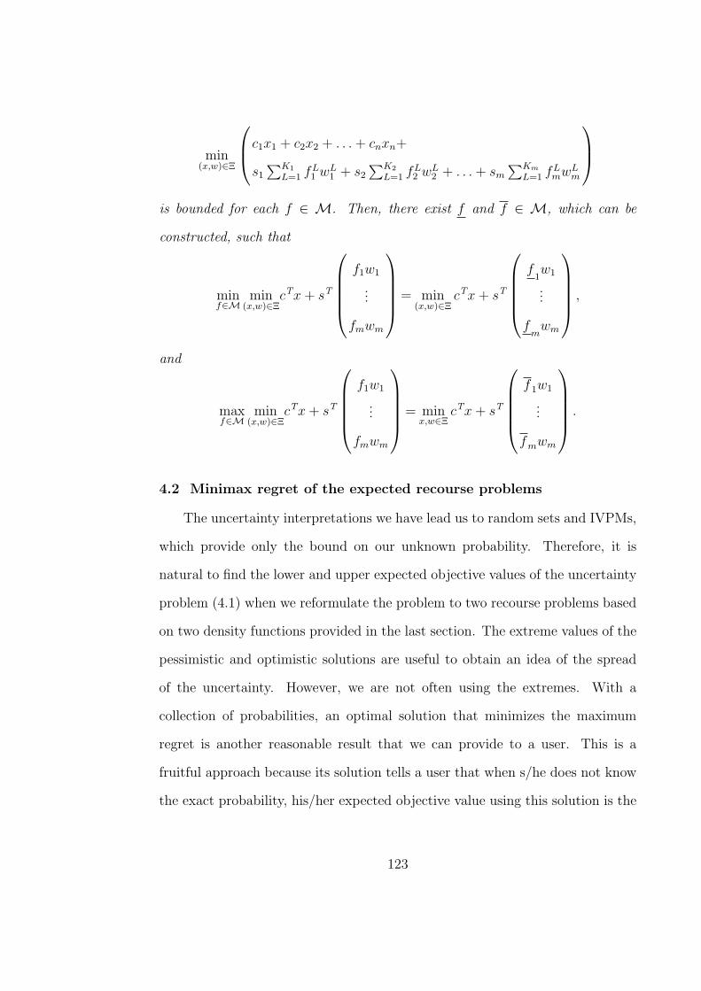
min(x,w)∈Ξ

c1x1 + c2x2 + . . . + cnxn+

s1

∑K1

L=1 fL1 wL

1 + s2

∑K2

L=1 fL2 wL

2 + . . . + sm

∑Km

L=1 fLmwL

m



minf∈M

min(x,w)∈Ξ

cTx + sT

f1w1

...

fmwm

= min(x,w)∈Ξ

cTx + sT

f1w1

...

fm

wm

,

and

maxf∈M

min(x,w)∈Ξ

cTx + sT

f1w1

...

fmwm

= minx,w∈Ξ

cTx + sT

f 1w1

...

fmwm

.

4.2 Minimax regret of the expected recourse problems

The uncertainty interpretations we have lead us to random sets and IVPMs,

which provide only the bound on our unknown probability. Therefore, it is

natural to find the lower and upper expected objective values of the uncertainty

problem (4.1) when we reformulate the problem to two recourse problems based

on two density functions provided in the last section. The extreme values of the

pessimistic and optimistic solutions are useful to obtain an idea of the spread

of the uncertainty. However, we are not often using the extremes. With a

collection of probabilities, an optimal solution that minimizes the maximum

regret is another reasonable result that we can provide to a user. This is a

fruitful approach because its solution tells a user that when s/he does not know

the exact probability, his/her expected objective value using this solution is the

123

best of the worst regret. We have the aim to solve the minimum of the maximum

regret (the minimax regret, for short) of the expected recourse problems (4.9),

with unknown probabilities of each uncertainty aij and bi in the set Maijand

Mbi. The uncertainty interpretations of aij and bi can be a random set or an

IVPM information.

Define the objective function of (4.9) as

z (f, x, w) := cTx + s1

K1∑

k=1

fk1 wk

1 + s2

K2∑

k=1

fk2 wk

2 + . . . + sm

Km∑

k=1

fkmwk

m.

We now consider the problem

min(x,w)∈Ξ

z (f, x, w) , (4.18)

which has uncertain probability f ∈ M. The regret with respect to a known

probability f , which shows the amount that a candidate solution (x,w) deviates

from the true objective value, can be expressed by

r(f, x, w) :=

(z (f, x, w)− min

(χ,ω)∈Ξz (f, χ, ω)

), (4.19)

where, min(χ,ω)∈Ξ

z (f, χ, ω) is the true solution with this known probability f .

When the true probability f is unknown, the worst (maximum) regret of a

candidate solution (x,w) is

R(x,w) := maxf∈M

r(f, x, w). (4.20)

The best of the worst regret over all candidate solutions is

min(x,w)∈Ξ

R(x,w). (4.21)

124

We rewrite the problem (4.21) as

min(x,w)∈Ξ

maxf∈M

(z (f, x, w)− min

(χ,ω)∈Ξz (f, χ, ω)

). (4.22)

Since − min(χ,ω)∈Ξ

z (f, χ, ω) = max(χ,ω)∈Ξ

(−z (f, χ, ω)), the problem (4.22) becomes

min(x,w)∈Ξ

maxf∈M

(z (f, x, w)− min

(χ,ω)∈Ξz (f, χ, ω)

)

= min(x,w)∈Ξ

maxf∈M

(z (f, x, w) + max

(χ,ω)∈Ξ(−z (f, χ, ω))

)

= min(x,w)∈Ξ

maxf∈M

(max

(χ,ω)∈Ξ(−z (f, χ, ω)) + z (f, x, w)

)

= min(x,w)∈Ξ

maxf∈M

(max

(χ,ω)∈Ξ(−z (f, χ, ω) + z (f, x, w))

)

= min(x,w)∈Ξ

maxf∈M

(max

(χ,ω)∈Ξ(z (f, x, w)− z (f, χ, ω))

)

= min(x,w)∈Ξ

maxf∈M

max(χ,ω)∈Ξ

(z (f, x, w)− z (f, χ, ω))

= min(x,w)∈Ξ

maxf∈M

(χ,ω)∈Ξ

(z (f, x, w)− z (f, χ, ω)) . (4.23)

4.2.1 A relaxation procedure for minimax regret of the expected

recourse problems

Literature on finding a minimax regret solution to a linear programming

problem, whose objective coefficients are not certain in a closed convex set, ap-

pears when the linear program has interval objective coefficients. The paper [1]

in 2009 surveys the recent work on this problem, and the latest found are in

[21, 22, 45, 46], and [62] which are based on a relaxation procedure to solve a

minimax problem of an LP with interval objective coefficients. The relaxation

procedure is effective for a class of problems with a very large number of con-

straints. We can transform the minimax regret problem (4.23) into the following

125

optimization problem with an infinite number of constraints:

minR, (x,w)

R

s.t. R ≥ (z (f, x, w)− z (f, χ, ω)) , ∀f ∈M and (χ, ω) ∈ Ξ

(x,w) ∈ Ξ

R ≥ 0.

(4.24)

Instead of solving this problem (4.24), we solve a series of the following relaxed

versions of the problem:

minR, (x,w)

R

s.t. (x,w) ∈ Ξ

R ≥ 0

R ≥(z(f (i), x, w

)− z

(f (i), χ(i), ω(i)

)); f (i) ∈M and (χ(i), ω(i)) ∈ Ξ,

i = 1, 2, . . . , k.

(4.25)

Let (x(k), w(k), R(k)) be optimal for the relaxed problem (4.25). If (x(k), w(k), R(k))

is feasible for the problem (4.24), then it must be optimal for the prob-

lem (4.24). Hence, (x(k), w(k)) is a minimax regret solution to the prob-

lem (4.23). On the other hand, if there exists at least one constraint from

R ≥ (z (f, x, w)− z (f, χ, ω)) , ∀f ∈M and (χ, ω) ∈ Ξ violates (x(k), w(k), R(k)),

then the most violated constraint will be added to the constraints of the relaxed

problem. Next, solve the updated problem setting k := k + 1 and repeating the

process. We can check which constraint is the most violated one by

1. if maxf∈M

(χ,ω)∈Ξ

(z(f, x(k), w(k)

)− z (f, χ, ω)

)≤ R(k), then obviously

(z(f, x(k), w(k)

)− z (f, χ, ω)

)≤ R(k), for all f ∈M and (χ, ω) ∈ Ξ,

126

2. if maxf∈M

(χ,ω)∈Ξ

(z(f, x(k), w(k)

)− z (f, χ, ω)

)> R(k),

then the most violated constraint to (x(k), w(k), R(k)) is(z(f (k+1), x(k), w(k)

)− z

(f (k+1), χ(k+1), ω(k+1)

))> R(k), where

(f (k+1), χ(k+1), ω(k+1)) is a solution to maxf∈M

(χ,ω)∈Ξ

(z(f, x(k), w(k)

)− z (f, χ, ω)

).

We conclude the relaxation procedure for minimax regret of expected recourse

problem in the following steps:

Algorithm 4.5 Relaxation procedure.

step 1: Initialization. Choose f (1) = f , and (χ(1), ω(1)) is an optimal solution

to the problem min(χ,ω)∈Ξ

z(f, χ, ω

). Set k = 1.

step 2: Solve the current relaxed problem

minR, (x,w)

R

s.t. (x,w) ∈ Ξ

R ≥ 0

R ≥(z(f (i), x, w

)− z

(f (i), χ(i), ω(i)

)), i = 1, 2, . . . , k,

and obtain an optimal solution (x(k), w(k), R(k)) for the relaxed problem.

step 3: Solve Z(k) = maxf∈M

(χ,ω)∈Ξ

(z(f, x(k), w(k)

)− z (f, χ, ω)

)

= maxf∈M

(z(f, x(k), w(k)

)− min

(χ,ω)∈Ξz (f, χ, ω)

),

and obtain an optimal solution (f (k+1), χ(k+1), ω(k+1)) and its optimal ob-

jective value Z(k).

step 4: If Z(k) ≤ R(k), terminate. A minimax regret optimal solution is

(x(k), w(k)). If Z(k) > R(k), set k = k + 1 and go back to step 2. ♦

127

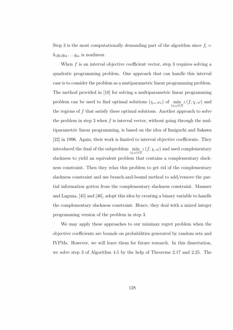
Step 3 is the most computationally demanding part of the algorithm since fi =

higi1gi2 . . . gin is nonlinear.

When f is an interval objective coefficient vector, step 3 requires solving a

quadratic programming problem. One approach that can handle this interval

case is to consider the problem as a mutiparametric linear programming problem.

The method provided in [18] for solving a multiparametric linear programming

problem can be used to find optimal solutions (χ∗, ω∗) of min(χ,ω)∈Ξ

z (f, χ, ω) and

the regions of f that satisfy these optimal solutions. Another approach to solve

the problem in step 3 when f is interval vector, without going through the mul-

tiparametric linear programming, is based on the idea of Inuiguchi and Sakawa

[22] in 1996. Again, their work is limited to interval objective coefficients. They

introduced the dual of the subproblem min(χ,ω)∈Ξ

z (f, χ, ω) and used complementary

slackness to yield an equivalent problem that contains a complementary slack-

ness constraint. Then they relax this problem to get rid of the complementary

slackness constraint and use branch-and-bound method to add/remove the par-

tial information gotten from the complementary slackness constraint. Mausser

and Laguna, [45] and [46], adopt this idea by creating a binary variable to handle

the complementary slackness constraint. Hence, they deal with a mixed integer

programming version of the problem in step 3.

We may apply these approaches to our minimax regret problem when the

objective coefficients are bounds on probabilities generated by random sets and

IVPMs. However, we will leave them for future research. In this dissertation,

we solve step 3 of Algorithm 4.5 by the help of Theorems 2.17 and 2.25. The

128

details follow. Consider

Z(k) = maxf∈M

(χ,ω)∈Ξ

(z(f, x(k), w(k)

)− z (f, χ, ω)

)

= maxf∈M

(χ,ω)∈Ξ

(cT(x(k) − χ) + s1

∑K1

j=1 fk1 (w

(k)j

1 − ωj1) + s2

∑K2

j=1 fk2 (w

(k)j

2 − ωj2)

+ . . . + sm

∑Km

j=1 fkm(w

(k)j

m − ωjm)).

We do not know the order of the components in the vector (w(k)i − ωi), for each

i. Therefore, we can not apply Theorem 4.4 directly to obtain Z(k). However,

fi is a joint density of aij, ∀ j = 1, 2, . . . , n and bi. Suppose an uncertainty

v has the set of all realizations V =v1, v2, . . . , vαij

, but we do not know the

ordering of these realizations. Suppose further that v has the same random set

or IVPM information as aij (or bi, when V = v1, v2, . . . , vβi). That is,Mv has

the same restrictions as Maij, where Mv is the set of all probability densities

satisfying the random set or IVPM information of v. Hence, vk is equivalent

to akij, ∀ k = 1, 2, . . . , αij, and Av = vk1 , vk2 , . . . , vkt

⊆ V is equivalent to

A =ak1

ij , ak2ij , . . . , akt

ij

⊆ Θaij

. For

Maij=

gij : Θaij→ [0, 1] |

∑

akij∈A

gij(akij) ∈ [Lij(A), Uij(A)] , ∀A ⊆ Θaij

,

we can writeMv as

Mv =

g : V → [0, 1] |∑

vk∈Av

g(vk) ∈ [L(Av), U(Av)] , ∀Av ⊆ V

,

such that g(vk) = gij(akij), ∀ k = 1, 2, . . . , αij, L(Av) = Lij(A), and U(Av) =

Uij(A). Using Theorems 2.17 or 2.25 (depending upon the interpretation of

uncertainty v) to solve the problems ming∈Mv

gTv, with all αij! orderings of v, we

129

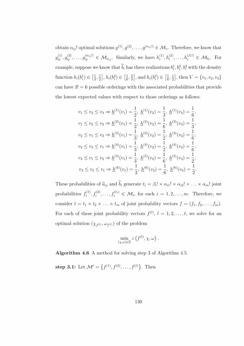
obtain αij! optimal solutions g(1), g(2), . . . , g(αij !) ∈Mv. Therefore, we know that

g(1)ij , g

(2)ij , . . . , g

(αij !)ij ∈ Maij

. Similarly, we have h(1)i , h

(2)i , . . . , h

(βi!)i ∈ Mbi

. For

example, suppose we know that bi has three realizations b1i , b

2i , b

3i with the density

function hi(b1i ) ∈

[13, 1

2

], hi(b

2i ) ∈

[16, 2

3

], and hi(b

3i ) ∈

[16, 1

2

], then V = v1, v2, v3

can have 3! = 6 possible orderings with the associated probabilities that provide

the lowest expected values with respect to those orderings as follows:

v1 ≤ v2 ≤ v3 ⇒ h(1)(v1) =1

2, h(1)(v2) =

1

3, h(1)(v3) =

1

6,

v1 ≤ v3 ≤ v2 ⇒ h(2)(v1) =1

2, h(2)(v2) =

1

6, h(2)(v3) =

1

3,

v2 ≤ v1 ≤ v3 ⇒ h(3)(v1) =1

3, h(3)(v2) =

1

2, h(3)(v3) =

1

6,

v2 ≤ v3 ≤ v1 ⇒ h(4)(v1) =1

3, h(4)(v2) =

1

2, h(4)(v3) =

1

6,

v3 ≤ v1 ≤ v2 ⇒ h(5)(v1) =1

3, h(5)(v2) =

1

6, h(5)(v3) =

1

2,

v3 ≤ v2 ≤ v1 ⇒ h(6)(v1) =1

3, h(6)(v2) =

1

6, h(6)(v3) =

1

2.

These probabilities of aij and bi generate ti = βi!× αi1!× αi2!× . . .× αin! joint

probabilities f(1)i , f

(2)i , . . . , f

(ti)i ∈ Mi, for each i = 1, 2, . . . ,m. Therefore, we

consider t = t1 × t2 × . . . × tm of joint probability vectors f = (f1, f2, . . . , fm).

For each of these joint probability vectors f (l), l = 1, 2, . . . , t, we solve for an

optimal solution (χf (l) , ωf (l)) of the problem

min(χ,ω)∈Ξ

z(f (l), χ, ω

).

Algorithm 4.6 A method for solving step 3 of Algorithm 4.5.

step 3.1: LetMt =f (1), f (2), . . . , f (t)

. Then

130

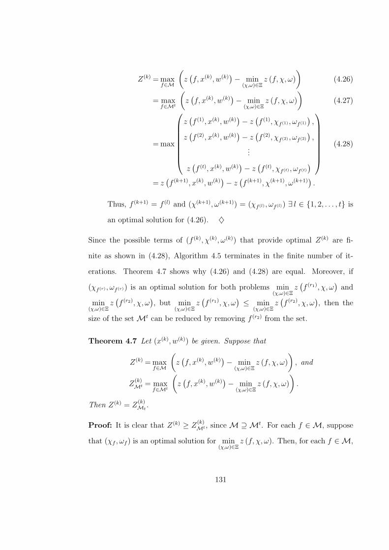
Z(k) = maxf∈M

(z(f, x(k), w(k)

)− min

(χ,ω)∈Ξz (f, χ, ω)

)(4.26)

= maxf∈Mt

(z(f, x(k), w(k)

)− min

(χ,ω)∈Ξz (f, χ, ω)

)(4.27)

= max

z(f (1), x(k), w(k)

)− z

(f (1), χf (1) , ωf (1)

),

z(f (2), x(k), w(k)

)− z

(f (2), χf (2) , ωf (2)

),

...

z(f (t), x(k), w(k)

)− z

(f (t), χf (t) , ωf (t)

)

(4.28)

= z(f (k+1), x(k), w(k)

)− z

(f (k+1), χ(k+1), ω(k+1)

).

Thus, f (k+1) = f (l) and (χ(k+1), ω(k+1)) = (χf (l) , ωf (l)) ∃ l ∈ 1, 2, . . . , t is

an optimal solution for (4.26). ♦

Since the possible terms of (f (k), χ(k), ω(k)) that provide optimal Z(k) are fi-

nite as shown in (4.28), Algorithm 4.5 terminates in the finite number of it-

erations. Theorem 4.7 shows why (4.26) and (4.28) are equal. Moreover, if

(χf (r) , ωf (r)) is an optimal solution for both problems min(χ,ω)∈Ξ

z(f (r1), χ, ω

)and

min(χ,ω)∈Ξ

z(f (r2), χ, ω

), but min

(χ,ω)∈Ξz(f (r1), χ, ω

)≤ min

(χ,ω)∈Ξz(f (r2), χ, ω

), then the

size of the setMt can be reduced by removing f (r2) from the set.

Theorem 4.7 Let (x(k), w(k)) be given. Suppose that

Z(k) = maxf∈M

(z(f, x(k), w(k)

)− min

(χ,ω)∈Ξz (f, χ, ω)

), and

Z(k)Mt = max

f∈Mt

(z(f, x(k), w(k)

)− min

(χ,ω)∈Ξz (f, χ, ω)

).

Then Z(k) = Z(k)Mt

.

Proof: It is clear that Z(k) ≥ Z(k)Mt , since M ⊇Mt. For each f ∈ M, suppose

that (χf , ωf ) is an optimal solution for min(χ,ω)∈Ξ

z (f, χ, ω). Then, for each f ∈M,

131

Z(k)f =

(z(f, x(k), w(k)

)− min

(χ,ω)∈Ξz (f, χ, ω)

)

=(z(f, x(k), w(k)

)− z (f, χf , ωf )

)

= cT(x(k) − χf ) + s1

K1∑

L=1

fL1 (w(k)L

1 − ωfL1 ) + s2

K2∑

L=1

fL2 (w(k)L

2 − ωfL2 )

+ . . . + sm

Km∑

L=1

fLm(w(k)L

m − ωfLm

)

≤ cT(x(k) − χf ) + s1

K1∑

L=1

f (r)L

1 (w(k)L

1 − ωfL1 ) + s2

K2∑

L=1

f (r)L

2 (w(k)L

2 − ωfL2 )

+ . . . + sm

Km∑

L=1

f (r)L

m(w(k)L

m − ωfLm

), ( where f (r) is obtained by Theorem 2.17 or 2.25

for some r = 1, 2, . . . , t)

=(z(f (r), x(k), w(k)

)− z

(f (r), χf , ωf

))

≤(z(f (r), x(k), w(k)

)− z

(f (r), χf (r) , ωf (r)

))((χ

f(r) , ωf(r) ) is an optimal for

min(χ,ω)∈Ξ

z(f (r), χ, ω

)).

Hence, Z(k) ≤ Z(k)Mt .

We provided, in Sections 4.1 and 4.2, a pessimistic, an optimistic, and a

minimax regret solution for an LP problem with uncertainty by transforming

the problem to expected recourse problems (with all possible probabilities in

the setM). The recourse variables for these expected recourse problems are the

amount of shortages needed to buy from a market with a particular price. In

the next section, we will consider also the case of storage price or selling price

when we have an over production (some excess occurs).

4.3 Storage or selling costs in expected recourse problems

We will not combine the recourse variables of selling the excess products and

storage the excess products in one problem. If a refinery’s manager has both

132

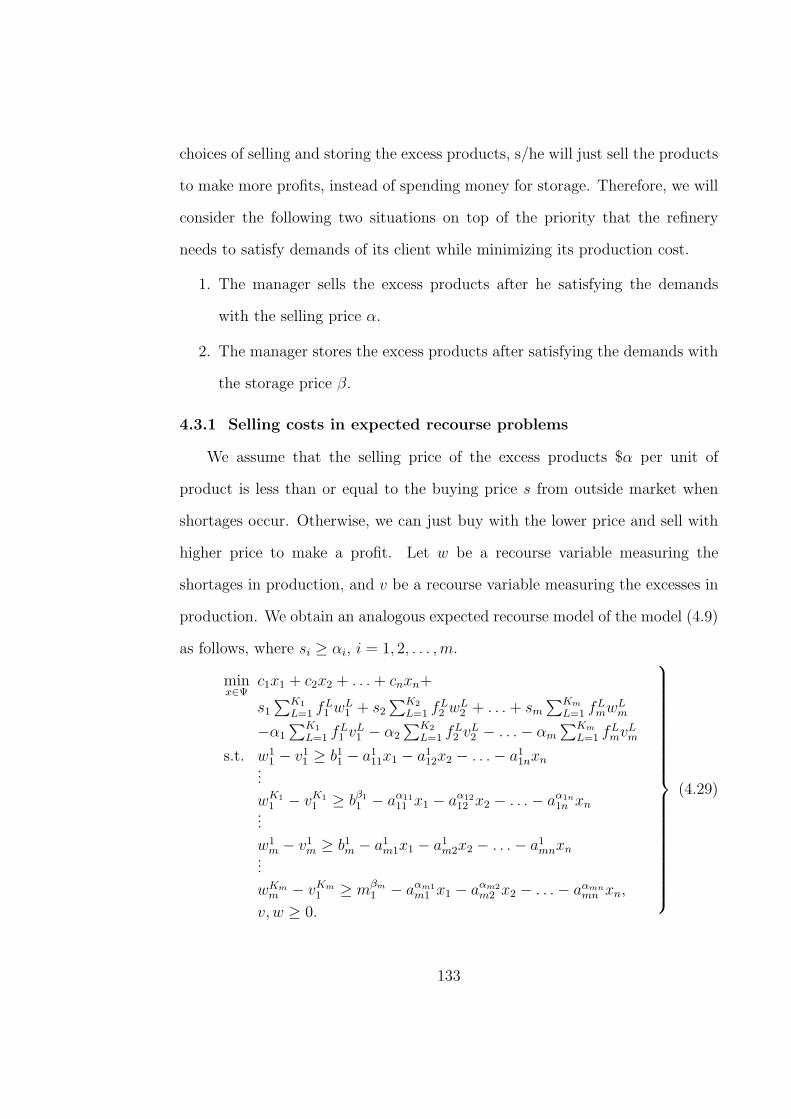
choices of selling and storing the excess products, s/he will just sell the products

to make more profits, instead of spending money for storage. Therefore, we will

consider the following two situations on top of the priority that the refinery

needs to satisfy demands of its client while minimizing its production cost.

1. The manager sells the excess products after he satisfying the demands

with the selling price α.

2. The manager stores the excess products after satisfying the demands with

the storage price β.

4.3.1 Selling costs in expected recourse problems

We assume that the selling price of the excess products $α per unit of

product is less than or equal to the buying price s from outside market when

shortages occur. Otherwise, we can just buy with the lower price and sell with

higher price to make a profit. Let w be a recourse variable measuring the

shortages in production, and v be a recourse variable measuring the excesses in

production. We obtain an analogous expected recourse model of the model (4.9)

as follows, where si ≥ αi, i = 1, 2, . . . ,m.

minx∈Ψ

c1x1 + c2x2 + . . . + cnxn+

s1

∑K1

L=1 fL1 wL

1 + s2

∑K2

L=1 fL2 wL

2 + . . . + sm

∑Km

L=1 fLmwL

m

−α1

∑K1

L=1 fL1 vL

1 − α2

∑K2

L=1 fL2 vL

2 − . . .− αm

∑Km

L=1 fLmvL

m

s.t. w11 − v1

1 ≥ b11 − a1

11x1 − a112x2 − . . .− a1

1nxn...

wK11 − vK1

1 ≥ bβ1

1 − aα1111 x1 − aα12

12 x2 − . . .− aα1n

1n xn...

w1m − v1

m ≥ b1m − a1

m1x1 − a1m2x2 − . . .− a1

mnxn...

wKmm − vKm

1 ≥ mβm

1 − aαm1m1 x1 − aαm2

m2 x2 − . . .− aαmnmn xn,

v, w ≥ 0.

(4.29)

133

The objective function of (4.29) can be rewritten as

c1x1 + c2x2 + . . . + cnxn+

(s1 − α1)

K1∑

L=1

fL1 wL

1 + (s2 − α2)

K2∑

L=1

fL2 wL

2 + . . . + (sm − αm)Km∑

L=1

fLmwL

m

+α1

K1∑

L=1

fL1 (wL

1 − vL1 ) + α2

K2∑

L=1

fL2 (wL

2 − vL2 ) + . . . + αm

Km∑

L=1

fLm(wL

m − vLm).

It is not hard to see that for each i = 1, 2, . . . ,m, wi = (w1i , w

2i , . . . , w

Ki

i ) and

wi − vi = (w1i − v1

i , w2i − v2

i , . . . , wKi

i − vKi

i ) have the same ordering. Hence, we

can apply any of the approaches presented in Sections 4.1 and 4.2 to (4.29).

4.3.2 Storage costs in expected recourse problems

An expected recourse model with recourse variables w and v that represent

the shortages and the storage excesses is

minx∈Ψ

c1x1 + c2x2 + . . . + cnxn+

s1

∑K1

L=1 fL1 wL

1 + s2

∑K2

L=1 fL2 wL

2 + . . . + sm

∑Km

L=1 fLmwL

m

+β1

∑K1

L=1 fL1 vL

1 + β2

∑K2

L=1 fL2 vL

2 + . . . + βm

∑Km

L=1 fLmvL

m

s.t. w11 − v1

1 = b11 − a1

11x1 − a112x2 − . . .− a1

1nxn

...

wK11 − vK1

1 = bβ1

1 − aα1111 x1 − aα12

12 x2 − . . .− aα1n

1n xn

...

w1m − v1

m = b1m − a1

m1x1 − a1m2x2 − . . .− a1

mnxn

...

wKmm − vKm

1 = mβm

1 − aαm1m1 x1 − aαm2

m2 x2 − . . .− aαmnmn xn,

v, w ≥ 0.

(4.30)

The constraints of (4.30) need to be equality constraints. Because at optimal-

ity, if it turns out that wLi − vL

i ≥ bLi − aL

i1x1 − aLi2x2 − . . . − aL

inxn, ∃ i =

134

1, 2, . . . ,m, ∃L = 1, 2, . . . , Ki, while aLi1x1 − aL

i2x2 − . . . − aLinxn > bL

i , then

vLi = 0 would provides the minimum objective value instead of the correct ex-

cess amount vLi = aL

i1x1 − aLi2x2 − . . .− aL

inxn − bLi . An similar argument applies

for the case of ‘≤’.

In order to find a pessimistic, optimistic, and minimax regret solutions for

(4.30), we first rewrite its objective function to

c1x1 + c2x2 + . . . + cnxn +∑K1

L=1 fL1 (s1w

L1 + β1v

L1 )+

∑K2

L=1 fL2 (s2w

L2 + β2v

L2 ) + . . . +

∑Km

L=1 fLm(smwL

m + βmvLm).

Since we do not know the ordering of (siw1i + βiv

1i , siw

2i + βiv

2i , . . . , siw

Ki

i +

βivKi

i ), what we can do is to apply Theorems 2.17 and 2.25 to find all possible

probabilities, as explained in the second paragraph of page 129.

4.4 Comparison between pessimistic, optimistic, minimax regret

approaches and the reviewed approaches

The reviewed approaches in Chapter 3 that incorporate uncertainty informa-

tion into the models are expected recourse, expected average, expected recourse-

average, and interval expected value models. An expected recourse model is for

an LP problem with probability uncertainty. An expected average model is used

when uncertainties in an LP problem with uncertainty are possibility. A mix-

ture of probability and possibility in an LP with uncertainty can be treated by

an expected recourse-average model when these two uncertainties are not in the

same constraint, otherwise we apply an interval expected value model.

However, we had already argued in Chapter 3 that an interval expected

value model is limited in its ability to find the expected objective value in the

135

long run. Moreover, optimal solutions and objective values of an expected av-

erage model and an expected recourse-average model are not reasonable with

respect to the set of probabilities generated by possibility interpretations of un-

certainty. On the other hand, the pessimistic, optimistic and minimax regret

approaches explained in Sections 4.1 and 4.2 are more reasonable and faithful to

the information available. They provide three solutions as information for a user

that in the long run, the user can expect his/her objective value to be between

pessimistic and optimistic values. In addition, the user can use the minimax

solution to minimax the regret of not knowing the actual probability.

Table 4.1 supports the argument made in the previous paragraph that the

reviewed approaches are not reasonable for LP problems with mixed uncertainty.

From the production planning problem in Chapter 3, although an optimal so-

lution (x1, x2) = (45.63, 16.04) for the expected average model is in the ranges

[24.33, 50.33] and [11.33, 37.33] (obtainted from the associated pessimistic and

optimistic models) where the long run solution x1 and x2 is supposed to be, the

objective value z = $139.37 for the expected average model in [$134.67, $160.65]

does not have a reasonable semantic. We may say that there is a probability in

the setM generated by uncertainties presented in (3.13) such that an expected

recourse model with respect to this probability provides the objective value of

$139.37. However, we do not have any theories to support that an optimal first

stage variable solution (x1, x2) obtained by this expected recourse model also is

optimal for the expected average model. Moreover, if we were to use an optimal

solution from the expected average model to represent the LP problem with

possibility uncertainty, we will not have the second stage solution for the con-

136

Table 4.1: Computational Results for the new approaches and the reviewedapproach of the production planning problem.

Types of models, depending upon Raw materials Production costs

uncertainty interpretations x1 x2

1. Expected recourse model 31.80 29.87 $155.38

2. Expected average model 45.63 16.04 $139.37

2.1 Pessimistic expected recourse 24.33 37.33 $160.65

2.2 Optimistic expected recourse 50.33 11 33 $134.67

2.3 Minimax regret of expected recourses 33.15 28.51 R = $17.18

3. Expected recourse-average model 45.63 16.04 $139.37


3.2 Optimistic expected recourse 50.33 11.33 $134.67


4. Interval expected value model [33.89, 44.41] [9.51, 20.03] [$117.35, $127.87]


4.2 Optimistic expected recourse 39.75 21.92 $147.38


137

sequence of the first stage solution. Similar discussion applies for the expected

recourse-average model.

The objective value in the range [$117.35, $127.87] provided by the interval

expected value model is much lower than the optimistic objective value $147.38,

because the interval expected value model does not have any penalty on its

objective function. Moreover, since the probabilities for the expected recourse

model are trapped in the sets of probabilities for the interval expected value

model, an optimal solution and its objective value of the expected recourse

model are in the range of the results from pessimistic and optimistic approaches

associated with the interval expected value model.

We now can handle an LP problem with generalized uncertainty by using the

knowledge from Chapter 2 that each of PC-BRIN interpretations of uncertainty

is in fact a set of probabilities associated with that uncertainty. The uncertainty

in the problem does not have to be limited to probability and possibility. It

can be any PC-BRIN interpretations. The problem can have more than one

interpretation of uncertainty in one constraint. The solutions provide to a user

when we do not know the actual probability of each uncertainty are pessimistic,

optimistic, and minimax regret solutions.

In Chapter 5, we apply the pessimistic, optimistic, and minimax regret

approaches to a farming problem and a radiation shielding design problem.

138

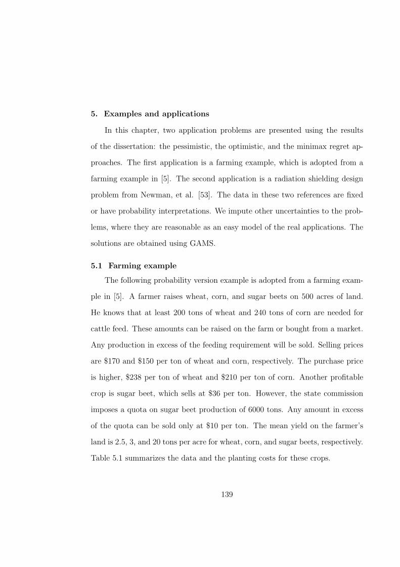
5. Examples and applications

In this chapter, two application problems are presented using the results

of the dissertation: the pessimistic, the optimistic, and the minimax regret ap-

proaches. The first application is a farming example, which is adopted from a

farming example in [5]. The second application is a radiation shielding design

problem from Newman, et al. [53]. The data in these two references are fixed

or have probability interpretations. We impute other uncertainties to the prob-

lems, where they are reasonable as an easy model of the real applications. The

solutions are obtained using GAMS.

5.1 Farming example

The following probability version example is adopted from a farming exam-

ple in [5]. A farmer raises wheat, corn, and sugar beets on 500 acres of land.

He knows that at least 200 tons of wheat and 240 tons of corn are needed for

cattle feed. These amounts can be raised on the farm or bought from a market.

Any production in excess of the feeding requirement will be sold. Selling prices

are $170 and $150 per ton of wheat and corn, respectively. The purchase price

is higher, $238 per ton of wheat and $210 per ton of corn. Another profitable

crop is sugar beet, which sells at $36 per ton. However, the state commission

imposes a quota on sugar beet production of 6000 tons. Any amount in excess

of the quota can be sold only at $10 per ton. The mean yield on the farmer’s

land is 2.5, 3, and 20 tons per acre for wheat, corn, and sugar beets, respectively.

Table 5.1 summarizes the data and the planting costs for these crops.

139

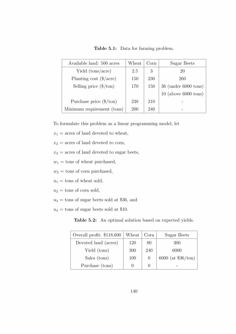
Table 5.1: Data for farming problem.

Available land: 500 acres Wheat Corn Sugar Beets

Yield (tons/acre) 2.5 3 20

Planting cost ($/acre) 150 230 260

Selling price ($/ton) 170 150 36 (under 6000 tons)

10 (above 6000 tons)

Purchase price ($/ton) 238 210 -

Minimum requirement (tons) 200 240 -

To formulate this problem as a linear programming model, let

x1 = acres of land devoted to wheat,

x2 = acres of land devoted to corn,

x3 = acres of land devoted to sugar beets,

w1 = tons of wheat purchased,

w2 = tons of corn purchased,

u1 = tons of wheat sold,

u2 = tons of corn sold,

u3 = tons of sugar beets sold at $36, and

u4 = tons of sugar beets sold at $10.

Table 5.2: An optimal solution based on expected yields.

Overall profit: $118,600 Wheat Corn Sugar Beets

Devoted land (acres) 120 80 300

Yield (tons) 300 240 6000

Sales (tons) 100 0 6000 (at $36/ton)

Purchase (tons) 0 0 -

140

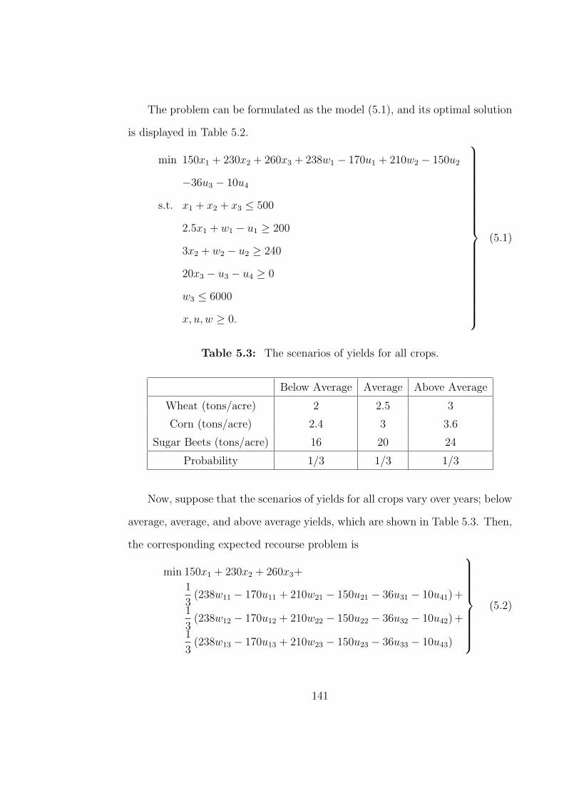
The problem can be formulated as the model (5.1), and its optimal solution

is displayed in Table 5.2.

min 150x1 + 230x2 + 260x3 + 238w1 − 170u1 + 210w2 − 150u2

−36u3 − 10u4

s.t. x1 + x2 + x3 ≤ 500

2.5x1 + w1 − u1 ≥ 200

3x2 + w2 − u2 ≥ 240

20x3 − u3 − u4 ≥ 0

w3 ≤ 6000

x, u, w ≥ 0.

(5.1)

Table 5.3: The scenarios of yields for all crops.

Below Average Average Above Average

Wheat (tons/acre) 2 2.5 3

Corn (tons/acre) 2.4 3 3.6

Sugar Beets (tons/acre) 16 20 24

Probability 1/3 1/3 1/3

Now, suppose that the scenarios of yields for all crops vary over years; below

average, average, and above average yields, which are shown in Table 5.3. Then,

the corresponding expected recourse problem is

min 150x1 + 230x2 + 260x3+

1

3(238w11 − 170u11 + 210w21 − 150u21 − 36u31 − 10u41) +

1

3(238w12 − 170u12 + 210w22 − 150u22 − 36u32 − 10u42) +

1

3(238w13 − 170u13 + 210w23 − 150u23 − 36u33 − 10u43)

(5.2)

141

s.t. 2x1 + w11 − u11 ≥ 200 2.4x2 + w21 − u21 ≥ 240

2.5x1 + w12 − u12 ≥ 200 3x2 + w22 − u22 ≥ 240

3x1 + w13 − u13 ≥ 200 3.6x2 + w23 − u23 ≥ 240

16x3 − u31 − u41 ≥ 0 u31 ≤ 6000

20x3 − u32 − u42 ≥ 0 u32 ≤ 6000

24x3 − u33 − u43 ≥ 0 u33 ≤ 6000

x1 + x2 + x3 ≤ 500 x, u, w ≥ 0.

(5.3)

Table 5.4: An optimal solution based on the expected recourse problem (5.2).

Overall profit: $108,390 Wheat Corn Sugar Beets

Devoted land (acres) 170 80 250

Below Average

Yield (tons) 340 192 4000

Sales (tons) 140 0 4000 (at $36/ton)


Average

Yield (tons) 425 240 5000

Sales (tons) 225 0 5000 (at $36/ton)


Above Average

Yield (tons) 510 288 6000

Sales (tons) 310 48 6000 (at $36/ton)


We assign k = 1, 2, 3 corresponding to the below average, average, and

above average scenarios, respectively. The variables wik, i = 1, 2 refer to the

142

purchase (tons) of crop i at scenario k, when i = 1 is wheat and i = 2 is corn.

Likewise, the variables ujk, j = 1, 2, 3, 4 are the sales (tons) for each scenario.

As an example, u42 represents the amount of sugar beets sold at $10/ton when

yields are average. An optimal solution of the expected recourse problem (5.2)

with the constraints (5.3) is given in Table 5.4. With overall expected profit of

$108,390, the farmer must determined the first stage planting areas of 170, 80,

and 250 acres of wheat, corn, and sugar beets, respectively, before realizing the

crop yields. The yields, sales, and purchases are called the second stage because

they are recovered later after knowing the realization.

5.1.1 A random set version of the farming example

Suppose now that the farmer collects the weather data for the past 300 years

of his town from the local government sources. The farmer finds out that there

are 100 years that have bad weather, but he could not see the pattern when bad

weather may happen. There are 150 years that have no bad things happening

at all; no monster storms, no devastating hail, no outbreak of insects. Besides,

the weather seems to incorporate with the planting schedule during these years.

However, since there are no data of the yields, the farmer does not know for

sure that these 150 years have above average or on average yields. Moreover,

the weather data show that there are 50 years of chaos; mixed good, bad, and

quite days for farming. The farmer cannot decide that these 50 years provide

below average, average, or above average crops’ yields. For this information, the

farmer has a random set with respect to the uncertainty v:

v =

v1 = [2, 2.4, 16]T , v2 = [2.5, 3, 20]T , v3 = [3, 3.6, 24]T

143

such that

m (v1) =1

3, m (v2, v3) =

1

2, m (v1, v2, v3) =

1

6.

We can see that v1 ≤ v2 ≤ v3 and

Bel(v1, v2, v3) = 1, P l(v1, v2, v3) = 1,

Bel(v1, v2) = 13, P l(v1, v2) = 1,

Bel(v1, v3) = 13, P l(v1, v3) = 1,

Bel(v2, v3) = 12, P l(v2, v3) = 2

3,

Bel(v1) = 13, P l(v1) = 1

2,

Bel(v2) = 0, P l(v2) = 23,

Bel(v3) = 0, P l(v3) = 23.

The probabilities (proportions) of below average, average, and above average

yields over 300 years can be in the intervals as follows:

f(v1) ∈

[1

3,1

2

], f(v2) ∈

[0,

2

3

], f(v3) ∈

[0,

2

3

], (5.4)

and therefore,

f(−v1) = 13, f(−v1) = 1

2,

f(−v2) = 0, f(−v2) = 12,

f(−v3) = 23, f(−v3) = 0.

(5.5)

Please note that the proportion f(v1) cannot be continuous on

[1

3,1

2

], it could

be one from

100300

, 101300

, . . . , 150300

. Similar arguments apply for f(v2) and f(v3).

Therefore (5.4) can be written more precisely as

f(v1) ∈

100300

, 101300

, . . . , 150300

,

f(v2) ∈0, 1

300, . . . , 200

300

,

f(v3) ∈0, 1

300, . . . , 200

300

.

(5.6)

144

In this farming problem, we have the excess variables ujk that make the prob-

lem more challenging than the production planning problem in Chapter 4 that

motivated our theories, which has only the shortage variables wik. Next, we

explain that f and f constructed in Theorem 4.2 are still valid to be the proba-

bilities that provide the lowest and highest expected values of the set of expected

recourse problems, respectively.

Given any probability density function f that satisfies (5.6), at an optimality,

we know that

2x∗1 + w∗

11 − u∗11 = 200, 2.4x∗

2 + w∗21 − u∗

21 = 240, 16x∗3 − u∗

31 − u∗41 = 0,

2.5x∗1 + w∗

12 − u∗12 = 200, 3x∗

2 + w∗22 − u∗

22 = 240, 20x∗3 − u∗

32 − u∗42 = 0,

3x∗1 + w∗

13 − u∗13 = 200, 3.6x∗

2 + w∗23 − u∗

23 = 240, 24x∗3 − u∗

33 − u∗43 = 0.

Hence, w∗i3 − u∗

i3 ≤ w∗i2 − u∗

i2 ≤ w∗i1 − u∗

i1, i = 1, 2. The solution can be in these

two forms: w∗ik ≥ 0, u∗

ik = 0 or w∗ik = 0, u∗

ik ≥ 0, i = 1, 2, k = 1, 2, 3. Therefore,

for i = 1, 2,

• w∗i3 ≤ w∗

i2 ≤ w∗i1, and

• −u∗i3 ≤ −u∗

i2 ≤ −u∗i1,

Similarly, −u∗33 − u∗

43 ≤ −u∗32 − u∗

42 ≤ −u∗31 − u∗

41.

• If u∗31 = u∗

32 = u∗33 = 6000, then −u∗

43 ≤ −u∗42 ≤ −u∗

41.

• If u∗31, u

∗32, and u∗

33 are less than 6000, then −u∗43 = −u∗

42 = −u∗41 = 0 and

−u∗33 ≤ −u∗

32 ≤ −u∗31.

145

Hence, all recourse variables are in an increasing order, and we can now apply

Theorem 4.2 to the problem. The expected recourse problems that provide the

lowest and the largest expected objective values are

min(x,u,w)∈Ξ

150x1 + 230x2 + 260x3+

1

3(238w11 − 170u11 + 210w21 − 150u21 − 36u31 − 10u41) +

0 (238w12 − 170u12 + 210w22 − 150u22 − 36u32 − 10u42) +

2

3(238w13 − 170u13 + 210w23 − 150u23 − 36u33 − 10u43)

(5.7)

and

min(x,u,w)∈Ξ

150x1 + 230x2 + 260x3+

1

2(238w11 − 170u11 + 210w21 − 150u21 − 36u31 − 10u41) +

1

2(238w12 − 170u12 + 210w22 − 150u22 − 36u32 − 10u42) +

0 (238w13 − 170u13 + 210w23 − 150u23 − 36u33 − 10u43) ,

(5.8)

where Ξ = (x, u, w) : (x, u, w) satisfies the constraints (5.3). Optimal solu-

tions for these pessimistic and optimistic cases can be seen in Table 5.5.

We also provide an optimal solution based on minimax regret with respect

to not knowing probability of each scenario. For a given probability density

function f , we define

z(f, x, u, w) = 150x1 + 230x2 + 260x3+

f(v1) (238w11 − 170u11 + 210w21 − 150u21 − 36u31 − 10u41) +

f(v2) (238w12 − 170u12 + 210w22 − 150u22 − 36u32 − 10u42) +

f(v3) (238w13 − 170u13 + 210w23 − 150u23 − 36u33 − 10u43) .

This minimax regret of farming problem is stated as

min(x,u,w)∈Ξ

maxf∈M

(χ,υ,ω)∈Ξ

(z (f, x, u, w)− z (f, χ, υ, ω)) , (5.9)

146

Table 5.5: Optimal solutions based on the pessimistic and optimistic expectedrecourse of the farming problem. P = pessimistic, O = optimistic, R = minimaxregret.

Wheat Corn Sugar Beets

P R O P R O P R O

Devoted land

(acres) 100 145.98 183.33 100 82.32 66.67 300 271.70 250

Below Average

Yield (tons) 200 291.95 366.67 240 197.57 160 4800 4347.25 4000

Sales (tons) 0 91.95 166.67 0 0 0 4800 4347.25 4000

Purchase (tons) 0 0 0 0 42.43 80 - - -

Average

Yield (tons) 250 364.94 458.33 300 246.97 200 6000 5434.06 5000

Sales (tons) 50 164.94 258.33 60 6.97 0 6000 5434.06 5000

Purchase (tons) 0 0 0 0 0 40 - - -

Above Average

Yield (tons) 300 437.93 550 360 296.36 240 7200 6520.87 6000

Sales (tons) 100 237.93 350 120 56.36 0 6000 6000 6000

1200∗ 520.87∗

Purchase (tons) 0 0 0 0 0 0 - - -

∗ Sugar beets sold at $10/ton.

Pessimistic profit $87,150

Optimistic profit $127,677.78

Minimax regret value $4656.51

147

where M =f :

∑3i=1 f(vi) = 1 and f satisfies the system (5.6)

, and Ξ =

(x, u, w) : (x, u, w) satisfies the constraints in (5.2). An optimal solution of

the regret problem also is given in Table 5.5.

Therefore, the farmer knows that to maintain the profit of his yields to be

in [$87, 150, $127, 677.78] , he should use his land between 100 and 183.33 acres

for wheat, 66.67 and 100 acres for corn, and 250 and 300 acres for sugar beets.

Moreover, since the farmer does not know the weather in advance, he can use

information that he has about these past 300 years to plan how many acres that

he should use for each crop so that he minimizes the maximum regret of his

decision in the long run. For example, if for some reason, the farmer knows that

the below average, average, and above average years have equal probability of 13,

but he uses the minimax regret strategy instead of Table 5.4. He would regret

no more than $4656.51 in the long run.

148

5.2 An application for radiation shielding design of radiotherapy

treatment vaults

This application problem is based on the real shielding design of radiother-

apy treatment vaults problem that the head of Denver Health’s oncologists,

Francis Newman and his team faced to minimize the cost of their shielding de-

sign. Newman et al. [53] provide three LP problems for minimizing the cost,

the dose of radiation beam, and the thickness of the shielding materials. We will

apply our pessimistic, optimistic, and minimax regret approaches to minimize

the dose of radiation beam beyond the shielding when the costs of shielding

materials are not certain.

A shielding expert wants to optimize the design of shielding, so that the

x-ray dose at the reference point beyond the protective barrier has the lowest

amount. Figure 5.1 illustrates an example of a radiation room with a shielded

wall. The x-ray dose beyond the protective barrier also needs to be lower than

the allowable x-ray dose of 1.0 × 10−4 Sv/week, which is restricted by law.

Newman et al. [53] explain that there are peculiarities of shielding design that

present challenges to his optimization model. Neutrons, in particular, introduce

modeling problems.

To formulate the model, the formula (5.10) outlined in the references [14, 47]

is needed. The barrier transmission for the primary barrier is

Bprimary =(P )(dprimary)

2

(WU)primary(T ), (5.10)

149

where P (Sv/week) = the allowable dose beyond the primary barrier, d (m) =

distance from the x-ray target to the protected point for the primary barrier, W

(Gy/week) = workload, T = occupancy factor, and U = use factor.

Figure 5.1: An example of a radiation room.

Htr is the transmitted x-ray dose beyond a laminated barrier. With a given

Bnew, Htr is computed by replacing P with Htr in Eq.(5.10), and solving for Htr.

To earn Bnew, we need to know the total number ntotal of TV Ls, which can be

obtained from solving the LP problem (5.11). Bnew = 2.7× 10−ntotal .

150

Let TV Lc, TV Ls, and TV Ll be the tenth value layers (the thickness per

TV L) of concrete, steel, and lead, respectively, and let nc, ns, and nl be the num-

ber of TV Ls. ntotal = nc + ns + nl. The number of TV Ls needed for a shielding

design is nB = − log10 B, where B is calculated from Eq. (5.10). Furthermore,

let tdesign be the total barrier thickness allowed for a particular shielding design,

and Ct be the total cost the project can accommodate. Finally, we let cc, cs

and cl be the unit costs ($/square foot/inch of thickness) of concrete, steel, and

lead, respectively. Then, the basic linear programming model minimizing dose

subject to the dose limit (the first row of the constraints), thickness, and cost

constraints is

min−nc − ns − nl

s.t. nc + ns + nl ≥ nB

ccTV Lcnc + csTV Lsns + clTV Lcnl ≤ Ct

ncTV Lc + nsTV Ls + nlTV Ll ≤ tdesign

nc, ns, nl ≥ 0.

(5.11)

Suppose that the costs of concrete, steel, and lead per square foot per 1

inch of thickness are $1, $80, and $200, respectively. We consider a controlled

area and a 15MV beam. The following input data with respect to a 15 MV

beam were used: P = 1.0 × 10−4 Sv/week, Wprimary = 500 Gy/week, T = 1,

Uprimary = 1/4, dprimary = 5m, TV Lc = 0.4246 m = 17 inches, TV Ls = 0.11 m

= 4.33 inches, TV Ll = 0.057 m = 2.24 inches, tdesign = 1.5 m = 60 inches, and

Ct = $1,000/ square foot. Therefore,

B =(1× 10−4)(52)

(500)(1/4)(1)= 2× 10−5 ⇒ nB = − log10(2× 10−5) = 4.7.

151

Using this nB in (5.11), the optimization returns the values nc = 2.847 (1.197

m of concrete), ns = 2.750 (0.303 m of steel), and nl = 0. So, ntotal = 2.847 +

2.750 = 5.597. Hence,

Bnew = 2.7× 10−5.597 = 6.829× 10−6, and

Htr =(500)(1/4)(1)(6.829× 10−6)

52= 3.414× 10−5.

The optimization returns a dose of 3.414 × 10−5 Sv/week, which is 34.14% of

the allowable 1.0× 10−4 Sv/week.

Suppose that the costs of concrete, steel, and lead per inch of thickness are

not uncertain due to the market fluctuations (steel dumping cost, cost of scrap

metal, metal lead mining strikes, etc). The goal is to manage all materials within

the allowable accommodate cost and satisfy the number needed for a shielding

design nB, while minimizing the radiation dose beyond the barrier. Therefore,

we define the second stage variables yc, ys, and yl as the number of TVLs that

need to be reduced so that the total cost for each scenario is still in the given

budget Ct. We hope that with these reductions, we still satisfy the number

needed for a shielding design nB, and the total allowed barrier thickness tdesign.

Otherwise, the recourse model is infeasible.

Suppose that the uncertain cost of concrete per inch of thickness has the

realizations $0.80, $1, and $ 1.20, with the possibility distribution pos(0.80) = 1,

pos(1) = 23, and pos(1.20) = 1. The cost of steel can be $75, $80, or $85 with

probabilities Pr (75) ∈[0, 1

3

], Pr (80) ∈

[23, 1], and Pr (85) ∈

[0, 1

3

],

while the cost of lead are $190 and $200, which have the same probability

Pr (190) = Pr (200) = 12. The possibility distribution provides the ran-

dom set (F ,m) such that m(1) = 23, and m(0.80, 1, 1.20) = 1. Therefore,

152

we obtain the following probability density mass functions:

f (0.80)

c= f

c(0.80) = 1

3, f

(0.80)

c = f c (0.80) = 0,

f (1)

c= f

c(1) = 2

3, f

(1)

c = f c (1) = 23,

f (1.20)

c= f

c(1.20) = 0, f

(1.20)

c = f c (1.20) = 13,

f (75)

s= f

s(75) = 1

3, f

(75)

s = f s (75) = 0,

f (80)

s= f

s(80) = 2

3, f

(80)

s = f s (80) = 23,

f (85)

s= f

s(85) = 0, f

(85)

s = f s (85) = 13,

f (190)

l= f

l(190) = 1

2= f l (190) = f

(190)

l , and

f (200)

l= f

l(200) = 1

2= f l (200) = f

(200)

l .

These uncertainties could happen because of various situations. For example,

Company A sets the concrete’s price according to the following three cases: case

1, case 2, and case 3 as $0.8 , $1, and $ 1.20 per inch of thickness of concrete,

respectively. It provides information about the availability of these three cases

as that at least one of case 1 or case 3 is available1

3of the time, and

2

3of the

time, either case 1, case 2, or case 3 is available. Company B, who delivers steel,

also sets the steel’s price according to the other three cases: case 1′(cost $75) is

available less than1

3of the time, case 2

′(cost $85) is available less than

1

3of

the time, and case 3′(cost $80) is available more than

2

3of the time. Finally,

each of two cases that company C uses for pricing lead is available1

2of the time.

Therefore, we have the uncertainty information as stated at the beginning of the

paragraph.

We transform the problem (5.11) to the following expected recourse problem,

where f can be replaced by f and f .

153

min −nc − ns − nl + f(0.80)c f

(75)s f

(190)l

(y

(0.80)c + y

(75)s + y

(190)l

)+ . . .+

f(1.20)c f

(85)s f

(200)l

(y

(1.20)c + y

(85)s + y

(200)l

)

s.t. nc, ns, nl, yc, ys, yl ≥ 0,

nc − y(0.80)c + ns − y

(75)s + nl − y

(190)l ≥ nB,

nc − y(0.80)c + ns − y

(75)s + nl − y

(200)l ≥ nB,

...

nc − y(1.20)c + ns − y

(85)s + nl − y

(200)l ≥ nB,

0.80TV Lc(nc − y(0.80)c ) + 75TV Ls(ns − y

(75)s ) + 190TV Ll(nl − y

(190)l ) ≤ Ct,

1TV Lc(nc − y(1)c ) + 80TV Ls(ns − y

(80)s ) + 200TV Ll(nl − y

(200)l ) ≤ Ct,

...

1.20TV Lc(nc − y(1.20)c ) + 85TV Ls(ns − y

(85)s ) + 200TV Ll(nl − y

(200)l ) ≤ Ct,

(nc − y(0.80)c )TV Lc + (ns − y

(75)s )TV Ls + (nl − y

(190)l )TV Ll ≤ tdesign,

(nc − y(0.80)c )TV Lc + (ns − y

(75)s )TV Ls + (nl − y

(200)l )TV Ll ≤ tdesign,

...

(nc − y(1.20)c )TV Lc + (ns − y

(85)s )TV Ls + (nl − y

(200)l )TV Ll ≤ tdesign.

The objective function can be rewritten as

min−nc − ns − nl + f(0.80)c y

(0.80)c + f

(1)c y

(1)c + f

(1.20)c y

(1.20)c +

f(75)s y

(75)s + f

(80)s y

(80)s + f

(85)s y

(85)s + f

(190)l y

(190)l + f

(200)l y

(200)l .

(5.12)

An optimal solution of the expected recourse problem with f provides nc =

2.8294, ns = 2.9332, y(1.20)c = 0.7185, y

(80)s = 0.1833, y

(85)s = 0.3451, and the

other variables are zero. The objective value with respect to f is -5.6404. Hence,

the optimization returns the average values nc = 2.8294− 13·0− 2

3·0−0·0.7185 =

2.8294 (1.20 m of concrete), and ns = 2.9332− 13·0− 2

3·0.1833 −0·0.3451 = 2.811

154

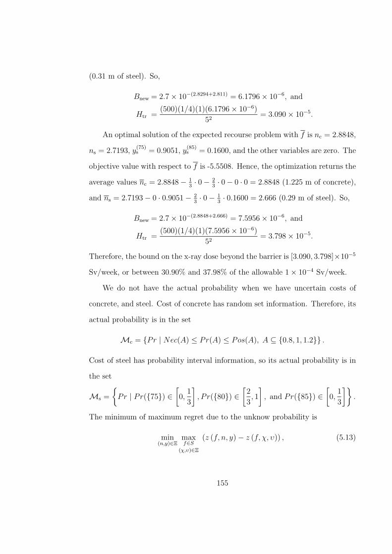
(0.31 m of steel). So,

Bnew = 2.7× 10−(2.8294+2.811) = 6.1796× 10−6, and

Htr =(500)(1/4)(1)(6.1796× 10−6)

52= 3.090× 10−5.

An optimal solution of the expected recourse problem with f is nc = 2.8848,

ns = 2.7193, y(75)s = 0.9051, y

(85)s = 0.1600, and the other variables are zero. The

objective value with respect to f is -5.5508. Hence, the optimization returns the

average values nc = 2.8848− 13· 0− 2

3· 0− 0 · 0 = 2.8848 (1.225 m of concrete),

and ns = 2.7193− 0 · 0.9051− 23· 0− 1

3· 0.1600 = 2.666 (0.29 m of steel). So,

Bnew = 2.7× 10−(2.8848+2.666) = 7.5956× 10−6, and

Htr =(500)(1/4)(1)(7.5956× 10−6)

52= 3.798× 10−5.

Therefore, the bound on the x-ray dose beyond the barrier is [3.090, 3.798]×10−5

Sv/week, or between 30.90% and 37.98% of the allowable 1× 10−4 Sv/week.

We do not have the actual probability when we have uncertain costs of

concrete, and steel. Cost of concrete has random set information. Therefore, its

actual probability is in the set

Mc = Pr | Nec(A) ≤ Pr(A) ≤ Pos(A), A ⊆ 0.8, 1, 1.2 .

Cost of steel has probability interval information, so its actual probability is in

the set

Ms =

Pr | Pr(75) ∈

[0,

1

3

], P r(80) ∈

[2

3, 1

], and Pr(85) ∈

[0,

1

3

].

The minimum of maximum regret due to the unknow probability is

min(n,y)∈Ξ

maxf∈S

(χ,υ)∈Ξ

(z (f, n, y)− z (f, χ, υ)) , (5.13)

155

where, Ξ = (n, y) | (n, y) satisfies the constraints in (5.12) ,

S =

f = (fc, fs, fl) | fc ∈Mc, fs ∈Ms, and f(190)l = f

(200)l = 1

2

, and

z (f, n, y) =−nc − ns − nl + f(0.80)c y

(0.80)c + f

(1)c y

(1)c + f

(1.20)c y

(1.20)c +

f(75)s y

(75)s + f

(80)s y

(80)s + f

(85)s y

(85)s + f

(190)l y

(190)l + f

(200)l y

(200)l .

Applying the minimax regret procedure to the problem (5.13), the minimum of

the maximum regret is 0.0296, when nc∗ = 2.8717, ns∗ = 2.7699, y(1.20)c∗ = 0.0624,

y(80)s∗ = 0.0462, y

(85)s∗ = 0.2064, and the other variables are zero. No matter what

probability in S that we pick to represent the uncertainty, we will not regret

more than 0.0296 of total number of TV Ls with this solution (n∗, y∗).

However, for the safety, any person who does not want to get exposed to

the radiation would want to know the highest number of the x-ray dose beyond

the barrier. Therefore, we may provide the pessimistic solution, which will tells

that it is not more than 3.798 × 10−5 Sv/week on average of the x-ray dose

beyond the barrier. If we were to use the minimax regret solution to represent

the problem, then the pessimistic and the optimistic amount of the x-ray dose

beyond the barrier with respect to this minimax regret solution will 4.0657×10−5

and 3.3078× 10−5 Sv/week, which are 33.08% and 40.66% of the allowale dose.

These percentage numbers are shifted from the actual numbers 30.90% and

37.98% by at most 3%.

Some people who are concerned about the extreme scenario that provides

the highest dose beyond the barrier may not use the expected recourse approach,

but instead use cc = $1.20, cs = $85, and cl = $200 in (5.11), which will result

5.6148 × 10−5 Sv/week of the x-ray dose beyond the barrier, or 56.15% of the

allowable by law, by using nc = 2.8240 and ns = 2.5570.

156

We include all the solutions obtained in this section in Table 5.6, for an easy

reading.

Table 5.6: A pessimistic, an optimistic, a minimax regret, and an extremescenario solution for the radiation shielding design problem.

Average number of Pessimistic solution Optimistic solution

TV Ls

Concrete (nc) 2.8848 2.8294

(122.50 cm of concrete) (120.14 cm of concrete)

Steel (ns) 2.6660 2.8110

(29 cm of concrete) (31 cm of steel)

X-ray dose beyond 3.798× 10−5 3.090× 10−5

the barrier (Sv/week) (37.98%) (30.90%)

Number of TV Ls Minimax regret Extreme scenario

solution solution

Concrete (nc) 2.8717 2.8240

(122 cm of concrete) (119.90 cm of concrete)

Steel (ns) 2.7699 2.5570

(30.47 cm of steel) (28.13 cm of steel)

X-ray dose beyond [3.3078, 4.0657]× 10−5 5.6148× 10−5

the barrier (Sv/week) ([33.08%, 40.66%]) (56.15%)

157

6. Conclusion

The dissertation has developed linear programming problems with coeffi-

cients whose uncertainies are restricted to a finite set of realizations. The uncer-

tainties in the scope of this dissertation have had PC-BRIN interpretations. We

explained in Chapter 2 that each of PC-BRIN interpretations of uncertainty can

be written as a set of probability measuresM associated with that uncertainty.

When an uncertainty u has random set interpretation (or other interpretations

that can be written as a random set, see Figure 2.7), we have proved that any

probability in the set of probability measures associated with this random set is

trapped between belief and plausibility functions.

Two density functions for the lowest and highest expected values of u (or

an evaluation function of U , where U is the set of all finite realizations of u) can

be constructed by Theorem 2.17, when u has random set interpretation. These

constructed density functions use fewer calculations than the process of estab-

lishing an associated LP problems for finding the lowest and highest expected

values of this random set uncertainty. Theorem 2.25 and Corollary 2.26 handle

the IVPM case.

Theorems 2.17 and 2.25 are used in the proof of remodeling pessimistic and

optimistic recourse problems as linear programs. The theorems also are used to

tackle the relaxation procedure for a minimax regret of expected recourse mod-

els. We apply these theorems with reduced expected recourse models which have

much smaller size of variables and constraints than ordinary expected recourse

158

models.

A pessimistic, an optimistic, and a minimax regret of expected recourse

models are introduced to be able to handle an LP problem with generalized

uncertainty, where more than one uncertainty interpretation can be in the same

constraint. Therefore, we overcome the limitation of all approaches in literature.

Since we do not know the actual probability of uncertainty, the three solution

approaches provided by this thesis are useful information for a user. The user

will have extended knowledge about the consequences of various decisions and

associated costs in the long run that will be between the pessimistic and the

optimistic solution. The minimax regret approach of a set of expected recourse

models also is a reasonable solution when we want to see a solution that mini-

mizes the maximum regret of not knowing the actual probability.

This dissertation focused on uncertainty over a finite case. However, we

have some results that could apply to continuous realizations of uncertainty,

and the full development of these ideas to the continuous case is a logical next

step. Moreover, the penalty price also could be uncertain, which means that

an expected recourse model becomes a nonlinear program, and the developed

theorems may no longer apply.

In addition to this research, we should find the computational complexity

of all three approaches and compare them with an expected recourse model, to

see how much harder than the computation of a single expected recourse model

we need to work on. Hence, we can compare our approaches with a simulation

approach. We may randomly choose a probability in the set of probabilitiesM,

use it in an expected recourse model, re-do the process of choosing a proba-

159

bility and finding its associated expected recourse solution for a large number

of iterations. We would see an approximated pessimistic and an approximated

optimistic objective value.

We expect that an expected recourse solution whose associated probability

belongs to set M is trapped between a pessimistic and an optimistic solution.

We also should check that a minimax regret solution is trapped between a pes-

simistic and an optimistic solution, in general. It may have a nice structure

that helps reduce the size of the density functions in Algorithm 4.6, so that the

complexity of the relaxation procedure is improved. We may apply the idea of

using duality and complementarity slackness to the relaxation procedure when

an LP’s objective coefficients belong to M. Moreover, we may write a gen-

eral code in MATLAB (or other programming languages) for LP problems with

generalized uncertainty.

Lastly, another direction is to find an extension to the expected average ap-

proach so that its solution not only provides a richer semantic but also guarantees

to lie within the bounds of associated pessimistic and optimistic solutions.

160

APPENDIX A. How to obtain a basic probability assignment

function m from a given belief measure Bel

The materials in this Appendix can be found in Shafer [60].

Theorem A.1 Suppose U is a finite set and Bel and m are a belief measure,

and a basic probability assignment function on P(U), respectively. Then

m(A) =∑

B|B⊆A

(−1)|A−B|Bel(B),

for all A ⊆ X.

We need the following lemmas in order to solve Theorem A.1.

Lemma A.2 If A is a finite set, then

∑

B⊆A

(−1)|B| =

1 if A = ∅,

0 otherwise.

Proof: We know that for a positive number n,

(n0

)−

(n1

)+

(n2

)+ . . . + (−1)n

(n0

)= (1− 1)n = 0.

So, whenever A = θ1, θ2, . . . , θn is a finite non-empty set,

∑

B⊆A

(−1)|B| = (−1)|∅| +∑

i

(−1) |θi|+∑

i<j

(−1) |θi, θj|+ . . . + (−1)|A|

=

(n0

)−

(n1

)+

(n2

)+ . . . + (−1)n

(n0

)= (1− 1)n = 0.

161

And when A = ∅,

∑

B⊆A

(−1)|B| = (−1)|A| = (−1)0 = 1.

Lemma A.3 If A is a finite set and B ⊆ A, then

∑

CB⊆C⊆A

(−1)|C| =

(−1)|A| if A = B,

0 otherwise.

Proof: This lemma is seen to follow from Lemma A.2 once it is noticed that

∑

CB⊆C⊆A

(−1)|C| =∑

D⊆A−B

(−1)|B∪D| = (−1)|B|∑

D⊆A−B

(−1)|D|.

Proof of Theorem A.1

We know that Bel(A) =∑

B⊆A

m(B). So,

∑

B⊆A

(−1)|A−B|Bel(B) = (−1)|A|∑

B⊆A

(−1)|B|Bel(B)

= (−1)|A|∑

B⊆A

(−1)|B|∑

C⊆B

m(C)

= (−1)|A|∑

C⊆A

m(C)∑

BC⊆B⊆A

(−1)|B|

= (−1)|A|m(A)(−1)|A|

= m(A).

162

APPENDIX B. The nestedness requirement of focal elements for a

possibility measure

The requirement that focal elements be nested restricts belief and plausibil-

ity measures to necessity and possibility measures. Theorem B.1 can be found

in Chapter 7 of [28].

Theorem B.1 Let a given finite body of evidence (F ,m) be nested. Then, the

associated belief and plausibility measures have the following properties for all

A,B ∈ P(U) :

(a) Bel(A ∩B) = min [Bel(A), Bel(B)];

(b) Pl(A ∪B) = max [Pl(A), P l(B)].

Proof:

(a) Since the focal elements in (F ) are nested, they may be linearly ordered

by the subset relationship. Let F = A1, A2, . . . , An, and assume that

Ai ⊂ Aj whenever i < j. Consider now arbitrary subsets A and B of

U . Let i1 be the largest integer i such that Ai ⊆ A, and let i2 be the

largest integer i such that Ai ⊆ B. Then, Ai ⊆ A and Ai ⊆ B if and only

if i ≤ i1 and i ≤ i2, respectively. Moreover, Ai ⊆ A ∩ B if and only if

i ≤ min(i1, i2). Hence,

Bel(A ∩B) =

min(i1,i2)∑

i=1

m(Ai) = min

[i1∑

i=1

m(Ai),

i2∑

i=1

m(Ai)

]

= min [Bel(A), Bel(B)] .

163

(b) Assume that (a) holds. Then, using Pl(A) = 1 − Bel(Ac) for all A,B ∈

P(U), we have

Pl(A ∪B) = 1−Bel ((A ∪B)c)

= 1−Bel (Ac ∩Bc)

= 1−min [Bel(Ac), Bel(Bc)]

= max [1−Bel(Ac), 1−Bel (Bc)]

= max [Pl(A), P l(B)] .

Therefore, we have the properties for possibility and necessity measures:

(a′) Nec(A ∩B) = min [Nec(A), Nec(B)];

(b′) Pos(A ∪B) = max [Pos(A), Pos(B)].

We can prove the converse statement of Theorem B.1.

Theorem B.2 If for all A,B ∈ P(U), we have

(a) Bel(A ∩B) = min [Bel(A), Bel(B)], or

(b) Pl(A ∪B) = max [Pl(A), P l(B)],

then the focal elements are nested.

Proof: The proof is based on having information (b). (We can derive (a) from

(b)). Let U = u1, u2, . . . , un. Suppose that U can be partitioned into k sets

for some k ≤ n as follows:

U0 =u0 | Pl(

u0) = 1

,

U1 =u1 | Pl(

u1) = a1 < 1

,

164

U2 =u2 | Pl(

u2) = a2 < a1

,

...

Uk =uk | Pl(

uk) = ak < ak−1

.

Let A0 ( U0, and A0 6= ∅. For any u ∈k⋃

i=1

U i, we have 1 = Pl (U\A0) =

max [Pl (U\ (A0 ∪ u)) , P l (u)]. Since Pl (u) < 1,

1 = Pl(U\(A0 ∪ u

))= 1−Bel

(A0 ∪ u

)= 1−

∑m(B)

B⊆(A0∪u)

⇒∑

m(B)B⊆(A0∪u)

= 0.

Thus, for ki = |U i|, we achieve

• m(ui) = 0, ∀ i = 1, 2, . . . , n,

• m(u0

i , u0j

) = 0, ∀ i, j = 1, 2, . . . , k0, and

m(u0

i , u1j

) = 0, ∀ i = 1, 2, . . . , k0, j = 1, 2, . . . , k1,

• m(u0

i , u0j , u

0k,) = 0, ∀ i, j, k = 1, 2, . . . , k0, and

m(u0

i , u0j , u

1k

) = 0, ∀ i, j = 1, 2, . . . , k0, k = 1, 2, . . . , k1,

...

• m(A0i ) = 0, where A0

i = U0\ u0i , ∀ i = 1, 2, . . . , k0, and

m((

A0i \u0

j

)∪ u1

k)

= 0, ∀ i, j = 1, 2, . . . , k0, k = 1, 2, . . . , k1,

• m(A0

i ∪u1

j

)= 0, ∀ i = 1, 2, . . . , k0, j = 1, 2, . . . , k1.

We also know that 1 > Pl (U\U0) = 1 − Bel (U0). Hence, 0 < Bel (U0) =∑

B⊆U0

m(B) < 1. Since m(B) = 0, ∀B ( U0 (as listed above), Bel (U0) =

m(U0), and 0 < m(U0) < 1. We achieve the first focal element as the set U0.

We expect that other focal elements will contain U0.

165

Pl (U\U0) = Pl(U1∪U2∪ . . .∪Uk) = 1−m(U0) means that a1 = Pl(U1) =

1−m(U0). For every A1 ( U1, and A1 6= ∅, we have 1−m(U0) = a1 = Pl(A1) =

1−Bel(U\A1), which implies that m(U0) = Bel(U\A1) =∑

B⊆(U\A1)

m(B). Hence,

we have m(B) = 0, ∀B 6= U0, such that B ⊆ (U\A1), ∀A1 ( U1, A1 6= ∅. We

also know that 1−m(U0) > Pl(U\(U0 ∪U1))) = 1−Bel(U0 ∪U1)⇒ m(U0) <

Bel(U0 ∪ U1) =∑

B⊆(U0∪U1)

m(B). But, m(B) = 0,∀ B ⊆ U0 ∪ U1, B 6= U0, B 6=

U0∪U1. Therefore, m(U0∪U1) > 0. The second focal element is the set U0∪U1.

Bel(U0 ∪ U1) = m(U0) + m(U0 ∪ U1).

The next focal element is2∑

i=0

U i. Here is the reason. a2 = Pl(U\(U0∪U1)) =

1−Bel(U0∪U1) = 1−m(U0)−m(U0∪U1) For every A2 ( U2, and A2 6= ∅, we

have 1−m(U0)−m(U0∪U1) = a2 = Pl(A2) = 1−Bel(U\A2), which implies that

m(U0) + m(U0 ∪ U1) = Bel(U\A2) =∑

B⊆(U\A2)

m(B). Hence, we have m(B) =

0, ∀B 6= U0, B 6= (U0 ∪U1) such that B ⊆ (U\A2), ∀A2 ( U2, A2 6= ∅. We also

know that 1−m(U0)−m(U0 ∪ U1) > Pl(U\(U0 ∪ U1 ∪ U2))) = 1− Bel(U0 ∪

U1 ∪ U2) ⇒ m(U0) + m(U0 ∪ U1) < Bel(U0 ∪ U1 ∪ U2) =∑

B⊆(U0∪U1∪U2)

m(B).

But, m(B) = 0,∀ B ⊆ U0 ∪ U1 ∪ U2, B 6= U0, B 6= U0 ∪ U1, B 6=2∑

i=0

U i.

Therefore, m(U0∪U1∪U2) > 0. The third focal element is the set U0∪U1∪U2.

Bel(U0 ∪ U1 ∪ U2) = m(U0) + m(U0 ∪ U1) + m(U1 ∪ U1 ∪ U2).

Follow the similar pattern as in the previous two paragraphs, we can con-

clude that

F =

U0,

1∑

i=0

U i,2∑

i=0

U i, . . . ,k∑

i=0

U i = U

.

166

REFERENCES

[1] H. Aissi, C. Bazgan, and D. Vanderpooten. Min-max and min-max re-gret versions of combinatorial optimization problems: A survey. EuropeanJournal of Operational Research, 197(2):427–238, 2009.

[2] R. Banuelos. Measure Theory and Probability. Department of Mathematics,Purdue University, 2003. Lecture notes.

[3] M.S. Bazaraa, J. J. Jarvis, and H. D. Sherali. Linear Programming andNetwork Flows. John Wiley & Sons, Inc, Canada, 2 edition, 1990.

[4] R. E. Bellman and L. A. Zadeh. Decision-making in a fuzzy environment.Management Sci., Serial B 17:141–164, 1970.

[5] J. R. Brige and F. Louveaux. Introduction to Stochastic Programming.Springer, 1997.

[6] C. Carlsson and R. Fuller. On possibilistic mean value and variance of fuzzynumbers. Fuzzy Sets and Systems, (122):315–326, 2001.

[7] G. B. Dantzig. Linear Programming and Extensions. Princeton UniversityPress, Princeton, 1963.

[8] L. M. de Campos, J. F. Huete, and S. Moral. Probability intervals: A toolfor uncertain reasoning. International Journal of Uncertainty, Fuzzinessand Knowledge-Based Systems, 2(2):167–196, 1994.

[9] A. P. Dempster. Upper and lower probability induced by a multivaluedmapping. Annals of Mathematical Statistics, 38:325–339, 1967.

[10] S. Destercke, D. Dubois, and E. Chojnacki. Unifying practical uncertaintyrepresentations: I. generalized p-boxes. International Journal of Approxi-mate Reasoning, 49:649–663, 2008.

[11] S. Destercke, D. Dubois, and E. Chojnacki. Unifying practical uncertaintyrepresentations: II. clouds. International Journal of Approximate Reason-ing, 49:664–677, 2008.

167

[12] D. Dubois and H. Prade. Systems of linear fuzzy constraints. Fuzzy Setsand Systems, (3):37–48, 1980.

[13] Didier Dubois and Henri Prade. Random sets and fuzzy interval analysis.Fuzzy Sets and Systems, (42):87–101, 1991.

[14] J. A. Dye, J. E. Rodgers, R. K. Wu, P. J. Biggs, P. H. McGinley, and R. M.McCall. Recommendations of the National Council on Radiation Protectionand Measurements, Structural Shielding Design and Evaluation for Mega-voltage X- and Gamma-Ray Radio-therapy Facilities. NCRP Report No.151, Bethesda, MD, 2005.

[15] L. Dymowa and M. Dolata. The transportation problem under probabilisticand fuzzy uncertainties. http://zsiie.icis.pcz.pl/artykuly/md/md_

wrodaw.pdf.

[16] Th. Fetz and M. Oberguggenberger. Propagation of uncertainty throughmultivariate functions in the framwork of sets of probability measures. Re-liability Engineering & System Safety, (85):73–87, 2004.

[17] M. Fiedler, J. Nedoma, J. Ramik, J. Rohn, and K. Zimmermann. LinearOptimization Problems with Inexact Data. Springer, 2006.

[18] T. Gal and J. Nedoma. Multiparametric linear programming. ManagementScience, (18):406–422, 1972.

[19] D. M. Gay. Solving interval linear equations. SIAM J. Number Anal.,19(4):858–870, 1982.

[20] M. Inuiguchi, H. Ichihashi, and H. Tanaka. Stochastic versus fuzzy ap-proaches to multi-objective mathematical programming under uncertainty.In R. Slowinski and J. Teghem, editors, Fuzzy Programming: A Survey ofRecent Developments, pages 45–68. Kluwer Academic Publishers, 1990.

[21] M. Inuiguchi and M. Sawaka. Minimax regret solution to linear program-ming problems with an interval objective function. European Journal ofOperational Research, (86):526–536, 1995.

[22] M. Inuiguchi and M. Sawaka. Minimax regret analysis in linear programswith an interval objective function. In Proceedings of IWSCI’96, pages308–317. IEEE, 1996.

168

[23] M. Inuiguchi, T. Tanino, and M. Sakawa. Membership function elicitationin possibilistic programming problems. Fuzzy Sets and Systems, (111):29–45, 2000.

[24] K. D. Jamison. Modeling uncertainty using probabilistic based possibilitytheory with applications to optimization. PhD thesis, Department of Math-ematics, University of Colorado at Denver, Denver, CO, 1998.

[25] K.D. Jamison and W. A. Lodwick. The construction of consistent possibil-ity and necessity measures. Fuzzy Set and Systems, 132:1–10, 2002.

[26] P. Kall and S. W. Wallace. Stochastic Programming. John Wiley & Sons,Inc, 1994.

[27] G. J. Klir. Is there more to uncertainty than some probability theoristsmight have us believe? Int. J. General Systems, 15:347–378, 1989.

[28] G.J. Klir and Bo Yuan. Fuzzy Sets and Fuzzy Logic: Theory and Applica-tions. Prentic Hall P T R, New Jersey, 1995.

[29] R. Krawczyk. Interval mathematics. In Lecture Notes in Computer Science29, pages 215–222. Springer Verlag, New York, 1975.

[30] K. K. Lai et al. A class of linear interval programming problems and itsapplication to portfolio selection. IEEE Transactions on Fuzzy Systems,10(6):698–703, 2002.

[31] J. F. Lemmer and H. E. Kyburg Jr. Conditions for the existence of belieffunctions corresponding to intervals of belief. In AAAI-91 Proceedings,pages 488–493. AAAI, 1991.

[32] Y. P. Li, G. H. Huang, H. N. Xiao, and X.S. Qin. Municipal solid wastemanagement under uncertainty: an interval-fuzzy two-stage stochastic pro-gramming approach. Environmental Informatics Archives, 5:131–145, 2007.

[33] Baoding Liu. Uncertain Programming. John Wiley & Sons, Inc, New York,2000.

[34] W. A. Lodwick. Analysis of structure in fuzzy linear programs. Fuzzy Setsand Systems, (38):15–26, 1990.

[35] W. A. Lodwick and K. A. Bachman. Solving large-scale fuzzy and possi-bilistic optimization problems. Fuzzy Optimization and Decision Making,4:258–275, 2005.

169

[36] W. A. Lodwick and K. D. Jamison. Interval valued probability in the anal-ysis of problems containing a mixture of possibilistic, probabilistic and in-terval uncertainty. In Fuzzy Information Processing Society, 2006. NAFIPS2006. Annual Meeting of the North American, pages 617–620. IEEE, 2006.

[37] W. A. Lodwick and K. D. Jamison. Theoretical and semantic distinctionsof fuzzy, possibilistic, and mixed fuzzy/possibilistic optimization. FuzzySets and Systems, (158):1861–1872, 2007.

[38] W. A. Lodwick and K. D. Jamison. The use of interval-valued probabilitymeasures in optimization under uncertainty for problems containing a mix-

ture of fuzzy, possibility and interval uncertainty. In Proceedings of the 12th

International Fuzzy Systems Association World Congress on Foundation ofFuzzy Logic and Soft Computing, Lecture Notes In Artificial Intelligence,pages 361–370, 2007.

[39] W. A. Lodwick and Elizabeth Untiedt. Introduction to Fuzzy and Possi-bilistic Optimization. Department of Mathematics, University of Coloradoat Denver, September 9, 2009. Monograph Draft.

[40] D. G. Luenberger. Linear and Nonlinear Programming. Springer, 2 edition,2003.

[41] Chr. Mandl. Number of operations for updating the elimination form ofthe basis-inverse of the revised simplex algorithm. Computing, 18:365–366,1977.

[42] I. Maqsood, G. H. Huang, and J. S. Yeomans. An interval-parameter fuzzytwo-stage stochastic program for water resources management under uncer-tainty. European Journal of Operational Research, 167:208–225, 2005.

[43] Diego Marın Andres Alvarez. Infinite random sets and applications inuncertainty analysis. PhD thesis, The Fakultat fur Bauingenieurwis-senschaften of the Leopold-Franzens Universitat Innsbruck, 2007.

[44] H. E. Mausser. Minimizing maximum regret for linear programs with inter-val objective function coefficients. PhD thesis, Graduate School of Business,University of Colorado, Boulder, CO, 1997.

[45] H. E. Mausser and M. Laguna. A new mixed integer formulation for themaximum regret problem. International Transactions in Operational Re-search, 5(5):389–403, 1998.

170

[46] H. E. Mausser and M.Laguna. A heuristic to minimax absolute regretfor linear programs with interval objective function coefficients. EuropeanJournal of Operational Research, (117):157–174, 1999.

[47] P. H. McGinley. Shielding techniques for radiation oncology facilities. Med-ical Physics Pub, Madison, WI, second edition, 2002.

[48] R. E. Moore. Methods and Applications of Interval Analysis. SIAM,Philadelphia, 1979.

[49] T. Morrison and H. J. Greenberg. Robust optimization. In A. R. Ravin-dran, editor, Operations Research and Management Science Handbook, TheOperations Research Series, chapter 14. CRC Press, Boca Raton, FL, 2008.

[50] S. G. Nash and A. Sofer. Linear and Nonlinear Programming. TheMcGraw-Hill Companies, Inc., New York, 1996.

[51] A. Neumaier. On the structure of clouds. http://www.mat.univie.ac.

at/~neum/papers.html. 05/06/2010.

[52] A. Neumaier. Clouds, fuzzy sets and probability intervals. Reliable Com-puting, 4(10):249–272, 2004.

[53] F. Newman and M. Asadi-Zeydabadi. An optimization model and solutionfor radiation shielding design of radiotherapy treatment vaults. AmericanAssociation of Physicists in Medicine, 35(1):171–180, 2008.

[54] Hung T. Nguyen. An Introduction to Random Sets. Chapman & Hall/CRC,Boca Raton, FL, 2006.

[55] M. Oberguggenberger. The mathematics of uncertainty: models, methodsand interpretations. In Analyzing Uncertainty in Civil Engineering, pages51–72. Springer Berlin Aeidelberg, 2005.

[56] M. Oberguggenberger and W. Fellin. Reliability bounds through randomsets: non-parametric methods and geotechnical applications. Computers &Structures, 86:1093–1101, 2008.

[57] J. Ramik and J. Rimanek. Inequality relation between fuzzy numbers andits use in fuzzy optimization. Fuzzy Sets and Systems, 16(2):123–138, 1985.

[58] J. Rohn. Solvability of systems of linear interval equations. SIAM J. MatrixAnal. Appl., 25(1):237–245, 2003.

171

[59] Sheldon Ross. A First Course in Probability. Prentice Hall, Upper SaddleRiver, New Jersey, 1997.

[60] G. Shafer. A Mathematical Theory of Evidence. Princeton University Press,Princeton, New Jersey, 1976.

[61] G.J. Shih and R. A. S. Wangsawidjaja. Mixed fuzzy-probabilistic program-ming approach for multiobjective engineering optimization with randomvariables. Computer & Structures, 59(2):283–290, 1996.

[62] K. Shimizu and E. Aiyoshi. Necessary conditions for min-max problems andalgorithms by a relaxation procedure. IEEE Transactions on AutomaticControl, AC-25(1):62–66, February 1980.

[63] R. E. Steuer. Algorithms for linear programming problems with inter-val objective function coefficients. Mathematics of Operations Research,6(3):333–348, August 1981.

[64] H. Tanaka and K. Asai. Fuzzy linear programming with fuzzy numbers.Fuzzy Sets and Systems, (13):1–10, 1984.

[65] H. Tanaka, H. Ichahashi, and K. Asai. A formulation of fuzzy linear pro-gramming problem based on comparison of fuzzy numbers. Control andCybernetics, 3(13), 1984.

[66] H. Tanaka, H. Ichihashi, and K. Asai. Fuzzy decision in linear programmingwith trapezoid fuzzy parameters. In J. Kacpryzk and R. R. Yager, editors,Management Decision Support Systems Using Fuzzy Sets and PossibilityTheory. Verlag TUV, Koln, 1985.

[67] H. Tanaka, T. Okuda, and K. Asia. On fuzzy mathematical programming.Trans. Soc. Instrum. Control Engineers, 5(9):607–613, 1973. (In Japanese).

[68] H. Tanaka, T. Okuda, and K. Asia. On fuzzy mathematical programming.J. Cybernetics, (3):34–46, 1974.

[69] P. Thipwiwatpotjana and W. A. Lodwick. Algorithm for solving optimiza-tion problems using interval valued probability measure. In Fuzzy Informa-tion Processing Society, 2008. NAFIPS 2008. Annual Meeting of the NorthAmerican. IEEE, 2008.

[70] E. A. Untiedt. Fuzzy and possibilistic programming techniques in the radi-ation therapy problem: an implementation-based analysis. Master’s thesis,

172

Department of Mathematics, University of Colorado at Denver, Denver,CO, 2006.

[71] S. Vajda. Probabilistic Programming. Academic Press, New York, 1972.

[72] C. van de Panne. A node method for multiparametric linear programming.Management Science, (21):1014–1020, 1975.

[73] P. Walley. Statistical Reasoning with Imprecise Probabilities. Chapman &Hall, London, 1991.

[74] Z. Wang and G. J. Klir. Fuzzy Measure Theory. Plenum Press, New York,1992.

[75] K. Weichselberger. The theory of interval-probability as a unifying conceptfor uncertainty. International Journal of Approximate Reasoning, (24):149–170, 2000.

[76] R. R. Yager. A procedure of ordering fuzzy subsets of the unit interval.Information Sciences, (24):143–161, 1981.

[77] P. L. Yu and M. Zeleny. Linear multiparametric programming by multicri-teria simplex method. Management Science, (23):150–170, 1976.

[78] H. Zimmermann. Description and optimization of fuzzy systems. Internat.J. Gen. Systems, (2):209–215, 1976.

173

Documents

LINEAR PROGRAMMING PROBLEMS FOR …math.ucdenver.edu/graduate/thesis/Thipwiwatpotjana_PhDThesis.pdfThipwiwatpotjana, Phantipa (Ph.D., Applied Mathematics) Linear Programming Problems