LINEAR PROGRAMMING ON RECURSIVE ADDITIVE ...archive/pdf/e_mag/Vol.18_03_04_125.pdfJ. Operations Research Soc. of Japan Vol. 18, No. 3 & No. 4, September 1975 LINEAR PROGRAMMING ON

J. Operations Research Soc. of Japan Vol. 18, No. 3 & No. 4, September 1975

LINEAR PROGRAMMING ON RECURSIVE ADDITIVE

DYNAMIC PROGRAMMING

SEIICHI IWAMOTO

Kyus/zu University

(Received October 26, 1973; Revised March 19, 1974)

Abstract

We study, by using linear programming (LP), an infinite

horizon stochastic dynamic programming (DP) problem with the

recursive additive reward system. Since this DP problem

has discount factors which may depend on the transition, it

includes the "discounted" Markovian decision problem. It is

shown that this problem can also be formulated as one of LP

problems and that the optimal stationary policy can be obtained

by the usual LP method. Some interesting examples of DP

models and their mumerical solutions by LP algorithm are

illustrated. Furthermore, it is verified that these solu-

tions coincides with ones obtained by Howard's policy itera-

tion algorithm.

125

© 1975 The Operations Research Society of Japan

126 Seiichi Iwamoto

1. Introduction

We are concerned a certain class of the discrete, sto

chastic and infinite-horizon DP~. In general DP problems,

the word "reward" or "return" is to be understood in a very

broad sense ; it is not limited to any particular economic

connotation (see [1 ; pp.74]). In some cases, for example,

in the fields of engineering we shall be concerned the maxi

mizing some sort of summation of reward [2 ; pp. 58, 59, 102J.

From this view point, Nemhauser [9 ; Chap.II-IVJ introduced

the deterministic DP~ with recursive (not necessarily addi

tive) return. In this paper we use the "reward system" (RS)

in stead of the "return". He also treated the stochastic DF's.

But their RS is restricted to only additive or multipli

cative one [9 ; pp. 152-158J. Furukawa and Iwamoto [5J have

extended the continuous stochastic D?s into ones with recur

sive (including additive and multiplicative) RS.

In 1960, Howard [6J established the policy iteration

algorithm (PIA) for the discrete stochastic DP with the dis

counted additive RS. Recently, the author [7J proved that

Howard's PIA remains valid for the discretestochastic DP

with the recursive additive (including the discounted additive

but being included by recursive) RS. This DP is a discrete,

stochastic and infinite-horizon version of examples in [2 ;

PP.58, 59, 102J.

Copyright © by ORSJ. Unauthorized reproduction of this article is prohibited.

Recursive Additive Dynami(: Programming

On the other hand, ~1anne [8J orig:~nated an approach to

Markovian decision problems by LP method. Since then, LP

approach has been used in order to find optimal policies for

discounted Markovian, average Markovian or semi-Markovian

decision problems by D'Epenoux [4J, De Ghellinck and Eppen [3J

and Osaki and Mine [10, llJ.

In this paper we shall discuss DP with recursive addi-

tive RS (hereafter abbreviated as "recursive additive DP")

by LP method. In dection 2, we describe this DP and give

some preliminary notations and definitions used throughout

this paper. In section 3, we give a formulation of this DP

problem into a LP problem and show a correspondence between

solutions of two problems. Section 4 is devoted to illustrate

numerical examples by LP. It is shovm that the optimal solu-

tion by LP algorithm is the same as one by the algorithm in

[7J. Further comments are given in the last section. The me-

thod used in our proofs of results is mainly due to that of [3J.

2. Description of recursive additive DP

A recursive additive DP is defined by six-tuple {S, A,

p, r, f3, t}. S ={l, ,2, ... , N}is a t:et of states, A = (AI'

A2

, •.. , AN) is an N-tuple, each Ai ={l, 2, •.• , Ki } is

a set of actions available at state 1. Eo S, P k (Pij) is a

127


l28 Seiichi Iwamoto

transition law, that is,

N k 2Pi' j=l J

k I, Pij ~ 0 , i E S, jES, keAi'

k r = (rij ), i, j~S, kEAi is a set of stage-wise reward,

(3 = «(3~j)' i,jES, k€Ai is a generalized accumulator whose

k element l3ij

(i, k, j), and

is a discount factov depending on transition

t is a translator from Rl to Rl.

Throughout this paper we call the recursive additive

DP defined by )S, A, p, r, (3, t} simply "recursive additive DP".

We sometimes use the convenient notations ~(i, k, j), r(i, k, j)

and p(i, k, j) in stead of k k k Flij' r ij and Pij respectively.

When the system starts from an initial state SIE S

at the I-st stage and the decision maker takes an action

alE A on this state sl' the system moves to the next state sl

s2E S with probability P(sl' aI' s2) at the 2-nd stage and

it yields a stage-wise reward r(sl' aI' s2) and a discount

factor ft(sl' aI' s2)' However, at the end of the I-st stage

the decision maker obtains the translated reward t(r(sl' aI' s2»'

The system is then repeated from the new state s2 Eo S at the

2-nd stage. If he chooses an action a 2 E A on state s2' s2

it moves to state s3 with probability P(s2' a 2 , s3) at the

3-rd stage. Then the system also yields a stage-wise reward


Recursive Additive Dynamic Programming

of the 2-nd stage and he really receives the discounted reward

j3(sl' a1' s2) . t(r(s2' a 2 • s3»' Similarly at the end of

the 3-rd stage he gets a reward ~(sl' aI' s2) ~(s2' a 2 , s3)'

t(r(s3' a 3 , s4»' In general when he undergoes the history

(sI' aI' s2' a 2 , ...• sn' an' sn+l) of the system up to the

n-th stage, he is to receive a reward ~(sl' aI' s2) P(s2' a 2 •

s3) ... ~(sn_l' an_I' sn) t(r(sn' an' sn+l» at the end of

the n-th stage.

129

Furthermore; the process goes on the (n+l)-st stage, the (t\.+2)-nd

stage and so on.

Since we are considering a sequential nonterminating

decision process. the decision maker continues to take actions

infinitely. Consequently if he undergoes the history h =

(sI' aI' s2' a 2 •... ), he is to receive the recursive additive

reward

V(h)

We call V = V(h) recursive additive RS(C7)).

The decision maker wishes to maximize his expected reward


130 Seiichi Iwamoto

over the infinite future.

We are assumed that he has a complete information on

his history consisted of states and actions up to date and

that he knows not only the stage-wise reward

translator t = t (.) and the generalized accumulator f3 =

(~~j) but also the recursive additivity of RS.

Let for integer m61 {(Pl' P2' ..• , Pm) ; m .z. p.

i=l l ~ o}. We say a sequence 'T{;=

randomized policy if f (i) €. .<:1K n i

n ~ 1. Then we write f (i)as a K n

stochastic vector

(fl (i), f2 (i), ... , f i (i» for i E: S. n ~ l. .n n n

for all

Using randomized policy ~ = {fl , f 2 , ... J means that the

decision maker chooses action k E- Ai with probability

in state i E S at n-th stage.

A stationary randomized policy (S-randomized policy) is the

i E S,

randomized policy if = 1 f l , f2' •.. } such that fl = f2 = f.

Such a S-randomized policy is denoted by lE = f(oO). The

randomized policy "Tt ={fl' f 2 , ... J is called nonrandomized

if for each n~l and iE S f (i) is n ~-4

degenerate at some

k {; Ai' that is, fn(i) = (0, 0, '-' ... ) 1, 0, ... , 0) .

We associate with each f such that f(i) = (fl(i), 2 K.

f (i), ... , f l(i»~6K for iES (i) the NXl column i

vector ·r(f) whose i-th element r(f)(i) is

r(f)(i) iE S,



and (ii) the N~N matrix f(f) whose (i,j) element f(i,j)

is

f(f)(i,j) k k k 2. P. j 8 .. f (i), kEA lllJ

i

i,jE.S.

If the decision maker uses a randomized policy ~= {fl' f 2 , .. )

and the system starts in i E- S at l-·st stage, his recur-si ve

additive expected reward from rE is the column vector

"" - -V(ir) = L P (1E)r(f +1)' n=O n n

where Po(iE) = I, the N)(N identity matrix, and for n>l

That is, i-th element of V(1E) is

3. Formulation and algorithm by LP

Let {S, A, p, r, p, tJ be a fixed recursive additive

131


132 Seiichi lwamoto

DP defined at section 2, and rf. = (0(1' rJ. 2 ' .•. ' o£N) a fixed

initial (at I-st stage) distribution of state, that is,

1, ci i >0 , i=1,2, ••. , N.

Let {f-<-~(n) ; nLl, kE Ai' iESJ be any set of nonnegative

numbers satisfying the recursive relation

(1 ) n~, jE-S.

In the remainder of this paper we shall assume the

following assumption

ASSUMPTION (I). k o ~fij < 1 for any i, jE.S, kEAi·

LEMMA' 3.1. Under the Assumption (I), any nonnegati ve

l~(n) ; n~l, kEAi , iEs}satiSfYing (1) has the following

properties :

ifS,

(11 ) n.?;- 2.

Therefore, we have



r* k k k / r* 1 R < 2... L. L j?SPij t (rij )f-t:i (n )~l-R* ' -r* .... n~liESkEAi " r

where

f3 * = min A k and i jES kEA r ij

k p* max {3 ij . i ,jES ,~:EAi , , i

PROOF. Property (i) is a trivia:. consequence. Pro

perty (ii) is to be proved by induction on n.

LEMMA 3.2. Under the Assumptipn (1), (i) any randomized

policy it ={fl' f2' ... } gives a nonnegative solution

tfA~(n)}of (1) and vice versa, and, furthermore,

~ .g!.,. -kk ) (11 ) ~ 0< i V (7C)(~) = 2... 2 L.. r iA (n , ifS n=l iES k~Ai

where

PROOF. Let 1E = { f l' f 2' .. J be any randomi zed policy.

Then we can give a nonnegative }A~ (n) for n~l, flE..Aj' j€S as

follows

(1) t

1 Obviously, these t,uj (n) n ~l, UA,., jES} satisfy (1).

133


134 Seiichi Iwamoto

Conversely, let nonnegative {~~(n)} satisfy (1). Then, we

can define fn as follows

t f k ( i) == f~ Cl )

1 ~i' n==l, k€Ai , i~S,

p~(n) f; (j) == rt;; Z n~2, ltAj , jE;-S,

keA i P~jP~j~(n-l)

where % == O. Then the policy 'It ={fl' f2' ... } is a ran-

domized policy. Moreover, we have, by using (1)' and exchanging

the summation, -k k

'2 Z rj}l-' (n+l) iES kEOAi 1

Hence (ii) holds. This completes the proof.

We note that ~ 2. L r~(n) n=l i€S kE.Ki

n~ O.

is the total expected recursive additive reward obtained

from the randomized policy 'It = { f l' f 2' '" f corresponding

{p.. ~(n)}, started in the initial distribution r;f.. •

Consequently, above lemmas and note enable us to give a

maximization problem (PO) :

Problem (PO) :

(1 )

Maximize ~ L Z r~(n) n=l iES k6.Ai

n~2, jE.S,



(2 ) k J.1i (n) ~O,

By Lemma 3.1, we can define a set of the new variables { Y~J

as follows :

k 0<> k Yi = ~ fLi (n),

n=1

Hence, we have a modified maximization problem (PT)

Problem (PT) : Maximize

(3)

under

(4 ) 2: y1 1: L k k k i.E A j fijPijYi

j iES kEAi O<j' j E S,

(5) k Y i ~ 0, kEAi' iES.

Next lemma states the relationship betvTeen Problem (PO) and

Problem (PT).

LEMMA 3.3. If {fA~(n)} is a nonnegative solution of

(1), then{Y~J -k k fts ktA riy i

i

is a solution of Problem (PT)' and

is the expected recursiv!~ additive reward

which corresponds to {,u.~(n)}

PROOF. It is easy to show that { Y~) satisfies (4)

and (5).

We can define a S-nonrandomized policy 'it= f(oO) by a

135


136 Seiichi Iwamoto

function f such that for each iES selects exactly one

variable y~ k ~ Ai' This fact is easy to check.

THEOREM 3.1. Let Assumption (I) be satisfied. If

the equation (4 ) k is restricted to the variables Yi selected

by any S-nonrandomized policy, then (i) the corresponding

subsystem has a unique solution,

(ii ) if iES, then i ~ S,

(iii) if eXi > 0 i~S, then i E: S.

PROOF. This theorem corresponds to Proposition 2.3

in [3J which treated the case of k P ij '= f3 The proof is

similar to that of Proposition 2.3.

LEMMA 3.4. Let Assumption (I) be satisfied and el i > 0

for ifS. Then there exists an one to one correspondence between

S-nonrandomized policies 'and basic feasible solutions of (4),

(5). Moreover, any basic feasible solution 1s nondegenerate.

PROOF. The proof follows in the same way as in Proposition

2.4 of [3J, and the details are omitted.

Lemma 3.4 yields the following definition of optimality.

A S-nonrandomized policy 1( = f(oo) is optimal if its

corresponding basic feasible solution is optimal.



THEOREM 3.2. Let Assumption (I) be satisfied.

Whenever ()(i> 0 for iES, the Problem (PT) has an optimal

basic solution and its dual problem has a unique optimal

solution. Any optimal S-policy associated with it remains

optimal for any (0('1,0(2' ···'()(N) sllch that o(i~O for iES.

PROOF. The proof is similar to that of Proposition 3.5

of [3J, and the details are omitted.

COROLLARY For 1 t/i=N' iE-S)

there exists an optimal basic solution such that for each

i E S there:l:s exactly one k such that and y~ = 0

for k otherwise.

PROOF. This is a straightforward from Lemma 3.4 and

Theorem 3.2.

4. Numerical examples

We now illustrate correspondence between the optimal

solution by PIA and the optimal solution by LP algorithm.

As for the definition, reward system and optimal solution by

PIA of the following D~, see the corresponding example in

[5 J .

EXAMPLE 1 (General Additive DP)

In the general addi ti ve DP { S, A, p, r, 1}' the obj ecti ve

function is the expected value of the general additive RS

137


138 Seiichi Iwamoto

since this is the case where t(r) = r in the recursive

additive DP{S, A, p, r, f ' t J . Following data is a slightly modified one from Howard [4J.

Of course Assumption (I) is satisfied.

TABLE 4.l. Data for general additive DP

state action transition stage-wise generalized probabHi ty reward accumulator

i k k k k k k k k k k PH Pi2 Pi3 rH r i2 ri3 PH fi2 '13

1 1 1 1 1 10 4 8 .95 .98 .98 2 Ii Ii

2 1 3 3 8 2 4 .90 .90 .93 lb 11 lb

3 1 1 5 4 6 4 .98 .96 .98 11 B B

2 1 1 0 1 14 0 18 .85 .90 .95 2 2

2 1 1 1 6 16 8 .80 .80 .95 lb 8 lb

3 1 1 1

-5 -5 -5 .95 .95 .95 "3 "3 "3

1 1 1 1 10 2 8 .75 .90 .95 3 4" 4" "2

2 1 3 1 6 4 2 .95 .70 .80 B 4" B

3 3 1 3 4 0 8 .95 .95 .95 11 lb lb



Then PIA yields an optimal S-policy f(O(», where f = [D and

an optimal

return V(f(OO» (169. 490 166. 129). 164.411

On the other hand, for an initial vector ~

the LP Problem (PT) becomes :

Maximize By11 + ¥:v12 + *3 + 16/ + ~~~ + (15 )y32 4" 4- 1 2 2 ~~

subject to

105 1 + 1510 2 + 302 3 85 1 80 2 95 3 200Y1 1600Y1 tOoY1 - 200Y2 - 1600Y2 .- 300Y2

75 1 95 2 285 3 _ 1 - 400Y3 - 800Y3 - 400Y3 - 3'

go 1 210 2 95 3 _ 1 - IiOciY 3 - 1iCiQY 3 - lb6QY:-3 - 3'

98 1 279 2 490 3 95 1 95 2 95 3 - 400Y1 - 16oQY1 - BOOY1 - 200Y2 - 1600:r2 - 300Y2

105 1 90 2 1315 3 1 + 200Y3 + 100Y3 + ~3 = 3'

( 1 1 1:.) 3' 3' 3

139


140 Seiichi Iwamoto

1 2 3 1 2 3 1 2 3 Yl' Yl' Yl' Y2 ' Y2 ' Y2 ' Y 3' Y 3' Y3 ~O.

The optimal solution of this LP problem is

123 1 2 3 1 2 y 3 ) (Yl' Yl' Yl' Y2' Y2 ' Y2 ' Y 3' Y 3' 3

(10.9688,0.0,0.0,3.3540,0.0,0.0,0.0,0.0.5.6138)

and its (optimal) value of the objective function is 166.6768.

Note that this value is nearly equal to

() 1 1 1 (16 9 .4 9°) oIV(f 00 ) = (3' 3' 3) 166.129

164.411 166.6767.

1 Furthermore this optimal solution shows that f =~J is

optimal.

EXAMPLE 2(Multiplicative Additive DP)

The multiplicative additive DP{ S, A, p, rJ is the

k k case where f.'iij=rij , t(r) = r in the recursive additive

DP. Then, the objective function of this DP f S, A, p, rJ

is the expected value of the multiplicative additive RS

···r + .••• n

The following data satisfies Assumption (I).


Recursive Additive Dynamic Programming 141

TABLE 4.2.

Data for multiplicative additive DP

state action transition state-wise probability reward

i k k k k k k k

Pn Pi2 Pi3 rn r i2 ri3

1 1 1 1 1 1 1 2 2 4' 4' 2' 5' 5'

2 1 3 3 2 1 1

lb 4' lb 5 10 5'

2 1 1- 0 1 ~ 1 ..2. 2 2' 10 20 10

2 1 7 1 2 4 2 lb 8" lb 5' 5' 5'

3 1 1 1 1 1 1 3 3 3 20 20 20

3 1 1 1 1 1 1 2 4' 4' 2' 2' 10 5'

2 1 3 1 3 1 1 8" 4' 8" IQ 5' 10

3 3 1 3 1 1 2 '4 lb lb 5' 20 5'

Then, by PIA, we have an optimal S-policy r(DO) , 1

where r = [fl ' and the optimal return


142 Seiichi Iwamoto

0.7938) ( 2.6198 .

0.6434

111 The LP problem (PT) for ~ = (~, ~, 2) has an optimal

1 2 312 312 3 solution (Yl' Yl' Yl' Y2 ' Y2' Y2 ' Y3 ' Y3' Y3 ) =(0.4851,

0.0,0.0,0.0,0.9739,0.0,0.7161,0.0,0.0) and an optimal value

1.1151. Note that this optimal value is equal

1 1 1 (0.7938) (~, ~'2) 2.6198 .

0.6434

1. 1751.

EXAMPLE 3 (Divided Additive DP)

The divided additive DP{S, A, p, r} has the divided

additive RS

V(h) r 1 + r 2 ~+ •.• + T.r3 - + r 1 r 1r 2 r 1r 2

... r n-l

since this is the where k k t(r) case f3ij = l/rij ,

recursive additive DP. We can illustrate a DP

~~j= l/r~j' r~j=k, t(r)=rb

(b>O) in [2;pp.58].

+ ...

= r in the

with This DP has con-

tinuous state-action spaces, deterministic transition law and

finite horizon. In the divided additive DP Assumption (I)

means k r ij > 1 for i~S, k6A i • j~S, which is satisfied by the

following data.



TABLE 4.3. Data for divided additiv'~ DP

state action transition stage-wise probability- reward

i k k k k k k k Pil Pi2 Pi3 ril r

i2 ri3

1 1 1 1 1 3 6 1 2" 4" 4" 2" 5 5

2 1 3 3 1 11 6 lb 4" lb 5 10 5"

3 1 1 5 6 13 6 4" 8" 8" 5" 10 5"

2 1 1 0

1 17 21 19 2 2 10 20 10

2 1 7 1 7 9 26 lb 8" lb 5" 5" 25

3 1 1 1 21 21 21 3 3" 3" 20 20 20

3 1 1 1 1 3 11 1 4" 4" 2" 2" 10 5

2 1 3 1 13 6 11 8" 4" 8" 10 5" 10

3 3 1 3 6 21 1 4" Ib Ib 5" 20 5


144 Seiichi Iwamoto

2 Then optimal S-policy is specified by f =[~J'

11.8020) and optimal return is V(f(~)) = (12.2804 .

11.2934

122 If process strates at initial distribution ~ =(~, ~, ~),

the LP algorithm yields an optimal solution (y~, yi, Yr, y~, 2 312 3

Y2' Y2' Y3' Y3' Y3) = (0.0,2.3176,0.0,0.0,0.0,5.4885,0.0,

2.8256,0.0) and an optimal value 11.7899. Note that

( ) 1 2 2 (11.8020) !/-V(f (0) = (-5' - -5) 12.2804

5' 11.2934

11.7899.

EXAMPLE 4 (Exponential Additive DP)

The exponential additive DP {S, A, p, r} has the

exponential additive RS

V(h)

k k _ r ij since this is the case where ~ij= e , t(r)=r ink the

k r ij recursi ve addi ti ve DP. We have a DP wi th ~ ij == e ,

t(r) = (l-r)e r [2; pp.102]. But this DP has continuous

action space, deterministic transition law and finite horizon.

If for i E-S, k E Ai' j E. S then the exponential

additive DP satisfies Assumption (I). The following data

satisfies Assumption (I).



TABLE 4.4.

Data for exponential additive DP

state action transition stage-wise probabili ty reward

i k k k k k k k Pil Pi2 Pi3 rn r

i2 ri3

1 1 1 1 1 1 1 2 2 4 4 2" 5 5

2 1 3 3 2 1 1 lb '4 lb 5 10 5

3 1 1 5 1 3 1 4" 8" 8" "5 10 5

2 1 1 0 1 -1-1. 9

2" 2" 10 20 10

2 1 7 1 2 4 2 lb 8" lb 5 5 5

3 1 1 1 1 1 1 3 :3 :3 20 2020

3 1 1 1 1 1 1 2 '4 '4 2" 2" 105

2 1 3 1 3 1 1 8" '4 8" 10 "5 10

3 1 3 1 1 2 3 '4 lb lb 5 20 5


146 Seiichi Iwamoto

We have optimal stationary policy f<OO) , where

V(f (oO» (-1.0831) and optimal return = -1.0807 -1.0867

1 1 1 If ~ = (1' l' 1)' then the LP problem (PT) yields an 1 2 3 1 2 3 1 2 3

optimal solution (Yl' Yl' Yl , Y2' Y2' Y2' Y3' Y3 , Y3) = (0.0,

2.2768,0.0,0.0,0.0,5.0739,0.0,2.5839,0.0) and an optimal value

-1.0835. We can verify that

(-1. 0831) o(V(f(oo» = (1,1,1) -1.0807

3 3 3 -1,0867

= -1. 0835

coincides with optimal value.

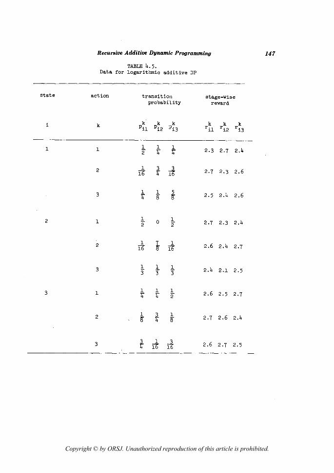
EXAMPLE 5 (Logarithmic Additive DP)

k k This is the case where f'ij == log r ij' t (r) = r in the

recursive additive DP {S, A, p, r, (3, t}. Then, the logarithmic

addi ti ve RS ,is given as follows

(log rl·log r 2··· log rn_l)rn+ •••.

( ) 1 <. k In this DP Assumption I means that - r ij <: e for i EO S,

k~ Ai' j~S. The following data satisfies Assumption (I).



TABLE 4.5. Data for logarithmic additive DP

state action transition stage-wise probability reward

i k k k k k k k pU Pi2 Pi3 rn r i2 ri3

1 1 1 1 1 2.3 2.7 2.4 2 4" 4"

2 1 3 3 2.7 2.3 2.6 lb 4" Ib

3 1 1 i 2.5 2.4 2.6 4" 8"

2 1 1 0

1 2.7 2.3 2.4 2 2

2 1 7 1 2.6 2.4 2.7 lb 8 ib

3 1 1 1 2.4 2.1 2.5 3 3" 3"

3 1 1 1 1 2.6 2.5 2.7 4" 4" 2"

2 1 3 1 2.7 2.6 2.4 8" 4" 8"

3 3 1 3 2.6 2.7 2.5 4" lb j:b


148 Seiichi /wamoto

Then optimal S-policy is f~) and optimal return is

(00) (52.3188) V(f ) = 52.0526, where

53.7307 f = cV .

The LP problem (PT) with an initial distribution

tX = 1 ( 2'

11 12312 4' 4) gives an optimal solution (Yl' Yl' Yl ' Y2 ' Y2'

3 1 Y2' Y3' y~, Y§) = (0.0,0.0,6.1654,3.3892,0.0,0.0,10.7585,0.0,0.0)

and an optimal value 52.6052.

Note that this value is

1 ( 52.3188) (2' ~,~) 52.0526

53.7307

We remark that above five examples are the case t(r)=r

in the recursive additive DP { S, A, p, r, f5' t} . But we can

1 r treat, for example, the case where t(r)=r' t(r)=e ,

t(r)=(l-r)er , t(r)=log r, etc., ([7]).

5. Further remarks

In this section we shall give some remarks on the recursive

additive DP.

Let {s, A, p, r, j3, t] be the recursive additive DP

satisfying Assumption (r). We define DP {s, A, p, r r in which

S v{o} , o (t\ S) is a ficti tious state I



1 1 i=O, k=l, j=O,

i~S!, kEAi , j=O,

and i=O,k=l,j=O,

i, Y =k)=pk for i~S, kEAi

, jES, n ij

where P is a probability law associated with DP{ S, X, p, r] , and Xn , Yn (n21) denote observed state and action at n-th stage.

In other words, nonnagative p..~(n) satisfying (1) is the

joint probability of being in state i E: S and making decision

kEAi at the n-th stage regarding to above probability law P.

Furthermore above { S, X, p, r} gi ves DP with an absorved

state { o}. We can also apply the LP method for DP{S, X, p,

r} as well as DP{S, A, p, r'fJ' t} with Assumption (I).

But it is rather difficut to get five examples in section 4

from the reduced DP {s, X, p, r} .


l50 Seiichi /wamoto

Acknowledgement

The author wishes to express his hearty thanks to

Prof. N. Furukawa for his advices. He also thanks the referee

for his various comments and suggestions for improving this

paper.

References

[lJ Aris, R, Discrete Dynamic Programming, Blaisdell,

Publishing Company, New York Tront London, (1964).

[2J Bellman, R~ Dynamic Programming, Princeton Univ. Press,

Princeton, New Jersey, (1957).

[3J DeGhellinck, G.T. and Eppen, G.D., "Linear programming

solutions for separable Markovian decision problems",

Mangt. Sc1.,13, 371-394, (967).

[4J D'Epenoux, F.. "A probabilistic production and inventory

problem", Mangt. ScL, la. 98-108 (1963).

[5J Furukawa, N. and Iwamoto, s.. "Markovian decision processes

with recursive reward functions". Bull. Math. Statist.,

15. 3-4. 79-91. (1973).

[6J Howard. R.~. Dynamic Programming and Markov Processes,

M.I.T. Press, Cambridge, Massachusetts, (1960).

[7J Iwamoto, S., "Discrete dynamic programming with recursive

additive slst~~". Bull. Math. Statist., 16. 1-2,

49-66, (1974).

[8J Manne, A.S., "Linear programming and sequential decisions",

Mangt. Sc1., 6, 259-267, (960).



[9J Nemhauser, G.L~ Introduction to Dynamic Programming,

John Wiley and Sons, NewwYork London Sydney, (1966).

[lOJ Osaki, S. and Mine, Ho, "Linear programming algorithm

for semi-Markovian decision processes '; J. Math.

Anal. Appl., 22, 356-381, (1968).

[llJ Osaki, S.and Mine, H., "Some remarks on a Markovian

decision problem with an absorbing state", J.

Math. Anal. Appl., 23, 327-333, (1968).

151


Documents

LINEAR PROGRAMMING ON RECURSIVE ADDITIVE ...archive/pdf/e_mag/Vol.18_03_04_125.pdfJ. Operations Research Soc. of Japan Vol. 18, No. 3 & No. 4, September 1975 LINEAR PROGRAMMING ON