Linear Programming: Interior-Point Methodspages.cs.wisc.edu/~swright/726/handouts/ip_h.pdf · Chapter 14 Linear Programming: Interior-Point Methods In the 1980s it was discovered

Chapter 14

Linear Programming:Interior-Point Methods

In the 1980s it was discovered that many large linear programs could be solvedefficiently by formulating them as nonlinear problems and solving them withvarious modifications of nonlinear algorithms such as Newton’s method. Onecharacteristic of these methods was that they required all iterates to satisfythe inequality constraints in the problem strictly, so they became known asinterior-point methods. By the early 1990s, one class—primal-dual methods—had distinguished itself as the most efficient practical approach, and provedto be a strong competitor to the simplex method on large problems. Thesemethods are the focus of this chapter.

Interior-point methods arose from the search for algorithms with better the-oretical properties than the simplex method. As we mentioned in Chapter ??,the simplex method can be inefficient on certain pathological problems. Roughlyspeaking, the time required to solve a linear program may be exponential in thesize of the problem, as measured by the number of unknowns and the amountof storage needed for the problem data. For almost all practical problems,the simplex method is much more efficient than this bound would suggest, butits poor worst-case complexity motivated the development of new algorithmswith better guaranteed performance. The first such method was the ellipsoidmethod, proposed by Khachiyan [11], which finds a solution in time that is atworst polynomial in the problem size. Unfortunately, this method approachesits worst-case bound on all problems and is not competitive with the simplexmethod in practice.

Karmarkar’s projective algorithm [10], announced in 1984, also has the poly-nomial complexity property , but it came with the added inducement of goodpractical behavior. The initial claims of excellent performance on large linearprograms were never fully borne out, but the announcement prompted a greatdeal of research activity and a wide array of methods described by such labels as“affine-scaling,” “logarithmic barrier,” “potential-reduction,” “path-following,”

1

2 CHAPTER 14. INTERIOR-POINT METHODS

“primal-dual,” and “infeasible interior-point.” All are related to Karmarkar’soriginal algorithm, and to the log-barrier approach described in Chapter ??,but many of the approaches can be motivated and analyzed independently ofthe earlier methods.

Interior-point methods share common features that distinguish them fromthe simplex method. Each interior-point iteration is expensive to compute andcan make significant progress towards the solution, while the simplex methodusually requires a larger number of inexpensive iterations. Geometrically speak-ing, the simplex method works its way around the boundary of the feasiblepolytope, testing a sequence of vertices in turn until it finds the optimal one.Interior-point methods approach the boundary of the feasible set only in thelimit. They may approach the solution either from the interior or the exteriorof the feasible region, but they never actually lie on the boundary of this region.

In this chapter, we outline some of the basic ideas behind primal-dual interior-point methods, including the relationship to Newton’s method and homotopymethods and the concept of the central path. We sketch the important methodsin this class, and give a comprehensive convergence analysis of a long-step path-following method. We describe in some detail a practical predictor-correctoralgorithm proposed by Mehrotra, which is the basis of much of the currentgeneration of software.

14.1 Primal-Dual Methods

Outline

We consider the linear programming problem in standard form; that is,

min cT x, subject to Ax = b, x ≥ 0, (14.1)

where c and x are vectors in IRn, b is a vector in IRm, and A is an m×n matrix.The dual problem for (14.1) is

max bT λ, subject to AT λ + s = c, s ≥ 0, (14.2)

where λ is a vector in IRm and s is a vector in IRn. As shown in Chapter ??, so-lutions of (14.1),(14.2) are characterized by the Karush-Kuhn-Tucker conditions(??), which we restate here as follows:

AT λ + s = c, (14.3a)Ax = b, (14.3b)

xisi = 0, i = 1, 2, . . . , n, (14.3c)(x, s) ≥ 0. (14.3d)

Primal-dual methods find solutions (x∗, λ∗, s∗) of this system by applying vari-ants of Newton’s method to the three equalities in (14.3) and modifying the

14.1. PRIMAL-DUAL METHODS 3

search directions and step lengths so that the inequalities (x, s) ≥ 0 are satisfiedstrictly at every iteration. The equations (14.3a),(14.3b),(14.3c) are only mildlynonlinear and so are not difficult to solve by themselves. However, the prob-lem becomes much more difficult when we add the nonnegativity requirement(14.3d). This nonnegativity condition is the source of all the complications inthe design and analysis of interior-point methods.

To derive primal-dual interior-point methods we restate the optimality con-ditions (14.3) in a slightly different form by means of a mapping F from IR2n+m

to IR2n+m:

F (x, λ, s) =

AT λ + s − c

Ax − bXSe

= 0, (14.4a)

(x, s) ≥ 0, (14.4b)

whereX = diag(x1, x2, . . . , xn), S = diag(s1, s2, . . . , sn), (14.5)

and e = (1, 1, . . . , 1)T . Primal-dual methods generate iterates (xk, λk, sk) thatsatisfy the bounds (14.4b) strictly, that is, xk > 0 and sk > 0. This property isthe origin of the term interior-point. By respecting these bounds, the methodsavoid spurious solutions, that is, points that satisfy F (x, λ, s) = 0 but not(x, s) ≥ 0. Spurious solutions abound, and do not provide useful informationabout solutions of (14.1) or (14.2), so it makes sense to exclude them altogetherfrom the region of search.

Many interior-point methods actually require the iterates to be strictly fea-sible; that is, each (xk, λk, sk) must satisfy the linear equality constraints forthe primal and dual problems. If we define the primal-dual feasible set F andstrictly feasible set Fo by

F = (x, λ, s) |Ax = b, AT λ + s = c, (x, s) ≥ 0, (14.6a)Fo = (x, λ, s) |Ax = b, AT λ + s = c, (x, s) > 0, (14.6b)

the strict feasibility condition can be written concisely as

(xk, λk, sk) ∈ Fo.

Like most iterative algorithms in optimization, primal-dual interior-pointmethods have two basic ingredients: a procedure for determining the step and ameasure of the desirability of each point in the search space. The procedure fordetermining the search direction procedure has its origins in Newton’s methodfor the nonlinear equations (14.4a). Newton’s method forms a linear model forF around the current point and obtains the search direction (∆x, ∆λ, ∆s) bysolving the following system of linear equations:

J(x, λ, s)

∆x

∆s∆λ

= −F (x, λ, s),


where J is the Jacobian of F . (See Chapter ?? for a detailed discussion ofNewton’s method for nonlinear systems.) If the current point is strictly feasible(that is, (x, λ, s) ∈ Fo), the Newton step equations become

0 AT IA 0 0S 0 X

∆x

∆λ∆s

=

0

0−XSe

. (14.7)

Usually, a full step along this direction would violate the bound (x, s) ≥ 0. Toavoid this difficulty, we perform a line search along the Newton direction so thatthe new iterate is

(x, λ, s) + α(∆x, ∆λ, ∆s),

for some line search parameter α ∈ (0, 1]. Unfortunately, we often can takeonly a small step along this direction (α 1) before violating the condition(x, s) > 0. Hence, the pure Newton direction (14.7), which is known as theaffine scaling direction, often does not allow us to make much progress towarda solution.

Most primal-dual methods modify the basic Newton procedure in two im-portant ways:

1. They bias the search direction toward the interior of the nonnegative or-thant (x, s) ≥ 0, so that we can move further along the direction beforeone of the components of (x, s) becomes negative.

2. They prevent the components of (x, s) from moving “too close” to theboundary of the nonnegative orthant.

To describe these modifications, we need to introduce the concept of the centralpath, and of neighborhoods of this path.

The Central Path

The central path C is an arc of strictly feasible points that plays a vital rolein primal-dual algorithms. It is parametrized by a scalar τ > 0, and each point(xτ , λτ , sτ ) ∈ C solves the following system:

AT λ + s = c, (14.8a)Ax = b, (14.8b)

xisi = τ, i = 1, 2, . . . , n, (14.8c)(x, s) > 0. (14.8d)

These conditions differ from the KKT conditions only in the term τ on theright-hand side of (14.8c). Instead of the complementarity condition (14.3c), werequire that the pairwise products xisi have the same (positive) value for allindices i. From (14.8), we can define the central path as

C = (xτ , λτ , sτ ) | τ > 0.


It can be shown that (xτ , λτ , sτ ) is defined uniquely for each τ > 0 if and onlyif Fo is nonempty.

Another way of defining C is to use the mapping F defined in (14.4) andwrite

F (xτ , λτ , sτ ) =

0

0τe

, (xτ , sτ ) > 0. (14.9)

The equations (14.8) approximate (14.3) more and more closely as τ goesto zero. If C converges to anything as τ ↓ 0, it must converge to a primal-dualsolution of the linear program. The central path thus guides us to a solutionalong a route that maintains positivity of the x and s components and decreasesthe pairwise products xisi, i = 1, 2, . . . , n to zero at the same rate.

Primal-dual algorithms take Newton steps toward points on C for whichτ > 0, rather than pure Newton steps for F . Since these steps are biasedtoward the interior of the nonnegative orthant defined by (x, s) ≥ 0, it usuallyis possible to take longer steps along them than along the pure Newton (affinescaling) steps, before violating the positivity condition.

To describe the biased search direction, we introduce a centering parameterσ ∈ [0, 1] and a duality measure µ defined by

µ =1n

n∑i=1

xisi =xT s

n, (14.10)

which measures the average value of the pairwise products xisi. By fixingτ = σµ and applying Newton’s method to the system (14.9), we obtain

0 AT IA 0 0S 0 X

∆x

∆λ∆s

=

0

0−XSe + σµe

. (14.11)

The step (∆x, ∆λ, ∆s) is a Newton step toward the point (xσµ, λσµ, sσµ) ∈ C, atwhich the pairwise products xisi are all equal to σµ. In contrast, the step (14.7)aims directly for the point at which the KKT conditions (14.3) are satisfied.

If σ = 1, the equations (14.11) define a centering direction, a Newton steptoward the point (xµ, λµ, sµ) ∈ C, at which all the pairwise products xisi areidentical to the current average value of µ. Centering directions are usuallybiased strongly toward the interior of the nonnegative orthant and make little,if any, progress in reducing the duality measure µ. However, by moving closerto C, they set the scene for a substantial reduction in µ on the next iteration. Atthe other extreme, the value σ = 0 gives the standard Newton (affine scaling)step (14.7). Many algorithms use intermediate values of σ from the open interval(0, 1) to trade off between the twin goals of reducing µ and improving centrality.

A Primal-Dual Framework

With these basic concepts in hand, we can define a general framework forprimal-dual algorithms.


Framework 14.1 (Primal-Dual)Given (x0, λ0, s0) ∈ Fo

for k = 0, 1, 2, . . .Solve

0 AT I

A 0 0Sk 0 Xk

∆xk

∆λk

∆sk

=

0

0−XkSke + σkµke

, (14.12)

where σk ∈ [0, 1] and µk = (xk)T sk/n;Set

(xk+1, λk+1, sk+1) = (xk, λk, sk) + αk(∆xk, ∆λk, ∆sk), (14.13)

choosing αk so that (xk+1, sk+1) > 0.end (for).

The choices of centering parameter σk and step length αk are crucial tothe performance of the method. Techniques for controlling these parameters,directly and indirectly, give rise to a wide variety of methods with differenttheoretical properties.

So far, we have assumed that the starting point (x0, λ0, s0) is strictly feasibleand, in particular, that it satisfies the linear equations Ax0 = b, AT λ0 + s0 = c.All subsequent iterates also respect these constraints, because of the zero right-hand side terms in (14.12). For most problems, however, a strictly feasiblestarting point is difficult to find. Infeasible-interior-point methods require onlythat the components of x0 and s0 be strictly positive. The search directionneeds to be modified so that it improves feasibility as well as centrality at eachiteration, but this requirement entails only a slight change to the step equation(14.11). If we define the residuals for the two linear equations as

rb = Ax − b, rc = AT λ + s − c, (14.14)

the modified step equation is 0 AT I

A 0 0S 0 X

∆x

∆λ∆s

=

−rc

−rb

−XSe + σµe

. (14.15)

The search direction is still a Newton step toward the point (xσµ, λσµ, sσµ) ∈ C.It tries to correct all the infeasibility in the equality constraints in a single step.If a full step is taken at any iteration, (that is, αk = 1 for some k), the residualsrb and rc become zero, and all subsequent iterates remain strictly feasible.

We discuss infeasible-interior-point methods further in Section 14.3.

Central Path Neighborhoods and Path-Following Methods

Path-following algorithms explicitly restrict the iterates to a neighborhood ofthe central path C and follow C to a solution of the linear program. By preventing


C

central path neighborhood

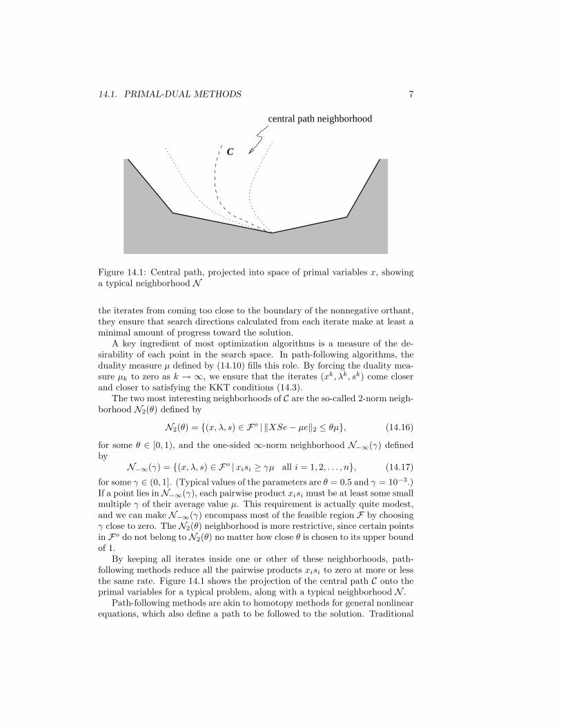
Figure 14.1: Central path, projected into space of primal variables x, showinga typical neighborhood N

the iterates from coming too close to the boundary of the nonnegative orthant,they ensure that search directions calculated from each iterate make at least aminimal amount of progress toward the solution.

A key ingredient of most optimization algorithms is a measure of the de-sirability of each point in the search space. In path-following algorithms, theduality measure µ defined by (14.10) fills this role. By forcing the duality mea-sure µk to zero as k → ∞, we ensure that the iterates (xk, λk, sk) come closerand closer to satisfying the KKT conditions (14.3).

The two most interesting neighborhoods of C are the so-called 2-norm neigh-borhood N2(θ) defined by

N2(θ) = (x, λ, s) ∈ Fo | ‖XSe − µe‖2 ≤ θµ, (14.16)

for some θ ∈ [0, 1), and the one-sided ∞-norm neighborhood N−∞(γ) definedby

N−∞(γ) = (x, λ, s) ∈ Fo |xisi ≥ γµ all i = 1, 2, . . . , n, (14.17)

for some γ ∈ (0, 1]. (Typical values of the parameters are θ = 0.5 and γ = 10−3.)If a point lies in N−∞(γ), each pairwise product xisi must be at least some smallmultiple γ of their average value µ. This requirement is actually quite modest,and we can make N−∞(γ) encompass most of the feasible region F by choosingγ close to zero. The N2(θ) neighborhood is more restrictive, since certain pointsin Fo do not belong to N2(θ) no matter how close θ is chosen to its upper boundof 1.

By keeping all iterates inside one or other of these neighborhoods, path-following methods reduce all the pairwise products xisi to zero at more or lessthe same rate. Figure 14.1 shows the projection of the central path C onto theprimal variables for a typical problem, along with a typical neighborhood N .

Path-following methods are akin to homotopy methods for general nonlinearequations, which also define a path to be followed to the solution. Traditional


homotopy methods stay in a tight tubular neighborhood of their path, makingincremental changes to the parameter and chasing the homotopy path all theway to a solution. For primal-dual methods, this neighborhood is conical ratherthan tubular, and it tends to be broad and loose for larger values of the dualitymeasure µ. It narrows as µ → 0, however, because of the positivity requirement(x, s) > 0.

The algorithm we specify below, a special case of Framework 14.1, is knownas a long-step path-following algorithm. This algorithm can make rapid progressbecause of its use of the wide neighborhood N−∞(γ), for γ close to zero. Itdepends on two parameters σmin and σmax, which are upper and lower boundson the centering parameter σk. The search direction is, as usual, obtained bysolving (14.12), and we choose the step length αk to be as large as possible,subject to the requirement that we stay inside N−∞(γ).

Here and in later analysis, we use the notation

(xk(α), λk(α), sk(α)) def= (xk, λk, sk) + α(∆xk , ∆λk, ∆sk), (14.18a)

µk(α) def= xk(α)T sk(α)/n. (14.18b)

Algorithm 14.2 (Long-Step Path-Following)Given γ, σmin, σmax with γ ∈ (0, 1), 0 < σmin < σmax < 1,

and (x0, λ0, s0) ∈ N−∞(γ);for k = 0, 1, 2, . . .

Choose σk ∈ [σmin, σmax];Solve (14.12) to obtain (∆xk, ∆λk, ∆sk);Choose αk as the largest value of α in [0, 1] such that

(xk(α), λk(α), sk(α)) ∈ N−∞(γ); (14.19)

Set (xk+1, λk+1, sk+1) = (xk(αk), λk(αk), sk(αk));end (for).

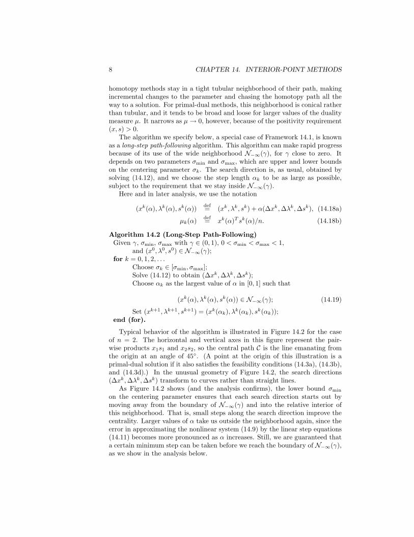
Typical behavior of the algorithm is illustrated in Figure 14.2 for the caseof n = 2. The horizontal and vertical axes in this figure represent the pair-wise products x1s1 and x2s2, so the central path C is the line emanating fromthe origin at an angle of 45. (A point at the origin of this illustration is aprimal-dual solution if it also satisfies the feasibility conditions (14.3a), (14.3b),and (14.3d).) In the unusual geometry of Figure 14.2, the search directions(∆xk, ∆λk, ∆sk) transform to curves rather than straight lines.

As Figure 14.2 shows (and the analysis confirms), the lower bound σmin

on the centering parameter ensures that each search direction starts out bymoving away from the boundary of N−∞(γ) and into the relative interior ofthis neighborhood. That is, small steps along the search direction improve thecentrality. Larger values of α take us outside the neighborhood again, since theerror in approximating the nonlinear system (14.9) by the linear step equations(14.11) becomes more pronounced as α increases. Still, we are guaranteed thata certain minimum step can be taken before we reach the boundary of N−∞(γ),as we show in the analysis below.

14.2. ANALYSIS OF ALGORITHM 14.2 9

x2 s2

x1 s1

iterates 01

2

3

central path C

Nboundary of neighborhood

Figure 14.2: Iterates of Algorithm 14.2, plotted in (xs) space

We present a complete analysis of Algorithm 14.2, which makes use of sur-prisingly simple mathematical foundations, in Section 14.2 below. With judi-cious choices of σk, this algorithm is fairly efficient in practice. With a few morechanges it becomes the basis of a truly competitive method, as we discuss inSection 14.3.

An infeasible-interior-point variant of Algorithm 14.2 can be constructed bygeneralizing the definition of N−∞(γ) to allow violation of the feasibility con-ditions. In this extended neighborhood, the residual norms ‖rb‖ and ‖rc‖ arebounded by a constant multiple of the duality measure µ. By squeezing µ tozero, we also force rb and rc to zero, so that the iterates approach complemen-tarity and feasibility at the same time.

14.2 Analysis of Algorithm 14.2

We now present a comprehensive analysis of Algorithm 14.2. Our aim is to showthat given some small tolerance ε > 0, and given some mild assumptions aboutthe starting point (x0, λ0, s0), the algorithm requires O(n| log ε|) iterations toidentify a point (xk, λk, sk) for which µk ≤ ε, where µk = (xk)T sk/n. For smallε, the point (xk, λk, sk) satisfies the primal-dual optimality conditions except forperturbations of about ε in the right-hand side of (14.3c), so it is usually veryclose to a primal-dual solution of the original linear program. The O(n| log ε|)estimate is a worst-case bound on the number of iterations required; on practicalproblems, the number of iterations required appears to increase only slightly as


n increases. The simplex method may require 2n iterations to solve a problemwith n variables, though in practice it usually requires a modest multiple ofmax(m, n) iterations, where m is the row dimension of the constraint matrix Ain (14.1).

As is typical for interior-point methods, the analysis builds from a purelytechnical lemma to a powerful theorem in just a few pages. We start with thetechnical lemma—Lemma 14.1—and use it to prove Lemma 14.2, a bound onthe vector of pairwise products ∆xi∆si, i = 1, 2, . . . , n. Theorem 14.3 finds alower bound on the step length αk and a corresponding estimate of the reductionin µ on iteration k. Finally, Theorem 14.4 proves that O(n| log ε|) iterations arerequired to identify a point for which µk < ε, for a given tolerance ε ∈ (0, 1).

Lemma 14.1 Let u and v be any two vectors in IRn with uT v ≥ 0. Then

‖UV e‖ ≤ 2−3/2‖u + v‖2,

whereU = diag(u1, u2, . . . , un), V = diag(v1, v2, . . . , vn).

Proof. First, note that for any two scalars α and β with αβ ≥ 0, we havefrom the algebraic-geometric mean inequality that√

|αβ| ≤ 12|α + β|. (14.20)

Since uT v ≥ 0, we have

0 ≤ uT v =∑

uivi≥0

uivi +∑

uivi<0

uivi =∑i∈P

|uivi| −∑i∈M

|uivi|, (14.21)

where we partitioned the index set 1, 2, . . . , n as

P = i |uivi ≥ 0, M = i |uivi < 0.Now,

‖UV e‖ =(‖[uivi]i∈P‖2 + ‖[uivi]i∈M‖2

)1/2

≤(‖[uivi]i∈P‖2

1 + ‖[uivi]i∈M‖21

)1/2

since ‖ · ‖2 ≤ ‖ · ‖1

≤(2 ‖[uivi]i∈P‖2

1

)1/2

from (14.21)

≤√

2∥∥∥∥[14(ui + vi)2

]i∈P

∥∥∥∥1

from (14.20)

= 2−3/2∑i∈P

(ui + vi)2

≤ 2−3/2n∑

i=1

(ui + vi)2

≤ 2−3/2‖u + v‖2,


completing the proof.

Lemma 14.2 If (x, λ, s) ∈ N−∞(γ), then

‖∆X∆Se‖ ≤ 2−3/2(1 + 1/γ)nµ.

Proof. It is easy to show using (14.12) that

∆xT ∆s = 0. (14.22)

By multiplying the last block row in (14.12) by (XS)−1/2 and using the defini-tion D = X1/2S−1/2, we obtain

D−1∆x + D∆s = (XS)−1/2(−XSe + σµe). (14.23)

Because (D−1∆x)T (D∆s) = ∆xT ∆s = 0, we can apply Lemma 14.1 withu = D−1∆x and v = D∆s to obtain

‖∆X∆Se‖ = ‖(D−1∆X)(D∆S)e‖≤ 2−3/2‖D−1∆x + D∆s‖2 from Lemma 14.1

= 2−3/2‖(XS)−1/2(−XSe + σµe)‖2 from (14.23).

Expanding the squared Euclidean norm and using such relationships as xT s =nµ and eT e = n, we obtain

‖∆X∆Se‖ ≤ 2−3/2

[xT s − 2σµeT e + σ2µ2

n∑i=1

1xisi

]

≤ 2−3/2

[xT s − 2σµeT e + σ2µ2 n

γµ

]since xisi ≥ γµ

≤ 2−3/2

[1 − 2σ +

σ2

γ

]nµ

≤ 2−3/2(1 + 1/γ)nµ,

as claimed.

Theorem 14.3 Given the parameters γ, σmin, and σmax in Algorithm 14.2,there is a constant δ independent of n such that

µk+1 ≤(

1 − δ

n

)µk, (14.24)

for all k ≥ 0.

Proof. We start by proving that

(xk(α), λk(α), sk(α)

) ∈ N−∞(γ) for all α ∈[0, 23/2γ

1 − γ

1 + γ

σk

n

], (14.25)


where(xk(α), λk(α), sk(α)

)is defined as in (14.18). It follows that the step

length αk is at least as long as the upper bound of this interval, that is,

αk ≥ 23/2 σk

nγ

1 − γ

1 + γ. (14.26)

For any i = 1, 2, . . . , n, we have from Lemma 14.2 that

|∆xki ∆sk

i | ≤ ‖∆Xk∆Ske‖2 ≤ 2−3/2(1 + 1/γ)nµk. (14.27)

Using (14.12), we have from xki sk

i ≥ γµk and (14.27) that

xki (α)sk

i (α) =(xk

i + α∆xki

) (sk

i + α∆ski

)= xk

i ski + α

(xk

i ∆ski + sk

i ∆xki

)+ α2∆xk

i ∆ski

≥ xki sk

i (1 − α) + ασkµk − α2|∆xki ∆sk

i |≥ γ(1 − α)µk + ασkµk − α22−3/2(1 + 1/γ)nµk.

By summing the n components of the equation Sk∆xk + Xk∆sk = −XkSke +σkµke (the third block row from (14.12)), and using (14.22) and the definitionof µk and µk(α) (see (14.18)), we obtain

µk(α) = (1 − α(1 − σk))µk.

From these last two formulas, we can see that the proximity condition

xki (α)sk

i (α) ≥ γµk(α)

is satisfied, provided that

γ(1 − α)µk + ασkµk − α22−3/2(1 + 1/γ)nµk ≥ γ(1 − α + ασk)µk.

Rearranging this expression, we obtain

ασkµk(1 − γ) ≥ α22−3/2nµk(1 + 1/γ),

which is true if

α ≤ 23/2

nσkγ

1 − γ

1 + γ.

We have proved that(xk(α), λk(α), sk(α)

)satisfies the proximity condition for

N−∞(γ) when α lies in the range stated in (14.25). It is not difficult to showthat

(xk(α), λk(α), sk(α)

) ∈ Fo for all α in the given range (see the exercises).Hence, we have proved (14.25) and therefore (14.26).

We complete the proof of the theorem by estimating the reduction in µ onthe kth step. Because of (14.22), (14.26), and the last block row of (14.11), wehave

µk+1 = xk(αk)T sk(αk)/n

=[(xk)T sk + αk

((xk)T ∆sk + (sk)T ∆xk

)+ α2

k(∆xk)T ∆sk]/n(14.28)

= µk + αk

(−(xk)T sk/n + σkµk

)(14.29)

= (1 − αk(1 − σk))µk (14.30)

≤(

1 − 23/2

nγ

1 − γ

1 + γσk(1 − σk)

)µk. (14.31)


Now, the function σ(1−σ) is a concave quadratic function of σ, so on any giveninterval it attains its minimum value at one of the endpoints. Hence, we have

σk(1 − σk) ≥ min σmin(1 − σmin), σmax(1 − σmax) , for all σk ∈ [σmin, σmax].

The proof is completed by substituting this estimate into (14.31) and setting

δ = 23/2γ1 − γ

1 + γmin σmin(1 − σmin), σmax(1 − σmax) .

We conclude with the complexity result.

Theorem 14.4 Given ε > 0 and γ ∈ (0, 1), suppose the starting point (x0, λ0, s0) ∈N−∞(γ) in Algorithm 14.2 has

µ0 ≤ 1/εκ (14.32)

for some positive constant κ. Then there is an index K with K = O(n log 1/ε)such that

µk ≤ ε, for all k ≥ K.

Proof. By taking logarithms of both sides in (14.24), we obtain

log µk+1 ≤ log(

1 − δ

n

)+ log µk.

By repeatedly applying this formula and using (14.32), we have

log µk ≤ k log(

1 − δ

n

)+ log µ0 ≤ k log

(1 − δ

n

)+ κ log

1ε.

The following well-known estimate for the log function,

log(1 + β) ≤ β, for all β > −1,

implies that

log µk ≤ k

(− δ

n

)+ κ log

1ε.

Therefore, the convergence criterion µk ≤ ε is satisfied if we have

k

(− δ

n

)+ κ log

1ε≤ log ε.

This inequality holds for all k that satisfy

k ≥ K = (1 + κ)n

δlog

1ε,

so the proof is complete.


14.3 Practical Primal-Dual Algorithms

Practical implementations of interior-point algorithms follow the spirit of thetheory in the previous section, in that strict positivity of xk and sk is main-tained throughout and each step is a Newton-like step involving a centeringcomponent. However, several aspects of “theoretical” algorithms are typicallyignored, while several enhancements are added that have a significant effect onpractical performance. We discuss in this section the algorithmic enhancementsthat are present in most interior-point software.

Practical implementations typically do not enforce membership of the centralpath neighborhoods N2 and N−∞ defined in the previous section. Rather, theycalculate the maximum steplengths that can be taken in the x and s variables(separately) without violating nonnegativity, then take a steplength of slightlyless than this maximum. Given an iterate (xk, λk, sk) with (xk, sk) > 0, and astep (∆xk, ∆λk, ∆sk), it is easy to show that the quantities αpri

k,max and αdualk,max

defined as follows:

αprik,max

def= mini:∆xk

i <0− xk

i

∆xki

, (14.33a)

αdualk,max

def= mini:∆sk

i <0− sk

i

∆ski

, (14.33b)

are the largest values of α for which xk + α∆xk ≥ 0 and sk + α∆sk ≥ 0,respectively. Practical algorithms then choose the steplengths to lie in the openintervals defined by these maxima, that is,

αprik ∈ (0, αpri

k,max), αdualk ∈ (0, αdual

k,max),

and then obtain a new iterate by setting

xk+1 = xk + αprik ∆xk, (λk+1, sk+1) = (λk, sk) + αdual

k (∆λk, ∆sk).

If the step (∆xk, ∆λk, ∆sk) rectifies the infeasibility in the KKT conditions(14.3a) and (14.3b), that is,

A∆xk = −rkb = −(Axk − b), AT ∆λk + ∆sk = −rk

c = −(AT λk + sk − c),

it is easy to show that the infeasibilities at the new iterate satisfy

rk+1b =

(1 − αpri

k

)rkb , rk+1

c =(1 − αdual

k

)rkc , (14.34)

where rk+1b and rk+1

c are defined in the obvious way.A second feature of practical algorithms is their use of corrector steps, a

development made practical by Mehrotra [14]. These steps compensate for thelinearization error made by the Newton (affine-scaling) step in modeling theequation xisi = 0, i = 1, 2, . . . , n (see (14.3c)). Consider the affine-scaling

14.3. PRACTICAL PRIMAL-DUAL ALGORITHMS 15

direction (∆x, ∆λ, ∆s) defined by

0 AT I

A 0 0S 0 X

∆xaff

∆λaff

∆saff

=

−rc

−rb

−XSe

, (14.35)

(where rb and rc are defined in (14.14)). If we take a full step in this direction,we obtain

(xi + ∆xaffi )(si + ∆saff

i )= xisi + xi∆saff

i + si∆xaffi + ∆xaff

i ∆saffi = ∆xaff

i ∆saffi .

That is, the updated value of xisi is ∆xaffi ∆saff

i rather than the ideal value 0.We can solve the following system to obtain a step (∆xcor, ∆λcor, ∆scor) thatcorrects for this deviation from the ideal:

0 AT IA 0 0S 0 X

∆xcor

∆λcor

∆scor

=

0

0−∆Xaff∆Saffe

. (14.36)

In many cases, the combined step (∆xaff , ∆λaff , ∆saff) + (∆xcor, ∆λcor, ∆scor)does a better job of reducing the duality measure than does the affine-scalingstep alone.

Like theoretical algorithms such as the one analysed in Section ??, practicalalgorithms make use of centering steps, with an adaptive choice of the centeringparameter σk. Mehrotra [14] introduced a highly successful scheme for choosingσk based on the effectiveness of the affine-scaling step at iteration k. Roughly,if the affine-scaling step (multiplied by a steplength to maintain nonnegativityof x and s) reduces the duality measure significantly, there is not much needfor centering, so a smaller value of σk is appropriate. Conversely, if not muchprogress can be made along this direction before reaching the boundary of thenonnegative orthant, a larger value of σk will ensure that the next iterate ismore centered, so a longer step will be possible from this next point. Specif-ically, Mehrotra’s scheme calculates the maximum allowable steplengths alongthe affine-scaling direction (14.35) as follows:

αpriaff

def= min

(1, min

i:∆xaffi <0

− xi

∆xaffi

), (14.37a)

αdualaff

def= min

(1, min

i:∆saffi <0

− si

∆saffi

), (14.37b)

and then defines µaff to be the value of µ that would be obtained by using thesesteplengths, that is,

µaff = (x + αpriaff ∆xaff)T (s + αdual

aff ∆saff)/n. (14.38)


The centering parameter σ is then chosen as follows:

σ =(

µaff

µ

)3

. (14.39)

To summarize, computation of the search direction in Mehrotra’s methodrequires the solution of two linear systems. First, the system (14.35) is solvedto obtain the affine-scaling direction, also known as the predictor step. Thisstep is used to define the right-hand side for the corrector step (see (14.36)) andto calculate the centering parameter from (14.38), (14.39). Second, the searchdirection is calculated by solving

0 AT IA 0 0S 0 X

∆x

∆λ∆s

=

−rc

−rb

−XSe − ∆Xaff∆Saffe + σµe

. (14.40)

Note that the predictor, corrector, and centering contributions have been ag-gregated on the right-hand side of this system. The coefficient matrix in bothlinear systems (14.35) and (14.40) is the same. Thus, the factorization of thematrix needs to be computed only once, and the marginal cost of solving thesecond system is relatively small.

Once the search direction has been calculated, the maximum steplengthsalong this direction are computed from (14.33), and the steplengths actuallyused are chosen to be

αprik = min(1, ηkαpri

max), αdualk = min(1, ηkαdual

max), (14.41)

where ηk ∈ [0.9, 1.0) is chosen so that ηk → 1 as the iterates approach theprimal-dual solution, solution, to accelerate the asymptotic convergence. (Fordetails on how η is chosen and on other elements of the algorithm such as thechoice of starting point (x0, λ0, s0), see Mehrotra [14].)

We now specify the algorithm in the usual format.

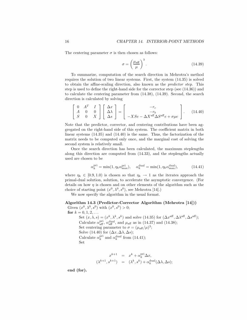
Algorithm 14.3 (Predictor-Corrector Algorithm (Mehrotra [14]))Given (x0, λ0, s0) with (x0, s0) > 0;for k = 0, 1, 2, . . .

Set (x, λ, s) = (xk, λk, sk) and solve (14.35) for (∆xaff , ∆λaff , ∆saff);Calculate αpri

aff , αdualaff , and µaff as in (14.37) and (14.38);

Set centering parameter to σ = (µaff/µ)3;Solve (14.40) for (∆x, ∆λ, ∆s);Calculate αpri

k and αdualk from (14.41);

Set

xk+1 = xk + αprik ∆x,

(λk+1, sk+1) = (λk, sk) + αdualk (∆λ, ∆s);

end (for).

14.3. PRACTICAL PRIMAL-DUAL ALGORITHMS 17

No convergence theory is available for Mehrotra’s algorithm, at least in theform in which it is described above. In fact, there are examples for which thealgorithm diverges. Simple safeguards could be incorporated into the methodto force it into the convergence framework of existing methods. However, mostprograms do not implement these safeguards, because the good practical per-formance of Mehrotra’s algorithm makes them unnecessary.

When presented with a linear program that is infeasible or unbounded, thealgorithm above typically diverges, with the infeasibilities rk

b and rkc and/or the

duality measure µk going to ∞. Since the symptoms of infeasibility and un-boundedness are fairly easy to recognize, interior-point codes contain heuristicsto detect and report these conditions. More rigorous approaches for detectinginfeasibility and unboundedness make use of the homogeneous self-dual formu-lation; see Wright [24, Chapter 9] and the references therein for a discussion. Amore recent approach that applies directly to infeasible-interior-point methodsis described by Todd [20]

Solving the Linear Systems

Most of the computational effort in primal-dual methods is taken up insolving linear systems such as (14.15), (14.35), and (14.40). The coefficientmatrix in these systems is usually large and sparse, since the constraint matrixA is itself large and sparse in most applications. The special structure in thestep equations allows us to reformulate them as systems with more compactsymmetric coefficient matrices, which are easier and cheaper to factor than theoriginal sparse form.

We apply the reformulation procedures to the following general form of thelinear system:

0 AT IA 0 0S 0 X

∆x

∆λ∆s

=

−rc

−rb

−rxs

. (14.42)

Since x and s are strictly positive, the diagonal matrices X and S are nonsingu-lar. Hence, by eliminating ∆s from (14.42), we obtain the following equivalentsystem:

[0 A

AT −D−2

] [∆λ∆x

]=

[ −rb

−rc + X−1rxs

], (14.43a)

∆s = −X−1rxs − X−1S∆x, (14.43b)

where we have introduced the notation

D = S−1/2X1/2. (14.44)

This form of the step equations usually is known as the augmented system. Sincethe matrix X−1S is also diagonal and nonsingular, we can go a step further,


eliminating ∆x from (14.43a) to obtain another equivalent form:

AD2AT ∆λ = −rb − AXS−1rc + AS−1rxs (14.45a)∆s = −rc − AT ∆λ, (14.45b)∆x = −S−1rxs − XS−1∆s. (14.45c)

This form often is called the normal-equations form because the system (14.45a)can be viewed as the normal equations (??) for a linear least-squares problemwith coefficient matrix DAT .

Most implementations of primal-dual methods are based on formulationslike (14.45). They use direct sparse Cholesky algorithms to factor the matrixAD2AT , and then perform triangular solves with the resulting sparse factorsto obtain the step ∆λ from (14.45a). The steps ∆s and ∆x are recoveredfrom (14.45b) and (14.45c). General-purpose sparse Cholesky software can beapplied to AD2AT , but a few modifications are needed because AD2AT maybe ill-conditioned or singular. (Ill conditioning of this system is often observedduring the final stages of a primal-dual algorithm, when the elements of thediagonal weighting matrix D2 take on both huge and tiny values.)

A disadvantage of this formulation is that if A contains any dense columns,the matrix AD2AT is completely dense. Hence, practical software identifiesdense and nearly-dense columns, excludes them from the matrix product AD2AT ,and performs the Cholesky factorization of the resulting sparse matrix. Then,a device such as a Sherman-Morrison-Woodbury update is applied to accountfor the excluded columns. We refer the reader to Wright [24, Chapter 11] forfurther details.

The formulation (14.43) has received less attention than (14.45), mainlybecause algorithms and software for factoring sparse symmetric indefinite ma-trices are more complicated, slower, and less prevalent than sparse Choleskyalgorithms. Nevertheless, the formulation (14.43) is cleaner and more flexiblethan (14.45) in a number of respects. We avoid the fill-in caused by densecolumns in A in the matrix product AD2AT , and free variables (that is, com-ponents of x with no explicit lower or upper bounds) can be handled withoutresorting to the various artificial devices needed in the normal-equations form.

14.4 Other Primal-Dual Algorithms and Exten-sions

Other Path-Following Methods

Framework 14.1 is the basis of a number of other algorithms of the path-following variety. They are less important from a practical viewpoint, but wemention them here because of their elegance and their strong theoretical prop-erties.

Some path-following methods choose conservative values for the centeringparameter σ (that is, σ only slightly less than 1) so that unit steps (that is,

14.4. OTHER PRIMAL-DUAL ALGORITHMS AND EXTENSIONS 19

a steplength of α = 1) can be taken along the resulting direction from (14.11)without leaving the chosen neighborhood. These methods, which are known asshort-step path-following methods, make only slow progress toward the solutionbecause they require the iterates to stay inside a restrictive N2 neighborhood(14.16).

Better results are obtained with the predictor-corrector method, due toMizuno, Todd, and Ye [15], which uses two N2 neighborhoods, nested one insidethe other. (Despite the similar terminology, this algorithm is quite distinct fromAlgorithm 14.3 of Section 14.3.) Every second step of this method is a predictorstep, which starts in the inner neighborhood and moves along the affine-scalingdirection (computed by setting σ = 0 in (14.11)) to the boundary of the outerneighborhood. The gap between neighborhood boundaries is wide enough toallow this step to make significant progress in reducing µ. Alternating with thepredictor steps are corrector steps (computed with σ = 1 and α = 1), whichtake the next iterate back inside the inner neighborhood in preparation for thenext predictor step. The predictor-corrector algorithm produces a sequence ofduality measures µk that converge superlinearly to zero, in contrast to the linearconvergence that characterizes most methods.

Potential-Reduction Methods

Potential-reduction methods take steps of the same form as path-followingmethods, but they do not explicitly follow the central path C and can be moti-vated independently of it. They use a logarithmic potential function to measurethe worth of each point in Fo and aim to achieve a certain fixed reduction inthis function at each iteration. The primal-dual potential function, which wedenote generically by Φ, usually has two important properties:

Φ → ∞ if xisi → 0 for some i, while µ = xT s/n → 0, (14.46a)Φ → −∞ if and only if (x, λ, s) → Ω. (14.46b)

The first property (14.46a) prevents any one of the pairwise products xisi fromapproaching zero independently of the others, and therefore keeps the iteratesaway from the boundary of the nonnegative orthant. The second property(14.46b) relates Φ to the solution set Ω. If our algorithm forces Φ to −∞, then(14.46b) ensures that the sequence approaches the solution set.

An interesting primal-dual potential function is the Tanabe-Todd-Ye func-tion Φρ defined by

Φρ(x, s) = ρ log xT s −n∑

i=1

log xisi, (14.47)

for some parameter ρ > n (see [17], [21]). Like all algorithms based on Frame-work 14.1, potential-reduction algorithms obtain their search directions by solv-ing (14.12), for some σk ∈ (0, 1), and they take steps of length αk along thesedirections. For instance, the step length αk may be chosen to approximatelyminimize Φρ along the computed direction. By fixing σk = n/(n+

√n) for all k,


one can guarantee constant reduction in Φρ at every iteration. Hence, Φρ willapproach −∞, forcing convergence. Adaptive and heuristic choices of σk and αk

are also covered by the theory, provided that they at least match the reductionin Φρ obtained from the conservative theoretical values of these parameters.

Extensions

Primal-dual methods for linear programming can be extended to wider classesof problems. There are simple extensions of the algorithm to the monotone lin-ear complementarity problem (LCP) and convex quadratic programming prob-lems for which the convergence and polynomial complexity properties of thelinear programming algorithms are retained. The LCP is the problem of findingvectors x and s in IRn that satisfy the following conditions:

s = Mx + q, (x, s) ≥ 0, xT s = 0, (14.48)

where M is a positive semidefinite n × n matrix and q ∈ IRn. The similar-ity between (14.48) and the KKT conditions (14.3) is obvious: The last twoconditions in (14.48) correspond to (14.3d) and (14.3c), respectively, while thecondition s = Mx + q is similar to the equations (14.3a) and (14.3b). Forpractical instances of the problem (14.48), see Cottle, Pang, and Stone [3].

In convex quadratic programming, we minimize a convex quadratic objectivesubject to linear constraints. A convex quadratic generalization of the standardform linear program (14.1) is

min cT x + 12xT Gx, subject to Ax = b, x ≥ 0, (14.49)

where G is a symmetric n × n positive semidefinite matrix. The KKT condi-tions for this problem are similar to those for linear programming (14.3) andalso to the linear complementarity problem (14.48). See Section ?? for furtherdiscussion of interior-point methods for (14.49).

Primal-dual methods for nonlinear programming problems can be devised bywriting down the KKT conditions in a form similar to (14.3), adding slack vari-ables where necessary to convert all the inequality conditions to simple boundsof the type (14.3d). As in Framework 14.1, the basic primal-dual step is found byapplying a modified Newton’s method to some formulation of these KKT condi-tions, curtailing the step length to ensure that the bounds are satisfied strictlyby all iterates. When the nonlinear programming problem is convex (that is,its objective and constraint functions are all convex functions), global conver-gence of primal-dual methods can be proved. Extensions to general nonlinearprogramming problems are not so straightforward; this topic is the subject ofChapter ??.

Interior-point methods are highly effective in solving semidefinite program-ming problems, a class of problems involving symmetric matrix variables thatare constrained to be positive semidefinite. Semidefinite programming, whichhas been the topic of concentrated research since the early 1990s, has applica-tions in many areas, including control theory and combinatorial optimization.

14.5. PERSPECTIVES AND SOFTWARE 21

Further information on this increasingly important topic can be found in thesurvey papers of Todd [19] and Vandenberghe and Boyd [22] and the books ofNesterov and Nemirovskii [16], Boyd et al. [1], and Boyd and Vandenberghe [2].

14.5 Perspectives and Software

The appearance of interior-point methods in the 1980s presented the first seri-ous challenge to the dominance of the simplex method as a practical means ofsolving linear programming problems. By about 1990, interior-point codes hademerged that incorporated the techniques described in Section 14.3 and thatwere superior on many large problems to the simplex codes available at thattime. The years that followed saw a quantum improvement in simplex software,evidenced by the appearance of packages such as CPLEX and XPRESS-MP.These improvements were due to algorthmic advances such as steepest-edgepivoting (See Goldfarb and Forrest [8]) and improved pricing heuristics, andalso to close attention to the nuts and bolts of efficient implementation. Theefficiency of interior-point codes also continued to improve, through improve-ments in the linear algebra for solving the step equations and through the useof higher-order correctors in the step calculation (see Gondzio [9]). During thisperiod, a number of good interior-point codes became freely available, at leastfor research use, and found their way into many applications.

In general, simplex codes are faster on problems of small-medium dimensions,while interior-point codes are competitive and often faster on large problems.However, this rule is certainly not hard-and-fast; it depends strongly on thestructure of the particular application. Interior-point methods are generallynot able to take advantage of prior knowledge about the solution, such as anestimate of the solution itself or an estimate of the optimal basis. Hence, thesemethods are less useful than simplex approaches in situations in which “warm-start” information is readily available. The most widespread situation of thistype involves branch-and-bound algorithms for solving integer programs, whereeach node in the branch-and-bound tree requires the solution of a linear programthat differs only slightly from one already solved in the parent node.

Interior-point software has the advantage that it is easy to program, relativeto the simplex method. The most complex operation is the solution of the largelinear systems at each iteration to compute the step; software to perform thislinear algebra operation is readily available. The interior-point code LIPSOL[25] is written entirely in the Matlab language, apart from a small amount ofFORTRAN code that interfaces to the linear algebra software. The code PCx[4] is written in C, but also is easy for the interested user to comprehend andmodify. It is even possible for a non-expert in optimization to write an efficientinterior-point implementation from scratch that is customized to their particularapplication.

Notes and References


For more details on the material of this chapter, see the book by Wright [24].As noted in the text, Karmarkar’s method arose from a search for linear pro-

gramming algorithms with better worst-case behavior than the simplex method.The first algorithm with polynomial complexity, Khachiyan’s ellipsoid algorithm[11], was a computational disappointment. In contrast, the execution times re-quired by Karmarkar’s method were not too much greater than simplex codes atthe time of its introduction, particularly for large linear programs. Karmarkar’sis a primal algorithm; that is, it is described, motivated, and implemented purelyin terms of the primal problem (14.1) without reference to the dual. At eachiteration, Karmarkar’s algorithm performs a projective transformation on theprimal feasible set that maps the current iterate xk to the center of the set andtakes a step in the feasible steepest descent direction for the transformed space.Progress toward optimality is measured by a logarithmic potential function.Nice descriptions of the algorithm can be found in Karmarkar’s original paper[10] and in Fletcher [7].

Karmarkar’s method falls outside the scope of this chapter, and in any case,its practical performance does not appear to match the most efficient primal-dual methods. The algorithms we discussed in this chapter have polynomialcomplexity, like Karmarkar’s method.

Many of the algorithmic ideas that have been examined since 1984 actuallyhad their genesis in three works that preceded Karmarkar’s paper. The first ofthese is the book of Fiacco and McCormick [6] on logarithmic barrier functions,which proves existence of the central path, among many other results. Furtheranalysis of the central path was carried out by McLinden [12], in the contextof nonlinear complementarity problems. Finally, there is Dikin’s paper [5], inwhich an interior-point method known as primal affine-scaling was originallyproposed. The outburst of research on primal-dual methods, which culminatedin the efficient software packages available today, dates to the seminal paper ofMegiddo [13].

Todd gives an excellent survey of potential reduction methods in [18]. Herelates the primal-dual potential reduction method mentioned above to pureprimal potential reduction methods, including Karmarkar’s original algorithm,and discusses extensions to special classes of nonlinear problems.

For an introduction to complexity theory and its relationship to optimiza-tion, see the book by Vavasis [23].

Exercises

1. This exercise illustrates the fact that the bounds (x, s) ≥ 0 are essential inrelating solutions of the system (14.4a) to solutions of the linear program(14.1) and its dual. Consider the following linear program in IR2:

min x1, subject to x1 + x2 = 1, (x1, x2) ≥ 0.

Show that the primal-dual solution is

x∗ =(

01

), λ∗ = 0, s∗ =

(10

).

14.5. PERSPECTIVES AND SOFTWARE 23

Also verify that the system F (x, λ, s) = 0 has the spurious solution

x =(

10

), λ = 1, s =

(0−1

),

which has no relation to the solution of the linear program.

2. (i) Show that N2(θ1) ⊂ N2(θ2) when 0 ≤ θ1 < θ2 < 1 and thatN−∞(γ1) ⊂ N−∞(γ2) for 0 < γ2 ≤ γ1 ≤ 1.

(ii) Show that N2(θ) ⊂ N−∞(γ) if γ ≤ 1 − θ.

3. Given an arbitrary point (x, λ, s) ∈ Fo, find the range of γ values forwhich (x, λ, s) ∈ N−∞(γ). (The range depends on x and s.)

4. For n = 2, find a point (x, s) > 0 for which the condition

‖XSe − µe‖2 ≤ θµ

is not satisfied for any θ ∈ [0, 1).

5. Prove that the neighborhoodsN−∞(1) (see (14.17)) and N2(0) (see (14.16))coincide with the central path C.

6. Show that Φρ defined by (14.47) has the property (14.46a).

7. Prove that the coefficient matrix in (14.11) is nonsingular if and only if Ahas full row rank.

8. Given (∆x, ∆λ, ∆s) satisfying (14.12), prove (14.22).

9. (NEW) Given an iterate (xk, λk, sk) with (xk, sk) > 0, show that thequantities αpri

max and αdualmax defined by (14.33) are the largest values of α

such that xk + α∆xk ≥ 0 and sk + α∆sk ≥ 0, respectively.

10. (NEW) Verify (14.34).

11. Given that X and S are diagonal with positive diagonal elements, showthat the coefficient matrix in (14.45a) is symmetric and positive definiteif and only if A has full row rank. Does this result continue to hold ifwe replace D by a diagonal matrix in which exactly m of the diagonalelements are positive and the remainder are zero? (Here m is the numberof rows of A.)

12. Given a point (x, λ, s) with (x, s) > 0, consider the trajectory H definedby

F(x(τ), λ(τ), s(τ)

)=

(1 − τ)(AT λ + s − c)

(1 − τ)(Ax − b)(1 − τ)XSe

, (x(τ), s(τ)) ≥ 0,


for τ ∈ [0, 1], and note that(x(0), λ(0), s(0)

)= (x, λ, s), while the limit

of(x(τ), λ(τ), s(τ)

)as τ ↑ 1 will lie in the primal-dual solution set of the

linear program. Find equations for the first, second, and third derivativesof H with respect to τ at τ = 0. Hence, write down a Taylor seriesapproximation to H near the point (x, λ, s).

13. Consider the following linear program, which contains “free variables”denoted by y:

min cT x + dT y, subject to A1x + A2y = b, x ≥ 0.

By introducing Lagrange multipliers λ for the equality constraints and sfor the bounds x ≥ 0, write down optimality conditions for this problem inan analogous fashion to (14.3). Following (14.4) and (14.11), use these con-ditions to derive the general step equations for a primal-dual interior-pointmethod. Express these equations in augmented system form analogouslyto (14.43) and explain why it is not possible to reduce further to a for-mulation like (14.45) in which the coefficient matrix is symmetric positivedefinite.

14. Program Algorithm 14.3 in Matlab. Choose η = 0.99 uniformly in (14.41).Test your code on a linear programming problem (14.1) generated bychoosing A randomly, and then setting x, s, b, and c as follows:

xi =

random positive number i = 1, 2, . . . , m,0 i = m + 1, m + 2, . . . , n,

si =

random positive number i = m + 1, m + 2, . . . , n0 i = 1, 2, . . . , m,

λ = random vector,c = AT λ + s,

b = Ax.

Choose the starting point (x0, λ0, s0) with the components of x0 and s0

set to large positive values.

Bibliography

[1] S. Boyd, L. El Ghoui, E. Feron, and V. Balakrishnan. Linear Matrix In-equalities in Systems and Control Theory. SIAM Publications, Phildelphia,1994.

[2] S. Boyd and L. Vandenberghe. Convex Optimization. Cambridge UniversityPress, 2003.

[3] R. W. Cottle, J.-S. Pang, and R. E. Stone. The Linear ComplementarityProblem. Academic Press, San Diego, 1992.

[4] J. Czyzyk, S. Mehrotra, M. Wagner, and S. J. Wright. PCx: An interior-point code for linear programming. Optimization Methods and Software,11/12:397–430, 1999.

[5] I. I. Dikin. Iterative solution of problems of linear and quadratic program-ming. Soviet Mathematics-Doklady, 8:674–675, 1967.

[6] A. V. Fiacco and G. P. McCormick. Nonlinear Programming: SequentialUnconstrained Minimization Techniques. John Wiley & Sons, New York,NY, 1968. reprinted by SIAM Publications, 1990.

[7] R. Fletcher. Practical Methods of Optimization. John Wiley & Sons, NewYork, second edition, 1987.

[8] D. Goldfarb and J. Forrest. Steepest edge simplex algorithms for linearprogramming. Mathematical Programming, 57:341–374, 1992.

[9] J. Gondzio. Multiple centrality corrections in a primal-dual method forlinear programming. Computational Optimization and Applications, 6:137–156, 1996.

[10] N. Karmarkar. A new polynomial-time algorithm for linear programming.Combinatorics, 4:373–395, 1984.

[11] L. G. Khachiyan. A polynomial algorithm in linear programming. SovietMathematics Doklady, 20:191–194, 1979.

25

26 BIBLIOGRAPHY

[12] L. McLinden. An analogue of Moreau’s proximation theorem, with ap-plications to the nonlinear complementarity problem. Pacific Journal ofMathematics, 88:101–161, 1980.

[13] N. Megiddo. Pathways to the optimal set in linear programming. InN. Megiddo, editor, Progress in Mathematical Programming: Interior-Pointand Related Methods, chapter 8, pages 131–158. Springer-Verlag, New York,N.Y., 1989.

[14] S. Mehrotra. On the implementation of a primal-dual interior point method.SIAM Journal on Optimization, 2:575–601, 1992.

[15] S. Mizuno, M. Todd, and Y. Ye. On adaptive step primal-dual interior-pointalgorithms for linear programming. Mathematics of Operations Research,18:964–981, 1993.

[16] Yu. E. Nesterov and A. S. Nemirovskii. Interior Point Polynomial Methodsin Convex Programming. SIAM Publications, Philadelphia, 1994.

[17] K. Tanabe. Centered Newton method for mathematical programming. InSystem Modeling and Optimization: Proceedings of the 13th IFIP confer-ence, volume 113 of Lecture Notes in Control and Information Systems,pages 197–206, Berlin, 1988. Springer-Verlag.

[18] M. J. Todd. Potential reduction methods in mathematical programming.Mathematical Programming, Series B, 76:3–45, 1997.

[19] M. J. Todd. Semidefinite optimization. Acta Numerica, 10:515–560, 2001.

[20] M. J. Todd. Detecting infeasibility in infeasible-interior-point methods foroptimization. In F. Cucker, R. DeVore, P. Olver, and E. Suli, editors,Foundations of Computational Mathematics, Minneapolis, 2002, pages 157–192. Cambridge University Press, 2004.

[21] M. J. Todd and Y. Ye. A centered projective algorithm for linear program-ming. Mathematics of Operations Research, 15:508–529, 1990.

[22] L. Vandenberghe and S. Boyd. Semidefinite programming. SIAM Review,38:49–95, 1996.

[23] S. A. Vavasis. Nonlinear Optimization. Oxford University Press, New Yorkand Oxford, 1991.

[24] S. J. Wright. Primal-Dual Interior-Point Methods. SIAM Publications,Philadelphia, Pa, 1997.

[25] Y. Zhang. Solving large-scale linear programs with interior-point methodsunder the Matlab environment. Optimization Methods and Software, 10:1–31, 1998.

Documents

Linear Programming: Interior-Point Methodspages.cs.wisc.edu/~swright/726/handouts/ip_h.pdf · Chapter 14 Linear Programming: Interior-Point Methods In the 1980s it was discovered