D Nagesh Kumar, IISc Optimization Methods: M3L21

Linear Programming

Graphical method

D Nagesh Kumar, IISc Optimization Methods: M3L22

Objectives

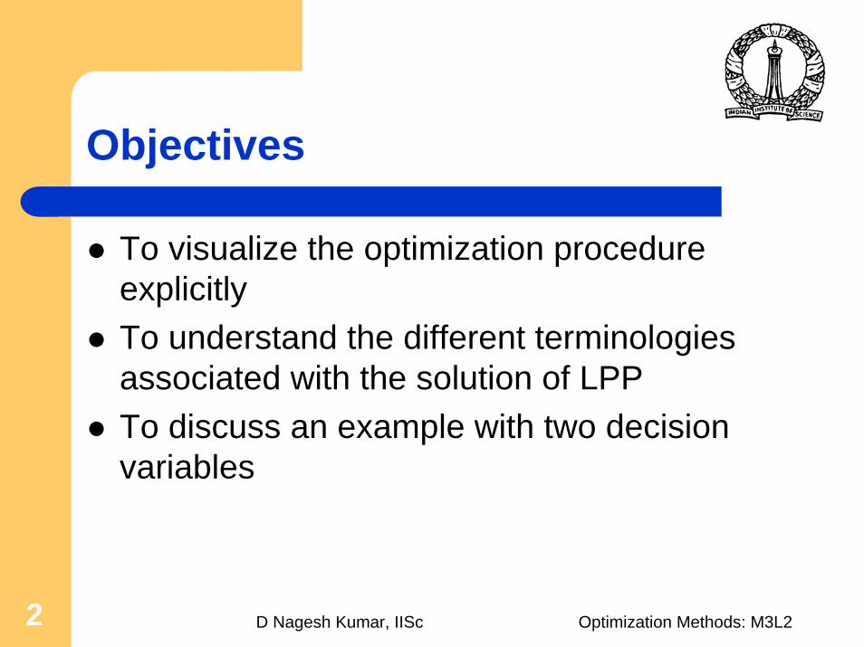
To visualize the optimization procedure explicitly To understand the different terminologies associated with the solution of LPP To discuss an example with two decision variables

D Nagesh Kumar, IISc Optimization Methods: M3L23

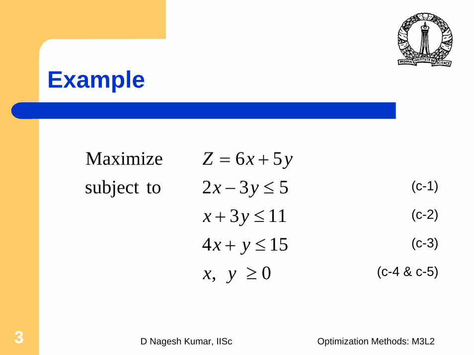
Example

(c-1)

(c-2)

(c-3)

(c-4 & c-5)0,154113

532tosubject56Maximize

≥≤+≤+≤−+=

yxyxyxyx

yxZ

D Nagesh Kumar, IISc Optimization Methods: M3L24

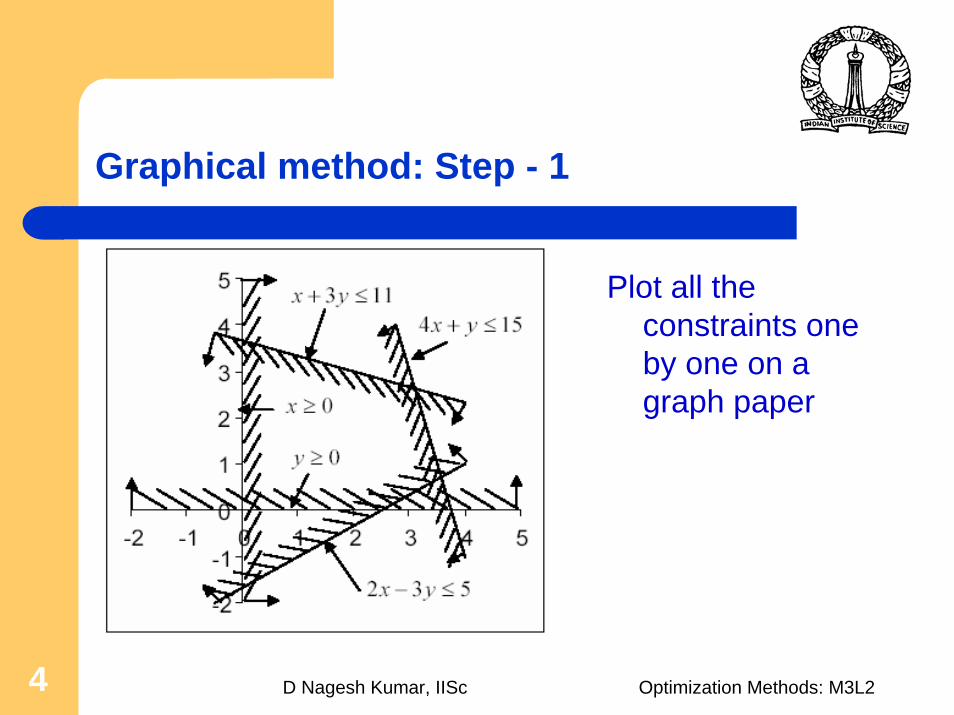
Graphical method: Step - 1

Plot all the constraints one by one on a graph paper

D Nagesh Kumar, IISc Optimization Methods: M3L25

Graphical method: Step - 2

Identify the common region of all the constraints.

This is known as ‘feasible region’

D Nagesh Kumar, IISc Optimization Methods: M3L26

Graphical method: Step - 3

Plot the objective function assuming any constant, k, i.e.

This is known as ‘Z line’, which can be shifted perpendicularly by changing the value of k.

kyx =+ 56

D Nagesh Kumar, IISc Optimization Methods: M3L27

Graphical method: Step - 4

Notice that value of the objective function will be maximum when it passes through the intersection of and (straight lines associated with 2nd

and 3rd constraints).This is known as ‘Optimal

Point’

113 =+ yx154 =+ yx

D Nagesh Kumar, IISc Optimization Methods: M3L28

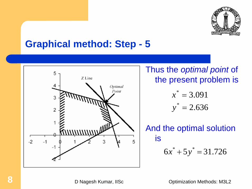
Graphical method: Step - 5

Thus the optimal point of the present problem is

And the optimal solution is

31.726 56 ** =+ yx

091.3* =x636.2* =y

D Nagesh Kumar, IISc Optimization Methods: M3L29

Different cases of optimal solution

A linear programming problem may have

1. A unique, finite solution (example already discussed)

2. An unbounded solution,

3. Multiple (or infinite) number of optimal solution,

4. Infeasible solution, and

5. A unique feasible point.

D Nagesh Kumar, IISc Optimization Methods: M3L210

Unbounded solution: Graphical representation

Situation: If the feasible region is not bounded

Solution: It is possible that the value of the objective function goes on increasing without leaving the feasible region, i.e., unbounded solution

D Nagesh Kumar, IISc Optimization Methods: M3L211

Multiple solutions: Graphical representation

Situation: Z line is parallel to any side of the feasible region

Solution: All the points lying on that side constitute optimal solutions

D Nagesh Kumar, IISc Optimization Methods: M3L212

Infeasible solution: Graphical representation

Situation: Set of constraints does not form a feasible region at all due to inconsistency in the constraints

Solution: Optimal solution is not feasible

D Nagesh Kumar, IISc Optimization Methods: M3L213

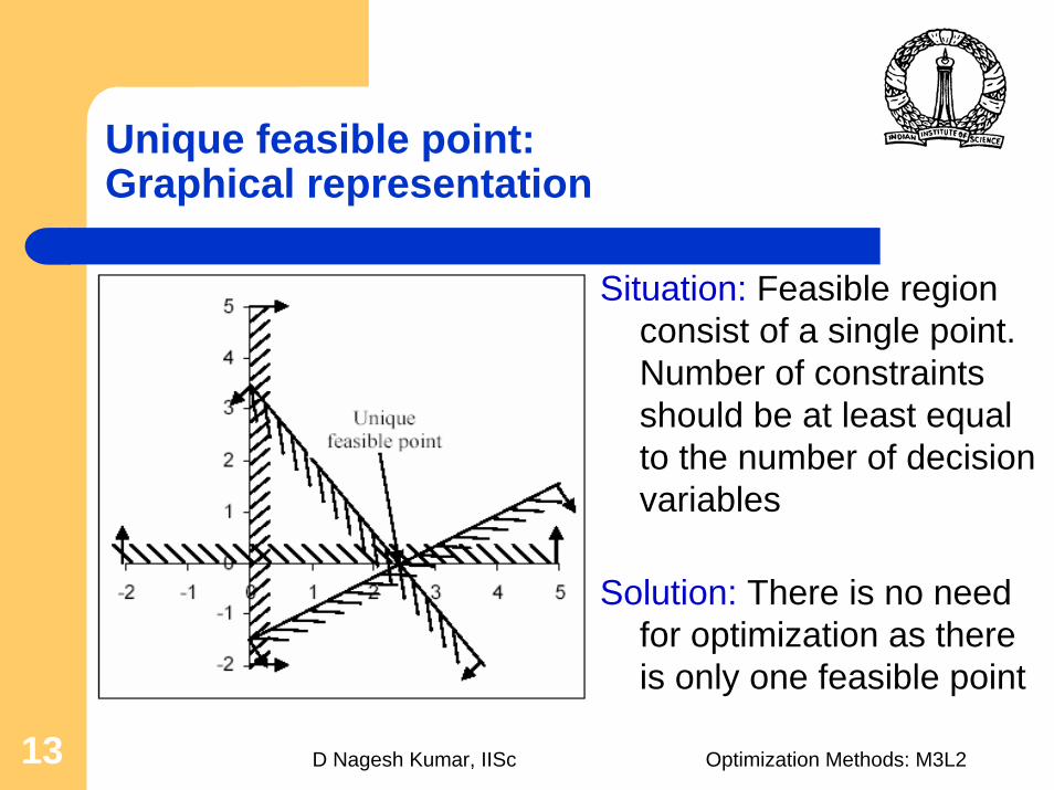
Unique feasible point: Graphical representation

Situation: Feasible region consist of a single point. Number of constraints should be at least equal to the number of decision variables

Solution: There is no need for optimization as there is only one feasible point

D Nagesh Kumar, IISc Optimization Methods: M3L214

Thank You