Linear mixed model for heritability estimation thatexplicitly addresses environmental variationDavid Heckermana,1, Deepti Gurdasanib,c, Carl Kadied, Cristina Pomillab,c, Tommy Carstensenb,c, Hilary Martinb,Kenneth Ekorub,c, Rebecca N. Nsubugae, Gerald Ssenyomoe, Anatoli Kamalie, Pontiano Kaleebue, Christian Widmera,and Manjinder S. Sandhub,c

aMicrosoft Research, Los Angeles, CA 90024; bWellcome Trust Sanger Institute, Hinxton CB10 1SA, United Kingdom; cDepartment of Medicine, Universityof Cambridge, Cambridge CB2 0SP, United Kingdom; dMicrosoft Research, Redmond, WA 98052; and eMRC/UVRI Uganda Research Unit onAIDS, Uganda

Edited by Richard M. Shiffrin, Indiana University, Bloomington, IN, and approved April 8, 2016 (received for review July 9, 2015)

The linear mixed model (LMM) is now routinely used to estimateheritability. Unfortunately, as we demonstrate, LMM estimates ofheritability can be inflated when using a standard model. To helpreduce this inflation, we used a more general LMM with two randomeffects—one based on genomic variants and one based on easily mea-sured spatial location as a proxy for environmental effects. We inves-tigated this approach with simulated data and with data from aUganda cohort of 4,778 individuals for 34 phenotypes including anthro-pometric indices, blood factors, glycemic control, blood pressure, lipidtests, and liver function tests. For the genomic random effect, weused identity-by-descent estimates from accurately phased genome-wide data. For the environmental random effect, we constructed acovariance matrix based on a Gaussian radial basis function. Acrossthe simulated and Ugandan data, narrow-sense heritability estimateswere lower using the more general model. Thus, our approach ad-dresses, in part, the issue of “missing heritability” in the sense thatmuch of the heritability previously thought to bemissingwas fictional.Software is available at https://github.com/MicrosoftGenomics/FaST-LMM.

heritability estimation | linear mixed model | environment |Gaussian radial basis function | model misspecification

An important causal question comes from the age-old debateabout nature versus nurture. For any phenotype such as height

or intelligence quotient, how much of the phenotype is inheritedand how much is determined by environment? This question wasmade precise by Fisher (1) and Wright (2) almost a century ago:Given observations of a phenotype from a population of individuals,what is the fraction of variance of the phenotype that is caused byinherited factors relative to the total variance of the phenotype dueto both inherited and environmental factors? This fraction, termed“heritability,” has been the subject of intense study across variousphenotypes and populations since it was defined. Note that, incontrast to how some interpret the informal question around thenature-versus-nurture debate, heritability is not an absolute quantitybut rather a quantity relative to a given population. For example, aphenotype in a population where environmental factors have largevariation will have a smaller heritability than in an otherwise similarpopulation where environmental factors have a small variation.Over the years, many approaches have been developed to estimate

heritability from data (3, 4). Here, we concentrate on an approachmade possible by the recent ability to sequence genomes at a modestcost (5, 6). The approach uses a linear mixed model (LMM), a formof multivariate regression of the genomic and environmental factorson the phenotype, which we examine in detail in the next section.In the standard LMM approach, the effects of environmental

factors on the phenotype are modeled as noise. Specifically, thephenotype of each individual is assumed to be the sum of tworandom effects, one based on genomic factors and one based onenvironmental factors, where the latter is assumed to be mutuallyindependent across individuals. As we shall see, this model forenvironmental effects can lead to inflated estimates of heritability.

To avoid this inflation, we could measure and model envi-ronmental effect explicitly (e.g., ref. 7). Unfortunately, in mostcircumstances there are many environmental factors to be mea-sured. Furthermore, some environmental factors may be un-recognized and consequently are unmeasurable. In this work, weinvestigate the use of an easy-to-measure surrogate for environ-mental factors—namely, spatial location. We show how this surro-gate can be incorporated into the LMM as an additional randomeffect. We investigate our more general model with simulated dataand with data from a Ugandan cohort of about 5,000 individuals.

ResultsHeritability Estimation. First, let us consider a standard approachfor estimating heritability using an LMM (6, 8). The estimate isbased on observations consisting of y, an N × 1 vector of phe-notypes for the N individuals, and X, an N ×M matrix of causalgenomic variants for the N individuals and M variants. Note thatit is customary to normalize the causal variants so that eachone has a mean of zero and an SD of one across individuals.Given these observations, we model y as a multivariate linearregression on X:

y∼N �μ+Xβ;σ2r I�, [1]

where μ is an N × 1 vector of offsets that can include the effectsof covariates, β is the M × 1 vector of linear weights relating thecorresponding variants to the phenotype, I is the N ×N identitymatrix, and σ2r is the residual variance of the multivariate normaldistribution denoted by N (.; .). In addition, we assume that theelements of β are mutually independent, each having a normaldistribution:

βi ∼N 0; 

σ2gM

!,   i= 1, . . . ,  M. [2]

This paper results from the Arthur M. Sackler Colloquium of the National Academy ofSciences, “Drawing Causal Inference from Big Data,” held March 26–27, 2015, at theNational Academies of Sciences in Washington, DC. The complete program and videorecordings of most presentations are available on the NAS website at www.nasonline.org/Big-data.

Author contributions: D.H., D.G., C.K., C.W., and M.S.S. designed research; D.H., D.G., C.K.,C.P., T.C., H.M., K.E., R.N.N., G.S., A.K., P.K., C.W., and M.S.S. performed research; D.H.,C.K., and C.W. contributed new reagents/analytic tools; D.H., D.G., C.K., C.W., and M.S.S.analyzed data; and D.H., D.G., C.K., C.W., and M.S.S. wrote the paper.

Conflict of interest statement: D.H., C.K., and C.W. were employees of Microsoft Researchwhile performing this research.

This article is a PNAS Direct Submission.

Data deposition: The genomic data have been deposited at the European Genome-phenome Archive (EGA, https://www.ebi.ac.uk/ega/) (accession no. EGAS00001001558).1To whom correspondence should be addressed. Email: heckerma@microsoft.com.

This article contains supporting information online at www.pnas.org/lookup/suppl/doi:10.1073/pnas.1510497113/-/DCSupplemental.

www.pnas.org/cgi/doi/10.1073/pnas.1510497113 PNAS | July 5, 2016 | vol. 113 | no. 27 | 7377–7382

GEN

ETICS

STATIST

ICS

COLLOQUIUM

PAPE

R

Plugging Eq. 2 into Eq. 1 and integrating out β, we obtain

y∼N�μ;σ2g

1M

XXT + σ2r I�. [3]

Model 3 is known as a linear mixed model with a random effecthaving the covariance matrix Kcausal = 1

M XXT (9). It is also knownas a Gaussian process with a linear covariance (or kernel) function(10, 11). Note that element i,j of Kcausal is the dot productPMk=1

XikXjk. The parameters of this model are typically fit by maxi-

mizing the restricted maximum likelihood (REML) of the data.Narrow sense heritability, denoted h2, is the fraction of the

variance of y due to the genomic component. Given this model andthe assumption that genomic variants are mutually independent, itfollows that

h2 =σ2g  

σ2g + σ2r. [4]

Note that narrow-sense heritability accounts only for additivegenomic effects. Genomic effects can also exhibit nonlinear inter-actions among each other (known as epistasis) and exhibitdominance, neither of which is captured in the model of Eq. 3. Theterm “heritability” without the modifier “narrow sense” is typicallyreserved for the quantity that includes all genomic effects. Herein,for simplicity, we will concentrate on the estimation of narrow-senseheritability although, as we mention later, our approach can beextended to estimate more general quantities.In practice, we do not know which genomic variants are causal,

so we use an approximation for Kcausal. One commonly usedapproximation—and one we will use in this work—is KIBD, whereelement (i,j) is the fraction of the genome shared identical by de-scent (IBD) among individuals i and j (6). That is, we use the model

y∼N�μ;σ2gKIBD + σ2r I

�.

As noted in the introduction, the standard LMM representsenvironmental effects as simple Gaussian noise. Here, let usconsider a more general model for environmental effects basedon the spatial location of individuals. Specifically, consider theaddition of a random effect with covariance matrix Kloc:

y∼N�μ;σ2gKIBD + σ2eKloc + σ2r I

�. [5]

Assuming the genomic variants and spatial locations aremutually independent, we get a new estimate for narrow-senseheritability given by

h2 =σ2g  

σ2g + σ2e + σ2r. [6]

This model also allows us to estimate the fraction of variance of ydue to the location component, denoted e2:

e2 =σ2e  

σ2g + σ2e + σ2r. [7]

In our analysis of the Ugandan cohort, we use Klocði, jÞ=expf−ðdij=αÞ2g, where dij is the distance between individuals iand j, and α is a scaling parameter. Intuitively, the inclusion ofKloc captures the notion that individuals physically closer to eachother are more likely to be influenced by the same environmentalfactors and hence more likely to have similar phenotypes. Usingother types of proximity—for example, social proximity—is alsopossible, but here we consider only physical proximity. The expo-nential form we use for Klocði, jÞ is known as a Gaussian radial

basis function and is often used in spatial analyses (10, 11). (Wealso tried the radial basis function expf−ðdij=αÞg but found it diffi-cult to estimate α accurately.) The parameter α can be thought of asthe spatial range of the environmental effect. The larger the valuefor α, the larger the range or extent of the effect. As in the standardcase, we fit all parameters, now including σ2e and α, with REML.Recall that the standard LMM follows from modeling the phe-

notype as a regression on genomic variants. Similarly, Eq. 5 can beinterpreted as the result of modeling the phenotype as a multivariateregression on both genomic variants and spatial location. In par-ticular, Mercer’s theorem (10, 11) states that, if K(zi,zj) is a contin-uous symmetric positive semidefinite function to R from zi and zjeach in a compact Hausdorff space, then there exists a set offunctions ϕk(z), k = 1,. . .,∞, such that K(zi,zj) is equal to the

dot productP∞k=1

ϕkðziÞϕkðzjÞ. Identifying zi as the spatial location

of individual i and K(zi,zj) as element i,j in Kloc, it follows that theinclusion of Kloc in Eq. 5 is equivalent to conditioning on spatialfeatures ϕk(zi), i = 1,. . .,N, k = 1,. . .,∞. We note that the Gaussianradial basis function is guaranteed to be positive semidefinite.Finally, let us consider nonlinear interactions between genomic

and environmental components. We can model some of these in-teractions by introducing a third random effect to the LMM:

y∼N�μ;σ2gKIBD + σ2eKloc + σ2gxeKGxE + σ2r I

�, [8]

producing an estimate of the fraction of variance of y due to theinteraction component given by

gxe2 =σ2gxe  

σ2g + σ2e + σ2gxe+ σ2r. [9]

We use a particular form for KGxE where element i,j is theproduct of elements i,j from Kcausal and Kloc (i.e., the Handa-mard product of Kcausal and Kloc). Using the nomenclature wehave defined, it follows that element i,j of  KGxE is given byPMk=1

P∞l=1

XikϕlðziÞXjkϕlðzjÞ. Consequently, inclusion of KGxE into

the LMM is equivalent to conditioning on the features Xik ϕl(zi),i = 1,. . .,N, k = 1,. . .,M, l = 1,. . .,∞. Product features such asthese are often used to model nonlinear interactions (12). In ouranalysis of the Ugandan cohort, we use this instance of KGxE,except we replace Kcausal with KIBD as an approximation.We note that the standard model given by Eq. 3 is nested in the

model given by Eq. 5, which in turn is nested in the model givenby Eq. 8.

Heritability Analysis on Simulated Data. We first applied our ap-proach to the analysis of simulated data. We generated from theBalding–Nichols model (13) with a 50:50 population ratio, a baselineminor allele frequency (MAF) sampled uniformly from [0.05, 0.5],and a value for Wright’s FST equal to 0.1. We generated a spatiallocation for each individual by sampling randomly from one of twospherical Gaussian distributions with SD 625,000 and separationbetween Gaussian centers equal to 4 × 625,000. This procedureproduced a distribution of spatial locations similar to the real dataand satisfied an assumption underlying Eqs. 6 and 7 that genomicvariants and spatial locations are independent. We next generatedthe phenotype using Eq. 5 with KIBD replaced with Kcausal, and withσ2g = σ2e = σ2r = 1, and α = 4 × 625,000. We generated 50 datasetsand then, for each one, computed uncorrected and corrected heri-tability estimates, based on Eqs. 3 and 5, respectively, with KIBDreplaced with Kcausal. For each dataset, we generated 1,000 causalSNPs for 5,000 individuals to mimic the real data.The estimates of h2 and e2 based on the corrected model are

unbiased, having mean (± SE) of 0.33 ± 0.01 and 0.35 ± 0.02,respectively. In contrast, the estimates of h2 based on the standard

7378 | www.pnas.org/cgi/doi/10.1073/pnas.1510497113 Heckerman et al.

or uncorrected model were inflated (0.42 ± 0.01). This inflation isnot unexpected, because the “signal” produced by the spatial ran-dom effect needs to be accounted for by either the genomic randomeffect or the noise component, and there is no reason to expect thatthe noise component would account for all of it. Any leakage of thesignal arising from the spatial random effect to the genomic randomeffect would yield inflated estimates of heritability. That is, modelmisspecification can lead to substantial bias in heritability estimates.As mentioned, Eqs. 6 and 7 were derived under an assumption

that genomic and spatial factors are independent. In practice,however, this assumption may not hold. To investigate the ro-bustness of these estimates to nonindependence, we modified theabove data-generation procedure to create a dependence betweengenomic and spatial variation. In particular, the spatial locations ofall individuals from the same Balding–Nichols population weredrawn from the same spherical Gaussian. Despite this relativelystrong dependence, estimates of h2 (corrected) and e2 remainedunbiased (0.33 ± 0.01 and 0.35 ± 0.02, respectively). Uncorrectedestimates of h2 were similarly inflated in the presence of de-pendence (0.46 ± 0.01).Sample code for these experiments in the form of an iPython

notebook can be found in SI Appendix.

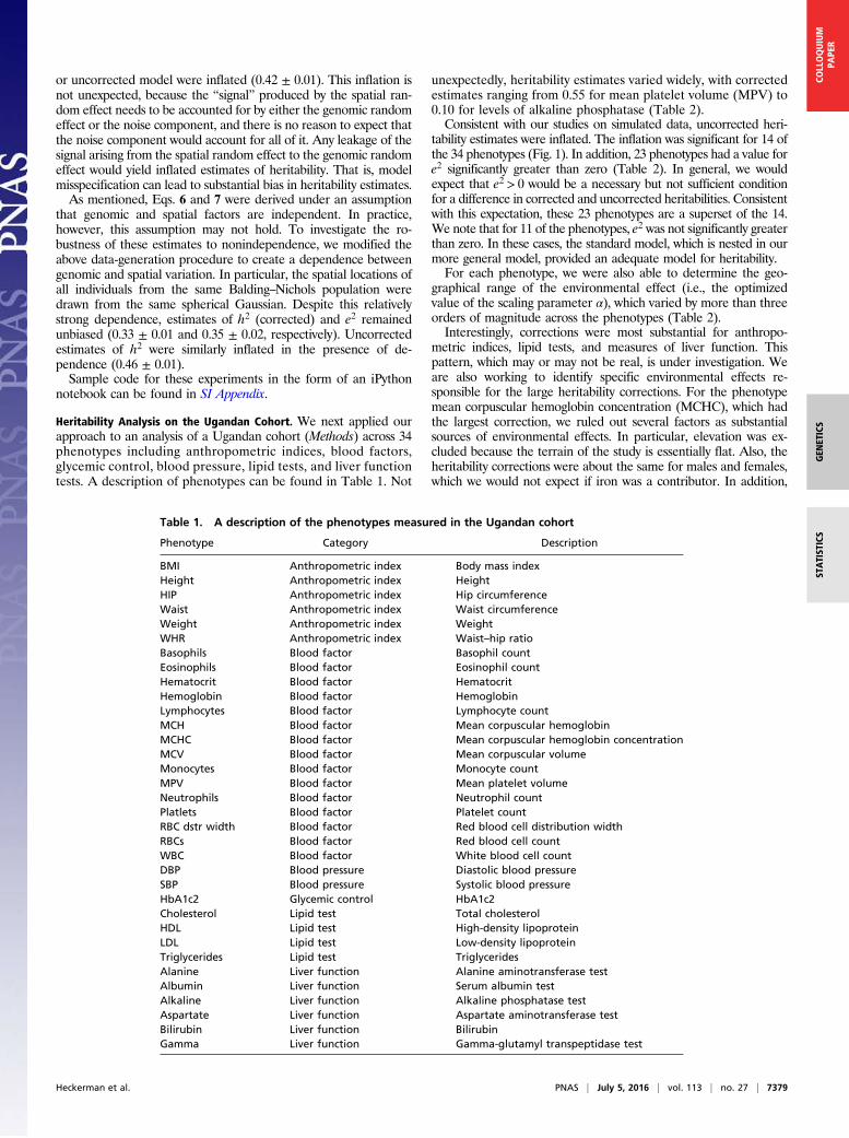
Heritability Analysis on the Ugandan Cohort. We next applied ourapproach to an analysis of a Ugandan cohort (Methods) across 34phenotypes including anthropometric indices, blood factors,glycemic control, blood pressure, lipid tests, and liver functiontests. A description of phenotypes can be found in Table 1. Not

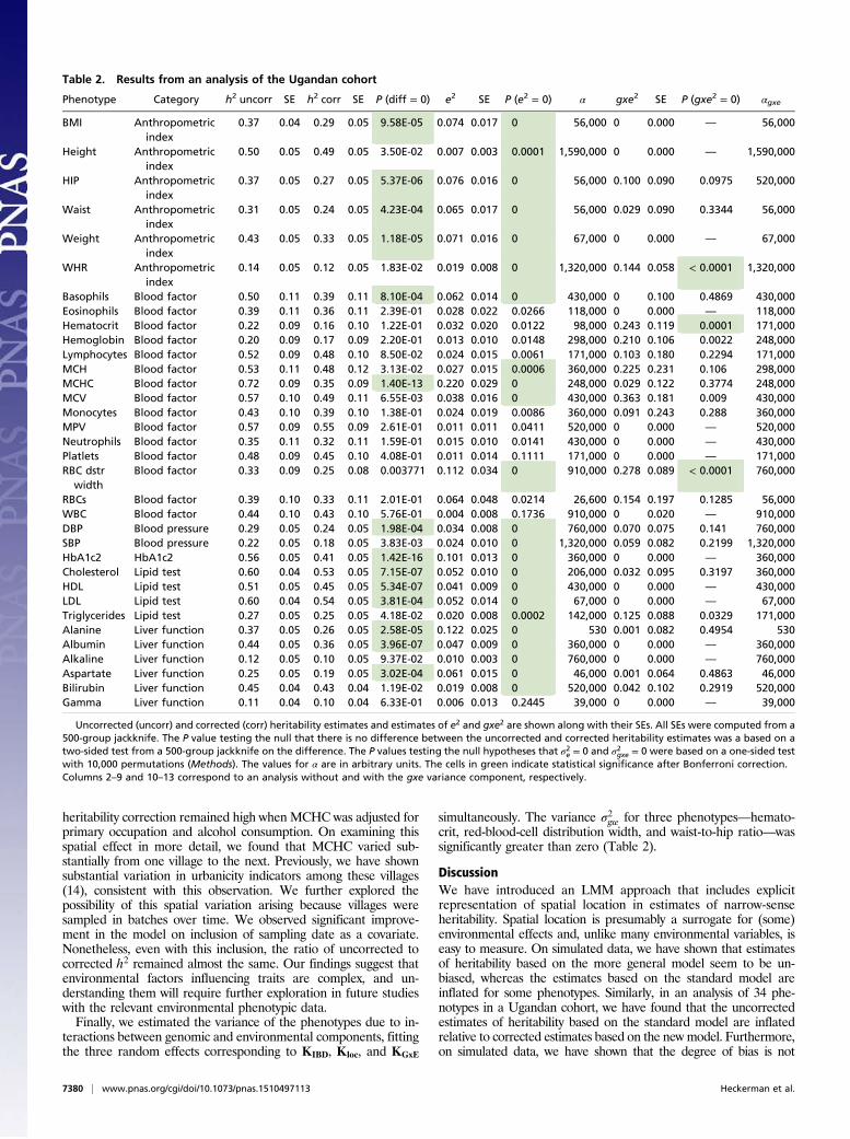
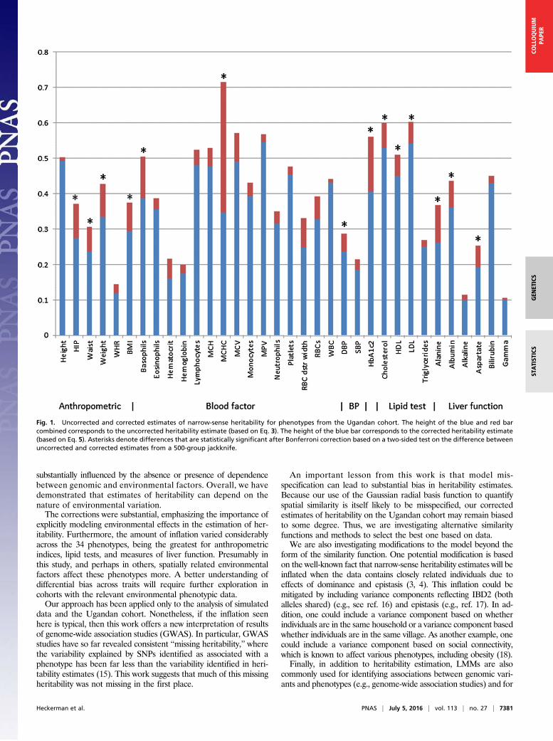
unexpectedly, heritability estimates varied widely, with correctedestimates ranging from 0.55 for mean platelet volume (MPV) to0.10 for levels of alkaline phosphatase (Table 2).Consistent with our studies on simulated data, uncorrected heri-

tability estimates were inflated. The inflation was significant for 14 ofthe 34 phenotypes (Fig. 1). In addition, 23 phenotypes had a value fore2 significantly greater than zero (Table 2). In general, we wouldexpect that e2 > 0 would be a necessary but not sufficient conditionfor a difference in corrected and uncorrected heritabilities. Consistentwith this expectation, these 23 phenotypes are a superset of the 14.We note that for 11 of the phenotypes, e2 was not significantly greaterthan zero. In these cases, the standard model, which is nested in ourmore general model, provided an adequate model for heritability.For each phenotype, we were also able to determine the geo-

graphical range of the environmental effect (i.e., the optimizedvalue of the scaling parameter α), which varied by more than threeorders of magnitude across the phenotypes (Table 2).Interestingly, corrections were most substantial for anthropo-

metric indices, lipid tests, and measures of liver function. Thispattern, which may or may not be real, is under investigation. Weare also working to identify specific environmental effects re-sponsible for the large heritability corrections. For the phenotypemean corpuscular hemoglobin concentration (MCHC), which hadthe largest correction, we ruled out several factors as substantialsources of environmental effects. In particular, elevation was ex-cluded because the terrain of the study is essentially flat. Also, theheritability corrections were about the same for males and females,which we would not expect if iron was a contributor. In addition,

Table 1. A description of the phenotypes measured in the Ugandan cohort

Phenotype Category Description

BMI Anthropometric index Body mass indexHeight Anthropometric index HeightHIP Anthropometric index Hip circumferenceWaist Anthropometric index Waist circumferenceWeight Anthropometric index WeightWHR Anthropometric index Waist–hip ratioBasophils Blood factor Basophil countEosinophils Blood factor Eosinophil countHematocrit Blood factor HematocritHemoglobin Blood factor HemoglobinLymphocytes Blood factor Lymphocyte countMCH Blood factor Mean corpuscular hemoglobinMCHC Blood factor Mean corpuscular hemoglobin concentrationMCV Blood factor Mean corpuscular volumeMonocytes Blood factor Monocyte countMPV Blood factor Mean platelet volumeNeutrophils Blood factor Neutrophil countPlatlets Blood factor Platelet countRBC dstr width Blood factor Red blood cell distribution widthRBCs Blood factor Red blood cell countWBC Blood factor White blood cell countDBP Blood pressure Diastolic blood pressureSBP Blood pressure Systolic blood pressureHbA1c2 Glycemic control HbA1c2Cholesterol Lipid test Total cholesterolHDL Lipid test High-density lipoproteinLDL Lipid test Low-density lipoproteinTriglycerides Lipid test TriglyceridesAlanine Liver function Alanine aminotransferase testAlbumin Liver function Serum albumin testAlkaline Liver function Alkaline phosphatase testAspartate Liver function Aspartate aminotransferase testBilirubin Liver function BilirubinGamma Liver function Gamma-glutamyl transpeptidase test

Heckerman et al. PNAS | July 5, 2016 | vol. 113 | no. 27 | 7379

GEN

ETICS

STATIST

ICS

COLLOQUIUM

PAPE

R

heritability correction remained high when MCHC was adjusted forprimary occupation and alcohol consumption. On examining thisspatial effect in more detail, we found that MCHC varied sub-stantially from one village to the next. Previously, we have shownsubstantial variation in urbanicity indicators among these villages(14), consistent with this observation. We further explored thepossibility of this spatial variation arising because villages weresampled in batches over time. We observed significant improve-ment in the model on inclusion of sampling date as a covariate.Nonetheless, even with this inclusion, the ratio of uncorrected tocorrected h2 remained almost the same. Our findings suggest thatenvironmental factors influencing traits are complex, and un-derstanding them will require further exploration in future studieswith the relevant environmental phenotypic data.Finally, we estimated the variance of the phenotypes due to in-

teractions between genomic and environmental components, fittingthe three random effects corresponding to KIBD, Kloc, and KGxE

simultaneously. The variance σ2gxe for three phenotypes—hemato-crit, red-blood-cell distribution width, and waist-to-hip ratio—wassignificantly greater than zero (Table 2).

DiscussionWe have introduced an LMM approach that includes explicitrepresentation of spatial location in estimates of narrow-senseheritability. Spatial location is presumably a surrogate for (some)environmental effects and, unlike many environmental variables, iseasy to measure. On simulated data, we have shown that estimatesof heritability based on the more general model seem to be un-biased, whereas the estimates based on the standard model areinflated for some phenotypes. Similarly, in an analysis of 34 phe-notypes in a Ugandan cohort, we have found that the uncorrectedestimates of heritability based on the standard model are inflatedrelative to corrected estimates based on the newmodel. Furthermore,on simulated data, we have shown that the degree of bias is not

Table 2. Results from an analysis of the Ugandan cohort

Uncorrected (uncorr) and corrected (corr) heritability estimates and estimates of e2 and gxe2 are shown along with their SEs. All SEs were computed from a500-group jackknife. The P value testing the null that there is no difference between the uncorrected and corrected heritability estimates was a based on atwo-sided test from a 500-group jackknife on the difference. The P values testing the null hypotheses that σ2e = 0 and σ2gxe = 0 were based on a one-sided testwith 10,000 permutations (Methods). The values for α are in arbitrary units. The cells in green indicate statistical significance after Bonferroni correction.Columns 2–9 and 10–13 correspond to an analysis without and with the gxe variance component, respectively.

7380 | www.pnas.org/cgi/doi/10.1073/pnas.1510497113 Heckerman et al.

substantially influenced by the absence or presence of dependencebetween genomic and environmental factors. Overall, we havedemonstrated that estimates of heritability can depend on thenature of environmental variation.The corrections were substantial, emphasizing the importance of

explicitly modeling environmental effects in the estimation of her-itability. Furthermore, the amount of inflation varied considerablyacross the 34 phenotypes, being the greatest for anthropometricindices, lipid tests, and measures of liver function. Presumably inthis study, and perhaps in others, spatially related environmentalfactors affect these phenotypes more. A better understanding ofdifferential bias across traits will require further exploration incohorts with the relevant environmental phenotypic data.Our approach has been applied only to the analysis of simulated

data and the Ugandan cohort. Nonetheless, if the inflation seenhere is typical, then this work offers a new interpretation of resultsof genome-wide association studies (GWAS). In particular, GWASstudies have so far revealed consistent “missing heritability,” wherethe variability explained by SNPs identified as associated with aphenotype has been far less than the variability identified in heri-tability estimates (15). This work suggests that much of this missingheritability was not missing in the first place.

An important lesson from this work is that model mis-specification can lead to substantial bias in heritability estimates.Because our use of the Gaussian radial basis function to quantifyspatial similarity is itself likely to be misspecified, our correctedestimates of heritability on the Ugandan cohort may remain biasedto some degree. Thus, we are investigating alternative similarityfunctions and methods to select the best one based on data.We are also investigating modifications to the model beyond the

form of the similarity function. One potential modification is basedon the well-known fact that narrow-sense heritability estimates will beinflated when the data contains closely related individuals due toeffects of dominance and epistasis (3, 4). This inflation could bemitigated by including variance components reflecting IBD2 (bothalleles shared) (e.g., see ref. 16) and epistasis (e.g., ref. 17). In ad-dition, one could include a variance component based on whetherindividuals are in the same household or a variance component basedwhether individuals are in the same village. As another example, onecould include a variance component based on social connectivity,which is known to affect various phenotypes, including obesity (18).Finally, in addition to heritability estimation, LMMs are also

commonly used for identifying associations between genomic vari-ants and phenotypes (e.g., genome-wide association studies) and for

Fig. 1. Uncorrected and corrected estimates of narrow-sense heritability for phenotypes from the Ugandan cohort. The height of the blue and red barcombined corresponds to the uncorrected heritability estimate (based on Eq. 3). The height of the blue bar corresponds to the corrected heritability estimate(based on Eq. 5). Asterisks denote differences that are statistically significant after Bonferroni correction based on a two-sided test on the difference betweenuncorrected and corrected estimates from a 500-group jackknife.

Heckerman et al. PNAS | July 5, 2016 | vol. 113 | no. 27 | 7381

GEN

ETICS

STATIST

ICS

COLLOQUIUM

PAPE

R

prediction. The LMM models described in this work could be ap-plied to these applications as well.

MethodsWe collected data for 5,000 individuals from nine ethnolinguistic groups fromthe General Population Cohort (GPC), Uganda (19). The GPC is a population-based open cohort study established in 1989 by the Medical Research Council incollaboration with the Uganda Virus Research Institute (UVRI) to examinetrends in prevalence and incidence of HIV infection and their determinants.Samples were collected from individuals during a survey from the study arealocated in southwestern Uganda in Kyamulibwa subcounty of Kalungu district,∼120 km from Entebbe town. The study area is divided into villages defined byadministrative boundaries varying in size from 300 to 1,500 residents and in-cludes families living within households. Data on health and lifestyle werecollected using a standard individual questionnaire, blood samples obtained,and biophysical measurements taken, when necessary, as described previously(19). Spatial location was recorded in Global Positioning System coordinates.The measurements were translated and scaled to mitigate privacy concerns.

The GPC study was approved by the Uganda Virus Research Institute, Scienceand Ethics Committee (Ref. GC/127/10/10/25), the Uganda National Council forScience and Technology (Ref. HS 870), and the U.K. National Research EthicsService, Research Ethics Committee (Ref. 11/H0305/5). Care was taken to obtaingenuine informed consent from participants, including the use of reliableintermediaries as appropriate to ensure that the implications of participationwere fully understood. Consent forms were translated from English into Lu-ganda and checked for accuracy. The Lugandan translation was given to par-ticipants to read themselves, or was read out aloud to them by study staff.Participants could choose to consent to all, or just selected parts, of the survey.The informed consent of participants was obtained with a signature on theconsent forms or a thumb print if the participant was unable to write. Forparticipants aged 13–17 y, parental consent as well as child formal assent werecollected. The immediate counter signature of a witness was then obtained.The APCDR committees are responsible for curation, storage, and sharing ofthe data under managed access. The genomic data have been deposited at theEuropean Genome-phenome Archive (EGA, https://www.ebi.ac.uk/ega/) underaccession number EGAS00001001558. Requests for access to phenotype datamay be directed to data@apcdr.org.

We genotyped 5,000 samples from the Ugandan Survey on the IlluminaHumanOmni 2.5M BeadChip array at the Wellcome Trust Sanger Institute.Sequenom quality control and gender checks were carried out before geno-typing. A total of 2,314,174 autosomal and 55,208 X-chromosomemarkers weregenotyped on the HumanOmni2.5–8 chip. Of these, 39,368 autosomal markerswere excluded because they did not pass the quality thresholds for the SNPcalled proportion (<97%, 25,037 SNPs) and Hardy–Weinberg equilibrium (HWE)(P < 10−8, 14,331 SNPs). HWE testing was only carried out on the founders forautosomes, and female unrelated individuals for the X chromosome defined byan IBD threshold <0.10 as estimated by PLINK. A total of 91 samples weredropped during sample quality control because they did not pass the qualitythresholds for proportion of samples called (>97%) or heterozygosity (outliers:

mean ± 3 SD), or the gender inferred from the X-chromosome data did notmatch the supplied gender. Three additional samples were dropped because ofhigh relatedness (i.e., IBD >0.90). Principal component analysis was carried outon unrelated individuals projecting onto related individuals, for SNPs LD prunedat an r2 threshold of 0.2, with a MAF threshold of >5%. No samples wereidentified as population/ancestry outliers based on this analysis.

To generate the phased dataset, we first mapped pedigrees within ourdataset based on relationships provided in the data. To detect any errors in thesepedigrees, we ran KING (20) on each cohort and also used the results to identifyany cryptic first-degree relationships that had not been mapped. We furtherremoved pedigrees where age information was inconsistent with the pedigreespecified. In addition to the quality control described, we also removed SNPswith a minor allele frequency in the founders less than 5%, or with more than1%Mendelian errors. We set all remaining Mendelian errors to missing, as wellas any genotypes flagged as unlikely by the detection algorithm Merlin (21).SNPs with more than 1% missingness were then removed. We phased this cu-rated dataset of 1,340,101 SNPs using SHAPEIT2 (22), first phasing the samplesignoring family information, and then running a hidden Markov model onevery parent–child duo. This procedure corrects phasing errors inconsistent withthe pedigree structure, further improving phasing accuracy. We have previouslyshown this method produces highly accurate results in our cohort with negli-gible switch error rates (22). To construct KIBD from these phased data, we usedthe method outlined in ref. 23.

Phenotypes were transformed before analysis. Residuals were obtained fol-lowing regression of the trait on age, age squared, and sex. Residuals were theninverse-normally transformed for analysis. For HbA1c, regression was carried outonage, age squared, sex, andmonthof sample collection (as an indicator variable)to account for seasonal trends in HbA1C that have been described previously (24).

Heritability estimationwas performedwith the FaST-LMMtoolset available athttps://github.com/MicrosoftGenomics/FaST-LMM. To determine a P value forthe null hypothesis σ2e = 0, we performed a permutation test wherein the en-tries of Kloc were permuted by randomly shuffling the identifiers of the indi-viduals. A P value for the null hypothesis σ2gxe = 0 was determined similarly bypermuting the entries of KGxE. In both cases, 10,000 permutations were used.

ACKNOWLEDGMENTS. We thank Christoph Lippert for discussions aboutMercer’s theorem, Noah Zaitlen for discussions about more general modelsfor heritability estimation, Ashish Kapoor for discussions on how best to fitthe scaling parameters for radial basis functions, and Johanna Riha for discus-sions regarding the sources of spatial variance for some phenotypes. We thankthe African Partnership for Chronic Disease Research for providing a network tosupport this study as well as a repository for deposition of curated data.We alsothank all study participants who contributed to this study and the NationalInstitute of Health Research Cambridge Biomedical Research Centre for datacollection and phenotype analysis. This work was funded by the WellcomeTrust, Wellcome Trust Sanger Institute Grant WT098051, Medical ResearchCouncil Grants G0901213-92157, G0801566, and MR/K013491/1, and the Med-ical Research Council/Uganda Virus Research Institute Uganda Research Unit onAIDS core funding.

1. Fisher RA (1918) The correlation between relatives on the supposition of Mendelianinheritance. Trans R Soc Edinb 52:399–433.

2. Wright S (1920) The relative importance of heredity and environment in determiningthe piebald pattern of guinea-pigs. Proc Natl Acad Sci USA 6(6):320–332.

3. Falconer DS,Mackay TFC (1996) Introduction toQuantitative Genetics (Longman, Harlow, UK).4. LynchM,Walsh B (1998)Genetics andAnalysis of Quantitative Traits (Sinauer, Sunderland,MA).5. National Genome Human Research Institute (2015) National Genome Human Re-

search Institute. Available at https://www.genome.gov/.6. Zaitlen N, Kraft P (2012) Heritability in the genome-wide association era. Hum Genet

131(10):1655–1664.7. Valdar W, et al. (2006) Genetic and environmental effects on complex traits in mice.

Genetics 174(2):959–984.8. Yang J, et al. (2010) Common SNPs explain a large proportion of the heritability for

human height. Nat Genet 42(7):565–569.9. Hayes BJ, Visscher PM, Goddard ME (2009) Increased accuracy of artificial selection by

using the realized relationship matrix. Genet Res 91(1):47–60.10. Bernhard S, Smola AJ (2001) Learning with Kernels (MIT Press, Cambridge, MA).11. Rasmussen CE, Williams CKI (2006) Gaussian Processes for Machine Learning (MIT

Press, Cambridge, MA).12. Cordell HJ (2002) Epistasis: What it means, what it doesn’t mean, and statistical

methods to detect it in humans. Hum Mol Genet 11(20):2463–2468.13. Balding DJ, Nichols RA (1995) A method for quantifying differentiation between

populations at multi-allelic loci and its implications for investigating identity andpaternity. Genetica 96(1-2):3–12.

14. Riha J, et al. (2014) Urbanicity and lifestyle risk factors for cardiometabolic diseases in

rural Uganda: A cross-sectional study. PLoS Med 11(7):e1001683.15. Eichler EE, et al. (2010) Missing heritability and strategies for finding the underlying

causes of complex disease. Nat Rev Genet 11(6):446–450.16. Zaitlen N, et al. (2013) Using extended genealogy to estimate components of heri-

tability for 23 quantitative and dichotomous traits. PLoS Genet 9(5):e1003520.17. Stern MP, et al. (1996) Evidence for linkage of regions on chromosomes 6 and 11 to

plasma glucose concentrations in Mexican Americans. Genome Res 6(8):724–734.18. Christakis NA, Fowler JH (2007) The spread of obesity in a large social network over 32

years. N Engl J Med 357(4):370–379.19. Asiki G, et al.; GPC team (2013) The general population cohort in rural south-

western Uganda: A platform for communicable and non-communicable disease

studies. Int J Epidemiol 42(1):129–141.20. Manichaikul A, et al. (2010) Robust relationship inference in genome-wide association

studies. Bioinformatics 26(22):2867–2873.21. Abecasis GR, Cherny SS, Cookson WO, Cardon LR (2002) Merlin–rapid analysis of

dense genetic maps using sparse gene flow trees. Nat Genet 30(1):97–101.22. O’Connell J, et al. (2014) A general approach for haplotype phasing across the full

spectrum of relatedness. PLoS Genet 10(4):e1004234.23. Price AL, et al. (2011) Single-tissue and cross-tissue heritability of gene expression via

identity-by-descent in related or unrelated individuals. PLoS Genet 7(2):e1001317.24. Tseng CL, et al. (2005) Seasonal patterns in monthly hemoglobin A1c values. Am

J Epidemiol 161(6):565–574.

7382 | www.pnas.org/cgi/doi/10.1073/pnas.1510497113 Heckerman et al.