Linear Light Source ReflectometryAndrew Gardner Chris Tchou Tim Hawkins Paul Debevec

University of Southern California Institute for Creative Technologies Graphics Laboratory1

ABSTRACTThis paper presents a technique for estimating the spatially-varyingreflectance properties of a surface based on its appearance duringa single pass of a linear light source. By using a linear light ratherthan a point light source as the illuminant, we are able to reliablyobserve and estimate the diffuse color, specular color, and specularroughness of each point of the surface. The reflectometry apparatuswe use is simple and inexpensive to build, requiring a single direc-tion of motion for the light source and a fixed camera viewpoint.Our model fitting technique first renders a reflectance table of howdiffuse and specular reflectance lobes would appear under movinglinear light source illumination. Then, for each pixel we compareits series of intensity values to the tabulated reflectance lobes todetermine which reflectance model parameters most closely pro-duce the observed reflectance values. Using two passes of the lin-ear light source at different angles, we can also estimate per-pixelsurface normals as well as the reflectance parameters. Additionallyour system records a per-pixel height map for the object and esti-mates its per-pixel translucency. We produce real-time renderingsof the captured objects using a custom hardware shading algorithm.We apply the technique to a test object exhibiting a variety of ma-terials as well as to an illuminated manuscript with gold lettering.To demonstrate the technique’s accuracy, we compare renderings ofthe captured models to real photographs of the original objects.

1 IntroductionVisual richness in computer-generated images can come from awide variety of sources: complex and interesting geometry; de-tailed and realistic texture maps, aesthetically designed and realis-tically simulated lighting, and expressive animation and dynamics.In recent years it has become possible to obtain many of these richqualities by sampling the properties of the real world: scanning 3Dobjects to obtain geometry, using digital images for texture maps,capturing real-world illumination, and using motion capture tech-niques to produce animation. What remains difficult is to acquirerealistic reflectance properties of real-world objects: their spatially-varying colors, specularities, roughnesses, and translucencies. Asa result, these properties are usually crafted laboriously by handusing image-editing software.

The problem of measuring object reflectance is well-understoodfor the case of a homogeneous material sample: a device called a

1USC ICT, 13274 Fiji Way 5th Floor, Marina del Rey, CA, 90292Email: gardner@ict.usc.edu, tchou@ict.usc.edu, timh@ict.usc.edu,paul@debevec.org. Videos and additional examples are available athttp://www.ict.usc.edu/graphics/LLS/

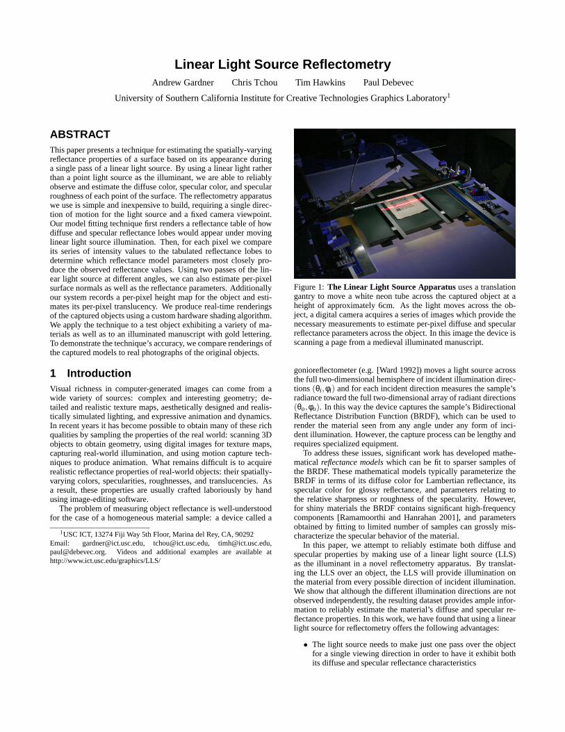
Figure 1:The Linear Light Source Apparatus uses a translationgantry to move a white neon tube across the captured object at aheight of approximately 6cm. As the light moves across the ob-ject, a digital camera acquires a series of images which provide thenecessary measurements to estimate per-pixel diffuse and specularreflectance parameters across the object. In this image the device isscanning a page from a medieval illuminated manuscript.

gonioreflectometer (e.g. [Ward 1992]) moves a light source acrossthe full two-dimensional hemisphere of incident illumination direc-tions(θi ,φi) and for each incident direction measures the sample’sradiance toward the full two-dimensional array of radiant directions(θo,φo). In this way the device captures the sample’s BidirectionalReflectance Distribution Function (BRDF), which can be used torender the material seen from any angle under any form of inci-dent illumination. However, the capture process can be lengthy andrequires specialized equipment.

To address these issues, significant work has developed mathe-matical reflectance modelswhich can be fit to sparser samples ofthe BRDF. These mathematical models typically parameterize theBRDF in terms of its diffuse color for Lambertian reflectance, itsspecular color for glossy reflectance, and parameters relating tothe relative sharpness or roughness of the specularity. However,for shiny materials the BRDF contains significant high-frequencycomponents [Ramamoorthi and Hanrahan 2001], and parametersobtained by fitting to limited number of samples can grossly mis-characterize the specular behavior of the material.

In this paper, we attempt to reliably estimate both diffuse andspecular properties by making use of a linear light source (LLS)as the illuminant in a novel reflectometry apparatus. By translat-ing the LLS over an object, the LLS will provide illumination onthe material from every possible direction of incident illumination.We show that although the different illumination directions are notobserved independently, the resulting dataset provides ample infor-mation to reliably estimate the material’s diffuse and specular re-flectance properties. In this work, we have found that using a linearlight source for reflectometry offers the following advantages:

• The light source needs to make just one pass over the objectfor a single viewing direction in order to have it exhibit bothits diffuse and specular reflectance characteristics

• The contrast ratio between the specular and diffuse peaks isreduced, allowing for standard digital imaging systems to ac-quire the reflectance data.

• The mechanics for moving a light source in just one dimen-sion are simple and inexpensive to build.

In the rest of this paper we describe the construction of ourLLS apparatus, and how we process the image data to derive spa-tially varying reflectance parameters for an object. Our device han-dles objects that are mostly planar, and we demonstrate the cap-ture technique on a flat test object as well as a medieval illumi-nated manuscript. We finally present a hardware-accelerated real-time rendering algorithm for the captured objects under novel il-lumination, and show that the technique realistically predicts thereflectance behavior of the objects under arbitrary point source illu-mination.

2 Background and Related WorkThe work in this paper relates to the general problem of creatingdigitized representations of real-world objects, and draws from awide variety of previous work in this area. The techniques can beroughly categorized as belonging to techniques for 3D scanning,reflectance modeling, reflectance measurement, and rendering.

Laser stripe systems such as those manufactured by Cyberware,Inc. have been used to acquire geometric models of mechanicalparts, sculptures, faces, and bodies. Techniques using structuredlight patterns and/or stereo correspondence techniques have beenused for geometry acquisition as well. A laser stripe system wasrecently used to scan Michaelangelo’s David [Levoy et al. 2000]and a structured light technique was used to scan his FlorentinePieta [Rushmeier et al. 1998]. [Halstead et al. 1996] used a differentapproach to geometry measurement by estimating the shape of theeye’s cornea from specular reflectance analysis. In our work, weuse a laser stripe technique for recording the non-planar geometryof our scanned objects and a specular reflectance analysis to recoversmaller-scale surface normal variations.

In reflectance modeling, Nicodemus et al [Nicodemus et al.1977] described how a surface transforms incident illuminationinto radiant illumination as its four-dimensional Bidirectional Re-flectance Distribution Function. Examples of BRDF models de-signed to be consistent with real-world reflectance properties areTorrance-Sparrow [Torrance and Sparrow 1967], Cook-Torrance[Cook and Torrance 1981], Poulin et al, [Poulin and Fournier 1990],Ward [Larson 1992], and Oren-Nayar [Oren and Nayar 1994].More recent work has proposed models which also consider thesubsurface scattering component of light reflection [Hanrahan andKrueger 1993; Jensen et al. 2001] for translucent surfaces. In ourwork, we make use of the Ward reflectance model [Larson 1992]with an additional simple translucency component.

Reflectance measurement, orreflectometry, has produced tech-niques for estimating the parameters of a reflectance model of real-world surfaces based on photographs of the surface under variouslighting conditions and viewing directions. For one example, theImage-Based BRDF measurement technique in [Marschner et al.1999] fitted cosine lobe [Lafortune et al. 1997] reflectance param-eters based on a small set of images of a convex material sam-ple. [Nayar et al. 1994] used pictures of an object illuminated bydifferent extended light sources to recover object shape, lamber-tian reflectance, and mirror-like specular reflectance. [Dana et al.1997] recorded spatially-varying BRDFs for various texture sam-ples using images of the sample rather than single radiance mea-surements. Another technique from [Marschner 1998] recorded aspatially-varying diffuse albedo map for a laser-scanned object byconsidering the visibility of each object surface to a moving light

source, and [Sato et al. 1997] in addition estimated uniform specu-lar reflectance parameters for an object by observing the intensity ofa specular lobe from various lighting directions. [Yu et al. 1999] es-timated spatially varying diffuse parameters and piecewise constantspecular parameters for images of a scene in a mutual illuminationcontext. [Debevec et al. 2000] used light sources positioned bothhorizontally and vertically around a person’s face to obtain spatiallyvarying parameters for both diffuse and specular reflection as wellas surface normals; [Malzbender et al. 2001] used an array of lightson the upper hemisphere to capture diffuse properties and surfacenormals of artifacts for real-time rendering. [Lensch et al. 2001]estimated spatially varying diffuse and specular properties makinguse of a principal component analysis of the possible reflectanceproperties of the object. [Zongker et al. 1999; Chuang et al. 2000]used patterns of light from behind an object on a video monitorto characterize the object’s reflectance functions for reflected andrefracted light.

[McAllister 2002] addressed the problem of capturing spatially-varying reflectance information for flat surfaces by directly record-ing and fitting the four-dimensional BRDF for each point on the ob-ject’s surface. Using a larger captured data set, pan and tilt robotics,and a least-squares BRDF-fitting method, the technique producedaccurate BRDF measurements including anisotropy, but at the costof relatively slow capture. In our work we use simpler equipmentand less data, additionally acquire surface normals, displacements,and translucency, but do not at this stage acquire anisotropy.

These previous techniques address important aspects of the re-flectometry problem for spatially-varying surfaces, but none is atonce general, efficient, and simple. In our work, we have foundthat using a linear light source as the illuminant allows us to effi-ciently capture both diffuse and specular properties using a simpletranslational gantry and fixed camera pose relative to the subject.

3 The Linear Light Source ApparatusIn this section we describe the design and construction of our Lin-ear Light Source reflectometry apparatus, including the linear lightsource, the translation gantry, the laser stripe, and the camera sys-tem.

The Linear Light Source (LLS) chosen for our device is awhite neon tube purchased from the automobile decoration com-pany Street Glow, Inc. for $20. The light runs on 12V DC andwas chosen over a fluorescent tube due to its low flicker and whiterspectrum, and over an incandescent light for its low heat output.The emissive light tube source was suitably small at 1cm in diame-ter and 50 cm long, and sits within a protective 2cm diameter clearplastic tube.

The spectrum of the white neon light tube is shown in Fig. 2. Thewhite ”neon” light produces light by exciting an argon-mercury gasmixture, which produces spectral emission lines in the ultraviolet,blue, green, and orange parts of the spectrum. The inside of thelight tube is coated with white phosphors which are excited by thehigher-frequency emission lines to produce energy across the vis-ible spectrum. The final emitted light also includes contributionsfrom the original Ar-Hg gas; for a future version we would like tofilter out these spectral peaks since they bias the recorded colorstoward the object’s reflectance at these wavelengths. To block anypotential harm to a material sample from ultraviolet light, we en-velop the entire tube with a thin sheet of ultraviolet-blocking filterfrom Edmund Optics, producing the final spectrum seen in red inFig. 2.

The Translation Gantry (Fig.1) moves the LLS horizontallyacross over the the surface of the subject at a fixed distanceh.We built our system using LEGO MindStorms Robotics InventionSystem 2.0. This package provided a programmable robotics sys-tem with sufficient accuracy for less than $200. The light source

Figure 2:Linear Light Source Spectrum The spectral emission ofthe linear light source is shown before (blue) and after (red) addingthe ultraviolet filter.

is mounted at the ends to the middle of two Lego trolleys whosegrooved wheels ride along two34

′′aluminum L-beams. The trol-

leys are attached at one end to the Lego motor system using fishingline running through pulleys. Attached to the other end of the trol-leys are lines which attach to two weights which pull the trolleysforward. The LLS is attached to the trolleys via a single flat LEGOpiece glued to each of its ends. To capture varying surface normals,the LLS can be mounted to the trolleys in three configurations; per-pendicular to the trolley direction, and at±15 degrees.

The Laser Scanning Systemis used to record surface geom-etry variations, and consists of a miniature structured light diodelaser with a 60 degree line lens mounted to project a laser stripeparallel to and 38mm behind the LLS. Surface variations will causedeformations in the stripe as seen from the camera, which we useto recover variations in the geometric structure of the subject. Thelaser and lens were purchased from Edmund Optics for $400.

The Translucency Measurement Systemrecords how a subjecttransmits light as well as reflects it, and was made by placing a113

4 ×9 inch Cabin light box from Mamiya America Corporationbeneath the LLS to act as the resting surface for the subject. Thelight box uses two diffused cathode tubes to provide an even diffusewhite light across its surface. To reduce the amount of translucentlight observed during the capture of the reflective properties, weplace a diffuse dark gel over the surface of the light box so thatits surface has an albedo of less than 0.07. This has the effect ofabsorbing most of the light the LLS would transmit through theobject while still allowing sufficient transmitted light to illuminatethe object from below for capturing its translucent properties.

The Camera Systemwe use is a Canon EOS-D60 digital cam-era placed at approximately a 55 degree angle of incidence fromperpendicular to the subject. The camera captures high resolu-tion JPEG photographs of 3072× 2048 pixels every five seconds.A program was created using the Canon camera control API andLEGO Mindstorms API to photograph and translate the gantry in asynchronized manner. In a typical session we capture up to threepasses of the LLS with one picture taken every millimeter over adistance of 400mm. We used a long focal length Canon 200mm EFlens at f/16 aperture to record the subject with sufficient depth offield and at a nearly orthographic view. We calibrated the responsecurve of the D60 camera using a radiometric self-calibration similarto that in [Debevec and Malik 1997].

4 Capturing and Registering the Data

4.1 Data Capture

To capture a dataset using the LLS device, we begin by placing theobject to be captured on the light box between the two rails as inFig. 1. On either side of the object we place two calibration stripswhich consist of diffuse and sharp specular materials.

We originate our coordinate system at the center of the top sur-face of the light box. We place the camera on a tripod lookingdown at the object at approximately a 55 degree angle of incidencefrom perpendicular, an angle that adequately separates the observed

(a) (b)

(c) (d)Figure 3: A Linear Light Source Dataset for an illuminatedmanuscript. In(a), the LLS is above the image and forms a mir-ror angle with the top two gold initials; its reflection can also beseen in the shiny part of the calibration strips at left and right. In(b), the LLS has moved so that the mirror angle is on the final gold”D” and the laser stripe has begun to scan across the manuscript. In(c), the LLS itself is visible, and the diffuse peak it generates is atthe bottom of the page.(d) shows an image from a second pass ofthe LLS at a different angle. The data from this second pass allowsus to estimate the left-right component of the surface normal.

position of the diffuse and specular peaks without unduly foreshort-ening the object’s appearance in the camera.

We attach the LLS to the gantry in one of several positions ac-cording to whether we wish to capture surface normal variationsfor the object. If the object is very close to being flat, we performa single pass with the LLS mounted perpendicularly to the direc-tion of the gantry motion. If the object has varying surface normalsand displacements, we perform two passes of the LLS, one with theLLS mounted atβ = +15◦ (rotated about they axis) and one withthe LLS mounted atβ =−15◦.

We begin with the gantry high enough so that the mirror-anglereflection of the LLS can no longer be seen in the shiny parts ofthe calibration strips. The control software then alternates betweentranslating the gantry and taking photographs of the subject. Westop the recording when the laser stripe of the LLS has moved pastthe final edge of the object, which takes approximately 30 minutes.Some individual images from an LLS dataset can be seen in Fig. 3.

If we are capturing surface normals, we perform a second passwith the light source at the opposite LLS angle. Once all passes arecompleted, we rewind the gantry once more and turn off the LLSand laser stripe. We turn on the light box to light the object frombehind and take an additional photograph to record its translucentqualities. We then remove the object and take a photograph of thelight box. Finally, we photograph a checkerboard calibration pat-tern centered at(0,0,0) aligned with thex andz axes on the lightbox to complete the capture process.

4.2 Data RegistrationWith the data collected, we first use the image of the checkerboardto derive the camera’s positionv, orientation, and focal length usingphotogrammetric modeling techniques as found in [Debevec et al.1996]. This allows us to construct the functionV that projects im-age coordinates(u,v) to their corresponding 3D locationP on thexzplane.

In our experiments each pass of the LLS produces approximately400 images of the object. We refer to this set of images asIu,v(t)

(a) Diffuse vellum

(b) Shiny black paper

(c) Gold

(d) Blue decal

Figure 4: Registered Reflectance TracesIu,v(t) are shown for avariety of materials. As the light moves across the object, the spec-ular lobe reflection appears first near the mirror angletm, followedby the diffuse reflection attd when the light passes directly overthe surface point. In our fitting process we determineρd based onthe height of the diffuse lobe andρs andα based on the height andbreadth of the specular lobe. Traces (b) and (c) are sampled fromthe test object in Fig. 11; (a) and (c) are sampled from the illumi-nated manuscript in Fig. 13. In (a) and (c) the laser stripe used todetermine the surface point’s height is visible at right.

wheret ranges from 1 to the number of images in the pass. Forany pixel(u,v), Iu,v(t) is a graph of the pixel’s intensity as the LLSmoves over the corresponding point on the object’s surface; we callsuch a graph the pixel’sreflectance trace. In a reflectance trace, wetypically first see a peak corresponding to the specular reflection ofthe pixel, followed by a broader peak corresponding to the diffusepeak of the material, followed by a red spike corresponding to thetime at which the laser stripe passes over the material. Since ourcamera is radiometrically calibrated, we assume theIu,v(t) to beproportional to scene radiance. Several reflectance traces for differ-ent types of object surfaces are shown in Fig. 4.

Our reflectance fitting procedure requires that we know the lineequation of the linear light sourcel(t) for each imageI(t). Wedetermine this by first determining the time-varying position of thelaser stripel(t) which we do by marking the line of the laser stripe’sintersection with thexz plane in each of two images in the imagesequence, one atta when the laser is near the top of the frame andone attb where the laser is near the bottom of the frame. We thenproject each image-space line onto thexz plane in world space tocomputel(ta) andl(tb). All other values ofl(t) are based on a linear

cross-section of LLS

motion of LLS

P

hθr

tm dt

Iu,v(t)v

y

z

θr

object surface

∆specular peak diffuse peak laser stripe

Figure 5:Registering the DataFor each pixel(u,v) correspondingto surface pointP, we use the 3D pose of the camera and the modelof the light source’s movement to determine the timetd when theLLS is directly above the corresponding surface, andtm, when theLLS is at the mirror angle to the surface with respect to the cameraatv. The gray reflectance trace in the background shows the amountof light reflected byP toward the camera as the LLS moves acrossthe object; its shape traces out the specular peak, the diffuse peak,and the laser stripe.

interpolation of its values atta andtb. Since the light source is atheighth and a fixed distanced in front of the laser, we computel(t) = l(t)+(dsinβ,h,dcosβ).

From the LLS positionl(t), we can compute for any pointP onthe object the timetd at which the light source is directly above thepoint, andtm, when the LLS is at the mirror angle to the surfacewith respect to the camera atv as in Fig. 5. Generally,tm will lienear the specular peak andtd will correspond to the diffuse peak.We finally let ∆ = td − tm, which we use to delimit the region inwhich a reflectance trace will be analyzed to the areatm±∆.

5 The Reflectance ModelThe reflectance model which we use to fit the data observed with theLLS apparatus is the isotropic Gaussian lobe model by Ward [Lar-son 1992]. This model was chosen for its combination of simplicityand physical accuracy, though our technique can be used with othermodels as well. The Ward model specifies that a surface point willreflect light from the direction(θi ,φi) to the direction(θr ,φr ) withthe following distributionfr :

fr (θi ,φi ;θr ,φr ) =ρd

π+ρs ·

1√cosθi cosθr

· exp[− tan2 δ/α2]4πα2 (1)

In this equation,δ is the angle between the surface normal ˆnand the half vector between the incident and reflected directionsh.The reflectance parameters of the surface areρd, the diffuse com-ponent,ρs, the specular intensity component, andα, the specularroughness. These components are given with respect to each colorchannel, so the diffuse color of a surface point is given by the RGBtriple (ρdr,ρdg,ρdb). A point’s specular color(ρdr,ρdg,ρdb) is usu-ally spectrally even for dielectric materials such as plastic and hasa particular hue for the case of metals such as gold and bronze.Usually, the sameα parameter is used for all color channels, sowe determine ourα parameter based on a weighted average of thered, green, and blue channels. In Section 6 we describe how weanalyze the LLS data to estimate(ρd,ρs,α) for every point on theobject surface. In Section 7 we describe how we can additionally re-cover a surface normal ˆn and displacementd for each surface point,and in Section 8 we describe how to estimate each surface point’stranslucencyρtrans. Using all three techniques we can recover theparameter vector(ρd,ρs,α,ρtrans, n,d) for every point on the objectsurface.

6 Model Fitting for a Flat SurfaceOur model fitting process must address the discrepancy that whilethe reflectance modelfr specifies reflected light for each specificincident angle of illumination, our reflectance observationsIu,v(t)are produced by light reflected from an entire area of incident illu-mination, namely the cylindrical linear light source. The approachwe take is to create a virtual version of the linear light source andcalculate the predicted appearance of its reflected light for a varietyof diffuse and specular parameters. We then compare the statisti-cal characteristics of the rendered reflectance traces to the statisticalcharacteristics of a real pixel’s reflectance trace to determine whichreflectance model parameters best correspond to the observed data.

In this section we describe our model fitting process for the caseof flat surfaces, such as the test object in Fig. 11. We first registerthe observed reflectance traces into a common coordinate space,and then compute the appropriate table of pre-rendered reflectancetraces to be fit to the data. Finally, we compute the diffuse andspecular parameters of each surface point by comparing statisticsof the real data to the the rendered basis data. Specifically, we candescribe our fitting process as one of finding values forρd, ρs, andα such that for each pixel:

I(t) = ρdD(t)+ρsSα(t)

6.1 Creating the Reflectance TableReflectance model fitting for a linear light source illuminant is com-plicated by the fact that the reflectance functionfr is specified interms of light arriving from a point light direction at(θi ,φi). WhileLambertian reflection from a linear light source has been solved inclosed form [Nishita et al. 1985], reflection from generalized spec-ular components is generally performed with integral approxima-tions [Poulin and Amanatides 1991]. Because of this, and to keepour method generalizable to other reflectance models, we numeri-cally integratefr across the light source surface for a range of sur-face roughness parametersα and linear light source positions rela-tive to the pixel. We perform these integrations assuming that theviewing direction(θr ,φr ) is perpendicular to the linear light source(i.e. φr = 0) and thatθr is constant. Since our camera is nearlyorthographic, we have found these assumptions to be sufficientlyprecise.

The results of our tabulations are stored in a series of functionsSα(t) which correspond to the height of a specular lobe withρs = 1for a range of light source positions. This table is visualized in Fig.6. We choose our parameterization oft such that att = 0 the lightsource is directly above the surface point and that att = 1 the lightsource is at the mirror angle with respect to the surface patch andthe viewing direction. In addition, we compute the correspondingfunctionD(t) which corresponds to the height of a diffuse lobe withρd = 1 for the same range of light positions.

In practice we render the linear light as a cylindrical light equalto the 1cm diameter of our real linear light source so that sharpspecular peaks will match accordingly. To render the cylindricallight, we uniformly sample the light transversely and radially. Tospeed up the specular fitting process, we also compute the meanµand the standard deviationσ of the shape of each specular lobe inthe table. These numbers characterize the position and breadth ofthe specular lobe as produced by the linear light source, and can besee in Fig. 6.

6.2 Estimating Diffuse Color ρs

In our approach we first fit the diffuse lobe of the LLS reflectancetrace, which allows us to determine theρd parameter for each colorchannel. Since for this version of the fitting process we assume thatthe material has a vertical surface normal, we know that the dif-fuse peak will happen at timetd when the light is directly above

Figure 6: The LLS Reflectance TableSα(t) stores the shape ofthe specular lobe for various roughness valuesα for a particularreflected angle(θr ,0) toward the camera. In this image ofSα(t), αranges from 0 at left to 0.35 at right. For all tracesρs = 1. At leftis the diffuse reflectance traceD(t) with ρd = 1 andρs = 0. Thetemporal positiontd where the linear light source is directly abovethe surface is indicated by the cyan line, coinciding with the diffusepeak, andtm indicates where the mirror angle occurs. Statisticsµandσ are computed for each specular lobe inSα(t).

the surface. We assume the specular peak to be a sufficient distanceaway from the diffuse peak so that its contribution to the reflectancetrace is negligible attd, and we measure the height of diffuse peakld as the height of the reflectance trace attd. To calculateρd, wealso need to know the amount of light falling on pixel(u,v), whichwe determine by including a strip of diffuse material of known re-flectanceρstandard along the side of the object. We measure theheight of the diffuse peaklstandard for pixels on this known sampleand then compute:ρd = ld ·ρstandard/lstandard.

This performs the appropriate correction sincelstandard/ρstandardis a measurement of the irradiance at the object surface.

6.3 Estimating Specular Intensity ρs and Rough-ness α

Onceρd is calculated, we proceed to determine the specular re-flectance parameters of the sample point. Since the diffuse lobe isbroad, we cannot assume that its contribution will be negligible inthe region of the specular peak. To correct for this, we subtract thecontribution of the modeled diffuse lobe from the reflectance tracebefore fitting the specular peak as in Fig. 7 to obtainIu,v(t). We ob-tain the shape of the diffuse lobe from the first row of the reflectancetable (Fig. 6) scaled to match the observed height of the lobe.

With the diffuse lobe subtracted, the specular lobe may be ex-amined independently. Specular peaks generally lie near the mirrorangletm, but because of off-specular peaks are usually further awayfrom td. We characterize the specular peak in terms of its meanµ,standard deviationσ, and total energyIavg as follows:

µ = ν ∑ t · I(t)∑ I(t)

(2)

σ2 = ν ∑(t−µ)2I(t)∑ I(t)

(3)

S = ν∑ I(t) (4)

We place the limits of these summation to range fromtm±∆,which means that we consider the region ofI(t) in the neighbor-hood of thetm with a radius equal to the distance betweentd andtm.

Because of slight perspective effects in the camera this region willbe different widths for different pixels, so all values are normalizedby the scaling factorν = 1/(2∆).

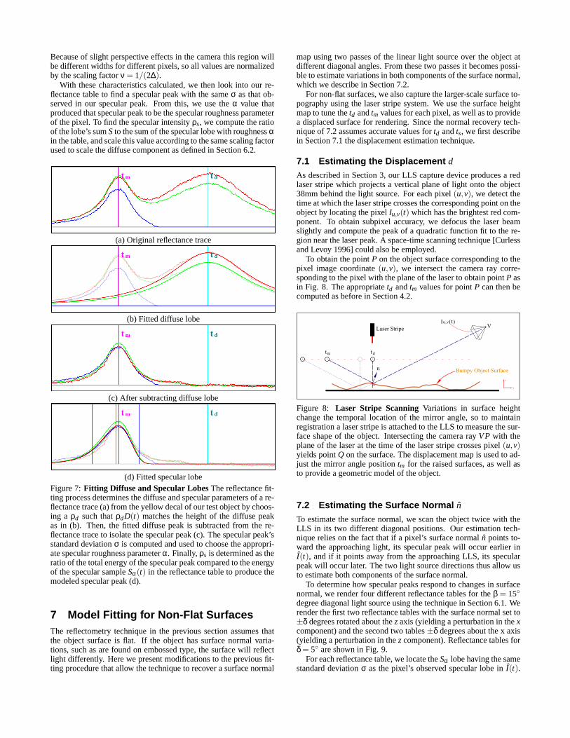
With these characteristics calculated, we then look into our re-flectance table to find a specular peak with the sameσ as that ob-served in our specular peak. From this, we use theα value thatproduced that specular peak to be the specular roughness parameterof the pixel. To find the specular intensityρs, we compute the ratioof the lobe’s sumSto the sum of the specular lobe with roughnessαin the table, and scale this value according to the same scaling factorused to scale the diffuse component as defined in Section 6.2.

(a) Original reflectance trace

(b) Fitted diffuse lobe

(c) After subtracting diffuse lobe

(d) Fitted specular lobeFigure 7:Fitting Diffuse and Specular LobesThe reflectance fit-ting process determines the diffuse and specular parameters of a re-flectance trace (a) from the yellow decal of our test object by choos-ing a ρd such thatρdD(t) matches the height of the diffuse peakas in (b). Then, the fitted diffuse peak is subtracted from the re-flectance trace to isolate the specular peak (c). The specular peak’sstandard deviationσ is computed and used to choose the appropri-ate specular roughness parameterα. Finally,ρs is determined as theratio of the total energy of the specular peak compared to the energyof the specular sampleSα(t) in the reflectance table to produce themodeled specular peak (d).

7 Model Fitting for Non-Flat SurfacesThe reflectometry technique in the previous section assumes thatthe object surface is flat. If the object has surface normal varia-tions, such as are found on embossed type, the surface will reflectlight differently. Here we present modifications to the previous fit-ting procedure that allow the technique to recover a surface normal

map using two passes of the linear light source over the object atdifferent diagonal angles. From these two passes it becomes possi-ble to estimate variations in both components of the surface normal,which we describe in Section 7.2.

For non-flat surfaces, we also capture the larger-scale surface to-pography using the laser stripe system. We use the surface heightmap to tune thetd andtm values for each pixel, as well as to providea displaced surface for rendering. Since the normal recovery tech-nique of 7.2 assumes accurate values fortd andts, we first describein Section 7.1 the displacement estimation technique.

7.1 Estimating the Displacement d

As described in Section 3, our LLS capture device produces a redlaser stripe which projects a vertical plane of light onto the object38mm behind the light source. For each pixel(u,v), we detect thetime at which the laser stripe crosses the corresponding point on theobject by locating the pixelIu,v(t) which has the brightest red com-ponent. To obtain subpixel accuracy, we defocus the laser beamslightly and compute the peak of a quadratic function fit to the re-gion near the laser peak. A space-time scanning technique [Curlessand Levoy 1996] could also be employed.

To obtain the pointP on the object surface corresponding to thepixel image coordinate(u,v), we intersect the camera ray corre-sponding to the pixel with the plane of the laser to obtain pointP asin Fig. 8. The appropriatetd andtm values for pointP can then becomputed as before in Section 4.2.

V

n

P

Bumpy Object Surface

Laser Stripe

tdtm

Iu,v(t)

y

z

Figure 8: Laser Stripe Scanning Variations in surface heightchange the temporal location of the mirror angle, so to maintainregistration a laser stripe is attached to the LLS to measure the sur-face shape of the object. Intersecting the camera rayVP with theplane of the laser at the time of the laser stripe crosses pixel(u,v)yields pointQ on the surface. The displacement map is used to ad-just the mirror angle positiontm for the raised surfaces, as well asto provide a geometric model of the object.

7.2 Estimating the Surface Normal n

To estimate the surface normal, we scan the object twice with theLLS in its two different diagonal positions. Our estimation tech-nique relies on the fact that if a pixel’s surface normal ˆn points to-ward the approaching light, its specular peak will occur earlier inI(t), and if it points away from the approaching LLS, its specularpeak will occur later. The two light source directions thus allow usto estimate both components of the surface normal.

To determine how specular peaks respond to changes in surfacenormal, we render four different reflectance tables for theβ = 15◦

degree diagonal light source using the technique in Section 6.1. Werender the first two reflectance tables with the surface normal set to±δ degrees rotated about thezaxis (yielding a perturbation in thexcomponent) and the second two tables±δ degrees about the x axis(yielding a perturbation in thezcomponent). Reflectance tables forδ = 5◦ are shown in Fig. 9.

For each reflectance table, we locate theSα lobe having the samestandard deviationσ as the pixel’s observed specular lobe inI(t).

(a) (b) (c) (d)Figure 9:Reflectance Tables for Varying Surface NormalTo an-alyze surface normal variations using the specular lobe, we renderout Sα(t) reflectance tables for theβ = 15◦ LLS angle for surfacenormals pointing slightly (a) up, (b) down, (c) left, and (d) rightfrom the light source. Perturbing the normal changes the time ofthe specular peak’s meanµ, allowing us to estimate both compo-nents of a pixel’s surface normal ˆn.

We then find the corresponding meansµx−,µx+,µz−,µz+ of each ofthese lobes. We use these four means to produce a linear functionf+15(∆x,∆z) mapping normal perturbation to mean. By symmetry,we can construct a similar functionf−15(∆x,∆z) for β =−15◦, bysimply swapping the values ofµx− andµx+. For the pixel beingconsidered, we solve for the normal perturbation components∆xand ∆z by equating f+15(∆x,∆z) and f−15(∆x,∆z) to the pixel’sactual measured means for the two LLS runs,µ+15 andµ−15. Thisyields the following 2×2 linear system:

µ+15 =µx−+µx+ +µz−+µz+

4+

∆x2δ

(µx+−µx−)+∆z2δ

(µz+−µz−)

µ−15 =µx−+µx+ +µz−+µz+

4+

∆x2δ

(µx−−µx+)+∆z2δ

(µz+−µz−)

Since this technique for computing surface normals depends onanalyzing specular reflection, it works well on specular surfacesand poorly on diffuse surfaces. For this reason, we produce our finalsurface normal map by combining the surface normals estimated byspecular reflection (Fig. 13(e) and (f), insets) with surface normalsobtained by differentiating our laser-scanned displacement mapd(Fig. 13(e) and (f)). To blend between these normal estimates, wefound good results could be obtained by using the specular-derivednormals when the ratioρs/α > 0.5, the displacement-derived nor-mals whenρs/α < 0.2, and a linear blend of the two estimates forintermediate values ofρs/α.

7.3 Adjusting for Surface Normal n

Once we have estimated a surface normal for each pixel, we canre-estimate the diffuse and specular parameters based on this im-proved knowledge of the surface characteristics. In particular, wecan adjust our model of the diffuse lobe to be rendered with thisnew surface normal. To facilitate this we pre-compute a 20× 20table of diffuse lobesD′

x,z(t) for surface normals varying inx andz, and use bilinear interpolation to create aD′(t) for the particularsurface normal. From this we re-computeρd and then produce anew specular reflectance traceI ′(t) = I(t)−D′(t). From this newreflectance trace, we fir a newSα(t) to obtain new parametersρsand α. We find that one iteration of this procedure significantlyincreases the consistency of the specular roughness parameters.

8 Estimating the Translucency ρtrans

Thin objects such as manuscripts can be translucent, which meansthat they will transmit light through the front when lit from behind.We solve for this translucency componentρtrans by taking one ad-ditional image of the objectIbacklit as illuminated from behind bythe light box, as well as an image of the light box with the objectremovedIlightbox. A set of two such images are shown in Figure 10.

(a) (b)Figure 10:Capturing the Translucent Component We measurethe translucent component of the object by taking two images withthe light box illuminated at the end of the LLS passes, one withand one without the object. Dividing the first image by the secondyields the translucency componentρtrans for each pixel and colorin Fig. 13(f).

To determine the amount of transmitted light for each pixel ofeach color channel, we computeρtrans = Ibacklit/Ilightbox to obtainthe percent of light transmitted at each pixel. In our reflectancemodel, we assume that any light transmitted through the materialbecomes diffused, so we do not measureρtrans for different incidentand outgoing directions. This is a simplified model of translucencyin comparison to subsurface scattering methods as in [Jensen et al.2001], but we have found it to approximate the scattering charac-teristics of our test object sufficiently.

9 ResultsIn this section we present the recovered reflectance parameters fortwo objects and renderings of the captured models under variouslighting conditions. Our renderer was created by implementing theWard model as a floating-point pixel shader in Direct X 9 on anATI Radeon 9700 graphics card, allowing all surface maps and ren-dered values to be computed radiometrically linearly in high dy-namic range. Our first object seen in Fig. 11 was chosen to test thealgorithm’s ability to capture varying diffuse and specular proper-ties for the flat object case. It consists of an 8.5× 11 inch shinyblack card printed with black laser toner, which provides a dullspecularity. Attached are four glossy color decals, and we placedan oily thumbprint in the center of the shiny black area. Since therewere no significant variations in surface normal, we scanned theobject with a single pass of the LLS to obtain its spatially-varyingreflectance parametersρd,ρs,α shown in 11.

For validation, we found that the recoveredρd parameters prop-erly ranged between 0 and 1 and were consistent with measure-ments taken with a calibrated spectroradiometer. We also generatedrenderings of the surface under point-light source illumination inour interactive renderer as in 12(b) which are largely consistent withthe actual appearance of the object. One noticeable difference is thegreater breadth of the real specular lobe in the shiny black material,which we believe to be an artifact of the Ward reflectance modelnot precisely matching the toe behavior of this particular specu-lar material, even if the overall height and width of the lobe areconsistent. This result suggests that investigating fitting to moreelaborate reflectance models could be useful. Also apparent is abright rim of light on the upper right of the inner circle not presentin the real image. We determined that this behavior resulted whenfitting the behaviors of pixels which cover a heterogenous area ofboth sharp and dull specular material - the fitted peak produces abroader lobe than the sharp specularity and a higher reflectance inthe off-specular region, yielding reflected light in the off-specularregion not exhibited by the heterogenous material. This result sug-gests that investigating fitting mixed specular models in regions ofhigh specular variance.

For our second example we captured the reflectance properties of

(a) Diffuse Colorρd (b) Specular Intensityρs (c) Specular Roughnessα

Figure 11:Recovered Reflectance Parameters for the Test Object

(a) (b)Figure 12:Real and Synthetic Comparison (a)Real photographof test object.(b) Real-time rendering of the captured reflectanceproperties of the test object.

a 177×163mm page from a 15th-century illuminated manuscriptseen in Fig. 14(a). The manuscript is written on vellum animal-skin parchment and features several embossed gold ”illuminated”letters, which tested our method’s ability to capture metallic spec-ularity, surface normal variation, and translucency. Since themanuscript did not lie flat on the light box, it also exercised ourtechnique’s ability to capture and compensate for varying surfacedisplacement. We captured two passes of the LLS at±15◦ at 0.9mm intervals. The manuscript’s recoveredρd,ρs,α,d,n, andρtransparameters are shown in 13.

The algorithm found that the manuscript’s vellum surface exhib-ited a dull specularity, and as expected found that the gold lettershad a greater specular intensity and lower roughness than the vel-lum. Theρtrans values indicated that the manuscript transmits ap-proximately 17% of the red light, 14% of the green light, and 9% ofthe blue light. Renderings produced of the manuscript under vari-ous point light directions as in Fig. 14 were largely consistent withthe actual appearance of the manuscript under similar lighting con-ditions. For some angles our modeled manuscript appeared to beslightly more specular than the original; a possible explanation isthat the vellum exhibits a forward-scattering component which ismistaken as additional specularity by our lighting capture system.To test our surface normal recovery, we compared the appearanceof the illuminated letter ”D” in for real and synthetic images (Fig.15). We found the normals to be largely consistent though the re-

(a) (b)Figure 14: Real and Synthetic Comparison (a)Real photo-graph of the manuscript.(b) Real-time rendering of the modeledreflectance properties of the manuscript lit from a similar direction.

flections had less texture and were somewhat duller; these resultssuggest that using a narrower LLS might improve the results forsharp specular surfaces. The video accompanying this paper showsreal and synthetic animation of the manuscript under point lightsource illumination.

To show a lighting configuration that would exhibit both themanuscript’s reflective and translucent qualities, we implementeda multipass renderer to illuminate our manuscript with an omnidi-rectional lighting environment acquired inside a cathedral. Resultsof rendering both the manuscript and the test object in this lightingenvironment are shown in Fig. 16.

10 Discussion and Future WorkThe capabilities and limitations of our linear light source reflectom-etry system suggest several avenues of work for future versions ofthe system.

In this work we recover trichromatic measurements of the ob-ject’s diffuse, specular, and transmissive reflectance properties, ow-ing to the fact that we use a standard RGB digital camera. Such anapproximation to a description of the full spectral reflectance cancause errors in rendering the object under novel lighting conditions[Borges 1991]. This is a concern since a common application of

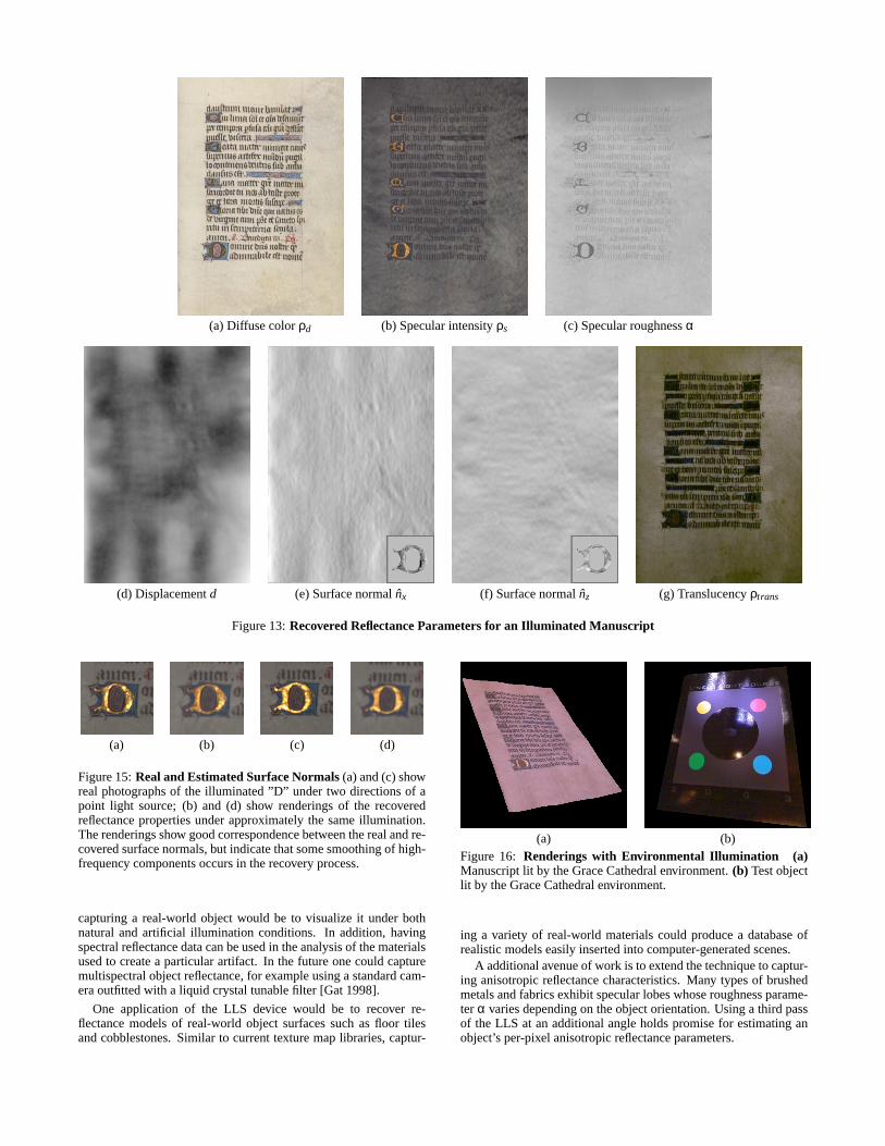
(a) Diffuse colorρd (b) Specular intensityρs (c) Specular roughnessα

(d) Displacementd (e) Surface normal ˆnx (f) Surface normal ˆnz (g) Translucencyρtrans

Figure 13:Recovered Reflectance Parameters for an Illuminated Manuscript

(a) (b) (c) (d)

Figure 15:Real and Estimated Surface Normals(a) and (c) showreal photographs of the illuminated ”D” under two directions of apoint light source; (b) and (d) show renderings of the recoveredreflectance properties under approximately the same illumination.The renderings show good correspondence between the real and re-covered surface normals, but indicate that some smoothing of high-frequency components occurs in the recovery process.

capturing a real-world object would be to visualize it under bothnatural and artificial illumination conditions. In addition, havingspectral reflectance data can be used in the analysis of the materialsused to create a particular artifact. In the future one could capturemultispectral object reflectance, for example using a standard cam-era outfitted with a liquid crystal tunable filter [Gat 1998].

One application of the LLS device would be to recover re-flectance models of real-world object surfaces such as floor tilesand cobblestones. Similar to current texture map libraries, captur-

(a) (b)Figure 16: Renderings with Environmental Illumination (a)Manuscript lit by the Grace Cathedral environment.(b) Test objectlit by the Grace Cathedral environment.

ing a variety of real-world materials could produce a database ofrealistic models easily inserted into computer-generated scenes.

A additional avenue of work is to extend the technique to captur-ing anisotropic reflectance characteristics. Many types of brushedmetals and fabrics exhibit specular lobes whose roughness parame-ter α varies depending on the object orientation. Using a third passof the LLS at an additional angle holds promise for estimating anobject’s per-pixel anisotropic reflectance parameters.

Finally, the design of our current LLS apparatus limits its appli-cation to relatively flat objects such as printed materials and fabrics.It would be desirable to extend these techniques to be able to cap-ture the spatially varying reflectance characteristics of completely3D objects such as human faces and painted sculptures. By improv-ing the laser scanning system and assembling multiple LLS scansof an object from different angles, it could be possible to create 3Dmodels of real-world objects which faithfully reproduce the object’sreflectance properties.

11 ConclusionIn this paper we have presented a system for capturing the spa-tially varying diffuse and specular reflectance properties real-worldobject surfaces using a linear light source, and have applied ourtechnique to a test object and an illuminated manuscript. The ap-paratus can be built at low cost, requires modest scanning time andcomputation, and produces realistic and largely faithful models ofthe real object’s reflectance characteristics. Augmented by someof the techniques proposed as future work, this form of object cap-ture could become a useful tool for computer graphics practitionerswanting to capture the realism of real-world reflectance properties,as well as to museum conservators and researchers wishing to digi-tally preserve, analyze, and communicate cultural artifacts.

AcknowledgementsWe gratefully acknowledge Mark Brownlow for helping constructthe LLS apparatus and the test sample, Brian Emerson for videoediting, Maya Martinez for finding reflectance samples, AndreasWenger for designing the motion-control system for photograph-ing the real/synthetic comparisons, Jessi Stumpfel for producingreflectance graphs, Donat-Pierre Luigi for camera calibration andbackground research, and Diane Piepol for producing the projectand Karen Dukes for providing assistance. We especially thankAlexander and Judy Singer for providing manuscript reproductionsfor testing the apparatus, Martin Gundersen and Charles Knowltonfor helpful light source discussions, Greg Ward for helpful reflec-tometry discussions, and Richard Lindheim, Neil Sullivan, JamesBlake, and Mike Macedonia for supporting this project. This workhas been sponsored by U.S. Army contract number DAAD19-99-D-0046 and the University of Southern California; the content ofthis information does not necessarily reflect the position or policyof the sponsors and no official endorsement should be inferred.

ReferencesBORGES, C. F. 1991. Trichromatic approximation for computer graphics illumination

models. InComputer Graphics (Proceedings of SIGGRAPH 91), vol. 25, 101–104.

CHUANG, Y.-Y., ZONGKER, D. E., HINDORFF, J., CURLESS, B., SALESIN, D. H.,AND SZELISKI , R. 2000. Environment matting extensions: Towards higher accu-racy and real-time capture. InProceedings of SIGGRAPH 2000, 121–130.

COOK, R. L., AND TORRANCE, K. E. 1981. A reflectance model for computer graph-ics. Computer Graphics (Proceedings of SIGGRAPH 81) 15, 3 (August), 307–316.

CURLESS, B., AND LEVOY, M. 1996. Better optical triangulation through spacetimeanalysis. InProceedings of SIGGRAPH 95, International Conference on ComputerVision, 987–994.

DANA , K. J., GINNEKEN, B., NAYAR , S. K., AND KOENDERINK, J. J. 1997. Re-flectance and texture of real-world surfaces. InProc. IEEE Conf. on Comp. Visionand Patt. Recog., 151–157.

DEBEVEC, P. E., AND MALIK , J. 1997. Recovering high dynamic range radiancemaps from photographs. InSIGGRAPH 97, 369–378.

DEBEVEC, P. E., TAYLOR , C. J., AND MALIK , J. 1996. Modeling and renderingarchitecture from photographs: A hybrid geometry- and image-based approach. InSIGGRAPH 96, 11–20.

DEBEVEC, P., HAWKINS , T., TCHOU, C., DUIKER, H.-P., SAROKIN , W., AND

SAGAR, M. 2000. Acquiring the reflectance field of a human face.Proceedings ofSIGGRAPH 2000(July), 145–156.

GAT, N. 1998. Real-time multi- and hyper-spectral imaging for remote sensing andmachine vision: an overview. InProc. 1998 ASAE Annual International Mtg.

HALSTEAD, M., BARSKY, B. A., KLEIN , S.,AND MANDELL , R. 1996. Reconstruct-ing curved surfaces from specular reflection patterns using spline surface fitting ofnormals. InProceedings of SIGGRAPH 96, Computer Graphics Proceedings, An-nual Conference Series, 335–342.

HANRAHAN , P., AND KRUEGER, W. 1993. Reflection from layered surfaces due tosubsurface scattering.Proceedings of SIGGRAPH 93(August), 165–174.

JENSEN, H. W., MARSCHNER, S. R., LEVOY, M., AND HANRAHAN , P. 2001. Apractical model for subsurface light transport. InProceedings of SIGGRAPH 2001,ACM Press / ACM SIGGRAPH, Computer Graphics Proceedings, Annual Confer-ence Series, 511–518. ISBN 1-58113-292-1.

LAFORTUNE, E. P. F., FOO, S.-C., TORRANCE, K. E., AND GREENBERG, D. P.1997. Non-linear approximation of reflectance functions.Proceedings of SIG-GRAPH 97, 117–126.

LARSON, G. J. W. 1992. Measuring and modeling anisotropic reflection. InComputerGraphics (Proceedings of SIGGRAPH 92), vol. 26, 265–272.

LENSCH, H. P. A., KAUTZ , J., GOESELE, M., HEIDRICH, W., AND SEIDEL, H.-P. 2001. Image-based reconstruction of spatially varying materials. InRenderingTechniques 2001: 12th Eurographics Workshop on Rendering, 103–114.

LEVOY, M., PULLI , K., CURLESS, B., RUSINKIEWICZ, S., KOLLER, D., PEREIRA,L., GINZTON, M., ANDERSON, S., DAVIS , J., GINSBERG, J., SHADE, J., AND

FULK , D. 2000. The digital michelangelo project: 3d scanning of large statues.Proceedings of SIGGRAPH 2000(July), 131–144.

MALZBENDER, T., GELB, D., AND WOLTERS, H. 2001. Polynomial texture maps.Proceedings of SIGGRAPH 2001(August), 519–528.

MARSCHNER, S. R., WESTIN, S. H., LAFORTUNE, E. P. F., TORRANCE, K. E.,AND GREENBERG, D. P. 1999. Image-based BRDF measurement including hu-man skin.Eurographics Rendering Workshop 1999(June).

MARSCHNER, S. 1998.Inverse Rendering for Computer Graphics. PhD thesis, Cor-nell University.

MCALLISTER, D. K. 2002. A Generalized Surface Appearance Representation forComputer Graphics. PhD thesis, University of North Carolina at Chapel Hill.

NAYAR , S. K., IKEUCHI, K., AND KANADE , T. 1994. Determining shape andreflectance of hybrid surfaces by photometric sampling.IEEE Transactions onRobotics and Automation 6, 4 (August), 418–431.

NICODEMUS, F. E., RICHMOND, J. C., HSIA, J. J., GINSBERG, I. W., AND

L IMPERIS, T. 1977. Geometric considerations and nomenclature for reflectance.National Bureau of Standards Monograph 160(October).

NISHITA , T., OKAMURA , I., AND NAKAMAE , E. 1985. Shading models for pointand linear sources.ACM Transactions on Graphics 4, 2 (April), 124–146.

OREN, M., AND NAYAR , S. K. 1994. Generalization of Lambert’s reflectance model.Proceedings of SIGGRAPH 94(July), 239–246.

POULIN , P., AND AMANATIDES , J. 1991. Shading and shadowing with linear lightsources.Computers & Graphics 15, 2, 259–265.

POULIN , P., AND FOURNIER, A. 1990. A model for anisotropic reflection. InCom-puter Graphics (Proceedings of SIGGRAPH 90), vol. 24, 273–282.

RAMAMOORTHI , R., AND HANRAHAN , P. 2001. A signal-processing framework forinverse rendering. InProceedings of ACM SIGGRAPH 2001, ACM Press / ACMSIGGRAPH, Computer Graphics Proceedings, Annual Conference Series, 117–128. ISBN 1-58113-292-1.

RUSHMEIER, H., BERNARDINI, F., MITTLEMAN , J., AND TAUBIN , G. 1998. Ac-quiring input for rendering at appropriate levels of detail: Digitizing a pieta. Euro-graphics Rendering Workshop 1998(June), 81–92.

SATO, Y., WHEELER, M. D., AND IKEUCHI, K. 1997. Object shape and reflectancemodeling from observation. InSIGGRAPH 97, 379–387.

TORRANCE, K. E., AND SPARROW, E. M. 1967. Theory for off-specular reflectionfrom roughened surfaces.Journal of Optical Society of America 57, 9.

WARD, G. J. 1992. Measuring and modeling anisotropic reflection. InSIGGRAPH92, 265–272.

YU, Y., DEBEVEC, P., MALIK , J.,AND HAWKINS , T. 1999. Inverse global illumina-tion: Recovering reflectance models of real scenes from photographs.Proceedingsof SIGGRAPH 99(August), 215–224.

ZONGKER, D. E., WERNER, D. M., CURLESS, B., AND SALESIN, D. H. 1999.Environment matting and compositing.Proceedings of SIGGRAPH 99(August),205–214.