Numerical solutions of systems of linear equations1

V. B. Yap2, Q. Sheng3

1. Introduction

A vector is a collection of items. A set of vectors with certain proper­ties, such as with the same number of items, forms a vector space. Rn is the vector space wherein the vectors have n real items each. If the items are complex numbers, en is used to denote the vector space. Rn c en, I.e., Rn is a subspace of en. For x,y E en, define z =X± y as

z= [

X1 ± Y1 l XnlYn

or z, = x, ± Yi, i = 1, ... , n

and z E en. A matrix is a rectangular array of numbers. Let A be a matrix of size

n x m, i.e., n rows by m columns, then

a~m ] or [a,; ]i=1,2, ... ,n; ;=1,2, ... ,m

anm

where i and j are known as the row and column number respectively. For a square matrix of size n X n, au, a22 , ••• ,ann are known as the diagonal entries. Rnxn is1 the matric space containing n X n matrices with real numbers and enxn, complex numbers. For A, B E enxn, define P = A+ B and Q = AB as

p = [ au 7 bu

an1 + bn1

a1n + b1n l : or Pi; = a,; + b,,;,

ann~ bnn

i,j=1,2, ... ,n,

1 Paper presented to the Science Research Congress 1991 as part of the 1991 SRP organised jointly by the National University of Singapore and the Ministry of Education.

2Raffies Junior College, Mount Sinai Road, Singapore 1027. 3Department of Mathematics, National University of Singapore, Kent Ridge, Singapore 05U.

18

r

n

or Qii = L 0-i~cb~e;, lc=l

i,j=1, ... ,n,

and P, Q E cnxn. Generally AB =/= BA. For other matrices, AB is defined if and only if the number of columns of A equals that of rows of B. A square matrix A is singular if and only if IAI = 0. A vector is a special matrix with size n x 1.

Consider the system of linear equations

where aii and bi are real constants and Xi are unknowns (i,j = 1, 2, ... , n). The above linear system can be written in an equivalent matrix form:

Ax= b, A E Rnxn, x,b ERn,

where

Systems of linear equations have a wide range of applications in both theoritical and practical sciences. Our study attempts to give a brief in­troduction to the numerical solutions of the linear systems together with some important theorems in linear algebra. Several algorithms for solving linear systems are developed using Fortran 77. Partial pivoting is intro­duced to achieve accuracy and applicability. L U decomposition is studied and the operation count for Gaussian elimination is given and compared to other methods. The programs are then tested with an ill-conditioned system and a nuclear reactor problem. Errors in the discretizations are estimated.

19

2. Analysis and Algorithms

(a) Preliminary and Analysis Let A be ann X m matrix. The transpose of A, denoted AT, is obtained

by making the ith row of A the ith column of AT and is given by

The conjugate transpose of A, denoted A*, is obtained in a similar way and is given by

* -ai; = a;i·

Thus AT and A* are m x n matrices. We may prove

Lemma 2.1. For A, B E cnxn (a) A+B = B+A, (b) (A+B)+C = A+(B+C), (c) A(B+C) =

AB+AC; (d) A(BC) = (AB)C, (e) (A+B)T =AT +BT, (f) (AB)T = BT AT.

A is called symmetric if AT= A, and Hermitian if A* =A. The term symmetric is generally used only with real matrices. Let A be a Hermitian matrix. It is called positive definite if and only if XT Ax > 0, Vx E en' X t­o = [0, 0, ... 'o]T. Positive definite matrices possess important properties and occur in a wide variety of applications.

A norm of a vector x is a function f : Rn ~---+ R which gives the size of the vector and is denoted by llxll· A useful class of norms are the Holder or p-norms defined by

1

llxllp = (jx1jP + · · · + lxniP)P P ~ 1.

Of which llxll 17 1!xll2 and llxlloo are the most important. Similar norms can be defined for matrices. We have

Theorem 2.1. If A E Rnxn, the following statements are equivalent. (a) A= MMT with ME Rnxn and jMj f. 0. (b) A is positive definite. (c) There exists a lower triangular matrix L with L E Rnxn such that

A= LLT.

111 0 0

L=

20

.. I

Proof. Let M = {mi;},A = {ai;}, i,;' = 1,2, ... ,n. Then MT = {m;i}·

n n

ai; = 2:::::: mu,mf; = 2:::::: mi~cm;~c, k=1 k=1

n n

a;i = 2:::::: m;~cmf. = 2:::::: m;~cmik· k=1 k=1

Therefore A is symmetric. Furthermore, we have

= (MTxfMTx

= IIMT xll~ > 0, X ERn, X=/= 0 .

Therefore A is positive definite. 0

Corollary 2.1. If A E cnxn is positive definite, then ai; > 0 for i 1,2, ... ,n. {b) Algorithm I: Gaussian Elimination

Consider a real linear system

Ax= b, A E Rnxn, x,b ERn, IAI =I= 0.

We wish to reduce A to an upper triangular matrix which is easier to solve. The process of reducing A and subsequently solving for xis known as Gaussian elimination. Denote A by A (1), we have

Step 1: Assuming aW =/= 0, for i = 1, 2, ... , n, define row multipliers

and define (2) - (1) (1) . ai; - ai; - mila1; , J = 2, 3, ... , n,

21

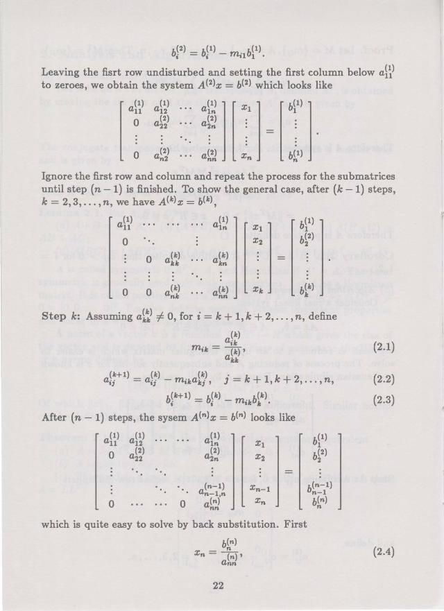
b(2) - b(1) - . b(1) i - i m,1 1 •

Leaving the fisrt row undisturbed and setting the first column below aW to zeroes, we obtain the system A<2>x = b(2) which looks like

(1) au 0

0

Ignore the first row and column and repeat the process for the submatrices until step (n -1) is finished. To show the general case, after (k -1) steps, k = 2, 3, ... , n, we have A (k) x = b(k),

(1) au

(1) aln

0

0 (k) akk

(k) akn

0 0 (k) a(k) ank nn

Step k: Assuming a~~ =/= 0, for i = k + 1, k + 2, ... , n, define

(k) _ aik

m;k- W' akk

(k+l) (k) (k) . k k a;; = a;; - m;kak; , J = + 1, + 2, ... , n,

b(k+1) - b(k) - . b(k) i - i m,k k •

After (n- 1) steps, the sysem A(n),x = b(n) looks like

(1) (1) ... . . . (1) au a12 a1n X1

0 (2) (2) a22 a2n .x2

(n-1) Xn-1 an-1,n

0 0 a(n) Xn nn

which is quite easy to solve by back substitution. First

b(n) n xn=w,

ann

22

b~1)

b~2)

b(n-1) n-1 b(n) n

(2.1)

(2.2)

(2.3)

(2.4)

then

k = n- 1, n- 2, ... , 1. (2.5)

This completes the algorithm. Equations (2.1) to (2.5) are used to write a Fortran program (Program 1) which performs the Gaussian elim­ination. It is to be noted that Gaussian elimination algorithms are not unique. There are other ways to reduce A to an upper triangular or even a lower triangular matrix. In that case, forward substitution is used. Re­gardless of the different methods used, the solutions should be identical theoritically. However, from the point of view of numerical analysis, dif­ferent computers and programs may give different answers for the same problem. We will see this in the next section.

(c) Algorithm II: L U Decomposition Construct the matrices L and U where

1 0 0 uu ul2 ... . . . U1n

m21 1 0 U22

L= U= = A(n).

1 o· Un-1,n

mn1 ... . . . mn,n-1 1 0 0 Unn

This is called the LU decomposition of A which is very useful as Land U can be stored together as a matrix(ignoring the diagonal entries of L) in the computer. If A appears in other systems, then we need only to modify b using the row multipliers to obtain the solution.

Lemma 2.2. A = LU and IAI = uuu22 ••• Unn·

Proof. For j 2: i,

[ mib ... , mi.i-b 1, 0, ... , 0 ] uii 0

0

23

i-1

= L m,"u"i + uii k=1

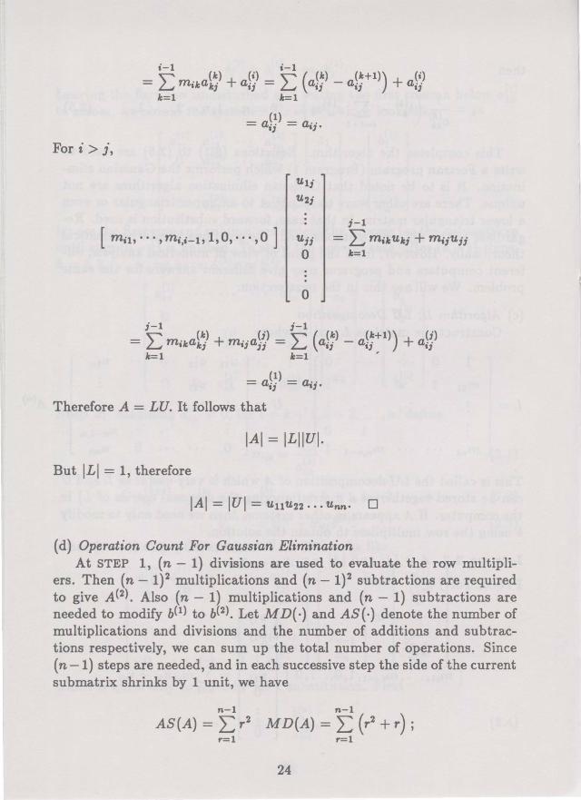
i-1 i-1

= "\""' m,·~calc(~) +a(') = "\""' (a(~) - a(~+l)) + a(') LJ J IJ LJ IJ IJ IJ lc=1 lc=1

- a(t)- a·· - ij - .,.

Fori> j,

[ m,h · · ·, mi,i-1! 1, 0, · · ·, 0 ] u;;

0

j-1

= L m,~cu~c; + m,;u;; lc=1

0

j-1 j-1

= L m,~ca~~) + m,;aW = L (a~;)- a~;+l)) + aW lc=1 lc=l ,

= a~J) =a.;.

Therefore A = LU. It follows that

IAI=ILIIUI.

But ILl = 1, therefore

IAI = lUI = 'UntL22 • • • 'Unn• D

(d) Operation Count For Gaussian Elimination At STEP 1, (n- 1) divisions are used to evaluate the row multipli­

ers. Then (n- 1)2 multiplications and (n- 1)2 subtractions are required to give A(2). Also (n- 1) multiplications and (n- 1) subtractions are needed to modify b(1) to b(2). Let MD(·) and AS(·) denote the number of multiplications and divisions and the number of additions and subtrac­tions respectively, we can sum up the total number of operations. Since ( n -1) steps are needed, and in each successive step the side of the current submatrix shrinks by 1 unit, we have

n-1 n-1

AS(A) = L r 2 MD(A) = L (r2 + r); r=1 r=1

24

n-1 n-1 AS(b) = L r MD(b) = L r;

r=1 r=1 n-1 n-1 2n3 - 2n n3

AS(A) + AS(b) = L r2 + L r =

6 ~ 3'

r=1 r=1 n-1 n-1 2n3 + 3n2 - 5n ns

MD(A)+MD(b)=L:r 2 +2L:r= 6

~3. r=1 r=1

The number of additions is almost the same to that of multiplications and divisions, so we consider only the latter. Gaussian elimination is less troublesome than multiplying two n x n matrices which requires n3

operation. It is also better than the Cramer's rule by which the operation count is (n + 1)! if the determinants are computed using expansion by minors or the Gauss-Jordan method which requires ln3 operations.

(e) Algorithm III: Partial Pivoting In the algorithm, we assume that the pivot element a~~ f= 0, k

1, 2, ... , n. This assumption can be removed by switching the rows such that the pivot element is always nonzero. But in computer operations, a zero may not be exactly zero due to errors, and if we happen to make this 'nonzero' the pivot, gross error will result. Partial pivoting is a technique designed to avert this danger.

Define Si = m?JC la~!)l, k = 1,2, ... ,n.

k$t$n

If Si f= Ia~~ I, interchange the ith row and the kth row in A and B and it is certain that the pivot element will not be zero, for if a~!) = 0, IAI = 0, contrary to the condition of A. Note that by doing so, lmik ~ 11 for i = k+ 1, k + 2, ... , n, and this will prevent the elements from being magnified in subsequent elimination which will cause severe loss of significant figures in the floating point representation of numbers in the computer. In Program 2, partial pivoting is used.

3. Applications

(a) An fll-conditioned {Stiff) Problem Given the system

6x1 + 2x2 + 2xs = -2; 2 1

2x1 + 3x2 + 3xs = 1;

25

X1 + 2x2 - X3 = 0.

Solving without partial pivoting using Program 1, the solution,

x 1 = -3.97682137 X 107, x2 = 1.19304647 X 108

, x3 = -5.00000000,

is disastrous. But with partial pivoting (Program 2), the approximately correct solution is found:

X1 = 2.60000006, X2 = -3.79999990, Xs = -4.99999988.

Using another version of the Gaussian elimination (Program 3) without partial pivoting, we get the wrong answers:

X 1 = 1.33333333, x 2 = 0.00000000, x 3 = -5.00000000.

With partial pivoting, the solution is even closer to the true one:

X 1 = 2.60000006, X2 = -3.80000000, Xs = -5.00000000.

This type of problem is called ill-conditioned or stiff. The slight differ­ence in the two correct solutions is due to comput~r round-off error. It is stressed that by doing hand calculations, we get the exact solution with or without partial pivoting.

(b) A Nuclear Reactor Problem In a unit square area n of a nuclear reactor, the pressure function U

satisfies the partial differential equation

flU- aU= 0

where a2 a2 ll = ax2 + ay2 and a= sin

3 (x + y),

with boundary functions given as follows: A : u = p = (1- y) 2y2

' if X= 0, 0 ::; y ::; 1; B : U = Q = sin3 411"x, if 0 ::; x ::; 1, y = 1; C : U = R = xy ( 1 - y), if x = 1, 0 ::; y ::; 1;

(3.1)

D : U = S = sin 211"x, if 0 ::; x ::; 1, y = 0. We wish to find the numerical values of U for points in n. Let N ~ 1(N E Z+), define

h= 1 N + 1'

(3.2)

26

(x;, Yk) = (jh, kh) E 0, j, k = 1, 2, ... , N.

These are called grid points or mesh points and they are labelled in the order shown in the sketch. Let the value of U at point n ( n = 1, 2, ... , N 2 ) be Un. We approximate equation (3.1) by means of the fi­nite difference method. Using central differences, we have

8 2U ,.._ u A- U(x + h,y)- 2U(x,y) + U(x- h,y) 8x2 - zz- h2

82U ,.._ UAA - U(x, y +h) - 2U(x, y) + U(x, y- h) 8y2 - 1111- h2

Substituting the above expressions into (3.1), we get the difference equa­tion

U(x+ h, y) + U(x- h,y) + U(x, y+h) + U(x,y- h)- (4 +ah2 )U(x, y) = 0. (3.3)

For the point (x;, Yk) E 0, from equation (3.3),

U(x;+b Yk)+U(x;-b YA:)+U(x;, Yk+I)+U(x;, Yk-1)-(4+ah2)U(x;, Yk) = 0. (3.4)

This will be used to find the equation on each grid point. For example, at point 1, j = k = 1, equation (3.4) becomes

which gives

U2 + P(O, h)+ UN+l + S(h, 0) - (4 + ah2 )U1 = 0.

Bringing the constants to the right, we obtain the first linear equation. Similarly for the remaining grid points. Arranging the N 2 equations in N 2

unknowns into a system according to the order of grid points, we can solve it using Gaussian elimination. Let us call the system AU = b. A data file is built using Program 4 to generate the entries of A, then Program 1 or 2 is used to solve the system and the numerical solutions are satisfactory.

We observed that the matrix A has several interesting properties: (a) A is called sparse because most of its elements are zeroes. (b) Nonzeroes can only be found in five diagonal lines, so A is called a

band matrix. (c) It is called block tridiagonal because if A were partitioned into N 2

N x N matrices, most nonzeroes will be found in blocks along the three main diagonal lines.

27

(d) It is symmetric and positive definite and by lemma 2.4, a lower triangular matrix E exists such that A = E ET.

(e) It is diagonally dominant, meaning the absolute values of the di­agonal elements are numerically larger than others in their correponding rows and columns.

(f) The matrices L and U obtained by LU decomposition are also sparse.

This type of matrix has important applications in solving many prac­tical problems.

(c) Truncation Error In The Discretization Using Taylor's expansion, we know that the error in Uu,,

2h2 a4U 2h2"-2 a2"U =--+···+ --+··· 4! ax4 (2n)! ax2" •

Similarly error in U00 ,

2h2 a4U 2h2"-2 a2"U err II = -, -a 4 + • • • + ( ) I a 2n + .... 4. y 2n. y

Define

Total error

00 h2k-2 = 2 2: -( k)' ll2"u.

k=2 2 .

As N becomes larger, h becomes smaller from equation (1), and the approximation becomes more accurate.

References

1. Kahaner, D.; Moler, C. & Nash, S. (1989): Numerical Methods and Software, Prentice-Hall International Editions.

28

2. Golub, G. H. (1983): Matrix Computations. The Johns Hopkins University Press.

3. Balfour, A. & Marwick D. H. (1983): Programming in Standard Fortran 77, Heinemann Educational Books.

4. Sheng, Q. (1989): "Solving Linear Partial Differential Equation by Exponential Splitting", IMA J. of Numerical Analysis, 9, pp 199-212.

5. Sheng, Q. (1991): Lecture Notes for Numerical Analysis. NUS.

29