Embed Size (px)
Citation preview

Linear and Kernel Classification: When to Use Which?
Hsin-Yuan Huang⇤ Chih-Jen Lin†
Abstract
Kernel methods are known to be a state-of-the-art classifi-cation technique. Nevertheless, the training and predictioncost is expensive for large data. On the other hand, linearclassifiers can easily scale up, but are inferior to kernel clas-sifiers in terms of predictability. Recent research has shownthat for some data sets (e.g., document data), linear is asgood as kernel classifiers. In such cases, the training of akernel classifier is a waste of both time and memory. Inthis work, we investigate the important issue of e�cientlyand automatically deciding whether kernel classifiers per-form strictly better than linear for a given data set. Ourproposed method is based on cheaply constructing a clas-sifier that exhibits nonlinearity and can be automaticallytrained. Then we make a decision by comparing the perfor-mance of our constructed classifier with the linear classifier.We propose two methods: the first one trains the degree-2 feature expansion by a linear-classification method, whilethe second dissects the feature space into several regions andtrains a linear classifier for each region. The design consider-ations of our methods are very di↵erent from past works forspeeding up the kernel training. They still aim at obtainingaccuracy close to the kernel classifier, but ours would like togive a quick and accurate decision without worrying aboutaccuracy. Empirically our methods can e�ciently make cor-rect indications for a wide variety of data sets. Our proposedprocess can thus be a useful component for automatic ma-chine learning.
1 Introduction
Machine learning is now widely applied in many ar-
eas, but its practical use remains challenging for non-
experts. To make machine learning an easy-to-use tech-
nique, recently automatic machine learning (autoML)
has become an important research topic. What makes
autoML a challenging task is that there are too many
considerations, and di↵erent components often inter-
twined with each other. In this work we consider the
issue of automatically choosing between linear and ker-
nel classifiers. This issue is useful in an autoML process
because very often we start with using a linear classifier
⇤Department of Computer Science, National Taiwan Univer-sity. [email protected]
†Department of Computer Science, National Taiwan Univer-sity. [email protected]
and move to a nonlinear one if the performance is not
satisfactory.
In machine learning, kernel classifiers such as sup-
port vector machines (SVM) [4] or kernel logistic regres-
sion (LR) are known to achieve state-of-the art perfor-
mances for many classification problems; see detailed
comparisons in, for example, [18, 6]. However, training
and prediction are slow because kernel methods nonlin-
early map data to a high dimensional space and employ
the kernel trick. In contrast, linear classifiers of work-
ing in the original feature space are much more scalable.
Although classifiers employing certain kernels are the-
oretically known to be at least as good as linear [12],
1
for many problems (e.g., document classification) linear
classifiers are known to be competitive (e.g., the survey
in [25]). For such data, the training of kernel classifiers
is a total waste because fast and simple linear classifiers
are enough.
From the above discussion, a possible component in
an autoML workflow can be as follows.
If linear is as good as kernel, then
use a linear classifier,
else
use a kernel classifier.
Note that by kernel classification we mean that highly
nonlinear kernels are used. In fact, the most commonly
used Gaussian (RBF) kernel will be the focus in this
paper. While the above workflow is simple, the following
challenging issues must be solved first.
1. The method to check if linear classifiers are as
good as nonlinear ones must be fast, automatic, and
e↵ective. First, the procedure must be much faster than
training kernel classifiers and, if possible, as e�cient
as training linear classifiers; otherwise, the workflow
becomes useless. Second, it should not involve the
tuning of many parameters, so the use is convenient.
Third, the procedure should accurately reveal if there
is a clear performance gap between linear and kernel
classifiers.
2. Before employing a method to predict if linear is as
good as kernel, we should ensure that the linear classifier
1Specifically, [12] proves that if the Gaussian kernel is usedwith suitable kernel/regularization parameters, then the perfor-mance is at least as good as using linear.
is “under the best settings” including suitable data pre-
processing and parameter selection. Although recent
works such as [3] have made progress on this aspect,
some issues remain to be addressed.
The di�culty in di↵erentiating linear and kernel
can also be seen from our development of two popular
packages LIBSVM [1] and LIBLINEAR [5] for kernel
and linear classification, respectively. Many users have
asked why the two packages are not combined together.
However, the merge is not possible unless we have
resolved the above-mentioned issues.
In this paper, we focus on the issue of checking
if for the same data a linear classifier is as good as a
kernel one. Currently some rough guidelines are used
in practice. For example, it is mentioned in [11] that
“If the number of features is large, one may not need
to map data to a higher dimensional space.” To the
best of our knowledge, we are the first to systematically
investigate this kernel-check problem.
A well-studied topic related to our work is kernel
approximation. To reduce the lengthy running time of
training a classifier, many works [23, 26] have attempted
to approximate the kernel matrix or the kernel function.
Their goal is to make the performance close to that
of the original one, but require less time. Therefore,
both training time and performances are concerns. Ours
di↵ers from them because accuracy is not important.
It is su�cient if our method can e↵ectively tell if
kernel and linear yield di↵erent accuracy values. More
discussion is in Section 3.
This paper is organised as follows. Section 2 briefly
introduces linear and kernel classifiers, and their rela-
tions. In Section 3, we propose some e↵ective meth-
ods to check if kernels should be used. Section 4 ad-
dresses the second challenge mentioned above. We
mainly investigate some data scaling issues so that a
good setting for linear classification can be automat-
ically found. Detailed experiments are in Section 5,
while conclusions are in Section 6. Supplementary ma-
terials are at http://www.csie.ntu.edu.tw/
~
cjlin/
papers/kernel-check/supplement.pdf.
2 Linear and Kernel Classifiers
Before proposing methods to check if kernels are needed,
we check how linear and kernel classifiers are practically
used. We focus on two-class problems with training data
(yi,xi), i = 1, . . . , l, where label yi = ±1 and xi 2 Rn.
2.1 Standard Settings for Linear Classifiers A
linear classifier involves an optimization problem.
(2.1) min
w
1
2
w
Tw + C
Xl
i=1⇠(w; yi,xi),
where C is the regularization parameter and ⇠(w; y,x)
is the loss function. Commonly used losses include
(2.2) ⇠(w; y,x) =
8<
:
max(0, 1� ywTx), L1 hinge loss
max(0, 1� ywTx)
2,L2 hinge loss
log(1 + e�ywTx
), LR loss.
From the appendix in [5], a common setting for training
a linear classifier includes the following steps.
1. Instance-wisely normalize each xi to a unit vector.
2. Choose C that gives the highest cross validation
(CV) accuracy.
2
3. Obtain the model w using the selected C.
2.2 Standard Settings for Kernel Classifiers
The main di↵erence between a linear and a kernel
classifier is that each feature vector x is mapped to �(x)in a di↵erent dimensional space. For example, the L1
hinge loss becomes
max(0, 1� yi(wT�(xi) + b)).
Note that a bias term b is included because of historical
reasons.
3Usually �(x) is very high dimensional, so
kernel tricks are applied [4]. Specifically, w is shown
to be a linear combination of �(xi), 8i:
w =
Xl
i=1yi↵i�(xi),
where ↵i, 8i are solutions of the following dual optimiza-
tion problem (assuming L1 hinge loss is used).
(2.3)
min
↵
12↵
TQ↵� e
T↵
subject to 0 ↵i C, 8i and y
T↵ = 0
where Qij = yiyjK(xi,xj), K(xi,xj) is the kernel
function, and e is the vector of ones. For the other
two losses in (2.2), their dual problems can be seen in,
for example, [24, 22]. Commonly used kernels include
• polynomial: K(xi,xj) = �(xi)T�(xj),
• Gaussian: K(xi,xj) = exp(��kxi � xjk2),where �, r > 0, and d � 1 are kernel parameters to be
decided by the users.
The popular SVM guide [11] suggests the following
setting to train a kernel classifier.
1. Scale each feature to an interval like [�1,+1].
2. Use Gaussian kernel. Choose C, � that give the
highest CV accuracy.
3. Obtain the model w using the selected C, �.
2The selection of the loss function can be incorporated in theCV process, though practically it is directly decided by users be-cause using these three loss functions gives similar performances.
3For linear classification, the bias term is often omitted be-cause for document data with many features the performancewith/without the bias term is usually similar.
2.3 Relations between Linear and Kernel Clas-
sifiers Although a linear classifier is a special kernel
classifier with K(xi,xj) = x
Ti xj , many di↵erences oc-
cur between linear and (non-linear) kernel classifiers.
We briefly discuss them in this section.
Training a linear classifier can be much more e�-
cient because of not conducting kernel operations. For
some iterative algorithms to train a model, the cost of
one iteration when using a non-linear kernel can be up
to l times slower. See the discussion in, for example,
Section 3.2 of [2]. However, as expected, a highly non-
linear kernel such as the Gaussian often gives a better
model. A justification is in the following theorem.
Theorem 2.1. (Theorm 2 in [12]) Given CL. Let
(wK(�), bK(�)) and (wL, bL) denote the optimal solu-
tion for the primal form of problem (2.3) using Gaus-
sian kernel (with C = �CL and �) and linear kernel
(with C = CL) respectively. Then 8x,
lim
�!0[wK(�)T�(x) + bK(�)] = w
TLx+ bL.
Thus if C and � for Gaussian kernel L1-loss SVM have
been chosen properly, it can mimic the behaviour of
linear L1-loss SVM. This explains why kernel classifiers
perform better than linear classifiers in practice.
Another di↵erence is that the training and predic-
tion time of kernel classifiers is more sensitive to the
selection of the loss function. If L1 or L2 hinge loss is
used, ↵i = 0 for some i and the decision function
w
T�(x) + b =X
i:↵i>0yi↵iK(xi,x) + b
involves only kernel evaluations between the test point x
and a subset of training points (called support vectors).
In contrast, for the logistic loss, ↵i > 0 always holds
[24], so the prediction time may be significantly longer.
Similarly, in the training phase, the possibility of ↵i = Cgives L1 hinge loss some advantages over L2 loss, whose
dual problem has constraints 0 ↵i rather than 0 ↵i C. These di↵erences disappear or become minor for
linear classification. For example, regardless of the loss
function, the decision function always involves a single
inner product w
Tx. Unfortunately, past developments
separately consider the best settings for linear and
kernel classifiers without worrying about linking them.
For example, the kernel-based solver LIBSVM supports
only the L1 hinge loss, but the linear solver LIBLINEAR
has the L2 hinge loss as the default option.
There is yet one more di↵erence on data scaling.
This pre-processing step might significantly a↵ect the
performance. In Sections 2.1 and 2.2, instance-wise nor-
malization is recommended for linear classification, but
feature-wise scaling is commonly used for non-linear ker-
nels. This inconsistency is annoying because we may
need to scale data twice. When the Gaussian kernel is
used, it can be proved that without data scaling, over-
fitting occurs for data with large feature values unless
extreme parameter values are used. Additionally, fea-
tures in a greater numerical range can easily dominate
those in smaller ranges. In contrast, for linear classifi-
cation the normalization of each data instance to a unit
vector is more like a convention in practice. To have a
better understanding, we detailedly investigate the is-
sue of data scaling for linear classification in Section 4.
The conclusion is that feature-wise scaling is also suit-
able for the linear case. Thus, we consider feature-wise
scaling for both linear and kernel classifiers in this work.
3 Proposed Kernel-check Methods
In this section, we propose two kernel-check methods.
The first one is based on checking the performance dif-
ference between degree-2 polynomial and linear kernels.
The second one dissects the curve of the decision bound-
ary into finite segments and checks if the di↵erence from
a linear classifier is significant.
Before getting into our methods, we briefly discuss
a closely related problem: kernel approximation for re-
ducing the training time of a kernel classifier. While
we want to check whether a kernel classifier is strictly
better than a linear classifier, their focus is to sacri-
fice unnoticeable amount of performance in order to
gain speed up on training kernel classifiers. One ma-
jor class of kernel approximation methods is to form
a low-rank approximation to the original kernel matrix
K ⇡ GTG 2 Rl⇥l, where G 2 Rd⇥l
and d ⌧ l. Exam-
ples include [23, 7]. Similarly, one can directly approx-
imate kernel function using low-dimensional mapping,
K(x, x0) ⇡ z(x)T z(x0
), where z : Rn 7! Rdand n is the
number of features [20, 14]. Other methods to reduce
the training time of a kernel classifier include, for exam-
ple, [15]. The main di↵erence between kernel approx-
imation methods and our task here is that they hope
the performance is close to the original classifier. On
the contrary, all we need is to predict if a performance
gap exists between linear and kernel classifiers. Figure 1
illustrates the di↵erence between two tasks. Each curve
in Figure 1 corresponds to the result of one method.
We show the prediction performance as the method’s
parameters change. “Method A” is suitable for ker-
nel approximation because it eventually approaches the
original kernel classifier (e.g., d ! l when doing low-
rank approximations of the kernel). It does not matter
that the performance is even worse than the linear clas-
sifier under some parameters. However, such a method
fails to quickly identify if kernel is better than linear.
On the other hand, “Method B” easily fulfils the task
even though it does not approach the kernel classifier
under any parameter. Based on the discussion, subse-
Performance
Parameters
kernel
linear
easy
di�cult
method A
method B
Figure 1: An illustration of the di↵erent aims of kernel
approximation methods (method A) and our check
between linear and kernel classifiers (method B).
quently we will design e↵ective methods that resemble
to “Method B” in Figure 1.
In Figure 1, we considered the “performance” of
methods, which means the predictability on unseen
data, but in practice all we have are training data
with known labels. Therefore, we must estimate the
prediction performance by a validation procedure of
holding out some data. More details are discussed in
Section 3.3, but subsequently we use Val(method) to
indicate the validation accuracy of a method.
3.1 Method 1: Degree-2 Polynomial Expansion
When the Gaussian kernel is used, it is known that each
input vector x is mapped to an infinite dimensional
vector including all degree-d polynomial expansions of
x’s components. If higher dimensional mappings tend
to give better performances, the following property may
hold in general.
(3.4)
Val(linear) Val(low-degree polynomial)
Val(Gaussian kernel).
There is some theoretical support to this conceptual
statement. In [16], they proved a stronger version of
Theorem 2.1 by showing that for any given degree, the
decision function of a polynomial kernel classifier can
be approximated by the decision function of Gaussian
kernel SVM under suitable C and �.4 The inequality in
(3.4) implies that
(3.5)
Val(low-deg. poly.) � Val(linear) � ✏) Val(Gaussian) � Val(linear) � ✏,
where ✏ is a given value indicating if the performance
di↵erence is significant. Of course we also hope to have
the other direction ((), but this is di�cult unless the
method considered performs very similar to Gaussian
and can be e�ciently trained. Based on (3.5), we decide
to consider degree-2 polynomial expansions and have
4However, the polynomial kernel SVM is unregularized (or onlyregularised on degree-d terms for a degree-d kernel).
the following procedure.
(3.6)
If Val(degree-2 polynomial)�Val(linear) < ✏,use a linear classifier,
else
use a Gaussian kernel classifier.
To make this procedure viable, we must be able to
e�ciently train a classifier using the degree-2 polyno-
mial kernel K(xi,xj) = (�xTi xj + r)2, where r and �
are kernel parameters. While training a data set us-
ing polynomial kernels may be equally time consuming
to Gaussian, the study [2] has proposed explicitly train-
ing the degree-2 polynomial expansions without kernels.
With K(xi,xj) = ��,r(xi)T��,r(xj) and
(3.7) ��,r(x) = [r,p2r�x1, . . . ,
p2r�xn, �x
21, . . . ,
�x2n,p2�x1x2, . . . ,
p2�xn�1xn]
T ,
they directly train ��,r(x1), . . . ,��,r(xl) as a linear
classification problem, and show that the running time
is in general significantly shorter than that via kernel
operations.
Unfortunately, the above discussion shows only the
e�ciency of training degree-2 mappings under fixed
parameters. Parameter selection is important because
if we have the best setting for degree-2 expansions, the
performance is closer to Gaussian and our kernel-check
rule may be more accurate. Although it is often time
consuming to select parameters, we will argue that using
fixed values r = � = 1 is enough. Then C is the only
needed parameter, so the total cost of applying degree-
2 polynomial expansions is not significantly more than
linear. First, [2] has shown that � is not necessary.
5
Second, we show that r is insensitive to the performance
by the following theorem.
Theorem 3.1. Consider the three loss functions in
Section 2 and that vectors xi, 8i are transformed by
(3.8) xi ! ¯
xi = Dxi,
where D is a diagonal matrix with Djj > 0, 8j. If w
⇤
is optimal for minimizing the training loss
(3.9) min
w
Xl
i=1⇠(w;xi, yi),
then D�1w
⇤is optimal for the following new problem.
(3.10) min
w
Xl
i=1⇠(w;
¯
xi, yi).
5Actually [2] proves that r is not necessary, but equivalentlywe can have that � is not necessary and r is retained. Theyconsider only L1 hinge loss, but the result holds for more generalloss functions. Our proof is in Appendix I.
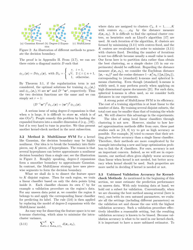
(a) Gaussian Kernel (b) Degree-2 Expan-sion
(c) MultiLinear
Figure 2: An illustration of di↵erent methods to gener-
ate the decision boundary.
The proof is in Appendix II. From (3.7), we can see
there exists a diagonal matrix D such that
�1,r(x) = D�1,1(x), with Dii =
8<
:
r, i = 1,pr, 2 i n+ 1,1, otherwise.
By Theorem 3.1, if the regularization term is not
considered, the optimal solutions for training �1,1(xi)
and �1,r(xi), 8i are w
⇤and D�1
w
⇤, respectively. Thus
the two decision functions are the same and we can
simply set r = 1:
(D�1w
⇤)
T�1,r(x) = (w
⇤)
T�1,1(x).
A serious issue of using degree-2 expansions is that
when n is large, it is di�cult to store w, which is of
size O(n2). People remedy this problem by hashing the
expanded features into a smaller dimension d (e.g., [19]),
but d is very hard to tune in practice. We thus present
another kernel-check method in the next subsection.
3.2 Method 2: MultiLinear SVM For a kernel
like Gaussian, the decision boundary may be highly
nonlinear. Our idea is to break the boundary into finite
pieces, say K pieces, of hyperplanes. The reason is that
several hyperplanes can better approximate a nonlinear
decision boundary than a single one; see the illustration
in Figure 2. Roughly speaking, degree-2 expansions
form a smoother boundary to approximate Gaussian.
In contrast, the MultiLinear strategy here uses piece-
wise segments to form the decision boundary.
What we shall do is to dissect the feature space
to K disjoint regions. Then for each region, we train
a linear classifier based on only the data points lying
inside it. Each classifier chooses its own C by for
example a validation procedure on the region’s data.
For any unseen data point x, we consider the region it
belongs to and apply the corresponding linear classifier
for predicting its label. The rule (3.6) is then applied
by replacing the model of degree-2 expansions with the
MultiLinear model.
An easy way for dissecting the feature space is to use
k-means clustering, which aims to minimize the intra-
cluster variance,
(3.11)
XK
k=1
Xxi2Ck
d(xi, ck),
where data are assigned to clusters Ck, k = 1, . . . ,Kwith centers c1, . . . , cK by the distance measure
d(xi, ck). It is di�cult to find the optimal cluster cen-
ters, so heuristics such as Lloyd’s algorithm [17] are
used. At each iteration of the algorithm, K clusters are
formed by minimising (3.11) with centres fixed, and the
K centres are recalculated in order to minimise (3.11)
with clusters fixed. Deciding the number of iterations
is not too di�cult because usually a small value is used.
Our focus here is to partition data rather than obtain
the best clustering, so a simple choice (15 in our ex-
periments) should be su�cient. Regarding the distance
measure d(xi, ck), we consider the Euclidean distance
kxi�ckk2 and the cosine distance 1�x
Ti ck/(kxikkckk),
corresponding to (standard) k-means and spherical k-
means clustering. Even though (standard) k-means is
widely used, it may perform poorly when applying on
high dimensional sparse documents [21]. For such data,
spherical k-means is often used, so we consider both
distances in our experiments.
A strong point of MultiLinear SVM is its e�ciency.
The cost of a training algorithm is at least linear to the
number of data. By training several disjoint subsets, the
total cost may be smaller than that of training the whole
set. We will observe this advantage in the experiments.
The idea of using local linear classifiers through
clustering is not new. However, similar to how ker-
nel approximation methods di↵er from ours, these past
studies such as [13, 8] try to get as high accuracy as
possible. For example, [8] tried to ensure that their set-
ting gives better accuracy than a single linear classifier.
Therefore, their methods are more complicated by for
example introducing a new and large optimization prob-
lem to link the K classifiers. For ours, accuracy is not
an important concern. Indeed, as we will see in exper-
iments, our method often gives slightly worse accuracy
than linear when kernel is not needed, but better accu-
racy when kernel should be used. Such properties are
more useful in deciding if kernel is needed or not.
3.3 Unbiased Validation Accuracy for Kernel-
check Methods As mentioned in the beginning of this
section, we must estimate the prediction performance
on unseen data. With only training data at hand, we
hold out a subset for validation. Conventionally, when
we are choosing the best method among several (here is
two), each with its own untuned parameters, we evalu-
ate all the settings (including di↵erent parameters) on
the validation set and choose the one with the highest
validation accuracy. Such a validation procedure e↵ec-
tively identifies a reasonable setting, but the resulting
validation accuracy is known to be biased. Because val-
idation accuracy is what to be used in our kernel-check,
it is important to have a more unbiased estimator. To

this end, we consider a two-stage validation process.
The training set is split to two parts T and V . Each
method did its own parameter selection on the set T ,and is then evaluated on the set V . Therefore, the set
V is dedicated only to get an accuracy estimation for
the kernel-checker. In our experiments we use a 3 to 1
split to generate the sets T and V .
4 Data Scaling for Linear Classification
We mentioned in Section 2.3 the di↵erent data scaling
methods used in linear and kernel classification. To see
if the same method can be applied, in this section we
investigate various scaling methods for linear classifica-
tion. In fact, we are not aware of any past study that
comprehensively addresses this issue. Our conclusion is
that the commonly used feature-wise scaling for kernel
is also suitable for linear.
4.1 Instance-wise Scaling Past studies did not
clearly explain why all instances need to be normal-
ized to unit vectors. For document data sets, a possi-
ble reason is to make short and long documents equally
important. In fact, a more compelling reason may be
related to the optimization method and the regulariza-
tion parameter C. Past developments (e.g., [10]) have
shown that for linear classification, low-order optimiza-
tion methods (e.g., coordinate descent methods) are ef-
ficient under small C, but may have slow convergence
under large C. One explanation is that when C is small,
we do not overfit the training data and the optimization
problem becomes easier. Interestingly, we show in the
following theorem that instance-wise normalization is a
mechanism to avoid using a large C.
Theorem 4.1. Suppose w is the optimal solution of
(2.1) under loss functions (2.2). If each instance xi
is changed to �xi, then w/� is optimal to the new
training set under the regularization parameter C/�2.
See proof in Appendix III. We consider two scenarios:
C = 1 with data xi, 8i versus C = 1 with xi/100, 8i.From the theorem, the former is equivalent to C =
10, 000 with data xi/100, 8i. Thus, under the default
C of any linear-classification package, instance-wise
normalization may help to avoid the slow convergence.
However, this normalization may not be needed if the
software can select a suitable C according to the size of
feature values. See more discussion in Section 4.3.
4.2 Feature-wise Scaling For linear classifiers, we
argue that the performance with/without feature-wise
scaling is about the same. Feature-wise scaling calcu-
lates Dxi+v, where D and v are constant diagonal ma-
trix and vector, respectively. Commonly we set v = 0 to
preserve the sparsity (e.g., each feature is divided by its
largest value). Then by Theorem 3.1, if the regulariza-
Table 1: Data statistics (density is calculated by using
the training set)
Data set l l (test) n density
a9a 32,561 16,281 123 11.3%
cod-rna 59,535 271,617 8 100%
covtype 581,012 NA 54 22.0%
fourclass 862 NA 2 100%
german.numer 1,000 NA 24 100%
gisette 6,000 1,000 5,000 99.1%
ijcnn1 49,990 91,701 22 59.1%
madelon 2,000 600 500 100%
mnistOvE 60,000 10,000 780 19.2%
news20 15,935 3,993 62,061 0.1%
poker 25,010 1,000,000 10 100%
rcv1 20,242 677,399 47,236 0.2%
real-sim 72,309 NA 20,958 0.2%
svmguide1 3,089 4,000 4 100%
webspam 350,000 NA 254 33.5%
tion term is not considered, the optimal solutions before
and after scaling are w
⇤and D�1
w
⇤, respectively. Thus
the two decision functions are the same.
4.3 Summary The discussion indicates that if suit-
able settings (e.g., proper C is chosen) have been con-
sidered, with/without scaling does not a↵ect the pre-
dictability much. Appendix V gives detailed experi-
ments to confirm this result. Then we need e�cient pa-
rameter selection regardless of the magnitude of feature
values. Fortunately, the recent study [3] has resolved the
issue for linear classification. For data in large numeric
ranges but not scaled, the approach in [3] can identify a
smaller C value without problem. Because feature-wise
scaling gives comparable results and is what used for
the Gaussian kernel, we perform this preprocessing step
before running all subsequent experiments.
In [3], by an e↵ective setting to select C, an
automatic procedure for linear classification is almost
there. We feel that the scaling issue is the last mile.
With the investigation in this section, a fully automated
process for linear classification is ready. Thus checking
if kernel is needed is naturally the next frontier.
5 Experiments
We conduct experiments to support the statements
discussed in Section 3, and to show the e↵ec-
tiveness and e�ciency of our proposed kernel-check
methods. Programs used for experiments are
available at http://www.csie.ntu.edu.tw/
~
cjlin/
papers/kernel-check, while more details of experi-
mental settings are in Appendix IV.
5.1 Data Sets and Performance Evaluation
We use 15 data sets (Available from LIBSVM
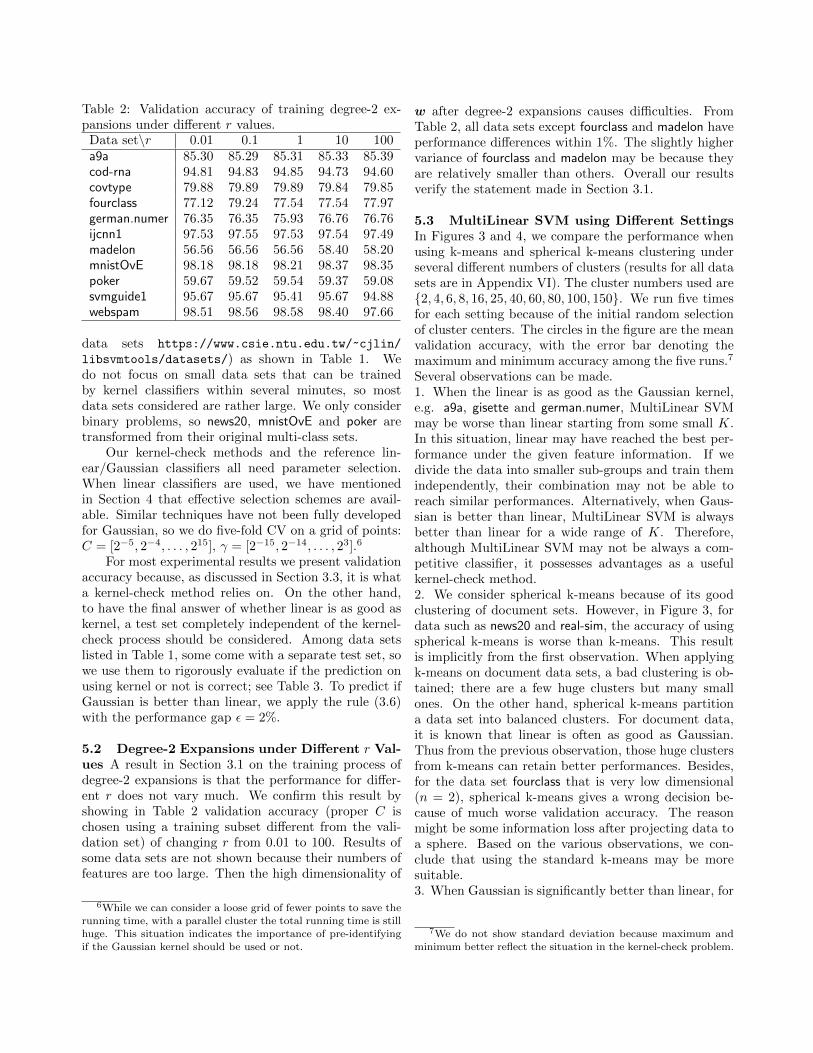
Table 2: Validation accuracy of training degree-2 ex-
pansions under di↵erent r values.
Data set\r 0.01 0.1 1 10 100
a9a 85.30 85.29 85.31 85.33 85.39cod-rna 94.81 94.83 94.85 94.73 94.60
covtype 79.88 79.89 79.89 79.84 79.85
fourclass 77.12 79.24 77.54 77.54 77.97
german.numer 76.35 76.35 75.93 76.76 76.76
ijcnn1 97.53 97.55 97.53 97.54 97.49
madelon 56.56 56.56 56.56 58.40 58.20
mnistOvE 98.18 98.18 98.21 98.37 98.35
poker 59.67 59.52 59.54 59.37 59.08
svmguide1 95.67 95.67 95.41 95.67 94.88
webspam 98.51 98.56 98.58 98.40 97.66
data sets https://www.csie.ntu.edu.tw/
~
cjlin/
libsvmtools/datasets/) as shown in Table 1. We
do not focus on small data sets that can be trained
by kernel classifiers within several minutes, so most
data sets considered are rather large. We only consider
binary problems, so news20, mnistOvE and poker are
transformed from their original multi-class sets.
Our kernel-check methods and the reference lin-
ear/Gaussian classifiers all need parameter selection.
When linear classifiers are used, we have mentioned
in Section 4 that e↵ective selection schemes are avail-
able. Similar techniques have not been fully developed
for Gaussian, so we do five-fold CV on a grid of points:
C = [2
�5, 2�4, . . . , 215], � = [2
�15, 2�14, . . . , 23].6
For most experimental results we present validation
accuracy because, as discussed in Section 3.3, it is what
a kernel-check method relies on. On the other hand,
to have the final answer of whether linear is as good as
kernel, a test set completely independent of the kernel-
check process should be considered. Among data sets
listed in Table 1, some come with a separate test set, so
we use them to rigorously evaluate if the prediction on
using kernel or not is correct; see Table 3. To predict if
Gaussian is better than linear, we apply the rule (3.6)
with the performance gap ✏ = 2%.
5.2 Degree-2 Expansions under Di↵erent r Val-
ues A result in Section 3.1 on the training process of
degree-2 expansions is that the performance for di↵er-
ent r does not vary much. We confirm this result by
showing in Table 2 validation accuracy (proper C is
chosen using a training subset di↵erent from the vali-
dation set) of changing r from 0.01 to 100. Results of
some data sets are not shown because their numbers of
features are too large. Then the high dimensionality of
6While we can consider a loose grid of fewer points to save therunning time, with a parallel cluster the total running time is stillhuge. This situation indicates the importance of pre-identifyingif the Gaussian kernel should be used or not.
w after degree-2 expansions causes di�culties. From
Table 2, all data sets except fourclass and madelon have
performance di↵erences within 1%. The slightly higher
variance of fourclass and madelon may be because they
are relatively smaller than others. Overall our results
verify the statement made in Section 3.1.
5.3 MultiLinear SVM using Di↵erent Settings
In Figures 3 and 4, we compare the performance when
using k-means and spherical k-means clustering under
several di↵erent numbers of clusters (results for all data
sets are in Appendix VI). The cluster numbers used are
{2, 4, 6, 8, 16, 25, 40, 60, 80, 100, 150}. We run five times
for each setting because of the initial random selection
of cluster centers. The circles in the figure are the mean
validation accuracy, with the error bar denoting the
maximum and minimum accuracy among the five runs.
7
Several observations can be made.
1. When the linear is as good as the Gaussian kernel,
e.g. a9a, gisette and german.numer, MultiLinear SVM
may be worse than linear starting from some small K.
In this situation, linear may have reached the best per-
formance under the given feature information. If we
divide the data into smaller sub-groups and train them
independently, their combination may not be able to
reach similar performances. Alternatively, when Gaus-
sian is better than linear, MultiLinear SVM is always
better than linear for a wide range of K. Therefore,
although MultiLinear SVM may not be always a com-
petitive classifier, it possesses advantages as a useful
kernel-check method.
2. We consider spherical k-means because of its good
clustering of document sets. However, in Figure 3, for
data such as news20 and real-sim, the accuracy of using
spherical k-means is worse than k-means. This result
is implicitly from the first observation. When applying
k-means on document data sets, a bad clustering is ob-
tained; there are a few huge clusters but many small
ones. On the other hand, spherical k-means partition
a data set into balanced clusters. For document data,
it is known that linear is often as good as Gaussian.
Thus from the previous observation, those huge clusters
from k-means can retain better performances. Besides,
for the data set fourclass that is very low dimensional
(n = 2), spherical k-means gives a wrong decision be-
cause of much worse validation accuracy. The reason
might be some information loss after projecting data to
a sphere. Based on the various observations, we con-
clude that using the standard k-means may be more
suitable.
3. When Gaussian is significantly better than linear, for
7We do not show standard deviation because maximum andminimum better reflect the situation in the kernel-check problem.

(a) fourclass (AC) (b) mnistOvE (AC) (c) webspam (AC) (d) madelon (AC)
(e) a9a (AC) (f) gisette (AC) (g) real-sim (AC) (h) news20 (AC)
Figure 3: Validation accuracy of MultiLinear SVM under di↵erent settings
(a) mnistOvE (Time) (b) webspam (Time) (c) a9a (Time) (d) news20 (Time)
Figure 4: Training time (including parameter search) of MultiLinear SVM under di↵erent settings
small K, MultiLinear SVM already has some improve-
ments over linear. This makes the problem of selecting
K easy. Further, training MultiLinear SVM is very ef-
ficient. For all data sets and all K values tried, the
training time is in the same order of magnitude as lin-
ear. Because intuitively a larger data set should be split
to more clusters, we think a setting like K = b5 ln(l)c(which is actually b5 ln(0.75l)c after taking the valida-
tion set out) might be appropriate. We will use this Kvalue in subsequent experiments.
5.4 Performance of Proposed Methods We
demonstrate the e�ciency and the e↵ectiveness of our
proposed method for checking whether linear is as good
as kernel. Table 3 shows the comparision results. A few
entries for degree-2 expansions are not given because
of the issue of high dimensionality. Although degree-2
expansions generally give correct decisions, the result
is wrong for madelon. A careful check shows that this
synthetic set contains 96% useless features generated
for a feature selection competition [9]. The degree-2 ex-
pansion adds many more useless features, so the perfor-
mance drops below linear. To illustrate this reasoning,
we add another data set, madelon(s), by eliminating use-
less features. Then the degree-2 expansion can give a
correct decision. On the other hand, the simple Mul-
tiLinear SVM correctly indicates for all 15 data sets if
the Gaussian kernel should be used.
6 Conclusion
We have studied the issue of deciding whether linear or
Gaussian kernel should be used. The aim is to make
this decision process a useful component for autoML.
Our proposed methods can e�ciently identify problems
for which a linear classifiers is as good as a kernel one, so
the training and testing time can be significantly saved.
References
[1] C.-C. Chang and C.-J. Lin. LIBSVM: A library forsupport vector machines. ACM TIST, 2(3):27:1–27:27,2011.
[2] Y.-W. Chang, C.-J. Hsieh, K.-W. Chang, M. Ring-gaard, and C.-J. Lin. Training and testing low-degree

Table 3: Performance of our proposed methods. Some abbreviations: val (validation accuracy in %), tme (time in
seconds), dec (using Gaussian or not?), accL (testing accuracy of linear in %), accK (testing accuracy of Gaussian
in %), Y (Yes), N (No), X (Not available) and U (Yes and No because the di↵erence is neither small nor large
enough). The value for MultiLinear SVM is averaged over five runs. The columns of “True answer” are by using
an independent test set that is not involved in the kernel-check process.
Linear Degree-2 MultiLinear Kernel True answer
data set val tme val tme dec K val tme dec val dec accL accK dec
ijcnn1 92.4 11.22 97.5 28.47 Y 52 98.3 2.54 Y 98.6 Y 91.8 98.4 Y
madelon 58.6 18.09 56.6 3,969.30 N 36 68.4 2.75 Y 67.2 Y 59.7 67.7 Y
madelon(s) 62.4 0.23 68.0 20.02 Y 36 77.4 0.34 Y 78.7 Y 59.0 78.3 Y
mnistOvE 89.2 304.79 98.2 2,635.86 Y 53 97.0 26.10 Y 99.1 Y 89.8 99.1 Y
poker 50.0 0.85 59.5 11.79 Y 49 55.1 0.96 Y 61.3 Y 50.0 61.7 Y
svmguide1 82.9 0.05 95.4 0.16 Y 38 95.4 0.06 Y 96.4 Y 78.9 96.6 Y
webspam 92.7 713.23 98.6 11,476.02 Y 62 97.7 204.79 Y 99.1 Y NA NA X
fourclass 75.0 0.01 77.5 0.03 Y 32 97.3 0.02 Y 100.0 Y NA NA X
covtype 75.7 615.97 79.9 9,949.78 Y 64 80.9 51.42 Y 96.1 Y NA NA X
a9a 85.1 5.04 85.3 195.3 N 50 84.7 2.85 N 84.9 N 85.0 85.1 N
gisette 96.6 148.84 NA NA X 42 95.5 86.23 N 97.1 N 98.0 98.0 N
news20 90.2 648.02 NA NA X 46 90.1 497.63 N 88.6 N 90.2 87.9 N
rcv1 96.6 44.07 NA NA X 48 96.7 53.72 N 97.2 N 96.1 94.9 N
real-sim 97.7 100.23 NA NA X 54 97.4 101.84 N 97.8 N NA NA X
german.numer 77.2 0.10 75.9 28.54 N 33 68.5 0.13 N 77.3 N NA NA X
cod-rna 93.2 4.36 94.8 17.18 U 53 95.0 1.80 U 95.9 U 95.0 96.4 U
polynomial data mappings via linear SVM. JMLR,11:1471–1490, 2010.
[3] B.-Y. Chu, C.-H. Ho, C.-H. Tsai, C.-Y. Lin, and C.-J. Lin. Warm start for parameter selection of linearclassifiers. In KDD, 2015.
[4] C. Cortes and V. Vapnik. Support-vector network.MLJ, 20:273–297, 1995.
[5] R.-E. Fan, K.-W. Chang, C.-J. Hsieh, X.-R. Wang,and C.-J. Lin. LIBLINEAR: a library for large linearclassification. JMLR, 9:1871–1874, 2008.
[6] M. Fernandez-Delgado, E. Cernadas, S. Barro, andD. Amorim. Do we need hundreds of classifiers to solvereal world classification problems? JMLR, 15:3133–3181, 2014.
[7] S. Fine and K. Scheinberg. E�cient SVM trainingusing low-rank kernel representations. JMLR, 2:243–264, 2001.
[8] Q. Gu and J. Han. Clustered support vector machines.In AISTATS, 2013.
[9] I. Guyon, S. Gunn, A. B. Hur, and G. Dror. Resultanalysis of the NIPS 2003 feature selection challenge.In NIPS. 2005.
[10] C.-J. Hsieh, K.-W. Chang, C.-J. Lin, S. S. Keerthi, andS. Sundararajan. A dual coordinate descent method forlarge-scale linear SVM. In ICML, 2008.
[11] C.-W. Hsu, C.-C. Chang, and C.-J. Lin. A practicalguide to support vector classification. Technical report,National Taiwan University, 2003.
[12] S. S. Keerthi and C.-J. Lin. Asymptotic behaviors ofsupport vector machines with Gaussian kernel. Neural
Comput., 15(7):1667–1689, 2003.[13] L. Ladicky and P. H. S. Torr. Locally linear support
vector machines. In ICML, 2011.
[14] Q. Le, T. Sarlos, and A. Smola. Fastfood - approxi-mating kernel expansions in loglinear time. In ICML,2013.
[15] Y.-J. Lee and O. L. Mangasarian. RSVM: Reducedsupport vector machines. In SDM, 2001.
[16] R. A. Lippert and R. M. Rifkin. Infinite-� limits forTikhonov regularization. JMLR, 7:855–876, 2006.
[17] S. Lloyd. Least squares quantization in PCM. IEEE
Trans. Inf. Theor., 28:129–137, 1982.[18] D. Meyer, F. Leisch, and K. Hornik. The support
vector machine under test. Neurocomputing, 55:169–186, September 2003.
[19] N. Pham and R. Pagh. Fast and scalable polynomialkernels via explicit feature maps. In KDD, 2013.
[20] A. Rahimi and B. Recht. Random features for large-scale kernel machines. NIPS, 2008.
[21] A. Strehl, J. Ghosh, and R. Mooney. Impact ofsimilarity measures on web-page clustering. In AAAI
Workshop on AI for Web Search, 2000.[22] V. Vapnik. Statistical Learning Theory. Wiley, New
York, NY, 1998.[23] C. K. I. Williams and M. Seeger. Using the Nystrom
method to speed up kernel machines. In NIPS, 2001.[24] H.-F. Yu, F.-L. Huang, and C.-J. Lin. Dual coordinate
descent methods for logistic regression and maximumentropy models. MLJ, 85:41–75, 2011.
[25] G.-X. Yuan, C.-H. Ho, and C.-J. Lin. Recent advancesof large-scale linear classification. PIEEE, 100:2584–2603, 2012.
[26] K. Zhang, L. Lan, Z. Wang, and F. Moerchen. Scalingup kernel SVM on limited resources: A low-ranklinearization approach. In AISTATS, 2012.


![A Kernel Classification Framework for Metric Learningcslzhang/paper/SVMML.pdf · kernel learning, and proposed a framework for metric learning with multiple kernels [21]. In our](https://img.dokumen.tips/doc/110x75/5fcc922fcbb0c45e3b76fd9e/a-kernel-classiication-framework-for-metric-cslzhangpapersvmmlpdf-kernel.jpg)