Proceedings of the Cold-Formed Steel Research Consortium Colloquium20-22 October, 2020 (cfsrc.org)

Linear and bifurcation analyses combining shell and GBT-based beam finite elements

David Manta1, Rodrigo Goncalves2, Dinar Camotim3

Abstract

This paper concerns a general and very efficient approach to model thin-walled members with complex geometries (includingtaper and/or connected through joints), which combines standard shell and GBT-based finite elements. This approach (i)allows a straightforward modelling of complex geometries and (ii) is very efficient from a computational point of view, asthe shell model substructures can be condensed out of the global equilibrium equations. The capabilities of the proposedapproach are demonstrated through several examples concerning the linear and bifurcation (linear stability) analyses of(i) members with tapered segments, (ii) members with holes and (iii) beam-column assemblies. The results obtained arecompared with full shell finite element model solutions and an excellent match is obtained.

1. Introduction

Generalised Beam Theory (GBT) is nowadays well-established as an efficient tool to analyse thin-walled barssubjected to global/distortional/local deformation. Its mainadvantages arise from the modal decomposition of the beamkinematics in a set of so-called “cross-section deformationmodes”, which constitute a distinct feature of GBT and leadto accurate solutions even when just a few of them are usedin the analysis. This leads to major computational gains,which are particularly evident in the context of linear and bi-furcation (linear stability) analyses.

Since the pioneer works of Schardt [1], [2] (see http://vtb.infofor a complete list of publications of the Darmstad-basedgroup), GBT has been considerably developed by severalresearchers, most notably the Lisbon-based research group(see, e.g. [3], [4] and http://www.civil.ist.utl.pt/gbt for an up-dated list of publications). GBT constitutes an extension ofthe Vlasov prismatic bar theory and therefore its applicationto non-prismatic members is not straightforward. In this re-spect the following research efforts are worth mentioning.Moderately tapered members are treated in [5] and coni-cal shells in [6], [7]. Members with holes have been ad-

1CERIS and Departamento de Engenharia Civil, Faculdade de Cienciase Tecnologia, Universidade Nova de Lisboa, 2829-516, Caparica, Portugal,d.manta@campus.fct.unl.pt

2CERIS and Departamento de Engenharia Civil, Faculdade de Cienciase Tecnologia, Universidade Nova de Lisboa, 2829-516, Caparica, Portugal,rodrigo.goncalves@fct.unl.pt

3CERIS, ICIST, DECivil, Instituto Superior Tecnico, Universidade de Lis-boa, Av. Rovisco Pais, 1049-001 Lisboa, Portugal, dcamotim@civil.ist.utl.pt

dressed in [8], although at the expense of requiring a refinedcross-section discretisation (and only the membrane longitu-dinal normal pre-buckling stresses are taken into account).A general approach for members with holes, discrete thick-ness variation, plasticity and geometrical non-linearity wasproposed in [9], using non-orthogonal deformation modes toimprove the computational efficiency (the orthogonal modesare retrieved through post-processing the results). A linearformulation for members with circular axis was proposed in[10], [11]. Finally, frames have been dealt with using carefullychosen constraints between connecting members [12]–[15].

This paper proposes an alternative and more general ap-proach, where shell and GBT-based (beam) finite elementsare combined to allow handling, rather straightforwardly,complex geometries. In essence, the GBT elements areused to model prismatic members, while shell elements areadopted in the remaining zones (tapering, holes, joints, etc.).This subdivision makes it possible to include only a smallnumber of deformation modes in the GBT elements with-out sacrificing accuracy, since the zones with concentratedstresses/strains, usually requiring many deformation modesto be correctly modelled with GBT, are handled by the shellelements. Although this paper addresses linear (first-order)and bifurcation (linear stability) analyses, since the GBT ap-proach is most effective in this context, the procedure is cur-rently being extended by the authors to cover other analysistypes.

The outline of the paper is as follows. Section 2 presents thefundamentals of the adopted GBT-based and shell finite ele-ments. Section 3, discusses the procedure adopted for com-

bining GBT and shell elements. Next, Section 4 presentsthree numerical examples that demonstrate the capabilitiesof the proposed approach. For comparison purposes, solu-tions obtained with full shell finite element models are pro-vided. Finally, the paper closes in Section 5, with the con-cluding remarks.

2. The adopted shell and GBT-based finite elements

This section presents the fundamentals of the selected shelland GBT-based finite elements, as well as their combina-tion. Concerning the notation, scalars are represented initalic letters and vectors/matrices in bold letters. The usualidentity matrix is displayed as 1 and matrices/vectors withnull entries as 0. The standard Euclidean inner product be-tween two vectors of arbitrary dimension a and b is writtenas a · b, a derivative is represented by a subscript comma(e.g. f,a = ∂f/∂a), a virtual variation is denoted by δ andan incremental variation by ∆. Moreover, h is the shell/wallthickness.

In the present work, Green-Lagrange strains E are adopted,together with their work-conjugate second Piola-Kirchhoffstresses S. Therefore, using a Voigt-like notation, the equilib-rium equations are obtained from the virtual work statement

δW = −∫V

δE · S dV +

∫Ω

δU · q dΩ = 0, (1)

where V and Ω are the thin-walled member volume and mid-surface, respectively, at the initial configuration, and it is as-sumed that the external loads, q, are applied at the ele-ment mid-surface only, where U are the work-conjugate mid-surface displacements.

In addition, a linear elastic stress-strain relation is assumed,of the form

S = CE, (2)

where C is the constitutive matrix. A St. Venant-Kirchhoffmaterial law is adopted, written in terms of Young’s modulusE, the shear modulus G and Poisson’s ratio ν.

Next, a distinction is made between two cases. Firstly, thelinear analysis case, where Green-Lagrange strains becomesmall strains ε and the internal virtual work is given by

δWint = −∫V

δε ·Cε dV. (3)

Secondly, the linear stability analysis case is considered. Apreliminary linear pre-buckling analysis must be performed toretrieve the pre-buckling stresses. Recalling that thin-walledmembers are being addressed, both the shell and GBT for-mulations used in this work only retain the membrane partof these stresses, S. Therefore, the linearisation of Equation

Figure 1: MITC-4 reference systems and displacement components.

(1) at the initial configuration leads to the bifurcation equation

∆δWint(φ = 0, λ) = −∫V

(δε ·C∆ε+ ∆δE · λS

)dV, (4)

where φ is a vector that collects the kinematic variables (withφ = 0 referring to the initial configuration) and λ is the loadmultiplier, which is assumed to be directly proportional to thestresses S (calculated for λ = 1). The first and second termsin Equation (4) lead to the finite element linear and geometricstiffness matrices, respectively.

2.1 The MITC-4 shell finite element

In this work, a 4-node shell finite element with a Reissner-Mindlin kinematic description is adopted. It is well knownthat, in this case, a pure displacement-based interpolationwill lead to shear locking. This phenomenon is circumventedusing the Mixed Interpolation of Tensorial Component (MITC)strategy developed by Bathe and co-workers (see, e.g., [16],[17]). According to Figure 1, three reference systems aredefined: (i) the global Cartesian system (X, Y , Z), (ii) theelement Cartesian local axes (x, y, z), where x is attached toone of the element lateral faces, and (iii) a convected frame(r, s, t), where t is assumed coincident with the local z axis,defining the through-thickness direction (the shell is initiallyflat).

Following the Reissner-Mindlin hypothesis, the mid-surfacedisplacements u, v, w and the rotations θx, θy along the localaxes (see Figure 1) constitute the necessary and sufficientkinematic variables to completely describe the element dis-placement field U , through

U(x, y, z) =

UxUyUz

=

u(x, y) + zθy(x, y)v(x, y) − zθx(x, y)

w(x, y)

. (5)

In the local Cartesian system, adopting Voigt-like vectorforms, the Green-Lagrange strains are subdivided into mem-brane (M ), bending (B) and shear (S) components, and only

2

the non-linear part of the membrane components is retained,reading

EM =

EMxxEMyy2EMxy

=

u,xv,y

u,y + v,x

+1

2

U ,x · U ,x

U ,y · U ,y

2U ,x · U ,y

, (6)

EB =

EBxxEByy2EBxy

= z

θy,x−θx,y

θy,y − θx,x

, (7)

ES =

[2Exz2Eyz

]=

[w,x + θyw,y − θx

], (8)

with UT= [u v w] being the mid-surface displacement vec-

tor. Although membrane locking is not present in the con-text of linear and bifurcation analyses (the element is initiallyflat), shear locking may occur and is mitigated with the MITCapproach by re-interpolating the covariant through-thicknessshear strains from their values at the so-called “tying points”(see [17], [18] for details).

Concerning the stresses, a plane stress state is assumed(Szz = 0), leading to

SM = CEM , SB = CEB , SS = GES , (9)

C =E

1 − ν2

1 ν 0ν 1 00 0 1−ν

2

. (10)

The finite element equations are obtained by interpolatingthe mid-surface displacements and rotations using linearfunctions and following a standard isoparametric approach.The independent kinematic variables are collected in the vec-tor

φT =[u v w θx θy

], (11)

and the interpolation is then given by φ = Ψd, where Ψ is amatrix containing the interpolation functions

ΨT =[ψTu ψTv ψTw ψTθx ψTθy

], (12)

where ψ(·) are the suitable sub-matrices that match the com-ponents of the vector of nodal unknowns

dT =[u1 v1 w1 (θx)1 (θy)1 . . .

. . . u4 v4 w4 (θx)4 (θy)4

]. (13)

For a linear analysis, recalling Equation (3), the element stiff-ness matrix is given by

Ke =

∫V

(BTM CBM +BT

BCBB +GBTSBS

)dV, (14)

were the full expressions of the strain-displacement matricesBM , BB are given in [18] and BS can be found in [16].

Lastly, for the linear stability analyses, from the final term ofEquation (4), the element geometric matrix is obtained as

Ge = λ

∫V

(SMxxB

TxxBxx + SMyyB

TyyByy+

+ SMxy

(BTxxByy + B

TyyBxx

))dV, (15)

with the auxiliary matrices Bxx and Byy being provided in[18].

For the computation of these matrices, numerical integrationis performed using a 2 × 2 Gauss point grid along the shellmid-surface. Along the thickness direction, since only elasticexamples are addressed in this paper, analytical integrationis performed.

2.2 The GBT-based finite element

The GBT element employed in this work follows that pro-posed in [19], although some simplifications are introduced,namely: (i) geometrical imperfections are disregarded, (ii)simplifications are introduced to the membrane stress andstrain fields, (iii) a linear elastic material is assumed and(iv) in the context of a linear stability analysis, only the non-linear strain terms associated with the membrane longitudi-nal extensions are considered, which is acceptable for slen-der bars.

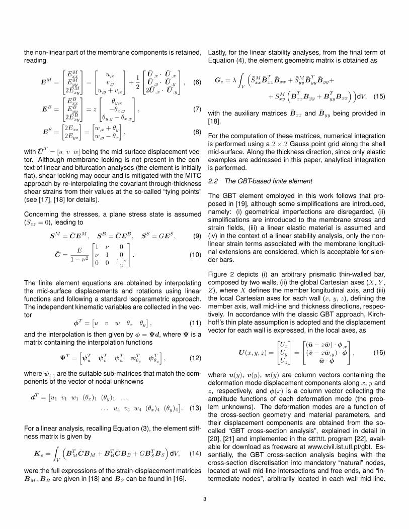
Figure 2 depicts (i) an arbitrary prismatic thin-walled bar,composed by two walls, (ii) the global Cartesian axes (X, Y ,Z), where X defines the member longitudinal axis, and (iii)the local Cartesian axes for each wall (x, y, z), defining themember axis, wall mid-line and thickness directions, respec-tively. In accordance with the classic GBT approach, Kirch-hoff’s thin plate assumption is adopted and the displacementvector for each wall is expressed, in the local axes, as

U(x, y, z) =

UxUyUz

=

(u− zw) · φ,x(v − zw,y) · φ

w · φ

, (16)

where u(y), v(y), w(y) are column vectors containing thedeformation mode displacement components along x, y andz, respectively, and φ(x) is a column vector collecting theamplitude functions of each deformation mode (the prob-lem unknowns). The deformation modes are a function ofthe cross-section geometry and material parameters, andtheir displacement components are obtained from the so-called “GBT cross-section analysis”, explained in detail in[20], [21] and implemented in the GBTUL program [22], avail-able for download as freeware at www.civil.ist.utl.pt/gbt. Es-sentially, the GBT cross-section analysis begins with thecross-section discretisation into mandatory “natural” nodes,located at wall mid-line intersections and free ends, and “in-termediate nodes”, arbitrarily located in each wall mid-line.

3

X

Y

Z

Figure 2: Arbitrary thin-walled member geometry, global/local coordinatesystems and local displacement components.

The in-plane/warping displacements of these nodes consti-tute the basis for the definition of the cross-section deforma-tion modes. Subsequently, an appropriate change of basis isperformed to obtain a hierarchical and structurally meaning-ful set of deformation modes.

In a linear analysis context, the non-null small strain compo-nents (for each wall) are stored in vector ε, reading

ε =

εxxεyyγxy

=

(u− zw) · φ,xx(v,y − zw,yy) · φ

(u,y + v − 2zw,y) · φ,x

, (17)

where the membrane/bending terms are constant/linearalong the thickness direction z, respectively.

With the purpose of reducing the deformation modes in-cluded in the analyses, without compromising accuracy, inbeam-type problems two constraints are usually adopted: (i)null membrane transverse strains (εMyy = 0) and (ii) null mem-brane shear strains (γMxy = 0, the so-called Vlasov’s assump-tion). These two assumptions are always employed in thispaper, recalling that the contribution of this work consistsof modelling (i) complex zones with shell elements and (ii)the remaining (prismatic) zones with GBT elements includ-ing just a few deformation modes. With the above strain con-straints, only two deformation mode sets are obtained: (i)natural Vlasov modes (axial extension, bending, torsion andseveral distortional modes) and (ii) local-plate modes.

For the calculation of bifurcation loads, only the Green-Lagrange longitudinal membrane strains are required, as al-ready mentioned. The relevant Green-Lagrange strains are

therefore grouped in vector ET = [Exx εyy γxy]T , with

EMxx = εxx +1

2

(φT,x

(vvT + wwT

)φ,x + φT,xxuu

Tφ,xx

).

(18)In addition, the term uuT may be discarded without signifi-cant loss of accuracy [23].

For the stresses, a plane stress state is assumed, with ST =[Sxx Syy Sxy]. However, due to the null transverse membranestrain constraint, the membrane and bending stresses areseparated in order to avoid over-stiff solutions, leading to

SM = CMEM , SB = CEB , (19)

CM =

E 0 00 0 00 0 0

. (20)

The finite element is obtained by interpolating the amplitudefunctions by means of Hermite cubic polynomials for all de-formation modes except those involving only warping (e.g.,the axial extension mode), in which case quadratic Lagrangefunctions are employed. As in the case of the shell elements,the interpolation is of the form φ = Ψd, where matrix Ψ con-tains the interpolation functions and d is the vector of un-knowns.

For a linear analysis, from (3), the element stiffness matrixreads

Ke =

∫L

ΨΨ,x

Ψ,xx

T B 0 D2

0 D1 0

DT2 0 C

ΨΨ,x

Ψ,xx

dx, (21)

where L is the member initial length and the GBT modal ma-trices are given by

B =

∫S

Eh3

12(1 − ν2)w,yyw

T,yy dy, (22)

C =

∫S

(EhuuT +

Eh3

12(1 − ν2)wwT

)dy, (23)

D1 =

∫S

Gh3

3w,yw

T,y dy, (24)

D2 =

∫S

νEh3

12(1 − ν2)w,yyw

T dy, (25)

where S is the cross-section mid-line. It is worth-noting thatmembrane/bending terms are multiplied by h/h3, respec-tively.

Finally, for linear stability analyses, from Equation (4), theelement geometric matrix reads

Ge = λ

∫L

∫S

hSMxxΨT,x(vvT + wwT )Ψ,xdy dx. (26)

4

3. Combining shell and GBT-based finite elements

As previously mentioned, the focus of the proposed ap-proach is to combine the versatility of shell elements to modelzones (shell substructures or macro-elements) where a com-plex behaviour is expected, with the computational efficiencyof the GBT-based elements to model the regular/smoothzones, where just a few deformation modes are required tocapture the beam displacement field.

As an illustrative example, Figure 3 depicts an assembly oftwo GBT-based (beam) finite elements and a shell macro-element, concerning a single beam wall. The connection de-tail shows (i) “linked nodes” (nodes shared by the shell andGBT models) and also (ii) “hanging nodes” (see, e.g., [24]),which appear due to the fact that the cross-section discreti-sation is generally coarser in the GBT model. In general,the constraint equations should apply to both types of nodes,to ensure compatibility. However, if the shell macro-elementzone is extended so that severe localized deformation doesnot occur at the GBT-shell interface, the constraints for thehanging nodes can be discarded without significant loss ofaccuracy. This approach is followed in this work, being fur-ther discussed in Section 4.

At a boundary connecting shell and GBT elements, compat-ibility is enforced through constraint equations of the form

ζj(USFEkj (z = 0) − UGBTkj (z = 0)

)= 0, (27)

where ζj are Lagrange multipliers and UGBTkj , USFEkj are thedisplacements of the mid-surface (z = 0) node k along di-rection j, in the GBT and shell discretisations, respectively.Since only the mid-surface nodal displacements are con-strained (i.e., the shell nodal rotation DOFs are not con-strained), this procedure leads to a loss of compatibilityacross the shell/GBT interface. However, this issue has littlerelevance for thin-walled members, where through-thicknessshearing is generally negligible. If this effect is important,it must be minimized by extending the shell macro-elementzone — this issue will be addressed in the numerical exam-ples presented in Section 4.

The constraint equations can be cast as

ζT (BSFE dSFE −BGBT dGBT ) = 0, (28)

where ζ is a column vector collecting all the Lagrange mul-tipliers, dSFE and dGBT are the components of vector d ofthe shell and GBT finite elements, respectively, and the aux-iliary matrices BSFE and BGBT contain the coefficients ofthe constraint equations.

Matrix BSFE can be obtained by introducing a single unitentry at each row, corresponding to the selected shell dis-placement to constrain. For the computation of matrixBGBT ,

Figure 3: Coupling between a shell macro-element and two GBT finite ele-ments.

the deformation modes are first calculated using GBTUL andthen Equation (16) is employed to calculate the correspond-ing displacement, with z = 0 (mid-line) and φ = ΨdGBT .Naturally, if the axes do not match, a coordinate transforma-tion is necessary.

The resulting equation system reads

KSFE 0 BTSFE

0 KGBT −BTGBT

BSFE −BGBT 0

dSFEdGBTζ

=

F SFEFGBT0

, (29)

where KSFE and KGBT are the global stiffness matrices ofthe shell macro-element and GBT-based finite elements, re-spectively, and F SFE , FGBT are the associated nodal forcevectors. Although the system is symmetric, matrices BSFE

and BGBT are generally neither symmetric nor square.

The system (29) can be simplified by eliminating the La-grange multipliers and condensing the shell macro-elementDOFs, leading to a system involving only the GBT DOFs.Besides leading to a great economy of DOFs, this procedureis particularly useful if a shell macro-element library is avail-able in the code (i.e., the linear stiffness matrices of severaltypes of member connections are already available) and/orthe macro-elements appear at several locations in the model(which is typical in steel structures).

For the bifurcation problem, the same principles apply. Sev-eral numerical techniques for condensing DOFs are available(see, e.g., [25]), the simplest one consisting of setting thecorresponding sub-matrices ofG to zero, which is equivalentto the standard static condensation of massless DOFs in alumped mass model, for the calculation of natural frequen-cies. However, since the examples presented in this paper donot involve many DOFs, no condensation of the shell DOFswas performed.

5

4. Numerical examples

4.1 Lipped channel cantilever with a tapered segment

The first example concerns a lipped channel cantilever beamwith a tapered segment. Figure 4 (a) shows the beam geom-etry and material parameters. The height of the tapered partof the beam varies linearly for 0 ≤ X ≤ 0.25 m, remainingconstant thereafter.

The GBT cross-section discretisation employed is shown inFigure 4 (a). With this discretisation, 39 deformation modesare obtained. As mentioned before in Section 2.2, only thenatural Vlasov (modes 1 to 6) and local-plate modes (modes7 to 15) are included in the analyses (see Figure 4 (b)).

Three models are analysed: (i) a full shell model with 2220elements, (ii) a less refined GBT-shell model, where only thetapered zone is discretised with a shell macro-element (550shell elements + 10 GBT elements), and (iii) a refined GBT-shell model where the shell macro-element is extended 0.25m into the uniform height zone (1100 shell elements + 5 GBTelements).

Figure 5 (a) displays the linear analysis results, namely thedeformed configurations, the GBT mode amplitude diagramsand the displacements of points P1 and P2 identified in thisfigure (the differences with respect to the full shell model arealso displayed).

Concerning the displacements of points P1 and P2, the re-sults show that both GBT-shell solutions match very accuratethe full shell model one (differences below 1%), a fact whichis confirmed by the very good agreement between the de-formed configurations displayed in the figure.

The mode amplitude diagrams make it possible to concludethat minor axis bending (mode 3) and symmetric distortion(mode 5) are the most important. In fact, the deformed con-figurations provided in the figure clearly corroborate this re-mark. Near the transition zone, for the less refined GBT-shellmodel, several local-plate modes also appear, even if theircontributions are at least one order of magnitude below thoseof modes 3 and 5 (these participations are hardly noticeablein the diagram, near x = 0). On the other hand, the modalparticipation diagram of the refined GBT-shell model is es-sentially a truncated version of the less refined one. Con-sequently, the local-plate modes in the tapered-uniform tran-sition zone no longer appear. This shows that, as pointedout in Section 3, extending the shell macro-element zone in-creases the dissipation of local deformation effects stemmingfrom the transition and, furthermore, makes it possible to useless deformation modes in the GBT-based element (in thiscase, it is possible to discard the local-plate modes).

Next, a linear stability analysis of the cantilever is carried outto determine the first buckling load (the load profile consistsof 2×1 kN point loads) and the corresponding buckling mode.Once more, the previous three models are considered (seeFigure 5 (b)).

In this case, the mode amplitude diagrams show that thebuckling modes are essentially distortional, although majoraxis bending also participates along the beam, and local-plate modes appear near the GBT-shell transition zone. TheGBT-shell refined model leads to a bifurcation load nearly co-incident to the full shell model. Once more, the benefits of ex-tending the shell macro-element beyond the tapered-uniformtransition zone are clear: accuracy increases and the partic-ipations of the local-plate modes become much smaller. It isworth remarking that the buckling loads obtained by the GBT-shell models are slightly lower than those provided by the fullshell model as a consequence of the lack of complete com-patibility along the GBT-shell interface. Nevertheless, the dif-ferences obtained are very small for the extended GBT-shellmodel (1.33%).

4.2 Lipped channel cantilever with two long holes

The second example consists of a lipped channel cantileverwith the same material parameters and cross-section of theuniform segment of the previous example (see Figure 4 (a)),but having two long holes located exactly in the middle ofeach flange. The beam geometry is displayed in Figure 6.Concerning the loadings, the linear analysis is performed fora 1 kN lateral load (along −Y ), applied at one of the flange-lipcorners near the cantilever mid span, whereas for the bifur-cation analysis the loading consists of a 1 kN load applied atthe flange-web corner of the free-end section, along −Z.

Three models are considered: (i) a shell model without theholes, to assess their influence (1650 elements), (ii) a shellmodel with the holes (1590 elements) and (iii) a GBT-shellmodel where a shell macro-element is employed for the 0.55m central segment of the beam (660 shell elements + 10GBT elements). The linear and bifurcation analyses resultsare reported in Figure 7.

The linear analysis results are first examined. A comparisonbetween the shell models depicted in Figure 7 (a) with andwithout holes shows that the latter yields a much stiffer re-sponse, providing a 73% lower lateral displacement of thepoint of load application. The GBT-shell model captures theshell model (with holes) deformed configuration very accu-rately, with a small difference (2%) in terms of the displace-ment of the point of load application. Furthermore, the modalparticipation diagrams provided in the figure make it possi-ble to conclude that the zones without the holes undergo es-sentially major-axis bending (mode 2), torsion and symmetric(mode 5) plus anti-symmetric (mode 6) distortion. The con-

6

Figure 4: Lipped channel cantilever: (a) geometry and GBT cross-section discretisation, and (b) first 15 cross-section deformation modes.

tributions of local-plate modes are virtually null.

Consider now the bifurcation analysis results displayed inFigure 7 (b). The holes play again a very significant role,namely in the critical load parameter, which is more than 20%higher in their absence, and in the buckling mode shapes:(i) with holes, the mode is characterised by a pronounceddistortion in the right hole zone, with a significant inwardlateral displacement of the lip, whereas (ii) without holes,cross-section distortion mostly occurs near the support. TheGBT-shell model captures the buckling mode quite accuratelyand provides a critical load which falls within 2% of the shellmodel one.

The modal participation diagrams concerning the bucklingmode make it possible to conclude that both segments with-out holes essentially undergo distortion (modes 5 and 6) andthat the free end zone also exhibits bending and some tor-sion.

4.3 L-shaped frame with a tapered joint

The third and last example consists of the L-shaped framedepicted in Figure 8 (a). The joint has a complex tapered ge-ometry that influences significantly the frame structural be-haviour. Consequently, the joint zone is discretised with ashell macro-element. Concerning the loadings, the linearanalysis is carried out with an eccentric 10 kN vertical force,

applied at the flange outstand of the free end, whereas forthe bifurcation analysis the force is changed to a 1 kN loadand moved to the top web-flange intersection. It is also worthnoting that, in the bifurcation analysis, two lateral supportsare provided at the free end cross-section, in order to obtaina buckling mode involving complex lateral-torsional-local dis-placements at the joint (otherwise the critical buckling modeessentially involves lateral-torsional buckling of the horizontalbeam).

The GBT the cross-section discretisation shown in Figure 8(a) is adopted, involving a single intermediate node in theweb. The relevant deformation modes included in the GBTfinite element are displayed in Figure 8 (b) and consist of only4 natural Vlasov and 5 local-plate modes.

Figure 9 shows the results of the linear and bifurcation anal-yses. In both cases two models are compared: (i) a shellmodel (2801 elements) and (ii) a GBT-shell model (1151 shellelements + 10 GBT elements).

The linear analysis results show that, in spite of the complex-ity of the structure, the GBT-shell model yields a vertical dis-placement of the point of load application which is virtuallyidentical to that provided by the shell model (0.17% differ-ence). The GBT mode amplitude diagrams provided on theright of Figure 9 (a) show that the vertical member essen-tially undergoes in-plane and out-of-plane bending, whereas

7

Figure 5: Lipped channel cantilever: (a) linear analysis and (b) bifurcation analysis (first buckling load).

8

Figure 6: Lipped channel cantilever with two long holes.

the horizontal beam exhibits a more complex behaviour, in-volving mostly bending and torsion, but also local effects nearthe free end, due to the influence of the point load. Also notethat, in the horizontal member, the axial extension mode hasa constant participation, which indicates that, as expected, itundergoes a rigid-body horizontal displacement.

Concerning the bifurcation results shown in Figure 9 (b), itshould be first noted that the critical buckling mode exhibits avery complex behaviour at the joint, which can only be ad-equately captured with shell elements. Nevertheless, theproposed GBT-shell approach yields excellent results, witha critical load difference of only 3.5%. The modal participa-tion diagrams make it possible to conclude that the bucklingbehaviour of the prismatic members is almost purely global(i.e., the local-plate modes have almost null participations),thus confirming that the complex behaviour is restricted tothe joint zone.

5. Concluding remarks

This paper presented an efficient approach to analyse thin-walled members with complex geometries and connections,combining standard shell and GBT-based finite elements.The GBT elements are used to model prismatic member seg-ments, whereas the complex zones (discontinuities, holes,joints, etc.) are dealt with using shell elements, creating shellmacro-elements. For this approach, two major advantagescan be pointed out: (i) the number of deformation modes em-ployed in the GBT elements can be reduced and (ii) the shellmacro-elements can be condensed out of the global equilib-rium equation system, leading to a very high DOF economyand ensuring fast computation times. The latter advantage isespecially important if the complete structure involves manyidentical macro-elements.

For validation and illustrative purposes, three numerical ex-amples were presented and discussed, concerning (i) alipped channel cantilever with a tapered segment, (ii) a lippedchannel cantilever with long flange holes and (iii) an L-shaped frame with a tapered joint. Linear and bifurcation(linear stability) analyses were carried out in all cases andthe results obtained with the proposed approach were com-pared with full shell models. All the cases shown an excellentagreement.

As a final note, it is mentioned that the authors are currentlyextending this approach to other types of structural analyses.

6. Acknowledgments

The first author gratefully acknowledges the financial supportof FCT (Fundacao para a Ciencia e a Tecnologia, Portugal),through the doctoral scholarship SFRH/BD/130515/2017.

References

[1] R. Schardt, “Eine Erweiterung der Technis-chen Biegetheorie zur Berechnung prismatischerFaltwerke”, Stahlbau, vol. 35, pp. 161–171, 1966,(German).

[2] R. Schardt, Verallgemeinerte Technische Biegetheo-rie. Berlin, Germany: Springer Verlag, 1989, (German).

[3] D. Camotim, C. Basaglia, R. Bebiano, R. Goncalves,and N. Silvestre, “Latest developments in the GBTanalysis of thin-walled steel structures”, in Proc. Int.Coll. Stability and Ductility of Steel Struct., E. Batista,P. Vellasco, and L. Lima, Eds., Rio de Janeiro, Brazil,2010, pp. 33–58.

[4] D. Camotim and C. Basaglia, “Buckling analysis of thin-walled steel structures using generalized beam the-ory (GBT): State-of-the-art report”, Steel Construction,vol. 6, no. 2, pp. 117–131, 2013.

[5] M. Nedelcu, “GBT formulation to analyse the behaviourof thin-walled members with variable cross-section”,Thin-Walled Structures, vol. 48, no. 8, pp. 629–638,2010.

[6] M. Nedelcu, “GBT formulation to analyse the buck-ling behaviour of isotropic conical shells”, Thin-WalledStructures, vol. 49, no. 7, pp. 812–818, 2011.

[7] A.-A. Muresan, M. Nedelcu, and R. Goncalves, “GBT-based FE formulation to analyse the buckling be-haviour of isotropic conical shells with circular cross-section”, Thin-Walled Structures, vol. 134, pp. 84–101,2019.

[8] J. Cai and C. D. Moen, “Elastic buckling analysis ofthin-walled structural members with rectangular holesusing generalized beam theory”, Thin-Walled Struc-tures, vol. 107, pp. 274–286, 2016.

9

Figure 7: Lipped channel cantilever with two long holes: (a) linear analysis and (b) bifurcation analysis.

10

Figure 8: L-shaped frame with a tapered joint: (a) geometry and (b) GBT deformation modes.

Figure 9: L-shaped frame with a tapered joint: (a) linear analysis and (b) bifurcation analysis.

11

[9] R. Goncalves and D. Camotim, “Improving the effi-ciency of GBT displacement-based finite elements”,Thin-Walled Structures, vol. 111, pp. 165–175, 2017.

[10] N. Peres, R. Goncalves, and D. Camotim, “First-order generalised beam theory for curved thin-walledmembers with circular axis”, Thin-Walled Structures,vol. 107, pp. 345–361, 2016.

[11] N. Peres, R. Goncalves, and D. Camotim, “GBT-based cross-section deformation modes for curvedthin-walled members with circular axis”, Thin-WalledStructures, vol. 127, pp. 769–780, 2018.

[12] C. Basaglia, D. Camotim, and N. Silvestre, “Globalbuckling analysis of plane and space thin-walledframes in the context of GBT”, Thin-Walled Structures,vol. 46, no. 1, pp. 79–101, 2008.

[13] C. Basaglia, D. Camotim, and N. Silvestre, “GBT-based local, distortional and global buckling analysisof thin-walled steel frames”, Thin-Walled Structures,vol. 47, no. 11, pp. 1246–1264, 2009.

[14] D. Camotim, C. Basaglia, and N. Silvestre, “GBT buck-ling analysis of thin-walled steel frames: A state-of-the-art report”, Thin-Walled Structures, vol. 48, pp. 726–743, Oct. 2010.

[15] C. Basaglia, D. Camotim, and N. Silvestre, “Post-buckling analysis of thin-walled steel frames using gen-eralised beam theory (GBT)”, Thin-Walled Structures,vol. 62, pp. 229–242, 2013.

[16] K. J. Bathe and E. N. Dvorkin, “A four-node platebending element based on Mindlin/Reissner plate the-ory and a mixed interpolation”, International Journalfor Numerical Methods in Engineering, vol. 21, no. 2,pp. 367–383, 1985.

[17] K. J. Bathe, Finite element procedures, 1st ed. NewJersy, USA: Prentice-Hall, Inc., 1996.

[18] D. Manta, R. Goncalves, and D. Camotim, “Combin-ing shell and GBT-based finite elements: Linear andbifurcation analysis”, Thin-Walled Structures, vol. 152,p. 106 665, 2020.

[19] R. Goncalves and D. Camotim, “Geometrically non-linear generalised beam theory for elastoplasticthin-walled metal members”, Thin-Walled Structures,vol. 51, pp. 121–129, 2012.

[20] R. Goncalves, R. Bebiano, and D. Camotim, “On theshear deformation modes in the framework of Gener-alized Beam Theory”, Thin-Walled Structures, vol. 84,pp. 325–334, 2014.

[21] R. Bebiano, R. Goncalves, and D. Camotim, “A cross-section analysis procedure to rationalise and automatethe performance of GBT-based structural analyses”,Thin-Walled Structures, vol. 92, pp. 29–47, 2015.

[22] R. Bebiano, D. Camotim, and R. Goncalves, “GBTUL2.0 – a second-generation code for the GBT-basedbuckling and vibration analysis of thin-walled mem-bers”, Thin-Walled Structures, vol. 124, pp. 235–257,2018.

[23] R. Goncalves, P. L. Grognec, and D. Camotim, “GBT-based semi-analytical solutions for the plastic bifurca-tion of thin-walled members”, International Journal ofSolids and Structures, vol. 47, no. 1, pp. 34–50, 2010.

[24] M. Ainsworth and B. Senior, “Aspects of an adap-tive hp-finite element method: Adaptive strategy, con-forming approximation and efficient solvers”, Com-puter Methods in Applied Mechanics and Engineering,vol. 150, no. 1, pp. 65–87, 1997.

[25] T. Hitziger, W. Mackens, and H. Voss, “High perfor-mance computing”, in, H. Power and C. Brebbia, Eds.London: Elsevier, 1995, ch. A condensation-projectionmethod for generalized eigenvalue problems, pp. 239–282.

12