Embed Size (px)
Citation preview
Abstract Linear Algebra
Linear Algebra. Session 8
Dr. Marco A Roque Sol
10/15/2019
Dr. Marco A Roque Sol Linear Algebra. Session 8

Abstract Linear AlgebraEigenvalues and Eigenvectors.Systems of Linear Differential Equations
Eigenvalues and Eigenvectors.
Eigenvalues and Eigenvectors.
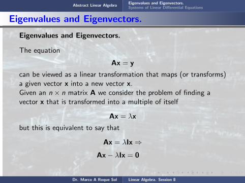
The equation
Ax = y
can be viewed as a linear transformation that maps (or transforms)a given vector x into a new vector x.Given an n × n matrix A we consider the problem of finding avector x that is transformed into a multiple of itself
Ax = λx
but this is equivalent to say that
Ax = λIx⇒
Ax− λIx = 0⇒
(A− λI) x = 0
Dr. Marco A Roque Sol Linear Algebra. Session 8

Abstract Linear AlgebraEigenvalues and Eigenvectors.Systems of Linear Differential Equations
Eigenvalues and Eigenvectors.
Eigenvalues and Eigenvectors.
The equation
Ax = y
can be viewed as a linear transformation that maps (or transforms)a given vector x into a new vector x.Given an n × n matrix A we consider the problem of finding avector x that is transformed into a multiple of itself
Ax = λx
but this is equivalent to say that
Ax = λIx⇒
Ax− λIx = 0⇒
(A− λI) x = 0
Dr. Marco A Roque Sol Linear Algebra. Session 8
Abstract Linear AlgebraEigenvalues and Eigenvectors.Systems of Linear Differential Equations
Eigenvalues and Eigenvectors.
Eigenvalues and Eigenvectors.
The equation
Ax = y
can be viewed
as a linear transformation that maps (or transforms)a given vector x into a new vector x.Given an n × n matrix A we consider the problem of finding avector x that is transformed into a multiple of itself
Ax = λx
but this is equivalent to say that
Ax = λIx⇒
Ax− λIx = 0⇒
(A− λI) x = 0
Dr. Marco A Roque Sol Linear Algebra. Session 8
Abstract Linear AlgebraEigenvalues and Eigenvectors.Systems of Linear Differential Equations
Eigenvalues and Eigenvectors.
Eigenvalues and Eigenvectors.
The equation
Ax = y
can be viewed as a linear transformation
that maps (or transforms)a given vector x into a new vector x.Given an n × n matrix A we consider the problem of finding avector x that is transformed into a multiple of itself
Ax = λx
but this is equivalent to say that
Ax = λIx⇒
Ax− λIx = 0⇒
(A− λI) x = 0
Dr. Marco A Roque Sol Linear Algebra. Session 8

Abstract Linear AlgebraEigenvalues and Eigenvectors.Systems of Linear Differential Equations
Eigenvalues and Eigenvectors.
Eigenvalues and Eigenvectors.
The equation
Ax = y
can be viewed as a linear transformation that maps
(or transforms)a given vector x into a new vector x.Given an n × n matrix A we consider the problem of finding avector x that is transformed into a multiple of itself
Ax = λx
but this is equivalent to say that
Ax = λIx⇒
Ax− λIx = 0⇒
(A− λI) x = 0
Dr. Marco A Roque Sol Linear Algebra. Session 8

Abstract Linear AlgebraEigenvalues and Eigenvectors.Systems of Linear Differential Equations
Eigenvalues and Eigenvectors.
Eigenvalues and Eigenvectors.
The equation
Ax = y
can be viewed as a linear transformation that maps (or transforms)
a given vector x into a new vector x.Given an n × n matrix A we consider the problem of finding avector x that is transformed into a multiple of itself
Ax = λx
but this is equivalent to say that
Ax = λIx⇒
Ax− λIx = 0⇒
(A− λI) x = 0
Dr. Marco A Roque Sol Linear Algebra. Session 8

Abstract Linear AlgebraEigenvalues and Eigenvectors.Systems of Linear Differential Equations
Eigenvalues and Eigenvectors.
Eigenvalues and Eigenvectors.
The equation
Ax = y
can be viewed as a linear transformation that maps (or transforms)a given vector
x into a new vector x.Given an n × n matrix A we consider the problem of finding avector x that is transformed into a multiple of itself
Ax = λx
but this is equivalent to say that
Ax = λIx⇒
Ax− λIx = 0⇒
(A− λI) x = 0
Dr. Marco A Roque Sol Linear Algebra. Session 8

Abstract Linear AlgebraEigenvalues and Eigenvectors.Systems of Linear Differential Equations
Eigenvalues and Eigenvectors.
Eigenvalues and Eigenvectors.
The equation
Ax = y
can be viewed as a linear transformation that maps (or transforms)a given vector x
into a new vector x.Given an n × n matrix A we consider the problem of finding avector x that is transformed into a multiple of itself
Ax = λx
but this is equivalent to say that
Ax = λIx⇒
Ax− λIx = 0⇒
(A− λI) x = 0
Dr. Marco A Roque Sol Linear Algebra. Session 8

Abstract Linear AlgebraEigenvalues and Eigenvectors.Systems of Linear Differential Equations
Eigenvalues and Eigenvectors.
Eigenvalues and Eigenvectors.
The equation
Ax = y
can be viewed as a linear transformation that maps (or transforms)a given vector x into
a new vector x.Given an n × n matrix A we consider the problem of finding avector x that is transformed into a multiple of itself
Ax = λx
but this is equivalent to say that
Ax = λIx⇒
Ax− λIx = 0⇒
(A− λI) x = 0
Dr. Marco A Roque Sol Linear Algebra. Session 8
Abstract Linear AlgebraEigenvalues and Eigenvectors.Systems of Linear Differential Equations
Eigenvalues and Eigenvectors.
Eigenvalues and Eigenvectors.
The equation
Ax = y
can be viewed as a linear transformation that maps (or transforms)a given vector x into a new vector x.Given
an n × n matrix A we consider the problem of finding avector x that is transformed into a multiple of itself
Ax = λx
but this is equivalent to say that
Ax = λIx⇒
Ax− λIx = 0⇒
(A− λI) x = 0
Dr. Marco A Roque Sol Linear Algebra. Session 8
Abstract Linear AlgebraEigenvalues and Eigenvectors.Systems of Linear Differential Equations
Eigenvalues and Eigenvectors.
Eigenvalues and Eigenvectors.
The equation
Ax = y
can be viewed as a linear transformation that maps (or transforms)a given vector x into a new vector x.Given an n × n matrix
A we consider the problem of finding avector x that is transformed into a multiple of itself
Ax = λx
but this is equivalent to say that
Ax = λIx⇒
Ax− λIx = 0⇒
(A− λI) x = 0
Dr. Marco A Roque Sol Linear Algebra. Session 8

Abstract Linear AlgebraEigenvalues and Eigenvectors.Systems of Linear Differential Equations
Eigenvalues and Eigenvectors.
Eigenvalues and Eigenvectors.
The equation
Ax = y
can be viewed as a linear transformation that maps (or transforms)a given vector x into a new vector x.Given an n × n matrix A
we consider the problem of finding avector x that is transformed into a multiple of itself
Ax = λx
but this is equivalent to say that
Ax = λIx⇒
Ax− λIx = 0⇒
(A− λI) x = 0
Dr. Marco A Roque Sol Linear Algebra. Session 8

Abstract Linear AlgebraEigenvalues and Eigenvectors.Systems of Linear Differential Equations
Eigenvalues and Eigenvectors.
Eigenvalues and Eigenvectors.
The equation
Ax = y
can be viewed as a linear transformation that maps (or transforms)a given vector x into a new vector x.Given an n × n matrix A we consider
the problem of finding avector x that is transformed into a multiple of itself
Ax = λx
but this is equivalent to say that
Ax = λIx⇒
Ax− λIx = 0⇒
(A− λI) x = 0
Dr. Marco A Roque Sol Linear Algebra. Session 8

Abstract Linear AlgebraEigenvalues and Eigenvectors.Systems of Linear Differential Equations
Eigenvalues and Eigenvectors.
Eigenvalues and Eigenvectors.
The equation
Ax = y
can be viewed as a linear transformation that maps (or transforms)a given vector x into a new vector x.Given an n × n matrix A we consider the problem
of finding avector x that is transformed into a multiple of itself
Ax = λx
but this is equivalent to say that
Ax = λIx⇒
Ax− λIx = 0⇒
(A− λI) x = 0
Dr. Marco A Roque Sol Linear Algebra. Session 8

Abstract Linear AlgebraEigenvalues and Eigenvectors.Systems of Linear Differential Equations
Eigenvalues and Eigenvectors.
Eigenvalues and Eigenvectors.
The equation
Ax = y
can be viewed as a linear transformation that maps (or transforms)a given vector x into a new vector x.Given an n × n matrix A we consider the problem of finding
avector x that is transformed into a multiple of itself
Ax = λx
but this is equivalent to say that
Ax = λIx⇒
Ax− λIx = 0⇒
(A− λI) x = 0
Dr. Marco A Roque Sol Linear Algebra. Session 8

Abstract Linear AlgebraEigenvalues and Eigenvectors.Systems of Linear Differential Equations
Eigenvalues and Eigenvectors.
Eigenvalues and Eigenvectors.
The equation
Ax = y
can be viewed as a linear transformation that maps (or transforms)a given vector x into a new vector x.Given an n × n matrix A we consider the problem of finding avector x
that is transformed into a multiple of itself
Ax = λx
but this is equivalent to say that
Ax = λIx⇒
Ax− λIx = 0⇒
(A− λI) x = 0
Dr. Marco A Roque Sol Linear Algebra. Session 8
Abstract Linear AlgebraEigenvalues and Eigenvectors.Systems of Linear Differential Equations
Eigenvalues and Eigenvectors.
Eigenvalues and Eigenvectors.
The equation
Ax = y
can be viewed as a linear transformation that maps (or transforms)a given vector x into a new vector x.Given an n × n matrix A we consider the problem of finding avector x that is transformed
into a multiple of itself
Ax = λx
but this is equivalent to say that
Ax = λIx⇒
Ax− λIx = 0⇒
(A− λI) x = 0
Dr. Marco A Roque Sol Linear Algebra. Session 8

Abstract Linear AlgebraEigenvalues and Eigenvectors.Systems of Linear Differential Equations
Eigenvalues and Eigenvectors.
Eigenvalues and Eigenvectors.
The equation
Ax = y
can be viewed as a linear transformation that maps (or transforms)a given vector x into a new vector x.Given an n × n matrix A we consider the problem of finding avector x that is transformed into a multiple
of itself
Ax = λx
but this is equivalent to say that
Ax = λIx⇒
Ax− λIx = 0⇒
(A− λI) x = 0
Dr. Marco A Roque Sol Linear Algebra. Session 8

Abstract Linear AlgebraEigenvalues and Eigenvectors.Systems of Linear Differential Equations
Eigenvalues and Eigenvectors.
Eigenvalues and Eigenvectors.
The equation
Ax = y
can be viewed as a linear transformation that maps (or transforms)a given vector x into a new vector x.Given an n × n matrix A we consider the problem of finding avector x that is transformed into a multiple of itself
Ax = λx
but this is equivalent to say that
Ax = λIx⇒
Ax− λIx = 0⇒
(A− λI) x = 0
Dr. Marco A Roque Sol Linear Algebra. Session 8
Abstract Linear AlgebraEigenvalues and Eigenvectors.Systems of Linear Differential Equations
Eigenvalues and Eigenvectors.
Eigenvalues and Eigenvectors.
The equation
Ax = y
can be viewed as a linear transformation that maps (or transforms)a given vector x into a new vector x.Given an n × n matrix A we consider the problem of finding avector x that is transformed into a multiple of itself
Ax = λx
but
this is equivalent to say that
Ax = λIx⇒
Ax− λIx = 0⇒
(A− λI) x = 0
Dr. Marco A Roque Sol Linear Algebra. Session 8

Abstract Linear AlgebraEigenvalues and Eigenvectors.Systems of Linear Differential Equations
Eigenvalues and Eigenvectors.
Eigenvalues and Eigenvectors.
The equation
Ax = y
can be viewed as a linear transformation that maps (or transforms)a given vector x into a new vector x.Given an n × n matrix A we consider the problem of finding avector x that is transformed into a multiple of itself
Ax = λx
but this is equivalent
to say that
Ax = λIx⇒
Ax− λIx = 0⇒
(A− λI) x = 0
Dr. Marco A Roque Sol Linear Algebra. Session 8

Abstract Linear AlgebraEigenvalues and Eigenvectors.Systems of Linear Differential Equations
Eigenvalues and Eigenvectors.
Eigenvalues and Eigenvectors.
The equation
Ax = y
can be viewed as a linear transformation that maps (or transforms)a given vector x into a new vector x.Given an n × n matrix A we consider the problem of finding avector x that is transformed into a multiple of itself
Ax = λx
but this is equivalent to say that
Ax = λIx⇒
Ax− λIx = 0⇒
(A− λI) x = 0
Dr. Marco A Roque Sol Linear Algebra. Session 8

Abstract Linear AlgebraEigenvalues and Eigenvectors.Systems of Linear Differential Equations
Eigenvalues and Eigenvectors.
Eigenvalues and Eigenvectors.
The equation
Ax = y
can be viewed as a linear transformation that maps (or transforms)a given vector x into a new vector x.Given an n × n matrix A we consider the problem of finding avector x that is transformed into a multiple of itself
Ax = λx
but this is equivalent to say that
Ax = λIx
⇒
Ax− λIx = 0⇒
(A− λI) x = 0
Dr. Marco A Roque Sol Linear Algebra. Session 8
Abstract Linear AlgebraEigenvalues and Eigenvectors.Systems of Linear Differential Equations
Eigenvalues and Eigenvectors.
Eigenvalues and Eigenvectors.
The equation
Ax = y
can be viewed as a linear transformation that maps (or transforms)a given vector x into a new vector x.Given an n × n matrix A we consider the problem of finding avector x that is transformed into a multiple of itself
Ax = λx
but this is equivalent to say that
Ax = λIx⇒
Ax− λIx = 0⇒
(A− λI) x = 0
Dr. Marco A Roque Sol Linear Algebra. Session 8
Abstract Linear AlgebraEigenvalues and Eigenvectors.Systems of Linear Differential Equations
Eigenvalues and Eigenvectors.
Eigenvalues and Eigenvectors.
The equation
Ax = y
can be viewed as a linear transformation that maps (or transforms)a given vector x into a new vector x.Given an n × n matrix A we consider the problem of finding avector x that is transformed into a multiple of itself
Ax = λx
but this is equivalent to say that
Ax = λIx⇒
Ax− λIx = 0
⇒
(A− λI) x = 0
Dr. Marco A Roque Sol Linear Algebra. Session 8

Abstract Linear AlgebraEigenvalues and Eigenvectors.Systems of Linear Differential Equations
Eigenvalues and Eigenvectors.
Eigenvalues and Eigenvectors.
The equation
Ax = y
can be viewed as a linear transformation that maps (or transforms)a given vector x into a new vector x.Given an n × n matrix A we consider the problem of finding avector x that is transformed into a multiple of itself
Ax = λx
but this is equivalent to say that
Ax = λIx⇒
Ax− λIx = 0⇒
(A− λI) x = 0
Dr. Marco A Roque Sol Linear Algebra. Session 8

Abstract Linear AlgebraEigenvalues and Eigenvectors.Systems of Linear Differential Equations
Eigenvalues and Eigenvectors.
Eigenvalues and Eigenvectors.
The equation
Ax = y
can be viewed as a linear transformation that maps (or transforms)a given vector x into a new vector x.Given an n × n matrix A we consider the problem of finding avector x that is transformed into a multiple of itself
Ax = λx
but this is equivalent to say that
Ax = λIx⇒
Ax− λIx = 0⇒
(A− λI) x = 0Dr. Marco A Roque Sol Linear Algebra. Session 8

Abstract Linear AlgebraEigenvalues and Eigenvectors.Systems of Linear Differential Equations
Eigenvalues and Eigenvectors.
The latter equation has nonzero solutions if and only if λ is chosenso that
|A− λI| = 0
This is a polynomial equation of degree n in λ and is called thecharacteristic equation of the matrix A
Values of λ may be either real or complex-valued and are calledeigenvalues of A . The nonzero vectors that are obtained by usingsuch a value of λ are called the eigenvectors corresponding tothat eigenvalue.
Dr. Marco A Roque Sol Linear Algebra. Session 8

Abstract Linear AlgebraEigenvalues and Eigenvectors.Systems of Linear Differential Equations
Eigenvalues and Eigenvectors.
The latter equation
has nonzero solutions if and only if λ is chosenso that
|A− λI| = 0
This is a polynomial equation of degree n in λ and is called thecharacteristic equation of the matrix A
Values of λ may be either real or complex-valued and are calledeigenvalues of A . The nonzero vectors that are obtained by usingsuch a value of λ are called the eigenvectors corresponding tothat eigenvalue.
Dr. Marco A Roque Sol Linear Algebra. Session 8

Abstract Linear AlgebraEigenvalues and Eigenvectors.Systems of Linear Differential Equations
Eigenvalues and Eigenvectors.
The latter equation has nonzero solutions
if and only if λ is chosenso that
|A− λI| = 0
This is a polynomial equation of degree n in λ and is called thecharacteristic equation of the matrix A
Values of λ may be either real or complex-valued and are calledeigenvalues of A . The nonzero vectors that are obtained by usingsuch a value of λ are called the eigenvectors corresponding tothat eigenvalue.
Dr. Marco A Roque Sol Linear Algebra. Session 8

Abstract Linear AlgebraEigenvalues and Eigenvectors.Systems of Linear Differential Equations
Eigenvalues and Eigenvectors.
The latter equation has nonzero solutions if and only if
λ is chosenso that
|A− λI| = 0
This is a polynomial equation of degree n in λ and is called thecharacteristic equation of the matrix A
Values of λ may be either real or complex-valued and are calledeigenvalues of A . The nonzero vectors that are obtained by usingsuch a value of λ are called the eigenvectors corresponding tothat eigenvalue.
Dr. Marco A Roque Sol Linear Algebra. Session 8
Abstract Linear AlgebraEigenvalues and Eigenvectors.Systems of Linear Differential Equations
Eigenvalues and Eigenvectors.
The latter equation has nonzero solutions if and only if λ
is chosenso that
|A− λI| = 0
This is a polynomial equation of degree n in λ and is called thecharacteristic equation of the matrix A
Values of λ may be either real or complex-valued and are calledeigenvalues of A . The nonzero vectors that are obtained by usingsuch a value of λ are called the eigenvectors corresponding tothat eigenvalue.
Dr. Marco A Roque Sol Linear Algebra. Session 8

Abstract Linear AlgebraEigenvalues and Eigenvectors.Systems of Linear Differential Equations
Eigenvalues and Eigenvectors.
The latter equation has nonzero solutions if and only if λ is chosenso
that
|A− λI| = 0
This is a polynomial equation of degree n in λ and is called thecharacteristic equation of the matrix A
Values of λ may be either real or complex-valued and are calledeigenvalues of A . The nonzero vectors that are obtained by usingsuch a value of λ are called the eigenvectors corresponding tothat eigenvalue.
Dr. Marco A Roque Sol Linear Algebra. Session 8

Abstract Linear AlgebraEigenvalues and Eigenvectors.Systems of Linear Differential Equations
Eigenvalues and Eigenvectors.
The latter equation has nonzero solutions if and only if λ is chosenso that
|A− λI| = 0
This is a polynomial equation of degree n in λ and is called thecharacteristic equation of the matrix A
Values of λ may be either real or complex-valued and are calledeigenvalues of A . The nonzero vectors that are obtained by usingsuch a value of λ are called the eigenvectors corresponding tothat eigenvalue.
Dr. Marco A Roque Sol Linear Algebra. Session 8

Abstract Linear AlgebraEigenvalues and Eigenvectors.Systems of Linear Differential Equations
Eigenvalues and Eigenvectors.
The latter equation has nonzero solutions if and only if λ is chosenso that
|A− λI| = 0
This is a polynomial equation of degree n in λ and is called thecharacteristic equation of the matrix A
Values of λ may be either real or complex-valued and are calledeigenvalues of A . The nonzero vectors that are obtained by usingsuch a value of λ are called the eigenvectors corresponding tothat eigenvalue.
Dr. Marco A Roque Sol Linear Algebra. Session 8
Abstract Linear AlgebraEigenvalues and Eigenvectors.Systems of Linear Differential Equations
Eigenvalues and Eigenvectors.
The latter equation has nonzero solutions if and only if λ is chosenso that
|A− λI| = 0
This is
a polynomial equation of degree n in λ and is called thecharacteristic equation of the matrix A
Values of λ may be either real or complex-valued and are calledeigenvalues of A . The nonzero vectors that are obtained by usingsuch a value of λ are called the eigenvectors corresponding tothat eigenvalue.
Dr. Marco A Roque Sol Linear Algebra. Session 8

Abstract Linear AlgebraEigenvalues and Eigenvectors.Systems of Linear Differential Equations
Eigenvalues and Eigenvectors.
The latter equation has nonzero solutions if and only if λ is chosenso that
|A− λI| = 0
This is a polynomial equation
of degree n in λ and is called thecharacteristic equation of the matrix A
Values of λ may be either real or complex-valued and are calledeigenvalues of A . The nonzero vectors that are obtained by usingsuch a value of λ are called the eigenvectors corresponding tothat eigenvalue.
Dr. Marco A Roque Sol Linear Algebra. Session 8

Abstract Linear AlgebraEigenvalues and Eigenvectors.Systems of Linear Differential Equations
Eigenvalues and Eigenvectors.
The latter equation has nonzero solutions if and only if λ is chosenso that
|A− λI| = 0
This is a polynomial equation of degree n
in λ and is called thecharacteristic equation of the matrix A
Values of λ may be either real or complex-valued and are calledeigenvalues of A . The nonzero vectors that are obtained by usingsuch a value of λ are called the eigenvectors corresponding tothat eigenvalue.
Dr. Marco A Roque Sol Linear Algebra. Session 8

Abstract Linear AlgebraEigenvalues and Eigenvectors.Systems of Linear Differential Equations
Eigenvalues and Eigenvectors.
The latter equation has nonzero solutions if and only if λ is chosenso that
|A− λI| = 0
This is a polynomial equation of degree n in λ
and is called thecharacteristic equation of the matrix A
Values of λ may be either real or complex-valued and are calledeigenvalues of A . The nonzero vectors that are obtained by usingsuch a value of λ are called the eigenvectors corresponding tothat eigenvalue.
Dr. Marco A Roque Sol Linear Algebra. Session 8
Abstract Linear AlgebraEigenvalues and Eigenvectors.Systems of Linear Differential Equations
Eigenvalues and Eigenvectors.
The latter equation has nonzero solutions if and only if λ is chosenso that
|A− λI| = 0
This is a polynomial equation of degree n in λ and is called
thecharacteristic equation of the matrix A
Values of λ may be either real or complex-valued and are calledeigenvalues of A . The nonzero vectors that are obtained by usingsuch a value of λ are called the eigenvectors corresponding tothat eigenvalue.
Dr. Marco A Roque Sol Linear Algebra. Session 8

Abstract Linear AlgebraEigenvalues and Eigenvectors.Systems of Linear Differential Equations
Eigenvalues and Eigenvectors.
The latter equation has nonzero solutions if and only if λ is chosenso that
|A− λI| = 0
This is a polynomial equation of degree n in λ and is called thecharacteristic equation
of the matrix A
Values of λ may be either real or complex-valued and are calledeigenvalues of A . The nonzero vectors that are obtained by usingsuch a value of λ are called the eigenvectors corresponding tothat eigenvalue.
Dr. Marco A Roque Sol Linear Algebra. Session 8

Abstract Linear AlgebraEigenvalues and Eigenvectors.Systems of Linear Differential Equations
Eigenvalues and Eigenvectors.
The latter equation has nonzero solutions if and only if λ is chosenso that
|A− λI| = 0
This is a polynomial equation of degree n in λ and is called thecharacteristic equation of the matrix A
Values of λ may be either real or complex-valued and are calledeigenvalues of A . The nonzero vectors that are obtained by usingsuch a value of λ are called the eigenvectors corresponding tothat eigenvalue.
Dr. Marco A Roque Sol Linear Algebra. Session 8
Abstract Linear AlgebraEigenvalues and Eigenvectors.Systems of Linear Differential Equations
Eigenvalues and Eigenvectors.
The latter equation has nonzero solutions if and only if λ is chosenso that
|A− λI| = 0
This is a polynomial equation of degree n in λ and is called thecharacteristic equation of the matrix A
Values of λ
may be either real or complex-valued and are calledeigenvalues of A . The nonzero vectors that are obtained by usingsuch a value of λ are called the eigenvectors corresponding tothat eigenvalue.
Dr. Marco A Roque Sol Linear Algebra. Session 8
Abstract Linear AlgebraEigenvalues and Eigenvectors.Systems of Linear Differential Equations
Eigenvalues and Eigenvectors.
The latter equation has nonzero solutions if and only if λ is chosenso that
|A− λI| = 0
This is a polynomial equation of degree n in λ and is called thecharacteristic equation of the matrix A
Values of λ may be either real or complex-valued and
are calledeigenvalues of A . The nonzero vectors that are obtained by usingsuch a value of λ are called the eigenvectors corresponding tothat eigenvalue.
Dr. Marco A Roque Sol Linear Algebra. Session 8

Abstract Linear AlgebraEigenvalues and Eigenvectors.Systems of Linear Differential Equations
Eigenvalues and Eigenvectors.
The latter equation has nonzero solutions if and only if λ is chosenso that
|A− λI| = 0
This is a polynomial equation of degree n in λ and is called thecharacteristic equation of the matrix A
Values of λ may be either real or complex-valued and are called
eigenvalues of A . The nonzero vectors that are obtained by usingsuch a value of λ are called the eigenvectors corresponding tothat eigenvalue.
Dr. Marco A Roque Sol Linear Algebra. Session 8
Abstract Linear AlgebraEigenvalues and Eigenvectors.Systems of Linear Differential Equations
Eigenvalues and Eigenvectors.
The latter equation has nonzero solutions if and only if λ is chosenso that
|A− λI| = 0
This is a polynomial equation of degree n in λ and is called thecharacteristic equation of the matrix A
Values of λ may be either real or complex-valued and are calledeigenvalues
of A . The nonzero vectors that are obtained by usingsuch a value of λ are called the eigenvectors corresponding tothat eigenvalue.
Dr. Marco A Roque Sol Linear Algebra. Session 8
Abstract Linear AlgebraEigenvalues and Eigenvectors.Systems of Linear Differential Equations
Eigenvalues and Eigenvectors.
The latter equation has nonzero solutions if and only if λ is chosenso that
|A− λI| = 0
This is a polynomial equation of degree n in λ and is called thecharacteristic equation of the matrix A
Values of λ may be either real or complex-valued and are calledeigenvalues of A .
The nonzero vectors that are obtained by usingsuch a value of λ are called the eigenvectors corresponding tothat eigenvalue.
Dr. Marco A Roque Sol Linear Algebra. Session 8
Abstract Linear AlgebraEigenvalues and Eigenvectors.Systems of Linear Differential Equations
Eigenvalues and Eigenvectors.
The latter equation has nonzero solutions if and only if λ is chosenso that
|A− λI| = 0
This is a polynomial equation of degree n in λ and is called thecharacteristic equation of the matrix A
Values of λ may be either real or complex-valued and are calledeigenvalues of A . The nonzero vectors
that are obtained by usingsuch a value of λ are called the eigenvectors corresponding tothat eigenvalue.
Dr. Marco A Roque Sol Linear Algebra. Session 8

Abstract Linear AlgebraEigenvalues and Eigenvectors.Systems of Linear Differential Equations
Eigenvalues and Eigenvectors.
The latter equation has nonzero solutions if and only if λ is chosenso that
|A− λI| = 0
This is a polynomial equation of degree n in λ and is called thecharacteristic equation of the matrix A
Values of λ may be either real or complex-valued and are calledeigenvalues of A . The nonzero vectors that are obtained
by usingsuch a value of λ are called the eigenvectors corresponding tothat eigenvalue.
Dr. Marco A Roque Sol Linear Algebra. Session 8
Abstract Linear AlgebraEigenvalues and Eigenvectors.Systems of Linear Differential Equations
Eigenvalues and Eigenvectors.
The latter equation has nonzero solutions if and only if λ is chosenso that
|A− λI| = 0
This is a polynomial equation of degree n in λ and is called thecharacteristic equation of the matrix A
Values of λ may be either real or complex-valued and are calledeigenvalues of A . The nonzero vectors that are obtained by using
such a value of λ are called the eigenvectors corresponding tothat eigenvalue.
Dr. Marco A Roque Sol Linear Algebra. Session 8
Abstract Linear AlgebraEigenvalues and Eigenvectors.Systems of Linear Differential Equations
Eigenvalues and Eigenvectors.
The latter equation has nonzero solutions if and only if λ is chosenso that
|A− λI| = 0
This is a polynomial equation of degree n in λ and is called thecharacteristic equation of the matrix A
Values of λ may be either real or complex-valued and are calledeigenvalues of A . The nonzero vectors that are obtained by usingsuch a value
of λ are called the eigenvectors corresponding tothat eigenvalue.
Dr. Marco A Roque Sol Linear Algebra. Session 8
Abstract Linear AlgebraEigenvalues and Eigenvectors.Systems of Linear Differential Equations
Eigenvalues and Eigenvectors.
The latter equation has nonzero solutions if and only if λ is chosenso that
|A− λI| = 0
This is a polynomial equation of degree n in λ and is called thecharacteristic equation of the matrix A
Values of λ may be either real or complex-valued and are calledeigenvalues of A . The nonzero vectors that are obtained by usingsuch a value of λ
are called the eigenvectors corresponding tothat eigenvalue.
Dr. Marco A Roque Sol Linear Algebra. Session 8

Abstract Linear AlgebraEigenvalues and Eigenvectors.Systems of Linear Differential Equations
Eigenvalues and Eigenvectors.
The latter equation has nonzero solutions if and only if λ is chosenso that
|A− λI| = 0
This is a polynomial equation of degree n in λ and is called thecharacteristic equation of the matrix A
Values of λ may be either real or complex-valued and are calledeigenvalues of A . The nonzero vectors that are obtained by usingsuch a value of λ are called
the eigenvectors corresponding tothat eigenvalue.
Dr. Marco A Roque Sol Linear Algebra. Session 8
Abstract Linear AlgebraEigenvalues and Eigenvectors.Systems of Linear Differential Equations
Eigenvalues and Eigenvectors.
The latter equation has nonzero solutions if and only if λ is chosenso that
|A− λI| = 0
This is a polynomial equation of degree n in λ and is called thecharacteristic equation of the matrix A
Values of λ may be either real or complex-valued and are calledeigenvalues of A . The nonzero vectors that are obtained by usingsuch a value of λ are called the eigenvectors
corresponding tothat eigenvalue.
Dr. Marco A Roque Sol Linear Algebra. Session 8
Abstract Linear AlgebraEigenvalues and Eigenvectors.Systems of Linear Differential Equations
Eigenvalues and Eigenvectors.
The latter equation has nonzero solutions if and only if λ is chosenso that
|A− λI| = 0
This is a polynomial equation of degree n in λ and is called thecharacteristic equation of the matrix A
Values of λ may be either real or complex-valued and are calledeigenvalues of A . The nonzero vectors that are obtained by usingsuch a value of λ are called the eigenvectors corresponding
tothat eigenvalue.
Dr. Marco A Roque Sol Linear Algebra. Session 8

Abstract Linear AlgebraEigenvalues and Eigenvectors.Systems of Linear Differential Equations
Eigenvalues and Eigenvectors.
The latter equation has nonzero solutions if and only if λ is chosenso that
|A− λI| = 0
This is a polynomial equation of degree n in λ and is called thecharacteristic equation of the matrix A
Values of λ may be either real or complex-valued and are calledeigenvalues of A . The nonzero vectors that are obtained by usingsuch a value of λ are called the eigenvectors corresponding tothat eigenvalue.
Dr. Marco A Roque Sol Linear Algebra. Session 8

Abstract Linear AlgebraEigenvalues and Eigenvectors.Systems of Linear Differential Equations
Eigenvalues and Eigenvectors.
Facts
a) It is possible to show that if λ1 and λ2 are two eigenvalues of Aandif λ1 6= λ2, then their corresponding eigenvectors x (1) and x (2)
are linearly independent.
This result extends to any set λ1, ..., λk of distinct eigenvalues:their eigenvectors x (1), ..., x (k) are linearly independent. Thus, ifeach eigenvalue of an n×n matrix is simple,then the n eigenvectorsof A , one for each eigenvalue, are linearly independent.
Dr. Marco A Roque Sol Linear Algebra. Session 8

Abstract Linear AlgebraEigenvalues and Eigenvectors.Systems of Linear Differential Equations
Eigenvalues and Eigenvectors.
Facts
a) It is possible to show that if λ1 and λ2
are two eigenvalues of Aandif λ1 6= λ2, then their corresponding eigenvectors x (1) and x (2)
are linearly independent.
This result extends to any set λ1, ..., λk of distinct eigenvalues:their eigenvectors x (1), ..., x (k) are linearly independent. Thus, ifeach eigenvalue of an n×n matrix is simple,then the n eigenvectorsof A , one for each eigenvalue, are linearly independent.
Dr. Marco A Roque Sol Linear Algebra. Session 8

Abstract Linear AlgebraEigenvalues and Eigenvectors.Systems of Linear Differential Equations
Eigenvalues and Eigenvectors.
Facts
a) It is possible to show that if λ1 and λ2 are two eigenvalues of Aand
if λ1 6= λ2, then their corresponding eigenvectors x (1) and x (2)
are linearly independent.
This result extends to any set λ1, ..., λk of distinct eigenvalues:their eigenvectors x (1), ..., x (k) are linearly independent. Thus, ifeach eigenvalue of an n×n matrix is simple,then the n eigenvectorsof A , one for each eigenvalue, are linearly independent.
Dr. Marco A Roque Sol Linear Algebra. Session 8
Abstract Linear AlgebraEigenvalues and Eigenvectors.Systems of Linear Differential Equations
Eigenvalues and Eigenvectors.
Facts
a) It is possible to show that if λ1 and λ2 are two eigenvalues of Aandif λ1 6= λ2, then
their corresponding eigenvectors x (1) and x (2)
are linearly independent.
This result extends to any set λ1, ..., λk of distinct eigenvalues:their eigenvectors x (1), ..., x (k) are linearly independent. Thus, ifeach eigenvalue of an n×n matrix is simple,then the n eigenvectorsof A , one for each eigenvalue, are linearly independent.
Dr. Marco A Roque Sol Linear Algebra. Session 8
Abstract Linear AlgebraEigenvalues and Eigenvectors.Systems of Linear Differential Equations
Eigenvalues and Eigenvectors.
Facts
a) It is possible to show that if λ1 and λ2 are two eigenvalues of Aandif λ1 6= λ2, then their corresponding eigenvectors x (1) and x (2)
are linearly independent.
This result extends to any set λ1, ..., λk of distinct eigenvalues:their eigenvectors x (1), ..., x (k) are linearly independent. Thus, ifeach eigenvalue of an n×n matrix is simple,then the n eigenvectorsof A , one for each eigenvalue, are linearly independent.
Dr. Marco A Roque Sol Linear Algebra. Session 8
Abstract Linear AlgebraEigenvalues and Eigenvectors.Systems of Linear Differential Equations
Eigenvalues and Eigenvectors.
Facts
a) It is possible to show that if λ1 and λ2 are two eigenvalues of Aandif λ1 6= λ2, then their corresponding eigenvectors x (1) and x (2)
are linearly independent.
This result extends to any set λ1, ..., λk of distinct eigenvalues:
their eigenvectors x (1), ..., x (k) are linearly independent. Thus, ifeach eigenvalue of an n×n matrix is simple,then the n eigenvectorsof A , one for each eigenvalue, are linearly independent.
Dr. Marco A Roque Sol Linear Algebra. Session 8

Abstract Linear AlgebraEigenvalues and Eigenvectors.Systems of Linear Differential Equations
Eigenvalues and Eigenvectors.
Facts
a) It is possible to show that if λ1 and λ2 are two eigenvalues of Aandif λ1 6= λ2, then their corresponding eigenvectors x (1) and x (2)
are linearly independent.
This result extends to any set λ1, ..., λk of distinct eigenvalues:their eigenvectors x (1), ..., x (k) are linearly independent.
Thus, ifeach eigenvalue of an n×n matrix is simple,then the n eigenvectorsof A , one for each eigenvalue, are linearly independent.
Dr. Marco A Roque Sol Linear Algebra. Session 8

Abstract Linear AlgebraEigenvalues and Eigenvectors.Systems of Linear Differential Equations
Eigenvalues and Eigenvectors.
Facts
a) It is possible to show that if λ1 and λ2 are two eigenvalues of Aandif λ1 6= λ2, then their corresponding eigenvectors x (1) and x (2)
are linearly independent.
This result extends to any set λ1, ..., λk of distinct eigenvalues:their eigenvectors x (1), ..., x (k) are linearly independent. Thus, ifeach eigenvalue of an n×n matrix is simple,
then the n eigenvectorsof A , one for each eigenvalue, are linearly independent.
Dr. Marco A Roque Sol Linear Algebra. Session 8

Abstract Linear AlgebraEigenvalues and Eigenvectors.Systems of Linear Differential Equations
Eigenvalues and Eigenvectors.
Facts
a) It is possible to show that if λ1 and λ2 are two eigenvalues of Aandif λ1 6= λ2, then their corresponding eigenvectors x (1) and x (2)
are linearly independent.
This result extends to any set λ1, ..., λk of distinct eigenvalues:their eigenvectors x (1), ..., x (k) are linearly independent. Thus, ifeach eigenvalue of an n×n matrix is simple,then the n eigenvectorsof A ,
one for each eigenvalue, are linearly independent.
Dr. Marco A Roque Sol Linear Algebra. Session 8

Abstract Linear AlgebraEigenvalues and Eigenvectors.Systems of Linear Differential Equations
Eigenvalues and Eigenvectors.
Facts
a) It is possible to show that if λ1 and λ2 are two eigenvalues of Aandif λ1 6= λ2, then their corresponding eigenvectors x (1) and x (2)
are linearly independent.
This result extends to any set λ1, ..., λk of distinct eigenvalues:their eigenvectors x (1), ..., x (k) are linearly independent. Thus, ifeach eigenvalue of an n×n matrix is simple,then the n eigenvectorsof A , one for each eigenvalue, are linearly independent.
Dr. Marco A Roque Sol Linear Algebra. Session 8

Abstract Linear AlgebraEigenvalues and Eigenvectors.Systems of Linear Differential Equations
Eigenvalues and Eigenvectors.
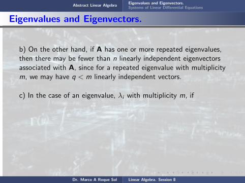
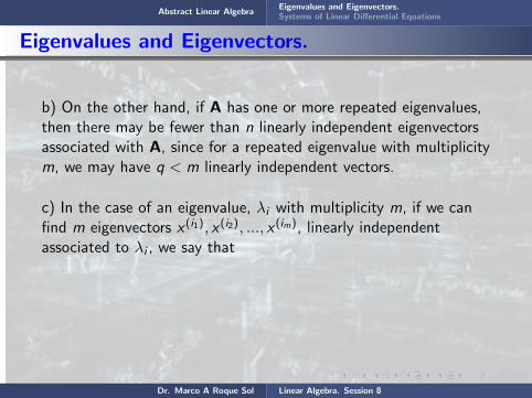
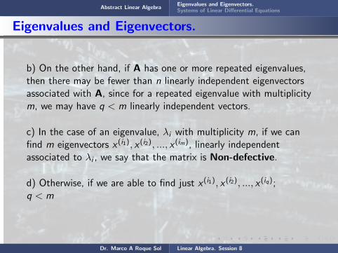
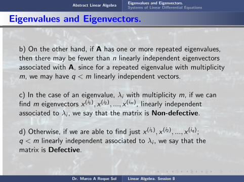
b) On the other hand, if A has one or more repeated eigenvalues,then there may be fewer than n linearly independent eigenvectorsassociated with A, since for a repeated eigenvalue with multiplicitym, we may have q < m linearly independent vectors.
c) In the case of an eigenvalue, λi with multiplicity m, if we canfind m eigenvectors x (i1), x (i2), ..., x (im), linearly independentassociated to λi , we say that the matrix is Non-defective.
d) Otherwise, if we are able to find just x (i1), x (i2), ..., x (iq);q < m linearly independent associated to λi , we say that thematrix is Defective.
Dr. Marco A Roque Sol Linear Algebra. Session 8

Abstract Linear AlgebraEigenvalues and Eigenvectors.Systems of Linear Differential Equations
Eigenvalues and Eigenvectors.
b) On the other hand,
if A has one or more repeated eigenvalues,then there may be fewer than n linearly independent eigenvectorsassociated with A, since for a repeated eigenvalue with multiplicitym, we may have q < m linearly independent vectors.
c) In the case of an eigenvalue, λi with multiplicity m, if we canfind m eigenvectors x (i1), x (i2), ..., x (im), linearly independentassociated to λi , we say that the matrix is Non-defective.
d) Otherwise, if we are able to find just x (i1), x (i2), ..., x (iq);q < m linearly independent associated to λi , we say that thematrix is Defective.
Dr. Marco A Roque Sol Linear Algebra. Session 8

Abstract Linear AlgebraEigenvalues and Eigenvectors.Systems of Linear Differential Equations
Eigenvalues and Eigenvectors.
b) On the other hand, if A
has one or more repeated eigenvalues,then there may be fewer than n linearly independent eigenvectorsassociated with A, since for a repeated eigenvalue with multiplicitym, we may have q < m linearly independent vectors.
c) In the case of an eigenvalue, λi with multiplicity m, if we canfind m eigenvectors x (i1), x (i2), ..., x (im), linearly independentassociated to λi , we say that the matrix is Non-defective.
d) Otherwise, if we are able to find just x (i1), x (i2), ..., x (iq);q < m linearly independent associated to λi , we say that thematrix is Defective.
Dr. Marco A Roque Sol Linear Algebra. Session 8
Abstract Linear AlgebraEigenvalues and Eigenvectors.Systems of Linear Differential Equations
Eigenvalues and Eigenvectors.
b) On the other hand, if A has one or more repeated eigenvalues,then
there may be fewer than n linearly independent eigenvectorsassociated with A, since for a repeated eigenvalue with multiplicitym, we may have q < m linearly independent vectors.
c) In the case of an eigenvalue, λi with multiplicity m, if we canfind m eigenvectors x (i1), x (i2), ..., x (im), linearly independentassociated to λi , we say that the matrix is Non-defective.
d) Otherwise, if we are able to find just x (i1), x (i2), ..., x (iq);q < m linearly independent associated to λi , we say that thematrix is Defective.
Dr. Marco A Roque Sol Linear Algebra. Session 8

Abstract Linear AlgebraEigenvalues and Eigenvectors.Systems of Linear Differential Equations
Eigenvalues and Eigenvectors.
b) On the other hand, if A has one or more repeated eigenvalues,then there may be
fewer than n linearly independent eigenvectorsassociated with A, since for a repeated eigenvalue with multiplicitym, we may have q < m linearly independent vectors.
c) In the case of an eigenvalue, λi with multiplicity m, if we canfind m eigenvectors x (i1), x (i2), ..., x (im), linearly independentassociated to λi , we say that the matrix is Non-defective.
d) Otherwise, if we are able to find just x (i1), x (i2), ..., x (iq);q < m linearly independent associated to λi , we say that thematrix is Defective.
Dr. Marco A Roque Sol Linear Algebra. Session 8

Abstract Linear AlgebraEigenvalues and Eigenvectors.Systems of Linear Differential Equations
Eigenvalues and Eigenvectors.
b) On the other hand, if A has one or more repeated eigenvalues,then there may be fewer than n linearly independent
eigenvectorsassociated with A, since for a repeated eigenvalue with multiplicitym, we may have q < m linearly independent vectors.
c) In the case of an eigenvalue, λi with multiplicity m, if we canfind m eigenvectors x (i1), x (i2), ..., x (im), linearly independentassociated to λi , we say that the matrix is Non-defective.
d) Otherwise, if we are able to find just x (i1), x (i2), ..., x (iq);q < m linearly independent associated to λi , we say that thematrix is Defective.
Dr. Marco A Roque Sol Linear Algebra. Session 8

Abstract Linear AlgebraEigenvalues and Eigenvectors.Systems of Linear Differential Equations
Eigenvalues and Eigenvectors.
b) On the other hand, if A has one or more repeated eigenvalues,then there may be fewer than n linearly independent eigenvectorsassociated
with A, since for a repeated eigenvalue with multiplicitym, we may have q < m linearly independent vectors.
c) In the case of an eigenvalue, λi with multiplicity m, if we canfind m eigenvectors x (i1), x (i2), ..., x (im), linearly independentassociated to λi , we say that the matrix is Non-defective.
d) Otherwise, if we are able to find just x (i1), x (i2), ..., x (iq);q < m linearly independent associated to λi , we say that thematrix is Defective.
Dr. Marco A Roque Sol Linear Algebra. Session 8

Abstract Linear AlgebraEigenvalues and Eigenvectors.Systems of Linear Differential Equations
Eigenvalues and Eigenvectors.
b) On the other hand, if A has one or more repeated eigenvalues,then there may be fewer than n linearly independent eigenvectorsassociated with A,
since for a repeated eigenvalue with multiplicitym, we may have q < m linearly independent vectors.
c) In the case of an eigenvalue, λi with multiplicity m, if we canfind m eigenvectors x (i1), x (i2), ..., x (im), linearly independentassociated to λi , we say that the matrix is Non-defective.
d) Otherwise, if we are able to find just x (i1), x (i2), ..., x (iq);q < m linearly independent associated to λi , we say that thematrix is Defective.
Dr. Marco A Roque Sol Linear Algebra. Session 8

Abstract Linear AlgebraEigenvalues and Eigenvectors.Systems of Linear Differential Equations
Eigenvalues and Eigenvectors.
b) On the other hand, if A has one or more repeated eigenvalues,then there may be fewer than n linearly independent eigenvectorsassociated with A, since for a repeated eigenvalue
with multiplicitym, we may have q < m linearly independent vectors.
c) In the case of an eigenvalue, λi with multiplicity m, if we canfind m eigenvectors x (i1), x (i2), ..., x (im), linearly independentassociated to λi , we say that the matrix is Non-defective.
d) Otherwise, if we are able to find just x (i1), x (i2), ..., x (iq);q < m linearly independent associated to λi , we say that thematrix is Defective.
Dr. Marco A Roque Sol Linear Algebra. Session 8
Abstract Linear AlgebraEigenvalues and Eigenvectors.Systems of Linear Differential Equations
Eigenvalues and Eigenvectors.
b) On the other hand, if A has one or more repeated eigenvalues,then there may be fewer than n linearly independent eigenvectorsassociated with A, since for a repeated eigenvalue with multiplicitym,
we may have q < m linearly independent vectors.
c) In the case of an eigenvalue, λi with multiplicity m, if we canfind m eigenvectors x (i1), x (i2), ..., x (im), linearly independentassociated to λi , we say that the matrix is Non-defective.
d) Otherwise, if we are able to find just x (i1), x (i2), ..., x (iq);q < m linearly independent associated to λi , we say that thematrix is Defective.
Dr. Marco A Roque Sol Linear Algebra. Session 8

Abstract Linear AlgebraEigenvalues and Eigenvectors.Systems of Linear Differential Equations
Eigenvalues and Eigenvectors.
b) On the other hand, if A has one or more repeated eigenvalues,then there may be fewer than n linearly independent eigenvectorsassociated with A, since for a repeated eigenvalue with multiplicitym, we may have q < m
linearly independent vectors.
c) In the case of an eigenvalue, λi with multiplicity m, if we canfind m eigenvectors x (i1), x (i2), ..., x (im), linearly independentassociated to λi , we say that the matrix is Non-defective.
d) Otherwise, if we are able to find just x (i1), x (i2), ..., x (iq);q < m linearly independent associated to λi , we say that thematrix is Defective.
Dr. Marco A Roque Sol Linear Algebra. Session 8

Abstract Linear AlgebraEigenvalues and Eigenvectors.Systems of Linear Differential Equations
Eigenvalues and Eigenvectors.
b) On the other hand, if A has one or more repeated eigenvalues,then there may be fewer than n linearly independent eigenvectorsassociated with A, since for a repeated eigenvalue with multiplicitym, we may have q < m linearly independent vectors.
c) In the case of an eigenvalue, λi with multiplicity m, if we canfind m eigenvectors x (i1), x (i2), ..., x (im), linearly independentassociated to λi , we say that the matrix is Non-defective.
d) Otherwise, if we are able to find just x (i1), x (i2), ..., x (iq);q < m linearly independent associated to λi , we say that thematrix is Defective.
Dr. Marco A Roque Sol Linear Algebra. Session 8

Abstract Linear AlgebraEigenvalues and Eigenvectors.Systems of Linear Differential Equations
Eigenvalues and Eigenvectors.
b) On the other hand, if A has one or more repeated eigenvalues,then there may be fewer than n linearly independent eigenvectorsassociated with A, since for a repeated eigenvalue with multiplicitym, we may have q < m linearly independent vectors.
c) In the case of an eigenvalue,
λi with multiplicity m, if we canfind m eigenvectors x (i1), x (i2), ..., x (im), linearly independentassociated to λi , we say that the matrix is Non-defective.
d) Otherwise, if we are able to find just x (i1), x (i2), ..., x (iq);q < m linearly independent associated to λi , we say that thematrix is Defective.
Dr. Marco A Roque Sol Linear Algebra. Session 8
Abstract Linear AlgebraEigenvalues and Eigenvectors.Systems of Linear Differential Equations
Eigenvalues and Eigenvectors.
b) On the other hand, if A has one or more repeated eigenvalues,then there may be fewer than n linearly independent eigenvectorsassociated with A, since for a repeated eigenvalue with multiplicitym, we may have q < m linearly independent vectors.
c) In the case of an eigenvalue, λi with multiplicity m, if
we canfind m eigenvectors x (i1), x (i2), ..., x (im), linearly independentassociated to λi , we say that the matrix is Non-defective.
d) Otherwise, if we are able to find just x (i1), x (i2), ..., x (iq);q < m linearly independent associated to λi , we say that thematrix is Defective.
Dr. Marco A Roque Sol Linear Algebra. Session 8

Abstract Linear AlgebraEigenvalues and Eigenvectors.Systems of Linear Differential Equations
Eigenvalues and Eigenvectors.
b) On the other hand, if A has one or more repeated eigenvalues,then there may be fewer than n linearly independent eigenvectorsassociated with A, since for a repeated eigenvalue with multiplicitym, we may have q < m linearly independent vectors.
c) In the case of an eigenvalue, λi with multiplicity m, if we canfind m eigenvectors
x (i1), x (i2), ..., x (im), linearly independentassociated to λi , we say that the matrix is Non-defective.
d) Otherwise, if we are able to find just x (i1), x (i2), ..., x (iq);q < m linearly independent associated to λi , we say that thematrix is Defective.
Dr. Marco A Roque Sol Linear Algebra. Session 8

Abstract Linear AlgebraEigenvalues and Eigenvectors.Systems of Linear Differential Equations
Eigenvalues and Eigenvectors.
b) On the other hand, if A has one or more repeated eigenvalues,then there may be fewer than n linearly independent eigenvectorsassociated with A, since for a repeated eigenvalue with multiplicitym, we may have q < m linearly independent vectors.
c) In the case of an eigenvalue, λi with multiplicity m, if we canfind m eigenvectors x (i1), x (i2), ..., x (im),
linearly independentassociated to λi , we say that the matrix is Non-defective.
d) Otherwise, if we are able to find just x (i1), x (i2), ..., x (iq);q < m linearly independent associated to λi , we say that thematrix is Defective.
Dr. Marco A Roque Sol Linear Algebra. Session 8

Abstract Linear AlgebraEigenvalues and Eigenvectors.Systems of Linear Differential Equations
Eigenvalues and Eigenvectors.
b) On the other hand, if A has one or more repeated eigenvalues,then there may be fewer than n linearly independent eigenvectorsassociated with A, since for a repeated eigenvalue with multiplicitym, we may have q < m linearly independent vectors.
c) In the case of an eigenvalue, λi with multiplicity m, if we canfind m eigenvectors x (i1), x (i2), ..., x (im), linearly independentassociated to λi ,
we say that the matrix is Non-defective.
d) Otherwise, if we are able to find just x (i1), x (i2), ..., x (iq);q < m linearly independent associated to λi , we say that thematrix is Defective.
Dr. Marco A Roque Sol Linear Algebra. Session 8
Abstract Linear AlgebraEigenvalues and Eigenvectors.Systems of Linear Differential Equations
Eigenvalues and Eigenvectors.
b) On the other hand, if A has one or more repeated eigenvalues,then there may be fewer than n linearly independent eigenvectorsassociated with A, since for a repeated eigenvalue with multiplicitym, we may have q < m linearly independent vectors.
c) In the case of an eigenvalue, λi with multiplicity m, if we canfind m eigenvectors x (i1), x (i2), ..., x (im), linearly independentassociated to λi , we say that
the matrix is Non-defective.
d) Otherwise, if we are able to find just x (i1), x (i2), ..., x (iq);q < m linearly independent associated to λi , we say that thematrix is Defective.
Dr. Marco A Roque Sol Linear Algebra. Session 8

Abstract Linear AlgebraEigenvalues and Eigenvectors.Systems of Linear Differential Equations
Eigenvalues and Eigenvectors.
b) On the other hand, if A has one or more repeated eigenvalues,then there may be fewer than n linearly independent eigenvectorsassociated with A, since for a repeated eigenvalue with multiplicitym, we may have q < m linearly independent vectors.
c) In the case of an eigenvalue, λi with multiplicity m, if we canfind m eigenvectors x (i1), x (i2), ..., x (im), linearly independentassociated to λi , we say that the matrix is Non-defective.
d) Otherwise, if we are able to find just x (i1), x (i2), ..., x (iq);q < m linearly independent associated to λi , we say that thematrix is Defective.
Dr. Marco A Roque Sol Linear Algebra. Session 8

Abstract Linear AlgebraEigenvalues and Eigenvectors.Systems of Linear Differential Equations
Eigenvalues and Eigenvectors.
b) On the other hand, if A has one or more repeated eigenvalues,then there may be fewer than n linearly independent eigenvectorsassociated with A, since for a repeated eigenvalue with multiplicitym, we may have q < m linearly independent vectors.
c) In the case of an eigenvalue, λi with multiplicity m, if we canfind m eigenvectors x (i1), x (i2), ..., x (im), linearly independentassociated to λi , we say that the matrix is Non-defective.
d) Otherwise, if we are able to find
just x (i1), x (i2), ..., x (iq);q < m linearly independent associated to λi , we say that thematrix is Defective.
Dr. Marco A Roque Sol Linear Algebra. Session 8
Abstract Linear AlgebraEigenvalues and Eigenvectors.Systems of Linear Differential Equations
Eigenvalues and Eigenvectors.
b) On the other hand, if A has one or more repeated eigenvalues,then there may be fewer than n linearly independent eigenvectorsassociated with A, since for a repeated eigenvalue with multiplicitym, we may have q < m linearly independent vectors.
c) In the case of an eigenvalue, λi with multiplicity m, if we canfind m eigenvectors x (i1), x (i2), ..., x (im), linearly independentassociated to λi , we say that the matrix is Non-defective.
d) Otherwise, if we are able to find just x (i1), x (i2), ..., x (iq);q < m
linearly independent associated to λi , we say that thematrix is Defective.
Dr. Marco A Roque Sol Linear Algebra. Session 8
Abstract Linear AlgebraEigenvalues and Eigenvectors.Systems of Linear Differential Equations
Eigenvalues and Eigenvectors.
b) On the other hand, if A has one or more repeated eigenvalues,then there may be fewer than n linearly independent eigenvectorsassociated with A, since for a repeated eigenvalue with multiplicitym, we may have q < m linearly independent vectors.
c) In the case of an eigenvalue, λi with multiplicity m, if we canfind m eigenvectors x (i1), x (i2), ..., x (im), linearly independentassociated to λi , we say that the matrix is Non-defective.
d) Otherwise, if we are able to find just x (i1), x (i2), ..., x (iq);q < m linearly independent associated to λi , we say that thematrix is Defective.
Dr. Marco A Roque Sol Linear Algebra. Session 8

Abstract Linear AlgebraEigenvalues and Eigenvectors.Systems of Linear Differential Equations
Eigenvalues and Eigenvectors.
Example 9.1
Find the eigenvalues and eigenvectors of the matrix
A =
2 −3 −10 −1 0−1 1 2
Solution
The eigenvalues λ and eigenvectors x satisfy the equation(A− λI) x = 0, or
Dr. Marco A Roque Sol Linear Algebra. Session 8

Abstract Linear AlgebraEigenvalues and Eigenvectors.Systems of Linear Differential Equations
Eigenvalues and Eigenvectors.
Example 9.1
Find
the eigenvalues and eigenvectors of the matrix
A =
2 −3 −10 −1 0−1 1 2
Solution
The eigenvalues λ and eigenvectors x satisfy the equation(A− λI) x = 0, or
Dr. Marco A Roque Sol Linear Algebra. Session 8

Abstract Linear AlgebraEigenvalues and Eigenvectors.Systems of Linear Differential Equations
Eigenvalues and Eigenvectors.
Example 9.1
Find the eigenvalues and
eigenvectors of the matrix
A =
2 −3 −10 −1 0−1 1 2
Solution
The eigenvalues λ and eigenvectors x satisfy the equation(A− λI) x = 0, or
Dr. Marco A Roque Sol Linear Algebra. Session 8
Abstract Linear AlgebraEigenvalues and Eigenvectors.Systems of Linear Differential Equations
Eigenvalues and Eigenvectors.
Example 9.1
Find the eigenvalues and eigenvectors of
the matrix
A =
2 −3 −10 −1 0−1 1 2
Solution
The eigenvalues λ and eigenvectors x satisfy the equation(A− λI) x = 0, or
Dr. Marco A Roque Sol Linear Algebra. Session 8

Abstract Linear AlgebraEigenvalues and Eigenvectors.Systems of Linear Differential Equations
Eigenvalues and Eigenvectors.
Example 9.1
Find the eigenvalues and eigenvectors of the matrix
A =
2 −3 −10 −1 0−1 1 2
Solution
The eigenvalues λ and eigenvectors x satisfy the equation(A− λI) x = 0, or
Dr. Marco A Roque Sol Linear Algebra. Session 8

Abstract Linear AlgebraEigenvalues and Eigenvectors.Systems of Linear Differential Equations
Eigenvalues and Eigenvectors.
Example 9.1
Find the eigenvalues and eigenvectors of the matrix
A =
2 −3 −10 −1 0−1 1 2
Solution
The eigenvalues
λ and eigenvectors x satisfy the equation(A− λI) x = 0, or
Dr. Marco A Roque Sol Linear Algebra. Session 8
Abstract Linear AlgebraEigenvalues and Eigenvectors.Systems of Linear Differential Equations
Eigenvalues and Eigenvectors.
Example 9.1
Find the eigenvalues and eigenvectors of the matrix
A =
2 −3 −10 −1 0−1 1 2
Solution
The eigenvalues λ and
eigenvectors x satisfy the equation(A− λI) x = 0, or
Dr. Marco A Roque Sol Linear Algebra. Session 8

Abstract Linear AlgebraEigenvalues and Eigenvectors.Systems of Linear Differential Equations
Eigenvalues and Eigenvectors.
Example 9.1
Find the eigenvalues and eigenvectors of the matrix
A =
2 −3 −10 −1 0−1 1 2
Solution
The eigenvalues λ and eigenvectors x
satisfy the equation(A− λI) x = 0, or
Dr. Marco A Roque Sol Linear Algebra. Session 8

Abstract Linear AlgebraEigenvalues and Eigenvectors.Systems of Linear Differential Equations
Eigenvalues and Eigenvectors.
Example 9.1
Find the eigenvalues and eigenvectors of the matrix
A =
2 −3 −10 −1 0−1 1 2
Solution
The eigenvalues λ and eigenvectors x satisfy the equation
(A− λI) x = 0, or
Dr. Marco A Roque Sol Linear Algebra. Session 8

Abstract Linear AlgebraEigenvalues and Eigenvectors.Systems of Linear Differential Equations
Eigenvalues and Eigenvectors.
Example 9.1
Find the eigenvalues and eigenvectors of the matrix
A =
2 −3 −10 −1 0−1 1 2
Solution
The eigenvalues λ and eigenvectors x satisfy the equation(A− λI) x = 0, or
Dr. Marco A Roque Sol Linear Algebra. Session 8

Abstract Linear AlgebraEigenvalues and Eigenvectors.Systems of Linear Differential Equations
Eigenvalues and Eigenvectors.
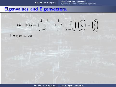
(A− λI) x =
2− λ −3 −10 −1− λ 0−1 1 2− λ
x1x2x3
=
000
The eigenvalues are the roots of the equation
|A− λI| =
∣∣∣∣∣∣2− λ −3 −1
0 −1− λ 0−1 1 2− λ
∣∣∣∣∣∣ = −
∣∣∣∣∣∣2− λ −3 −1−1 1 2− λ0 −1− λ 0
∣∣∣∣∣∣ =
∣∣∣∣∣∣−1 1 2− λ
2− λ −3 −10 −1− λ 0
∣∣∣∣∣∣ =
∣∣∣∣∣∣−1 1 2− λ0 −1− λ (2− λ)2 − 10 −1− λ 0
∣∣∣∣∣∣ =
Dr. Marco A Roque Sol Linear Algebra. Session 8

Abstract Linear AlgebraEigenvalues and Eigenvectors.Systems of Linear Differential Equations
Eigenvalues and Eigenvectors.
(A− λI) x =
2− λ −3 −10 −1− λ 0−1 1 2− λ
x1x2x3
=
000
The eigenvalues are the roots of the equation
|A− λI| =
∣∣∣∣∣∣2− λ −3 −1
0 −1− λ 0−1 1 2− λ
∣∣∣∣∣∣ = −
∣∣∣∣∣∣2− λ −3 −1−1 1 2− λ0 −1− λ 0
∣∣∣∣∣∣ =
∣∣∣∣∣∣−1 1 2− λ
2− λ −3 −10 −1− λ 0
∣∣∣∣∣∣ =
∣∣∣∣∣∣−1 1 2− λ0 −1− λ (2− λ)2 − 10 −1− λ 0
∣∣∣∣∣∣ =
Dr. Marco A Roque Sol Linear Algebra. Session 8
Abstract Linear AlgebraEigenvalues and Eigenvectors.Systems of Linear Differential Equations
Eigenvalues and Eigenvectors.
(A− λI) x =
2− λ −3 −10 −1− λ 0−1 1 2− λ
x1x2x3
=
000
The eigenvalues
are the roots of the equation
|A− λI| =
∣∣∣∣∣∣2− λ −3 −1
0 −1− λ 0−1 1 2− λ
∣∣∣∣∣∣ = −
∣∣∣∣∣∣2− λ −3 −1−1 1 2− λ0 −1− λ 0
∣∣∣∣∣∣ =
∣∣∣∣∣∣−1 1 2− λ
2− λ −3 −10 −1− λ 0
∣∣∣∣∣∣ =
∣∣∣∣∣∣−1 1 2− λ0 −1− λ (2− λ)2 − 10 −1− λ 0
∣∣∣∣∣∣ =
Dr. Marco A Roque Sol Linear Algebra. Session 8

Abstract Linear AlgebraEigenvalues and Eigenvectors.Systems of Linear Differential Equations
Eigenvalues and Eigenvectors.
(A− λI) x =
2− λ −3 −10 −1− λ 0−1 1 2− λ
x1x2x3
=
000
The eigenvalues are the roots
of the equation
|A− λI| =
∣∣∣∣∣∣2− λ −3 −1
0 −1− λ 0−1 1 2− λ
∣∣∣∣∣∣ = −
∣∣∣∣∣∣2− λ −3 −1−1 1 2− λ0 −1− λ 0
∣∣∣∣∣∣ =
∣∣∣∣∣∣−1 1 2− λ
2− λ −3 −10 −1− λ 0
∣∣∣∣∣∣ =
∣∣∣∣∣∣−1 1 2− λ0 −1− λ (2− λ)2 − 10 −1− λ 0
∣∣∣∣∣∣ =
Dr. Marco A Roque Sol Linear Algebra. Session 8

Abstract Linear AlgebraEigenvalues and Eigenvectors.Systems of Linear Differential Equations
Eigenvalues and Eigenvectors.
(A− λI) x =
2− λ −3 −10 −1− λ 0−1 1 2− λ
x1x2x3
=
000
The eigenvalues are the roots of the equation
|A− λI| =
∣∣∣∣∣∣2− λ −3 −1
0 −1− λ 0−1 1 2− λ
∣∣∣∣∣∣ = −
∣∣∣∣∣∣2− λ −3 −1−1 1 2− λ0 −1− λ 0
∣∣∣∣∣∣ =
∣∣∣∣∣∣−1 1 2− λ
2− λ −3 −10 −1− λ 0
∣∣∣∣∣∣ =
∣∣∣∣∣∣−1 1 2− λ0 −1− λ (2− λ)2 − 10 −1− λ 0
∣∣∣∣∣∣ =
Dr. Marco A Roque Sol Linear Algebra. Session 8

Abstract Linear AlgebraEigenvalues and Eigenvectors.Systems of Linear Differential Equations
Eigenvalues and Eigenvectors.
(A− λI) x =
2− λ −3 −10 −1− λ 0−1 1 2− λ
x1x2x3
=
000
The eigenvalues are the roots of the equation
|A− λI| =
∣∣∣∣∣∣2− λ −3 −1
0 −1− λ 0−1 1 2− λ
∣∣∣∣∣∣ =
−
∣∣∣∣∣∣2− λ −3 −1−1 1 2− λ0 −1− λ 0
∣∣∣∣∣∣ =
∣∣∣∣∣∣−1 1 2− λ
2− λ −3 −10 −1− λ 0
∣∣∣∣∣∣ =
∣∣∣∣∣∣−1 1 2− λ0 −1− λ (2− λ)2 − 10 −1− λ 0
∣∣∣∣∣∣ =
Dr. Marco A Roque Sol Linear Algebra. Session 8

Abstract Linear AlgebraEigenvalues and Eigenvectors.Systems of Linear Differential Equations
Eigenvalues and Eigenvectors.
(A− λI) x =
2− λ −3 −10 −1− λ 0−1 1 2− λ
x1x2x3
=
000
The eigenvalues are the roots of the equation
|A− λI| =
∣∣∣∣∣∣2− λ −3 −1
0 −1− λ 0−1 1 2− λ
∣∣∣∣∣∣ = −
∣∣∣∣∣∣2− λ −3 −1−1 1 2− λ0 −1− λ 0
∣∣∣∣∣∣ =
∣∣∣∣∣∣−1 1 2− λ
2− λ −3 −10 −1− λ 0
∣∣∣∣∣∣ =
∣∣∣∣∣∣−1 1 2− λ0 −1− λ (2− λ)2 − 10 −1− λ 0
∣∣∣∣∣∣ =
Dr. Marco A Roque Sol Linear Algebra. Session 8

Abstract Linear AlgebraEigenvalues and Eigenvectors.Systems of Linear Differential Equations
Eigenvalues and Eigenvectors.
(A− λI) x =
2− λ −3 −10 −1− λ 0−1 1 2− λ
x1x2x3
=
000
The eigenvalues are the roots of the equation
|A− λI| =
∣∣∣∣∣∣2− λ −3 −1
0 −1− λ 0−1 1 2− λ
∣∣∣∣∣∣ = −
∣∣∣∣∣∣2− λ −3 −1−1 1 2− λ0 −1− λ 0
∣∣∣∣∣∣ =
∣∣∣∣∣∣−1 1 2− λ
2− λ −3 −10 −1− λ 0
∣∣∣∣∣∣ =
∣∣∣∣∣∣−1 1 2− λ0 −1− λ (2− λ)2 − 10 −1− λ 0
∣∣∣∣∣∣ =
Dr. Marco A Roque Sol Linear Algebra. Session 8

Abstract Linear AlgebraEigenvalues and Eigenvectors.Systems of Linear Differential Equations
Eigenvalues and Eigenvectors.
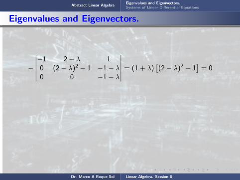
−
∣∣∣∣∣∣−1 2− λ 10 (2− λ)2 − 1 −1− λ0 0 −1− λ
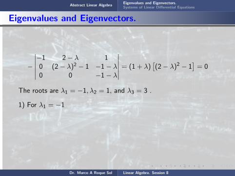
∣∣∣∣∣∣ = (1 + λ)[(2− λ)2 − 1
]= 0
The roots are λ1 = −1, λ2 = 1, and λ3 = 3 .
1) For λ1 = −1
(A− λ1I) x =
2− λ −3 −10 −1− λ 0−1 1 2− λ
=
Dr. Marco A Roque Sol Linear Algebra. Session 8

Abstract Linear AlgebraEigenvalues and Eigenvectors.Systems of Linear Differential Equations
Eigenvalues and Eigenvectors.
−
∣∣∣∣∣∣−1 2− λ 10 (2− λ)2 − 1 −1− λ0 0 −1− λ
∣∣∣∣∣∣ =
(1 + λ)[(2− λ)2 − 1
]= 0
The roots are λ1 = −1, λ2 = 1, and λ3 = 3 .
1) For λ1 = −1
(A− λ1I) x =
2− λ −3 −10 −1− λ 0−1 1 2− λ
=
Dr. Marco A Roque Sol Linear Algebra. Session 8
Abstract Linear AlgebraEigenvalues and Eigenvectors.Systems of Linear Differential Equations
Eigenvalues and Eigenvectors.
−
∣∣∣∣∣∣−1 2− λ 10 (2− λ)2 − 1 −1− λ0 0 −1− λ
∣∣∣∣∣∣ = (1 + λ)[(2− λ)2 − 1
]= 0
The roots are λ1 = −1, λ2 = 1, and λ3 = 3 .
1) For λ1 = −1
(A− λ1I) x =
2− λ −3 −10 −1− λ 0−1 1 2− λ
=
Dr. Marco A Roque Sol Linear Algebra. Session 8

Abstract Linear AlgebraEigenvalues and Eigenvectors.Systems of Linear Differential Equations
Eigenvalues and Eigenvectors.
−
∣∣∣∣∣∣−1 2− λ 10 (2− λ)2 − 1 −1− λ0 0 −1− λ
∣∣∣∣∣∣ = (1 + λ)[(2− λ)2 − 1
]= 0
The roots are
λ1 = −1, λ2 = 1, and λ3 = 3 .
1) For λ1 = −1
(A− λ1I) x =
2− λ −3 −10 −1− λ 0−1 1 2− λ
=
Dr. Marco A Roque Sol Linear Algebra. Session 8

Abstract Linear AlgebraEigenvalues and Eigenvectors.Systems of Linear Differential Equations
Eigenvalues and Eigenvectors.
−
∣∣∣∣∣∣−1 2− λ 10 (2− λ)2 − 1 −1− λ0 0 −1− λ
∣∣∣∣∣∣ = (1 + λ)[(2− λ)2 − 1
]= 0
The roots are λ1 = −1, λ2 = 1, and λ3 = 3 .
1) For λ1 = −1
(A− λ1I) x =
2− λ −3 −10 −1− λ 0−1 1 2− λ
=
Dr. Marco A Roque Sol Linear Algebra. Session 8

Abstract Linear AlgebraEigenvalues and Eigenvectors.Systems of Linear Differential Equations
Eigenvalues and Eigenvectors.
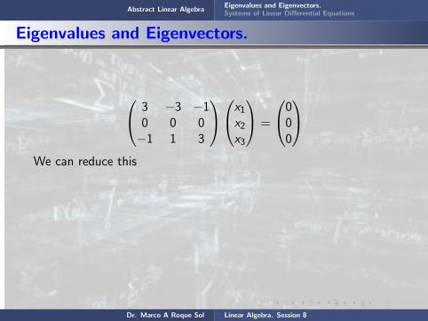
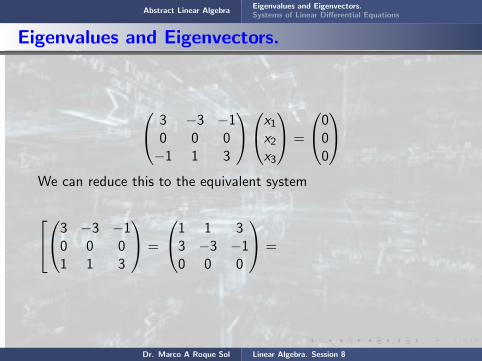
3 −3 −10 0 0−1 1 3
x1x2x3
=
000
We can reduce this to the equivalent system
3 −3 −10 0 01 1 3
=
1 1 33 −3 −10 0 0
=
1 1 30 0 80 0 0
x1x2x3
=
000
Dr. Marco A Roque Sol Linear Algebra. Session 8

Abstract Linear AlgebraEigenvalues and Eigenvectors.Systems of Linear Differential Equations
Eigenvalues and Eigenvectors.
3 −3 −10 0 0−1 1 3
x1x2x3
=
000
We can
reduce this to the equivalent system
3 −3 −10 0 01 1 3
=
1 1 33 −3 −10 0 0
=
1 1 30 0 80 0 0
x1x2x3
=
000
Dr. Marco A Roque Sol Linear Algebra. Session 8
Abstract Linear AlgebraEigenvalues and Eigenvectors.Systems of Linear Differential Equations
Eigenvalues and Eigenvectors.
3 −3 −10 0 0−1 1 3
x1x2x3
=
000
We can reduce this
to the equivalent system
3 −3 −10 0 01 1 3
=
1 1 33 −3 −10 0 0
=
1 1 30 0 80 0 0
x1x2x3
=
000
Dr. Marco A Roque Sol Linear Algebra. Session 8

Abstract Linear AlgebraEigenvalues and Eigenvectors.Systems of Linear Differential Equations
Eigenvalues and Eigenvectors.
3 −3 −10 0 0−1 1 3
x1x2x3
=
000
We can reduce this to the equivalent system
3 −3 −10 0 01 1 3
=
1 1 33 −3 −10 0 0
=
1 1 30 0 80 0 0
x1x2x3
=
000
Dr. Marco A Roque Sol Linear Algebra. Session 8

Abstract Linear AlgebraEigenvalues and Eigenvectors.Systems of Linear Differential Equations
Eigenvalues and Eigenvectors.
3 −3 −10 0 0−1 1 3
x1x2x3
=
000
We can reduce this to the equivalent system
3 −3 −10 0 01 1 3
=
1 1 33 −3 −10 0 0
=
1 1 30 0 80 0 0
x1x2x3
=
000
Dr. Marco A Roque Sol Linear Algebra. Session 8
Abstract Linear AlgebraEigenvalues and Eigenvectors.Systems of Linear Differential Equations
Eigenvalues and Eigenvectors.
The above system is reduced immediately to the equations
x1 + x2 + 3x3 = 0 8x3 = 0
One equation and two unknowns. Hence, one of them is freevariable, let’s say x2 = α. Therefore we have x1 = −x2 = −α, andx3 = 0 . Thus, we get
x =
−αα0
= α
1−10
; α = real number
Dr. Marco A Roque Sol Linear Algebra. Session 8

Abstract Linear AlgebraEigenvalues and Eigenvectors.Systems of Linear Differential Equations
Eigenvalues and Eigenvectors.
The above system
is reduced immediately to the equations
x1 + x2 + 3x3 = 0 8x3 = 0
One equation and two unknowns. Hence, one of them is freevariable, let’s say x2 = α. Therefore we have x1 = −x2 = −α, andx3 = 0 . Thus, we get
x =
−αα0
= α
1−10
; α = real number
Dr. Marco A Roque Sol Linear Algebra. Session 8
Abstract Linear AlgebraEigenvalues and Eigenvectors.Systems of Linear Differential Equations
Eigenvalues and Eigenvectors.
The above system is reduced immediately to
the equations
x1 + x2 + 3x3 = 0 8x3 = 0
One equation and two unknowns. Hence, one of them is freevariable, let’s say x2 = α. Therefore we have x1 = −x2 = −α, andx3 = 0 . Thus, we get
x =
−αα0
= α
1−10
; α = real number
Dr. Marco A Roque Sol Linear Algebra. Session 8

Abstract Linear AlgebraEigenvalues and Eigenvectors.Systems of Linear Differential Equations
Eigenvalues and Eigenvectors.
The above system is reduced immediately to the equations
x1 + x2 + 3x3 = 0 8x3 = 0
One equation and two unknowns. Hence, one of them is freevariable, let’s say x2 = α. Therefore we have x1 = −x2 = −α, andx3 = 0 . Thus, we get
x =
−αα0
= α
1−10
; α = real number
Dr. Marco A Roque Sol Linear Algebra. Session 8

Abstract Linear AlgebraEigenvalues and Eigenvectors.Systems of Linear Differential Equations
Eigenvalues and Eigenvectors.
The above system is reduced immediately to the equations
x1 + x2 + 3x3 = 0 8x3 = 0
One equation and two unknowns. Hence,
one of them is freevariable, let’s say x2 = α. Therefore we have x1 = −x2 = −α, andx3 = 0 . Thus, we get
x =
−αα0
= α
1−10
; α = real number
Dr. Marco A Roque Sol Linear Algebra. Session 8

Abstract Linear AlgebraEigenvalues and Eigenvectors.Systems of Linear Differential Equations
Eigenvalues and Eigenvectors.
The above system is reduced immediately to the equations
x1 + x2 + 3x3 = 0 8x3 = 0
One equation and two unknowns. Hence, one of them is freevariable,
let’s say x2 = α. Therefore we have x1 = −x2 = −α, andx3 = 0 . Thus, we get
x =
−αα0
= α
1−10
; α = real number
Dr. Marco A Roque Sol Linear Algebra. Session 8
Abstract Linear AlgebraEigenvalues and Eigenvectors.Systems of Linear Differential Equations
Eigenvalues and Eigenvectors.
The above system is reduced immediately to the equations
x1 + x2 + 3x3 = 0 8x3 = 0
One equation and two unknowns. Hence, one of them is freevariable, let’s say x2 = α.
Therefore we have x1 = −x2 = −α, andx3 = 0 . Thus, we get
x =
−αα0
= α
1−10
; α = real number
Dr. Marco A Roque Sol Linear Algebra. Session 8

Abstract Linear AlgebraEigenvalues and Eigenvectors.Systems of Linear Differential Equations
Eigenvalues and Eigenvectors.
The above system is reduced immediately to the equations
x1 + x2 + 3x3 = 0 8x3 = 0
One equation and two unknowns. Hence, one of them is freevariable, let’s say x2 = α. Therefore we have
x1 = −x2 = −α, andx3 = 0 . Thus, we get
x =
−αα0
= α
1−10
; α = real number
Dr. Marco A Roque Sol Linear Algebra. Session 8

Abstract Linear AlgebraEigenvalues and Eigenvectors.Systems of Linear Differential Equations
Eigenvalues and Eigenvectors.
The above system is reduced immediately to the equations
x1 + x2 + 3x3 = 0 8x3 = 0
One equation and two unknowns. Hence, one of them is freevariable, let’s say x2 = α. Therefore we have x1 = −x2 = −α, and
x3 = 0 . Thus, we get
x =
−αα0
= α
1−10
; α = real number
Dr. Marco A Roque Sol Linear Algebra. Session 8

Abstract Linear AlgebraEigenvalues and Eigenvectors.Systems of Linear Differential Equations
Eigenvalues and Eigenvectors.
The above system is reduced immediately to the equations
x1 + x2 + 3x3 = 0 8x3 = 0
One equation and two unknowns. Hence, one of them is freevariable, let’s say x2 = α. Therefore we have x1 = −x2 = −α, andx3 = 0 .
Thus, we get
x =
−αα0
= α
1−10
; α = real number
Dr. Marco A Roque Sol Linear Algebra. Session 8

Abstract Linear AlgebraEigenvalues and Eigenvectors.Systems of Linear Differential Equations
Eigenvalues and Eigenvectors.
The above system is reduced immediately to the equations
x1 + x2 + 3x3 = 0 8x3 = 0
One equation and two unknowns. Hence, one of them is freevariable, let’s say x2 = α. Therefore we have x1 = −x2 = −α, andx3 = 0 . Thus, we get
x =
−αα0
= α
1−10
; α = real number
Dr. Marco A Roque Sol Linear Algebra. Session 8

Abstract Linear AlgebraEigenvalues and Eigenvectors.Systems of Linear Differential Equations
Eigenvalues and Eigenvectors.
The above system is reduced immediately to the equations
x1 + x2 + 3x3 = 0 8x3 = 0
One equation and two unknowns. Hence, one of them is freevariable, let’s say x2 = α. Therefore we have x1 = −x2 = −α, andx3 = 0 . Thus, we get
x =
−αα0
= α
1−10
; α = real number
Dr. Marco A Roque Sol Linear Algebra. Session 8

Abstract Linear AlgebraEigenvalues and Eigenvectors.Systems of Linear Differential Equations
Eigenvalues and Eigenvectors.
A particular eigenvector is
x(1) =
1−10
2) For λ2 = 1
(A− λ2I) x =
2− λ −3 −10 −1− λ 0−1 1 2− λ
x1x2x3
=
1 −3 −10 −2 0−1 1 1
x1x2x3
=
Dr. Marco A Roque Sol Linear Algebra. Session 8
Abstract Linear AlgebraEigenvalues and Eigenvectors.Systems of Linear Differential Equations
Eigenvalues and Eigenvectors.
A particular
eigenvector is
x(1) =
1−10
2) For λ2 = 1
(A− λ2I) x =
2− λ −3 −10 −1− λ 0−1 1 2− λ
x1x2x3
=
1 −3 −10 −2 0−1 1 1
x1x2x3
=
Dr. Marco A Roque Sol Linear Algebra. Session 8

Abstract Linear AlgebraEigenvalues and Eigenvectors.Systems of Linear Differential Equations
Eigenvalues and Eigenvectors.
A particular eigenvector is
x(1) =
1−10
2) For λ2 = 1
(A− λ2I) x =
2− λ −3 −10 −1− λ 0−1 1 2− λ
x1x2x3
=
1 −3 −10 −2 0−1 1 1
x1x2x3
=
Dr. Marco A Roque Sol Linear Algebra. Session 8
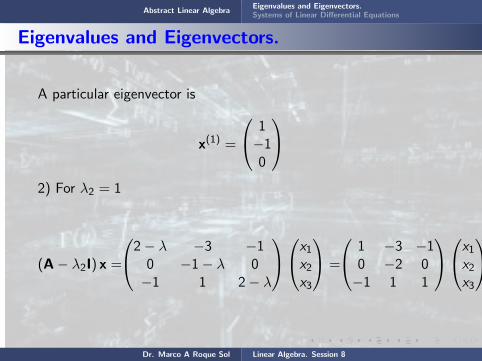

Abstract Linear AlgebraEigenvalues and Eigenvectors.Systems of Linear Differential Equations
Eigenvalues and Eigenvectors.
1 −3 −10 −2 00 −2 0
=
1 −3 −10 −2 00 0 0
x1x2x3
=
000
The above system is reduced immediately to the equations
x1 − 3x2 − x3 = 0 − 2x2 = 0
One equation and two unknowns. Hence, one of them is freevariable, let’s say x3 = α. Therefore we have x1 = x3 = α, andx2 = 0 . Thus, we get
Dr. Marco A Roque Sol Linear Algebra. Session 8
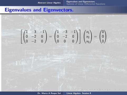
Abstract Linear AlgebraEigenvalues and Eigenvectors.Systems of Linear Differential Equations
Eigenvalues and Eigenvectors.
1 −3 −10 −2 00 −2 0
=
1 −3 −10 −2 00 0 0
x1x2x3
=
000
The above system is reduced immediately to the equations
x1 − 3x2 − x3 = 0 − 2x2 = 0
One equation and two unknowns. Hence, one of them is freevariable, let’s say x3 = α. Therefore we have x1 = x3 = α, andx2 = 0 . Thus, we get
Dr. Marco A Roque Sol Linear Algebra. Session 8
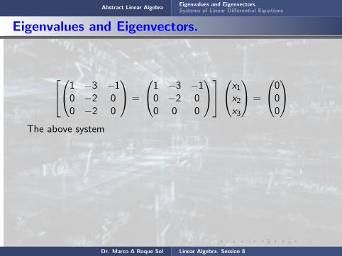
Abstract Linear AlgebraEigenvalues and Eigenvectors.Systems of Linear Differential Equations
Eigenvalues and Eigenvectors.
1 −3 −10 −2 00 −2 0
=
1 −3 −10 −2 00 0 0
x1x2x3
=
000
The above system
is reduced immediately to the equations
x1 − 3x2 − x3 = 0 − 2x2 = 0
One equation and two unknowns. Hence, one of them is freevariable, let’s say x3 = α. Therefore we have x1 = x3 = α, andx2 = 0 . Thus, we get
Dr. Marco A Roque Sol Linear Algebra. Session 8
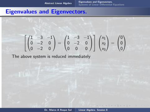
Abstract Linear AlgebraEigenvalues and Eigenvectors.Systems of Linear Differential Equations
Eigenvalues and Eigenvectors.
1 −3 −10 −2 00 −2 0
=
1 −3 −10 −2 00 0 0
x1x2x3
=
000
The above system is reduced immediately
to the equations
x1 − 3x2 − x3 = 0 − 2x2 = 0
One equation and two unknowns. Hence, one of them is freevariable, let’s say x3 = α. Therefore we have x1 = x3 = α, andx2 = 0 . Thus, we get
Dr. Marco A Roque Sol Linear Algebra. Session 8

Abstract Linear AlgebraEigenvalues and Eigenvectors.Systems of Linear Differential Equations
Eigenvalues and Eigenvectors.
1 −3 −10 −2 00 −2 0
=
1 −3 −10 −2 00 0 0
x1x2x3
=
000
The above system is reduced immediately to the equations
x1 − 3x2 − x3 = 0 − 2x2 = 0
One equation and two unknowns. Hence, one of them is freevariable, let’s say x3 = α. Therefore we have x1 = x3 = α, andx2 = 0 . Thus, we get
Dr. Marco A Roque Sol Linear Algebra. Session 8
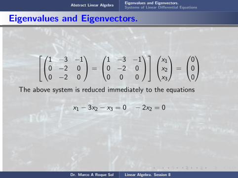
Abstract Linear AlgebraEigenvalues and Eigenvectors.Systems of Linear Differential Equations
Eigenvalues and Eigenvectors.
1 −3 −10 −2 00 −2 0
=
1 −3 −10 −2 00 0 0
x1x2x3
=
000
The above system is reduced immediately to the equations
x1 − 3x2 − x3 = 0 − 2x2 = 0
One equation and
two unknowns. Hence, one of them is freevariable, let’s say x3 = α. Therefore we have x1 = x3 = α, andx2 = 0 . Thus, we get
Dr. Marco A Roque Sol Linear Algebra. Session 8

Abstract Linear AlgebraEigenvalues and Eigenvectors.Systems of Linear Differential Equations
Eigenvalues and Eigenvectors.
1 −3 −10 −2 00 −2 0
=
1 −3 −10 −2 00 0 0
x1x2x3
=
000
The above system is reduced immediately to the equations
x1 − 3x2 − x3 = 0 − 2x2 = 0
One equation and two unknowns.
Hence, one of them is freevariable, let’s say x3 = α. Therefore we have x1 = x3 = α, andx2 = 0 . Thus, we get
Dr. Marco A Roque Sol Linear Algebra. Session 8

Abstract Linear AlgebraEigenvalues and Eigenvectors.Systems of Linear Differential Equations
Eigenvalues and Eigenvectors.
1 −3 −10 −2 00 −2 0
=
1 −3 −10 −2 00 0 0
x1x2x3
=
000
The above system is reduced immediately to the equations
x1 − 3x2 − x3 = 0 − 2x2 = 0
One equation and two unknowns. Hence,
one of them is freevariable, let’s say x3 = α. Therefore we have x1 = x3 = α, andx2 = 0 . Thus, we get
Dr. Marco A Roque Sol Linear Algebra. Session 8
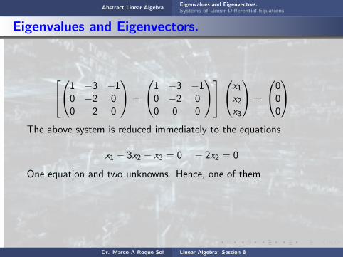
Abstract Linear AlgebraEigenvalues and Eigenvectors.Systems of Linear Differential Equations
Eigenvalues and Eigenvectors.
1 −3 −10 −2 00 −2 0
=
1 −3 −10 −2 00 0 0
x1x2x3
=
000
The above system is reduced immediately to the equations
x1 − 3x2 − x3 = 0 − 2x2 = 0
One equation and two unknowns. Hence, one of them
is freevariable, let’s say x3 = α. Therefore we have x1 = x3 = α, andx2 = 0 . Thus, we get
Dr. Marco A Roque Sol Linear Algebra. Session 8

Abstract Linear AlgebraEigenvalues and Eigenvectors.Systems of Linear Differential Equations
Eigenvalues and Eigenvectors.
1 −3 −10 −2 00 −2 0
=
1 −3 −10 −2 00 0 0
x1x2x3
=
000
The above system is reduced immediately to the equations
x1 − 3x2 − x3 = 0 − 2x2 = 0
One equation and two unknowns. Hence, one of them is freevariable,
let’s say x3 = α. Therefore we have x1 = x3 = α, andx2 = 0 . Thus, we get
Dr. Marco A Roque Sol Linear Algebra. Session 8
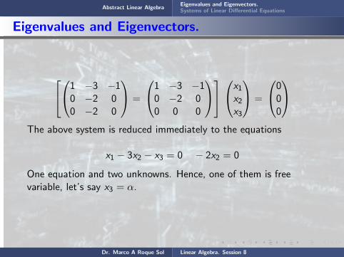
Abstract Linear AlgebraEigenvalues and Eigenvectors.Systems of Linear Differential Equations
Eigenvalues and Eigenvectors.
1 −3 −10 −2 00 −2 0
=
1 −3 −10 −2 00 0 0
x1x2x3
=
000
The above system is reduced immediately to the equations
x1 − 3x2 − x3 = 0 − 2x2 = 0
One equation and two unknowns. Hence, one of them is freevariable, let’s say x3 = α.
Therefore we have x1 = x3 = α, andx2 = 0 . Thus, we get
Dr. Marco A Roque Sol Linear Algebra. Session 8
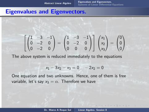
Abstract Linear AlgebraEigenvalues and Eigenvectors.Systems of Linear Differential Equations
Eigenvalues and Eigenvectors.
1 −3 −10 −2 00 −2 0
=
1 −3 −10 −2 00 0 0
x1x2x3
=
000
The above system is reduced immediately to the equations
x1 − 3x2 − x3 = 0 − 2x2 = 0
One equation and two unknowns. Hence, one of them is freevariable, let’s say x3 = α. Therefore we have
x1 = x3 = α, andx2 = 0 . Thus, we get
Dr. Marco A Roque Sol Linear Algebra. Session 8
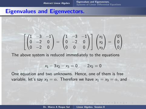
Abstract Linear AlgebraEigenvalues and Eigenvectors.Systems of Linear Differential Equations
Eigenvalues and Eigenvectors.
1 −3 −10 −2 00 −2 0
=
1 −3 −10 −2 00 0 0
x1x2x3
=
000
The above system is reduced immediately to the equations
x1 − 3x2 − x3 = 0 − 2x2 = 0
One equation and two unknowns. Hence, one of them is freevariable, let’s say x3 = α. Therefore we have x1 = x3 = α, and
x2 = 0 . Thus, we get
Dr. Marco A Roque Sol Linear Algebra. Session 8

Abstract Linear AlgebraEigenvalues and Eigenvectors.Systems of Linear Differential Equations
Eigenvalues and Eigenvectors.
1 −3 −10 −2 00 −2 0
=
1 −3 −10 −2 00 0 0
x1x2x3
=
000
The above system is reduced immediately to the equations
x1 − 3x2 − x3 = 0 − 2x2 = 0
One equation and two unknowns. Hence, one of them is freevariable, let’s say x3 = α. Therefore we have x1 = x3 = α, andx2 = 0 .
Thus, we get
Dr. Marco A Roque Sol Linear Algebra. Session 8

Abstract Linear AlgebraEigenvalues and Eigenvectors.Systems of Linear Differential Equations
Eigenvalues and Eigenvectors.
1 −3 −10 −2 00 −2 0
=
1 −3 −10 −2 00 0 0
x1x2x3
=
000
The above system is reduced immediately to the equations
x1 − 3x2 − x3 = 0 − 2x2 = 0
One equation and two unknowns. Hence, one of them is freevariable, let’s say x3 = α. Therefore we have x1 = x3 = α, andx2 = 0 . Thus, we get
Dr. Marco A Roque Sol Linear Algebra. Session 8

Abstract Linear AlgebraEigenvalues and Eigenvectors.Systems of Linear Differential Equations
Eigenvalues ansd Eigenvectors.
x =
α0α
= α
101
; α = real number
A particular eigenvector is given by
x(1) =
101
3) For λ3 = 3
(A− λ3I) x =
2− λ −3 −10 −1− λ 0−1 1 2− λ
=
Dr. Marco A Roque Sol Linear Algebra. Session 8
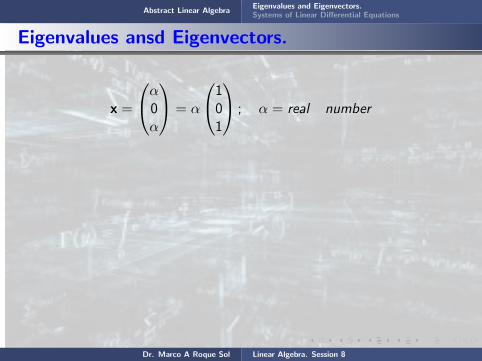
Abstract Linear AlgebraEigenvalues and Eigenvectors.Systems of Linear Differential Equations
Eigenvalues ansd Eigenvectors.
x =
α0α
= α
101
; α = real number
A particular eigenvector is given by
x(1) =
101
3) For λ3 = 3
(A− λ3I) x =
2− λ −3 −10 −1− λ 0−1 1 2− λ
=
Dr. Marco A Roque Sol Linear Algebra. Session 8

Abstract Linear AlgebraEigenvalues and Eigenvectors.Systems of Linear Differential Equations
Eigenvalues ansd Eigenvectors.
x =
α0α
= α
101
; α = real number
A particular
eigenvector is given by
x(1) =
101
3) For λ3 = 3
(A− λ3I) x =
2− λ −3 −10 −1− λ 0−1 1 2− λ
=
Dr. Marco A Roque Sol Linear Algebra. Session 8

Abstract Linear AlgebraEigenvalues and Eigenvectors.Systems of Linear Differential Equations
Eigenvalues ansd Eigenvectors.
x =
α0α
= α
101
; α = real number
A particular eigenvector
is given by
x(1) =
101
3) For λ3 = 3
(A− λ3I) x =
2− λ −3 −10 −1− λ 0−1 1 2− λ
=
Dr. Marco A Roque Sol Linear Algebra. Session 8

Abstract Linear AlgebraEigenvalues and Eigenvectors.Systems of Linear Differential Equations
Eigenvalues ansd Eigenvectors.
x =
α0α
= α
101
; α = real number
A particular eigenvector is given by
x(1) =
101
3) For λ3 = 3
(A− λ3I) x =
2− λ −3 −10 −1− λ 0−1 1 2− λ
=
Dr. Marco A Roque Sol Linear Algebra. Session 8
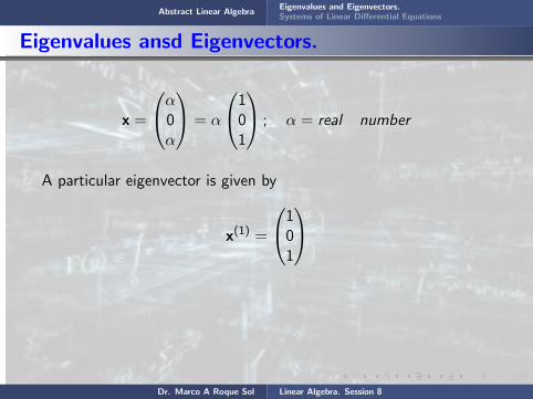
Abstract Linear AlgebraEigenvalues and Eigenvectors.Systems of Linear Differential Equations
Eigenvalues ansd Eigenvectors.
x =
α0α
= α
101
; α = real number
A particular eigenvector is given by
x(1) =
101
3) For λ3 = 3
(A− λ3I) x =
2− λ −3 −10 −1− λ 0−1 1 2− λ
=
Dr. Marco A Roque Sol Linear Algebra. Session 8

Abstract Linear AlgebraEigenvalues and Eigenvectors.Systems of Linear Differential Equations
Eigenvalues ansd Eigenvectors.
−1 −3 −10 −4 0−1 1 −1
=
−1 −3 −10 −4 00 4 0
=
−1 −3 −10 −4 00 0 0
x1x2x3
=
000
The above system is reduced immediately to the equations
−x1 − 3x2 − x3 = 0 − 4x2 = 0
One equation and two unknowns. Hence, one of them is a freevariable, let’s say x3 = α. Therefore we have x1 = −x3 = −α, andx2 = 0 . Thus, we get
Dr. Marco A Roque Sol Linear Algebra. Session 8
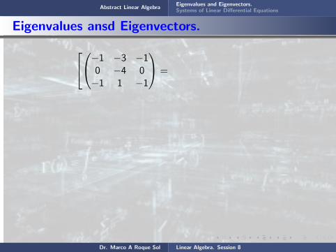
Abstract Linear AlgebraEigenvalues and Eigenvectors.Systems of Linear Differential Equations
Eigenvalues ansd Eigenvectors.
−1 −3 −10 −4 0−1 1 −1
=
−1 −3 −10 −4 00 4 0
=
−1 −3 −10 −4 00 0 0
x1x2x3
=
000
The above system is reduced immediately to the equations
−x1 − 3x2 − x3 = 0 − 4x2 = 0
One equation and two unknowns. Hence, one of them is a freevariable, let’s say x3 = α. Therefore we have x1 = −x3 = −α, andx2 = 0 . Thus, we get
Dr. Marco A Roque Sol Linear Algebra. Session 8
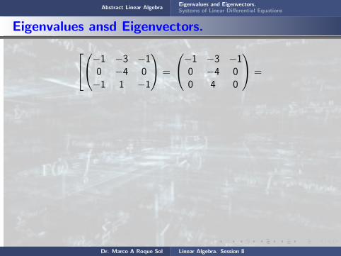
Abstract Linear AlgebraEigenvalues and Eigenvectors.Systems of Linear Differential Equations
Eigenvalues ansd Eigenvectors.
−1 −3 −10 −4 0−1 1 −1
=
−1 −3 −10 −4 00 4 0
=
−1 −3 −10 −4 00 0 0
x1x2x3
=
000
The above system is reduced immediately to the equations
−x1 − 3x2 − x3 = 0 − 4x2 = 0
One equation and two unknowns. Hence, one of them is a freevariable, let’s say x3 = α. Therefore we have x1 = −x3 = −α, andx2 = 0 . Thus, we get
Dr. Marco A Roque Sol Linear Algebra. Session 8

Abstract Linear AlgebraEigenvalues and Eigenvectors.Systems of Linear Differential Equations
Eigenvalues ansd Eigenvectors.
−1 −3 −10 −4 0−1 1 −1
=
−1 −3 −10 −4 00 4 0
=
−1 −3 −10 −4 00 0 0
x1x2x3
=
000
The above system
is reduced immediately to the equations
−x1 − 3x2 − x3 = 0 − 4x2 = 0
One equation and two unknowns. Hence, one of them is a freevariable, let’s say x3 = α. Therefore we have x1 = −x3 = −α, andx2 = 0 . Thus, we get
Dr. Marco A Roque Sol Linear Algebra. Session 8

Abstract Linear AlgebraEigenvalues and Eigenvectors.Systems of Linear Differential Equations
Eigenvalues ansd Eigenvectors.
−1 −3 −10 −4 0−1 1 −1
=
−1 −3 −10 −4 00 4 0
=
−1 −3 −10 −4 00 0 0
x1x2x3
=
000
The above system is reduced immediately
to the equations
−x1 − 3x2 − x3 = 0 − 4x2 = 0
One equation and two unknowns. Hence, one of them is a freevariable, let’s say x3 = α. Therefore we have x1 = −x3 = −α, andx2 = 0 . Thus, we get
Dr. Marco A Roque Sol Linear Algebra. Session 8

Abstract Linear AlgebraEigenvalues and Eigenvectors.Systems of Linear Differential Equations
Eigenvalues ansd Eigenvectors.
−1 −3 −10 −4 0−1 1 −1
=
−1 −3 −10 −4 00 4 0
=
−1 −3 −10 −4 00 0 0
x1x2x3
=
000
The above system is reduced immediately to the equations
−x1 − 3x2 − x3 = 0 − 4x2 = 0
One equation and two unknowns. Hence, one of them is a freevariable, let’s say x3 = α. Therefore we have x1 = −x3 = −α, andx2 = 0 . Thus, we get
Dr. Marco A Roque Sol Linear Algebra. Session 8

Abstract Linear AlgebraEigenvalues and Eigenvectors.Systems of Linear Differential Equations
Eigenvalues ansd Eigenvectors.
−1 −3 −10 −4 0−1 1 −1
=
−1 −3 −10 −4 00 4 0
=
−1 −3 −10 −4 00 0 0
x1x2x3
=
000
The above system is reduced immediately to the equations
−x1 − 3x2 − x3 = 0 − 4x2 = 0
One equation and
two unknowns. Hence, one of them is a freevariable, let’s say x3 = α. Therefore we have x1 = −x3 = −α, andx2 = 0 . Thus, we get
Dr. Marco A Roque Sol Linear Algebra. Session 8

Abstract Linear AlgebraEigenvalues and Eigenvectors.Systems of Linear Differential Equations
Eigenvalues ansd Eigenvectors.
−1 −3 −10 −4 0−1 1 −1
=
−1 −3 −10 −4 00 4 0
=
−1 −3 −10 −4 00 0 0
x1x2x3
=
000
The above system is reduced immediately to the equations
−x1 − 3x2 − x3 = 0 − 4x2 = 0
One equation and two unknowns.
Hence, one of them is a freevariable, let’s say x3 = α. Therefore we have x1 = −x3 = −α, andx2 = 0 . Thus, we get
Dr. Marco A Roque Sol Linear Algebra. Session 8

Abstract Linear AlgebraEigenvalues and Eigenvectors.Systems of Linear Differential Equations
Eigenvalues ansd Eigenvectors.
−1 −3 −10 −4 0−1 1 −1
=
−1 −3 −10 −4 00 4 0
=
−1 −3 −10 −4 00 0 0
x1x2x3
=
000
The above system is reduced immediately to the equations
−x1 − 3x2 − x3 = 0 − 4x2 = 0
One equation and two unknowns. Hence,
one of them is a freevariable, let’s say x3 = α. Therefore we have x1 = −x3 = −α, andx2 = 0 . Thus, we get
Dr. Marco A Roque Sol Linear Algebra. Session 8

Abstract Linear AlgebraEigenvalues and Eigenvectors.Systems of Linear Differential Equations
Eigenvalues ansd Eigenvectors.
−1 −3 −10 −4 0−1 1 −1
=
−1 −3 −10 −4 00 4 0
=
−1 −3 −10 −4 00 0 0
x1x2x3
=
000
The above system is reduced immediately to the equations
−x1 − 3x2 − x3 = 0 − 4x2 = 0
One equation and two unknowns. Hence, one of them
is a freevariable, let’s say x3 = α. Therefore we have x1 = −x3 = −α, andx2 = 0 . Thus, we get
Dr. Marco A Roque Sol Linear Algebra. Session 8

Abstract Linear AlgebraEigenvalues and Eigenvectors.Systems of Linear Differential Equations
Eigenvalues ansd Eigenvectors.
−1 −3 −10 −4 0−1 1 −1
=
−1 −3 −10 −4 00 4 0
=
−1 −3 −10 −4 00 0 0
x1x2x3
=
000
The above system is reduced immediately to the equations
−x1 − 3x2 − x3 = 0 − 4x2 = 0
One equation and two unknowns. Hence, one of them is a freevariable,
let’s say x3 = α. Therefore we have x1 = −x3 = −α, andx2 = 0 . Thus, we get
Dr. Marco A Roque Sol Linear Algebra. Session 8
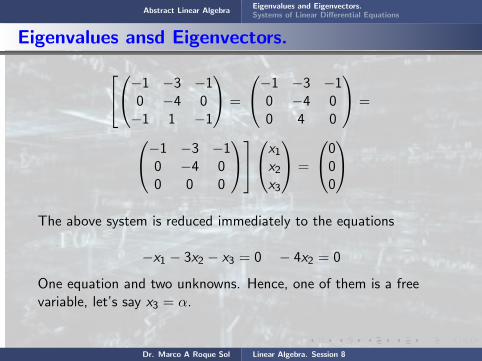
Abstract Linear AlgebraEigenvalues and Eigenvectors.Systems of Linear Differential Equations
Eigenvalues ansd Eigenvectors.
−1 −3 −10 −4 0−1 1 −1
=
−1 −3 −10 −4 00 4 0
=
−1 −3 −10 −4 00 0 0
x1x2x3
=
000
The above system is reduced immediately to the equations
−x1 − 3x2 − x3 = 0 − 4x2 = 0
One equation and two unknowns. Hence, one of them is a freevariable, let’s say x3 = α.
Therefore we have x1 = −x3 = −α, andx2 = 0 . Thus, we get
Dr. Marco A Roque Sol Linear Algebra. Session 8
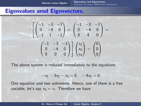
Abstract Linear AlgebraEigenvalues and Eigenvectors.Systems of Linear Differential Equations
Eigenvalues ansd Eigenvectors.
−1 −3 −10 −4 0−1 1 −1
=
−1 −3 −10 −4 00 4 0
=
−1 −3 −10 −4 00 0 0
x1x2x3
=
000
The above system is reduced immediately to the equations
−x1 − 3x2 − x3 = 0 − 4x2 = 0
One equation and two unknowns. Hence, one of them is a freevariable, let’s say x3 = α. Therefore we have
x1 = −x3 = −α, andx2 = 0 . Thus, we get
Dr. Marco A Roque Sol Linear Algebra. Session 8
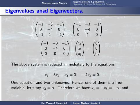
Abstract Linear AlgebraEigenvalues and Eigenvectors.Systems of Linear Differential Equations
Eigenvalues ansd Eigenvectors.
−1 −3 −10 −4 0−1 1 −1
=
−1 −3 −10 −4 00 4 0
=
−1 −3 −10 −4 00 0 0
x1x2x3
=
000
The above system is reduced immediately to the equations
−x1 − 3x2 − x3 = 0 − 4x2 = 0
One equation and two unknowns. Hence, one of them is a freevariable, let’s say x3 = α. Therefore we have x1 = −x3 = −α, and
x2 = 0 . Thus, we get
Dr. Marco A Roque Sol Linear Algebra. Session 8

Abstract Linear AlgebraEigenvalues and Eigenvectors.Systems of Linear Differential Equations
Eigenvalues ansd Eigenvectors.
−1 −3 −10 −4 0−1 1 −1
=
−1 −3 −10 −4 00 4 0
=
−1 −3 −10 −4 00 0 0
x1x2x3
=
000
The above system is reduced immediately to the equations
−x1 − 3x2 − x3 = 0 − 4x2 = 0
One equation and two unknowns. Hence, one of them is a freevariable, let’s say x3 = α. Therefore we have x1 = −x3 = −α, andx2 = 0 .
Thus, we get
Dr. Marco A Roque Sol Linear Algebra. Session 8

Abstract Linear AlgebraEigenvalues and Eigenvectors.Systems of Linear Differential Equations
Eigenvalues ansd Eigenvectors.
−1 −3 −10 −4 0−1 1 −1
=
−1 −3 −10 −4 00 4 0
=
−1 −3 −10 −4 00 0 0
x1x2x3
=
000
The above system is reduced immediately to the equations
−x1 − 3x2 − x3 = 0 − 4x2 = 0
One equation and two unknowns. Hence, one of them is a freevariable, let’s say x3 = α. Therefore we have x1 = −x3 = −α, andx2 = 0 . Thus, we get
Dr. Marco A Roque Sol Linear Algebra. Session 8

Abstract Linear AlgebraEigenvalues and Eigenvectors.Systems of Linear Differential Equations
Eigenvalues ansd Eigenvectors.
x =
−α0α
= α
−101
; α = real number
A particular eigenvector is given by
x(1) =
−101
Dr. Marco A Roque Sol Linear Algebra. Session 8

Abstract Linear AlgebraEigenvalues and Eigenvectors.Systems of Linear Differential Equations
Eigenvalues ansd Eigenvectors.
x =
−α0α
= α
−101
; α = real number
A particular eigenvector is given by
x(1) =
−101
Dr. Marco A Roque Sol Linear Algebra. Session 8

Abstract Linear AlgebraEigenvalues and Eigenvectors.Systems of Linear Differential Equations
Eigenvalues ansd Eigenvectors.
x =
−α0α
=
α
−101
; α = real number
A particular eigenvector is given by
x(1) =
−101
Dr. Marco A Roque Sol Linear Algebra. Session 8
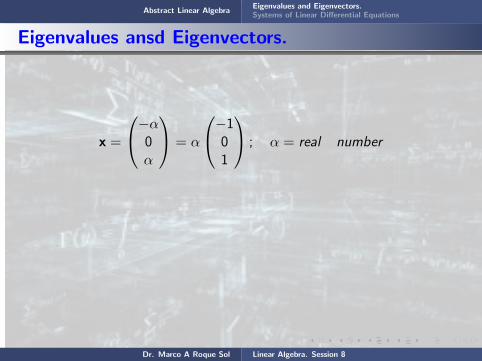
Abstract Linear AlgebraEigenvalues and Eigenvectors.Systems of Linear Differential Equations
Eigenvalues ansd Eigenvectors.
x =
−α0α
= α
−101
; α = real number
A particular eigenvector is given by
x(1) =
−101
Dr. Marco A Roque Sol Linear Algebra. Session 8

Abstract Linear AlgebraEigenvalues and Eigenvectors.Systems of Linear Differential Equations
Eigenvalues ansd Eigenvectors.
x =
−α0α
= α
−101
; α = real number
A particular
eigenvector is given by
x(1) =
−101
Dr. Marco A Roque Sol Linear Algebra. Session 8
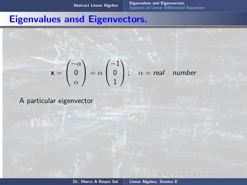
Abstract Linear AlgebraEigenvalues and Eigenvectors.Systems of Linear Differential Equations
Eigenvalues ansd Eigenvectors.
x =
−α0α
= α
−101
; α = real number
A particular eigenvector
is given by
x(1) =
−101
Dr. Marco A Roque Sol Linear Algebra. Session 8

Abstract Linear AlgebraEigenvalues and Eigenvectors.Systems of Linear Differential Equations
Eigenvalues ansd Eigenvectors.
x =
−α0α
= α
−101
; α = real number
A particular eigenvector is given by
x(1) =
−101
Dr. Marco A Roque Sol Linear Algebra. Session 8

Abstract Linear AlgebraEigenvalues and Eigenvectors.Systems of Linear Differential Equations
Eigenvalues ansd Eigenvectors.
x =
−α0α
= α
−101
; α = real number
A particular eigenvector is given by
x(1) =
−101
Dr. Marco A Roque Sol Linear Algebra. Session 8

Abstract Linear AlgebraEigenvalues and Eigenvectors.Systems of Linear Differential Equations
Eigenvalues ansd Eigenvectors.
Thus, the three linearly independent eigenvectors, are
x(1) =
110
x(2) =
101
x(3) =
− 101
and the matrix A, is Non-defective.
Dr. Marco A Roque Sol Linear Algebra. Session 8

Abstract Linear AlgebraEigenvalues and Eigenvectors.Systems of Linear Differential Equations
Eigenvalues ansd Eigenvectors.
Thus, the three linearly independent eigenvectors, are
x(1) =
110
x(2) =
101
x(3) =
− 101
and the matrix A, is Non-defective.
Dr. Marco A Roque Sol Linear Algebra. Session 8

Abstract Linear AlgebraEigenvalues and Eigenvectors.Systems of Linear Differential Equations
Eigenvalues ansd Eigenvectors.
Thus,
the three linearly independent eigenvectors, are
x(1) =
110
x(2) =
101
x(3) =
− 101
and the matrix A, is Non-defective.
Dr. Marco A Roque Sol Linear Algebra. Session 8

Abstract Linear AlgebraEigenvalues and Eigenvectors.Systems of Linear Differential Equations
Eigenvalues ansd Eigenvectors.
Thus, the three linearly independent
eigenvectors, are
x(1) =
110
x(2) =
101
x(3) =
− 101
and the matrix A, is Non-defective.
Dr. Marco A Roque Sol Linear Algebra. Session 8

Abstract Linear AlgebraEigenvalues and Eigenvectors.Systems of Linear Differential Equations
Eigenvalues ansd Eigenvectors.
Thus, the three linearly independent eigenvectors, are
x(1) =
110
x(2) =
101
x(3) =
− 101
and the matrix A, is Non-defective.
Dr. Marco A Roque Sol Linear Algebra. Session 8

Abstract Linear AlgebraEigenvalues and Eigenvectors.Systems of Linear Differential Equations
Eigenvalues ansd Eigenvectors.
Thus, the three linearly independent eigenvectors, are
x(1) =
110
x(2) =
101
x(3) =
− 101
and the matrix A, is Non-defective.
Dr. Marco A Roque Sol Linear Algebra. Session 8

Abstract Linear AlgebraEigenvalues and Eigenvectors.Systems of Linear Differential Equations
Eigenvalues ansd Eigenvectors.
Thus, the three linearly independent eigenvectors, are
x(1) =
110
x(2) =
101
x(3) =
− 101
and the matrix A, is Non-defective.
Dr. Marco A Roque Sol Linear Algebra. Session 8

Abstract Linear AlgebraEigenvalues and Eigenvectors.Systems of Linear Differential Equations
Eigenvalues ansd Eigenvectors.
Thus, the three linearly independent eigenvectors, are
x(1) =
110
x(2) =
101
x(3) =
− 101
and the matrix A, is Non-defective.
Dr. Marco A Roque Sol Linear Algebra. Session 8

Abstract Linear AlgebraEigenvalues and Eigenvectors.Systems of Linear Differential Equations
Eigenvalues ansd Eigenvectors.
Thus, the three linearly independent eigenvectors, are
x(1) =
110
x(2) =
101
x(3) =
− 101
and the matrix A, is Non-defective.
Dr. Marco A Roque Sol Linear Algebra. Session 8

Abstract Linear AlgebraEigenvalues and Eigenvectors.Systems of Linear Differential Equations
Eigenvalues and Eigenvectors.
Example 9.2
Find the eigenvalues and eigenvectors of the matrix
A =
0 1 11 0 11 1 0
Solution
The eigenvalues λ and eigenvectors x satisfy the equation(A− λI) x = 0, or
Dr. Marco A Roque Sol Linear Algebra. Session 8

Abstract Linear AlgebraEigenvalues and Eigenvectors.Systems of Linear Differential Equations
Eigenvalues and Eigenvectors.
Example 9.2
Find the eigenvalues and eigenvectors of the matrix
A =
0 1 11 0 11 1 0
Solution
The eigenvalues λ and eigenvectors x satisfy the equation(A− λI) x = 0, or
Dr. Marco A Roque Sol Linear Algebra. Session 8
Abstract Linear AlgebraEigenvalues and Eigenvectors.Systems of Linear Differential Equations
Eigenvalues and Eigenvectors.
Example 9.2
Find
the eigenvalues and eigenvectors of the matrix
A =
0 1 11 0 11 1 0
Solution
The eigenvalues λ and eigenvectors x satisfy the equation(A− λI) x = 0, or
Dr. Marco A Roque Sol Linear Algebra. Session 8
Abstract Linear AlgebraEigenvalues and Eigenvectors.Systems of Linear Differential Equations
Eigenvalues and Eigenvectors.
Example 9.2
Find the eigenvalues and
eigenvectors of the matrix
A =
0 1 11 0 11 1 0
Solution
The eigenvalues λ and eigenvectors x satisfy the equation(A− λI) x = 0, or
Dr. Marco A Roque Sol Linear Algebra. Session 8
Abstract Linear AlgebraEigenvalues and Eigenvectors.Systems of Linear Differential Equations
Eigenvalues and Eigenvectors.
Example 9.2
Find the eigenvalues and eigenvectors
of the matrix
A =
0 1 11 0 11 1 0
Solution
The eigenvalues λ and eigenvectors x satisfy the equation(A− λI) x = 0, or
Dr. Marco A Roque Sol Linear Algebra. Session 8

Abstract Linear AlgebraEigenvalues and Eigenvectors.Systems of Linear Differential Equations
Eigenvalues and Eigenvectors.
Example 9.2
Find the eigenvalues and eigenvectors of the matrix
A =
0 1 11 0 11 1 0
Solution
The eigenvalues λ and eigenvectors x satisfy the equation(A− λI) x = 0, or
Dr. Marco A Roque Sol Linear Algebra. Session 8
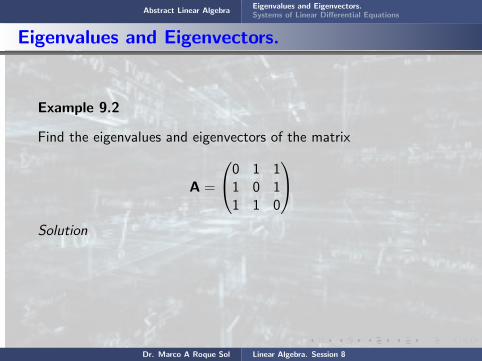

Abstract Linear AlgebraEigenvalues and Eigenvectors.Systems of Linear Differential Equations
Eigenvalues and Eigenvectors.
Example 9.2
Find the eigenvalues and eigenvectors of the matrix
A =
0 1 11 0 11 1 0
Solution
The eigenvalues λ and
eigenvectors x satisfy the equation(A− λI) x = 0, or
Dr. Marco A Roque Sol Linear Algebra. Session 8

Abstract Linear AlgebraEigenvalues and Eigenvectors.Systems of Linear Differential Equations
Eigenvalues and Eigenvectors.
Example 9.2
Find the eigenvalues and eigenvectors of the matrix
A =
0 1 11 0 11 1 0
Solution
The eigenvalues λ and
eigenvectors x satisfy the equation(A− λI) x = 0, or
Dr. Marco A Roque Sol Linear Algebra. Session 8
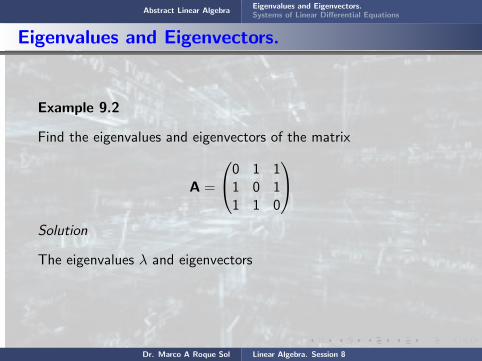
Abstract Linear AlgebraEigenvalues and Eigenvectors.Systems of Linear Differential Equations
Eigenvalues and Eigenvectors.
Example 9.2
Find the eigenvalues and eigenvectors of the matrix
A =
0 1 11 0 11 1 0
Solution
The eigenvalues λ and eigenvectors
x satisfy the equation(A− λI) x = 0, or
Dr. Marco A Roque Sol Linear Algebra. Session 8

Abstract Linear AlgebraEigenvalues and Eigenvectors.Systems of Linear Differential Equations
Eigenvalues and Eigenvectors.
Example 9.2
Find the eigenvalues and eigenvectors of the matrix
A =
0 1 11 0 11 1 0
Solution
The eigenvalues λ and eigenvectors x
satisfy the equation(A− λI) x = 0, or
Dr. Marco A Roque Sol Linear Algebra. Session 8

Abstract Linear AlgebraEigenvalues and Eigenvectors.Systems of Linear Differential Equations
Eigenvalues and Eigenvectors.
Example 9.2
Find the eigenvalues and eigenvectors of the matrix
A =
0 1 11 0 11 1 0
Solution
The eigenvalues λ and eigenvectors x satisfy the equation
(A− λI) x = 0, or
Dr. Marco A Roque Sol Linear Algebra. Session 8

Abstract Linear AlgebraEigenvalues and Eigenvectors.Systems of Linear Differential Equations
Eigenvalues and Eigenvectors.
Example 9.2
Find the eigenvalues and eigenvectors of the matrix
A =
0 1 11 0 11 1 0
Solution
The eigenvalues λ and eigenvectors x satisfy the equation(A− λI) x = 0, or
Dr. Marco A Roque Sol Linear Algebra. Session 8

Abstract Linear AlgebraEigenvalues and Eigenvectors.Systems of Linear Differential Equations
Eigenvalues and Eigenvectors.
(A− λI) x =
−λ 1 11 −λ 11 1 −λ
x1x2x3
=
000
The eigenvalues are the roots of the equation
|A− λI| =
∣∣∣∣∣∣−λ 1 11 −λ 11 1 −λ
∣∣∣∣∣∣ = −
∣∣∣∣∣∣1 −λ 1−λ 1 11 1 −λ
∣∣∣∣∣∣ =
∣∣∣∣∣∣1 −λ 11 1 −λ−λ 1 1
∣∣∣∣∣∣ =
∣∣∣∣∣∣1 −λ 10 λ+ 1 −1− λ0 −λ2 + 1 λ+ 1
∣∣∣∣∣∣ =
∣∣∣∣∣∣1 0 0−λ λ+ 1 −λ2 + 11 −1− λ λ+ 1
∣∣∣∣∣∣ =λ3 − 3λ− 2 = 0
Dr. Marco A Roque Sol Linear Algebra. Session 8

Abstract Linear AlgebraEigenvalues and Eigenvectors.Systems of Linear Differential Equations
Eigenvalues and Eigenvectors.
(A− λI) x =
−λ 1 11 −λ 11 1 −λ
x1x2x3
=
000
The eigenvalues
are the roots of the equation
|A− λI| =
∣∣∣∣∣∣−λ 1 11 −λ 11 1 −λ
∣∣∣∣∣∣ = −
∣∣∣∣∣∣1 −λ 1−λ 1 11 1 −λ
∣∣∣∣∣∣ =
∣∣∣∣∣∣1 −λ 11 1 −λ−λ 1 1
∣∣∣∣∣∣ =
∣∣∣∣∣∣1 −λ 10 λ+ 1 −1− λ0 −λ2 + 1 λ+ 1
∣∣∣∣∣∣ =
∣∣∣∣∣∣1 0 0−λ λ+ 1 −λ2 + 11 −1− λ λ+ 1
∣∣∣∣∣∣ =λ3 − 3λ− 2 = 0
Dr. Marco A Roque Sol Linear Algebra. Session 8

Abstract Linear AlgebraEigenvalues and Eigenvectors.Systems of Linear Differential Equations
Eigenvalues and Eigenvectors.
(A− λI) x =
−λ 1 11 −λ 11 1 −λ
x1x2x3
=
000
The eigenvalues are the roots
of the equation
|A− λI| =
∣∣∣∣∣∣−λ 1 11 −λ 11 1 −λ
∣∣∣∣∣∣ = −
∣∣∣∣∣∣1 −λ 1−λ 1 11 1 −λ
∣∣∣∣∣∣ =
∣∣∣∣∣∣1 −λ 11 1 −λ−λ 1 1
∣∣∣∣∣∣ =
∣∣∣∣∣∣1 −λ 10 λ+ 1 −1− λ0 −λ2 + 1 λ+ 1
∣∣∣∣∣∣ =
∣∣∣∣∣∣1 0 0−λ λ+ 1 −λ2 + 11 −1− λ λ+ 1
∣∣∣∣∣∣ =λ3 − 3λ− 2 = 0
Dr. Marco A Roque Sol Linear Algebra. Session 8
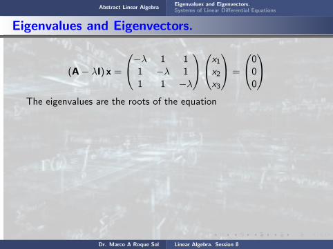
Abstract Linear AlgebraEigenvalues and Eigenvectors.Systems of Linear Differential Equations
Eigenvalues and Eigenvectors.
(A− λI) x =
−λ 1 11 −λ 11 1 −λ
x1x2x3
=
000
The eigenvalues are the roots of the equation
|A− λI| =
∣∣∣∣∣∣−λ 1 11 −λ 11 1 −λ
∣∣∣∣∣∣ = −
∣∣∣∣∣∣1 −λ 1−λ 1 11 1 −λ
∣∣∣∣∣∣ =
∣∣∣∣∣∣1 −λ 11 1 −λ−λ 1 1
∣∣∣∣∣∣ =
∣∣∣∣∣∣1 −λ 10 λ+ 1 −1− λ0 −λ2 + 1 λ+ 1
∣∣∣∣∣∣ =
∣∣∣∣∣∣1 0 0−λ λ+ 1 −λ2 + 11 −1− λ λ+ 1
∣∣∣∣∣∣ =λ3 − 3λ− 2 = 0
Dr. Marco A Roque Sol Linear Algebra. Session 8
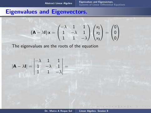
Abstract Linear AlgebraEigenvalues and Eigenvectors.Systems of Linear Differential Equations
Eigenvalues and Eigenvectors.
(A− λI) x =
−λ 1 11 −λ 11 1 −λ
x1x2x3
=
000
The eigenvalues are the roots of the equation
|A− λI| =
∣∣∣∣∣∣−λ 1 11 −λ 11 1 −λ
∣∣∣∣∣∣ =
−
∣∣∣∣∣∣1 −λ 1−λ 1 11 1 −λ
∣∣∣∣∣∣ =
∣∣∣∣∣∣1 −λ 11 1 −λ−λ 1 1
∣∣∣∣∣∣ =
∣∣∣∣∣∣1 −λ 10 λ+ 1 −1− λ0 −λ2 + 1 λ+ 1
∣∣∣∣∣∣ =
∣∣∣∣∣∣1 0 0−λ λ+ 1 −λ2 + 11 −1− λ λ+ 1
∣∣∣∣∣∣ =λ3 − 3λ− 2 = 0
Dr. Marco A Roque Sol Linear Algebra. Session 8
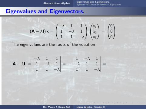
Abstract Linear AlgebraEigenvalues and Eigenvectors.Systems of Linear Differential Equations
Eigenvalues and Eigenvectors.
(A− λI) x =
−λ 1 11 −λ 11 1 −λ
x1x2x3
=
000
The eigenvalues are the roots of the equation
|A− λI| =
∣∣∣∣∣∣−λ 1 11 −λ 11 1 −λ
∣∣∣∣∣∣ = −
∣∣∣∣∣∣1 −λ 1−λ 1 11 1 −λ
∣∣∣∣∣∣ =
∣∣∣∣∣∣1 −λ 11 1 −λ−λ 1 1
∣∣∣∣∣∣ =
∣∣∣∣∣∣1 −λ 10 λ+ 1 −1− λ0 −λ2 + 1 λ+ 1
∣∣∣∣∣∣ =
∣∣∣∣∣∣1 0 0−λ λ+ 1 −λ2 + 11 −1− λ λ+ 1
∣∣∣∣∣∣ =λ3 − 3λ− 2 = 0
Dr. Marco A Roque Sol Linear Algebra. Session 8
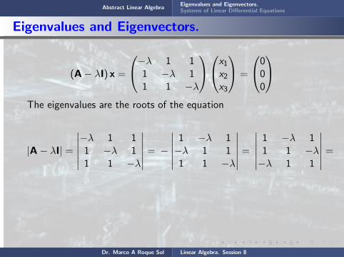
Abstract Linear AlgebraEigenvalues and Eigenvectors.Systems of Linear Differential Equations
Eigenvalues and Eigenvectors.
(A− λI) x =
−λ 1 11 −λ 11 1 −λ
x1x2x3
=
000
The eigenvalues are the roots of the equation
|A− λI| =
∣∣∣∣∣∣−λ 1 11 −λ 11 1 −λ
∣∣∣∣∣∣ = −
∣∣∣∣∣∣1 −λ 1−λ 1 11 1 −λ
∣∣∣∣∣∣ =
∣∣∣∣∣∣1 −λ 11 1 −λ−λ 1 1
∣∣∣∣∣∣ =
∣∣∣∣∣∣1 −λ 10 λ+ 1 −1− λ0 −λ2 + 1 λ+ 1
∣∣∣∣∣∣ =
∣∣∣∣∣∣1 0 0−λ λ+ 1 −λ2 + 11 −1− λ λ+ 1
∣∣∣∣∣∣ =
λ3 − 3λ− 2 = 0
Dr. Marco A Roque Sol Linear Algebra. Session 8
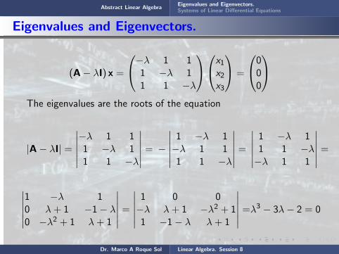
Abstract Linear AlgebraEigenvalues and Eigenvectors.Systems of Linear Differential Equations
Eigenvalues and Eigenvectors.
(A− λI) x =
−λ 1 11 −λ 11 1 −λ
x1x2x3
=
000
The eigenvalues are the roots of the equation
|A− λI| =
∣∣∣∣∣∣−λ 1 11 −λ 11 1 −λ
∣∣∣∣∣∣ = −
∣∣∣∣∣∣1 −λ 1−λ 1 11 1 −λ
∣∣∣∣∣∣ =
∣∣∣∣∣∣1 −λ 11 1 −λ−λ 1 1
∣∣∣∣∣∣ =
∣∣∣∣∣∣1 −λ 10 λ+ 1 −1− λ0 −λ2 + 1 λ+ 1
∣∣∣∣∣∣ =
∣∣∣∣∣∣1 0 0−λ λ+ 1 −λ2 + 11 −1− λ λ+ 1
∣∣∣∣∣∣ =λ3 − 3λ− 2 = 0
Dr. Marco A Roque Sol Linear Algebra. Session 8

Abstract Linear AlgebraEigenvalues and Eigenvectors.Systems of Linear Differential Equations
Eigenvalues and Eigenvectors.
The roots are λ1 = 2, λ2 = −1, and λ3 = −1 .
1) For λ1 = 2
−λ1 1 11 −λ1 11 1 −λ1
x1x2x3
=
−2 1 11 −2 11 1 −2
x1x2x3
=
000
We can reduce this to the equivalent system2 −1 −1
0 1 −10 0 0
x1x2x3
=
000
Dr. Marco A Roque Sol Linear Algebra. Session 8
Abstract Linear AlgebraEigenvalues and Eigenvectors.Systems of Linear Differential Equations
Eigenvalues and Eigenvectors.
The roots
are λ1 = 2, λ2 = −1, and λ3 = −1 .
1) For λ1 = 2
−λ1 1 11 −λ1 11 1 −λ1
x1x2x3
=
−2 1 11 −2 11 1 −2
x1x2x3
=
000
We can reduce this to the equivalent system2 −1 −1
0 1 −10 0 0
x1x2x3
=
000
Dr. Marco A Roque Sol Linear Algebra. Session 8

Abstract Linear AlgebraEigenvalues and Eigenvectors.Systems of Linear Differential Equations
Eigenvalues and Eigenvectors.
The roots are λ1 = 2, λ2 = −1, and λ3 = −1 .
1) For λ1 = 2
−λ1 1 11 −λ1 11 1 −λ1
x1x2x3
=
−2 1 11 −2 11 1 −2
x1x2x3
=
000
We can reduce this to the equivalent system2 −1 −1
0 1 −10 0 0
x1x2x3
=
000
Dr. Marco A Roque Sol Linear Algebra. Session 8

Abstract Linear AlgebraEigenvalues and Eigenvectors.Systems of Linear Differential Equations
Eigenvalues and Eigenvectors.
The roots are λ1 = 2, λ2 = −1, and λ3 = −1 .
1) For λ1 = 2
−λ1 1 11 −λ1 11 1 −λ1
x1x2x3
=
−2 1 11 −2 11 1 −2
x1x2x3
=
000
We can reduce this to the equivalent system2 −1 −10 1 −10 0 0
x1x2x3
=
000
Dr. Marco A Roque Sol Linear Algebra. Session 8
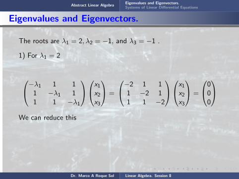
Abstract Linear AlgebraEigenvalues and Eigenvectors.Systems of Linear Differential Equations
Eigenvalues and Eigenvectors.
The roots are λ1 = 2, λ2 = −1, and λ3 = −1 .
1) For λ1 = 2
−λ1 1 11 −λ1 11 1 −λ1
x1x2x3
=
−2 1 11 −2 11 1 −2
x1x2x3
=
000
We can reduce this
to the equivalent system2 −1 −10 1 −10 0 0
x1x2x3
=
000
Dr. Marco A Roque Sol Linear Algebra. Session 8

Abstract Linear AlgebraEigenvalues and Eigenvectors.Systems of Linear Differential Equations
Eigenvalues and Eigenvectors.
The roots are λ1 = 2, λ2 = −1, and λ3 = −1 .
1) For λ1 = 2
−λ1 1 11 −λ1 11 1 −λ1
x1x2x3
=
−2 1 11 −2 11 1 −2
x1x2x3
=
000
We can reduce this to the equivalent system
2 −1 −10 1 −10 0 0
x1x2x3
=
000
Dr. Marco A Roque Sol Linear Algebra. Session 8

Abstract Linear AlgebraEigenvalues and Eigenvectors.Systems of Linear Differential Equations
Eigenvalues and Eigenvectors.
The roots are λ1 = 2, λ2 = −1, and λ3 = −1 .
1) For λ1 = 2
−λ1 1 11 −λ1 11 1 −λ1
x1x2x3
=
−2 1 11 −2 11 1 −2
x1x2x3
=
000
We can reduce this to the equivalent system2 −1 −1
0 1 −10 0 0
x1x2x3
=
000
Dr. Marco A Roque Sol Linear Algebra. Session 8

Abstract Linear AlgebraEigenvalues and Eigenvectors.Systems of Linear Differential Equations
Eigenvalues and Eigenvectors.
The above system is reduced immediately to the equations
2x1 − x2 − x3 = 0 x2 − x3 = 0
Two equations and three unknowns. Hence, one of them is a freevariable, let’s say x3 = α. Therefore x2 = x3 = α andx1 = (x2 + x3)/2 = α. Thus we have
x =
ααα
= α
111
; α = real number
Dr. Marco A Roque Sol Linear Algebra. Session 8
Abstract Linear AlgebraEigenvalues and Eigenvectors.Systems of Linear Differential Equations
Eigenvalues and Eigenvectors.
The above system
is reduced immediately to the equations
2x1 − x2 − x3 = 0 x2 − x3 = 0
Two equations and three unknowns. Hence, one of them is a freevariable, let’s say x3 = α. Therefore x2 = x3 = α andx1 = (x2 + x3)/2 = α. Thus we have
x =
ααα
= α
111
; α = real number
Dr. Marco A Roque Sol Linear Algebra. Session 8

Abstract Linear AlgebraEigenvalues and Eigenvectors.Systems of Linear Differential Equations
Eigenvalues and Eigenvectors.
The above system is reduced
immediately to the equations
2x1 − x2 − x3 = 0 x2 − x3 = 0
Two equations and three unknowns. Hence, one of them is a freevariable, let’s say x3 = α. Therefore x2 = x3 = α andx1 = (x2 + x3)/2 = α. Thus we have
x =
ααα
= α
111
; α = real number
Dr. Marco A Roque Sol Linear Algebra. Session 8

Abstract Linear AlgebraEigenvalues and Eigenvectors.Systems of Linear Differential Equations
Eigenvalues and Eigenvectors.
The above system is reduced immediately to
the equations
2x1 − x2 − x3 = 0 x2 − x3 = 0
Two equations and three unknowns. Hence, one of them is a freevariable, let’s say x3 = α. Therefore x2 = x3 = α andx1 = (x2 + x3)/2 = α. Thus we have
x =
ααα
= α
111
; α = real number
Dr. Marco A Roque Sol Linear Algebra. Session 8

Abstract Linear AlgebraEigenvalues and Eigenvectors.Systems of Linear Differential Equations
Eigenvalues and Eigenvectors.
The above system is reduced immediately to the equations
2x1 − x2 − x3 = 0 x2 − x3 = 0
Two equations and three unknowns. Hence, one of them is a freevariable, let’s say x3 = α. Therefore x2 = x3 = α andx1 = (x2 + x3)/2 = α. Thus we have
x =
ααα
= α
111
; α = real number
Dr. Marco A Roque Sol Linear Algebra. Session 8
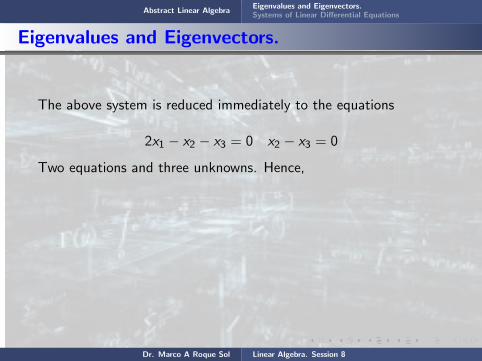
Abstract Linear AlgebraEigenvalues and Eigenvectors.Systems of Linear Differential Equations
Eigenvalues and Eigenvectors.
The above system is reduced immediately to the equations
2x1 − x2 − x3 = 0 x2 − x3 = 0
Two equations and three unknowns. Hence,
one of them is a freevariable, let’s say x3 = α. Therefore x2 = x3 = α andx1 = (x2 + x3)/2 = α. Thus we have
x =
ααα
= α
111
; α = real number
Dr. Marco A Roque Sol Linear Algebra. Session 8

Abstract Linear AlgebraEigenvalues and Eigenvectors.Systems of Linear Differential Equations
Eigenvalues and Eigenvectors.
The above system is reduced immediately to the equations
2x1 − x2 − x3 = 0 x2 − x3 = 0
Two equations and three unknowns. Hence, one of them is a freevariable,
let’s say x3 = α. Therefore x2 = x3 = α andx1 = (x2 + x3)/2 = α. Thus we have
x =
ααα
= α
111
; α = real number
Dr. Marco A Roque Sol Linear Algebra. Session 8

Abstract Linear AlgebraEigenvalues and Eigenvectors.Systems of Linear Differential Equations
Eigenvalues and Eigenvectors.
The above system is reduced immediately to the equations
2x1 − x2 − x3 = 0 x2 − x3 = 0
Two equations and three unknowns. Hence, one of them is a freevariable, let’s say x3 = α. Therefore
x2 = x3 = α andx1 = (x2 + x3)/2 = α. Thus we have
x =
ααα
= α
111
; α = real number
Dr. Marco A Roque Sol Linear Algebra. Session 8

Abstract Linear AlgebraEigenvalues and Eigenvectors.Systems of Linear Differential Equations
Eigenvalues and Eigenvectors.
The above system is reduced immediately to the equations
2x1 − x2 − x3 = 0 x2 − x3 = 0
Two equations and three unknowns. Hence, one of them is a freevariable, let’s say x3 = α. Therefore x2 = x3 = α andx1 = (x2 + x3)/2 = α.
Thus we have
x =
ααα
= α
111
; α = real number
Dr. Marco A Roque Sol Linear Algebra. Session 8

Abstract Linear AlgebraEigenvalues and Eigenvectors.Systems of Linear Differential Equations
Eigenvalues and Eigenvectors.
The above system is reduced immediately to the equations
2x1 − x2 − x3 = 0 x2 − x3 = 0
Two equations and three unknowns. Hence, one of them is a freevariable, let’s say x3 = α. Therefore x2 = x3 = α andx1 = (x2 + x3)/2 = α. Thus we have
x =
ααα
= α
111
; α = real number
Dr. Marco A Roque Sol Linear Algebra. Session 8

Abstract Linear AlgebraEigenvalues and Eigenvectors.Systems of Linear Differential Equations
Eigenvalues and Eigenvectors.
The above system is reduced immediately to the equations
2x1 − x2 − x3 = 0 x2 − x3 = 0
Two equations and three unknowns. Hence, one of them is a freevariable, let’s say x3 = α. Therefore x2 = x3 = α andx1 = (x2 + x3)/2 = α. Thus we have
x =
ααα
= α
111
; α = real number
Dr. Marco A Roque Sol Linear Algebra. Session 8

Abstract Linear AlgebraEigenvalues and Eigenvectors.Systems of Linear Differential Equations
Eigenvalues and Eigenvectors.
In particular, we have the eigenvector
x(1) =
111
2) For λ2 = −1
−λ2 1 11 −λ2 11 1 −λ2
x1x2x3
=
1 1 11 1 11 1 1
x1x2x3
=
000
Dr. Marco A Roque Sol Linear Algebra. Session 8

Abstract Linear AlgebraEigenvalues and Eigenvectors.Systems of Linear Differential Equations
Eigenvalues and Eigenvectors.
In particular,
we have the eigenvector
x(1) =
111
2) For λ2 = −1
−λ2 1 11 −λ2 11 1 −λ2
x1x2x3
=
1 1 11 1 11 1 1
x1x2x3
=
000
Dr. Marco A Roque Sol Linear Algebra. Session 8

Abstract Linear AlgebraEigenvalues and Eigenvectors.Systems of Linear Differential Equations
Eigenvalues and Eigenvectors.
In particular, we have
the eigenvector
x(1) =
111
2) For λ2 = −1
−λ2 1 11 −λ2 11 1 −λ2
x1x2x3
=
1 1 11 1 11 1 1
x1x2x3
=
000
Dr. Marco A Roque Sol Linear Algebra. Session 8
Abstract Linear AlgebraEigenvalues and Eigenvectors.Systems of Linear Differential Equations
Eigenvalues and Eigenvectors.
In particular, we have the eigenvector
x(1) =
111
2) For λ2 = −1
−λ2 1 11 −λ2 11 1 −λ2
x1x2x3
=
1 1 11 1 11 1 1
x1x2x3
=
000
Dr. Marco A Roque Sol Linear Algebra. Session 8

Abstract Linear AlgebraEigenvalues and Eigenvectors.Systems of Linear Differential Equations
Eigenvalues and Eigenvectors.
In particular, we have the eigenvector
x(1) =
111
2) For λ2 = −1
−λ2 1 11 −λ2 11 1 −λ2
x1x2x3
=
1 1 11 1 11 1 1
x1x2x3
=
000
Dr. Marco A Roque Sol Linear Algebra. Session 8

Abstract Linear AlgebraEigenvalues and Eigenvectors.Systems of Linear Differential Equations
Eigenvalues and Eigenvectors.
In particular, we have the eigenvector
x(1) =
111
2) For λ2 = −1
−λ2 1 11 −λ2 11 1 −λ2
x1x2x3
=
1 1 11 1 11 1 1
x1x2x3
=
000
Dr. Marco A Roque Sol Linear Algebra. Session 8

Abstract Linear AlgebraEigenvalues and Eigenvectors.Systems of Linear Differential Equations
Eigenvalues and Eigenvectors.
In particular, we have the eigenvector
x(1) =
111
2) For λ2 = −1
−λ2 1 11 −λ2 11 1 −λ2
x1x2x3
=
1 1 11 1 11 1 1
x1x2x3
=
000
Dr. Marco A Roque Sol Linear Algebra. Session 8

Abstract Linear AlgebraEigenvalues and Eigenvectors.Systems of Linear Differential Equations
Eigenvalues and Eigenvectors.
In particular, we have the eigenvector
x(1) =
111
2) For λ2 = −1
−λ2 1 11 −λ2 11 1 −λ2
x1x2x3
=
1 1 11 1 11 1 1
x1x2x3
=
000
Dr. Marco A Roque Sol Linear Algebra. Session 8

Abstract Linear AlgebraEigenvalues and Eigenvectors.Systems of Linear Differential Equations
Eigenvalues and Eigenvectors.
The above system is reduced immediately to the single equation
x1 + x2 + x3 = 0
One equation and three unknowns. Hence, two of them are freeveriables, let’s say x1 = α, x2 = β, and x3 = −α− β . Thus wehave
x =
αβ
−α− β
= α
10−1
+ β
01−1
; α, β = real numbers
Dr. Marco A Roque Sol Linear Algebra. Session 8
Abstract Linear AlgebraEigenvalues and Eigenvectors.Systems of Linear Differential Equations
Eigenvalues and Eigenvectors.
The above system
is reduced immediately to the single equation
x1 + x2 + x3 = 0
One equation and three unknowns. Hence, two of them are freeveriables, let’s say x1 = α, x2 = β, and x3 = −α− β . Thus wehave
x =
αβ
−α− β
= α
10−1
+ β
01−1
; α, β = real numbers
Dr. Marco A Roque Sol Linear Algebra. Session 8
Abstract Linear AlgebraEigenvalues and Eigenvectors.Systems of Linear Differential Equations
Eigenvalues and Eigenvectors.
The above system is reduced
immediately to the single equation
x1 + x2 + x3 = 0
One equation and three unknowns. Hence, two of them are freeveriables, let’s say x1 = α, x2 = β, and x3 = −α− β . Thus wehave
x =
αβ
−α− β
= α
10−1
+ β
01−1
; α, β = real numbers
Dr. Marco A Roque Sol Linear Algebra. Session 8
Abstract Linear AlgebraEigenvalues and Eigenvectors.Systems of Linear Differential Equations
Eigenvalues and Eigenvectors.
The above system is reduced immediately to
the single equation
x1 + x2 + x3 = 0
One equation and three unknowns. Hence, two of them are freeveriables, let’s say x1 = α, x2 = β, and x3 = −α− β . Thus wehave
x =
αβ
−α− β
= α
10−1
+ β
01−1
; α, β = real numbers
Dr. Marco A Roque Sol Linear Algebra. Session 8

Abstract Linear AlgebraEigenvalues and Eigenvectors.Systems of Linear Differential Equations
Eigenvalues and Eigenvectors.
The above system is reduced immediately to the single equation
x1 + x2 + x3 = 0
One equation and three unknowns. Hence, two of them are freeveriables, let’s say x1 = α, x2 = β, and x3 = −α− β . Thus wehave
x =
αβ
−α− β
= α
10−1
+ β
01−1
; α, β = real numbers
Dr. Marco A Roque Sol Linear Algebra. Session 8

Abstract Linear AlgebraEigenvalues and Eigenvectors.Systems of Linear Differential Equations
Eigenvalues and Eigenvectors.
The above system is reduced immediately to the single equation
x1 + x2 + x3 = 0
One equation and
three unknowns. Hence, two of them are freeveriables, let’s say x1 = α, x2 = β, and x3 = −α− β . Thus wehave
x =
αβ
−α− β
= α
10−1
+ β
01−1
; α, β = real numbers
Dr. Marco A Roque Sol Linear Algebra. Session 8
Abstract Linear AlgebraEigenvalues and Eigenvectors.Systems of Linear Differential Equations
Eigenvalues and Eigenvectors.
The above system is reduced immediately to the single equation
x1 + x2 + x3 = 0
One equation and three unknowns.
Hence, two of them are freeveriables, let’s say x1 = α, x2 = β, and x3 = −α− β . Thus wehave
x =
αβ
−α− β
= α
10−1
+ β
01−1
; α, β = real numbers
Dr. Marco A Roque Sol Linear Algebra. Session 8

Abstract Linear AlgebraEigenvalues and Eigenvectors.Systems of Linear Differential Equations
Eigenvalues and Eigenvectors.
The above system is reduced immediately to the single equation
x1 + x2 + x3 = 0
One equation and three unknowns. Hence,
two of them are freeveriables, let’s say x1 = α, x2 = β, and x3 = −α− β . Thus wehave
x =
αβ
−α− β
= α
10−1
+ β
01−1
; α, β = real numbers
Dr. Marco A Roque Sol Linear Algebra. Session 8

Abstract Linear AlgebraEigenvalues and Eigenvectors.Systems of Linear Differential Equations
Eigenvalues and Eigenvectors.
The above system is reduced immediately to the single equation
x1 + x2 + x3 = 0
One equation and three unknowns. Hence, two of them
are freeveriables, let’s say x1 = α, x2 = β, and x3 = −α− β . Thus wehave
x =
αβ
−α− β
= α
10−1
+ β
01−1
; α, β = real numbers
Dr. Marco A Roque Sol Linear Algebra. Session 8

Abstract Linear AlgebraEigenvalues and Eigenvectors.Systems of Linear Differential Equations
Eigenvalues and Eigenvectors.
The above system is reduced immediately to the single equation
x1 + x2 + x3 = 0
One equation and three unknowns. Hence, two of them are freeveriables,
let’s say x1 = α, x2 = β, and x3 = −α− β . Thus wehave
x =
αβ
−α− β
= α
10−1
+ β
01−1
; α, β = real numbers
Dr. Marco A Roque Sol Linear Algebra. Session 8

Abstract Linear AlgebraEigenvalues and Eigenvectors.Systems of Linear Differential Equations
Eigenvalues and Eigenvectors.
The above system is reduced immediately to the single equation
x1 + x2 + x3 = 0
One equation and three unknowns. Hence, two of them are freeveriables, let’s say
x1 = α, x2 = β, and x3 = −α− β . Thus wehave
x =
αβ
−α− β
= α
10−1
+ β
01−1
; α, β = real numbers
Dr. Marco A Roque Sol Linear Algebra. Session 8
Abstract Linear AlgebraEigenvalues and Eigenvectors.Systems of Linear Differential Equations
Eigenvalues and Eigenvectors.
The above system is reduced immediately to the single equation
x1 + x2 + x3 = 0
One equation and three unknowns. Hence, two of them are freeveriables, let’s say x1 = α,
x2 = β, and x3 = −α− β . Thus wehave
x =
αβ
−α− β
= α
10−1
+ β
01−1
; α, β = real numbers
Dr. Marco A Roque Sol Linear Algebra. Session 8
Abstract Linear AlgebraEigenvalues and Eigenvectors.Systems of Linear Differential Equations
Eigenvalues and Eigenvectors.
The above system is reduced immediately to the single equation
x1 + x2 + x3 = 0
One equation and three unknowns. Hence, two of them are freeveriables, let’s say x1 = α, x2 = β, and
x3 = −α− β . Thus wehave
x =
αβ
−α− β
= α
10−1
+ β
01−1
; α, β = real numbers
Dr. Marco A Roque Sol Linear Algebra. Session 8
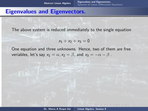
Abstract Linear AlgebraEigenvalues and Eigenvectors.Systems of Linear Differential Equations
Eigenvalues and Eigenvectors.
The above system is reduced immediately to the single equation
x1 + x2 + x3 = 0
One equation and three unknowns. Hence, two of them are freeveriables, let’s say x1 = α, x2 = β, and x3 = −α− β .
Thus wehave
x =
αβ
−α− β
= α
10−1
+ β
01−1
; α, β = real numbers
Dr. Marco A Roque Sol Linear Algebra. Session 8
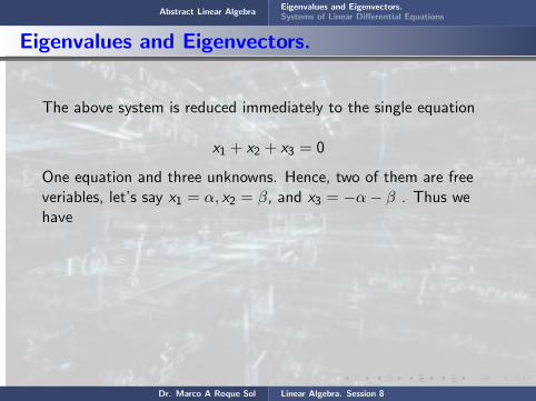
Abstract Linear AlgebraEigenvalues and Eigenvectors.Systems of Linear Differential Equations
Eigenvalues and Eigenvectors.
The above system is reduced immediately to the single equation
x1 + x2 + x3 = 0
One equation and three unknowns. Hence, two of them are freeveriables, let’s say x1 = α, x2 = β, and x3 = −α− β . Thus wehave
x =
αβ
−α− β
= α
10−1
+ β
01−1
; α, β = real numbers
Dr. Marco A Roque Sol Linear Algebra. Session 8
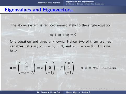
Abstract Linear AlgebraEigenvalues and Eigenvectors.Systems of Linear Differential Equations
Eigenvalues and Eigenvectors.
The above system is reduced immediately to the single equation
x1 + x2 + x3 = 0
One equation and three unknowns. Hence, two of them are freeveriables, let’s say x1 = α, x2 = β, and x3 = −α− β . Thus wehave
x =
αβ
−α− β
= α
10−1
+ β
01−1
; α, β = real numbers
Dr. Marco A Roque Sol Linear Algebra. Session 8

Abstract Linear AlgebraEigenvalues and Eigenvectors.Systems of Linear Differential Equations
Eigenvalues and Eigenvectors.
In this way two linearly independent eigenvectors associated toλ2 = −1 are ( α = β = 1 )
x(2) =
10
− 1
x(3) =
01
− 1
Thus, the three linearly independent eigenvectors, are
x(1) =
111
x(2) =
10
− 1
x(3) =
01
− 1
that is, the matrix A is Nondefective
Dr. Marco A Roque Sol Linear Algebra. Session 8

Abstract Linear AlgebraEigenvalues and Eigenvectors.Systems of Linear Differential Equations
Eigenvalues and Eigenvectors.
In this way
two linearly independent eigenvectors associated toλ2 = −1 are ( α = β = 1 )
x(2) =
10
− 1
x(3) =
01
− 1
Thus, the three linearly independent eigenvectors, are
x(1) =
111
x(2) =
10
− 1
x(3) =
01
− 1
that is, the matrix A is Nondefective
Dr. Marco A Roque Sol Linear Algebra. Session 8

Abstract Linear AlgebraEigenvalues and Eigenvectors.Systems of Linear Differential Equations
Eigenvalues and Eigenvectors.
In this way two linearly
independent eigenvectors associated toλ2 = −1 are ( α = β = 1 )
x(2) =
10
− 1
x(3) =
01
− 1
Thus, the three linearly independent eigenvectors, are
x(1) =
111
x(2) =
10
− 1
x(3) =
01
− 1
that is, the matrix A is Nondefective
Dr. Marco A Roque Sol Linear Algebra. Session 8

Abstract Linear AlgebraEigenvalues and Eigenvectors.Systems of Linear Differential Equations
Eigenvalues and Eigenvectors.
In this way two linearly independent eigenvectors
associated toλ2 = −1 are ( α = β = 1 )
x(2) =
10
− 1
x(3) =
01
− 1
Thus, the three linearly independent eigenvectors, are
x(1) =
111
x(2) =
10
− 1
x(3) =
01
− 1
that is, the matrix A is Nondefective
Dr. Marco A Roque Sol Linear Algebra. Session 8

Abstract Linear AlgebraEigenvalues and Eigenvectors.Systems of Linear Differential Equations
Eigenvalues and Eigenvectors.
In this way two linearly independent eigenvectors associated toλ2 = −1 are
( α = β = 1 )
x(2) =
10
− 1
x(3) =
01
− 1
Thus, the three linearly independent eigenvectors, are
x(1) =
111
x(2) =
10
− 1
x(3) =
01
− 1
that is, the matrix A is Nondefective
Dr. Marco A Roque Sol Linear Algebra. Session 8

Abstract Linear AlgebraEigenvalues and Eigenvectors.Systems of Linear Differential Equations
Eigenvalues and Eigenvectors.
In this way two linearly independent eigenvectors associated toλ2 = −1 are ( α = β = 1 )
x(2) =
10
− 1
x(3) =
01
− 1
Thus, the three linearly independent eigenvectors, are
x(1) =
111
x(2) =
10
− 1
x(3) =
01
− 1
that is, the matrix A is Nondefective
Dr. Marco A Roque Sol Linear Algebra. Session 8

Abstract Linear AlgebraEigenvalues and Eigenvectors.Systems of Linear Differential Equations
Eigenvalues and Eigenvectors.
In this way two linearly independent eigenvectors associated toλ2 = −1 are ( α = β = 1 )
x(2) =
10
− 1
x(3) =
01
− 1
Thus, the three linearly independent eigenvectors, are
x(1) =
111
x(2) =
10
− 1
x(3) =
01
− 1
that is, the matrix A is Nondefective
Dr. Marco A Roque Sol Linear Algebra. Session 8
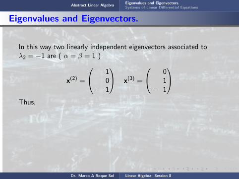
Abstract Linear AlgebraEigenvalues and Eigenvectors.Systems of Linear Differential Equations
Eigenvalues and Eigenvectors.
In this way two linearly independent eigenvectors associated toλ2 = −1 are ( α = β = 1 )
x(2) =
10
− 1
x(3) =
01
− 1
Thus,
the three linearly independent eigenvectors, are
x(1) =
111
x(2) =
10
− 1
x(3) =
01
− 1
that is, the matrix A is Nondefective
Dr. Marco A Roque Sol Linear Algebra. Session 8

Abstract Linear AlgebraEigenvalues and Eigenvectors.Systems of Linear Differential Equations
Eigenvalues and Eigenvectors.
In this way two linearly independent eigenvectors associated toλ2 = −1 are ( α = β = 1 )
x(2) =
10
− 1
x(3) =
01
− 1
Thus, the three
linearly independent eigenvectors, are
x(1) =
111
x(2) =
10
− 1
x(3) =
01
− 1
that is, the matrix A is Nondefective
Dr. Marco A Roque Sol Linear Algebra. Session 8

Abstract Linear AlgebraEigenvalues and Eigenvectors.Systems of Linear Differential Equations
Eigenvalues and Eigenvectors.
In this way two linearly independent eigenvectors associated toλ2 = −1 are ( α = β = 1 )
x(2) =
10
− 1
x(3) =
01
− 1
Thus, the three linearly independent
eigenvectors, are
x(1) =
111
x(2) =
10
− 1
x(3) =
01
− 1
that is, the matrix A is Nondefective
Dr. Marco A Roque Sol Linear Algebra. Session 8

Abstract Linear AlgebraEigenvalues and Eigenvectors.Systems of Linear Differential Equations
Eigenvalues and Eigenvectors.
In this way two linearly independent eigenvectors associated toλ2 = −1 are ( α = β = 1 )
x(2) =
10
− 1
x(3) =
01
− 1
Thus, the three linearly independent eigenvectors, are
x(1) =
111
x(2) =
10
− 1
x(3) =
01
− 1
that is, the matrix A is Nondefective
Dr. Marco A Roque Sol Linear Algebra. Session 8
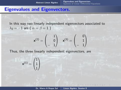
Abstract Linear AlgebraEigenvalues and Eigenvectors.Systems of Linear Differential Equations
Eigenvalues and Eigenvectors.
In this way two linearly independent eigenvectors associated toλ2 = −1 are ( α = β = 1 )
x(2) =
10
− 1
x(3) =
01
− 1
Thus, the three linearly independent eigenvectors, are
x(1) =
111
x(2) =
10
− 1
x(3) =
01
− 1
that is,
the matrix A is Nondefective
Dr. Marco A Roque Sol Linear Algebra. Session 8

Abstract Linear AlgebraEigenvalues and Eigenvectors.Systems of Linear Differential Equations
Eigenvalues and Eigenvectors.
In this way two linearly independent eigenvectors associated toλ2 = −1 are ( α = β = 1 )
x(2) =
10
− 1
x(3) =
01
− 1
Thus, the three linearly independent eigenvectors, are
x(1) =
111
x(2) =
10
− 1
x(3) =
01
− 1
that is, the matrix A
is Nondefective
Dr. Marco A Roque Sol Linear Algebra. Session 8
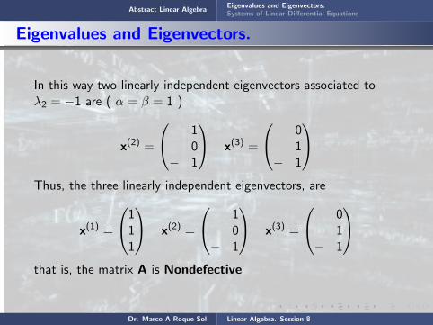
Abstract Linear AlgebraEigenvalues and Eigenvectors.Systems of Linear Differential Equations
Eigenvalues and Eigenvectors.
In this way two linearly independent eigenvectors associated toλ2 = −1 are ( α = β = 1 )
x(2) =
10
− 1
x(3) =
01
− 1
Thus, the three linearly independent eigenvectors, are
x(1) =
111
x(2) =
10
− 1
x(3) =
01
− 1
that is, the matrix A is Nondefective
Dr. Marco A Roque Sol Linear Algebra. Session 8

Abstract Linear AlgebraEigenvalues and Eigenvectors.Systems of Linear Differential Equations
Eigenvalues ansd Eigenvectors.
Example 9.3
Find the eigenvalues and eigenvectors of the matrix
A =
4 6 61 3 21 −5 −2
Solution
The eigenvalues λ and eigenvectors x satisfy the equation(A− λI) x = 0, or
Dr. Marco A Roque Sol Linear Algebra. Session 8

Abstract Linear AlgebraEigenvalues and Eigenvectors.Systems of Linear Differential Equations
Eigenvalues ansd Eigenvectors.
Example 9.3
Find
the eigenvalues and eigenvectors of the matrix
A =
4 6 61 3 21 −5 −2
Solution
The eigenvalues λ and eigenvectors x satisfy the equation(A− λI) x = 0, or
Dr. Marco A Roque Sol Linear Algebra. Session 8

Abstract Linear AlgebraEigenvalues and Eigenvectors.Systems of Linear Differential Equations
Eigenvalues ansd Eigenvectors.
Example 9.3
Find the eigenvalues and
eigenvectors of the matrix
A =
4 6 61 3 21 −5 −2
Solution
The eigenvalues λ and eigenvectors x satisfy the equation(A− λI) x = 0, or
Dr. Marco A Roque Sol Linear Algebra. Session 8

Abstract Linear AlgebraEigenvalues and Eigenvectors.Systems of Linear Differential Equations
Eigenvalues ansd Eigenvectors.
Example 9.3
Find the eigenvalues and eigenvectors of the matrix
A =
4 6 61 3 21 −5 −2
Solution
The eigenvalues λ and eigenvectors x satisfy the equation(A− λI) x = 0, or
Dr. Marco A Roque Sol Linear Algebra. Session 8

Abstract Linear AlgebraEigenvalues and Eigenvectors.Systems of Linear Differential Equations
Eigenvalues ansd Eigenvectors.
Example 9.3
Find the eigenvalues and eigenvectors of the matrix
A =
4 6 61 3 21 −5 −2
Solution
The eigenvalues λ and eigenvectors x satisfy the equation(A− λI) x = 0, or
Dr. Marco A Roque Sol Linear Algebra. Session 8
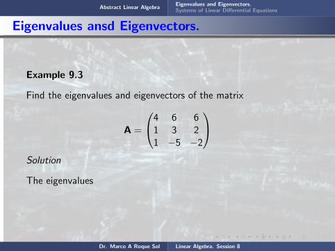
Abstract Linear AlgebraEigenvalues and Eigenvectors.Systems of Linear Differential Equations
Eigenvalues ansd Eigenvectors.
Example 9.3
Find the eigenvalues and eigenvectors of the matrix
A =
4 6 61 3 21 −5 −2
Solution
The eigenvalues
λ and eigenvectors x satisfy the equation(A− λI) x = 0, or
Dr. Marco A Roque Sol Linear Algebra. Session 8
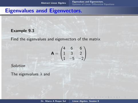
Abstract Linear AlgebraEigenvalues and Eigenvectors.Systems of Linear Differential Equations
Eigenvalues ansd Eigenvectors.
Example 9.3
Find the eigenvalues and eigenvectors of the matrix
A =
4 6 61 3 21 −5 −2
Solution
The eigenvalues λ and
eigenvectors x satisfy the equation(A− λI) x = 0, or
Dr. Marco A Roque Sol Linear Algebra. Session 8

Abstract Linear AlgebraEigenvalues and Eigenvectors.Systems of Linear Differential Equations
Eigenvalues ansd Eigenvectors.
Example 9.3
Find the eigenvalues and eigenvectors of the matrix
A =
4 6 61 3 21 −5 −2
Solution
The eigenvalues λ and eigenvectors x
satisfy the equation(A− λI) x = 0, or
Dr. Marco A Roque Sol Linear Algebra. Session 8

Abstract Linear AlgebraEigenvalues and Eigenvectors.Systems of Linear Differential Equations
Eigenvalues ansd Eigenvectors.
Example 9.3
Find the eigenvalues and eigenvectors of the matrix
A =
4 6 61 3 21 −5 −2
Solution
The eigenvalues λ and eigenvectors x satisfy the equation
(A− λI) x = 0, or
Dr. Marco A Roque Sol Linear Algebra. Session 8
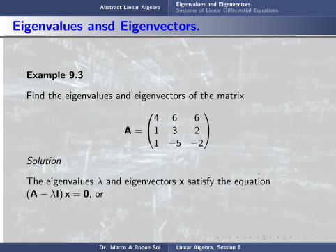
Abstract Linear AlgebraEigenvalues and Eigenvectors.Systems of Linear Differential Equations
Eigenvalues ansd Eigenvectors.
Example 9.3
Find the eigenvalues and eigenvectors of the matrix
A =
4 6 61 3 21 −5 −2
Solution
The eigenvalues λ and eigenvectors x satisfy the equation(A− λI) x = 0, or
Dr. Marco A Roque Sol Linear Algebra. Session 8

Abstract Linear AlgebraEigenvalues and Eigenvectors.Systems of Linear Differential Equations
Eigenvalues ansd Eigenvectors.
(A− λI) x =
4− λ 6 61 3− λ 2−1 −5 −2− λ
x1x2x3
=
000
The eigenvalues are the roots of the equation
|A− λI| =
∣∣∣∣∣∣4− λ 6 6
1 3− λ 2−1 −5 −2− λ
∣∣∣∣∣∣ =
∣∣∣∣∣∣4− λ 6 6
1 3− λ 20 −2− λ −λ
∣∣∣∣∣∣ =
−
∣∣∣∣∣∣1 3− λ 20 −(4− λ)(3− λ) + 6 6− 2(4− λ)0 −2− λ −λ
∣∣∣∣∣∣ = − λ3 + 5λ2 − 8λ+ 4 =
−(λ− 1)(λ− 2)2 = 0
Dr. Marco A Roque Sol Linear Algebra. Session 8
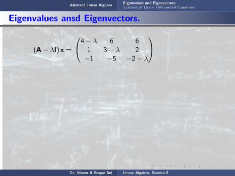
Abstract Linear AlgebraEigenvalues and Eigenvectors.Systems of Linear Differential Equations
Eigenvalues ansd Eigenvectors.
(A− λI) x =
4− λ 6 61 3− λ 2−1 −5 −2− λ
x1x2x3
=
000
The eigenvalues are the roots of the equation
|A− λI| =
∣∣∣∣∣∣4− λ 6 6
1 3− λ 2−1 −5 −2− λ
∣∣∣∣∣∣ =
∣∣∣∣∣∣4− λ 6 6
1 3− λ 20 −2− λ −λ
∣∣∣∣∣∣ =
−
∣∣∣∣∣∣1 3− λ 20 −(4− λ)(3− λ) + 6 6− 2(4− λ)0 −2− λ −λ
∣∣∣∣∣∣ = − λ3 + 5λ2 − 8λ+ 4 =
−(λ− 1)(λ− 2)2 = 0
Dr. Marco A Roque Sol Linear Algebra. Session 8

Abstract Linear AlgebraEigenvalues and Eigenvectors.Systems of Linear Differential Equations
Eigenvalues ansd Eigenvectors.
(A− λI) x =
4− λ 6 61 3− λ 2−1 −5 −2− λ
x1x2x3
=
000
The eigenvalues
are the roots of the equation
|A− λI| =
∣∣∣∣∣∣4− λ 6 6
1 3− λ 2−1 −5 −2− λ
∣∣∣∣∣∣ =
∣∣∣∣∣∣4− λ 6 6
1 3− λ 20 −2− λ −λ
∣∣∣∣∣∣ =
−
∣∣∣∣∣∣1 3− λ 20 −(4− λ)(3− λ) + 6 6− 2(4− λ)0 −2− λ −λ
∣∣∣∣∣∣ = − λ3 + 5λ2 − 8λ+ 4 =
−(λ− 1)(λ− 2)2 = 0
Dr. Marco A Roque Sol Linear Algebra. Session 8

Abstract Linear AlgebraEigenvalues and Eigenvectors.Systems of Linear Differential Equations
Eigenvalues ansd Eigenvectors.
(A− λI) x =
4− λ 6 61 3− λ 2−1 −5 −2− λ
x1x2x3
=
000
The eigenvalues are the roots
of the equation
|A− λI| =
∣∣∣∣∣∣4− λ 6 6
1 3− λ 2−1 −5 −2− λ
∣∣∣∣∣∣ =
∣∣∣∣∣∣4− λ 6 6
1 3− λ 20 −2− λ −λ
∣∣∣∣∣∣ =
−
∣∣∣∣∣∣1 3− λ 20 −(4− λ)(3− λ) + 6 6− 2(4− λ)0 −2− λ −λ
∣∣∣∣∣∣ = − λ3 + 5λ2 − 8λ+ 4 =
−(λ− 1)(λ− 2)2 = 0
Dr. Marco A Roque Sol Linear Algebra. Session 8

Abstract Linear AlgebraEigenvalues and Eigenvectors.Systems of Linear Differential Equations
Eigenvalues ansd Eigenvectors.
(A− λI) x =
4− λ 6 61 3− λ 2−1 −5 −2− λ
x1x2x3
=
000
The eigenvalues are the roots of the equation
|A− λI| =
∣∣∣∣∣∣4− λ 6 6
1 3− λ 2−1 −5 −2− λ
∣∣∣∣∣∣ =
∣∣∣∣∣∣4− λ 6 6
1 3− λ 20 −2− λ −λ
∣∣∣∣∣∣ =
−
∣∣∣∣∣∣1 3− λ 20 −(4− λ)(3− λ) + 6 6− 2(4− λ)0 −2− λ −λ
∣∣∣∣∣∣ = − λ3 + 5λ2 − 8λ+ 4 =
−(λ− 1)(λ− 2)2 = 0
Dr. Marco A Roque Sol Linear Algebra. Session 8

Abstract Linear AlgebraEigenvalues and Eigenvectors.Systems of Linear Differential Equations
Eigenvalues ansd Eigenvectors.
(A− λI) x =
4− λ 6 61 3− λ 2−1 −5 −2− λ
x1x2x3
=
000
The eigenvalues are the roots of the equation
|A− λI| =
∣∣∣∣∣∣4− λ 6 6
1 3− λ 2−1 −5 −2− λ
∣∣∣∣∣∣ =
∣∣∣∣∣∣4− λ 6 6
1 3− λ 20 −2− λ −λ
∣∣∣∣∣∣ =
−
∣∣∣∣∣∣1 3− λ 20 −(4− λ)(3− λ) + 6 6− 2(4− λ)0 −2− λ −λ
∣∣∣∣∣∣ = − λ3 + 5λ2 − 8λ+ 4 =
−(λ− 1)(λ− 2)2 = 0
Dr. Marco A Roque Sol Linear Algebra. Session 8
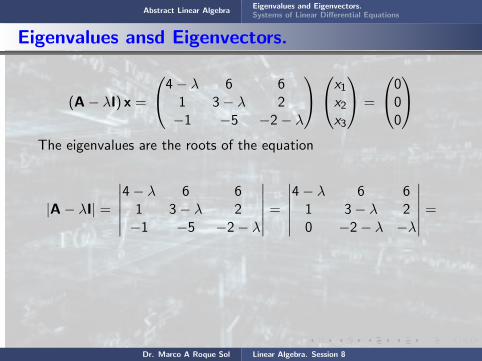
Abstract Linear AlgebraEigenvalues and Eigenvectors.Systems of Linear Differential Equations
Eigenvalues ansd Eigenvectors.
(A− λI) x =
4− λ 6 61 3− λ 2−1 −5 −2− λ
x1x2x3
=
000
The eigenvalues are the roots of the equation
|A− λI| =
∣∣∣∣∣∣4− λ 6 6
1 3− λ 2−1 −5 −2− λ
∣∣∣∣∣∣ =
∣∣∣∣∣∣4− λ 6 6
1 3− λ 20 −2− λ −λ
∣∣∣∣∣∣ =
−
∣∣∣∣∣∣1 3− λ 20 −(4− λ)(3− λ) + 6 6− 2(4− λ)0 −2− λ −λ
∣∣∣∣∣∣ =
− λ3 + 5λ2 − 8λ+ 4 =
−(λ− 1)(λ− 2)2 = 0
Dr. Marco A Roque Sol Linear Algebra. Session 8

Abstract Linear AlgebraEigenvalues and Eigenvectors.Systems of Linear Differential Equations
Eigenvalues ansd Eigenvectors.
(A− λI) x =
4− λ 6 61 3− λ 2−1 −5 −2− λ
x1x2x3
=
000
The eigenvalues are the roots of the equation
|A− λI| =
∣∣∣∣∣∣4− λ 6 6
1 3− λ 2−1 −5 −2− λ
∣∣∣∣∣∣ =
∣∣∣∣∣∣4− λ 6 6
1 3− λ 20 −2− λ −λ
∣∣∣∣∣∣ =
−
∣∣∣∣∣∣1 3− λ 20 −(4− λ)(3− λ) + 6 6− 2(4− λ)0 −2− λ −λ
∣∣∣∣∣∣ = − λ3 + 5λ2 − 8λ+ 4 =
−(λ− 1)(λ− 2)2 = 0
Dr. Marco A Roque Sol Linear Algebra. Session 8
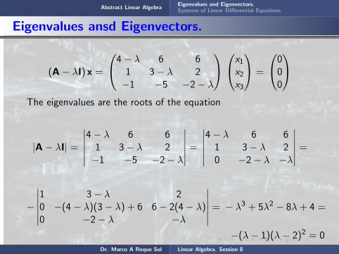
Abstract Linear AlgebraEigenvalues and Eigenvectors.Systems of Linear Differential Equations
Eigenvalues ansd Eigenvectors.
(A− λI) x =
4− λ 6 61 3− λ 2−1 −5 −2− λ
x1x2x3
=
000
The eigenvalues are the roots of the equation
|A− λI| =
∣∣∣∣∣∣4− λ 6 6
1 3− λ 2−1 −5 −2− λ
∣∣∣∣∣∣ =
∣∣∣∣∣∣4− λ 6 6
1 3− λ 20 −2− λ −λ
∣∣∣∣∣∣ =
−
∣∣∣∣∣∣1 3− λ 20 −(4− λ)(3− λ) + 6 6− 2(4− λ)0 −2− λ −λ
∣∣∣∣∣∣ = − λ3 + 5λ2 − 8λ+ 4 =
−(λ− 1)(λ− 2)2 = 0Dr. Marco A Roque Sol Linear Algebra. Session 8

Abstract Linear AlgebraEigenvalues and Eigenvectors.Systems of Linear Differential Equations
Eigenvalues ansd Eigenvectors.
The roots are λ1 = 1, λ2 = 2, and λ3 = 2 .
1) For λ1 = 1
(A− λ1I) x =
4− λ 6 61 3− λ 2−1 −5 −2− λ
x1x2x3
=
3 6 61 2 2−1 −5 −3
x1x2x3
=
000
We can reduce this to the equivalent system
3 6 61 2 20 3 1
=
1 2 21 2 20 3 1
=
1 2 21 −3 −10 0 0
x1x2x3
=
000
Dr. Marco A Roque Sol Linear Algebra. Session 8

Abstract Linear AlgebraEigenvalues and Eigenvectors.Systems of Linear Differential Equations
Eigenvalues ansd Eigenvectors.
The roots
are λ1 = 1, λ2 = 2, and λ3 = 2 .
1) For λ1 = 1
(A− λ1I) x =
4− λ 6 61 3− λ 2−1 −5 −2− λ
x1x2x3
=
3 6 61 2 2−1 −5 −3
x1x2x3
=
000
We can reduce this to the equivalent system
3 6 61 2 20 3 1
=
1 2 21 2 20 3 1
=
1 2 21 −3 −10 0 0
x1x2x3
=
000
Dr. Marco A Roque Sol Linear Algebra. Session 8

Abstract Linear AlgebraEigenvalues and Eigenvectors.Systems of Linear Differential Equations
Eigenvalues ansd Eigenvectors.
The roots are λ1 = 1, λ2 = 2, and λ3 = 2 .
1) For λ1 = 1
(A− λ1I) x =
4− λ 6 61 3− λ 2−1 −5 −2− λ
x1x2x3
=
3 6 61 2 2−1 −5 −3
x1x2x3
=
000
We can reduce this to the equivalent system
3 6 61 2 20 3 1
=
1 2 21 2 20 3 1
=
1 2 21 −3 −10 0 0
x1x2x3
=
000
Dr. Marco A Roque Sol Linear Algebra. Session 8
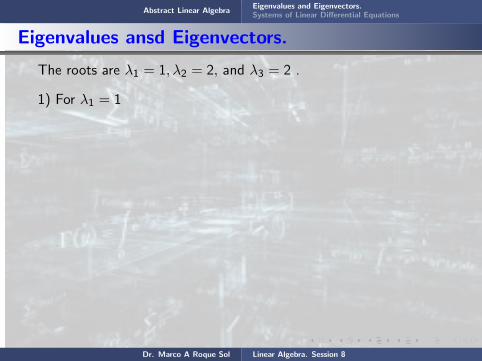
Abstract Linear AlgebraEigenvalues and Eigenvectors.Systems of Linear Differential Equations
Eigenvalues ansd Eigenvectors.
The roots are λ1 = 1, λ2 = 2, and λ3 = 2 .
1) For λ1 = 1
(A− λ1I) x =
4− λ 6 61 3− λ 2−1 −5 −2− λ
x1x2x3
=
3 6 61 2 2−1 −5 −3
x1x2x3
=
000
We can reduce this to the equivalent system
3 6 61 2 20 3 1
=
1 2 21 2 20 3 1
=
1 2 21 −3 −10 0 0
x1x2x3
=
000
Dr. Marco A Roque Sol Linear Algebra. Session 8
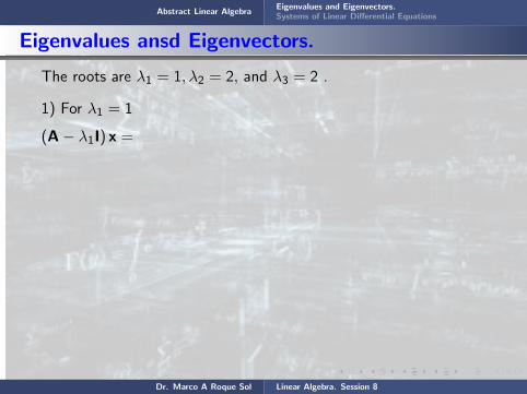
Abstract Linear AlgebraEigenvalues and Eigenvectors.Systems of Linear Differential Equations
Eigenvalues ansd Eigenvectors.
The roots are λ1 = 1, λ2 = 2, and λ3 = 2 .
1) For λ1 = 1
(A− λ1I) x =
4− λ 6 61 3− λ 2−1 −5 −2− λ
x1x2x3
=
3 6 61 2 2−1 −5 −3
x1x2x3
=
000
We can reduce this to the equivalent system
3 6 61 2 20 3 1
=
1 2 21 2 20 3 1
=
1 2 21 −3 −10 0 0
x1x2x3
=
000
Dr. Marco A Roque Sol Linear Algebra. Session 8
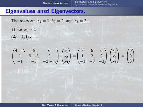
Abstract Linear AlgebraEigenvalues and Eigenvectors.Systems of Linear Differential Equations
Eigenvalues ansd Eigenvectors.
The roots are λ1 = 1, λ2 = 2, and λ3 = 2 .
1) For λ1 = 1
(A− λ1I) x =
4− λ 6 61 3− λ 2−1 −5 −2− λ
x1x2x3
=
3 6 61 2 2−1 −5 −3
x1x2x3
=
000
We can reduce this to the equivalent system
3 6 61 2 20 3 1
=
1 2 21 2 20 3 1
=
1 2 21 −3 −10 0 0
x1x2x3
=
000
Dr. Marco A Roque Sol Linear Algebra. Session 8
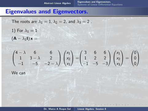
Abstract Linear AlgebraEigenvalues and Eigenvectors.Systems of Linear Differential Equations
Eigenvalues ansd Eigenvectors.
The roots are λ1 = 1, λ2 = 2, and λ3 = 2 .
1) For λ1 = 1
(A− λ1I) x =
4− λ 6 61 3− λ 2−1 −5 −2− λ
x1x2x3
=
3 6 61 2 2−1 −5 −3
x1x2x3
=
000
We can
reduce this to the equivalent system
3 6 61 2 20 3 1
=
1 2 21 2 20 3 1
=
1 2 21 −3 −10 0 0
x1x2x3
=
000
Dr. Marco A Roque Sol Linear Algebra. Session 8
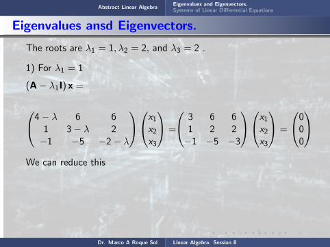
Abstract Linear AlgebraEigenvalues and Eigenvectors.Systems of Linear Differential Equations
Eigenvalues ansd Eigenvectors.
The roots are λ1 = 1, λ2 = 2, and λ3 = 2 .
1) For λ1 = 1
(A− λ1I) x =
4− λ 6 61 3− λ 2−1 −5 −2− λ
x1x2x3
=
3 6 61 2 2−1 −5 −3
x1x2x3
=
000
We can reduce this
to the equivalent system
3 6 61 2 20 3 1
=
1 2 21 2 20 3 1
=
1 2 21 −3 −10 0 0
x1x2x3
=
000
Dr. Marco A Roque Sol Linear Algebra. Session 8

Abstract Linear AlgebraEigenvalues and Eigenvectors.Systems of Linear Differential Equations
Eigenvalues ansd Eigenvectors.
The roots are λ1 = 1, λ2 = 2, and λ3 = 2 .
1) For λ1 = 1
(A− λ1I) x =
4− λ 6 61 3− λ 2−1 −5 −2− λ
x1x2x3
=
3 6 61 2 2−1 −5 −3
x1x2x3
=
000
We can reduce this to the equivalent system
3 6 61 2 20 3 1
=
1 2 21 2 20 3 1
=
1 2 21 −3 −10 0 0
x1x2x3
=
000
Dr. Marco A Roque Sol Linear Algebra. Session 8

Abstract Linear AlgebraEigenvalues and Eigenvectors.Systems of Linear Differential Equations
Eigenvalues ansd Eigenvectors.
The roots are λ1 = 1, λ2 = 2, and λ3 = 2 .
1) For λ1 = 1
(A− λ1I) x =
4− λ 6 61 3− λ 2−1 −5 −2− λ
x1x2x3
=
3 6 61 2 2−1 −5 −3
x1x2x3
=
000
We can reduce this to the equivalent system
3 6 61 2 20 3 1
=
1 2 21 2 20 3 1
=
1 2 21 −3 −10 0 0
x1x2x3
=
000
Dr. Marco A Roque Sol Linear Algebra. Session 8

Abstract Linear AlgebraEigenvalues and Eigenvectors.Systems of Linear Differential Equations
Eigenvalues ansd Eigenvectors.
Solving this system yields the eigenvector
x(1) =
41−3
2) For λ2 = 2
(A− λ2,3I) x =
4− λ 6 61 3− λ 2−1 −5 −2− λ
=
2 6 61 1 2−1 −5 −4
x1x2x3
=
2 6 61 1 2−1 −5 −4
=
1 1 20 4 20 −4 −2
=
1 1 20 4 20 0 0
x1x2x3
=
000
Dr. Marco A Roque Sol Linear Algebra. Session 8
Abstract Linear AlgebraEigenvalues and Eigenvectors.Systems of Linear Differential Equations
Eigenvalues ansd Eigenvectors.
Solving this system
yields the eigenvector
x(1) =
41−3
2) For λ2 = 2
(A− λ2,3I) x =
4− λ 6 61 3− λ 2−1 −5 −2− λ
=
2 6 61 1 2−1 −5 −4
x1x2x3
=
2 6 61 1 2−1 −5 −4
=
1 1 20 4 20 −4 −2
=
1 1 20 4 20 0 0
x1x2x3
=
000
Dr. Marco A Roque Sol Linear Algebra. Session 8

Abstract Linear AlgebraEigenvalues and Eigenvectors.Systems of Linear Differential Equations
Eigenvalues ansd Eigenvectors.
Solving this system yields the eigenvector
x(1) =
41−3
2) For λ2 = 2
(A− λ2,3I) x =
4− λ 6 61 3− λ 2−1 −5 −2− λ
=
2 6 61 1 2−1 −5 −4
x1x2x3
=
2 6 61 1 2−1 −5 −4
=
1 1 20 4 20 −4 −2
=
1 1 20 4 20 0 0
x1x2x3
=
000
Dr. Marco A Roque Sol Linear Algebra. Session 8
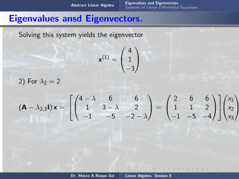
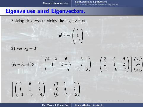
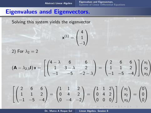

Abstract Linear AlgebraEigenvalues and Eigenvectors.Systems of Linear Differential Equations
Eigenvalues ansd Eigenvectors.
The above system is reduced immediately to the equations
x1 + x2 + 2x3 = 0 4x2 + 2x3 = 0
Two equations and three unknowns. Hence, one of them, is a freevariable, let’s say x3 = α, x2 = 1
2α, and x3 = −2x3 − x2 = −3α .Thus we have
x =
− 3α12α
− 3α
= α
− 312
− 3
Dr. Marco A Roque Sol Linear Algebra. Session 8

Abstract Linear AlgebraEigenvalues and Eigenvectors.Systems of Linear Differential Equations
Eigenvalues ansd Eigenvectors.
The above system
is reduced immediately to the equations
x1 + x2 + 2x3 = 0 4x2 + 2x3 = 0
Two equations and three unknowns. Hence, one of them, is a freevariable, let’s say x3 = α, x2 = 1
2α, and x3 = −2x3 − x2 = −3α .Thus we have
x =
− 3α12α
− 3α
= α
− 312
− 3
Dr. Marco A Roque Sol Linear Algebra. Session 8

Abstract Linear AlgebraEigenvalues and Eigenvectors.Systems of Linear Differential Equations
Eigenvalues ansd Eigenvectors.
The above system is reduced
immediately to the equations
x1 + x2 + 2x3 = 0 4x2 + 2x3 = 0
Two equations and three unknowns. Hence, one of them, is a freevariable, let’s say x3 = α, x2 = 1
2α, and x3 = −2x3 − x2 = −3α .Thus we have
x =
− 3α12α
− 3α
= α
− 312
− 3
Dr. Marco A Roque Sol Linear Algebra. Session 8

Abstract Linear AlgebraEigenvalues and Eigenvectors.Systems of Linear Differential Equations
Eigenvalues ansd Eigenvectors.
The above system is reduced immediately to
the equations
x1 + x2 + 2x3 = 0 4x2 + 2x3 = 0
Two equations and three unknowns. Hence, one of them, is a freevariable, let’s say x3 = α, x2 = 1
2α, and x3 = −2x3 − x2 = −3α .Thus we have
x =
− 3α12α
− 3α
= α
− 312
− 3
Dr. Marco A Roque Sol Linear Algebra. Session 8

Abstract Linear AlgebraEigenvalues and Eigenvectors.Systems of Linear Differential Equations
Eigenvalues ansd Eigenvectors.
The above system is reduced immediately to the equations
x1 + x2 + 2x3 = 0 4x2 + 2x3 = 0
Two equations and three unknowns. Hence, one of them, is a freevariable, let’s say x3 = α, x2 = 1
2α, and x3 = −2x3 − x2 = −3α .Thus we have
x =
− 3α12α
− 3α
= α
− 312
− 3
Dr. Marco A Roque Sol Linear Algebra. Session 8
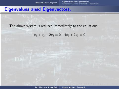
Abstract Linear AlgebraEigenvalues and Eigenvectors.Systems of Linear Differential Equations
Eigenvalues ansd Eigenvectors.
The above system is reduced immediately to the equations
x1 + x2 + 2x3 = 0 4x2 + 2x3 = 0
Two equations and three unknowns. Hence, one of them, is a freevariable, let’s say x3 = α, x2 = 1
2α, and x3 = −2x3 − x2 = −3α .Thus we have
x =
− 3α12α
− 3α
= α
− 312
− 3
Dr. Marco A Roque Sol Linear Algebra. Session 8
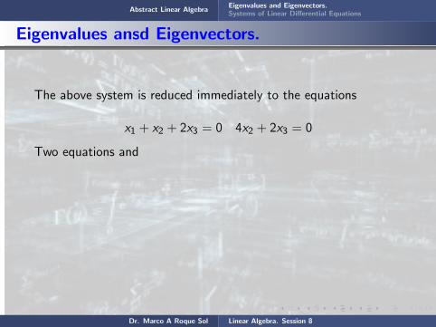
Abstract Linear AlgebraEigenvalues and Eigenvectors.Systems of Linear Differential Equations
Eigenvalues ansd Eigenvectors.
The above system is reduced immediately to the equations
x1 + x2 + 2x3 = 0 4x2 + 2x3 = 0
Two equations and
three unknowns. Hence, one of them, is a freevariable, let’s say x3 = α, x2 = 1
2α, and x3 = −2x3 − x2 = −3α .Thus we have
x =
− 3α12α
− 3α
= α
− 312
− 3
Dr. Marco A Roque Sol Linear Algebra. Session 8

Abstract Linear AlgebraEigenvalues and Eigenvectors.Systems of Linear Differential Equations
Eigenvalues ansd Eigenvectors.
The above system is reduced immediately to the equations
x1 + x2 + 2x3 = 0 4x2 + 2x3 = 0
Two equations and three unknowns.
Hence, one of them, is a freevariable, let’s say x3 = α, x2 = 1
2α, and x3 = −2x3 − x2 = −3α .Thus we have
x =
− 3α12α
− 3α
= α
− 312
− 3
Dr. Marco A Roque Sol Linear Algebra. Session 8
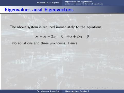
Abstract Linear AlgebraEigenvalues and Eigenvectors.Systems of Linear Differential Equations
Eigenvalues ansd Eigenvectors.
The above system is reduced immediately to the equations
x1 + x2 + 2x3 = 0 4x2 + 2x3 = 0
Two equations and three unknowns. Hence,
one of them, is a freevariable, let’s say x3 = α, x2 = 1
2α, and x3 = −2x3 − x2 = −3α .Thus we have
x =
− 3α12α
− 3α
= α
− 312
− 3
Dr. Marco A Roque Sol Linear Algebra. Session 8

Abstract Linear AlgebraEigenvalues and Eigenvectors.Systems of Linear Differential Equations
Eigenvalues ansd Eigenvectors.
The above system is reduced immediately to the equations
x1 + x2 + 2x3 = 0 4x2 + 2x3 = 0
Two equations and three unknowns. Hence, one of them,
is a freevariable, let’s say x3 = α, x2 = 1
2α, and x3 = −2x3 − x2 = −3α .Thus we have
x =
− 3α12α
− 3α
= α
− 312
− 3
Dr. Marco A Roque Sol Linear Algebra. Session 8

Abstract Linear AlgebraEigenvalues and Eigenvectors.Systems of Linear Differential Equations
Eigenvalues ansd Eigenvectors.
The above system is reduced immediately to the equations
x1 + x2 + 2x3 = 0 4x2 + 2x3 = 0
Two equations and three unknowns. Hence, one of them, is a freevariable,
let’s say x3 = α, x2 = 12α, and x3 = −2x3 − x2 = −3α .
Thus we have
x =
− 3α12α
− 3α
= α
− 312
− 3
Dr. Marco A Roque Sol Linear Algebra. Session 8

Abstract Linear AlgebraEigenvalues and Eigenvectors.Systems of Linear Differential Equations
Eigenvalues ansd Eigenvectors.
The above system is reduced immediately to the equations
x1 + x2 + 2x3 = 0 4x2 + 2x3 = 0
Two equations and three unknowns. Hence, one of them, is a freevariable, let’s say x3 = α,
x2 = 12α, and x3 = −2x3 − x2 = −3α .
Thus we have
x =
− 3α12α
− 3α
= α
− 312
− 3
Dr. Marco A Roque Sol Linear Algebra. Session 8
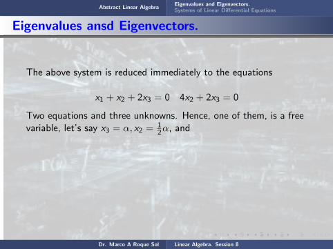
Abstract Linear AlgebraEigenvalues and Eigenvectors.Systems of Linear Differential Equations
Eigenvalues ansd Eigenvectors.
The above system is reduced immediately to the equations
x1 + x2 + 2x3 = 0 4x2 + 2x3 = 0
Two equations and three unknowns. Hence, one of them, is a freevariable, let’s say x3 = α, x2 = 1
2α, and
x3 = −2x3 − x2 = −3α .Thus we have
x =
− 3α12α
− 3α
= α
− 312
− 3
Dr. Marco A Roque Sol Linear Algebra. Session 8

Abstract Linear AlgebraEigenvalues and Eigenvectors.Systems of Linear Differential Equations
Eigenvalues ansd Eigenvectors.
The above system is reduced immediately to the equations
x1 + x2 + 2x3 = 0 4x2 + 2x3 = 0
Two equations and three unknowns. Hence, one of them, is a freevariable, let’s say x3 = α, x2 = 1
2α, and x3 = −2x3 − x2 = −3α .
Thus we have
x =
− 3α12α
− 3α
= α
− 312
− 3
Dr. Marco A Roque Sol Linear Algebra. Session 8

Abstract Linear AlgebraEigenvalues and Eigenvectors.Systems of Linear Differential Equations
Eigenvalues ansd Eigenvectors.
The above system is reduced immediately to the equations
x1 + x2 + 2x3 = 0 4x2 + 2x3 = 0
Two equations and three unknowns. Hence, one of them, is a freevariable, let’s say x3 = α, x2 = 1
2α, and x3 = −2x3 − x2 = −3α .Thus we have
x =
− 3α12α
− 3α
= α
− 312
− 3
Dr. Marco A Roque Sol Linear Algebra. Session 8
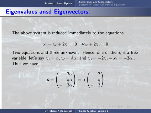
Abstract Linear AlgebraEigenvalues and Eigenvectors.Systems of Linear Differential Equations
Eigenvalues ansd Eigenvectors.
The above system is reduced immediately to the equations
x1 + x2 + 2x3 = 0 4x2 + 2x3 = 0
Two equations and three unknowns. Hence, one of them, is a freevariable, let’s say x3 = α, x2 = 1
2α, and x3 = −2x3 − x2 = −3α .Thus we have
x =
− 3α12α
− 3α
= α
− 312
− 3
Dr. Marco A Roque Sol Linear Algebra. Session 8

Abstract Linear AlgebraEigenvalues and Eigenvectors.Systems of Linear Differential Equations
Eigenvalues ansd Eigenvectors.
In this way, there is one linearly independent eigenvector associatedtoλ2,3 = 2 , namely,
x(2) =
31
− 2
Therefore, there are just two linearly independent eigenvectors
x(1) =
111
x(2) =
41
− 3
that is, the matrix A is defective
Dr. Marco A Roque Sol Linear Algebra. Session 8
Abstract Linear AlgebraEigenvalues and Eigenvectors.Systems of Linear Differential Equations
Eigenvalues ansd Eigenvectors.
In this way,
there is one linearly independent eigenvector associatedtoλ2,3 = 2 , namely,
x(2) =
31
− 2
Therefore, there are just two linearly independent eigenvectors
x(1) =
111
x(2) =
41
− 3
that is, the matrix A is defective
Dr. Marco A Roque Sol Linear Algebra. Session 8

Abstract Linear AlgebraEigenvalues and Eigenvectors.Systems of Linear Differential Equations
Eigenvalues ansd Eigenvectors.
In this way, there is one
linearly independent eigenvector associatedtoλ2,3 = 2 , namely,
x(2) =
31
− 2
Therefore, there are just two linearly independent eigenvectors
x(1) =
111
x(2) =
41
− 3
that is, the matrix A is defective
Dr. Marco A Roque Sol Linear Algebra. Session 8
Abstract Linear AlgebraEigenvalues and Eigenvectors.Systems of Linear Differential Equations
Eigenvalues ansd Eigenvectors.
In this way, there is one linearly independent
eigenvector associatedtoλ2,3 = 2 , namely,
x(2) =
31
− 2
Therefore, there are just two linearly independent eigenvectors
x(1) =
111
x(2) =
41
− 3
that is, the matrix A is defective
Dr. Marco A Roque Sol Linear Algebra. Session 8

Abstract Linear AlgebraEigenvalues and Eigenvectors.Systems of Linear Differential Equations
Eigenvalues ansd Eigenvectors.
In this way, there is one linearly independent eigenvector
associatedtoλ2,3 = 2 , namely,
x(2) =
31
− 2
Therefore, there are just two linearly independent eigenvectors
x(1) =
111
x(2) =
41
− 3
that is, the matrix A is defective
Dr. Marco A Roque Sol Linear Algebra. Session 8

Abstract Linear AlgebraEigenvalues and Eigenvectors.Systems of Linear Differential Equations
Eigenvalues ansd Eigenvectors.
In this way, there is one linearly independent eigenvector associatedto
λ2,3 = 2 , namely,
x(2) =
31
− 2
Therefore, there are just two linearly independent eigenvectors
x(1) =
111
x(2) =
41
− 3
that is, the matrix A is defective
Dr. Marco A Roque Sol Linear Algebra. Session 8
Abstract Linear AlgebraEigenvalues and Eigenvectors.Systems of Linear Differential Equations
Eigenvalues ansd Eigenvectors.
In this way, there is one linearly independent eigenvector associatedtoλ2,3 = 2 , namely,
x(2) =
31
− 2
Therefore, there are just two linearly independent eigenvectors
x(1) =
111
x(2) =
41
− 3
that is, the matrix A is defective
Dr. Marco A Roque Sol Linear Algebra. Session 8

Abstract Linear AlgebraEigenvalues and Eigenvectors.Systems of Linear Differential Equations
Eigenvalues ansd Eigenvectors.
In this way, there is one linearly independent eigenvector associatedtoλ2,3 = 2 , namely,
x(2) =
31
− 2
Therefore,
there are just two linearly independent eigenvectors
x(1) =
111
x(2) =
41
− 3
that is, the matrix A is defective
Dr. Marco A Roque Sol Linear Algebra. Session 8

Abstract Linear AlgebraEigenvalues and Eigenvectors.Systems of Linear Differential Equations
Eigenvalues ansd Eigenvectors.
In this way, there is one linearly independent eigenvector associatedtoλ2,3 = 2 , namely,
x(2) =
31
− 2
Therefore, there are
just two linearly independent eigenvectors
x(1) =
111
x(2) =
41
− 3
that is, the matrix A is defective
Dr. Marco A Roque Sol Linear Algebra. Session 8

Abstract Linear AlgebraEigenvalues and Eigenvectors.Systems of Linear Differential Equations
Eigenvalues ansd Eigenvectors.
In this way, there is one linearly independent eigenvector associatedtoλ2,3 = 2 , namely,
x(2) =
31
− 2
Therefore, there are just two linearly
independent eigenvectors
x(1) =
111
x(2) =
41
− 3
that is, the matrix A is defective
Dr. Marco A Roque Sol Linear Algebra. Session 8
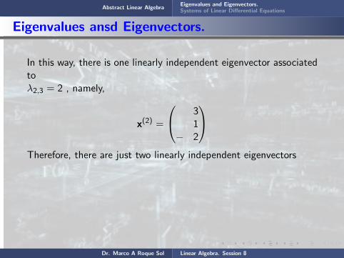
Abstract Linear AlgebraEigenvalues and Eigenvectors.Systems of Linear Differential Equations
Eigenvalues ansd Eigenvectors.
In this way, there is one linearly independent eigenvector associatedtoλ2,3 = 2 , namely,
x(2) =
31
− 2
Therefore, there are just two linearly independent eigenvectors
x(1) =
111
x(2) =
41
− 3
that is, the matrix A is defective
Dr. Marco A Roque Sol Linear Algebra. Session 8

Abstract Linear AlgebraEigenvalues and Eigenvectors.Systems of Linear Differential Equations
Eigenvalues ansd Eigenvectors.
In this way, there is one linearly independent eigenvector associatedtoλ2,3 = 2 , namely,
x(2) =
31
− 2
Therefore, there are just two linearly independent eigenvectors
x(1) =
111
x(2) =
41
− 3
that is,
the matrix A is defective
Dr. Marco A Roque Sol Linear Algebra. Session 8
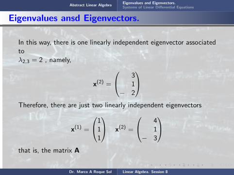
Abstract Linear AlgebraEigenvalues and Eigenvectors.Systems of Linear Differential Equations
Eigenvalues ansd Eigenvectors.
In this way, there is one linearly independent eigenvector associatedtoλ2,3 = 2 , namely,
x(2) =
31
− 2
Therefore, there are just two linearly independent eigenvectors
x(1) =
111
x(2) =
41
− 3
that is, the matrix A
is defective
Dr. Marco A Roque Sol Linear Algebra. Session 8

Abstract Linear AlgebraEigenvalues and Eigenvectors.Systems of Linear Differential Equations
Eigenvalues ansd Eigenvectors.
In this way, there is one linearly independent eigenvector associatedtoλ2,3 = 2 , namely,
x(2) =
31
− 2
Therefore, there are just two linearly independent eigenvectors
x(1) =
111
x(2) =
41
− 3
that is, the matrix A is defective
Dr. Marco A Roque Sol Linear Algebra. Session 8

Abstract Linear AlgebraEigenvalues and Eigenvectors.Systems of Linear Differential Equations
Eigenvalues ansd Eigenvectors.
Example 9.4
Find the eigenvalues and eigenvectors of the matrix
A =
1 0 02 1 −23 2 1
Solution
The eigenvalues λ andeigenvectors x satisfy the equation(A− λI) x = 0, or
Dr. Marco A Roque Sol Linear Algebra. Session 8

Abstract Linear AlgebraEigenvalues and Eigenvectors.Systems of Linear Differential Equations
Eigenvalues ansd Eigenvectors.
Example 9.4
Find the eigenvalues and
eigenvectors of the matrix
A =
1 0 02 1 −23 2 1
Solution
The eigenvalues λ andeigenvectors x satisfy the equation(A− λI) x = 0, or
Dr. Marco A Roque Sol Linear Algebra. Session 8

Abstract Linear AlgebraEigenvalues and Eigenvectors.Systems of Linear Differential Equations
Eigenvalues ansd Eigenvectors.
Example 9.4
Find the eigenvalues and eigenvectors of the matrix
A =
1 0 02 1 −23 2 1
Solution
The eigenvalues λ andeigenvectors x satisfy the equation(A− λI) x = 0, or
Dr. Marco A Roque Sol Linear Algebra. Session 8

Abstract Linear AlgebraEigenvalues and Eigenvectors.Systems of Linear Differential Equations
Eigenvalues ansd Eigenvectors.
Example 9.4
Find the eigenvalues and eigenvectors of the matrix
A =
1 0 02 1 −23 2 1
Solution
The eigenvalues
λ andeigenvectors x satisfy the equation(A− λI) x = 0, or
Dr. Marco A Roque Sol Linear Algebra. Session 8

Abstract Linear AlgebraEigenvalues and Eigenvectors.Systems of Linear Differential Equations
Eigenvalues ansd Eigenvectors.
Example 9.4
Find the eigenvalues and eigenvectors of the matrix
A =
1 0 02 1 −23 2 1
Solution
The eigenvalues λ and
eigenvectors x satisfy the equation(A− λI) x = 0, or
Dr. Marco A Roque Sol Linear Algebra. Session 8
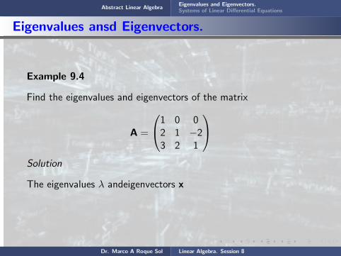
Abstract Linear AlgebraEigenvalues and Eigenvectors.Systems of Linear Differential Equations
Eigenvalues ansd Eigenvectors.
Example 9.4
Find the eigenvalues and eigenvectors of the matrix
A =
1 0 02 1 −23 2 1
Solution
The eigenvalues λ andeigenvectors x
satisfy the equation(A− λI) x = 0, or
Dr. Marco A Roque Sol Linear Algebra. Session 8

Abstract Linear AlgebraEigenvalues and Eigenvectors.Systems of Linear Differential Equations
Eigenvalues ansd Eigenvectors.
Example 9.4
Find the eigenvalues and eigenvectors of the matrix
A =
1 0 02 1 −23 2 1
Solution
The eigenvalues λ andeigenvectors x satisfy the equation
(A− λI) x = 0, or
Dr. Marco A Roque Sol Linear Algebra. Session 8
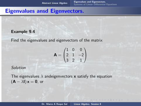
Abstract Linear AlgebraEigenvalues and Eigenvectors.Systems of Linear Differential Equations
Eigenvalues ansd Eigenvectors.
Example 9.4
Find the eigenvalues and eigenvectors of the matrix
A =
1 0 02 1 −23 2 1
Solution
The eigenvalues λ andeigenvectors x satisfy the equation(A− λI) x = 0, or
Dr. Marco A Roque Sol Linear Algebra. Session 8

Abstract Linear AlgebraEigenvalues and Eigenvectors.Systems of Linear Differential Equations
Eigenvalues ansd Eigenvectors.
(A− λI) x =
1− λ 0 02 1− λ −23 2 1− λ
x1x2x3
=
000
The eigenvalues are the roots of the equation
|A− λI| =
∣∣∣∣∣∣1− λ 0 0
2 1− λ −23 2 1− λ
∣∣∣∣∣∣ = (1− λ)
∣∣∣∣1− λ −22 1− λ
∣∣∣∣ =
(1− λ)3 + 4(1− λ) = (1− λ)(λ2 − 2λ+ 5) = 0
Dr. Marco A Roque Sol Linear Algebra. Session 8

Abstract Linear AlgebraEigenvalues and Eigenvectors.Systems of Linear Differential Equations
Eigenvalues ansd Eigenvectors.
(A− λI) x =
1− λ 0 02 1− λ −23 2 1− λ
x1x2x3
=
000
The eigenvalues
are the roots of the equation
|A− λI| =
∣∣∣∣∣∣1− λ 0 0
2 1− λ −23 2 1− λ
∣∣∣∣∣∣ = (1− λ)
∣∣∣∣1− λ −22 1− λ
∣∣∣∣ =
(1− λ)3 + 4(1− λ) = (1− λ)(λ2 − 2λ+ 5) = 0
Dr. Marco A Roque Sol Linear Algebra. Session 8
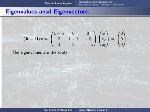
Abstract Linear AlgebraEigenvalues and Eigenvectors.Systems of Linear Differential Equations
Eigenvalues ansd Eigenvectors.
(A− λI) x =
1− λ 0 02 1− λ −23 2 1− λ
x1x2x3
=
000
The eigenvalues are the roots
of the equation
|A− λI| =
∣∣∣∣∣∣1− λ 0 0
2 1− λ −23 2 1− λ
∣∣∣∣∣∣ = (1− λ)
∣∣∣∣1− λ −22 1− λ
∣∣∣∣ =
(1− λ)3 + 4(1− λ) = (1− λ)(λ2 − 2λ+ 5) = 0
Dr. Marco A Roque Sol Linear Algebra. Session 8
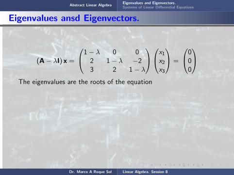
Abstract Linear AlgebraEigenvalues and Eigenvectors.Systems of Linear Differential Equations
Eigenvalues ansd Eigenvectors.
(A− λI) x =
1− λ 0 02 1− λ −23 2 1− λ
x1x2x3
=
000
The eigenvalues are the roots of the equation
|A− λI| =
∣∣∣∣∣∣1− λ 0 0
2 1− λ −23 2 1− λ
∣∣∣∣∣∣ = (1− λ)
∣∣∣∣1− λ −22 1− λ
∣∣∣∣ =
(1− λ)3 + 4(1− λ) = (1− λ)(λ2 − 2λ+ 5) = 0
Dr. Marco A Roque Sol Linear Algebra. Session 8

Abstract Linear AlgebraEigenvalues and Eigenvectors.Systems of Linear Differential Equations
Eigenvalues ansd Eigenvectors.
(A− λI) x =
1− λ 0 02 1− λ −23 2 1− λ
x1x2x3
=
000
The eigenvalues are the roots of the equation
|A− λI| =
∣∣∣∣∣∣1− λ 0 0
2 1− λ −23 2 1− λ
∣∣∣∣∣∣ =
(1− λ)
∣∣∣∣1− λ −22 1− λ
∣∣∣∣ =
(1− λ)3 + 4(1− λ) = (1− λ)(λ2 − 2λ+ 5) = 0
Dr. Marco A Roque Sol Linear Algebra. Session 8

Abstract Linear AlgebraEigenvalues and Eigenvectors.Systems of Linear Differential Equations
Eigenvalues ansd Eigenvectors.
(A− λI) x =
1− λ 0 02 1− λ −23 2 1− λ
x1x2x3
=
000
The eigenvalues are the roots of the equation
|A− λI| =
∣∣∣∣∣∣1− λ 0 0
2 1− λ −23 2 1− λ
∣∣∣∣∣∣ = (1− λ)
∣∣∣∣1− λ −22 1− λ
∣∣∣∣ =
(1− λ)3 + 4(1− λ) = (1− λ)(λ2 − 2λ+ 5) = 0
Dr. Marco A Roque Sol Linear Algebra. Session 8

Abstract Linear AlgebraEigenvalues and Eigenvectors.Systems of Linear Differential Equations
Eigenvalues ansd Eigenvectors.
(A− λI) x =
1− λ 0 02 1− λ −23 2 1− λ
x1x2x3
=
000
The eigenvalues are the roots of the equation
|A− λI| =
∣∣∣∣∣∣1− λ 0 0
2 1− λ −23 2 1− λ
∣∣∣∣∣∣ = (1− λ)
∣∣∣∣1− λ −22 1− λ
∣∣∣∣ =
(1− λ)3 + 4(1− λ) = (1− λ)(λ2 − 2λ+ 5) = 0
Dr. Marco A Roque Sol Linear Algebra. Session 8
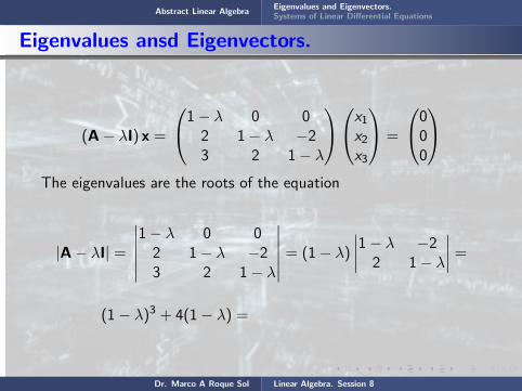
Abstract Linear AlgebraEigenvalues and Eigenvectors.Systems of Linear Differential Equations
Eigenvalues ansd Eigenvectors.
(A− λI) x =
1− λ 0 02 1− λ −23 2 1− λ
x1x2x3
=
000
The eigenvalues are the roots of the equation
|A− λI| =
∣∣∣∣∣∣1− λ 0 0
2 1− λ −23 2 1− λ
∣∣∣∣∣∣ = (1− λ)
∣∣∣∣1− λ −22 1− λ
∣∣∣∣ =
(1− λ)3 + 4(1− λ) =
(1− λ)(λ2 − 2λ+ 5) = 0
Dr. Marco A Roque Sol Linear Algebra. Session 8
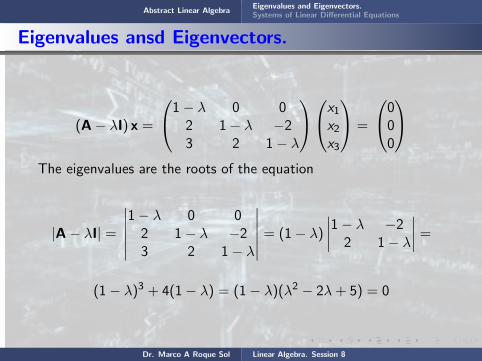
Abstract Linear AlgebraEigenvalues and Eigenvectors.Systems of Linear Differential Equations
Eigenvalues ansd Eigenvectors.
(A− λI) x =
1− λ 0 02 1− λ −23 2 1− λ
x1x2x3
=
000
The eigenvalues are the roots of the equation
|A− λI| =
∣∣∣∣∣∣1− λ 0 0
2 1− λ −23 2 1− λ
∣∣∣∣∣∣ = (1− λ)
∣∣∣∣1− λ −22 1− λ
∣∣∣∣ =
(1− λ)3 + 4(1− λ) = (1− λ)(λ2 − 2λ+ 5) = 0
Dr. Marco A Roque Sol Linear Algebra. Session 8

Abstract Linear AlgebraEigenvalues and Eigenvectors.Systems of Linear Differential Equations
Eigenvalues ansd Eigenvectors.
The roots are λ1 = 1, λ2 = 1 + 2 i , and λ3 = 1− 2 i .
1) For λ1 = 1
(A− λ1I) x =
1− λ 0 02 1− λ −23 2 1− λ
=
0 0 02 0 −23 2 0
x1x2x3
=
000
We can reduce this to the equivalent system
2 0 −20 0 03 2 0
=
1 0 −10 0 03 2 0
=
1 0 −10 2 40 0 0
x1x2x3
=
000
Dr. Marco A Roque Sol Linear Algebra. Session 8
Abstract Linear AlgebraEigenvalues and Eigenvectors.Systems of Linear Differential Equations
Eigenvalues ansd Eigenvectors.
The roots
are λ1 = 1, λ2 = 1 + 2 i , and λ3 = 1− 2 i .
1) For λ1 = 1
(A− λ1I) x =
1− λ 0 02 1− λ −23 2 1− λ
=
0 0 02 0 −23 2 0
x1x2x3
=
000
We can reduce this to the equivalent system
2 0 −20 0 03 2 0
=
1 0 −10 0 03 2 0
=
1 0 −10 2 40 0 0
x1x2x3
=
000
Dr. Marco A Roque Sol Linear Algebra. Session 8
Abstract Linear AlgebraEigenvalues and Eigenvectors.Systems of Linear Differential Equations
Eigenvalues ansd Eigenvectors.
The roots are λ1 = 1, λ2 = 1 + 2 i , and λ3 = 1− 2 i .
1) For λ1 = 1
(A− λ1I) x =
1− λ 0 02 1− λ −23 2 1− λ
=
0 0 02 0 −23 2 0
x1x2x3
=
000
We can reduce this to the equivalent system
2 0 −20 0 03 2 0
=
1 0 −10 0 03 2 0
=
1 0 −10 2 40 0 0
x1x2x3
=
000
Dr. Marco A Roque Sol Linear Algebra. Session 8
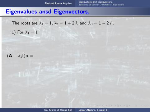
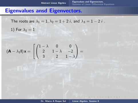
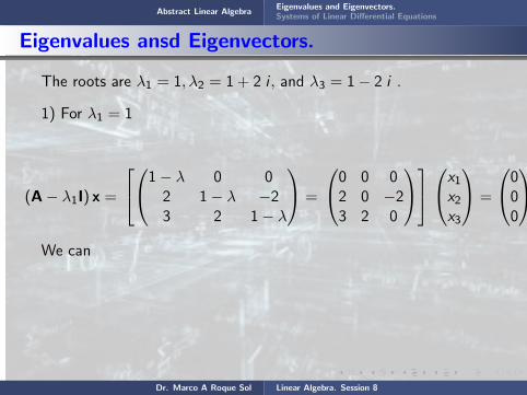
Abstract Linear AlgebraEigenvalues and Eigenvectors.Systems of Linear Differential Equations
Eigenvalues ansd Eigenvectors.
The roots are λ1 = 1, λ2 = 1 + 2 i , and λ3 = 1− 2 i .
1) For λ1 = 1
(A− λ1I) x =
1− λ 0 02 1− λ −23 2 1− λ
=
0 0 02 0 −23 2 0
x1x2x3
=
000
We can
reduce this to the equivalent system
2 0 −20 0 03 2 0
=
1 0 −10 0 03 2 0
=
1 0 −10 2 40 0 0
x1x2x3
=
000
Dr. Marco A Roque Sol Linear Algebra. Session 8
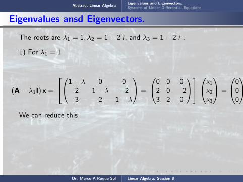
Abstract Linear AlgebraEigenvalues and Eigenvectors.Systems of Linear Differential Equations
Eigenvalues ansd Eigenvectors.
The roots are λ1 = 1, λ2 = 1 + 2 i , and λ3 = 1− 2 i .
1) For λ1 = 1
(A− λ1I) x =
1− λ 0 02 1− λ −23 2 1− λ
=
0 0 02 0 −23 2 0
x1x2x3
=
000
We can reduce this
to the equivalent system
2 0 −20 0 03 2 0
=
1 0 −10 0 03 2 0
=
1 0 −10 2 40 0 0
x1x2x3
=
000
Dr. Marco A Roque Sol Linear Algebra. Session 8

Abstract Linear AlgebraEigenvalues and Eigenvectors.Systems of Linear Differential Equations
Eigenvalues ansd Eigenvectors.
The roots are λ1 = 1, λ2 = 1 + 2 i , and λ3 = 1− 2 i .
1) For λ1 = 1
(A− λ1I) x =
1− λ 0 02 1− λ −23 2 1− λ
=
0 0 02 0 −23 2 0
x1x2x3
=
000
We can reduce this to the equivalent system
2 0 −20 0 03 2 0
=
1 0 −10 0 03 2 0
=
1 0 −10 2 40 0 0
x1x2x3
=
000
Dr. Marco A Roque Sol Linear Algebra. Session 8

Abstract Linear AlgebraEigenvalues and Eigenvectors.Systems of Linear Differential Equations
Eigenvalues ansd Eigenvectors.
The roots are λ1 = 1, λ2 = 1 + 2 i , and λ3 = 1− 2 i .
1) For λ1 = 1
(A− λ1I) x =
1− λ 0 02 1− λ −23 2 1− λ
=
0 0 02 0 −23 2 0
x1x2x3
=
000
We can reduce this to the equivalent system
2 0 −20 0 03 2 0
=
1 0 −10 0 03 2 0
=
1 0 −10 2 40 0 0
x1x2x3
=
000
Dr. Marco A Roque Sol Linear Algebra. Session 8
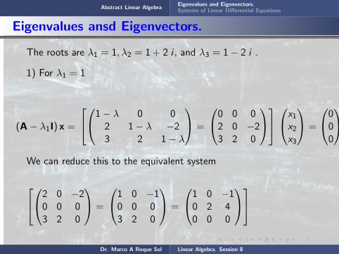
Abstract Linear AlgebraEigenvalues and Eigenvectors.Systems of Linear Differential Equations
Eigenvalues ansd Eigenvectors.
The roots are λ1 = 1, λ2 = 1 + 2 i , and λ3 = 1− 2 i .
1) For λ1 = 1
(A− λ1I) x =
1− λ 0 02 1− λ −23 2 1− λ
=
0 0 02 0 −23 2 0
x1x2x3
=
000
We can reduce this to the equivalent system
2 0 −20 0 03 2 0
=
1 0 −10 0 03 2 0
=
1 0 −10 2 40 0 0
x1x2x3
=
000
Dr. Marco A Roque Sol Linear Algebra. Session 8

Abstract Linear AlgebraEigenvalues and Eigenvectors.Systems of Linear Differential Equations
Eigenvalues ansd Eigenvectors.
Solving this system yields the eigenvector
x(1) =
1− 3/2
1
2) For λ2 = 1 + 2 i
(A− λ2I) x =
1− λ 0 02 1− λ −23 2 1− λ
x1x2x3
=
−2 i 0 02 −2 i −23 2 −2 i
x1x2x3
=
000
Dr. Marco A Roque Sol Linear Algebra. Session 8
Abstract Linear AlgebraEigenvalues and Eigenvectors.Systems of Linear Differential Equations
Eigenvalues ansd Eigenvectors.
Solving this system
yields the eigenvector
x(1) =
1− 3/2
1
2) For λ2 = 1 + 2 i
(A− λ2I) x =
1− λ 0 02 1− λ −23 2 1− λ
x1x2x3
=
−2 i 0 02 −2 i −23 2 −2 i
x1x2x3
=
000
Dr. Marco A Roque Sol Linear Algebra. Session 8
Abstract Linear AlgebraEigenvalues and Eigenvectors.Systems of Linear Differential Equations
Eigenvalues ansd Eigenvectors.
Solving this system yields the eigenvector
x(1) =
1− 3/2
1
2) For λ2 = 1 + 2 i
(A− λ2I) x =
1− λ 0 02 1− λ −23 2 1− λ
x1x2x3
=
−2 i 0 02 −2 i −23 2 −2 i
x1x2x3
=
000
Dr. Marco A Roque Sol Linear Algebra. Session 8
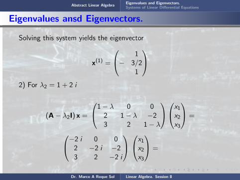

Abstract Linear AlgebraEigenvalues and Eigenvectors.Systems of Linear Differential Equations
Eigenvalues ansd Eigenvectors.
The above system is reduced immediately to the equations
x1 = 0 − 2 ix2 − 2x3 = 0, 2x2 − 2 ix3 = 0
Thus, we have one equation and two unknowns. Hence, one ofthem 1 is a free veriable, let’s say x2 = α, x3 = −i α . Hence
x =
0α−i α
= α
01
− i
= α
010
− i
001
Dr. Marco A Roque Sol Linear Algebra. Session 8

Abstract Linear AlgebraEigenvalues and Eigenvectors.Systems of Linear Differential Equations
Eigenvalues ansd Eigenvectors.
The above system
is reduced immediately to the equations
x1 = 0 − 2 ix2 − 2x3 = 0, 2x2 − 2 ix3 = 0
Thus, we have one equation and two unknowns. Hence, one ofthem 1 is a free veriable, let’s say x2 = α, x3 = −i α . Hence
x =
0α−i α
= α
01
− i
= α
010
− i
001
Dr. Marco A Roque Sol Linear Algebra. Session 8
Abstract Linear AlgebraEigenvalues and Eigenvectors.Systems of Linear Differential Equations
Eigenvalues ansd Eigenvectors.
The above system is reduced immediately
to the equations
x1 = 0 − 2 ix2 − 2x3 = 0, 2x2 − 2 ix3 = 0
Thus, we have one equation and two unknowns. Hence, one ofthem 1 is a free veriable, let’s say x2 = α, x3 = −i α . Hence
x =
0α−i α
= α
01
− i
= α
010
− i
001
Dr. Marco A Roque Sol Linear Algebra. Session 8

Abstract Linear AlgebraEigenvalues and Eigenvectors.Systems of Linear Differential Equations
Eigenvalues ansd Eigenvectors.
The above system is reduced immediately to the equations
x1 = 0 − 2 ix2 − 2x3 = 0, 2x2 − 2 ix3 = 0
Thus, we have one equation and two unknowns. Hence, one ofthem 1 is a free veriable, let’s say x2 = α, x3 = −i α . Hence
x =
0α−i α
= α
01
− i
= α
010
− i
001
Dr. Marco A Roque Sol Linear Algebra. Session 8

Abstract Linear AlgebraEigenvalues and Eigenvectors.Systems of Linear Differential Equations
Eigenvalues ansd Eigenvectors.
The above system is reduced immediately to the equations
x1 = 0 − 2 ix2 − 2x3 = 0, 2x2 − 2 ix3 = 0
Thus, we have one equation and two unknowns. Hence, one ofthem 1 is a free veriable, let’s say x2 = α, x3 = −i α . Hence
x =
0α−i α
= α
01
− i
= α
010
− i
001
Dr. Marco A Roque Sol Linear Algebra. Session 8
Abstract Linear AlgebraEigenvalues and Eigenvectors.Systems of Linear Differential Equations
Eigenvalues ansd Eigenvectors.
The above system is reduced immediately to the equations
x1 = 0 − 2 ix2 − 2x3 = 0, 2x2 − 2 ix3 = 0
Thus, we have
one equation and two unknowns. Hence, one ofthem 1 is a free veriable, let’s say x2 = α, x3 = −i α . Hence
x =
0α−i α
= α
01
− i
= α
010
− i
001
Dr. Marco A Roque Sol Linear Algebra. Session 8
Abstract Linear AlgebraEigenvalues and Eigenvectors.Systems of Linear Differential Equations
Eigenvalues ansd Eigenvectors.
The above system is reduced immediately to the equations
x1 = 0 − 2 ix2 − 2x3 = 0, 2x2 − 2 ix3 = 0
Thus, we have one equation and two unknowns. Hence,
one ofthem 1 is a free veriable, let’s say x2 = α, x3 = −i α . Hence
x =
0α−i α
= α
01
− i
= α
010
− i
001
Dr. Marco A Roque Sol Linear Algebra. Session 8

Abstract Linear AlgebraEigenvalues and Eigenvectors.Systems of Linear Differential Equations
Eigenvalues ansd Eigenvectors.
The above system is reduced immediately to the equations
x1 = 0 − 2 ix2 − 2x3 = 0, 2x2 − 2 ix3 = 0
Thus, we have one equation and two unknowns. Hence, one ofthem 1 is a free veriable,
let’s say x2 = α, x3 = −i α . Hence
x =
0α−i α
= α
01
− i
= α
010
− i
001
Dr. Marco A Roque Sol Linear Algebra. Session 8

Abstract Linear AlgebraEigenvalues and Eigenvectors.Systems of Linear Differential Equations
Eigenvalues ansd Eigenvectors.
The above system is reduced immediately to the equations
x1 = 0 − 2 ix2 − 2x3 = 0, 2x2 − 2 ix3 = 0
Thus, we have one equation and two unknowns. Hence, one ofthem 1 is a free veriable, let’s say x2 = α,
x3 = −i α . Hence
x =
0α−i α
= α
01
− i
= α
010
− i
001
Dr. Marco A Roque Sol Linear Algebra. Session 8

Abstract Linear AlgebraEigenvalues and Eigenvectors.Systems of Linear Differential Equations
Eigenvalues ansd Eigenvectors.
The above system is reduced immediately to the equations
x1 = 0 − 2 ix2 − 2x3 = 0, 2x2 − 2 ix3 = 0
Thus, we have one equation and two unknowns. Hence, one ofthem 1 is a free veriable, let’s say x2 = α, x3 = −i α .
Hence
x =
0α−i α
= α
01
− i
= α
010
− i
001
Dr. Marco A Roque Sol Linear Algebra. Session 8

Abstract Linear AlgebraEigenvalues and Eigenvectors.Systems of Linear Differential Equations
Eigenvalues ansd Eigenvectors.
The above system is reduced immediately to the equations
x1 = 0 − 2 ix2 − 2x3 = 0, 2x2 − 2 ix3 = 0
Thus, we have one equation and two unknowns. Hence, one ofthem 1 is a free veriable, let’s say x2 = α, x3 = −i α . Hence
x =
0α−i α
= α
01
− i
= α
010
− i
001
Dr. Marco A Roque Sol Linear Algebra. Session 8

Abstract Linear AlgebraEigenvalues and Eigenvectors.Systems of Linear Differential Equations
Eigenvalues ansd Eigenvectors.
The above system is reduced immediately to the equations
x1 = 0 − 2 ix2 − 2x3 = 0, 2x2 − 2 ix3 = 0
Thus, we have one equation and two unknowns. Hence, one ofthem 1 is a free veriable, let’s say x2 = α, x3 = −i α . Hence
x =
0α−i α
=
α
01
− i
= α
010
− i
001
Dr. Marco A Roque Sol Linear Algebra. Session 8

Abstract Linear AlgebraEigenvalues and Eigenvectors.Systems of Linear Differential Equations
Eigenvalues ansd Eigenvectors.
The above system is reduced immediately to the equations
x1 = 0 − 2 ix2 − 2x3 = 0, 2x2 − 2 ix3 = 0
Thus, we have one equation and two unknowns. Hence, one ofthem 1 is a free veriable, let’s say x2 = α, x3 = −i α . Hence
x =
0α−i α
= α
01
− i
=
α
010
− i
001
Dr. Marco A Roque Sol Linear Algebra. Session 8
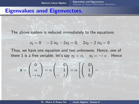
Abstract Linear AlgebraEigenvalues and Eigenvectors.Systems of Linear Differential Equations
Eigenvalues ansd Eigenvectors.
The above system is reduced immediately to the equations
x1 = 0 − 2 ix2 − 2x3 = 0, 2x2 − 2 ix3 = 0
Thus, we have one equation and two unknowns. Hence, one ofthem 1 is a free veriable, let’s say x2 = α, x3 = −i α . Hence
x =
0α−i α
= α
01
− i
= α
010
−
i
001
Dr. Marco A Roque Sol Linear Algebra. Session 8
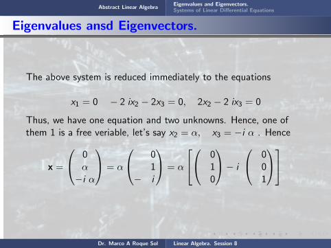
Abstract Linear AlgebraEigenvalues and Eigenvectors.Systems of Linear Differential Equations
Eigenvalues ansd Eigenvectors.
The above system is reduced immediately to the equations
x1 = 0 − 2 ix2 − 2x3 = 0, 2x2 − 2 ix3 = 0
Thus, we have one equation and two unknowns. Hence, one ofthem 1 is a free veriable, let’s say x2 = α, x3 = −i α . Hence
x =
0α−i α
= α
01
− i
= α
010
− i
001
Dr. Marco A Roque Sol Linear Algebra. Session 8

Abstract Linear AlgebraEigenvalues and Eigenvectors.Systems of Linear Differential Equations
Eigenvalues ansd Eigenvectors.
In this way, there are two real linearly independent eigenvectorsassociated to λ2 = 1 + 2 i , namely,
x(2) =
010
x(3) =
001
3) For λ3 = 1− 2 i
(A− λ2I) x =
1− λ 0 02 1− λ −23 2 1− λ
x1x2x3
=
2 i 0 02 2 i −23 2 2 i
x1x2x3
=
000
Dr. Marco A Roque Sol Linear Algebra. Session 8

Abstract Linear AlgebraEigenvalues and Eigenvectors.Systems of Linear Differential Equations
Eigenvalues ansd Eigenvectors.
In this way,
there are two real linearly independent eigenvectorsassociated to λ2 = 1 + 2 i , namely,
x(2) =
010
x(3) =
001
3) For λ3 = 1− 2 i
(A− λ2I) x =
1− λ 0 02 1− λ −23 2 1− λ
x1x2x3
=
2 i 0 02 2 i −23 2 2 i
x1x2x3
=
000
Dr. Marco A Roque Sol Linear Algebra. Session 8
Abstract Linear AlgebraEigenvalues and Eigenvectors.Systems of Linear Differential Equations
Eigenvalues ansd Eigenvectors.
In this way, there are two real
linearly independent eigenvectorsassociated to λ2 = 1 + 2 i , namely,
x(2) =
010
x(3) =
001
3) For λ3 = 1− 2 i
(A− λ2I) x =
1− λ 0 02 1− λ −23 2 1− λ
x1x2x3
=
2 i 0 02 2 i −23 2 2 i
x1x2x3
=
000
Dr. Marco A Roque Sol Linear Algebra. Session 8
Abstract Linear AlgebraEigenvalues and Eigenvectors.Systems of Linear Differential Equations
Eigenvalues ansd Eigenvectors.
In this way, there are two real linearly independent
eigenvectorsassociated to λ2 = 1 + 2 i , namely,
x(2) =
010
x(3) =
001
3) For λ3 = 1− 2 i
(A− λ2I) x =
1− λ 0 02 1− λ −23 2 1− λ
x1x2x3
=
2 i 0 02 2 i −23 2 2 i
x1x2x3
=
000
Dr. Marco A Roque Sol Linear Algebra. Session 8
Abstract Linear AlgebraEigenvalues and Eigenvectors.Systems of Linear Differential Equations
Eigenvalues ansd Eigenvectors.
In this way, there are two real linearly independent eigenvectorsassociated
to λ2 = 1 + 2 i , namely,
x(2) =
010
x(3) =
001
3) For λ3 = 1− 2 i
(A− λ2I) x =
1− λ 0 02 1− λ −23 2 1− λ
x1x2x3
=
2 i 0 02 2 i −23 2 2 i
x1x2x3
=
000
Dr. Marco A Roque Sol Linear Algebra. Session 8
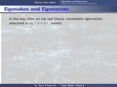
Abstract Linear AlgebraEigenvalues and Eigenvectors.Systems of Linear Differential Equations
Eigenvalues ansd Eigenvectors.
In this way, there are two real linearly independent eigenvectorsassociated to λ2 = 1 + 2 i , namely,
x(2) =
010
x(3) =
001
3) For λ3 = 1− 2 i
(A− λ2I) x =
1− λ 0 02 1− λ −23 2 1− λ
x1x2x3
=
2 i 0 02 2 i −23 2 2 i
x1x2x3
=
000
Dr. Marco A Roque Sol Linear Algebra. Session 8

Abstract Linear AlgebraEigenvalues and Eigenvectors.Systems of Linear Differential Equations
Eigenvalues ansd Eigenvectors.
In this way, there are two real linearly independent eigenvectorsassociated to λ2 = 1 + 2 i , namely,
x(2) =
010
x(3) =
001
3) For λ3 = 1− 2 i
(A− λ2I) x =
1− λ 0 02 1− λ −23 2 1− λ
x1x2x3
=
2 i 0 02 2 i −23 2 2 i
x1x2x3
=
000
Dr. Marco A Roque Sol Linear Algebra. Session 8
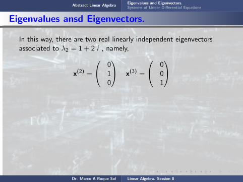
Abstract Linear AlgebraEigenvalues and Eigenvectors.Systems of Linear Differential Equations
Eigenvalues ansd Eigenvectors.
In this way, there are two real linearly independent eigenvectorsassociated to λ2 = 1 + 2 i , namely,
x(2) =
010
x(3) =
001
3) For λ3 = 1− 2 i
(A− λ2I) x =
1− λ 0 02 1− λ −23 2 1− λ
x1x2x3
=
2 i 0 02 2 i −23 2 2 i
x1x2x3
=
000
Dr. Marco A Roque Sol Linear Algebra. Session 8
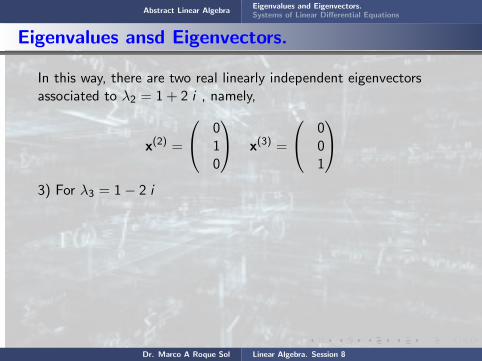
Abstract Linear AlgebraEigenvalues and Eigenvectors.Systems of Linear Differential Equations
Eigenvalues ansd Eigenvectors.
In this way, there are two real linearly independent eigenvectorsassociated to λ2 = 1 + 2 i , namely,
x(2) =
010
x(3) =
001
3) For λ3 = 1− 2 i
(A− λ2I) x =
1− λ 0 02 1− λ −23 2 1− λ
x1x2x3
=
2 i 0 02 2 i −23 2 2 i
x1x2x3
=
000
Dr. Marco A Roque Sol Linear Algebra. Session 8
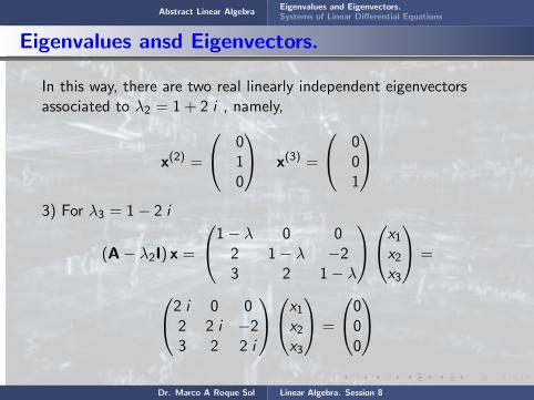
Abstract Linear AlgebraEigenvalues and Eigenvectors.Systems of Linear Differential Equations
Eigenvalues ansd Eigenvectors.
The above system is reduced immediately to the equations
x1 = 0; 2i x2 − 2x3 = 0; 2x2 + 2i x3 = 0
Thus, we have one equation and two unknowns. Hence, one ofthem 1, is a free variable, let’s say x2 = α, x3 = i α . Thus wehave
x =
0αi α
= α
01i
= α
010
+ i
001
Dr. Marco A Roque Sol Linear Algebra. Session 8

Abstract Linear AlgebraEigenvalues and Eigenvectors.Systems of Linear Differential Equations
Eigenvalues ansd Eigenvectors.
The above system
is reduced immediately to the equations
x1 = 0; 2i x2 − 2x3 = 0; 2x2 + 2i x3 = 0
Thus, we have one equation and two unknowns. Hence, one ofthem 1, is a free variable, let’s say x2 = α, x3 = i α . Thus wehave
x =
0αi α
= α
01i
= α
010
+ i
001
Dr. Marco A Roque Sol Linear Algebra. Session 8

Abstract Linear AlgebraEigenvalues and Eigenvectors.Systems of Linear Differential Equations
Eigenvalues ansd Eigenvectors.
The above system is reduced immediately
to the equations
x1 = 0; 2i x2 − 2x3 = 0; 2x2 + 2i x3 = 0
Thus, we have one equation and two unknowns. Hence, one ofthem 1, is a free variable, let’s say x2 = α, x3 = i α . Thus wehave
x =
0αi α
= α
01i
= α
010
+ i
001
Dr. Marco A Roque Sol Linear Algebra. Session 8

Abstract Linear AlgebraEigenvalues and Eigenvectors.Systems of Linear Differential Equations
Eigenvalues ansd Eigenvectors.
The above system is reduced immediately to the equations
x1 = 0; 2i x2 − 2x3 = 0; 2x2 + 2i x3 = 0
Thus, we have one equation and two unknowns. Hence, one ofthem 1, is a free variable, let’s say x2 = α, x3 = i α . Thus wehave
x =
0αi α
= α
01i
= α
010
+ i
001
Dr. Marco A Roque Sol Linear Algebra. Session 8

Abstract Linear AlgebraEigenvalues and Eigenvectors.Systems of Linear Differential Equations
Eigenvalues ansd Eigenvectors.
The above system is reduced immediately to the equations
x1 = 0; 2i x2 − 2x3 = 0; 2x2 + 2i x3 = 0
Thus, we have one equation and two unknowns. Hence, one ofthem 1, is a free variable, let’s say x2 = α, x3 = i α . Thus wehave
x =
0αi α
= α
01i
= α
010
+ i
001
Dr. Marco A Roque Sol Linear Algebra. Session 8
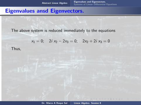
Abstract Linear AlgebraEigenvalues and Eigenvectors.Systems of Linear Differential Equations
Eigenvalues ansd Eigenvectors.
The above system is reduced immediately to the equations
x1 = 0; 2i x2 − 2x3 = 0; 2x2 + 2i x3 = 0
Thus,
we have one equation and two unknowns. Hence, one ofthem 1, is a free variable, let’s say x2 = α, x3 = i α . Thus wehave
x =
0αi α
= α
01i
= α
010
+ i
001
Dr. Marco A Roque Sol Linear Algebra. Session 8

Abstract Linear AlgebraEigenvalues and Eigenvectors.Systems of Linear Differential Equations
Eigenvalues ansd Eigenvectors.
The above system is reduced immediately to the equations
x1 = 0; 2i x2 − 2x3 = 0; 2x2 + 2i x3 = 0
Thus, we have one equation and
two unknowns. Hence, one ofthem 1, is a free variable, let’s say x2 = α, x3 = i α . Thus wehave
x =
0αi α
= α
01i
= α
010
+ i
001
Dr. Marco A Roque Sol Linear Algebra. Session 8

Abstract Linear AlgebraEigenvalues and Eigenvectors.Systems of Linear Differential Equations
Eigenvalues ansd Eigenvectors.
The above system is reduced immediately to the equations
x1 = 0; 2i x2 − 2x3 = 0; 2x2 + 2i x3 = 0
Thus, we have one equation and two unknowns.
Hence, one ofthem 1, is a free variable, let’s say x2 = α, x3 = i α . Thus wehave
x =
0αi α
= α
01i
= α
010
+ i
001
Dr. Marco A Roque Sol Linear Algebra. Session 8

Abstract Linear AlgebraEigenvalues and Eigenvectors.Systems of Linear Differential Equations
Eigenvalues ansd Eigenvectors.
The above system is reduced immediately to the equations
x1 = 0; 2i x2 − 2x3 = 0; 2x2 + 2i x3 = 0
Thus, we have one equation and two unknowns. Hence,
one ofthem 1, is a free variable, let’s say x2 = α, x3 = i α . Thus wehave
x =
0αi α
= α
01i
= α
010
+ i
001
Dr. Marco A Roque Sol Linear Algebra. Session 8

Abstract Linear AlgebraEigenvalues and Eigenvectors.Systems of Linear Differential Equations
Eigenvalues ansd Eigenvectors.
The above system is reduced immediately to the equations
x1 = 0; 2i x2 − 2x3 = 0; 2x2 + 2i x3 = 0
Thus, we have one equation and two unknowns. Hence, one ofthem 1,
is a free variable, let’s say x2 = α, x3 = i α . Thus wehave
x =
0αi α
= α
01i
= α
010
+ i
001
Dr. Marco A Roque Sol Linear Algebra. Session 8
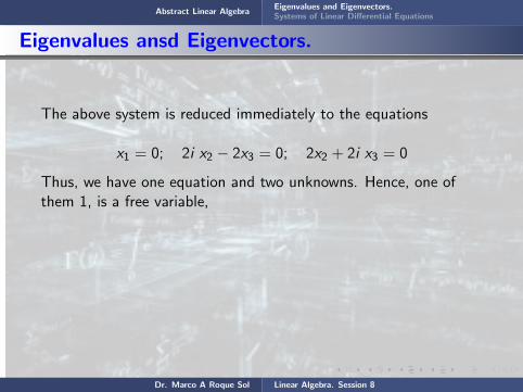
Abstract Linear AlgebraEigenvalues and Eigenvectors.Systems of Linear Differential Equations
Eigenvalues ansd Eigenvectors.
The above system is reduced immediately to the equations
x1 = 0; 2i x2 − 2x3 = 0; 2x2 + 2i x3 = 0
Thus, we have one equation and two unknowns. Hence, one ofthem 1, is a free variable,
let’s say x2 = α, x3 = i α . Thus wehave
x =
0αi α
= α
01i
= α
010
+ i
001
Dr. Marco A Roque Sol Linear Algebra. Session 8

Abstract Linear AlgebraEigenvalues and Eigenvectors.Systems of Linear Differential Equations
Eigenvalues ansd Eigenvectors.
The above system is reduced immediately to the equations
x1 = 0; 2i x2 − 2x3 = 0; 2x2 + 2i x3 = 0
Thus, we have one equation and two unknowns. Hence, one ofthem 1, is a free variable, let’s say x2 = α,
x3 = i α . Thus wehave
x =
0αi α
= α
01i
= α
010
+ i
001
Dr. Marco A Roque Sol Linear Algebra. Session 8

Abstract Linear AlgebraEigenvalues and Eigenvectors.Systems of Linear Differential Equations
Eigenvalues ansd Eigenvectors.
The above system is reduced immediately to the equations
x1 = 0; 2i x2 − 2x3 = 0; 2x2 + 2i x3 = 0
Thus, we have one equation and two unknowns. Hence, one ofthem 1, is a free variable, let’s say x2 = α, x3 = i α .
Thus wehave
x =
0αi α
= α
01i
= α
010
+ i
001
Dr. Marco A Roque Sol Linear Algebra. Session 8

Abstract Linear AlgebraEigenvalues and Eigenvectors.Systems of Linear Differential Equations
Eigenvalues ansd Eigenvectors.
The above system is reduced immediately to the equations
x1 = 0; 2i x2 − 2x3 = 0; 2x2 + 2i x3 = 0
Thus, we have one equation and two unknowns. Hence, one ofthem 1, is a free variable, let’s say x2 = α, x3 = i α . Thus wehave
x =
0αi α
= α
01i
= α
010
+ i
001
Dr. Marco A Roque Sol Linear Algebra. Session 8
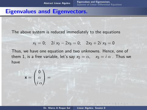
Abstract Linear AlgebraEigenvalues and Eigenvectors.Systems of Linear Differential Equations
Eigenvalues ansd Eigenvectors.
The above system is reduced immediately to the equations
x1 = 0; 2i x2 − 2x3 = 0; 2x2 + 2i x3 = 0
Thus, we have one equation and two unknowns. Hence, one ofthem 1, is a free variable, let’s say x2 = α, x3 = i α . Thus wehave
x =
0αi α
=
α
01i
= α
010
+ i
001
Dr. Marco A Roque Sol Linear Algebra. Session 8

Abstract Linear AlgebraEigenvalues and Eigenvectors.Systems of Linear Differential Equations
Eigenvalues ansd Eigenvectors.
The above system is reduced immediately to the equations
x1 = 0; 2i x2 − 2x3 = 0; 2x2 + 2i x3 = 0
Thus, we have one equation and two unknowns. Hence, one ofthem 1, is a free variable, let’s say x2 = α, x3 = i α . Thus wehave
x =
0αi α
= α
01i
=
α
010
+ i
001
Dr. Marco A Roque Sol Linear Algebra. Session 8

Abstract Linear AlgebraEigenvalues and Eigenvectors.Systems of Linear Differential Equations
Eigenvalues ansd Eigenvectors.
The above system is reduced immediately to the equations
x1 = 0; 2i x2 − 2x3 = 0; 2x2 + 2i x3 = 0
Thus, we have one equation and two unknowns. Hence, one ofthem 1, is a free variable, let’s say x2 = α, x3 = i α . Thus wehave
x =
0αi α
= α
01i
= α
010
+
i
001
Dr. Marco A Roque Sol Linear Algebra. Session 8

Abstract Linear AlgebraEigenvalues and Eigenvectors.Systems of Linear Differential Equations
Eigenvalues ansd Eigenvectors.
The above system is reduced immediately to the equations
x1 = 0; 2i x2 − 2x3 = 0; 2x2 + 2i x3 = 0
Thus, we have one equation and two unknowns. Hence, one ofthem 1, is a free variable, let’s say x2 = α, x3 = i α . Thus wehave
x =
0αi α
= α
01i
= α
010
+ i
001
Dr. Marco A Roque Sol Linear Algebra. Session 8

Abstract Linear AlgebraEigenvalues and Eigenvectors.Systems of Linear Differential Equations
Eigenvalues ansd Eigenvectors.
In this way, there is two real linearly independent eigenvectorsassociated to λ2 = 1 + 2 i , namely,
x(2) =
010
x(3) =
001
Hence, we have three linearly independent eigenvectors, namely
x(1) =
1− 3/2
1
x(2) =
010
x(3) =
001
that is, the matrix A is Non-defective
Dr. Marco A Roque Sol Linear Algebra. Session 8

Abstract Linear AlgebraEigenvalues and Eigenvectors.Systems of Linear Differential Equations
Eigenvalues ansd Eigenvectors.
In this way,
there is two real linearly independent eigenvectorsassociated to λ2 = 1 + 2 i , namely,
x(2) =
010
x(3) =
001
Hence, we have three linearly independent eigenvectors, namely
x(1) =
1− 3/2
1
x(2) =
010
x(3) =
001
that is, the matrix A is Non-defective
Dr. Marco A Roque Sol Linear Algebra. Session 8
Abstract Linear AlgebraEigenvalues and Eigenvectors.Systems of Linear Differential Equations
Eigenvalues ansd Eigenvectors.
In this way, there is
two real linearly independent eigenvectorsassociated to λ2 = 1 + 2 i , namely,
x(2) =
010
x(3) =
001
Hence, we have three linearly independent eigenvectors, namely
x(1) =
1− 3/2
1
x(2) =
010
x(3) =
001
that is, the matrix A is Non-defective
Dr. Marco A Roque Sol Linear Algebra. Session 8
Abstract Linear AlgebraEigenvalues and Eigenvectors.Systems of Linear Differential Equations
Eigenvalues ansd Eigenvectors.
In this way, there is two real
linearly independent eigenvectorsassociated to λ2 = 1 + 2 i , namely,
x(2) =
010
x(3) =
001
Hence, we have three linearly independent eigenvectors, namely
x(1) =
1− 3/2
1
x(2) =
010
x(3) =
001
that is, the matrix A is Non-defective
Dr. Marco A Roque Sol Linear Algebra. Session 8

Abstract Linear AlgebraEigenvalues and Eigenvectors.Systems of Linear Differential Equations
Eigenvalues ansd Eigenvectors.
In this way, there is two real linearly independent
eigenvectorsassociated to λ2 = 1 + 2 i , namely,
x(2) =
010
x(3) =
001
Hence, we have three linearly independent eigenvectors, namely
x(1) =
1− 3/2
1
x(2) =
010
x(3) =
001
that is, the matrix A is Non-defective
Dr. Marco A Roque Sol Linear Algebra. Session 8

Abstract Linear AlgebraEigenvalues and Eigenvectors.Systems of Linear Differential Equations
Eigenvalues ansd Eigenvectors.
In this way, there is two real linearly independent eigenvectorsassociated
to λ2 = 1 + 2 i , namely,
x(2) =
010
x(3) =
001
Hence, we have three linearly independent eigenvectors, namely
x(1) =
1− 3/2
1
x(2) =
010
x(3) =
001
that is, the matrix A is Non-defective
Dr. Marco A Roque Sol Linear Algebra. Session 8

Abstract Linear AlgebraEigenvalues and Eigenvectors.Systems of Linear Differential Equations
Eigenvalues ansd Eigenvectors.
In this way, there is two real linearly independent eigenvectorsassociated to λ2 = 1 + 2 i , namely,
x(2) =
010
x(3) =
001
Hence, we have three linearly independent eigenvectors, namely
x(1) =
1− 3/2
1
x(2) =
010
x(3) =
001
that is, the matrix A is Non-defective
Dr. Marco A Roque Sol Linear Algebra. Session 8

Abstract Linear AlgebraEigenvalues and Eigenvectors.Systems of Linear Differential Equations
Eigenvalues ansd Eigenvectors.
In this way, there is two real linearly independent eigenvectorsassociated to λ2 = 1 + 2 i , namely,
x(2) =
010
x(3) =
001
Hence,
we have three linearly independent eigenvectors, namely
x(1) =
1− 3/2
1
x(2) =
010
x(3) =
001
that is, the matrix A is Non-defective
Dr. Marco A Roque Sol Linear Algebra. Session 8

Abstract Linear AlgebraEigenvalues and Eigenvectors.Systems of Linear Differential Equations
Eigenvalues ansd Eigenvectors.
In this way, there is two real linearly independent eigenvectorsassociated to λ2 = 1 + 2 i , namely,
x(2) =
010
x(3) =
001
Hence, we have three
linearly independent eigenvectors, namely
x(1) =
1− 3/2
1
x(2) =
010
x(3) =
001
that is, the matrix A is Non-defective
Dr. Marco A Roque Sol Linear Algebra. Session 8

Abstract Linear AlgebraEigenvalues and Eigenvectors.Systems of Linear Differential Equations
Eigenvalues ansd Eigenvectors.
In this way, there is two real linearly independent eigenvectorsassociated to λ2 = 1 + 2 i , namely,
x(2) =
010
x(3) =
001
Hence, we have three linearly independent
eigenvectors, namely
x(1) =
1− 3/2
1
x(2) =
010
x(3) =
001
that is, the matrix A is Non-defective
Dr. Marco A Roque Sol Linear Algebra. Session 8
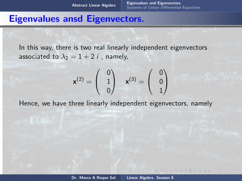
Abstract Linear AlgebraEigenvalues and Eigenvectors.Systems of Linear Differential Equations
Eigenvalues ansd Eigenvectors.
In this way, there is two real linearly independent eigenvectorsassociated to λ2 = 1 + 2 i , namely,
x(2) =
010
x(3) =
001
Hence, we have three linearly independent eigenvectors, namely
x(1) =
1− 3/2
1
x(2) =
010
x(3) =
001
that is, the matrix A is Non-defective
Dr. Marco A Roque Sol Linear Algebra. Session 8

Abstract Linear AlgebraEigenvalues and Eigenvectors.Systems of Linear Differential Equations
Eigenvalues ansd Eigenvectors.
In this way, there is two real linearly independent eigenvectorsassociated to λ2 = 1 + 2 i , namely,
x(2) =
010
x(3) =
001
Hence, we have three linearly independent eigenvectors, namely
x(1) =
1− 3/2
1
x(2) =
010
x(3) =
001
that is, the matrix A is Non-defective
Dr. Marco A Roque Sol Linear Algebra. Session 8
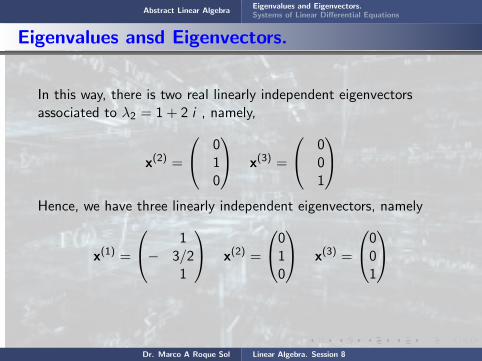
Abstract Linear AlgebraEigenvalues and Eigenvectors.Systems of Linear Differential Equations
Eigenvalues ansd Eigenvectors.
In this way, there is two real linearly independent eigenvectorsassociated to λ2 = 1 + 2 i , namely,
x(2) =
010
x(3) =
001
Hence, we have three linearly independent eigenvectors, namely
x(1) =
1− 3/2
1
x(2) =
010
x(3) =
001
that is,
the matrix A is Non-defective
Dr. Marco A Roque Sol Linear Algebra. Session 8

Abstract Linear AlgebraEigenvalues and Eigenvectors.Systems of Linear Differential Equations
Eigenvalues ansd Eigenvectors.
In this way, there is two real linearly independent eigenvectorsassociated to λ2 = 1 + 2 i , namely,
x(2) =
010
x(3) =
001
Hence, we have three linearly independent eigenvectors, namely
x(1) =
1− 3/2
1
x(2) =
010
x(3) =
001
that is, the matrix A
is Non-defective
Dr. Marco A Roque Sol Linear Algebra. Session 8

Abstract Linear AlgebraEigenvalues and Eigenvectors.Systems of Linear Differential Equations
Eigenvalues ansd Eigenvectors.
In this way, there is two real linearly independent eigenvectorsassociated to λ2 = 1 + 2 i , namely,
x(2) =
010
x(3) =
001
Hence, we have three linearly independent eigenvectors, namely
x(1) =
1− 3/2
1
x(2) =
010
x(3) =
001
that is, the matrix A is Non-defective
Dr. Marco A Roque Sol Linear Algebra. Session 8

Abstract Linear AlgebraEigenvalues and Eigenvectors.Systems of Linear Differential Equations
Eigenvalues ansd Eigenvectors.
OBS
Let A be a real-valued n × n matrix. If x(1) = x(R) ± i x(I ) arecomplex eigenvectors of the matrix A with complex eigenvaluesλ = u ± i v . then, x(R) and x(I ) are two real eigenvectors for Awith eigenvalues λ = u ± i v
Finally, let’s introduce another concept
The Dot Product in Rn
For y = (y1, y2, ..., yn), x = (x1, x2, ..., xn) ∈ R, define the dotproduct or inner product or scalar product.as
Dr. Marco A Roque Sol Linear Algebra. Session 8

Abstract Linear AlgebraEigenvalues and Eigenvectors.Systems of Linear Differential Equations
Eigenvalues ansd Eigenvectors.
OBS
Let A
be a real-valued n × n matrix. If x(1) = x(R) ± i x(I ) arecomplex eigenvectors of the matrix A with complex eigenvaluesλ = u ± i v . then, x(R) and x(I ) are two real eigenvectors for Awith eigenvalues λ = u ± i v
Finally, let’s introduce another concept
The Dot Product in Rn
For y = (y1, y2, ..., yn), x = (x1, x2, ..., xn) ∈ R, define the dotproduct or inner product or scalar product.as
Dr. Marco A Roque Sol Linear Algebra. Session 8

Abstract Linear AlgebraEigenvalues and Eigenvectors.Systems of Linear Differential Equations
Eigenvalues ansd Eigenvectors.
OBS
Let A be a real-valued
n × n matrix. If x(1) = x(R) ± i x(I ) arecomplex eigenvectors of the matrix A with complex eigenvaluesλ = u ± i v . then, x(R) and x(I ) are two real eigenvectors for Awith eigenvalues λ = u ± i v
Finally, let’s introduce another concept
The Dot Product in Rn
For y = (y1, y2, ..., yn), x = (x1, x2, ..., xn) ∈ R, define the dotproduct or inner product or scalar product.as
Dr. Marco A Roque Sol Linear Algebra. Session 8

Abstract Linear AlgebraEigenvalues and Eigenvectors.Systems of Linear Differential Equations
Eigenvalues ansd Eigenvectors.
OBS
Let A be a real-valued n × n matrix.
If x(1) = x(R) ± i x(I ) arecomplex eigenvectors of the matrix A with complex eigenvaluesλ = u ± i v . then, x(R) and x(I ) are two real eigenvectors for Awith eigenvalues λ = u ± i v
Finally, let’s introduce another concept
The Dot Product in Rn
For y = (y1, y2, ..., yn), x = (x1, x2, ..., xn) ∈ R, define the dotproduct or inner product or scalar product.as
Dr. Marco A Roque Sol Linear Algebra. Session 8
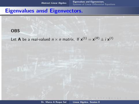
Abstract Linear AlgebraEigenvalues and Eigenvectors.Systems of Linear Differential Equations
Eigenvalues ansd Eigenvectors.
OBS
Let A be a real-valued n × n matrix. If x(1) = x(R) ± i x(I )
arecomplex eigenvectors of the matrix A with complex eigenvaluesλ = u ± i v . then, x(R) and x(I ) are two real eigenvectors for Awith eigenvalues λ = u ± i v
Finally, let’s introduce another concept
The Dot Product in Rn
For y = (y1, y2, ..., yn), x = (x1, x2, ..., xn) ∈ R, define the dotproduct or inner product or scalar product.as
Dr. Marco A Roque Sol Linear Algebra. Session 8

Abstract Linear AlgebraEigenvalues and Eigenvectors.Systems of Linear Differential Equations
Eigenvalues ansd Eigenvectors.
OBS
Let A be a real-valued n × n matrix. If x(1) = x(R) ± i x(I ) arecomplex eigenvectors
of the matrix A with complex eigenvaluesλ = u ± i v . then, x(R) and x(I ) are two real eigenvectors for Awith eigenvalues λ = u ± i v
Finally, let’s introduce another concept
The Dot Product in Rn
For y = (y1, y2, ..., yn), x = (x1, x2, ..., xn) ∈ R, define the dotproduct or inner product or scalar product.as
Dr. Marco A Roque Sol Linear Algebra. Session 8

Abstract Linear AlgebraEigenvalues and Eigenvectors.Systems of Linear Differential Equations
Eigenvalues ansd Eigenvectors.
OBS
Let A be a real-valued n × n matrix. If x(1) = x(R) ± i x(I ) arecomplex eigenvectors of the matrix A
with complex eigenvaluesλ = u ± i v . then, x(R) and x(I ) are two real eigenvectors for Awith eigenvalues λ = u ± i v
Finally, let’s introduce another concept
The Dot Product in Rn
For y = (y1, y2, ..., yn), x = (x1, x2, ..., xn) ∈ R, define the dotproduct or inner product or scalar product.as
Dr. Marco A Roque Sol Linear Algebra. Session 8

Abstract Linear AlgebraEigenvalues and Eigenvectors.Systems of Linear Differential Equations
Eigenvalues ansd Eigenvectors.
OBS
Let A be a real-valued n × n matrix. If x(1) = x(R) ± i x(I ) arecomplex eigenvectors of the matrix A with complex eigenvaluesλ = u ± i v . then,
x(R) and x(I ) are two real eigenvectors for Awith eigenvalues λ = u ± i v
Finally, let’s introduce another concept
The Dot Product in Rn
For y = (y1, y2, ..., yn), x = (x1, x2, ..., xn) ∈ R, define the dotproduct or inner product or scalar product.as
Dr. Marco A Roque Sol Linear Algebra. Session 8

Abstract Linear AlgebraEigenvalues and Eigenvectors.Systems of Linear Differential Equations
Eigenvalues ansd Eigenvectors.
OBS
Let A be a real-valued n × n matrix. If x(1) = x(R) ± i x(I ) arecomplex eigenvectors of the matrix A with complex eigenvaluesλ = u ± i v . then, x(R) and x(I )
are two real eigenvectors for Awith eigenvalues λ = u ± i v
Finally, let’s introduce another concept
The Dot Product in Rn
For y = (y1, y2, ..., yn), x = (x1, x2, ..., xn) ∈ R, define the dotproduct or inner product or scalar product.as
Dr. Marco A Roque Sol Linear Algebra. Session 8
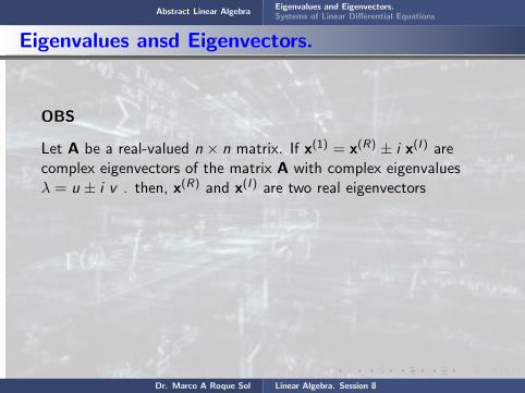
Abstract Linear AlgebraEigenvalues and Eigenvectors.Systems of Linear Differential Equations
Eigenvalues ansd Eigenvectors.
OBS
Let A be a real-valued n × n matrix. If x(1) = x(R) ± i x(I ) arecomplex eigenvectors of the matrix A with complex eigenvaluesλ = u ± i v . then, x(R) and x(I ) are two real eigenvectors
for Awith eigenvalues λ = u ± i v
Finally, let’s introduce another concept
The Dot Product in Rn
For y = (y1, y2, ..., yn), x = (x1, x2, ..., xn) ∈ R, define the dotproduct or inner product or scalar product.as
Dr. Marco A Roque Sol Linear Algebra. Session 8

Abstract Linear AlgebraEigenvalues and Eigenvectors.Systems of Linear Differential Equations
Eigenvalues ansd Eigenvectors.
OBS
Let A be a real-valued n × n matrix. If x(1) = x(R) ± i x(I ) arecomplex eigenvectors of the matrix A with complex eigenvaluesλ = u ± i v . then, x(R) and x(I ) are two real eigenvectors for A
with eigenvalues λ = u ± i v
Finally, let’s introduce another concept
The Dot Product in Rn
For y = (y1, y2, ..., yn), x = (x1, x2, ..., xn) ∈ R, define the dotproduct or inner product or scalar product.as
Dr. Marco A Roque Sol Linear Algebra. Session 8
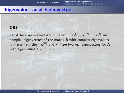
Abstract Linear AlgebraEigenvalues and Eigenvectors.Systems of Linear Differential Equations
Eigenvalues ansd Eigenvectors.
OBS
Let A be a real-valued n × n matrix. If x(1) = x(R) ± i x(I ) arecomplex eigenvectors of the matrix A with complex eigenvaluesλ = u ± i v . then, x(R) and x(I ) are two real eigenvectors for Awith eigenvalues λ = u ± i v
Finally, let’s introduce another concept
The Dot Product in Rn
For y = (y1, y2, ..., yn), x = (x1, x2, ..., xn) ∈ R, define the dotproduct or inner product or scalar product.as
Dr. Marco A Roque Sol Linear Algebra. Session 8

Abstract Linear AlgebraEigenvalues and Eigenvectors.Systems of Linear Differential Equations
Eigenvalues ansd Eigenvectors.
OBS
Let A be a real-valued n × n matrix. If x(1) = x(R) ± i x(I ) arecomplex eigenvectors of the matrix A with complex eigenvaluesλ = u ± i v . then, x(R) and x(I ) are two real eigenvectors for Awith eigenvalues λ = u ± i v
Finally,
let’s introduce another concept
The Dot Product in Rn
For y = (y1, y2, ..., yn), x = (x1, x2, ..., xn) ∈ R, define the dotproduct or inner product or scalar product.as
Dr. Marco A Roque Sol Linear Algebra. Session 8

Abstract Linear AlgebraEigenvalues and Eigenvectors.Systems of Linear Differential Equations
Eigenvalues ansd Eigenvectors.
OBS
Let A be a real-valued n × n matrix. If x(1) = x(R) ± i x(I ) arecomplex eigenvectors of the matrix A with complex eigenvaluesλ = u ± i v . then, x(R) and x(I ) are two real eigenvectors for Awith eigenvalues λ = u ± i v
Finally, let’s introduce
another concept
The Dot Product in Rn
For y = (y1, y2, ..., yn), x = (x1, x2, ..., xn) ∈ R, define the dotproduct or inner product or scalar product.as
Dr. Marco A Roque Sol Linear Algebra. Session 8

Abstract Linear AlgebraEigenvalues and Eigenvectors.Systems of Linear Differential Equations
Eigenvalues ansd Eigenvectors.
OBS
Let A be a real-valued n × n matrix. If x(1) = x(R) ± i x(I ) arecomplex eigenvectors of the matrix A with complex eigenvaluesλ = u ± i v . then, x(R) and x(I ) are two real eigenvectors for Awith eigenvalues λ = u ± i v
Finally, let’s introduce another concept
The Dot Product in Rn
For y = (y1, y2, ..., yn), x = (x1, x2, ..., xn) ∈ R, define the dotproduct or inner product or scalar product.as
Dr. Marco A Roque Sol Linear Algebra. Session 8
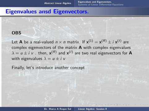
Abstract Linear AlgebraEigenvalues and Eigenvectors.Systems of Linear Differential Equations
Eigenvalues ansd Eigenvectors.
OBS
Let A be a real-valued n × n matrix. If x(1) = x(R) ± i x(I ) arecomplex eigenvectors of the matrix A with complex eigenvaluesλ = u ± i v . then, x(R) and x(I ) are two real eigenvectors for Awith eigenvalues λ = u ± i v
Finally, let’s introduce another concept
The Dot Product in Rn
For y = (y1, y2, ..., yn), x = (x1, x2, ..., xn) ∈ R, define the dotproduct or inner product or scalar product.as
Dr. Marco A Roque Sol Linear Algebra. Session 8
Abstract Linear AlgebraEigenvalues and Eigenvectors.Systems of Linear Differential Equations
Eigenvalues ansd Eigenvectors.
OBS
Let A be a real-valued n × n matrix. If x(1) = x(R) ± i x(I ) arecomplex eigenvectors of the matrix A with complex eigenvaluesλ = u ± i v . then, x(R) and x(I ) are two real eigenvectors for Awith eigenvalues λ = u ± i v
Finally, let’s introduce another concept
The Dot Product in Rn
For
y = (y1, y2, ..., yn), x = (x1, x2, ..., xn) ∈ R, define the dotproduct or inner product or scalar product.as
Dr. Marco A Roque Sol Linear Algebra. Session 8
Abstract Linear AlgebraEigenvalues and Eigenvectors.Systems of Linear Differential Equations
Eigenvalues ansd Eigenvectors.
OBS
Let A be a real-valued n × n matrix. If x(1) = x(R) ± i x(I ) arecomplex eigenvectors of the matrix A with complex eigenvaluesλ = u ± i v . then, x(R) and x(I ) are two real eigenvectors for Awith eigenvalues λ = u ± i v
Finally, let’s introduce another concept
The Dot Product in Rn
For y = (y1, y2, ..., yn), x = (x1, x2, ..., xn) ∈ R,
define the dotproduct or inner product or scalar product.as
Dr. Marco A Roque Sol Linear Algebra. Session 8

Abstract Linear AlgebraEigenvalues and Eigenvectors.Systems of Linear Differential Equations
Eigenvalues ansd Eigenvectors.
OBS
Let A be a real-valued n × n matrix. If x(1) = x(R) ± i x(I ) arecomplex eigenvectors of the matrix A with complex eigenvaluesλ = u ± i v . then, x(R) and x(I ) are two real eigenvectors for Awith eigenvalues λ = u ± i v
Finally, let’s introduce another concept
The Dot Product in Rn
For y = (y1, y2, ..., yn), x = (x1, x2, ..., xn) ∈ R, define the dotproduct
or inner product or scalar product.as
Dr. Marco A Roque Sol Linear Algebra. Session 8
Abstract Linear AlgebraEigenvalues and Eigenvectors.Systems of Linear Differential Equations
Eigenvalues ansd Eigenvectors.
OBS
Let A be a real-valued n × n matrix. If x(1) = x(R) ± i x(I ) arecomplex eigenvectors of the matrix A with complex eigenvaluesλ = u ± i v . then, x(R) and x(I ) are two real eigenvectors for Awith eigenvalues λ = u ± i v
Finally, let’s introduce another concept
The Dot Product in Rn
For y = (y1, y2, ..., yn), x = (x1, x2, ..., xn) ∈ R, define the dotproduct or inner product or
scalar product.as
Dr. Marco A Roque Sol Linear Algebra. Session 8

Abstract Linear AlgebraEigenvalues and Eigenvectors.Systems of Linear Differential Equations
Eigenvalues ansd Eigenvectors.
OBS
Let A be a real-valued n × n matrix. If x(1) = x(R) ± i x(I ) arecomplex eigenvectors of the matrix A with complex eigenvaluesλ = u ± i v . then, x(R) and x(I ) are two real eigenvectors for Awith eigenvalues λ = u ± i v
Finally, let’s introduce another concept
The Dot Product in Rn
For y = (y1, y2, ..., yn), x = (x1, x2, ..., xn) ∈ R, define the dotproduct or inner product or scalar product.as
Dr. Marco A Roque Sol Linear Algebra. Session 8

Abstract Linear AlgebraEigenvalues and Eigenvectors.Systems of Linear Differential Equations
Eigenvalues ansd Eigenvectors.
x · y = < x, y >=(x1 x2 . . . xn
)y1y2...yn
= x1y1 + x2y2 + ...+ xnyn
OBS
a) x and y are said to be orthogonal if < x, y >= 0 .
b) Orthogonal nonzero vectors are linearly independent.
Dr. Marco A Roque Sol Linear Algebra. Session 8

Abstract Linear AlgebraEigenvalues and Eigenvectors.Systems of Linear Differential Equations
Eigenvalues ansd Eigenvectors.
x · y =
< x, y >=(x1 x2 . . . xn
)y1y2...yn
= x1y1 + x2y2 + ...+ xnyn
OBS
a) x and y are said to be orthogonal if < x, y >= 0 .
b) Orthogonal nonzero vectors are linearly independent.
Dr. Marco A Roque Sol Linear Algebra. Session 8

Abstract Linear AlgebraEigenvalues and Eigenvectors.Systems of Linear Differential Equations
Eigenvalues ansd Eigenvectors.
x · y = < x, y >=
(x1 x2 . . . xn
)y1y2...yn
= x1y1 + x2y2 + ...+ xnyn
OBS
a) x and y are said to be orthogonal if < x, y >= 0 .
b) Orthogonal nonzero vectors are linearly independent.
Dr. Marco A Roque Sol Linear Algebra. Session 8
Abstract Linear AlgebraEigenvalues and Eigenvectors.Systems of Linear Differential Equations
Eigenvalues ansd Eigenvectors.
x · y = < x, y >=(x1 x2 . . . xn
)
y1y2...yn
= x1y1 + x2y2 + ...+ xnyn
OBS
a) x and y are said to be orthogonal if < x, y >= 0 .
b) Orthogonal nonzero vectors are linearly independent.
Dr. Marco A Roque Sol Linear Algebra. Session 8

Abstract Linear AlgebraEigenvalues and Eigenvectors.Systems of Linear Differential Equations
Eigenvalues ansd Eigenvectors.
x · y = < x, y >=(x1 x2 . . . xn
)y1y2...yn
=
x1y1 + x2y2 + ...+ xnyn
OBS
a) x and y are said to be orthogonal if < x, y >= 0 .
b) Orthogonal nonzero vectors are linearly independent.
Dr. Marco A Roque Sol Linear Algebra. Session 8

Abstract Linear AlgebraEigenvalues and Eigenvectors.Systems of Linear Differential Equations
Eigenvalues ansd Eigenvectors.
x · y = < x, y >=(x1 x2 . . . xn
)y1y2...yn
= x1y1 + x2y2 + ...+ xnyn
OBS
a) x and y are said to be orthogonal if < x, y >= 0 .
b) Orthogonal nonzero vectors are linearly independent.
Dr. Marco A Roque Sol Linear Algebra. Session 8
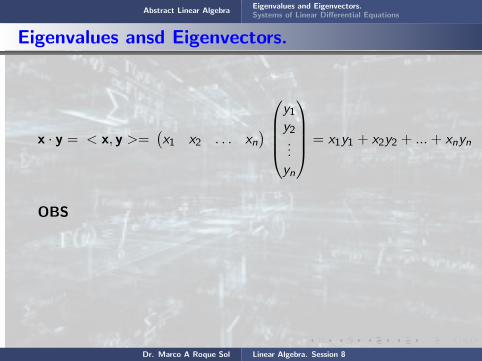
Abstract Linear AlgebraEigenvalues and Eigenvectors.Systems of Linear Differential Equations
Eigenvalues ansd Eigenvectors.
x · y = < x, y >=(x1 x2 . . . xn
)y1y2...yn
= x1y1 + x2y2 + ...+ xnyn
OBS
a) x and y
are said to be orthogonal if < x, y >= 0 .
b) Orthogonal nonzero vectors are linearly independent.
Dr. Marco A Roque Sol Linear Algebra. Session 8
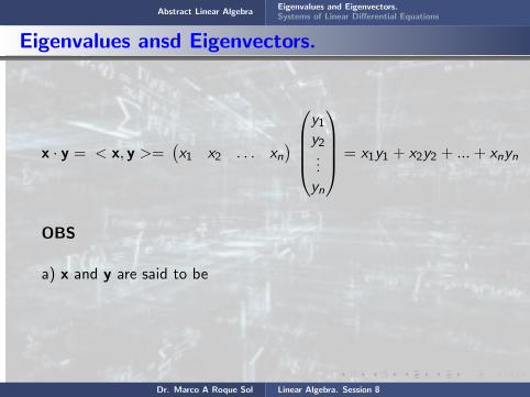
Abstract Linear AlgebraEigenvalues and Eigenvectors.Systems of Linear Differential Equations
Eigenvalues ansd Eigenvectors.
x · y = < x, y >=(x1 x2 . . . xn
)y1y2...yn
= x1y1 + x2y2 + ...+ xnyn
OBS
a) x and y are said to be
orthogonal if < x, y >= 0 .
b) Orthogonal nonzero vectors are linearly independent.
Dr. Marco A Roque Sol Linear Algebra. Session 8

Abstract Linear AlgebraEigenvalues and Eigenvectors.Systems of Linear Differential Equations
Eigenvalues ansd Eigenvectors.
x · y = < x, y >=(x1 x2 . . . xn
)y1y2...yn
= x1y1 + x2y2 + ...+ xnyn
OBS
a) x and y are said to be orthogonal
if < x, y >= 0 .
b) Orthogonal nonzero vectors are linearly independent.
Dr. Marco A Roque Sol Linear Algebra. Session 8
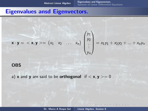
Abstract Linear AlgebraEigenvalues and Eigenvectors.Systems of Linear Differential Equations
Eigenvalues ansd Eigenvectors.
x · y = < x, y >=(x1 x2 . . . xn
)y1y2...yn
= x1y1 + x2y2 + ...+ xnyn
OBS
a) x and y are said to be orthogonal if < x, y >= 0 .
b) Orthogonal nonzero vectors are linearly independent.
Dr. Marco A Roque Sol Linear Algebra. Session 8
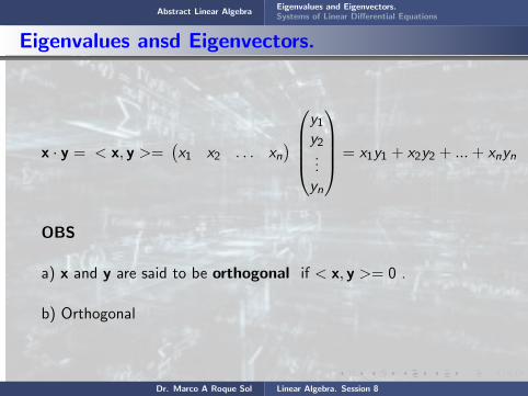
Abstract Linear AlgebraEigenvalues and Eigenvectors.Systems of Linear Differential Equations
Eigenvalues ansd Eigenvectors.
x · y = < x, y >=(x1 x2 . . . xn
)y1y2...yn
= x1y1 + x2y2 + ...+ xnyn
OBS
a) x and y are said to be orthogonal if < x, y >= 0 .
b) Orthogonal
nonzero vectors are linearly independent.
Dr. Marco A Roque Sol Linear Algebra. Session 8

Abstract Linear AlgebraEigenvalues and Eigenvectors.Systems of Linear Differential Equations
Eigenvalues ansd Eigenvectors.
x · y = < x, y >=(x1 x2 . . . xn
)y1y2...yn
= x1y1 + x2y2 + ...+ xnyn
OBS
a) x and y are said to be orthogonal if < x, y >= 0 .
b) Orthogonal nonzero vectors
are linearly independent.
Dr. Marco A Roque Sol Linear Algebra. Session 8
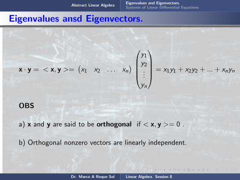
Abstract Linear AlgebraEigenvalues and Eigenvectors.Systems of Linear Differential Equations
Eigenvalues ansd Eigenvectors.
x · y = < x, y >=(x1 x2 . . . xn
)y1y2...yn
= x1y1 + x2y2 + ...+ xnyn
OBS
a) x and y are said to be orthogonal if < x, y >= 0 .
b) Orthogonal nonzero vectors are linearly independent.
Dr. Marco A Roque Sol Linear Algebra. Session 8

Abstract Linear AlgebraEigenvalues and Eigenvectors.Systems of Linear Differential Equations
Eigenvalues ansd Eigenvectors.
Theorem
Let A be an n × n matrix. If A is symetric,( A = AT ) then
1) All eigenvalues are real.
2) A is always Nondefective.
3) The eigenvectors corresponding to different eigenvalues areorthogonal, thus if λ1, λ2, ..., λn are all simple, v1, v2, ..., vn forman orthogonal set.
Dr. Marco A Roque Sol Linear Algebra. Session 8
Abstract Linear AlgebraEigenvalues and Eigenvectors.Systems of Linear Differential Equations
Eigenvalues ansd Eigenvectors.
Theorem
Let A
be an n × n matrix. If A is symetric,( A = AT ) then
1) All eigenvalues are real.
2) A is always Nondefective.
3) The eigenvectors corresponding to different eigenvalues areorthogonal, thus if λ1, λ2, ..., λn are all simple, v1, v2, ..., vn forman orthogonal set.
Dr. Marco A Roque Sol Linear Algebra. Session 8

Abstract Linear AlgebraEigenvalues and Eigenvectors.Systems of Linear Differential Equations
Eigenvalues ansd Eigenvectors.
Theorem
Let A be an n × n matrix.
If A is symetric,( A = AT ) then
1) All eigenvalues are real.
2) A is always Nondefective.
3) The eigenvectors corresponding to different eigenvalues areorthogonal, thus if λ1, λ2, ..., λn are all simple, v1, v2, ..., vn forman orthogonal set.
Dr. Marco A Roque Sol Linear Algebra. Session 8
Abstract Linear AlgebraEigenvalues and Eigenvectors.Systems of Linear Differential Equations
Eigenvalues ansd Eigenvectors.
Theorem
Let A be an n × n matrix. If A
is symetric,( A = AT ) then
1) All eigenvalues are real.
2) A is always Nondefective.
3) The eigenvectors corresponding to different eigenvalues areorthogonal, thus if λ1, λ2, ..., λn are all simple, v1, v2, ..., vn forman orthogonal set.
Dr. Marco A Roque Sol Linear Algebra. Session 8

Abstract Linear AlgebraEigenvalues and Eigenvectors.Systems of Linear Differential Equations
Eigenvalues ansd Eigenvectors.
Theorem
Let A be an n × n matrix. If A is symetric,
( A = AT ) then
1) All eigenvalues are real.
2) A is always Nondefective.
3) The eigenvectors corresponding to different eigenvalues areorthogonal, thus if λ1, λ2, ..., λn are all simple, v1, v2, ..., vn forman orthogonal set.
Dr. Marco A Roque Sol Linear Algebra. Session 8

Abstract Linear AlgebraEigenvalues and Eigenvectors.Systems of Linear Differential Equations
Eigenvalues ansd Eigenvectors.
Theorem
Let A be an n × n matrix. If A is symetric,( A = AT ) then
1) All eigenvalues are real.
2) A is always Nondefective.
3) The eigenvectors corresponding to different eigenvalues areorthogonal, thus if λ1, λ2, ..., λn are all simple, v1, v2, ..., vn forman orthogonal set.
Dr. Marco A Roque Sol Linear Algebra. Session 8
Abstract Linear AlgebraEigenvalues and Eigenvectors.Systems of Linear Differential Equations
Eigenvalues ansd Eigenvectors.
Theorem
Let A be an n × n matrix. If A is symetric,( A = AT ) then
1) All eigenvalues are real.
2) A is always Nondefective.
3) The eigenvectors corresponding to different eigenvalues areorthogonal, thus if λ1, λ2, ..., λn are all simple, v1, v2, ..., vn forman orthogonal set.
Dr. Marco A Roque Sol Linear Algebra. Session 8

Abstract Linear AlgebraEigenvalues and Eigenvectors.Systems of Linear Differential Equations
Eigenvalues ansd Eigenvectors.
Theorem
Let A be an n × n matrix. If A is symetric,( A = AT ) then
1) All eigenvalues are real.
2) A is always Nondefective.
3) The eigenvectors
corresponding to different eigenvalues areorthogonal, thus if λ1, λ2, ..., λn are all simple, v1, v2, ..., vn forman orthogonal set.
Dr. Marco A Roque Sol Linear Algebra. Session 8

Abstract Linear AlgebraEigenvalues and Eigenvectors.Systems of Linear Differential Equations
Eigenvalues ansd Eigenvectors.
Theorem
Let A be an n × n matrix. If A is symetric,( A = AT ) then
1) All eigenvalues are real.
2) A is always Nondefective.
3) The eigenvectors corresponding to
different eigenvalues areorthogonal, thus if λ1, λ2, ..., λn are all simple, v1, v2, ..., vn forman orthogonal set.
Dr. Marco A Roque Sol Linear Algebra. Session 8

Abstract Linear AlgebraEigenvalues and Eigenvectors.Systems of Linear Differential Equations
Eigenvalues ansd Eigenvectors.
Theorem
Let A be an n × n matrix. If A is symetric,( A = AT ) then
1) All eigenvalues are real.
2) A is always Nondefective.
3) The eigenvectors corresponding to different eigenvalues
areorthogonal, thus if λ1, λ2, ..., λn are all simple, v1, v2, ..., vn forman orthogonal set.
Dr. Marco A Roque Sol Linear Algebra. Session 8

Abstract Linear AlgebraEigenvalues and Eigenvectors.Systems of Linear Differential Equations
Eigenvalues ansd Eigenvectors.
Theorem
Let A be an n × n matrix. If A is symetric,( A = AT ) then
1) All eigenvalues are real.
2) A is always Nondefective.
3) The eigenvectors corresponding to different eigenvalues areorthogonal, thus
if λ1, λ2, ..., λn are all simple, v1, v2, ..., vn forman orthogonal set.
Dr. Marco A Roque Sol Linear Algebra. Session 8

Abstract Linear AlgebraEigenvalues and Eigenvectors.Systems of Linear Differential Equations
Eigenvalues ansd Eigenvectors.
Theorem
Let A be an n × n matrix. If A is symetric,( A = AT ) then
1) All eigenvalues are real.
2) A is always Nondefective.
3) The eigenvectors corresponding to different eigenvalues areorthogonal, thus if λ1, λ2, ..., λn
are all simple, v1, v2, ..., vn forman orthogonal set.
Dr. Marco A Roque Sol Linear Algebra. Session 8
Abstract Linear AlgebraEigenvalues and Eigenvectors.Systems of Linear Differential Equations
Eigenvalues ansd Eigenvectors.
Theorem
Let A be an n × n matrix. If A is symetric,( A = AT ) then
1) All eigenvalues are real.
2) A is always Nondefective.
3) The eigenvectors corresponding to different eigenvalues areorthogonal, thus if λ1, λ2, ..., λn are all simple,
v1, v2, ..., vn forman orthogonal set.
Dr. Marco A Roque Sol Linear Algebra. Session 8
Abstract Linear AlgebraEigenvalues and Eigenvectors.Systems of Linear Differential Equations
Eigenvalues ansd Eigenvectors.
Theorem
Let A be an n × n matrix. If A is symetric,( A = AT ) then
1) All eigenvalues are real.
2) A is always Nondefective.
3) The eigenvectors corresponding to different eigenvalues areorthogonal, thus if λ1, λ2, ..., λn are all simple, v1, v2, ..., vn forman orthogonal set.
Dr. Marco A Roque Sol Linear Algebra. Session 8

Abstract Linear AlgebraEigenvalues and Eigenvectors.Systems of Linear Differential Equations
Systems of Linear Differential Equations.
The general theory of a system of n first order linear equations
x ′1 = p11x1 + p12x2 + . . .+ p1nxn + g1(t)x ′2 = p21x1 + p22x2 + . . .+ p2nxn + g2(t)...
...x ′n = pn1x1 + pn2x2 + . . .+ pnnxn + gn(t)
or
X′ = P(t)X + g(t)
closely parallels that of a single linear equation of nth order.
Dr. Marco A Roque Sol Linear Algebra. Session 8
Abstract Linear AlgebraEigenvalues and Eigenvectors.Systems of Linear Differential Equations
Systems of Linear Differential Equations.
The general theory
of a system of n first order linear equations
x ′1 = p11x1 + p12x2 + . . .+ p1nxn + g1(t)x ′2 = p21x1 + p22x2 + . . .+ p2nxn + g2(t)...
...x ′n = pn1x1 + pn2x2 + . . .+ pnnxn + gn(t)
or
X′ = P(t)X + g(t)
closely parallels that of a single linear equation of nth order.
Dr. Marco A Roque Sol Linear Algebra. Session 8

Abstract Linear AlgebraEigenvalues and Eigenvectors.Systems of Linear Differential Equations
Systems of Linear Differential Equations.
The general theory of a system
of n first order linear equations
x ′1 = p11x1 + p12x2 + . . .+ p1nxn + g1(t)x ′2 = p21x1 + p22x2 + . . .+ p2nxn + g2(t)...
...x ′n = pn1x1 + pn2x2 + . . .+ pnnxn + gn(t)
or
X′ = P(t)X + g(t)
closely parallels that of a single linear equation of nth order.
Dr. Marco A Roque Sol Linear Algebra. Session 8

Abstract Linear AlgebraEigenvalues and Eigenvectors.Systems of Linear Differential Equations
Systems of Linear Differential Equations.
The general theory of a system of n first order
linear equations
x ′1 = p11x1 + p12x2 + . . .+ p1nxn + g1(t)x ′2 = p21x1 + p22x2 + . . .+ p2nxn + g2(t)...
...x ′n = pn1x1 + pn2x2 + . . .+ pnnxn + gn(t)
or
X′ = P(t)X + g(t)
closely parallels that of a single linear equation of nth order.
Dr. Marco A Roque Sol Linear Algebra. Session 8
Abstract Linear AlgebraEigenvalues and Eigenvectors.Systems of Linear Differential Equations
Systems of Linear Differential Equations.
The general theory of a system of n first order linear equations
x ′1 = p11x1 + p12x2 + . . .+ p1nxn + g1(t)x ′2 = p21x1 + p22x2 + . . .+ p2nxn + g2(t)...
...x ′n = pn1x1 + pn2x2 + . . .+ pnnxn + gn(t)
or
X′ = P(t)X + g(t)
closely parallels that of a single linear equation of nth order.
Dr. Marco A Roque Sol Linear Algebra. Session 8

Abstract Linear AlgebraEigenvalues and Eigenvectors.Systems of Linear Differential Equations
Systems of Linear Differential Equations.
The general theory of a system of n first order linear equations
x ′1 = p11x1 + p12x2 + . . .+ p1nxn + g1(t)x ′2 = p21x1 + p22x2 + . . .+ p2nxn + g2(t)...
...x ′n = pn1x1 + pn2x2 + . . .+ pnnxn + gn(t)
or
X′ = P(t)X + g(t)
closely parallels
that of a single linear equation of nth order.
Dr. Marco A Roque Sol Linear Algebra. Session 8
Abstract Linear AlgebraEigenvalues and Eigenvectors.Systems of Linear Differential Equations
Systems of Linear Differential Equations.
The general theory of a system of n first order linear equations
x ′1 = p11x1 + p12x2 + . . .+ p1nxn + g1(t)x ′2 = p21x1 + p22x2 + . . .+ p2nxn + g2(t)...
...x ′n = pn1x1 + pn2x2 + . . .+ pnnxn + gn(t)
or
X′ = P(t)X + g(t)
closely parallels that of a single
linear equation of nth order.
Dr. Marco A Roque Sol Linear Algebra. Session 8

Abstract Linear AlgebraEigenvalues and Eigenvectors.Systems of Linear Differential Equations
Systems of Linear Differential Equations.
The general theory of a system of n first order linear equations
x ′1 = p11x1 + p12x2 + . . .+ p1nxn + g1(t)x ′2 = p21x1 + p22x2 + . . .+ p2nxn + g2(t)...
...x ′n = pn1x1 + pn2x2 + . . .+ pnnxn + gn(t)
or
X′ = P(t)X + g(t)
closely parallels that of a single linear equation
of nth order.
Dr. Marco A Roque Sol Linear Algebra. Session 8
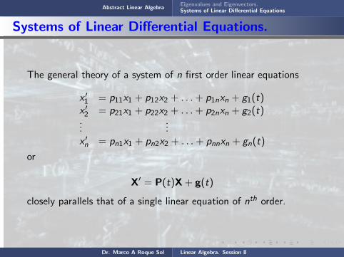
Abstract Linear AlgebraEigenvalues and Eigenvectors.Systems of Linear Differential Equations
Systems of Linear Differential Equations.
The general theory of a system of n first order linear equations
x ′1 = p11x1 + p12x2 + . . .+ p1nxn + g1(t)x ′2 = p21x1 + p22x2 + . . .+ p2nxn + g2(t)...
...x ′n = pn1x1 + pn2x2 + . . .+ pnnxn + gn(t)
or
X′ = P(t)X + g(t)
closely parallels that of a single linear equation of nth order.
Dr. Marco A Roque Sol Linear Algebra. Session 8

Abstract Linear AlgebraEigenvalues and Eigenvectors.Systems of Linear Differential Equations
Systems of Linear Differential Equations.
we assume that P and g are continuous on some intervalα < t < β; that is, each of the scalar functionsp11, ..., pnn, g1, ..., gn is continuous there.
Theorem
If the vector functions x(1) and x(2) are solutions of thehomogeneus system ( g(t) = 0 ) then the linear combinationc1x(1) + c2x(2) is also a solution for any constants c1 and c2.
This is the principle of superposition
Dr. Marco A Roque Sol Linear Algebra. Session 8
Abstract Linear AlgebraEigenvalues and Eigenvectors.Systems of Linear Differential Equations
Systems of Linear Differential Equations.
we assume that
P and g are continuous on some intervalα < t < β; that is, each of the scalar functionsp11, ..., pnn, g1, ..., gn is continuous there.
Theorem
If the vector functions x(1) and x(2) are solutions of thehomogeneus system ( g(t) = 0 ) then the linear combinationc1x(1) + c2x(2) is also a solution for any constants c1 and c2.
This is the principle of superposition
Dr. Marco A Roque Sol Linear Algebra. Session 8
Abstract Linear AlgebraEigenvalues and Eigenvectors.Systems of Linear Differential Equations
Systems of Linear Differential Equations.
we assume that P and g
are continuous on some intervalα < t < β; that is, each of the scalar functionsp11, ..., pnn, g1, ..., gn is continuous there.
Theorem
If the vector functions x(1) and x(2) are solutions of thehomogeneus system ( g(t) = 0 ) then the linear combinationc1x(1) + c2x(2) is also a solution for any constants c1 and c2.
This is the principle of superposition
Dr. Marco A Roque Sol Linear Algebra. Session 8

Abstract Linear AlgebraEigenvalues and Eigenvectors.Systems of Linear Differential Equations
Systems of Linear Differential Equations.
we assume that P and g are continuous
on some intervalα < t < β; that is, each of the scalar functionsp11, ..., pnn, g1, ..., gn is continuous there.
Theorem
If the vector functions x(1) and x(2) are solutions of thehomogeneus system ( g(t) = 0 ) then the linear combinationc1x(1) + c2x(2) is also a solution for any constants c1 and c2.
This is the principle of superposition
Dr. Marco A Roque Sol Linear Algebra. Session 8
Abstract Linear AlgebraEigenvalues and Eigenvectors.Systems of Linear Differential Equations
Systems of Linear Differential Equations.
we assume that P and g are continuous on some interval
α < t < β; that is, each of the scalar functionsp11, ..., pnn, g1, ..., gn is continuous there.
Theorem
If the vector functions x(1) and x(2) are solutions of thehomogeneus system ( g(t) = 0 ) then the linear combinationc1x(1) + c2x(2) is also a solution for any constants c1 and c2.
This is the principle of superposition
Dr. Marco A Roque Sol Linear Algebra. Session 8
Abstract Linear AlgebraEigenvalues and Eigenvectors.Systems of Linear Differential Equations
Systems of Linear Differential Equations.
we assume that P and g are continuous on some intervalα < t < β;
that is, each of the scalar functionsp11, ..., pnn, g1, ..., gn is continuous there.
Theorem
If the vector functions x(1) and x(2) are solutions of thehomogeneus system ( g(t) = 0 ) then the linear combinationc1x(1) + c2x(2) is also a solution for any constants c1 and c2.
This is the principle of superposition
Dr. Marco A Roque Sol Linear Algebra. Session 8

Abstract Linear AlgebraEigenvalues and Eigenvectors.Systems of Linear Differential Equations
Systems of Linear Differential Equations.
we assume that P and g are continuous on some intervalα < t < β; that is,
each of the scalar functionsp11, ..., pnn, g1, ..., gn is continuous there.
Theorem
If the vector functions x(1) and x(2) are solutions of thehomogeneus system ( g(t) = 0 ) then the linear combinationc1x(1) + c2x(2) is also a solution for any constants c1 and c2.
This is the principle of superposition
Dr. Marco A Roque Sol Linear Algebra. Session 8

Abstract Linear AlgebraEigenvalues and Eigenvectors.Systems of Linear Differential Equations
Systems of Linear Differential Equations.
we assume that P and g are continuous on some intervalα < t < β; that is, each of
the scalar functionsp11, ..., pnn, g1, ..., gn is continuous there.
Theorem
If the vector functions x(1) and x(2) are solutions of thehomogeneus system ( g(t) = 0 ) then the linear combinationc1x(1) + c2x(2) is also a solution for any constants c1 and c2.
This is the principle of superposition
Dr. Marco A Roque Sol Linear Algebra. Session 8
Abstract Linear AlgebraEigenvalues and Eigenvectors.Systems of Linear Differential Equations
Systems of Linear Differential Equations.
we assume that P and g are continuous on some intervalα < t < β; that is, each of the scalar functions
p11, ..., pnn, g1, ..., gn is continuous there.
Theorem
If the vector functions x(1) and x(2) are solutions of thehomogeneus system ( g(t) = 0 ) then the linear combinationc1x(1) + c2x(2) is also a solution for any constants c1 and c2.
This is the principle of superposition
Dr. Marco A Roque Sol Linear Algebra. Session 8

Abstract Linear AlgebraEigenvalues and Eigenvectors.Systems of Linear Differential Equations
Systems of Linear Differential Equations.
we assume that P and g are continuous on some intervalα < t < β; that is, each of the scalar functionsp11, ..., pnn, g1, ..., gn
is continuous there.
Theorem
If the vector functions x(1) and x(2) are solutions of thehomogeneus system ( g(t) = 0 ) then the linear combinationc1x(1) + c2x(2) is also a solution for any constants c1 and c2.
This is the principle of superposition
Dr. Marco A Roque Sol Linear Algebra. Session 8
Abstract Linear AlgebraEigenvalues and Eigenvectors.Systems of Linear Differential Equations
Systems of Linear Differential Equations.
we assume that P and g are continuous on some intervalα < t < β; that is, each of the scalar functionsp11, ..., pnn, g1, ..., gn is continuous there.
Theorem
If the vector functions x(1) and x(2) are solutions of thehomogeneus system ( g(t) = 0 ) then the linear combinationc1x(1) + c2x(2) is also a solution for any constants c1 and c2.
This is the principle of superposition
Dr. Marco A Roque Sol Linear Algebra. Session 8

Abstract Linear AlgebraEigenvalues and Eigenvectors.Systems of Linear Differential Equations
Systems of Linear Differential Equations.
we assume that P and g are continuous on some intervalα < t < β; that is, each of the scalar functionsp11, ..., pnn, g1, ..., gn is continuous there.
Theorem
If
the vector functions x(1) and x(2) are solutions of thehomogeneus system ( g(t) = 0 ) then the linear combinationc1x(1) + c2x(2) is also a solution for any constants c1 and c2.
This is the principle of superposition
Dr. Marco A Roque Sol Linear Algebra. Session 8

Abstract Linear AlgebraEigenvalues and Eigenvectors.Systems of Linear Differential Equations
Systems of Linear Differential Equations.
we assume that P and g are continuous on some intervalα < t < β; that is, each of the scalar functionsp11, ..., pnn, g1, ..., gn is continuous there.
Theorem
If the vector functions
x(1) and x(2) are solutions of thehomogeneus system ( g(t) = 0 ) then the linear combinationc1x(1) + c2x(2) is also a solution for any constants c1 and c2.
This is the principle of superposition
Dr. Marco A Roque Sol Linear Algebra. Session 8

Abstract Linear AlgebraEigenvalues and Eigenvectors.Systems of Linear Differential Equations
Systems of Linear Differential Equations.
we assume that P and g are continuous on some intervalα < t < β; that is, each of the scalar functionsp11, ..., pnn, g1, ..., gn is continuous there.
Theorem
If the vector functions x(1) and x(2)
are solutions of thehomogeneus system ( g(t) = 0 ) then the linear combinationc1x(1) + c2x(2) is also a solution for any constants c1 and c2.
This is the principle of superposition
Dr. Marco A Roque Sol Linear Algebra. Session 8

Abstract Linear AlgebraEigenvalues and Eigenvectors.Systems of Linear Differential Equations
Systems of Linear Differential Equations.
we assume that P and g are continuous on some intervalα < t < β; that is, each of the scalar functionsp11, ..., pnn, g1, ..., gn is continuous there.
Theorem
If the vector functions x(1) and x(2) are solutions
of thehomogeneus system ( g(t) = 0 ) then the linear combinationc1x(1) + c2x(2) is also a solution for any constants c1 and c2.
This is the principle of superposition
Dr. Marco A Roque Sol Linear Algebra. Session 8
Abstract Linear AlgebraEigenvalues and Eigenvectors.Systems of Linear Differential Equations
Systems of Linear Differential Equations.
we assume that P and g are continuous on some intervalα < t < β; that is, each of the scalar functionsp11, ..., pnn, g1, ..., gn is continuous there.
Theorem
If the vector functions x(1) and x(2) are solutions of thehomogeneus system
( g(t) = 0 ) then the linear combinationc1x(1) + c2x(2) is also a solution for any constants c1 and c2.
This is the principle of superposition
Dr. Marco A Roque Sol Linear Algebra. Session 8
Abstract Linear AlgebraEigenvalues and Eigenvectors.Systems of Linear Differential Equations
Systems of Linear Differential Equations.
we assume that P and g are continuous on some intervalα < t < β; that is, each of the scalar functionsp11, ..., pnn, g1, ..., gn is continuous there.
Theorem
If the vector functions x(1) and x(2) are solutions of thehomogeneus system ( g(t) = 0 )
then the linear combinationc1x(1) + c2x(2) is also a solution for any constants c1 and c2.
This is the principle of superposition
Dr. Marco A Roque Sol Linear Algebra. Session 8

Abstract Linear AlgebraEigenvalues and Eigenvectors.Systems of Linear Differential Equations
Systems of Linear Differential Equations.
we assume that P and g are continuous on some intervalα < t < β; that is, each of the scalar functionsp11, ..., pnn, g1, ..., gn is continuous there.
Theorem
If the vector functions x(1) and x(2) are solutions of thehomogeneus system ( g(t) = 0 ) then the linear combination
c1x(1) + c2x(2) is also a solution for any constants c1 and c2.
This is the principle of superposition
Dr. Marco A Roque Sol Linear Algebra. Session 8

Abstract Linear AlgebraEigenvalues and Eigenvectors.Systems of Linear Differential Equations
Systems of Linear Differential Equations.
we assume that P and g are continuous on some intervalα < t < β; that is, each of the scalar functionsp11, ..., pnn, g1, ..., gn is continuous there.
Theorem
If the vector functions x(1) and x(2) are solutions of thehomogeneus system ( g(t) = 0 ) then the linear combinationc1x(1) + c2x(2)
is also a solution for any constants c1 and c2.
This is the principle of superposition
Dr. Marco A Roque Sol Linear Algebra. Session 8

Abstract Linear AlgebraEigenvalues and Eigenvectors.Systems of Linear Differential Equations
Systems of Linear Differential Equations.
we assume that P and g are continuous on some intervalα < t < β; that is, each of the scalar functionsp11, ..., pnn, g1, ..., gn is continuous there.
Theorem
If the vector functions x(1) and x(2) are solutions of thehomogeneus system ( g(t) = 0 ) then the linear combinationc1x(1) + c2x(2) is also
a solution for any constants c1 and c2.
This is the principle of superposition
Dr. Marco A Roque Sol Linear Algebra. Session 8
Abstract Linear AlgebraEigenvalues and Eigenvectors.Systems of Linear Differential Equations
Systems of Linear Differential Equations.
we assume that P and g are continuous on some intervalα < t < β; that is, each of the scalar functionsp11, ..., pnn, g1, ..., gn is continuous there.
Theorem
If the vector functions x(1) and x(2) are solutions of thehomogeneus system ( g(t) = 0 ) then the linear combinationc1x(1) + c2x(2) is also a solution
for any constants c1 and c2.
This is the principle of superposition
Dr. Marco A Roque Sol Linear Algebra. Session 8
Abstract Linear AlgebraEigenvalues and Eigenvectors.Systems of Linear Differential Equations
Systems of Linear Differential Equations.
we assume that P and g are continuous on some intervalα < t < β; that is, each of the scalar functionsp11, ..., pnn, g1, ..., gn is continuous there.
Theorem
If the vector functions x(1) and x(2) are solutions of thehomogeneus system ( g(t) = 0 ) then the linear combinationc1x(1) + c2x(2) is also a solution for any constants c1 and c2.
This is the principle of superposition
Dr. Marco A Roque Sol Linear Algebra. Session 8

Abstract Linear AlgebraEigenvalues and Eigenvectors.Systems of Linear Differential Equations
Systems of Linear Differential Equations.
we assume that P and g are continuous on some intervalα < t < β; that is, each of the scalar functionsp11, ..., pnn, g1, ..., gn is continuous there.
Theorem
If the vector functions x(1) and x(2) are solutions of thehomogeneus system ( g(t) = 0 ) then the linear combinationc1x(1) + c2x(2) is also a solution for any constants c1 and c2.
This is
the principle of superposition
Dr. Marco A Roque Sol Linear Algebra. Session 8
Abstract Linear AlgebraEigenvalues and Eigenvectors.Systems of Linear Differential Equations
Systems of Linear Differential Equations.
we assume that P and g are continuous on some intervalα < t < β; that is, each of the scalar functionsp11, ..., pnn, g1, ..., gn is continuous there.
Theorem
If the vector functions x(1) and x(2) are solutions of thehomogeneus system ( g(t) = 0 ) then the linear combinationc1x(1) + c2x(2) is also a solution for any constants c1 and c2.
This is the principle of superposition
Dr. Marco A Roque Sol Linear Algebra. Session 8

Abstract Linear AlgebraEigenvalues and Eigenvectors.Systems of Linear Differential Equations
Systems of Linear Differential Equations.
By repeated application of Theorem, we can conclude that ifx(1), ..., x(k) are solutions of the homogeneous system, then
c1x(1) + ...+ ckx(k)
is also a solution for any constants c1, ..., ck .
Theorem
If the vector functions x(1), ..., x(n) are linearly independentsolutions of the homogeneous system for each point in the intervalα < t < β, then each solution x = φ(t) of the homogeneoussystem can be expressed as a linear combination of x(1), ..., x(n) inexactly one way.
φ(t) = c1x(1) + ...+ ckx(k)
Dr. Marco A Roque Sol Linear Algebra. Session 8

Abstract Linear AlgebraEigenvalues and Eigenvectors.Systems of Linear Differential Equations
Systems of Linear Differential Equations.
By repeated application
of Theorem, we can conclude that ifx(1), ..., x(k) are solutions of the homogeneous system, then
c1x(1) + ...+ ckx(k)
is also a solution for any constants c1, ..., ck .
Theorem
If the vector functions x(1), ..., x(n) are linearly independentsolutions of the homogeneous system for each point in the intervalα < t < β, then each solution x = φ(t) of the homogeneoussystem can be expressed as a linear combination of x(1), ..., x(n) inexactly one way.
φ(t) = c1x(1) + ...+ ckx(k)
Dr. Marco A Roque Sol Linear Algebra. Session 8
Abstract Linear AlgebraEigenvalues and Eigenvectors.Systems of Linear Differential Equations
Systems of Linear Differential Equations.
By repeated application of Theorem, we can conclude
that ifx(1), ..., x(k) are solutions of the homogeneous system, then
c1x(1) + ...+ ckx(k)
is also a solution for any constants c1, ..., ck .
Theorem
If the vector functions x(1), ..., x(n) are linearly independentsolutions of the homogeneous system for each point in the intervalα < t < β, then each solution x = φ(t) of the homogeneoussystem can be expressed as a linear combination of x(1), ..., x(n) inexactly one way.
φ(t) = c1x(1) + ...+ ckx(k)
Dr. Marco A Roque Sol Linear Algebra. Session 8

Abstract Linear AlgebraEigenvalues and Eigenvectors.Systems of Linear Differential Equations
Systems of Linear Differential Equations.
By repeated application of Theorem, we can conclude that ifx(1), ..., x(k)
are solutions of the homogeneous system, then
c1x(1) + ...+ ckx(k)
is also a solution for any constants c1, ..., ck .
Theorem
If the vector functions x(1), ..., x(n) are linearly independentsolutions of the homogeneous system for each point in the intervalα < t < β, then each solution x = φ(t) of the homogeneoussystem can be expressed as a linear combination of x(1), ..., x(n) inexactly one way.
φ(t) = c1x(1) + ...+ ckx(k)
Dr. Marco A Roque Sol Linear Algebra. Session 8
Abstract Linear AlgebraEigenvalues and Eigenvectors.Systems of Linear Differential Equations
Systems of Linear Differential Equations.
By repeated application of Theorem, we can conclude that ifx(1), ..., x(k) are solutions
of the homogeneous system, then
c1x(1) + ...+ ckx(k)
is also a solution for any constants c1, ..., ck .
Theorem
If the vector functions x(1), ..., x(n) are linearly independentsolutions of the homogeneous system for each point in the intervalα < t < β, then each solution x = φ(t) of the homogeneoussystem can be expressed as a linear combination of x(1), ..., x(n) inexactly one way.
φ(t) = c1x(1) + ...+ ckx(k)
Dr. Marco A Roque Sol Linear Algebra. Session 8

Abstract Linear AlgebraEigenvalues and Eigenvectors.Systems of Linear Differential Equations
Systems of Linear Differential Equations.
By repeated application of Theorem, we can conclude that ifx(1), ..., x(k) are solutions of the homogeneous system,
then
c1x(1) + ...+ ckx(k)
is also a solution for any constants c1, ..., ck .
Theorem
If the vector functions x(1), ..., x(n) are linearly independentsolutions of the homogeneous system for each point in the intervalα < t < β, then each solution x = φ(t) of the homogeneoussystem can be expressed as a linear combination of x(1), ..., x(n) inexactly one way.
φ(t) = c1x(1) + ...+ ckx(k)
Dr. Marco A Roque Sol Linear Algebra. Session 8

Abstract Linear AlgebraEigenvalues and Eigenvectors.Systems of Linear Differential Equations
Systems of Linear Differential Equations.
By repeated application of Theorem, we can conclude that ifx(1), ..., x(k) are solutions of the homogeneous system, then
c1x(1) + ...+ ckx(k)
is also a solution for any constants c1, ..., ck .
Theorem
If the vector functions x(1), ..., x(n) are linearly independentsolutions of the homogeneous system for each point in the intervalα < t < β, then each solution x = φ(t) of the homogeneoussystem can be expressed as a linear combination of x(1), ..., x(n) inexactly one way.
φ(t) = c1x(1) + ...+ ckx(k)
Dr. Marco A Roque Sol Linear Algebra. Session 8
Abstract Linear AlgebraEigenvalues and Eigenvectors.Systems of Linear Differential Equations
Systems of Linear Differential Equations.
By repeated application of Theorem, we can conclude that ifx(1), ..., x(k) are solutions of the homogeneous system, then
c1x(1) + ...+ ckx(k)
is also
a solution for any constants c1, ..., ck .
Theorem
If the vector functions x(1), ..., x(n) are linearly independentsolutions of the homogeneous system for each point in the intervalα < t < β, then each solution x = φ(t) of the homogeneoussystem can be expressed as a linear combination of x(1), ..., x(n) inexactly one way.
φ(t) = c1x(1) + ...+ ckx(k)
Dr. Marco A Roque Sol Linear Algebra. Session 8

Abstract Linear AlgebraEigenvalues and Eigenvectors.Systems of Linear Differential Equations
Systems of Linear Differential Equations.
By repeated application of Theorem, we can conclude that ifx(1), ..., x(k) are solutions of the homogeneous system, then
c1x(1) + ...+ ckx(k)
is also a solution
for any constants c1, ..., ck .
Theorem
If the vector functions x(1), ..., x(n) are linearly independentsolutions of the homogeneous system for each point in the intervalα < t < β, then each solution x = φ(t) of the homogeneoussystem can be expressed as a linear combination of x(1), ..., x(n) inexactly one way.
φ(t) = c1x(1) + ...+ ckx(k)
Dr. Marco A Roque Sol Linear Algebra. Session 8
Abstract Linear AlgebraEigenvalues and Eigenvectors.Systems of Linear Differential Equations
Systems of Linear Differential Equations.
By repeated application of Theorem, we can conclude that ifx(1), ..., x(k) are solutions of the homogeneous system, then
c1x(1) + ...+ ckx(k)
is also a solution for any constants c1, ..., ck .
Theorem
If the vector functions x(1), ..., x(n) are linearly independentsolutions of the homogeneous system for each point in the intervalα < t < β, then each solution x = φ(t) of the homogeneoussystem can be expressed as a linear combination of x(1), ..., x(n) inexactly one way.
φ(t) = c1x(1) + ...+ ckx(k)
Dr. Marco A Roque Sol Linear Algebra. Session 8
Abstract Linear AlgebraEigenvalues and Eigenvectors.Systems of Linear Differential Equations
Systems of Linear Differential Equations.
By repeated application of Theorem, we can conclude that ifx(1), ..., x(k) are solutions of the homogeneous system, then
c1x(1) + ...+ ckx(k)
is also a solution for any constants c1, ..., ck .
Theorem
If the vector functions x(1), ..., x(n) are linearly independentsolutions of the homogeneous system for each point in the intervalα < t < β, then each solution x = φ(t) of the homogeneoussystem can be expressed as a linear combination of x(1), ..., x(n) inexactly one way.
φ(t) = c1x(1) + ...+ ckx(k)
Dr. Marco A Roque Sol Linear Algebra. Session 8

Abstract Linear AlgebraEigenvalues and Eigenvectors.Systems of Linear Differential Equations
Systems of Linear Differential Equations.
By repeated application of Theorem, we can conclude that ifx(1), ..., x(k) are solutions of the homogeneous system, then
c1x(1) + ...+ ckx(k)
is also a solution for any constants c1, ..., ck .
Theorem
If
the vector functions x(1), ..., x(n) are linearly independentsolutions of the homogeneous system for each point in the intervalα < t < β, then each solution x = φ(t) of the homogeneoussystem can be expressed as a linear combination of x(1), ..., x(n) inexactly one way.
φ(t) = c1x(1) + ...+ ckx(k)
Dr. Marco A Roque Sol Linear Algebra. Session 8

Abstract Linear AlgebraEigenvalues and Eigenvectors.Systems of Linear Differential Equations
Systems of Linear Differential Equations.
By repeated application of Theorem, we can conclude that ifx(1), ..., x(k) are solutions of the homogeneous system, then
c1x(1) + ...+ ckx(k)
is also a solution for any constants c1, ..., ck .
Theorem
If the vector functions
x(1), ..., x(n) are linearly independentsolutions of the homogeneous system for each point in the intervalα < t < β, then each solution x = φ(t) of the homogeneoussystem can be expressed as a linear combination of x(1), ..., x(n) inexactly one way.
φ(t) = c1x(1) + ...+ ckx(k)
Dr. Marco A Roque Sol Linear Algebra. Session 8
Abstract Linear AlgebraEigenvalues and Eigenvectors.Systems of Linear Differential Equations
Systems of Linear Differential Equations.
By repeated application of Theorem, we can conclude that ifx(1), ..., x(k) are solutions of the homogeneous system, then
c1x(1) + ...+ ckx(k)
is also a solution for any constants c1, ..., ck .
Theorem
If the vector functions x(1), ..., x(n)
are linearly independentsolutions of the homogeneous system for each point in the intervalα < t < β, then each solution x = φ(t) of the homogeneoussystem can be expressed as a linear combination of x(1), ..., x(n) inexactly one way.
φ(t) = c1x(1) + ...+ ckx(k)
Dr. Marco A Roque Sol Linear Algebra. Session 8

Abstract Linear AlgebraEigenvalues and Eigenvectors.Systems of Linear Differential Equations
Systems of Linear Differential Equations.
By repeated application of Theorem, we can conclude that ifx(1), ..., x(k) are solutions of the homogeneous system, then
c1x(1) + ...+ ckx(k)
is also a solution for any constants c1, ..., ck .
Theorem
If the vector functions x(1), ..., x(n) are
linearly independentsolutions of the homogeneous system for each point in the intervalα < t < β, then each solution x = φ(t) of the homogeneoussystem can be expressed as a linear combination of x(1), ..., x(n) inexactly one way.
φ(t) = c1x(1) + ...+ ckx(k)
Dr. Marco A Roque Sol Linear Algebra. Session 8

Abstract Linear AlgebraEigenvalues and Eigenvectors.Systems of Linear Differential Equations
Systems of Linear Differential Equations.
By repeated application of Theorem, we can conclude that ifx(1), ..., x(k) are solutions of the homogeneous system, then
c1x(1) + ...+ ckx(k)
is also a solution for any constants c1, ..., ck .
Theorem
If the vector functions x(1), ..., x(n) are linearly independentsolutions
of the homogeneous system for each point in the intervalα < t < β, then each solution x = φ(t) of the homogeneoussystem can be expressed as a linear combination of x(1), ..., x(n) inexactly one way.
φ(t) = c1x(1) + ...+ ckx(k)
Dr. Marco A Roque Sol Linear Algebra. Session 8

Abstract Linear AlgebraEigenvalues and Eigenvectors.Systems of Linear Differential Equations
Systems of Linear Differential Equations.
By repeated application of Theorem, we can conclude that ifx(1), ..., x(k) are solutions of the homogeneous system, then
c1x(1) + ...+ ckx(k)
is also a solution for any constants c1, ..., ck .
Theorem
If the vector functions x(1), ..., x(n) are linearly independentsolutions of the homogeneous system
for each point in the intervalα < t < β, then each solution x = φ(t) of the homogeneoussystem can be expressed as a linear combination of x(1), ..., x(n) inexactly one way.
φ(t) = c1x(1) + ...+ ckx(k)
Dr. Marco A Roque Sol Linear Algebra. Session 8

Abstract Linear AlgebraEigenvalues and Eigenvectors.Systems of Linear Differential Equations
Systems of Linear Differential Equations.
By repeated application of Theorem, we can conclude that ifx(1), ..., x(k) are solutions of the homogeneous system, then
c1x(1) + ...+ ckx(k)
is also a solution for any constants c1, ..., ck .
Theorem
If the vector functions x(1), ..., x(n) are linearly independentsolutions of the homogeneous system for each point
in the intervalα < t < β, then each solution x = φ(t) of the homogeneoussystem can be expressed as a linear combination of x(1), ..., x(n) inexactly one way.
φ(t) = c1x(1) + ...+ ckx(k)
Dr. Marco A Roque Sol Linear Algebra. Session 8
Abstract Linear AlgebraEigenvalues and Eigenvectors.Systems of Linear Differential Equations
Systems of Linear Differential Equations.
By repeated application of Theorem, we can conclude that ifx(1), ..., x(k) are solutions of the homogeneous system, then
c1x(1) + ...+ ckx(k)
is also a solution for any constants c1, ..., ck .
Theorem
If the vector functions x(1), ..., x(n) are linearly independentsolutions of the homogeneous system for each point in the interval
α < t < β, then each solution x = φ(t) of the homogeneoussystem can be expressed as a linear combination of x(1), ..., x(n) inexactly one way.
φ(t) = c1x(1) + ...+ ckx(k)
Dr. Marco A Roque Sol Linear Algebra. Session 8
Abstract Linear AlgebraEigenvalues and Eigenvectors.Systems of Linear Differential Equations
Systems of Linear Differential Equations.
By repeated application of Theorem, we can conclude that ifx(1), ..., x(k) are solutions of the homogeneous system, then
c1x(1) + ...+ ckx(k)
is also a solution for any constants c1, ..., ck .
Theorem
If the vector functions x(1), ..., x(n) are linearly independentsolutions of the homogeneous system for each point in the intervalα < t < β,
then each solution x = φ(t) of the homogeneoussystem can be expressed as a linear combination of x(1), ..., x(n) inexactly one way.
φ(t) = c1x(1) + ...+ ckx(k)
Dr. Marco A Roque Sol Linear Algebra. Session 8

Abstract Linear AlgebraEigenvalues and Eigenvectors.Systems of Linear Differential Equations
Systems of Linear Differential Equations.
By repeated application of Theorem, we can conclude that ifx(1), ..., x(k) are solutions of the homogeneous system, then
c1x(1) + ...+ ckx(k)
is also a solution for any constants c1, ..., ck .
Theorem
If the vector functions x(1), ..., x(n) are linearly independentsolutions of the homogeneous system for each point in the intervalα < t < β, then each solution
x = φ(t) of the homogeneoussystem can be expressed as a linear combination of x(1), ..., x(n) inexactly one way.
φ(t) = c1x(1) + ...+ ckx(k)
Dr. Marco A Roque Sol Linear Algebra. Session 8
Abstract Linear AlgebraEigenvalues and Eigenvectors.Systems of Linear Differential Equations
Systems of Linear Differential Equations.
By repeated application of Theorem, we can conclude that ifx(1), ..., x(k) are solutions of the homogeneous system, then
c1x(1) + ...+ ckx(k)
is also a solution for any constants c1, ..., ck .
Theorem
If the vector functions x(1), ..., x(n) are linearly independentsolutions of the homogeneous system for each point in the intervalα < t < β, then each solution x = φ(t)
of the homogeneoussystem can be expressed as a linear combination of x(1), ..., x(n) inexactly one way.
φ(t) = c1x(1) + ...+ ckx(k)
Dr. Marco A Roque Sol Linear Algebra. Session 8
Abstract Linear AlgebraEigenvalues and Eigenvectors.Systems of Linear Differential Equations
Systems of Linear Differential Equations.
By repeated application of Theorem, we can conclude that ifx(1), ..., x(k) are solutions of the homogeneous system, then
c1x(1) + ...+ ckx(k)
is also a solution for any constants c1, ..., ck .
Theorem
If the vector functions x(1), ..., x(n) are linearly independentsolutions of the homogeneous system for each point in the intervalα < t < β, then each solution x = φ(t) of the homogeneoussystem
can be expressed as a linear combination of x(1), ..., x(n) inexactly one way.
φ(t) = c1x(1) + ...+ ckx(k)
Dr. Marco A Roque Sol Linear Algebra. Session 8

Abstract Linear AlgebraEigenvalues and Eigenvectors.Systems of Linear Differential Equations
Systems of Linear Differential Equations.
By repeated application of Theorem, we can conclude that ifx(1), ..., x(k) are solutions of the homogeneous system, then
c1x(1) + ...+ ckx(k)
is also a solution for any constants c1, ..., ck .
Theorem
If the vector functions x(1), ..., x(n) are linearly independentsolutions of the homogeneous system for each point in the intervalα < t < β, then each solution x = φ(t) of the homogeneoussystem can be expressed
as a linear combination of x(1), ..., x(n) inexactly one way.
φ(t) = c1x(1) + ...+ ckx(k)
Dr. Marco A Roque Sol Linear Algebra. Session 8

Abstract Linear AlgebraEigenvalues and Eigenvectors.Systems of Linear Differential Equations
Systems of Linear Differential Equations.
By repeated application of Theorem, we can conclude that ifx(1), ..., x(k) are solutions of the homogeneous system, then
c1x(1) + ...+ ckx(k)
is also a solution for any constants c1, ..., ck .
Theorem
If the vector functions x(1), ..., x(n) are linearly independentsolutions of the homogeneous system for each point in the intervalα < t < β, then each solution x = φ(t) of the homogeneoussystem can be expressed as a linear combination of
x(1), ..., x(n) inexactly one way.
φ(t) = c1x(1) + ...+ ckx(k)
Dr. Marco A Roque Sol Linear Algebra. Session 8

Abstract Linear AlgebraEigenvalues and Eigenvectors.Systems of Linear Differential Equations
Systems of Linear Differential Equations.
By repeated application of Theorem, we can conclude that ifx(1), ..., x(k) are solutions of the homogeneous system, then
c1x(1) + ...+ ckx(k)
is also a solution for any constants c1, ..., ck .
Theorem
If the vector functions x(1), ..., x(n) are linearly independentsolutions of the homogeneous system for each point in the intervalα < t < β, then each solution x = φ(t) of the homogeneoussystem can be expressed as a linear combination of x(1), ..., x(n)
inexactly one way.
φ(t) = c1x(1) + ...+ ckx(k)
Dr. Marco A Roque Sol Linear Algebra. Session 8

Abstract Linear AlgebraEigenvalues and Eigenvectors.Systems of Linear Differential Equations
Systems of Linear Differential Equations.
By repeated application of Theorem, we can conclude that ifx(1), ..., x(k) are solutions of the homogeneous system, then
c1x(1) + ...+ ckx(k)
is also a solution for any constants c1, ..., ck .
Theorem
If the vector functions x(1), ..., x(n) are linearly independentsolutions of the homogeneous system for each point in the intervalα < t < β, then each solution x = φ(t) of the homogeneoussystem can be expressed as a linear combination of x(1), ..., x(n) inexactly one way.
φ(t) = c1x(1) + ...+ ckx(k)
Dr. Marco A Roque Sol Linear Algebra. Session 8

Abstract Linear AlgebraEigenvalues and Eigenvectors.Systems of Linear Differential Equations
Systems of Linear Differential Equations.
If the constants c1, ..., cn are thought of as arbitrary, then theabove equation includes all solutions of the system, and it iscustomary to call it the general solution.
Any set of solutions x(1), ..., x(n) of the homogeneus system that islinearly independent at each point in the interval α < t < β is saidto be a fundamental set of solutions for that interval.
Theorem
If x(1), ..., x(n) are solutions of the homogeneus system on theinterval α < t < β, then in this interval, the WronskianW [x(1), ..., x(n)], given by
Dr. Marco A Roque Sol Linear Algebra. Session 8

Abstract Linear AlgebraEigenvalues and Eigenvectors.Systems of Linear Differential Equations
Systems of Linear Differential Equations.
If
the constants c1, ..., cn are thought of as arbitrary, then theabove equation includes all solutions of the system, and it iscustomary to call it the general solution.
Any set of solutions x(1), ..., x(n) of the homogeneus system that islinearly independent at each point in the interval α < t < β is saidto be a fundamental set of solutions for that interval.
Theorem
If x(1), ..., x(n) are solutions of the homogeneus system on theinterval α < t < β, then in this interval, the WronskianW [x(1), ..., x(n)], given by
Dr. Marco A Roque Sol Linear Algebra. Session 8
Abstract Linear AlgebraEigenvalues and Eigenvectors.Systems of Linear Differential Equations
Systems of Linear Differential Equations.
If the constants c1, ..., cn
are thought of as arbitrary, then theabove equation includes all solutions of the system, and it iscustomary to call it the general solution.
Any set of solutions x(1), ..., x(n) of the homogeneus system that islinearly independent at each point in the interval α < t < β is saidto be a fundamental set of solutions for that interval.
Theorem
If x(1), ..., x(n) are solutions of the homogeneus system on theinterval α < t < β, then in this interval, the WronskianW [x(1), ..., x(n)], given by
Dr. Marco A Roque Sol Linear Algebra. Session 8

Abstract Linear AlgebraEigenvalues and Eigenvectors.Systems of Linear Differential Equations
Systems of Linear Differential Equations.
If the constants c1, ..., cn are thought of
as arbitrary, then theabove equation includes all solutions of the system, and it iscustomary to call it the general solution.
Any set of solutions x(1), ..., x(n) of the homogeneus system that islinearly independent at each point in the interval α < t < β is saidto be a fundamental set of solutions for that interval.
Theorem
If x(1), ..., x(n) are solutions of the homogeneus system on theinterval α < t < β, then in this interval, the WronskianW [x(1), ..., x(n)], given by
Dr. Marco A Roque Sol Linear Algebra. Session 8
Abstract Linear AlgebraEigenvalues and Eigenvectors.Systems of Linear Differential Equations
Systems of Linear Differential Equations.
If the constants c1, ..., cn are thought of as arbitrary,
then theabove equation includes all solutions of the system, and it iscustomary to call it the general solution.
Any set of solutions x(1), ..., x(n) of the homogeneus system that islinearly independent at each point in the interval α < t < β is saidto be a fundamental set of solutions for that interval.
Theorem
If x(1), ..., x(n) are solutions of the homogeneus system on theinterval α < t < β, then in this interval, the WronskianW [x(1), ..., x(n)], given by
Dr. Marco A Roque Sol Linear Algebra. Session 8
Abstract Linear AlgebraEigenvalues and Eigenvectors.Systems of Linear Differential Equations
Systems of Linear Differential Equations.
If the constants c1, ..., cn are thought of as arbitrary, then theabove equation
includes all solutions of the system, and it iscustomary to call it the general solution.
Any set of solutions x(1), ..., x(n) of the homogeneus system that islinearly independent at each point in the interval α < t < β is saidto be a fundamental set of solutions for that interval.
Theorem
If x(1), ..., x(n) are solutions of the homogeneus system on theinterval α < t < β, then in this interval, the WronskianW [x(1), ..., x(n)], given by
Dr. Marco A Roque Sol Linear Algebra. Session 8
Abstract Linear AlgebraEigenvalues and Eigenvectors.Systems of Linear Differential Equations
Systems of Linear Differential Equations.
If the constants c1, ..., cn are thought of as arbitrary, then theabove equation includes all solutions
of the system, and it iscustomary to call it the general solution.
Any set of solutions x(1), ..., x(n) of the homogeneus system that islinearly independent at each point in the interval α < t < β is saidto be a fundamental set of solutions for that interval.
Theorem
If x(1), ..., x(n) are solutions of the homogeneus system on theinterval α < t < β, then in this interval, the WronskianW [x(1), ..., x(n)], given by
Dr. Marco A Roque Sol Linear Algebra. Session 8
Abstract Linear AlgebraEigenvalues and Eigenvectors.Systems of Linear Differential Equations
Systems of Linear Differential Equations.
If the constants c1, ..., cn are thought of as arbitrary, then theabove equation includes all solutions of the system, and
it iscustomary to call it the general solution.
Any set of solutions x(1), ..., x(n) of the homogeneus system that islinearly independent at each point in the interval α < t < β is saidto be a fundamental set of solutions for that interval.
Theorem
If x(1), ..., x(n) are solutions of the homogeneus system on theinterval α < t < β, then in this interval, the WronskianW [x(1), ..., x(n)], given by
Dr. Marco A Roque Sol Linear Algebra. Session 8
Abstract Linear AlgebraEigenvalues and Eigenvectors.Systems of Linear Differential Equations
Systems of Linear Differential Equations.
If the constants c1, ..., cn are thought of as arbitrary, then theabove equation includes all solutions of the system, and it iscustomary
to call it the general solution.
Any set of solutions x(1), ..., x(n) of the homogeneus system that islinearly independent at each point in the interval α < t < β is saidto be a fundamental set of solutions for that interval.
Theorem
If x(1), ..., x(n) are solutions of the homogeneus system on theinterval α < t < β, then in this interval, the WronskianW [x(1), ..., x(n)], given by
Dr. Marco A Roque Sol Linear Algebra. Session 8
Abstract Linear AlgebraEigenvalues and Eigenvectors.Systems of Linear Differential Equations
Systems of Linear Differential Equations.
If the constants c1, ..., cn are thought of as arbitrary, then theabove equation includes all solutions of the system, and it iscustomary to call it
the general solution.
Any set of solutions x(1), ..., x(n) of the homogeneus system that islinearly independent at each point in the interval α < t < β is saidto be a fundamental set of solutions for that interval.
Theorem
If x(1), ..., x(n) are solutions of the homogeneus system on theinterval α < t < β, then in this interval, the WronskianW [x(1), ..., x(n)], given by
Dr. Marco A Roque Sol Linear Algebra. Session 8

Abstract Linear AlgebraEigenvalues and Eigenvectors.Systems of Linear Differential Equations
Systems of Linear Differential Equations.
If the constants c1, ..., cn are thought of as arbitrary, then theabove equation includes all solutions of the system, and it iscustomary to call it the general solution.
Any set of solutions x(1), ..., x(n) of the homogeneus system that islinearly independent at each point in the interval α < t < β is saidto be a fundamental set of solutions for that interval.
Theorem
If x(1), ..., x(n) are solutions of the homogeneus system on theinterval α < t < β, then in this interval, the WronskianW [x(1), ..., x(n)], given by
Dr. Marco A Roque Sol Linear Algebra. Session 8

Abstract Linear AlgebraEigenvalues and Eigenvectors.Systems of Linear Differential Equations
Systems of Linear Differential Equations.
If the constants c1, ..., cn are thought of as arbitrary, then theabove equation includes all solutions of the system, and it iscustomary to call it the general solution.
Any set
of solutions x(1), ..., x(n) of the homogeneus system that islinearly independent at each point in the interval α < t < β is saidto be a fundamental set of solutions for that interval.
Theorem
If x(1), ..., x(n) are solutions of the homogeneus system on theinterval α < t < β, then in this interval, the WronskianW [x(1), ..., x(n)], given by
Dr. Marco A Roque Sol Linear Algebra. Session 8

Abstract Linear AlgebraEigenvalues and Eigenvectors.Systems of Linear Differential Equations
Systems of Linear Differential Equations.
If the constants c1, ..., cn are thought of as arbitrary, then theabove equation includes all solutions of the system, and it iscustomary to call it the general solution.
Any set of solutions
x(1), ..., x(n) of the homogeneus system that islinearly independent at each point in the interval α < t < β is saidto be a fundamental set of solutions for that interval.
Theorem
If x(1), ..., x(n) are solutions of the homogeneus system on theinterval α < t < β, then in this interval, the WronskianW [x(1), ..., x(n)], given by
Dr. Marco A Roque Sol Linear Algebra. Session 8

Abstract Linear AlgebraEigenvalues and Eigenvectors.Systems of Linear Differential Equations
Systems of Linear Differential Equations.
If the constants c1, ..., cn are thought of as arbitrary, then theabove equation includes all solutions of the system, and it iscustomary to call it the general solution.
Any set of solutions x(1), ..., x(n) of the homogeneus system
that islinearly independent at each point in the interval α < t < β is saidto be a fundamental set of solutions for that interval.
Theorem
If x(1), ..., x(n) are solutions of the homogeneus system on theinterval α < t < β, then in this interval, the WronskianW [x(1), ..., x(n)], given by
Dr. Marco A Roque Sol Linear Algebra. Session 8

Abstract Linear AlgebraEigenvalues and Eigenvectors.Systems of Linear Differential Equations
Systems of Linear Differential Equations.
If the constants c1, ..., cn are thought of as arbitrary, then theabove equation includes all solutions of the system, and it iscustomary to call it the general solution.
Any set of solutions x(1), ..., x(n) of the homogeneus system that is
linearly independent at each point in the interval α < t < β is saidto be a fundamental set of solutions for that interval.
Theorem
If x(1), ..., x(n) are solutions of the homogeneus system on theinterval α < t < β, then in this interval, the WronskianW [x(1), ..., x(n)], given by
Dr. Marco A Roque Sol Linear Algebra. Session 8

Abstract Linear AlgebraEigenvalues and Eigenvectors.Systems of Linear Differential Equations
Systems of Linear Differential Equations.
If the constants c1, ..., cn are thought of as arbitrary, then theabove equation includes all solutions of the system, and it iscustomary to call it the general solution.
Any set of solutions x(1), ..., x(n) of the homogeneus system that islinearly independent
at each point in the interval α < t < β is saidto be a fundamental set of solutions for that interval.
Theorem
If x(1), ..., x(n) are solutions of the homogeneus system on theinterval α < t < β, then in this interval, the WronskianW [x(1), ..., x(n)], given by
Dr. Marco A Roque Sol Linear Algebra. Session 8
Abstract Linear AlgebraEigenvalues and Eigenvectors.Systems of Linear Differential Equations
Systems of Linear Differential Equations.
If the constants c1, ..., cn are thought of as arbitrary, then theabove equation includes all solutions of the system, and it iscustomary to call it the general solution.
Any set of solutions x(1), ..., x(n) of the homogeneus system that islinearly independent at each point
in the interval α < t < β is saidto be a fundamental set of solutions for that interval.
Theorem
If x(1), ..., x(n) are solutions of the homogeneus system on theinterval α < t < β, then in this interval, the WronskianW [x(1), ..., x(n)], given by
Dr. Marco A Roque Sol Linear Algebra. Session 8

Abstract Linear AlgebraEigenvalues and Eigenvectors.Systems of Linear Differential Equations
Systems of Linear Differential Equations.
If the constants c1, ..., cn are thought of as arbitrary, then theabove equation includes all solutions of the system, and it iscustomary to call it the general solution.
Any set of solutions x(1), ..., x(n) of the homogeneus system that islinearly independent at each point in the interval
α < t < β is saidto be a fundamental set of solutions for that interval.
Theorem
If x(1), ..., x(n) are solutions of the homogeneus system on theinterval α < t < β, then in this interval, the WronskianW [x(1), ..., x(n)], given by
Dr. Marco A Roque Sol Linear Algebra. Session 8
Abstract Linear AlgebraEigenvalues and Eigenvectors.Systems of Linear Differential Equations
Systems of Linear Differential Equations.
If the constants c1, ..., cn are thought of as arbitrary, then theabove equation includes all solutions of the system, and it iscustomary to call it the general solution.
Any set of solutions x(1), ..., x(n) of the homogeneus system that islinearly independent at each point in the interval α < t < β
is saidto be a fundamental set of solutions for that interval.
Theorem
If x(1), ..., x(n) are solutions of the homogeneus system on theinterval α < t < β, then in this interval, the WronskianW [x(1), ..., x(n)], given by
Dr. Marco A Roque Sol Linear Algebra. Session 8

Abstract Linear AlgebraEigenvalues and Eigenvectors.Systems of Linear Differential Equations
Systems of Linear Differential Equations.
If the constants c1, ..., cn are thought of as arbitrary, then theabove equation includes all solutions of the system, and it iscustomary to call it the general solution.
Any set of solutions x(1), ..., x(n) of the homogeneus system that islinearly independent at each point in the interval α < t < β is saidto be
a fundamental set of solutions for that interval.
Theorem
If x(1), ..., x(n) are solutions of the homogeneus system on theinterval α < t < β, then in this interval, the WronskianW [x(1), ..., x(n)], given by
Dr. Marco A Roque Sol Linear Algebra. Session 8

Abstract Linear AlgebraEigenvalues and Eigenvectors.Systems of Linear Differential Equations
Systems of Linear Differential Equations.
If the constants c1, ..., cn are thought of as arbitrary, then theabove equation includes all solutions of the system, and it iscustomary to call it the general solution.
Any set of solutions x(1), ..., x(n) of the homogeneus system that islinearly independent at each point in the interval α < t < β is saidto be a fundamental set
of solutions for that interval.
Theorem
If x(1), ..., x(n) are solutions of the homogeneus system on theinterval α < t < β, then in this interval, the WronskianW [x(1), ..., x(n)], given by
Dr. Marco A Roque Sol Linear Algebra. Session 8

Abstract Linear AlgebraEigenvalues and Eigenvectors.Systems of Linear Differential Equations
Systems of Linear Differential Equations.
If the constants c1, ..., cn are thought of as arbitrary, then theabove equation includes all solutions of the system, and it iscustomary to call it the general solution.
Any set of solutions x(1), ..., x(n) of the homogeneus system that islinearly independent at each point in the interval α < t < β is saidto be a fundamental set of solutions
for that interval.
Theorem
If x(1), ..., x(n) are solutions of the homogeneus system on theinterval α < t < β, then in this interval, the WronskianW [x(1), ..., x(n)], given by
Dr. Marco A Roque Sol Linear Algebra. Session 8

Abstract Linear AlgebraEigenvalues and Eigenvectors.Systems of Linear Differential Equations
Systems of Linear Differential Equations.
If the constants c1, ..., cn are thought of as arbitrary, then theabove equation includes all solutions of the system, and it iscustomary to call it the general solution.
Any set of solutions x(1), ..., x(n) of the homogeneus system that islinearly independent at each point in the interval α < t < β is saidto be a fundamental set of solutions for that interval.
Theorem
If x(1), ..., x(n) are solutions of the homogeneus system on theinterval α < t < β, then in this interval, the WronskianW [x(1), ..., x(n)], given by
Dr. Marco A Roque Sol Linear Algebra. Session 8

Abstract Linear AlgebraEigenvalues and Eigenvectors.Systems of Linear Differential Equations
Systems of Linear Differential Equations.
If the constants c1, ..., cn are thought of as arbitrary, then theabove equation includes all solutions of the system, and it iscustomary to call it the general solution.
Any set of solutions x(1), ..., x(n) of the homogeneus system that islinearly independent at each point in the interval α < t < β is saidto be a fundamental set of solutions for that interval.
Theorem
If x(1), ..., x(n) are solutions of the homogeneus system on theinterval α < t < β, then in this interval, the WronskianW [x(1), ..., x(n)], given by
Dr. Marco A Roque Sol Linear Algebra. Session 8
Abstract Linear AlgebraEigenvalues and Eigenvectors.Systems of Linear Differential Equations
Systems of Linear Differential Equations.
If the constants c1, ..., cn are thought of as arbitrary, then theabove equation includes all solutions of the system, and it iscustomary to call it the general solution.
Any set of solutions x(1), ..., x(n) of the homogeneus system that islinearly independent at each point in the interval α < t < β is saidto be a fundamental set of solutions for that interval.
Theorem
If
x(1), ..., x(n) are solutions of the homogeneus system on theinterval α < t < β, then in this interval, the WronskianW [x(1), ..., x(n)], given by
Dr. Marco A Roque Sol Linear Algebra. Session 8
Abstract Linear AlgebraEigenvalues and Eigenvectors.Systems of Linear Differential Equations
Systems of Linear Differential Equations.
If the constants c1, ..., cn are thought of as arbitrary, then theabove equation includes all solutions of the system, and it iscustomary to call it the general solution.
Any set of solutions x(1), ..., x(n) of the homogeneus system that islinearly independent at each point in the interval α < t < β is saidto be a fundamental set of solutions for that interval.
Theorem
If x(1), ..., x(n)
are solutions of the homogeneus system on theinterval α < t < β, then in this interval, the WronskianW [x(1), ..., x(n)], given by
Dr. Marco A Roque Sol Linear Algebra. Session 8

Abstract Linear AlgebraEigenvalues and Eigenvectors.Systems of Linear Differential Equations
Systems of Linear Differential Equations.
If the constants c1, ..., cn are thought of as arbitrary, then theabove equation includes all solutions of the system, and it iscustomary to call it the general solution.
Any set of solutions x(1), ..., x(n) of the homogeneus system that islinearly independent at each point in the interval α < t < β is saidto be a fundamental set of solutions for that interval.
Theorem
If x(1), ..., x(n) are solutions
of the homogeneus system on theinterval α < t < β, then in this interval, the WronskianW [x(1), ..., x(n)], given by
Dr. Marco A Roque Sol Linear Algebra. Session 8
Abstract Linear AlgebraEigenvalues and Eigenvectors.Systems of Linear Differential Equations
Systems of Linear Differential Equations.
If the constants c1, ..., cn are thought of as arbitrary, then theabove equation includes all solutions of the system, and it iscustomary to call it the general solution.
Any set of solutions x(1), ..., x(n) of the homogeneus system that islinearly independent at each point in the interval α < t < β is saidto be a fundamental set of solutions for that interval.
Theorem
If x(1), ..., x(n) are solutions of the homogeneus system
on theinterval α < t < β, then in this interval, the WronskianW [x(1), ..., x(n)], given by
Dr. Marco A Roque Sol Linear Algebra. Session 8
Abstract Linear AlgebraEigenvalues and Eigenvectors.Systems of Linear Differential Equations
Systems of Linear Differential Equations.
If the constants c1, ..., cn are thought of as arbitrary, then theabove equation includes all solutions of the system, and it iscustomary to call it the general solution.
Any set of solutions x(1), ..., x(n) of the homogeneus system that islinearly independent at each point in the interval α < t < β is saidto be a fundamental set of solutions for that interval.
Theorem
If x(1), ..., x(n) are solutions of the homogeneus system on theinterval
α < t < β, then in this interval, the WronskianW [x(1), ..., x(n)], given by
Dr. Marco A Roque Sol Linear Algebra. Session 8

Abstract Linear AlgebraEigenvalues and Eigenvectors.Systems of Linear Differential Equations
Systems of Linear Differential Equations.
If the constants c1, ..., cn are thought of as arbitrary, then theabove equation includes all solutions of the system, and it iscustomary to call it the general solution.
Any set of solutions x(1), ..., x(n) of the homogeneus system that islinearly independent at each point in the interval α < t < β is saidto be a fundamental set of solutions for that interval.
Theorem
If x(1), ..., x(n) are solutions of the homogeneus system on theinterval α < t < β,
then in this interval, the WronskianW [x(1), ..., x(n)], given by
Dr. Marco A Roque Sol Linear Algebra. Session 8
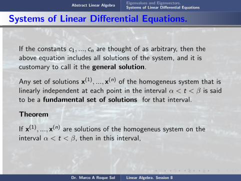
Abstract Linear AlgebraEigenvalues and Eigenvectors.Systems of Linear Differential Equations
Systems of Linear Differential Equations.
If the constants c1, ..., cn are thought of as arbitrary, then theabove equation includes all solutions of the system, and it iscustomary to call it the general solution.
Any set of solutions x(1), ..., x(n) of the homogeneus system that islinearly independent at each point in the interval α < t < β is saidto be a fundamental set of solutions for that interval.
Theorem
If x(1), ..., x(n) are solutions of the homogeneus system on theinterval α < t < β, then in this interval,
the WronskianW [x(1), ..., x(n)], given by
Dr. Marco A Roque Sol Linear Algebra. Session 8

Abstract Linear AlgebraEigenvalues and Eigenvectors.Systems of Linear Differential Equations
Systems of Linear Differential Equations.
If the constants c1, ..., cn are thought of as arbitrary, then theabove equation includes all solutions of the system, and it iscustomary to call it the general solution.
Any set of solutions x(1), ..., x(n) of the homogeneus system that islinearly independent at each point in the interval α < t < β is saidto be a fundamental set of solutions for that interval.
Theorem
If x(1), ..., x(n) are solutions of the homogeneus system on theinterval α < t < β, then in this interval, the WronskianW [x(1), ..., x(n)],
given by
Dr. Marco A Roque Sol Linear Algebra. Session 8

Abstract Linear AlgebraEigenvalues and Eigenvectors.Systems of Linear Differential Equations
Systems of Linear Differential Equations.
If the constants c1, ..., cn are thought of as arbitrary, then theabove equation includes all solutions of the system, and it iscustomary to call it the general solution.
Any set of solutions x(1), ..., x(n) of the homogeneus system that islinearly independent at each point in the interval α < t < β is saidto be a fundamental set of solutions for that interval.
Theorem
If x(1), ..., x(n) are solutions of the homogeneus system on theinterval α < t < β, then in this interval, the WronskianW [x(1), ..., x(n)], given by
Dr. Marco A Roque Sol Linear Algebra. Session 8

Abstract Linear AlgebraEigenvalues and Eigenvectors.Systems of Linear Differential Equations
Systems of Linear Differential Equations.
W [x(1), x(2) . . . x(n)] =
∣∣∣∣∣∣∣∣∣∣x(1)1 x
(2)1 . . . x
(n)1
x(1)2 x
(2)2 . . . x
(n)2
...... . . .
...
x(1)n x
(2)n . . . x
(n)n
∣∣∣∣∣∣∣∣∣∣either is identically zero or else never vanishes. To prove thistheorem is necessary to establish that
dW
dt= [p11 + p22 + ...+ pnn]W
Hence
W (t) = ce∫[p11+p22+...+pnn]dt
Dr. Marco A Roque Sol Linear Algebra. Session 8

Abstract Linear AlgebraEigenvalues and Eigenvectors.Systems of Linear Differential Equations
Systems of Linear Differential Equations.
W [x(1), x(2) . . . x(n)] =
∣∣∣∣∣∣∣∣∣∣x(1)1 x
(2)1 . . . x
(n)1
x(1)2 x
(2)2 . . . x
(n)2
...... . . .
...
x(1)n x
(2)n . . . x
(n)n
∣∣∣∣∣∣∣∣∣∣
either is identically zero or else never vanishes. To prove thistheorem is necessary to establish that
dW
dt= [p11 + p22 + ...+ pnn]W
Hence
W (t) = ce∫[p11+p22+...+pnn]dt
Dr. Marco A Roque Sol Linear Algebra. Session 8
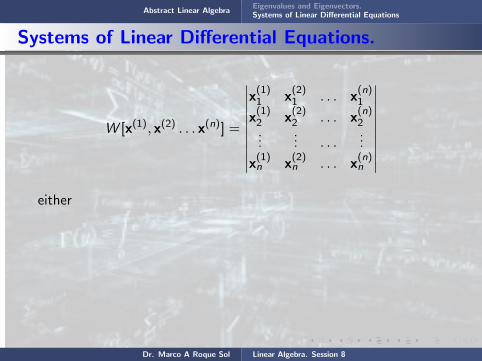
Abstract Linear AlgebraEigenvalues and Eigenvectors.Systems of Linear Differential Equations
Systems of Linear Differential Equations.
W [x(1), x(2) . . . x(n)] =
∣∣∣∣∣∣∣∣∣∣x(1)1 x
(2)1 . . . x
(n)1
x(1)2 x
(2)2 . . . x
(n)2
...... . . .
...
x(1)n x
(2)n . . . x
(n)n
∣∣∣∣∣∣∣∣∣∣either
is identically zero or else never vanishes. To prove thistheorem is necessary to establish that
dW
dt= [p11 + p22 + ...+ pnn]W
Hence
W (t) = ce∫[p11+p22+...+pnn]dt
Dr. Marco A Roque Sol Linear Algebra. Session 8

Abstract Linear AlgebraEigenvalues and Eigenvectors.Systems of Linear Differential Equations
Systems of Linear Differential Equations.
W [x(1), x(2) . . . x(n)] =
∣∣∣∣∣∣∣∣∣∣x(1)1 x
(2)1 . . . x
(n)1
x(1)2 x
(2)2 . . . x
(n)2
...... . . .
...
x(1)n x
(2)n . . . x
(n)n
∣∣∣∣∣∣∣∣∣∣either is identically zero or
else never vanishes. To prove thistheorem is necessary to establish that
dW
dt= [p11 + p22 + ...+ pnn]W
Hence
W (t) = ce∫[p11+p22+...+pnn]dt
Dr. Marco A Roque Sol Linear Algebra. Session 8
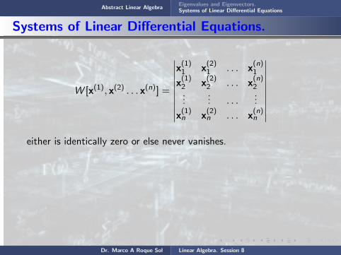
Abstract Linear AlgebraEigenvalues and Eigenvectors.Systems of Linear Differential Equations
Systems of Linear Differential Equations.
W [x(1), x(2) . . . x(n)] =
∣∣∣∣∣∣∣∣∣∣x(1)1 x
(2)1 . . . x
(n)1
x(1)2 x
(2)2 . . . x
(n)2
...... . . .
...
x(1)n x
(2)n . . . x
(n)n
∣∣∣∣∣∣∣∣∣∣either is identically zero or else never vanishes.
To prove thistheorem is necessary to establish that
dW
dt= [p11 + p22 + ...+ pnn]W
Hence
W (t) = ce∫[p11+p22+...+pnn]dt
Dr. Marco A Roque Sol Linear Algebra. Session 8

Abstract Linear AlgebraEigenvalues and Eigenvectors.Systems of Linear Differential Equations
Systems of Linear Differential Equations.
W [x(1), x(2) . . . x(n)] =
∣∣∣∣∣∣∣∣∣∣x(1)1 x
(2)1 . . . x
(n)1
x(1)2 x
(2)2 . . . x
(n)2
...... . . .
...
x(1)n x
(2)n . . . x
(n)n
∣∣∣∣∣∣∣∣∣∣either is identically zero or else never vanishes. To prove
thistheorem is necessary to establish that
dW
dt= [p11 + p22 + ...+ pnn]W
Hence
W (t) = ce∫[p11+p22+...+pnn]dt
Dr. Marco A Roque Sol Linear Algebra. Session 8

Abstract Linear AlgebraEigenvalues and Eigenvectors.Systems of Linear Differential Equations
Systems of Linear Differential Equations.
W [x(1), x(2) . . . x(n)] =
∣∣∣∣∣∣∣∣∣∣x(1)1 x
(2)1 . . . x
(n)1
x(1)2 x
(2)2 . . . x
(n)2
...... . . .
...
x(1)n x
(2)n . . . x
(n)n
∣∣∣∣∣∣∣∣∣∣either is identically zero or else never vanishes. To prove thistheorem
is necessary to establish that
dW
dt= [p11 + p22 + ...+ pnn]W
Hence
W (t) = ce∫[p11+p22+...+pnn]dt
Dr. Marco A Roque Sol Linear Algebra. Session 8
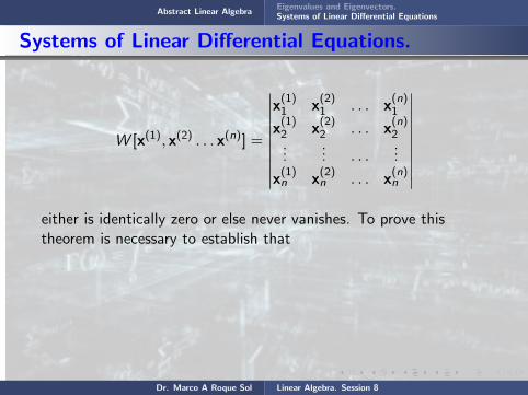
Abstract Linear AlgebraEigenvalues and Eigenvectors.Systems of Linear Differential Equations
Systems of Linear Differential Equations.
W [x(1), x(2) . . . x(n)] =
∣∣∣∣∣∣∣∣∣∣x(1)1 x
(2)1 . . . x
(n)1
x(1)2 x
(2)2 . . . x
(n)2
...... . . .
...
x(1)n x
(2)n . . . x
(n)n
∣∣∣∣∣∣∣∣∣∣either is identically zero or else never vanishes. To prove thistheorem is necessary to establish that
dW
dt= [p11 + p22 + ...+ pnn]W
Hence
W (t) = ce∫[p11+p22+...+pnn]dt
Dr. Marco A Roque Sol Linear Algebra. Session 8

Abstract Linear AlgebraEigenvalues and Eigenvectors.Systems of Linear Differential Equations
Systems of Linear Differential Equations.
W [x(1), x(2) . . . x(n)] =
∣∣∣∣∣∣∣∣∣∣x(1)1 x
(2)1 . . . x
(n)1
x(1)2 x
(2)2 . . . x
(n)2
...... . . .
...
x(1)n x
(2)n . . . x
(n)n
∣∣∣∣∣∣∣∣∣∣either is identically zero or else never vanishes. To prove thistheorem is necessary to establish that
dW
dt= [p11 + p22 + ...+ pnn]W
Hence
W (t) = ce∫[p11+p22+...+pnn]dt
Dr. Marco A Roque Sol Linear Algebra. Session 8
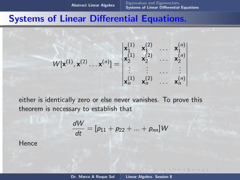
Abstract Linear AlgebraEigenvalues and Eigenvectors.Systems of Linear Differential Equations
Systems of Linear Differential Equations.
W [x(1), x(2) . . . x(n)] =
∣∣∣∣∣∣∣∣∣∣x(1)1 x
(2)1 . . . x
(n)1
x(1)2 x
(2)2 . . . x
(n)2
...... . . .
...
x(1)n x
(2)n . . . x
(n)n
∣∣∣∣∣∣∣∣∣∣either is identically zero or else never vanishes. To prove thistheorem is necessary to establish that
dW
dt= [p11 + p22 + ...+ pnn]W
Hence
W (t) = ce∫[p11+p22+...+pnn]dt
Dr. Marco A Roque Sol Linear Algebra. Session 8
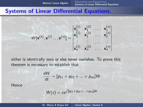
Abstract Linear AlgebraEigenvalues and Eigenvectors.Systems of Linear Differential Equations
Systems of Linear Differential Equations.
W [x(1), x(2) . . . x(n)] =
∣∣∣∣∣∣∣∣∣∣x(1)1 x
(2)1 . . . x
(n)1
x(1)2 x
(2)2 . . . x
(n)2
...... . . .
...
x(1)n x
(2)n . . . x
(n)n
∣∣∣∣∣∣∣∣∣∣either is identically zero or else never vanishes. To prove thistheorem is necessary to establish that
dW
dt= [p11 + p22 + ...+ pnn]W
Hence
W (t) = ce∫[p11+p22+...+pnn]dt
Dr. Marco A Roque Sol Linear Algebra. Session 8

Abstract Linear AlgebraEigenvalues and Eigenvectors.Systems of Linear Differential Equations
Systems of Linear Differential Equations.
Theorem
Let x(1), ..., x(n) be the solutions of the homogeneus system thatsatisfy the initial conditions x(1)(t0) = e(1), x(1)(t0) = e(2),..., x(n)(t0) = e(n), respectively, where t0 is any point in α < t < βand
e(1) =
10...0
e(2) =
01...0
· · · e(n) =
00...1
Dr. Marco A Roque Sol Linear Algebra. Session 8
Abstract Linear AlgebraEigenvalues and Eigenvectors.Systems of Linear Differential Equations
Systems of Linear Differential Equations.
Theorem
Let
x(1), ..., x(n) be the solutions of the homogeneus system thatsatisfy the initial conditions x(1)(t0) = e(1), x(1)(t0) = e(2),..., x(n)(t0) = e(n), respectively, where t0 is any point in α < t < βand
e(1) =
10...0
e(2) =
01...0
· · · e(n) =
00...1
Dr. Marco A Roque Sol Linear Algebra. Session 8

Abstract Linear AlgebraEigenvalues and Eigenvectors.Systems of Linear Differential Equations
Systems of Linear Differential Equations.
Theorem
Let x(1), ..., x(n)
be the solutions of the homogeneus system thatsatisfy the initial conditions x(1)(t0) = e(1), x(1)(t0) = e(2),..., x(n)(t0) = e(n), respectively, where t0 is any point in α < t < βand
e(1) =
10...0
e(2) =
01...0
· · · e(n) =
00...1
Dr. Marco A Roque Sol Linear Algebra. Session 8

Abstract Linear AlgebraEigenvalues and Eigenvectors.Systems of Linear Differential Equations
Systems of Linear Differential Equations.
Theorem
Let x(1), ..., x(n) be the solutions
of the homogeneus system thatsatisfy the initial conditions x(1)(t0) = e(1), x(1)(t0) = e(2),..., x(n)(t0) = e(n), respectively, where t0 is any point in α < t < βand
e(1) =
10...0
e(2) =
01...0
· · · e(n) =
00...1
Dr. Marco A Roque Sol Linear Algebra. Session 8

Abstract Linear AlgebraEigenvalues and Eigenvectors.Systems of Linear Differential Equations
Systems of Linear Differential Equations.
Theorem
Let x(1), ..., x(n) be the solutions of the homogeneus system
thatsatisfy the initial conditions x(1)(t0) = e(1), x(1)(t0) = e(2),..., x(n)(t0) = e(n), respectively, where t0 is any point in α < t < βand
e(1) =
10...0
e(2) =
01...0
· · · e(n) =
00...1
Dr. Marco A Roque Sol Linear Algebra. Session 8

Abstract Linear AlgebraEigenvalues and Eigenvectors.Systems of Linear Differential Equations
Systems of Linear Differential Equations.
Theorem
Let x(1), ..., x(n) be the solutions of the homogeneus system thatsatisfy
the initial conditions x(1)(t0) = e(1), x(1)(t0) = e(2),..., x(n)(t0) = e(n), respectively, where t0 is any point in α < t < βand
e(1) =
10...0
e(2) =
01...0
· · · e(n) =
00...1
Dr. Marco A Roque Sol Linear Algebra. Session 8

Abstract Linear AlgebraEigenvalues and Eigenvectors.Systems of Linear Differential Equations
Systems of Linear Differential Equations.
Theorem
Let x(1), ..., x(n) be the solutions of the homogeneus system thatsatisfy the initial conditions
x(1)(t0) = e(1), x(1)(t0) = e(2),..., x(n)(t0) = e(n), respectively, where t0 is any point in α < t < βand
e(1) =
10...0
e(2) =
01...0
· · · e(n) =
00...1
Dr. Marco A Roque Sol Linear Algebra. Session 8

Abstract Linear AlgebraEigenvalues and Eigenvectors.Systems of Linear Differential Equations
Systems of Linear Differential Equations.
Theorem
Let x(1), ..., x(n) be the solutions of the homogeneus system thatsatisfy the initial conditions x(1)(t0) = e(1),
x(1)(t0) = e(2),..., x(n)(t0) = e(n), respectively, where t0 is any point in α < t < βand
e(1) =
10...0
e(2) =
01...0
· · · e(n) =
00...1
Dr. Marco A Roque Sol Linear Algebra. Session 8

Abstract Linear AlgebraEigenvalues and Eigenvectors.Systems of Linear Differential Equations
Systems of Linear Differential Equations.
Theorem
Let x(1), ..., x(n) be the solutions of the homogeneus system thatsatisfy the initial conditions x(1)(t0) = e(1), x(1)(t0) = e(2),...,
x(n)(t0) = e(n), respectively, where t0 is any point in α < t < βand
e(1) =
10...0
e(2) =
01...0
· · · e(n) =
00...1
Dr. Marco A Roque Sol Linear Algebra. Session 8

Abstract Linear AlgebraEigenvalues and Eigenvectors.Systems of Linear Differential Equations
Systems of Linear Differential Equations.
Theorem
Let x(1), ..., x(n) be the solutions of the homogeneus system thatsatisfy the initial conditions x(1)(t0) = e(1), x(1)(t0) = e(2),..., x(n)(t0) = e(n), respectively,
where t0 is any point in α < t < βand
e(1) =
10...0
e(2) =
01...0
· · · e(n) =
00...1
Dr. Marco A Roque Sol Linear Algebra. Session 8

Abstract Linear AlgebraEigenvalues and Eigenvectors.Systems of Linear Differential Equations
Systems of Linear Differential Equations.
Theorem
Let x(1), ..., x(n) be the solutions of the homogeneus system thatsatisfy the initial conditions x(1)(t0) = e(1), x(1)(t0) = e(2),..., x(n)(t0) = e(n), respectively, where t0
is any point in α < t < βand
e(1) =
10...0
e(2) =
01...0
· · · e(n) =
00...1
Dr. Marco A Roque Sol Linear Algebra. Session 8

Abstract Linear AlgebraEigenvalues and Eigenvectors.Systems of Linear Differential Equations
Systems of Linear Differential Equations.
Theorem
Let x(1), ..., x(n) be the solutions of the homogeneus system thatsatisfy the initial conditions x(1)(t0) = e(1), x(1)(t0) = e(2),..., x(n)(t0) = e(n), respectively, where t0 is any point in
α < t < βand
e(1) =
10...0
e(2) =
01...0
· · · e(n) =
00...1
Dr. Marco A Roque Sol Linear Algebra. Session 8

Abstract Linear AlgebraEigenvalues and Eigenvectors.Systems of Linear Differential Equations
Systems of Linear Differential Equations.
Theorem
Let x(1), ..., x(n) be the solutions of the homogeneus system thatsatisfy the initial conditions x(1)(t0) = e(1), x(1)(t0) = e(2),..., x(n)(t0) = e(n), respectively, where t0 is any point in α < t < βand
e(1) =
10...0
e(2) =
01...0
· · · e(n) =
00...1
Dr. Marco A Roque Sol Linear Algebra. Session 8

Abstract Linear AlgebraEigenvalues and Eigenvectors.Systems of Linear Differential Equations
Systems of Linear Differential Equations.
Theorem
Let x(1), ..., x(n) be the solutions of the homogeneus system thatsatisfy the initial conditions x(1)(t0) = e(1), x(1)(t0) = e(2),..., x(n)(t0) = e(n), respectively, where t0 is any point in α < t < βand
e(1) =
10...0
e(2) =
01...0
· · ·
e(n) =
00...1
Dr. Marco A Roque Sol Linear Algebra. Session 8
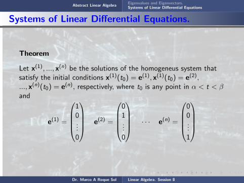
Abstract Linear AlgebraEigenvalues and Eigenvectors.Systems of Linear Differential Equations
Systems of Linear Differential Equations.
Theorem
Let x(1), ..., x(n) be the solutions of the homogeneus system thatsatisfy the initial conditions x(1)(t0) = e(1), x(1)(t0) = e(2),..., x(n)(t0) = e(n), respectively, where t0 is any point in α < t < βand
e(1) =
10...0
e(2) =
01...0
· · · e(n) =
00...1
Dr. Marco A Roque Sol Linear Algebra. Session 8

Abstract Linear AlgebraEigenvalues and Eigenvectors.Systems of Linear Differential Equations
Systems of Linear Differential Equations.
Then, x(1), ..., x(n) form a fundamental set of solutions of thehomogeneous system.
Finally in the case that the solution is complex-valued, we have thefollowing result.
Theorem
Consider the homogeneous system
X′ = P(t)X
where each element of P is a real-valued continuous function. Ifx = u(t) + i v(t) is a complex-valued solution, then its real partu(t) and its imaginary part v(t) are also solutions of this equation.
Dr. Marco A Roque Sol Linear Algebra. Session 8

Abstract Linear AlgebraEigenvalues and Eigenvectors.Systems of Linear Differential Equations
Systems of Linear Differential Equations.
Then,
x(1), ..., x(n) form a fundamental set of solutions of thehomogeneous system.
Finally in the case that the solution is complex-valued, we have thefollowing result.
Theorem
Consider the homogeneous system
X′ = P(t)X
where each element of P is a real-valued continuous function. Ifx = u(t) + i v(t) is a complex-valued solution, then its real partu(t) and its imaginary part v(t) are also solutions of this equation.
Dr. Marco A Roque Sol Linear Algebra. Session 8
Abstract Linear AlgebraEigenvalues and Eigenvectors.Systems of Linear Differential Equations
Systems of Linear Differential Equations.
Then, x(1), ..., x(n)
form a fundamental set of solutions of thehomogeneous system.
Finally in the case that the solution is complex-valued, we have thefollowing result.
Theorem
Consider the homogeneous system
X′ = P(t)X
where each element of P is a real-valued continuous function. Ifx = u(t) + i v(t) is a complex-valued solution, then its real partu(t) and its imaginary part v(t) are also solutions of this equation.
Dr. Marco A Roque Sol Linear Algebra. Session 8

Abstract Linear AlgebraEigenvalues and Eigenvectors.Systems of Linear Differential Equations
Systems of Linear Differential Equations.
Then, x(1), ..., x(n) form a fundamental set
of solutions of thehomogeneous system.
Finally in the case that the solution is complex-valued, we have thefollowing result.
Theorem
Consider the homogeneous system
X′ = P(t)X
where each element of P is a real-valued continuous function. Ifx = u(t) + i v(t) is a complex-valued solution, then its real partu(t) and its imaginary part v(t) are also solutions of this equation.
Dr. Marco A Roque Sol Linear Algebra. Session 8

Abstract Linear AlgebraEigenvalues and Eigenvectors.Systems of Linear Differential Equations
Systems of Linear Differential Equations.
Then, x(1), ..., x(n) form a fundamental set of solutions
of thehomogeneous system.
Finally in the case that the solution is complex-valued, we have thefollowing result.
Theorem
Consider the homogeneous system
X′ = P(t)X
where each element of P is a real-valued continuous function. Ifx = u(t) + i v(t) is a complex-valued solution, then its real partu(t) and its imaginary part v(t) are also solutions of this equation.
Dr. Marco A Roque Sol Linear Algebra. Session 8

Abstract Linear AlgebraEigenvalues and Eigenvectors.Systems of Linear Differential Equations
Systems of Linear Differential Equations.
Then, x(1), ..., x(n) form a fundamental set of solutions of thehomogeneous system.
Finally in the case that the solution is complex-valued, we have thefollowing result.
Theorem
Consider the homogeneous system
X′ = P(t)X
where each element of P is a real-valued continuous function. Ifx = u(t) + i v(t) is a complex-valued solution, then its real partu(t) and its imaginary part v(t) are also solutions of this equation.
Dr. Marco A Roque Sol Linear Algebra. Session 8
Abstract Linear AlgebraEigenvalues and Eigenvectors.Systems of Linear Differential Equations
Systems of Linear Differential Equations.
Then, x(1), ..., x(n) form a fundamental set of solutions of thehomogeneous system.
Finally
in the case that the solution is complex-valued, we have thefollowing result.
Theorem
Consider the homogeneous system
X′ = P(t)X
where each element of P is a real-valued continuous function. Ifx = u(t) + i v(t) is a complex-valued solution, then its real partu(t) and its imaginary part v(t) are also solutions of this equation.
Dr. Marco A Roque Sol Linear Algebra. Session 8

Abstract Linear AlgebraEigenvalues and Eigenvectors.Systems of Linear Differential Equations
Systems of Linear Differential Equations.
Then, x(1), ..., x(n) form a fundamental set of solutions of thehomogeneous system.
Finally in the case
that the solution is complex-valued, we have thefollowing result.
Theorem
Consider the homogeneous system
X′ = P(t)X
where each element of P is a real-valued continuous function. Ifx = u(t) + i v(t) is a complex-valued solution, then its real partu(t) and its imaginary part v(t) are also solutions of this equation.
Dr. Marco A Roque Sol Linear Algebra. Session 8
Abstract Linear AlgebraEigenvalues and Eigenvectors.Systems of Linear Differential Equations
Systems of Linear Differential Equations.
Then, x(1), ..., x(n) form a fundamental set of solutions of thehomogeneous system.
Finally in the case that the solution
is complex-valued, we have thefollowing result.
Theorem
Consider the homogeneous system
X′ = P(t)X
where each element of P is a real-valued continuous function. Ifx = u(t) + i v(t) is a complex-valued solution, then its real partu(t) and its imaginary part v(t) are also solutions of this equation.
Dr. Marco A Roque Sol Linear Algebra. Session 8
Abstract Linear AlgebraEigenvalues and Eigenvectors.Systems of Linear Differential Equations
Systems of Linear Differential Equations.
Then, x(1), ..., x(n) form a fundamental set of solutions of thehomogeneous system.
Finally in the case that the solution is complex-valued,
we have thefollowing result.
Theorem
Consider the homogeneous system
X′ = P(t)X
where each element of P is a real-valued continuous function. Ifx = u(t) + i v(t) is a complex-valued solution, then its real partu(t) and its imaginary part v(t) are also solutions of this equation.
Dr. Marco A Roque Sol Linear Algebra. Session 8

Abstract Linear AlgebraEigenvalues and Eigenvectors.Systems of Linear Differential Equations
Systems of Linear Differential Equations.
Then, x(1), ..., x(n) form a fundamental set of solutions of thehomogeneous system.
Finally in the case that the solution is complex-valued, we have
thefollowing result.
Theorem
Consider the homogeneous system
X′ = P(t)X
where each element of P is a real-valued continuous function. Ifx = u(t) + i v(t) is a complex-valued solution, then its real partu(t) and its imaginary part v(t) are also solutions of this equation.
Dr. Marco A Roque Sol Linear Algebra. Session 8
Abstract Linear AlgebraEigenvalues and Eigenvectors.Systems of Linear Differential Equations
Systems of Linear Differential Equations.
Then, x(1), ..., x(n) form a fundamental set of solutions of thehomogeneous system.
Finally in the case that the solution is complex-valued, we have thefollowing result.
Theorem
Consider the homogeneous system
X′ = P(t)X
where each element of P is a real-valued continuous function. Ifx = u(t) + i v(t) is a complex-valued solution, then its real partu(t) and its imaginary part v(t) are also solutions of this equation.
Dr. Marco A Roque Sol Linear Algebra. Session 8

Abstract Linear AlgebraEigenvalues and Eigenvectors.Systems of Linear Differential Equations
Systems of Linear Differential Equations.
Then, x(1), ..., x(n) form a fundamental set of solutions of thehomogeneous system.
Finally in the case that the solution is complex-valued, we have thefollowing result.
Theorem
Consider
the homogeneous system
X′ = P(t)X
where each element of P is a real-valued continuous function. Ifx = u(t) + i v(t) is a complex-valued solution, then its real partu(t) and its imaginary part v(t) are also solutions of this equation.
Dr. Marco A Roque Sol Linear Algebra. Session 8

Abstract Linear AlgebraEigenvalues and Eigenvectors.Systems of Linear Differential Equations
Systems of Linear Differential Equations.
Then, x(1), ..., x(n) form a fundamental set of solutions of thehomogeneous system.
Finally in the case that the solution is complex-valued, we have thefollowing result.
Theorem
Consider the homogeneous system
X′ = P(t)X
where each element of P is a real-valued continuous function. Ifx = u(t) + i v(t) is a complex-valued solution, then its real partu(t) and its imaginary part v(t) are also solutions of this equation.
Dr. Marco A Roque Sol Linear Algebra. Session 8
Abstract Linear AlgebraEigenvalues and Eigenvectors.Systems of Linear Differential Equations
Systems of Linear Differential Equations.
Then, x(1), ..., x(n) form a fundamental set of solutions of thehomogeneous system.
Finally in the case that the solution is complex-valued, we have thefollowing result.
Theorem
Consider the homogeneous system
X′ = P(t)X
where each element
of P is a real-valued continuous function. Ifx = u(t) + i v(t) is a complex-valued solution, then its real partu(t) and its imaginary part v(t) are also solutions of this equation.
Dr. Marco A Roque Sol Linear Algebra. Session 8

Abstract Linear AlgebraEigenvalues and Eigenvectors.Systems of Linear Differential Equations
Systems of Linear Differential Equations.
Then, x(1), ..., x(n) form a fundamental set of solutions of thehomogeneous system.
Finally in the case that the solution is complex-valued, we have thefollowing result.
Theorem
Consider the homogeneous system
X′ = P(t)X
where each element of P
is a real-valued continuous function. Ifx = u(t) + i v(t) is a complex-valued solution, then its real partu(t) and its imaginary part v(t) are also solutions of this equation.
Dr. Marco A Roque Sol Linear Algebra. Session 8
Abstract Linear AlgebraEigenvalues and Eigenvectors.Systems of Linear Differential Equations
Systems of Linear Differential Equations.
Then, x(1), ..., x(n) form a fundamental set of solutions of thehomogeneous system.
Finally in the case that the solution is complex-valued, we have thefollowing result.
Theorem
Consider the homogeneous system
X′ = P(t)X
where each element of P is a real-valued
continuous function. Ifx = u(t) + i v(t) is a complex-valued solution, then its real partu(t) and its imaginary part v(t) are also solutions of this equation.
Dr. Marco A Roque Sol Linear Algebra. Session 8
Abstract Linear AlgebraEigenvalues and Eigenvectors.Systems of Linear Differential Equations
Systems of Linear Differential Equations.
Then, x(1), ..., x(n) form a fundamental set of solutions of thehomogeneous system.
Finally in the case that the solution is complex-valued, we have thefollowing result.
Theorem
Consider the homogeneous system
X′ = P(t)X
where each element of P is a real-valued continuous function.
Ifx = u(t) + i v(t) is a complex-valued solution, then its real partu(t) and its imaginary part v(t) are also solutions of this equation.
Dr. Marco A Roque Sol Linear Algebra. Session 8

Abstract Linear AlgebraEigenvalues and Eigenvectors.Systems of Linear Differential Equations
Systems of Linear Differential Equations.
Then, x(1), ..., x(n) form a fundamental set of solutions of thehomogeneous system.
Finally in the case that the solution is complex-valued, we have thefollowing result.
Theorem
Consider the homogeneous system
X′ = P(t)X
where each element of P is a real-valued continuous function. Ifx = u(t) + i v(t)
is a complex-valued solution, then its real partu(t) and its imaginary part v(t) are also solutions of this equation.
Dr. Marco A Roque Sol Linear Algebra. Session 8

Abstract Linear AlgebraEigenvalues and Eigenvectors.Systems of Linear Differential Equations
Systems of Linear Differential Equations.
Then, x(1), ..., x(n) form a fundamental set of solutions of thehomogeneous system.
Finally in the case that the solution is complex-valued, we have thefollowing result.
Theorem
Consider the homogeneous system
X′ = P(t)X
where each element of P is a real-valued continuous function. Ifx = u(t) + i v(t) is a complex-valued solution,
then its real partu(t) and its imaginary part v(t) are also solutions of this equation.
Dr. Marco A Roque Sol Linear Algebra. Session 8

Abstract Linear AlgebraEigenvalues and Eigenvectors.Systems of Linear Differential Equations
Systems of Linear Differential Equations.
Then, x(1), ..., x(n) form a fundamental set of solutions of thehomogeneous system.
Finally in the case that the solution is complex-valued, we have thefollowing result.
Theorem
Consider the homogeneous system
X′ = P(t)X
where each element of P is a real-valued continuous function. Ifx = u(t) + i v(t) is a complex-valued solution, then its real part
u(t) and its imaginary part v(t) are also solutions of this equation.
Dr. Marco A Roque Sol Linear Algebra. Session 8

Abstract Linear AlgebraEigenvalues and Eigenvectors.Systems of Linear Differential Equations
Systems of Linear Differential Equations.
Then, x(1), ..., x(n) form a fundamental set of solutions of thehomogeneous system.
Finally in the case that the solution is complex-valued, we have thefollowing result.
Theorem
Consider the homogeneous system
X′ = P(t)X
where each element of P is a real-valued continuous function. Ifx = u(t) + i v(t) is a complex-valued solution, then its real partu(t) and
its imaginary part v(t) are also solutions of this equation.
Dr. Marco A Roque Sol Linear Algebra. Session 8

Abstract Linear AlgebraEigenvalues and Eigenvectors.Systems of Linear Differential Equations
Systems of Linear Differential Equations.
Then, x(1), ..., x(n) form a fundamental set of solutions of thehomogeneous system.
Finally in the case that the solution is complex-valued, we have thefollowing result.
Theorem
Consider the homogeneous system
X′ = P(t)X
where each element of P is a real-valued continuous function. Ifx = u(t) + i v(t) is a complex-valued solution, then its real partu(t) and its imaginary part
v(t) are also solutions of this equation.
Dr. Marco A Roque Sol Linear Algebra. Session 8

Abstract Linear AlgebraEigenvalues and Eigenvectors.Systems of Linear Differential Equations
Systems of Linear Differential Equations.
Then, x(1), ..., x(n) form a fundamental set of solutions of thehomogeneous system.
Finally in the case that the solution is complex-valued, we have thefollowing result.
Theorem
Consider the homogeneous system
X′ = P(t)X
where each element of P is a real-valued continuous function. Ifx = u(t) + i v(t) is a complex-valued solution, then its real partu(t) and its imaginary part v(t)
are also solutions of this equation.
Dr. Marco A Roque Sol Linear Algebra. Session 8
Abstract Linear AlgebraEigenvalues and Eigenvectors.Systems of Linear Differential Equations
Systems of Linear Differential Equations.
Then, x(1), ..., x(n) form a fundamental set of solutions of thehomogeneous system.
Finally in the case that the solution is complex-valued, we have thefollowing result.
Theorem
Consider the homogeneous system
X′ = P(t)X
where each element of P is a real-valued continuous function. Ifx = u(t) + i v(t) is a complex-valued solution, then its real partu(t) and its imaginary part v(t) are also solutions
of this equation.
Dr. Marco A Roque Sol Linear Algebra. Session 8

Abstract Linear AlgebraEigenvalues and Eigenvectors.Systems of Linear Differential Equations
Systems of Linear Differential Equations.
Then, x(1), ..., x(n) form a fundamental set of solutions of thehomogeneous system.
Finally in the case that the solution is complex-valued, we have thefollowing result.
Theorem
Consider the homogeneous system
X′ = P(t)X
where each element of P is a real-valued continuous function. Ifx = u(t) + i v(t) is a complex-valued solution, then its real partu(t) and its imaginary part v(t) are also solutions of this equation.
Dr. Marco A Roque Sol Linear Algebra. Session 8

Abstract Linear AlgebraEigenvalues and Eigenvectors.Systems of Linear Differential Equations
Systems of Linear Differential Equations.
We will concentrate most of our attention on systems ofhomogeneous linear differential equations with constant coefficients
x′ = Ax
where A is a constant n × n matrix. Unless stated otherwise, wewill assume further that all the elements of A are real (rather thancomplex) numbers.
The case n = 2 is particularly important and lends itself tovisualization in the x1x2 − plane, called the phase plane. Byevaluating Ax at a large number of points and plotting theresulting vectors, we obtain a direction field of tangent vectors tosolutions of the system of differential equations.
Dr. Marco A Roque Sol Linear Algebra. Session 8
Abstract Linear AlgebraEigenvalues and Eigenvectors.Systems of Linear Differential Equations
Systems of Linear Differential Equations.
We will concentrate
most of our attention on systems ofhomogeneous linear differential equations with constant coefficients
x′ = Ax
where A is a constant n × n matrix. Unless stated otherwise, wewill assume further that all the elements of A are real (rather thancomplex) numbers.
The case n = 2 is particularly important and lends itself tovisualization in the x1x2 − plane, called the phase plane. Byevaluating Ax at a large number of points and plotting theresulting vectors, we obtain a direction field of tangent vectors tosolutions of the system of differential equations.
Dr. Marco A Roque Sol Linear Algebra. Session 8

Abstract Linear AlgebraEigenvalues and Eigenvectors.Systems of Linear Differential Equations
Systems of Linear Differential Equations.
We will concentrate most of our attention
on systems ofhomogeneous linear differential equations with constant coefficients
x′ = Ax
where A is a constant n × n matrix. Unless stated otherwise, wewill assume further that all the elements of A are real (rather thancomplex) numbers.
The case n = 2 is particularly important and lends itself tovisualization in the x1x2 − plane, called the phase plane. Byevaluating Ax at a large number of points and plotting theresulting vectors, we obtain a direction field of tangent vectors tosolutions of the system of differential equations.
Dr. Marco A Roque Sol Linear Algebra. Session 8

Abstract Linear AlgebraEigenvalues and Eigenvectors.Systems of Linear Differential Equations
Systems of Linear Differential Equations.
We will concentrate most of our attention on systems of
homogeneous linear differential equations with constant coefficients
x′ = Ax
where A is a constant n × n matrix. Unless stated otherwise, wewill assume further that all the elements of A are real (rather thancomplex) numbers.
The case n = 2 is particularly important and lends itself tovisualization in the x1x2 − plane, called the phase plane. Byevaluating Ax at a large number of points and plotting theresulting vectors, we obtain a direction field of tangent vectors tosolutions of the system of differential equations.
Dr. Marco A Roque Sol Linear Algebra. Session 8

Abstract Linear AlgebraEigenvalues and Eigenvectors.Systems of Linear Differential Equations
Systems of Linear Differential Equations.
We will concentrate most of our attention on systems ofhomogeneous linear
differential equations with constant coefficients
x′ = Ax
where A is a constant n × n matrix. Unless stated otherwise, wewill assume further that all the elements of A are real (rather thancomplex) numbers.
The case n = 2 is particularly important and lends itself tovisualization in the x1x2 − plane, called the phase plane. Byevaluating Ax at a large number of points and plotting theresulting vectors, we obtain a direction field of tangent vectors tosolutions of the system of differential equations.
Dr. Marco A Roque Sol Linear Algebra. Session 8

Abstract Linear AlgebraEigenvalues and Eigenvectors.Systems of Linear Differential Equations
Systems of Linear Differential Equations.
We will concentrate most of our attention on systems ofhomogeneous linear differential equations
with constant coefficients
x′ = Ax
where A is a constant n × n matrix. Unless stated otherwise, wewill assume further that all the elements of A are real (rather thancomplex) numbers.
The case n = 2 is particularly important and lends itself tovisualization in the x1x2 − plane, called the phase plane. Byevaluating Ax at a large number of points and plotting theresulting vectors, we obtain a direction field of tangent vectors tosolutions of the system of differential equations.
Dr. Marco A Roque Sol Linear Algebra. Session 8
Abstract Linear AlgebraEigenvalues and Eigenvectors.Systems of Linear Differential Equations
Systems of Linear Differential Equations.
We will concentrate most of our attention on systems ofhomogeneous linear differential equations with constant coefficients
x′ = Ax
where A is a constant n × n matrix. Unless stated otherwise, wewill assume further that all the elements of A are real (rather thancomplex) numbers.
The case n = 2 is particularly important and lends itself tovisualization in the x1x2 − plane, called the phase plane. Byevaluating Ax at a large number of points and plotting theresulting vectors, we obtain a direction field of tangent vectors tosolutions of the system of differential equations.
Dr. Marco A Roque Sol Linear Algebra. Session 8

Abstract Linear AlgebraEigenvalues and Eigenvectors.Systems of Linear Differential Equations
Systems of Linear Differential Equations.
We will concentrate most of our attention on systems ofhomogeneous linear differential equations with constant coefficients
x′ = Ax
where A
is a constant n × n matrix. Unless stated otherwise, wewill assume further that all the elements of A are real (rather thancomplex) numbers.
The case n = 2 is particularly important and lends itself tovisualization in the x1x2 − plane, called the phase plane. Byevaluating Ax at a large number of points and plotting theresulting vectors, we obtain a direction field of tangent vectors tosolutions of the system of differential equations.
Dr. Marco A Roque Sol Linear Algebra. Session 8

Abstract Linear AlgebraEigenvalues and Eigenvectors.Systems of Linear Differential Equations
Systems of Linear Differential Equations.
We will concentrate most of our attention on systems ofhomogeneous linear differential equations with constant coefficients
x′ = Ax
where A is a constant
n × n matrix. Unless stated otherwise, wewill assume further that all the elements of A are real (rather thancomplex) numbers.
The case n = 2 is particularly important and lends itself tovisualization in the x1x2 − plane, called the phase plane. Byevaluating Ax at a large number of points and plotting theresulting vectors, we obtain a direction field of tangent vectors tosolutions of the system of differential equations.
Dr. Marco A Roque Sol Linear Algebra. Session 8
Abstract Linear AlgebraEigenvalues and Eigenvectors.Systems of Linear Differential Equations
Systems of Linear Differential Equations.
We will concentrate most of our attention on systems ofhomogeneous linear differential equations with constant coefficients
x′ = Ax
where A is a constant n × n matrix.
Unless stated otherwise, wewill assume further that all the elements of A are real (rather thancomplex) numbers.
The case n = 2 is particularly important and lends itself tovisualization in the x1x2 − plane, called the phase plane. Byevaluating Ax at a large number of points and plotting theresulting vectors, we obtain a direction field of tangent vectors tosolutions of the system of differential equations.
Dr. Marco A Roque Sol Linear Algebra. Session 8

Abstract Linear AlgebraEigenvalues and Eigenvectors.Systems of Linear Differential Equations
Systems of Linear Differential Equations.
We will concentrate most of our attention on systems ofhomogeneous linear differential equations with constant coefficients
x′ = Ax
where A is a constant n × n matrix. Unless stated otherwise,
wewill assume further that all the elements of A are real (rather thancomplex) numbers.
The case n = 2 is particularly important and lends itself tovisualization in the x1x2 − plane, called the phase plane. Byevaluating Ax at a large number of points and plotting theresulting vectors, we obtain a direction field of tangent vectors tosolutions of the system of differential equations.
Dr. Marco A Roque Sol Linear Algebra. Session 8

Abstract Linear AlgebraEigenvalues and Eigenvectors.Systems of Linear Differential Equations
Systems of Linear Differential Equations.
We will concentrate most of our attention on systems ofhomogeneous linear differential equations with constant coefficients
x′ = Ax
where A is a constant n × n matrix. Unless stated otherwise, wewill assume further
that all the elements of A are real (rather thancomplex) numbers.
The case n = 2 is particularly important and lends itself tovisualization in the x1x2 − plane, called the phase plane. Byevaluating Ax at a large number of points and plotting theresulting vectors, we obtain a direction field of tangent vectors tosolutions of the system of differential equations.
Dr. Marco A Roque Sol Linear Algebra. Session 8
Abstract Linear AlgebraEigenvalues and Eigenvectors.Systems of Linear Differential Equations
Systems of Linear Differential Equations.
We will concentrate most of our attention on systems ofhomogeneous linear differential equations with constant coefficients
x′ = Ax
where A is a constant n × n matrix. Unless stated otherwise, wewill assume further that all the elements
of A are real (rather thancomplex) numbers.
The case n = 2 is particularly important and lends itself tovisualization in the x1x2 − plane, called the phase plane. Byevaluating Ax at a large number of points and plotting theresulting vectors, we obtain a direction field of tangent vectors tosolutions of the system of differential equations.
Dr. Marco A Roque Sol Linear Algebra. Session 8

Abstract Linear AlgebraEigenvalues and Eigenvectors.Systems of Linear Differential Equations
Systems of Linear Differential Equations.
We will concentrate most of our attention on systems ofhomogeneous linear differential equations with constant coefficients
x′ = Ax
where A is a constant n × n matrix. Unless stated otherwise, wewill assume further that all the elements of A
are real (rather thancomplex) numbers.
The case n = 2 is particularly important and lends itself tovisualization in the x1x2 − plane, called the phase plane. Byevaluating Ax at a large number of points and plotting theresulting vectors, we obtain a direction field of tangent vectors tosolutions of the system of differential equations.
Dr. Marco A Roque Sol Linear Algebra. Session 8

Abstract Linear AlgebraEigenvalues and Eigenvectors.Systems of Linear Differential Equations
Systems of Linear Differential Equations.
We will concentrate most of our attention on systems ofhomogeneous linear differential equations with constant coefficients
x′ = Ax
where A is a constant n × n matrix. Unless stated otherwise, wewill assume further that all the elements of A are real
(rather thancomplex) numbers.
The case n = 2 is particularly important and lends itself tovisualization in the x1x2 − plane, called the phase plane. Byevaluating Ax at a large number of points and plotting theresulting vectors, we obtain a direction field of tangent vectors tosolutions of the system of differential equations.
Dr. Marco A Roque Sol Linear Algebra. Session 8

Abstract Linear AlgebraEigenvalues and Eigenvectors.Systems of Linear Differential Equations
Systems of Linear Differential Equations.
We will concentrate most of our attention on systems ofhomogeneous linear differential equations with constant coefficients
x′ = Ax
where A is a constant n × n matrix. Unless stated otherwise, wewill assume further that all the elements of A are real (rather thancomplex)
numbers.
The case n = 2 is particularly important and lends itself tovisualization in the x1x2 − plane, called the phase plane. Byevaluating Ax at a large number of points and plotting theresulting vectors, we obtain a direction field of tangent vectors tosolutions of the system of differential equations.
Dr. Marco A Roque Sol Linear Algebra. Session 8
Abstract Linear AlgebraEigenvalues and Eigenvectors.Systems of Linear Differential Equations
Systems of Linear Differential Equations.
We will concentrate most of our attention on systems ofhomogeneous linear differential equations with constant coefficients
x′ = Ax
where A is a constant n × n matrix. Unless stated otherwise, wewill assume further that all the elements of A are real (rather thancomplex) numbers.
The case n = 2 is particularly important and lends itself tovisualization in the x1x2 − plane, called the phase plane. Byevaluating Ax at a large number of points and plotting theresulting vectors, we obtain a direction field of tangent vectors tosolutions of the system of differential equations.
Dr. Marco A Roque Sol Linear Algebra. Session 8

Abstract Linear AlgebraEigenvalues and Eigenvectors.Systems of Linear Differential Equations
Systems of Linear Differential Equations.
We will concentrate most of our attention on systems ofhomogeneous linear differential equations with constant coefficients
x′ = Ax
where A is a constant n × n matrix. Unless stated otherwise, wewill assume further that all the elements of A are real (rather thancomplex) numbers.
The case
n = 2 is particularly important and lends itself tovisualization in the x1x2 − plane, called the phase plane. Byevaluating Ax at a large number of points and plotting theresulting vectors, we obtain a direction field of tangent vectors tosolutions of the system of differential equations.
Dr. Marco A Roque Sol Linear Algebra. Session 8

Abstract Linear AlgebraEigenvalues and Eigenvectors.Systems of Linear Differential Equations
Systems of Linear Differential Equations.
We will concentrate most of our attention on systems ofhomogeneous linear differential equations with constant coefficients
x′ = Ax
where A is a constant n × n matrix. Unless stated otherwise, wewill assume further that all the elements of A are real (rather thancomplex) numbers.
The case n = 2
is particularly important and lends itself tovisualization in the x1x2 − plane, called the phase plane. Byevaluating Ax at a large number of points and plotting theresulting vectors, we obtain a direction field of tangent vectors tosolutions of the system of differential equations.
Dr. Marco A Roque Sol Linear Algebra. Session 8

Abstract Linear AlgebraEigenvalues and Eigenvectors.Systems of Linear Differential Equations
Systems of Linear Differential Equations.
We will concentrate most of our attention on systems ofhomogeneous linear differential equations with constant coefficients
x′ = Ax
where A is a constant n × n matrix. Unless stated otherwise, wewill assume further that all the elements of A are real (rather thancomplex) numbers.
The case n = 2 is particularly important and
lends itself tovisualization in the x1x2 − plane, called the phase plane. Byevaluating Ax at a large number of points and plotting theresulting vectors, we obtain a direction field of tangent vectors tosolutions of the system of differential equations.
Dr. Marco A Roque Sol Linear Algebra. Session 8
Abstract Linear AlgebraEigenvalues and Eigenvectors.Systems of Linear Differential Equations
Systems of Linear Differential Equations.
We will concentrate most of our attention on systems ofhomogeneous linear differential equations with constant coefficients
x′ = Ax
where A is a constant n × n matrix. Unless stated otherwise, wewill assume further that all the elements of A are real (rather thancomplex) numbers.
The case n = 2 is particularly important and lends itself
tovisualization in the x1x2 − plane, called the phase plane. Byevaluating Ax at a large number of points and plotting theresulting vectors, we obtain a direction field of tangent vectors tosolutions of the system of differential equations.
Dr. Marco A Roque Sol Linear Algebra. Session 8
Abstract Linear AlgebraEigenvalues and Eigenvectors.Systems of Linear Differential Equations
Systems of Linear Differential Equations.
We will concentrate most of our attention on systems ofhomogeneous linear differential equations with constant coefficients
x′ = Ax
where A is a constant n × n matrix. Unless stated otherwise, wewill assume further that all the elements of A are real (rather thancomplex) numbers.
The case n = 2 is particularly important and lends itself tovisualization
in the x1x2 − plane, called the phase plane. Byevaluating Ax at a large number of points and plotting theresulting vectors, we obtain a direction field of tangent vectors tosolutions of the system of differential equations.
Dr. Marco A Roque Sol Linear Algebra. Session 8
Abstract Linear AlgebraEigenvalues and Eigenvectors.Systems of Linear Differential Equations
Systems of Linear Differential Equations.
We will concentrate most of our attention on systems ofhomogeneous linear differential equations with constant coefficients
x′ = Ax
where A is a constant n × n matrix. Unless stated otherwise, wewill assume further that all the elements of A are real (rather thancomplex) numbers.
The case n = 2 is particularly important and lends itself tovisualization in the x1x2 − plane,
called the phase plane. Byevaluating Ax at a large number of points and plotting theresulting vectors, we obtain a direction field of tangent vectors tosolutions of the system of differential equations.
Dr. Marco A Roque Sol Linear Algebra. Session 8

Abstract Linear AlgebraEigenvalues and Eigenvectors.Systems of Linear Differential Equations
Systems of Linear Differential Equations.
We will concentrate most of our attention on systems ofhomogeneous linear differential equations with constant coefficients
x′ = Ax
where A is a constant n × n matrix. Unless stated otherwise, wewill assume further that all the elements of A are real (rather thancomplex) numbers.
The case n = 2 is particularly important and lends itself tovisualization in the x1x2 − plane, called the phase plane.
Byevaluating Ax at a large number of points and plotting theresulting vectors, we obtain a direction field of tangent vectors tosolutions of the system of differential equations.
Dr. Marco A Roque Sol Linear Algebra. Session 8
Abstract Linear AlgebraEigenvalues and Eigenvectors.Systems of Linear Differential Equations
Systems of Linear Differential Equations.
We will concentrate most of our attention on systems ofhomogeneous linear differential equations with constant coefficients
x′ = Ax
where A is a constant n × n matrix. Unless stated otherwise, wewill assume further that all the elements of A are real (rather thancomplex) numbers.
The case n = 2 is particularly important and lends itself tovisualization in the x1x2 − plane, called the phase plane. Byevaluating
Ax at a large number of points and plotting theresulting vectors, we obtain a direction field of tangent vectors tosolutions of the system of differential equations.
Dr. Marco A Roque Sol Linear Algebra. Session 8

Abstract Linear AlgebraEigenvalues and Eigenvectors.Systems of Linear Differential Equations
Systems of Linear Differential Equations.
We will concentrate most of our attention on systems ofhomogeneous linear differential equations with constant coefficients
x′ = Ax
where A is a constant n × n matrix. Unless stated otherwise, wewill assume further that all the elements of A are real (rather thancomplex) numbers.
The case n = 2 is particularly important and lends itself tovisualization in the x1x2 − plane, called the phase plane. Byevaluating Ax
at a large number of points and plotting theresulting vectors, we obtain a direction field of tangent vectors tosolutions of the system of differential equations.
Dr. Marco A Roque Sol Linear Algebra. Session 8

Abstract Linear AlgebraEigenvalues and Eigenvectors.Systems of Linear Differential Equations
Systems of Linear Differential Equations.
We will concentrate most of our attention on systems ofhomogeneous linear differential equations with constant coefficients
x′ = Ax
where A is a constant n × n matrix. Unless stated otherwise, wewill assume further that all the elements of A are real (rather thancomplex) numbers.
The case n = 2 is particularly important and lends itself tovisualization in the x1x2 − plane, called the phase plane. Byevaluating Ax at a large number
of points and plotting theresulting vectors, we obtain a direction field of tangent vectors tosolutions of the system of differential equations.
Dr. Marco A Roque Sol Linear Algebra. Session 8
Abstract Linear AlgebraEigenvalues and Eigenvectors.Systems of Linear Differential Equations
Systems of Linear Differential Equations.
We will concentrate most of our attention on systems ofhomogeneous linear differential equations with constant coefficients
x′ = Ax
where A is a constant n × n matrix. Unless stated otherwise, wewill assume further that all the elements of A are real (rather thancomplex) numbers.
The case n = 2 is particularly important and lends itself tovisualization in the x1x2 − plane, called the phase plane. Byevaluating Ax at a large number of points and
plotting theresulting vectors, we obtain a direction field of tangent vectors tosolutions of the system of differential equations.
Dr. Marco A Roque Sol Linear Algebra. Session 8
Abstract Linear AlgebraEigenvalues and Eigenvectors.Systems of Linear Differential Equations
Systems of Linear Differential Equations.
We will concentrate most of our attention on systems ofhomogeneous linear differential equations with constant coefficients
x′ = Ax
where A is a constant n × n matrix. Unless stated otherwise, wewill assume further that all the elements of A are real (rather thancomplex) numbers.
The case n = 2 is particularly important and lends itself tovisualization in the x1x2 − plane, called the phase plane. Byevaluating Ax at a large number of points and plotting
theresulting vectors, we obtain a direction field of tangent vectors tosolutions of the system of differential equations.
Dr. Marco A Roque Sol Linear Algebra. Session 8
Abstract Linear AlgebraEigenvalues and Eigenvectors.Systems of Linear Differential Equations
Systems of Linear Differential Equations.
We will concentrate most of our attention on systems ofhomogeneous linear differential equations with constant coefficients
x′ = Ax
where A is a constant n × n matrix. Unless stated otherwise, wewill assume further that all the elements of A are real (rather thancomplex) numbers.
The case n = 2 is particularly important and lends itself tovisualization in the x1x2 − plane, called the phase plane. Byevaluating Ax at a large number of points and plotting theresulting vectors,
we obtain a direction field of tangent vectors tosolutions of the system of differential equations.
Dr. Marco A Roque Sol Linear Algebra. Session 8

Abstract Linear AlgebraEigenvalues and Eigenvectors.Systems of Linear Differential Equations
Systems of Linear Differential Equations.
We will concentrate most of our attention on systems ofhomogeneous linear differential equations with constant coefficients
x′ = Ax
where A is a constant n × n matrix. Unless stated otherwise, wewill assume further that all the elements of A are real (rather thancomplex) numbers.
The case n = 2 is particularly important and lends itself tovisualization in the x1x2 − plane, called the phase plane. Byevaluating Ax at a large number of points and plotting theresulting vectors, we obtain
a direction field of tangent vectors tosolutions of the system of differential equations.
Dr. Marco A Roque Sol Linear Algebra. Session 8
Abstract Linear AlgebraEigenvalues and Eigenvectors.Systems of Linear Differential Equations
Systems of Linear Differential Equations.
We will concentrate most of our attention on systems ofhomogeneous linear differential equations with constant coefficients
x′ = Ax
where A is a constant n × n matrix. Unless stated otherwise, wewill assume further that all the elements of A are real (rather thancomplex) numbers.
The case n = 2 is particularly important and lends itself tovisualization in the x1x2 − plane, called the phase plane. Byevaluating Ax at a large number of points and plotting theresulting vectors, we obtain a direction field
of tangent vectors tosolutions of the system of differential equations.
Dr. Marco A Roque Sol Linear Algebra. Session 8

Abstract Linear AlgebraEigenvalues and Eigenvectors.Systems of Linear Differential Equations
Systems of Linear Differential Equations.
We will concentrate most of our attention on systems ofhomogeneous linear differential equations with constant coefficients
x′ = Ax
where A is a constant n × n matrix. Unless stated otherwise, wewill assume further that all the elements of A are real (rather thancomplex) numbers.
The case n = 2 is particularly important and lends itself tovisualization in the x1x2 − plane, called the phase plane. Byevaluating Ax at a large number of points and plotting theresulting vectors, we obtain a direction field of tangent vectors
tosolutions of the system of differential equations.
Dr. Marco A Roque Sol Linear Algebra. Session 8

Abstract Linear AlgebraEigenvalues and Eigenvectors.Systems of Linear Differential Equations
Systems of Linear Differential Equations.
We will concentrate most of our attention on systems ofhomogeneous linear differential equations with constant coefficients
x′ = Ax
where A is a constant n × n matrix. Unless stated otherwise, wewill assume further that all the elements of A are real (rather thancomplex) numbers.
The case n = 2 is particularly important and lends itself tovisualization in the x1x2 − plane, called the phase plane. Byevaluating Ax at a large number of points and plotting theresulting vectors, we obtain a direction field of tangent vectors tosolutions
of the system of differential equations.
Dr. Marco A Roque Sol Linear Algebra. Session 8

Abstract Linear AlgebraEigenvalues and Eigenvectors.Systems of Linear Differential Equations
Systems of Linear Differential Equations.
We will concentrate most of our attention on systems ofhomogeneous linear differential equations with constant coefficients
x′ = Ax
where A is a constant n × n matrix. Unless stated otherwise, wewill assume further that all the elements of A are real (rather thancomplex) numbers.
The case n = 2 is particularly important and lends itself tovisualization in the x1x2 − plane, called the phase plane. Byevaluating Ax at a large number of points and plotting theresulting vectors, we obtain a direction field of tangent vectors tosolutions of the system
of differential equations.
Dr. Marco A Roque Sol Linear Algebra. Session 8

Abstract Linear AlgebraEigenvalues and Eigenvectors.Systems of Linear Differential Equations
Systems of Linear Differential Equations.
We will concentrate most of our attention on systems ofhomogeneous linear differential equations with constant coefficients
x′ = Ax
where A is a constant n × n matrix. Unless stated otherwise, wewill assume further that all the elements of A are real (rather thancomplex) numbers.
The case n = 2 is particularly important and lends itself tovisualization in the x1x2 − plane, called the phase plane. Byevaluating Ax at a large number of points and plotting theresulting vectors, we obtain a direction field of tangent vectors tosolutions of the system of differential equations.
Dr. Marco A Roque Sol Linear Algebra. Session 8

Abstract Linear AlgebraEigenvalues and Eigenvectors.Systems of Linear Differential Equations
Systems of Linear Differential Equations.
A qualitative understanding of the behavior of solutions can usuallybe gained from a direction field. More precise information resultsfrom including in the plot of some solution curves, or trajectories.A plot that shows a representative sample of trajectories for agiven system is called a phase portrait .
Dr. Marco A Roque Sol Linear Algebra. Session 8
Abstract Linear AlgebraEigenvalues and Eigenvectors.Systems of Linear Differential Equations
Systems of Linear Differential Equations.
A qualitative
understanding of the behavior of solutions can usuallybe gained from a direction field. More precise information resultsfrom including in the plot of some solution curves, or trajectories.A plot that shows a representative sample of trajectories for agiven system is called a phase portrait .
Dr. Marco A Roque Sol Linear Algebra. Session 8

Abstract Linear AlgebraEigenvalues and Eigenvectors.Systems of Linear Differential Equations
Systems of Linear Differential Equations.
A qualitative understanding
of the behavior of solutions can usuallybe gained from a direction field. More precise information resultsfrom including in the plot of some solution curves, or trajectories.A plot that shows a representative sample of trajectories for agiven system is called a phase portrait .
Dr. Marco A Roque Sol Linear Algebra. Session 8
Abstract Linear AlgebraEigenvalues and Eigenvectors.Systems of Linear Differential Equations
Systems of Linear Differential Equations.
A qualitative understanding of the behavior
of solutions can usuallybe gained from a direction field. More precise information resultsfrom including in the plot of some solution curves, or trajectories.A plot that shows a representative sample of trajectories for agiven system is called a phase portrait .
Dr. Marco A Roque Sol Linear Algebra. Session 8

Abstract Linear AlgebraEigenvalues and Eigenvectors.Systems of Linear Differential Equations
Systems of Linear Differential Equations.
A qualitative understanding of the behavior of solutions
can usuallybe gained from a direction field. More precise information resultsfrom including in the plot of some solution curves, or trajectories.A plot that shows a representative sample of trajectories for agiven system is called a phase portrait .
Dr. Marco A Roque Sol Linear Algebra. Session 8

Abstract Linear AlgebraEigenvalues and Eigenvectors.Systems of Linear Differential Equations
Systems of Linear Differential Equations.
A qualitative understanding of the behavior of solutions can usually
be gained from a direction field. More precise information resultsfrom including in the plot of some solution curves, or trajectories.A plot that shows a representative sample of trajectories for agiven system is called a phase portrait .
Dr. Marco A Roque Sol Linear Algebra. Session 8

Abstract Linear AlgebraEigenvalues and Eigenvectors.Systems of Linear Differential Equations
Systems of Linear Differential Equations.
A qualitative understanding of the behavior of solutions can usuallybe gained from a direction field.
More precise information resultsfrom including in the plot of some solution curves, or trajectories.A plot that shows a representative sample of trajectories for agiven system is called a phase portrait .
Dr. Marco A Roque Sol Linear Algebra. Session 8

Abstract Linear AlgebraEigenvalues and Eigenvectors.Systems of Linear Differential Equations
Systems of Linear Differential Equations.
A qualitative understanding of the behavior of solutions can usuallybe gained from a direction field. More precise
information resultsfrom including in the plot of some solution curves, or trajectories.A plot that shows a representative sample of trajectories for agiven system is called a phase portrait .
Dr. Marco A Roque Sol Linear Algebra. Session 8

Abstract Linear AlgebraEigenvalues and Eigenvectors.Systems of Linear Differential Equations
Systems of Linear Differential Equations.
A qualitative understanding of the behavior of solutions can usuallybe gained from a direction field. More precise information results
from including in the plot of some solution curves, or trajectories.A plot that shows a representative sample of trajectories for agiven system is called a phase portrait .
Dr. Marco A Roque Sol Linear Algebra. Session 8

Abstract Linear AlgebraEigenvalues and Eigenvectors.Systems of Linear Differential Equations
Systems of Linear Differential Equations.
A qualitative understanding of the behavior of solutions can usuallybe gained from a direction field. More precise information resultsfrom including in
the plot of some solution curves, or trajectories.A plot that shows a representative sample of trajectories for agiven system is called a phase portrait .
Dr. Marco A Roque Sol Linear Algebra. Session 8

Abstract Linear AlgebraEigenvalues and Eigenvectors.Systems of Linear Differential Equations
Systems of Linear Differential Equations.
A qualitative understanding of the behavior of solutions can usuallybe gained from a direction field. More precise information resultsfrom including in the plot of
some solution curves, or trajectories.A plot that shows a representative sample of trajectories for agiven system is called a phase portrait .
Dr. Marco A Roque Sol Linear Algebra. Session 8
Abstract Linear AlgebraEigenvalues and Eigenvectors.Systems of Linear Differential Equations
Systems of Linear Differential Equations.
A qualitative understanding of the behavior of solutions can usuallybe gained from a direction field. More precise information resultsfrom including in the plot of some solution curves, or
trajectories.A plot that shows a representative sample of trajectories for agiven system is called a phase portrait .
Dr. Marco A Roque Sol Linear Algebra. Session 8
Abstract Linear AlgebraEigenvalues and Eigenvectors.Systems of Linear Differential Equations
Systems of Linear Differential Equations.
A qualitative understanding of the behavior of solutions can usuallybe gained from a direction field. More precise information resultsfrom including in the plot of some solution curves, or trajectories.
A plot that shows a representative sample of trajectories for agiven system is called a phase portrait .
Dr. Marco A Roque Sol Linear Algebra. Session 8
Abstract Linear AlgebraEigenvalues and Eigenvectors.Systems of Linear Differential Equations
Systems of Linear Differential Equations.
A qualitative understanding of the behavior of solutions can usuallybe gained from a direction field. More precise information resultsfrom including in the plot of some solution curves, or trajectories.A plot
that shows a representative sample of trajectories for agiven system is called a phase portrait .
Dr. Marco A Roque Sol Linear Algebra. Session 8

Abstract Linear AlgebraEigenvalues and Eigenvectors.Systems of Linear Differential Equations
Systems of Linear Differential Equations.
A qualitative understanding of the behavior of solutions can usuallybe gained from a direction field. More precise information resultsfrom including in the plot of some solution curves, or trajectories.A plot that shows
a representative sample of trajectories for agiven system is called a phase portrait .
Dr. Marco A Roque Sol Linear Algebra. Session 8
Abstract Linear AlgebraEigenvalues and Eigenvectors.Systems of Linear Differential Equations
Systems of Linear Differential Equations.
A qualitative understanding of the behavior of solutions can usuallybe gained from a direction field. More precise information resultsfrom including in the plot of some solution curves, or trajectories.A plot that shows a representative sample
of trajectories for agiven system is called a phase portrait .
Dr. Marco A Roque Sol Linear Algebra. Session 8
Abstract Linear AlgebraEigenvalues and Eigenvectors.Systems of Linear Differential Equations
Systems of Linear Differential Equations.
A qualitative understanding of the behavior of solutions can usuallybe gained from a direction field. More precise information resultsfrom including in the plot of some solution curves, or trajectories.A plot that shows a representative sample of trajectories
for agiven system is called a phase portrait .
Dr. Marco A Roque Sol Linear Algebra. Session 8

Abstract Linear AlgebraEigenvalues and Eigenvectors.Systems of Linear Differential Equations
Systems of Linear Differential Equations.
A qualitative understanding of the behavior of solutions can usuallybe gained from a direction field. More precise information resultsfrom including in the plot of some solution curves, or trajectories.A plot that shows a representative sample of trajectories for agiven system
is called a phase portrait .
Dr. Marco A Roque Sol Linear Algebra. Session 8

Abstract Linear AlgebraEigenvalues and Eigenvectors.Systems of Linear Differential Equations
Systems of Linear Differential Equations.
A qualitative understanding of the behavior of solutions can usuallybe gained from a direction field. More precise information resultsfrom including in the plot of some solution curves, or trajectories.A plot that shows a representative sample of trajectories for agiven system is called
a phase portrait .
Dr. Marco A Roque Sol Linear Algebra. Session 8

Abstract Linear AlgebraEigenvalues and Eigenvectors.Systems of Linear Differential Equations
Systems of Linear Differential Equations.
A qualitative understanding of the behavior of solutions can usuallybe gained from a direction field. More precise information resultsfrom including in the plot of some solution curves, or trajectories.A plot that shows a representative sample of trajectories for agiven system is called a phase portrait .
Dr. Marco A Roque Sol Linear Algebra. Session 8
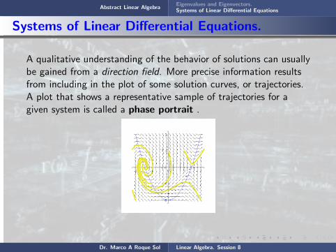

Abstract Linear AlgebraEigenvalues and Eigenvectors.Systems of Linear Differential Equations
Systems of Linear Differential Equations.
Now, for the system
x′ = Ax
we look for solutions of the form
x = veλt
where the exponent λ and the vector v are to be determined.Substituting x in the system gives
λveλt = Aveλt
(A− λI) v = 0
Dr. Marco A Roque Sol Linear Algebra. Session 8

Abstract Linear AlgebraEigenvalues and Eigenvectors.Systems of Linear Differential Equations
Systems of Linear Differential Equations.
Now, for the system
x′ = Ax
we look
for solutions of the form
x = veλt
where the exponent λ and the vector v are to be determined.Substituting x in the system gives
λveλt = Aveλt
(A− λI) v = 0
Dr. Marco A Roque Sol Linear Algebra. Session 8
Abstract Linear AlgebraEigenvalues and Eigenvectors.Systems of Linear Differential Equations
Systems of Linear Differential Equations.
Now, for the system
x′ = Ax
we look for solutions
of the form
x = veλt
where the exponent λ and the vector v are to be determined.Substituting x in the system gives
λveλt = Aveλt
(A− λI) v = 0
Dr. Marco A Roque Sol Linear Algebra. Session 8

Abstract Linear AlgebraEigenvalues and Eigenvectors.Systems of Linear Differential Equations
Systems of Linear Differential Equations.
Now, for the system
x′ = Ax
we look for solutions of the form
x = veλt
where the exponent λ and the vector v are to be determined.Substituting x in the system gives
λveλt = Aveλt
(A− λI) v = 0
Dr. Marco A Roque Sol Linear Algebra. Session 8

Abstract Linear AlgebraEigenvalues and Eigenvectors.Systems of Linear Differential Equations
Systems of Linear Differential Equations.
Now, for the system
x′ = Ax
we look for solutions of the form
x = veλt
where the exponent
λ and the vector v are to be determined.Substituting x in the system gives
λveλt = Aveλt
(A− λI) v = 0
Dr. Marco A Roque Sol Linear Algebra. Session 8

Abstract Linear AlgebraEigenvalues and Eigenvectors.Systems of Linear Differential Equations
Systems of Linear Differential Equations.
Now, for the system
x′ = Ax
we look for solutions of the form
x = veλt
where the exponent λ and
the vector v are to be determined.Substituting x in the system gives
λveλt = Aveλt
(A− λI) v = 0
Dr. Marco A Roque Sol Linear Algebra. Session 8

Abstract Linear AlgebraEigenvalues and Eigenvectors.Systems of Linear Differential Equations
Systems of Linear Differential Equations.
Now, for the system
x′ = Ax
we look for solutions of the form
x = veλt
where the exponent λ and the vector v
are to be determined.Substituting x in the system gives
λveλt = Aveλt
(A− λI) v = 0
Dr. Marco A Roque Sol Linear Algebra. Session 8

Abstract Linear AlgebraEigenvalues and Eigenvectors.Systems of Linear Differential Equations
Systems of Linear Differential Equations.
Now, for the system
x′ = Ax
we look for solutions of the form
x = veλt
where the exponent λ and the vector v are to be
determined.Substituting x in the system gives
λveλt = Aveλt
(A− λI) v = 0
Dr. Marco A Roque Sol Linear Algebra. Session 8
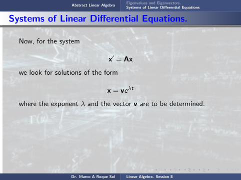
Abstract Linear AlgebraEigenvalues and Eigenvectors.Systems of Linear Differential Equations
Systems of Linear Differential Equations.
Now, for the system
x′ = Ax
we look for solutions of the form
x = veλt
where the exponent λ and the vector v are to be determined.
Substituting x in the system gives
λveλt = Aveλt
(A− λI) v = 0
Dr. Marco A Roque Sol Linear Algebra. Session 8

Abstract Linear AlgebraEigenvalues and Eigenvectors.Systems of Linear Differential Equations
Systems of Linear Differential Equations.
Now, for the system
x′ = Ax
we look for solutions of the form
x = veλt
where the exponent λ and the vector v are to be determined.Substituting x
in the system gives
λveλt = Aveλt
(A− λI) v = 0
Dr. Marco A Roque Sol Linear Algebra. Session 8
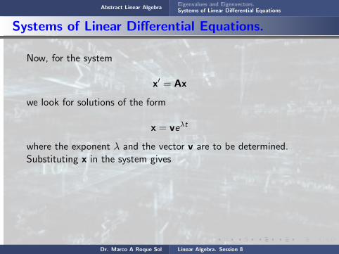
Abstract Linear AlgebraEigenvalues and Eigenvectors.Systems of Linear Differential Equations
Systems of Linear Differential Equations.
Now, for the system
x′ = Ax
we look for solutions of the form
x = veλt
where the exponent λ and the vector v are to be determined.Substituting x in the system gives
λveλt = Aveλt
(A− λI) v = 0
Dr. Marco A Roque Sol Linear Algebra. Session 8
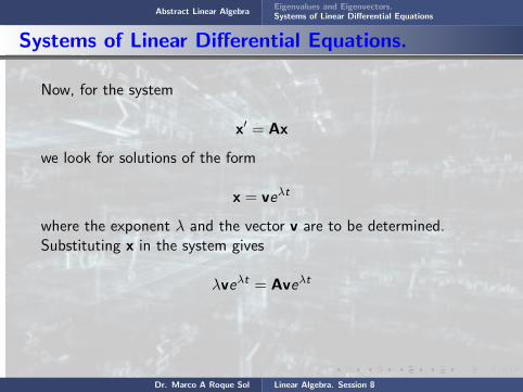
Abstract Linear AlgebraEigenvalues and Eigenvectors.Systems of Linear Differential Equations
Systems of Linear Differential Equations.
Now, for the system
x′ = Ax
we look for solutions of the form
x = veλt
where the exponent λ and the vector v are to be determined.Substituting x in the system gives
λveλt = Aveλt
(A− λI) v = 0
Dr. Marco A Roque Sol Linear Algebra. Session 8
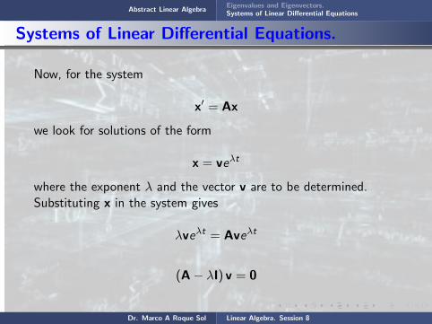
Abstract Linear AlgebraEigenvalues and Eigenvectors.Systems of Linear Differential Equations
Systems of Linear Differential Equations.
Now, for the system
x′ = Ax
we look for solutions of the form
x = veλt
where the exponent λ and the vector v are to be determined.Substituting x in the system gives
λveλt = Aveλt
(A− λI) v = 0
Dr. Marco A Roque Sol Linear Algebra. Session 8

Abstract Linear AlgebraEigenvalues and Eigenvectors.Systems of Linear Differential Equations
Systems of Linear Differential Equations.
Thus, to solve the system of differential equations, we must solvethe above system of algebraic equations. That is, we need to findthe eigenvalues and eigenvectors of the matrix A.
If we assume that A is a real-valued matrix, then we must considerthe following possibilities for the eigenvalues of A:
1. All eigenvalues are real and different from each other.
2. Some eigenvalues occur in complex conjugate pairs.
3. Some eigenvalues, either real or complex, are repeated.
Dr. Marco A Roque Sol Linear Algebra. Session 8

Abstract Linear AlgebraEigenvalues and Eigenvectors.Systems of Linear Differential Equations
Systems of Linear Differential Equations.
Thus,
to solve the system of differential equations, we must solvethe above system of algebraic equations. That is, we need to findthe eigenvalues and eigenvectors of the matrix A.
If we assume that A is a real-valued matrix, then we must considerthe following possibilities for the eigenvalues of A:
1. All eigenvalues are real and different from each other.
2. Some eigenvalues occur in complex conjugate pairs.
3. Some eigenvalues, either real or complex, are repeated.
Dr. Marco A Roque Sol Linear Algebra. Session 8

Abstract Linear AlgebraEigenvalues and Eigenvectors.Systems of Linear Differential Equations
Systems of Linear Differential Equations.
Thus, to solve
the system of differential equations, we must solvethe above system of algebraic equations. That is, we need to findthe eigenvalues and eigenvectors of the matrix A.
If we assume that A is a real-valued matrix, then we must considerthe following possibilities for the eigenvalues of A:
1. All eigenvalues are real and different from each other.
2. Some eigenvalues occur in complex conjugate pairs.
3. Some eigenvalues, either real or complex, are repeated.
Dr. Marco A Roque Sol Linear Algebra. Session 8
Abstract Linear AlgebraEigenvalues and Eigenvectors.Systems of Linear Differential Equations
Systems of Linear Differential Equations.
Thus, to solve the system
of differential equations, we must solvethe above system of algebraic equations. That is, we need to findthe eigenvalues and eigenvectors of the matrix A.
If we assume that A is a real-valued matrix, then we must considerthe following possibilities for the eigenvalues of A:
1. All eigenvalues are real and different from each other.
2. Some eigenvalues occur in complex conjugate pairs.
3. Some eigenvalues, either real or complex, are repeated.
Dr. Marco A Roque Sol Linear Algebra. Session 8
Abstract Linear AlgebraEigenvalues and Eigenvectors.Systems of Linear Differential Equations
Systems of Linear Differential Equations.
Thus, to solve the system of differential equations,
we must solvethe above system of algebraic equations. That is, we need to findthe eigenvalues and eigenvectors of the matrix A.
If we assume that A is a real-valued matrix, then we must considerthe following possibilities for the eigenvalues of A:
1. All eigenvalues are real and different from each other.
2. Some eigenvalues occur in complex conjugate pairs.
3. Some eigenvalues, either real or complex, are repeated.
Dr. Marco A Roque Sol Linear Algebra. Session 8
Abstract Linear AlgebraEigenvalues and Eigenvectors.Systems of Linear Differential Equations
Systems of Linear Differential Equations.
Thus, to solve the system of differential equations, we must solve
the above system of algebraic equations. That is, we need to findthe eigenvalues and eigenvectors of the matrix A.
If we assume that A is a real-valued matrix, then we must considerthe following possibilities for the eigenvalues of A:
1. All eigenvalues are real and different from each other.
2. Some eigenvalues occur in complex conjugate pairs.
3. Some eigenvalues, either real or complex, are repeated.
Dr. Marco A Roque Sol Linear Algebra. Session 8
Abstract Linear AlgebraEigenvalues and Eigenvectors.Systems of Linear Differential Equations
Systems of Linear Differential Equations.
Thus, to solve the system of differential equations, we must solvethe above system
of algebraic equations. That is, we need to findthe eigenvalues and eigenvectors of the matrix A.
If we assume that A is a real-valued matrix, then we must considerthe following possibilities for the eigenvalues of A:
1. All eigenvalues are real and different from each other.
2. Some eigenvalues occur in complex conjugate pairs.
3. Some eigenvalues, either real or complex, are repeated.
Dr. Marco A Roque Sol Linear Algebra. Session 8
Abstract Linear AlgebraEigenvalues and Eigenvectors.Systems of Linear Differential Equations
Systems of Linear Differential Equations.
Thus, to solve the system of differential equations, we must solvethe above system of algebraic equations.
That is, we need to findthe eigenvalues and eigenvectors of the matrix A.
If we assume that A is a real-valued matrix, then we must considerthe following possibilities for the eigenvalues of A:
1. All eigenvalues are real and different from each other.
2. Some eigenvalues occur in complex conjugate pairs.
3. Some eigenvalues, either real or complex, are repeated.
Dr. Marco A Roque Sol Linear Algebra. Session 8
Abstract Linear AlgebraEigenvalues and Eigenvectors.Systems of Linear Differential Equations
Systems of Linear Differential Equations.
Thus, to solve the system of differential equations, we must solvethe above system of algebraic equations. That is,
we need to findthe eigenvalues and eigenvectors of the matrix A.
If we assume that A is a real-valued matrix, then we must considerthe following possibilities for the eigenvalues of A:
1. All eigenvalues are real and different from each other.
2. Some eigenvalues occur in complex conjugate pairs.
3. Some eigenvalues, either real or complex, are repeated.
Dr. Marco A Roque Sol Linear Algebra. Session 8

Abstract Linear AlgebraEigenvalues and Eigenvectors.Systems of Linear Differential Equations
Systems of Linear Differential Equations.
Thus, to solve the system of differential equations, we must solvethe above system of algebraic equations. That is, we need to find
the eigenvalues and eigenvectors of the matrix A.
If we assume that A is a real-valued matrix, then we must considerthe following possibilities for the eigenvalues of A:
1. All eigenvalues are real and different from each other.
2. Some eigenvalues occur in complex conjugate pairs.
3. Some eigenvalues, either real or complex, are repeated.
Dr. Marco A Roque Sol Linear Algebra. Session 8
Abstract Linear AlgebraEigenvalues and Eigenvectors.Systems of Linear Differential Equations
Systems of Linear Differential Equations.
Thus, to solve the system of differential equations, we must solvethe above system of algebraic equations. That is, we need to findthe eigenvalues and
eigenvectors of the matrix A.
If we assume that A is a real-valued matrix, then we must considerthe following possibilities for the eigenvalues of A:
1. All eigenvalues are real and different from each other.
2. Some eigenvalues occur in complex conjugate pairs.
3. Some eigenvalues, either real or complex, are repeated.
Dr. Marco A Roque Sol Linear Algebra. Session 8

Abstract Linear AlgebraEigenvalues and Eigenvectors.Systems of Linear Differential Equations
Systems of Linear Differential Equations.
Thus, to solve the system of differential equations, we must solvethe above system of algebraic equations. That is, we need to findthe eigenvalues and eigenvectors
of the matrix A.
If we assume that A is a real-valued matrix, then we must considerthe following possibilities for the eigenvalues of A:
1. All eigenvalues are real and different from each other.
2. Some eigenvalues occur in complex conjugate pairs.
3. Some eigenvalues, either real or complex, are repeated.
Dr. Marco A Roque Sol Linear Algebra. Session 8

Abstract Linear AlgebraEigenvalues and Eigenvectors.Systems of Linear Differential Equations
Systems of Linear Differential Equations.
Thus, to solve the system of differential equations, we must solvethe above system of algebraic equations. That is, we need to findthe eigenvalues and eigenvectors of the matrix A.
If we assume that A is a real-valued matrix, then we must considerthe following possibilities for the eigenvalues of A:
1. All eigenvalues are real and different from each other.
2. Some eigenvalues occur in complex conjugate pairs.
3. Some eigenvalues, either real or complex, are repeated.
Dr. Marco A Roque Sol Linear Algebra. Session 8

Abstract Linear AlgebraEigenvalues and Eigenvectors.Systems of Linear Differential Equations
Systems of Linear Differential Equations.
Thus, to solve the system of differential equations, we must solvethe above system of algebraic equations. That is, we need to findthe eigenvalues and eigenvectors of the matrix A.
If we assume
that A is a real-valued matrix, then we must considerthe following possibilities for the eigenvalues of A:
1. All eigenvalues are real and different from each other.
2. Some eigenvalues occur in complex conjugate pairs.
3. Some eigenvalues, either real or complex, are repeated.
Dr. Marco A Roque Sol Linear Algebra. Session 8

Abstract Linear AlgebraEigenvalues and Eigenvectors.Systems of Linear Differential Equations
Systems of Linear Differential Equations.
Thus, to solve the system of differential equations, we must solvethe above system of algebraic equations. That is, we need to findthe eigenvalues and eigenvectors of the matrix A.
If we assume that A
is a real-valued matrix, then we must considerthe following possibilities for the eigenvalues of A:
1. All eigenvalues are real and different from each other.
2. Some eigenvalues occur in complex conjugate pairs.
3. Some eigenvalues, either real or complex, are repeated.
Dr. Marco A Roque Sol Linear Algebra. Session 8

Abstract Linear AlgebraEigenvalues and Eigenvectors.Systems of Linear Differential Equations
Systems of Linear Differential Equations.
Thus, to solve the system of differential equations, we must solvethe above system of algebraic equations. That is, we need to findthe eigenvalues and eigenvectors of the matrix A.
If we assume that A is a real-valued matrix,
then we must considerthe following possibilities for the eigenvalues of A:
1. All eigenvalues are real and different from each other.
2. Some eigenvalues occur in complex conjugate pairs.
3. Some eigenvalues, either real or complex, are repeated.
Dr. Marco A Roque Sol Linear Algebra. Session 8

Abstract Linear AlgebraEigenvalues and Eigenvectors.Systems of Linear Differential Equations
Systems of Linear Differential Equations.
Thus, to solve the system of differential equations, we must solvethe above system of algebraic equations. That is, we need to findthe eigenvalues and eigenvectors of the matrix A.
If we assume that A is a real-valued matrix, then we must consider
the following possibilities for the eigenvalues of A:
1. All eigenvalues are real and different from each other.
2. Some eigenvalues occur in complex conjugate pairs.
3. Some eigenvalues, either real or complex, are repeated.
Dr. Marco A Roque Sol Linear Algebra. Session 8
Abstract Linear AlgebraEigenvalues and Eigenvectors.Systems of Linear Differential Equations
Systems of Linear Differential Equations.
Thus, to solve the system of differential equations, we must solvethe above system of algebraic equations. That is, we need to findthe eigenvalues and eigenvectors of the matrix A.
If we assume that A is a real-valued matrix, then we must considerthe following possibilities
for the eigenvalues of A:
1. All eigenvalues are real and different from each other.
2. Some eigenvalues occur in complex conjugate pairs.
3. Some eigenvalues, either real or complex, are repeated.
Dr. Marco A Roque Sol Linear Algebra. Session 8

Abstract Linear AlgebraEigenvalues and Eigenvectors.Systems of Linear Differential Equations
Systems of Linear Differential Equations.
Thus, to solve the system of differential equations, we must solvethe above system of algebraic equations. That is, we need to findthe eigenvalues and eigenvectors of the matrix A.
If we assume that A is a real-valued matrix, then we must considerthe following possibilities for the eigenvalues
of A:
1. All eigenvalues are real and different from each other.
2. Some eigenvalues occur in complex conjugate pairs.
3. Some eigenvalues, either real or complex, are repeated.
Dr. Marco A Roque Sol Linear Algebra. Session 8

Abstract Linear AlgebraEigenvalues and Eigenvectors.Systems of Linear Differential Equations
Systems of Linear Differential Equations.
Thus, to solve the system of differential equations, we must solvethe above system of algebraic equations. That is, we need to findthe eigenvalues and eigenvectors of the matrix A.
If we assume that A is a real-valued matrix, then we must considerthe following possibilities for the eigenvalues of A:
1. All eigenvalues are real and different from each other.
2. Some eigenvalues occur in complex conjugate pairs.
3. Some eigenvalues, either real or complex, are repeated.
Dr. Marco A Roque Sol Linear Algebra. Session 8

Abstract Linear AlgebraEigenvalues and Eigenvectors.Systems of Linear Differential Equations
Systems of Linear Differential Equations.
Thus, to solve the system of differential equations, we must solvethe above system of algebraic equations. That is, we need to findthe eigenvalues and eigenvectors of the matrix A.
If we assume that A is a real-valued matrix, then we must considerthe following possibilities for the eigenvalues of A:
1. All eigenvalues
are real and different from each other.
2. Some eigenvalues occur in complex conjugate pairs.
3. Some eigenvalues, either real or complex, are repeated.
Dr. Marco A Roque Sol Linear Algebra. Session 8

Abstract Linear AlgebraEigenvalues and Eigenvectors.Systems of Linear Differential Equations
Systems of Linear Differential Equations.
Thus, to solve the system of differential equations, we must solvethe above system of algebraic equations. That is, we need to findthe eigenvalues and eigenvectors of the matrix A.
If we assume that A is a real-valued matrix, then we must considerthe following possibilities for the eigenvalues of A:
1. All eigenvalues are real and
different from each other.
2. Some eigenvalues occur in complex conjugate pairs.
3. Some eigenvalues, either real or complex, are repeated.
Dr. Marco A Roque Sol Linear Algebra. Session 8

Abstract Linear AlgebraEigenvalues and Eigenvectors.Systems of Linear Differential Equations
Systems of Linear Differential Equations.
Thus, to solve the system of differential equations, we must solvethe above system of algebraic equations. That is, we need to findthe eigenvalues and eigenvectors of the matrix A.
If we assume that A is a real-valued matrix, then we must considerthe following possibilities for the eigenvalues of A:
1. All eigenvalues are real and different
from each other.
2. Some eigenvalues occur in complex conjugate pairs.
3. Some eigenvalues, either real or complex, are repeated.
Dr. Marco A Roque Sol Linear Algebra. Session 8

Abstract Linear AlgebraEigenvalues and Eigenvectors.Systems of Linear Differential Equations
Systems of Linear Differential Equations.
Thus, to solve the system of differential equations, we must solvethe above system of algebraic equations. That is, we need to findthe eigenvalues and eigenvectors of the matrix A.
If we assume that A is a real-valued matrix, then we must considerthe following possibilities for the eigenvalues of A:
1. All eigenvalues are real and different from each other.
2. Some eigenvalues occur in complex conjugate pairs.
3. Some eigenvalues, either real or complex, are repeated.
Dr. Marco A Roque Sol Linear Algebra. Session 8

Abstract Linear AlgebraEigenvalues and Eigenvectors.Systems of Linear Differential Equations
Systems of Linear Differential Equations.
Thus, to solve the system of differential equations, we must solvethe above system of algebraic equations. That is, we need to findthe eigenvalues and eigenvectors of the matrix A.
If we assume that A is a real-valued matrix, then we must considerthe following possibilities for the eigenvalues of A:
1. All eigenvalues are real and different from each other.
2. Some eigenvalues
occur in complex conjugate pairs.
3. Some eigenvalues, either real or complex, are repeated.
Dr. Marco A Roque Sol Linear Algebra. Session 8

Abstract Linear AlgebraEigenvalues and Eigenvectors.Systems of Linear Differential Equations
Systems of Linear Differential Equations.
Thus, to solve the system of differential equations, we must solvethe above system of algebraic equations. That is, we need to findthe eigenvalues and eigenvectors of the matrix A.
If we assume that A is a real-valued matrix, then we must considerthe following possibilities for the eigenvalues of A:
1. All eigenvalues are real and different from each other.
2. Some eigenvalues occur in
complex conjugate pairs.
3. Some eigenvalues, either real or complex, are repeated.
Dr. Marco A Roque Sol Linear Algebra. Session 8

Abstract Linear AlgebraEigenvalues and Eigenvectors.Systems of Linear Differential Equations
Systems of Linear Differential Equations.
Thus, to solve the system of differential equations, we must solvethe above system of algebraic equations. That is, we need to findthe eigenvalues and eigenvectors of the matrix A.
If we assume that A is a real-valued matrix, then we must considerthe following possibilities for the eigenvalues of A:
1. All eigenvalues are real and different from each other.
2. Some eigenvalues occur in complex conjugate pairs.
3. Some eigenvalues, either real or complex, are repeated.
Dr. Marco A Roque Sol Linear Algebra. Session 8
Abstract Linear AlgebraEigenvalues and Eigenvectors.Systems of Linear Differential Equations
Systems of Linear Differential Equations.
Thus, to solve the system of differential equations, we must solvethe above system of algebraic equations. That is, we need to findthe eigenvalues and eigenvectors of the matrix A.
If we assume that A is a real-valued matrix, then we must considerthe following possibilities for the eigenvalues of A:
1. All eigenvalues are real and different from each other.
2. Some eigenvalues occur in complex conjugate pairs.
3. Some eigenvalues,
either real or complex, are repeated.
Dr. Marco A Roque Sol Linear Algebra. Session 8

Abstract Linear AlgebraEigenvalues and Eigenvectors.Systems of Linear Differential Equations
Systems of Linear Differential Equations.
Thus, to solve the system of differential equations, we must solvethe above system of algebraic equations. That is, we need to findthe eigenvalues and eigenvectors of the matrix A.
If we assume that A is a real-valued matrix, then we must considerthe following possibilities for the eigenvalues of A:
1. All eigenvalues are real and different from each other.
2. Some eigenvalues occur in complex conjugate pairs.
3. Some eigenvalues, either real or
complex, are repeated.
Dr. Marco A Roque Sol Linear Algebra. Session 8

Abstract Linear AlgebraEigenvalues and Eigenvectors.Systems of Linear Differential Equations
Systems of Linear Differential Equations.
Thus, to solve the system of differential equations, we must solvethe above system of algebraic equations. That is, we need to findthe eigenvalues and eigenvectors of the matrix A.
If we assume that A is a real-valued matrix, then we must considerthe following possibilities for the eigenvalues of A:
1. All eigenvalues are real and different from each other.
2. Some eigenvalues occur in complex conjugate pairs.
3. Some eigenvalues, either real or complex,
are repeated.
Dr. Marco A Roque Sol Linear Algebra. Session 8

Abstract Linear AlgebraEigenvalues and Eigenvectors.Systems of Linear Differential Equations
Systems of Linear Differential Equations.
Thus, to solve the system of differential equations, we must solvethe above system of algebraic equations. That is, we need to findthe eigenvalues and eigenvectors of the matrix A.
If we assume that A is a real-valued matrix, then we must considerthe following possibilities for the eigenvalues of A:
1. All eigenvalues are real and different from each other.
2. Some eigenvalues occur in complex conjugate pairs.
3. Some eigenvalues, either real or complex, are repeated.
Dr. Marco A Roque Sol Linear Algebra. Session 8

Abstract Linear AlgebraEigenvalues and Eigenvectors.Systems of Linear Differential Equations
Systems of Linear Differential Equations.
Example 9.5
Consider the system
x′ = Ax =
(1 14 1
)x
Solution
Let’s find the eigenvalues of the matrix A
Dr. Marco A Roque Sol Linear Algebra. Session 8

Abstract Linear AlgebraEigenvalues and Eigenvectors.Systems of Linear Differential Equations
Systems of Linear Differential Equations.
Example 9.5
Consider the system
x′ = Ax =
(1 14 1
)x
Solution
Let’s find the eigenvalues of the matrix A
Dr. Marco A Roque Sol Linear Algebra. Session 8

Abstract Linear AlgebraEigenvalues and Eigenvectors.Systems of Linear Differential Equations
Systems of Linear Differential Equations.
Example 9.5
Consider
the system
x′ = Ax =
(1 14 1
)x
Solution
Let’s find the eigenvalues of the matrix A
Dr. Marco A Roque Sol Linear Algebra. Session 8

Abstract Linear AlgebraEigenvalues and Eigenvectors.Systems of Linear Differential Equations
Systems of Linear Differential Equations.
Example 9.5
Consider the system
x′ = Ax =
(1 14 1
)x
Solution
Let’s find the eigenvalues of the matrix A
Dr. Marco A Roque Sol Linear Algebra. Session 8
Abstract Linear AlgebraEigenvalues and Eigenvectors.Systems of Linear Differential Equations
Systems of Linear Differential Equations.
Example 9.5
Consider the system
x′ = Ax =
(1 14 1
)x
Solution
Let’s find the eigenvalues of the matrix A
Dr. Marco A Roque Sol Linear Algebra. Session 8
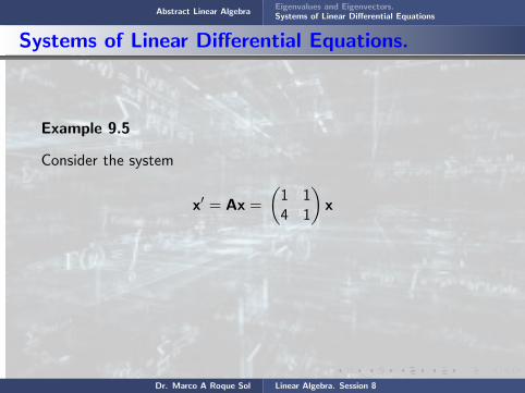
Abstract Linear AlgebraEigenvalues and Eigenvectors.Systems of Linear Differential Equations
Systems of Linear Differential Equations.
Example 9.5
Consider the system
x′ = Ax =
(1 14 1
)x
Solution
Let’s find the eigenvalues of the matrix A
Dr. Marco A Roque Sol Linear Algebra. Session 8

Abstract Linear AlgebraEigenvalues and Eigenvectors.Systems of Linear Differential Equations
Systems of Linear Differential Equations.
Example 9.5
Consider the system
x′ = Ax =
(1 14 1
)x
Solution
Let’s find the eigenvalues of the matrix A
Dr. Marco A Roque Sol Linear Algebra. Session 8

Abstract Linear AlgebraEigenvalues and Eigenvectors.Systems of Linear Differential Equations
Systems of Linear Differential Equations.
Example 9.5
Consider the system
x′ = Ax =
(1 14 1
)x
Solution
Let’s find
the eigenvalues of the matrix A
Dr. Marco A Roque Sol Linear Algebra. Session 8

Abstract Linear AlgebraEigenvalues and Eigenvectors.Systems of Linear Differential Equations
Systems of Linear Differential Equations.
Example 9.5
Consider the system
x′ = Ax =
(1 14 1
)x
Solution
Let’s find the eigenvalues
of the matrix A
Dr. Marco A Roque Sol Linear Algebra. Session 8

Abstract Linear AlgebraEigenvalues and Eigenvectors.Systems of Linear Differential Equations
Systems of Linear Differential Equations.
Example 9.5
Consider the system
x′ = Ax =
(1 14 1
)x
Solution
Let’s find the eigenvalues of the matrix
A
Dr. Marco A Roque Sol Linear Algebra. Session 8

Abstract Linear AlgebraEigenvalues and Eigenvectors.Systems of Linear Differential Equations
Systems of Linear Differential Equations.
Example 9.5
Consider the system
x′ = Ax =
(1 14 1
)x
Solution
Let’s find the eigenvalues of the matrix A
Dr. Marco A Roque Sol Linear Algebra. Session 8

Abstract Linear AlgebraEigenvalues and Eigenvectors.Systems of Linear Differential Equations
Systems of Linear Differential Equations.
|A− λI| =
∣∣∣∣1− λ 14 1− λ
∣∣∣∣ = 0
(1− λ)2 − 4 = 0 =⇒
(λ2 − 2λ− 3 = (λ− 3)(λ+ 1) = 0 =⇒
Dr. Marco A Roque Sol Linear Algebra. Session 8

Abstract Linear AlgebraEigenvalues and Eigenvectors.Systems of Linear Differential Equations
Systems of Linear Differential Equations.
|A− λI| =
∣∣∣∣1− λ 14 1− λ
∣∣∣∣ = 0
(1− λ)2 − 4 = 0 =⇒
(λ2 − 2λ− 3 = (λ− 3)(λ+ 1) = 0 =⇒
Dr. Marco A Roque Sol Linear Algebra. Session 8
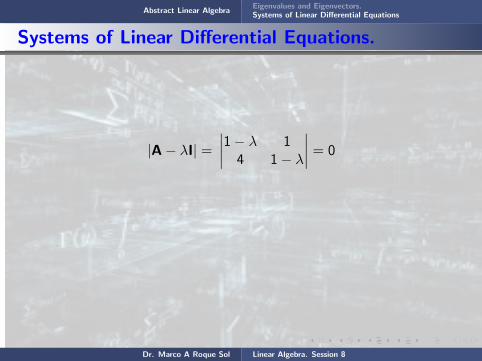
Abstract Linear AlgebraEigenvalues and Eigenvectors.Systems of Linear Differential Equations
Systems of Linear Differential Equations.
|A− λI| =
∣∣∣∣1− λ 14 1− λ
∣∣∣∣ = 0
(1− λ)2 − 4 = 0 =⇒
(λ2 − 2λ− 3 = (λ− 3)(λ+ 1) = 0 =⇒
Dr. Marco A Roque Sol Linear Algebra. Session 8

Abstract Linear AlgebraEigenvalues and Eigenvectors.Systems of Linear Differential Equations
Systems of Linear Differential Equations.
|A− λI| =
∣∣∣∣1− λ 14 1− λ
∣∣∣∣ = 0
(1− λ)2 − 4 = 0 =⇒
(λ2 − 2λ− 3 = (λ− 3)(λ+ 1) = 0 =⇒
Dr. Marco A Roque Sol Linear Algebra. Session 8

Abstract Linear AlgebraEigenvalues and Eigenvectors.Systems of Linear Differential Equations
Systems of Linear Differential Equations.
|A− λI| =
∣∣∣∣1− λ 14 1− λ
∣∣∣∣ = 0
(1− λ)2 − 4 = 0 =⇒
(λ2 − 2λ− 3 = (λ− 3)(λ+ 1) = 0 =⇒
Dr. Marco A Roque Sol Linear Algebra. Session 8

Abstract Linear AlgebraEigenvalues and Eigenvectors.Systems of Linear Differential Equations
Systems of Linear Differential Equations.
λ1 = 3, λ2 = −1
If λ1 = 3, then the system reduces to the single equation
−2v1 + v2 = 0, =⇒ v2 = 2v1
and a corresponding eigenvector is
v(1) =
(12
)
Dr. Marco A Roque Sol Linear Algebra. Session 8

Abstract Linear AlgebraEigenvalues and Eigenvectors.Systems of Linear Differential Equations
Systems of Linear Differential Equations.
λ1 = 3, λ2 = −1
If λ1 = 3,
then the system reduces to the single equation
−2v1 + v2 = 0, =⇒ v2 = 2v1
and a corresponding eigenvector is
v(1) =
(12
)
Dr. Marco A Roque Sol Linear Algebra. Session 8
Abstract Linear AlgebraEigenvalues and Eigenvectors.Systems of Linear Differential Equations
Systems of Linear Differential Equations.
λ1 = 3, λ2 = −1
If λ1 = 3, then the system
reduces to the single equation
−2v1 + v2 = 0, =⇒ v2 = 2v1
and a corresponding eigenvector is
v(1) =
(12
)
Dr. Marco A Roque Sol Linear Algebra. Session 8
Abstract Linear AlgebraEigenvalues and Eigenvectors.Systems of Linear Differential Equations
Systems of Linear Differential Equations.
λ1 = 3, λ2 = −1
If λ1 = 3, then the system reduces to
the single equation
−2v1 + v2 = 0, =⇒ v2 = 2v1
and a corresponding eigenvector is
v(1) =
(12
)
Dr. Marco A Roque Sol Linear Algebra. Session 8

Abstract Linear AlgebraEigenvalues and Eigenvectors.Systems of Linear Differential Equations
Systems of Linear Differential Equations.
λ1 = 3, λ2 = −1
If λ1 = 3, then the system reduces to the single equation
−2v1 + v2 = 0, =⇒ v2 = 2v1
and a corresponding eigenvector is
v(1) =
(12
)
Dr. Marco A Roque Sol Linear Algebra. Session 8

Abstract Linear AlgebraEigenvalues and Eigenvectors.Systems of Linear Differential Equations
Systems of Linear Differential Equations.
λ1 = 3, λ2 = −1
If λ1 = 3, then the system reduces to the single equation
−2v1 + v2 = 0, =⇒ v2 = 2v1
and a corresponding eigenvector is
v(1) =
(12
)
Dr. Marco A Roque Sol Linear Algebra. Session 8
Abstract Linear AlgebraEigenvalues and Eigenvectors.Systems of Linear Differential Equations
Systems of Linear Differential Equations.
λ1 = 3, λ2 = −1
If λ1 = 3, then the system reduces to the single equation
−2v1 + v2 = 0, =⇒ v2 = 2v1
and
a corresponding eigenvector is
v(1) =
(12
)
Dr. Marco A Roque Sol Linear Algebra. Session 8
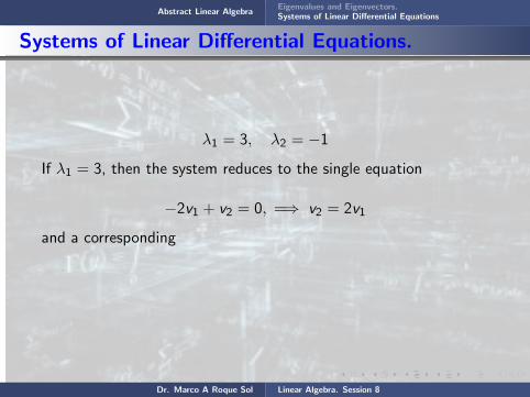
Abstract Linear AlgebraEigenvalues and Eigenvectors.Systems of Linear Differential Equations
Systems of Linear Differential Equations.
λ1 = 3, λ2 = −1
If λ1 = 3, then the system reduces to the single equation
−2v1 + v2 = 0, =⇒ v2 = 2v1
and a corresponding
eigenvector is
v(1) =
(12
)
Dr. Marco A Roque Sol Linear Algebra. Session 8

Abstract Linear AlgebraEigenvalues and Eigenvectors.Systems of Linear Differential Equations
Systems of Linear Differential Equations.
λ1 = 3, λ2 = −1
If λ1 = 3, then the system reduces to the single equation
−2v1 + v2 = 0, =⇒ v2 = 2v1
and a corresponding eigenvector is
v(1) =
(12
)
Dr. Marco A Roque Sol Linear Algebra. Session 8
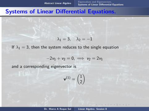

Abstract Linear AlgebraEigenvalues and Eigenvectors.Systems of Linear Differential Equations
Systems of Linear Differential Equations.
Similarly, corresponding to λ2 = −1, we find that a correspondingeigenvector is
v(2) =
(1
− 2
)The corresponding solutions of the differential equation are
x(1) =
(12
)e3t ; x(2) =
(1
− 2
)e−t
Dr. Marco A Roque Sol Linear Algebra. Session 8

Abstract Linear AlgebraEigenvalues and Eigenvectors.Systems of Linear Differential Equations
Systems of Linear Differential Equations.
Similarly,
corresponding to λ2 = −1, we find that a correspondingeigenvector is
v(2) =
(1
− 2
)The corresponding solutions of the differential equation are
x(1) =
(12
)e3t ; x(2) =
(1
− 2
)e−t
Dr. Marco A Roque Sol Linear Algebra. Session 8
Abstract Linear AlgebraEigenvalues and Eigenvectors.Systems of Linear Differential Equations
Systems of Linear Differential Equations.
Similarly, corresponding to λ2 = −1,
we find that a correspondingeigenvector is
v(2) =
(1
− 2
)The corresponding solutions of the differential equation are
x(1) =
(12
)e3t ; x(2) =
(1
− 2
)e−t
Dr. Marco A Roque Sol Linear Algebra. Session 8
Abstract Linear AlgebraEigenvalues and Eigenvectors.Systems of Linear Differential Equations
Systems of Linear Differential Equations.
Similarly, corresponding to λ2 = −1, we find
that a correspondingeigenvector is
v(2) =
(1
− 2
)The corresponding solutions of the differential equation are
x(1) =
(12
)e3t ; x(2) =
(1
− 2
)e−t
Dr. Marco A Roque Sol Linear Algebra. Session 8
Abstract Linear AlgebraEigenvalues and Eigenvectors.Systems of Linear Differential Equations
Systems of Linear Differential Equations.
Similarly, corresponding to λ2 = −1, we find that a correspondingeigenvector
is
v(2) =
(1
− 2
)The corresponding solutions of the differential equation are
x(1) =
(12
)e3t ; x(2) =
(1
− 2
)e−t
Dr. Marco A Roque Sol Linear Algebra. Session 8

Abstract Linear AlgebraEigenvalues and Eigenvectors.Systems of Linear Differential Equations
Systems of Linear Differential Equations.
Similarly, corresponding to λ2 = −1, we find that a correspondingeigenvector is
v(2) =
(1
− 2
)The corresponding solutions of the differential equation are
x(1) =
(12
)e3t ; x(2) =
(1
− 2
)e−t
Dr. Marco A Roque Sol Linear Algebra. Session 8

Abstract Linear AlgebraEigenvalues and Eigenvectors.Systems of Linear Differential Equations
Systems of Linear Differential Equations.
Similarly, corresponding to λ2 = −1, we find that a correspondingeigenvector is
v(2) =
(1
− 2
)
The corresponding solutions of the differential equation are
x(1) =
(12
)e3t ; x(2) =
(1
− 2
)e−t
Dr. Marco A Roque Sol Linear Algebra. Session 8

Abstract Linear AlgebraEigenvalues and Eigenvectors.Systems of Linear Differential Equations
Systems of Linear Differential Equations.
Similarly, corresponding to λ2 = −1, we find that a correspondingeigenvector is
v(2) =
(1
− 2
)The corresponding solutions
of the differential equation are
x(1) =
(12
)e3t ; x(2) =
(1
− 2
)e−t
Dr. Marco A Roque Sol Linear Algebra. Session 8
Abstract Linear AlgebraEigenvalues and Eigenvectors.Systems of Linear Differential Equations
Systems of Linear Differential Equations.
Similarly, corresponding to λ2 = −1, we find that a correspondingeigenvector is
v(2) =
(1
− 2
)The corresponding solutions of the differential equation
are
x(1) =
(12
)e3t ; x(2) =
(1
− 2
)e−t
Dr. Marco A Roque Sol Linear Algebra. Session 8

Abstract Linear AlgebraEigenvalues and Eigenvectors.Systems of Linear Differential Equations
Systems of Linear Differential Equations.
Similarly, corresponding to λ2 = −1, we find that a correspondingeigenvector is
v(2) =
(1
− 2
)The corresponding solutions of the differential equation are
x(1) =
(12
)e3t ; x(2) =
(1
− 2
)e−t
Dr. Marco A Roque Sol Linear Algebra. Session 8
Abstract Linear AlgebraEigenvalues and Eigenvectors.Systems of Linear Differential Equations
Systems of Linear Differential Equations.
Similarly, corresponding to λ2 = −1, we find that a correspondingeigenvector is
v(2) =
(1
− 2
)The corresponding solutions of the differential equation are
x(1) =
(12
)e3t ;
x(2) =
(1
− 2
)e−t
Dr. Marco A Roque Sol Linear Algebra. Session 8

Abstract Linear AlgebraEigenvalues and Eigenvectors.Systems of Linear Differential Equations
Systems of Linear Differential Equations.
Similarly, corresponding to λ2 = −1, we find that a correspondingeigenvector is
v(2) =
(1
− 2
)The corresponding solutions of the differential equation are
x(1) =
(12
)e3t ; x(2) =
(1
− 2
)e−t
Dr. Marco A Roque Sol Linear Algebra. Session 8
Abstract Linear AlgebraEigenvalues and Eigenvectors.Systems of Linear Differential Equations
Systems of Linear Differential Equations.
The Wronskian of these solutions is
W [x(1), x(2)](t) =
∣∣∣∣ e3t e−t
2e3t −2e−t
∣∣∣∣ = − 4e2t 6= 0
Hence, the solutions x(1) and x(2) form a fundamental set, and thegeneral solution of the system is
x = c1x(1) + c2x(2) = c1
(12
)e3t + c2
(1
− 2
)e−t
Dr. Marco A Roque Sol Linear Algebra. Session 8
Abstract Linear AlgebraEigenvalues and Eigenvectors.Systems of Linear Differential Equations
Systems of Linear Differential Equations.
The Wronskian
of these solutions is
W [x(1), x(2)](t) =
∣∣∣∣ e3t e−t
2e3t −2e−t
∣∣∣∣ = − 4e2t 6= 0
Hence, the solutions x(1) and x(2) form a fundamental set, and thegeneral solution of the system is
x = c1x(1) + c2x(2) = c1
(12
)e3t + c2
(1
− 2
)e−t
Dr. Marco A Roque Sol Linear Algebra. Session 8

Abstract Linear AlgebraEigenvalues and Eigenvectors.Systems of Linear Differential Equations
Systems of Linear Differential Equations.
The Wronskian of these solutions
is
W [x(1), x(2)](t) =
∣∣∣∣ e3t e−t
2e3t −2e−t
∣∣∣∣ = − 4e2t 6= 0
Hence, the solutions x(1) and x(2) form a fundamental set, and thegeneral solution of the system is
x = c1x(1) + c2x(2) = c1
(12
)e3t + c2
(1
− 2
)e−t
Dr. Marco A Roque Sol Linear Algebra. Session 8

Abstract Linear AlgebraEigenvalues and Eigenvectors.Systems of Linear Differential Equations
Systems of Linear Differential Equations.
The Wronskian of these solutions is
W [x(1), x(2)](t) =
∣∣∣∣ e3t e−t
2e3t −2e−t
∣∣∣∣ = − 4e2t 6= 0
Hence, the solutions x(1) and x(2) form a fundamental set, and thegeneral solution of the system is
x = c1x(1) + c2x(2) = c1
(12
)e3t + c2
(1
− 2
)e−t
Dr. Marco A Roque Sol Linear Algebra. Session 8

Abstract Linear AlgebraEigenvalues and Eigenvectors.Systems of Linear Differential Equations
Systems of Linear Differential Equations.
The Wronskian of these solutions is
W [x(1), x(2)](t) =
∣∣∣∣ e3t e−t
2e3t −2e−t
∣∣∣∣ =
− 4e2t 6= 0
Hence, the solutions x(1) and x(2) form a fundamental set, and thegeneral solution of the system is
x = c1x(1) + c2x(2) = c1
(12
)e3t + c2
(1
− 2
)e−t
Dr. Marco A Roque Sol Linear Algebra. Session 8
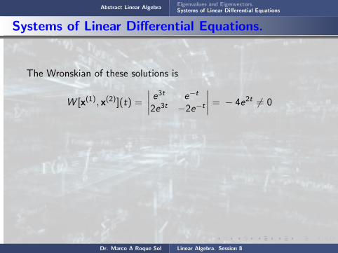
Abstract Linear AlgebraEigenvalues and Eigenvectors.Systems of Linear Differential Equations
Systems of Linear Differential Equations.
The Wronskian of these solutions is
W [x(1), x(2)](t) =
∣∣∣∣ e3t e−t
2e3t −2e−t
∣∣∣∣ = − 4e2t 6= 0
Hence, the solutions x(1) and x(2) form a fundamental set, and thegeneral solution of the system is
x = c1x(1) + c2x(2) = c1
(12
)e3t + c2
(1
− 2
)e−t
Dr. Marco A Roque Sol Linear Algebra. Session 8
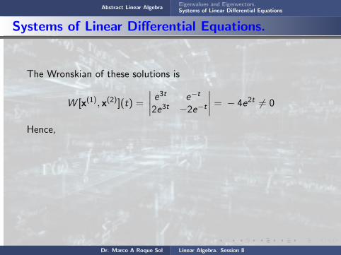
Abstract Linear AlgebraEigenvalues and Eigenvectors.Systems of Linear Differential Equations
Systems of Linear Differential Equations.
The Wronskian of these solutions is
W [x(1), x(2)](t) =
∣∣∣∣ e3t e−t
2e3t −2e−t
∣∣∣∣ = − 4e2t 6= 0
Hence,
the solutions x(1) and x(2) form a fundamental set, and thegeneral solution of the system is
x = c1x(1) + c2x(2) = c1
(12
)e3t + c2
(1
− 2
)e−t
Dr. Marco A Roque Sol Linear Algebra. Session 8

Abstract Linear AlgebraEigenvalues and Eigenvectors.Systems of Linear Differential Equations
Systems of Linear Differential Equations.
The Wronskian of these solutions is
W [x(1), x(2)](t) =
∣∣∣∣ e3t e−t
2e3t −2e−t
∣∣∣∣ = − 4e2t 6= 0
Hence, the solutions
x(1) and x(2) form a fundamental set, and thegeneral solution of the system is
x = c1x(1) + c2x(2) = c1
(12
)e3t + c2
(1
− 2
)e−t
Dr. Marco A Roque Sol Linear Algebra. Session 8

Abstract Linear AlgebraEigenvalues and Eigenvectors.Systems of Linear Differential Equations
Systems of Linear Differential Equations.
The Wronskian of these solutions is
W [x(1), x(2)](t) =
∣∣∣∣ e3t e−t
2e3t −2e−t
∣∣∣∣ = − 4e2t 6= 0
Hence, the solutions x(1) and
x(2) form a fundamental set, and thegeneral solution of the system is
x = c1x(1) + c2x(2) = c1
(12
)e3t + c2
(1
− 2
)e−t
Dr. Marco A Roque Sol Linear Algebra. Session 8

Abstract Linear AlgebraEigenvalues and Eigenvectors.Systems of Linear Differential Equations
Systems of Linear Differential Equations.
The Wronskian of these solutions is
W [x(1), x(2)](t) =
∣∣∣∣ e3t e−t
2e3t −2e−t
∣∣∣∣ = − 4e2t 6= 0
Hence, the solutions x(1) and x(2)
form a fundamental set, and thegeneral solution of the system is
x = c1x(1) + c2x(2) = c1
(12
)e3t + c2
(1
− 2
)e−t
Dr. Marco A Roque Sol Linear Algebra. Session 8
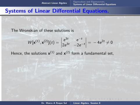
Abstract Linear AlgebraEigenvalues and Eigenvectors.Systems of Linear Differential Equations
Systems of Linear Differential Equations.
The Wronskian of these solutions is
W [x(1), x(2)](t) =
∣∣∣∣ e3t e−t
2e3t −2e−t
∣∣∣∣ = − 4e2t 6= 0
Hence, the solutions x(1) and x(2) form a fundamental set,
and thegeneral solution of the system is
x = c1x(1) + c2x(2) = c1
(12
)e3t + c2
(1
− 2
)e−t
Dr. Marco A Roque Sol Linear Algebra. Session 8
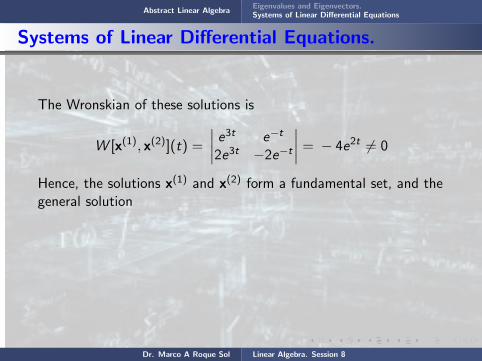
Abstract Linear AlgebraEigenvalues and Eigenvectors.Systems of Linear Differential Equations
Systems of Linear Differential Equations.
The Wronskian of these solutions is
W [x(1), x(2)](t) =
∣∣∣∣ e3t e−t
2e3t −2e−t
∣∣∣∣ = − 4e2t 6= 0
Hence, the solutions x(1) and x(2) form a fundamental set, and thegeneral solution
of the system is
x = c1x(1) + c2x(2) = c1
(12
)e3t + c2
(1
− 2
)e−t
Dr. Marco A Roque Sol Linear Algebra. Session 8

Abstract Linear AlgebraEigenvalues and Eigenvectors.Systems of Linear Differential Equations
Systems of Linear Differential Equations.
The Wronskian of these solutions is
W [x(1), x(2)](t) =
∣∣∣∣ e3t e−t
2e3t −2e−t
∣∣∣∣ = − 4e2t 6= 0
Hence, the solutions x(1) and x(2) form a fundamental set, and thegeneral solution of the system is
x = c1x(1) + c2x(2) = c1
(12
)e3t + c2
(1
− 2
)e−t
Dr. Marco A Roque Sol Linear Algebra. Session 8

Abstract Linear AlgebraEigenvalues and Eigenvectors.Systems of Linear Differential Equations
Systems of Linear Differential Equations.
The Wronskian of these solutions is
W [x(1), x(2)](t) =
∣∣∣∣ e3t e−t
2e3t −2e−t
∣∣∣∣ = − 4e2t 6= 0
Hence, the solutions x(1) and x(2) form a fundamental set, and thegeneral solution of the system is
x =
c1x(1) + c2x(2) = c1
(12
)e3t + c2
(1
− 2
)e−t
Dr. Marco A Roque Sol Linear Algebra. Session 8

Abstract Linear AlgebraEigenvalues and Eigenvectors.Systems of Linear Differential Equations
Systems of Linear Differential Equations.
The Wronskian of these solutions is
W [x(1), x(2)](t) =
∣∣∣∣ e3t e−t
2e3t −2e−t
∣∣∣∣ = − 4e2t 6= 0
Hence, the solutions x(1) and x(2) form a fundamental set, and thegeneral solution of the system is
x = c1x(1) + c2x(2) =
c1
(12
)e3t + c2
(1
− 2
)e−t
Dr. Marco A Roque Sol Linear Algebra. Session 8

Abstract Linear AlgebraEigenvalues and Eigenvectors.Systems of Linear Differential Equations
Systems of Linear Differential Equations.
The Wronskian of these solutions is
W [x(1), x(2)](t) =
∣∣∣∣ e3t e−t
2e3t −2e−t
∣∣∣∣ = − 4e2t 6= 0
Hence, the solutions x(1) and x(2) form a fundamental set, and thegeneral solution of the system is
x = c1x(1) + c2x(2) = c1
(12
)e3t +
c2
(1
− 2
)e−t
Dr. Marco A Roque Sol Linear Algebra. Session 8

Abstract Linear AlgebraEigenvalues and Eigenvectors.Systems of Linear Differential Equations
Systems of Linear Differential Equations.
The Wronskian of these solutions is
W [x(1), x(2)](t) =
∣∣∣∣ e3t e−t
2e3t −2e−t
∣∣∣∣ = − 4e2t 6= 0
Hence, the solutions x(1) and x(2) form a fundamental set, and thegeneral solution of the system is
x = c1x(1) + c2x(2) = c1
(12
)e3t + c2
(1
− 2
)e−t
Dr. Marco A Roque Sol Linear Algebra. Session 8