Embed Size (px)
Citation preview
Linear Algebra for Theoretical Neuroscience (Part 1)Ken Miller
c©2001, 2008 by Kenneth Miller. This work is licensed under the Creative Commons Attribution-Noncommercial-Share Alike 3.0 United States License. To view a copy of this license, visithttp://creativecommons.org/licenses/by-nc-sa/3.0/us/ or send a letter to Creative Commons, 171Second Street, Suite 300, San Francisco, California, 94105, USA.
Current versions of all parts of this work can be found athttp://www.neurotheory.columbia.edu/∼ken/math-notes. Please feel free to link to this site.
I would appreciate any and all feedback that would help improve these notes as a teachingtool – what was particularly helpful, where you got stuck and what might have helped get youunstuck. I already know that more figures, problems, and neurobiological examples are needed ina future incarnation – for the most part I didn’t have time to make figures – but that shouldn’tdiscourage contributions of or suggestions as to useful figures, problems, examples. There are alsomany missing mathematical pieces I would like to fill in, as described on the home page for thesenotes. If anyone wants to turn this into a collaboration and help, I’d be open to discussing thattoo. Feedback can be sent to me by email, [email protected]
Reading These Notes (Instructions as written for classes I’ve taught that usedthese notes)
I have tried to begin at the beginning and make things clear enough that everyone can followassuming basic college math as background. Some of it will be trivial for you; I hope none of itwill be over your head, but some might. My suggested rules for reading this are:
• Read and work through everything. Read with pen and paper beside you. Never let yourselfread through anything you don’t completely understand; work through it until it is crystalclear to you. Go at your own pace; breeze through whatever is trivial for you.
• Do all of the “problems”. Talk among yourselves as much as desired in coming to an un-derstanding of them, but then actually write up the answers by yourself. Most or all of theproblems are very simple; many only require one line as an answer.
If you find a problem to be so obvious for you that it is a waste of your time or annoying towrite it down, go ahead and skip it. But do be conservative in your judgements – it can besurprising how much you can learn by working out in detail what you think you understandin a general way.
You can’t understand the material without doing. In most cases, I have led you step by stepthrough what is required. The purpose of the problems is not to test your math ability, butsimply to make sure you “do” enough to achieve understanding.
• The “exercises” do not require a written answer. But — except where one is prefaced bysomething like “for those interested” — you should read them, make sure you understandthem, and if possible solve them in your head or on paper.
• As you read these notes, mark them with feedback: things you don’t understand, things youget confused by, things that seem trivial or unnecessary, suggestions, whatever. Then turn into me a copy of your annotated notes.
1

References
If you want to consult other references on this material: an excellent text, although fairly math-ematical, is Differential equations, dynamical systems and linear algebra, by Morris W.Hirsch and Steven Smale (Academic Press, NY, 1974). Gilbert Strang has written several very nicetexts that are strong on intuition, including a couple of different linear algebra texts – I’m not sureof their relative strengths and weaknesses – and an Introduction to Applied Mathematics.A good practical reference — sort of a cheat sheet of basic results, plus computer algorithms andpractical advice on doing computations — is Numerical Recipes in C, 2nd Edition, by W.H.Press, S.A. Teukolsky, W.T. Vetterling, and B.P. Flannery (Cambridge University Press, 1992).Part 3 of these notes, which deals with non-normal matrices – matrices that do not have a com-plete orthonormal basis of eigenvectors – needs to be completely rewritten: since it was written,I’ve learned that non-normal matrices have many features not predicted by the eigenvalues thatare of great relevance in neurobiology and in biology more generally, and the notes don’t deal withthis. In the meantime, for mathematical aspects of non-normal matrix behavior, see the book byL.N. Trefethen and M. Embree, Spectra and Pseudospectra: The Behavior of Nonnormal Matricesand Operators. Princeton University Press, 2005.
2
1 Introduction to Vectors and Matrices
We will start out by reviewing basic notation describing, and basic operations of, vectors andmatrices. Why do we care about such things? In neurobiological modeling we are often dealingwith arrays of variables: the activities of all of the neurons in a network at a given time; the firingrate of a neuron in each of many small epochs of time; the weights of all of the synapses impingingon a postsynaptic cell. The natural language for thinking about and analyzing the behavior of sucharrays of variables is the language of vectors and matrices.
1.1 Notation
A scalar is simply a number – we use the term scalar to distinguish numbers from vectors, whichare arrays of numbers. Scalars will be written without boldface: x, y, etc.
We will write a vector as a bold-faced small letter, e.g. v; this denotes a column vector. Itselements vi are written without bold-face:
v =
v0v1. . .vN−1
(1)
Here N , the number of elements, is the dimension of v. The transpose of v, vT, is a row vector:
vT = (v0, v1, . . . , vN−1). (2)
The transpose of a row vector, in turn, is a column vector; in particular, (vT)T = v. Thus, to keepthings easier to write, we can also write v as v = (v0, v1, . . . , vN−1)
T.1
We will write a matrix as a bold-faced capital letter, e.g. M; its elements Mij , where i indicatesthe row and j indicates the column, are written without boldface:
M =
M00 M01 . . . M0(N−1)M10 M11 . . . M1(N−1). . . . . . . . . . . .
M(N−1)0 M(N−1)1 . . . M(N−1)(N−1)
(3)
This is a square, N × N matrix. A matrix can also be rectangular, e.g. a P × N matrix wouldhave P rows and N columns. In particular, an N-dimensional vector can be regarded as an N × 1matrix, while its transpose can be regarded as a 1×N matrix. For the most part, we will only beconcerned with square matrices and with vectors, although we will eventually return to non-squarematrices.
The transpose of M, MT, is the matrix with elements MTij = Mji:
MT =
M00 M10 . . . M(N−1)0M01 M11 . . . M(N−1)1. . . . . . . . . . . .
M0(N−1) M1(N−1) . . . M(N−1)(N−1)
(4)
1Those of you who have taken upper-level physics courses may have seen the “bra” and “ket” notation, |v〉 (“ket”)and 〈v| (“bra”). For vectors, these are just another notation for a vector and its transpose: v = |v〉, vT = 〈v|.The bra and ket notation is useful because one can effortlessly move between vectors and functions using the samenotation, making transparent the fact – which we will eventually discuss in these notes – that vector spaces andfunction spaces can all be dealt with using the same formalism of linear algebra. But we will be focusing on vectorsand will stick to the simple notation v and vT.
3

Note, under this definition, the transpose of a P ×N matrix is an N × P matrix.
Definition 1 A square matrix M is called symmetric if M = MT; that is, if Mij = Mji for alli and j.
Example: The matrix
(1 23 4
)is not symmetric. Its transpose is
(1 32 4
)=
(1 23 4
)T
. The
matrix
(1 22 4
)is symmetric; it is equal to its own transpose.
A final point about notation: we will generally use 0 to mean any object all of whose entries are0. It should be clear from context whether the thing that is set equal to zero is just a number, ora vector all of whose elements are 0, or a matrix all of whose elements are 0. So we abuse notationby using the same symbol 0 for all of these cases.
1.2 Matrix and vector addition
The definitions of matrix and vector addition are simple: you can only add objects of the sametype and size, and things add element-wise:
• Addition of two vectors: v + x is the vector with elements (v + x)i = vi + xi.
• Addition of two matrices: M + P is the matrix with elements (M + P)ij = Mij + Pij .
Subtraction works the same way: (v − x)i = vi − xi, (M−P)ij = Mij − Pij .Addition or subtraction of two vectors has a simple geometrical interpretation . . . (illustrate).
1.3 Multiplication by a scalar
Vectors or matrices can be multiplied by a scalar, which is just defined to mean multiplying everyelement by the scalar:
• Multiplication of a vector or matrix by a scalar: Let k be a scalar (an ordinary number).The vector kv = vk = (kv0, kv1, . . . , kvN−1)
T. The matrix kM = Mk is the matrix withentries (kM)ij = kMij .
1.4 Linear Mappings of Vectors
Consider a function M(v) that maps an N-dimensional vector v to a P-dimensional vector M(v) =(M0(v),M1(v), . . . ,MP−1(v))T. We say that this mapping is linear if (1) for all scalars a, M(av) =aM(v) and (2) for all pairs of N-dimensional vectors v and w, M(v + w) = M(v) + M(w).It turns out that the most general linear mapping can be written in the following form: eachelement of M(v) is determined by a linear combination of the elements of v, so that for each i,Mi(v) = Mi0v0 +Mi1v1 + . . .+Mi(P−1)vP−1 =
∑jMijvj for some constants Mij .
This motivates the definition of matrices and matrix multiplication. We define the P×N matrixM to have the elements Mij , and the product of M with v, Mv, is defined by (Mv)i =
∑jMijvj .
Thus, the set of all possible linear functions corresponds precisely to the set of all possible matrices,and matrix multiplication of a vector corresponds to a linear transformation of the vector. Thismotivates the definition of matrix multiplication, to which we now turn.
4

1.5 Matrix and vector multiplication
The definitions of matrix and vector multiplication sound complicated, but it gets easy when youactually do it (see examples below, and Problem 1). The basic idea is this:
• The multiplication of two objects A and B to form AB is only defined if the number ofcolumns of A (the object on the left) equals the number of rows of B (the object on theright). Note that this means that order matters! (In general, even if both AB and BA aredefined, they need not be the same thing: AB 6= BA).
• To form AB, take row (i) of A; rotate it clockwise to form a column, and multiply eachelement with the corresponding element of column (j) of B. Sum the results of these multi-plications, and that gives a single number, entry (ij) of the resulting output structure AB.
Let’s see what this means by defining the various possible allowed cases (if this is confusing, justkeep plowing on through; working through Problem 1 should clear things up):
• Multiplication of two matrices: MP is the matrix with elements (MP)ik =∑jMijPjk.
Example: (a bc d
)(e fg h
)=
(ae+ bg af + bhce+ dg cf + dh
)
• Multiplication of a column vector by a matrix: Mv = ((Mv)0, (Mv)1, . . . , (Mv)N−1)T
where (Mv)i =∑jMijvj . Mv is a column vector.
Example: (a bc d
)(xy
)=
(ax+ bycx+ dy
)
• Multiplication of a matrix by a row vector. vTM = ((vTM)0, (vTM)1, . . . , (v
TM)N−1)where (vTM)j =
∑i viMij . vTM is a row vector.
Example: (x y
)( a bc d
)=(xa+ yc xb+ yd
)• Dot or inner product of two vectors: multiplication by a row vector on the left of a
column vector on the right. v · x is a notation for the dot product, which is defined byv · x = vTx =
∑i vixi. vTx is a scalar, that is, a single number. Note from this definition
that vTx = xTv.
Example: (xy
)·(zw
)=
(xy
)T(zw
)=(x y
)( zw
)= xz + yw
• Outer product of two vectors: multiplication by a column vector on the left of a rowvector on the right. vxT is a matrix, with elements (vxT)ij = vixj .(
xy
)(zw
)T
=
(xy
)(z w
)=
(xz xwyz yw
)
5

These rules will all become obvious with a tiny bit of practice, as follows:
Problem 1 Let v = (1, 2, 3)T, x = (4, 5, 6)T.
• Compute the inner product vTx and the outer products vxT and xvT. To compute vTx,begin by writing the row vector vT to the left of the column vector x, so you can see themultiplication that the inner product consists of, and why it results in a single number, ascalar. Similarly, to compute the outer products, say vxT, begin by writing the column vectorv to the left of the row vector xT, so you can see the multiplication, and why it results in amatrix of numbers. Finally, let A = vxT, and note that AT = xvT; that is, (vxT)T = xvT.
• Compute the matrix AAT = vxTxvT in two ways: as a product of two matrices, (vxT)(xvT),and as a scalar times the outer product of two vectors: v(xTx)vT = (xTx)(vvT) (note, in thelast step we have made use of the fact that a scalar, (xTx), commutes with anything and socan be pulled out front). Show that the outcomes are identical.
• Show that AAT 6= ATA; that is, matrix multiplication need not commute. Note that ATA canalso be written x(vTv)xT = (vTv)(xxT).
• Compute the row vector xTvxT in two ways, as a row vector times a matrix: xT(vxT); and asa scalar times a row vector: (xTv)xT. Show that the outcomes are identical, and proportionalto the vector xT.
• Compute the column vector vxTv in two ways: as a matrix times a column vector: (vxT)v;and as a column vector times a scalar v(xTv). Show that the outcomes are identical, andproportional to v.
Exercise 1 Make up more examples as needed to make sure the definitions above of matrix andvector multiplication are intuitively clear to you.
Problem 2 1. Prove that for any vectors v and x and matrices M and P: (vxT)T = xvT,(Mv)T = vTMT, and (MP)T = PTMT. Hint: in general, the way to get started in a proofis to write down precisely what you need to prove. In this case, it helps to write this downin terms of indices. For example, here’s how to solve the first one: we need to show that((vxT)T)ij = (xvT)ij for any i and j. So write down what each side means: ((vxT)T)ij =(vxT)ji = vjxi, while (xvT)ij = xivj. We’re done! – vjxi = xivj, so just writing down whatthe proof requires, in terms of indices, is enough to solve the problem.
2. Show that (MPQ)T = QTPTMT for any matrices M, P and Q. (Hint: apply the two-matrixresult first to the product of the two matrices M and (PQ); then apply it again to the productof the two matrices P and Q.)
As you might guess, or easily prove, this result extends to a product of any number of matrices:you form the transpose of the product by reversing their order and taking the transpose of eachelement.
As the above problems and exercises suggest, matrix and vector multiplication are associative:ABC = (AB)C = A(BC), etc.; but they are not in general commutative: AB 6= BA. However,a scalar — a number — always commutes with anything.
From the dot product, we can also define two other important concepts:
Definition 2 The length or absolute value |v| of a vector v is given by |v| =√
v · v =√∑
i v2i .
6
This is just the standard Euclidean length of the vector: the distance from the origin (the vector0) to the end of the vector. This might also be a good place to remind you of your high schoolgeometry: the dot product of any two vectors v and w can be expressed v ·w = |v||w| cos θ whereθ is the angle between the two vectors.
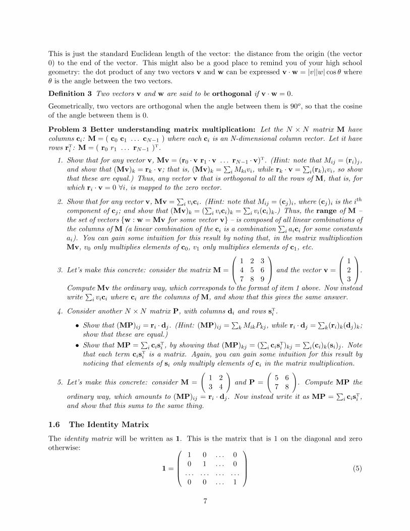
Definition 3 Two vectors v and w are said to be orthogonal if v ·w = 0.
Geometrically, two vectors are orthogonal when the angle between them is 90o, so that the cosineof the angle between them is 0.
Problem 3 Better understanding matrix multiplication: Let the N × N matrix M havecolumns ci: M = ( c0 c1 . . . cN−1 ) where each ci is an N-dimensional column vector. Let it haverows rT
i : M = ( r0 r1 . . . rN−1 )T.
1. Show that for any vector v, Mv = (r0 · v r1 · v . . . rN−1 · v)T. (Hint: note that Mij = (ri)j,and show that (Mv)k = rk · v; that is, (Mv)k =
∑iMkivi, while rk · v =
∑i(rk)ivi, so show
that these are equal.) Thus, any vector v that is orthogonal to all the rows of M, that is, forwhich ri · v = 0 ∀i, is mapped to the zero vector.
2. Show that for any vector v, Mv =∑i vici. (Hint: note that Mij = (cj)i, where (cj)i is the ith
component of cj; and show that (Mv)k = (∑i vici)k =
∑i vi(ci)k.) Thus, the range of M –
the set of vectors {w : w = Mv for some vector v} – is composed of all linear combinations ofthe columns of M (a linear combination of the ci is a combination
∑i aici for some constants
ai). You can gain some intuition for this result by noting that, in the matrix multiplicationMv, v0 only multiplies elements of c0, v1 only multiplies elements of c1, etc.
3. Let’s make this concrete: consider the matrix M =
1 2 34 5 67 8 9
and the vector v =
123
.
Compute Mv the ordinary way, which corresponds to the format of item 1 above. Now insteadwrite
∑i vici where ci are the columns of M, and show that this gives the same answer.
4. Consider another N ×N matrix P, with columns di and rows sTi .
• Show that (MP)ij = ri · dj. (Hint: (MP)ij =∑kMikPkj, while ri · dj =
∑k(ri)k(dj)k;
show that these are equal.)
• Show that MP =∑i cis
Ti , by showing that (MP)kj = (
∑i cis
Ti )kj =
∑i(ci)k(si)j. Note
that each term cisTi is a matrix. Again, you can gain some intuition for this result by
noticing that elements of si only multiply elements of ci in the matrix multiplication.
5. Let’s make this concrete: consider M =
(1 23 4
)and P =
(5 67 8
). Compute MP the
ordinary way, which amounts to (MP)ij = ri · dj. Now instead write it as MP =∑i cis
Ti ,
and show that this sums to the same thing.
1.6 The Identity Matrix
The identity matrix will be written as 1. This is the matrix that is 1 on the diagonal and zerootherwise:
1 =
1 0 . . . 00 1 . . . 0. . . . . . . . . . . .0 0 . . . 1
(5)
7

Note that 1v = v and vT1 = vT for any vector v, and 1M = M1 = M for any matrix M. (Thedimension of the matrix 1 is generally to be inferred from context; at any point, we are referring tothat identity matrix with the same dimension as the other vectors and matrices being considered).
Exercise 2 Verify that 1v = v and vT1 = vT for any vector v, and 1M = M1 = M for anymatrix M.
1.7 The Inverse of a Matrix
Definition 4 The inverse of a square matrix M is a matrix M−1 satisfying M−1M = MM−1 =1.
Fact 1 For square matrices A and B, if AB = 1, then BA = 1; so knowing either AB = 1 orBA = 1 is enough to establish that A = B−1 and B = A−1.
Not all matrices M have an inverse; but if a matrix has an inverse, that inverse is unique (thereis at most one matrix that is the inverse of M, proof for square matrices: suppose C and B areboth inverses of A. Then CAB = C(AB) = C1 = C; but also CAB = (CA)B = 1B = B; henceC = B). Intuitively, the inverse of M “undoes” whatever M does: if you apply M to a vector ormatrix, and then apply M−1 to the result, you end up having applied the identity matrix, that is,not having changed anything. If a matrix has an inverse, we say that it is invertible.
A matrix fails to have an inverse when it maps some nonzero vector(s) to the zero vector, 0.Suppose Mv = 0 for v 6= 0. Then, since matrix multiplication is a linear operation, for any othervector w, M(av + w) = aMv + Mw = Mw, so all input vectors of the form av + w are mappedto the same output vector Mw. Hence in this case the action of M cannot be undone – given theoutput vector Mw, we cannot say which input vector produced it.
You may notice that above, we defined addition, subtraction, and multiplication for matrices,but not division. Ordinary division is really multiplying by the inverse of a number: x/y = y−1xwhere y−1 = 1/y. As you might imagine, the generalization for matrices would be multiplying bythe inverse of a matrix. Since not all matrices have inverses, it turns out to be more sensible toleave it at that, and not define division as a separate operation for matrices.
Exercise 3 Suppose A and B are both invertible N ×N matrices. Show that (AB)−1 = B−1A−1.(Hint: just multiply AB times B−1A−1 and see what you get.) Similarly if C is another invertibleN ×N matrix, (ABC)−1 = C−1B−1A−1; etc. This should remind you of the result of problem 2for transposes.
Exercise 4 Show that (AT)−1 = (A−1)T. Hint: take the equation (AT)−1AT = 1, and take thetranspose.
1.8 Why Vectors and Matrices? – Two Toy Problems
As mentioned at the outset, in problems of theoretical neuroscience, we are often dealing withlarge sets of variables — the activities of a large set of neurons in a network; the development of alarge set of synaptic strengths impinging on a neuron. The equations to describe models of thesesystems are usually best expressed and analyzed in terms of vectors and matrices. Here are twosimple examples of the formulation of problems in these terms; as we go along we will develop thetools to analyze them.
8
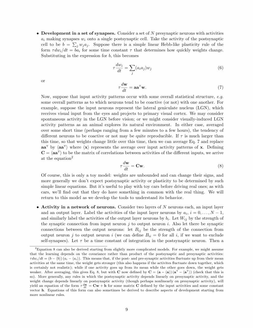
• Development in a set of synapses. Consider a set of N presynaptic neurons with activitiesai making synapses wi onto a single postsynaptic cell. Take the activity of the postsynapticcell to be b =
∑j wjaj . Suppose there is a simple linear Hebb-like plasticity rule of the
form τdwi/dt = bai for some time constant τ that determines how quickly weights change.Substituting in the expression for b, this becomes
τdwidt
=∑j
(aiaj)wj (6)
or
τdw
dt= aaTw. (7)
Now, suppose that input activity patterns occur with some overall statistical structure, e.g.some overall patterns as to which neurons tend to be coactive (or not) with one another. Forexample, suppose the input neurons represent the lateral geniculate nucleus (LGN), whichreceives visual input from the eyes and projects to primary visual cortex. We may considerspontaneous activity in the LGN before vision; or we might consider visually-induced LGNactivity patterns as an animal explores its natural environment. In either case, averagedover some short time (perhaps ranging from a few minutes to a few hours), the tendency ofdifferent neurons to be coactive or not may be quite reproducible. If τ is much larger thanthis time, so that weights change little over this time, then we can average Eq. 7 and replaceaaT by 〈aaT〉 where 〈x〉 represents the average over input activity patterns of x. DefiningC = 〈aaT〉 to be the matrix of correlations between activities of the different inputs, we arriveat the equation2
τdw
dt= Cw. (8)
Of course, this is only a toy model: weights are unbounded and can change their signs, andmore generally we don’t expect postsynaptic activity or plasticity to be determined by suchsimple linear equations. But it’s useful to play with toy cars before driving real ones; as withcars, we’ll find out that they do have something in common with the real thing. We willreturn to this model as we develop the tools to understand its behavior.
• Activity in a network of neurons. Consider two layers of N neurons each, an input layerand an output layer. Label the activities of the input layer neurons by ai, i = 0, . . . , N − 1,and similarly label the activities of the output layer neurons by bi. Let Wij by the strength ofthe synaptic connection from input neuron j to output neuron i. Also let there be synapticconnections between the output neurons: let Bij be the strength of the connection fromoutput neuron j to output neuron i (we can define Bii = 0 for all i, if we want to excludeself-synapses). Let τ be a time constant of integration in the postsynaptic neuron. Then a
2Equation 8 can also be derived starting from slightly more complicated models. For example, we might assumethat the learning depends on the covariance rather than product of the postsynaptic and presynaptic activities:τdwi/dt = (b− 〈b〉) (ai − 〈ai〉). This means that, if the post- and pre-synaptic activities fluctuate up from their meanactivities at the same time, the weight gets stronger (this also happens if the activites fluctuate down together, whichis certainly not realistic); while if one activity goes up from its mean while the other goes down, the weight getsweaker. After averaging, this gives Eq. 8, but with C now defined by C = (a− 〈a〉) (aT − 〈aT〉) (check that this isso). More generally, any rules in which the postsynaptic activity depends linearly on presynaptic activity, and theweight change depends linearly on postsynaptic activity (though perhaps nonlinearly on presynaptic activity), willyield an equation of the form τ dw
dt= Cw + h for some matrix C defined by the input activities and some constant
vector h. Equations of this form can also sometimes be derived to describe aspects of development starting frommore nonlinear rules.
9

very simple, linear model of activity in the output layer, given the activity in the input layer,would be:
τdbidt
= −bi +∑j
Wijaj +∑j
Bijbj . (9)
The −bi term on the right just says that, in the absence of input from other cells, the neuron’sactivity bi decays to zero (with time constant τ). Again, this is only a toy model, e.g. ratescan go positive or negative and are unbounded in magnitude.
Eq. 9 can be written as a vector equation:
τdb
dt= −b + Wa + Bb (10)
= −(1−B)b + Wa
Wa is a vector that is independent of b: (Wa)i =∑jWijaj is the external input to output
neuron i. So, let’s give it a name: we’ll call the vector of external inputs h = Wa. Thus, ourequation finally is
τdb
dt= −(1−B)b + h (11)
This is very similar in form to Eq. 8 for the previous model: the right side has a term inwhich the variable whose time derivative we are studying (b or w) is multiplied by a matrix(here, −(1−B); previously, C). In addition, this equation now has a term h independent ofthat variable. (In general, an equation of the form d
dtx = Cx is called homogeneous, while
one with an added constant term, ddtx = Cx + h, is called inhomogeneous.)
We can also write down an equation for the steady-state or fixed-point output activity patternbFP for a given input activity pattern h: by definition, a steady state or fixed point is a pointwhere db
dt = 0. Thus, the fixed point is determined by
(1−B)bFP = h (12)
If the matrix (1 −B) has an inverse, (1 −B)−1, then we can multiply both sides of Eq. 12by this inverse to obtain
bFP = (1−B)−1h (13)
We’ll return to this later to better understand what this equation means.
2 Coordinate Systems, Orthogonal Basis Vectors, and OrthogonalChange of Basis
To solve the equations that arise in the toy models just introduced, and in many other models, itwill be critical to be able to view the problem in alternative coordinate systems. Choice of the rightcoordinate system will greatly simplify the equations and allow us to solve them. So, in this sectionwe address the topic of coordinate systems: what they are, what it means to change coordinates,and how we change them. We begin by addressing the problem in two dimensions, where one candraw pictures and things are more intuitively clear. We’ll then generalize our results to higherdimensions, as needed to address problems involving many variables such as our toy models. Fornow we are only going to consider coordinate systems in which each coordinate axis is orthogonalto all the other coordinate axes; much later we will consider more general coordinate systems.
10
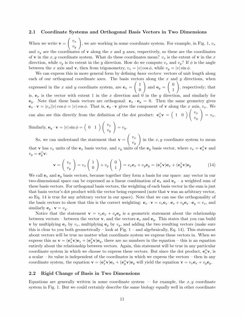
2.1 Coordinate Systems and Orthogonal Basis Vectors in Two Dimensions
When we write v =
(vxvy
), we are working in some coordinate system. For example, in Fig. 1, vx
and vy are the coordinates of v along the x and y axes, respectively, so these are the coordinatesof v in the x, y coordinate system. What do these coordinates mean? vx is the extent of v in the xdirection, while vy is its extent in the y direction. How do we compute vx and vy? If φ is the anglebetween the x axis and v, then from trigonometry, vx = |v| cosφ, while vy = |v| sinφ.
We can express this in more general form by defining basis vectors: vectors of unit length alongeach of our orthogonal coordinate axes. The basis vectors along the x and y directions, when
expressed in the x and y coordinate system, are ex =
(10
)and ey =
(01
), respectively; that
is, ex is the vector with extent 1 in the x direction and 0 in the y direction, and similarly forey. Note that these basis vectors are orthogonal: ex · ey = 0. Then the same geometry givesex · v = |ex||v| cosφ = |v| cosφ. That is, ex · v gives the component of v along the x axis, vx. We
can also see this directly from the definition of the dot product: eTxv =
(1 0
)( vxvy
)= vx.
Similarly, ey · v = |v| sinφ =(
0 1)( vx
vy
)= vy.
So, we can understand the statement that v =
(vxvy
)in the x, y coordinate system to mean
that v has vx units of the ex basis vector, and vy units of the ey basis vector, where vx = eTxv and
vy = eTyv:
v =
(vxvy
)= vx
(10
)+ vy
(01
)= vxex + vyey = (eT
xv)ex + (eTyv)ey (14)
We call ex and ey basis vectors, because together they form a basis for our space: any vector in ourtwo-dimensional space can be expressed as a linear combination of ex and ey – a weighted sum ofthese basis vectors. For orthogonal basis vectors, the weighting of each basis vector in the sum is justthat basis vector’s dot product with the vector being expressed (note that v was an arbitrary vector,so Eq. 14 is true for any arbitrary vector in our space). Note that we can use the orthogonality ofthe basis vectors to show that this is the correct weighting: ex · v = vxex · ex + vyex · ey = vx, andsimilarly ey · v = vy.
Notice that the statement v = vxex + vyey is a geometric statement about the relationshipbetween vectors – between the vector v, and the vectors ex and ey. This states that you can buildv by multiplying ex by vx, multiplying ey by vy, and adding the two resulting vectors (make surethis is clear to you both geometrically – look at Fig. 1 – and algebraically, Eq. 14). This statementabout vectors will be true no matter what coordinate system we express these vectors in. When weexpress this as v = (eT
xv)ex + (eTyv)ey, there are no numbers in the equation – this is an equation
entirely about the relationship between vectors. Again, this statement will be true in any particularcoordinate system in which we choose to express these vectors. But since the dot product, eT
xv, isa scalar – its value is independent of the coordinates in which we express the vectors – then in anycoordinate system, the equation v = (eT
xv)ex + (eTyv)ey will yield the equation v = vxex + vyey.
2.2 Rigid Change of Basis in Two Dimensions
Equations are generally written in some coordinate system — for example, the x, y coordinatesystem in Fig. 1. But we could certainly describe the same biology equally well in other coordinate
11
X’Y’
O_
v
Y
Xvx
vy
vx’vy’
O_
Figure 1: Representation of a vector in two coordinate systemsThe vector v is shown represented in two coordinate systems. The (x′, y′) coordinate system is rotated byan angle θ from the (x, y) coordinate system. The coordinates of v in a given coordinate system are givenby the perpendicular projections of v onto the coordinate axes, as illustrated by the dashed lines. Thus, inthe (x, y) basis, v has coordinates (vx, vy), while in the (x′, y′) basis, it has coordinates (vx′ , vy′).
12
systems. Suppose we want to describe things in the new coordinate axes, x′, y′, determined by arigid rotation by an angle θ from the x, y coordinate axes, Fig. 1. How do we define coordinates inthis new coordinate system?
Let’s first define basis vectors ex′ , ey′ to be the vectors of unit length along the x′ and y′ axes,respectively. Like any other vectors, we can write these vectors as linear combinations of ex andey:
ex′ = (eTxex′)ex + (eT
yex′)ey (15)
ey′ = (eTxey′)ex + (eT
yey′)ey (16)
From the geometry, and the fact that the basis vectors have unit length, we find the following dotproducts:
eTxex′ = cos θ (17)
eTyex′ = sin θ (18)
eTxey′ = − sin θ (19)
eTyey′ = cos θ (20)
Thus, we can write our new basis vectors as
ex′ = cos θex + sin θey (21)
ey′ = − sin θex + cos θey (22)
(Check, from the geometry of Fig. 1, that this makes sense.)
Exercise 5 Using the expressions for ex′ and ey′ in Eqs. 21-22, check that ex′ and ey′ are orthog-onal to one another – that is, that eT
x′ey′ = 0 – and that they each have unit length – that is, thateTx′ex′ = eT
y′ey′ = 1.
Problem 4 We’ve seen that, in a given coordinate system with basis vectors e0, e1, any vector v
has the representation v =
(eT0v
eT1v
), which is just shorthand for v = (eT
0v)e0 + (eT1v)e1. Based
on this and Eqs. 21-22, we know that, in the x, y coordinate system, ex′ =
(cos θsin θ
), ey′ =(
− sin θcos θ
), ex =
(10
), ey =
(01
).
Now, show that, in the x′, y′ coordinate system, ex′ =
(10
), ey′ =
(01
), ex =
(cos θ− sin θ
),
ey =
(sin θcos θ
). (Note, for each of these four vectors v, you just have to form
(eTx′v
eTy′v
).) You can
compute the necessary dot products using the representations in the x, y coordinate system, sincedot products are coordinate-independent (although you can also just look them up from Eqs. 17-20).Note also that these equations should make intuitive sense: the x, y coordinate system is rotated by−θ from the x′, y′ system, so expressing ex, ey in terms of ex′ , ey′ should look exactly like expressingex′ , ey′ in terms of ex, ey, except that we must substitute −θ for θ; and note that cos(−θ) = cos(θ),sin(−θ) = − sin(θ).)
13

We can reexpress the above equations for each set of basis vectors in the other’s coordinatesystem in the coordinate-independent form:
ex′ = cos θex + sin θey (23)
ey′ = − sin θex + cos θey (24)
ex = cos θex′ − sin θey′ (25)
ey = sin θex′ + cos θey′ (26)
Now, verify these equations in each coordinate system. That is, first, using the x, y representation,substitute the coordinates of each vector and show that each equation is true. Then do the same thingagain using the x′, y′ representation. The numbers change, but the equations, which are statementsabout geometry that are true in any coordinate system, remain true.
OK, back to our original problem: we want to find the representation
(vx′
vy′
)of v in the new
coordinate system. As we’ve seen, this is really just a short way of saying that v = vx′ex′ + vy′ey′
where vx′ = eTx′v and vy′ = eT
y′v. But we also know that v = vxex + vyey. So, using Eqs. 17-20,we’re ready to compute:
vx′ = eTx′v = eT
x′(vxex + vyey) = vx(eTx′ex) + vy(e
Tx′ey) = vx cos θ + vy sin θ (27)
vy′ = eTy′v = eT
y′(vxex + vyey) = vx(eTy′ex) + vy(e
Ty′ey) = −vx sin θ + vy cos θ (28)
or in matrix form(vx′
vy′
)=
(eTx′ex eT
x′eyeTy′ex eT
y′ey
)(vxvy
)=
(cos θ sin θ− sin θ cos θ
)(vxvy
)(29)
Note that the first row of the matrix is just eTx′ as expressed in the ex, ey coordinate system, and
similarly the second row is just eTy′ as expressed in the ex, ey coordinate system. This should make
intuitive sense: to find vx′ , we want to find eTx′v, which is obtained by applying the first row of the
matrix to v as written in the ex, ey coordinate system; and similarly vy′ is found as eTy′v, which is
just the second row of the matrix applied to v, all carried out in the ex, ey coordinate system.
We can give a name to the above matrix: Rθ =
(cos θ sin θ− sin θ cos θ
). This is a commonly
encountered matrix known as a “rotation matrix”. Rθ represents rotation of coordinates by anangle θ: it is the matrix that transforms coordinates to a new set of coordinate axes rotated by θfrom the previous coordinate axes.
Problem 5 Verify the equation v = vxex+vyey in the x′, y′ coordinate system. That is, substitutethe x′, y′ coordinate representation of v (from Eq. 29), ex, and ey, and verify that this equationis true. It’s not quite as obvious as it was when it was expressed in the x, y coordinate system(Eq. 14), but it’s still just as true.
Problem 6 Show that RTθRθ = RθR
Tθ = 1, that is, that RT
θ = R−1θ . (Note that this makesintuitive sense, because RT
θ = R−θ; this follows from cos (−θ) = cos θ, sin (−θ) = − sin θ).
To summarize, we’ve learned how a vector v transforms under a rigid change of basis, in whichour coordinate axes are rotated counterclockwise by an angle θ. If v′ is the representation of v in
14

the new coordinate system, then v′ = Rθv. Furthermore, using the fact that RTθRθ = 1, we can
also find the inverse transform: RTθv′ = RT
θRθv = v, i.e. v = RTθv′.
Now, we face a final question: how should matrices be transformed under this change of basis?For any matrix M, let M′ be its representation in the rotated coordinate system. To see how thisshould be transformed, note that Mv is a vector for any vector v; so we know that (Mv)′ = RθMv.But the transformation of the vector Mv should be the same as the vector we get from operatingon the transformed vector v′ with the transformed matrix M′; that is, (Mv)′ = M′v′. And weknow v′ = Rθv. So, we find that M′Rθv = RθMv, for every vector v. But this can only true ifM′Rθ and RθM are the same matrix3: M′Rθ = RθM. Finally, multiplying on the right by RT
θ ,and using RθR
Tθ = 1, we find
M′ = RθMRTθ (30)
Intuitively, you can think of this as follows: to compute M′v′, which is just Mv in the newcoordinate system, you first multiply v′ by RT
θ , the inverse of Rθ. This takes v′ back to v, i.e.moves us back from the new coordinate system to the old coordinate system. You then apply Mto v in the old coordinate system. Finally, you apply Rθ to the result, to transform the result backinto the new coordinate system.
2.3 Rigid Change of Basis in Arbitrary Dimensions
As our toy models should make clear, in neural modeling we are generally dealing with vectors oflarge dimensions. The above results in two dimensions generalize nicely to N dimensions. Supposewe want to consider only changes of basis consisting of rigid rotations. How shall we define these?We define these as the class of transformations O that preserve all inner products: that is, thetransformations O such that, for any vectors v and x, v · x = (Ov) · (Ox). Transformationssatisfying this are called orthogonal transformations.
Why are these rigid? The dot product of two vectors of unit length gives the cosine of the anglebetween them, in any dimensions; and the dot product of a vector with itself tells you its length(squared). So, a dot-product-preserving transformation preserves the angles between all pairs ofvectors and the lengths of all vectors. This coincides with what we mean by a rigid rotation — nostretching, no shrinking, no distortions.
We can rewrite the dot product, (Ov) · (Ox) = (Ov)T(Ox) = vTOTOx. The requirement thatthis be equal to vTx for any vectors v and x can only be satisfied if OTO = 1.
Thus, we define:
Definition 5 An orthogonal matrix is a matrix O satisfying OTO = OOT = 1.
Note that the rotation matrix Rθ in two dimensions is an example of an orthogonal matrix. Un-der an orthogonal transformation O, a column vector is transformed v 7→ Ov; a row vector istransformed vT 7→ vTOT (as can be seen by considering (v)T 7→ (Ov)T = vTOT); and a matrix istransformed M 7→ OMOT.
The argument as to why M is mapped to OMOT is just as we worked out for two dimensions;the argument goes through unchanged for arbitrary dimensions. Here are two other ways to see it:
• The outer product vxT is a matrix. Under an orthogonal change of basis, v 7→ Ov, x 7→ Ox,so the outer product is mapped vxT 7→ (Ov)(Ox)T = OvxTOT = O(vxT)OT. Thus, thematrix vxT transforms as indicated.
3Given that Av = Bv for all vectors v, suppose the ith column of A is not identical to the ith column of B. Thenchoose v to be the vector that is all 0’s except a 1 in the ith position. Then Av is just the ith column of A, andsimilarly for Bv, so Av 6= Bv for this vector. Contradiction. Therefore every column of A and B must be identical,i.e. A and B must be identical.
15
• An expression of the form vTMx is a scalar, so it is unchanged by a coordinate transfor-mation. In the new coordinates, this is (Ov)TM̃Ox, where M̃ is the represention of M inthe new coordinate system. Thus, (Ov)TM̃Ox = vTMx, for any v, x, and M and orthog-onal transform O. We can rewrite vTMx by inserting the identity, 1 = OTO, as follows:vTMx = vT1M1x = vT(OTO)M(OTO)x = (Ov)T(OMOT)Ox. The only way this can beequal to (Ov)TM̃Ox for any v and x is if M̃ = (OMOT).
Exercise 6 Show that the property “M is the identity matrix” is basis-independent, that is, O1OT =1. Thus, the identity matrix looks the same in any basis.
Exercise 7 Note that the property “x is the zero vector” (x = 0; x is the vector all of whoseelements are zero) is basis-independent; that is, if x = 0, then Ox = 0 for any O. Similarly, “Mis the zero matrix” (M = 0; M is the matrix all of whose elements are zero) is basis-independent:if M = 0, then OMOT = 0 for any O.
Problem 7 1. Show that the property “P is the inverse of M” is basis-independent. That is, ifP = M−1, then OPOT = (OMOT)−1, where O is orthogonal. (Hint: to show that A = B−1,just show that AB = 1.)
2. Note, from problem 2, that (OMOT)T = OMTOT. Use this result to prove two immediatecorollaries:
• The property “P is the transpose of M” is invariant under orthogonal changes of basis:that is, OPOT = (OMOT)T for P = MT.
• The property “M is symmetric” is invariant under orthogonal changes of basis: that is,if M = MT, (OMOT)T = OMOT.
Problem 8 Write down arguments to show that (1) a dot-product preserving transformation isone for which OTO = 1; and (2) under this transformation, M 7→ OMOT — without looking atthese notes. You can look at these notes as much as you want in preliminary tries, but the last tryyou have to go from beginning to end without looking at the notes.
2.4 Complete Orthonormal Bases
Consider the standard basis vectors in N dimensions: e0 = (1, 0, . . . , 0)T, e1 = (0, 1, . . . , 0)T, . . .,eN−1 = (0, 0, . . . , 1)T. These form an orthonormal basis. This means: (1) The ei are mutuallyorthogonal: eT
i ej = 0 for i 6= j; and (2) the ei are each normalized to length 1: eTi ei = 1,
i = 0, . . . , N − 1. We can summarize and generalize this by use of the Kronecker delta:
Definition 6 The Kronecker delta δij is defined by δij = 1, i = j; δij = 0, i 6= j.
Note that δij describes the elements of the identity matrix: (1)ij = δij .
Problem 9 Show that, for any vector x,∑j δijxj = xi. This ability of the Kronecker delta to
“collapse” a sum to a single term is something that will be used over and over again. Note thatthis equation is just the equation 1x = x, in component form.
Definition 7 A set of N vectors ei, i = 0, . . . , N − 1, form an orthonormal basis for an N-dimensional vector space if eT
i ej = δij.
16

Exercise 8 Show that in two dimensions, the vectors e0 = R(θ)(1, 0)T = (cos θ,− sin θ)T, ande1 = R(θ)(0, 1)T = (sin θ, cos θ)T, form an orthonormal basis, for any angle θ.
Exercise 9 Prove that an orthonormal basis remains an orthonormal basis after transformationby an orthogonal matrix. Your proof is likely to consist of writing down one sentence about whatorthogonal transforms preserve.
Let’s restate more generally what we learned in two dimensions: when we state that v =(v0, v1, . . . , vN−1)
T in some orthonormal basis ei, we mean that v has extent v0 in the e0 direction,etc. We can state this more formally by writing
v = v0e0 + . . .+ vN−1eN−1 =∑i
viei (31)
This is an expansion of the vector v in the ei basis: an expression of v as a weighted sum of theei. This is, in essence, what it means for the ei to be a basis: any vector v can be written as aweighted sum of the ei. The coefficients of the expansion, vi, are the components of v in the basisof the ei; we summarize all of this when we state that v = (v0, v1, . . . , vN−1)
T in the ei basis. Thecoefficients vi are given by the dot product of v and ei: vi = eT
i v:
Problem 10 Show that vj = eTj v. (Hint: multiply Eq. 31 from the left by eT
j , and use the resultof Problem 9.)
In particular, we can expand the basis vectors in themselves:
ei = (eT0ei)e0 + . . .+ (eT
N−1ei)eN−1 =∑j
(eTj ei)ej =
∑j
δijej = ei. (32)
That is, the basis vectors, when expressed in their own basis, are always just written e0 =(1, 0, . . . , 0)T, e1 = (0, 1, . . . , 0)T, . . ., eN−1 = (0, 0, . . . , 1)T. Thus, the equation v =
∑i viei
(Eq. 31), when written in the ei basis, just represents the intuitive statement
v =
v0v1. . .vN−1
= v0
10. . .0
+ v1
01. . .0
+ . . .+ vN−1
00. . .1
=∑i
viei (33)
In summary, for any vector v and orthonormal basis ei, we can write
v =∑i
ei(eTi v) =
∑i
viei (34)
In particular, any orthonormal basis vectors ei, when expressed in their own basis, have the simplerepresentation e0 = (1, 0, . . . , 0)T, e1 = (0, 1, . . . , 0)T, . . ., eN−1 = (0, 0, . . . , 1)T.
We can rewrite v =∑i ei(e
Ti v) as v =
∑i(eie
Ti )v = (
∑i eie
Ti )v. Since this is true for any
vector v, this means that∑i eie
Ti = 1, the identity matrix. This is true for any orthonormal basis.
Problem 11 For any orthonormal basis ei, i = 0, . . . , N − 1: Show that∑i eie
Ti = 1, by working
in the ei basis, as follows. In that basis, show that eieTi is the matrix composed of all 0’s, except
for a 1 on the diagonal in the ith row/column. Do the summation to show that∑i eie
Ti = 1.
17

Exercise 10 Make sure you understand the following. Although you have derived∑i eie
Ti = 1 in
Problem 11 by working in a particular basis, the result is general: it is true no matter in whichorthonormal basis you express the ei. This follows immediately from exercise 6. Or, you can seethis explicitly, for example, by transforming the equation to another orthonormal basis by applyingan orthogonal matrix O on the left and OT on the right. This gives
∑i Oeie
Ti O
T = O1OT, whichbecomes
∑i(Oei)(Oei)
T = 1. Thus, the equation holds for the ei as expressed in the new coordinatesystem.
We can restate the fact that∑i eie
Ti = 1 in words to, hopefully, make things more intuitive,
as follows. The matrix eieTi , when applied to the vector v, finds the component of v along the ei
direction, and multiplies this by the vector ei: (eieTi )v = ei(e
Ti v) = viei. That is, eie
Ti finds the
projection of v along the ei axis. When the ei form an orthonormal basis, these separate projectionsare independent: any v is just the sum of its projections onto each of the ei: v =
∑i ei(e
Ti v). Taking
the projections of v onto each axis of a complete orthonormal basis, and adding up the results,just reconstitutes the vector v. (For example, Fig. 1 illustrates that in two dimensions, adding thevectors vxex and vyey, the projections of v on the x and y axes, reconstitutes v.) That is, theoperation of taking the projections of v on each axis, and then summing the projections, is justthe identity operation; so
∑i eie
Ti = 1.
The property∑i eie
Ti = 1 represents a pithy summation of the fact that an orthonormal basis
is complete:
Definition 8 A complete basis for a vector space is a set of vectors ei such that any vector vcan be uniquely expanded as a weighted sum of the ei: v =
∑i viei, where there is only one set of
vi for a given v that will satisfy this equation.
Fact 2 An orthonormal set of vectors ei forms a complete basis if and only if∑i eie
Ti = 1.
Intuitively: if we have an incomplete basis – we are missing some directions – then∑i eie
Ti will give
0 when applied to vectors representing the missing directions, so it can’t be the identity; saying∑i eie
Ti = 1 means that it reconstitutes any vector, so there are no missing directions.
More formally, we can prove this as follows: if∑i eie
Ti = 1, then for any vector v, v = 1v =∑
i eieTi v =
∑i viei where vi = eT
i v. So any vector v can be represented as a linear combinationof the ei, so they form a complete basis. Conversely, if the ei form a complete basis, then for anyvector v, v =
∑i viei for some vi. By the orthonormality of the ei, taking the dot product with
ej gives ej · v =∑i viej · ei =
∑i viδji = vj . So for any v, v =
∑i eivi =
∑i eie
Ti v = (
∑i eie
Ti ) v.
This can only be true for every vector v if∑i eie
Ti = 1.
Fact 3 In an N-dimensional vector space, a set of orthonormal vectors forms a complete basis ifand only if the set contains N vectors.
That is, any set of N orthonormal vectors constitutes a complete basis; you can’t have more thanN mutually orthonormal vectors in an N-dimensional space; and if you only have N-1 (or fewer)orthonormal vectors, you’re missing a direction and so can’t represent vectors pointing in thatdirection or that have a component in that direction.
Finally, we’ve interpreted the components of a vector, v = (v0, v1, . . . , vN−1)T, as describing v
only in some particular basis; the more general statements, given some underlying basis vectorsei, are v =
∑i viei, where vi = eT
i v. We now do the same for a matrix. We write M = 1M1 =
18

(∑i eie
Ti )M(
∑j eje
Tj ) =
∑i,j ei(e
Ti Mej)e
Tj . But (eT
i Mej) is a scalar; call it Mij . Since a scalarcommutes with anything, we can pull this out front; thus, we have obtained
M =∑ij
MijeieTj where Mij = eT
i Mej (35)
When working in the basis of the ei vectors, eieTj is the matrix that is all 0’s except for a 1 in the
ith row, jth column (verify this!). Thus, in the basis of the ei vectors,
M =
M00 M01 . . . M0(N−1)M10 M11 . . . M1(N−1). . . . . . . . . . . .
M(N−1)0 M(N−1)1 . . . M(N−1)(N−1)
(36)
Thus, the Mij = eTi Mej are the elements of M in the ei basis, just as vi = eT
i v are the elementsof v in the ei basis. The more general description of M is given by Eq. 35.
2.5 Which Basis Does an Orthogonal Matrix Map To?
Suppose we change basis by some orthogonal matrix O: v 7→ Ov, M 7→ OMOT. What basis arewe mapping to? The answer is: in our current basis, O is the matrix each of whose rows is one ofthe new basis vectors, as expressed in our current basis. This should be intuitive: applying the firstrow of O to a vector v, we should get the coordinate of v along the first new basis vector e0; but thiscoordinate is eT
0v, hence the first row should be eT0 . We can write this as O = ( e0 e1 . . . eN−1 )T,
where e0 means a column of our matrix corresponding to the new basis vector e0 as expressed inour current basis. To be precise, we mean the following: letting (O)ij be the (ij)th component ofthe matrix O, and letting (ei)j be the jth component of new basis vector ei (all of these componentsexpressed in our current basis), then (O)ij = (ei)j . It of course follows that each column of OT isone of the new basis vectors, that is, OT = ( e0 e1 . . . eN−1 ).
Problem 12 Use the results of problem 3, or rederive from scratch, to show the following:
1. Show that the statement OOT = 1 simply states the orthonormality of the new basis vectors:eTi ej = δij.
2. Similarly, show that the statement OTO = 1 simply expresses the completeness of the newbasis vectors:
∑i eie
Ti = 1.
2.6 Recapitulation: The Transformation From One Orthogonal Basis To An-other
We have seen that, for any orthonormal basis {ei}, any vector v can be expressed v =∑i viei where
vi = eTi v, and any matrix M can be expressed M =
∑ijMijeie
Tj where Mij = eT
i Mej . Consideranother orthonormal basis {fi}. Using 1 =
∑k fkf
Tk , we can derive the rules for transforming
coordinates from the {ei} basis to the {fi} basis, and in so doing recapitulate the results of thischapter, as follows:
• Transformation of a vector: write v =∑i viei =
∑i vi1ei =
∑ik vifkf
Tk ei =
∑k v′kfk, where
v′k =∑i f
Tk eivi =
∑iOkivi, and the matrix O is defined by Oki = fT
k ei. That is, thecoordinates v′i of v in the {fk} coordinate system are given, in terms of the coordinates vi inthe {ei} coordinate system, by v′ = Ov.
19

Note that O is indeed orthogonal: (OOT)ij =∑k OikOjk =
∑k fTi ekf
Tj ek =
∑k fTi eke
Tk fj =
fTi (∑k eke
Tk )fj = fT
i fj = δij ; while (OTO)ij =∑k OkiOkj =
∑k fTk eif
Tk ej =
∑k eT
i fkfTk ej =
eTi (∑k fkf
Tk )ej = eT
i ej = δij .
Note also that the ith row of O has elements Oij = fTi ej , with j varying across the row; these
are just the coordinates of fi in the {ej} basis – that is, the ith row of O is precisely thevector fT
i as expressed in the {ej} basis. The ith column of O has elements Oji = fTj ei, with j
varying across the column – these are the coordinates of ei in the fj basis. So the ith columnis just the ith old basis vector, written in the coordinates of the new basis, while the ith rowis the ith new basis vector, written in the coordinates of the old basis. Thus, when we takethe transpose of O, the roles of the two basis sets are reversed; so OT is the mapping fromthe {fi} basis to the {ei} basis, and thus is the inverse of O.
• Transformation of a matrix: write M =∑ijMijeie
Tj =
∑ijMij1eie
Tj 1 =
∑ijklMijfkf
Tk eie
Tj flf
Tl =∑
klM′klfkf
Tl where M ′kl =
∑ij f
Tk eiMije
Tj fl =
∑ij OkiMijOlj =
∑ij OkiMijO
Tjl, where again
the matrix O is defined by Oij = fTi ej . That is, the coordinates M ′ij of M in the {fi} coor-
dinate system are given, in terms of the coordinates Mij in the {ei} coordinate system, byM′ = OMOT.
2.7 Summary
Vectors and matrices are geometrical objects. The vector v has some length and points in somedirection in the world, independent of any basis. Similarly, a given matrix represents the sametransformation – for example, the one that takes ex′ to ex and ey′ to ey in Fig. 1 – in any basis.
To talk about vectors and matrices, we generally define some complete orthonormal basis. Thisis a set of N vectors ei, where N is the dimension of the space, that satisfy eT
i ej = δij . The fact thatthe basis is complete means that any vector can be written as a weighted sum of these basis vectors:v =
∑i viei where vi = eT
i v. This completeness is summarized by the fact that∑i eie
Ti = 1, where
1 is the identity matrix.The choice of basis is, in principal, arbitrary. Transformations between orthonormal bases are
given by orthogonal transformations, determined by matrices O satisfying OOT = OTO = 1.Vectors transform as v 7→ Ov, while matrices transform as M 7→ OMOT. The rows of O are thenew basis vectors, as written in the coordinate system of the current basis vectors.
The interesting properties of vectors and matrices are those that are geometric, that is, indepen-dent of basis. Any scalars formed from vector and matrix operations are invariant under orthogonalchanges of basis, for example the dot product xTy of any two vectors x and y, or the quantityxTMy for any two vectors x and y and matrix M (note that the latter is just a dot product of twovectors, xT(My). From this follows the orthogonal-basis-independence of such geometric quantitiesas the length |v| of a vector v (|v| =
√vTv) or the angle θ between two vectors x and y (which
is the inverse cosine of xTy/|x||y| = cos θ). Similarly, equalities between vectors or matrices arebasis-independent: e.g., if Mv = y in one basis, the same is true in any basis. Thus, a matrix Mrepresents the same transformation in any basis – it takes the same vectors v to the same vectors y.A number of other properties are also preserved under orthogonal transformations, such as whetheror not a set of vectors is orthonormal (this follows from the preservations of length and angles),whether or not a matrix is symmetric, and whether or not a matrix is orthogonal.
In the next section, we will see that both the familiarity we have gained with vectors andmatrices, and in particular the freedom we have developed to switch between bases, will help us togreatly simplify and solve linear differential equations, such as those that arise in studying simplemodels of neural activity and synaptic development.
20
3 Linear Differential Equations, Eigenvectors and Eigenvalues
The formulation of our toy models led us to linear differential equations of the form ddtv = Mv+h.
Here v is the vector whose time evolution we are studying, like the vector of weights in our modelof synaptic development, or the vector of neural activities in our model of activity in a circuit;M is a matrix; and h is a constant vector. An equation of this form is called an inhomogeneousequation; an equation of the form d
dtv = Mv is a homogeneous equation. We will focus on thehomogeneous equation, because once we understand how to solve this, solving the inhomogeneouscase is easy. At the end of this section, we’ll return to the inhomogeneous case and show how it’ssolved. Solving d
dtv = Mv is easy if we can find the eigenvectors and eigenvalues of the matrixM, so much of this section will be devoted to understanding what these are. But we’ll begin, onceagain, by thinking about the problem in one or two dimensions.
3.1 Linear Differential Equations in Vector Form
The solution to the simple linear differential equation,
d
dtv = kv (37)
isv(t) = v(0)ekt (38)
where v(0) is the value of v at t = 0.
Exercise 11 If this is not obvious to you, show that Eq. 38 is indeed a solution to Eq. 37.
Now, consider two independent equations:
d
dtv0 = k0v0 (39)
d
dtv1 = k1v1 (40)
We can rewrite these as the matrix equation
d
dtv = Mv (41)
where v =
(v0v1
)and M =
(k0 00 k1
). That is:
d
dt
(v0v1
)=
(k0 00 k1
)(v0v1
). (42)
Exercise 12 Satisfy yourself that Eq. 42 is, component-wise, identical to Eqs. 39-40.
Of course, Eq. 42 has the solution
v0(t) = v0(0)ek0t (43)
v1(t) = v1(0)ek1t (44)
Congratulations!! You’ve just solved your first matrix differential equation. Pretty easy, eh?
21
Moral 1 When a matrix M is diagonal (that is, has nonzero entries only along the diagonal), theequation d
dtv = Mv is trivial — it is just a set of independent, one-dimensional equations.
Exercise 13 Let’s clarify the meaning of Eqs. 41-42. What does it mean to take the time derivativeof a vector, d
dtv? First, it means that v is a vector function of time, v(t) (but we generally won’texplicitly write the ‘(t)’); that is, v represents a different vector at each time t. The equationddtv = Mv tells the vector change in v(t) in a short time ∆t: v(t + ∆t) = v(t) + Mv(t)∆t.Now, expand v =
∑i viei in some basis ei. Note that the ei are fixed, time-invariant vectors:
ddtei = 0. The time-dependence of v is reflected in the time-dependence of the vi. Thus, we can
write ddtv = d
dt (∑i viei) =
∑i ei
ddtvi. In the ei basis,
∑i ei
ddtvi =
(ddtv0ddtv1
)= d
dt
(v0v1
).
Now, suppose you’ve been given the set of two independent equations in Eqs. 39–42; butyou’ve been given them in the wrong coordinate system. This could happen if somebody didn’tknow anything about v0 and v1, and instead measured things in some different coordinates thatseemed natural from the viewpoint of an experiment. We’re going to find that that’s exactly thecase in our toy models: in the coordinates in which we’re given the problem – the weights, or theactivities – the relevant matrix is not diagonal; but there is a coordinate system in which the matrixis diagonal. So, let’s say the coordinates that were measured turn out to be w0 = (v0 + v1)/
√2,
w1 = (−v0+v1)/√
2. (The factors of√
2 are included to make this an orthogonal – length-preserving– change of coordinates.) We can express this as a matrix equation:(
w0
w1
)=
1√2
(1 1−1 1
)(v0v1
). (45)
We could also find this transformation matrix by thinking geometrically about the change of basisinvolved in going from v to w. It’s not hard to see (draw a picture of v and w! – for example, setv along the x axis, and work in x, y coordinates) that this represents a rotation of coordinates by45◦ = π/4. That is, our transformation matrix is
Rπ/4 =
(cosπ/4 sinπ/4− sinπ/4 cosπ/4
)=
1√2
(1 1−1 1
)(46)
Thus, the equation ddtv = Mv will be transformed into d
dt(Rπ/4v) = (Rπ/4MRT
π/4)(Rπ/4v), or
d
dtw = M̃w (47)
where
w = Rπ/4v, M̃ = Rπ/4MRT
π/4 =1
2
(k1 + k0 k1 − k0k1 − k0 k1 + k0
)(48)
In components, this is
d
dt
(w0
w1
)=
1
2
(k1 + k0 k1 − k0k1 − k0 k1 + k0
)(w0
w1
)(49)
Problem 13 • Show that the elements of Rπ/4MRT
π/4 are as given in Eq. 48.
• Show that the equation ddtv = Mv, after multiplying both sides from the left by Rπ/4, trans-
forms into the equation ddtw = M̃w. Note, to achieve this, you can insert 1 = RT
π/4Rπ/4
between M and v.
22

LEFT RIGHT
w0
w1
Figure 2: A Very Simple Model of Ocular DominanceTwo input cells, one from each eye, project to one output cell. The synapse from the left-eye cell is w0; thatfrom the right-eye cell is w1.
So, we have a messy-looking matrix equation for w. The developments of w0 and w1 are coupled:the development of w0 depends on both w0 and w1, and similarly for the development of w1. Butwe know that really, there are two independent, uncoupled one-dimensional equations hidden here:the development of v0 depends only on v0, that of v1 only on v1. Things are really simple, if we canonly find our way back. How do we find our way back, assuming we don’t know the transformationthat got us here in the first place? That is, given Eq. 49, how could we ever realize that, by achange of basis, we could change it into Eq. 42, where the matrix is diagonal and the equationstrivial?
The answer is, we have to find the eigenvectors of the matrix M̃ , as explained in the followingsections. This is a general method for finding the coordinates (if any exist — more on that in a bit)in which the matrix determining time development becomes diagonal. In this coordinate system,the equations become trivial — just a set of independent, uncoupled, one-dimensional equations.
Before considering how to do that in general, however, let’s consider our example problemsagain.
3.2 Two Examples
3.2.1 A Simple Correlation-Based Model of Ocular Dominance
We consider perhaps the simplest possible model of ocular dominance: one postsynaptic cell, twopresynaptic cells, one from each eye. There are two synapses, one from each presynaptic cell ontothe postsynaptic cell. Let the synaptic strength from the left eye be w0, that from the right eye,w1 (Fig. 2).
Assume we have a correlation-based rule for synaptic development of the form τ ddtwi =
∑j Cijwj ,
where C is the matrix of correlations between the inputs, and τ is a constant determining the speedof development (Eq. 8). Let the self-correlation be 1, and let the between-eye correlation be ε. Thenthe synaptic development equations are
τd
dtw0 = (w0 + εw1) (50)
23

τd
dtw1 = (εw0 + w1) (51)
or, in matrix notation,
τd
dtw = Cw (52)
where the correlation matrix is
C =
(1 εε 1
)(53)
Exercise 14 Make sure you understand exactly where every term in Eqs. 50-53 comes from.
Eq. 52 has exactly the same form as Eq. 47. The equations are identical if we set 1τC = M̃;
this requires (k1 + k0)/2 = 1/τ , (k1 − k0)/2 = ε/τ , which we can solve to find k0 = (1 − ε)/τ ,k1 = (1 + ε)/τ . Thus, with this identification, Eq. 52 is Eq. 47.
Exercise 15 Don’t just take my word for it: show that the equations are equivalent when k0 andk1 are as stated.
In this case, the natural experimental variables were the synaptic weights — w0 and w1. But,by the derivation of Eq. 47 from Eq. 42, we know that the variables in which the equations simplify— in which they become independent, one-dimensional equations — are v0 = (1/
√2)(w0 − w1),
and v1 = (1/√
2)(w0 + w1). These correspond, respectively, to the ocular dominance or differencebetween the strength of the two eyes, v0, and the sum of the two eyes’ strength, v1. We know thesolutions to this model: from Eqs. 43-44, they are
v0(t) = v0(0)e(1−ε)τ
t (54)
v1(t) = v1(0)e(1+ε)τ
t (55)
So, when the two eyes are anticorrelated — when ε < 0 — then the ocular dominance v0 outgrowsthe sum of the two eyes’ strengths v1. But when the two eyes are correlated — when ε > 0 — thenthe sum outgrows the ocular dominance. In either case, the sum and the ocular dominance growindependently – each grows along its merry way, oblivious to the presence of the other.
Problem 14 Show that, when the ocular dominance v0 outgrows the sum v1, the eye whose synapticstrength is initially strongest takes over — its synapse grows, and the other eye’s synapse shrinks(or grows more negative). Show that when the sum v1 outgrows the ocular dominance v0, botheyes’ synapses grow (although the difference between their strengths — the ocular dominance —also grows, for ε < 1).
To show these results, note that (1) the left eye’s synaptic strength w0, is proportional to v1+v0,while the right eye’s strength w1 is proportional to v1 − v0; (2) if the left eye’s synapse is initiallystronger, v0(0) > 0 and v0 grows increasingly more positive with time; while if the right eye’ssynapse is initially stronger, v0(0) < 0 and v0 grows increasingly more negative with time.
Note that we have not incorporated anything in this model to make it competitive (for example,conserving synaptic weight, so that when one eye gains strength, the other eye must lose strength)— both eyes’ synapses can gain strength, even though one may be growing faster than the other.Nor have we incorporated any limits on synaptic weights, for example, restricting them to remainpositive or to remain less than some maximum strength. So this is a very simplified model, evenbeyond the fact that there are only two presynaptic and one postsynaptic cells. Nonetheless, italready captures a bit of the flavor of a model for development of ocular dominance.
24
3.2.2 Two symmetrically coupled linear neurons
We return to Eq. 9 for activity in a linear network of neurons, and consider a case in which thereare just two neurons, which make identical weights onto each other: B01 = B10 = B (this is whatI mean by “symmetrically coupled”). We exclude self-synapses: B00 = B11 = 0. So Eq. 9 becomes
τd
dtb0 = −b0 +Bb1 + h0 (56)
τd
dtb1 = −b1 +Bb0 + h1 (57)
or, in matrix notation,
τd
dtb = −(1−B)b + h (58)
where the matrix (1-B) is
1−B =
(1 −B−B 1
)(59)
Consider the case of no external input: h = 0. Then Eqs. 58-59 are identical to Eqs. 52- 53for the ocular dominance model, except for two changes: (1) There is a minus sign in front ofthe right hand side and (2) The parameter ε, the between-eye correlation, is replaced by −B,the negative of the between-neuron synaptic weight. One way to see what the minus sign doesis that it is equivalent to replacing τ with −τ . So from the solutions, Eqs. 54-55, of the oculardominance model, we can immediately write down the solutions for the two-neuron activity modelby substituting ε→ −B and τ → −τ . Thus, letting v0 = (1/
√2)(b0− b1) and v1 = (1/
√2)(b0 + b1)
be the difference and sum, respectively, of the two neurons’ activities, the solutions are
v0(t) = v0(0)e−(1+B)τ
t (60)
v1(t) = v1(0)e−(1−B)τ
t (61)
What does this solution mean? Consider two cases:
• Case 1: |B| < 1. In this case, both the sum and the difference of the activities decay to zero.If B is excitatory (B > 0), the sum v1 decays more slowly than the difference v0, meaningthat the two activities quickly approach one another and more slowly move together to zero.If B is inhibitory (B < 0), the sum decays more quickly than the difference: the two activitiesquickly approach being equal in magnitude and opposite in sign (so that their sum is near0), while their magnitudes move more slowly toward zero.
• Case 2: |B| > 1. In this case,the system is unstable: one of the two terms, v0 or v1, will growexponentially, while the other will decay to zero. In this case, if B is excitatory, the sum growswhile the difference shrinks, so that the two activities approach one another while both growwithout bound; while if B is inhibitory, the difference grows while the sum shrinks, so thatthe two activities approach having equal magnitude but opposite sign, while the magnitudeof each grows without bound.
This should all make intuitive sense: cells that equally excite one another ought to approachsimilar activity values, while cells that equally inhibit one another ought to approach oppositeactivity values; and feedback with a gain of less than one gives a stable outcome, while a gain ofgreater than one gives an unstable outcome.
We’ll deal with the case of a nonzero external input h a little later.
25

3.2.3 Generalizing from these examples
To solve these problems, we had to know how to get from the w or b representation back to thev representation — the representation in which the matrix C or (1 − B) became diagonal. Wehappened to know the way in this case, because we had already come the other way: starting fromv, we had found w or b. Now we have to figure out how to solve this problem more generally.
3.3 Eigenvalues and Eigenvectors: The Coordinate System in Which a Matrixis Diagonal
Suppose we are faced with an equation ddtv = Mv. Suppose there is an orthonormal basis ei,
i = 0, . . . , N − 1, in which M is diagonal:
M{ei basis} =
λ0 0 . . . 00 λ1 . . . 0. . . . . . . . . . . .0 0 . . . λN−1
(62)
In the ei basis, the ei are just e0 = (1, 0, . . . , 0)T, e1 = (0, 1, . . . , 0)T, . . ., eN−1 = (0, 0, . . . , 1)T.Thus, by working in the ei basis, we can see that, for each i = 0, . . . , N − 1,
Mei = λiei (63)
Problem 15 Show that Eq. 63 holds in any coordinate system: apply O from the left to both sidesof the equation, and insert OTO between M and ei; and note that, in the new coordinate system,M is transformed to OMOT, while ei is transformed to Oei.
This brings us to define the eigenvectors and eigenvalues of a matrix:
Definition 9 The eigenvectors of a matrix M are vectors ei satisfying Mei = λiei for somescalar λi. The λi are known as the eigenvalues of the matrix M.
Thus, if M is diagonal in some orthonormal basis ei, then the ei are eigenvectors of M. There-fore, M has a complete, orthonormal basis of eigenvectors. But this means we can immediatelysolve our original problem, d
dtv = Mv, as follows.
We expand v as v =∑i viei. As discussed previously in exercise 13, d
dtv =∑i ei
ddtvi. Mv =
M∑i viei =
∑i viMei =
∑i viλiei. Thus d
dtv = Mv becomes
∑i
eid
dtvi =
∑i
eiviλi (64)
Each side of this equation is a vector. We pick out one component of this vector (in the eigenvectorbasis), let’s call it the jth one, by applying eT
j to both sides of the equation. Thus, we obtain
d
dtvj = vjλj (65)
Exercise 16 Derive Eq. 65 from Eq. 64.
26

Eq. 65 has the solutionvj(t) = vj(0)eλjt. (66)
Here vj(0) is the projection of v on the eigenvector ej at time 0: vj(0) = eTj v(0), where v(0) is the
vector v at time 0. Thus, the equations decompose into N independent one-dimensional equations,one describing each vj . The vj ’s grow exponentially, independently of one another. Thus, thecomponent of v in the ej direction grows independently and exponentially at the rate λj .
Putting it all together, we obtain
v(t) =∑i
vi(t)ei =∑i
vi(0)eλitei =∑i
[eTi v(0)]eλitei (67)
It must be emphasized that this solution is expressed in terms of a specific set of vectors, theeigenvectors ei of M; the ei do not represent any orthonormal basis, but only the eigenvector basis.
Problem 16 Assume that M has a complete orthonormal basis of eigenvectors, ei, with eigenvaluesλi. Without looking at these notes, write down the procedure for solving the equation d
dtv = Mv.The steps are
1. Expand v in terms of the ei;
2. Apply ddt and M to this expanded form of v;
3. Apply eTj to pull out the equation for vj;
4. Write down the solution for component vj(t);
5. Use this to write down the solution for v(t).
If necessary, you may look at this list, but don’t otherwise look at these notes, when you solve thisproblem for the last time.
It turns out that eigenvalues can sometimes be complex numbers, and the corresponding eigen-vectors then are vectors of complex numbers. We’ll deal with that in a while. For the moment,let’s assume that we’re dealing with a matrix whose eigenvalues are real numbers. Then our so-lution, Eq. 67, shows several things: (1) If all the eigenvalues are negative, then v(t) decays tozero. (2) More generally, the components of v in the direction of eigenvectors with positive eigen-value grow in time, while those in the direction of eigenvectors with negative eigenvalue decay.(3) Assuming there is at least one positive eigenvalue: after long times, the solution v(t) pointsmore or less in the direction of the fastest-growing eigenvector, the one with the largest eigen-value. For example, the ratio of any two components vi(t) and vj(t) in the eigenvector basis isvi(t)/vj(t) = [vi(0)/vj(0)]e(λi−λj)t. If λi > λj , then this ratio grows exponentially with time, andwill eventually grow as large as you like. Thus, the component corresponding to the eigenvectorwith largest eigenvalue becomes exponentially larger than any other components, and dominatesthe development over long times (of course, if all of the eigenvalues are negative, then all of thecomponents are going to zero, so this would only mean that this component is going to zero moreslowly than the others).
Because this eigenvector with largest eigenvalue plays a special role, we give it a name, theprincipal eigenvector of M.
Problem 17 We return to the example of section 3.2.1:
τd
dtw = Cw =
(1 εε 1
)w (68)
27

• We can rewrite this as ddtw = 1
τCw. Show that the eigenvectors of 1τC are eS = 1√
2(1, 1)T,
with eigenvalue λS = (1 + ε)/τ , and eD = 1√2(1,−1)T, with eigenvalue λD = (1− ε)/τ . The
factors of 1√2
are just there to normalize the eigenvectors: they make eTSeS = 1 and eT
DeD = 1.
(Hint: all that’s required here is to show that 1τCe0 = λ0e0 and 1
τCe1 = λ1e1.)
Note: these expressions for the eigenvectors are written in the basis of the left-eye and right-eye weights, w0 and w1 (which is the same basis in which C is written in Eq. 68). I label theeigenvectors with S for sum and D for difference rather than calling them e0 and e1, so that Ican reserve 0 and 1 for the basis of left-eye and right-eye weights w0 and w1; so w0 representsthe left-eye strength, whereas wS represents the component of w in the eS direction. ) .
• Thus, the solution of Eq. 68 is
w(t) = eTSw(0)eλSteS + eT
Dw(0)eλDteD (69)
You don’t have to write anything down for this section, but some points to notice: notethe correspondence between this result and Eqs. 54-55, as follows. The eS component of w,eTSw, corresponds to the sum of the left-eye plus right-eye weights, which we called v1; while
eTDw corresponds to their difference, the ocular dominance, which we called v0. The time
course of these components is eTSw(t) = eT
Sw(0)eλSt, and eTDw(t) = eT
Dw(0)eλDt; note thecorrespondence of these to Eqs. 54-55.
Also, understand the following: (1) If ε > 0, then eS is the principal eigenvector, so over longtime the weights approach the eS direction: that is, the two weights become equal; (2) If ε < 0,then eD is the principal eigenvector, so over long time the weights approach the eD direction:that is, the two weights become equal in magnitude but opposite in sign; (3) The sign of thecomponent in the eD direction doesn’t change with time (i.e. eT
Dw(t) = eTDw(0)eλDt, so the
sign of eTDw(t) is the same as the sign of eT
Dw(0)); therefore, whichever synapse is initiallylargest stays largest. In particular, for ε < 0, this means that the initially larger synapsegrows strong and positive, while the other synapse becomes strong and negative.
• Write down equation 69 in the w0, w1 basis, to derive the solution for the left-eye and right-eyeweights, w0(t) and w1(t):
w0(t) =1
2
{[w0(0) + w1(0)] e
(1+ε)tτ + [w0(0)− w1(0)] e
(1−ε)tτ
}(70)
w1(t) =1
2
{[w0(0) + w1(0)] e
(1+ε)tτ − [w0(0)− w1(0)] e
(1−ε)tτ
}(71)
Confirm that substituting t = 0 on the right side gives back w0(0) and w1(0) for Eqs. 70 and71, respectively, as it should.
Again, just understand the following, no need to write anything down: we can draw the sameconclusions from these equations as we drew from Eq. 69: (1) For ε > 0, w0(t) and w1(t)become roughly equal as t → ∞, that is, the growth of the sum dominates the growth of the
difference, because the e(1+ε)tτ term dominates the e
(1−ε)tτ term (2) For ε < 0, w0(t) and w1(t)
become roughly equal in magnitude but opposite in sign, that is, the growth of the difference
dominates the growth of the sum, because the e(1−ε)tτ term dominates the e
(1+ε)tτ term; (3)
Whichever synapse is initially stronger will always remain stronger, because the first termon the right is identical for the two weights, while the second term is always positive for theinitially stronger synapse (whichever is larger of w0(0) and w1(0)) and always negative for the
28
initially weaker synapse. In particular, for ε < 0, the initially stronger synapse will ultimatelygrow strong and positive, while the initially weaker will ultimately become strong and negative.
In summary, if we can find a basis in which a matrix M is diagonal — that is, if we can finda complete orthonormal basis of eigenvectors of M — we have solved our problem: we have foundour way back to the basis in which the matrix equation is really just a set of independent one-dimensional equations. That basis is just the basis of eigenvectors. We no longer need to havestarted from that basis, as in sections 3.1-3.2, in order to find our way back. Starting from thematrix M, our task is to find its eigenvectors.
3.4 A Matrix Is Characterized By Its Eigenvectors and Eigenvalues
The word “eigen” in German translates as “own”; that is, the eigenvectors are the matrix’s ownvectors, the vectors that belong to it (“eigenvector” is also sometimes translated as “characteristicvector”). The following problems should make help make clear why this is so:
Problem 18 • Show that a set of orthonormal eigenvectors and their eigenvalues uniquelycharacterize a matrix, as follows. If ei is a complete orthonormal basis of eigenvectors of M,with eigenvalues λi, then
M =∑i
λieieTi (72)
This just says that, for any vector v, if v =∑i viei, then Mv =
∑i λiviei. That is, M is
precisely the matrix that breaks any vector v down into its components along each eigenvector,multiplies the ith component by λi, and then puts the components back together to give Mv.
To show that M =∑i λieie
Ti , go back to the definition in Eq. 35 of M with respect to any
basis set ek: M =∑i,jMijeie
Tj where Mij = eT
iMej. In the eigenvector basis, show thatMij = λjδij. Plug this in to the sum to get M =
∑j λjeje
Tj . (An alternate proof: use
the expansion v =∑i ei(e
Ti v) to show that for any vector v, Mv =
∑i λieie
Ti v; and see
footnote 3 to see why, for two matrices M and P, if Mv = Pv for any vector v, then thetwo matrices are equal).
• Now let’s see a concrete example of this. Take the matrix C =
(1 εε 1
), which has eigen-
vectors e0 = 1√2
(11
)with eigenvalue λ0 = 1 + ε and e1 = 1√
2
(1−1
)with eigenvalue
λ0 = 1− ε. Write down∑i λieie
Ti for this matrix (in the basis in which the eigenvectors are
as I’ve just written them) – this is a sum of two matrices – and show that you get back theoriginal matrix C.
Now work in the eigenvector basis, so that e0 =
(10
)and e1 =
(01
). Write down∑
i λieieTi in this basis and show that you get C as written in the eigenvector basis (recall
that in the eigenvector basis, C is a diagonal matrix whose diagonal entries are the eigen-values). Hopefully, this should help to convince you that the equation C =
∑i λieie
Ti is a
general, coordinate-invariant statement about the relationship between C and its eigenvec-tors/eigenvalues, and is true in particular in any coordinate system in which we wish towork.
29
Problem 19 Show that if M is a matrix with a complete orthonormal basis of eigenvectors ei,with corresponding eigenvalues λi, and if λi 6= 0 for all i, then the inverse of M exists and is givenby
M−1 =∑i
1
λieie
Ti (73)
To do this, simply show that MM−1 = M−1M = 1.Now show that this works for a specific case, the matrix C of the second part of problem 18.
Write down∑i
1λi
eieTi for C, in the basis in which the eigenvectors are 1√
2
(1±1
), and show that
the resulting matrix is the inverse of C (that is, show that multiplying it by C from either side givesthe identity).
Recall that we said that a matrix fails to have an inverse when it takes some nonzero matrixto 0: if Mv = 0 for some v 6= 0, then M is not invertible. But Mv = 0 for v 6= 0 precisely meansthat M has a zero eigenvalue. A matrix is invertible if and only if it has no zero eigenvalues. Thisis a general truth about matrices; Eq. 73 shows this for the specific case of matrices with completeorthonormal bases of eigenvectors, by explicitly writing down the inverse when no eigenvalues arezero.
Intuitively, Eq. 73 should make sense: M acts on any vector by taking the vector’s componentalong each eigenvector and multiplying it by the corresponding eigenvalue. So M−1 is the vectorthat “undoes” this: it acts on any vector by taking the vector’s component along each eigenvectorand multiplying it by the inverse of the corresponding eigenvalue. Thus, following M by M−1
leaves everything unchanged, as does following M−1 by M; that is, MM−1 = M−1M = 1.
3.5 When does a Matrix Have a Complete Orthonormal Basis of Eigenvectors?
Any symmetric matrix always has a complete, orthonormal basis of eigenvectors. This is conve-nient for simple correlation-based models: for example, the correlation of input i to input j is thesame as the correlation of input j to input i, so the matrix describing correlations between inputsis a symmetric matrix.
Exercise 17 For those who are interested: here’s how to show that eigenvectors of a symmetricmatrix M are mutually orthogonal. Let ei, ej be two eigenvectors, with eigenvalues λi, λj. TheneTi Mej = eT
i (Mej) = eTi λjej = λje
Ti ej. But also, eT
i Mej = (eTi M)ej = (Mei)
Tej = λieTi ej
(note, we used the fact that M is symmetric to set (eTi M) = (Mei)
T). Thus, λjeTi ej = λie
Ti ej, or
(λj − λi)eTi ej = 0. If λj 6= λi, then eT
i ej = 0.If λi = λj = λ, then any linear combination of ei and ej is also an eigenvector with the same
eigenvalue: M(aei + bej) = λ(aei + bej). By a process called Gram-Schmidt orthogonalization, wecan replace ej by a linear combination that is orthogonal to ei. This can be extended to arbitrarynumbers of eigenvectors that share an eigenvalue. Thus, we choose eigenvectors belonging to a singleeigenvalue to be orthogonal, while eigenvectors belonging to different eigenvalues are automaticallyorthogonal. In this way, all of the eigenvectors can be chosen to be mutually orthogonal.
Symmetric matrices have another nice property: all of the eigenvectors and eigenvalues of areal symmetric matrix are real (in general, the eigenvalues and eigenvectors of a real matrix maybe complex).
When matrices are not symmetric, things can get somewhat more complicated. To describethis in more detail, we will have to think about complex rather than real vector spaces. We will
30

get to this soon enough. The basic answer is that “most” matrices do have a complete basis ofeigenvectors, though not necessarily an orthonormal basis and not necessarily a real one. For quite awhile, we’re only going to worry about matrices that have orthonormal bases, but we will soon haveto deal with complex eigenvectors — for example, as soon as we think about Fourier transforms.For the moment, though, we’ll just restrict ourselves to thinking about symmetric matrices.
3.6 The Matrix That Transforms to the Eigenvector Basis
Suppose M has a complete orthonormal basis of eigenvectors ei, with eigenvalues λi. We sawin section 2.5 that the orthogonal transformation O that takes us from our current basis to thiseigenvector basis is O = ( e0 e1 . . . eN−1 )T. In this basis, M is diagonal, that is, OMOT isdiagonal.
Exercise 18 Show that this is true, by computing OMOT. Your final result should be
OMOT =
λ0 0 . . . 00 λ1 . . . 0. . . . . . . . . . . .0 0 . . . λN−1
(74)
Here’s how to do it. First, compute MOT by showing that M( e0 e1 . . . eN−1 ) = ( Me0 Me1 . . . MeN−1 ).You should be able to think through why this is so, by thinking about the operation of successiverows of M on successive columns of OT: the first row of M acts successively on each columnof OT to produce the entry in the first row of that column in the product; the second row of Macts successively on each column of OT to produce the entry in the second row of that columnin the product; etc. You can also prove it in components: the left-hand side is a matrix with(ij)th component
∑kMik(O
T)kj =∑kMik(ej)k; while the right-hand side has (ij)th component
(Mej)i =∑kMik(ej)k. Now, use the fact that the ei are the eigenvectors of M, to convert this to
( λ0e0 λ1e1 . . . λN−1eN−1 ). Now multiply this from the left by O, the matrix whose rows are theeigenvectors as row vectors, and use the orthonormality of the eigenvectors.
3.7 The Determinant and Trace of a Matrix
To find the eigenvalues and eigenvectors of a matrix, we are going to need to deal with the deter-minant of a matrix; we write the determinant of the matrix M as det M. The determinant is acoordinate-invariant scalar function of a matrix (where by a scalar function we mean that it is asingle number, rather than a vector or a matrix), composed of a sum of terms, each of which is aproduct of N elements of the matrix, where N is the dimension of the matrix. The determinantturns out to be equal to the product of the matrix’s eigenvalues; so in particular, det M is zero ifand only if M has at least one zero eigenvalue.
The determinant can be defined as the unique scalar function that satisfies 3 properties:
1. det(MN) = (det M)(det N) for all matrices M and N;
2. det 1 = 1;
3. det M 6= 0 if and only if M has an inverse M−1
It can be shown that there is only one scalar function with these three properties, and that is thedeterminant. The 3rd condition becomes more intuitive if you know that a matrix is invertible if
31

and only if it has no zero eigenvalues. The first two conditions guarantee that the determinant iscoordinate-invariant: det(OMOT) == (det O)(det OT)(det M) = (det(OOT))(det M) = det M.
The formula for computing the determinant is best stated recursively. If M is N ×N , let Mij
be the (N − 1)× (N − 1) matrix obtained by deleting the ith row and jth column from M. Then,for any row i,
det M =∑j
(−1)i+jMij det Mij (75)
(In particular, it’s usually convenient to use the top row, i = 0). Alternatively one can pick anycolumn j:
det M =∑i
(−1)i+jMij det Mij (76)
Both formulas yield the same answer, and they yield the same answer no matter which row orwhich column is chosen. These formulas reduce the problem of computing the determinant of anN × N matrix to one of computing the determinant of an (N − 1) × (N − 1) matrix. Finally westop the recursion by stating that the determinant of the 1× 1 matrix with the single element a isequal to a.
Problem 20 1. Show that det
(a bc d
)= (ad− bc).
2. Show that det
a b cd e fg h i
= a(ei− fh)− b(di− fg) + c(dh− eg)
3. Show that for a diagonal matrix D, det D is just the product of the diagonal entries, e.g.
det
λ0 0 00 λ1 00 0 λ2
= λ0λ1λ2; this along with the coordinate-invariance of the determinant
explains why the determinant of a matrix is equal to the product of the matrix’s eigenvalues.
4. Consider again the matrix C =
(1 εε 1
)(e.g., problem 18, 2nd part). Compute its deter-
minant, and show that it is equal to the product of the eigenvalues of C.
Exercise 19 Some useful facts about the determinant that you might want to prove:
• If all the elements of one row or one column of a matrix are multiplied by k, the determinantis also multiplied by k.
• det MT = det M.
• det M−1 = 1/(det M) (hint: use det(MN) = (det M)(det N)).
Use the last two facts to prove that, for any orthogonal matrix O, det O = ±1.
Although we will not be making use of it, this is also a good place to introduce anothercommonly-encountered, coordinate-invariant scalar function of a matrix, the trace. The trace of amatrix is the sum of its diagonal components: letting Tr M signify the trace of M, Tr M =
∑iMii.
It is easy to show that Tr (MN) = Tr (NM): Tr (MN) =∑i(MN)ii =
∑ijMijNji =
∑jiNjiMij =∑
j(NM)jj = Tr (NM). From this it follows that Tr (MNP) = Tr (PMN) (by considering MN asone matrix) and therefore that the trace is coordinate-invariant: Tr OMOT = Tr OTOM = Tr M.The trace of any matrix is equal to the sum of its eigenvalues, as should be clear for symmetricmatrices from taking the trace in the coordinate system in which the matrix is diagonal.
32
3.8 How To Find the Eigenvalues and Eigenvectors of a Matrix
How to do it in principle: the equation Mv = λv means (M − λ1)v = 0. This can only be trueif det (M− λ1) = 0. This is because, if M has an eigenvalue λ, then M− λ1 has a correspondingeigenvalue 0, so det (M− λ1) = 0 for that value of λ. Thus we can find the eigenvalues of Mby finding the values of λ that make det (M− λ1) = 0. The equation det (M− λ1) = 0 givesan N-th order polynomial equation for λ, known as the characteristic equation for M (and thepolynomial det (M− λ1) is known as the characteristic polynomial for M); this has N solutions,corresponding to the N eigenvalues of M. For each such solution – that is, for each eigenvalue λ –you can solve Mv = λv for the corresponding eigenvector.4
How to do it in practice: In some cases, by understanding/analyzing the mathematical structureand symmetries of the matrix, you can find an analytical solution, or make an inspired guess, thatreveals the eigenvectors and eigenvalues. Otherwise, get a computer to do it for you. You can usea stand-alone program like Maple or Mathematica; or, you can write a program calling standardroutines. See the book Numerical Recipes in C, 2nd Edition, by W. Press et al., CambridgeUniversity Press, 1992. The “in principle” method outlined above is very inefficient and is onlypractical for very simple cases, like 2-dimensional matrices.
Exercise 20 To make things clear, let’s think through how to do it for our pet 2-dimensional case.Consider the two-dimensional symmetric matrix:
M =
(1 εε 1
)(77)
To find its eigenvalues, we need to find solutions to
det (M− λ1) = det
(1− λ εε 1− λ
)= 0 (78)
This yields (1− λ)2 − ε2 = 0. We solve this quadratic equation for λ, giving λ = 1± ε. There aretwo solutions, the two eigenvalues.
Then, for each value of λ, we solve Me = λe for the corresponding eigenvector e. Since thelength of e is irrelevant, we can write e in terms of a single parameter, and solve for this parameter:for example, we could write e = (k,
√1− k2)T. However, a simpler form is e = (k, 1)T (this can’t be
used to find an eigenvector proportional to (1, 0)T, but if ε 6= 0, (1, 0)T can’t be an eigenvector (checkthat this is true!), while if ε = 0, the matrix is diagonal so the eigenvectors and eigenvalues are found
trivially). Thus we need to solve
(1 εε 1
)(k1
)= (1± ε)
(k1
)or
(k + ε1 + kε
)= (1± ε)
(k1
).
Check that the solutions are given by k = 1 for eigenvalue 1 + ε and k = −1 for eigenvalue 1− ε.
Problem 21 Find the eigenvectors and eigenvalues for the matrix M =
0 −1 11 0 11 1 0
Problem 22 Show that if an N × N matrix M has eigenvalues λi, i = 0, . . . , N − 1, then thematrix M + k1 for a scalar k has eigenvalues λi + k, i = 0, . . . , N − 1. (Hint: how does adding k1modify the characteristic polynomial and its solutions? – show that if the characteristic equation of
4Note that the eigenvector v is arbitrary up to an overall scalar multiple (that is, if v is an eigenvector witheigenvalue λ, so is kv for any scalar k), so you must fix the length of v, say v · v = 1.
33
M has a solution λ, then the characteristic equation of M + k1 has a solution λ + k.) Show alsothat the eigenvectors are preserved: if ei is an eigenvector of M with eigenvalue λi, then it is alsoan eigenvector of M + k1 with eigenvalue λi + k. Thus, adding a multiple of the identity matrixto a matrix just moves all the eigenvalues by a constant amount, leaving the action of the matrixotherwise unchanged.
3.9 Ocular Dominance Again: Two Eyes That Each Fire Synchonously
Let’s again consider the ocular dominance model, but now let there be N input cells from each eye,a total of 2N inputs. Again, we’ll restrict ourselves to one postsynaptic cell. Suppose each eye firesas a unit — as when Mike Stryker and Sheri Harris put TTX in the eyes to silence spontaneousactivity, and fired the optic nerves as units. Let’s let the left-eye synapses onto the postsynapticcell be w0, w1, . . . , wN−1, and the right-eye synapses be wN , wN+1, . . . , w2N−1. Let the value of thecorrelation in firing between any two left-eye inputs be 1, and similarly that for any two right-eyeunits is 1; and let the interocular correlation be ε. The matrix of input correlations is C, whosecomponents Cij represent the correlation between input i and input j. This matrix is
C =
1 1 . . . 1 1 ε ε . . . ε ε1 1 . . . 1 1 ε ε . . . ε ε. . . . . . . . . . . . . . . . . . . . . . . . . . . . . .1 1 . . . 1 1 ε ε . . . ε ε1 1 . . . 1 1 ε ε . . . ε εε ε . . . ε ε 1 1 . . . 1 1ε ε . . . ε ε 1 1 . . . 1 1. . . . . . . . . . . . . . . . . . . . . . . . . . . . . .ε ε . . . ε ε 1 1 . . . 1 1ε ε . . . ε ε 1 1 . . . 1 1
(79)
Let J be the NxN matrix whose entries are all 1’s. Then, we can rewrite C as
C =
(J εJεJ J
)(80)
We want to solve the equation ddtw = Cw. We’ll do this in two steps. First, suppose that J
has an orthonormal basis of (N-dimensional) eigenvectors, ji, i = 0, . . . , N − 1 with eigenvalues λi.
Problem 23 Find the eigenvectors of C, as follows:
• Show that 1√2
(jiji
)is an eigenvector of C, with eigenvalue λi(1 + ε); and that 1√
2
(ji−ji
)is an eigenvector of C, with eigenvalue λi(1− ε). This should remind you of the eigenvectorsand eigenvalues of the two-dimensional case we considered previously.
Note: to do this, it will help to realize the following: if A, B, C, D are each N × N ma-
trices, and v and w are N -dimensional vectors, then
(A BC D
)(vw
)=
(Av + BwCv + Dw
).
Convince yourself intuitively that this is true, but you don’t need to prove it, you may assumeit.
34

• Show that these eigenvectors are orthonormal, and that there are 2N of them. Thus, we havefound a complete orthonormal basis for C.
Again, it will help to realize that, if v, w, x, y are all N-dimensional vectors, then the dot
product
(vw
)·(
xy
)= v · x + w · y. You can try to prove this by writing these equations
in terms of indices, or just assume it (but convince yourself intuitively that it is true).
Second, we’ll find the eigenvectors of J.
Problem 24 Find the eigenvectors of J, as follows:
• Show that the N-dimensional vector j0 = (1, 1, . . . , 1)T/√N is an eigenvector of J, with eigen-
value λ0 = N .
• Show that any N-dimensional vector whose elements add up to zero is an eigenvector of J,with eigenvalue 0. Show that any such vector is orthogonal to j0.
• Show that any N-dimensional vector orthogonal to j0 is a vector whose elements sum to zero.To show this, show that for any vector v, j0 · v = (
∑i vi)/
√N .
• Take my word for it that one can select exactly (N − 1) orthonormal N-dimensional vectorsthat are orthogonal to j0 (Reason: the subspace of N-dimensional vectors orthogonal to j0 isan (N − 1)-dimensional subspace. One can choose an orthonormal basis for this subspace;these are N − 1 orthonormal vectors.); each of these is an eigenvector of J with eigenvalue 0.
Thus, the eigenvectors of J are j0, with eigenvalueN ; and (N−1) other vectors, each with eigenvalue0.
Now, the solutions of ddtv = Cv are given by
v(t) =N−1∑i=0
(v+i (0)√
2
(jiji
)eλi(1+ε)t +
v−i (0)√2
(ji−ji
)eλi(1−ε)t
)(81)
where v+i (0) is the value of v · 1√2
(jiji
)at t = 0, and v−i (0) is the value of v · 1√
2
(ji−ji
)at t = 0.
Plugging in the solutions we have found for the eigenvectors and eigenvalues of J, this becomes
v(t) =v+0 (0)√
2
(j0j0
)eN(1+ε)t +
v−0 (0)√2
(j0−j0
)eN(1−ε)t + c (82)
where c is a constant vector (since the eigenvectors for i 6= 0 have eigenvalue 0, the coefficients ofthese vectors do not change in time, hence the sum of all terms for i 6= 0 is a constant vector).After sufficient time, the exponential growth will cause the first two terms to swamp the constantterm, so we can neglect c.
The vector
(j0j0
)represents equal strengths of all synapses, while the vector
(j0−j0
)rep-
resents equal strengths for all left-eye synapses, and equal and opposite strengths for all right-eyesynapses. Thus, if the two eyes are correlated (ε > 0), the sum of the two eyes’ strengths growsfaster than the difference of their strengths; while if the two eyes are anticorrelated, the differenceof the two eyes’ strengths grows faster than their sum, meaning that one eye’s strengths will growand the other eye’s strengths will shrink. Each eye grows as a unit, all synapses within an eye
35

growing identically. Any variations in synaptic strengths within an eye are incorporated in theconstant vector c; these stem from the initial condition and do not change in time. Except for thisconstant vector, which is negligible, the model behaves just like the two-input model we studiedpreviously, with each eye behaving like one input.
It is not hard to guess that, as we make the correlations more localized within each eye, eigen-vectors incorporating variation in synaptic strength within each eye will acquire finite growth rates,and differences between the two-input case and the many-input case will become noticeable.
3.10 Higher-Order Differential Equations
We have spent a lot of time on the first-order differential equation ddtv = Mv (“first-order” means
that it contains only first derivatives). But what about equations with higher-order derivatives,
like the equation for the harmonic oscillator, d2
dt2x = −kx? These can always be turned into a
first-order equation just by increasing the number of variables. For example, for the harmonicoscillator, define x0 = x and x1 = d
dtx. Then the harmonic oscillator equation can be expressed asddtx0 = x1,
ddtx1 = −kx0, or
d
dt
(x0x1
)=
(0 1−k 0
)(x0x1
)(83)
More generally, if we had a kth-order equation, dn
dtnx+a1dn−1
dtn−1x+ . . .+an−1ddtx+anx = 0, we could
define x0 = x, xi = di
dtix for i = 1, . . . , n− 1, and obtain the equation
d
dt
x0x1. . .xn−2xn−1
=
0 1 0 . . . 00 0 1 . . . 0. . . . . . . . . . . . . . .0 0 . . . 0 1−an −an−1 −an−2 . . . −a1
x0x1. . .xn−2xn−1
(84)
Thus, if an equation involves nth-order derivatives, we just multiply the number of variables byn – defining one variable for each derivative up to n − 1 – and the vector equation in terms ofthese variables is a first-order equation. So if we can understand first-order vector equations, wehave a completely general understanding of linear differential equations. (Of course, at the momentwe only understand first-order equations d
dtv = Mv for symmetric M, which will not let us solveEqs. 83-84. But be patient, we will get to general matrices eventually.)
3.11 Inhomogeous Equations
So far we’ve only dealt with equations of the form ddtv = Mv, which are called homogeneous first-
order linear differential equations. But a first-order linear differential equation may also have adriving term:
d
dtv(t) = Mv(t) + h(t) (85)
This is called an inhomogeneous first-order linear differential equation. It’s easy to extend ourframework to this case.
First let’s solve this equation in the one-dimensional case. Consider the equation
d
dtv(t) = mv(t) + h(t) (86)
36
For h(t) ≡ 0 we know the solution is proportional to emt. The trick now is to guess a solutionof the form v(t) = emtf(t). Taking the derivative gives d
dtv(t) = mv(t) + emt ddtf(t). Matching
this to Eq. 86 yields ddtf(t) = e−mth(t); integration then gives f(t) =
∫ t0 ds e
−msh(s) + k, where
k is some constant of integration. Putting this all together gives v(t) = emt[∫ t
0 ds e−msh(s) + k
];
setting t = 0 reveals v(0) = k, so we obtain finally
v(t) = emt[∫ t
0ds e−msh(s) + v(0)
](87)
Problem 25 Verify that this solution indeed satisfies Eq. 86.
We can more intuitively understand this result by rewriting it as
v(t) = v(0)emt +
∫ t
0ds em(t−s)h(s) (88)
The first term, v(0)emt, is the solution we would obtain without the driving term, that is for h = 0.The second term adds up the additional contributions of h(t). These contributions are simple: wetake the h(s) that occurred t − s in the past, and its contribution now has grown by em(t−s) (orshrunk by em(t−s) if m < 0, but we’ll just say “grown” to cover both cases), just as the contributionof v(0) which occurred t in the past has grown by emt; and we add up these contributions of h(s) forall past times s since s = 0. So at each s, h(s) is injected and grows exponentially thereafter, justas v(0) grows exponentially, and each contribution v(0) or h(s) grows exponentially independentlyof the other contributions – we add these all up to get the current state of v.
Problem 26 Show that if h(t) ≡ h is a time-independent constant, then the solution of Eq. 87becomes
v(t) = v(0)emt − (h/m)(1− emt), m 6= 0 (89)
v(t) = v(0) + ht, m = 0 (90)
Consider Eq. 89: check that for t = 0 it indeed gives v(0), and that, for m < 0, as t→∞ v → vFP
where vFP = −h/m is the fixed point of Eq. 86, defined as the point where ddtv(t) = 0. Thus, for
m < 0, Eq. 89 describes exponential decay with time constant 1/m from v(0) to vFP = −h/m.
Now assume that M has a complete basis of N eigenvectors ei with eigenvalues λi. Express vand h in this basis: v(t) =
∑i vi(t)ei, h(t) =
∑i hi(t)ei, where vi(t) = eT
i v(t) and hi(t) = eTi h(t).
Then Eq. 85 becomes a set of N independent 1-dimensional equations,
d
dtvi(t) = λivi + hi(t) for i = 0, . . . , N − 1 (91)
Each 1-d equation has the solution Eq. 87, so we can write the general solution for v(t):
v(t) =∑i
vi(t)ei =∑i
eieλit[∫ t
0ds e−λishi(s) + vi(0)
](92)
If h is a constant and none of the λi are zero, the solution becomes
v(t) =∑i
ei[vi(0)eλit + vFP
i (1− eλit)]
(93)
where the vFPi = −hi/λi are the components in the eigenvector basis of vFP = −M−1h.
37

Problem 27 Let’s return finally to the case of activity in a linear network of neurons (section3.2.2). Recall that our equation (Eq. 58) is
τd
dtb = −(1−B)b + h (94)
Let ei be the eigenvectors of B, with eigenvalues λi: Bei = λi. Each eigenvector represents somepattern of output-cell activity that reproduces itself, multiplied by a constant, under the connectivityB. Show that the ei are also eigenvectors of −(1−B), and determine the corresponding eigenvaluesof −(1 − B). Assume B has a complete orthonormal basis of eigenvectors, and that none of itseigenvalues is equal to 1; show that this means that 1−B is invertible. Thus, show that the solutionto Eq. 94 is (see Eq. 93):
b(t) =∑i
ei[bi(0)e−(1−λi)t/τ + bFP
i
(1− e−(1−λi)t/τ
)](95)
Here, bFP = (1−B)−1h, in agreement with Eq. 13.Expand h in the eigenvector basis, h =
∑j hjej for hj = eT
j h; and use Eq. 73 to write (1−B)−1
in terms of the ei and λi. Use these to find bFP in terms of the hi, λi, and ei. Thus arrive finallyat the equation
b(t) =∑i
ei
[bi(0)e−(1−λi)t/τ +
hi1− λi
(1− e−(1−λi)t/τ
)](96)
This ends the problem, but here are some comments, which you should verify for yourself. Whatdoes this equation tell us?
• The equation is stable, and flows to the fixed point as t → ∞, if λi < 1 for all i, that is, ifthe connectivity matrix B has no eigenvalues greater than or equal to 1.
• The fixed point is found by taking the component of the input, h, along the ith eigenvector,and dividing it by 1 − λi (which is the corresponding eigenvalue of 1 − B). Thus, if theequation is stable (λi < 1 for all i), then the effect of the connectivity is as follows: given afixed input, sustained for a long time, then the connectivity takes the component of the inputalong each eigenvector, ei, and multiplies that component by 1
1−λi . In particular, in this casethe eigenvector with eigenvalue closest to 1 is amplified by the largest factor.
• The component in the direction of any eigenvector with eigenvalue λi > 1 is unstable: ast → ∞, the component along such a direction becomes exponentially large. This correspondsto the intuition that linear feedback with gain greater than one is unstable. In this case, thegain is the amplification under B of a pattern of activity, rather than the size of the feedbackonto any particular cell.
Exercise 21 We can further understand the fixed point as follow. You might recall that, for anumber x with |x| < 1, one can write
1
1− x= 1 + x+ x2 + x3 + . . . =
∞∑i=0
xi (97)
One way to see that this is true is to multiply the right side by 1− x; you should convince yourselfthat x times the right side is just the right side minus 1, from which it follows that 1− x times theright side equals 1. More formally, you can obtain this as the Taylor series of 1
1−x , expanded about
38
x = 0. The condition |x| < 1 is required, because otherwise the series on the right side does notconverge, that is, it does not go to a finite sum as the number of terms goes to infinity.
One can formally write the same expression for B: if, for all i, |λi| < 1, then
(1−B)−1 = 1 + B + B2 + B3 + . . . =∞∑i=0
Bi (98)
One way to see that this is true is to go to the basis in which B is diagonal, that is, in which
B =
λ0 0 . . . 00 λ1 . . . 0. . . . . . . . . . . .0 0 . . . λN−1
. In this basis, Eq. 98 becomes N independent equations just like
Eq. 97, one equation for each eigenvalue (make sure you understand this); so if each eigenvaluesatisfies |λi| < 1, each of these N equations is valid, so Eq. 98 is true in that basis. But this is amatrix equation, so it is basis-independent.
Using Eq. 98, we can rewrite the fixed point as
bFP = h + Bh + B2h + B3h + . . . =∞∑i=0
Bih (99)
That is, the fixed point is the activity pattern corresponding to the input, plus the input transformedonce by the connectivity, plus the input transformed twice by the connectivity, and so on. Thismakes intuitive sense: to be a fixed point, the output activity must not change, while we leave theinput clamped on. But the input propagates through the connectivity, and the output of this is addedto the continuing input. Then this sum is propagated through the connectivity, and added to thecontinuing input . . . and so on. The fixed point is the point at which this process converges, sothat the activity can remain unchanging as we keep propagating the cortical activity through B andre-adding the input. That is, it is the point at which h + BbFP = bFP (which is another way ofwriting bFP = (1 − B)−1h). This process in turn can only converge if all activity patterns aremultiplied at each iteration by something with absolute value less than 1. (If λi ≤ −1, this seriesdescription of the fixed point is not valid, but the statement bFP =
∑i
hi1−λiei is still correct).
Yet another way to understand Eq. 99 is to write it in components in the original (cellular)basis, in which bFP
i is the activity of the ith cell at the fixed point. Equation 99 becomes
bFPi = hi +
∑j
Bijhj +∑k,j
BikBkjhj + . . . (100)
In this form, the equation can be interpreted as follows: clamping on the input hi to each cell i, andletting the network respond until it reaches the fixed point (steady-state activity), one finds that thesteady state activity of the ith cell is the direct input hi to cell i, plus the input hj to each other cellj propagated through one synapse Bij to i, plus the input to each other cell j propagated throughtwo synapses to i, and so on – the sum of all possible polysynaptic intracortical contributions ofevery length from 0 to ∞.
3.12 Summary
A linear differential equation, ddtv = Mv, becomes very simple when the matrix M is diagonal —
the equation then becomes a set of independent, one-dimensional differential equations. If M isnot diagonal, this may just be because we’re working in the wrong coordinates — there may be abasis in which M is diagonal. To solve d
dtv = Mv, we wish to find such a basis.
39

An eigenvector of M is a vector ei such that Mei = λiei for some scalar λi. The basis in whichM becomes diagonal is the basis of eigenvectors of M. A symmetric matrix always has a completeorthonormal basis of eigenvectors, with real eigenvalues. Given a complete orthonormal basis ofeigenvectors, it is easy to solve explicitly for v(t). The same methods extend easily to solvinginhomogeneous equations of the form d
dtv = Mv + h(t).
40


