Linear Algebra and its Applications - Estrada Lab · Linear Algebra and its Applications 436 (2012) 3373–3391 Contents lists available at SciVerse ScienceDirect Linear Algebra and

Linear Algebra and its Applications 436 (2012) 3373–3391

Contents lists available at SciVerse ScienceDirect

Linear Algebra and its Applications

journal homepage: www.elsevier .com/locate/ laa

Path Laplacian matrices: Introduction and application

to the analysis of consensus in networks

Ernesto Estrada∗Department of Mathematics and Statistics, University of Strathclyde, Glasgow G1 1XQ, UK

Department of Physics, SUPA, University of Strathclyde, Glasgow G1 1XQ, UK

A R T I C L E I N F O A B S T R A C T

Article history:

Received 26 September 2011

Accepted 29 November 2011

Available online 22 December 2011

Submitted by R.A. Brualdi

AMS classification:

05C50

15A18

15B99

05C82

05C21

Keywords:

Path matrices

Laplacian matrix

Consensus analysis

Synchronization

Graph theory

The concept of k-path Laplacian matrix of a graph is motivated and

introduced. The path Laplacian matrices are a natural generaliza-

tion of the combinatorial Laplacian of a graph. They are defined by

using path matrices accounting for the existence of shortest paths

of length k between two nodes. This new concept is motivated by

the problem of determining whether every node of a graph can be

visited by means of a process consisting of hopping from one node

to another separated at distance k from it. The problem is solved by

using the multiplicity of the trivial eigenvalue of the corresponding

k-path Laplacian matrix. We apply these matrices to the analysis of

the consensus among agents in a networked system. We show how

the consensus in different types of network topologies is acceler-

atedby consideringnot onlynearest neighbors but also the influence

of long-range interacting ones. Further applications of path Lapla-

cian matrices in a variety of other fields, e.g., synchronization, flock-

ing, Markov chains, etc., will open a new avenue in algebraic graph

theory.

© 2011 Elsevier Inc. All rights reserved.

1. Introduction

Graph Laplacians [1–4] represent an important class of graph-theoretic matrices whose spectral

properties have found applications in diverse areas such as graph clustering, partition and other pat-

tern recognition problems [5–9], consensus algorithms, synchronization and dynamics on graphs

[10–17], information theory, communication, good expansion properties and Ramanujan graphs

[18–21], quantum graphs and quantum chaos [22–25], mathematical biology and chemistry [26–30],

∗ Address: Department of Mathematics and Statistics, SUPA, University of Strathclyde, Glasgow G1 1XQ, UK.

E-mail address: [email protected]

0024-3795/$ - see front matter © 2011 Elsevier Inc. All rights reserved.

doi:10.1016/j.laa.2011.11.032

http://dx.doi.org/10.1016/j.laa.2011.11.032

http://www.sciencedirect.com/science/journal/00243795

www.elsevier.com/locate/laa

http://dx.doi.org/10.1016/j.laa.2011.11.032

3374 E. Estrada / Linear Algebra and its Applications 436 (2012) 3373–3391

among others [31–34]. For a simple undirected graph G = (V, E) with n nodes, the so-called com-

binatorial Laplacian (also known as admittance or Kirchhoff matrix) is defined as: L = K − A, where

K is a diagonal matrix of node degrees and A is the adjacency matrix of the graph. L is a positive

semi-definite n × n symmetric matrix with eigenvalues 0 = λ1 � λ2 � · · · � λn. The multiplicity

of the smallest eigenvalue λ1 = 0 identifies the number of connected components of the graph [1–4].

The connectivity of the graph can be understood in the following intuitive way. Suppose we define a

process in which a particle residing at a given node i of the graph hops to any other node which is

adjacent to it. If the graph is connected, the particle can visit every node of the graph. In other words,

the graph can be ‘hopped’ by the previous process if and only if the multiplicity of λ1 = 0 is one. In

this work, we are going to generalize this process to the case in which the particle can hop from one

node to another at a given distance from it.

Laplacian matrices are ubiquitous in dynamical problems on networks [10–17]. An important class

of such dynamical processes is the consensus among agents in networked systems [10–13]. This con-

sensus represents an agreement regarding a certain quantity ϑ , which depends on the state of all

agents represented by the nodes of a graph. We are going to generalize these consensus models to the

case in which one agent is influenced not only by its nearest-neighbors but by every other agent in the

network. Such influence is, of course, dependent on the distance at which such agents are separated

in the network.

Themain goal of this work is to introduce a new kind of graph-theoretic matrices which generalize

the graph Laplacian. The newmatrices are based on the pathmatriceswhich characterize the existence

of shortest paths between pairs of nodes in a graph.We start by giving amotivation for the definition of

the path Laplacians in graphs on the basis of a general problemwhich can be easily extended to many

different fields of application. After that we formally define the path Laplacianmatrices and give some

ways of computing them for a given graph. Using the path Laplacianmatriceswe prove themain result

of this work, which characterizes the cases in which a connected graph can be hopped by jumping

from one node to another at a given distance from it. In the next sections we generalize the problem of

consensus in networked multi-agent systems to the case when long-range interactions among agents

are allowed. We show that in certain networked topologies, such as networks with power-law degree

distributions, the considerationof long-range interactions characterizedby thepathLaplacianmatrices

is very critical. Some conclusions andhints about possible futureworks are described in the last section

of this work.

2. Motivation and problem definition

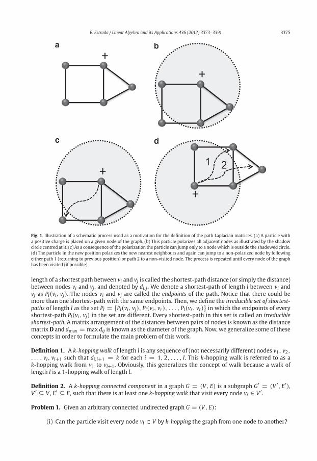
Let G = (V, E) be a simple, undirected, connected graph without self-loops and let q be a particle

that can reside in any node of the graph. Let us consider that once the particle occupies a node of the

graph it ‘polarizes’ every node separated at no more than d edges from it. For the sake of simplicity

let us consider now the case d = 1. That is, if the particle is considered to have a positive ‘charge’,

once it occupies a node vi of G, every node adjacent to vi is polarized to have positive charge (see

Fig. 1 for a pictorial representation). As a consequence of the similar polarity of all the nodes adjacent

to the particle, q can only hop to a node which is at more than one edge from its actual position. We

consider a principle of minimum distance, such as the particle will hop to any of the nearest non-

positive nodes available. Once in the new position the polarities of the nodes change correspondingly

(see Fig. 1). So, now the particle can return back to its original position or hops to any other of the

available nearest non-positive nodes. The process can be repeated from this position and so forth.

The fundamental questions that naturally arise here are the following. Can the particle be delocalized

among all the nodes of the graph? How many regions exist in a given graph such as the particle can

visit every node in a given region but not jumping from one region to another?

To warm up let us start by recalling some graph-theoretic definitions. A walk of length l is any

sequence of (not necessarily different) nodes v1, v2, . . . , vl, vl+1 such that for each i = 1, 2, . . . , lthere is a link from vi to vi+1[35]. This walk is referred to as a walk from v1 to vl+1. A path of length l

between v1 and vl+1 is a walk of length l in which all the nodes (and all the edges) are distinct. Among

all the paths between v1 and vl+1 the ones having the minimum length are called shortest-paths. The

E. Estrada / Linear Algebra and its Applications 436 (2012) 3373–3391 3375

Fig. 1. Illustration of a schematic process used as a motivation for the definition of the path Laplacian matrices. (a) A particle with

a positive charge is placed on a given node of the graph. (b) This particle polarizes all adjacent nodes as illustrated by the shadow

circle centred at it. (c) As a consequence of the polarization the particle can jump only to a nodewhich is outside the shadowed circle.

(d) The particle in the new position polarizes the new nearest neighbours and again can jump to a non-polarized node by following

either path 1 (returning to previous position) or path 2 to a non-visited node. The process is repeated until every node of the graph

has been visited (if possible).

length of a shortest path between vi and vj is called the shortest-path distance (or simply the distance)

between nodes vi and vj , and denoted by di,j . We denote a shortest-path of length l between vi and

vj as Pl(vi, vj). The nodes vi and vj are called the endpoints of the path. Notice that there could be

more than one shortest-path with the same endpoints. Then, we define the irreducible set of shortest-

paths of length l as the set Pl = {Pl(vi, vj), Pl(vi, vr), . . . , Pl(vs, vt)

}in which the endpoints of every

shortest-path Pl(vi, vj) in the set are different. Every shortest-path in this set is called an irreducible

shortest-path. A matrix arrangement of the distances between pairs of nodes is known as the distance

matrixD and dmax = max dij is known as the diameter of the graph. Now, we generalize some of these

concepts in order to formulate the main problem of this work.

Definition 1. A k-hopping walk of length l is any sequence of (not necessarily different) nodes v1, v2,. . . , vl, vl+1 such that di,i+1 = k for each i = 1, 2, . . . , l. This k-hopping walk is referred to as a

k-hopping walk from v1 to vl+1. Obviously, this generalizes the concept of walk because a walk of

length l is a 1-hopping walk of length l.

Definition 2. A k-hopping connected component in a graph G = (V, E) is a subgraph G′ = (V ′, E′),V ′ ⊆ V , E′ ⊆ E, such that there is at least one k-hopping walk that visit every node vi ∈ V ′.

Problem 1. Given an arbitrary connected undirected graph G = (V, E):

(i) Can the particle visit every node vi ∈ V by k-hopping the graph from one node to another?


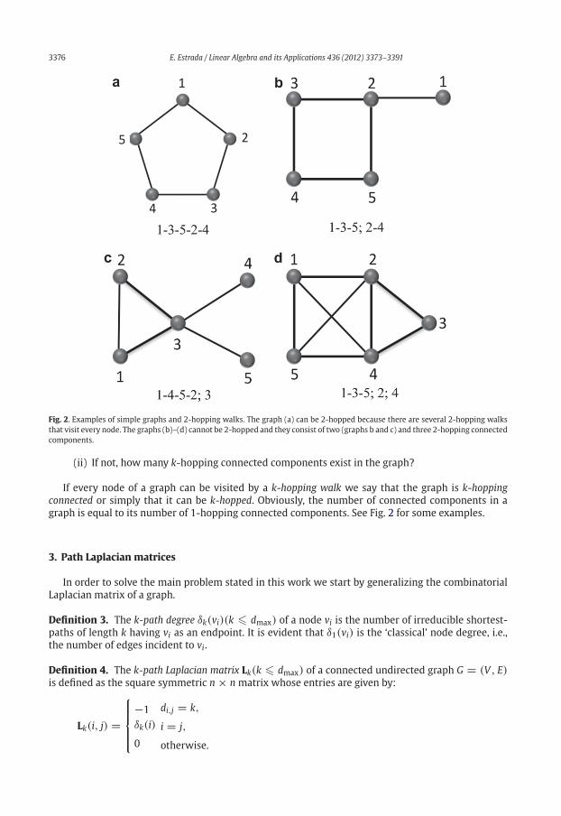
Fig. 2. Examples of simple graphs and 2-hopping walks. The graph (a) can be 2-hopped because there are several 2-hopping walks

that visit every node. The graphs (b)–(d) cannot be 2-hopped and they consist of two (graphs b and c) and three 2-hopping connected

components.

(ii) If not, how many k-hopping connected components exist in the graph?

If every node of a graph can be visited by a k-hopping walk we say that the graph is k-hopping

connected or simply that it can be k-hopped. Obviously, the number of connected components in a

graph is equal to its number of 1-hopping connected components. See Fig. 2 for some examples.

3. Path Laplacian matrices

In order to solve the main problem stated in this work we start by generalizing the combinatorial

Laplacian matrix of a graph.

Definition 3. The k-path degree δk(vi)(k � dmax) of a node vi is the number of irreducible shortest-

paths of length k having vi as an endpoint. It is evident that δ1(vi) is the ‘classical’ node degree, i.e.,

the number of edges incident to vi.

Definition 4. The k-path Laplacian matrix Lk(k � dmax) of a connected undirected graph G = (V, E)is defined as the square symmetric n × n matrix whose entries are given by:

Lk(i, j) =

⎧⎪⎪⎪⎨⎪⎪⎪⎩

−1

δk(i)

0

di,j = k,

i = j,

otherwise.


It is evident that L1 = L is the so-called combinatorial Laplacianmatrix of a graph, i.e., L1 = L = K−A.The following are the path Laplacian matrices of the graph illustrated in Fig. 2b.

L1(G)=

⎛⎜⎜⎜⎜⎜⎜⎜⎜⎜⎜⎝

1 −1 0 0 0

−1 3 −1 0 −1

0 −1 2 −1 0

0 0 −1 2 −1

0 −1 0 −1 2

⎞⎟⎟⎟⎟⎟⎟⎟⎟⎟⎟⎠

L2(G)=

⎛⎜⎜⎜⎜⎜⎜⎜⎜⎜⎜⎝

2 0 −1 0 −1

0 1 0 −1 0

−1 0 2 0 −1

0 −1 0 1 0

−1 0 −1 0 2

⎞⎟⎟⎟⎟⎟⎟⎟⎟⎟⎟⎠

L3(G)=

⎛⎜⎜⎜⎜⎜⎜⎜⎜⎜⎜⎝

1 0 0 −1 0

0 0 0 0 0

0 0 0 0 0

−1 0 0 1 0

0 0 0 0 0

⎞⎟⎟⎟⎟⎟⎟⎟⎟⎟⎟⎠

.

Definition 5. The k-path incidence matrix (k � dmax), denoted by ∇k , of a connected graph of n

nodes and p irreducible shortest-paths of length k, is a matrix of p rows and n columns in which the

rows correspond to the elements of the irreducible set of shortest-paths in the graph in which the

paths are arbitrarily oriented from head to tail and the columns correspond to the nodes of the graph,

v1, v2, . . . , vn. Then, the (i, j) entry of ∇k is defined as:

∇k(i, j) =

⎧⎪⎪⎪⎨⎪⎪⎪⎩

1

−1

0

if vj is the head of the irreducible shortest path pi,

if vj is the tail of the irreducible shortest path pi,

otherwise.

Definition 6. The k-path matrix (k � dmax), denoted by Pk , of a connected graph of n nodes is the

square, symmetric, n × nmatrix whose entries are defined as follows:

Pk(i, j) =⎧⎨⎩

1

0

if dij = k,

otherwise.

Notice that δk(vi) = (1TPk)i, where 1 is an all-ones column vector. Also notice that:

D =dmax∑k=1

kPk. (1)

It can be easily verified that

Lk = ∇Tk ∇k = �k − Pk, (2)

where �k = diag(1TPk

). It can be seen that

yTLky = 1

2

∑i,j∈Pk(vi,vj)

(yi − yj)2 (3)

for any column vector y. As a consequence, the k-path Laplacian matrices Lk are positive semidefinite.

As for the case of the combinatorial Laplacian, the path Laplacian matrices are singular M-matrices.

Let:

SpLk =⎛⎝ λ1(Lk) λ2(Lk) · · · λn(Lk)

m [λ1(Lk)] m [λ2(Lk)] · · · m [λn(Lk)]

⎞⎠ (4)

be the k-path Laplacian spectrum of a graph G, where λj(Lk) is the jth eigenvalue of the matrix Lk and

m[λj(Lk)] is its multiplicity. Let us order the eigenvalues of the k-Laplacian matrix in a nondecreasing


manner as: λ1(Lk) � λ2(Lk) � · · · � λn(Lk). Because the Lk matrices are positive semidefinite their

eigenvalues are nonnegative. It is easy to see that Lk1T = 0, which means that 0 is an eigenvalue of Lk

with a 1 eigenvector.

4. When can a graph be k-hopped?

The solution of the problem of k-hopping a graph is given in the following theorem which is the

main result of this work.

Theorem1. The number of k-hopping connected components in a connected undirected graph G = (V, E)is given by ηk(G) = m [λ1(Lk) = 0].

Proof. Let {y1, y2, . . . yn} be an orthogonal basis of Rn such that Lkyj = λj(Lk)yj . Now by using the

Rayleigh–Ritz Principle we obtain

λ1(Lk) = miny∈Rn\{0}

yTLky

yTy= min

y∈Rn\{0}

∑p,q∈Pk(vp,vq) (yp − yq)

2

∑p∈V y2p

. (5)

Let y be an eigenvector of Lk with eigenvalue λ1(Lk) = 0. This means that

yTLky = ∑p,q∈Pk(vp,vq)

(yp − yq)2 = 0, (6)

which happens if and only if, yp = yq for each pair of nodes which are connected by a shortest-path of

length k. Now, let us assume that the graph is k-hopping connected. Then, because every pair of nodes

is connected by paths of length ck, we have that yp = yq �= 0 for every pair of nodes in the graph.

Consequently, y is a constant vector spanning a one-dimensional eigenspace.

Now let j > 1 and let us assume that the graph has g k-hopping connected components

L1k , L2k , . . . , L

gk . Then, the k-Laplacian matrix can be written as:

Lk =

⎛⎜⎜⎜⎜⎜⎜⎜⎝

L1k 0 · · · 0

0 L2k · · · 0

......

. . ....

0 0 · · · Lgk

⎞⎟⎟⎟⎟⎟⎟⎟⎠

.

Following similar arguments as for the case of the k-hopping connected graph it can be seen that Lkhas g orthogonal eigenvectors yj of eigenvalue 0, such that yp = yq �= 0 for each pair of nodes which

are in the same k-connected component of the graph and zero otherwise. �

Let us return to the example of the graph illustrated in Fig. 2. In Table 1 we give the eigenvalues of

these four graphs where it can be seen that the graph 2(a) has only one 2-hopping connected com-

ponent, i.e., it is a 2-hopped graph; graphs 2(b) and 2(c) have two 2-hopping connected components

and graph 2(d) has three 2-hopping components. The zeroes of the 2-path Laplacin matrices of these

graphs are boldfaced in Table 1.

Table 1

Eigenvalues of the 2-path Laplacian matrix for the graph illustrated in Fig. 2.

2(a) 2(b) 2(c) 2(d)

0.000 0.000 0.000 0.000

1.382 0.000 0.000 0.000

1.382 2.000 2.000 0.000

3.618 3.000 4.000 1.000

3.618 3.000 4.000 3.000


5. Path Laplacians and consensus in multi-agent systems

In Section 1 we mention the consensus problem as one of the many processes which are usually

modeled by means of the Laplacian matrix of a graph. In a multi-agent system, “consensus” means an

agreement regarding a certain quantity of interest that depends on the state of individual agents. In

this problem the agents are represented by the nodes of the network and the links represent some kind

of interaction among them. This is usually the case of a series of autonomous vehicles which perform

activities through cooperative teamwork in civilian andmilitary applications. This coordinated activity

allows them to performmissions with greater efficacy and operational capability than if they perform

solo missions. This kind of consensus models has applications in a variety of areas such as collective

behavior of social networks, flocks and swarms, sensor fusion, synchronization of coupled oscilla-

tors, formation control of multirobot systems, spatial rendezvous, cooperative control, among others

[10–17].

If we consider a set of n agents forming a network, the collective dynamics of the group of agents

is represented by the following equations for the continuous-time case:

ϕ = −Lϕ, ϕ(0) = ϕ0, (7)

where ϕ0 is the original distribution. In general, we will consider that the agents start with a random

configuration which here will be the random labels of the nodes. Consensus is reached if, for all ϕi(0)and all i, j = 1, . . . , n,

∣∣ϕi(t) − ϕj(t)∣∣ → 0 as t → 0. The discrete-time version of the model has the

form

ϕi(t + 1) = ϕi(t) + ε∑j∼i

Aij

[ϕj(t) − ϕi(t)

], ϕ(0) = ϕ0 (8)

whereϕi(t) is the value of a quantitative measure on node i, ε > 0 is the step-size, and j ∼ i indicates

that node j is connected to node i. It has been proved that the consensus is asymptotically reached

in a connected graph for all initial states if 0 < ε < 1/δmax, where δmax is the maximum degree of

the graph [10]. The discrete-time collective dynamics of the network can be written in matrix form as

[10]:

ϕ(t + 1) = Pϕ(t), ϕ(0) = ϕ0, (9)

where P = I − εL, and I is the n × n identity matrix. The matrix P is referred to as the Perron matrix

of the network with parameter 0 < ε < 1/δmax. For any connected undirected graph the matrix P

is an irreducible, doubly stochastic matrix with all eigenvalues μj in the interval [−1, 1] and a trivial

eigenvalue of 1. The relation between the Laplacian and Perron eigenvalues is given by: μj = 1− ελj .

5.1. Consensus with long-range interactions

In the ‘classical’ problem of consensus in a networkedmulti-agent system it is considered that only

pairs of agents directly connected to each other interact in the search of agreement. However, in many

real-world situations the agents are exposed not only to their closest contacts but also to long-range

interactions with other agents in the system. For instance, let us consider a multi-agent networked

systems inwhich the agent i emits a signalwith a propagation radius r1. Such a signal can be of any kind

ranging from electromagnetic signals to the visual radius of an individual. Every other node j which

is at a distance rij � r1 is considered to be connected to node i and consequently they are mutually

influenced, such that they can reach an agreement as described by Eq. (8). This process is illustrated in

Fig. 3a. Now let us suppose that the agent i also emits a weaker signal with a radius r2 > r1. This is, for

instance, the case in most of real-world situations where not only one signal is emitted but a packet of

waves whose intensity decreases with the distance from the source. Let us consider a node k which is

at distance r1 < rik � r2 from i. Obviously, k is not connected to i because rik > r1, but it still makes

a ‘long-range’ influence on node i, which can be considered as a weakest type of connection among

them (see Fig. 3b).


Fig. 3. Schematic illustration of the linking between agents that gives rise to the consensus in networked multi-agent systems.

(a) Every node emits a signal of radius r1 which is reached by any other node at distance shorter than r1 from the emitter. Two nodes

i and j are connected if and only if rij � r1. (b) The node i emits now two signals with radii r1 and r2, which generate two different

kinds of connectivity. As before, nodes i and j are connected because rij � r1. Now, nodes i and k are ‘weakly’ connected because

r1 < rik � r2. The two types of connection can be considered as weighted links in which w(i, j) = 1 and 0 < w(i, k) < 1, with w

standing for the weight of the link.

We assume that the long-range interactions are weaker than the short-range ones. Now we can

assume that the agents in the system reach consensus under the influence of close and long-range

contacts. This generalized consensus model can be described by:

ϕ(t + 1) = PGϕ(t), ϕ(0) = ϕ0, (10)

where

PG = I − ε�∑

k=1

ckLk, (11)

where 1 � � � dmax. Obviously, if � = 1 we recover the equation for the consensus in a network

without long-range interactions. Finally, in order to guarantee that thematrix PG is stochastic we have

to select the parameter ε such as

0 < ε <

⎡⎣

�∑k=1

δmax(k)

⎤⎦

−1

. (12)

5.2. On long-range coefficients

An important aspect of the current theory in which agents are influenced not only by nearest

neighborsbut also through long-range interactions is thedeterminationof the coefficients ck appearing

in (11). These coefficients are expected to give more weight to the shorter than to the longer range

interactions. That is, the influence of an agent over another decays with the separation among them.

Herewepropose twodifferent approaches, identifying themwithphysical and socialways of influence,

respectively.

5.2.1. Physical influence

In many physical scenarios the communication among the agents in the system displays spatial

decay. This situation is observed in many man-made and naturally evolved systems. In many of them

some kind of consensus among the agents of the system can take place, such as in the following

examples mentioned here for the sake of illustration:

(1) Sensor systems [36]. Sensors far away from a target display low signal-to-noise ratio due to

the spatial decay of the signal energy.

(2) Earthquakes [37]. Aftershocks follow a well-defined spatial decay of the form r−α , where r is

the distance from the main shock.


(3) Neural connectivity [38]. The interconnectivity between certain neurons in mammalian neo-

cortex decays exponentially with the intersomatic distance.

(4) Population spatial synchrony [39]. The correlated fluctuations in abundance or some other

population property exhibited by many species, including insects, fish, birds, mammals and

human pathogens, decays with the distance among populations.

Thus, we can consider that for two agents separated at distance k their interaction decays either

as a power-law of the form: ck = k−α , or as an exponential of the form ck = e−αk, where α > 0

is a parameter that depends on the specific situation to be modeled. If we are now interested in the

analysis of the consensus of the agents in this networked system we have to analyze the following

forms of (11):

PG = I − ε�∑

k=1

e−αkLk, (13)

PG = I − ε�∑

k=1

k−αLk. (14)

5.2.2. Social influence

Individuals in a social network can be influenced by some kinds of interactions which differ signif-

icantly from that previously analyzed for physical systems. In such social networks nodes represent

individuals which are connected by some social tie, e.g., friendship, family relation, collaboration, etc.

Obviously, individuals which are directly connected in their social network usually influence each

other. However, the way in which two individuals not directly connected in the social network in-

fluence each other is not evident. We have previously assumed [40] on the basis of vast empirical

evidence that this ‘long-range’ influence among individuals can be though as a preconditioner of new

social relations. That is, if two individuals influence each other they have larger chances of becoming

friends or collaborators than two otherswhich have nullmutual influence. There are enough empirical

evidences to support the idea that new social ties are created as an ‘investment’ for the future, not only

among humans but also among some other primates (see [40] and references therein). Then, we have

considered such a process as the analogy in which the time value of money, in particular the future

value of a growing annuity, is determined in quantitative finance. However, instead of money we have

generalized the process by assuming that an individual lends a piece of information to another. This

information has a future value FVI which is determined, according to the quantitative finance theory,

by its present value PVI, the interest rate r and the number of time periods t at which the information

is lent. That is [40],

FVI = PVI · (1 + r)t . (15)

If the node i lends some information to node j, it is assumed that the information flows through the

shortest path connecting both nodes [40]. The information is passed using a discrete time in which

every step in the path is considered to have a unit time. Then, in a process of lending information from

node v1 to node vl+1, the information is first transferred to node v2 with a value A and an interest rate

r. The present value of the information in the hands of node v2 is A/(1 + r). Then node v2 enriched

this information by a given value g, which we will designate as the growing rate of the information

[40]. When the node v2 lends this information to node v3 with the same interest and growing rates,

the informationwill have a value A(1 + g)/(1 + r)2 in the hands of node v3. As every node in the path

lends the information to its nearest neighbor with the interest r and growing rate g, the information in

the hands of the borrower node vl+1 will have a value of A(1 + g)l−1/(1 + r)l . The cumulative present

value of the information in this process is given by the sum of all the values at the nodes of the chain

[40]:

PVI = A/(1 + r) + A(1 + g)/(1 + r)2 + · · · + A(1 + g)l−1/(1 + r)l. (16)


If the growing and interest rates are the same, i.e., g = r, the present value of the information is

simplified to:

PVI = A · l/(1 + r). (17)

Then, the future value of the information is given as [40]:

FVI = A · l · (1 + r)l−1. (18)

We consider that A ≡ 1 for the sake of simplicity. Then, because in a connected network any two

nodes i and j are separated by a shortest-path distance dij , the expression for the future value of the

information transmitted from i to j is given by:

FVI(i, j) = dijxdij−1, (19)

where x = 1 + r = 1 + g.

Consequently, we can consider that themutual influence between two nodes separated at distance

k is given by the future value of the investment that the creation of a new link will represent to them.

Mathematically, thismeans that we define the coefficients in (11) as: ck�2 = kxk−1 and c1 = 1, where

0 � x < 1/2 is an empirical parameter accounting for the strength of interaction between two nodes

at distance k. Thus, if are interested in analyzing the consensus among the agents in a social network

we have to analyse the following form of (11):

PG = I − ε

⎛⎝L +

�∑k=2

kxk−1Lk

⎞⎠ . (20)

5.3. Simulations

In order to illustrate the effects of long-range interactions on the consensus among agents in a

complex network we study two types of random networks: the Erdös–Rényi (ER) graphs [41] and

the Barabási–Albert (BA) [42] ones with 1000 nodes and average degree equal to 8. In the ER graphs

a group of nodes are connected randomly forming a graph with Poisson degree distribution. In the

case of BA model, nodes are connected following a preferential attachment algorithm such that the

resulting graph displays a power-law degree distribution of the type p(δ) ∼ δ−3, where p(δ) is the

probability of finding a node of degree δ in the graph. For the problem of consensus we analyze the

time evolution of the vector ϕ taken at the beginning as the random labeling of the nodes. Consensus

is considered to be reached if∣∣ϕi(t) − ϕj(t)

∣∣ � 10−5 for every pair of nodes in the graph. The time at

which this consensus is reached is reported as the consensus time.

In Fig. 4 we illustrate the results of the simulations for the ER and BA graphs without the consider-

ation of long-range influences, e.g., Eq. (11) with � = 1. The consensus in the network with Poisson

degree distribution is reached only after 15,000 time steps. In contrast, the consensus is obtained for

the network with power-law degree distribution at about 8000 time steps. This difference is basically

due to the existence of highly connected nodes in the BA network. These hubs influence many nodes

at the same time, which allow them to reach consensus in a faster way than in a more ‘homogeneous’

network like ER ones.

5.3.1. Physical influence

We turn now our attention to the study of consensus under the influence of both close and long-

range interactions. We start by assuming that there is a spatial decay of the influence among agents

which follows either an exponential or a power-law. That is, we consider that one target-agent in

the network is influenced by all its nearest neighbors. In addition, it is also influenced by all the

other agents in the system. This influence decays with the distance at which the agents are separated

by following either an exponential or power-law decays. For the analysis of consensus we use the

generalized Perron matrices (13) and (14) in which � = dmax. A value of ε = 4 × 10−4 is used in all

the simulations. We remark that the ER and BA networks used here for illustration have dmax = 7 and


Fig. 4. State evolution corresponding to an ER (left) and BA (right) randomnetworkswith 1000 nodes and 4000 links. The simulations

were performed using Eq. (9).

dmax = 5, respectively. The values of [∑�k=1 δmax(k)]−1 for these two networks are 4.755× 10−4 and

4.198 × 10−4, respectively, which are larger than the value of ε used for the simulations. In Fig. 5 we

illustrate the results of these simulations for the exponential (left) and power-law (right) decays and

the values of α = 2.0 (top) and α = 1.5 (bottom). When there is an exponential spatial decay of the

signal the time at which consensus is reached drops frommore than 15,000 to about 5000 time steps

for α = 1.5. Themost dramatic reduction in the consensus time is observed for the power-law spatial

decay. Here the time necessary for reaching consensus is reduced 75 times respect to the case where

no long-range influences are allowed. That is, consider a systemhaving a Poisson degree distribution in

which the consensus among the agents directly connected is reached at a time t. If the system displays

spatial power-law decay of the physical signal among the agents, the consensus is reached in a time

t/75. For instance, in a system of autonomous vehicles performing a coordinated mission this will

represent a tremendous saving of time and increase of the efficiency of that system.

The analysis of the long-range physical influence in BA networks shows similar dramatic reduc-

tions in the time for consensus in relation to the case in which only close contacts are considered. In

Fig. 6 we illustrate these results, where it can be seen that the use of power-law spatial decay with

α = 1.5 drops the consensus time to about t/53 respect to the case where only close contacts are

considered.

5.3.2. Social influence

When studying the consensus in a network under the influence of long-range social interactions

we have to deal with the parameter x which controls the feasibility of these interactions. That is, for

x = 0 there is no long-range influence among the agents and the model (9) is recovered. As the value

of x increases we give more chances to pairs of agents at long distances to influence each other. Thus

we study here the same two networks previously analyzed by considering the values of x = 0.1,x = 0.25 and x = 0.5. As before a value of ε = 4 × 10−4 is used in all the simulations. As can be

seen in Fig. 7 even for small values of x there is a dramatic reduction in the consensus time for both

types of networks. For x = 0.5 these reductions are of the order of t/375 respect to the times obtained

when no long-range influences are considered. These reductions are far more dramatic than those

observed for the cases of physical influence among the agents. Then, if you wonder about the causes

why consensus in social networks is sometimes reached in so effective way, e.g., in recent uprising

in several Arab countries or anticapitalist protests in developed countries, you must think about the

effects of long-range influences.


Fig. 5. State evolution of an ERnetworkwith 1000 nodes, 4000 links and diameter 7 by considering both close and long-range physical

influences. The simulations were performed by using Eq. (10) and the generalized Perron matrices (13) (left) and (14) (right) using

α = 2.0 (top) and α = 1.5 (bottom). In all cases the value ε = 4 × 10−4 was used (see text).

Another area in which long-range influence of nodes can be important for reaching consensus is

the case of networks having highly connected clusters which are poorly linked among them. These

highly connected clusters are usually known in network theory as communities, and they represent a

variety of entities such as social groups, genes with similar functions or groups of corporations of the

same economic sector [43–46]. Because the nodes in one particular community are well-connected to

each other it is relatively easy to reach consensus among them. However, consensus between nodes

in different communities is a more difficult task if only nearest-neighbors influence is allowed. Taking

into account that most of social networks are highly clustered into different social communities, how

is it possible to reach social consensus in relatively short times? An intuitive answer to this question

is that individuals are not only influenced by the members of their communities but by individuals

not far from them in other social groups. For instance, in Fig. 8 we illustrate the results obtained for

a network formed by two identical chunks connected by only one link. Both parts of the network are

created as ER random graphswith 100 nodes and 400 links. The network has a diameter equal to 7 and

we use a value of ε = 0.028 in all simulations, which is smaller than [∑�k=1 δmax(k)]−1. As can be seen

when only nearest neighbors are considered the consensus is obtained after more than 100,000 time


Fig. 6. State evolution of a BA networkwith 1000 nodes, 4000 links and diameter 5 by considering both close and long-range physical

influences. The simulations were performed by using Eq. (10) and the generalized Perron matrices (13) (left) and (14) (right) using

α = 2.0 (top) and α = 1.5 (bottom). In all cases the value ε = 4 × 10−4 was used (see text).

steps. That is, there is practically no absolute consensus among the individuals in the two separated

clusters. However, this time is reduced very dramaticallywhen long-range influence among the agents

enters into play. For a value of x = 0.1 the consensus is reached at about 7000 time steps and this

time is reduced to only 60 time steps for x = 0.5. This represents an improvement of more than 1666

times in the consensus time.

In Fig. 9 we illustrate the results for a real-world social network, which is well known for having at

least two well defined communities. It corresponds to a friendship network in a karate club in US and

it is known as the Zachary karate club network [47]. This network is characterized by the existence of

a group of followers of the instructor and another group of followers of the administrator of the club.

The polarization between the two groups was clear after the instructor and the administrator had a

conflict which divided the club into two well defined communities characterized by the respective

followers of each ‘leader’. The network has 34 nodes and 78 links, a diameter equal to 5 and we have

used ε = 0.012 in all simulations, which is smaller than [∑�k=1 δmax(k)]−1. As can be seen in Fig. 9

the consensus in the network after considering the long-range influence of the agents is obtained 56

times faster than if only nearest neighbors are considered for a value of x = 0.5.


Fig. 7. State evolution of ER (left) and BA (right) networks with 1000 nodes, 4000 links and diameters 7 and 5, respectively, by

considering both close and long-range social influences. The simulations were performed by using Eq. (10) and the generalized

Perron matrix (20) by using x = 0.1 (top), x = 0.25 (center), and x = 0.5 (bottom).


Fig. 8. State evolution of the consensus among agents in a network formed by two identical blocks of 100 nodes and 400 links each

(displayed at the top). Each block is created by an ER process and they are linked together by mean of only one link. The simulations

are performed by using Eq. (10) and the Perron matrix (20) for different values of x. The diameter of this network is 7 and we use

ε = 0.028 in all simulations.


Fig. 9. State evolution of the consensus among agents in a real-world social network formed by 34 individuals and its 78 friendship

links in a karate club in US. The simulations are performed by using Eq. (10) and the Perron matrix (20) for different values of x. The

diameter of this network is 5 and we use ε = 0.012 in all simulations.

6. On computation of the path Laplacian matrices

In order to compute the kth path Laplacian matrix of a graph we need to identify all pairs of nodes

at distance k. In the most complete scenario we will be interested in obtaining all path Laplacian ma-

trices for 1 � k � dmax. In this case it is better to obtain the distance matrix D of the graph and

obtaining each k-path matrix by using Definition 6. In order to obtain the distance matrix we have

to solve the all-pairs shortest paths (APSP) problem, for which there are many algorithms available

in the literature [48]. The APSP problem appears in many other areas of complex networks analy-

sis, such as in the study of distance-based centrality measures, average path length and small-world

phenomenon, among others. The most used of these algorithms was devised in 1959 by Dijkstra and

it computes APSP in O(mn + n2 log n), where m is the number of links [49]. There are many im-

provements of this algorithm as well as many others that beat this worst case running time of the


Dijkstra algorithm. For instance, for sparse networks having m = o(n log n) Pettie has designed an

algorithm that finds APSP in O(mn + n2 log log n) for directed arbitrarily weighted graphs [50]. In the

case of undirected graphs with integer weights Thorup has proposed algorithms with running times

of O(mn) [51,52]. An important result for unweighted graphs as the ones studied in this work is the

one proving that if matrix multiplication can be performed in O(M(n)), then the APSP problem for

unweighted directed graphs can be solved in O(√n3M(n)) and for unweighted undirected ones in

O(M(n)), where we have ignored the polylogarithm function appearing in the expressions [53–57].

One of the current best upper bounds on general matrix multiplication is M(n) = O(n2.376) obtainedby Coppersmith and Winograd [58], while for a sparse networks Yuster and Zwick [59] have found

an estimate of M(n) = O(m0.7n1.2 + n2+o(1)), which for m � n1.14 makes the multiplication in an

almost optimal number of operations: M(n) = O(n2+o(1)), and for m � n1.68 it still performs in

a better way than the method of Coppersmith and Winograd [58]. However, as we have indicated

previously we not necessarily would be interested in computing all path-Laplacian matrices but only

a few of them. For instance, if there is evidence that a particular signal does not propagates beyond

the second nearest neighbors we would only need to compute L and L2, which will alleviate the

calculations.

This situation is not different to what is found in many other calculations performed for the study

of complex networks [60]. For instance for computing closeness centrality we need to compute all

distances from a given node, for the average path length we need to compute the distances among

all pairs of nodes, and for the calculation of the betweenness centrality we need to calculate all the

shortest paths passing through a given node. In the last case, for instance, the most efficient algorithm

designed so far obtains the betweenness centrality of every node in O(mn + n2 log n) for weighted,

and in O(mn) for unweighted graphs [61]. All these methods, including the use of path Laplacians,

will benefit from the development of new methods for solving the APSP problem (see [62] and the

references therein).

7. Conclusions and future outlook

We have introduced here the concept of path-Laplacian matrices, which naturally generalizes the

combinatorial Laplacian widely used in mathematics, physics, computer sciences and engineering.

The new concept has been motivated by studying the k-hopping of a graph, which consists in know-

ing whether every node of a graph can be visited by jumping from one node to another at distance

k from it. It is impossible at this stage to foresee every single application of this concept in differ-

ent scenarios. We have provided here an example in which the path-Laplacian matrices are impor-

tant for understanding how the consensus is reached in some real-world scenarios where not only

nearest neighbors but also long-range interactions of different kinds can be present. The hypoth-

esis stating that consensus is reached by the influence of both nearest- and nonnearest neighbors

can be tested experimentally in physical and social scenarios, making it ‘falsifiable’ as required for

any scientific theory. Another area in which path-Laplacian matrices can find a niche for applica-

tions is in the study of synchronization in complex networks. It is hard to believe that the synchro-

nization observed among crickets, fireflies, birds and fishes is reached by the influence of nearest

neighbors only. Thus, the consideration of the influence of nonnearest neighbors through the use of

path-Laplacian matrices in synchronization models can help to understand such complex dynami-

cal processes. On the more practical side we predict the possibility of designing algorithms in which

the long-range interactions among agents is exploited. As an example we can consider a group of

robots for which consensus need to be obtained. By considering not only robots which are directly

connected to each other according to a given signal, but also those which are in the second or third

neighborhood (as in Fig. 3), a faster consensus can be reached for a given activity. In closing, we believe

that the path-Laplacian matrices will be an important addition to the large arsenal of graph-theoretic

and algebraic tools currently used in many scientific disciplines. Last but not least, the study of the

mathematical properties of these matrices is a completely new avenue in the field of algebraic graph

theory.


Acknowledgement

Wewould like to thankMichele Benzi (Emory) for carefully reviewing the paper and offering useful

suggestions that contributed to a better presentation of this work. Gil Strang (MIT) is also thanked for

revising an early draft of this work.We also thank partial financial support fromNew Professor’s Fund,

University of Strathclyde and from the project Mathematics of Large Technological Evolving Networks

(MOLTEN) supported by the Engineering and Physical Sciences Research Council and the Research

Councils UK Digital Economy programme, with Grant Ref. EP/I016058/1.

References

[1] B. Mohar, The Laplacian spectrum of graphs, in: Y. Alavi, G. Chartrand, O. Ollermann, A. Schwenk (Eds.), Graph Theory, Combi-natorics, and Applications, Wiley, New York, 1991, pp. 871–898.

[2] R. Merris, Laplacian matrices of a graph: a survey, Linear Algebra Appl. 197 (1994) 143–176.[3] C. Godsil, G. Royle, Algebraic Graph Theory, Springer-Verlag, Berlin, 2001.

[4] F.R.K. Chung, Spectral Graph Theory, American Mathematical Society, 1996.

[5] M. Fiedler, Algebraic connectivity of graphs, Czechoslovak Math. J. 23 (1973) 298–305.[6] M.C.V. Nascimento, A.C.P.L.F. de Carvalho, Spectral methods for graph clustering. A survey, Eur. J. Oper. Res. 211 (2011) 221–231.

[7] M. Belkin, P. Niyogi, Laplacian eigenmaps for dimensionality reduction data representation, Neural Comput. 15 (2003) 1373–1396.

[8] Y. Ghanbari, P. Papamichalis, L. Spence, Graph-Laplacian features for neural waveform classification, IEEE Trans. Biomed. Eng.58 (2011) 1365–1372.

[9] P. Niyogi, S. Smale, S. Weinberger, A topological view of unsupervised learning from noisy data, SIAM J. Comput. 40 (2011)646–663.

[10] R. Olfati-Saber, J. Alex Fax, R.M. Murray, Consensus and cooperation in networked multi-agent systems, Proc. IEEE 95 (2007)

215–233.[11] R. Olfati-Saber, Flocking for multi-agent dynamic systems: algorithms and theory, IEEE Trans. Automat. Control 51 (2006)

401–420.[12] Y. Hatano, M. Mesbahi, Agreement over random networks, IEEE Trans. Automat. Control 50 (2005) 1867–1872.

[13] M. Mesbahi, M. Egerstedt, Graph Theoretic Methods in Multiagent Networks, Princeton University Press, 2010.[14] I.I. Blekhmann, Synchronization in Science and Technology, American Society of Mechanical Engineers, 1988.

[15] A. Pikovsky, M. Rosenblum, J. Kurths, Synchronization: A Universal Concept in Nonlinear Sciences, Cambridge University Press,

Cambridge, 2001.[16] S. Boccaletti, J. Kurths, G. Osipov, D.L. Valladares, S.C. Zhou, The synchronization of chaotic systems, Phys. Rep. 366 (2002) 1–101.

[17] A. Barrat, M. Barthélemy, A. Vespignani, Dynamical Processes on Complex Networks, Cambridge University Press, Cambridge,2008.

[18] M. Sipser, D.A. Spielman, Expander codes, IEEE Trans. Inform. Theory 42 (1996) 1710–1772.[19] A. Lubotzky, R. Phillips, P. Sarnak, Ramanujan graphs, Combinatorica 8 (1988) 261–277.

[20] L. Donetti, N. Franco, M.A. Muñoz, Optimal network topologies: expanders, cages, Ramanujan graphs, entangled networks and

all that, J. Stat. Mech. (2006) P08007[21] H. Shlomo, N. Linial, A. Wigderson, Expander graphs and their applications, Bull. Am. Math. Soc. 43 (2006) 439–561.

[22] U. Smilansky, Quantum chaos on discrete graphs, J. Phys. A 40 (2007) F621–F630.[23] S.L. Braunstein, S. Ghosh, S. Severini, The Laplacian of a graph as a densitymatrix: a basic combinatorial approach to separability

of mixed states, Ann. Comb. 10 (2006) 291–317.[24] P. Kurasov, Graph Laplacians and topology, Ark. Mat. 46 (2008) 95–111.

[25] K. Woong, Combinatorial Green’s function of a graph and applications to networks, Adv. Appl. Math. 46 (2011) 417–423.

[26] N. Trinajstic, D. Babic, S. Nikolic, D. Plavsic, D. Amic, Z. Mihalic, The Laplacian matrix in chemistry, J. Chem. Inf. Comput. Sci. 34(1994) 368–376.

[27] D.J. Klein, M. Randic, Resistance distance, J. Math. Chem. 12 (1993) 81–85.[28] W. Xiao, I. Gutman, Resistance distance and Laplacian spectrum, Theor. Chem. Acc. 110 (2003) 284–289.

[29] E. Estrada, N. Hatano, Topological atomic displacements, Kirchhoff andWiener indices ofmolecules, Chem. Phys. Lett. 486 (2010)166–170.

[30] F. Valerio, Improved biological network reconstruction using graph Laplacian regularization, J. Comput. Biol. 18 (2011) 987–996.

[31] E. Estrada, N. Hatano, A vibrational approach to node centrality and vulnerability in complex networks, Physica A 389 (2010)3648–3660.

[32] S. Calderara, U. Heinemann, A. Prati, R. Cucchiara, N. Tishby, Detecting anomalies in people’s trajectories using spectral graphanalysis, Comput. Vis. Im. Understand. 115 (2011) 1099–1111.

[33] K.M. Taylor, M.J. Procopio, C.J. Yong, F.G. Meyer, Estimation of arrival times from seismic waves: a manifold-based approach,Geophys. J. Int. 185 (2011) 435–452.

[34] D. Volchenkov, Randomwalks and flights over connected graphs and complex networks, Commun. Nonlinear Sci. Numer. Simul.16 (2011) 21–55.

[35] D. Cvetkovic, P. Rowlinson, S. Simic, Eigenspaces of Graphs, Cambridge University Press, Cambridge, 1997.

[36] X. Chang, R. Tan, G. Xing, Z. Yuan, C. Lu, Y. Chen, Y. Yang, Sensor placement algorithm for fusion-based surveillance networks,IEEE Trans. Parallel Distrib. Syst. 22 (2011) 1407–1414.

[37] K.R. Felzer, E.E. Brodsky, Decay of aftershock density with distance indicates triggering by dynamic stress, Nature 441 (2006)735–738.


[38] A.M. Packer, R. Yuste, Dense, unspecific connectivity of neocortical parvalbumin-positive interneurons: a canonical microcircuit

for inhibition?, J. Neurosci. 31 (2011) 13260–13271.[39] A. Liebhold,W.D. Koenig, O.N. Bjørnstad, Spatial synchrony inpopulationdynamics, Ann. Rev. Ecol. Evol. Syst. 35 (2004) 467–490.

[40] E. Estrada, F. Kalala-Mutombo, A. Valverde-Colmeiro, Epidemic spreading in networks with nonrandom with long-range inter-actions, Phys. Rev. E 84 (2011) 036110

[41] P. Erdös, A. Rényi, On random graphs, Publ. Math. 6 (1959) 290–297.

[42] A.-L. Barabási, R. Albert, Emergence of scaling in random networks, Science 286 (1999) 509–512.[43] S.E. Schaeffer, Graph clustering, Comput. Sci. Rev. 1 (2007) 27–64.

[44] N. Gulbahce, S. Lehmann, The art of community detection, Bio Essays 30 (2008) 934–938.[45] M.A. Porter, J.-P. Onnela, P.J. Mucha, Communities in networks, Notices Amer. Math. Soc. 56 (2009) 1082–1097., 1164–1166.

[46] S. Fortunato, Community detection in graphs, Phys. Rep. 486 (2010) 75–174.[47] W. Zachary, An information flow model for conflict and fission in small groups, J. Anthropol. Res. 33 (1977) 452–473.

[48] B.V. Cherkassky, A.V. Goldberg, T. Radzik, Shortest paths algorithms: theory and experimental evaluation, Math. Program. 73(1996) 129–174.

[49] E.W. Dijkstra, A note on two problems in connexion with graphs, Numer. Math. 1 (1959) 269–271.

[50] S. Pettie, A faster all-pairs shortest path algorithm for real-weighted sparse graphs, Lect. Notes Comput. Sci. 2380 (2002) 85–97.[51] M. Thorup, Undirected single-source shortest paths with positive integer weights in linear time, J. ACM 46 (1999) 362–394.

[52] M. Thorup, Floats, integers, and single source shortest path, J. Algorithms 35 (2000) 189–201.[53] Z. Galil, O. Margalit, Witnesses for Boolean matrix multiplication, J. Complexity 9 (1993) 201–221.

[54] R. Seydel, On the all-pairs-shortest-path problem in unweighted undirected graphs, J. Comput. Syst. Sci. 51 (1995) 400–403.[55] N. Alon, M. Naor, Derandomization, witnesses for Boolean matrix multiplication and construction of perfect has functions,

Algorithmica 16 (1996) 434–449.

[56] N. Alon, Z. Galil, O. Margalit, On the exponent of the all pairs shortest path problem, J. Comput. Syst. Sci. 54 (1997) 255–262.[57] Z. Galil, O. Margalit, All pairs shortest paths for graphs with small integer length edge, J. Comput. Syst. Sci. 54 (1997) 243–254.

[58] D. Coppersmith, S. Winograd, Matrix multiplication via arithmetic progression, J. Symbolic Comput. 9 (1990) 251–280.[59] R. Yuster, D. Zwick, Fast sparse matrix multiplication, ACM Trans. Algorithms 1 (2005) 2–13.

[60] R. Jacob, D. Koschützki, K.A. Lehman, L. Peeters, D. Tenfelde-Podehl, Algorithms for centrality indices, in: U. Brandes, T. Erlebach(Eds.), Network Analysis. Methodological Foundations, Springer-Verlag, Berlin, 2005, pp. 62–82.

[61] U. Brandes, A faster algorithm for betweenness centrality, J. Math. Sociol. 25 (2001) 163–177.

[62] A. Gubichev, S. Bedathur, S. Seufert, G.Weikum, Fast and accurate estimation of shortest paths in large graphs, in: CIKM’10, Proc.19th ACM Int. Conf. Inf. Know. Manag., Toronto, Ontario, Canada, October 26–30, 2010, pp. 499–508.

Documents

Linear Algebra and its Applications - Estrada Lab · Linear Algebra and its Applications 436 (2012) 3373–3391 Contents lists available at SciVerse ScienceDirect Linear Algebra and