Embed Size (px)
Citation preview

Linear Algebra

This page intentionally left blank
Linear Algebra
An Introduction
Second Edition
RICHARD BRONSONProfessor of Mathematics
School of Computer Sciences and Engineering
Fairleigh Dickinson University
Teaneck, New Jersey
GABRIEL B. COSTAAssociate Professor of Mathematical Sciences
United States Military Academy
West Point, New York
Associate Professor of Mathematics and Computer Science
Seton Hall University
South Orange, New Jersey
AMSTERDAM • BOSTON • HEIDELBERG • LONDONNEW YORK • OXFORD • PARIS • SAN DIEGO
SAN FRANCISCO • SINGAPORE • SYDNEY • TOKYOAcademic Press is an imprint of Elsevier

Acquisitions Editor Tom SingerProject Manager A.B. McGeeMarketing Manager Leah AckersonCover Design Eric DeCiccoComposition SPi Publication ServicesCover Printer Phoenix Color Corp.Interior Printer Sheridan Books, Inc.
Academic Press in an imprint of Elsevier30 Corporate Drive, Suite 400, Burlington, MA 01803, USA525 B Street, Suite 1900, San Diego, California 92101-4495, USA84 Theobald’s Road, London WCIX 8RR, UK
This book is printed on acid-free paper.
Copyright � 2007, Elsevier Inc. All rights reserved.
No part of this publication may be reproduced or transmitted in any form or by anymeans, electronic or mechanical, including photocopy, recording, or any informationstorage and retrieval system, without permission in writing from the publisher.
Permissions may be sought directly from Elsevier’s Science & Technology RightsDepartment in Oxford, UK: phone: (+44) 1865 843830, fax: (+44) 1865 853333,E-mail: [email protected]. You may also complete your request on-linevia the Elsevier homepage (http://elsevier.com), by selecting ‘‘Support & Contact’’then ‘‘Copyright and Permission’’ and then ‘‘Obtaining Permissions.’’
Library of Congress Cataloging-in Publication DataApplication submitted
British Library Cataloguing in Publication DataA catalogue record for this book is available from the British Library
ISBN 13: 978-0-12-088784-2ISBN 10: 0-12-088784-3
For information on all Academic Press Publicationsvisit our Web site at www.books.elsevier.com
Printed in the United States of America07 08 09 10 11 9 8 7 6 5 4 3 2 1

To Evy – R.B.
To my teaching colleagues at West Point and Seton Hall,
especially to the Godfather, Dr. John J. Saccoman – G.B.C.

This page intentionally left blank

Contents
PREFACE IX
1. MATRICES
1.1 Basic Concepts 1
1.2 Matrix Multiplication 11
1.3 Special Matrices 22
1.4 Linear Systems of Equations 31
1.5 The Inverse 48
1.6 LU Decomposition 63
1.7 Properties of Rn 72
Chapter 1 Review 82
2. VECTOR SPACES
2.1 Vectors 85
2.2 Subspaces 99
2.3 Linear Independence 110
2.4 Basis and Dimension 119
2.5 Row Space of a Matrix 134
2.6 Rank of a Matrix 144
Chapter 2 Review 155
3. LINEAR TRANSFORMATIONS
3.1 Functions 157
3.2 Linear Transformations 163
3.3 Matrix Representations 173
3.4 Change of Basis 187
3.5 Properties of Linear Transformations 201
Chapter 3 Review 217
4. EIGENVALUES, EIGENVECTORS, ANDDIFFERENTIAL EQUATIONS
4.1 Eigenvectors and Eigenvalues 219
4.2 Properties of Eigenvalues and Eigenvectors 232
4.3 Diagonalization of Matrices 237
vii

4.4 The Exponential Matrix 246
4.5 Power Methods 259
4.6 Differential Equations in Fundamental Form 270
4.7 Solving Differential Equations in Fundamental Form 278
4.8 A Modeling Problem 288
Chapter 4 Review 291
5. EUCLIDEAN INNER PRODUCT
5.1 Orthogonality 295
5.2 Projections 307
5.3 The QR Algorithm 323
5.4 Least Squares 331
5.5 Orthogonal Complements 341
Chapter 5 Review 349
APPENDIX A DETERMINANTS 353
APPENDIX B JORDAN CANONICAL FORMS 377
APPENDIX C MARKOV CHAINS 413
APPENDIX D THE SIMPLEX METHOD: AN EXAMPLE 425
APPENDIX E A WORD ON NUMERICAL TECHNIQUESAND TECHNOLOGY 429
ANSWERS AND HINTS TO SELECTED PROBLEMS 431
Chapter 1 431
Chapter 2 448
Chapter 3 453
Chapter 4 463
Chapter 5 478
Appendix A 488
Appendix B 490
Appendix C 497
Appendix D 498
INDEX 499
viii . Contents

Preface
As technology advances, so does our need to understand and characterize it.
This is one of the traditional roles of mathematics, and in the latter half of
the twentieth century no area of mathematics has been more successful in this
endeavor than that of linear algebra. The elements of linear algebra are the
essential underpinnings of a wide range of modern applications, from mathemat-
ical modeling in economics to optimization procedures in airline scheduling and
inventory control. Linear algebra furnishes today’s analysts in business, engin-
eering, and the social sciences with the tools they need to describe and define the
theories that drive their disciplines. It also provides mathematicians with com-
pact constructs for presenting central ideas in probability, differential equations,
and operations research.
The second edition of this book presents the fundamental structures of linear
algebra and develops the foundation for using those structures. Many of the
concepts in linear algebra are abstract; indeed, linear algebra introduces students
to formal deductive analysis. Formulating proofs and logical reasoning are skills
that require nurturing, and it has been our aim to provide this.
Much care has been taken in presenting the concepts of linear algebra in an
orderly and logical progression. Similar care has been taken in proving results
with mathematical rigor. In the early sections, the proofs are relatively simple,
not more than a few lines in length, and deal with concrete structures, such as
matrices. Complexity builds as the book progresses. For example, we introduce
mathematical induction in Appendix A.
A number of learning aides are included to assist readers. New concepts are
carefully introduced and tied to the reader’s experience. In the beginning, the
basic concepts of matrix algebra are made concrete by relating them to a store’s
inventory. Linear transformations are tied to more familiar functions, and vector
spaces are introduced in the context of column matrices. Illustrations give
geometrical insight on the number of solutions to simultaneous linear equations,
vector arithmetic, determinants, and projections to list just a few.
Highlighted material emphasizes important ideas throughout the text. Compu-
tational methods—for calculating the inverse of a matrix, performing a Gram-
Schmidt orthonormalization process, or the like—are presented as a sequence of
operational steps. Theorems are clearly marked, and there is a summary of
important terms and concepts at the end of each chapter. Each section ends
with numerous exercises of progressive difficulty, allowing readers to gain
proficiency in the techniques presented and expand their understanding of the
underlying theory.
ix
Chapter 1 begins with matrices and simultaneous linear equations. The matrix is
perhaps the most concrete and readily accessible structure in linear algebra, and
it provides a nonthreatening introduction to the subject. Theorems dealing with
matrices are generally intuitive, and their proofs are straightforward. The
progression from matrices to column matrices and on to general vector spaces
is natural and seamless.
Separate chapters on vector spaces and linear transformations follow the mater-
ial on matrices and lay the foundation of linear algebra. Our fourth chapter deals
with eigenvalues, eigenvectors, and differential equations. We end this chapter
with a modeling problem, which applies previously covered material. With the
exception of mentioning partial derivatives in Section 5.2, Chapter 4 is the only
chapter for which a knowledge of calculus is required. The last chapter deals with
the Euclidean inner product; here the concept of least-squares fit is developed in
the context of inner products.
We have streamlined this edition in that we have redistributed such topics as the
Jordan Canonical Form and Markov Chains, placing them in appendices. Our
goal has been to provide both the instructor and the student with opportunities
for further study and reference, considering these topics as additional modules.
We have also provided an appendix dedicated to the exposition of determinants,
a topic which many, but certainly not all, students have studied.
We have two new inclusions: an appendix dealing with the simplex method and
an appendix touching upon numerical techniques and the use of technology.
Regarding numerical methods, calculations and computations are essential to
linear algebra. Advances in numerical techniques have profoundly altered the
way mathematicians approach this subject. This book pays heed to these
advances. Partial pivoting, elementary row operations, and an entire section on
LU decomposition are part of Chapter 1. The QR algorithm is covered in
Chapter 5.
With the exception of Chapter 4, the only prerequisite for understanding this
material is a facility with high-school algebra. These topics can be covered in any
course of 10 weeks or more in duration. Depending on the background of the
readers, selected applications and numerical methods may also be considered in a
quarter system.
We would like to thank the many people who helped shape the focus and content
of this book; in particular, Dean John Snyder and Dr. Alfredo Tan, both of
Fairleigh Dickinson University.
We are also grateful for the continued support of the Most Reverend John
J. Myers, J.C.D., D.D., Archbishop of Newark, N.J. At Seton Hall University
we acknowledge the Priest Community, ministered to by Monsignor James M.
Cafone, Monsignor Robert Sheeran, President of Seton Hall University,
Dr. Fredrick Travis, Acting Provost, Dr. Joseph Marbach, Acting Dean of the
College of Arts and Sciences, Dr. Parviz Ansari, Acting Associate Dean of
the College of Arts and Sciences, and Dr. Joan Guetti, Acting Chair of the
x . Preface

Department of Mathematics and Computer Science and all members of that
department. We also thank the faculty of the Department of Mathematical
Sciences at the United States Military Academy, headed by Colonel Michael
Phillips, Ph.D., with a special thank you to Dr. Brian Winkel.
Lastly, our heartfelt gratitude is given to Anne McGee, Alan Palmer, and Tom
Singer at Academic Press. They provided valuable suggestions and technical
expertise throughout this endeavor.
Preface . xi

This page intentionally left blank

Chapter 1
Matrices
1.1 BASIC CONCEPTS
We live in a complex world of finite resources, competing demands, and infor-
mation streams that must be analyzed before resources can be allocated fairly to
the demands for those resources. Any mechanism that makes the processing of
information more manageable is a mechanism to be valued.
Consider an inventory of T-shirts for one department of a large store. The
T-shirt comes in three different sizes and five colors, and each evening, the
department’s supervisor prepares an inventory report for management. A para-
graph from such a report dealing with the T-shirts is reproduced in Figure 1.1.
Figure 1.1
T-shirts
Nine teal small and five teal medium; eightplum small and six plum medium; large sizesare nearly depleted with only three sand, onerose, and two peach still available; we alsohave three medium rose, five medium sand,one peach medium, and seven peach small.
Figure 1.2
S ¼
Rose Teal Plum Sand Peach
0 9 8 0 7 small
3 5 6 5 1 medium
1 0 0 3 2 large
24
35
1

This report is not easy to analyze. In particular, one must read the entire
paragraph to determine the number of sand-colored, small T-shirts in current
stock. In contrast, the rectangular array of data presented in Figure 1.2 sum-
marizes the same information better. Using Figure 1.2, we see at a glance that no
small, sand-colored T-shirts are in stock.
A matrix is a rectangular array of elements arranged in horizontal rows and
vertical columns. The array in Figure 1.1 is a matrix, as are
L ¼1 3
5 2
0 �1
24
35, (1:1)
M ¼4 1 1
3 2 1
0 4 2
24
35; (1:2)
and
N ¼19:5
�pffiffiffi2p
264
375: (1:3)
The rows and columns of a matrix may be labeled, as in Figure 1.1, or not
labeled, as in matrices (1.1) through (1.3).
The matrix in (1.1) has three rows and two columns; it is said to have order (or
size) 3� 2 (read three by two). By convention, the row index is always given
before the column index. The matrix in (1.2) has order 3� 3, whereas that in
(1.3) has order 3� 1. The order of the stock matrix in Figure 1.2 is 3� 5.
The entries of a matrix are called elements. We use uppercase boldface letters to
denote matrices and lowercase letters for elements. The letter identifier for an
element is generally the same letter as its host matrix. Two subscripts are
attached to element labels to identify their location in a matrix; the first subscript
specifies the row position and the second subscript the column position. Thus, l12
denotes the element in the first row and second column of a matrix L; for the
matrix L in (1.2), l12 ¼ 3. Similarly, m32 denotes the element in the third row and
second column of a matrix M; for the matrix M in (1.3), m32 ¼ 4. In general,
a matrix A of order p� n has the form
A ¼
a11 a12 a13 . . . a1n
a21 a22 a23 . . . a2n
a31 a32 a33 . . . a3n
..
. ... ..
. . .. ..
.
ap1 ap2 ap3 . . . apn
2666664
3777775 (1:4)
A matrix is a
rectangular array of
elements arranged
in horizontal rows
and vertical
columns.
2 . Matrices

which is often abbreviated to [aij ]p�n or just [aij ], where aij denotes an element in
the ith row and jth column.
Any element having its row index equal to its column index is a diagonal element.
Diagonal elements of a matrix are the elements in the 1-1 position, 2-2 position,
3-3 position, and so on, for as many elements of this type that exist in a particular
matrix. Matrix (1.1) has 1 and 2 as its diagonal elements, whereas matrix (1.2)
has 4, 2, and 2 as its diagonal elements. Matrix (1.3) has only 19.5 as a diagonal
element.
A matrix is square if it has the same number of rows as columns. In general,
a square matrix has the form
a11 a12 a13 . . . a1n
a21 a22 a23 . . . a2n
a31 a32 a33 . . . a3n
..
. ... ..
. . .. ..
.
an1 an2 an3 . . . ann
266666664
377777775
with the elements a11, a22, a33, . . . , ann forming the main (or principal)
diagonal.
The elements of a matrix need not be numbers; they can be functions or, as we
shall see later, matrices themselves. Hence
R10
(t2 þ 1)dt t3ffiffiffiffiffi3tp
2
" #,
sin u cos u
� cos u sin u
" #,
and
x2 x
ex ddx
ln x
5 xþ 2
264
375
are all good examples of matrices.
A row matrix is a matrix having a single row; a column matrix is a matrix having
a single column. The elements of such a matrix are commonly called its compon-
ents, and the number of components its dimension. We use lowercase boldface
1.1 Basic Concepts . 3

letters to distinguish row matrices and column matrices from more general
matrices. Thus,
x ¼1
2
3
2435
is a 3-dimensional column vector, whereas
u ¼ [ t 2t �t 0 ]
is a 4-dimensional row vector. The term n-tuple refers to either a row matrix or
a column matrix having dimension n. In particular, x is a 3-tuple because it has
three components while u is a 4-tuple because it has four components.
Two matrices A ¼ [aij] and B ¼ [bij] are equal if they have the same order and if
their corresponding elements are equal; that is, both A and B have order p� n
and aij ¼ bij (i ¼ 1, 2, 3, . . . , p; j ¼ 1, 2, . . . , n). Thus, the equality
5xþ 2y
x� y
" #¼
7
1
" #
implies that 5xþ 2y ¼ 7 and x� 3y ¼ 1.
Figure 1.2 lists a stock matrix for T-shirts as
S ¼
Rose Teal Plum Sand Peach
0 9 8 0 7 small
3 5 6 5 1 medium
1 0 0 3 2 large
264
375
If the overnight arrival of new T-shirts is given by the delivery matrix
D ¼
Rose Teal Plum Sand Peach
9 0 0 9 0 small
3 3 3 3 3 medium
6 8 8 6 6 large
264
375
An n-tuple is a row
matrix or a column
matrix having
n-components.
Two matrices are
equal if they have
the same order and
if their corres-
ponding elements
are equal.
4 . Matrices

then the new inventory matrix is
SþD ¼
Rose Teal Plum Sand Peach
9 9 8 9 7 small
6 8 9 8 4 medium
7 8 8 9 8 large
264
375
The sum of two matrices of the same order is a matrix obtained by
adding together corresponding elements of the original two matrices; that
is, if both A ¼ [aij] and B ¼ [bij] have order p� n, then
Aþ B ¼ [aij þ bij ] (i ¼ 1, 2, 3, . . . , p; j ¼ 1, 2, . . . , n). Addition is not defined for
matrices of different orders.
Example 1
5 1
7 3
�2 �1
24
35þ �6 3
2 �1
4 1
24
35 ¼ 5þ (� 6) 1þ 3
7þ 2 3þ (� 1)
�2þ 4 �1þ 1
24
35 ¼ �1 4
9 2
2 0
24
35,
and
t2 5
3t 0
� �þ 1 �6
t �t
� �¼ t2 þ 1 �1
4t �t
� �:
The matrices
5 0
�1 0
2 1
24
35 and
�6 2
1 1
� �
cannot be added because they are not of the same order. &
" Theorem 1. If matrices A, B, and C all have the same order, then
(a) the commutative law of addition holds; that is,
Aþ B ¼ Bþ A,
(b) the associative law of addition holds; that is,
Aþ (Bþ C) ¼ (Aþ B)þ C: 3
The sum of two
matrices of the same
order is the matrix
obtained by adding
together
corresponding
elements of the
original two
matrices.
1.1 Basic Concepts . 5

Proof: We leave the proof of part (a) as an exercise (see Problem 38). To prove
part (b), we set A ¼ [aij ], B ¼ [bij ], and C ¼ [cij]. Then
Aþ (Bþ C) ¼ [aij ]þ [bij ]þ [cij]� �
¼ [aij ]þ [bij þ cij] definition of matrix addition
¼ [aij þ (bij þ cij)] definition of matrix addition
¼ [(aij þ bij)þ cij] associative property of regular addition
¼ [(aij þ bij)]þ [cij ] definition of matrix addition
¼ [aij ]þ [bij ]� �
þ [cij] definition of matrix addition
¼ (Aþ B)þ C &
We define the zero matrix 0 to be a matrix consisting of only zero elements.
When a zero matrix has the same order as another matrix A, we have the
additional property
Aþ 0 ¼ A (1:5)
Subtraction of matrices is defined analogously to addition; the orders of the
matrices must be identical and the operation is performed elementwise on all
entries in corresponding locations.
Example 2
5 1
7 3
�2 �1
24
35� �6 3
2 �1
4 1
24
35 ¼ 5� (� 6) 1� 3
7� 2 3� (� 1)
�2� 4 �1� 1
24
35 ¼ 11 �2
5 4
�6 �2
24
35 &
Example 3 The inventory of T-shirts at the beginning of a business day is given
by the stock matrix
S ¼
Rose Teal Plum Sand Peach
9 9 8 9 7 small
6 8 9 8 4 medium
7 8 8 9 8 large
24
35
The difference
A � B of two
matrices of the same
order is the matrix
obtained by
subtracting from the
elements of A the
corresponding
elements of B.
6 . Matrices

What will the stock matrix be at the end of the day if sales for the day are five
small rose, three medium rose, two large rose, five large teal, five large plum, four
medium plum, and one each of large sand and large peach?
Solution: Purchases for the day can be tabulated as
P ¼
Rose Teal Plum Sand Peach
5 0 0 0 0 small
3 0 4 0 0 medium
2 5 5 1 1 large
24
35
The stock matrix at the end of the day is
S� P ¼
Rose Teal Plum Sand Peach
4 9 8 9 7 small
3 8 5 8 4 medium &
5 3 3 8 7 large
24
35
A matrix A can always be added to itself, forming the sum Aþ A. If A tabulates
inventory, Aþ A represents a doubling of that inventory, and we would like
to write
Aþ A ¼ 2A (1:6)
The right side of equation (1.6) is a number times a matrix, a product known as
scalar multiplication. If the equality in equation (1.6) is to be true, we must define
2A as the matrix having each of its elements equal to twice the corresponding
elements in A. This leads naturally to the following definition: If A ¼ [aij] is
a p� n matrix, and if l is a real number, then
lA ¼ [laij] (i ¼ 1, 2, . . . , p; j ¼ 1, 2, . . . , n) (1:7)
Equation (1.7) can also be extended to complex numbers l, so we use the term
scalar to stand for an arbitrary real number or an arbitrary complex number
when we need to work in the complex plane. Because equation (1.7) is true for all
real numbers, it is also true when l denotes a real-valued function.
Example 4
7
5 1
7 3
�2 �1
24
35 ¼ 35 7
49 21
�14 �7
24
35 and t
1 0
3 2
� �¼ t 0
3t 2t
� �&
Example 5 Find 5A� 12B if
A ¼ 4 1
0 3
� �and B ¼ 6 �20
18 8
� �
The product of a
scalar l by a matrix
A is the matrix
obtained by
multiplying every
element of A by l.
1.1 Basic Concepts . 7

Solution:
5A� 1
2B ¼ 5
4 1
0 3
" #� 1
2
6 �20
18 8
" #
¼20 5
0 15
" #�
3 �10
9 4
" #¼
17 15
�9 11
" #&
" Theorem 2. If A and B are matrices of the same order and if l1 and l2
denote scalars, then the following distributive laws hold:
(a) l1(Aþ B) ¼ l1Aþ l2B
(b) (l1 þ l2)A ¼ l1Aþ l2A
(c) (l1l2)A ¼ l1(l2A) 3
Proof: We leave the proofs of (b) and (c) as exercises (see Problems 40 and 41).
To prove (a), we set A ¼ [aij] and B ¼ [bij ]. Then
l1(Aþ B) ¼ l1([aij ]þ [bij])
¼ l1[(aij þ bij)] definition of matrix addition
¼ [l1(aij þ bij)] definition of scalar multiplication
¼ [(l1aij þ l1bij)] distributive property of scalars
¼ [l1aij ]þ [l1bij] definition of matrix addition
¼ l1[aij ]þ l1[bij] definition of scalar multiplication
¼ l1Aþ l1B &
8 . Matrices

Problems 1.1
(1) Determine the orders of the following matrices:
A ¼1 2
3 4
� �, B ¼
5 6
7 8
� �, C ¼
�1 0
3 �3
� �,
D ¼
3 1
�1 2
3 �2
2 6
26664
37775, E ¼
�2 2
0 �2
5 �3
5 1
26664
37775, F ¼
0 1
�1 0
0 0
2 2
26664
37775,
G ¼1=2 1=3 1=4
2=3 3=5 �5=6
� �, H ¼
ffiffiffi2p ffiffiffi
3p ffiffiffi
5pffiffiffi
2p ffiffiffi
5p ffiffiffi
2pffiffiffi
5p ffiffiffi
2p ffiffiffi
3p
264
375,
J ¼ 0 0 0 0 0½ �:
(2) Find, if they exist, the elements in the 1-2 and 3-1 positions for each of the matrices
defined in Problem 1.
(3) Find, if they exist, a11, a21, b32, d32, d23, e22, g23, h33, and j21 for the matrices
defined in Problem 1.
(4) Determine which, if any, of the matrices defined in Problem 1 are square.
(5) Determine which, if any, of the matrices defined in Problem 1 are row matrices and
which are column matrices.
(6) Construct a 4-dimensional column matrix having the value j as its jth component.
(7) Construct a 5-dimensional row matrix having the value i2 as its ith component.
(8) Construct the 2� 2 matrix A having aij ¼ (� 1)iþj .
(9) Construct the 3� 3 matrix A having aij ¼ i=j.
(10) Construct the n� n matrix B having bij ¼ n� i � j. What will this matrix be when
specialized to the 3� 3 case?
(11) Construct the 2� 4 matrix C having
dij ¼i when i ¼ 1
j when i ¼ 2
(
(12) Construct the 3� 4 matrix D having
dij ¼i þ j when i > j
0 when i ¼ j
i � j when i < j
8><>:
1.1 Basic Concepts . 9

In Problems 13 through 30, perform the indicated operations on the matrices defined in
Problem 1.
(13) 2A. (14) �5A. (15) 3D. (16) 10E.
(17) �F. (18) Aþ B. (19) Cþ A. (20) Dþ E.
(21) Dþ F. (22) AþD. (23) A� B. (24) C� A.
(25) D� E. (26) D� F. (27) 2Aþ 3B. (28) 3A� 2C.
(29) 0:1Aþ 0:2C. (30) �2Eþ F.
The matrices A through F in Problems 31 through 36 are defined in Problem 1.
(31) Find X if Aþ X ¼ B.
(32) Find Y if 2Bþ Y ¼ C.
(33) Find X if 3D� X ¼ E.
(34) Find Y if E� 2Y ¼ F.
(35) Find R if 4Aþ 5R ¼ 10C.
(36) Find S if 3F� 2S ¼ D.
(37) Find 6A� uB if
A ¼u2 2u� 1
4 1=u
" #and B ¼
u2 � 1 6
3=u u2 þ 2uþ 1
" #:
(38) Prove part (a) of Theorem 1.
(39) Prove that if 0 is a zero matrix having the same order as A, then Aþ 0 ¼ A.
(40) Prove part (b) of Theorem 2.
(41) Prove part (c) of Theorem 2.
(42) Store 1 of a three-store chain has 3 refrigerators, 5 stoves, 3 washing machines, and
4 dryers in stock. Store 2 has in stock no refrigerators, 2 stoves, 9 washing machines,
and 5 dryers; while store 3 has in stock 4 refrigerators, 2 stoves, and no washing
machines or dryers. Present the inventory of the entire chain as a matrix.
(43) The number of damaged items delivered by the SleepTight Mattress Company from
its various plants during the past year is given by the damage matrix
80 12 16
50 40 16
90 10 50
24
35
The rows pertain to its three plants inMichigan, Texas, and Utah; the columns pertain
to its regular model, its firm model, and its extra-firm model, respectively. The
company’s goal for next year is to reduce by 10% the number of damaged regular
mattresses shipped by each plant, to reduce by 20% the number of damaged firm
10 . Matrices

mattresses shipped by its Texas plant, to reduce by 30% the number of damaged
extra-firm mattresses shipped by its Utah plant, and to keep all other entries the
same as last year. What will next year’s damage matrix be if all goals are realized?
(44) On January 1, Ms. Smith buys three certificates of deposit from different institu-
tions, all maturing in one year. The first is for $1000 at 7%, the second is for $2000
at 7.5%, and the third is for $3000 at 7.25%. All interest rates are effective on
an annual basis. Represent in a matrix all the relevant information regarding
Ms. Smith’s investments.
(45) (a) Mr. Jones owns 200 shares of IBM and 150 shares of AT&T. Construct
a 1� 2 portfolio matrix that reflects Mr. Jones’ holdings.
(b) Over the next year, Mr. Jones triples his holdings in each company. What is his
new portfolio matrix?
(c) The following year, Mr. Jones sells shares of each company in his portfolio.
The number of shares sold is given by the matrix [ 50 100 ], where the first
component refers to shares of IBM stock. What is his new portfolio matrix?
(46) The inventory of an appliance store can be given by a 1� 4 matrix in which the first
entry represents the number of television sets, the second entry the number of air
conditioners, the third entry the number of refrigerators, and the fourth entry the
number of dishwashers.
(a) Determine the inventory given on January 1 by [ 15 2 8 6 ].
(b) January sales are given by [ 4 0 2 3 ]. What is the inventory matrix on
February 1?
(c) February sales are given by [ 5 0 3 3 ], and new stock added in February
is given by [ 3 2 7 8 ]. What is the inventory matrix on March 1?
(47) The daily gasoline supply of a local service station is given by a 1� 3 matrix in
which the first entry represents gallons of regular, the second entry gallons of
premium, and the third entry gallons of super.
(a) Determine the supply of gasoline at the close of business on Monday given by
[ 14, 000 8, 000 6, 000 ].
(b) Tuesday’s sales are given by [ 3,500 2,000 1,500 ]. What is the inventory
matrix at day’s end?
(c) Wednesday’s sales are given by [ 5,000 1,500 1,200 ]. In addition, the station
received a delivery of 30,000 gallons of regular, 10,000 gallons of premium, but
no super. What is the inventory at day’s end?
1.2 MATRIX MULTIPLICATION
Matrix multiplication is the first operation where our intuition fails. First, two
matrices are not multiplied together elementwise. Second, it is not always
possible to multiply matrices of the same order while often it is possible to
multiply matrices of different orders. Our purpose in introducing a new con-
struct, such as the matrix, is to use it to enhance our understanding of real-world
phenomena and to solve problems that were previously difficult to solve.
A matrix is just a table of values, and not really new. Operations on tables,
such as matrix addition, are new, but all operations considered in Section 1.1 are
natural extensions of the analogous operations on real numbers. If we expect to
1.2 Matrix Multiplication . 11
use matrices to analyze problems differently, we must change something, and
that something is the way we multiply matrices.
The motivation for matrix multiplication comes from the desire to solve systems
of linear equations with the same ease and in the same way as one linear equation
in one variable. A linear equation in one variable has the general form
[ constant ] � [ variable ] ¼ constant
We solve for the variable by dividing the entire equation by the multiplicative
constant on the left. We want to mimic this process for many equations in many
variables. Ideally, we want a single master equation of the form
package
of
constants
264
375 �
package
of
variables
264
375 ¼
package
of
constants
264
375
which we can divide by the package of constants on the left to solve for all the
variables at one time. To do this, we need an arithmetic of ‘‘packages,’’ first to
define the multiplication of such ‘‘packages’’ and then to divide ‘‘packages’’ to
solve for the unknowns. The ‘‘packages’’ are, of course, matrices.
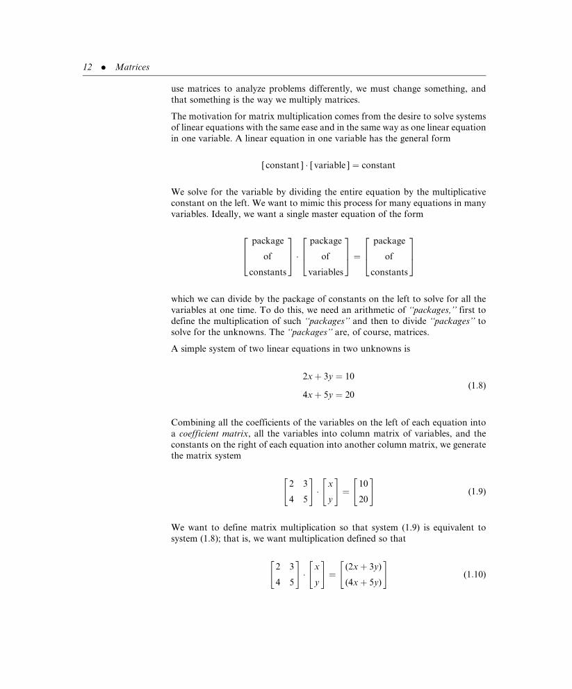
A simple system of two linear equations in two unknowns is
2xþ 3y ¼ 10
4xþ 5y ¼ 20(1:8)
Combining all the coefficients of the variables on the left of each equation into
a coefficient matrix, all the variables into column matrix of variables, and the
constants on the right of each equation into another column matrix, we generate
the matrix system
2 3
4 5
" #�
x
y
" #¼
10
20
" #(1:9)
We want to define matrix multiplication so that system (1.9) is equivalent to
system (1.8); that is, we want multiplication defined so that
2 3
4 5
" #�
x
y
" #¼
(2xþ 3y)
(4xþ 5y)
" #(1:10)
12 . Matrices

Then system (1.9) becomes
(2xþ 3y)
(4xþ 5y)
� �¼ 10
20
� �
which, from our definition of matrix equality, is equivalent to system (1.8).
We shall define the product AB of two matrices A and B when the number of
columns of A is equal to the number of rows of B, and the result will be a matrix
having the same number of rows as A and the same number of columns as B.
Thus, if A and B are
A ¼ 6 1 0
�1 2 1
� �and B ¼
�1 0 1 0
3 2 �2 1
4 1 1 0
24
35
then the product AB is defined, because A has three columns and B has three
rows. Furthermore, the product AB will be 2� 4 matrix, because A has two rows
and B has four columns. In contrast, the product BA is not defined, because the
number of columns in B is a different number from the number of rows in A.
A simple schematic for matrix multiplication is to write the orders of the matrices
to be multiplied next to each other in the sequence the multiplication is to be
done and then check whether the abutting numbers match. If the numbers
match, then the multiplication is defined and the order of the product matrix is
found by deleting the matching numbers and collapsing the two ‘‘�’’ symbols
into one. If the abutting numbers do not match, then the product is not defined.
In particular, if AB is to be found for A having order 2� 3 and B having order
3� 4, we write
(2� 3) (3� 4) (1:11)
where the abutting numbers are distinguished by the curved arrow. These
abutting numbers are equal, both are 3, hence the multiplication is defined.
Furthermore, by deleting the abutting threes in equation (1.11), we are left
with 2� 2, which is the order of the product AB. In contrast, the product BA
yields the schematic
(3� 4) (2� 3)
where we write the order of B before the order of A because that is the order of
the proposed multiplication. The abutting numbers are again distinguished by
the curved arrow, but here the abutting numbers are not equal, one is 4 and the
other is 2, so the product BA is not defined. In general, if A is an n� r matrix and
The product of two
matrices AB is
defined if the
number of columns
of A equals the
number of rows
of B.
1.2 Matrix Multiplication . 13

B is an r� p matrix, then the product AB is defined as an n� p matrix. The
schematic is
(n� r) (r� p) ¼ (n� p) (1:12)
When the product AB is considered, A is said to premultiply B while B is said to
postmultiply A.
Knowing the order of a product is helpful in calculating the product. If A and B
have the orders indicated in equation (1.12), so that the multiplication is defined,
we take as our motivation the multiplication in equation (1.10) and calculate the
i-j element (i ¼ 1, 2, . . . , n; j ¼ 1, 2, . . . , p) of the product AB ¼ C ¼ [cij] by multi-
plying the elements in the ith row of A by the corresponding elements in the jth
row column of B and summing the results. That is,
a11 a12 . . . a1k
a21 a22 . . . a2k
..
. ... ..
. ...
an1 an2 . . . ank
26664
37775
b11 b12 . . . b1p
b21 b22 . . . b2p
..
. ... ..
. ...
bk1 bk2 . . . bkp
26664
37775 ¼
c11 c12 . . . a1p
c21 c22 . . . c2p
..
. ... ..
. ...
cn1 cn2 . . . cnp
26664
37775
where
cij ¼ ai1b1j þ ai2b2j þ ai3b3j þ � � � þ airbrj ¼Xr
k¼1
aikbkj
In particular, c11 is obtained by multiplying the elements in the first row of A by
the corresponding elements in the first column of B and adding; hence
c11 ¼ a11b11 þ a12b21 þ a13b31 þ � � � þ a1rbr1
The element c12 is obtained by multiplying the elements in the first row of A by
the corresponding elements in the second column of B and adding; hence
c12 ¼ a11b12 þ a12b22 þ a13b32 þ � � � þ a1rbr2
The element c35, if it exists, is obtained by multiplying the elements in the third
row of A by the corresponding elements in the fifth column of B and adding;
hence
c35 ¼ a31b15 þ a32b25 þ a33b35 þ � � � þ a3rbr5
Example 1 Find AB and BA for
A ¼ 1 2 3
4 5 6
� �and B ¼
�7 �8
9 10
0 �11
24
35
To calculate the i-j
element of AB, when
the multiplication is
defined, multiply the
elements in the ith
row of A by the
corresponding
elements in the jth
column of B and
sum the results.
14 . Matrices

Solution: A has order 2� 3 and B has order 3� 2, so our schematic for the
product AB is
(2� 3) (3� 2)
The abutting numbers are both 3; hence the product AB is defined. Deleting both
abutting numbers, we have 2� 2 as the order of the product.
AB ¼1 2 3
4 5 6
� � �7 �8
9 10
0 �11
264
375
¼1(�7)þ 2(9)þ 3(0) 1(�8)þ 2(10)þ 3(�11)
4(�7)þ 5(9)þ 6(0) 4(�8)þ 5(10)þ 6(�11)
� �
¼11 �21
17 �48
� �
Our schematic for the product BA is
(3� 2) (2� 3)
The abutting numbers are now both 2; hence the product BA is defined. Deleting
both abutting numbers, we have 3� 3 as the order of the product BA.
BA ¼�7 �8
9 10
0 �11
264
375 1 2 3
4 5 6
� �
¼(�7)1þ (�8)4 (�7)2þ (�8)5 (�7)3þ (�8)6
9(1)þ 10(4) 9(2)þ 10(5) 9(3)þ 10(6)
0(1)þ (�11)4 0(2)þ (�11)5 0(3)þ (�11)6
264
375
¼�39 �54 �69
49 68 87
�44 �55 �66
264
375 &
Example 2 Find AB and BA for
A ¼2 1
�1 0
3 1
24
35 and B ¼ 3 1 5 �1
4 �2 1 0
� �
1.2 Matrix Multiplication . 15

Solution: A has two columns and B has two rows, so the product AB is defined.
AB ¼2 1
�1 0
3 1
264
375 3 1 5 �1
4 �2 1 0
� �
¼2(3)þ 1(4) 2(1)þ 1(�2) 2(5)þ 1(1) 2(�1)þ 1(0)
�1(3)þ 0(4) �1(1)þ 0(�2) �1(5)þ 0(1) �1(�1)þ 0(0)
3(3)þ 1(4) 3(1)þ 1(�2) 3(5)þ 1(1) 3(�1)þ 1(0)
264
375
¼10 0 11 �2
�3 �1 �5 1
13 1 16 �3
264
375
In contrast, B has four columns and A has three rows, so the product BA is not
defined. &
Observe from Examples 1 and 2 that AB 6¼ BA! In Example 1, AB is a 2� 2
matrix, whereas BA is a 3� 3 matrix. In Example 2, AB is a 3� 4 matrix, whereas
BA is not defined. In general, the product of two matrices is not commutative.
Example 3 Find AB and BA for
A ¼ 3 1
0 4
� �and B ¼ 1 1
0 2
� �
Solution:
AB ¼3 1
0 4
" #1 1
0 2
" #
¼3(1)þ 1(0) 3(1)þ 1(2)
0(1)þ 4(0) 0(1)þ 4(2)
" #
¼3 5
0 8
" #
BA ¼1 1
0 2
" #3 1
0 4
" #
¼1(3)þ 1(0) 1(1)þ 1(4)
0(3)þ 2(0) 0(1)þ 2(4)
" #
¼3 5
0 8
" #&
In general,
AB 6¼ BA.
16 . Matrices

In Example 3, the products AB and BA are defined and equal. Although matrix
multiplication is not commutative, as a general rule, some matrix products are
commutative. Matrix multiplication also lacks other familiar properties besides
commutivity. We know from our experiences with real numbers that if the
product ab ¼ 0, then either a ¼ 0 or b ¼ 0 or both are zero. This is not true, in
general, for matrices. Matrices exist for which AB ¼ 0 without either A or B
being zero (see Problems 20 and 21). The cancellation law also does not hold for
matrix multiplication. In general, the equation AB ¼ AC does not imply that
B ¼ C (see Problems 22 and 23). Matrix multiplication, however, does retain
some important properties.
" Theorem 1. If A, B, and C have appropriate orders so that the following
additions and multiplications are defined, then
(a) A(BC) ¼ (AB)C (associate law of multiplication)
(b) A(Bþ C) ¼ ABþ AC (left distributive law)
(c) (Bþ C)A ¼ BAþ CA (right distributive law) 3
Proof: We leave the proofs of parts (a) and (c) as exercises (see Problems 37
and 38). To prove part (b), we assume that A ¼ [aij ] is an m� n matrix and both
B ¼ [bij ] and C ¼ [cij ] are n� p matrices. Then
A(Bþ C) ¼ [aij] [bij]þ [cij ]� �
¼ [aij] (bij þ cij)� �
definition of matrix addition
¼Xn
k¼1
aik bkj þ ckj
�)
" #definition of matrix multiplication
¼Xn
k¼1
aikbkj þ aikckj
�)
" #
¼Xn
k¼1
aikbkj þXn
k¼1
aikckj
" #
¼Xn
k¼1
aikbkj
" #þ
Xn
k¼1
aikckj
" #definition of matrix addition
¼ [aij][bij]þ [aij ][cij ] definition of matrix multiplication &
1.2 Matrix Multiplication . 17

With multiplication defined as it is, we can decouple a system of linear equations
so that all of the variables in the system are packaged together. In particular, the
set of simultaneous linear equations
5x� 3yþ 2z ¼ 14
xþ y� 4z ¼ �7
7x�3z ¼ 1
(1:13)
can be written as the matrix equation Ax ¼ b where
A ¼5 �3 2
1 1 �4
7 0 �3
24
35, x ¼
x
y
z
2435, and b ¼
14
�7
1
24
35:
The column matrix x lists all the variables in equations (1.13), the column matrix
b enumerates the constants on the right sides of the equations in (1.13), and the
matrix A holds the coefficients of the variables. A is known as a coefficient matrix
and care must taken in constructing A to place all the x coefficients in the first
column, all the y coefficients in the second column, and all the z coefficients in
the third column. The zero in 3-2 location in A appears because the coefficient
of y in the third equation of (1.13) is zero. By redefining the matrices A, x, and
b appropriately, we can represent any system of simultaneous linear equations by
the matrix equation
Ax ¼ b (1:14)
Example 4 The system of linear equations
2xþ y� z ¼ 4
3xþ 2yþ 2w ¼ 0
x� 2yþ 3zþ 4w ¼ �1
has the matrix form Ax ¼ b with
A ¼2 1 �1 0
3 2 0 2
1 �2 3 4
24
35, x ¼
x
y
z
w
2664
3775, and b ¼
4
0
�1
24
35: &
We have accomplished part of the goal we set in the beginning of this section: to
write a system of simultaneous linear equations in the matrix form Ax ¼ b,
Any system of
simultaneous linear
equations can be
written as the matrix
equation Ax ¼ b.
18 . Matrices

where all the variables are segregated into the column matrix x. All that remains
is to develop a matrix operation to solve the matrix equation Ax ¼ b for x. To do
so, at least for a large class of square coefficient matrices, we first introduce some
additional matrix notation and review the traditional techniques for solving
systems of equations, because those techniques form the basis for the missing
matrix operation.
Problems 1.2
(1) Determine the orders of the following products if the order of A is 2� 4, the
order of B is 4� 2, the order of C is 4� 1, the order of D is 1� 2, and the order
of E is 4� 4.
(a) AB, (b) BA, (c) AC, (d) CA, (e) CD, (f ) AE,
(g) EB, (h) EA, (i) ABC, ( j) DAE, (k) EBA, (l) EECD.
In Problems 2 through 9, find the indicated products for
A ¼1 2
3 4
� �, B ¼
5 6
7 8
� �, C ¼
�1 0 1
3 �2 1
� �, D ¼
1 1
�1 2
2 �2
264
375,
E ¼�2 2 1
0 �2 �1
1 0 1
264
375, F ¼
0 1 2
�1 �1 0
1 2 3
264
375,
x ¼ [ 1 �2 ], y ¼ [ 1 2 1 ]:
(2) AB. (3) BA. (4) AC. (5) BC. (6) CB. (7) xA.
(8) xB. (9) xC. (10) Ax. (11) CD. (12) DC. (13) yD.
(14) yC. (15) Dx. (16) xD. (17) EF. (18) FE. (19) yF.
(20) Find AB for A ¼ 2 6
3 9
� �and B ¼ 3 �6
�1 2
� �. Note that AB ¼ 0 but neither A
nor B equals the zero matrix.
(21) Find AB for A ¼ 4 2
2 1
� �and B ¼ 3 �4
�6 8
� �.
(22) Find AB and AC for A ¼ 4 2
2 1
� �, B ¼ 1 1
2 1
� �, and C ¼ 2 2
0 �1
� �. What does
this result imply about the cancellation law for matrices?
(23) Find AB and CB for A ¼ 3 2
1 0
� �, B ¼ 2 4
1 2
� �, and C ¼ 1 6
3 �4
� �. Show that
AB ¼ CB but A 6¼ C.
(24) Calculate the product1 2
3 4
� �x
y
� �.
(25) Calculate the product
1 0 �1
3 1 1
1 3 0
24
35 x
y
z
2435.
1.2 Matrix Multiplication . 19

(26) Calculate the producta11 a12
a21 a22
� �x
y
� �.
(27) Calculate the productb11 b12 b13
b21 b22 b23
� � x
y
z
2435.
(28) Evaluate the expression A2 � 4A� 5I for the matrix A ¼ 1 2
4 3
� �.
(29) Evaluate the expression (A� I)(Aþ 2I) for the matrix A ¼ 3 5
�2 4
� �.
(30) Evaluate the expression (I� A)(A2 � I) for the matrix A ¼2 �1 1
3 �2 1
0 0 1
24
35.
(31) Use the definition of matrix multiplication to show that
jth column of (AB) ¼ A� ( jth column of B):
(32) Use the definition of matrix multiplication to show that
ith row of (AB) ¼ (ith row of A)� B:
(33) Prove that if A has a row of zeros and B is any matrix for which the product AB is
defined, then AB also has a row of zeros.
(34) Show by example that if B has a row of zeros and A is any matrix for which the
product AB is defined, then AB need not have a row of zeros.
(35) Prove that if B has a column of zeros and A is any matrix for which the product AB
is defined, then AB also has a column of zeros.
(36) Show by example that if A has a column of zeros and B is any matrix for which the
product AB is defined, then AB need not have a column of zeros.
(37) Prove part (a) of Theorem 1.
(38) Prove part (c) of Theorem 1.
In Problems 39 through 50, write each system in matrix form Ax ¼ b.
(39) 2xþ 3y ¼ 10 (40) 5xþ 20y ¼ 80
4x� 5y ¼ 11 �xþ 4y ¼ �64
(41) 3xþ 3y ¼ 100 (42) xþ 3y ¼ 4
6x� 8y ¼ 300 2x� y ¼ 1
�xþ 2y ¼ 500 �2x� 6y ¼ �8
4x� 9y ¼ �5
�6xþ 3y ¼ �3
(43) xþ y� z ¼ 0 (44) 2x� y ¼ 12
3xþ 2yþ 4z ¼ 0 �4y� z ¼ 15
20 . Matrices
(45) xþ 2y� 2z ¼ �1 (46) 2xþ y� z ¼ 0
2xþ yþ z ¼ 5 xþ 2yþ z ¼ 0
�xþ y� z ¼ �2 3x� yþ 2z ¼ 0
(47) xþ zþ y ¼ 2 (48) xþ 2y� z ¼ 5
3zþ 2xþ y ¼ 4 2x� yþ 2z ¼ 1
3yþ x ¼ 1 2xþ 2y� z ¼ 7
xþ 2yþ z ¼ 3
(49) 5xþ 3yþ 2zþ 4w ¼ 5 (50) 2x� yþ z� w ¼ 1
xþ yþ w ¼ 0 xþ 2y� zþ 2w ¼ �1
3xþ 2yþ 2z ¼ �3 x� 3yþ 2z� 3w ¼ 2
xþ yþ 2zþ 3w ¼ 4
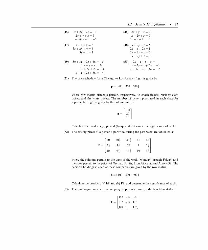
(51) The price schedule for a Chicago to Los Angeles flight is given by
p ¼ [ 200 350 500 ]
where row matrix elements pertain, respectively, to coach tickets, business-class
tickets and first-class tickets. The number of tickets purchased in each class for
a particular flight is given by the column matrix
n ¼130
20
10
24
35
Calculate the products (a) pn and (b) np, and determine the significance of each.
(52) The closing prices of a person’s portfolio during the past week are tabulated as
P ¼
40 40 12
40 78
41 41
3 14
3 58
3 12
4 3 78
10 9 34
10 18
10 9 58
2664
3775
where the columns pertain to the days of the week, Monday through Friday, and
the rows pertain to the prices of Orchard Fruits, Lion Airways, and Arrow Oil. The
person’s holdings in each of these companies are given by the row matrix
h ¼ [ 100 500 400 ]
Calculate the products (a) hP and (b) Ph, and determine the significance of each.
(53) The time requirements for a company to produce three products is tabulated in
T ¼0:2 0:5 0:4
1:2 2:3 1:7
0:8 3:1 1:2
264
375
1.2 Matrix Multiplication . 21

where the rows pertain to lamp bases, cabinets, and tables, respectively. The
columns pertain to the hours of labor required for cutting the wood, assembling,
and painting, respectively. The hourly wages of a carpenter to cut wood, of
a craftsperson to assemble a product, and of a decorator to paint are given,
respectively, by the columns of the matrix
w ¼10:50
14:00
12:25
24
35
Calculate the product Tw and determine its significance.
(54) Continuing with the information provided in the previous problem, assume further
that the number of items on order for lamp bases, cabinets, and tables, respectively,
are given in the rows of
q ¼ [ 1000 100 200 ]
Calculate the product qTw and determine its significance.
(55) The results of a flue epidemic at a college campus are collected in the matrix
F ¼0:20 0:20 0:15 0:15
0:10 0:30 0:30 0:40
0:70 0:50 0:55 0:45
24
35
where each element is a percent converted to a decimal. The columns pertain to
freshmen, sophomores, juniors, and seniors, respectively; whereas the rows repre-
sent bedridden students, students who are infected but ambulatory, and well
students, respectively. The male-female composition of each class is given by the
matrix
C ¼
1050 950
1100 1050
360 500
860 1000
2664
3775:
Calculate the product FC and determine its significance.
1.3 SPECIAL MATRICES
Certain types of matrices appear so frequently that it is advisable to discuss
them separately. The transpose of a matrix A, denoted by AT, is obtained by
converting all the rows of A into the columns of AT while preserving the ordering
of the rows/columns. The first row of A becomes the first column of AT, the
second row of A becomes the second column of AT, and the last row of A
becomes the last column of AT. More formally, if A ¼ [aij ] is an n� p matrix,
then the transpose of A, denoted by AT ¼ aTij
h i, is a p� n matrix where aT
ij ¼ aji.
The transpose A is
obtained by
converting all the
rows of A into
columns while
preserving the
ordering of the
rows/columns.
22 . Matrices
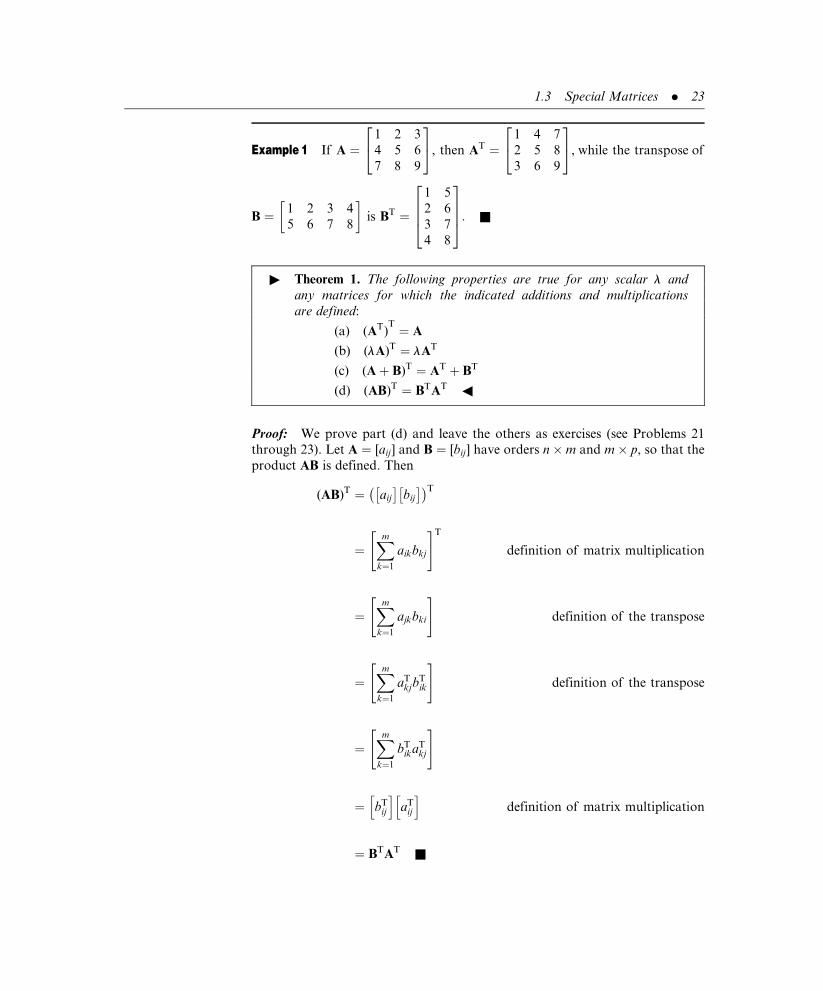
Example 1 If A ¼1 2 3
4 5 6
7 8 9
24
35, then AT ¼
1 4 7
2 5 8
3 6 9
24
35, while the transpose of
B ¼ 1 2 3 4
5 6 7 8
� �is BT ¼
1 5
2 6
3 7
4 8
2664
3775: &
" Theorem 1. The following properties are true for any scalar l and
any matrices for which the indicated additions and multiplications
are defined:
(a) (AT)T ¼ A
(b) (lA)T ¼ lAT
(c) (Aþ B)T ¼ AT þ BT
(d) (AB)T ¼ BTAT3
Proof: We prove part (d) and leave the others as exercises (see Problems 21
through 23). Let A ¼ [aij ] and B ¼ [bij] have orders n�m and m� p, so that the
product AB is defined. Then
(AB)T ¼ aij
� �bij
� �� �T
¼Xmk¼1
aikbkj
" #T
definition of matrix multiplication
¼Xmk¼1
ajkbki
" #definition of the transpose
¼Xmk¼1
aTkjb
Tik
" #definition of the transpose
¼Xmk¼1
bTika
Tkj
" #
¼ bTij
h iaT
ij
h idefinition of matrix multiplication
¼ BTAT&
1.3 Special Matrices . 23

Observation: The transpose of a product of matrices is not the product of the
transposes but rather the commuted product of the transposes.
A matrix A is symmetric if it equals its own transpose; that is, if A ¼ AT. A matrix
A is skew-symmetric if it equals the negative of its transpose; that is, if A ¼ �AT.
Example 2 A ¼1 2 3
2 4 5
3 5 6
24
35is symmetric while B ¼
0 2 �3
�2 0 1
3 �1 0
24
35 is
skew-symmetric. &
A submatrix of a matrix A is a matrix obtained from A by removing any number
of rows or columns from A. In particular, if
A ¼
1 2 3 4
5 6 7 8
9 10 11 12
13 14 15 16
2664
3775 (1:16)
then both B ¼ 10 12
14 16
� �and C ¼ [ 2 3 4 ] are submatrices of A. Here B is
obtained by removing the first and second rows together with the first and third
columns from A, while C is obtained by removing from A the second, third, and
fourth rows together with the first column. By removing no rows and no columns
from A, it follows that A is a submatrix of itself.
A matrix is partitioned if it is divided into submatrices by horizontal and vertical
lines between rows and columns. By varying the choices of where to place
the horizontal and vertical lines, one can partition a matrix in different ways.
Thus,
AB ¼ CGþDJ CH þDK
EGþ FJ EH þ FK
� �����
provided the partitioning was such that the indicated multiplications are
defined.
Example 3 Find AB if
A ¼
3 1 0
2 0 1
0 0 3
0 0 1
0 0 0
26666664
37777775 and B ¼
2 1 0 0 0
�1 1 0 0 0
0 1 0 0 1
264
375
�������
������������
A submatrix of a
matrix A is a matrix
obtained from A by
removing any
number of rows or
columns from A.
A matrix is
partitioned if it is
divided into
submatrices by
horizontal and
vertical lines
between rows and
columns.
24 . Matrices

Solution: From the indicated partitions, we find that
AB ¼
3 1
2 0
� �2 1
�1 1
� �þ
0
0
� �0 1½ �
3 1
2 0
� �0 0 0
0 0 0
� �þ
0
0
� �0 0 1½ �
0 0
0 0
� �2 1
�1 1
� �þ
3
1
� �0 1½ �
0 0
0 0
� �0 0 0
0 0 0
� �þ
3
1
� �0 0 1½ �
0 0½ �2 1
�1 1
� �þ 0½ � 0 1½ � 0 0½ �
0 0 0
0 0 0
� �þ 0½ � 0 0 1½ �
26666666664
37777777775
���������������
¼
5 4
4 2
� �þ
0 0
0 0
� �0 0 0
0 0 0
� �þ
0 0 0
0 0 0
� �5 4
4 2
� �þ
0 0
0 0
� �0 0 0
0 0 0
� �þ
0 0 0
0 0 0
� �
0 0½ � þ 0 0½ � 0 0 0½ � þ 0 0 0½ �
266666664
377777775
�������������
¼
5 4 0 0 0
4 2 0 0 0
0 3 0 0 3
0 1 0 0 1
0 0 0 0 0
26666664
37777775 ¼
5 4 0 0 0
4 2 0 0 0
0 3 0 0 3
0 1 0 0 1
0 0 0 0 0
266664
377775
������������Note that we partitioned to make maximum use of the zero submatrices of both
A and B. &
A zero row in a matrix is a row containing only zero elements, whereas a nonzero
row is a row that contains at least one nonzero element.
" Definition 1. A matrix is in row-reduced form if it satisfies the fol-
lowing four conditions:
(i) All zero rows appear below nonzero rows when both
types are present in the matrix.
(ii) The first nonzero element in any nonzero row is 1.
(iii) All elements directly below (that is, in the same column
but in succeeding rows from) the first nonzero element
of a nonzero row are zero.
(iv) The first nonzero element of any nonzero row appears
in a later column (further to the right) than the first
nonzero element in any preceding row.
"
Row-reducedmatricesare invaluable forsolvingsetsof simultaneous linearequations.
We shall use these matrices extensively in succeeding sections, but at present we are
interested only in determiningwhether a givenmatrix is or is not in row-reduced form.
1.3 Special Matrices . 25
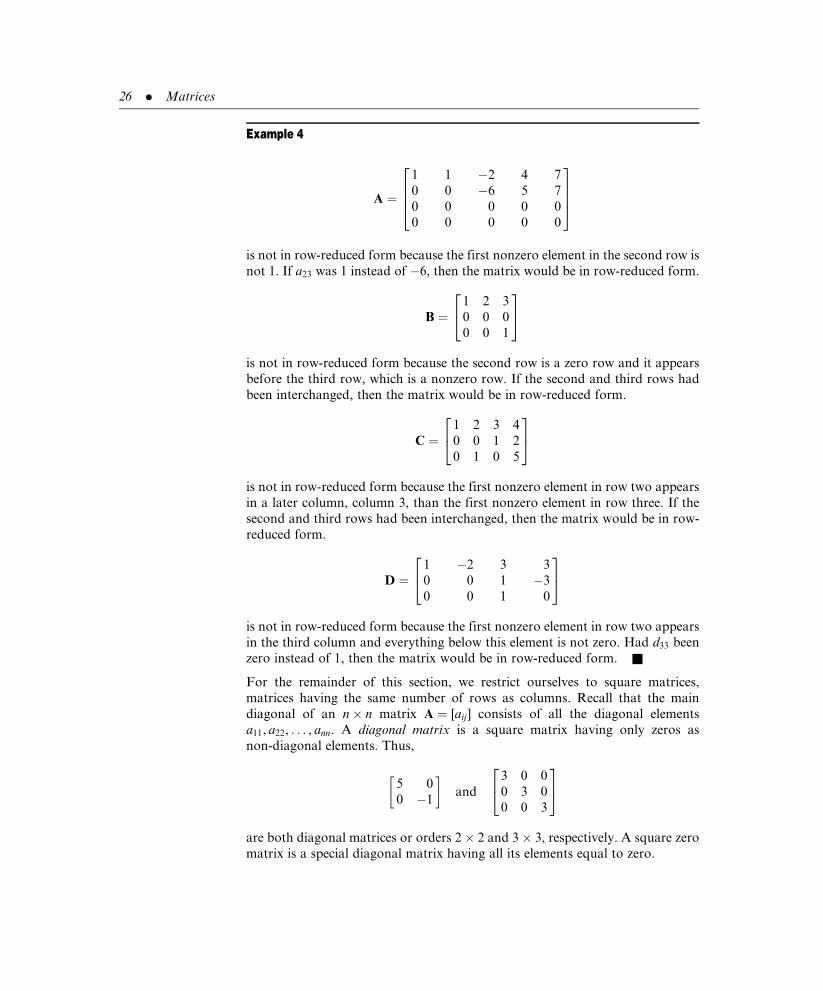
Example 4
A ¼
1 1 �2 4 7
0 0 �6 5 7
0 0 0 0 0
0 0 0 0 0
2664
3775
is not in row-reduced form because the first nonzero element in the second row is
not 1. If a23 was 1 instead of �6, then the matrix would be in row-reduced form.
B ¼1 2 3
0 0 0
0 0 1
24
35
is not in row-reduced form because the second row is a zero row and it appears
before the third row, which is a nonzero row. If the second and third rows had
been interchanged, then the matrix would be in row-reduced form.
C ¼1 2 3 4
0 0 1 2
0 1 0 5
24
35
is not in row-reduced form because the first nonzero element in row two appears
in a later column, column 3, than the first nonzero element in row three. If the
second and third rows had been interchanged, then the matrix would be in row-
reduced form.
D ¼1 �2 3 3
0 0 1 �3
0 0 1 0
24
35
is not in row-reduced form because the first nonzero element in row two appears
in the third column and everything below this element is not zero. Had d33 been
zero instead of 1, then the matrix would be in row-reduced form. &
For the remainder of this section, we restrict ourselves to square matrices,
matrices having the same number of rows as columns. Recall that the main
diagonal of an n� n matrix A ¼ [aij ] consists of all the diagonal elements
a11, a22, . . . , ann. A diagonal matrix is a square matrix having only zeros as
non-diagonal elements. Thus,
5 0
0 �1
� �and
3 0 0
0 3 0
0 0 3
24
35
are both diagonal matrices or orders 2� 2 and 3� 3, respectively. A square zero
matrix is a special diagonal matrix having all its elements equal to zero.
26 . Matrices

An identity matrix, denoted as I, is a diagonal matrix having all its diagonal
elements equal to 1. The 2� 2 and 4� 4 identity matrices are, respectively,
1 0
0 1
� �and
1 0 0 0
0 1 0 0
0 0 1 0
0 0 0 1
2664
3775
If A and I are square matrices of the same order, then
AI ¼ IA ¼ A: (1:17)
A block diagonal matrix A is one that can be partitioned into the form
A ¼
A1
A2 0A3
. ..
0 Ak
2666666664
3777777775
where A1, A2, . . . , Ak are square submatrices. Block diagonal matrices are par-
ticularly easy to multiply because in partitioned form they act as diagonal
matrices.
A matrix A ¼ [aij] is upper triangular if aij ¼ 0 for i > j; that is, if all elements
below the main diagonal are zero. If aij ¼ 0 for i < j, that is, if all elements above
the main diagonal are zero, then A is lower triangular. Examples of upper and
lower triangular matrices are, respectively,
�1 2 4 1
0 1 3 �1
0 0 2 5
0 0 0 5
2664
3775 and
5 0 0 0
�1 2 0 0
0 1 3 0
2 1 4 1
2664
3775
" Theorem 2. The product of two lower (upper) triangular matrices of
the same order is also lower (upper) triangular.
"
Proof: We prove this proposition for lower triangular matrices and leave the
upper triangular case as an exercise (see Problem 35). Let A ¼ [aij ] and B ¼ [bij]
both be n� n lower triangular matrices, and set AB ¼ C ¼ [cij]. We need to show
that C is lower triangular, or equivalently, that cij ¼ 0 when i < j. Now
cij ¼Xn
k¼1
aikbkj ¼Xj�1
k¼1
aikbkj þXn
k¼j
aikbkj
An identity matrix I
is a diagonal matrix
having all its
diagonal elements
equal to 1.
1.3 Special Matrices . 27

We are given that both A and B are lower triangular, hence aik ¼ 0 when i < k
and bkj ¼ 0 when k < j. Thus,
Xj�1
k¼1
aikbkj ¼Xj�1
k¼1
aik(0) ¼ 0
because in this summation k is always less than j. Furthermore, if we restrict
i < j, then
Xn
k¼j
aikbkj ¼Xn
k¼j
(0)bkj ¼ 0
because i < j � k. Thus, cij ¼ 0 when i < j. &
Finally, we define positive integral powers of matrix in the obvious manner:
A2 ¼ AA, A3 ¼ AAA ¼ AA2 and, in general, for any positive integer n
An ¼ AA . . . A|fflfflfflfflffl{zfflfflfflfflffl}n-times
(1:18)
For n ¼ 0, we define A0 ¼ I.
Example 5 If A ¼ 1 �2
1 3
� �, then A2 ¼ 1 �2
1 3
� �1 �2
1 3
� �¼ �1 �8
4 7
� �It follows directly from part (d) of Theorem 1 that
(A2)T ¼ (AA)T ¼ ATAT ¼ (AT)2,
which may be generalized to
(An)T ¼ (AT)n (1:19)
for any positive integer n. &
Problems 1.3
(1) For each of the following pairs of matrices A and B, find the products (AB)T,ATBT,
and BTAT and verify that (AB)T ¼ BTAT.
(a) A ¼ 3 0
4 1
� �, B ¼ �1 2 1
3 �1 0
� �.
(b) A ¼ 2 2 2
3 4 5
� �, B ¼
1 2
3 4
5 6
24
35.
(c) A ¼1 5 �1
2 1 3
0 7 �8
24
35, B ¼
6 1 3
2 0 �1
�1 �7 2
24
35.
28 . Matrices

(2) Verify that (Aþ B)T ¼ AT þ BT for the matrices given in part (c) of Problem 1.
(3) Find xTx and xxT for x ¼2
3
4
2435.
(4) Simplify the following expressions:
(a) (ABT)T
(b) (Aþ BT)T þ AT
(c) [AT(Bþ CT)]T
(d) [(AB)T þ C]T
(e) [(Aþ AT)(A� AT)]T:
(5) Which of the following matrices are submatrices of A ¼1 2 3
4 5 6
7 8 9
24
35?
(a)1 3
7 9
� �, (b) [1], (c)
1 2
8 9
� �, (d)
4 6
7 9
� �:
(6) Identify all of the nonempty submatrices of A ¼ a b
c d
� �.
(7) Partition A ¼
4 1 0 0
2 2 0 0
0 0 1 0
0 0 1 2
2664
3775 into block diagonal form and then calculate A2.
(8) Partition B ¼
3 2 0 0
�1 1 0 0
0 0 2 1
0 0 1 �1
2664
3775 into block diagonal form and then calculate B2.
(9) Use the matrices defined in Problems (7) and (8), partitioned into block diagonal
form, to calculate AB.
(10) Use partitioning to calculate A2 and A3 for
A ¼
1 0 0 0 0 0
0 2 0 0 0 0
0 0 0 1 0 0
0 0 0 0 1 0
0 0 0 0 0 1
0 0 0 0 0 0
26666664
37777775:
What is An for any positive integer n > 3?
(11) Determine which, if any, of the following matrices are in row-reduced form:
A ¼
0 1 0 4 �7
0 0 0 1 2
0 0 0 0 1
0 0 0 0 0
26664
37775, B ¼
1 1 0 4 �7
0 1 0 1 2
0 0 1 0 1
0 0 0 1 5
26664
37775,
1.3 Special Matrices . 29

C ¼
1 1 0 4 �7
0 1 0 1 2
0 0 0 0 1
0 0 0 1 5
2664
3775, D ¼
0 1 0 4 �7
0 0 0 0 0
0 0 0 0 1
0 0 0 0 0
2664
3775,
E ¼2 2 2
0 2 2
0 0 2
24
35, F ¼
0 0 0
0 0 0
0 0 0
24
35,
G ¼1 2 3
0 0 1
1 0 0
24
35, H ¼
0 0 0
0 1 0
0 0 0
24
35,
J ¼0 1 1
1 0 2
0 0 0
24
35, K ¼
1 0 2
0 �1 1
0 0 0
24
35,
L ¼2 0 0
0 2 0
0 0 0
24
35, M ¼
1 1=2 1=3
0 1 1=4
0 0 1
24
35,
N ¼1 0 0
0 0 1
0 0 0
24
35, Q ¼ 0 1
1 0
� �,
R ¼ 1 1
0 0
� �, S ¼ 1 0
1 0
� �,
T ¼ 1 12
0 1
� �:
(12) Determine which, if any, of the matrices in Problem 11 are upper triangular.
(13) Must a square matrix in row-reduced form necessarily be upper triangular?
(14) Must an upper triangular matrix be in row-reduced form?
(15) Can a matrix be both upper triangular and lower triangular simultaneously?
(16) Show that AB ¼ BA for
A ¼�1 0 0
0 3 0
0 0 1
24
35 and B ¼
5 0 0
0 3 0
0 0 2
24
35:
(17) Prove that if A and B are diagonal matrices of the same order, then AB ¼ BA.
(18) Does a 2� 2 diagonal matrix commute with every other 2� 2 matrix?
(19) Calculate the products AD and BD for
A ¼1 1 1
1 1 1
1 1 1
24
35, B ¼
0 1 2
3 4 5
6 7 8
24
35, and D ¼
2 0 0
0 3 0
0 0 �5
24
35:
What conclusions can you make about postmultiplying a square matrix by
a diagonal matrix?
30 . Matrices

(20) Calculate the products DA and DB for the matrices defined in Problem 19. What
conclusions can you make about premultiplying a square matrix by a diagonal
matrix?
(21) Prove that (AT)T ¼ A for any matrix A.
(22) Prove that (lA)T ¼ lAT for any matrix A and any scalar l.
(23) Prove that if A and B are matrices of the same order then (Aþ B)T ¼ AT þ BT.
(24) Let A, B, and C be matrices of orders m� p, p� r, and r� s, respectively. Prove
that (ABC)T ¼ CTBTAT.
(25) Prove that if A is a square matrix, then B ¼ (Aþ AT)=2 is a symmetric matrix.
(26) Prove that if A is a square matrix, then C ¼ (A� AT)=2 is a skew-symmetric matrix.
(27) Use the results of the last two problems to prove that any square matrix can be
written as the sum of a symmetric matrix and a skew-symmetric matrix.
(28) Write the matrix A in part (c) of Problem 1 as the sum of a symmetric matrix and
a skew-symmetric matrix.
(29) Write the matrix B in part (c) of Problem 1 as the sum of a symmetric matrix and
a skew-symmetric matrix.
(30) Prove that AAT is symmetric for any matrix A.
(31) Prove that the diagonal elements of a skew-symmetric matrix must be zero.
(32) Prove that if a 2� 2 matrix A commutes with every 2� 2 diagonal matrix, the A must
be diagonal. Hint: Consider, in particular, the diagonal matrix D ¼ 1 0
0 0
� �.
(33) Prove that if a n� n matrix A commutes with every n� n diagonal matrix, the
A must be diagonal.
(34) Prove that if D ¼ [dij ] is a diagonal matrix, then D ¼ d2ij
h i:
(35) Prove that the product of two upper triangular matrices is upper triangular.
1.4 LINEAR SYSTEMS OF EQUATIONS
Systems of simultaneous linear equations appear frequently in engineering and
scientific problems. The need for efficient methods that solve such systems was
one of the historical forces behind the introduction of matrices, and that need
continues today, especially for solution techniques that are applicable to large
systems containing hundreds of equations and hundreds of variables.
A system of m-linear equations in n-variables x1, x2, . . . , xn has the general form
a11x1 þ a12x2 þ . . .þ a1nxn ¼ b1
a21x1 þ a22x2 þ . . .þ a2nxn ¼ b2
..
.
am1x1 þ am2x2 þ . . .þ amnxn ¼ bm
(1:20)
1.4 Linear Systems of Equations . 31

where the coefficients aij (i ¼ 1, 2, . . . , m; j ¼ 1, 2, . . . , n) and the quantities bi
are all known scalars. The variables in a linear equation appear only to the first
power and are multiplied only by known scalars. Linear equations do not involve
products of variables, variables raised to powers other than one, or variables
appearing as arguments of transcendental functions.
For systems containing a few variables, it is common to denote the variables by
distinct letters such as x, y, and z. Such labeling is impractical for systems
involving hundreds of variables; instead a single letter identifies all variables
with different numerical subscripts used to distinguished different variables, such
as x1, x2, . . . , xn.
Example 1 The system
2xþ 3y� z ¼ 12,000
4x� 5yþ 6z ¼ 35,600
of two equations in the variables x, y, and z is linear, as is the system
20x1 þ 80x2 þ 35x3 þ 40x4 þ 55x5 ¼ �0:005
90x1 � 15x2 � 70x3 þ 25x4 þ 55x5 ¼ 0:015
30x1 þ 35x2 � 35x3 þ 10x4 � 65x5 ¼ �0:015
of three equations with five variables x1, x2, . . . , x5. In contrast, the system
2xþ 3xy ¼ 25
4ffiffiffixpþ sin y ¼ 50
is not linear for many reasons: it contains a product xy of variables; it contains
the variable x raised to the one-half power; and it contains the variable y as the
argument of the transcendental sine function. &
As shown in Section 1.2, any linear system of form (1.20) can be rewritten in the
matrix form
Ax ¼ b (1:14 repeated)
with
A ¼
a11 a12 . . . a1n
a21 a22 . . . a2n
..
. ... . .
. ...
am1 am2 . . . amn
266664
377775, x ¼
x1
x2
..
.
xn
266664
377775, and b ¼
b1
b2
..
.
bm
266664
377775:
32 . Matrices

If m 6¼ n, then A is not square and the dimensions of x and b will be different.
A solution to linear system (1.20) is a set of scalar values for the variables
x1, x2, . . . , xn that when substituted into each equation of the system makes
each equation true.
Example 2 The scalar values x ¼ 2 and y ¼ 3 are a solution to the system
3xþ 2y ¼ 12
6xþ 4y ¼ 24
A second solution is x ¼ �4 and y ¼ 12. In contrast, the scalar values
x ¼ 1, y ¼ 2, and z ¼ 3 are not a solution to the system
2xþ 3yþ 4z ¼ 20
4xþ 5yþ 6z ¼ 32
7xþ 8yþ 9z ¼ 40
because these values do not make the third equation true, even though they do
satisfy the first two equations of the system. &
" Theorem 1. If x1 and x2 are two different solutions of Ax ¼ b,
then z ¼ ax1 þ bx2 is also a solution for any real numbers a and b
with aþ b ¼ 1.
"
Proof: x1 and x2 are given as solutions of Ax ¼ b, hence Ax1 ¼ b, and
Ax2 ¼ b. Then
Az ¼ A(ax1 þ bx2) ¼ a(Ax1)þ b(Ax2) ¼ abþ bb ¼ (aþ b)b ¼ b,
so z is also a solution. &
Because there are infinitely many ways to form aþ b ¼ 1 (let a be any real
number and set b ¼ 1� a), it follows from Theorem 1 that once we identify two
solutions we can combine them into infinitely many other solutions. Conse-
quently, the number of possible solutions to a system of linear equations is either
none, one, or infinitely many.
The graph of a linear equation in two variables is a line in the plane; hence
a system of linear equations in two variables is depicted graphically by a set of
lines. A solution to such a system is a set of coordinates for a point in the plane
that lies on all the lines defined by the equations. In particular, the graphs of the
equations in the system
A solution to linear
system of equations
is a set of scalar
values for the
variables that when
substituted into
each equation of the
system makes each
equation true.
1.4 Linear Systems of Equations . 33

xþ y ¼ 1
x� y ¼ 0(1:21)
are shown in Figure 1.3. There is only one point of intersection, and the
coordinates of this point x ¼ y ¼ 12
is the unique solution to System (1.21). In
contrast, the graphs of the equations in the system
xþ y ¼ 1
xþ y ¼ 2(1:22)
are shown in Figure 1.4. The lines are parallel and have no points of intersection,
so System (1.22) has no solution. Finally, the graphs of the equations in the
system
xþ y ¼ 0
2xþ 2y ¼ 0(1:23)
Figure 1.3
4
3
3
x + y = 1
x − y = 0
2
2
1
1x
y
(1/2, 1/2)
−3 −2
−2
−1−1
Figure 1.4
4
3
3
x + y = 1
x + y = 2
2
2
1
1x
y
−3 −2
−2
−1−1
34 . Matrices

are shown in Figure 1.5. The lines overlap, hence every point on either line is
a point of intersection and System (1.23) has infinitely many solutions.
A system of simultaneous linear equations is consistent if it possesses at least one
solution. If no solution exists, the system is inconsistent. Systems (1.21) and (1.23)
are consistent; System (1.22) in inconsistent.
The graph of a linear equation in three variables is a plane in space; hence
a system of linear equations in three variables is depicted graphically by a set
of planes. A solution to such a system is the set of coordinates for a point in
space that lies on all the planes defined by the equations. Such a system can have
no solutions, one solution, or infinitely many solutions.
Figure 1.6 shows three planes that intersect at a single point, and it represents
a system of three linear equations in three variables with a unique solution.
Figures 1.7 and 1.8 show systems of planes that have no points that lie on all
three planes; each figure depicts a different system of three linear equations in
three unknowns with no solutions. Figure 1.9 shows three planes intersecting at
a line, and it represents a system of three equations in three variables with
infinitely many solutions, one solution corresponding to each point on the line.
A different example of infinitely many solutions is obtained by collapsing the
Figure 1.5
4
3
3
x + y = 0
2x + 2y = 0
2
2
1
1x
y
−3 −2
−2
−1−1
Figure 1.6
1.4 Linear Systems of Equations . 35

three planes in Figure 1.7 onto each other so that each plane is an exact copy of
the others. Then every point on one plane is also on the other two.
System (1.20) is homogeneous if the right side of each equation is 0; that is, if
b1 ¼ b2 ¼ . . . ¼ bm ¼ 0. In matrix form, we say that the system Ax ¼ b is homo-
geneous if b ¼ 0, a zero column matrix. If b 6¼ 0, which implies that at least one
component of b differs from 0, then the system of equations is nonhomogeneous.
System (1.23) is homogeneous; Systems (1.21) and (1.22) are nonhomogeneous.
One solution to a homogeneous system of equations is obtained by setting all
variables equal to 0. This solution is called the trivial solution. Thus, we have the
following theorem.
Figure 1.7
Figure 1.8
Figure 1.9
A homogeneous
system of linear
equations has the
matrix form Ax ¼ 0;
one solution is the
trivial solution
x ¼ 0.
36 . Matrices

" Theorem 2. A homogeneous system of linear equations is
consistent.
"
All the scalars contained in the system of equations Ax ¼ b appear in the
coefficient matrix A and the column matrix b. These scalars can be combined
into the single partitioned matrix [Ajb], known as the augmented matrix for the
system of equations.
Example 3 The system
x1 þ x2 � 2x3 ¼ �3
2x1 þ 5x2 þ 3x3 ¼ 11
�x1 þ 3x2 þ x3 ¼ 5
can be written as the matrix equation
1 1 �2
2 5 3
�1 3 1
24
35 x1
x2
x3
24
35 ¼ �3
11
5
24
35
which has as its augmented matrix
[Ajb] ¼1 1 �2
2 5 3
�1 3 1
�3
11
5
������24
35: &
Example 4 Write the set of equation in x, y, and z associated with the
augmented matrix
[Ajb] ¼ �2 1 3
0 4 5
8
�3
����� �
Solution:
�2xþ yþ 3z ¼ 8
4yþ 5z ¼ �3&
The traditional approach to solving a system of linear equations is to manipulate
the equations so that the resulting equations are easy to solve and have the
The augmented
matrix for Ax ¼ b
is the partitioned
matrix [Ajb].
1.4 Linear Systems of Equations . 37
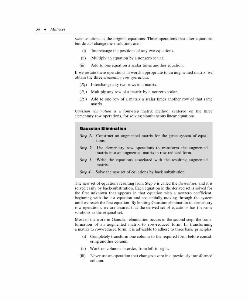
same solutions as the original equations. Three operations that alter equations
but do not change their solutions are:
(i) Interchange the positions of any two equations.
(ii) Multiply an equation by a nonzero scalar.
(iii) Add to one equation a scalar times another equation.
If we restate these operations in words appropriate to an augmented matrix, we
obtain the three elementary row operations:
(R1) Interchange any two rows in a matrix.
(R2) Multiply any row of a matrix by a nonzero scalar.
(R3) Add to one row of a matrix a scalar times another row of that same
matrix.
Gaussian elimination is a four-step matrix method, centered on the three
elementary row operations, for solving simultaneous linear equations.
The new set of equations resulting from Step 3 is called the derived set, and it is
solved easily by back-substitution. Each equation in the derived set is solved for
the first unknown that appears in that equation with a nonzero coefficient,
beginning with the last equation and sequentially moving through the system
until we reach the first equation. By limiting Gaussian elimination to elementary
row operations, we are assured that the derived set of equations has the same
solutions as the original set.
Most of the work in Gaussian elimination occurs in the second step: the trans-
formation of an augmented matrix to row-reduced form. In transforming
a matrix to row-reduced form, it is advisable to adhere to three basic principles:
(i) Completely transform one column to the required form before consid-
ering another column.
(ii) Work on columns in order, from left to right.
(iii) Never use an operation that changes a zero in a previously transformed
column.
Gaussian Elimination
Step 1. Construct an augmented matrix for the given system of equa-
tions.
Step 2. Use elementary row operations to transform the augmented
matrix into an augmented matrix in row-reduced form.
Step 3. Write the equations associated with the resulting augmented
matrix.
Step 4. Solve the new set of equations by back substitution.
38 . Matrices

Example 5 Use Gaussian elimination to solve the system
xþ 3y ¼ 4,
2x� y ¼ 1,
3xþ 2y ¼ 5,
5xþ 15y ¼ 20:
Solution: The augmented matrix for this system is
1 3
2 �1
3 2
5 15
4
1
5
20
��������2664
3775
We transform this augmented matrix into row-reduced form using only the three
elementary row operations. The first nonzero element in the first row appears in
the 1-1 position, so use elementary row operation R3 to transform all other
elements in the first column to zero.
1 3
2 �1
3 2
5 15
4
1
5
20
��������2664
3775!
1 3
0 �7
3 2
5 15
4
�7
5
20
��������2664
3775
by adding to the
second row �2
times the first row
!
1 3
0 �7
0 �7
5 15
4
�7
�7
20
��������2664
3775
by adding to the
third row �3
times the first row
!
1 3
0 �7
0 �7
0 0
4
�7
�7
0
��������2664
3775
by adding to the
fourth row �5
times the first row
The first row and the first column are correctly formatted, so we turn our
attention to the second row and second column. We use elementary row oper-
ations on the current augmented matrix to transform the first nonzero element in
the second row to one and then all elements under it, in the second column, to
zero. Thus,
1.4 Linear Systems of Equations . 39

!
1 3
0 1
0 �7
0 0
4
1
�7
0
����������
266664
377775
by multiplying thesecond row by� 1=7
!
1 3
0 1
0 0
0 0
4
1
0
0
����������
266664
377775
by adding to thethird row 7 timesthe second row
This augmented matrix is in row-reduced form, and the system of equations
associated with it is the derived set
xþ 3y ¼ 4
y ¼ 1
0 ¼ 0
0 ¼ 0:
Solving the second equation for y and then the first equation for x, we obtain
x ¼ 1 and y ¼ 1 as the solution to both this last set of equations and also the
original set of equations. &
When one element in a matrix is used to convert another element to zero by
elementary row operation R3, the first element is called a pivot. In Example 5,
we used the element in the 1-1 position first to cancel the element in the 2-1
position and then to cancel the elements in the 3-1 and 4-1 positions. In each
case, the unity element in the 1-1 position was the pivot. Later, we used the
unity element in the 2-2 position to cancel the element �7 in the 3-2 position;
here, the 2-2 element served as the pivot. We shall always use elementary row
operation R2 to transform a pivot to unity before using the pivot to transform
other elements to zero.
Example 6 Use Gaussian elimination to solve the system
xþ 2yþ z ¼ 3,
2xþ 3y� z ¼ �6,
3x� 2y� 4z ¼ �2:
A pivot is
transformed to
unity prior to using
it to cancel other
elements to zero.
40 . Matrices

Solution: Transforming the augmented matrix for this system into row-reduced
form using only elementary row operations, we obtain
1 2 1
2 3 �1
3 �2 �4
3
�6
�2
�������264
375!
1 2 1
0 �1 �3
3 �2 �4
3
�12
�2
�������264
375
by adding tothe second row �2times the first row
!1 2 1
0 �1 �3
0 �8 �7
3
�12
�11
�������264
375
by adding tothe third row �3times the first row
!1 2 1
0 1 3
0 �8 �7
3
12
�11
�������264
375
by multiplying thesecond row by� 1
!1 2 1
0 1 3
0 0 17
3
12
85
�������264
375
by adding to thethird row 8 timesthe second row
!1 2 1
0 1 3
0 0 1
3
12
5
�������264
375
by multiplying thethird row by 1=17
This augmented matrix is in row-reduced form; the derived set is
xþ 2yþ z ¼ 3
yþ 3z ¼ 12
z ¼ 5
Solving the third equation for z, then the second equation for y, and lastly, the
first equation for x, we obtain x ¼ 4, y ¼ �3, and z ¼ 5 as the solution to both
this last system and the original system of equations. &
Elementary row operation R1 is used to move potential pivots into more useful
locations by rearranging the positions of rows.
Example 7
Use Gaussian elimination to solve the system
2x3 þ 3x4 ¼ 0
x1 þ 3x3 þ x4 ¼ 0
x1 þ x2 þ 2x3 ¼ 0
1.4 Linear Systems of Equations . 41

Solution: The augmented matrix for this system is
0 0 2 3
1 0 3 1
1 1 2 0
0
0
0
������24
35
Normally, we would use the element in the 1-1 position to transform to zero the
two elements directly below it, but we cannot because the 1-1 element is itself
zero. To move a nonzero element into the ideal pivot position, we interchange
the first row with either of the other two rows. The choice is arbitrary.
0 0 2 3
1 0 3 1
1 1 2 0
0
0
0
��������2664
3775!
1 0 3 1
0 0 2 3
1 1 2 0
0
0
0
��������2664
3775
by interchanging the
first and second rows
!1 0 3 1
0 0 2 3
0 1 �1 �1
0
0
0
�������264
375
by adding to thethird row� 1 timesthe first row
!1 0 3 1
0 1 �1 �1
0 0 2 3
0
0
0
�������264
375
by interchanging thesecond and third rows
!1 0 3 1
0 1 �1 �1
0 0 1 3=2
0
0
0
�������264
375
by multiplying thethird row by 1=2
This augmented matrix is in row-reduced form; the derived set is
x1 þ 3x3 þ x4 ¼ 0
x2 � x3 � x4 ¼ 0
x3 þ 32x4 ¼ 0
We use the third equation to solve for x3, then the second equation to solve for
x2, and lastly, the first equation to solve for x1, because in each case those are the
variables that appear first in the respective equations. There is no defining
equation for x4, so this variable remains arbitrary, and we solve for the other
variables in terms of it. The solution to both this last set of equations and the
original set of equations is x1 ¼ (7=2)x4, x2 ¼ (� 1=2)x4 and x3 ¼ (� 3=2)x4
with x4 arbitrary. The solution can be written as the column matrix
x ¼
x1
x2
x3
x4
266664
377775 ¼
(7=2)x4
(� 1=2)x4
(� 3=2)x4
x4
266664
377775 ¼ x4
2
7
�1
�3
2
266664
377775 &
If the solution to a
derived set involves
at least one
arbitrary unknown,
then the original
system has infinitely
many solutions.
42 . Matrices

Example 7 is a system of equations with infinitely many solutions, one for each
real number assigned to the arbitrary variable x4. Infinitely many solutions
occur when the derived set of equations is consistent and has more unknowns
than equations. If a derived set contains n variables and r equations, n > r, then
each equation in the derived set is solved for the first variable in that equation
with a nonzero coefficient; this defines r variables and leaves the remaining n� r
variables as arbitrary. These arbitrary variables may be chosen in infinitely many
ways to produce solutions.
A homogeneous set of linear equations is always consistent. If such a system
has more variables than equations, then its derived set will also have more
variables than equations, resulting in infinitely many solutions. Thus, we have
the following important result:
" Theorem 3. A homogeneous system of linear equations containing
more variables than equations has infinitely many solutions.
"
In contrast to homogeneous systems, a nonhomogeneous system may have no
solutions. If a derived set of equations contains a false equation, such as 0 ¼ 1,
that set is inconsistent because no values for the variables can make the false
equation true. Because the derived set has the same solutions as the original set,
it follows that the original set is also inconsistent.
Example 8 Use Gaussian elimination to solve the system
xþ 2y ¼ 2,
3xþ 6y ¼ 7:
Solution: Transforming the augmented matrix for this system into row-reduced
form, we obtain
1 2
3 6
2
7
����� �
! 1 2
0 0
2
1
����� �
by adding the second row
�3 times the first row
This augmented matrix is in row-reduced form; the derived set is
xþ 2y ¼ 2
0 ¼ 1
No values of x and y can make this last equation true, so the derived set, as well
as the original set of equations, has no solution. &
If a derived set
contains a false
equation, then the
original set of
equations has no
solution.
1.4 Linear Systems of Equations . 43

Finally, we note that most augmented matrices can be transformed into a variety
of row-reduced forms. If a row-reduced augmented matrix has two nonzero
rows, then a different row-reduced augmented matrix is easily constructed by
adding to the first row any nonzero constant times the second row. The equa-
tions associated with both augmented matrices, different as they may be, will
have identical solutions.
Problems 1.4
(1) Determine whether the proposed values of x, y, and z are solutions to:
xþ yþ 2z ¼ 2,
x� y� 2z ¼ 0,
xþ 2yþ 2z ¼ 1:
(a) x ¼ 1, y ¼ �3, z ¼ 2. (b) x ¼ 1, y ¼ �1, z ¼ 1.
(2) Determine whether the proposed values of x1, x2, and x3 are solutions to:
x1 þ 2x2 þ 3x3 ¼ 6,
x1 � 3x2 þ 2x3 ¼ 0,
3x1 � 4x2 þ 7x3 ¼ 6:
(a) x1 ¼ 1, x2 ¼ 1, x3 ¼ 1:
(b) x1 ¼ 2, x2 ¼ 2, x3 ¼ 0:
(c) x1 ¼ 14, x2 ¼ 2, x3 ¼ �4:
(3) Find a value for k such that x ¼ 2 and y ¼ k is a solution of the system
3xþ 5y ¼ 11,
2x� 7y ¼ �3:
(4) Find a value for k such that x ¼ 2k, y ¼ �k, and z ¼ 0 is a solution of the system
xþ 2yþ z ¼ 0,
�2x� 4yþ 2z ¼ 0,
3x� 6y� 4z ¼ 1:
44 . Matrices
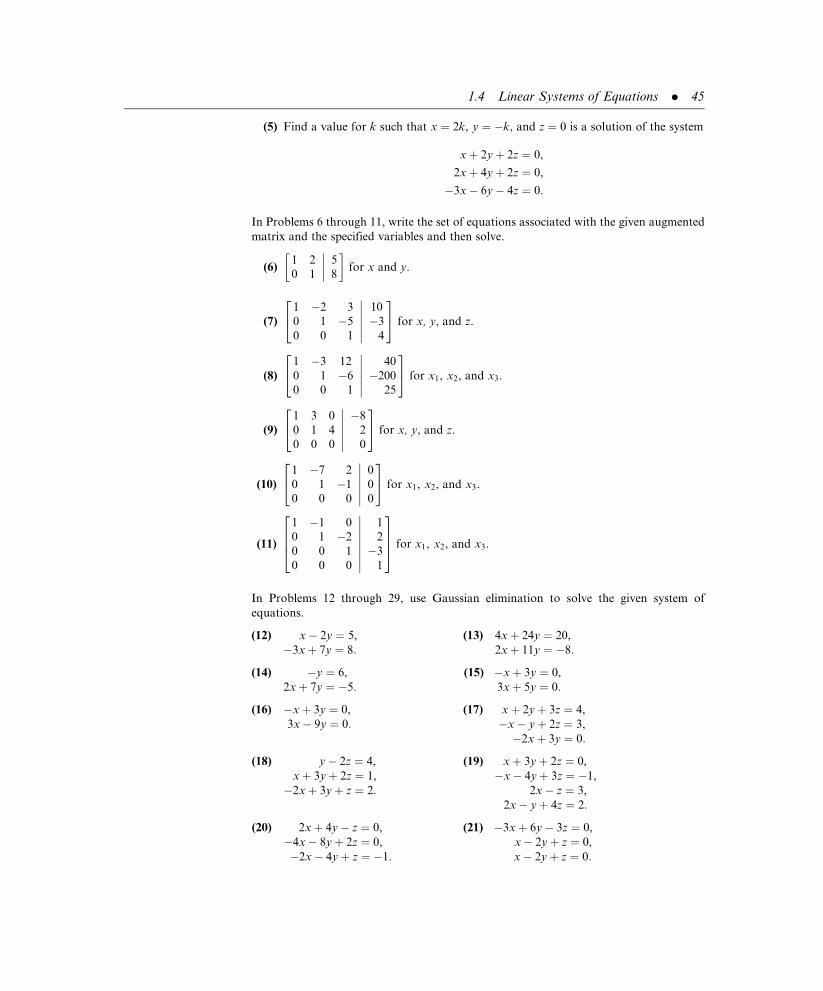
(5) Find a value for k such that x ¼ 2k, y ¼ �k, and z ¼ 0 is a solution of the system
xþ 2yþ 2z ¼ 0,
2xþ 4yþ 2z ¼ 0,
�3x� 6y� 4z ¼ 0:
In Problems 6 through 11, write the set of equations associated with the given augmented
matrix and the specified variables and then solve.
(6)1 2
0 1
5
8
����� �
for x and y.
(7)
1 �2 3
0 1 �5
0 0 1
10
�3
4
������24
35 for x, y, and z.
(8)
1 �3 12
0 1 �6
0 0 1
40
�200
25
������24
35 for x1, x2, and x3.
(9)
1 3 0
0 1 4
0 0 0
�8
2
0
������24
35 for x, y, and z.
(10)
1 �7 2
0 1 �1
0 0 0
0
0
0
������24
35 for x1, x2, and x3.
(11)
1 �1 0
0 1 �2
0 0 1
0 0 0
1
2
�3
1
��������2664
3775 for x1, x2, and x3.
In Problems 12 through 29, use Gaussian elimination to solve the given system of
equations.
(12) x� 2y ¼ 5, (13) 4xþ 24y ¼ 20,
�3xþ 7y ¼ 8: 2xþ 11y ¼ �8:
(14) �y ¼ 6, (15) �xþ 3y ¼ 0,
2xþ 7y ¼ �5: 3xþ 5y ¼ 0:
(16) �xþ 3y ¼ 0, (17) xþ 2yþ 3z ¼ 4,
3x� 9y ¼ 0: �x� yþ 2z ¼ 3,
�2xþ 3y ¼ 0:
(18) y� 2z ¼ 4, (19) xþ 3yþ 2z ¼ 0,
xþ 3yþ 2z ¼ 1, �x� 4yþ 3z ¼ �1,
�2xþ 3yþ z ¼ 2: 2x� z ¼ 3,
2x� yþ 4z ¼ 2:
(20) 2xþ 4y� z ¼ 0, (21) �3xþ 6y� 3z ¼ 0,
�4x� 8yþ 2z ¼ 0, x� 2yþ z ¼ 0,
�2x� 4yþ z ¼ �1: x� 2yþ z ¼ 0:
1.4 Linear Systems of Equations . 45

(22) �3xþ 3y� 3z ¼ 0, (23) �3x1 þ 6x2 � 3x3 ¼ 0,
x� yþ 2z ¼ 0, x1 � x2 þ x3 ¼ 0:2x� 2yþ z ¼ 0,
xþ yþ z ¼ 0:
(24) x1 � x2 þ 2x3 ¼ 0, (25) x1 þ 2x2 ¼ �3,
2x1 � 2x2 þ 4x3 ¼ 0: 3x1 þ x2 ¼ 1:
(26) x1 þ 2x2 � x3 ¼ �1, (27) x1 þ 2x2 ¼ 5,
2x1 � 3x2 þ 2x3 ¼ 4: �3x1 þ x2 ¼ 13,
4x1 þ 3x2 ¼ 0:
(28) 2x1 þ 4x2 ¼ 2, (29) 2x1 þ 3x2 � 4x3 ¼ 2,
3x1 þ 2x2 þ x3 ¼ 8, 3x1 � 2x2 ¼ �1,
5x1 � 3x2 þ 7x3 ¼ 15: 8x1 � x2 � 4x3 ¼ 10:
(30) Show graphically that the number of solutions to a linear system of two equations
in three variables is either none or infinitely many.
(31) Let y be a solution to Ax ¼ b and let z be a solution to the associated homogeneous
system Ax ¼ 0. Prove that u ¼ yþ z is also a solution to Ax ¼ b.
(32) Let y and z be as defined in Problem 31.
(a) For what scalars a is u ¼ yþ az also a solution to Ax ¼ b?
(b) For what scalars a is u ¼ ayþ z also a solution to Ax ¼ b?
In Problems 33 through 40, establish a set of equations that models each process
and then solve.
(33) A manufacturer receives daily shipments of 70,000 springs and 45,000 pounds of
stuffing for producing regular and support mattresses. Regular mattresses r require
50 springs and 30 pounds of stuffing; support mattresses s require 60 springs and 40
pounds of stuffing. How many mattresses of each type should be produced daily to
utilize all available inventory?
(34) A manufacturer produces desks and bookcases. Desks d require 5 hours of cutting
time and 10 hours of assembling time. Bookcases b require 15 minutes of cutting
time and 1 hour of assembling time. Each day the manufacturer has available
200 hours for cutting and 500 hours for assembling. How many desks and
bookcases should be scheduled for completion each day to utilize all available
workpower?
(35) A mining company has a contract to supply 70,000 tons of low-grade ore, 181,000
tons of medium-grade ore, and 41,000 tons of high-grade ore to a supplier. The
company has three mines that it can work. Mine A produces 8,000 tons of
low-grade ore, 5,000 tons of medium-grade ore, and 1,000 tons of high-grade ore
during each day of operation. Mine B produces 3,000 tons of low-grade ore, 12,000
tons of medium-grade ore, and 3,000 tons of high-grade ore for each day it is in
operation. The figures for mine C are 1,000, 10,000, and 2,000, respectively. How
many days must each mine operate to meet contractual demands without producing
a surplus?
(36) A small company computes its end-of-the- year bonus b as 5% of the net profit after
city and state taxes have been paid. The city tax c is 2% of taxable income, while the
state tax s is 3% of taxable income with credit allowed for the city tax as a pretax
deduction. This year, taxable income was $400,000. What is the bonus?
46 . Matrices

(37) A gasoline producer has $800,000 in fixed annual costs and incurs an additional
variable cost of $30 per barrel B of gasoline. The total cost C is the sum of the fixed
and variable costs. The net sales S is computed on a wholesale price of $40 per
barrel.
(a) Show that C, B, and S are related by two simultaneous equations.
(b) How many barrels must be produced to break even, that is, for net sales to
equal cost?
(38) (Leontief Closed Models) A closed economic model involves a society in which all
the goods and services produced by members of the society are consumed by those
members. No goods and services are imported from without and none are exported.
Such a system involves N members, each of whom produces goods or services
and charges for their use. The problem is to determine the prices each member
should charge for his or her labor so that everyone breaks even after one year. For
simplicity, it is assumed that each member produces one unit per year.
Consider a simple closed system limited to a farmer, a carpenter, and a weaver.
The farmer produces one unit of food each year, the carpenter produces one unit of
finished wood products each year, and the weaver produces one unit of clothing
each year. Let p1 denote the farmer’s annual income (that is, the price she charges
for her unit of food), let p2 denote the carpenter’s annual income (that is, the price
he charges for his unit of finished wood products), and let p3 denote the weaver’s
annual income. Assume on an annual basis that the farmer and the carpenter
consume 40% each of the available food, while the weaver eats the remaining
20%. Assume that the carpenter uses 25% of the wood products he makes, while
the farmer uses 30% and the weaver uses 45%. Assume further that the farmer uses
50% of the weaver’s clothing while the carpenter uses 35% and the weaver consumes
the remaining 15%. Show that a break-even equation for the farmer is
0:40p1 þ 0:30p2 þ 0:50p3 ¼ p1
while the break-even equation for the carpenter is
0:40p1 þ 0:25p2 þ 0:35p3 ¼ p2
What is the break-even equation for the weaver? Rewrite all three equations as
a homogeneous system and then find the annual incomes of each sector.
(39) Paul, Jim, and Mary decide to help each other build houses. Paul will spend half his
timeonhis ownhouse andaquarter of his timeon eachof the houses of JimandMary.
Jim will spend one third of his time on each of the three houses under construction.
Mary will spend one sixth of her time on Paul’s house, one third on Jim’s house, and
onehalf of her timeonher ownhouse. For tax purposes, eachmust place a price on his
or her labor, but they want to do so in a way that each will break-even. Show that the
process of determining break-even wages is a Leontief closed model containing three
homogeneous equations and then find the wages of each person.
(40) Four third-world countries each grow a different fruit for export and each uses the
income from that fruit to pay for imports of the fruits from the other countries.
Country A exports 20% of its fruit to country B, 30% to country C, 35% to country
D, and uses the rest of its fruit for internal consumption. Country B exports 10% of
its fruit to country A, 15% to country C, 35% to country D, and retains the rest for
its own citizens. Country C does not export to country A; it divides its crop equally
1.4 Linear Systems of Equations . 47

between countries B and D and its own people. Country D does not consume its
own fruit; all is for export with 15% going to country A, 40% to country C, and 45%
to country D. Show that the problem of determining prices on the annual harvests
of fruit so that each country breaks even is equivalent to solving four homogeneous
equations in four unknowns and then find the prices.
Gaussian elimination is often programmed for computer implementation, but
because all computers store numbers as a finite string of digits, round-off error
can be significant. A popular strategy for minimizing round-off errors is partial
pivoting, which requires that a pivot always be larger than or equal in absolute value
than any element below the pivot in the same column. This is accomplished by using
elementary row operation R1 to interchange rows whenever necessary. In Problems
41 through 46, determine the first pivot under a partial pivoting strategy for the
given augmented matrix.
(41)1 3
4 8
35
15
����� �
(42)1 �2
5 3
�5
85
����� �
(43)
�2 8 �3
4 5 4
�3 �1 2
100
75
250
������24
35 (44)
1 2 3
5 6 7
9 10 11
4
8
12
������24
35
(45)
1 8 8
0 1 7
0 3 9
400
800
600
������24
35 (46)
0 2 3 4
1 0:4 0:8 0:14 10 1 8
0
90
40
������24
35
1.5 THE INVERSE
In Section 1.2, we defined matrix multiplication so that any system of linear
equations can be written in the matrix form
Ax ¼ b (1:14 repeated)
with the intent of solving this equation for x and obtaining all the variables in the
original system at the same time. Unfortunately, we cannot divide (1.14) by the
coefficient matrix A because matrix division is an undefined operation. An
equally good operation is, however, available to us.
Division of real numbers is equivalent to multiplication by reciprocals. We can
solve the linear equation 5x ¼ 20 for the variable x either by dividing the
equation by 5 or by multiplying the equation by 0.2, the reciprocal of 5. A real
number b is the reciprocal of a if and only if ab ¼ 1, in which case we write
b ¼ a�1. The concept of reciprocals can be extended to matrices. The matrix
counterpart of the number 1 is an identity matrix I, and the word inverse is used
for a matrix A instead of reciprocal even though the notation A�1 is retained.
Thus, a matrix B is an inverse of a matrix A if
AB ¼ BA ¼ I (1:24)
in which case we write B ¼ A�1.
An n� n matrix
A�1 is the inverse of
an n� n matrix A if
AA�1 ¼ A�1A ¼ I.
48 . Matrices

The requirement that a matrix commute with its inverse implies that both
matrices are square and of the same order. Thus, inverses are only defined
for square matrices. If a square matrix A has an inverse, then A is said to
be invertible or nonsingular; if A does not have an inverse, then A is said to be
singular.
Example 1 The matrix B ¼ �2 1
1:5 �0:5
� �is an inverse of A ¼ 1 2
3 4
� �because
AB ¼ 1 2
3 4
� ��2 1
1:5 �0:5
� �¼ 1 0
0 1
� �¼ �2 1
1:5 �0:5
� �1 2
3 4
� �¼ BA
and we write
A�1 ¼ 1 2
3 4
� ��1
¼ �2 1
1:5 �0:5
� �
In contrast, C ¼ 1 1=21=3 1=4
� �is not an inverse of A because
AC ¼ 1 2
3 4
� �1 1=2
1=3 1=4
� �¼ 5=3 1
13=3 5=2
� �6¼ I &
Equation (1.24) is a test for checking whether one matrix is an inverse of another
matrix. In Section 2.6, we prove that if AB ¼ I for two square matrices of the
same order, then A and B commute under multiplication and BA ¼ I. If we
borrow this result, we reduce the checking procedure by half. A square matrix
B is an inverse of a square matrix A if either AB ¼ I or BA ¼ I; each equality
guarantees the other. We also show later in this section that an inverse is unique;
that is, if a square matrix has an inverse, it has only one.
We can write the inverses of some simple matrices by inspections. The inverse of
a diagonal matrix D having all nonzero elements on its main diagonal is
a diagonal matrix whose diagonal elements are the reciprocals of the correspond-
ing diagonal elements of D. The inverse of
D ¼
l1 0 0 . . . 0
0 l2 0 . . . 0
0 0 l3 . . . 0
..
. ... ..
. . .. ..
.
0 0 0 . . . lk
2666664
3777775 is D�1 ¼
1=l1 0 0 . . . 0
0 1=l2 0 . . . 0
0 0 1=l3 . . . 0
..
. ... ..
. . .. ..
.
0 0 0 . . . 1=lk
2666664
3777775
1.5 The Inverse . 49
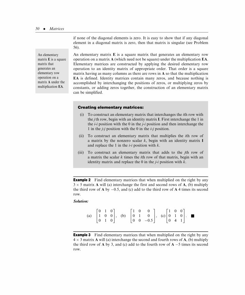
if none of the diagonal elements is zero. It is easy to show that if any diagonal
element in a diagonal matrix is zero, then that matrix is singular (see Problem
56).
An elementary matrix E is a square matrix that generates an elementary row
operation on a matrix A (which need not be square) under the multiplication EA.
Elementary matrices are constructed by applying the desired elementary row
operation to an identity matrix of appropriate order. That order is a square
matrix having as many columns as there are rows in A so that the multiplication
EA is defined. Identity matrices contain many zeros, and because nothing is
accomplished by interchanging the positions of zeros, or multiplying zeros by
constants, or adding zeros together, the construction of an elementary matrix
can be simplified.
Example 2 Find elementary matrices that when multiplied on the right by any
3� 5 matrix A will (a) interchange the first and second rows of A, (b) multiply
the third row of A by �0:5, and (c) add to the third row of A 4 times its second
row.
Solution:
(a)
0 1 0
1 0 0
0 1 0
24
35, (b)
1 0 0
0 1 0
0 0 �0:5
24
35, (c)
1 0 0
0 1 0
0 4 1
24
35: &
Example 3 Find elementary matrices that when multiplied on the right by any
4� 3 matrix A will (a) interchange the second and fourth rows of A, (b) multiply
the third row of A by 3, and (c) add to the fourth row of A �5 times its second
row.
Creating elementary matrices:
(i) To construct an elementary matrix that interchanges the ith row with
the j th row, begin with an identity matrix I. First interchange the 1 in
the i-i position with the 0 in the j-i position and then interchange the
1 in the j-j position with the 0 in the i-j position.
(ii) To construct an elementary matrix that multiplies the ith row of
a matrix by the nonzero scalar k, begin with an identity matrix I
and replace the 1 in the i-i position with k.
(iii) To construct an elementary matrix that adds to the jth row of
a matrix the scalar k times the ith row of that matrix, begin with an
identity matrix and replace the 0 in the j-i position with k.
An elementary
matrix E is a square
matrix that
generates an
elementary row
operation on a
matrix A under the
multiplication EA.
50 . Matrices

Solution:
(a)
1 0 0 0
0 0 0 1
0 0 1 0
0 1 0 0
2664
3775, (b)
1 0 0 0
0 1 0 0
0 0 3 0
0 0 0 1
2664
3775, (c)
1 0 0 0
0 1 0 0
0 0 1 0
0 �5 0 1
2664
3775:
" Theorem 1. (a) The inverse of an elementary matrix that inter-
changes two rows is the elementary matrix itself.
(b) The inverse of an elementary matrix that multiplies
one row by a nonzero scalar k is a matrix obtained
by replacing the scalar k in the elementary matrix
by 1/k.
(c) The inverse of an elementary matrix that adds to one
row a constant k times another row is a matrix
obtained by replacing the scalar k in the elementary
matrix by �k.
"
Proof: (a) Let E be an elementary matrix that has the effect interchanging the
i th and j th rows of a matrix. E comes from interchanging the i th and j th rows of
the identity matrix having the same order as E. Then EE ¼ I, because interchang-
ing the positions of the ith row of an identity matrix with jth row twice in
succession does not alter the original matrix. With EE ¼ I, it follows that
E�1 ¼ E.
(b) Let E be an elementary matrix that has the effect of multiplying the ith row of
a matrix by a nonzero scalar k, and let F be an elementary matrix that has the
effect of multiplying the ith row of a matrix by a nonzero scalar 1/k. E comes
from multiplying the ith of the identity matrix having the same order as E by k.
Then FE ¼ I, because multiplying the ith row of an identity matrix first by k and
then by 1/k does not alter the original matrix. With FE ¼ I, it follows that
F ¼ E�1.
(c) The proof is similar to the part (b) and is left as an exercise for the reader (see
Problem 63). &
Example 4 The inverses of the elementary matrices found in Example 2 are,
respectively,
(a)
0 1 0
1 0 0
0 1 0
24
35, (b)
1 0 0
0 1 0
0 0 �2
24
35, (c)
1 0 0
0 1 0
0 �4 1
24
35:
1.5 The Inverse . 51

The inverses of the elementary matrices found in Example 3 are, respectively,
(a)
1 0 0 0
0 0 0 1
0 0 1 0
0 1 0 0
2664
3775, (b)
1 0 0 0
0 1 0 0
0 0 1=3 0
0 0 0 1
2664
3775, (c)
1 0 0 0
0 1 0 0
0 0 1 0
0 5 0 1
2664
3775: &
Elementary row operations are the backbone of a popular method for calculat-
ing inverses. We shall show in Section 2.6 that a square matrix is invertible if and
only if it can be transformed into a row-reduced matrix having all ones on the
main diagonal. If such a transformation is possible, then the original matrix can
be reduced still further, all the way to an identity matrix. This is done by
applying elementary row operation R3—adding to one row of a matrix a scalar
times another row of the same matrix—to each column, beginning with the last
column and moving sequentially towards the first column, placing zeros in all
positions above the diagonal elements.
Example 5 Use elementary row operations to transform the row-reduced matrix
A ¼1 2 1
0 1 3
0 0 1
24
35
to the identity matrix.
Solution:
1 2 1
0 1 3
0 0 1
24
35! 1 2 1
0 1 0
0 0 1
24
35 by adding to
the second row
�3 times the third row
!1 2 0
0 1 0
0 0 1
24
35 by adding to
the first row
�1 times the third row
!1 0 0
0 1 0
0 0 1
24
35 by adding to the
first row �2 times &
the second row
Thus, a square A has an inverse if and only if A can be transformed into an
identity matrix with elementary row operations. Because each elementary row
operation can be represented by an elementary matrix, we conclude that a matrix
A has an inverse if and only if there exists a sequence of elementary matrices
E1, E2, . . . , Ek such that
EkEk�1 . . . E2E1A ¼ I
52 . Matrices

Denoting the product of these elementary matrices by B, we have BA ¼ I, which
implies that B ¼ A�1. To calculate the inverse of a matrix A, we need only record
the product of the elementary row operations used to transform A to I. This is
accomplished by applying the same elementary row operations to both A and
I simultaneously.
Example 6 Find the inverse of A ¼ 1 2
3 4
� �.
Solution:
1 2
3 4
1 0
0 1
����� �
!1 2
0 �2
1 0
�3 1
����� � by adding to
the second row �3
times the first row
!0 2
0 1
1 0
3=2 �1=2
�����
by multiplying the
second row by �1=2
�
A has been transformed into row-reduced form with a main diagonal of only
ones; A has an inverse. Continuing with the transformation process, we get
! 1 0
0 1
�2 1
3=2 �1=2
����� � by adding to the
first row �2 times
the second row
Thus,
A�1 ¼ �2 1
3=2 �1=2
� �&
Calculating inverses:
Step 1. Create an augmented matrix [A j I], where A is the n� n matrix to
be inverted and I is the n� n identity matrix.
Step 2. Use elementary row operations on [A j I] to transform the left
partition A to row-reduced form, applying each operation to the
full augmented matrix.
Step 3. If the left partition of the row-reduced matrix has zero elements
on its main diagonal, stop: A does not have inverse. Otherwise,
continue.
Step 4. Use elementary row operations on the row-reduced augmented
matrix to transform the left partition to the n� n identity matrix,
applying each operation to the full augmented matrix.
Step 5. The right partition of the final augmented matrix is the inverse
of A.
1.5 The Inverse . 53

Example 7 Find the inverse of A ¼5 8 1
0 2 1
4 3 �1
24
35
Solution:
5 8 1
0 2 1
4 3 �1
1 0 0
0 1 0
0 0 1
�������264
375
!1 1:6 0:20 2 1
4 3 �1
0:2 0 0
0 1 0
0 0 1
������24
35 by multiplying the
first row by 0:2
!1 1:6 0:20 2 1
0 �3:4 �1:8
0:2 0 0
0 1 0
�0:8 0 1
������24
35 by adding to the
third row �4 times
the first row
!1 1:6 0:20 1 0:50 �3:4 �1:8
0:2 0 0
0 0:5 0
�0:8 0 1
������24
35 by multiplying the
second row by 1=2
!1 1:6 0:20 1 0:50 0 �0:1
0:2 0 0
0 0:5 0
�0:8 1:7 1
������24
35 by adding to the
third row 3:4 times
the second row
!1 1:6 0:20 1 0:50 0 1
0:2 0 0
0 0:5 0
8 �17 �10
������24
35 by multiplying the
third row by �10
A has been transformed into row-reduced form with a main diagonal of only
ones; A has an inverse. Continuing with the transformation process, we get
!1 1:6 0:20 1 0
0 0 1
0:2 0 0
�4 9 5
8 �17 �10
������24
35 by adding to the
second row �0:5times the third row
!1 1:6 0
0 1 0
0 0 1
�1:4 3:4 2
�4 9 5
8 �17 �10
������24
35 by adding to the
first row �0:2times the third row
!1 0 0
0 1 0
0 0 1
5 �11 6
�4 9 5
8 �17 �10
������24
35 by adding to the
first row �1:6 timesthe second row
54 . Matrices

Thus,
A�1 ¼5 �11 �6
�4 9 5
8 �17 �10
24
35 &
Example 8 Find the inverse of A ¼0 1 1
1 1 1
1 1 3
24
35:
Solution:
0 1 1
1 1 1
1 1 3
1 0 0
0 1 0
0 0 1
�������264
375
!1 1 1
0 1 1
1 1 3
0 1 0
1 0 0
0 0 1
������24
35 by interchanging the
first and second rows
!1 1 1
0 1 1
0 0 2
0 1 0
1 0 0
0 �1 1
������24
35 by adding to the
third row �1 timesthe first row
!1 1 1
0 1 1
0 0 1
0 1 0
1 0 0
0 �1=2 1=2
������24
35 by multiplying the
third row by 1=2
!1 1 1
0 1 0
0 0 1
0 1 0
1 1=2 �1=20 �1=2 1=2
������24
35 by adding to the
second row �1times the third row
!1 1 0
0 1 0
0 0 1
0 3=2 �1=21 1=2 �1=20 �1=2 1=2
������24
35 by adding to the
first row �1 timesthe third row
!1 0 0
0 1 0
0 0 1
�1 1 0
1 1=2 �1=20 �1=2 1=2
������24
35 by adding to the
first row �1 times thesecond row
Thus,
A�1 ¼�1 1 0
1 1=2 �1=20 �1=2 1=2
24
35 &
1.5 The Inverse . 55

Example 9 Find the inverse of A ¼ 1 2
2 4
� �:
Solution:
1 2
2 4
1 0
0 1
����� �
! 1 2
0 0
1 0
�2 1
����� � by adding to the
second row �2times the first row
A has been transformed into row-reduced form. Because the main diagonal
contains a zero entry, A does not have an inverse; A is singular. &
" Theorem 2. The inverse of a matrix is unique.
"
Proof: If B and C are both inverses of the matrix A, then
AB ¼ I, BA ¼ I, AC ¼ I, and CA ¼ I:
It now follows that
C ¼ CI ¼ C(AB) ¼ (CA)B ¼ IB ¼ B:
Thus, if B and C are both inverses of A, they must be equal; hence, the inverse
is unique. &
Using Theorem 2, we can prove some useful properties of inverses.
" Theorem 3. If A and B are n� n nonsingular matrices, then
(a) (A�1)�1 ¼ A,
(b) (AB)�1 ¼ B�1A�1,
(c) (AT)�1 ¼ (A�1)
T,
(d) (lA)�1 ¼ (1=l)A�1, if l is a nonzero scalar.
"
Proof: We prove parts (b) and (c) and leave parts (a) and (d) as exercises (see
Problems 59 and 60). To prove (b), we note that
(B�1A�1) (AB) ¼ B�1(A�1A) B ¼ B�1 IB ¼ B�1 B ¼ I:
Thus, B�1A�1 is an inverse of AB. Because the inverse is unique, it follows that
(AB)�1 ¼ B�1A�1.
56 . Matrices

To prove (c), we note that
(AT) (A�1)T ¼ (A�1A)
T ¼ IT ¼ I:
Thus, (A�1)T is an inverse of AT. Because the inverse is unique, it follows that
(AT)�1 ¼ (A�1)T. &
The process of finding an inverse is known as inversion, and, interestingly, some
matrix forms are preserved under this process.
" Theorem 4. (a) The inverse of a nonsingular symmetric matrix is
symmetric.
(b) The inverse of a nonsingular upper or lower trian-
gular matrix is again an upper or lower triangular
matrix, respectively.
"
Proof: If A is symmetric, then AT ¼ A. Combining this observation with part
(c) of Theorem 2, we find that
(A�1)T ¼ (AT)
�1 ¼ (A)�1
so A�1 also equals its transpose and is symmetric. This proves part (a). Part (b) is
immediate from Theorem 2 and the constructive procedure used for calculating
inverses. The details are left as an exercise (see Problem 62).
A system of simultaneously linear equations has the matrix form
Ax ¼ b (1:14 repeated)
If the coefficient matrix A is invertible, we can premultiply both sides of equation
(1.14) by A�1 to obtain
A�1(Ax) ¼ A�1b
(A�1A)x ¼ A�1b
Ix ¼ A�1b
or
x ¼ A�1b & (1:25)
This is precisely the form we sought in Section 1.2. With this formula, we can
solve for all the variables in a system of linear equations at the same time.
The matrix equation
Ax ¼ b has
x ¼ A�1b as its
solution if the
coefficient matrix
A is invertible.
1.5 The Inverse . 57

Example 10 The system of equations
xþ 2y ¼ 150
3xþ 4y ¼ 250
can be written as Ax ¼ b with
A ¼ 1 2
3 4
� �, x ¼ x
y
� �, and b ¼ 150
250
� �
Using the results of Example 6, we have that the coefficient matrix A is
invertible and
x
y
� �¼ x ¼ A�1b ¼ �2 1
3=2 �1=2
� �150
250
� �¼ �50
100
� �:
Hence, x ¼ �50 and y ¼ 100. &
Example 11 The system of equations
5xþ 8yþ z ¼ 2
2yþ z ¼ �1
4xþ 3y� z ¼ 3
can be written as Ax ¼ b with
A ¼5 8 1
0 2 1
4 3 �1
24
35, x ¼
x
y
z
2435, and b ¼
2
�1
3
24
35:
Using the results of Example 7, we have that the coefficient matrix A is
invertible and
x
y
� �¼ x ¼ A�1b ¼
5 �11 �6
�4 9 5
8 �17 �10
24
35 2
�1
3
24
35 ¼ 3
�2
3
24
35
Hence, x ¼ 3, y ¼ �2, and z ¼ 3: &
58 . Matrices

Not only does the invertibility of the coefficient matrix A provide us with
a solution to the system Ax ¼ b, it also provides us with a means to show that
this solution is the only solution to the system.
" Theorem 5. If A is invertible, then the system of simultaneous
linear equations defined by Ax ¼ b has a unique (one and only one)
solution.
"
Proof: Define w ¼ A�1b. Then
Aw ¼ AA�1b ¼ Ib ¼ b (1:26)
and w is one solution to the system Ax ¼ b. Let y be another solution to this
system. Then necessarily
Ay ¼ b (1:27)
Equations (1.26) and (1.27) imply that
Aw ¼ Ay
Premultiplying both sides of this last equation by A�1, we find
A�1(Aw) ¼ A�1(Ay)
(A�1A)w ¼ (A�1A)y
Iw ¼ Iy
or
w ¼ y
Thus, if y is a solution of Ax ¼ b, then it must equal w. Therefore, w ¼ A�1b is
the only solution to this system. &
If A is singular, so that A�1 does not exist, then equation (1.25) is not valid and
other methods, such as Gaussian elimination, must be used to solve the given
system of simultaneous equations.
1.5 The Inverse . 59

Problems 1.5
(1) Determine if any of the following matrices are inverses for A ¼ 1 3
2 9
� �:
(a)1 1=3
1=2 1=9
� �, (b)
�1 �3
�2 �9
� �,
(c)3 �1
�2=3 1=3
� �, (d)
9 �3
�2 1
� �.
(2) Determine if any of the following matrices are inverses for A ¼ 1 1
1 1
� �:
(a)1 1
1 1
� �, (b)
�1 1
1 �1
� �,
(c)1 1
�1 �1
� �, (d)
2 �1
�1 2
� �.
In Problems 3 through 12, find elementary matrices that when multiplied on the right by
the given matrix A will generate the specified result.
(3) Interchange the order of the first and second rows of a 2� 2 matrix A.
(4) Multiply the first row of a 2� 2 matrix A by 3.
(5) Multiply the second row of a 2� 2 matrix A by �5.
(6) Multiply the second row of a 3� 3 matrix A by �5.
(7) Add to the second row of a 2� 2 matrix A three times its first row.
(8) Add to the first row of a 2� 2 matrix A three times its second row.
(9) Add to the second row of a 3� 3 matrix A three times its third row.
(10) Add to the third row of a 3� 4 matrix A five times its first row.
(11) Interchange the order of the second and fourth rows of a 6� 6 matrix A.
(12) Multiply the second row of a 2� 5 matrix A by 7.
In Problems 13 through 22, find the inverses of the given elementary matrices.
(13)2 0
0 1
� �(14)
1 2
0 1
� �(15)
1 0
�3 1
� �
(16)1 0
1 1
� �(17)
1 0 0
0 2 0
0 0 1
24
35 (18)
0 1 0
1 0 0
0 0 1
24
35
(19)
1 0 3
0 1 0
0 0 1
24
35 (20)
1 0 0
0 1 �2
0 0 1
24
35 (21)
1 0 0 0
0 1 0 0
0 0 0 1
0 0 1 0
2664
3775
(22)
1 0 0 0
0 1 0 0
�3 0 1 0
0 0 0 1
2664
3775A�1 ¼ A
60 . Matrices

In Problems 23 through 39, find the inverses of the given matrices, if they exist.
(23)1 1
3 4
� �(24)
2 1
1 2
� �(25)
4 4
4 4
� �
(26)
1 1 0
1 0 1
0 1 1
24
35 (27)
0 0 1
1 0 0
0 1 0
24
35 (28)
2 0 �1
0 1 2
3 1 1
24
35
(29)
1 2 3
4 5 6
7 8 9
24
35 (30)
2 0 0
5 1 0
4 1 1
24
35 (31)
2 1 5
0 3 �1
0 0 2
24
35
(32)
3 2 1
4 0 1
3 9 2
24
35 (33)
1 2 �1
2 0 1
�1 1 3
24
35
(34)
1 2 1
3 �2 �4
2 3 �1
24
35 (35)
2 4 3
3 �4 �4
5 0 �1
24
35
(36)
5 0 �1
2 �1 2
2 3 �1
24
35 (37)
3 1 1
1 3 �1
2 3 �1
24
35
(38)
1 1 1 2
0 1 �1 1
0 0 2 3
0 0 0 �2
2664
3775 (39)
1 0 0 0
2 �1 0 0
4 6 2 0
3 2 4 �1
2664
3775
(40) Show directly that the inverse of A ¼ a b
c d
� �, when ad � bc 6¼ 0 is
A�1 ¼ 1
ad � bc
d �b
�c a
� �
(41) Use the result of Problem (40) to calculate the inverses of
(a)1 1
3 4
� �and (b)
1 1=2%1=2 1=3
� �
In Problems 42 through 51, use matrix inversion, if possible, to solve the given systems of
equations:
(42) xþ 2y ¼ �3 (43) aþ 2b ¼ 5
3xþ y ¼ 1 �3aþ b ¼ 13
(44) 4xþ 2y ¼ 6 (45) 4l � p ¼ 1
2x� 3y ¼ 1 5l � 2p ¼ �1
(46) 2xþ 3y ¼ 8 (47) xþ 2y� z ¼ �1
6xþ 9y ¼ 24 2xþ 3yþ 2z ¼ 5
y� z ¼ 2
1.5 The Inverse . 61
(48) 2xþ 3y� z ¼ 4 (49) 60l þ 30mþ 20n ¼ 0
�x� 2yþ z ¼ �2 30l þ 20mþ 15n ¼ �10
3x� y ¼ 2 20l þ 15mþ 12n ¼ �10
(50) 2rþ 3s� 4t ¼ 12 (51) xþ 2y� 2z ¼ �1
3r� 2s ¼ �1 2xþ yþ z ¼ 5
8r� s� 4t ¼ 10 �xþ y� z ¼ �2
(52) Solve each of the following systems using the same inverse:
(a) 3xþ 5y ¼ 10 (b) 3xþ 5y ¼ �8
2xþ 3y ¼ 20 2xþ 3y ¼ 22
(c) 3xþ 5y ¼ 0:2 (d) 3xþ 5y ¼ 0
2xþ 3y ¼ 0:5 2xþ 3y ¼ 5
(53) Solve each of the following systems using the same inverse:
(a) 2xþ 4y ¼ 2 (b) 2xþ 4y ¼ 3
3xþ 2yþ z ¼ 8 3xþ 2yþ z ¼ 8
5x� 3yþ 7z ¼ 15 5x� 3yþ 7z ¼ 15
(c) 2xþ 4y ¼ 2 (d) 2xþ 4y ¼ 1
3xþ 2yþ z ¼ 9 3xþ 2yþ z ¼ 7
5x� 3yþ 7z ¼ 15 5x� 3yþ 7z ¼ 14
(54) If A is nonsingular matrix, we may define A�n ¼ (A�1)n, for any positive integer n.
Use this definition to find A�2 and A�3 for the following matrices:
(a)1 1
2 3
� �, (b)
2 5
1 2
� �, (c)
1 1
3 4
� �,
(d)
1 1 1
0 1 1
0 0 1
24
35, (e)
1 2 �1
0 1 �1
0 0 1
24
35:
(55) Prove that a square zero matrix does not have an inverse.
(56) Prove that if a diagonal matrix has at least one zero on its main diagonal, then that
matrix does not have an inverse.
(57) Prove that if A2 ¼ I, the A�1 ¼ A.
(58) If A is symmetric, prove the identity (BA�1)T(A�1BT)
�1 ¼ I.
(59) Prove that if A is invertible, then (A�1)�1 ¼ A.
(60) Prove that if A is invertible and if l is a nonzero scalar, then (lA)�1 ¼ (1=l)A�1.
(61) Prove that if A, B, and C are n� n nonsingular matrices, then (ABC)�1 ¼C�1B�1A�1.
(62) Prove that the inverse of a nonsingular upper (lower) triangular matrix is itself
upper (lower) triangular.
(63) Prove part (c) of Theorem 1.
62 . Matrices

(64) Show that if A can be partitioned into the block diagonal form
A ¼
A1
A2 0A3
. ..
0 Ak
2666666664
3777777775
with A1, A2, . . . , An all invertible, then
A�1 ¼
A�11
A�12 0
A�13
. ..
0 A�1k
26666666664
37777777775
1.6 LU DECOMPOSITION
Matrix inversion of elementary matrices is at the core of still another popular
method, known as LU decomposition, for solving simultaneous equations in
the matrix form Ax ¼ b. The method rests on factoring a nonsingular coefficient
matrix A into the product of a lower triangular matrix L with an upper triangular
matrix U. Generally, there are many such factorizations. If L is required to have all
diagonal elements equal to 1, then the decomposition, when it exists, is unique and
we may write
A ¼ LU (1:28)
with
L ¼
1 0 0 . . . 0
l21 1 0 . . . 0
l31 l32 1 . . . 0
..
. ... ..
. . .. ..
.
ln1 ln2 ln3 . . . 1
2666664
3777775
U ¼
u11 u12 u13 . . . u1n
0 u22 u23 . . . u2n
0 0 u23 . . . u3n
..
. ... ..
. . .. ..
.
0 0 0 . . . unn
2666664
3777775
1.6 LU Decomposition . 63

To decompose A into form (1.28), we first transform A to upper triangular form
using just the third elementary row operation R3. This is similar to transforming
a matrix to row-reduced form, except we no longer use the first two elementary
row operations. We do not interchange rows, and we do not multiply rows by
nonzero constants. Consequently, we no longer require that the first nonzero
element of each nonzero row be 1, and if any of the pivots are 0—which would
indicate a row interchange in the transformation to row-reduced form—then the
decomposition scheme we seek cannot be done.
Example 1 Use the third elementary row operation to transform the matrix
A ¼2 �1 3
4 2 1
�6 �1 2
24
35
into upper triangular form.
Solution:
A ¼2 �1 3
4 2 1
�6 �1 2
264
375! 2 �1 3
0 4 �5
�6 �1 2
264
375 by adding to the
second row � 2 timesthe first row
!2 �1 3
0 4 �5
0 �4 11
24
35 by adding to the
third row 3 timesthe first row
!2 �1 3
0 4 �5
0 0 6
24
35 by adding to the
third row 1 timesthe second row &
If a square matrix A can be reduced to upper triangular form U by a sequence
of elementary row operations of the third type, then there exists a sequence of
elementary matrices E21, E31, E41, . . . , En, n�1 such that
En, n�1 . . . E41E31E21
� �A ¼ U (1:29)
where E21 denotes the elementary matrix that places a 0 in the 2-1 position, E31
denotes the elementary matrix that places a 0 in the 3-1 position, E41 denotes the
elementary matrix that places a 0 in the 4-1 position, and so on. Since elementary
matrices have inverses, we can write (1.29) as
64 . Matrices
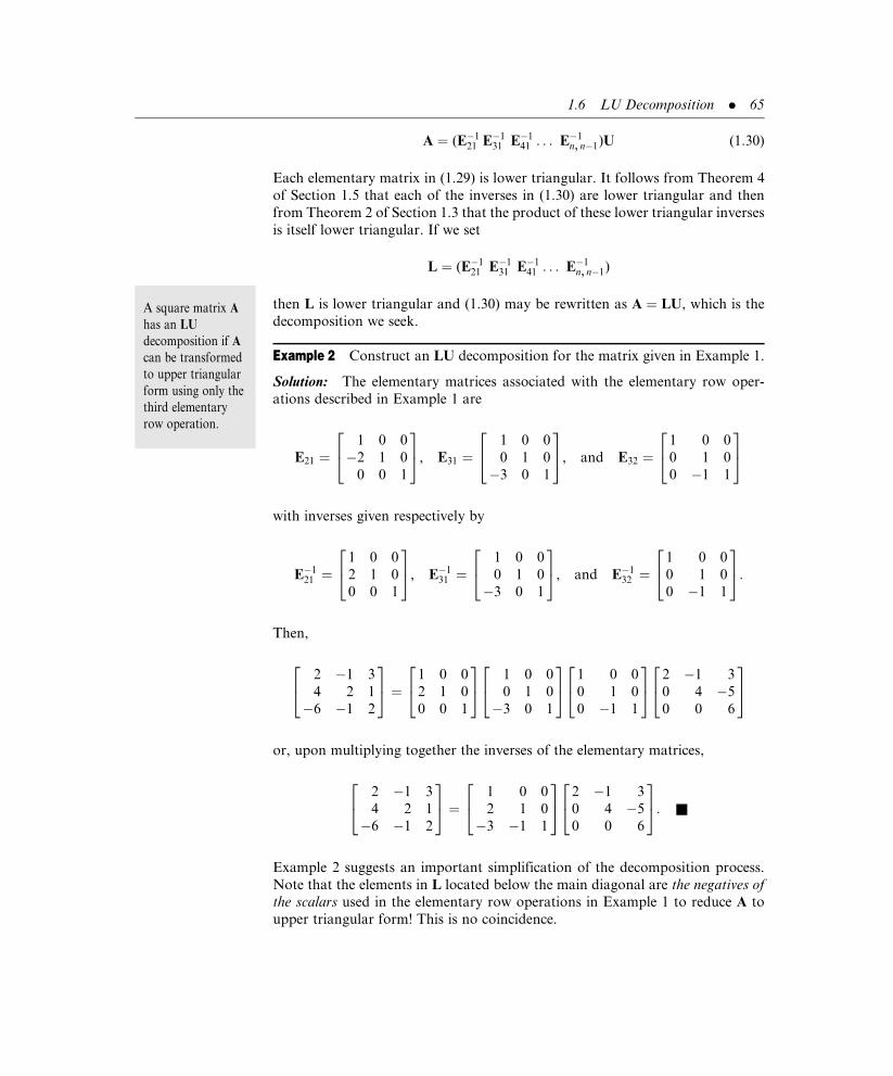
A ¼ (E�121 E�1
31 E�141 . . . E�1
n, n�1)U (1:30)
Each elementary matrix in (1.29) is lower triangular. It follows from Theorem 4
of Section 1.5 that each of the inverses in (1.30) are lower triangular and then
from Theorem 2 of Section 1.3 that the product of these lower triangular inverses
is itself lower triangular. If we set
L ¼ (E�121 E�1
31 E�141 . . . E�1
n, n�1)
then L is lower triangular and (1.30) may be rewritten as A ¼ LU, which is the
decomposition we seek.
Example 2 Construct an LU decomposition for the matrix given in Example 1.
Solution: The elementary matrices associated with the elementary row oper-
ations described in Example 1 are
E21 ¼1 0 0
�2 1 0
0 0 1
24
35, E31 ¼
1 0 0
0 1 0
�3 0 1
24
35, and E32 ¼
1 0 0
0 1 0
0 �1 1
24
35
with inverses given respectively by
E�121 ¼
1 0 0
2 1 0
0 0 1
24
35, E�1
31 ¼1 0 0
0 1 0
�3 0 1
24
35, and E�1
32 ¼1 0 0
0 1 0
0 �1 1
24
35:
Then,
2 �1 3
4 2 1
�6 �1 2
24
35 ¼ 1 0 0
2 1 0
0 0 1
24
35 1 0 0
0 1 0
�3 0 1
24
35 1 0 0
0 1 0
0 �1 1
24
35 2 �1 3
0 4 �5
0 0 6
24
35
or, upon multiplying together the inverses of the elementary matrices,
2 �1 3
4 2 1
�6 �1 2
24
35 ¼ 1 0 0
2 1 0
�3 �1 1
24
35 2 �1 3
0 4 �5
0 0 6
24
35: &
Example 2 suggests an important simplification of the decomposition process.
Note that the elements in L located below the main diagonal are the negatives of
the scalars used in the elementary row operations in Example 1 to reduce A to
upper triangular form! This is no coincidence.
A square matrix A
has an LU
decomposition if A
can be transformed
to upper triangular
form using only the
third elementary
row operation.
1.6 LU Decomposition . 65

" Observation 1. If, in transforming a square matrix A to upper triangular
form, a zero is placed in the i-j position by adding to row i a scalar k times
row j, then the i-j element of L in the LU decomposition of A is�k: 3
We summarize the decomposition process as follows: Use only the third ele-
mentary row operation to transform a square matrix A to upper triangular form.
If this is not possible, because of a zero pivot, then stop. Otherwise, the LU
decomposition is found by defining the resulting upper triangular matrix as U
and constructing the lower triangular matrix L according to Observation 1.
Example 3 Construct an LU decomposition for the matrix
A ¼
2 1 2 3
6 2 4 8
1 �1 0 4
0 1 �3 �4
2664
3775
Solution: Transforming A to upper triangular form, we get
2 1 2 3
6 2 4 8
1 �1 0 4
0 1 �3 �4
26664
37775!
2 1 2 3
0 �1 �2 �1
1 �1 0 4
0 1 �3 �4
26664
37775
by adding to the
second row � 3 times
the first row
!
2 1 2 3
0 �1 �2 �1
0 � 32�1 5
2
0 1 �3 �4
26664
37775
by adding to the
third row � 12
times
the first row
!
2 1 2 3
0 �1 �2 �1
0 0 2 4
0 1 �3 �4
2664
3775 by adding to the
third row� 32
timesthe second row
!
2 1 2 3
0 �1 �2 �1
0 0 2 4
0 0 �5 �5
2664
3775
by adding to the
fourth row 1 times
the second row
!
2 1 2 3
0 �1 �2 �1
0 0 2 4
0 0 0 5
2664
3775 by adding to the
fourth row 52
timesthe third row
66 . Matrices

We now have an upper triangular matrix U. To get the lower triangular matrix L
in the decomposition, we note that we used the scalar �3 to place a 0 in the 2-1
position, so its negative �(� 3) ¼ 3 goes into the 2-1 position of L. We used the
scalar �12
to place a 0 in the 3-1 position in the second step of the preceding
triangularization process, so its negative, 12, becomes the 3-1 element in L; we
used the scalar 52
to place a 0 in the 4-3 position during the last step of the
triangularization process, so its negative, � 52, becomes the 4-3 element in L.
Continuing in this manner, we generate the decomposition
2 1 2 3
6 2 4 8
1 �1 0 4
0 1 �3 �4
2664
3775 ¼
1 0 0 0
3 1 0 012
32
1 0
0 �1 � 52
1
2664
3775
2 1 2 3
0 �1 �2 �1
0 0 2 4
0 0 0 5
2664
3775 &
LU decompositions, when they exist, are used to solve systems of simultaneous
linear equations. If a square matrix A can be factored into A ¼ LU, then the
system of equations Ax ¼ b can be written as L(Ux) ¼ b. To find x, we first solve
the system
Ly ¼ b (1:31)
for y, and then once y is determined, we solve the system
Ux ¼ y (1:32)
for x. Both systems (1.31) and (1.32) are easy to solve, the first by forward
substitution and the second by backward substitution.
Example 4 Solve the system of equations:
2x� yþ 3z ¼ 9
4xþ 2yþ z ¼ 9
�6x� yþ 2z ¼ 12
Solution: This system has the matrix form
2 �1 3
4 2 1
�6 �1 2
264
375
x
y
z
264375 ¼
9
9
12
264
375
If A ¼ LU for a
square matrix A,
then the equation
Ax ¼ b is solved by
first solving the
equation Ly ¼ b for
y and then solving
the equation Ux ¼ y
for x.
1.6 LU Decomposition . 67

The LU decomposition for the coefficient matrix A is given in Example 2. If
we define the components of y by a, b, and g, respectively, the matrix system
Ly ¼ b is
1 0 0
2 1 0
�3 �1 1
264
375
a
b
g
264
375 ¼
9
9
12
264
375
which is equivalent to the system of equations
a ¼ 9
2aþ b ¼ 9
�3a� bþ g ¼ 12
Solving this system from top to bottom, we get a ¼ 9, b ¼ �9, and g ¼ 30.
Consequently, the matrix system Ux ¼ y is
2 �1 3
0 4 �5
0 0 6
24
35 x
y
z
2435 ¼ 9
�9
30
24
35
which is equivalent to the system of equations
2x� yþ 3z ¼ 9
4y� 5z ¼ �9
6z ¼ 30
Solving this system from bottom to top, we obtain the final solution
x ¼ �1, y ¼ 4, and z ¼ 5. &
Example 5 Solve the system
2aþ bþ 2cþ 3d ¼ 5
6aþ 2bþ 4cþ 8d ¼ 8
a� bþ 4d ¼ �4
b� 3c� 4d ¼ �3
68 . Matrices

Solution: The matrix representation for this system has as its coefficient matrix
the matrix A of Example 3. Define
y ¼ [a, b, g, d]T
Then, using the decomposition determined in Example 3, we can write the matrix
system Ly ¼ b as the system of equations
a ¼ 5
3aþ b ¼ 8
1
2aþ 3
2bþ g ¼ �4
�b� 5
2g þ d ¼ �3
which has as its solution a ¼ 5, b ¼ �7, g ¼ 4, and � ¼ 0. Thus, the matrix
system Ux ¼ y is equivalent to the system of equations
2aþ bþ 2cþ 3d ¼ 5
�b� 2c� d ¼ �7
2cþ 4d ¼ 4
5d ¼ 0
Solving this set from bottom to top, we calculate the final solution as
a ¼ �1, b ¼ 3, c ¼ 2, and d ¼ 0. &
Problems 1.6
In Problems 1 through 14, A and b are given. Construct an LU decomposition for the
matrix A and then use it to solve the system Ax ¼ b for x.
(1) A ¼ 1 1
3 4
� �, b ¼ 1
�6
� �. (2) A ¼ 2 1
1 2
� �, b ¼ 11
�2
� �.
(3) A ¼ 8 3
5 2
� �, b ¼ 625
550
� �. (4) A ¼
1 1 0
1 0 1
0 1 1
24
35, b ¼
4
1
�1
24
35.
(5) A ¼�1 2 0
1 �3 1
2 �2 3
24
35, b ¼
�1
�2
3
24
35.
(6) A ¼2 1 3
4 1 0
�2 �1 �2
24
35, b ¼
10
�40
0
24
35.
1.6 LU Decomposition . 69

(7) A ¼3 2 1
4 0 1
3 9 2
24
35, b ¼
50
80
20
24
35.
(8) A ¼1 2 �1
2 0 1
�1 1 3
24
35, b ¼
80
159
�75
24
35.
(9) A ¼1 2 �1
0 2 1
0 0 1
24
35, b ¼
8
�1
5
24
35.
(10) A ¼1 0 0
3 2 0
1 1 2
24
35, b ¼
2
4
2
2435.
(11) A ¼
1 0 1 1
1 1 0 1
1 1 1 0
0 1 1 1
2664
3775, b ¼
4
�3
�2
�2
2664
3775.
(12) A ¼
2 1 �1 3
1 4 2 1
0 0 �1 1
0 1 0 1
2664
3775, b ¼
1000
200
100
100
2664
3775.
(13) A ¼
1 2 1 1
1 1 2 1
1 1 1 2
0 1 1 1
2664
3775, b ¼
30
30
10
10
2664
3775.
(14) A ¼
2 0 2 0
2 2 0 6
�4 3 1 1
1 0 3 1
2664
3775, b ¼
�2
4
9
4
2664
3775.
(15) (a) Use LU decomposition to solve the system
�xþ 2y ¼ �9
2xþ 3y ¼ 4
(b) Use the decomposition to solve the preceding system when the right sides of
the equations are replaced by 1 and �1, respectively.
(16) (a) Use LU decomposition to solve the system
xþ 3y� z ¼� 1
2xþ 5yþ z ¼ 4
2xþ 7y� 4z ¼� 6
(b) Use the decomposition to solve the preceding system when the right side of
each equation is replaced by 10, 10, and 10, respectively.
70 . Matrices

(17) Solve the system Ax ¼ b for the following vectors b when A is given as in
Problem 4:
(a)
5
7
�4
24
35, (b)
2
2
0
2435, (c)
40
50
20
24
35, (d)
1
1
3
2435:
(18) Solve the system Ax ¼ b for the following vectors b when A is given as in
Problem 13:
(a)
�1
1
1
1
2664
3775, (b)
0
0
0
0
26643775, (c)
190
130
160
60
2664
3775, (d)
1
1
1
1
26643775.
(19) Show that LU decomposition cannot be used to solve the system
2yþ z ¼ �1
xþ yþ 3z ¼ 8
2x� y� z ¼ 1
but that the decomposition can be used if the first two equations are interchanged.
(20) Show that LU decomposition cannot be used to solve the system
xþ 2yþ z ¼ 2
2xþ 4y� z ¼ 7
xþ yþ 2z ¼ 2
but that the decomposition can be used if the first and third equations are inter-
changed.
(21) (a) Show that the LU decomposition procedure given in this section cannot be
applied to
A ¼ 0 2
0 9
� �
(b) Verify that A ¼ LU, when
L ¼ 1 0
1 1
� �and U ¼ 0 2
0 7
� �
(c) Verify that A ¼ LU, when
L ¼ 1 0
3 1
� �and U ¼ 0 2
0 3
� �
1.6 LU Decomposition . 71

(d) Why do you think the LU decomposition procedure fails for this A? What might
explain the fact that A has more than one LU decomposition?
1.7 PROPERTIES OF Rn
Points on the plane in an x-y coordinate system are identified by an ordered pair
of real numbers; points in space are located by an ordered triplet of real numbers.
These are just two examples of the more general concept of an ordered array of
n-real numbers known as an n-tuple. We write an n-tuple as a 1� n row matrix.
The elements in the row matrix are real numbers and the number of elements
(columns) n is the dimension of the row matrix. The set of all n-tuples is often
referred to as n-space and denoted by Rn. In particular, the ordered pair [ 1 2 ] is
a member of R2; it is a 2-tuple of dimension two. The ordered triplet
[ 10 20 30 ] is a member of R3; it is a 3-tuple of dimension three. The p-tuple
a ¼ [ a1 a2 a3 . . . ap ], where aj (j ¼ 1, 2, . . . , p) is a real number, is a
member of Rp, and has dimension p.
An ordered array of real numbers also can be written as a column matrix, and
often is. Here we work exclusively with row matrix representations, but only as
a matter of convenience. We could work equally well with column matrices.
Row matrices are special types of matrices, those matrices having only one row,
so the basic matrix operations defined in Section 1.1 remain valid for n-tuples
represented as row matrices. This means we know how to add and subtract
n-tuples of the same dimension and how to multiple a real number times an
n-tuple (scalar multiplication). If we restrict ourselves to R2 and R3, we can
describe these operations geometrically.
A two-dimensional row matrix v ¼ [ a b ] is identified with the point (a, b) on
x-y plane, measured a units along the horizontal x-axis from the origin and then
b units parallel to the vertical y-axis. If we draw a directed line segment, or
arrow, beginning at the origin and ending at the point (a, b), then this arrow, as
shown in Figure 1.10, is a geometrical representation of the row matrix [ a b ]. It
follows immediately from Pythagoras’s theorem that the length or magnitude of
v, denoted by kvk, is
vk k ¼ a b½ �k k ¼ffiffiffiffiffiffiffiffiffiffiffiffiffiffiffia2 þ b2
p
and from elementary trigonometry that the angle u satisfies the equation
tan u ¼ b
a
Rn is the set of
ordered arrays of n
real numbers. This
set is represented
either by the set of
all n-dimensional
row matrices or by
the set of all n-
dimensional column
matrices.
72 . Matrices

Example 1 Represent the row matrices v ¼ [ 2 4 ] and u ¼ [�1 1 ]
geometrically and then determine the magnitude of each and the angle each
makes with the horizontal x-axis.
Solution: The row matrices are graphed in Figure 1.11. For v, we have
vk k ¼ffiffiffiffiffiffiffiffiffiffiffiffiffiffiffiffiffiffiffiffiffi(2)2 þ (4)2
q� 4:47, tan u ¼ 4
2¼ 2, and u � 63:4�
For u, similar computations yield
uk k ¼ffiffiffiffiffiffiffiffiffiffiffiffiffiffiffiffiffiffiffiffiffiffiffiffiffiffiffi(� 1)2 þ (1)2
q� 1:14, tan u ¼ 1
�1¼ �1, and u ¼ 135� &
Figure 1.10
(a, b)
a
b
y
vector v
xθ
Figure 1.11
1
−1
−1−2 2 31
2
3
4
(−1, 1)
(2, 4)
vect
or v
vector u
y
x
1.7 Properties of Rn . 73

To geometrically construct the sum of two row matrices u and v in R2, graph u
and v on the same coordinate system, translate v so its initial point coincides with
the terminal point of u, being careful to preserve both the magnitude and direction
of v, and then draw an arrow from the origin to the terminal point of v after
translation. This arrow geometrically represents the sum uþ v. The process is
illustrated in Figure 1.12 for the row matrices u ¼ [�1 1 ] and v ¼ [ 2 4 ].
To construct the difference of two row matrices u� v geometrically, graph both
u and v normally and construct an arrow from the terminal point of v to the
terminal point of u. This arrow geometrically represents the difference u� v. The
process is depicted in Figure 1.13 for u ¼ [�1 1 ] and v ¼ [ 2 4 ].
Figure 1.12
5
4
3
3
2
2
1
1x
y
−2
−1
−1
u
vu
+ v
v tra
nsla
ted
Figure 1.13
u − v
1
−1
−1−2 2 31
2
3
4
y
x
v
u
To graph uþ v in
R2, graph u and v on
the same coordinate
system, translate v
so its initial point
coincides with the
terminal point of u,
and then draw an
arrow from the
origin to the
terminal point of v
after translation.
To graph u� v in
R2, graph u and v on
the same coordinate
system and then
draw an arrow from
the terminal point of
v to the terminal
point of u.
74 . Matrices

Translating an arrow (directed line segment) that represents a two-dimensional
row matrix from one location in the plane to another does not affect the
representation, providing both the magnitude and direction as defined by the
angle the arrow makes with the positive x-axis are preserved. Many physical
phenomena such as velocity and force are completely described by their magni-
tudes and directions. A wind velocity of 60 miles per hour in the northwest
direction is a complete description of that velocity, and it is independent of where
that wind occurs, be it Lawrence, Kansas, or Portland, Oregon. This independ-
ence is the rationale behind translating row matrices geometrically. Geometric-
ally, two-dimensional row matrices having the same magnitude and direction are
call equivalent, and they are regarded as being equal even though they may be
located at different positions in the plane. The four arrows drawn in Figure 1.14
are all geometrical representations of the same row matrix [ 1 �3 ].
To recapture a row matrix from the directed line segment that represents it, we
translate the directed line segment so that its tail lies on the origin and then read
the coordinates of its tip. Alternatively, we note that if a directed line segment w
does not originate at the origin, then it can be expressed as the difference between
a directed line segment u that begins at the origin and ends at the tip of w and
a directed line segment v that originates at the origin and ends at the tail of w as
Figure 1.14 y
x
Figure 1.15 y
x
w
v
u
1.7 Properties of Rn . 75

shown in Figure 1.15. Therefore, if the tip of w is at the point (x2, y2) and the tail
at the point (x1, y1), then u represents the row matrix [ x2 y2 ], v represents the
row matrix [ x1 y1 ], and w is the difference w ¼ u� v ¼ [ x2 � x1 y2 � y1 ].
Example 2 Determine the two-dimensional row matrix associated with the
directed line segments w and z shown in Figure 1.16.
Solution: The tip of the directed line segment w is at the point (40, 30) while its
tail lies on the point (10, � 20), so
w ¼ [ 40� 10 30� (� 20) ] ¼ [ 30 50 ]
The tip of the directed line segment z is at the point (� 10, 30) while its tail lies on
the point (� 50, 50), so
z ¼ [�10� (� 50) 30� 50 ] ¼ [ 40 �20 ] &
A scalar multiplication ku is defined geometrically in R2 to be a directed line
segment having length jkj times the length of u, in the same direction as u when
k is positive and in the opposite direction to u when k is negative. Effectively, ku
is an elongation of the directed line segment representing u when jkj is greater
than 1, or a contraction of u by a factor of jkj when jkj is less than 1, followed by
no rotation when k is positive or a rotation of 180 degrees when k is negative.
Example 3 Find �2u and 1⁄2 v geometrically for the row matrices u ¼ [�1 1 ]
and v ¼ [ 2 4 ].
Solution: To construct �2u, we double the length of u and then rotate the
resulting arrow by 180�. To construct 1⁄2 v, we halve the length of v and effect
no rotation. These constructions are illustrated in Figure 1.17. &
Figure 1.16
10 4030 5020−10−40 −30−50 −20
50
40
30
20
10
−10
−20
−30
−40
−50
y
x
z
w
The graph of ku in
R2 is a directed line
segment having
length jkj times the
length of u with the
same direction as u
when the scalar k is
positive and the
opposite direction
to u when k is
negative.
76 . Matrices

To graphically depict a three-dimensional row matrix, we first construct
a rectangular coordinate system defined by three mutually perpendicular lines,
representing the axes, that intersect at their respective origins. For convenience,
we denote these axes as the x-axis, the y-axis, and the z-axis, and their point of
intersection as the origin.
Rectangular coordinate systems are of two types: right-handed systems and left-
handed systems. An xyz system is right-handed if the thumb of the right hand
points in the direction of the positive z-axis when the fingers of the right hand are
curled naturally—in a way that does not break the finger bones—from the
positive x-axis towards the positive y-axis. In a left-handed system, the thumb
of the left hand points in the positive z-axis when the fingers of the left hand are
curled naturally from the positive x-axis towards the positive y-axis. Both types
of systems are illustrated in Figure 1.18. In this book, we shall only use right-
handed coordinate systems when graphing in space.
A three-dimensional row matrix v ¼ [ a b c ] is identified with the point (a, b,
c) in an xyz-coordinate system, measured a units along the x-axis from the
origin, then b units parallel to the y-axis, and then finally c units parallel to the
Figure 1.17
1
−1
−2
−1−2−3 2 31
2
3
4
y
x
12
u
−2u
v
Figure 1.18
Right-handed System Left-handed System
xx
yy
zz
1.7 Properties of Rn . 77

z-axis. An arrow or directed line segment having its tail at the origin and its tip at
the point (a, b, c) represents the row matrix v geometrically. The geometrical
representations of the row matrices u ¼ [ 2 4 6 ] and v ¼ [ 5 2 �3 ] are
illustrated in Figures 1.19 and 1.20, respectively.
All of the geometrical processes developed for the addition, subtraction, and
scalar multiplication of 2-tuples extend directly to 3-tuples. In particular,
to graph u� v, first graph both directed line segments normally and then
construct an arrow from the tip of v to the tip of u. Multiplication of a directed
line segment u by the scalar k is again an elongation of u by jkj when jkj is
greater than unity and a contraction of u by jkj when jkj is less than unity,
followed by no rotation when k is positive or a rotation of 180 degrees when
Figure 1.19
41
1
34
1
2
3
4
5
6
7
2
(2, 4, 0 )(2, 0, 0 )
(2, 4, 6 )
3 5 6y
z
u
x
Figure 1.20
(5, 2, −3)
1
x
y
z
v−3
−2
−1
2
12
34
6
3 4
(5, 0, 0)(5, 2, 0)
78 . Matrices

k is negative. If a directed line segment has its tip at the point (x2, y2, z2)
and its tail at the point (x1, y1, z1), then the row matrix associated with it is
[(x2 � x1) (y2 � y1) (z2 � z1)].
Although geometrical representations for Rn are limited to n � 3, the concept
of magnitude can be extended to all n-tuples. We define the magnitude of the
n-dimensional row matrix a ¼ [ a1 a2 a3 . . . an ] as
ak k ¼ffiffiffiffiffiffiffiffiffiffiffiffiffiffiffiffiffiffiffiffiffiffiffiffiffiffiffiffiffiffiffiffiffiffiffiffiffiffiffiffiffiffiffiffiffiffiffia2
1 þ a22 þ a2
3 þ . . .þ a2n
q(1:33)
Example 4 The magnitude of the 4-tuple a ¼ [ 1 2 3 4 ] is
ak k ¼ffiffiffiffiffiffiffiffiffiffiffiffiffiffiffiffiffiffiffiffiffiffiffiffiffiffiffiffiffiffiffiffiffiffiffiffiffiffiffiffiffiffiffiffiffiffiffiffi(1)2 þ (2)2 þ (3)2 þ (4)2
q¼
ffiffiffiffiffi30p
while the magnitude of the 5-tuple u ¼ [�4 �5 0 5 4 ] is
uk k ¼ffiffiffiffiffiffiffiffiffiffiffiffiffiffiffiffiffiffiffiffiffiffiffiffiffiffiffiffiffiffiffiffiffiffiffiffiffiffiffiffiffiffiffiffiffiffiffiffiffiffiffiffiffiffiffiffiffiffiffiffiffiffiffiffiffiffiffiffiffiffiffiffiffi(� 4)2 þ (� 5)2 þ (0)2 þ (5)2 þ (4)2
q¼
ffiffiffiffiffi82p
&
An n-tuple is normalized if it has a magnitude equal to one. Any n-tuple
(row matrix) is normalized by multiplying the n-tuple by the reciprocal of its
magnitude.
Example 5 As shown in Example 4, a ¼ [ 1 2 3 4 ] has magnitude
ak k ¼ffiffiffiffiffi30p
, so
1ffiffiffiffiffi30p 1 2 3 4½ � ¼ 1ffiffiffiffiffi
30p 2ffiffiffiffiffi
30p 3ffiffiffiffiffi
30p 4ffiffiffiffiffi
30p
� �
is normalized. Similarly, u ¼ [�4 �5 0 5 4 ] has magnitude uk k ¼ffiffiffiffiffi82p
, so
1ffiffiffiffiffi82p �4 �5 0 5 4½ � ¼ �4ffiffiffiffiffi
82p �5ffiffiffiffiffi
82p 0
5ffiffiffiffiffi82p 4ffiffiffiffiffi
82p
� �
is normalized. &
Two row matrices of the same dimension can be added and subtracted but they
cannot be multiplied. Multiplication of a 1� n matrix by another 1� n matrix is
undefined. Scalar multiplication of row matrices is defined but inversion is not
An n-tuple is
normalized if it has
a magnitude equal
to one.
1.7 Properties of Rn . 79

defined for row matrices of dimension greater than 1, because such row matrices
are not square. Thus, row matrices, and therefore n-tuples, do not possess all the
properties of real numbers. Listing the properties that n-tuples do share with real
numbers and then developing an algebra around those properties is the focus of
the next chapter.
In preparation for our work in Chapter 2, we list some of the important
properties shared by all n-tuples. If a, b, and c denote row matrices of the same
dimension n, then it follows from Theorem 1 of Section 1.1 that
aþ b ¼ bþ c (1:34)
and
aþ (bþ c) ¼ (aþ b)þ c (1:35)
If we define the zero row matrix of dimension n as 0 ¼ [ 0 0 0 . . . 0 ], the
row matrix having entries of zero in each of its n-columns, then it follows from
equation (1.5) that
aþ 0 ¼ a (1:36)
Setting a ¼ [ a1 a2 a3 . . . an ] and �a ¼ (� 1)a ¼ [�a1 �a2 �a3 . . .�an], we also have
aþ (� a) ¼ 0 (1:37)
It follows from Theorem 2 of Section 1.1 that if l1 and l2 denote arbitrary real
numbers, then
l1(aþ b) ¼ l1aþ l1b (1:38)
(l1 þ l2)a ¼ l1aþ l2a (1:39)
and
(l1l2)a ¼ l1(l2a) (1:40)
In addition,
1(a) ¼ a (1:41)
80 . Matrices

Problems 1.7
In Problems 1 through 16, geometrically construct the indicated 2-tuple operations for
u ¼ [ 3 �1 ], v ¼ [�2 5 ], w ¼ [�4 �4 ], x ¼ [ 3 5 ], and
y ¼ [ 0 �2 ]:
(1) uþ v. (2) uþ w. (3) vþ w. (4) xþ y.
(5) x� y. (6) y� x. (7) u� v. (8) w� u.
(9) u� w. (10) 2x. (11) 3x. (12) �2x.
(13) 12u. (14) � 1
2u. (15) 1
3v. (16) � 1
4w.
(17) Determine the angle that each directed line segment representation for the following
row matrices makes with the positive horizontal x-axis:
(a) u ¼ [ 3 �1 ], (b) v ¼ [�2 5 ], (c) w ¼ [�4 �4 ],
(d) x ¼ [ 3 5 ], (e) y ¼ [ 0 �2 ].
(18) For arbitrary two-dimensional row matrices u and v, construct on the same graph
the sums uþ v and vþ u. Show that uþ v ¼ vþ u, and show for each that the sum
is the diagonal of a parallelogram having as two of its sides the directed line
segments that represent u and v.
In Problems 19 through 29, determine the magnitudes of the given 3-tuples.
(19) [ 1 �1 ]. (20) [ 3 4 ]. (21) [ 1 2 ].
(22) [�1 �1 1 ]. (23) [ 1=2 1=2 1=2 ]. (24) [ 1 1 1 ].
(25) [ 2 1 �1 3 ]. (26) [ 1 �1 1 �1 ]. (27) [ 1 0 1 0 ].
(28) [ 0 �1 5 3 2 ]. (29) [ 1 1 1 1 1 ].
In Problems 30 through 39, graph the indicated n-tuples.
(30) [ 3 1 2 ]. (31) [ 1 2 3 ]. (32) [�1 2 3 ].
(33) [�1 2 �3 ]. (34) [ 20 �50 10 ]. (35) [ 100 0 100 ].
(36) [ 2 2 2 ]. (37) [�2 �1 2 ]. (38) [ 1000 �500 200 ].
(39) [�400 �50 �300 ].
In Problems 40 through 48, determine which, if any, of the given row matrices are
normalized.
(40) [ 1 1 ]. (41) [ 1=2 1=2 ]. (42) 1ffiffi2p �1ffiffi
2p
h i.
(43) [ 0 1 0 ]. (44) [ 1=2 1=3 1=6 ].
(45) 1ffiffi3p 1ffiffi
3p 1ffiffi
3p
h i. (46) [ 1=2 1=2 1=2 1=2 ].
(47) [ 1=6 5=6 3=6 1=6 ]. (48) �1ffiffi3p 0 1ffiffi
3p �1ffiffi
3p
h i.
1.7 Properties of Rn . 81

Chapter 1 Review
Important Terms
Important Concepts
Section 1.1 " Two matrices are equal if they have the same order and if their corresponding
elements are equal.
" The sum of two matrices of the same order is a matrix obtained by adding
together corresponding elements of the original two matrices. Matrix addition
is commutative and associative.
" The difference of two matrices of the same order is a matrix obtained by
subtracting corresponding elements of the original two matrices.
augmented matrix (p. 37)
block diagonal matrix (p. 27)
coefficient matrix (p. 12)
column matrix (p. 3)
component (p. 3)
consistent equations (p. 35)
derived set (p. 38)
diagonal element (p. 3)
diagonal matrix (p. 26)
dimension (p. 3)
directed line segment (p. 75)
element (p. 2)
elementary matrix (p. 50)
elementary row operations
(p. 38)
equivalent directed line
segments (p. 75)
Gaussian elimination (p. 38)
homogeneous equations (p. 36)
identity matrix (p. 27)
inconsistent equations (p. 35)
inverse (p. 48)
invertible matrix (p. 49)
linear equation (p. 31)
lower triangular matrix (p. 27)
LU decomposition (p. 63)
magnitude (p. 27)
main diagonal (p. 3)
matrix (p. 2)
nonhomogeneous
equations (p. 36)
nonsingular matrix (p. 49)
normalized n-tuple (p. 79)
n-tuple (p. 4)
order (p. 2)
partitioned matrix (p. 24)
pivot (p. 40)
power of a matrix (p. 28)
Rn (p. 72)
right-handed coordinate
system (p. 77)
row matrix (p. 3)
row-reduced form (p. 25)
scalar (p. 7)
singular matrix (p. 49)
skew-symmetric matrix (p. 24)
square (p. 3)
submatrix (p. 24)
symmetric matrix (p. 24)
transpose (p. 22)
trivial solution (p. 36)
upper triangular matrix (p. 27)
zero matrix (p. 6)
82 . Matrices

" The product of a scalar by a matrix is the matrix obtained by multiplying every
element of the matrix by the scalar.
Section 1.2 " The product AB of two matrices is defined only if the number of columns of A
equals the number of rows of B. Then the i-j element of the product is obtained
by multiplying the elements in the ith row of A by the corresponding elements in
the j th column of B and summing the results.
" Matrix multiplication is not commutative. The associative law of multiplication
as well as the left and right distributive laws for multiplication are valid.
" A system of linear equations may be written as the single matrix equation
Ax ¼ b.
Section 1.3 " The transpose of a matrix A is obtained by converting all the rows of A into
columns while preserving the ordering of the rows/columns.
" The product of two lower (upper) triangular matrices of the same order is also
a lower (upper) triangular matrix.
Section 1.4 " A system of simultaneous linear equations has either no solutions, one solution,
or infinitely many solutions.
" A homogeneous system of linear equations is always consistent and admits the
trivial solution as one solution.
" A linear equation in two variables graphs as a straight line. The coordinates of
a point in the plane is a solution to a system of equations in two variables if and
only if the point lies simultaneously on the straight line graph of every equation
in the system.
" A linear equation in three variables graphs as a plane. The coordinates of a point
in space is a solution to a system of equations in three variables if and only if the
point lies simultaneously on the planes that represent every equation in the
system.
" The heart of Gaussian elimination is the transformation of an augmented matrix
to row-reduced form using only elementary row operations.
" If the solution to a derived set involves at least one arbitrary unknown, then the
original set of equations has infinitely many solutions.
" A homogeneous system of linear equations having more variables than equations
has infinitely many solutions.
" If a derived set contains a false equation, then the original set of equations has no
solution.
Chapter 1 Review . 83

Section 1.5 " An inverse, if it exists, is unique.
" The inverse of a diagonal matrix D with no zero elements on its main diagonal is
another diagonal matrix having diagonal elements that are the reciprocals of the
diagonal elements of D.
" The inverse of an elementary matrix is again an elementary matrix.
" The inverse of a nonsingular upper (lower) triangular matrix is again an upper
(lower) triangular matrix.
" A square matrix has an inverse if it can be transformed by elementary row
operations to an upper triangular matrix with no zero elements on the main
diagonal.
" The matrix equation Ax ¼ b has as its solution x ¼ A�1b if the A is invertible.
Section 1.6 " A square matrix A has an LU decomposition if A can be transformed to upper
triangular form using only the third elementary row operation.
" If A ¼ LU for a square matrix A, then the equation Ax ¼ b is solved by first
solving the equation Ly ¼ b for y and then solving the equation Ux ¼ y for x.
Section 1.7 " Addition, subtraction, and scalar multiplication of 2-tuples can be done
graphically in the plane.
84 . Matrices
Chapter 2
Vector Spaces
2.1 VECTORS
At the core of mathematical analysis is the process of identifying fundamental
structures that appear with some regularity in different situations, developing
them in the abstract, and then applying the resulting knowledge base back to the
individual situations. In this way, one can understand simultaneously many
different situations by investigating the properties that govern all of them.
Matrices would seem to have little in common with polynomials, which in
turn appear to have little in common with directed line segments, yet they
share fundamental characteristics that, when fully developed, provide a richer
understanding of them all.
What are some of the fundamental properties of matrices, directed line segments,
n-tuples, and even polynomials? First, they can be added. A matrix can be added
to a matrix of the same order and the result is another matrix of that order.
A directed line segment in the plane can be added to another directed line segment
in the plane and the result is again a directed line segment of the same type. Thus,
we have the concept of closure under addition: objects in a particular set are
defined and an operation of addition is established on those objects so that the
operation is doable and the result is again another object in the same set. Second,
we also have the concept of closure under scalar multiplication. We know how to
multiply a matrix or a directed line segment or a polynomial by a scalar, and the
result is always another object of the same type. Also, we know that the commu-
tative and associate laws hold for addition (see, for example, Theorem 1 in Section
1.1). Other properties are so obvious we take them for granted. If we multiply
a matrix, directed line segment, or polynomial by the number 1 we always get back
the original object. If we add to any matrix, polynomial, or directed line segment,
respectively, the zero matrix of appropriate order, the zero polynomial, or the
zero directed line segment, we always get back the original object.
Thus, we have very quickly identified a series of common characteristics. Are
there others? More interesting, what is the smallest number of characteristics
that we need to identify so that all the other characteristics immediately follow?
To begin, we create a new label to apply to any set of objects that have these
85

characteristics, vector space, and we refer to the objects in this set as vectors. We
then show that matrices, directed line segments, n-tuples, polynomials, and even
continuous functions are just individual examples of vector spaces. Just as cake,
ice cream, pie, and JELL-O are all examples of the more general term dessert, so
too will matrices, directed line segments, and polynomials be examples of the
more general term vectors.
" Definition 1. A set of objects V ¼ fu, v, w, . . .g and scalars
fa, b, g, . . .g along with a binary operation of vector addition � on
the objects and a scalar multiplication� is a vector space if it possesses
the following 10 properties:
Addition(A1) Closure under addition: If u and v belong to V; then so too does u� v.
(A2) Commutative law for addition: If u and v belong to V, then
u� v ¼ v� u.
(A3) Associative law for addition: If u, v, and w belong to V, then
u� (v� w) ¼ (u� v)� w.
(A4) There exists a zero vector in V denoted by 0 such that for every vector
u in V, u� 0 ¼ u.
(A5) For every vector u in V there exists a vector �u, called the additive
inverse of u, such that u��u ¼ 0.
Scalar Multiplication(S1) Closure under scalar multiplication: If u belongs to V; then so too does
a� u for any scalar a.
(S2) For any two scalars a and b and any vector u in
V, a� (b� u) ¼ (ab)� u.
(S3) For any vector u in V, 1� u ¼ u.
(S4) For any two scalars a and b and any vector u in
V, (aþ b)� u ¼ a� u� b� u.
(S5) For any scalar a and any two vectors u and v in
V, a� (u� v) ¼ a� u� a� v: 3
If the scalars are restricted to be real numbers, then V is called a real vector space;
if the scalars are allowed to be complex numbers, then V is called a complex
vector space. Throughout this book we shall assume that all scalars are real and
that we are dealing with real vector spaces, unless an exception is noted. When
we need to deal with complex scalars, we shall say so explicitly.
Since vector spaces are sets, it is convenient to use set notation. We denote sets
by upper case letters in an outline font, such as V and R. The format for a subset
S of a set W is S ¼ fw 2W j propertyAg. The 2 is read ‘‘belongs to’’ or ‘‘is
a member of’’ and the vertical line segment j is read ‘‘such that.’’ An element
In set notation, 2 is
read ‘‘belongs to’’
and the vertical line
segment j is read
‘‘such that.’’
86 . Vector Spaces

w belongs to S only if w is a member of W and if w satisfies property A.
In particular, the set
S ¼ f[ x y z ] 2 R3 j y ¼ 0g
is the set of all real 3-tuples, represented as row matrices, with a second com-
ponent of zero.
Example 1 Determine whether S ¼ f[ x y z ] 2 R3 j y ¼ 0g is a vector space
under regular addition and scalar multiplication.
Solution: Following our convention, it is assumed that the scalars are real.
Arbitrary vectors u and v in S have the form u ¼ [ a 0 b ] and v ¼ [ c 0 d ]
with a, b, c, and d all real. Now,
u� v ¼ [ a 0 b ]þ [ c 0 d ] ¼ [ aþ c 0 bþ d ]
and, for any real scalar a,
a� u ¼ a[ a 0 b ] ¼ [ aa 0 ab ]
which are again 3-dimensional row matrices having real components, of which
the second one is 0. Thus, S is closed under vector addition and scalar multipli-
cation and both properties A1 and S1 are satisfied.
To prove property A2, we observe that
u� v ¼ [ a 0 b ]þ [ c 0 d ] ¼ [ aþ c 0 bþ d ]
¼ [ cþ a 0 d þ b ] ¼ [ c 0 d ]þ [ a 0 b ]
¼ v� u
To prove property A3, we set w ¼ [ e 0 f ], with e and f representing real
numbers, and note that
(u� v)� w ¼ [ a 0 b ]þ [ c 0 d ]ð Þ þ [ e 0 f ]
¼ aþ c 0 bþ d½ � þ e 0 f½ �¼ (aþ c)þ e 0 (bþ d)þ f½ �¼ aþ (cþ e) 0 bþ (d þ f )½ �¼ a 0 b½ � þ cþ d 0 d þ f½ �¼ a 0 b½ � þ c 0 d½ � þ e 0 f½ �ð Þ¼ u� (v� w)
The row matrix [ 0 0 0 ] is an element of S. If we denote it as the zero vector 0,
then
u� 0 ¼ [ a 0 b ]þ [ 0 0 0 ] ¼ [ aþ 0 0þ 0 bþ 0 ]
¼ [ a 0 b ] ¼ u
2.1 Vectors . 87
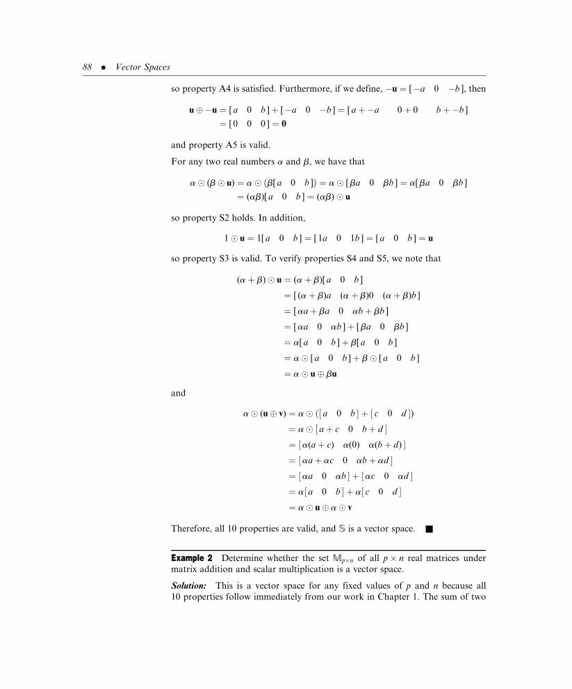
so property A4 is satisfied. Furthermore, if we define, �u ¼ [�a 0 �b ], then
u��u ¼ [ a 0 b ]þ [�a 0 �b ] ¼ [ aþ�a 0þ 0 bþ�b ]
¼ [ 0 0 0 ] ¼ 0
and property A5 is valid.
For any two real numbers a and b, we have that
a� (b� u) ¼ a� b[ a 0 b ]ð Þ ¼ a� [ ba 0 bb ] ¼ a[ ba 0 bb ]
¼ (ab)[ a 0 b ] ¼ (ab)� u
so property S2 holds. In addition,
1� u ¼ 1[ a 0 b ] ¼ [ 1a 0 1b ] ¼ [ a 0 b ] ¼ u
so property S3 is valid. To verify properties S4 and S5, we note that
(aþ b)� u ¼ (aþ b)[ a 0 b ]
¼ [ (aþ b)a (aþ b)0 (aþ b)b ]
¼ [ aaþ ba 0 abþ bb ]
¼ [ aa 0 ab ]þ [ ba 0 bb ]
¼ a[ a 0 b ]þ b[ a 0 b ]
¼ a� [ a 0 b ]þ b� [ a 0 b ]
¼ a� u� bu
and
a� (u� v) ¼ a� a 0 b½ � þ c 0 d½ �ð )
¼ a� aþ c 0 bþ d½ �¼ a(aþ c) a(0) a(bþ d)½ �¼ aaþ ac 0 abþ ad½ �¼ aa 0 ab½ � þ ac 0 ad½ �¼ a a 0 b½ � þ a c 0 d½ �¼ a� u� a� v
Therefore, all 10 properties are valid, and S is a vector space. &
Example 2 Determine whether the set Mp�n of all p� n real matrices under
matrix addition and scalar multiplication is a vector space.
Solution: This is a vector space for any fixed values of p and n because all
10 properties follow immediately from our work in Chapter 1. The sum of two
88 . Vector Spaces

real p� n matrices is again a matrix of the same order, as is the product of a
real number with a real matrix of this order. Thus, properties A1 and S1 are
satisfied. Properties A2 through A4 are precisely Theorem 1 in Section 1.1 and
Equation (1.5). If A ¼ [aij], then �A ¼ [� aij ] is another element in the set and
A��A ¼ [aij]þ [� aij ] ¼ (aij þ�aij)� �
¼ 0
which verifies property A5. Properties S2, S4, and S5 are Theorem 2 in Section
1.1. Property S3 is immediate from the definition of scalar multiplication. &
It follows from Example 2 that the set of all real 3� 3 matrices ( p ¼ n ¼ 3) is
a vector space, as is M2�6, the set of all real 2� 6 matrices ( p ¼ 2 and n ¼ 6).
Also, Rn is a vector space, for any positive integer n, because Rn is M1�n when we
take Rn to be the set of all n-dimensional real row matrices, and Rn is Mn�1 when
we take Rn to be the set of all n-dimensional real column matrices.
Example 3 Determine whether the set of all 2� 2 real matrices is a vector space
under regular scalar multiplication but with vector addition defined to be matrix
multiplication. That is,
u� v ¼ uv
Solution: This is not a vector space because it does not satisfy property A2.
In particular,
1 2
3 4
� ��
5 6
7 8
� �¼
1 2
3 4
� �5 6
7 8
� �¼
19 22
43 50
� �
6¼23 34
31 46
� �¼
5 6
7 8
� �1 2
3 4
� �¼
5 6
7 8
� ��
1 2
3 4
� �&
We use the � symbol to emphasize that vector addition may be nonstandard, as
it is in Example 3. The notation denotes a well-defined process for combining
two vectors together, regardless of how unconventional that process may be.
Generally, vector addition is standard, and many writers discard the � notation
in favor of the more conventional þ symbol whenever a standard addition is in
effect. We shall, too, in later sections. For now, however, we want to stress that
a vector space does not require a standard vector addition, only a well-defined
operation for combining two vectors that satisfies the properties listed in Defin-
ition 1, so we shall retain the � notation a while longer.
Example 4 Redo Example 3 with the matrices restricted to being diagonal.
Solution: Diagonal matrices do commute under matrix multiplication, hence
property A2 is now satisfied. The set is closed under vector addition, because the
product of 2� 2 diagonal matrices is again a diagonal matrix. Property A3 also
holds, because matrix multiplication is associative. With vector addition defined
The set Mp�n of all
p� n real matrices
under matrix
addition and scalar
multiplication is a
vector space.
The set Rn of
n-tuples under
standard addition
and scalar
multiplication for
n-tuples is a vector
space.
The symbol �emphasizes that
vector addition may
be nonstandard.
2.1 Vectors . 89
to be matrix multiplication, the zero vector becomes the 2� 2 identity matrix; for
any matrix A in the set, A� 0 ¼ AI ¼ A. To verify property A5, we must show
that every real diagonal matrix A has an additive inverse �A with the property
A��A ¼ 0. Given that we have just identified the zero vector to be the identity
matrix and vector addition to be matrix multiplication, the statement
A��A ¼ 0 is equivalent to the statement A(� A) ¼ I. Property A5 is valid if
and only if every matrix in the set has an inverse, in which case we take
�A ¼ A�1. But, a diagonal matrix with at least one 0 on its main diagonal
does not have an inverse. In particular the matrix,
A ¼ 1 0
0 0
� �
has no inverse. Thus, property A5 does not hold in general, and the given set is
not a vector space. &
Example 5 Redo Example 3 with the matrices restricted to being diagonal and
all elements on the main diagonal restricted to being nonzero.
Solution: Repeating the reasoning used in Example 4, we find that properties
A1–A5 are satisfied for this set. This set, however, is not closed under scalar
multiplication. Whenever we multiply a matrix in the set by the zero scalar,
we get
0� A ¼ 0A ¼ 0 0
0 0
� �
which is no longer a diagonal matrix with nonzero elements on the main
diagonal and, therefore, not an element of the original set. Thus, the given set
is not a vector space. &
Example 6 Determine whether the set of nth degree polynomials in the
variable t with real coefficients is a vector space under standard addition and
scalar multiplication for polynomials if the scalars are restricted also to being
real.
Solution: Arbitrary vectors u and v in this set are polynomials of the form
u ¼ antn þ an�1t
n�1 þ � � � þ a1tþ a0
v ¼ bntn þ bn�1t
n�1 þ � � � þ b1tþ b0
with aj and bj ( j ¼ 0, 1, . . . , n) all real, and both an and bn nonzero. Here,
u� v ¼ (antn þ an�1t
n�1 þ � � � þ a1tþ a0)
þ (bntn þ bn� 1tn�1 þ � � � þ b1tþ b0)
¼ (an þ bn)tn þ (an�1 þ bn�1)t
n�1 þ � � � þ (a1 þ b1)tþ (a0 þ b0)
90 . Vector Spaces

Note that when an ¼ �bn, u� v is no longer an nth degree polynomial, but rather
a polynomial of degree less than n, which is not an element of the given set. Thus,
the set is not closed under vector addition and is not a vector space. &
Example 7 Determine whether the set Pn containing the identically zero
polynomial and all polynomials of degree n or less in the variable t with real
coefficients is a vector space under standard addition and scalar multiplication
for polynomials, if the scalars also are restricted to being real.
Solution: If u 2 Pn and v 2 Pn, then u and v have the form
u ¼ antn þ an�1t
n�1 þ � � � þ a1tþ a0
v ¼ bntn þ bn�1t
n�1 þ � � � þ b1tþ b0
with aj and bj ( j ¼ 0, 1, . . . , n) real and possibly 0. Using the results of Example
6, we see that the sum of two polynomials of degree n or less is either another
polynomial of the same type or the zero polynomial when u and v have their
corresponding coefficients equal in absolute value but opposite in sign. Thus,
property A1 is satisfied. If we define the zero vector to be the zero polynomial,
then
u� 0 ¼ (antn þ an�1t
n�1 þ � � � þ a1tþ a0)
þ (0tn þ 0tn�1 þ � � � þ 0tþ 0)
¼ (an þ 0)tn þ (an�1 þ 0)tn�1 þ � � � þ (a1 þ 0)tþ (a0 þ 0)
¼ u
Thus, property A4 is satisfied. Setting
u ¼ �antn � an�1t
n�1 � � � � � a1t� a0
we note that property A5 is also satisfied. Now,
u� v ¼ (antn þ an�1t
n�1 þ � � � þ a1tþ a0)
þ (bntn þ bn�1t
n�1 þ � � � þ b1tþ b0)
¼ (an þ bn)tn þ (an�1 þ bn�1)t
n�1 þ � � � þ (a1 þ b1)tþ (a0 þ b0)
¼ (bn þ an)tn þ (bn�1 þ an�1)t
n�1 þ � � � þ (b1 þ a1)tþ (b0 þ a0)
¼ (bntn þ bn�1t
n�1 þ � � � þ b1tþ b0)
þ (antn þ an�1t
n�1 þ � � � þ a1tþ a0)
¼ v� u
so property A2 is satisfied. Property A3 is verified in a similar manner. For any
real number a, we have
2.1 Vectors . 91
a� u ¼ a(antþ an�1tn�1 þ � � � þ a1tþ a0)
¼ (aan)tþ (aan�1)tn�1 þ � � � þ (aa1)tþ (aa0)
which is again an element in the original set, so the set is closed under scalar
multiplication. Setting a ¼ 1 in the preceding equation also verifies property S3.
The remaining three properties follow in a straightforward manner, so Pn is a
vector space. &
Example 8 Determine whether the set of two-dimensional column matrices with
all components real and equal is a vector space under regular addition but with
scalar multiplication defined as
a� a
b
� �¼ �aa
�ab
� �
Solution: Following convention, the scalars are assumed to be real numbers.
Since column matrices are matrices, it follows from our work in Chapter 1 that
properties A1 through A5 hold. It is clear from the definition of scalar multipli-
cation that the set is closed under this operation; the result of multiplying
a real two-dimensional column matrix by a real number is again a real two-
dimensional column matrix. To check property S2, we note that for any two real
numbers a and b and for any vector
u ¼ a
b
� �
we have
(ab)� u ¼ (ab)� a
b
� �¼ �(ab)a
�(ab)b
� �¼ �aba
�abb
� �
while
a� (b� u) ¼ a� b� a
b
� �� �¼ a� �ba
�bb
� �¼ (� a)(� ba)
(� a)(� bb)
� �¼ aba
abb
� �
These two expressions are not equal whenever a and b are nonzero, so property
S2 does not hold and the given set is not a vector space.
Property S3 is also violated with this scalar multiplication. For any vector
u ¼ a
b
� �
we have
The set Pn of all
polynomials of
degree less than or
equal to n, including
the identically zero
polynomial, under
normal addition and
scalar multiplication
for polynomials is a
vector space.
92 . Vector Spaces

1� u ¼ 1� a
b
� �¼ �a
�b
� �6¼ u
Thus, we conclude again that the given set is not a vector space. &
We use the � symbol to emphasize that scalar multiplication may be nonstan-
dard, as it was in Example 8. The � symbol denotes a well-defined process for
combining a scalar with a vector, regardless of how unconventional the process
may be. In truth, scalar multiplication is generally quite standard, and many
writers discard the � notation whenever it is in effect. We shall, too, in later
sections. For now, however, we want to retain this notation to stress that a vector
space does not require a standard scalar multiplication, only a well-defined
process for combining scalars and vectors that satisfies properties S1 through S5.
Example 9 Determine whether the set of three-dimensional row matrices with
all components real and equal is a vector space under regular addition and scalar
multiplication if the scalars are complex numbers.
Solution: An arbitrary vector in this set has the form u ¼ [ a a a ], where a is
real. This is not a vector space, because the set violates property S1. In particular,
if a is any complex number with a nonzero imaginary part, then a� u does not
have real components. For instance, with a ¼ 3i and u ¼ [ 1 1 1 ], we have
a� u ¼ (3i) [ 1 1 1 ] ¼ [ 3i 3i 3i ]
which is not a real-valued vector; the components of the row matrix are complex,
not real. Thus, the original set is not closed under scalar multiplication. The
reader can verify that all the other properties given in Definition 1 are applicable.
However, as soon as we find one property that is not satisfied, we can immedi-
ately conclude the given set is not a vector space. &
The purpose of defining a vector space in the abstract is to create a single
mathematical structure that embodies the characteristics of many different
well-known sets, and then to develop facts about each of those sets simultane-
ously by studying the abstract structure. If a fact is true for vector spaces in
general, then that fact is true for Mp�n, the set of all p� n real matrices under
regular matrix addition and scalar multiplication, as well as Rn and Pn, the set of
all polynomials of degree less than or equal to n including the zero polynomial,
and any other set we may subsequently show is a vector set.
We first inquire about the zero vector. Does it have properties normally associ-
ated with the word zero? If we multiply the zero vector by a nonzero scalar, must
the result be the zero vector again? If we multiply any vector by the number 0, is
the result the zero vector? The answer in both cases is affirmative, but both
results must be proven. We cannot just take them for granted! The zero vector is
not the number 0, and there is no reason to expect (although one might hope)
that facts about the number 0 are transferable to other structures that just
happen to have the word zero as part of their name.
The symbol �emphasizes that
scalar multiplication
may be
nonstandard.
2.1 Vectors . 93

" Theorem 1. For any vector u in a vector space V, 0� u ¼ 0: 3
Proof: Because a vector space is closed under scalar multiplication, we know
that 0� u is a vector in V (whether it is the zero vector is still to be determined).
As a consequence of property A5, 0� u must possess an additive inverse,
denoted by �0� u, such that
(0� u)� (� 0� u) ¼ 0 (2:1)
Furthermore,
0� u ¼ (0þ 0)� u A property of the number 0
¼ 0� u� 0� u Property S4 of vector spaces
If we add the vector �0� u to each side of this last equation, we get
0� u��0� u ¼ (0� u� 0� u)��0� u
0 ¼ (0� u� 0� u)��0� u From Eq: (2:1)
0 ¼ 0� u� (0� u��0� u) Property A3
0 ¼ (0� u)� 0 From Eq: (2:1)
0 ¼ 0� u Property A4
which proves Theorem 1 using just the properties of a vector space. &
" Theorem 2. In any vector space V, a� 0 ¼ 0, for every scalar a: 3
Proof: 0 2 V, hence a� 0 2 V, because a vector space is closed under scalar
multiplication. It follows from property A5 that a� 0 has an additive inverse,
denoted by �a� 0, such that
(a� 0)� (� a� 0) ¼ 0 (2:2)
Furthermore,
a� 0 ¼ a� (0� 0) Property A4
¼ a� 0� a� 0 Property S5
Adding �a� 0 to both sides of this last equation, we get
94 . Vector Spaces

a� 0��a� 0 ¼ (a� 0� a� 0)��a� 0
0 ¼ (a� 0� a� 0)��a� 0 From Eq: (2:2)
0 ¼ a� 0� (a� 0��a� 0) Property A3
0 ¼ (a� 0)� 0 From Eq: (2:2)
0 ¼ a� 0 Property A4
Thus, Theorem 2 follows directly from the properties of a vector space. &
Property A4 asserts that every vector space has a zero vector, and property
A5 assures us that every vector in a vector space V has an additive inverse.
Neither property indicates whether there is only one zero element or many
or whether a vector can have more than one additive inverse. The next two
theorems do.
" Theorem 3. The additive inverse of any vector v in a vector space V is
unique. 3
Proof: Let v1 and v2 denote additive inverses of the same vector v. Then,
v� v1 ¼ 0 (2:3)
v� v2 ¼ 0 (2:4)
It now follows that
v1 ¼ v1 � 0 Property A4
¼ v1 � (v� v2) From Eq:(2:4)
¼ (v1 � v)� v2 Property A3
¼ (v� v1)� v2 Property A2
¼ 0� v2 From Eq:(2:3)
¼ v2 � 0 Property A2
¼ v2 Property A4
" Theorem 4. The zero vector in a vector space V is unique. 3
Proof: This proof is similar to the previous one and is left as an exercise for the
reader. (See Problem 34.)
2.1 Vectors . 95

" Theorem 5. For any vector w in a vector space V, � 1� w ¼ �w. 3
Proof: We need to show that �1� w is the additive inverse of w. First,
(� 1� w)� w ¼ (� 1� w)� (1� w) Property S3
¼ (� 1þ 1)� w Property S5
¼ 0� w Property of real numbers
¼ 0 Theorem 1
Therefore, �1� w is an additive inverse of w. By definition, �w is an additive
inverse of w, and because additive inverses are unique (Theorem 3), it follows
that �1� w ¼ �w.
" Theorem 6. For any vector w in a vector space V, � (� w) ¼ w. 3
Proof: By definition, �w is the additive inverse of w. It then follows that w is
the additive inverse of �w (see Problem 33). Furthermore,
�w��(� w) ¼ �1� w��(� w) Theorem 5
¼ �1� w��1� (� w) Theorem 5
¼ �1� (w��w) Property S5
¼ �1� 0 Property A5
¼ 0 Theorem 2
Therefore, �(� w) is an additive inverse of �w. Since w is also an additive
inverse of �w, it follows from Theorem 3 that the two are equal. &
" Theorem 7. Let a be a scalar and u a vector in a vector space V.
If a� u ¼ 0, then either a ¼ 0 or u ¼ 0. 3
Proof: We are given
a� u ¼ 0 (2:5)
Now either a is 0 or it is not. If a is 0, the theorem is proven. If a is not 0, we
form the scalar 1=a and then multiply Eq. (2.5) by 1=a, obtaining
96 . Vector Spaces

(1=a)� (a� u) ¼ (1=a)� 0
(1=a)� (a� u) ¼ 0 Theorem 2
1
aa
� �� u ¼ 0 Property S2
1� u ¼ 0 Property of numbers
u ¼ 0 & Property S3
Problems 2.1
In Problems 1 through 32 a set of objects is given together with a definition for vector
addition and scalar multiplication. Determine which are vector spaces, and for those that
are not, identify at least one property that fails to hold.
(1)a b
c d
� �� �2M2�2jb ¼ 0:g under standard matrix addition and scalar multiplication.
(2)a b
c d
� �� �2M2�2jc ¼ 1:g under standard matrix addition and scalar multiplication.
(3) The set of all 2� 2 real matrices A ¼ [aij ] with a11 ¼ �a22 under standard matrix
addition and scalar multiplication.
(4) The set of all 3� 3 real upper triangular matrices under standard matrix addition
and scalar multiplication.
(5) The set of all 3� 3 real lower triangular matrices of the form
1 0 0
a 1 0
b c 1
24
35
under standard matrix addition and scalar multiplication.
(6) f[ a b � 2 R2jaþ b ¼ 2g under standard matrix addition and scalar multiplication.
(7) f[ a b � 2 R2ja ¼ bg under standard matrix addition and scalar multiplication.
(8) All 2-tuples representing points in the first quadrant of the plane, including the
origin, under standard addition and scalar multiplication for 2-tuples.
(9) All 2-tuples representing points in the first and third quadrants of the plane,
including the origin, under standard addition and scalar multiplication for 2-tuples.
(10) All 2-tuples representing points in the plane that are on the straight line y ¼ �2x
under standard addition and scalar multiplication for 2-tuples.
(11) All 2-tuples representing points in the plane that are on the straight line
y ¼ �2xþ 1, under standard addition and scalar multiplication for 2-tuples.
2.1 Vectors . 97

(12) All 2-tuples representing points in the plane that are on the parabola y ¼ x2, under
standard addition and scalar multiplication for 2-tuples.
(13) The set consisting of the single element 0 with vector addition and scalar multipli-
cation defined as 0� 0 ¼ 0 and a� 0 ¼ 0 for any real number a.
(14) The set of all real two-dimensional row matrices f[ a b ]g with standard matrix
addition but scalar multiplication defined as a� [ a b ] ¼ [ 0 0 ].
(15) The set of all real two-dimensional row matrices f[ a b ]g with standard matrix
addition but scalar multiplication defined as a� [ a b ] ¼ [ 0 ab ].
(16) The set of all real two-dimensional row matrices f[ a b ]g with standard matrix
addition but scalar multiplication defined as a� [ a b ] ¼ [ 2aa 2ab ].
(17) The set of all real two-dimensional row matrices f[ a b ]g with standard matrix
addition but scalar multiplication defined as a� [ a b ] ¼ [ 5a 5b ].
(18) The set of all real three-dimensional row matrices f[ a b c ]g with standard scalar
multiplication but vector addition defined as
[ a b c ]� [ x y z ] ¼ [ aþ x bþ yþ 1 cþ z ]
(19) The set of all real three-dimensional row matrices f[ a b c ]g with standard scalar
multiplication but vector addition defined as
[ a b c ]� [ x y z ] ¼ [ a bþ y c ]
(20) The set of all real three-dimensional row matrices f[ a b c ]g with standard
matrix addition but scalar multiplication defined as a� [ a b c ] ¼ [ aa ab 1 ].
(21) The set of all real three-dimensional row matrices f[ a b c ]g with positive com-
ponents under standard matrix addition but scalar multiplication defined as
a� [ a b c ] ¼ [ aa ba ca ]
(22) The set of all real numbers (by convention, the scalars are also real numbers) with
a� b ¼ a� b ¼ ab, the standard multiplication of numbers.
(23) The set of all positive real numbers with a� b ¼ ab, the standard multiplication of
numbers, and a� b ¼ ab.
(24) The set of all solutions of the homogeneous set of linear equations Ax ¼ 0, under
standard matrix addition and scalar multiplication.
(25) The set of all solutions of the set of linear equations Ax ¼ b, b 6¼ 0, under standard
matrix addition and scalar multiplication.
(26) fp(t) 2 P3j p(0) ¼ 0g under standard addition and scalar multiplication of polyno-
mials.
(27) All polynomials in P3, under standard addition and scalar multiplication, satisfying
the constraint that the graph of each polynomial is above the t-axis on the interval
1 < t < 3.
(28) The set of all real-valued continuous functions on the interval [�1, 1 ] under
standard function addition and scalar multiplication, usually denoted as C[� 1, 1].
98 . Vector Spaces
(29) The set of all real-valued continuous functions on the interval [ 0, 1 ] under
standard function addition and scalar multiplication, usually denoted as C[0, 1].
(30) The set of all real-valued continuous functions, ff (t)g, on the interval [ 0, 1 ]
under standard scalar multiplication but with vector addition defined as
f1(t)� f2(t) ¼ f1(t)f2(t), the standard product of functions.
(31) The set of all real-valued continuous functions, ff (t)g, on the interval [ 0, 1 ]
under standard scalar multiplication but with vector addition defined as
f1(t)� f2(t) ¼ f1(f2(t)), the standard composition of functions.
(32) The set of all solutions of the differential equation y00 þ y ¼ 0 under standard
function addition and the multiplication of a function by a scalar.
(33) Let w be a vector in a vector space V. Prove that if �w is the additive inverse of w
then the reverse is also true: w is the additive inverse of �w.
(34) Prove Theorem 4.
(35) Prove that v� (u� v) ¼ u if u� v is shorthand for u��v.
(36) Prove that if u� v ¼ u� w, then v ¼ w.
(37) Prove that u� u ¼ 2u if 2u is shorthand for 2� u.
(38) Prove that the only solution to the equation u� u ¼ 2v is u ¼ v.
(39) Prove that if u 6¼ 0 and a� u ¼ b� u, then a ¼ b.
(40) Prove that the additive inverse of the zero vector is the zero vector.
2.2 SUBSPACES
To show that a set of objects S is a vector space, we must verify that all
10 properties of a vector space are satisfied, the 5 properties involving vector
addition and the 5 properties involving scalar multiplication. This process,
however, can be shortened considerably if the set of objects is a subset of
a known vector space V. Then, instead of 10 properties, we need only verify the
2 closure properties, because the other 8 properties follow immediately from
these 2 and the fact that S is a subset of a known vector space.
We define a nonempty subset S of a vector space V as a subspace of V if S is itself
a vector space under the same operations of vector addition and scalar multipli-
cation defined on V.
" Theorem 1. Let S be a nonempty subset of a vector space V with
operations � and �. S is a subspace of V if and only if the following
two closure conditions hold:
(i) Closure under addition: If u 2 S and v 2 S, then u� v 2 S.
(ii) Closure under scalar multiplication: If u 2 S and a is any
scalar, then a� u 2 S. 3
A subspace of a
vector space V is a
subset of V that is a
vector space in its
own right.
2.2 Subspaces . 99

Proof: If S is a vector space, then it must satisfy all 10 properties of a vector
space, in particular the closure properties defined by conditions (i) and (ii). Thus,
if S is a vector space, then (i) and (ii) are satisfied.
We now show the converse: If conditions (i) and (ii) are satisfied, then S is
a vector space; that is, all 10 properties of a vector space specified in Definition 1
of section 2.1 follow from the closure properties and the fact that S is a subset of
a known vector space V. Conditions (i) and (ii) are precisely Properties A1 and
S1. Properties A2, A3, and S2 through S5 follow for elements in S because these
elements are also in V and V is known to be a vector space whose elements satisfy
all the properties of a vector space. In particular, to verify Property A2, we let
u and v denote arbitrary elements in S. Because S is a subset of V, it follows that
u and v are in V. Because V is a vector space, we have u� v ¼ v� u. To verify S3,
we let u again denote an arbitrary element in S. Because S is a subset of V, it
follows that u is an element of V. Because V is a vector space, we have 1� u ¼ u.
All that remains is to verify that the zero vector and additive inverses of elements
in S are themselves members of S. Because S is nonempty, it must contain at
least one element, which we denote as u. Then, for the zero scalar, 0, we know
that 0� u is in S, as a result of condition (ii), and this vector is the zero vector as
a result of Theorem 1 of the previous section. Thus, Property A4 is satisfied. If u
is an element of S; then the product �1� u is also an element of S, as a result of
condition (ii); it follows from Theorem 5 of the previous section that �1� u is
the additive inverse of u, so Property A5 is also satisfied.
" Convention: For the remainder of this book, we drop the � and �symbols in favor of the traditional sum symbol (þ ) and scalar multipli-
cation denoted by juxtaposition. All vector spaces will involve standard
vector addition and scalar multiplication, unless noted otherwise. 3
We use Theorem 1 to significantly shorten the work required to show that some
sets are vector spaces!
Example 1 Determine whethera b
c d
� �2M2�2jb ¼ c ¼ 0
� �is a vector space
under standard matrix addition and scalar multiplication.
Solution: The set S of 2� 2 real matrices with zeros in the 1-2 and 2-1 positions
is a subset of M2�2, and M2�2 is a vector space (see Example 4 in Section 2.1 with
p ¼ n ¼ 2). Thus, Theorem 1 is applicable, and instead of verifying all 10 prop-
erties of a vector space, we need only verify closure in S under matrix addition
and scalar multiplication.
Arbitrary elements u and v in S have the form
u ¼ a 0
0 b
� �and v ¼ c 0
0 d
� �
100 . Vector Spaces

for any real numbers a, b, c, and d. Here
uþ v ¼ aþ c 0
0 bþ d
� �
and for any real scalar a,
au ¼ aa 0
0 ab
� �
Because these matrices are again elements in S, each having zeros in their 1-2 and
2-1 positions, it follows from Theorem 1 that S is a subspace of M2�2. The set
S is therefore a vector space. &
Example 2 Determine whether the set S ¼ f[ x y z ] 2 R3jy ¼ 0g is a vector
space under standard matrix addition and scalar multiplication.
Solution: We first observe that S is a subset of R3, considered as row matrices,
which we know is a vector space from our work in Section 2.1. Thus, Theorem 1
is applicable. Arbitrary elements u and v in S have the form
u ¼ [ a 0 b ] and v ¼ [ c 0 d ]
It follows that
uþ v ¼ [ aþ c 0 bþ d ] 2 S
and for any real scalar a,
au ¼ [ aa 0 ab ] 2 S
Thus, S is closed under addition and scalar multiplication, and it follows from
Theorem 1 that S is a subspace of R3. The set S is therefore a vector space. &
Compare Example 2 to Example 1 of Section 2.1. In both, we were asked
to prove that the same set is a vector space. In Section 2.1, we did this by
verifying all 10 properties of a vector space; in Example 2, we verified the
2 properties of a subspace. Clearly it is simpler to verify 2 properties than 10;
thus, it is simpler to show that a set is vector space by showing it is a subspace
rather than demonstrating directly that the set is a vector space. To do so,
however, we must recognize that the given set is a subset of known vector
space, in this case R3.
The subspace in Example 2 has an interesting graphical representation. R3, the
set of all 3-tuples, is represented geometrically by all points in three-space. The
set S in Example 2 is the set of all points in R3 having a second component of 0.
If a set is a subset of
a known vector
space, then the
simplest way to
show the set is a
vector space is to
show the set is a
subspace.
2.2 Subspaces . 101
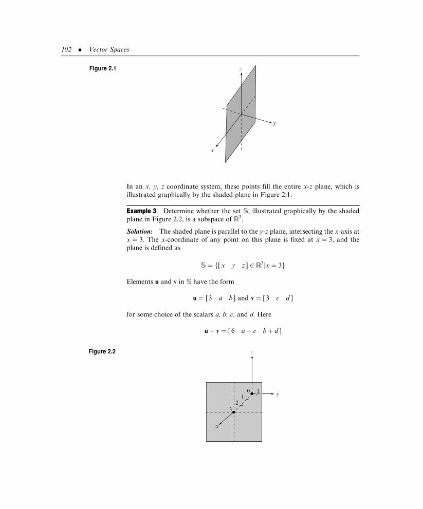
In an x, y, z coordinate system, these points fill the entire x-z plane, which is
illustrated graphically by the shaded plane in Figure 2.1.
Example 3 Determine whether the set S, illustrated graphically by the shaded
plane in Figure 2.2, is a subspace of R3.
Solution: The shaded plane is parallel to the y-z plane, intersecting the x-axis at
x ¼ 3. The x-coordinate of any point on this plane is fixed at x ¼ 3, and the
plane is defined as
S ¼ f[ x y z ] 2 R3jx ¼ 3g
Elements u and v in S have the form
u ¼ [ 3 a b ] and v ¼ [ 3 c d ]
for some choice of the scalars a, b, c, and d. Here
uþ v ¼ [ 6 aþ c bþ d ]
Figure 2.1
x
y
z
Figure 2.2 z
y01
1
23
x
102 . Vector Spaces

which is not an element of S because its first component is not 3. Condition (i) of
Theorem 1 is violated. The set S is not closed under addition and, therefore, is
not a subspace. &
As an alternative solution to Example 3, we note that the set S does not contain the
zero vector, and therefore cannot be a vector space. The zero vector in R3 is
0 ¼ [ 0 0 0 ], and this vector is clearly not in S because all elements in S have
a first component of 3. Often we can determine by inspection whether the zero
vector of a vector space is included in a given subset. If the zero vector is not
included, we may conclude immediately that the subset is not a vector space and,
therefore, not a subspace. If the zero vector is part of the set, then the two closure
properties must be verified before one can determine whether the given set is a
subspace.
One simple subspace associated with any vector space is the following:
" Theorem 2. For any vector space V, the subset containing only the zero
vector is a subspace. 3
Proof: It follows from the definition of a zero vector that 0þ 0 ¼ 0. It also
follows from Theorem 2 of Section 2.1 that a0 ¼ 0 for any scalar a. Both closure
conditions of Theorem 1 are satisfied, and the set S containing just the single
element 0 is a subspace. &
Example 4 Determine whether the set S ¼ f[ a 2a 4a ]ja is a real numbergis a subspace of R3.
Solution: Setting a ¼ 0, we see that the zero vector, 0 ¼ [ 0 0 0 ], of R3 is an
element of S, so we can make no conclusion a priori about S as a subspace. We
must apply Theorem 1 directly. Elements u and v in S have the form
u ¼ [ t 2t 4t ] and v ¼ [ s 2s 4s ]
for some choice of the scalars s and t. Therefore,
uþ v ¼ [ tþ s 2tþ 2s 4tþ 4s ]
¼ [ (tþ s) 2(tþ s) 4(tþ s) ] 2 S
and for any real scalar a,
au ¼ [ at a(2t) a(4t) ]
¼ [ (at) 2(at) 4(at) ] 2 S
Because S is closed under vector addition and scalar multiplication, it follows
from Theorem 1 that S is a subspace of R3. &
If a subset of a
vector space does
not include the zero
vector, that subset
cannot be a
subspace.
2.2 Subspaces . 103

The subspace in Example 4 also has an interesting graphical representation.
If we rewrite an arbitrary vector u as
u ¼ [ t 2t 4t ] ¼ t[ 1 2 4 ]
we see that every vector is a scalar multiple of the directed line segment having its
tail at the origin and its tip at the point (1, 2, 4). Because t can be any real
number, zero, positive or negative, we can reach any point on the line that
contains this directed line segment. Thus, the subspace S is represented graph-
ically by the straight line in R3 illustrated in Figure 2.3.
As a result of Examples 2 through 4 and Theorem 2, one might suspect that a
proper subset S of R3 is a subspace if and only if S is the zero vector or else the
graph of S is either a straight line through the origin or a plane that contains the
origin. This is indeed the case as we shall prove in Section 2.4.
The two conditions specified in Theorem 1 can be collapsed into a single
condition.
" Theorem 3. A nonempty subset S of a vector space V is a subspace of V
if and only if whenever u and v are any two elements in S and a and b are
any two scalars, then
auþ bv (2:6)
is also in S. 3
Proof: If S is a subspace, then it must satisfy the two conditions of Theorem 1.
In particular, if u is an element of S and a a scalar, then au is in S as
Figure 2.3
(1, 2, 0)
(1, 2, 4)
5
z
x
y
4
3
3
2
2
1
1
1 2 3 4
u
line that contains u
Lines through the
origin and planes
that contain the
origin are subspaces
of R3.
104 . Vector Spaces

a consequence of condition (ii). Similarly, bv must be an element of S whenever v
is an element and b is a scalar. Knowing that au and bv are two elements in S, we
may conclude that their sum, given by equation (2.6), is also in S as a conse-
quence of condition (i).
Conversely, if equation (2.6) is an element in S for all values of the scalars a and
b, then condition (i) of Theorem 1 follows by setting a ¼ b ¼ 1. Condition (ii)
follows by setting b ¼ 0 and leaving a arbitrary. &
Example 5 Determine whether S ¼ fp(t) 2 P2j p(2) ¼ 1g is a subspace of P2.
Solution: P2 is a vector space (see Example 7 of Section 2.1 with n ¼ 2). The
zero vector 0 in P2 has the property 0(t) ¼ 0 for all real values of t. Thus,
0(2) ¼ 0 6¼ 1, the zero vector is not in S, and S is not a subspace. &
Example 6 Determine whether S ¼ fp(t) 2 P2j p(2) ¼ 0g is a subspace of P2.
Solution: Let u ¼ p and v ¼ q be any two polynomials in S. Then p(2) ¼ 0 and
q(2) ¼ 0. Set w ¼ auþ bv, for arbitrary values of the scalars a and b. Then w is
also a polynomial of degree two or less or the zero polynomial. Furthermore,
w(2) ¼ (apþ bq)(2) ¼ ap(2)þ bq(2) ¼ a0þ b0 ¼ 0,
so w is also an element of S. It follows from Theorem 3 that S is a subspace
of P n. &
Expression (2.6) in Theorem 3 is a special case of a linear combination. We say
that a vector u in a vector space V is a linear combination of the vectors
v1, v2, . . . , vn in V if there exists scalars d1, d2, . . . , dn such that
u ¼ d1v1 þ d2v2 þ . . .þ dnvn (2:7)
Example 7 Determine whether u ¼ [ 1 2 3 ] is a linear combination of
v1 ¼ [ 1 1 1 ], v2 ¼ [ 2 4 0 ], and v3 ¼ [ 0 0 1 ]
Solution: These vectors are all in the vector space R3, considered as row
matrices. We seek scalars d1, d2, and d3 that satisfy the equation
[ 1 2 3 ] ¼ d1[ 1 1 1 ]þ d2[ 2 4 0 ]þ d3[ 0 0 1 ]
or
[ 1 2 3 ] ¼ [ d1 þ 2d2 d1 þ 4d2 d1 þ d3 ]
This last matrix equation is equivalent to the system of equations
A vector u is a linear
combination of
a finite number of
other vectors if u
can be written as
a sum of scalar
multiples of those
vectors.
2.2 Subspaces . 105

1 ¼ d1 þ 2d2
2 ¼ d1 þ 4d2
3 ¼ d1 þ d3
Using Gaussian elimination, we find that the only solution to this system is
d1 ¼ 0, d2 ¼ 1=2, and d3 ¼ 3. Thus,
[ 1 2 3 ] ¼ 0[ 1 1 1 ]þ 12[ 2 4 0 ]þ 3[ 0 0 1 ]
and the vector u ¼ [ 1 2 3 ] is a linear combination of the other three. &
Example 8 Determine whether u ¼ �1 0
2 4
� �is a linear combination of
v1 ¼1 1
2 2
� �and v2 ¼
3 2
3 5
� �
Solution: These vectors are in the vector space M2�2. We seek scalars d1 and d2
that satisfy the equation
�1 0
2 4
� �¼ d1
1 1
2 2
� �þ d2
3 2
3 5
� �(2:8)
or
�1 0
2 4
� �¼ d1 þ 3d2 d1 þ 2d2
2d1 þ 3d2 2d1 þ 5d2
� �
which is equivalent to the system of equations
�1 ¼ d1 þ 3d2
0 ¼ d1 þ 2d2
2 ¼ 2d1 þ 3d2
4 ¼ 2d1 þ 5d2
Using Gaussian elimination, we find that this system has no solution. There are
no values of d1 and d2 that satisfy (2.8), and, therefore, u is not a linear
combination of v1 and v2.
The set of all linear combinations of a finite set of vectors, S ¼ fv1, v2, . . . , vng, is
called the span of S, denoted as span fv1, v2, . . . , vng or simply span(S). Thus, the
span of the polynomial set ft2, t, 1g is P2 because every polynomial p(t) in P2 can
be written as
p(t) ¼ d1t2 þ d2tþ d3(1)
The span of a finite
number of vectors is
the set of all linear
combinations of
those vectors.
106 . Vector Spaces
for some choice of the scalars d1, d2, and d3. The span of the set f[ 1 0 0 0 ],
[ 0 1 0 0 ]g are all row-vectors of the form [ d1 d2 0 0 ] for any choice of
the real numbers d2 and d3.
The span of a finite set of vectors is useful because it is a subspace! Thus, we
create subspaces conveniently by forming all linear combinations of just a few
vectors.
" Theorem 4. The span of a set of vectors S ¼ fv1, v2, . . . , vng in a vector
space V is a subspace of V. 3
Proof: Let u and w be elements of span(S). Then
u ¼ d1v1 þ d2v2 þ . . .þ dnvn and w ¼ c1v1 þ c2v2 þ . . .þ cnvn
for some choice of the scalars d1 through dn and c1 through cn. It follows that
auþ bw ¼ a(d1v1 þ d2v2 þ . . .þ dnvn)þ b(c1v1 þ c2v2 þ . . .þ cnvn)
¼ (ad1)v1 þ (ad2)v2 þ . . .þ (adn)vn þ (bc1)v1 þ (bc2)v2 þ . . .þ (bcn)vn
¼ (ad1 þ bc1)v1 þ (ad2 þ bc2)v2 þ . . .þ (adn þ bcn)vn
Each quantity in parentheses on the right side of this last equation is
a combination of scalars of the form adj þ bcj (for j ¼ 1, 2, . . . , n) and is,
therefore, itself a scalar. Thus, auþ bw is a linear combination of the vectors
in S and a member of span(S). It follows from Theorem 3 that span(S) is a
subspace of V. &
Not only is the span(S) a subspace that includes the vectors in S, but it is the
smallest such subspace. We formalize this statement in the following theorem,
the proof of which is left as an exercise for the reader (see Problem 50).
" Theorem 5. If S ¼ fv1, v2, . . . , vng is a set of vectors in a vector space V
and if W is a subspace of V that contains all the vectors in S, then W
contains all the vectors in span(S). 3
Problems 2.2
In Problems 1 through 27, determine whether each set is a vector space.
(1) S ¼ f[ a b ] 2 R2ja ¼ 0g.
(2) S ¼ f[ a b ] 2 R2ja ¼ �bg.
(3) S ¼ f[ a b ] 2 R2jb ¼ �5ag.
(4) S ¼ f[ a b ] 2 R2jb ¼ aþ 3g.
2.2 Subspaces . 107
(5) S ¼ f[ a b ] 2 R2jb � ag.
(6) S ¼ f[ a b ] 2 R2ja ¼ b ¼ 0g.
(7) S ¼ f[ a b c ] 2 R3ja ¼ bg.
(8) S ¼ f[ a b c ] 2 R3jb ¼ 0g.
(9) S ¼ f[ a b c ] 2 R3ja ¼ bþ 1g.
(10) S ¼ f[ a b c ] 2 R3jc ¼ a� bg.
(11) S ¼ f[ a b c ] 2 R3jc ¼ abg.
(12) S ¼ f[ a b c ] 2 R3ja ¼ b and c ¼ 0g.
(13) S ¼ f[ a b c ] 2 R3jb ¼ 3a and c ¼ aþ 3g.
(14) S ¼ a 2a 0
0 a 2a
� �a is real
( )as a subset of M2�3.
(15)a b c
d e f
� �: 2M2�3
� c ¼ e ¼ f ¼ 0
�.
(16)a b c
d e f
� �: 2M2�3
� c ¼ e ¼ f ¼ 1
�.
(17) S ¼ 0 0 0
0 0 0
� �� �as a subset of M2�3.
(18) S ¼ fA 2M3�3jA is lower triangularg.
(19) S ¼ fA 2M3�3jA is a diagonal matrixg.
(20) S ¼a a2 a3
a2 a a2
a3 a2 a
24
35
8<:
a is real
9=; as a subset of M3�3.
(21) S ¼ fA 2M2�2jA is invertibleg.
(22) S ¼ fA 2M2�2jA is singularg.
(23) S ¼ fat2 þ btþ c 2 P2jb ¼ 0g.
(24) S ¼ fp(t) 2 P2jp(3)� 2p(1) ¼ 4g.
(25) S ¼ ff (t) 2 C[0, 1]þ f (t) > 0g. (C[0, 1] is defined in Problem 29 of Section 2.1.)
(26) S ¼ ff (t) 2 C[� 1, 1]jf (� t) ¼ f (t)g. (C[� 1, 1] is defined in Problem 28 of
Section 2.2.)
(27) S ¼ ff (t) 2 C[� 1, 1]jf (� t) ¼ �f (t)g:
(28) Determine whether u is a linear combination of v1 ¼ [ 1 2 ] and v2 ¼ [ 3 6 ].
(a) u ¼ [ 2 4 ], (b) u ¼ [ 2 �4 ],
(c) u ¼ [�3 �6 ], (d) u ¼ [ 2 2 ].
(29) Determine which, if any, of the vectors u defined in the previous problem are in
spanfv1, v2g.
(30) Determine whether u is a linear combination of v1 ¼ [ 1 0 1 ] and
v2 ¼ [ 1 1 1 ].
108 . Vector Spaces
(a) u ¼ [ 3 2 3 ], (b) u ¼ [ 3 3 2 ],
(c) u ¼ [ 0 0 0 ], (d) u ¼ [ 0 1 1 ].
(31) Determine which, if any, of the vectors u defined in the previous problem
are in spanfv1, v2g.(32) Determine whether the following vectors are linear combinations of
v1 ¼1
0
0
2435, v2 ¼
1
1
0
2435, v3 ¼
1
1
1
2435:
(a)
1
0
1
2435, (b)
1
0
�1
24
35, (c)
2
2
0
2435,
(d)
2
2
4
2435, (e)
1
2
3
2435, (f)
2
�5
� �.
(33) Determine whether the following matrices are linear combinations of
A1 ¼1 0
0 0
� �, A2 ¼
0 1
0 0
� �, A3 ¼
1 1
1 0
� �:
(a)0 1
1 1
� �, (b)
1 2
3 0
� �, (c)
1 1
0 0
� �,
(d)0 0
0 0
� �, (e)
2 0
�2 0
� �, (f)
0 0
1 �1
� �.
(34) Determine which, if any, of the matrices given in parts (a) through (f) of the
previous problem are in spanfA1,A2, A3g.
(35) Determine whether the following polynomials are linear combinations of
ft3 þ t2, t3 þ t, t2 þ tg:
(a) t3 þ t2 þ t, (b) 2t3 � t, (c) 5t, (d) 2t2 þ 1.
(36) Find spanfv1, v2g for the vectors given in Problem 28.
(37) Find spanfA1,A2,A3g for the matrices given in Problem 33.
(38) Find spanfp1(t), p2(t), p3(t)g for the polynomial given in Problem 35.
(39) Describe the graph of all points in the set S described in Problem 3.
(40) Show that the set of points in the plane on a straight line passing through the origin
is a subspace of R2.
(41) Show that S as given in Problem 4 is the set of points in the plane on the graph of
the straight line y ¼ xþ 3. Describe a characteristic of this line that precludes S
from being a subspace.
2.2 Subspaces . 109

(42) Show that P2 is a subspace of P3. Generalize to Pm and Pn when m < n.
(43) Show that if u is a linear combination of the vectors v1, v2, . . . , vn and if each vi
(i ¼ 1, 2, . . . , n) is a linear combination of the vectors w1,w2, . . . , wm, then u can
also be expressed as a linear combination of w1,w2, . . . ,wm.
(44) Let A be an n� n matrix and both x and y n� 1 column matrices. Prove that if
y ¼ Ax, then y is a linear combination of the columns of A.
(45) Show that the set of solutions of the matrix equation Ax ¼ 0, where A is a p� n
matrix, is a subspace of Rn.
(46) Show that the set of solutions of the matrix equation Ax ¼ b, where A is a p� n
matrix, is not a subspace of Rn when b 6¼ 0.
(47) Prove that spanfu, vg ¼ spanfuþ v, u� vg.
(48) Prove that spanfu, v,wg ¼ spanfuþ v, vþ w, uþ wg.
(49) Prove that spanfu, v, 0g ¼ spanfu, vg.
(50) Prove Theorem 5.
2.3 LINEAR INDEPENDENCE
Most vector spaces contain infinitely many vectors. In particular, if u is a nonzero
vector of a vector space V and if the scalars are real numbers, then it follows
from the closure property of scalar multiplication that au 2 V for every real
number a. It is useful, therefore, to determine whether a vector space can be
completely characterized by just a few representatives. If so, we can describe
a vector space by its representatives. Instead of listing all the vectors in a vector
space, which are often infinitely many in number, we simplify the identification
of a vector space by listing only its representatives. We then use those represen-
tatives to study the entire vector space.
Efficiently characterizing a vector space by its representatives is one of the major
goals in linear algebra, where by efficiently we mean listing as few representatives
as possible. We devote this section and the next to determining properties that
such a set of representatives must possess.
A set of vectors fv1, v2, . . . , vng in a vector space V is linearly dependent if there
exist scalars, c1, c2, . . . , cn, not all zero, such that
c1v1 þ c2v2 þ . . .þ cnvn ¼ 0 (2:9)
The vectors are linearly independent if the only set of scalars that satisfies
equation (2.9) is the set c1 ¼ c2 ¼ . . . ¼ cn ¼ 0.
To test whether a given set of vectors is linearly independent, we first form vector
equation (2.9) and ask, ‘‘What values for the c’s satisfy this equation?’’ Clearly,
c1 ¼ c2 ¼ . . . ¼ cn ¼ 0 is a suitable set. If this is the only set of values that
The set of vectors
fv1, v2, . . . , vngis linearly
independent if the
only set of scalars
that satisfy
c1v1 þ c2v2
þ . . .þ cnvn ¼ 0
is c1 ¼ c2 ¼ . . .¼ cn ¼ 0.
110 . Vector Spaces

satisfies (2.9), then the vectors are linearly independent. If there exists a set of
values that is not all zero, then the vectors are linearly dependent.
It is not necessary for all the c’s to be different from zero for a set of vectors to be
linearly dependent. Consider the vectors v1 ¼ [ 1 2 ], v2 ¼ [ 1 4 ]; and
v3 ¼ [ 2 4 ]. The constants c1 ¼ 2, c2 ¼ 0; and c3 ¼ �1 is a set of scalars, not
all zero, such that c1v1 þ c2v2 þ c3v3 ¼ 0. Thus, this set is linearly dependent.
Example 1 Is the set f[ 1 2 ], [ 3 4 ]g in R2 linearly independent?
Solution: Here v1 ¼ [ 1 2 ], v2 ¼ [ 3 4 ]; and equation (2.9) becomes
c1[ 1 2 ]þ c2[ 3 4 ] ¼ [ 0 0 ]
This vector equation can be rewritten as
[ c1 2c1 ]þ [ 3c2 4c2 ] ¼ [ 0 0 ]
or as
[ c1 þ 3c2 2c1 þ 4c2 ] ¼ [ 0 0 ]
Equating components, we generate the system
c1 þ 3c2 ¼ 0
2c1 þ 4c2 ¼ 0
which has as its only c1 ¼ c2 ¼ 0. Consequently, the original set of vectors is
linearly independent. &
Example 2 Determine whether the set of column matrices in R3
2
6
�2
24
35,
3
1
2
2435,
8
16
�3
24
35
8<:
9=;
is linearly independent.
Solution: Equation (2.9) becomes
c1
2
6
�2
24
35þ c2
3
1
2
2435þ c3
8
16
�3
24
35 ¼
0
0
0
2435 (2:10)
which can be rewritten as
2.3 Linear Independence . 111

2c1
6c1
�2c1
24
35þ 3c2
c2
2c2
24
35þ 8c3
16c3
�3c3
24
35 ¼ 0
0
0
2435
or
2c1 þ 3c2 þ 8c3
6c1 þ c2 þ 16c3
�2c1 þ 2c2 � 3c3
24
35 ¼ 0
0
0
2435
This matrix equation is equivalent to the homogeneous system of equations
2c1 þ 3c2 þ 8c3 ¼ 0
6c1 þ c2 þ 16c3 ¼ 0
�2c1 þ 2c2 � 3c3 ¼ 0
Using Gaussian elimination, we find the solution to this system is c1 ¼ �2:5c3,
c2 ¼ �c3, c3 arbitrary. Setting c3 ¼ 2, we obtain c1 ¼ �5, c2 ¼ �2, c3 ¼ 2 as a
particular nonzero set of constants that satisfies equation (2.10). The original set
of vectors is linearly dependent. &
Example 3 Determine whether the set of matrices
1 1
0 0
� �,
0 1
0 1
� �,
0 0
1 1
� �,
1 0
1 1
� �,
1 1
0 1
� �� �
in M2�2 is linearly independent.
Solution: Equation (2.9) becomes
c11 1
0 0
� �þ c2
0 1
0 1
� �þ c3
0 0
1 1
� �þ c4
1 0
1 1
� �þ c5
1 1
0 1
� �¼ 0 0
0 0
� �
or
c1 þ c4 þ c5 c1 þ c2 þ c5
c3 þ c4 c2 þ c3 þ c4 þ c5
� �¼ 0 0
0 0
� �
which is equivalent to the homogeneous system of equations
c1 þ c4 þ c5 ¼ 0
c1c2 þ c5 ¼ 0
c3 þ c4 ¼ 0
c2 þ c3 þ c4 þ c5 ¼ 0
112 . Vector Spaces

This system has more unknowns than equations, so it follows from Theorem 3 of
Section 1.4 that there are infinitely many solutions, all but one of which are
nontrivial. Because nontrivial solutions exist to equation (2.9), the set of vectors
is linearly dependent. &
Example 4 Determine whether the set ft2 þ 2t� 3, t2 þ 5t, 2t2 � 4g of vectors in
P2 is linearly independent.
Solution: Equation (2.9) becomes
c1(t2 þ 2t� 3)þ c2(t
2 þ 5t)þ c3(2t2 � 4) ¼ 0
or
(c1 þ c2 þ 2c3)t2 þ (2c1 þ 5c2)tþ (� 3c1 � 4c3) ¼ 0t2 þ 0tþ 0
Equating coefficients of like powers of t, we generate the system of equations
c1 þ c2 þ 2c3 ¼ 0
2c1 þ 5c2 ¼ 0
�3c1 � 4c3 ¼ 0
Using Gaussian elimination, we find that this system admits only the trivial
solution c1 ¼ c2 ¼ c3 ¼ 0. The given set of vectors is linearly independent. &
The defining equations for linear combinations and linear dependence, (2.7) and
(2.9), are similar, so we should not be surprised to find that the concepts are
related.
" Theorem 1. A finite set of vectors is linearly dependent if and only if one
of the vectors is a linear combination of the vectors that precede it, in the
ordering established by the listing of vectors in the set. 3
Proof: First, we must prove that if a set of vectors is linearly dependent, then
one of the vectors is a linear combination of other vectors that are listed before it
in the set. Second, we must show the converse: if one of the vectors of a given set
is a linear combination of the vectors that precede it, then the set is linearly
dependent.
Let fv1, v2, . . . , vng be a linearly dependent set. Then there exists scalars
c1, c2, . . . , cn, not all zero, such that equation (2.9) is satisfied. Let ci be the last
nonzero scalar. At the very worst i ¼ n when cn 6¼ 0, but if cn ¼ 0; then i < n.
Equation (2.9) becomes
c1v1 þ c2v2 þ . . .þ ci�1vi�1 þ civi þ 0viþ1 þ 0viþ2 þ . . .þ 0vn ¼ 0
2.3 Linear Independence . 113

which can be rewritten as
vi ¼ �c1
ci
v1 �c2
ci
v2 � . . .� ci�1
ci
vi�1 (2:11)
Consequently, vi is a linear combination of v1, v2, . . . , vi�1, with coefficients
d1 ¼ �c1=ci, d2 ¼ �c2=ci, . . . , di�1 ¼ �ci�1=ci.
Now let one vector of the set fv1, v2, . . . , vng, say vi, be a linear combination of
the vectors in the set that precede it, namely, v1, v2, . . . , vi�1. Then there exist
scalars d1, d2, . . . , di�1 such that
vi ¼ d1v1 þ d2v2 þ . . .þ di�1vi�1
which can be rewritten as
d1v1 þ d2v2 þ . . .þ di�1vi�1 þ (� 1)vi þ 0viþ1 þ 0viþ2 þ . . .þ 0vn ¼ 0
This is equation (2.9) with cj ¼ dj ( j ¼ 1, 2, . . . , i � 1), ci ¼ �1, and
cj ¼ 0 ( j ¼ iþ 1, i þ 2, . . . , n). Because this is a set of scalars not all zero, in
particular ci ¼ �1, it follows that the original set of vectors is linearly
dependent. &
It is not necessary for every vector in a given set to be a linear combination of
preceding vectors if that set is linearly dependent, but only that at least one vector
in the set have this property. For example, the set f[ 1 0 ], [ 2 0 ], [ 0 1 ]g is
linearly dependent because
�2[ 1 0 ]þ 1[ 2 0 ]þ 0[ 0 1 ] ¼ [ 0 0 ]
Here [ 0 1 ] cannot be written as a linear combination of the preceding two
vectors; however, [ 2 0 ] can be written as a linear combination of the vector
that precedes it, namely, [ 2 0 ] ¼ 2[ 1 0 ].
" Theorem 2. A subset of a vector space V consisting of the single vector
u is linearly dependent if and only if u ¼ 0. 3
Proof: If the set fug is linearly dependent, then there exists a nonzero scalar c
that satisfies the vector equation
cu ¼ 0 (2:12)
It then follows from Theorem 7 of Section 2.1 that u ¼ 0. Conversely, if u ¼ 0,
then it follows from Theorem 1 of Section 2.1 that equation (2.12) is valid for any
scalar c. Thus nonzero scalars exist that satisfy (2.12) and the set fug is linearly
dependent. &
114 . Vector Spaces

" Theorem 3. A subset of a vector space V consisting of two distinct
vectors is linearly dependent if and only if one vector is a scalar multiple
of the other. 3
Proof: If the set fv1, v2g is linearly dependent, then it follows from Theorem 1
that v2 can be written as a linear combination of v1. That is, v2 ¼ d1v1, which
means that v2 is a scalar multiple of v1.
Conversely, if one of the two vectors can be written as a scalar multiple of the
other, then either v2 ¼ av1 or v1 ¼ av2 for some scalar a. This implies, respect-
ively, that either
av1 þ (� 1)v2 ¼ 0 or (1)v1 � av2 ¼ 0
Both equations are in the form of equation (2.9), the first with c1 ¼ a, c2 ¼ �1
and the second with c1 ¼ 1, c2 ¼ �a. Either way, we have a set of scalars, not all
zero, that satisfy equation (2.9), whereupon the set fv1, v2g is linearly dependent.
Figure 2.4
v1x
(a)
y
−2v1
v1
v1x
(b)
y
1−2
2.3 Linear Independence . 115

Theorem 3 has an interesting geometrical representation in both R2 and R3.
We know from our work in Section 1.7 that a scalar multiple of a nonzero vector
in R2 or R3 is an elongation of the nonzero vector (when the scalar in absolute
value is greater than unity) or a contraction of that nonzero vector (when the
scalar in absolute value is less than unity), followed by a rotation of 1808 if the
scalar is negative. Figure 2.4 illustrates two possibilities in R2 for a particular
nonzero vector v2. If v2 ¼ 2v1, we have the situation depicted in Figure 2.4(a); if,
however, v2 ¼ �1=2v1, we have the situation depicted in Figure 2.4(b). Either
way, both vectors lie on the same straight line. The same situation prevails in R3.
We conclude that two vectors are linearly dependent in either R2 or R3 if and
only if both vectors lie on the same line. Alternatively, two vectors are linearly
independent in either R2 or R3 if and only if they do not lie on the same line.
A set of three vectors in R3, fv1, v2, v3g, is linearly dependent if any two of the
vectors lie on the same straight line (see Problem 31). If no two vectors lie on the
same straight line but the set is linearly dependent, then it follows from Theorem
1 that v3 must be a linear combination of v1 and v2 (see Problem 32). In such a
case, there exist scalars d1 and d2 such that v3 ¼ d1v1 þ d2v2. This situation is
illustrated graphically in Figure 2.5 for the particular case where both vectors v1
and v2 are in the x-y plane, d1 is a positive real number that is less than unity, and
d2 is a positive real number that is slightly greater than unity. It follows from our
work in Section 1.7 that v3 ¼ d1v1 þ d2v2 is another vector in the x-y plane. The
situation is analogous for any two vectors in R3 that do not lie on the same line:
any linear combination of the two vectors will lie in the plane formed by those
two vectors. We see, therefore, that if a set of three vectors in R3 is linearly
dependent, then either all three vectors lie on the same line or all three lie in the
same plane.
Figure 2.5
v1
v 2
d 2v 2
d 2v 2
d1v1
x
y
+d1v1 d2v2
Two vectors are
linearly dependent
in R2 or R3 if and
only if they lie on
the same line.
A set of three
vectors in R3 is
linearly dependent if
and only if all three
vectors lie on the
same line or all lie in
the same plane.
116 . Vector Spaces

" Theorem 4. A set of vectors in a vector space V that contains the zero
vector is linearly dependent. 3
Proof: Consider the set fv1, v2, . . . , vn, 0g. Pick c1 ¼ c2 ¼ . . . ¼ cn ¼ 0 and
cnþ1 ¼ 5 (any other nonzero number will do equally well). This is a set of scalars,
not all zero, such that
c1v1 þ c2v2 þ . . .þ cnvn þ cnþ10 ¼ 0
Hence, the set of vectors is linearly dependent. &
" Theorem 5. If a set of vectors S in a vector space V is linearly inde-
pendent, then any subset of S is also linearly independent. 3
Proof: See Problem 42.
" Theorem 6. If a set of vectors S in a vector space V is linearly depen-
dent, then any larger set containing S is also linearly dependent. 3
Proof: See Problem 43.
Problems 2.3
In Problems 1 through 30, determine whether each set is linearly independent.
(1) f[ 1 0 ], [ 0 1 ]g.
(2) f[ 1 1 ], [ 1 �1 ]g.
(3) f[ 2 �4 ], [�3 6 ]g.
(4) f[ 1 3 ], [ 2 �1 ], [ 1 1 ]g.
(5)1
2
� �,
3
4
� �� �.
(6)1
�1
� �,
1
1
� �,
1
2
� �� �.
(7)
1
0
1
2435,
1
1
0
2435,
0
1
1
2435
8<:
9=;.
(8)
1
0
1
2435,
1
0
2
2435,
2
0
1
2435
8<:
9=;.
(9)
1
0
1
2435,
1
1
1
2435,
1
�1
1
24
35
8<:
9=;.
(10)
0
0
0
2435,
3
2
1
2435,
2
1
3
2435
8<:
9=;.
2.3 Linear Independence . 117

(11)
1
2
3
2435,
3
2
1
2435,
2
1
3
2435
8<:
9=;.
(12)
1
2
3
2435,
3
2
1
2435,
2
1
3
2435,
�1
2
�3
24
35
8<:
9=;.
(13)
4
5
1
2435,
3
0
2
2435,
1
1
1
2435
8<:
9=;.
(14) f[ 1 1 0 ], [ 1 �1 0 ]g.
(15) f[ 1 2 3 ], [�3 �6 �9 ]g.
(16) f[ 10 20 20 ], [ 10 �10 10 ], [ 10 20 10 ]g.
(17) f[ 10 20 20 ], [ 10 �10 10 ], [ 10 20 10 ], [ 20 10 20 ]g.
(18) f[ 2 1 1 ], [ 3 �1 4 ], [ 1 3 �2 ]g.
(19)
2
1
1
3
26643775,
4
�1
2
�1
2664
3775,
8
1
4
5
26643775
8>><>>:
9>>=>>;.
(20)1 0
0 0
� �,
0 1
0 0
� �,
�0 0
1 0
� �,
0 0
0 1
� ��.
(21)1 1
0 0
� �,
1 1
1 1
� �,
0 0
1 1
� �� �.
(22)1 1
0 0
� �,
1 0
1 1
� �,
0 0
1 1
� �� �.
(23)1 0
1 1
� �,
1 1
1 0
� �,
�1 1
0 1
� �,
0 1
1 1
� ��.
(24)1 0
1 1
� �,
1 1
1 0
� ��2 2
0 2
� �,
1 0
2 0
� ��.
(25) ft, 2g.
(26) ft3 þ t2, t3 þ t, t2 þ tg.
(27) ft3 þ t2, t3 � t2, t3 � 3t2g.
(28) ft3 þ t2, t3 � t2, t3 � t, t3 þ 1g.
(29) ft2 þ t, t2 þ t� 1, t2 þ 1, tg.
(30) ft2 þ t, t2 þ t� 2, 1g.
(31) Consider a set of three vectors in R3. Prove that if two of the vectors lie on the same
straight line, then the set must be linearly dependent.
(32) Consider a linearly dependent set of three vectors fv1, v2, v3g in R3. Prove that if
no two vectors lie on the same straight line, v3 must be a linear combination of v1
and v2.
118 . Vector Spaces

(33) Prove that a set of vectors is linearly dependent if and only if one of the vectors is a
linear combination of the vectors that follow it.
(34) Prove that if fu, vg is linearly independent, then so too is fuþ v, u� vg.
(35) Prove that if fv1, v2, v3g is linearly independent, then so too is the set fu1, u2, u3gwhere u1 ¼ v1 � v2, u2 ¼ v1 þ v3, and u3 ¼ v2 � v3.
(36) Prove that if fv1, v2, v3g is linearly independent, then so too is the set fu1, u2, u3gwhere u1 ¼ v1 þ v2 þ v3, u2 ¼ v2 þ v3, and u3 ¼ v3.
(37) Prove that if fv1, v2, v3g is linearly independent, then so too is the set
fa1v1, a2v2, a3v3g for any choice of the nonzero scalars a1, a2; and a3.
(38) Prove that the nonzero rows, considered as row matrices, of a row-reduced matrix is
a linearly independent set.
(39) Let A be an n� n matrix and let fx1, x2, . . . , xkg and fy1, y2, . . . , ykg be two sets of
n-dimensional column vectors having the property that Axi ¼ yi (i ¼ 1, 2, . . . , k).
Show that the set fx1, x2, . . . , xkg is linearly independent if the set fy1, y2, . . . , ykg is.
(40) What can be said about a set of vectors that contains as a proper subset a set of
linearly independent vectors?
(41) What can be said about a subset of a linearly dependent set of vectors?
(42) Prove Theorem 5.
(43) Prove Theorem 6.
2.4 BASIS AND DIMENSION
We began the previous section with a quest for completely characterizing vector
spaces by just a few of its representatives and determining the properties repre-
sentatives must have if the characterization is to be an efficient one. One property
we want is the ability to recreate every vector in a given vector space from its
representatives; that is, we want the ability to combine representatives to gener-
ate all other vectors in a vector space. The only means we have for combining
vectors is vector addition and scalar multiplication, so the only combinations
available to us are linear combinations (see Section 2.2). We define a set of
vectors S in a vector space V as a spanning set for V if every vector in V can be
written as a linear combination of the vectors in S; that is, if V ¼ spanfSg.
Example 1 Determine whether any of the following sets are spanning sets for R2,
considered as column matrices:
(a) S1 ¼ e1 ¼1
0
� �, e2 ¼
0
1
� �� �
(b) S2 ¼ e1 ¼1
0
� �, e2 ¼
0
1
� �, f1 ¼
1
1
� �� �
(c) S3 ¼ f 1 ¼1
1
� �, f 2 ¼
2
2
� �� �
The set of vectors S
is a spanning set for
a vector space V if
every vector in V
can be written as a
linear combination
of vectors in S.
2.4 Basis and Dimension . 119

Solution: An arbitrary column matrix u 2 R2 has the form
u ¼ a
b
� �
for some choice of the scalars a and b.
(a) Since
a
b
� �¼ a
1
0
� �þ b
0
1
� �
it follows that every vector in R2 is a linear combination of e1 and e2. Thus, S1 is
a spanning set for R2.
(b) Since
a
b
� �¼ a
1
0
� �þ b
0
1
� �þ 0
1
1
� �
it follows that S2 is also a spanning set for R2.
(c) S3 is not a spanning set for R2. Every linear combination of vectors in S3
has identical first and second components. The vector [ 1 2 ]T does not have
identical components and, therefore, cannot be written as a linear combination
of f1 and f2. &
If S is a spanning set for a vector space V, then S is said to span V. As a spanning
set, S represents V completely because every vector in V can be gotten from the
vectors in S. If we also require that S be a linearly independent set, then we are
guaranteed that no vector in S can be written as a linear combination of other
vectors in S (Theorem 1 of Section 2.3). Linear independence ensures that the set
S does not contain any superfluous vectors. A spanning set of vectors that is also
a linearly independent set meets all our criteria for efficiently representing a given
vector space. We call such a set a basis.
Example 2 Determine whether the set C ¼ ft2 þ 2t� 3, t2 þ 5t, 2t2 � 4g is a
basis for P3.
Solution: C is not a spanning set for P3, because t3 is a third-degree polynomial
in P3 and no linear combination of the vectors in C can equal it. Because C does
not span P3, C cannot be a basis. We could show that C is linearly independent
(see Example 4 of Section 2.3), but that is now irrelevant. &
Example 3 Determine whether the set
D ¼ 1 1
0 0
� �,
0 1
0 1
� �,
0 0
1 1
� �,
1 0
1 1
� �,
1 1
0 1
� �� �
is a basis for M2�2.
A basis for a vector
space V is a set of
vectors that is
linearly independent
and also spans V.
120 . Vector Spaces

Solution: It follows from Example 3 of Section 2.3 that D is linearly dependent,
not independent, so D cannot be a basis. We could show that D does indeed span
M2�2, but that no longer matters. &
Example 4 Determine whether the set S ¼ e1 ¼1
0
� �, e2 ¼
0
1
� �� �is a basis for
R2, considered as column matrices.
Solution: We need to show that span (S) ¼ R2 and also that S is linearly
independent. We showed in part (a) of Example 1 that S is a spanning set for
R2. To demonstrate linear independence, we form the vector equation
c11
0
� �þ c2
0
1
� �¼ 0
0
� �
or
c1
c2
� �¼ 0
0
� �
The only solution to this vector equation is c1 ¼ c2 ¼ 0, so the two vectors are
linearly independent. It follows that S is a basis for R2. &
A straightforward extension of Example 4 shows that a basis for Rn, considered
as column vectors, is the set of the n-tuples
e1 ¼
1
0
0
..
.
0
0
266666664
377777775, e2 ¼
0
1
0
..
.
0
0
266666664
377777775, e3 ¼
0
0
1
..
.
0
0
266666664
377777775, . . . , en�1 ¼
0
0
0
..
.
1
0
266666664
377777775, en ¼
0
0
0
..
.
0
1
266666664
377777775
8>>>>>>><>>>>>>>:
9>>>>>>>=>>>>>>>;
(2:13)
where ej ( j ¼ 1, 2, 3, . . . , n) has its jth component equal to unity and all other
components equal to zero. This set is known as the standard basis for Rn.
Example 5 Determine whether the set B ¼ f1 ¼1
1
� �, f2 ¼
1
�1
� �� �is a basis
for R2, considered as column matrices.
Solution: An arbitrary vector u in R2 has the form
u ¼ a
b
� �
for some choice of the scalars a and b. B is a spanning set for R2 if there exist
scalars d1 and d2 such that
2.4 Basis and Dimension . 121

d11
1
� �þ d2
1
�1
� �¼ a
b
� �(2:14)
Note that we do not actually have to find the scalars d1 and d2, we only need to
show that they exist. System (2.14) is equivalent to the set of simultaneous
equations
d1 þ d2 ¼ a
d1 � d2 ¼ b
which we solve by Gaussian elimination for the variables d1 and d2. The aug-
mented matrix for this system is
1 1
1 �1
a
b
� �
! 1 1
0 �2
a
b� a
�� by adding to the
second row� 1times the first row
! 1 1
0 1
a12a� 1
2b
� � by multiplying
the second row
by � 1=2
The system of equations associated with this row-reduced augmented matrix is
d1 þ d2 ¼ a
d2 ¼1
2a� 1
2b
(2:15)
System (2.15) has a solution for d1 and d2 for every choice of the scalars a and b.
Therefore, there exist scalars d1 and d2 that satisfy (2.14) and B is a spanning set
for R2.
We next show that B is linearly independent, which is tantamount to showing
that the only solution to the vector equation d1f1 þ d2f2 ¼ 0 is the trivial solution
d1 ¼ d2 ¼ 0. This vector equation is precisely (2.14) with a ¼ b ¼ 0, and it
reduces to (2.15) with a ¼ b ¼ 0. Under these special conditions, the second
equation of (2.15) is d2 ¼ 0, and when it is substituted into the first equation
we find d1 ¼ 0. Thus, B is also a linearly independent set, and a basis for R2. &
" Observation: To show that a set of vectors is a basis for a vector space
V, first verify that the set spans V. Much of the work can be reused to
determine whether the set is also linearly independent. 3
A vector space V is finite-dimensional if it has a basis containing a finite number
of vectors. In particular, R2 is finite-dimensional because, as shown in Example
4, it has a basis with two (a finite number) of the vectors. A vector space that is
not finite-dimensional is called infinite dimensional, but we shall not consider
A vector space is
finite-dimensional if
it has a basis
containing a finite
number of vectors.
122 . Vector Spaces

such vector spaces in this book. It follows from Examples 4 and 5 that a finite-
dimensional vector space can have different bases. The fact that different bases
of a vector space must contain the same number of vectors is a consequence of
the next two theorems.
" Theorem 1. If S ¼ fv1, v2, . . . , vng is a basis for a vector space V, then
any set containing more than n vectors is linearly dependent. 3
Proof: Let T ¼ fu1, u2, . . . , upg be a set of p vectors in V with p > n. We need to
show that there exist scalars c1, c2, . . . , cp, not all zero, that satisfy the vector
equation
c1u1 þ c2u2 þ . . .þ cpup ¼ 0 (2:16)
Because S is a spanning set for V, it follows that every vector in V, in particular
those vectors in T, can be written as a linear combination of the vectors in S.
Therefore,
u1 ¼ a11v1 þ a21v2 þ . . .þ an1vn
u2 ¼ a12v1 þ a22v2 þ . . .þ an2vn
..
.
up ¼ a1pv1 þ a2pv2 þ . . .þ anpvn
(2:17)
for some values of the scalars aij (i ¼ 1, 2, . . . , n; j ¼ 1, 2, . . . , p). Substituting
the equations of system (2.17) into the left side of (2.18) and rearranging, we
obtain
(c1a11 þ c2a12 þ . . .þ cpa1p)v1
þ (c1a21 þ c2a22 þ . . .þ cpa2p)v2
þ . . .þ (c1an1 þ c2an2 þ . . .þ cpanp)vn ¼ 0
Because S is a basis, it is a linearly independent set, and the only way the above
equation can be satisfied is for each coefficient of vj ( j ¼ 1, 2, . . . , n) to be zero.
Thus,
a11c1 þ a12c2 þ . . .þ a1pcp ¼ 0
a21c1 þ a22c2 þ . . .þ a2pcp ¼ 0
..
.
an1c1 þ an2c2 þ . . .þ anpcp ¼ 0
But this is a set of n-equations in p-unknowns, c1, c2, . . . , cp, with p > n, so it
follows from Theorem 3 of Section 1.4 that this set has infinitely many solutions.
2.4 Basis and Dimension . 123

Most of these solutions will be nontrivial, so there exist scalars, not all zero, that
satisfy (2.18). &
As an immediate consequence of Theorem 1, we have
" Corollary 1. If S ¼ fv1, v2, . . . , vng is a basis for a vector space V, then
every linearly independent set of vectors in V must contain n or fewer
vectors. 3
We are now in the position to state and prove one of the fundamental principles
of linear algebra.
" Theorem 2. Every basis for a finite-dimensional vector space must
contain the same number of vectors. 3
Proof: Let S ¼ fv1, v2, . . . , vng and T ¼ fu1, u2, . . . , upg be two bases for
a finite-dimensional vector space V. Because S is a basis and T is a linearly
independent set, it follows from Corollary 1 that p n. Reversing roles, T is
a basis and S is a linearly independent set, so it follows from Corollary 1 that
n p. Together, both inequalities imply that p ¼ n. &
Because the number of vectors in a basis for a finite-dimensional vector space V
is always the same, we can give that number a name. We call it the dimension of
the V and denote it as dim(V).
The vector space containing just the zero vector is an anomaly. The only non-
empty subset of this vector space is the vector space itself. But the subset f0g is
linearly dependent, as a consequence of Theorem 2 of Section 3.3 and, therefore,
cannot be a basis. We define the dimension of the vector space containing just
the zero vector to be zero, which is equivalent to saying that the empty set is the
basis for this vector space.
Example 6 Determine the dimension of P n.
Solution: A basis for this vector space is S ¼ ft n, t n�1, . . . , t, 1g. First, S is a
spanning set, because if p(t) is a vector in P n, then
p(t) ¼ antn þ an�1t
n�1 þ . . .þ a1tþ a0(1)
for some choice of the scalars aj ( j ¼ 0, 1, . . . , n). Second, S is a linearly inde-
pendent set, because the only solution to
cntn þ cn�1t
n�1 þ . . .þ c1tþ c0(1) ¼ 0 ¼ 0t n þ 0t n�1 þ . . .þ 0tþ 0
is c0 ¼ ci ¼ . . . ¼ cn ¼ 0. The basis S contains nþ 1 elements, and it follows that
dim(P n) ¼ nþ 1. S is often called the standard basis for P n. &
The dimension of a
vector space is the
number of vectors in
a basis for that
vector space.
124 . Vector Spaces

Example 7 The standard basis for M2�2 is
S ¼ 1 0
0 0
� �,
0 1
0 0
� �,
0 0
1 0
� �,
0 0
0 1
� �� �
(See Problem 5.) Thus, dim(M2�2) ¼ 4. More generally, the standard basis for
Mp�n is the set of pn matrices, each having a single 1 in a different position with
all other entries equal to zero. Consequently, dim(Mp�n) ¼ pn. &
Example 8 The dimension of Rn is n. Rn ¼M1�n when we represent n-tuples as
row matrices, whereas Rn ¼Mn�1 when we represent n-tuples as column
matrices. Either way, it follows from Example 7 that dim(Rn) ¼ dim(M1�n) ¼dim(Mn�1) ¼ n. The standard basis for Rn, considered as column matrices, is
depicted in (2.13). &
As an immediate consequence of Theorem 1, we obtain one of the more import-
ant results in linear algebra.
" Theorem 3. In an n-dimensional vector space, every set of nþ 1 or
more vectors is linearly dependent. 3
Example 9 The set A ¼ f[ 1 5 ], [ 2 �4 ], [�3 �4 ]g is a set of three vectors
in the two-dimensional vector space R2, considered as row matrices. Therefore,
A is linearly dependent. The set R ¼ ft2 þ t, t2 � t, tþ 1, t� 1g is a set of four
vectors in the three-dimensional vector space P2. Therefore, R is linearly
dependent. &
In Section 2.2, we surmised that lines through the origin and planes that include
the origin are subspaces of R3. The following theorem formalizes this conjecture
and provides a complete geometric interpretation of subspaces in R3.
" Theorem 4. Let U be a subspace of R3.
(i) If dim(U) ¼ 0, then U contains just the origin.
(ii) If dim(U) ¼ 1, then the graph of U is a straight line
through the origin.
(iii) If dim(U) ¼ 2, then the graph of U is a plane that
includes the origin. 3
Proof: By definition, a vector space has dimension zero if and only if the vector
space contains just the zero vector, which for R3 is the origin [ 0 0 0 ]. This
proves part (i).
If U is a one-dimensional subspace, then it has a basis consisting of a single
nonzero vector, which we denote as u. Every vector in U can be written as a linear
combination of vectors in a basis for U, which here implies that every vector v in
dim(Rn) ¼ n
dim(Pn) ¼ nþ 1
dim(Mp�n) ¼ pn
2.4 Basis and Dimension . 125

U is a scalar multiple of u; that is, v ¼ au for some scalar a. The set of all such
vectors graph as a line through the origin that contains u. (See Figure 2.3 for the
special case u ¼ [ 1 2 4 ]. In Figure 2.3, a > 1 generates a point on the line that
is further from the origin than u but in the same direction as u; a < 1 but still
positive generates a point on the line that is closer to the origin than u but still in
the same direction as u; a < 0 generates a point in the opposite direction of u.
Finally, if U is a two-dimensional subspace, then it has a basis consisting of two
nonzero vectors, which we denote as v1 and v2. The vectors in such a basis must
be linearly independent, so v2 cannot be a scalar multiple of v1. Therefore, v2
does not lie on the line through the origin containing v1. Any vector v in U can be
written as a linear combination of v1 and v2, so
v ¼ av1 þ bv2
for particular values of the scalars a and b. Consider the plane that contains the
two basis vectors. From the geometric representation of vector addition and
scalar multiplication in R3 developed in Section 1.5, it follows that every point in
the plane containing the two basis vectors can be reached as a linear combination
of v1 and v2 and that every linear combination of these two vectors is in the plane
defined by those two vectors. (See Figure 2.6 where v denotes a point in the plane
defined by v1 and v2; here 0 < a < 1 and b is negative.) &
The standard basis in R2, considered as column vectors, consists of the two
vectors
e1 ¼1
0
� �and e2 ¼
0
1
� �
which in many engineering texts are denoted by i and j, respectively. Both are
graphed in Figure 2.7. For an arbitrary vector v in R2, we have
v ¼ a
b
� �¼ ae1 þ be2 ¼ aiþ bj
The standard basis in R3, considered as column vectors, consists of the three
vectors
Figure 2.6plane containing v1 and v2
v1
v2
bv2
αv 1v
126 . Vector Spaces

e1 ¼1
0
0
2435, e2 ¼
0
1
0
2435, and e3 ¼
0
0
1
2435
which in many engineering texts are denoted by i, j, and k, respectively. These are
graphed in Figure 2.8. For an arbitrary vector v in R3, we have
v ¼a
b
c
2435 ¼ ae1 þ be2 þ ce3 ¼ aiþ bjþ ck
More generally, if S ¼ fv1, v2, . . . , vng is a basis for a vector space V, then S is
a spanning set V. Consequently, if v 2 V, then there exist scalars d1, d2, . . . , dn
such that
v ¼ d1v1 þ d2v2 þ . . .þ dnvn (2:18)
Figure 2.7
1−1−2 2 3x
y
ji
1
−1
−2
2
3
Figure 2.8 z
yk
ij
x
3
2
1
1
1
2
3
2 3
2.4 Basis and Dimension . 127

We shall prove shortly that this set of scalars is unique for each v; that is, for each
v there is one and only one set of scalars d1, d2, . . . , dn that satisfies equation
(2.18). These scalars are called the coordinates of v with respect to S and are
represented by the n-tuple
v$
d1
d2
..
.
dn
26664
37775
S
Example 10 Find the coordinate representations of the vector v ¼ [ 7 2 ]T, first
with respect to the standard basis C ¼ f[ 1 0 ]T, [ 0 1 ]Tg and then with respect
to the basis D1 ¼ f[ 1 1 ]T, [ 1 �1 ]Tg.
Solution: With respect to the standard basis, we have
7
2
� �¼ 7
1
0
� �þ 2
0
1
� �
so the coordinates are 7 and 2 and the 2-tuple representation is
7
2
� �$ 7
2
� �C
To determine the representation with respect to S1, we need to first write the
given vector as a linear combination of the vectors in S1. We need values of the
scalars d1 and d2 that satisfy the equation
7
2
� �¼ d1
1
1
� �þ d2
1
�1
� �
This is equivalent to the system of equations
d1 þ d2 ¼ 7
d1 � d2 ¼ 2
which admits the solution d1 ¼ 9=2 and d2 ¼ 5=2. These are the coordinates of v
with respect to S1, and we may write
7
2
� �¼ 9
2
1
1
� �þ 5
2
1
�1
� �$ 9=2
5=2
� �D
&
128 . Vector Spaces

It was no accident in the previous example that the n-tuple representation of the
vector v with respect to the standard basis was the vector itself. This is always the
case for vectors in Rn with respect to the standard basis. Consequently, we drop
the subscript notation on the n-tuple representation of the coordinates of a vector
whenever we deal with the standard basis.
Example 11 Determine the coordinate representation of the matrix4 3
6 2
� �with
respect to the basis
S ¼ 0 1
1 1
� �,
1 0
1 1
� �,
1 1
0 1
� �,
1 1
1 0
� �� �
Solution: We first determine scalars d1, d2, d3, and d4 that satisfy the matrix
equation
4 3
6 2
� �¼ d1
0 1
1 1
� �þ d2
1 0
1 1
� �þ d3
1 1
0 1
� �þ d4
1 1
1 0
� �
This is equivalent to the system of equations
d2 þ d3 þ d4 ¼ 4
d1 þ d3 þ d4 ¼ 3
d1 þ d2 þ d4 ¼ 6
d1 þ d2 þ d3 ¼ 2
which admits the solution d1 ¼ 1, d2 ¼ 2, d3 ¼ �1; and d4 ¼ 3. These are the
coordinates of the given matrix with respect to S, and we may write
4 3
6 2
� �$
1
2
�1
3
2664
3775
S
&
The notation$ signifies that the n-tuple on the right side equals the sum of the
products of each coordinate times its corresponding vector in the basis. The
subscript on the n-tuple denotes the basis under consideration. In Example 10,
the notation
9=25=2
� �D
denotes the sum9
2
1
1
� �þ 5
2
1
�1
� �
while in Example 11, the notation
2.4 Basis and Dimension . 129

1
2
�1
3
26664
37775
S
denotes the sum
(1)0 1
1 1
� �þ (2)
1 0
1 1
� �þ (� 1)
1 1
0 1
� �þ (3)
1 1
1 0
� �
Although a vector generally has different coordinate representations for different
bases, a vector’s coordinate representation with respect to any one basis is
unique! In Example 10, we produced two coordinate representations for the
vector [ 7 2 ]T, one for each of two bases. Within each basis, however, there is
one and only one coordinate representation for a vector. We formalize this fact
in the following theorem.
" Theorem 5. Let fv1, v2, . . . , vng be a basis for a vector space V and let
v 2 V. If
v ¼ c1v1 þ c2v2 þ . . .þ cnvn and v ¼ d1v1 þ d2v2 þ . . .þ dnvn
are two ways of expressing v as linear combinations of the basis vectors,
then ci ¼ di for each i (i ¼ 1, 2, . . . , n). 3
Proof:
0 ¼ v� v
¼ (c1v1 þ c2v2 þ . . .þ cnvn)� (d1v1 þ d2v2 þ . . .þ dnvn)
¼ (c1 � d1)v1 þ (c2 � d2v2)þ . . .þ (cn � dn)vn
Vectors in a basis are linearly independent, so the only solution to the last
equation is for each of the coefficients within the parentheses to be 0. Therefore,
(ci � di) ¼ 0 for each value of i, (i ¼ 1, 2, . . . , n), which implies that ci ¼ di.
We conclude this section with a two-part theorem, the proofs of which we leave
as exercises for the reader (see Problems 18 and 22).
" Theorem 6. Let V be an n-dimensional vector space.
(i) If S is a spanning set for V, then some subset of S forms a
basis for V; that is, S can be reduced to a basis by deleting
from S a suitable number (perhaps 0) of vectors.
(ii) If S is a linearly independent set of vectors in V, then
there exists a basis for V that includes in it all the vectors
of S; that is, S can be extended to a basis by augmenting
onto it a suitable number (perhaps 0) of vectors. 3
130 . Vector Spaces
Problems 2.4
(1) Determine which of the following sets are bases for R2, considered as row matrices.
(a) f[ 1 0 ], [ 1 1 ]g. (b) f[ 0 1 ], [ 1 1 ]g.
(c) f[ 1 1 ], [ 1 2 ]g. (d) f[ 1 2 ], [ 1 3 ]g.
(e) f[ 1 2 ], [ 2 4 ]g. (f) f[ 10 20 ], [ 10 �20 ]g.
(g) f[ 10 20 ], [�10 �20 ]g. (h) f[ 1 1 ], [ 1 2 ], [ 2 1 ]g.
(2) Determine which of the following sets are bases for R2, considered as column vectors.
(a)2
3
� �,
2
�3
� �� �. (b)
1
2
� �,
0
0
� �� �.
(c)1
2
� �,
1
�2
� �� �. (d)
1
2
� �,�1
�2
� �� �.
(e)10
20
� �,
20
30
� �� �. (f)
50
100
� �,
100
150
� �� �.
(g)1
2
� �� �. (h)
1
2
� �,
1
3
� �,
1
4
� �� �.
(3) Determine which of the following sets are bases for R3, considered as row vectors.
(a) f[ 1 0 0 ], [ 0 1 0 ], [ 0 0 1 ]g.
(b) f[ 1 1 0 ], [ 0 1 1 ], [ 1 0 1 ]g.
(c) f[ 1 0 0 ], [ 1 1 0 ], [ 1 1 1 ]g.
(d) f[ 1 1 0 ], [ 0 1 1 ], [ 1 2 1 ]g.
(e) f[ 1 1 0 ], [ 0 1 1 ], [ 1 3 1 ]g.
(f) f[ 1 1 0 ], [ 0 1 1 ], [ 1 4 1 ]g.
(g) f[ 1 2 3 ], [ 4 5 6 ], [ 0 0 0 ]g.
(h) f[ 1 2 3 ], [ 4 5 6 ], [ 7 8 9 ]g.
(4) Determine which of the following sets are bases for R3, considered as column
vectors.
(a) f[ 1 2 1 ]T, [ 1 2 0 ]Tg.
(b) f[ 1 2 0 ]T, [ 1 2 1 ]T, [ 1 2 2 ]Tg.
(c) f[ 1 2 0 ]T, [ 1 2 1 ]T, [ 2 4 1 ]Tg.
(d) f[ 1 2 0 ]T, [ 2 4 0 ]T, [ 2 4 1 ]Tg.
(e) f[ 1 2 �3 ]T, [ 1 2 0 ]T, [ 1 0 �3 ]Tg.
(f) f[ 1 1 1 ]T, [ 2 1 1 ]T, [ 2 2 1 ]Tg.
(g) f[ 2 1 1 ]T, [ 2 2 1 ]T, [ 2 2 �1 ]Tg.
(h) f[ 1 2 1 ]T, [ 1 3 1 ]T, [ 1 4 1 ]T, [ 1 5 1 ]Tg.
2.4 Basis and Dimension . 131

(5) Determine which of the following sets are bases for M2�2.
(a)1 0
0 0
� �,
0 1
0 0
� �,
0 0
1 0
� �,
0 0
0 1
� �� �:
(b)1 1
0 0
� �,�1 1
0 0
� �,
0 0
1 1
� �,
0 0
1 �1
� �� �.
(c)1 0
0 0
� �,
1 1
0 0
� �,
1 1
1 0
� �,
1 1
1 1
� �� �.
(d)1 1
1 0
� �,
1 1
0 1
� �,
1 0
1 1
� �,
0 1
1 1
� �� �.
(6) Determine which of the following sets are bases for P1.
(a) ftþ 1, tg. (b) ftþ 1, 1g.
(c) ftþ 1, t, 1g. (d) ftþ 1, t� 1g.
(7) Determine which of the following sets are bases for P2.
(a) ft2 þ tþ 1, tg. (b) ft2 þ t, tþ 1, t2 þ 1, 1g.
(c) ft2 þ tþ 1, tþ 1, 1g. (d) ft2 þ tþ 1, tþ 1, t� 1g.
(e) ft2 þ t, tþ 1, t2 þ 1g. (f) ft2 þ tþ 1, tþ 1, t2g.
(8) Determine which of the following sets are bases for P3.
(a) ft3 þ t2 þ t, t2 þ tþ 1, tþ 1g.
(b) ft3, t2, t, 1g.
(c) ft3 þ t2 þ t, t2 þ tþ 1, tþ 1, 1g.
(d) ft3 þ t2, t2 þ t, tþ 1, 1g.
(e) ft3 þ t2 þ t, t3 þ t2, t2 þ t, t, tþ 1, 1g.
(f) ft3 þ t2, t3 � t2, tþ 1, t� 1g.
(g) ft3 þ t2 þ 1, t3 þ t2, tþ 1, t� 1g.
(h) ft3 þ t2 þ t, t3 þ t2, t2 þ t, t3 þ tg.
(9) Find an n-tuple representation for the coordinates of [ 1 3 ] with respect to the sets
given in (a) Problem 1(a) and (b) Problem 1(d).
(10) Find an n-tuple representation for the coordinates of [ 2 2 ] with respect to the sets
given in (a) Problem 1(a) and (b) Problem 1(d).
(11) Find an n-tuple representation for the coordinates of [ 1 �1 ] with respect to the
sets given in (a) Problem 1(a) and (b) Problem 1(b).
(12) Find an n-tuple representation for the coordinates of [ 1 �2 ]T with respect to the
sets given in (a) Problem 2(c) and (b) Problem 2(e).
(13) Find an n-tuple representation for the coordinates of [ 100 �100 ]T with respect to
the sets given in (a) Problem 2(e) and (b) Problem 2(f).
132 . Vector Spaces

(14) Find an n-tuple representation for the coordinates of [ 1 1 0 ] with respect to the
sets given in (a) Problem 3(a), (b) Problem 3(b), and (c) Problem 3(c).
(15) Find an n-tuple representation for the coordinates of tþ 2 with respect to the sets
given in (a) Problem 6(a) and (b) Problem 6(b).
(16) Find an n-tuple representation for the coordinates of t2 with respect to the sets given
in (a) Problem 8(c) and (b) Problem 8(d).
(17) Let S be a spanning set for a vector space V, and let v 2 S. Prove that if v is a linear
combination of other vectors in the set, then the set that remains by deleting v from
S is also a spanning set for V.
(18) Show that any spanning set for a vector space V can be reduced to a basis by
deleting from S a suitable number of vectors.
(19) Reduce the set displayed in Example 3 to a basis for M2�2.
(20) Show that the set displayed in Problem 1(h) is a spanning set for R2 and reduce it to
a basis.
(21) Show that the set displayed in Problem 7(b) is a spanning set for P2 and reduce it to
a basis.
(22) Prove that any linearly independent set of vectors in a vector space V can be
extended to a basis for V. Hint: Append to the set a known basis and then use
Problem 18.
(23) Extend the set displayed in Example 2 into a basis for P3.
(24) Show that the set displayed in Problem 4(a) is linearly independent and extend it
into a basis for R3.
(25) Show that the set displayed in Problem 8(a) is linearly independent and extend it
into a basis for P3.
(26) Prove that a spanning set for a vector space V cannot contain less elements then the
dimension of V.
(27) Prove that any set of two vectors in R2 is a basis if one vector is not a scalar multiple
of the other.
(28) Let W be a subspace of a vector space V and let S be a basis for W. Prove that S can
be extended to a basis for V.
(29) Let W be a subspace of a vector space V. Prove that dim(W) dim(V).
(30) Let W be a subspace of a vector space V. Prove that if dim(W) ¼ dim(V), then
W ¼ V.
(31) Prove that in an n-dimensional vector space V no set of n� 1 vectors can span V.
(32) Prove that if fv1, v2g is a basis for a vector space, then so too is fu1, u2g, where
u1 ¼ v1 þ v2 and u2 ¼ v1 � v2.
(33) Prove that if fv1, v2, v3g is a basis for a vector space, then so too is fu1, u2, u3g, where
u1 ¼ v1 þ v2 þ v3, u2 ¼ v2 � v3, and u3 ¼ v3.
(34) Prove that if fv1, v2, . . . , vng is a basis for a vector space, then so too is
fk1v1, k2v2, . . . , knvngfu1, u2, u3g; where k1, k2, . . . , kn is any set of nonzero scalars.
2.4 Basis and Dimension . 133

2.5 ROW SPACE OF A MATRIX
An m� n matrix A contains m-rows and n-columns. Each row, considered as
a row matrix in its own right, is an element of Rn, so it follows from Theorem 4 of
Section 2.3 that the span of the rows, considered as row matrices, is a subspace.
We call this subspace the row space of the matrix A. The dimension of the row
space is known as the row rank of A.
Example 1 The matrix A ¼ 1 2 3
4 5 6
� �1 has two rows, [ 1 2 3 ] and
[ 4 5 6 ], both of which are elements of R3. The row space of A consists of
all linear combinations of these two vectors; that is, if we set S ¼ f[ 1 2 3 ],
[ 4 5 6 ]g, then the row space of A is span(S). The dimension of span(S) is the
row rank of A. &
To determine the row rank of a matrix, we must identify a basis for its row space
and then count the number of vectors in that bases. This sounds formidable, but
as we shall see that it is really quite simple. For a row-reduced matrix, the
procedure is trivial.
" Theorem 1. The nonzero rows of a row-reduced matrix form a basis
for the row space of that matrix, and the row rank is the number of
nonzero rows. 3
Proof: Let v1 designate the first nonzero row, v2 the second nonzero row, and
so on through vr, which designates the last nonzero row of the row-reduced
matrix. This matrix may still have additional rows, but if so they are all zero. The
row space of this matrix is spanfv1, v2, . . . , vrg. The zero rows, if any, will add
nothing to the span.
We want to show the nonzero rows form a basis for the row space. Thus, we
must show that these rows, considered as row matrices, span the subspace and
are linearly independent. They clearly span the subspace, because that is precisely
how the row space is formed. To determine linear independence, we consider the
vector equation
c1v1 þ c2v2 þ . . .þ crvr ¼ 0 (2:19)
The first nonzero element in the first nonzero row of a row-reduced matrix must
be one. Assume it appears in column j. Then, no other row has a nonzero element
in column j. Consequently, when the left side of equation (2.19) is computed, it
will have c1 as its jth component. Because the right side of (2.19) is the zero
vector, it follows that c1 ¼ 0. With c1 ¼ 0, equation (2.19) reduces to
c2v2 þ c3v3 þ . . .þ crvr ¼ 0
The row space of a
matrix is the
subspace spanned
by the rows of the
matrix; the
dimension of the
row space is the row
rank.
134 . Vector Spaces

A similar argument then shows that c2 ¼ 0. With both c1 ¼ c2 ¼ 0, equation
(2.19) becomes
c3v3 þ c4v4 þ . . .þ crvr ¼ 0
A repetition of the same argument shows iteratively that c1, c2, . . . , cr are all
zero. Thus, the nonzero rows are linearly independent. &
Example 2 Determine the row rank of the matrix
A ¼
1 0 �2 5 3
0 0 1 �4 1
0 0 0 1 0
0 0 0 0 0
2664
3775
Solution: A is in row-reduced form. Because A contains three nonzero rows, the
row rank of A is 3. &
Most matrices are not in row-reduced form. All matrices, however, can be
transformed to row-reduced form by elementary row operations, and such
transformations do not alter the underlying row space.
" Theorem 2. If B is obtained from A by an elementary row operation,
then the row space of A is the same as the row space of B. 3
Proof: We shall consider only the third elementary row operation and leave
the proofs of the other two as exercises (see Problems 46 and 47). Let B be
obtained from A by adding l times the jth row of A to the kth row of
A. Consequently, if we denote the rows of A by the set of row matrices A ¼A1, A2, . . . , Aj , . . . , Ak, . . . , An
�and the rows of B by B ¼ B1, B2, . . . , Bj, . . . ,
Bk, . . . , Bng, then Bi ¼ Ai for all i ¼ 1, 2, . . . , n except i ¼ k, and Bk ¼ Ak þ lAj.
We need to show that if v is any vector in the span of A, then it is also in the span
of B and vice versa.
If v is in the span of A, then there exists constants c1, c2, . . . , cn such that
v ¼ c1A1 þ c2A2 þ . . .þ cjAj þ . . .þ ckAk þ . . .þ cnAn:
We may rearrange the right side of this equation to show that
v ¼ c1A1 þ c2A2 þ . . .þ (cj þ lck � lck)Aj þ . . .þ ckAk þ . . .þ cnAn
¼ c1A1 þ c2A2 þ . . .þ (cj � lck)Aj þ . . .þ ck(Ak þ lAj)þ . . .þ cnAn
¼ c1B1 þ c2B2 þ . . .þ (cj � lck)Bj þ . . .þ ckBk þ . . .þ cnBn
Thus, v is also in the span of B.
2.5 Row Space of a Matrix . 135

Conversely, if v is in the span of B; then there exists constants d1, d2, . . . , dn such
that
v ¼ d1B1 þ d2B2 þ . . .þ djBj þ . . .þ dkBk þ . . .þ dnBn
We may rearrange the right side of this equation to show that
v ¼ d1A1 þ d2A2 þ . . .þ djAj þ . . .þ dk(Ak þ lAj)þ . . .þ dnAn
¼ d1A1 þ d2A2 þ . . .þ (dj þ dkl)Aj þ . . .þ dkAk þ . . .þ dnAn
Thus, v is also in the span of A. &
As an immediate extension of Theorem 2, it follows that if B is obtained from A
by a series of elementary row operations, then both A and B have the same row
space. Together Theorems 1 and 2 suggest a powerful method for determining
the row rank of any matrix. Simply use elementary row operations to transform
a given matrix to row-reduced form and then count the number of nonzero rows.
Example 3 Determine the row rank of
A ¼
1 3 4
2 �1 1
3 2 5
5 15 20
2664
3775
Solution: In Example 5 of Section 1.4, we transformed this matrix into the row-
reduced form
B ¼
1 3 4
0 1 1
0 0 0
0 0 0
2664
3775
Because B is obtained from A by elementary row operations, both matrices have
the same row space and row rank. B has two nonzero rows, so its row rank, as
well as the row rank of A, is 2. &
Example 4 Determine the row rank of
A ¼1 2 1 3
2 3 �1 �6
3 �2 �4 �2
24
35
Solution: In Example 6 of Section 1.4, we transformed this matrix into the row-
reduced form
To find the row
rank of a matrix, use
elementary row
operations to
transform the
matrix to row-
reduced form and
then count the
number of nonzero
rows.
136 . Vector Spaces

B ¼1 2 1 3
0 1 3 12
0 0 1 5
24
35
B has three nonzero rows, so its row rank, as well as the row rank of A, is 3. &
A basis for the row space of a matrix is equally obvious: namely, the set of
nonzero rows in the row-reduced matrix. These vectors are linearly independent
and, because they are linear combinations of the original rows, they span the
same space.
Example 5 Find a basis for the row space of the matrix A given in Example 3.
Solution: The associated row-reduced matrix B (see Example 3) has as nonzero
rows the row matrices [ 1 3 4 ] and [ 0 1 1 ]. Together these two vectors are
a basis for the row space of A. &
Example 6 Find a basis for the row space of the matrix A given in Example 4.
Solution: The associated row-reduced matrix B (see Example 4) has as nonzero
rows the row matrices [ 1 2 1 3 ], [ 0 1 3 12 ], and [ 0 0 1 5 ]. These
three vectors form a basis for the row space of A. &
A basis of the row space of a matrix A is a basis for the span of the rows of A.
Thus, we can determine a basis for any set of n-tuples simply by creating a matrix
A having as its rows those n-tuples and then finding a basis for the row space of
A. This is an elegant procedure for describing the span of any finite set of vectors
S in Rn.
Example 7 Find a basis for the span of S ¼2
6
�2
24
35,
3
1
2
2435,
8
16
�3
24
35
8<:
9=;:
Solution: We create a matrix A having as its rows the vectors in S. Note that
the elements of S are column matrices, so we use their transposes as the rows of
A. Thus,
A ¼2 6 �2
3 1 2
8 16 �3
24
35
Reducing this matrix to row-reduced form, we obtain
1 3 �1
0 1 �5=80 0 0
24
35
The nonzero rows of this matrix, [ 1 3 �1 ] and [ 0 1 �5=8 ], form a basis
for the row space of A. The set of transposes of these vectors
A basis for the row
space of a matrix is
the set of nonzero
rows of that matrix,
after it has been
transformed to row-
reduced form by
elementary row
operations.
To find a basis for a
set of n-tuples,
create a matrix
having as its rows
those n-tuples and
then find a basis for
the row space of
that matrix.
2.5 Row Space of a Matrix . 137

B ¼1
3
�1
24
35,
0
1
�5=8
24
35
8<:
9=;
is a basis for the span of S, therefore, span(S) is the set of all linear combinations
of the vectors in B. &
We can extend this procedure to all finite-dimensional vector spaces, not just
n-tuples. We know from Section 2.4 that every vector in a finite-dimensional
vector space can be represented by an n-tuple. Therefore, to find a basis for the
span of a set of vectors S that are not n-tuples, we first write coordinate
representations for each vector in S, generally with respect to a standard basis
when one exists. We then create a matrix A having as its rows the coordinate
representations of the vectors in S. We use elementary row operations to identify
a basis for the row space of A. This basis will consist of n-tuples. Transforming
each n-tuple in this basis vector back to the original vector space provides a basis
for the span of S.
Example 8 Find a basis for the span of the vectors in
C ¼ ft3 þ 3t2, 2t3 þ 2t� 2, t3 � 6t2 þ 3t� 3, 3t2 � tþ 1g
Solution: The vectors in C are elements of the vector space P3, which has as its
standard basis ft3, t2, t, 1g. With respect to this basis, the coordinate representa-
tions of the polynomials in C are
t3 þ 3t2 $
1
3
0
0
2666437775, 2t3 þ 2t� 2$
2
0
2
�2
26664
37775,
t3 � 6t2 þ 3t� 3$
1
�6
3
�3
26664
37775, and 3t2 � tþ 1$
0
3
�1
1
26664
37775
We create a matrix A having as its rows these 4-tuples. Thus,
A ¼
1 3 0 0
2 0 2 �2
1 �6 3 �3
0 3 �1 1
2664
3775
Reducing this matrix to row-reduced form, we obtain
138 . Vector Spaces

B ¼
1 3 0 0
0 1 �1=3 1=30 0 0 0
0 0 0 0
2664
3775
The nonzero rows of B, namely, [ 1 3 0 0 ] and [ 0 1 �1=3 1=3 ], form a
basis for the row space of A. The set of transposes of these vectors are coordinate
representatives for the polynomials
1
3
0
0
26643775$ t3 þ 3t2, and
0
1
�1=31=3
2664
3775$ t2 � 1
3tþ 1
3:
These two polynomials are a basis for span(C). &
Example 9 Describe the span of the vectors in set
R ¼ 1 1
0 0
� �,
0 1
0 1
� �,
1 0
0 �1
� �,
0 0
1 �1
� �,
0 1
1 0
� �� �
Solution: The vectors in R are elements of the vector space M2�2, which has as
its standard basis
1 0
0 0
� �,
0 1
0 0
� �,
0 0
1 0
� �,
0 0
0 1
� �� �
Coordinate representations of the matrices in R with respect to the standard
basis are
1 1
0 0
� �¼ (1)
1 0
0 0
� �þ (1)
0 1
0 0
� �þ (0)
0 0
1 0
� �þ (0)
0 0
0 1
� �$
1
1
0
0
2666437775
0 1
0 1
� �¼ (0)
1 0
0 0
� �þ (1)
0 1
0 0
� �þ (0)
0 0
1 0
� �þ (1)
0 0
0 1
� �$
0
1
0
1
26643775
1 0
0 �1
� �¼ (1)
1 0
0 0
� �þ (0)
0 1
0 0
� �þ (0)
0 0
1 0
� �þ (� 1)
0 0
0 1
� �$
1
0
0
�1
2664
3775
2.5 Row Space of a Matrix . 139
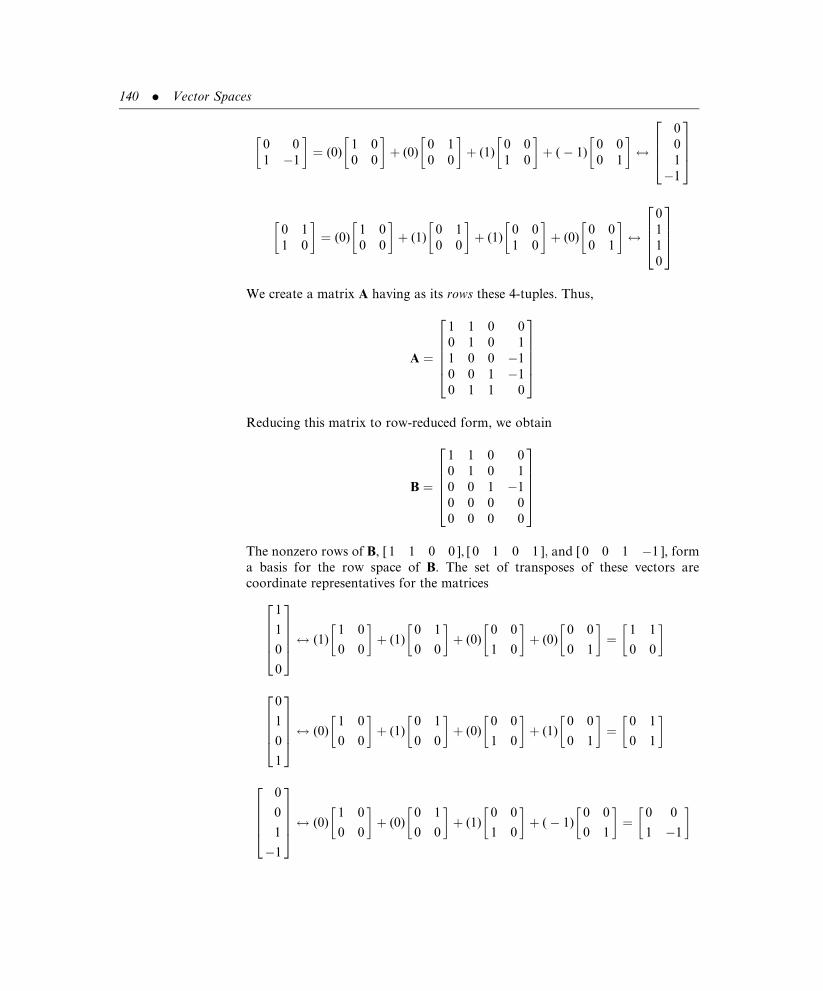
0 0
1 �1
� �¼ (0)
1 0
0 0
� �þ (0)
0 1
0 0
� �þ (1)
0 0
1 0
� �þ (� 1)
0 0
0 1
� �$
0
0
1
�1
2664
3775
0 1
1 0
� �¼ (0)
1 0
0 0
� �þ (1)
0 1
0 0
� �þ (1)
0 0
1 0
� �þ (0)
0 0
0 1
� �$
0
1
1
0
26643775
We create a matrix A having as its rows these 4-tuples. Thus,
A ¼
1 1 0 0
0 1 0 1
1 0 0 �1
0 0 1 �1
0 1 1 0
266664
377775
Reducing this matrix to row-reduced form, we obtain
B ¼
1 1 0 0
0 1 0 1
0 0 1 �1
0 0 0 0
0 0 0 0
266664
377775
The nonzero rows of B, [ 1 1 0 0 ], [ 0 1 0 1 ]; and [ 0 0 1 �1 ], form
a basis for the row space of B. The set of transposes of these vectors are
coordinate representatives for the matrices
1
1
0
0
2666437775$ (1)
1 0
0 0
� �þ (1)
0 1
0 0
� �þ (0)
0 0
1 0
� �þ (0)
0 0
0 1
� �¼
1 1
0 0
� �
0
1
0
1
2666437775$ (0)
1 0
0 0
� �þ (1)
0 1
0 0
� �þ (0)
0 0
1 0
� �þ (1)
0 0
0 1
� �¼
0 1
0 1
� �
0
0
1
�1
26664
37775$ (0)
1 0
0 0
� �þ (0)
0 1
0 0
� �þ (1)
0 0
1 0
� �þ (� 1)
0 0
0 1
� �¼
0 0
1 �1
� �
140 . Vector Spaces

These three matrices form a basis for span(R). Consequently, every matrix in the
span of R must be a linear combination of these three matrices; that is, every
matrix in span(S) must have the form
a1 1
0 0
� �þ b
0 1
0 1
� �þ g
0 0
1 �1
� �¼ a aþ b
g bþ g
� �
for any choice of the scalars a, b, and g. &
Row rank is also useful for determining if a set of n-tuples is linearly independent.
" Theorem 3. Let S be a set of k n-tuples and let A be the k� n matrix
having as its rows the n-tuples in S. S is linearly independent if and only
if the row rank of A is k, the number of elements in S. 3
Proof: Assume that the k n-tuples of S are linearly independent. Then these k
n-tuples are a basis for span(S), which means that the dimension of span(S) is k.
But the row rank of A is the dimension of the row space of A, and the row space
of A is also span(S). Because every basis for the same vector space must contain
the same number of elements (Theorem 2 of Section 2.4), it follows that the row
rank of A equals k.
Conversely, if the row rank of A equals k, then a basis for span(S) must contain k
n-tuples. The vectors in S are a spanning set for span(S), by definition. Now, either
S is linearly independent or linearly dependent. If it is linearly dependent, then one
vector must be a linear combination of vectors that precede it. Delete this vector
from S. The resulting set still spans S. Keep deleting vectors until no vector is a
linear combination of preceding vectors. At that point we have a linearly inde-
pendent set that spans S that is a basis for span(S), which contains fewer than k
vectors. This contradicts the fact that the dimension of span(S) equals k. Thus, S
cannot be linearly dependent, which implies it must linearly independent. &
Example 10 Determine whether the set
D ¼f[ 0 1 2 3 0 ], [ 1 3 �1 2 1 ],
[ 2 6 �1 �3 1 ], [ 4 0 1 0 2 ]g
is linearly independent.
Solution: We consider the matrix
A ¼
0 1 2 3 0
1 3 �1 2 1
2 6 �1 �3 1
4 0 1 0 2
2664
3775
2.5 Row Space of a Matrix . 141

which can be transformed (after the first two rows are interchanged) to the row-
reduced form
B ¼
1 3 �1 2 1
0 1 2 3 0
0 0 1 �7 �1
0 0 0 1 27=231
2664
3775
Matrix B has four nonzero rows, hence the row rank of B, as well as the row rank
of A, is four. There are four 5-tuples in D, so it follows from Theorem 3 that S is
linearly independent. &
We can extend Theorem 3 to all finite-dimensional vector spaces, not just
n-tuples. We represent every vector in a given set S by an n-tuple with respect
to a basis and then apply Theorem 3 directly to the coordinate representations.
Example 11 Determine whether the set of four polynomials in Example 8 is
linearly independent.
Solution: Coordinate representations for each of the given polynomials with
respect to the standard basis in P3 were determined in Example 8. The matrix A
in Example 8 has as its rows each coordinate representation. A can be trans-
formed into the row-reduced form of the matrix B in Example 8. It follows that
the row rank of B is two, which is also the row rank of A. This number is less
than the number of elements in S, hence S is linearly dependent. &
Problems 2.5
In Problems 1 through 21, find a basis for span(S).
(1) S ¼1
1
2
2435,
2
�1
0
24
35,
4
1
4
2435
8<:
9=;.
(2) S ¼1
1
2
2435,
2
1
0
2435,
4
1
4
2435
8<:
9=;.
(3) S ¼2
1
2
2435,
�2
�1
�2
24
35,
4
2
4
2435,
�4
�2
�4
24
35
8<:
9=;.
(4) S ¼1
0
2
2435,
�1
1
�1
24
35,
0
1
1
2435,
�1
2
0
24
35
8<:
9=;.
(5) S ¼ f[ 1 2 �1 1 ], [ 0 1 2 1 ], [ 2 3 �4 1 ], [ 2 4 �2 2 ]g.
(6) S ¼ f[ 0 1 1 1 ], [ 1 0 0 1 ], [�1 1 1 0 ], [ 1 1 0 1 ]g.
(7) S ¼ f[ 1 0 �1 1 ], [ 3 1 0 1 ], [ 1 1 2 �1 ], [ 3 2 3 �1 ],
[ 2 1 0 0 ]g.
142 . Vector Spaces

(8) S ¼ f[ 2 2 1 1 ], [ 1 �1 0 1 ], [ 0 �4 �1 1 ], [ 1 0 2 1 ],
[ 0 �1 2 2 ]g.
(9) S ¼ f[ 1 2 4 0 ], [ 2 4 8 0 ], [ 1 �1 0 1 ], [ 4 2 8 2 ],
[ 4 �1 4 3 ]g.
(10) S ¼ ft2 þ t, tþ 1, t2 þ 1, 1g.
(11) S ¼ ft2 þ tþ 1, 2t2 � 2tþ 1, t2 � 3tg.
(12) S ¼ ft, tþ 1, t� 1, 1g.
(13) S ¼ ft2 þ t, t� 1, t2 þ 1g.
(14) S ¼ ft2 þ tþ 1, tþ 1, t2g.
(15) S ¼ ft3 þ t2 � t, t3 þ 2t2 þ 1, 2t3 þ 3t2 � tþ 1, 3t3 þ 5t2 � tþ 2g.
(16) S ¼ f2t3 þ t2 þ 1, t2 þ t, 2t3 � tþ 1, tþ 1, 2t3 þ 2g.
(17) S ¼ ft3 þ 3t2, t2 þ 1, tþ 1, t3 þ 4t2 þ tþ 2, t2 þ tþ 2g.
(18) S ¼ 1 0
0 0
� �,
0 1
0 0
� �,
�1 2
0 0
� �,
1 3
0 0
� ��.
(19) S ¼ 1 1
1 0
� �,�1 1
1 0
� �,
�1 �1
1 0
� �,
1 1
�1 0
� ��.
(20) S ¼ 1 0
0 1
� �,
0 1
1 0
� �,
�1 1
1 1
� �,
1 �1
�1 1
� ��.
(21) S ¼ 1 3
1 2
� �,
1 2
1 1
� �,
�0 1
0 1
� �,
2 7
2 5
� ��.
In Problems 22 through 43, use row rank to determine whether the given sets are linearly
independent.
(22) f[ 1 0 ], [ 0 1 ]g.
(23) f[ 1 1 ], [ 1 �1 ]g.
(24) f[ 2 �4 ], [�3 6 ]g.
(25)
1
0
1
2435,
1
1
0
2435,
0
1
1
2435
8<:
9=;.
(26)
1
0
1
2435,
1
0
2
2435,
2
0
1
2435
8<:
9=;.
(27)
1
0
1
2435,
1
1
1
2435,
1
�1
1
24
35
8<:
9=;.
(28)
0
0
0
2435,
3
2
1
2435,
2
1
3
2435
8<:
9=;.
2.5 Row Space of a Matrix . 143

(29)
1
2
3
2435,
3
2
1
2435,
2
1
3
2435
8<:
9=;.
(30) f[ 1 1 0 ], [ 1 �1 0 ]g.(31) f[ 1 2 3 ], [�3 �6 �9 ]g.(32) f[ 10 20 20 ], [ 10 �10 10 ], [ 10 20 10 ]g.
(33) f[ 2 1 1 ], [ 3 �1 4 ], [ 1 3 �2 ]g.
(34)1 1
0 0
� �,
1 1
1 1
� �,
0 0
1 1
� �� �.
(35)1 1
0 0
� �,
1 0
1 1
� �,
0 0
1 1
� �� �.
(36)1 0
1 1
� �,
1 1
1 0
� �,
�1 1
0 1
� �,
0 1
1 1
� ��.
(37)1 0
1 1
� �,
1 1
1 0
� ��2 2
0 2
� �,
1 0
2 0
� ��.
(38) ft, 2g.
(39) ft3 þ t2, t3 þ t, t2 þ tg.
(40) ft3 þ t2, t3 � t2, t3 � 3t2g.
(41) ft3 þ t2, t3 � t2, t3 � t, t3 þ 1g.
(42) ft2 þ t, t2 þ t� 1, t2 þ 1, tg.
(43) ft2 þ t, t2 þ t� 2, 1g.
(44) Can a 4� 3 matrix have linearly independent rows?
(45) Prove that if the row rank of an m� n matrix is k, then k minimum fm, ng.
(46) Prove that if a matrix B is obtained from a matrix A by interchanging the positions of
any two rows of A, then both A and B have the same row space.
(47) Prove that if a matrix B is obtained from a matrix A by multiplying one row of A by
a nonzero scalar, then both A and B have the same row space.
2.6 RANK OF A MATRIX
We began this chapter noting that much of mathematical analysis is identifying
fundamental structures that appear with regularity in different situations, devel-
oping those structures in the abstract, and then applying the resulting knowledge
base back to the individual situations to further our understanding of those
situations. The fundamental structure we developed was that of a vector space.
We now use our knowledge of this structure to further our understanding of sets
of simultaneous linear equations and matrix inversion.
144 . Vector Spaces

In the last section we defined the row space of a matrix A to be the subspace
spanned by the rows of A, considered as row matrices. We now define the column
space of a matrix A to be the subspace spanned by the columns of A, considered
as column matrices. The dimension of the column space is called the column
rank of A.
Example 1 The matrix A ¼ 1 2 3
4 5 6
� �has three columns, all belonging to R2.
The column space of A consists of all linear combinations of the columns of A;
that is, if we set
T ¼ 1
4
� �,
2
5
� �,
3
6
� �� �
then the column space of A is span(T). The dimension of span(T) is the column
rank of A. &
The row space of a p� n matrix A is a subspace of Rn while its column space is a
subspace of Rp, and these are very different vector spaces when p and n are
unequal. Surprisingly, both have the same dimension. The proof of this state-
ment is a bit lengthy, so we separate it into two parts.
" Lemma 1. The column rank of a matrix is less than or equal to its row
rank. 3
Proof: Let A1, A2, . . . , Ap be the rows, considered as row matrices, of a p� n
matrix A ¼ [aij ]. Then
Ai ¼ [ ai1 ai2 . . . ain ]; (i ¼ 1, 2, . . . , p)
Let k denote the row rank of A. Thus, k is the dimension of the subspace spanned
by the rows of A, and this subspace has a basis containing exactly k vectors.
Designate one such basis as the set B ¼ fu1, u2, . . . , ukg. Each vector in the basis
is an n-tuple of the form
ui ¼ [ ui1 ui2 � � � uin ]; (i ¼ 1, 2, . . . , k)
Since B is a basis, every vector in the subspace spanned by the rows of A can be
written as a linear combination of the vectors in B, including the rows of A
themselves. Thus,
A1 ¼ d11u1 þ d12u2 þ � � � þ d1kuk
A2 ¼ d21u1 þ d22u2 þ � � � þ d2kuk
..
.
Ap ¼ dp1u1 þ dp2u2 þ � � � þ dpkuk
The column space of
a matrix is the
subspace spanned
by the columns of
the matrix; the
dimension of the
column space is the
column rank.
2.6 Rank of a Matrix . 145

for some set of uniquely determined scalars dij (i ¼ 1, 2, . . . ; j ¼ 1, 2, . . . , k).
In each of the preceding individual equalities, both the left and right sides are
n-tuples. If we consider just the jth component of each n-tuple ( j ¼ 1, 2, . . . , n),
first the jth component of A1, then the jth component of A2, sequentially through
the jth component of Ap, we obtain the equalities
a1j ¼ d11u1j þ d12u2j þ � � � þ d1kukj
a2j ¼ d21u1j þ d22u2j þ � � � þ d2kukj
..
.
apj ¼ dp1u1j þ dp2u2j þ � � � þ dpkukj
which can be rewritten as the vector equation
a1j
a2j
..
.
apj
26664
37775 ¼ u1j
d11
d21
..
.
dp1
26664
37775þ u2j
d12
d22
..
.
dp2
26664
37775þ � � � þ ukj
d1k
d2k
..
.
dpk
26664
37775
Thus, the jth column of A can be expressed as a linear combination of k vectors.
Since this is true for each j, it follows that each column of A can be expressed as a
linear combination of the same k vectors, which implies that the dimension of the
column space of A is at most k. That is, the column rank of A k ¼ the row
rank of A.
" Theorem 1. The row rank of a matrix equals its column rank. 3
Proof: For any matrix A, we may apply Lemma 1 to its transpose and conclude
that the column rank of AT is less than or equal to its row rank. But since the
columns of AT are the rows of A and vice versa, it follows that the row rank of A
is less than or equal to its column rank. Combining this result with Lemma 1, we
have Theorem 1. &
Since the row rank and column rank of a matrix A are equal, we refer to them
both simply as the rank of A, denoted as r(A).
With the concepts of vector space, basis, and rank in hand, we can give explicit
criteria for determining when solutions to sets of simultaneous linear equations
exist. In other words, we can develop a theory of solutions to complement our
work in Chapter 1.
The rank of a
matrix A, denoted
as r(A), is the row
rank of A, which is
also the column
rank of A.
146 . Vector Spaces

A system of m simultaneous linear equations in n unknowns has the form
a11x1 þ a12x2 þ � � � þ a1nxn ¼ b1
a21x1 þ a22x2 þ � � � þ a2nxn ¼ b2
..
.
am1x1 þ am2x2 þ � � � þ amnxn ¼ bm
(2:20)
or the matrix form
Ax ¼ b (2:21)
If we denote the columns of A by the m-dimensional column matrices
A1 ¼
a11
a21
..
.
am1
26664
37775, A2 ¼
a12
a22
..
.
am2
26664
37775, � � � , An ¼
a1n
a2n
..
.
amn
26664
37775
then we can rewrite (2.20) in the vector form
x1A1 þ x2A2 þ � � � þ xnAn ¼ b (2:22)
Example 2 The system of equations
x� 2yþ 3z ¼ 7
4xþ 5y� 6z ¼ 8
has the vector form
x1
4
� �þ y
�2
5
� �þ z
3
�6
� �¼ 7
8
� �&
Solving (2.20) or (2.21) is equivalent to finding scalars x12, . . . , xn that satisfy
(2.22). If such scalars exist, then the vector b is a linear combination of the
vectors A1, A2, . . . , An. That is, b is in the span of fA1, A2, . . . , Ang or, equiva-
lently, in the column space of A. Consequently, adjoining b to the set of vectors
defined by the columns of A will not change the column rank of A. Therefore, the
column rank of A must equal the column rank of [Ajb]. On the other hand, if no
scalars x1, x2, . . . , xn satisfy (2.22), then b is not a linear combination of
A1, A2, . . . , An. That is, b is not in the span of fA1, A2, . . . , Ang, in which case,
the column rank of [Ajb] must be greater by 1 than the column rank of A. Since
column rank equals row rank equals rank, we have proven Theorem 2.
2.6 Rank of a Matrix . 147

" Theorem 2. The system Ax ¼ b is consistent if and only if
r(A) ¼ r[Ajb]. 3
Example 3 Determine whether the following system of equations is consistent:
xþ y� z ¼ 1
xþ y� z ¼ 0
Solution:
A ¼ 1 1 �1
1 1 �1
� �, b ¼ 1
0
� �, [Ajb] ¼ 1 1 �1
1 1 �1
10� �
[Ajb] is transformed to row-reduced form
1 1 �1
1 1 �1
10� �
!1 1 �1
0 0 0
1
�1
� � by adding to the
second row
� 1 times the first row
!1 1 �1
0 0 0
11� � by multiplying
the second row
by � 1
(2:23)
This matrix has two nonzero rows, hence r[Ajb] ¼ 2. If we delete the last column
from the matrix in (2.23), we have A in the row-reduced form
1 1 �1
0 0 0
� �
This matrix has one nonzero row, so r(A) ¼ 1. Since r(A) 6¼ r[Ajb], it follows
from Theorem 2 that the given set of equations has no solution and is not
consistent. &
Example 4 Determine whether the following system of equations is consistent:
xþ yþ w ¼ 3
2xþ 2yþ 2w ¼ 6
�x� y� w ¼ �3
Solution:
A ¼1 1 1
2 2 2
�1 �1 �1
24
35, b ¼
3
6
�3
24
35, [Ajb] ¼
1 1 1
2 2 2
�1 �1 �1
3
6
�3
24
35
148 . Vector Spaces
By transforming both A and [Ajb] to row-reduced form, we can show that
r(A) ¼ r[Ajb] ¼ 1. Therefore, the original system is consistent. &
Once a system is determined to be consistent, the following theorem specifies the
number of solutions.
" Theorem 3. If the system Ax ¼ b is consistent and if r(A) ¼ k, then
solutions to the system are expressible in terms of n� k arbitrary
unknowns, where n denotes the total number of unknowns in the
system. 3
Proof: To determine the rank of the augmented matrix [Ajb], reduce the
augmented matrix to row-reduced form and count the number of nonzero
rows. With Gaussian elimination, we can solve the resulting row-reduced matrix
for the variables associated with the first nonzero entry in each nonzero row.
Thus, each nonzero row defines one variable and all other variables remain
arbitrary. &
Example 5 Determine the number of solutions to the system described in
Example 4.
Solution: The system has three unknowns, x, y, and w, hence n ¼ 3. Here
r(A) ¼ r[Ajb] ¼ 1, so k ¼ 1. The solutions are expressible in terms of 3� 1 ¼ 2
arbitrary unknowns. Using Gaussian elimination, we find the solution as
x ¼ 3� y� w with both y and w arbitrary. &
Example 6 Determine the number of solutions to the system
2x� 3yþ z ¼ �1
x� yþ 2z ¼ 2
2xþ y� 3z ¼ 3
Solution:
A ¼2 �3 1
1 �1 2
2 1 �3
24
35, b ¼
�1
2
3
24
35, [Ajb] ¼
2 �3 1
1 �1 2
2 1 �3
�1
2
3
24
35
By transforming both A and [Ajb] to row-reduced form, we can show that
r(A) ¼ r[Ajb] ¼ 3; hence, the given system is consistent. In this case, n ¼ 3
(three variables) and (rank) k ¼ 3; the solutions are expressible in terms of
3� 3 ¼ 0 arbitrary unknowns. Thus, the solution is unique (none of the un-
knowns is arbitrary). Using Gaussian elimination, we find the solution as
x ¼ y ¼ 2, z ¼ 1. &
2.6 Rank of a Matrix . 149

A homogeneous system of simultaneous linear equations has the form
a11x1 þ a12x2 þ � � � þ a1nxn ¼ 0
a21x1 þ a22x2 þ � � � þ a2nxn ¼ 0
..
.
am1x1 þ am2x2 þ � � � þ amnxn ¼ 0
(2:24)
or the matrix form
Ax ¼ 0 (2:25)
Since (2.25) is a special case of (2.21) with b ¼ 0, Theorems 2 and 3 remain valid.
Because of the simplified structure of a homogeneous system, however, we can
draw conclusions about it that are not valid for nonhomogeneous systems. In
particular, a homogeneous system is consistent, because the trivial solution x ¼ 0
is always a solution to Ax ¼ 0. Furthermore, if the rank of A equals the number
of unknowns, then the solution is unique and the trivial solution is the only
solution. On the other hand, it follows from Theorem 3 that if the rank of A is
less than the number of unknowns, then the solution will be in terms of arbitrary
unknowns. Since these arbitrary unknowns can be assigned nonzero values,
nontrivial solutions exist. Thus, we have Theorem 4.
" Theorem 4. A homogeneous system of equations Ax ¼ 0 in n unknowns
will admit nontrivial solutions if and only if r(A) 6¼ n. 3
The concept of rank also provides the tools to prove two results we simply stated
in the previous chapter. We can now determine a criterion for the existence of an
inverse and also show that, for square matrices, the equality AB ¼ I implies the
equality BA ¼ I. For convenience, we separate the analysis into segments.
" Lemma 2. Let A and B be n� n matrices. If AB ¼ I, then the system of
equations Ax ¼ y has a solution for every choice of the vector y. 3
Proof: Once y is specified, set x ¼ By. Then
Ax ¼ A(By) ¼ (AB)y ¼ Iy ¼ y
hence x ¼ By is a solution of Ax ¼ y. &
" Lemma 3. If A and B are n� n matrices with AB ¼ I, then the rows
of A, considered as n-dimensional row matrices, are linearly
independent. 3
A homogeneous
system of equations
is always consistent,
and one solution is
always the trivial
solution.
150 . Vector Spaces

Proof: Designate the rows of A by A1, A2, . . . , An, respectively, and the columns
of I as the vectors e1, e2, . . . , en, respectively. It follows from Lemma 2 that the
set of equations Ax ¼ ej ( j ¼ 1, 2, . . . , n) has a solution for each j. Denote these
solutions by x1, x2, . . . , xn, respectively. Therefore,
Axj ¼ ej (2:26)
Since ej is an n-dimensional column matrix having a unity element in row j and
zeros elsewhere, it follows from (2.26) that, for i ¼ 1, 2, . . . , n,
ith component of Axj ¼1 when i ¼ j
0 when i 6¼ j
�
This equation can be simplified if we make use of the Kronecker delta dij
defined as
dij ¼1 when i ¼ j
0 when i 6¼ j
�(2:27)
Thus, (2.26) may be written as
ith component of Axj ¼ dij
or, more simply, as
Aixj ¼ dij (2:28)
Now consider the vector equation
Xn
i¼1
ciAi ¼ 0 (2:29)
We want to show that each constant ci (i ¼ 1, 2, . . . , n) must be 0. Multiplying
both sides of (2.29) on the right by the vector xj , and using Eqs. (2.27) and (2.28),
we have
0 ¼ 0xj ¼Xn
i¼1
ciAi
!xj ¼
Xn
i¼1
(ciAi)xj ¼Xn
i¼1
ci(Aixj) ¼Xn
i¼1
cidij ¼ cj
Thus, for each xj ( j ¼ 1, 2, . . . , n) we have cj ¼ 0, which implies that
c1 ¼ c2 ¼ � � � ¼ cn ¼ 0 and that the rows of A, namely, A1, A2, . . . , An, are lin-
early independent. &
It follows directly from Lemma 3 and the definition of an inverse that if an n� n
matrix A has an inverse, then A must have rank n. This in turn implies that if A
2.6 Rank of a Matrix . 151

does not have rank n, then A does not have an inverse. We also want the
converse: that is, if A has rank n, then A has an inverse.
" Lemma 4. If an n� n matrix A has rank n, then there exists a square
matrix C such that CA ¼ I. 3
Proof: If an n� n matrix A has rank n, then its row-reduced form is an upper
triangular matrix with all elements on the main diagonal equal to 1. Using these
diagonal elements as pivots, we can use elementary row operations to further
transform A to an identity matrix. Corresponding to each elementary row
operation is an elementary matrix. Therefore, if A has rank n, then there is
a sequence of elementary matrices E1, E2, . . . , Ek�1, Ek such that
EkEk�1 . . . E2E1A ¼ I
Setting
C ¼ EkEk�1 . . . E2E1 (2:30)
we have
CA ¼ I & (2:31)
" Lemma 5. If A and B are n� n matrices such that AB ¼ I, then
BA ¼ I. 3
Proof: If AB ¼ I, then it follows from Lemma 3 that A has rank n. It then
follows from Lemma 4 that there exists a matrix C such that CA ¼ I. Conse-
quently,
C ¼ CI ¼ C(AB) ¼ (CA)B ¼ IB ¼ B
so the equality CA ¼ I implies that BA ¼ I. &
If we replace A by C and B by A in Lemma 5, we have that, if C and A are n� n
matrices such that CA ¼ I, then it is also true that
AC ¼ I (2:32)
Therefore, if A is an n� n matrix with rank n, then (2.31) holds, whereupon
(2.32) also holds. Together (2.31) and (2.32) imply that C is the inverse of A.
Thus, we have proven Theorem 5.
152 . Vector Spaces

" Theorem 5. An n� n matrix A has an inverse if and only if A has
rank n. 3
In addition, we also have Theorem 6.
" Theorem 6. A square matrix has an inverse if and only if it can be
transformed by elementary row operations to an upper triangular matrix
with all elements on the main diagonal equal to 1. 3
Proof: An n� n matrix A has an inverse if and only if it has rank n (Theorem 5).
It has rank n if and only if it can be transformed by elementary row operations
into a row-reduced matrix B having rank n (Theorem 2 of Section 2.5). B has
rank n if and only if it contains n nonzero rows (Theorem 1 of Section 2.5).
A row-reduced, n� n matrix B has n nonzero rows if and only if it is upper
triangular with just ones on its main diagonal.
Problems 2.6
In Problems 1 through 7, find the ranks of the given matrices.
(1)1 2 0
3 1 �5
� �. (2)
2 8 �6
�1 �4 3
� �.
(3)
4 1
2 3
2 2
24
35. (4)
4 8
6 12
9 18
24
35.
(5)
1 4 �2
2 8 �4
�1 �4 2
24
35. (6)
1 2 4 2
1 1 3 2
1 4 6 2
24
35.
(7)
1 7 0
0 1 1
1 1 0
24
35.
(8) What is the largest possible value for the rank of a 2� 5 matrix?
(9) What is the largest possible value for the rank of a 4� 3 matrix?
(10) What is the largest possible value for the rank of a 4� 6 matrix?
(11) Show that the rows of a 5� 3 matrix are linearly dependent.
(12) Show that the columns of a 2� 4 matrix are linearly dependent.
(13) What is the rank of a zero matrix?
(14) Use the concept of rank to determine whether [ 3 7 � can be written as a linear
combination of the following sets of vectors.
(a) f[ 1 2 �, [ 4 8 �g, (b) f[ 1 2 �, [ 3 2 �g.
2.6 Rank of a Matrix . 153

(15) Use the concept of rank to determine whether [ 2 3 � can be written as a linear
combination of the following sets of vectors.
(a) f[ 10 15 �, [ 4 6 �g, (b) f[ 1 1 �, [ 1 �1 �g,
(c) f[ 2 �4 �, [�3 6 �g.
(16) Use the concept of rank to determine whether [ 1 1 1 �T can be written as a linear
combination of the following sets of vectors.
(a)
1
0
1
2435,
1
1
0
2435,
0
1
1
2435
8<:
9=;, (b)
1
0
1
2435,
1
0
2
2435,
2
0
1
2435
8<:
9=;,
(c)
1
0
1
2435,
1
1
1
2435,
1
�1
1
24
35
8<:
9=;.
In Problems 17 through 25, discuss the solutions of the given systems of equations in
terms of consistency and number of solutions. Check your answers by solving the systems
wherever possible.
(17) x� 2y ¼ 0
xþ y ¼ 1
2x� y ¼ 1
(18) xþ y ¼ 0
2x� 2y ¼ 1
x� y ¼ 0
(19) xþ yþ z ¼ 1
x� yþ z ¼ 2
3xþ yþ 3z ¼ 4
(20) xþ 3yþ 2z� w ¼ 2
2x� yþ zþ w ¼ 3
(21) 2x� yþ z ¼ 0
xþ 2y� z ¼ 4
xþ yþ z ¼ 1
(22) 2xþ 3y ¼ 0
x� 4y ¼ 0
(23) x� yþ 2z ¼ 0
2xþ 3y� z ¼ 0
�2xþ 7y� 7z ¼ 0
(24) x� yþ 2z ¼ 0
2x� 3yþ 5z ¼ 0
�2xþ 7y� 9z ¼ 0
(25) x� 2yþ 3zþ 3w ¼ 0
y� 2zþ 2w ¼ 0
xþ y� 3zþ 9w ¼ 0
154 . Vector Spaces

Chapter 2 Review
Important Terms
Important Concepts
Section 2.1 " The zero vector in a vector space is unique.
" The additive inverse of any vector v in a vector space is unique and is equal to�1 � v.
Section 2.2 " A nonempty subset S of a vector space V is a subspace of V if and only if S is
closed under addition and scalar multiplication.
" If a subset of a vector space does not include the zero vector, then that subset
cannot be a subspace.
" Lines through the origin and planes that contain the origin are subspaces of R3.
" The span of a set of vectors S in a vector space V is the smallest subspace of V
that contains S.
Section 2.3 " A set of vectors is linearly dependent if and only if one of the vectors is a linear
combination of the vectors that precede it.
" Twovectors are linearly dependent in R2 or R3 if and only if they lie on the same line.
" A set of three vectors in R3 is linearly dependent if and only if all three vectors lie
on the same line or all lie on the same plane.
Section 2.4 " dim(Rn) ¼ n; dim(Pn) ¼ nþ 1; dim(Mp�n) ¼ pn:
" Every basis for a finite-dimensional vector space contains the same number of
vectors.
" In an n-dimensional vector space, every set of nþ 1 or more vectors is linearly
dependent.
additive inverse (p. 86)
basis (p. 120)
column rank (p. 145)
column space(p. 145)
coordinates (p. 128)
dimension (p. 124)
finite-dimensional vector space
(p. 122)
linear combinations (p. 106)
linearly dependent vectors (p. 110)
linearly independent vectors
(p. 110)
Mp�n (p. 89)
Pn (p. 92)
Rn (p. 89)
rank (p. 144)
row rank (p. 134)
row space (p. 134)
span of vectors (p. 106)
spanning set (p. 119)
subspace (p. 99)
vector (p. 86)
vector space (p. 86)
zero vector (p. 93)
Chapter 2 Review . 155

" A spanning set of vectors for a finite-dimensional vector space V can be reduced
to a basis for V; a linearly independent set of vectors in V can be expanded into
a basis.
Section 2.5 " If matrix B is obtained from matrix A by an elementary row operation, then the
row space of A is the same as the row space of B.
" To find the row rank of a matrix, use elementary row operations to transform the
matrix to row-reduced form and then count the number of nonzero rows. The
nonzero rows are a basis for the row space of the original matrix.
Section 2.6 " The row rank of a matrix equals its column rank.
" The system of equation Ax ¼ b is consistent if and only if the rank of A equals
the rank of the augmented matrix [Ajb�.
" If the system Ax ¼ b is consistent and if r(A) ¼ k, then the solutions to the system
are expressible in terms of n� k arbitrary unknowns, where n denotes the total
number of unknowns in the system.
" A homogeneous system of equations is always consistent, and one solution is
always the trivial solution.
" An n� n matrix A has an inverse if and only if A has rank n.
" A square matrix has an inverse if and only if it can be transformed by elementary
row operations to an upper triangular matrix with all unity elements on its main
diagonal.
156 . Vector Spaces

Chapter 3
Linear Transformations
3.1 FUNCTIONS
Relationships between items are at the heart of everyday interactions, and if
mathematics is to successfully model or explain such interactions, then math-
ematics must account for relationships. In commerce, there are relationships
between labor and production, between production and profit, and between
profit and investment. In physics, there are relationships between force and
acceleration, and between mass and energy. In sociology, there is a relationship
between control and evasions. We need, therefore, mathematical structures to
represent relationships. One such structure is a function.
A function is a rule of correspondence between two sets, generally called the
domain and range, that assigns to each element in the domain exactly one element
(but not necessarily a different one) in the range.
Example 1 The rules of correspondence described by the arrows in Figures 3.1
and 3.2 between the domain {A,B,C} and the range {1,2,3,4,5} are functions.
In both cases, each element in the domain is assigned exactly one element in the
range. In Figure 3.1, A is assigned 1, B is assigned 3, and C is assigned 5.
Although some elements in the range are not paired with elements in the
domain, this is of no consequence. A function must pair every element in
A function is a rule
of correspondence
between two sets,
a domain and range,
that assigns to each
element in the
domain exactly one
element (but not
necessarily a
different one) in
the range.
Figure 3.1
A 2
1
3
4
5
B
C
157

the domain with an element in the range, but not vice versa. In Figure 3.2, each
element in the domain is assigned the same element in the range, namely, 2. This
too is of no consequence. A function must pair every element in the domain with
an element in the range, but not necessarily with a different element. &
Example 2 The rule of correspondence described by the arrows in Figure 3.3
between the domain and range, which are both the set of words {dog, cat, bird}, is
not a function. The word cat, in the domain, is not matched with any element in
the range. A function must match every element in the domain with an element
in the range. &
The image of a function consists of those elements in the range that are matched
with elements in the domain. An element y in the range is in the image only if
there is an element x in the domain such that x is assigned the value y by the rule
of correspondence. In Figure 3.1, the image is the set {1, 3, 5} because 1, 3, and 5
are the only elements in the range actually assigned to elements in the domain.
In Figure 3.2, the image is the set {2} because the number 2 is the only number in
the range matched with elements in the domain.
The domain and range of a function can be any type of set, ranging from sets of
letters to sets of colors to sets of animals, while the rule of correspondence can be
specified by arrows, tables, graphs, formulas, or words. If we restrict ourselves to
sets of real numbers and rules of correspondence given by equations, then we
have the functions studied most often in algebra and calculus.
Figure 3.2
A 2
1
3
4
5
B
C
Figure 3.3dog dog
bird bird
cat cat
The image of a
function is the set of
all elements in the
range that are
matched with
elements in the
domain by the rule
of correspondence.
158 . Linear Transformations

Whenever we have two sets of numbers and a function f relating the arbitrary
element x in the domain to the element y in the range through an equation, we
say that y is a function of x and write y ¼ f (x). Letters other than x and y may be
equally appropriate. The equation R ¼ f (N) is shorthand notation for the state-
ment that we have a function consisting of two sets of numbers and an equation,
where N and R denote elements in the domain and range, respectively. If the
domain is not specified, it is assumed to be all real numbers for which the rule of
correspondence makes sense; if the range is not specified, it is taken to be the set
of all real numbers.
If we have a rule of correspondence defined by the formula f (x), then we find the
element in the range associated with a particular value of x by replacing x with
that particular value in the formula. Thus, f (2) is the effect of applying the rule of
correspondence to the domain element 2, while f (5) is the effect of applying the
rule of correspondence to the domain element 5.
Example 3 Find f (2), f (5), and f (� 5) for f (x) ¼ 1=x2.
Solution: The domain and range are not specified, so they assume their default
values. The formula 1=x2 is computable for all real numbers except 0, so this
becomes the domain. The range is the set of all real numbers. The image is all
positive real numbers because those are the only numbers actually matched to
elements in the domain by the formula. Now
f (2) ¼ 1=(2)2 ¼ 1=4 ¼ 0:25
f (5) ¼ 1=(5)2 ¼ 1=25 ¼ 0:04
f (� 5) ¼ 1=(� 5)2 ¼ 1=25 ¼ 0:04 &
Problems 3.1
In Problems 1 through 16, the rules of correspondence are described by arrows. Determine
whether the given relationships are functions and, for those that are, identify their images.
(1)A
1 2 3 4 5
B C D E(2)
A B C D E
A B C D E
3.1 Functions . 159
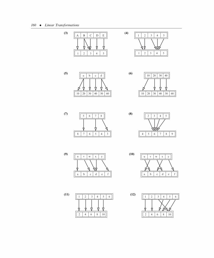
(3)A
1 2 3 4 5
B C D E(4)
1
1 2 3 4 5
2 3 4 5
(5)a
10 20 30 40 50 60
b c d(6)
10
10 20 30 40 50 60
20 30 40
(7)5
8 7 6 5 4 3
6 7 8(8)
2
4 5 6 7 8 9
3 4 5
(9)yxwvu
a b c d e f
(10)yxwvu
a b c d e f
(11)
108642
1 2 3 4 5 6(12)
108642
1 2 3 4 5 6
160 . Linear Transformations

(13)1
red blue green yellow
2 3 4 5
(14)1
blue green yellow
2 3 4 5
(15)−1
10.3 18.6 22.7
−2 −3 −4 −5
In Problems 16 through 18, determine whether the given tables represent functions where
the rule of correspondence is to assign to each element in the top row the element directly
below it in the bottom row.
In Problems 19 through 22, determine whether the specified correspondences constitute
functions.
(19) The correspondence between people and their weights.
(20) The correspondence between people and their social security numbers.
(21) The correspondence between cars and the colors they are painted.
(22) The correspondence between stocks listed on the New York Stock Exchange and
their closing prices on a given day.
(16) x 1 2 3 4 5
y 10 18 23 18 10
(17) x 1 2 3 4 5
y 10 10 20 20 20
(18) x 1 2 3 4 5
y 10 18 23 29 34
3.1 Functions . 161

In Problems 23 through 29, determine whether a domain exists on the horizontal axis so
that the given graphs represent functions. The rule of correspondence assigns to each
x value in the domain all y values on the vertical axis (the range) for which the points (x, y)
lie on the graph.
(23)
2
1
1 2 3 4x
y
0−1
(24) 5
3
4 5x
y
3
21
1−1−2−3−4
−4
−5
(25)
5
5x
y
−5
−5
(26)
4
x
y
5−5
−4
(27)
4
x
y
5−5
−4
(28)
(0,3)
0x
y
(4,0)(−4,0)
(0,−4)
(29)
(0,3)
0x
y
(4,0)(−4,0)
(0,−4)
(30) Determine whether the following equations represent functions on the specified
domains:
(a) y ¼ þffiffiffixp
for �1 < x <1.
(b) y ¼ þffiffiffixp
for 0 < x <1.
(c) y ¼ �ffiffiffixp
for 0 < x <1.
(d) y ¼ffiffiffix3p for�1 < x <1.
162 . Linear Transformations

(31) Given the function y ¼ f (x) ¼ x2 � 3xþ 2 defined on all real numbers, find
(a) f (0), (b) f (1), (c) f (� 1), (d) f (2x).
(32) Given the function y ¼ f (x) ¼ 2x2 � x defined on all real numbers, find
(a) f (1), (b) f (� 1), (c) f (2x), (d) f (aþ b).
(33) Given the function y ¼ f (x) ¼ x3 � 1 defined on all real numbers, find
(a) f (� 2), (b) f (0), (c) f (2z), (d) f (aþ b).
(34) A function is onto if its image equals its range. Determine whether either of the
functions defined in Example 1 are onto.
(35) Determine which of the functions defined in Problems 1 through 15 are onto.
(36) A function is one to one if the equality f (x) ¼ f (z) implies that x ¼ z; that is, if each
element in the image is matched with one and only one element in the domain.
Determine whether either of the functions defined in Example 1 are one to one.
(37) Determine which of the functions defined in Problems 1 through 15 are one to one.
3.2 LINEAR TRANSFORMATIONS
Two frequently used synonyms for the word function are mapping and trans-
formation. In high-school algebra and calculus, the domain and range are
restricted to subsets of the real numbers and the word function is used almost
exclusively. In linear algebra, the domain and range are vector spaces and the
word transformation is preferred.
A transformation T is a rule of correspondence between two vector spaces,
a domain V and a range W, that assigns to each element in V exactly one element
(but not necessarily a different one) in W. Such a transformation is denoted by
the shorthand notation T: V!W. We write w ¼ T(v) whenever the vector w in
W is matched with the vector v in V by the rule of correspondence associated
with T. We will, on occasion, discard the parentheses and write w ¼ Tv when
there is no confusion as to what this notation signifies.
The image of T is the set of all vectors in W that are matched with vectors in V
under the rule of correspondence. Thus, w is in the image of T if and only if there
exists a vector v in V such that w ¼ T(v).
A transformation T: V!W is linear if for any two scalars, a and b, and any two
vectors, u and v, in V the following equality holds:
T(auþ bv) ¼ aT(u)þ bT(v) (3:1)
For the special case a ¼ b ¼ 1, (3.1) reduces to
T(uþ v) ¼ T(u)þ T(v) (3:2)
A transformation is
a function with
vector spaces for its
domain and range.
3.2 Linear Transformations . 163

while for the special case b ¼ 0, (3.1) becomes
T(au) ¼ aT(u) (3:3)
Verifying (3.1) is equivalent to verifying (3.2) and (3.3) separately (see
Problem 47).
The left side of (3.1) is the mapping of the linear combination auþ bv from the
vector space V into the vector space W. If T is linear, then the result of mapping
auþ bv into W is the same as separately mapping u and v into W, designated as
T(u) and T(v), and then forming the identical linear combination with T(u) and
T(v) in W as was formed in V with u and v; namely, a times the first vector plus
b times the second vector. Linear combinations are fundamental to vector spaces
because they involve the only operations, addition and scalar multiplication,
guaranteed to exist in a vector space. Of all possible transformations, linear
transformations are those special ones that preserve linear combinations.
Example 1 Determine whether the transformation T: V! V defined by
T(v) ¼ kv for all vectors v in V and any scalar k is linear.
Solution: In this example, V ¼W; that is, both the domain and the range are
the same vector space. For any two vectors u and v in V, we have
T(auþ bv) ¼ k(auþ bv) ¼ a(ku)þ b(kv) ¼ aT(u)þ bT(v)
Thus, (3.1) is valid, and the transformation is linear. &
The linear transformation in Example 1 is called a dilation. In R2, a dilation
reduces to a scalar multiple of a 2-tuple, having the geometrical effect of elong-
ating v by a factor of jkj when jkj > 1 or contracting v by a factor of jkj when
jkj < 1 followed by a rotation of 1808 when k is negative and no rotation when k
is positive. These dilations are illustrated in Figure 3.4. When V ¼ R2 and
k ¼ �1, the transformation T is sometimes called a rotation through the origin.
It is illustrated in Figure 3.5.
Figure 3.4
x
y
3v
v
uu
u1−
12
2
−2v
A transformation is
linear if it preserves
linear combinations.
164 . Linear Transformations

Example 2 Determine whether the transformation T: V!W defined by
T(v) ¼ 0 for all vectors v in V is linear.
Solution: For any two scalars a and b and for any two vectors u and v in V, we
have
T(auþ bv) ¼ 0 ¼ 0þ 0 ¼ a0þ b0 ¼ aT(u)þ bT(v)
Thus, (3.1) is valid, and T is linear. Transformations of this type are called zero
transformations because they map all vectors in the domain into the zero vector
in W. &
Example 3 Determine whether the transformation L is linear if L: P3 ! P2 is
defined by
L(a3t3 þ a2t
2 þ a1tþ a0) ¼ 3a3t2 þ 2a2tþ a1
where ai (i ¼ 0, 1, 2, 3) denotes a real number.
Solution: A transformation is linear if it satisfies (3.1) or, equivalently, both
(3.2) and (3.3). For practice, we try to validate (3.2) and (3.3). Setting
u ¼ a3t3 þ a2t
2 þ a1tþ a0 and v ¼ b3t3 þ b2t
2 þ b1tþ b0
we have L(u) ¼ 3a3t2 þ 2a2tþ a1, L(v) ¼ 3b3t
2 þ 2b2tþ b1, and
Figure 3.5
v
w
xz
y
u
−u
−v
−z
−w
3.2 Linear Transformations . 165
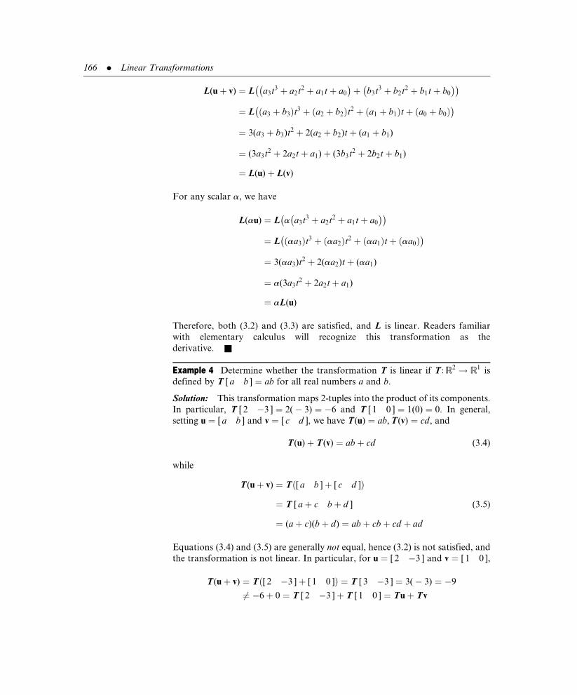
L(uþ v) ¼ L a3t3 þ a2t
2 þ a1tþ a0
� �þ b3t
3 þ b2t2 þ b1tþ b0
� �� �¼ L a3 þ b3ð Þt3 þ a2 þ b2ð Þt2 þ a1 þ b1ð Þtþ a0 þ b0ð Þ
� �¼ 3(a3 þ b3)t
2 þ 2(a2 þ b2)tþ (a1 þ b1)
¼ (3a3t2 þ 2a2tþ a1)þ (3b3t
2 þ 2b2tþ b1)
¼ L(u)þ L(v)
For any scalar a, we have
L(au) ¼ L a a3t3 þ a2t
2 þ a1tþ a0
� �� �¼ L aa3ð Þt3 þ aa2ð Þt2 þ aa1ð Þtþ aa0ð Þ
� �¼ 3(aa3)t
2 þ 2(aa2)tþ (aa1)
¼ a(3a3t2 þ 2a2tþ a1)
¼ aL(u)
Therefore, both (3.2) and (3.3) are satisfied, and L is linear. Readers familiar
with elementary calculus will recognize this transformation as the
derivative. &
Example 4 Determine whether the transformation T is linear if T: R2 ! R1 is
defined by T [ a b ] ¼ ab for all real numbers a and b.
Solution: This transformation maps 2-tuples into the product of its components.
In particular, T [ 2 �3 ] ¼ 2(� 3) ¼ �6 and T [ 1 0 ] ¼ 1(0) ¼ 0. In general,
setting u ¼ [ a b ] and v ¼ [ c d ], we have T(u) ¼ ab, T(v) ¼ cd, and
T(u)þ T(v) ¼ abþ cd (3:4)
while
T(uþ v) ¼ T [ a b ]þ [ c d ]ð Þ
¼ T [ aþ c bþ d ]
¼ (aþ c)(bþ d) ¼ abþ cbþ cd þ ad
(3:5)
Equations (3.4) and (3.5) are generally not equal, hence (3.2) is not satisfied, and
the transformation is not linear. In particular, for u ¼ [ 2 �3 ] and v ¼ [ 1 0 ],
T(uþ v) ¼ T [ 2 �3 ]þ [ 1 0 ]ð Þ ¼ T [ 3 �3 ] ¼ 3(� 3) ¼ �9
6¼ �6þ 0 ¼ T [ 2 �3 ]þ T [ 1 0 ] ¼ Tuþ Tv
166 . Linear Transformations

We can also show that (3.3) does not hold, but this is redundant. If either (3.2) or
(3.3) is violated, the transformation is not linear. &
Example 5 Determine whether the transformation T is linear if T: R2 ! R2 is
defined by T [ a b ] ¼ [ a �b ] for all real numbers a and b.
Solution: This transformation maps 2-tuples into 2-tuples by changing the sign
of the second component. Here, T [ 2 3 ] ¼ [ 2 �3 ], T [ 0 �5 ] ¼ [ 0 5 ], and
T [�1 0 ] ¼ [�1 0 ]. In general, setting u ¼ [ a b ] and v ¼ [ c d ], we have
T(u) ¼ [ a �b ], T(v) ¼ [ c �d ], and
T(uþ v) ¼ T [ a b ]þ [ c d ]ð Þ
¼ T [ aþ c bþ d ]
¼ [ aþ c �(bþ d) ]
¼ [ aþ c �b� d ]
¼ [ a �b ]þ [ c �d ]
¼ T(u)þ T(v)
For any scalar a, we have
T(au) ¼ T a[ a b ]ð Þ ¼ T [ aa ab ] ¼ [ aa �ab ] ¼ a[ a �b ] ¼ aT(u)
Thus, (3.2) and (3.3) are satisfied, and the transformation is linear. &
The linear transformation T defined in Example 5 is called a reflection across
the x-axis. For vectors graphed on an x-y coordinate system, the transformation
Figure 3.6
(4, 2)
4
5
3
2
1u
v
x
y
1 2 3 4 5
−2
−1−1−2−3
−3
−4
(4, −2)
(−1,−4)
(−1, 4)
T (v)
T (u)
3.2 Linear Transformations . 167

maps each vector into its mirror image across the horizontal axis. Some illustra-
tions are given in Figure 3.6. The counterpart to T is the linear transformation
S: R2 ! R2 defined by S [ a b ] ¼ [�a b ], which is called a reflection across the
y-axis. For vectors graphed on an x-y coordinate system, the transformation S
maps each vector into its mirror image across the vertical axis. Some illustrations
are given in Figure 3.7.
Example 6 Determine whether the transformation L is linear if L: R2 ! R2 is
defined by L [ a b ] ¼ [ a 0 ] for all real numbers a and b.
Solution: Here L [�2 5 ]¼ [�2 0 ],L [ 0 4 ]¼ [ 0 0 ], and L [ 4 0 ]¼ [ 4 0 ].
In general, setting u¼ [a b ] and v¼ [ c d ], we have L (u)¼ [a 0 ],
L (v)¼ [ c 0 ], and for any scalars a and b,
L(auþ bv) ¼ L a[ a b ]þ b[ c d ]ð Þ
¼ L [ aaþ bc abþ bd ]
¼ [ aaþ bc 0 ]
¼ a[ a 0 ]þ b[ c 0 ]
¼ aL(u)þ bL(v)
Equation (3.1) is satisfied, hence L is linear. &
The linear transformation defined in Example 6 is called a projection onto the
x-axis. Its counterpart, the transformation M : R2 ! R2 defined by
M [ a b ] ¼ [ 0 b ] for all real numbers a and b, is also linear and is called
Figure 3.7
(3, 3)
4
3
2
1u
v
x
y
1 2 3 4
−2
−1
−3
−4
−5
(2, −4)(−2, −4)
(−3, 3)
S (v)
S (u)
168 . Linear Transformations

a projection onto the y-axis. Some illustrations are given in Figure 3.8. Note that
for any vector v in R2, v ¼ L(v)þM(v).
Example 7 Determine whether the transformation R is linear, if R is defined by
Ra
b
� �¼ cos u � sin u
sin u cos u
� �a
b
� �¼ a cos u� b sin u
a sin uþ b cos u
� �
where a and b denote arbitrary real numbers and u is a constant.
Solution: R is a transformation from R2 to R2 defined by a matrix multiplica-
tion. Setting
u ¼ a
b
� �, v ¼ c
d
� �, and A ¼ cos u � sin u
sin u cos u
� �
it follows directly from the properties of matrix multiplication that
R(auþ bv) ¼ A(auþ bv) ¼ aAuþ bAv ¼ aR(u)þ bR(v)
for any choice of the scalars a and b. Equation (3.1) is valid, hence R is
linear. &
The linear transformation defined in Example 7 is called a rotation, because it
has the geometric effect of rotating around the origin each vector v by the angle u
in the counterclockwise direction. This is illustrated in Figure 3.9.
The solution to Example 7 is extended easily to any linear transformation defined
by matrix multiplication on n-tuples. Consequently, every matrix defines a linear
transformation.
Figure 3.85
4
4
3
3
2
2
1
1−1
−1
−2
−2
−3(−3, −3)
(2, 4)
−4
u
x
y
M (u)
L (u) L (v)
M (v)
−4 −3
v
3.2 Linear Transformations . 169

" Theorem 1. If L: Rn ! Rm is defined as L(u) ¼ Au for an m� n matrix
A, then L is linear. 3
Proof: It follows from the properties of matrices that for any two vectors u and
v in Rn, and any two scalars a and b, that
L(auþ bv) ¼ A(auþ bv) ¼ A(au)þ A(bv)
¼ a(Au)þ b(Av) ¼ aL(u)þ bL(v) &
Problems 3.2
(1) Define T: R2 ! R2 by T [ a b ] ¼ [ 2a 3b ]. Find
(a) T [ 2 3 ], (b) T [�1 5 ],
(c) T [�8 200 ], (d) T [ 0 �7 ].
(2) Redo Problem 1 with T [ a b ] ¼ [ aþ 2 b� 2 ].
(3) Define S: R3 ! R2 by S [ a b c ] ¼ [ aþ b c ]. Find
(a) S [ 1 2 3 ], (b) S [�2 3 �3 ],
(c) S [ 2 �2 0 ], (d) S [ 1 4 3 ].
(4) Redo Problem 3 with S [ a b c ] ¼ [ a� c c� b ].
(5) Redo Problem 3 with S [ a b c ] ¼ [ aþ 2b� 3c 0 ].
(6) Define N : R2 ! R3 by N [ a b ] ¼ [ aþ b 2aþ b bþ 2 ]. Find
(a) N [ 1 1 ], (b) N [ 2 �3 ],
(c) N [ 3 0 ], (d) N [ 0 0 ].
(7) Redo Problem 6 with N [ a b ] ¼ [ aþ b ab a� b ].
(8) Define P: M2�2 !M2�2 as Pa b
c d
� �¼ c a
d b
� �. Find
Figure 3.9 y
x
uθ
R (u)
170 . Linear Transformations

(a) P1 2
3 4
� �, (b) P
1 �1
3 3
� �,
(c) P10 20
�5 0
� �, (d) P
28 �32
13 44
� �.
(9) Redo Problem 8 with Pa b
c d
� �¼ aþ b 0
0 c� d
� �.
(10) Define T: P2 ! P2 by T(a2t2 þ a1tþ a0) ¼ (a2 � a1)t
2 þ (a1 � a0)t. Find
(a) T(2t2 � 3tþ 4), (b) T(t2 þ 2t),
(c) T(3t), (d) T(� t2 þ 2t� 1).
In Problems 11 through 40, determine whether the given transformations are linear.
(11) T: R2 ! R2,T [ a b ] ¼ [ 2a 3b ].
(12) T: R2 ! R2,T [ a b ] ¼ [ aþ 2 b� 2 ].
(13) T: R2 ! R2,T [ a b ] ¼ [ a 1 ].
(14) S: R2 ! R2,S [ a b ] ¼ [ a2 b2 ].
(15) S: R3 ! R2,S [ a b c ] ¼ [ aþ b c ].
(16) S: R3 ! R2,S [ a b c ] ¼ [ a� c c� b ].
(17) S: R3 ! R2,S [ a b c ] ¼ [ aþ 2b� 3c 0 ].
(18) S: R2 ! R3,S [ a b ] ¼ [ aþ b 2aþ b bþ 2 ].
(19) S: R2 ! R3,S [ a b ] ¼ [ a 0 b ].
(20) N : R2 ! R3,N [ a b ] ¼ [ 0 0 0 ].
(21) N : R2 ! R3,N [ a b ] ¼ [ aþ b ab a� b ].
(22) N : R2 ! R3,N [ a b ] ¼ [ 0 0 2a� 5b ].
(23) T: R2 ! R3,T [ a b ] ¼ [ a �a �8a ].
(24) T: R3 ! R1,T [ a b c ] ¼ a� c.
(25) S: R3 ! R1,S [ a b c ] ¼ abc.
(26) L: R3 ! R1,L [ a b c ] ¼ 0.
(27) P: R3 ! R1,P [ a b c ] ¼ 1.
(28) P: M2�2 !M2�2,Pa b
c d
� �¼ c a
d b
� �.
(29) P: M2�2 !M2�2,Pa b
c d
� �¼ aþ b 0
0 c� d
� �.
(30) T: M2�2 !M2�2,Ta b
c d
� �¼ 2d 0
0 0
� �.
3.2 Linear Transformations . 171

(31) T: M2�2 !M2�2,Ta b
c d
� �¼ ab 0
cd 0
� �.
(32) T: M2�2 ! R1,Ta b
c d
� �¼ ad � bc.
(33) R: M2�2 ! R1,Ra b
c d
� �¼ bþ 2c� 3d.
(34) S: Mp�n !Mn�p,S(A) ¼ AT.
(35) S: Mp�n !Mp�n,S(A) ¼ �A.
(36) L: Mn�n !Mn�n,L(A) ¼ A� AT.
(37) L: P2 ! P2,L(a2t2 þ a1tþ a0) ¼ a0t.
(38) T: P2 ! P2, T(a2t2 þ a1tþ a0) ¼ a2(t� 1)2 þ a1(t� 1)þ a0.
(39) T: P2 ! P2, T(a2t2 þ a1tþ a0) ¼ (a2 � a1)t
2 þ (a1 � a0)t.
(40) S: P2 ! P2,S(a2t2 þ a1tþ a0) ¼ (a2 � 1)t2.
(41) Let S: Mn�n ! R1 map an n� n matrix into the sum of its diagonal elements. Such
a transformation is known as the trace. Is it linear?
(42) Let T: Mn�n !Mn�n be defined as T(A) ¼ A�1 if A is nonsingular
0 if A is singular
�. Is T
linear?
(43) Let I : V! V denote the identity transformation defined by I(v) ¼ v for all vectors
v in V. Show that I is linear.
(44) Let L: V! V denote a linear transformation and let fv1, v2, . . . , vng be a basis for
V. Prove that if L(vi) ¼ vi for all i (i ¼ 1, 2, . . . , n), then L must be the identity
transformation.
(45) Let 0: V!W denote the zero transformation defined by 0(v) ¼ 0 for all vectors v in
V. Show that 0 is linear.
(46) Let L: V!W denote a linear transformation and let fv1, v2, . . . , vng be a basis for
V. Prove that if L(vi) ¼ 0 for all i (i ¼ 1, 2, . . . , n), then L must be the zero trans-
formation.
(47) Prove that Equations (3.2) and (3.3) imply (3.1).
(48) Determine whether T: Mn�n !Mn�n defined by T(A) ¼ AAT is linear.
(49) Find T(uþ 3v) for a linear transformation T if it is known that T(u) ¼ 22 and
T(v) ¼ �8.
(50) Find T(u) for a linear transformation T if it is known that T(uþ v) ¼ 2uþ 3v and
T(u� v) ¼ 4uþ 5v.
(51) Find T(v) for a linear transformation T if it is known that T(uþ v) ¼ u and
T(u) ¼ u� 2v.
(52) Let L: V!W denote a linear transformation. Prove that L(v1 þ v2 þ v3) ¼L(v1)þ L(v2)þ L(v3) for any three vectors v1, v2, and v3 in V. Generalize this result
to the sum of more than three vectors.
172 . Linear Transformations

(53) Let S: V!W and T: V!W be two linear transformations. Their sum is another
transformation from V into W defined by (S þ T)v ¼ S(v)þ T(v) for all v in V.
Prove that the transformation S þ T is linear.
(54) Let T: V!W be a linear transformation and k a given scalar. Define a new
transformation kT: V!W by (kT)v ¼ k(Tv) for all v in V. Prove that the trans-
formation kT is linear.
(55) Let S: V!W and T: V! V be two linear transformations and define their prod-
uct as another transformation from V into V defined by (ST)v ¼ S(Tv) for all v in
V. This product first applies T to a vector and then S to that result. Prove that the
transformation ST is linear.
(56) Let S: R2 ! R2 be defined by S [ a b ] ¼ [ 2aþ b 3a ] and T: R2 ! R2 be defined
by T [ a b ] ¼ [ b �a ]. Find ST(v) for the following vectors v:
(a) [ 1 2 ], (b) [ 2 0 ], (c) [�1 3 ],
(d) [�1 1 ], (e) [�2 �2 ], (f) [ 2 �3 ].
(57) Find TS(v) for the vectors and transformations given in the previous problem.
(58) Let S: R2 ! R2 be defined by S [ a b ] ¼ [ aþ b a� b ] and T: R2 ! R2 be
defined by T [ a b ] ¼ [ 2b 3b ]. Find ST(v) for the following vectors v:
(a) [ 1 2 ], (b) [ 2 0 ], (c) [�1 3 ],
(d) [�1 1 ], (e) [�2 �2 ], (f) [ 2 �3 ].
(59) Find TS(v) for the vectors and transformations given in the previous problem.
(60) Let S: R2 ! R2 be defined by S [ a b ] ¼ [ a aþ 2b ] and T: R2 ! R2 be defined
by T [ a b ] ¼ [ aþ 2b a� 2b ]. Find ST(v) for the following vectors v:
(a) [ 1 2 ], (b) [ 2 0 ], (c) [�1 3 ],
(d) [�1 1 ], (e) [�2 �2 ], (f) [ 2 �3 ].
(61) Let L be defined as in Example 6. Show that L2 ¼ L.
(62) Let L and M be transformations from R2 into R2, the first a projection onto the x-
axis and the second a projection onto the y-axis (see Example 6). Show that their
product is the zero transformation.
3.3 MATRIX REPRESENTATIONS
We showed in Chapter 2 that any vector in a finite-dimensional vector space can
be represented as an n-tuple with respect to a given basis. Consequently, we can
study finite-dimensional vector spaces by analyzing n-tuples. We now show that
every linear transformation from an n-dimensional vector space into an m-
dimensional vector space can be represented by an m� n matrix. Thus, we can
reduce the study of linear transformations on finite-dimensional vector space to
the study of matrices!
3.3 Matrix Representations . 173

Recall from Section 2.4 that there is only one way to express v as a linear
combination of a given set of basis vectors. If v is any vector in a finite-dimensional
vector space V, and if B ¼ fv1, v2, . . . , vng is a basis for V, then there exists
a unique set of scalars c1, c2, . . . , cn such that
v ¼ c1v1 þ c2v2 þ � � � þ cnvn (3:6)
We write
v$
c1
c2
..
.
cn
26664
37775
B
(3:7)
to indicate that the n-tuple is a coordinate representation for the sum on the right
side of (3.6). The subscript on the n-tuple denotes the underlying basis and
emphasizes that the coordinate representation is basis dependent.
Example 1 Find a coordinate representation for the vector v ¼ 4t2 þ 3tþ 2 in
P2 with respect to the basis C ¼ ft2 þ t, tþ 1, t� 1g.
Solution: To write v as a linear combination of the basis vectors, we must
determine scalars c1, c2, and c3 that satisfy the equation
4t2 þ 3tþ 2 ¼ c1(t2 þ t)þ c2(tþ 1)þ c3(t� 1)
¼ c1t2 þ (c1 þ c2 þ c3)tþ (c2 � c3)
Equating coefficients of like powers of t, we generate the system of equations
c1 ¼ 4
c1 þ c2 þ c3 ¼ 3
c2 � c3 ¼ 2
which has as its solution c1 ¼ 4, c2 ¼ 1=2, and c3 ¼ �3=2. Accordingly (3.6)
becomes
4t2 þ 3tþ 2 ¼ 4(t2 þ t)þ (1=2)(tþ 1)þ (� 3=2)(t� 1)
and (3.7) takes the form
4t2 þ 3tþ 2$4
1=2�3=2
24
35
D
&
174 . Linear Transformations

If T: V!W is a linear transformation and v is any vector in V expressed in form
(3.6), then
T(v) ¼ T(c1v1 þ c2v2 þ � � � þ cnvn)
¼ c1T(v1)þ c2T(v2)þ � � � þ cnT(vn) (3:8)
Consequently, T is described completely by its actions on a basis. Once we know
how T transforms the basis vectors, we can substitute those results into the right
side of (3.8) and determine how T affects any vector v in V.
Example 2 A linear transformation T: R2 ! R3 has the property that
T1
0
� �¼
1
2
0
2435 and T
0
1
� �¼
0
3
4
2435
Determine T(v) for any vector v 2 R2.
Solution: If v 2 R2, then v ¼ [ a b ]T for some choice of the real numbers a and
b. The set f[ 1 0 ]T, [ 0 1 ]Tg is the standard basis for R2, and with respect to
this basis
a
b
� �¼ a
1
0
� �þ b
0
1
� �
Consequently,
Ta
b
� �¼ aT
1
0
� �þ bT
0
1
� �¼ a
1
2
0
2435þ b
0
3
4
2435 ¼ a
2aþ 3b
4b
24
35 &
Example 2 has an interesting geometrical interpretation. We see from the
solution that
T a1
0
� �þ b
0
1
� �� �¼ a
1
2
0
2435þ b
0
3
4
2435
Thus, linear combinations of the vectors in the standard basis for R2 are mapped
into linear combinations of the vectors w1 ¼ [ 1 2 0 ]T and w2 ¼ [ 0 3 4 ]T.
All linear combinations of the vectors in the standard basis for R2 generate the
x-y plane. All linear combinations of w1 and w2 is the span of fw1, w2g, a plane in
R3, which is partially illustrated by the shaded region in Figure 3.10. Thus, the
linear transformation defined in Example 2 maps the x-y plane onto the plane
spanned by fw1, w2g.
A linear
transformation is
described
completely by its
actions on a basis
for the domain.
3.3 Matrix Representations . 175

Example 3 A linear transformation T: R2 ! R2 has the property that
T1
1
� �¼ 5
6
� �and T
1
�1
� �¼ 7
8
� �
Determine Tv for any vector v 2 R2.
Solution: The set of vectors f[ 1 1 ]T, [ 1 �1 ]Tg is a basis for R2. If v ¼ [ a b ]T
for some choice of the real numbers a and b, then
a
b
� �¼ aþ b
2
1
1
� �þ a� b
2
1
�1
� �
and
Ta
b
� �¼ aþ b
2T
1
1
� �þ a� b
2T
1
�1
� �
¼ aþ b
2
5
6
� �þ a� b
2
7
8
� �¼
6a� b
7a� b
� �&
With these two concepts—first, that any finite-dimensional vector can be repre-
sented as a basis dependent n-tuple, and second, that a linear transformation is
completely described by its actions on a basis—we have the necessary tools to
show that every linear transformation from one finite-dimensional vector space
into another can be represented by a matrix. Let T designate a linear transform-
ation from an n-dimensional vector space V into an m-dimensional vector space
W, and let B ¼ fv1, v2, . . . , vng be a basis for V and C ¼ fw1, w2, . . . , wmg be
a basis for W. Then T(v1), T(v2), . . . , T(vn) are all vectors in W and each can
be expressed as a linear combination of the basis vectors in C.
Every linear
transformation
from one finite-
dimensional vector
space into another
can be represented
by a matrix.
Figure 3.10
5
w 2
w 1
4
4
z
y
x
3
3
2
21
12
34
1
176 . Linear Transformations

In particular,
T(v1) ¼ a11w1 þ a21w2 þ � � � þ am1wm
for some choice of the scalars a11, a21, . . . , am1,
T(v2) ¼ a12w1 þ a22w2 þ � � � þ am2wm
for some choice of the scalars a12, a22, . . . , am2, and, in general,
T(vj) ¼ a1jw1 þ a2jw2 þ � � � þ amjwm (3:9)
for some choice of the scalars a1j , a2j, . . . , amj ( j ¼ 1, 2, . . . , m). The coordinate
representations of these vectors are
T(v1)$
a11
a21
..
.
am1
266664
377775
C
, T(v2)$
a12
a22
..
.
am2
266664
377775
C
, . . . ,
T(vj)$
a1j
a2j
..
.
amj
266664
377775
C
, . . . , T(vn)$
a1n
a2n
..
.
amn
266664
377775
C
If we use these n-tuples as the columns of a matrix A, then, as we shall show
shortly, A is the matrix representation of the linear transformation T. Because
this matrix is basis dependent, in fact dependent on both the basis B in V and the
basis C in W, we write ACB to emphasize these dependencies. The notation AC
B
denotes the matrix representation of T with respect to the B basis in V and the C
basis in W. Often, the subscript B or the superscript C is deleted when either is
the standard basis in Rn and Rm, respectively.
Example 4 Find the matrix representation with respect to the standard basis in
R2 and the standard basis C ¼ ft2, t, 1g in P2 for the linear transformation
T: R2 ! P2 defined by
Ta
b
� �¼ 2at2 þ (aþ b)tþ 3b
Solution:
T1
0
� �¼ (2)t2 þ (1)tþ (0)1$
2
1
0
2435
C
ACB denotes a matrix
representation of a
linear trans-
formation with
respect to the B
basis in the domain
and the C basis in
the range.
3.3 Matrix Representations . 177

and
T0
1
� �¼ (0)t2 þ (1)tþ (3)1$
0
1
3
2435
C
so
AC ¼2 0
1 1
0 3
24
35C
We suppressed the subscript notation for the basis in the domain because it is the
standard basis in R2. &
Example 5 Redo Example 4 with the basis for the domain changed to
B ¼ f 1 1 ]T, [ 1 �1 ]Tg.
Solution:
T1
1
� �¼ (2)t2 þ (2)tþ (3)1$
2
2
3
2435
C
and
T1
�1
� �¼ (2)t2 þ (0)tþ (� 3)1$
2
0
�3
24
35
C
hence,
ACB ¼
2 2
2 0
3 �3
24
35C
B
&
Example 6 Find the matrix representation with respect to the standard basis in
R2 and the basis D ¼ ft2 þ t, tþ 1, t� 1g in P2 for the linear transformation
T: R2 ! P2 defined by
Ta
b
� �¼ (4aþ b)t2 þ (3a)tþ (2a� b)
Solution: Using the results of Example 1, we have
T1
0
� �¼ 4t2 þ 3tþ 2$
4
1=2�3=2
24
35
D
178 . Linear Transformations

Similar reasoning yields
T0
1
� �¼ t2 � 1 ¼ (1)(t2 þ t)þ (� 1)(tþ 1)þ (0)(t� 1)$
1
�1
0
24
35
D
Thus,
AD ¼4 1
1=2 �1
�3=2 0
24
35D
&
Example 7 Find the matrix representation for the linear transformation
T: M2�2 !M2�2 defined by
Ta b
c d
� �¼ aþ 2bþ 3c 2b� 3cþ 4d
3a� 4b� 5d 0
� �
with respect to the standard basis
B ¼ 1 0
0 0
� �,
0 1
0 0
� �,
0 0
1 0
� �,
0 0
0 1
� ��
Solution:
T1 0
0 0
� �¼
1 0
3 0
� �¼ (1)
1 0
0 0
� �þ (0)
0 1
0 0
� �þ (3)
0 0
1 0
� �
þ (0)0 0
0 1
� �$
1
0
3
0
2666437775
B
T0 1
0 0
� �¼
2 2
�4 0
� �¼ (2)
1 0
0 0
� �þ (2)
0 1
0 0
� �þ (� 4)
0 0
1 0
� �
þ (0)0 0
0 1
� �$
2
2
�4
0
26664
37775
B
3.3 Matrix Representations . 179

T0 0
1 0
� �¼
3 �3
0 0
� �¼ (3)
1 0
0 0
� �þ (� 3)
0 1
0 0
� �þ (0)
0 0
1 0
� �
þ (0)0 0
0 1
� �$
3
�3
0
0
26664
37775
B
T0 0
0 1
� �¼
0 4
�5 0
� �¼ (0)
1 0
0 0
� �þ (4)
0 1
0 0
� �þ (� 5)
0 0
1 0
� �
þ (0)0 0
0 1
� �$
0
4
�5
0
26664
37775
B
Therefore,
ABB ¼
1 2 3 0
0 2 �3 4
3 �4 0 �5
0 0 0 0
2664
3775
B
B
&
To prove that ACB, as we defined it, is a matrix representation for a linear trans-
formation T, we begin with a vector v in the domain V. If B ¼ fv1, v2, . . . , vng is a
basis for V, then there exists a unique set of scalars c1, c2, . . . , cn such that
v ¼ c1v1 þ c2v2 þ . . .þ cnvn ¼Xn
j¼1
cjvj
The coordinate representation of v with respect to the B basis is
v$
c1
c2
..
.
cn
26664
37775
B
Setting w ¼ T(v), it follows from (3.8) and (3.9) that
w ¼ T(v) ¼ TXn
j¼1
cjvj
!
¼Xn
j¼1
cjT(vj)
180 . Linear Transformations

¼Xn
j¼1
cj(a1jw1 þ a2jw2 þ . . .þ amjwm)
¼Xn
j¼1
cj
Xmi¼1
aijwi
!
¼Xmi¼1
Xn
j¼1
aijcj
!wi
We now have w in terms of the basis vectors in C ¼ fw1, w2, . . . , wmg. Since the
summation in the last parentheses is the coefficient of each basis vector, we see
that the coordinate representation for w with respect to the C basis ist
T(v) ¼ w$
Pnj¼1
a1jcj
Pnj¼1
a2jcj
..
.Pnj¼1
amjcj
2666666666664
3777777777775
C
This vector is the matrix product
a11 a12 � � � a1n
a21 a22 � � � a2n
..
. ... . .
. ...
am1 am2 � � � amn
26664
37775
c1
c2
..
.
cn
26664
37775
Thus,
T(v) ¼ w$ ACBvB (3:10)
We can calculate T(v) in two ways: first, the direct approach using the left side
of (3.10), by evaluating directly how T affects v; or second, the indirect
approach using the right side of (3.10), by multiplying the matrix representa-
tion of T by the coordinate representation of v to obtain ACBvB, the m-tuple
representation of w, from which w itself is easily calculated. These two
processes are shown schematically in Figure 3.11, the direct approach by the
single solid arrow and the indirect approach by the path of three dashed
arrows.
Example 8 Calculate T1
3
� �using both the direct and indirect approaches
illustrated in Figure 3.11 for the linear transformation T: R2 ! P2 defined
3.3 Matrix Representations . 181

by Ta
b
� �¼ 2at2 þ (aþ b)tþ 3b. With the indirect approach, use B ¼
f[ 1 1 ]T, [ 1 �1 ]Tg as the basis for R2 and C ¼ ft2, t, 1g as the basis for P2.
Solution: Using the direct approach, we have
T1
3
� �¼ 2(1)t2 þ (1þ 3)tþ 3(3) ¼ 2t2 þ 4tþ 9
Using the indirect approach, we first determine the coordinate representation for
[ 1 3 ]T with the respect to the B basis. It is
1
3
� �¼ 2
1
1
� �þ (� 1)
1
�1
� �$ 2
�1
� �B
¼ vB
Then, using the results of Example 5, we have
ACBvB ¼
2 2
2 0
3 �3
24
35C
B
2
�1
� �B
¼2
4
9
2435
C
$ 2t2 þ 4tþ 9
which is the same result obtained by the direct approach. &
Example 9 Calculate T2
�3
� �using both the direct and indirect approaches
illustrated in Figure 3.11 for the linear transformation and bases described in
Example 6.
Solution: Using the direct approach, we have
T2
�3
� �¼ [4(2)þ (� 3)]t2 þ 3(2)tþ [2(2)� (� 3)] ¼ 5t2 þ 6tþ 7
Figure 3.11
v w = T (v)
vB wC = A��v�
182 . Linear Transformations

Using the indirect approach, we note that
2
�3
� �¼ 2
1
0
� �þ (� 3)
0
1
� �$ 2
�3
� �B
¼ vB
Then, using the results of Example 6, we have
ACBvB ¼
4 1
1=2 �1
�3=2 0
264
375
C
B
2
�3
� �B
¼5
4
�3
264
375
C
$ 5(t2 þ t)þ 4(tþ 1)þ (� 3)(t� 1) ¼ 5t2 þ 6tþ 7
which is the same result obtained by the direct approach. &
The direct approach illustrated in Figure 3.11 is clearly quicker. The indirect
approach, however, is almost entirely in terms of matrices and matrix operations,
which are conceptually easier to understand and more tangible. Theorem 1 of
Section 2.2 states that every matrix represents a linear transformation. We just
showed that every linear transformation can be represented by a matrix. Thus,
matrices and linear transformations are equivalent concepts dressed somewhat
differently. We can analyze one by studying the other.
The subscript-superscript notation we introduced on matrices and coordinate
representations is actually helpful in tracking a linear transformation T: V!W,
where V and W are vector spaces of dimensions n and m, respectively. Suppose
w ¼ T(v). We let vB denote the coordinate representation of v with respect to a B
basis and wC denote the coordinate representation of w with respect to a C basis.
The indirect approach yields the matrix equation
wC ¼ ACBvB
The matrix A maps an n-tuple with respect to the B basis into an m-tuple with
respect to the C basis. The subscript on A must match the subscript on v. The
superscript on A matches the subscript on w. Figure 3.12 demonstrates the
directional flow with arrows.
Figure 3.12
w� = A��v�
3.3 Matrix Representations . 183

Problems 3.3
In Problems 1 through 25, find the matrix representation for T: V!W with respect to the
given bases, B for a vector space V and C for a vector space W.
(1) T: R2 ! R3 defined by Ta
b
� �¼
aþ b
a� b
2b
24
35, B ¼ 1
0
� �,
1
1
� �� , and
C ¼1
0
0
2435,
0
1
0
2435,
0
0
1
2435
8<:
9=;.
(2) Problem 1 with B ¼ 1
1
� �,
1
2
� �� .
(3) Problem 1 with C ¼1
1
0
2435,
1
0
1
2435,
0
1
0
2435
8<:
9=;.
(4) Problem 1 with B ¼ 1
1
� �,
1
2
� �� and C ¼
1
1
0
2435,
1
0
1
2435,
0
1
0
2435
8<:
9=;.
(5) T: R3 ! R2 defined by T
a
b
c
2435 ¼ 2aþ 3b� c
4bþ 5c
� �, B ¼
1
0
0
2435,
1
1
0
2435,
1
1
1
2435
8<:
9=;, and
C ¼ 1
1
� �,
0
1
� �� .
(6) Problem 5 with B ¼1
�1
0
24
35,
1
0
�1
24
35,
�1
1
1
24
35
8<:
9=;.
(7) Problem 5 with C ¼ 1
1
� �,
1
�1
� �� .
(8) Problem 5 with B ¼1
�1
0
24
35,
1
0
�1
24
35,
�1
1
1
24
35
8<:
9=; and C ¼ 1
1
� �,
1
�1
� �� .
(9) Problem 5 with T
a
b
c
2435 ¼ aþ 2b� 3c
9a� 8b� 7c
� �.
(10) T: R2 ! R2 defined by Ta
b
� �¼ 25aþ 30b
�45aþ 50b
� �, B ¼ C ¼ the standard basis in R2.
(11) Problem 10 with B ¼ 10
10
� �,
0
5
� �� and C again the standard basis.
(12) Problem 10 with C ¼ 10
10
� �,
0
5
� �� and B again the standard basis.
(13) Problem 10 with B ¼ C ¼ 10
10
� �,
0
5
� �� .
184 . Linear Transformations

(14) Problem 10 with B ¼ 1
�1
� �,
1
2
� �� and C ¼ 1
2
� �,
2
1
� �� .
(15) Problem 10 with Ta
b
� �¼ 2a
3b� a
� �.
(16) The transformation in Problem 15 with the bases of Problem 14.
(17) T: P2 ! P3 defined by T(at2 þ btþ c) ¼ t(at2 þ btþ c), B ¼ ft2, t, 1g, and
C ¼ ft3, t2, t, 1g.
(18) Problem 17 with B ¼ ft2 þ t, t2 þ 1, tþ 1g with C ¼ ft3, t2 þ 1, t2 � 1, tg.
(19) T:P3!P2 defined by T(at3þbt2þ ctþd)¼ 3at2þ2btþ c,B¼ft3, t2þ 1, t2�1,tg,and C¼ft2þ t,t2þ1, tþ1g.
(20) T: P2 ! R2 defined by T(at2 þ btþ c) ¼ 2aþ b
3a� 4bþ c
� �, B ¼ ft2, t2 � 1, tg, and
C ¼ 1
1
� �,
1
�1
� �� .
(21) T: P2 ! R3 defined by T(at2 þ btþ c) ¼2aþ 3b
4a� 5c
6bþ 7c
24
35, B ¼ ft2, t2 � 1, tg, and
C ¼1
0
0
2435,
1
1
0
2435,
1
1
1
2435
8<:
9=;.
(22) T: P2 !M2�2 defined by T(at2 þ btþ c) ¼ 2aþ b c� 3a
4a� 5c 6bþ 7c
� �,
B ¼ ft2, t2 � 1, tg, and C ¼ 1 0
0 0
� �,
1 1
0 0
� �,
0 0
1 1
� �,
0 0
1 �1
� �� .
(23) Problem 22 with C ¼ 1 0
0 0
� �,
1 1
0 0
� �,
1 1
0 1
� �,
1 1
1 1
� �� .
(24) T: M2�2 ! P3 defined by Ta b
c d
� �¼ (aþ b)t3 þ (a� 2b)t2 þ (2a� 3bþ 4c)t
þ(a� d),
B ¼ 1 0
0 0
� �,
1 1
0 0
� �,
0 0
1 1
� �,
0 0
1 �1
� �� , and C ¼ ft3, t2 � 1, t� 1, 1g.
(25) T: M2�2 ! R2 defined by Ta b
c d
� �¼ aþ bþ 3c
bþ c� 5d
� �,
B ¼ 1 0
0 0
� �,
1 1
0 0
� �,
0 0
1 1
� �,
0 0
1 �1
� �� , and C ¼ 1
2
� �,
2
1
� �� .
In Problems 26 through 37, find the indicated mapping directly and by the indirect
approach illustrated in Figure 3.11.
(26) T1
3
� �with the information provided in Problem 1.
(27) T2
�1
� �with the information provided in Problem 1.
3.3 Matrix Representations . 185

(28) T�5
3
� �with the information provided in Problem 2.
(29) T
1
2
3
2435 with the information provided in Problem 5.
(30) T
2
2
2
2435 with the information provided in Problem 5.
(31) T
2
�1
�1
24
35 with the information provided in Problem 5.
(32) T2
�3
� �with the information provided in Problem 10.
(33) T(3t2 � 2t) with the information provided in Problem 19.
(34) T(3t2 � 2tþ 5) with the information provided in Problem 19.
(35) T(t2 � 2t� 1) with the information provided in Problem 20.
(36) T(t2 � 2t� 1) with the information provided in Problem 21.
(37) T(4) with the information provided in Problem 21.
(38) A matrix representation for T: P1 ! P1 is1 2
3 4
� �B
B
with respect to B ¼
ftþ 1, t� 1g. Find T(atþ b) for scalars a and b.
(39) A matrix representation for T: P1 ! P1 is1 2
3 4
� �C
C
with respect to C ¼
ftþ 1, tþ 2g. Find T(atþ b) for scalars a and b.
(40) A matrix representation for T: P2 ! P2 is
1 2 3
1 1 2
2 0 1
24
35B
B
with respect to B ¼
ft2, t2 þ t, t2 þ tþ 1g. Find T(at2 þ btþ c) for scalars a, b, and c.
(41) A matrix representation for T: M2�2 !M2�2 is
1 1 0 2
0 1 1 0
1 0 2 1
1 1 1 1
2664
3775
B
B
with respect to the
basis B ¼ 1 0
0 0
� �,
1 1
0 0
� �,
1 1
1 0
� �,
1 1
1 1
� �� . Find T
a b
c d
� �for scalars
a, b, c, and d.
186 . Linear Transformations
3.4 CHANGE OF BASIS
Coordinate representations for vectors in an n-dimensional vector space are basis
dependent, and different bases generally result in different n-tuple representa-
tions for the same vector. In particular, we saw from Example 10 of Section 2.4
that the 2-tuple representation for v ¼ [ 7 2 ]T is
vS ¼7
2
� �C
(3:11)
with respect to the standard basis ¼ f[ 1 0 ]T, [ 0 1 ]Tg for R2, but
vD ¼9=25=2
� �D
(3:12)
with respect to the basis D ¼ f[ 1 1 ]T, [ 1 �1 ]Tg. It is natural to ask, therefore,
whether different coordinate representations for same vector are related.
Let C ¼ fu1, u2, . . . , ung and D ¼ fv1, v2, . . . , vng be two bases for a vector space
V. If v 2 V, the v can be expressed as a unique linear combination of the basis
vectors in C; that is, there exists a unique set of scalars c1, c2, . . . , cn such that
v ¼ c1u1 þ c2u2 þ . . .þ cnun ¼Xn
j¼1
cjuj (3:13)
Similarly, if we consider the D basis instead, there exists a unique set of scalars
d1, d2, . . . , dn such that
v ¼ d1v1 þ d2v2 þ . . .þ dnvn ¼Xn
i¼1
divi (3:14)
The coordinate representations of v with respect to C and D, respectively, are
vC ¼
c1
c2
..
.
cn
26664
37775
C
and vD ¼
d1
d2
..
.
dn
26664
37775
D
Now since each basis vector in C is also a vector in V, it too can be expressed as a
unique linear combination of the basis vectors in D. In particular,
u1 ¼ p11v1 þ p21v2 þ . . .þ pn1vn
for some choice of the scalars p11, p21, . . . , pn1;
u2 ¼ p12v1 þ p22v2 þ . . .þ pn2vn
for some choice of the scalars p12, p22, . . . , pn2; and, in general,
In general, a vector
has many
coordinate
representations, a
different one for
each basis.
3.4 Change of Basis . 187

uj ¼ p1jv1 þ p2jv2 þ . . .þ pnjvn ¼Xn
i¼1
pijvi (3:15)
for some choice of the scalars p1j, p2j, . . . , pnj , ( j ¼ 1, 2, . . . , n). The n-tuple
representations of these vectors with respect to the D basis are
u1 $
p11
p21
..
.
pn1
26664
37775
D
, u2 $
p12
p22
..
.
pn2
26664
37775
D
, . . . , uj $
p1j
p2j
..
.
pnj
26664
37775
D
, . . . , un $
p1n
p2n
..
.
pnn
26664
37775
D
If we use these n-tuples as the columns of a matrix P, then
PDC ¼
p11 p12 . . . p1j . . . p1n
p21 p22 . . . p2j . . . p2n
..
. ... ..
. ...
pn1 pn2 . . . pnj . . . pnn
26664
37775
where the subscript-superscript notation on P indicates that we are mapping
from the C basis to the D basis. The matrix PDC is called the transition matrix
from the C basis to the D basis. It follows from (3.13) and (3.15) that
v ¼Xn
j¼1
cjuj ¼Xn
j¼1
cj
Xn
i¼1
pijvi
!¼Xn
i¼1
Xn
j¼1
pijcj
!vi
But we also have from (3.14) that
v ¼Xn
i¼1
divi
and because this representation is unique (see Theorem 5 of Section 2.4), we may
infer that
di ¼Xn
j¼1
pijcj
Therefore,
d1
d2
..
.
dn
26664
37775
D
¼
Pnj¼1
p1jcj
Pnj¼1
p2jcj
..
.
Pnj¼1
pnjcj
266666666666664
377777777777775
188 . Linear Transformations

which can be written as the matrix product
d1
d2
..
.
dn
26664
37775
D
¼
p11 p12 . . . p1j . . . p1n
p21 p22 . . . p2j . . . p2n
..
. ... ..
. ...
pn1 pn2 . . . pnj . . . pnn
26664
37775
c1
c2
..
.
cn
26664
37775
C
or
vD ¼ PDCvC (3:16)
We have proven:
" Theorem 1. If vC and vD are the n-tuple (coordinate) representations of
a vector v with respect to the bases C and D, respectively, and if Pj is
the n-tuple representation of the j-th basis vector in C ( j ¼ 1, 2, . . . , n)
with respect to the D basis, then vD ¼ PDCvC where the j-th column of PD
C
is Pj. 3
Example 1 Find the transition matrix between the bases C ¼ f[ 1 0 ]T, [ 0 1 ]Tgand for P1 and D ¼ f[ 1 1 ]T, [ 1 �1 ]Tg in R2, and verify Theorem 1 for
the coordinate representations of v ¼ [ 7 2 ]T with respect to each basis.
Solution: We have
1
0
� �¼ 1
2
1
1
� �þ 1
2
1
�1
� �$
1=2
1=2
� �D
and
0
1
� �¼ 1
2
1
1
� �� 1
2
1
�1
� �$
1=2
�1=2
� �D
and the transition matrix from C to D as
PDC ¼
1=2 1=21=2 �1=2
� �
The coordinate representation of [ 7 2 ]T with respect to the C and D bases were
found in Example 10 of Section 2.4 to be, respectively,
vC ¼7
2
� �and vD ¼
9=25=2
� �
Here
PBSvS ¼
1=2 1=21=2 �1=2
� �7
2
� �¼ 9=2
5=2
� �¼ vB &
3.4 Change of Basis . 189
Although Theorem 1 involves the transition matrix from C to D, it is equally
valid in the reverse direction for the transition matrix from D to C. If PCD
represents this matrix, then
vC ¼ PCDvD (3:17)
Example 2 Verify (3.17) for the bases and vector v described in Example 1.
Solution: As in Example 1, C ¼ f[ 1 0 ]T, [ 0 1 ]Tg and D ¼ f[ 1 1 ]T,
[ 1 �1 ]Tg. Now, however,
1
1
� �¼ 1
1
0
� �þ 1
0
1
� �$
1
1
� �C
and
1
�1
� �¼ 1
1
0
� �� 1
0
1
� �$
1
�1
� �C
and the transition matrix from D to C is
PCD ¼
1 1
1 �1
� �
Here
PCDvD ¼
1 1
1 �1
� �9=25=2
� �¼ 7
2
� �¼ vC &
Note that the subscript-superscript notation is helpful in tracking which transi-
tion matrix can multiply which coordinate representation. The subscript on the
matrix must match the subscript on the vector being multiplied! The superscript
on the transition matrix must match the subscript on the vector that results from
the multiplication. Equation (3.16) is
while equation (3.17) is
The arrows show the matches that must occur if the multiplication is to be
meaningful and if the equality is to be valid.
An observant reader will note that the transition matrix PCD found in Example 2
is the inverse of the transition matrix PDC found in Example 1. This is not
a coincidence.
190 . Linear Transformations
" Theorem 2. The transition matrix from C to D, where both C and D are
bases for the same finite dimensional vector space, is invertible and its
inverse is the transition matrix from D to C. 3
Proof: Let PDC denote the transition matrix from basis C to basis D and let PC
D
be the transition matrix from D to C. If the underlying vector space is
n-dimensional, then both of these transition matrices have order n� n, and
their product is well defined. Denote this product as A ¼ [aij]. Then
PDCPC
D ¼ A ¼
a11 a12 . . . a1n
a21 a22 . . . a2n
..
. ... ..
. ...
an1 an2 . . . ann
26664
37775 (3:18)
We claim that A is the n� n identity matrix.
We have from Theorem 1 that vD ¼ PDCvC. Substituting into the right side of this
equation the expression for vC given by (3.17), we obtain
vD ¼ PDCPC
D
� �vD ¼ AvD (3:19)
Equation (3.18) is valid for any n-tuple representation with respect to the D
basis. For the special case, vD ¼ [ 1 0 0 . . . 0 ]T, equation (3.19) reduces to
1
0
0
0
..
.
0
26666666664
37777777775¼
a11 a12 . . . a1n
a21 a22 . . . a2n
a31 a32 . . . a3n
..
. ... ..
. ...
an1 an2 . . . ann
266666664
377777775
1
0
0
0
..
.
0
26666666664
37777777775
or
1
0
0
..
.
0
26666664
37777775 ¼
a11
a21
a31
..
.
an1
266666664
377777775
which defines the first column of the product matrix in (3.18). For the special
case, vD ¼ [ 0 1 0 . . . 0 ]T, equation (3.19) reduces to
3.4 Change of Basis . 191

0
1
0
..
.
0
266664
377775 ¼
a11 a12 . . . a1n
a21 a22 . . . a2n
a31 a32 . . . a3n
..
. ... . .
. ...
an1 an2 . . . ann
2666664
3777775
0
1
0
..
.
0
266664
377775
or
0
1
0
..
.
0
266664
377775 ¼
a12
a22
a32
..
.
an2
2666664
3777775
which defines the second column of A. Successively, substituting for vD the
various vectors in the standard basis, we find that
PDCPC
D ¼ I
from which we conclude that PDC and PC
D are inverses of one another.
Example 3 Find transition matrices between the two bases G ¼ ftþ 1, t� 1gand H ¼ f2tþ 1, 3tþ 1g for P1 and verify the results for the coordinate
representations of the polynomial 3tþ 5 with respect to each basis.
Solution: Setting v ¼ 3tþ 5, we may express v as a linear combination of vectors
in either basis. We have
3tþ 5 ¼ [4](tþ 1)þ [� 1](t� 1)
and
3tþ 5 ¼ [12](2tþ 1)þ [� 7](3tþ 1)
so the coordinate representations of v with respect to these bases are
vG ¼4
�1
� �G
and vH ¼12
�7
� �H
Now writing each vector in the H basis as a linear combination of the vectors in
the G basis, we obtain
2tþ 1 ¼ [1:5](tþ 1)þ [0:5](t� 1)$ 1:50:5
� �G
192 . Linear Transformations

and
3tþ 1 ¼ [2](tþ 1)þ [1](t� 1)$ 2
1
� �G
Consequently, the transition matrix from the H basis to the G basis is
PGH ¼
1:5 2
0:5 1
� �
while the transition matrix from the G basis to the H basis is
PHG ¼ PG
H
� ��1¼ 2 �4
�1 3
� �
Then
PGHvH ¼
1:5 2
0:5 1
� �12
�7
� �¼ 4
�1
� �¼ vG
and
PHGvG ¼
2 �4
�1 3
� �4
�1
� �¼ 12
�7
� �¼ vH &
If we graph the standard basis in R2 in the x-y plane, we have the directed line
segments e1 and e2 shown in Figure 3.13. Another basis for R2 is obtained by
rotating these two vectors counterclockwise about the origin by an angle u,
resulting in the directed line segments u1 and u2 graphed in Figure 3.13. The
magnitudes of all four directed line segments are one. It then follows from ele-
mentary trigonometry that the arrowhead for u1 falls on the point (cos u, sin u)
Figure 3.13 y
y'
xe1
θθ
(1, 0)
(0, 1)
(cos θ,
sin θ)
(−sin θ, cos θ) e2u2
u1
x'
3.4 Change of Basis . 193

while that for u2 falls on the point (� sin u, cos u). Setting S ¼ fe1, e2g and
R ¼ fu1, u2g, we have
cos u
sin u
� �¼ cos u
1
0
� �þ sin u
0
1
� �$ cos u
sin u
� �S
and
� sin u
cos u
� �¼ � sin u
1
0
� �þ cos u
0
1
� �$ � sin u
cos u
� �S
The transition matrix from the R basis to the S basis is
PSR ¼
cos u � sin u
sin u cos u
� �
Hence, the transition matrix from the S basis to the R basis is
PRS ¼ PS
R
� ��1¼ cos u sin u
� sin u cos u
� �
Consequently, if
vS ¼x
y
� �S
and vR ¼x 0
y 0
� �R
denote, respectively, the coordinate representation of the vector v with respect to
the standard basis S and the coordinate representation of v with respect to the R
basis, then
x 0
y 0
� �¼ vR ¼ PR
SvS ¼cos u sin u
� sin u cos u
� �x
y
� �¼ x cos uþ y sin u
�x sin uþ y cos u
� �
Equating components, we have the well-known transformations for a rotation of
the coordinate axis in the x-y plane by an angle of u in the counterclockwise
direction:
x 0 ¼ x cos uþ y sin u
y 0 ¼ �x sin uþ y cos u
We showed in Section 3.3 that a linear transformation from one finite-dimen-
sional vector space to another can be represented by a matrix. Such a matrix,
however, is basis dependent; as the basis for either the domain or range is
changed, the matrix changes accordingly.
In general, a linear
transformation has
many matrix
representations, a
different matrix for
each pair of bases in
the domain and
range.
194 . Linear Transformations

Example 4 Find matrix representations for the linear transformation T:
R2 ! R2 defined by
Ta
b
� �¼ 11aþ 3b
�5a� 5b
� �
(a) with respect to the standard basis C ¼ f 1 0½ �T, 0 1½ �Tg, (b) with respect to
the basis D ¼ f 1 1½ �T, 1 �1½ �Tg, and (c) with respect to the basis
E ¼ f 3 �1½ �T, 1 �5½ �Tg.
Solution: (a) Using the standard basis, we have
T1
0
� �¼ 11
�5
� �¼ 11
1
0
� �� 5
0
1
� �$ 11
�5
� �C
T0
1
� �¼ 3
�5
� �¼ 3
1
0
� �� 5
0
1
� �$ 3
�5
� �C
and
T $ 11 3
�5 �5
� �C
C
¼ ACC
(b) Using the B basis, we have
T1
1
� �¼
14
�10
� �¼ 2
1
1
� �þ 12
1
�1
� �$
2
12
� �D
T1
�1
� �¼
8
0
� �¼ 4
1
1
� �þ 4
1
�1
� �$
4
4
� �D
and
T $ 2 4
12 4
� �D
D
¼ ADD
(c) Using the E basis, we obtain
T3
�1
� �¼
30
�10
� �¼ 10
3
�1
� �þ 0
1
�5
� �$
10
0
� �E
T1
�5
� �¼�4
20
� �¼ 0
3
�1
� �� 4
1
�5
� �$
0
�4
� �E
and
3.4 Change of Basis . 195

T $ 10 0
0 �4
� �E
E
¼ AEE &
It is natural to ask whether different matrices representing the same linear
transformation are related. We limit ourselves to linear transformations from
a vector space into itself, that is, linear transformations of the form T: V! V,
because these are the transformations that will interest us the most. When the
domain and range are identical, both have the same dimension, and any matrix
representation of T must be square. The more general case of transformations
that map from one vector space V into a different vector space W is addressed in
Problem 40.
Let T: V! V be a linear transformation on an n-dimensional vector space V
with w ¼ T(v). If C is a basis for a vector space V, then the n-tuple representation
for w with respect to C, denoted by wC, can be obtained indirectly (see
Section 3.3), by first determining the n-tuple representation for v with respect
to C, denoted by vC, then determining the matrix representation for T with
respect to the C basis, denoted by ACC, and finally calculating the product AC
CvC.
That is,
wC ¼ ACCvC (3:20)
If we use a different basis, denoted by D, then we also have
wD ¼ ADDvD (3:21)
Since vC and vD are n-tuple representations for the same vector v, but with respect
to different bases, it follows from Theorem 1 that there exists a transition matrix
PDC for which
vD ¼ PDCvC (3:22)
Because (3.22) is true for any vector in V, it is also true for w, hence
wD ¼ PDCwC (3:23)
Now, (3.21) and (3.22) imply that
wD ¼ ADDvD ¼ AD
DPDCvC (3:24)
while (3.23) and (3.20) imply that
wD ¼ PDCwC ¼ PD
CACCvC (3:25)
It follows from (3.24) and (3.25) that
196 . Linear Transformations

PDCAC
CvC ¼ ADDPD
CvC
This equality is valid for all n-tuples vC with respect to the C basis. If we
successively take vC to be the vector having 1 as its first component with all
other components equal to zero, then the vector having 1 in its second compon-
ent with all other components equal to zero, and so on through the entire
standard basis, we conclude that
PDCAC
C ¼ ADDPD
C
We know from Theorem 2 that the transition matrix is invertible, so we may
rewrite this last equation as
ACC ¼ PD
C
� ��1AD
DPDC (3:26)
Conversely, the same reasoning shows that if (3.26) is valid, then ACC and AD
D are
matrix representations for the same linear transformations with respect to the
C basis and D basis, respectively, where these two bases are related by the
transition matrix PDC . If we simplify our notation by omitting the subscripts
and superscripts and using different letters to distinguish different matrices, we
have proven:
" Theorem 3. Two n� n matrices A and B represent the same linear
transformation if and only if there exists an invertible matrix P such that
A ¼ P�1BP (3:27) 3
Although equation (3.27) is notationally simpler, equation (3.26) is more reveal-
ing because it explicitly exhibits the dependencies on the different bases.
Example 5 Verify equation (3.26) for the matrix representations obtained in
parts (a) and (b) of Example 4.
Solution: From Example 4,
ASS ¼
11 3
�5 �5
� �, AB
B ¼2 4
12 4
� �
and from Example 1,
PBS ¼
1
2
1
2
1
2� 1
2
26664
37775
3.4 Change of Basis . 197

Therefore,
PBS
� ��1AB
BPBS ¼
1 1
1 �1
� �2 4
12 4
� � 1
2
1
2
1
2� 1
2
266664
377775
¼11 3
�5 �5
� �¼ AS
S &
Example 6 Verify equation (3.26) for the matrix representations obtained in
parts (a) and (c) of Example 4.
Solution: Here the bases are S ¼ f[ 1 0 ]T, [ 0 1 ]Tg and E ¼ f[ 3 �1 ]T,
[ 1 �5 ]Tg, so equation (3.26) takes the notational form
ASS ¼ PE
S
� ��1AE
EPES
From Example 4,
ACC ¼
11 3
�5 �5
� �, and AE
E ¼10 0
0 �4
� �
Writing each vector in the S basis as a linear combination of vectors in the
E basis, we find that
1
0
� �¼ 5
14
3
�1
� �� 1
14
1
�5
� �$
5=14
�1=14
� �E
0
1
� �¼ 1
14
3
�1
� �� 3
14
1
�5
� �$
1=14
�3=14
� �E
whereupon
PES ¼
5=14 1=14
�1=14 �3=14
� �
Therefore,
PES
� ��1AE
EPES ¼
3 1
�1 �5
� �10 0
0 �4
� �5=14 1=14
�1=14 �3=14
� �
¼11 3
�5 �5
� �¼ AS
S &
Matrices A and B
are similar if they
represent the same
linear trans-
formation, in which
case there exists a
transition matrix P
such that
A ¼ P�1BP.
198 . Linear Transformations

We say that two matrices are similar if they represent the same linear transform-
ation. It follows from equation (3.27) that similar matrices satisfy the matrix
equation
A ¼ P�1BP (3:27 repeated)
If we premultiply equation (3.27) by P, it follows that A is similar to B if and only
if there exists a nonsingular matrix P such that
PA ¼ BP (3:28)
Of all the similar matrices that can represent a particular linear transformation,
some will be simpler in structure than others and one may be the simplest of all.
In Example 4, we identified three different matrix representations for the same
linear transformation. We now know all three of these matrices are similar. One, in
particular, is a diagonal matrix, which is in many respects the simplest possible
structure for a matrix. Could we have known this in advance? Could we have
known in advance what basis would result in the simplest matrix representation?
The answer is yes in both cases, and we will spend much of Chapters 4 and 6
developing methods for producing the appropriate bases and their related matrices.
Problems 3.4
In Problems 1 through 13, find the transition matrix from the first listed basis to the
second.
(1) B ¼ f[ 1 0 ]T, [ 1 1 ]Tg, C ¼ f[ 0 1 ]T, [ 1 1 ]Tg.
(2) B ¼ f[ 1 0 ]T, [ 1 1 ]Tg, D ¼ f[ 1 1 ]T, [ 1 2 ]Tg.
(3) C ¼ f[ 0 1 ]T, [ 1 1 ]Tg, D ¼ f[ 1 1 ]T, [ 1 2 ]Tg.
(4) Same as Problem 3 but with D listed first.
(5) E ¼ f[ 1 2 ]T, [ 1 3 ]Tg, F ¼ f[�1 1 ]T, [ 0 1 ]Tg.
(6) Same as Problem 5 but with F listed first.
(7) G ¼ f[ 10 20 ]T, [ 10 �20 ]Tg, F ¼ f[�1 1 ]T, [ 0 1 ]Tg.
(8) S ¼ f[ 1 0 0 ]T, [ 0 1 0 ]T, [ 0 0 1 ]Tg,T ¼ f[ 1 1 0 ]T, [ 0 1 1 ]T, [ 1 0 1 ]Tg.
(9) S ¼ f[ 1 0 0 ]T, [ 0 1 0 ]T, [ 0 0 1 ]Tg,U ¼ f[ 1 0 0 ]T, [ 1 1 0 ]T, [ 1 1 1 ]Tg.
(10) Same as Problem 9 but with U listed first.
(11) U ¼ f[ 1 0 0 ]T, [ 1 1 0 ]T, [ 1 1 1 ]Tg,T ¼ f[ 1 1 0 ]T, [ 0 1 1 ]T, [ 1 0 1 ]Tg.
(12) V ¼ f[ 1 1 0 ]T, [ 0 1 1 ]T, [ 1 3 1 ]Tg,T ¼ f[ 1 1 0 ]T, [ 0 1 1 ]T, [ 1 0 1 ]Tg.
(13) V ¼ f[ 1 1 0 ]T, [ 0 1 1 ]T, [ 1 3 1 ]Tg,U ¼ f[ 1 0 0 ]T, [ 1 1 0 ]T, [ 1 1 1 ]Tg.
3.4 Change of Basis . 199

In Problems 14 through 25, a linear transformation is defined and two bases are specified.
Find (a) the matrix representation for T: V! V with respect to the first listed bases, (b)
the matrix representation for the linear transformation with respect to the second listed
basis, and (c) verify equation (3.18) using the results of parts (a) and (b) with a suitable
transition matrix.
(14) Ta
b
� �¼ 2aþ b
a� 3b
� �; B and C as given in Problem 1.
(15) Ta
b
� �¼ 2aþ b
a� 3b
� �; E and F as given in Problem 5.
(16) Ta
b
� �¼ 8a� 3b
6a� b
� �; B and D as given in Problem 2.
(17) Ta
b
� �¼ 2a
3a� b
� �; B and C as given in Problem 1.
(18) Ta
b
� �¼ 11a� 4b
24a� 9b
� �; E and F as given in Problem 5.
(19) Ta
b
� �¼ 11a� 4b
24a� 9b
� �; B and D as given in Problem 2.
(20) Ta
b
� �¼ a
b
� �; E and F as given in Problem 5.
(21) Ta
b
� �¼ 0
0
� �; C and D as given in Problem 3.
(22) T
a
b
c
2435 ¼ 3a� bþ c
2a� 2c
3a� 3bþ c
24
35; S and T as given in Problem 8.
(23) T
a
b
c
2435 ¼ 3a� bþ c
2a� 2c
3a� 3bþ c
24
35; S and U as given in Problem 9.
(24) T
a
b
c
2435 ¼ a� b
2b
aþ 3c
24
35; S and T as given in Problem 8.
(25) T
a
b
c
2435 ¼ a
2b
�3c
24
35; S and U as given in Problem 9.
(26) Show directly that A ¼ 2 0
0 2
� �and B ¼ 2 1
0 2
� �are not similar.
Hint: Set P ¼ a b
c d
� �and show that no elements of this matrix exist that make
equation (3.27) valid.
(27) Show directly that there does exist an invertible matrix P that satisfies equation
(3.27) for A ¼ 4 3
�2 �1
� �and B ¼ 5 �4
3 �2
� �:
(28) Prove that if A is similar to B then B is similar to A.
200 . Linear Transformations

(29) Prove that if A is similar to B and B is similar to C, then A is similar to C.
(30) Prove that if A is similar to B, then A2 is similar to B2.
(31) Prove that if A is similar to B, then A3 is similar to B3.
(32) Prove that if A is similar to B, then AT is similar to BT.
(33) Prove that every square matrix is similar to itself.
(34) Prove that if A is similar to B, then kA is similar to kB for any constant k.
(35) Prove that if A is similar to B and if A is invertible, then B is also invertible and
A�1 is similar to B�1.
(36) Show that there are many P matrices that make equation (3.26) valid for the two
matrix representations obtained in Problem 20.
(37) Show that there are many P matrices that make equation (3.26) valid for the two
matrix representations obtained in Problem 21.
(38) Let C ¼ fv1, v2, . . . , vng and let D ¼ fv2, v3, . . . , vn, v1g be a re-ordering of the
C basis by listing v1 last instead of first. Find the transition matrix from
the C basis to the D basis.
(39) Let S be the standard basis for Rn written as column vectors. Show that if
B ¼ fv1, v2, . . . , vng is any other basis of column vectors for Rn, then the columns
of the transition matrix from B to S are the vectors in B.
(40) Let C and E be two bases for a vector space V, D and F be two bases for a vector
space W, and T: V!W be a linear transformation. Verify the following:
(i) For any vector v in V there exists a transition matrix P such that vC ¼ PCE vE.
(ii) For any vector w in W there exists a transition matrix Q such that
wD ¼ QDF vF.
(iii) If A is a matrix representation of T with respect to the C and D bases, then
wD ¼ ADCvC:
(iv) If A is a matrix representation of T with respect to the E and F bases, then
wF ¼ AFEvE:
(v) wD ¼ ADCPC
E vE.
(vi) wD ¼ QDF AF
EvE.
(vii) ADCPC
E ¼ QDF AF
E.
(viii) AFE ¼ QD
F
� ��1AD
CPCE .
3.5 PROPERTIES OF LINEAR TRANSFORMATIONS
Because a linear transformation from one finite-dimensional vector space to
another can be represented by a matrix, we can use our understanding of
matrices to gain a broader understanding of linear transformations. Alterna-
tively, because matrices are linear transformations, we can transport properties
3.5 Properties of Linear Transformations . 201

of linear transformations to properties of matrices. Sometimes it will be easier to
discover properties dealing with matrices, because the structure of a matrix is so
concrete. Other times, it will be easier to work directly with linear transform-
ations in the abstract, because their structures are so simple. In either case,
knowledge about one, either linear transformations or matrices, provides an
understanding about the other.
" Theorem 1. If T: V!W is a linear transformation, then T(0) ¼ 0. 3
Proof: We have from Theorem 1 of Section 2.1 that 00 ¼ 0. In addition, T(0) is
a vector in W, so 0T(0) ¼ 0. Combining these results with the properties of linear
transformations, we conclude that
T(0) ¼ T(00) ¼ 0T(0) ¼ 0 &
Note how simple Theorem 1 was to prove using the properties of vector spaces
and linear transformations. To understand Theorem 1 in the context of matrices,
we first note that regardless of the basis B ¼ fu1, u2, . . . , upg selected for a vector
space, the zero vector has the form
0 ¼ 0u1 þ 0u2 þ . . .þ 0up
The zero vector is unique (Theorem 4 of Section 2.1) and can be written only one
way as a linear combination of basis vectors (Theorem 5 of Section 2.4), hence
the coordinate representation of the zero vector is a zero column matrix. Thus, in
terms of matrices, Theorem 1 simply states that the product of a matrix with
a zero column matrix is again a zero column matrix. Theorem 1 is obvious in the
context of matrices, but only after we set it up. In contrast, the theorem was not
so obvious in the context of linear transformations, but much simpler to prove.
In a nutshell, that is the advantage (and disadvantage) of each approach.
Theorem 1 states that a linear transformation always maps the zero vector in the
domain into the zero vector in W. This may not, however, be the only vector
mapped into the zero vector; there may be many more. The projection
L: R2 ! R2 defined in Example 7 of Section 3.2 as
L[ a b ] ¼ [ a 0 ]
generates the mappings L[ 0 1 ] ¼ [ 0 0 ] ¼ 0, L[ 0 2 ] ¼ [ 0 0 ] ¼ 0, and, in
general, L[ 0 k ] ¼ 0 for any real number k. This projection maps infinitely
many different vectors in the domain into the zero vector. In contrast, the
identity mapping I(v) ¼ v maps only the zero vector into the zero vector. We
define the kernel (or null space) of a linear transformation T: V!W, denoted
by ker(T), as the set of all vectors v 2 V that are mapped by T into the zero vector
in W; that is, all v for which T(v) ¼ 0. It follows from Theorem 1 that ker(T)
always contains the zero vector from the domain, so the kernel is never an empty
set. We can say even more.
The kernel of a
linear trans-
formation T is the
set of all vectors v in
the domain for
which T(v) ¼ 0.
202 . Linear Transformations

" Theorem 2. The kernel of a linear transformation is a subspace of the
domain. 3
Proof: Let u and v be any two vectors in the kernel of a linear transformation T,
where T(u) ¼ 0 and T(v) ¼ 0. Then for any two scalars a and b, it follows from
the properties of a linear transformation that
T(auþ bv) ¼ aT(u)þ bT(v) ¼ a0þ b0 ¼ 0þ 0 ¼ 0
Thus, auþ bv is also in the kernel and the kernel is a subspace. &
In terms of a specific matrix A, the kernel is the set of column vectors x that
satisfy the matrix equation Ax ¼ 0. That is, ker(A) is the set of all solutions to the
system of homogeneous equations Ax ¼ 0. Theorem 2 implies that this set is
a subspace.
Example 1 Determine the kernel of the matrix A ¼ 1 1 5
2 �1 1
� �.
Solution: The kernel of A is the set of all three-dimensional column matrices
x ¼ [ x y z ]T that satisfy the matrix equation
1 1 5
2 �1 1
� � x
y
z
2435 ¼ 0
0
0
2435
or, equivalently, the system of linear equations
xþ yþ 5z ¼ 0
2x� yþ z ¼ 0
The solution to this system is found by Gaussian elimination to be
x ¼ �2z, y ¼ �3z, with z arbitrary. Thus, x 2 ker(A) if and only if
x ¼x
y
z
24353 ¼ z
�2
�3
1
24
35
where z is an arbitrary real number. The kernel of A is a one-dimensional
subspace of the domain R3; a basis for ker(A) consists of the single vector
[�2 �3 1 ]T. &
The image of a transformation T: V!W is the set of vectors in W that are
matched with at least one vector in V; that is, w is in the image of T if and only if
The set of vectors
that satisfy the
homogeneousmatrix
equation Ax ¼ 0 is a
subspace called the
kernel of A.
3.5 Properties of Linear Transformations . 203

there exists at least one vector v in the domain for which T(v) ¼ w. We shall
denote the image of T by Im(T). If T is linear, it follows from Theorem 1 that
Im(T) always contains the zero vector in W, because the zero vector in V is
mapped into the zero vector in W. We can say even more.
" Theorem 3. The image of a linear transformation T: V!W is a
subspace of W. 3
Proof: Let w1 and w2 be any two vectors in the image of a linear transformation
T. Then there must exist vectors v1 and v2 in the domain having the property that
T(v1) ¼ w1 and T(v2) ¼ w2. For any two scalars a and b, it follows from the
properties of a linear transformation that
aw1 þ bw2 ¼ aT(v1)þ bT(v2) ¼ T(av1 þ bv2)
Because V is a vector space, av1 þ bv2 is in the domain, and because this linear
combination maps into aw1 þ bw2, it follows that aw1 þ bw2 is in the image of T.
Consequently, Im(T ) is a subspace. &
In terms of a specific matrix A, the image is the set of column matrices y that
satisfy the matrix equation Ax ¼ y. That is, Im(A) is the set of products Ax for
any vector x in the domain. Theorem 3 implies that this set is a subspace. Denote
the columns of A by A1, A2, . . . , An, respectively, and a column matrix x as
x ¼ [ x1 x2 . . . xn ]T. Then
Ax ¼ x1A1 þ x2A2 þ . . .þ xnAn
That is, the image of A is the span of the columns of A, which is the column space
of A.
Example 2 Determine the image of the matrix A ¼ 1 1 5
2 �1 1
� �.
Solution: The column space of A is identical to the row space of AT. Using
elementary row operations to transform AT to row-reduced form, we obtain
1 2
0 1
0 0
24
35
This matrix has two nonzero rows; hence, its rank is 2. Thus the rank of AT, as
well as the rank of A, is 2. A is a 2� 3 matrix mapping R3 into R2. The range R2
has dimension 2, and since the image also has dimension 2, the image must be
the entire range. Thus, Im(A) ¼ R2. &
The image of a
linear trans-
formation T is the
set of all vectors w in
the range for which
there is a vector v in
the domain
satisfying T(v) ¼ w.
The image of a
matrix is its column
space.
204 . Linear Transformations

Example 3 Identify the kernel and the image of the linear transformation
T: P2 !M2�2 defined by
T(at2 þ btþ c) ¼ a 2b
0 a
� �
for all real numbers a, b, and c.
Solution: This transformation maps polynomials in t of degree 2 or less into
2� 2 matrices. In particular,
T(3t2 þ 4tþ 5) ¼ 3 8
0 3
� �
and
T(� t2 þ 5tþ 2) ¼ T(� t2 þ 5t� 8) ¼ �1 10
0 �1
� �
A polynomial in the domain is mapped into the zero matrix if and only if
a ¼ b ¼ 0, so the kernel is the set of all polynomials of the form 0t2 þ 0tþ c;
that is, the subspace of all zero-degree polynomials. A basis for ker(T) is f1g.Thus, the kernel is a one-dimensional subspace of P2.
M2�2 is a four-dimensional vector space. The image of T is the subspace contain-
ing all matrices of the form
a 2b
0 a
� �¼ a
1 0
0 1
� �þ b
0 2
0 0
� �
which is spanned by the two matrices
1 0
0 1
� �and
0 2
0 0
� �
It is a simple matter to prove that these two matrices are linearly independent, so
they form a basis for the image of T. Thus, Im(T) is a two-dimensional subspace
of M2�2. &
It is important to recognize that the kernel and image of a linear transformation
T: V!W are conceptually different subspaces: the kernel is a subspace of the
domain V while the image is a subspace of the range W. Figure 3.14 is a
schematic rendition of these concepts. The vector space V is depicted by the
palette on the left, the vector space W by the palette on the right, and because
these vector spaces can be different, the palettes are drawn differently. Each
point in the interior of a palette denotes a vector in its respective vector space.
3.5 Properties of Linear Transformations . 205

Needless to say, both palettes are just symbolic representations of vector spaces
and not true geometrical renditions of either the domain or range.
The palettes in Figure 3.14 are partitioned into two sections, one shaded and one
not. The shaded portion of the left palette represents ker(T), and, as such, every
point in it must be mapped into the zero vector in W. This is shown symbolically
by the vector v1. Vectors in the unshaded portion of the left palette, illustrated by
the vectors v2; v3 and v4, are mapped into other vectors in W. The zero vector in
V is mapped into the zero vector in W as a consequence of Theorem 1.
The shaded portion of the right palette represents the image of T. Any vector w
in this region has associated with it a vector v in the left palette for which
w ¼ T(v). The unshaded portion of the right palette is not in the image of T
and vectors in it are not matched with any vectors in domain represented by the
left palette.
Even though the kernel and image of a linear transformation are conceptually
different, their bases are related.
" Theorem 4. Let T be a linear transformation from an n-dimensional
vector space V into W and let fv1, v2, . . . , vkg be a basis for the kernel of
T. If this basis is extended to a basis fv1, v2, . . . , vk, vkþ1, . . . , vng for V,
then fT(vkþ1),T(vkþ2), . . . , T(vn)g is a basis for the image of T. 3
Proof: We must show that fT(vkþ1), T(vkþ2), . . . , T(vn)g is a linearly independ-
ent set that spans the image of T. To prove linear independence, we form the
equation
ckþ1T(vkþ1)þ ckþ2T(vkþ2)þ . . .þ cnT(vn) ¼ 0 (3:29)
and show that the only solution to this equation is ckþ1 ¼ ckþ2 ¼ . . . ¼ cn ¼ 0.
Because T is linear, equation (3.29) can be rewritten as
T(ckþ1vkþ1 þ ckþ2vkþ2 þ . . .þ cnvn) ¼ 0
which implies that the sum ckþ1vkþ1 þ ckþ2vkþ2 þ . . .þ cnvn in a vector in the
kernel of T. Every vector in the kernel can be expressed as a unique linear
Figure 3.14
v2
v1
v3v4
Ker (T )
Im (T )
O O
w1w2
206 . Linear Transformations

combination of its basis vectors (Theorem 5 of Section 2.4), so there must exist a
unique set of scalars c1, c2, . . . , ck such that
ckþ1vkþ1 þ ckþ2vkþ2 þ . . .þ cnvn ¼ c1v1 þ c2v2 þ . . .þ ckvk
which can be rewritten as
�c1v1 � c2v2 � . . .� ckvk þ ckþ1vkþ1 þ ckþ2vkþ2 þ . . .þ cnvn ¼ 0 (3:30)
But fv1, v2, . . . , vng is basis for V; consequently, it is linearly independent and the
only solution to equation (3.30) is �c1 ¼ �c2 ¼ . . . ¼ �ck ¼ ckþ1 ¼ ckþ2 ¼ . . . ¼cn ¼ 0. Thus, ckþ1 ¼ ckþ2 ¼ . . . ¼ cn ¼ 0 is the only solution to equation (3.29),
and fT(vkþ1),T(vkþ2), . . . , T(vn)g is linearly independent.
It remains to show that fT(vkþ1), T(vkþ2), . . . , T(vn)g spans the image of T. Let w
denote an arbitrary vector in the image. Then there must be at least one vector v
in the domain having the property that T(v) ¼ w. Writing v as a linear combin-
ation of basis vectors, we have v ¼ d1v1 þ d2v2 þ . . .þ dkvk þ dkþ1vkþ1þdkþ2vkþ2 þ . . .þ dnvn for a unique set of scalars d1, d2, . . . , dn. Then
w ¼ T(v) ¼T(d1v1 þ d2v2 þ . . .þ dkvk þ dkþ1vkþ1 þ dkþ2vkþ2 þ . . .þ dnvn)
¼ d1T(v1)þ d2T(v2)þ . . .þ dkT(vk)þ dkþ1T(vkþ1)þ dkþ2T(vkþ2)
þ . . .þ dnT(vn)
¼ d10þ d20þ . . .þ dk0þ dkþ1T(vkþ1)þ dkþ2T(vkþ2)þ . . .þ dnT(vn)
¼ dkþ1T(vkþ1)þ dkþ2T(vkþ2)þ . . .þ dnT(vn)
because v1, v2, . . . , vk are (basis) vectors in the kernel of T and all vectors in
ker(T) map into the zero vector. We conclude that every vector w in the image of
T can be written as a linear combination of fT(vkþ1),T(vkþ2), . . . , T(vn)g, so this
set spans the image.
We have shown that fT(vkþ1), T(vkþ2), . . . , T(vn)g is a linearly independent set
that spans the image of T; hence, it is a basis for that image. &
Example 4 Apply Theorem 4 to the linear transformation given in Example 3.
Solution: A basis for the kernel was found to be the set {1} while a basis for the
domain is f1, t, t2g. Theorem 4 states that
T(t2) ¼ T(1t2 þ 0tþ 0) ¼ 1 0
0 1
� �and
T(t) ¼ T(0t2 þ 1tþ 0) ¼ 0 2
0 0
� �
3.5 Properties of Linear Transformations . 207

form a basis for the image of T, which is precisely the same result obtained in
Example 3. &
Example 5 Apply Theorem 4 to the linear transformation T: R4 ! R3 defined
by
T
a
b
c
d
26643775 ¼ aþ b
bþ cþ d
a� c� d
24
35
Solution: A vector in R4 is in the kernel of T if and only if its components a, b, c,
and d satisfy the system of equations
aþ b ¼ 0
bþ cþ d ¼ 0
a� c� d ¼ 0
Using Gaussian elimination on this system, we obtain as its solution a ¼ cþ d,
b ¼ �c� d with c and d arbitrary, which takes the vector form
a
b
c
d
2664
3775 ¼
cþ d
�c� d
c
d
2664
3775 ¼ c
1
�1
1
0
2664
3775þ d
1
�1
0
1
2664
3775
Every vector of this form is in the kernel of T. It is clear that the two vectors on
the right side of this last equation span the kernel of T. It is also easy to show that
these two vectors are linearly independent, so they form a basis for ker(T).
This basis for ker(T) can be extended to the set
1
�1
1
0
2664
3775,
1
�1
0
1
2664
3775,
1
0
0
0
26643775,
0
1
0
0
26643775
8>><>>:
9>>=>>;
which forms a basis for R4. It now follows that
T
1
0
0
0
26643775 ¼ 1
0
1
2435 and T
0
1
0
0
26643775 ¼ 1
1
0
2435
form a basis for the image of T. &
208 . Linear Transformations

Because the kernel and image of a linear transformation T: V!W are sub-
spaces, each has a dimension. The dimension of the kernel is its nullity, denoted
by y(T); the dimension of the image is its rank, denoted by r(T). Assume that
dim(V)I ¼ n. It follows from Theorem 4 that if there are k vectors in the basis
fv1, v2, . . . , vkg for the kernel of T, so that y(T) ¼ k, then a basis for the image of
T given by fT(vkþ1), T(vkþ2), . . . , T(vn)g contains n� k vectors and
r(T) ¼ n� k. Together, r(T)þ y(T) ¼ (n� k)þ k ¼ n, the dimension of V.
The proof of Theorem 4 assumes that 1 � k < n. If k ¼ 0, then ker(T) contains
just the zero vector, which has dimension 0. In this case, we let fv1, v2, . . . , vng be
any basis for V, and with minor modifications the proof of Theorem 4 can be
adapted to show that fT(v1), T(v2), . . . , T(vn)g is a basis for the image of T. Once
again, r(T)þ y(T) ¼ nþ 0 ¼ n. Finally, if y(T) ¼ n, then ker(T) must be all of
the domain, all vectors in V map into 0, the image of T is just the zero vector,
r(T) ¼ 0, and r(T)þ y(T) ¼ 0þ n ¼ n. We have, therefore, proven one of the
more fundamental results of linear algebra.
" Corollary 1. For any linear transformation T from an n-dimensional
vector space V to W, the rank of T plus the nullity of T equals n, the
dimension of the domain. That is,
r(T)þ y(T) ¼ n. 3
The startling aspect of Corollary 1 is that the dimension of W is of no conse-
quence. Although the image of T is a subspace of W, its dimension when
summed with the dimension of the null space of T is the dimension of the
domain.
Example 6 Verify Corollary 1 for the linear transformation T: P2 !M2�2
defined by
T(at2 þ btþ c) ¼ a 2b
0 a
� �
for all real numbers a, b, and c.
Solution: The domain P2 has dimension 3. We showed in Example 3 that a
basis for the kernel contains a single vector and a basis for the image of T
contains two elements. Thus, r(T) ¼ 2, y(T) ¼ 1, and r(T)þ y(T) ¼ 2þ 1 ¼ 3,
the dimension of the domain. &
Example 7 Verify Corollary 1 for the linear transformation T: R4 ! R3 defined
by
T
a
b
c
d
26643775 ¼ aþ b
bþ cþ d
a� c� d
24
35
The nullity and rank
of a linear
transformation are,
respectively, the
dimensions of its
kernel and image.
3.5 Properties of Linear Transformations . 209

Solution: The domain R4 has dimension four. We showed in Example 5 that
bases for both the kernel and the image contain two vectors, so
r(T)þ y(T) ¼ 2þ 2 ¼ 4, the dimension of the domain. &
If we restrict our attention to an n� p matrix A, then the kernel of A is the
subspace of all solutions to the homogeneous system of equation Ax ¼ 0 and the
dimension of this subspace is y(A), the nullity of A, The image of A is the column
space of A and its dimension is the column rank of A, which is the rank of the
matrix. Thus, Corollary 1 is simply an alternate formulation of Theorem 3 of
Section 2.5.
A linear transformation T: V!W is one-to-one if the equality T(u) ¼ T(v)
implies u ¼ v. A one-to-one linear transformation maps different vectors in V
into different vectors in W, as illustrated in Figure 3.15(a). If two different
vectors u and v in V map into the same vector in W, as illustrated in Figure
3.15(b), then T(u) ¼ T(v) with u 6¼ v, and the transformation is not one-to-one.
Example 8 Determine whether the linear transformation T: P2 !M2�2
defined by
T(at2 þ btþ c) ¼ a 2b
0 a
� �
is one-to-one.
Solution: Here
T(� t2 þ 5tþ 2) ¼ T(� t2 þ 5t� 8) ¼ �1 10
0 �1
� �
A linear
transformation is
one-to-one if it maps
different vectors in
the domain into
different vectors in
the range.
Figure 3.15
(a) T is one-to-one.
(b) T is not one-to-one.
T
T
T
T
v2
v2
v1
v1
w1
w1
w2
210 . Linear Transformations

Setting u ¼ �t2 þ 5tþ 2 and v ¼ �t2 þ 5t� 8, we have T(u) ¼ T(v) with u 6¼ v,
hence T is not one-to-one. &
Example 9 Determine whether the linear transformation T: R2 ! R3 defined by
Ta
b
� �¼
aþ b
a� b
2aþ 3b
24
35
is one-to-one.
Solution: Setting u ¼ [ a b ]T, v ¼ [ c d ]T, and T(u) ¼ T(v), we obtain the
vector equation
aþ b
a� b
2aþ 3b
24
35 ¼ cþ d
c� d
2cþ 3c
24
35
which is equivalent to the system of equations
aþ b ¼ cþ d
a� b ¼ c� d
2aþ 3b ¼ 2cþ 3d
Solving this system by Gaussian elimination for the variables a and b, thinking of
c and d as fixed constants, we generate the single solution a ¼ c and b ¼ d.
Therefore, the equality T(u) ¼ T(v) implies that u ¼ v, and T is one-to-one. &
Often, the easiest way to show whether a linear transformation is one-to-one is to
use the following:
" Theorem 5. A linear transformation T: V!W is one-to-one if and only
if the kernel of T contains just the zero vector, i.e., y(T) ¼ 0. 3
Proof: Assume that T is one-to-one. If v 2 ker(T), then T(v) ¼ 0. We know
from Theorem 1 that T(0) ¼ 0. Consequently, T(v) ¼ T(0), which implies that
v ¼ 0, because T is one-to-one. Thus, if v 2 ker(T), then v ¼ 0, from which we
conclude that the kernel of T contains just the zero vector.
Conversely, assume that the kernel of T contains just the zero vector. If u and v
are vectors in the domain for which T(u) ¼ T(v), then T(u)� T(v) ¼ 0 and
T(u� v) ¼ 0, which implies that the vector u� v is in the kernel of T. Since
this kernel contains only the zero vector, it follows that u� v ¼ 0 and u ¼ v.
Thus, the equality T(u) ¼ T(v) implies u ¼ v, from which we conclude that T is
one-to-one.
3.5 Properties of Linear Transformations . 211

Example 10 Determine whether the linear transformation T: R4 ! R3 defined
by
T
a
b
c
d
26643775 ¼ aþ b
bþ cþ d
a� c� d
24
35
is one-to-one.
Solution: We showed in Example 5 that a basis for the kernel of T contained
two vectors. Thus, y(T) ¼ 2 6¼ 0, and the transformation is not one-to-one. &
A linear transformation T: V!W is onto if the image of T is all of W; that is, if
the image equals the range. The dimension of the image of T is the rank of T.
Thus, T is onto if and only if the rank of T equals the dimension of W. This
provides a straightforward algorithm for testing whether a linear transformation
is onto.
Example 11 Determine whether the linear transformation T: P2 !M2�2
defined by
T(at2 þ btþ c) ¼ a 2b
0 a
� �
is onto.
Solution: We showed in Example 3 that a basis for the kernel of the transform-
ation is the set {1}, hence y(T) ¼ 1. The dimension of the domain P2 is 3, so it
follows from Corollary 1 that r(T)þ 1 ¼ 3 and r(T) ¼ 2. Here W ¼M2�2 has
dimension 4. Since r(T) ¼ 2 6¼ 4 ¼ dim(W), the transformation is not onto. &
Example 12 Determine whether the linear transformation T: M2�2 ! R3
defined by
Ta b
c d
� �¼
aþ b
bþ c
cþ d
24
35
is onto.
Solution: A matrix in M2�2 is in the kernel of T if and only if its components a,
b, c, and d satisfy the system of equations
aþ b ¼ 0
bþ c ¼ 0
cþ d ¼ 0
A linear trans-
formation is onto
if its image is its
range.
212 . Linear Transformations

The solution to this system is found immediately by back substitution to be
a ¼ �d, b ¼ d, c ¼ �d, with d arbitrary. Thus, a matrix in ker(T) must have
the form
�d d
�d d
� �¼ d
�1 1
�1 1
� �
which implies that the kernel of T is spanned by the matrix
�1 1
�1 1
� �
This matrix is nonzero. It follows from Theorem 2 of Section 2.3 that, by itself,
this matrix is a linearly independent set. Consequently, this matrix forms a basis
for ker(T), and y(T) ¼ 1. The dimension of the domain V ¼M2�2 is 4, so it
follows from Corollary 1 that r(T)þ 1 ¼ 4 and r(T) ¼ 3. The dimension of the
range R3 is also 3, hence the transformation is onto.
Alternatively, we may show that the matrix representation of T with respect to
the standard bases in both M2�2 and R3 is
A ¼1 1 0 0
0 1 1 0
0 0 1 1
24
35
A is in row-reduced form and has rank 3. Therefore, r(T) ¼ r(A) ¼ 3 ¼ dim(R3),
and we once again conclude that the transformation is onto. &
In general, the attributes of one-to-one and onto are quite distinct. A linear
transformation can be one-to-one and onto, or one-to-one and not onto, onto
but not one-to-one, or neither one-to-one nor onto. All four possibilities exist.
There is one situation, however, when one-to-one implies onto and vice versa.
" Theorem 6. Let a linear transformation T: V!W have the property
that the dimension of V equals the dimension of W. Then T is one-to-one
if and only if T is onto. 3
Proof: T is one-to-one if and only if (from Theorem 5) y(T) ¼ 0, which is true
if and only if (Corollary 1) r(T) ¼ dim(V). But dim(V) ¼ dim(W); hence, T is one-
to-one if and only if r(T) ¼ dim(W), which is valid if and only if T is onto. &
Problems 3.5
(1) Define T: R3 ! R2 by T[ a b c ] ¼ [ aþ b c ]. Determine whether any of the
following vectors are in the kernel of T.
(a) [ 1 �1 3 ], (b) [ 1 �1 0 ],
(c) [ 2 �2 0 ], (d) [ 1 25 1 0 ].
3.5 Properties of Linear Transformations . 213

(2) Define S: R3 ! R2 by S[ a b c ] ¼ [ a� c c� b ]. Determine whether any of the
following vectors are in the kernel of S.
(a) [ 1 �1 1 ], (b) [ 1 1 1 ],
(c) [�2 �2 �2 ], (d) [ 1 1 0 ].
(3) Define L: R3 ! R2, L[ a b c ] ¼ [ aþ 2b� 3c 0 ]. Determine whether any of the
following vectors are in the kernel of L.
(a) [ 1 1 1 ], (b) [ 5 �1 1 ],
(c) [�1 2 1 ], (d) [�1 5 3 ].
(4) Define P: M2�2 !M2�2, Pa b
c d
� �¼ aþ b 0
0 c� d
� �. Determine whether any of
the following matrices are in the kernel of P.
(a)1 1
1 1
� �, (b)
1 �1
1 1
� �, (c)
1 1
1 �1
� �, (d)
1 �1
�1 �1
� �.
(5) Define T: P2 ! P2 by T(a2t2 þ a1tþ a0) ¼ (a2 � a1)t
2 þ (a1 � a0)t. Determine
whether any of the following vectors are in the kernel of T.
(a) 2t2 � 3tþ 4, (b) t2 þ t, (c) 3tþ 3, (d) �t2 � t� 1.
(6) Determine whether any of the following vectors are in the image of the linear
transformation defined in Problem 1. For each one that is, produce an element in
the domain that maps into it.
(a) [ 1 1 ], (b) [ 1 �1 ], (c) [ 2 0 ], (d) [ 1 2 ].
(7) Determine whether any of the following vectors are in the image of the linear
transformation defined in Problem 3. For each one that is, produce an element in
the domain that maps into it.
(a) [ 1 1 ], (b) [ 1 0 ], (c) [ 2 0 ], (d) [ 1 2 ].
(8) Determine whether any of the following matrices are in the image of the linear
transformation defined in Problem 4. For each one that is, produce an element in
the domain that maps into it.
(a)1 1
1 1
� �, (b)
1 0
0 0
� �, (c)
0 1
0 0
� �, (d)
3 0
0 �5
� �.
(9) Redo Problem 8 for P: M2�2 !M2�2 by Pa b
c d
� �¼ c a
d b
� �:
(10) Determine whether any of the following vectors are in the image of the linear
transformation defined in Problem 5. For each one that is, produce an element in
the domain that maps into it.
(a) 2t2 � 3tþ 4, (b) t2 þ 2t, (c) 3t, (d) 2t� 1.
In Problems 11 through 30, find the nullity and rank of the given linear transformations,
and determine which are one-to-one and which are onto.
(11) T: R2 ! R2, T[ a b ] ¼ [ 2a 3b ].
(12) T: R2 ! R2, T[ a b ] ¼ [ a aþ b ].
214 . Linear Transformations

(13) T: R2 ! R2, T [ a b ] ¼ [ a 0 ].
(14) S: R3 ! R2, S [ a b c ] ¼ [ aþ b c ].
(15) S: R3 ! R2, S [ a b c ] ¼ [ a� c c� b ].
(16) S: R3 ! R2, S [ a b c ] ¼ [ aþ 2b� 3c 0 ].
(17) S: R2 ! R3, S [ a b ] ¼ [ aþ b 2aþ b a ].
(18) S: R2 ! R3, S [ a b ] ¼ [ a 0 b ].
(19) N : R2 ! R3, N [ a b ] ¼ [ aþ b 2aþ b b ].
(20) N : R2 ! R3, N [ a b ] ¼ [ 0 0 2a� 5b ].
(21) T: R2 ! R3, T [ a b ] ¼ [ a �a �8a ].
(22) T: R3 ! R1, T [ a b c ] ¼ a� c.
(23) L: R3 ! R1, L [ a b c ] ¼ 0.
(24) P: M2�2 !M2�2, Pa b
c d
� �¼ c a
d b
� �:
(25) P: M2�2 !M2�2, Pa b
c d
� �¼ aþ b 0
0 c� d
� �:
(26) T: M2�2 !M2�2, Ta b
c d
� �¼ 2d 0
0 0
� �:
(27) R: M2�2 ! R1, Ra b
c d
� �¼ bþ 2c� 3d:
(28) L: P2 ! P2, L(a2t2 þ a1tþ a0) ¼ a0t.
(29) T: P2 ! P2, T(a2t2 þ a1tþ a0) ¼ (a2 � a1)t
2 þ (a1 � a0)t.
(30) S: P2 ! P2, S(a2t2 þ a1tþ a0) ¼ 0.
(31) Determine whether any of the following vectors are in the image of
A ¼ 1 3
0 0
� �:
(a)2
6
� �, (b)
2
0
� �, (c)
0
2
� �, (d)
0
0
� �.
(32) Redo the previous problem for the matrix A ¼ 1 0
3 0
� �.
(33) Determine whether any of the following vectors are in the image of A ¼1 0
1 1
1 1
24
35:
(a)
1
0
1
2435, (b)
2
0
0
2435, (c)
4
3
3
2435, (d)
4
4
3
2435.
In Problems 34 through 42, find a basis for the kernels and a basis for the image of the
given matrices.
3.5 Properties of Linear Transformations . 215

(34) A ¼ 1 2
2 4
� �. (35) B ¼ 1 2
2 5
� �.
(36) C ¼ 1 �1 0
�1 1 0
� �. (37) D ¼ 1 0 2
3 0 4
� �.
(38) E ¼1 0 1
2 1 3
3 1 4
24
35. (39) F ¼
1 1 1
1 1 1
1 1 1
24
35.
(40) G ¼1 1 0
1 0 1
0 1 1
24
35. (41) H ¼
1
2
3
2435.
(42) K ¼ 1 1 2 2½ �.
(43) What can be said about the ranks of similar matrices?
(44) Prove that if a linear transformation T: V!W is onto, then the dimension of W
cannot be greater than the dimension of V.
(45) Use the results of the previous problem to show directly that the transformation
defined in Example 3 is not onto.
(46) Use the results of Problem 44 to show directly that the transformation defined in
Example 9 is not onto.
(47) Prove that if fw1,w2, . . . ,wkg are linearly independent vectors in the image of
a linear transformation L: V!W, and if wi ¼ T(vi) (i ¼ 1, 2, . . . , k), then
fv1, v2, . . . , vkg is also linearly independent.
(48) Prove that a linear transformation T: V!W cannot be one-to-one if the dimension
of W is less than the dimension of V.
(49) Use the result of the previous problem to show directly that the transformation
defined in Example 5 cannot be one-to-one.
(50) Use the result of Problem 48 to show directly that the transformation defined in
Example 12 cannot be one-to-one.
(51) Let fv1, v2, . . . , vpg be a spanning set for V and let T: V!W be a linear trans-
formation. Prove that fT(v1), T(v2), . . . ,T(vp)g is a spanning set for the image of T.
(52) Prove that a linear transformation T: V!W is one-to-one if and only if the image
of every linearly independent set of vectors in V is a linearly independent set of
vectors in W.
(53) Let T: V!W be a linear transformation having the property that the dimension of
V is the same as the dimension of W. Prove that T is one-to-one if the image of any
basis of V is a basis for W.
(54) Prove that a matrix representation of a linear transformation T: V! V has an
inverse if and only if T is one-to-one.
(55) Prove that a matrix representation of a linear transformation T: V! V has an
inverse if and only if T is onto.
216 . Linear Transformations

Chapter 3 Review
Important Terms
Important Concepts
Section 3.1 " A function is a rule of correspondence between two sets, a domain and range,
that assigns to each element in the domain exactly one element (but not
necessarily a different one) in the range.
Section 3.2 " A transformation T is a rule of correspondence between two vector spaces,
a domain V and a range W, that assigns to each element in V exactly one
element (but not necessarily a different one) in W.
" A transformation is linear if it preserves linear combinations.
" Every matrix defines a linear transformation.
Section 3.3 " A linear transformation is described completely by its actions on a basis for the
domain.
" Every linear transformation from one finite-dimensional vector space to another
can be represented by a matrix that is basis dependent.
Section 3.4 " In general, a vector has many coordinate representations, a different one for each
basis.
" The transition matrix from C to D, where both C and D are bases for the same
finite-dimensional vector space, is invertible and its inverse is the transition
matrix from D to C.
" If vC and vD are the coordinate representations of the same vector with respect to
the bases C and D, respectively, then vD ¼ PvC where P is the transition matrix
from C to D.
" In general, a linear transformation may be represented by many matrices,
a different one for each basis.
coordinate representation (p. 174)
dilation (p. 164)
domain (p. 157)
function (p. 157)
image (p. 158)
kernel (p. 202)
linear transformation (p. 163)
nullity (p. 209)
null space (p. 202)
one-to-one (p. 210)
onto (p. 212)
projection onto the x-axis (p. 168)
projection onto the y-axis (p. 169)
range (p. 157)
rank (p. 209)
reflection across the x-axis (p. 167)
reflection across the y-axis (p. 168)
rotations in the x-y plane (p. 194)
similar matrices (p. 199)
transformation (p. 163)
transition matrix (p. 188)
zero transformation (p. 165)
Chapter 3 Review . 217
" Two square matrices A and B represent the same linear transformation if and
only if there exists a transition matrix P such that A ¼ P�1BP.
Section 3.5 " A linear transformation always maps the zero vector in the domain to the zero
vector in the range.
" The kernel of a linear transformation is a nonempty subspace of the domain; the
image of a linear transformation is a nonempty subspace of the range.
" The kernel of the linear transformation defined by a matrix A is the set of all
solutions to the system of homogeneous equations Ax ¼ 0; the image of the
linear transformation is the column space of A.
" If fv1, v2, . . . , vkg is a basis for the kernel of a linear transformation T and if this
basis is extended to a basis fv1, v2, . . . , vk, vkþ1, . . . , vng for the domain, then
fT(vkþ1),T(vkþ2), . . . , T(vn)g is a basis for the image of T.
" The rank plus the nullity of a linear transformation from one finite-dimensional
vector space to another equals the dimension of the domain.
" A linear transformation is one-to-one if and only if its kernel contains just the
zero vector.
" A linear transformation is onto if and only if its rank equals the dimension of the
range.
" A linear transformation T: V!W, having the property that dim(V) ¼ dim(W),
is one-to-one if and only if the transformation is onto.
218 . Linear Transformations

Chapter 4
Eigenvalues, Eigenvectors,and Differential Equations
4.1 EIGENVECTORS AND EIGENVALUES
Many of the uses and applications of linear algebra are especially evident by
considering diagonal matrices. In addition to the fact that they are easy to multiply,
a number of other properties readily emerge: their determinants (see Appendix A)
are trivial to compute, we can quickly determine whether such matrices have
inverses and, when they do, their inverses are easy to obtain. Thus, diagonal
matrices are simple matrix representations for linear transformations from a
finite-dimensional vector space V to itself (see Section 3.4). Unfortunately, not all
linear transformations from V to V can be represented by diagonal matrices. In this
section and Section 4.3, we determine which linear transformations have diagonal
matrix representations and which bases generate those representations.
To gain insight into the conditions needed to produce a diagonal matrix repre-
sentation, we consider a linear transformation T: R3 ! R3 having the diagonal
matrix representation
D ¼l1 0 0
0 l2 0
0 0 l3
264
375
with respect to the basis B ¼ fx1, x2, x3g. The first column of D is the coordinate
representation of T(x1) with respect to B, the second column of D is the
coordinate representation of T(x2) with respect to B, and the third column of
D is the coordinate representation of T(x3) with respect to B. That is,
T(x1) ¼ l1x1 þ 0x2 þ 0x3 ¼ l1x1
T(x2) ¼ 0x1 þ l2x2 þ 0x3 ¼ l2x2
T(x3) ¼ 0x1 þ 0x2 þ l3x3 ¼ l3x3
Mapping the basis vectors x1, x2, or x3 from the domain of T to the range of T is
equivalent to simply multiplying each vector by the scalar l1, l2, or l3, respectively.
219

We say that a nonzero vector x is an eigenvector of a linear transformation T if
there exists a scalar l such that
T(x) ¼ lx (4:1)
In terms of a matrix representation A for T, we define a nonzero vector x to be an
eigenvector of A if there exists a nonzero scalar l such that
Ax ¼ lx (4:2)
The scalar l in equation (4.1) is an eigenvalue of the linear transformation T; the
scalar l in equation (4.2) is an eigenvalue of the matrix A. Note that an eigen-
vector must be nonzero; eigenvalues, however, may be zero.
Eigenvalues and eigenvectors have an interesting geometric interpretation in R2
or R3 when the eigenvalues are real. As described in Section 1.7, multiplying
a vector in either vector space by a real number l results in an elongation of the
vector by a factor of jlj when jlj > 1, or a contraction of the vector by a factor of
jlj when jlj < 1, followed by no rotation when l is positive, or a rotation of 180�
when l is negative. These four possibilities are illustrated in Figure 4.1 for the
vector u in R2 with l ¼ 1=2 and l ¼ �1=2, and for the vector v in R2 with l ¼ 3
and l ¼ �2. Thus, an eigenvector x of a linear transformation T in R2 or R3 is
always mapped into a vector T(x) that is parallel to x.
Not every linear transformation has real eigenvalues. Under the rotation trans-
formation R described in Example 7 of Section 3.2, each vector is rotated around
the origin by an angle u in the counterclockwise direction (see Figure 4.2). As
long as u is not an integral multiple of 180�, no nonzero vector is mapped into
another vector parallel to itself.
A nonzero vector x
is an eigenvector of
a square matrix A if
there exists a scalar
l, called an
eigenvalue, such
that Ax ¼ lx.
Figure 4.1 y
3 v
− 2 v
− 2 − 1 1 2 3x
−1
−2
−3
u
1
2
3
4
12
− u
12
−
u
220 . Eigenvalues, Eigenvectors, and Differential Equations

Example 1 The vector x ¼ �1
1
� �is an eigenvector of A ¼ 1 2
4 3
� �because
Ax ¼ 1 2
4 3
� ��1
1
� �¼ 1
�1
� �¼ (� 1)
�1
1
� �¼ (� 1)x
The corresponding eigenvalue is l ¼ �1. &
Example 2 The vector x ¼4
1
�2
24
35 is an eigenvector of A ¼
1 2 3
2 4 6
3 6 9
24
35 because
Ax ¼1 2 3
2 4 6
3 6 9
24
35 4
1
�2
24
35 ¼ 0
0
0
2435 ¼ 0
4
1
�2
24
35 ¼ 0x
The corresponding eigenvalue is l ¼ 0. &
Eigenvectors and eigenvalues come in pairs. If x is an eigenvector of a matrix A,
then there must exist an eigenvalue l such that Ax ¼ lx, which is equivalent to
the equation Ax� lx ¼ 0 or
(A� lI)x ¼ 0 (4:3)
Note that we cannot write equation (4.3) as (A� l)x ¼ 0 because subtraction
between a scalar l and a matrix A is undefined. In contrast, A� lI is the
difference between two matrices, which is defined when A and I have the same
order.
Equation (4.3) is a linear homogeneous equation for the vector x. If (A� lI)�1
exists, we can solve equation (4.3) for x, obtaining x ¼ (A� lI)�10 ¼ 0, which
violates the condition that an eigenvector be nonzero. It follows that x is an
eigenvector for A corresponding to the eigenvalue l if and only if (A� lI) does
not have an inverse. Alternatively, because a square matrix has an inverse if and
only if its determinant is nonzero, we may conclude that x is an eigenvector for
A corresponding to the eigenvalue l if and only if
Figure 4.2 y
x
Ru
uθ
4.1 Eigenvectors and Eigenvalues . 221

det (A� lI) ¼ 0 (4:4)
Equation (4.4) is the characteristic equation of A. If A has order n� n, then
det (A� lI) is an nth degree polynomial in l and the characteristic equation of
A has exactly n roots, which are the eigenvalues of A. Once an eigenvalue is
located, corresponding eigenvectors are obtained by solving equation (4.3).
Example 3 Find the eigenvalues and eigenvectors of A ¼ 1 2
4 3
� �.
Solution:
A� lI ¼ 1 2
4 3
� �� l
1 0
0 1
� �¼ 1� l 2
4 3� l
� �
with det (A� lI) ¼ (1� l)(3� l)� 8 ¼ l2 � 4l� 5. The characteristic equa-
tion of A is l2 � 4l� 5 ¼ 0, having as its roots l ¼ �1 and l ¼ 5. These two
roots are the eigenvalues of A.
Eigenvectors of A have the form x ¼ x y½ �T. With l ¼ �1, equation (4.3)
becomes
(A� lI)x ¼ 1 2
4 3
� ��� (� 1)
1 0
0 1
� ��x
y
� �¼ 0
0
� �or
2 2
4 4
� �x
y
� �¼ 0
0
� �
The solution to this homogeneous matrix equation is x ¼ �y, with y arbitrary.
The eigenvectors corresponding to l ¼ �1 are
x ¼ x
y
� �¼ �y
y
� �¼ y
�1
1
� �
for any nonzero scalar y. We restrict y to be nonzero to insure that the eigen-
vectors are nonzero.
With l ¼ 5, equation (4.3) becomes
(A� lI)x ¼ 1 2
4 3
� ��� 5
1 0
0 1
� ��x
y
� �¼ 0
0
� �or
�4 2
4 �2
� �x
y
� �¼ 0
0
� �
To find eigenvalues
and eigenvectors for
a matrix A, first
solve the
characteristic
equation, equation
(4.4), for the
eigenvalues and
then for each
eigenvalue solve
equation (4.3) for
the corresponding
eigenvectors.
222 . Eigenvalues, Eigenvectors, and Differential Equations

The solution to this homogeneous matrix equation is x ¼ y=2, with y arbitrary.
The eigenvectors corresponding to l ¼ 5 are
x ¼ x
y
� �¼ y=2
y
� �¼ y
2
1
2
� �
for any nonzero scalar y. &
Example 4 Find the eigenvalues and eigenvectors of A ¼2 �1 0
3 �2 0
0 0 1
24
35.
Solution:
A� lI ¼2 �1 0
3 �2 0
0 0 1
24
35� l
1 0 0
0 1 0
0 0 1
24
35 ¼ 2� l �1 0
3 �2� l 0
0 0 1� l
24
35
Using expansion by cofactors with the last row, we find that
det (A� lI) ¼ (1� l) [(2� l)(� 2� l)þ 3] ¼ (1� l)(l2 � 1)
The characteristic equation of A is (1� l)(l2 � 1) ¼ 0; hence, the eigenvalues of
A are l1 ¼ l2 ¼ 1 and l3 ¼ �1.
Eigenvectors of A have the form x ¼ x y z½ �T. With l ¼ 1, equation (4.3)
becomes
(A� lI)x ¼2 �1 0
3 �2 0
0 0 1
24
35
8<: � (1)
1 0 0
0 1 0
0 0 1
24
359=;
x
y
z
2435 ¼ 0
0
0
2435
or
1 �1 0
3 �3 0
0 0 0
24
35 x
y
z
2435 ¼ 0
0
0
2435
The solution to this homogeneous matrix equation is x ¼ y, with both y and z
arbitrary. The eigenvectors corresponding to l ¼ 1 are
x ¼x
y
z
2435 ¼ y
y
z
2435 ¼ y
1
1
0
2435þ z
0
0
1
2435
for y and z arbitrary, but not both zero to insure that the eigenvectors are
nonzero.
4.1 Eigenvectors and Eigenvalues . 223

With l ¼ �1, equation (4.3) becomes
(A� lI)x ¼2 �1 0
3 �2 0
0 0 1
264
375
8><>: � (� 1)
1 0 0
0 1 0
0 0 1
264
3759>=>;
x
y
z
264375 ¼ 0
0
0
264375
or
3 �1 0
3 �1 0
0 0 2
264
375 x
y
z
264375 ¼ 0
0
0
264375
The solution to this homogeneous matrix equation is x ¼ y=3 and z ¼ 0, with y
arbitrary. The eigenvectors corresponding to l ¼ �1 are
x ¼x
y
z
264375 ¼ y=3
y
0
264
375 ¼ y
3
1
3
0
264375
for any nonzero scalar y. &
The roots of a characteristic equation can be repeated. If l1 ¼ l2 ¼ l3 ¼ . . . lk,
the eigenvalue is said to be of multiplicity k. Thus, in Example 4, l ¼ 1 is an
eigenvalue of multiplicity 2 while l ¼ �1 is an eigenvalue of multiplicity 1.
Locating eigenvalues is a matrix-based process. To find the eigenvalues of a more
general linear transformation, we could identify a matrix representation for the
linear transformation and then find the eigenvalues of that matrix. Because
a linear transformation has many matrix representations, in general a different
one for each basis, this approach would be useless if different matrix represen-
tations of the same linear transformation yielded different eigenvalues. Fortu-
nately, this cannot happen. We know from Theorem 3 of Section 3.4 that two
different matrix representations of the same linear transformation are similar.
To this we now add:
" Theorem 1. Similar matrices have the same characteristic equation
(and, therefore, the same eigenvalues). 3
Proof: Let A and B be similar matrices. Then there must exist a nonsingular
matrix P such that A ¼ P�1BP. Since
lI ¼ lP�1P ¼ P�1lP ¼ P�1lIP
it follows that
224 . Eigenvalues, Eigenvectors, and Differential Equations

jA� lIj ¼ jP�1BP� P�1lIPj ¼ jP�1(B� lI)Pj¼ jP�1j jB� lIj jPj Theorem 1 of Appendix A
¼ 1
jPj jB� lI j jPj Theorem 8 of Appendix A
¼ jB� lIj
Thus the characteristic equation of A, namely jA� lIj ¼ 0, is identical to the
characteristic of B, namely jB� lIj ¼ 0. &
It follows from Theorem 1 that if two matrices do not have the same character-
istic equations then the matrices cannot be similar. It is important to note,
however, that Theorem 1 makes no conclusions about matrices with the same
characteristic equation. Such matrices may or may not be similar.
Example 5 Determine whether A ¼ 1 2
4 3
� �is similar to B ¼ 1 2
4 3
� �.
Solution: The characteristic equation of A is l2 � 4l� 5 ¼ 0 while that of B is
l2 � 3l� 10 ¼ 0. Because these equations are not identical, A cannot be similar
to B. &
The eigenvectors x corresponding to the eigenvalue l of a matrix A are all
nonzero solutions of the matrix equation (A� lI)x ¼ 0. This matrix equation
defines the kernel of (A� lI), a vector space known as the eigenspace of A for the
eigenvalue l. The nonzero vectors of an eigenspace are the eigenvectors. Because
basis vectors must be nonzero, the eigenvectors corresponding to a particular
eigenvalue are described most simply by just listing a basis for the corresponding
eigenspace.
Example 6 Find bases for the eigenspaces of A ¼2 �1 0
3 �2 0
0 0 1
24
35.
Solution: We have from Example 4 that the eigenvalues of A are 1 and �1.
Vectors in the kernel of A� (1)I have the form
x ¼ y
1
1
0
2435þ z
0
0
1
2435
with y and z arbitrary, but not both zero. Clearly [ 1 1 0 ]T and [ 0 0 1 ]T
span the eigenspace of A for l ¼ 1, and because these two vectors are linearly
independent they form a basis for that eigenspace.
Vectors in the kernel of A� (� 1)I have the form
If two matrices do
not have the same
characteristic
equations, then they
are not similar.
An eigenspace of A
for the eigenvalue l
is the kernel of
A� lI. Nonzero
vectors of this
vector space are
eigenvectors of A.
4.1 Eigenvectors and Eigenvalues . 225

x ¼ y
3
1
3
0
2435
Because every vector in the eigenspace of A for l ¼ �1 is a scalar multiple of
[ 1 3 0 ]T, this vector serves as a basis for that eigenspace. &
If ACC is a matrix representation of a linear transformation with respect to a basis
C and if ADD is a matrix representation of the same linear transformation but with
respect to a basis D, then it follows from equation (3.26) of Section 3.4 that
ACC ¼ (PD
C)�1ADD PD
C
where PDC denotes a transition matrix from C to D. Let l be an eigenvalue of AC
C
with a corresponding eigenvalue x. Then
ACCx ¼ lx
PDC
� ��1AD
D PDCx ¼ lx
and
ADD PD
Cx ¼ PDC(lx) ¼ lPD
Cx
If we set
y ¼ PDCx (4:5)
we have
ADDy ¼ ly
which implies that y is an eigenvector of ADD. But it follows from Theorem 1 of
Section 3.4 that y is the same vector as x, just expressed in a different basis. Thus,
once we identify an eigenvector for a matrix representation of a linear trans-
formation T, that eigenvector is a coordinate representation for an eigenvector of
T, in the same basis used to create the matrix.
We now have a procedure for finding the eigenvalues and eigenvectors of a linear
transformation T from one finite-dimensional vector space to itself. We first
identify a matrix representation A for T and then determine the eigenvalues and
eigenvectors of A. Any matrix representation will do, although a standard basis
is used normally when one is available. The eigenvalues of A are the eigenvalues
T (see Theorem 1). The eigenvectors of A are coordinate representations for the
eigenvectors of T, with respect to the basis used to generate A.
Example 7 Determine the eigenvalues and a basis for the eigenspaces of
T: P1 ! P1 defined by
T(atþ b) ¼ (aþ 2b)tþ (4aþ 3b)
To find the
eigenvalues and
eigenvectors for a
linear trans-
formation
T: V! V, find the
eigenvalues and
eigenvectors of any
matrix repre-
sentation for T.
226 . Eigenvalues, Eigenvectors, and Differential Equations

Solution: A standard basis for P1 is B ¼ ft, 1g. With respect to this basis
T(t) ¼ tþ 4 ¼ (1)tþ 4(1)$1
4
" #
T(1) ¼ 2tþ 3 ¼ (2)tþ 3(1)$2
3
" #
so the matrix representation of T with respect to B is
A ¼ 1 2
4 3
� �
We have from Example 3 that the eigenvalues of this matrix are �1 and 5, which
are also the eigenvalues of T. The eigenvectors of A are, respectively,
y�1
1
� �and
y
2
1
2
� �
with y arbitrary but nonzero.
The eigenspace of A for l ¼ �1 is spanned by �1 1½ �T, hence this vector serves
as a basis for that eigenspace. Similarly, the eigenspace of A for l ¼ 5 is spanned
by 1 2½ �T, so this vector serves as a basis for that eigenspace. These 2-tuples are
coordinate representations for
�1
1
� �$ (� 1)tþ (1)1 ¼ �tþ 1
and
1
2
� �$ (1)tþ (2)1 ¼ tþ 2
Therefore, the polynomial �tþ 1 is a basis for the eigenspace of T for the
eigenvalue �1 while the polynomial tþ 2 is a basis for the eigenspace of T for
the eigenvalue 5. As a check, we note that
T(� tþ 1) ¼ t� 1 ¼ �1(� tþ 1)
T(tþ 2) ¼ 5tþ 10 ¼ 5(tþ 2) &
The characteristic equation of a real matrix may have complex roots, and these
roots are not eigenvalues for linear transformations on real-valued vector spaces.
If a matrix is real, then eigenvectors corresponding to complex eigenvalues have
complex components and such vectors are not elements of real vector space.
Thus, there are no vectors in a real-valued vector space that satisfy Ax ¼ lx
when l is complex.
4.1 Eigenvectors and Eigenvalues . 227

Example 8 Determine the eigenvalues of T: R3 ! R3 defined by
T
a
b
c
2435 ¼ 2a
2bþ 5c
�b� 2c
24
35
Solution: Using the standard basis for R3, we have
T
1
0
0
264375 ¼ 2
0
0
264375 ¼ 2
1
0
0
264375þ 0
0
1
0
264375þ 0
0
0
1
264375$ 2
0
0
264375
T
0
1
0
264375 ¼ 0
2
�1
264
375 ¼ 0
1
0
0
264375þ 2
0
1
0
264375þ (� 1)
0
0
1
264375$ 0
2
�1
264
375
T
0
0
1
264375 ¼ 0
5
�2
264
375 ¼ 0
1
0
0
264375þ 5
0
1
0
264375þ (� 2)
0
0
1
264375$ 0
5
�2
264
375
where (as always when using this basis) the coordinate representation for any
vector in R3 is the vector itself. The matrix representation for T with respect to
the standard basis is
A ¼2 0 0
0 2 5
0 �1 �2
24
35
Here
A� lI ¼2� l 0 0
0 2� l 5
0 �1 �2� l
24
35
Using expansion by cofactors with the first row, we find that
det (A� lI) ¼ (2� l) (2� l) (� 2� l)þ 5½ � ¼ (2� l) (l2 þ 1)
The characteristic equation of A is (2� l)(l2 þ 1) ¼ 0 with roots l1 ¼ 2, l2 ¼ i,
and l3 ¼ �i. The only real root is 2, which is the only eigenvalue for the given
linear transformation. &
Once an eigenvalue of a matrix is known, it is straightforward to identify the
corresponding eigenspace. Unfortunately, determining the eigenvalues of a
228 . Eigenvalues, Eigenvectors, and Differential Equations

matrix, especially a square matrix with more than 10 rows, is difficult. Even some
square matrices with just a few rows, such as
A ¼
10 7 8 7
7 5 6 5
8 6 10 9
7 5 9 10
2664
3775
can be problematic. In most applications, numerical techniques (see Sections 4.4,
5.4, and Appendix E) are used to approximate the eigenvalues.
Problems 4.1
(1) Determine by direct multiplication which of the following vectors are eigenvectors
for A ¼ 1 2
�4 7
� �.
(a)1
1
� �, (b)
1
�1
� �, (c)
2
1
� �,
(d)1
2
� �, (e)
2
2
� �, (f)
0
0
� �,
(g)�4
�4
� �, (h)
4
�4
� �, (i)
2
4
� �.
(2) What are the eigenvalues that correspond to the eigenvectors found in Problem 1?
(3) Determine by direct multiplication which of the following vectors are eigenvectors
for A ¼2 0 �1
1 2 1
�1 0 2
24
35.
(a)
1
0
0
2435, (b)
0
1
0
2435, (c)
1
�2
1
24
35,
(d)
�3
6
�3
24
35, (e)
�1
0
1
24
35, (f)
1
0
1
2435,
(g)
2
0
�2
24
35, (h)
1
1
1
2435, (i)
0
0
0
2435.
(4) What are the eigenvalues that correspond to the eigenvectors found in Problem 3?
(5) Determine by direct evaluation which of the following matrices are eigenvectors
for the linear transformation T: M2�2 !M2�2 defined by Ta b
c d
� �¼
aþ 3b a� b
cþ 2d 4cþ 3d
� �:
4.1 Eigenvectors and Eigenvalues . 229

(a)1 �1
0 0
� �, (b)
0 0
1 �1
� �, (c)
1 0
0 �1
� �,
(d)3 1
0 0
� �, (e)
0 0
0 0
� �, (f)
1 1
0 0
� �.
(6) What are the eigenvalues that correspond to the eigenvectors found in Problem 5?
(7) Determine by direct evaluation which of the following polynomials are eigenvectors
for the linear transformation T: P1 ! P1 defined by T(atþ b) ¼ (3aþ 5b)t�(2aþ 4b):
(a) t� 1, (b) t2 þ 1, (c) 5t� 5,
(d) 5t� 2, (e) 5t, (f) �10tþ 2.
(8) What are the eigenvalues that correspond to the eigenvectors found in Problem 7?
In Problems 9 through 32, find the eigenvalues and a basis for the eigenspace associated
with each eigenvalue for the given matrices.
(9)1 2
�1 4
� �. (10)
2 1
2 3
� �. (11)
2 3
4 6
� �.
(12)3 6
9 6
� �. (13)
1 2
4 �1
� �. (14)
2 5
�1 �2
� �.
(15)3 1
0 3
� �. (16)
3 0
0 3
� �. (17)
0 t
2t �t
� �.
(18)4u 2u
�u u
� �. (19)
1 0 3
1 2 1
3 0 1
24
35. (20)
2 0 �1
2 2 2
�1 0 2
24
35.
(21)
3 0 �1
2 3 2
�1 0 3
24
35. (22)
2 1 1
0 1 0
1 1 2
24
35. (23)
2 1 1
0 1 0
1 2 2
24
35.
(24)
1 2 3
2 4 6
3 6 9
24
35. (25)
0 1 0
0 0 1
27 �27 9
24
35. (26)
4 2 1
2 7 2
1 2 4
24
35.
(27)
5 �7 7
4 �3 4
4 �1 2
24
35. (28)
3 1 �1
1 3 �1
�1 �1 5
24
35. (29)
0 1 0 0
0 0 1 0
0 0 0 1
�1 4 �6 4
2664
3775.
(30)
1 0 0 0
0 0 1 0
0 0 0 1
0 1 �3 3
2664
3775. (31)
1 0 0 0
1 2 1 1
1 1 2 1
1 1 1 2
2664
3775. (32)
3 1 1 2
0 3 1 1
0 0 2 0
0 0 0 2
2664
3775.
In Problems 33 through 37, find a basis of unit eigenvectors for the eigenspaces associated
with each eigenvalue of the following matrices.
(33) The matrix in Problem 9.
230 . Eigenvalues, Eigenvectors, and Differential Equations
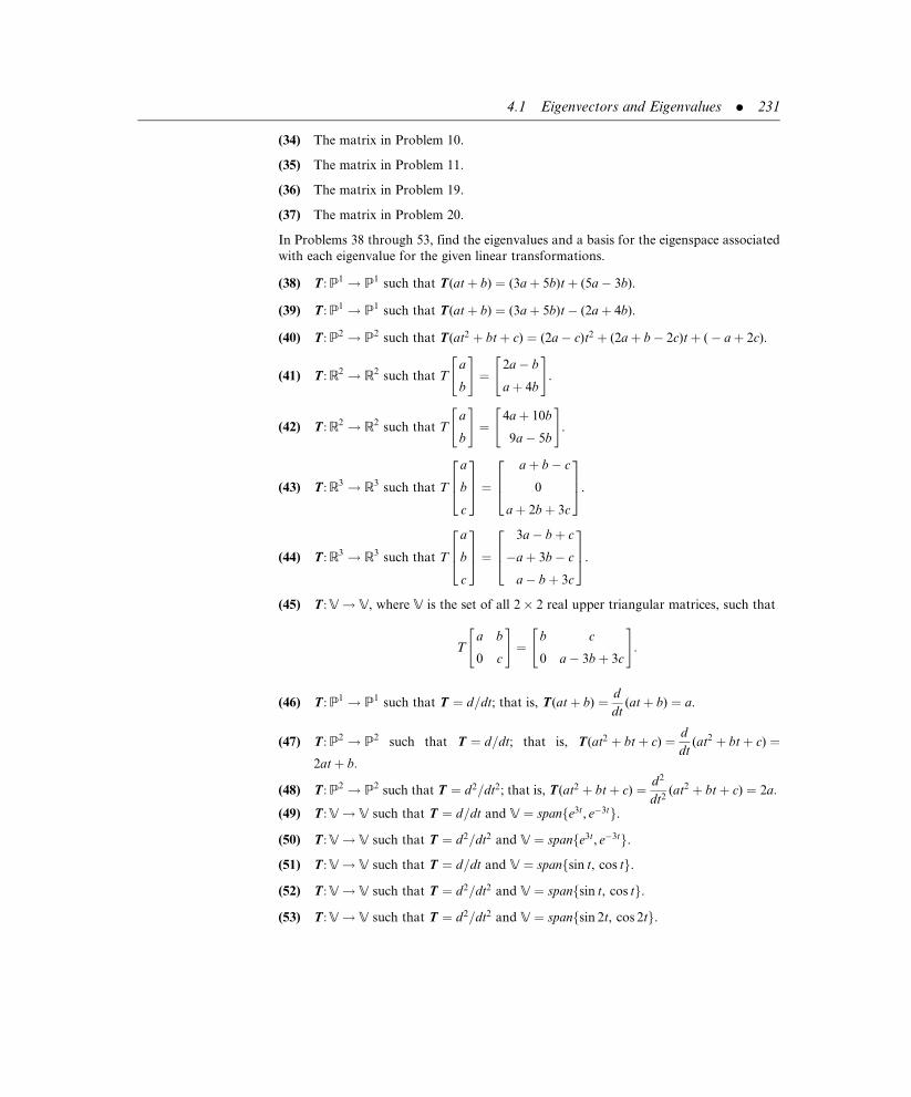
(34) The matrix in Problem 10.
(35) The matrix in Problem 11.
(36) The matrix in Problem 19.
(37) The matrix in Problem 20.
In Problems 38 through 53, find the eigenvalues and a basis for the eigenspace associated
with each eigenvalue for the given linear transformations.
(38) T: P1 ! P1 such that T(atþ b) ¼ (3aþ 5b)tþ (5a� 3b).
(39) T: P1 ! P1 such that T(atþ b) ¼ (3aþ 5b)t� (2aþ 4b).
(40) T: P2 ! P2 such that T(at2 þ btþ c) ¼ (2a� c)t2 þ (2aþ b� 2c)tþ (� aþ 2c).
(41) T: R2 ! R2 such that Ta
b
" #¼
2a� b
aþ 4b
" #.
(42) T: R2 ! R2 such that Ta
b
" #¼
4aþ 10b
9a� 5b
" #.
(43) T: R3 ! R3 such that T
a
b
c
264375 ¼
aþ b� c
0
aþ 2bþ 3c
264
375.
(44) T: R3 ! R3 such that T
a
b
c
264375 ¼
3a� bþ c
�aþ 3b� c
a� bþ 3c
264
375.
(45) T: V! V, where V is the set of all 2� 2 real upper triangular matrices, such that
Ta b
0 c
" #¼
b c
0 a� 3bþ 3c
" #:
(46) T: P1 ! P1 such that T ¼ d=dt; that is, T(atþ b) ¼ d
dt(atþ b) ¼ a.
(47) T: P2 ! P2 such that T ¼ d=dt; that is, T(at2 þ btþ c) ¼ d
dt(at2 þ btþ c) ¼
2atþ b:
(48) T: P2 ! P2 such that T ¼ d2=dt2; that is, T(at2 þ btþ c) ¼ d2
dt2(at2 þ btþ c) ¼ 2a:
(49) T: V! V such that T ¼ d=dt and V ¼ spanfe3t, e�3tg.
(50) T: V! V such that T ¼ d2=dt2 and V ¼ spanfe3t, e�3tg.
(51) T: V! V such that T ¼ d=dt and V ¼ spanfsin t, cos tg.
(52) T: V! V such that T ¼ d2=dt2 and V ¼ spanfsin t, cos tg.
(53) T: V! V such that T ¼ d2=dt2 and V ¼ spanfsin 2t, cos 2tg.
4.1 Eigenvectors and Eigenvalues . 231

(54) Consider the matrix
C ¼
0 1 0 . . . 0
0 0 1 . . . 0
..
. ... ..
. . .. ..
.
0 0 0 ...
1
�a0 �a1 �a2 . . . �an�1
2666664
3777775:
Use mathematical induction to prove that
det (C� lI) ¼ (� 1)n(ln þ an�1ln�1 þ . . .þ a2l2 þ a1lþ a0):
Deduce that the characteristic equation for this matrix is
ln þ an�1ln�1 þ . . .þ a2l2 þ a1lþ a0 ¼ 0:
The matrix C is called the companion matrix for this characteristic equation.
4.2 PROPERTIES OF EIGENVALUES AND EIGENVECTORS
The eigenvalues of a linear transformation T from a finite-dimensional vector
space to itself are identical to the eigenvalues of any matrix representation for T.
Consequently, we discover information about one by studying the other.
The kernel of A� lI is a vector space for any square matrix A, and all nonzero
vectors of this kernel are eigenvectors of A. A vector space is closed under scalar
multiplication, so kx is an eigenvector of A for any nonzero scalar k whenever x is
an eigenvector. Thus, in general, a matrix has a finite number of eigenvalues but
infinitely many eigenvectors. A vector space is also closed under vector addition,
so if x and y are two eigenvectors corresponding to the same eigenvalue l, then
so too is xþ y, providing this sum is not the zero vector.
The trace of a square matrix A, designated by tr(A), is the sum of the elements on
the main diagonal of A. In particular, the trace of
A ¼�1 2 0
�3 6 8
5 4 �2
24
35
is tr(A) ¼ �1þ 6þ (� 2) ¼ 3.
" Theorem 1. The sum of the eigenvalues of a matrix equals the trace of
the matrix. 3
We leave the proof of Theorem 1 as an exercise (see Problem 21). This result
provides a useful check on the accuracy of computed eigenvalues. If the sum of
the computed eigenvalues of a matrix do not equal the trace of the matrix, there
232 . Eigenvalues, Eigenvectors, and Differential Equations

is an error! Beware, however, that Theorem 1 only provides a necessary condi-
tion on eigenvalues, not a sufficient condition. That is, no conclusions can be
drawn from Theorem 1 if the sum of a set of eigenvalues equals the trace.
Eigenvalues of a matrix can be computed incorrectly and still have their sum
equal the trace of the matrix.
Example 1 Determine whether l1 ¼ 12 and l2 ¼ �4 are eigenvalues for
A ¼ 11 3
�5 �5
� �
Solution: Here tr(A) ¼ 11þ (� 5) ¼ 6 6¼ 8 ¼ l1 þ l2, so these numbers are not
the eigenvalues of A. The eigenvalues for this matrix are 10 and �4, and their
sum is the trace of A. &
The determinant of an upper (or lower) triangular matrix is the product of
elements on the main diagonal, so it follows immediately that
" Theorem 2. The eigenvalues of an upper or lower triangular matrix are
the elements on the main diagonal. 3
Example 2 The matrix
1 0 0
2 1 0
3 4 �1
24
35 is lower triangular, so its eigenvalues are
l1 ¼ l2 ¼ 1 and l3 ¼ �1. &
Once the eigenvalues of a matrix are known, one can determine immediately
whether the matrix is singular.
" Theorem 3. A matrix is singular if and only if it has a zero
eigenvalue. 3
Proof: A matrix A has a zero eigenvalue if and only if det (A� 0I) ¼ 0, or
(since 0I ¼ 0) if and only if det (A) ¼ 0, which is true (see Theorem 11 of
Appendix A) if and only if A is singular. &
A nonsingular matrix and its inverse have reciprocal eigenvalues and identical
eigenvectors.
" Theorem 4. If x is an eigenvector of an invertible matrix A correspond-
ing to the eigenvalue l, then x is also an eigenvector of A�1 correspond-
ing to the eigenvalue 1=l. 3
4.2 Properties of Eigenvalues and Eigenvectors . 233

Proof: Since A is invertible, Theorem 3 implies that l 6¼ 0; hence 1=l exists. We
have that Ax ¼ lx. Premultiplying both sides of this equation by A�1, we obtain
x ¼ lA�1x or A�1x ¼ (1=l)x
Thus, x is an eigenvector of A�1 with corresponding eigenvalue 1=l. &
We may combine Theorem 3 with Theorem 10 of Appendix A and Theorems 5
and 6 of Section 2.6 to obtain the following result.
" Theorem 5. The following statements are equivalent for an n� n
matrix A:
(i) A has an inverse.
(ii) A has rank n.
(iii) A can be transformed by elementary row operations to an
upper triangular matrix with only unity elements on the
main diagonal.
(iv) A has a nonzero determinant.
(v) Every eigenvalue of A is nonzero. 3
Multiplying the equation Ax ¼ lx by a scalar k, we obtain (kA)x ¼ (kl)x. Thus
we have proven Theorem 6.
" Theorem 6. If x is an eigenvector of A corresponding to the eigenvalue
l, then kl and x are a corresponding pair of eigenvalues and eigenvec-
tors of kA, for any nonzero scalar k. 3
Theorem 1 provides a relationship between the sum of the eigenvalues of a matrix
and its trace. There is also a relationship between the product of those eigen-
values and the determinant of the matrix. The proof of the next theorem is left as
an exercise (see Problem 22).
" Theorem 7. The product of all the eigenvalues of a matrix (counting
multiplicity) equals the determinant of the matrix. 3
Example 3 The eigenvalues of A ¼ 11 3
�5 �5
� �are l1 ¼ 10 and l2 ¼ �4. Here
det (A) ¼ �55þ 15 ¼ �40 ¼ l1l2. &
" Theorem 8. If x is an eigenvector of A corresponding to the eigenvalue
l, then ln and x are a corresponding pair of eigenvalues and eigenvectors
of An, for any positive integer n. 3
234 . Eigenvalues, Eigenvectors, and Differential Equations

Proof: We are given that Ax ¼ lx and we need to show that
Anx ¼ lnx (4:6)
We prove this last equality by mathematical induction on the power n. Equation
(4.6) is true for n ¼ 1 as a consequence of the hypothesis of the theorem. Now
assume that the proposition is true for n ¼ k� 1. Then
Ak�1x ¼ lk�1x
Premultiplying this equation by A, we have
A(Ak�1x) ¼ A (lk�1x)
or
Akx ¼ lk�1(Ax)
It now follows from the hypothesis of the theorem that
Akx ¼ lk�1(lx)
or
Akx ¼ lkx
which implies that the proposition is true for n ¼ k. Thus, Theorem 8 is proved
by mathematical induction. &
The proofs of the next two results are left as exercises for the reader (see
Problems 16 and 17).
" Theorem 9. If x is an eigenvector of A corresponding to the eigenvalue
l, then for any scalar c, l� c and x are a corresponding pair of eigen-
values and eigenvectors of A� cI. 3
" Theorem10. If l is an eigenvalue ofA, then l also an eigenvalue ofAT. &
Problems 4.2
(1) One eigenvalue of the matrix A ¼ 8 2
3 3
� �is known to be 2.
Determine the second eigenvalue by inspection.
(2) One eigenvalue of the matrix A ¼ 8 3
3 2
� �is known to be 0.7574 rounded to four
decimal places. Determine the second eigenvalue by inspection.
4.2 Properties of Eigenvalues and Eigenvectors . 235

(3) Two eigenvalues of a 3� 3 matrix are known to be 5 and 8. What can be said about
the third eigenvalue if the trace of the matrix is �4?
(4) Redo Problem 3 if �4 is the determinant of the matrix instead of its trace.
(5) The determinant of a 4� 4 matrix is 144 and two of its eigenvalues are known to be
�3 and 2. What can be said about the remaining eigenvalues?
(6) A 2� 2 matrix A is known to have the eigenvalues �3 and 4. What are the
eigenvalues of
(a) 2A, (b) 5A, (c) A� 3I, (d) Aþ 4I.
(7) A 3� 3 matrix A is known to have the eigenvalues �2, 2, and 4. What are the
eigenvalues of
(a) A2, (b) A3, (c) �3A, (d) Aþ 3I.
(8) A 2� 2 matrix A is known to have the eigenvalues �1 and 1. Find a matrix in
terms of A that has for its eigenvalues
(a) �2 and 2, (b) �5 and 5, (c) 1 and 1, (d) 2 and 4.
(9) A 3� 3 matrix A is known to have the eigenvalues 2, 3, and 4. Find a matrix in
terms of A that has for its eigenvalues
(a) 4, 6, and 8, (b) 4, 9, and 16, (c) 8, 27, and 64, (d) 0, 1, and 2.
(10) Verify Theorems 1 and 7 for A ¼ 8 3
3 2
� �.
(11) Verify Theorems 1 and 7 for A ¼1 3 6
�1 2 �1
2 1 7
24
35.
(12) What are the eigenvalues of A�1 for the matrices defined in Problems 10 and 11?
(13) Show by example that, in general, an eigenvalue of Aþ B is not the sum of an
eigenvalue of A with an eigenvalue of B.
(14) Show by example that, in general, an eigenvalue of AB is not the product of an
eigenvalue of A with an eigenvalue of B.
(15) Show by example that an eigenvector of A need not be an eigenvector of AT.
(16) Prove Theorem 9.
(17) Prove Theorem 10.
(18) The determinant of A� lI is known as the characteristic polynomial of A. For an
n� n matrix A it has the form
det (A� lI) ¼ (� 1)n ln þ an�1ln�1�
þ an�2ln�2 þ . . .þ a2l2 þ a1lþ a0
�,
where an�1, an�2, . . . , a2, a1, and a0 are constants that depend on the elements
of A. Show that (� 1)na0 ¼ det (A).
(19) (Problem 18 continued.) Convince yourself by considering arbitrary 2� 2, 3� 3,
and 4� 4 matrices that (� 1)an�1 ¼ tr(A).
236 . Eigenvalues, Eigenvectors, and Differential Equations

(20) Consider an n� n matrix A with eigenvalues l1, l2, . . . , ln, where some or all of the
eigenvalues may be equal. Each eigenvalue li(i ¼ 1, 2, . . . , n) is a root of the
characteristic polynomial; hence (l� li) must be a factor of that polynomial.
Deduce that det (A� lI) ¼ (� 1)n(l� l1)(l� l2) . . . (l� ln).
(21) Use the results of Problems 19 and 20 to prove Theorem 1.
(22) Use the results of Problems 18 and 20 to prove Theorem 7.
(23) The Cayley-Hamilton theorem states that every square matrix A satisfies its own
characteristic equation. That is, if the characteristic equation of A is
ln þ an�1ln�1 þ an�2ln�2 þ . . .þ a2l2 þ a1lþ a0 ¼ 0,
then
An þ an�1An�1 þ an�2A
n�2 þ . . .þ a2A2 þ a1Aþ a0I ¼ 0:
Verify the Cayley-Hamilton theorem for
(a)1 2
3 4
� �, (b)
1 2
2 4
� �, (c)
2 0 1
4 0 2
0 0 �1
24
35,
(d)
1 �1 2
0 3 2
2 1 2
24
35, (e)
1 0 0 0
0 �1 0 0
0 0 �1 0
0 0 0 1
2664
3775.
(24) Let the characteristic equation of a square matrix A be as given in Problem 23. Use
the results of Problem 18 to prove that A is invertible if and only if a0 6¼ 0.
(25) Let the characteristic equation of a square matrix A be given as in Problem 23. Use
the Cayley-Hamilton theorem to show that
A�1 ¼ �1
a0
An�1 þ an�1An�2
�þ . . .þ a2Aþ a1IÞ
when a0 6¼ 0.
(26) Use the result of Problem 25 to find the inverses, when they exist, for the matrices
defined in Problem 23.
4.3 DIAGONALIZATION OF MATRICES
We are ready to answer the question that motivated this chapter: Which linear
transformations can be represented by diagonal matrices and what bases gener-
ate such representations? Recall that different matrices represent the same linear
transformation if and only if those matrices are similar (Theorem 3 of Section
3.4). Therefore, a linear transformation has a diagonal matrix representation
if and only if any matrix representation of the transformation is similar to
a diagonal matrix.
4.3 Diagonalization of Matrices . 237

To establish whether a linear transformation T has a diagonal matrix represen-
tation, we first create one matrix representation for the transformation and then
determine whether that matrix is similar to a diagonal matrix. If it is, we say the
matrix is diagonalizable, in which case T has a diagonal matrix representation.
If a matrix A is similar to a diagonal matrix D, then the form of D is determined.
Both A and D have identical eigenvalues, and the eigenvalues of a diagonal
matrix (which is both upper and lower triangular) are the elements on its main
diagonal. Consequently, the main diagonal of D must be the eigenvalues of A. If,
for example,
A ¼ 1 2
4 3
� �
with eigenvalues �1 and 5, is diagonalizable, then A must be similar to either
�1 0
0 5
� �or
5 0
0 �1
� �
Now let A be an n� n matrix with n linearly independent eigenvectors x1, x2, . . . , xn
corresponding to the eigenvalues l1, l2, . . . , ln, respectively. Therefore,
Axj ¼ ljxj (4:7)
for j ¼ 1, 2, . . . , n. There are no restrictions on the multiplicity of the eigen-
values, so some or all of them may be equal. Set
M ¼ [ x1 x2 . . . xn ] and D ¼
l1 0 . . . 0
0 l2 . . . 0
..
. ... . .
. ...
0 0 . . . ln
26664
37775
Here M is called a modal matrix for A and D a spectral matrix for A. Now
AM ¼ A x1 x2 . . . xn½ �
¼ Ax1 Ax2 . . . Axn½ �
¼ l1x1 l2x2 . . . lnxn½ �
¼ x1 x2 . . . xn½ �D
¼MD (4:8)
Because the columns of M are linearly independent, the column rank of M is n,
the rank of M is n, and M�1 exists. Premultiplying equation (4.8) by M�1, we
obtain
D ¼M�1AM (4:9)
A matrix is
diagonalizable if it is
similar to a diagonal
matrix.
238 . Eigenvalues, Eigenvectors, and Differential Equations

Postmultiplying equation (4.8) by M�1, we have
A ¼MDM�1 (4:10)
Thus, A is similar to D. We can retrace our steps and show that if equation (4.10)
is satisfied, then M must be an invertible matrix having as its columns a set of
eigenvectors of A. We have proven the following result.
" Theorem 1. An n� n matrix is diagonalizable if and only if the matrix
possesses n linearly independent eigenvectors. 3
Example 1 Determine whether A ¼ 1 2
4 3
� �is diagonalizable.
Solution: Using the results of Example 3 of Section 4.1, we have l1 ¼ �1 and
l2 ¼ 5 as the eigenvalues of A with corresponding eigenspaces spanned by the
vectors
x1 ¼�1
1
� �and x2 ¼
1
2
� �
respectively. These two vectors are linearly independent, so A is diagonalizable.
We can choose either
M ¼ �1 1
1 2
� �or M ¼ 1 �1
2 1
� �
Making the first choice, we find
D ¼M�1AM ¼ 1
3
�2 1
1 1
� �1 2
4 3
� � �1 1
1 2
� �¼ �1 0
0 5
� �
Making the second choice, we find
D ¼M�1AM ¼ 1
3
1 1
�2 1
� �1 2
4 3
� �1 �1
2 1
� �¼ 5 0
0 �1
� �&
In general, neither the modal matrix M nor the spectral matrix D is unique.
However, once M is selected, then D is fully determined. The element of D
located in the jth row and jth column must be the eigenvalue corresponding to
the eigenvector in the jth column of M. In particular,
M ¼ [ x2 x1 x3 . . . xn ]
4.3 Diagonalization of Matrices . 239

is matched with
D ¼
l2 0 0 . . . 0
0 l1 0 . . . 0
0 0 l3 . . . 0
..
. ... ..
. . .. ..
.
0 0 0 . . . ln
26666664
37777775
while
M ¼ [ xn xn�1 . . . x1 ]
is matched with
D ¼
ln 0 . . . 0
0 ln�1 . . . 0
..
. ... . .
. ...
0 0 . . . l1
266664
377775
Example 2 Determine whether A ¼2 �1 0
3 �2 0
0 0 1
24
35 is diagonalizable.
Solution: Using the results of Example 6 of Section 4.1, we have
x1 ¼1
1
0
2435 and x2 ¼
0
0
1
2435
as a basis for the eigenspace corresponding to eigenvalue l ¼ 1 of multiplicity 2
and
x3 ¼1
3
0
2435
as a basis corresponding to eigenvalue l ¼ �1 of multiplicity 1. These three
vectors are linearly independent, so A is diagonalizable. If we choose
M ¼1 0 1
1 0 3
0 1 0
24
35, then M�1AM ¼
1 0 0
0 1 0
0 0 �1
24
35 &
240 . Eigenvalues, Eigenvectors, and Differential Equations

The process of determining whether a given set of eigenvectors is linearly
independent is simplified by the following two results.
" Theorem 2. Eigenvectors of a matrix corresponding to distinct eigen-
values are linearly independent. 3
Proof: Let l1, l2, . . . , lk denote the distinct eigenvalues of an n� n matrix A
with corresponding eigenvectors x1, x2, . . . , xk. If all the eigenvalues have multi-
plicity 1, then k ¼ n, otherwise k < n. We use mathematical induction to prove
that fx1, x2, . . . , xkg is a linearly independent set.
For k ¼ 1, the set fx1g is linearly independent because the eigenvector x1 cannot
be 0. We now assume that the set fx1, x2, . . . , xk�1g is linearly independent and
use this to show that the set fx1, x2, . . . , xk�1, xkg is linearly independent. This is
equivalent to showing that the only solution to the vector equation
c1x1 þ c2x2 þ . . .þ ck�1xk�1 þ ckxk ¼ 0 (4:11)
is c1 ¼ c2 ¼ . . . ¼ ck�1 ¼ ck ¼ 0.
Multiplying equation (4.11) on the left by A and using the fact that Axj ¼ ljxj
for j ¼ 1, 2, . . . , k, we obtain
c1l1x1 þ c2l2x2 þ . . .þ ck�1lk�1xk�1 þ cklkxk ¼ 0 (4:12)
Multiplying equation (4.11) by lk, we obtain
c1lkx1 þ c2lkx2 þ . . .þ ck�1lkxk�1 þ cklkxk ¼ 0 (4:13)
Subtracting equation (4.13) from (4.12), we have
c1(l1 � lk)x1 þ c2(l2 � lk)x2 þ . . .þ ck�1(lk�1 � lk)xk�1 ¼ 0
But the vectors x1, x2, . . . , xk�1f g are linearly independent by the induction
hypothesis, hence the coefficients in the last equation must all be 0; that is,
c1(l1 � lk) ¼ c2(l2 � lk) ¼ . . . ¼ ck�1(lk�1 � lk) ¼ 0
from which we imply that c1 ¼ c2 ¼ . . . ¼ ck�1 ¼ 0, because the eigenvalues are
distinct. Equation (4.11) reduces to ckxk ¼ 0 and because xk is an eigenvector, and
therefore nonzero, we also conclude that ck ¼ 0, and the proof is complete. &
It follows from Theorems 1 and 2 that any n� n real matrix having n distinct real
roots of its characteristic equation, that is a matrix having n eigenvalues all of
multiplicity 1, must be diagonalizable. (See, in particular, Example 1.)
4.3 Diagonalization of Matrices . 241

Example 3 Determine whether A ¼2 0 0
�3 3 0
2 �1 4
24
35 is diagonalizable.
Solution: The matrix is lower triangular so its eigenvalues are the elements on
the main diagonal, namely 2, 3, and 4. Every eigenvalue has multiplicity 1, hence
A is diagonalizable. &
" Theorem 3. If l is an eigenvalue of multiplicity k of an n� n matrix A,
then the number of linearly independent eigenvectors of A associated
with l is n� r(A� lI), where r denotes rank. 3
Proof: The eigenvectors of A corresponding to the eigenvalue l are all nonzero
solutions of the vector equation (A� lI)x ¼ 0. This homogeneous system is
consistent, so by Theorem 3 of Section 2.6 the solutions will be in terms of
n� r(A� lI) arbitrary unknowns. Since these unknowns can be picked inde-
pendently of each other, they generate n� r(A� lI) linearly independent
eigenvectors. &
In Example 2, A is a 3� 3 matrix (n ¼ 3) and l ¼ 1 is an eigenvalue of multi-
plicity 2. In this case,
A� (1)I ¼ A� I ¼1 �1 0
3 �3 0
0 0 0
24
35
can be transformed into row-reduced form (by adding to the second row �3
times the first row)
1 �1 0
0 0 0
0 0 0
24
35
having rank 1. Thus, n� r(A� I) ¼ 3� 1 ¼ 2 and A has two linearly inde-
pendent eigenvectors associated with l ¼ 1. Two such vectors are exhibited in
Example 2.
Example 4 Determine whether A ¼ 2 1
0 2
� �is diagonalizable.
Solution: The matrix is upper triangular so its eigenvalues are the elements on
the main diagonal, namely, 2 and 2. Thus, A is 2� 2 matrix with one eigenvalue
of multiplicity 2. Here
A� 2I ¼ 0 1
0 0
� �
242 . Eigenvalues, Eigenvectors, and Differential Equations
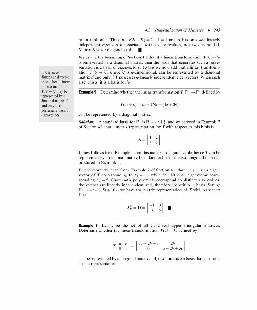
has a rank of 1. Thus, n� r(A� 2I) ¼ 2� 1 ¼ 1 and A has only one linearly
independent eigenvector associated with its eigenvalues, not two as needed.
Matrix A is not diagonalizable. &
We saw in the beginning of Section 4.1 that if a linear transformation T: V! V
is represented by a diagonal matrix, then the basis that generates such a repre-
sentation is a basis of eigenvectors. To this we now add that a linear transform-
ation T: V! V, where V is n-dimensional, can be represented by a diagonal
matrix if and only if T possesses n-linearly independent eigenvectors. When such
a set exists, it is a basis for V.
Example 5 Determine whether the linear transformation T: P1 ! P1 defined by
T(atþ b) ¼ (aþ 2b)tþ (4aþ 3b)
can be represented by a diagonal matrix.
Solution: A standard basis for P1 is B ¼ t, 1f g, and we showed in Example 7
of Section 4.1 that a matrix representation for T with respect to this basis is
A ¼ 1 2
4 3
� �
It now follows from Example 1 that this matrix is diagonalizable; hence T can be
represented by a diagonal matrix D, in fact, either of the two diagonal matrices
produced in Example 1.
Furthermore, we have from Example 7 of Section 4.1 that �tþ 1 is an eigen-
vector of T corresponding to l1 ¼ �1 while 5tþ 10 is an eigenvector corre-
sponding l2 ¼ 5. Since both polynomials correspond to distinct eigenvalues,
the vectors are linearly independent and, therefore, constitute a basis. Setting
C ¼ f�tþ 1, 5tþ 10g, we have the matrix representation of T with respect to
C as
ACC ¼ D ¼ �1 0
0 5
� �&
Example 6 Let U be the set of all 2� 2 real upper triangular matrices.
Determine whether the linear transformation T: U! U defined by
Ta b
0 c
� �¼ 3aþ 2bþ c 2b
0 aþ 2bþ 3c
� �
can be represented by a diagonal matrix and, if so, produce a basis that generates
such a representation.
If V is an n-
dimensional vector
space, then a linear
transformation
T: V! V may be
represented by a
diagonal matrix if
and only if T
possesses a basis of
eigenvectors.
4.3 Diagonalization of Matrices . 243

Solution: U is closed under addition and scalar multiplication, so it is a sub-
space of M2�2. A simple basis for U is given by
B ¼ 1 0
0 0
� ��,
0 1
0 0
� �,
0 0
0 1
� ��
With respect to these basis vectors,
T1 0
0 0
" #¼
3 0
0 1
" #¼ 3
1 0
0 0
" #þ 0
0 1
0 0
" #þ 1
0 0
0 1
" #$
3
0
1
26643775
T0 1
0 0
" #¼
2 2
0 2
" #¼ 2
1 0
0 0
" #þ 2
0 1
0 0
" #þ 2
0 0
0 1
" #$
2
2
2
26643775
T0 0
0 1
" #¼
1 0
0 3
" #¼ 1
1 0
0 0
" #þ 0
0 1
0 0
" #þ 3
0 0
0 1
" #$
1
0
3
26643775
and a matrix representation for T is
A ¼3 2 1
0 2 0
1 2 3
24
35
The eigenvalues of this matrix are 2, 2, and 4. Even though the eigenvalues are
not all distinct, the matrix still has three linearly independent eigenvectors,
namely,
x1 ¼�2
1
0
24
35, x2 ¼
�1
0
1
24
35, and x3 ¼
1
0
1
2435
Thus, A is diagonalizable and, therefore, T has a diagonal matrix representation.
Setting
M ¼�2 �1 1
1 0 0
0 1 1
24
35, we have D ¼M�1AM ¼
2 0 0
0 2 0
0 0 4
24
35
which is one diagonal representation for T.
The vectors x1, x2, and x3 are coordinate representations with respect to the B
basis for
244 . Eigenvalues, Eigenvectors, and Differential Equations

�2
1
0
264
375$ (� 2)
1 0
0 0
" #þ 1
0 1
0 0
" #þ 0
0 0
0 1
" #¼�2 1
0 0
" #
�1
0
1
264
375$ (� 1)
1 0
0 0
" #þ 0
0 1
0 0
" #þ 1
0 0
0 1
" #¼�1 0
0 1
" #
1
0
1
264375$ 1
1 0
0 0
" #þ 0
0 1
0 0
" #þ 1
0 0
0 1
" #¼
1 0
0 1
" #
The set
C ¼ �2 1
0 0
� ��,�1 0
0 1
� �,
1 0
0 1
� ��
is a basis of eigenvectors of T for the vector space U. A matrix representation of
T with respect to the C basis is the diagonal matrix D. &
Problems 4.3
In Problems 1 through 11, determine whether the matrices are diagonalizable. If they are,
identify a modal matrix M and calculate M�1AM.
(1) A ¼ 2 �3
1 �2
� �. (2) A ¼ 4 3
3 �4
� �.
(3) A ¼ 3 1
�1 5
� �. (4) A ¼
1 1 1
0 1 0
0 0 1
24
35.
(5) A ¼1 0 0
2 �3 3
1 2 2
24
35. (6) A ¼
5 1 2
0 3 0
2 1 5
24
35.
(7) A ¼1 2 3
2 4 6
3 6 9
24
35. (8) A ¼
3 �1 1
�1 3 �1
1 �1 3
24
35.
(9) A ¼7 3 3
0 1 0
�3 �3 1
24
35. (10) A ¼
3 1 0
0 3 1
0 0 3
24
35.
(11) A ¼3 0 0
0 3 1
0 0 3
24
35.
In Problems 12 through 21, determine whether the linear transformations can be represented
by diagonal matrices and, if so, produce bases that will generate such representations.
4.3 Diagonalization of Matrices . 245

(12) T: P1 ! P1 defined by T(atþ b) ¼ (2a� 3b)tþ (a� 2b).
(13) T: P1 ! P1 defined by T(atþ b) ¼ (4aþ 3b)tþ (3a� 4b).
(14) T: P2 ! P2 defined by
T(at2 þ btþ c) ¼ at2 þ (2a� 3bþ 3c)tþ (aþ 2bþ 2c):
(15) T: P2 ! P2 defined by
T(at2 þ btþ c) ¼ (5aþ bþ 2c)t2 þ 3btþ (2aþ bþ 5c):
(16) T: P2 ! P2 defined by
T(at2 þ btþ c) ¼ (3aþ b)t2 þ (3bþ c)tþ 3c:
(17) T: U! U where U is the set of all 2� 2 real upper triangular matrices and
Ta b
0 c
� �¼
aþ 2bþ 3c 2aþ 4bþ 6c
0 3aþ 6bþ 9c
� �:
(18) T: U! U where U is the set of all 2� 2 real upper triangular matrices and
Ta b
0 c
� �¼
7aþ 3bþ 3c b
0 �3a� 3bþ c
� �:
(19) T: W!W where W is the set of all 2� 2 real lower triangular matrices and
Ta 0
b c
� �¼
3a� bþ c 0
�aþ 3b� c a� bþ 3c
� �:
(20) T: R3 ! R3 defined by T
a
b
c
2435 ¼ c
a
b
2435.
(21) T: R3 ! R3 defined by T
a
b
c
264375 ¼ 3aþ b
3bþ c
c
264
375.
4.4 THE EXPONENTIAL MATRIX
In this section and the next section (Power Methods), we will use eigenvalues and
eigenvectors extensively and conclude our chapter with sections dealing with
differential equations.
One of the most important functions in the calculus is the exponential function
ex. It should not be surprising, therefore, to find that the ‘‘exponentials of
matrices’’ are equally useful and important.
246 . Eigenvalues, Eigenvectors, and Differential Equations

To develop this idea, we extend the idea of Maclaurin series to include matrices.
As we further our discussion, we will make reference to the Jordan canonical
form (see Appendix B).
We recall that this function can be written as a Maclaurin series:
ex ¼X1k¼0
xk
k!¼ 1þ xþ x2
2!þ x3
3!þ . . . (4:14)
Then we can use this expansion to define the exponential of a square matrix A as
eA ¼X1k¼0
Ak
k!¼ IþA
1!þA2
2!þA3
3!þ . . . (4:15)
Equation (4.14) converges for all values of the variable x; analogously, it can be
shown that equation (4.15) converges for all square matrices A, although the
actual proof is well beyond the scope of this book. Using equation (4.14), we can
easily sum the right side of equation (4.15) for any diagonal matrix.
Example 1 For A ¼ 2 0
0 �0:3
� �, we have
eA ¼1 0
0 1
" #þ 1
1!
2 0
0 �0:3
" #þ 1
2!
2 0
0 �0:3
" #2
þ 1
3!
2 0
0 �0:3
" #3
þ . . .
¼1 0
0 1
" #þ
2=1! 0
0 (� 0:3)=1!
" #þ
(2)2=2! 0
0 (� 0:3)2=2!
" #
þ(2)3=3! 0
0 (� 0:3)3=3!
" #þ . . .
¼
X1k¼0
2k
k!0
0X1k¼0
(� 0:3)k
k!
266664
377775 ¼
e2 0
0 e�0:3
" #&
In general, if D is the diagonal matrix
D ¼
l1 0 . . . 0
0 l2 . . . 0
..
. ... . .
. ...
0 0 . . . ln
26664
37775
The exponential of a
square matrix A is
defined by the
infinite series
eA ¼X1k¼0
Ak
k!
¼ IþA
1!þA2
2!
þA3
3!þ . . . :
4.4 The Exponential Matrix . 247

then
eD ¼
el1 0 . . . 0
0 el2 . . . 0
..
. ... . .
. ...
0 0 . . . eln
2664
3775 (4:16)
Example 2 Find eD for D ¼1 0 0
0 2 0
0 0 2
24
35.
Solution:
eD ¼e1 0 0
0 e2 0
0 0 e2
24
35 &
If a square matrix A is not diagonal, but diagonalizable, then we know from our
work in Section 4.3 that there exists a modal matrix M such that
A ¼MDM�1 (4:17)
where D is a diagonal matrix. It follows that
A2 ¼ AA ¼ (MDM�1)(MDM�1) ¼MD(M�1M)DM�1
¼MD(I)DM�1 ¼MD2M�1
A3 ¼ A2A ¼ (MD2M�1)(MDM�1) ¼MD2(M�1M)DM�1 ¼MD2(I)DM�1
¼MD3M�1
and, in general,
An ¼MDnM�1 (4:18)
for any positive integer n. Consequently,
eA ¼X1k¼0
Ak
k!¼X1k¼0
MDkM�1
k!¼M
X1k¼0
Dk
k!
!M�1 ¼MeDM�1 (4:19)
Example 3 Find eA for A ¼ 1 2
4 3
� �:
Solution: The eigenvalues of A are �1 and 5 with corresponding eigenvectors
1
�1
� �and
1
2
� �. Here,
To calculate the
exponential of a
diagonal matrix,
replace each
diagonal element by
the exponential of
that diagonal
element.
248 . Eigenvalues, Eigenvectors, and Differential Equations

M ¼ 1 1
�1 2
� �, M�1 ¼ 2=3 �1=3
1=3 1=3
� �, and D ¼ �1 0
0 5
� �:
It follows first from equation (4.19) and then from (4.16) that
eA ¼MeDM�1 ¼1 1
�1 2
� �e�1 0
0 e5
" #2=3 �1=3
1=3 1=3
" #
¼ 1
3
2e�1 þ e5 �e�1 þ e5
�2e�1 þ 2e5 e�1 þ 2e5
" #&
Even if a matrix A is not diagonalizable, it is still similar to a matrix J in Jordan
canonical form (see Appendix B). That is, there exists a generalized modal matrix
M such that
A ¼MJM�1 (4:20)
Repeating the derivation of (4.18) and (4.19), with J replacing D, we obtain
eA ¼MeJM�1 (4:21)
Thus, once we know how to calculate eJ for a matrix J in Jordan canonical form,
we can use equation (4.21) to find eA for any square matrix A.
A matrix J in Jordan canonical form has the block diagonal pattern
J ¼
J1 0 . . . 0
0 J2 . . . 0
..
. ... . .
. ...
0 0 . . . Jr
26664
37775 (4:22)
with each Ji(i ¼ 1, 2, . . . , r) being a Jordan block of the form
Ji ¼
li 1 0 . . . 0 0
0 li 1 . . . 0 0
..
. ... ..
. . .. . .
. . ..
0 0 0 . . . li 1
0 0 0 . . . 0 li
2666664
3777775 (4:23)
Powers of a matrix in Jordan canonical form are relatively easy to calculate.
J2 ¼ JJ ¼
J1 0 . . . 0
0 J2 . . . 0
..
. ... . .
. ...
0 0 . . . Jr
266664
377775
J1 0 . . . 0
0 J2 . . . 0
..
. ... . .
. ...
0 0 . . . Jr
266664
377775 ¼
J21 0 . . . 0
0 J22 . . . 0
..
. ... . .
. ...
0 0 . . . J2r
2666664
3777775
If A is similar to a
matrix J in Jordan
canonical form, so
that A ¼MJM�1
for a generalized
modal matrix M,
then eA ¼MeJM�1.
(See Appendix B.)
4.4 The Exponential Matrix . 249

J3 ¼ JJ2 ¼
J1 0 . . . 0
0 J2 . . . 0
..
. ... . .
. ...
0 0 . . . Jr
26664
37775
J21 0 . . . 0
0 J22 . . . 0
..
. ... . .
. ...
0 0 . . . J2r
26664
37775 ¼
J31 0 . . . 0
0 J32 . . . 0
..
. ... . .
. ...
0 0 . . . J3r
26664
37775
and, in general,
Jk ¼
Jk1 0 . . . 0
0 Jk2 . . . 0
..
. ... . .
. ...
0 0 . . . Jkr
266664
377775
for any positive integer value of k. Consequently,
eJ ¼X1k¼0
Jk
k!¼X1k¼0
1
k!
Jk1 0 . . . 0
0 Jk2 . . . 0
..
. ... . .
. ...
0 0 . . . Jkr
2666664
3777775 ¼
X1k¼0
Jk1
k!0 . . . 0
0X1k¼0
Jk2
k!. . . 0
..
. ... . .
. ...
0 0 . . .X1k¼0
Jkr
k!
26666666666664
37777777777775
¼
eJ1 0 . . . 0
0 eJ2 . . . 0
..
. ... . .
. ...
0 0 . . . eJr
266664
377775 (4:24)
Thus, once we know how to calculate the exponential of a Jordan block, we can
use equation (4.24) to find eJ for a matrix J in Jordan canonical form and then
equation (4.21) to obtain eA for a square matrix A.
A 1� 1 Jordan block has the form [l] for some scalar l. Such a matrix is
a diagonal matrix, indeed all 1� 1 matrices are, by default, diagonal matrices,
and it follows directly from equation (4.16) that e[l] ¼ [el]. All other Jordan
blocks have superdiagonal elements, which are all ones. For p� p Jordan block
in the form of (4.23), we can show by direct calculations that each successive
power has one additional diagonal of nonzero entries, until all elements above
the main diagonal become nonzero. On each diagonal, the entries are identical. If
we designate the nth power of a Jordan block as the matrix ani j
h i, then the entries
can be expressed compactly in terms of derivatives as
ani, iþj ¼
1
j!
dj
dlji
lni
� �for j ¼ 0, 1, . . . , n
0 otherwise
8<:
250 . Eigenvalues, Eigenvectors, and Differential Equations

Equation (4.15) then reduces to
eJi ¼ eli
11
1!
1
2!
1
3!. . .
1
(p� 1)!
0 11
1!
1
2!. . .
1
(p� 2)!
0 0 11
1!. . .
1
(p� 3)!
. . . . . . . . . . . . . . . . . .
0 0 0 0 . . . 1
266666666666664
377777777777775
(4:25)
Example 4 Find eJ for J ¼2t 1 0
0 2t 1
0 0 2t
24
35.
Solution: J is a single Jordan block with diagonal elements li ¼ 2t. For this
matrix, equation (4.25) becomes
eJ ¼ e2t
1 1 1=2
0 1 1
0 0 1
24
35 &
Example 5 Find eJ for J ¼
2 0 0 0 0 0
0 3 0 0 0 0
0 0 1 1 0 0
0 0 0 1 1 0
0 0 0 0 1 1
0 0 0 0 0 1
2666666664
3777777775
Solution: J is in the Jordan canonical form
J ¼J1 0 0
0 J2 0
0 0 J3
264
375
with J1 ¼ [2] and J2 ¼ [3] both of order 1� 1, and
J3 ¼
1 1 0 0
0 1 1 0
0 0 1 1
0 0 0 1
26664
37775
The exponential of a
matrix in Jordan
canonical form
(4.22) has block
diagonal form
(4.24), with the
exponential of each
Jordan block given
by (4.25).
4.4 The Exponential Matrix . 251

Here,
eJ1 ¼ e2� �
, eJ2 ¼ e3� �
, and
eJ3 ¼ e1
1 1 1=2 1=6
0 1 1 1=2
0 0 1 1
0 0 0 1
26666664
37777775 ¼
e e e=2 e=6
0 e e e=2
0 0 e e
0 0 0 e
26666664
37777775
Then,
eJ ¼
e2 0 0 0 0 0
0 e3 0 0 0 0
0 0 e e e=2 e=6
0 0 0 e e e=2
0 0 0 0 e e
0 0 0 0 0 e
266666666664
377777777775
&
Example 6 Find eA for A ¼0 4 2
�3 8 3
4 �8 �2
24
35.
Solution: A canonical basis for this matrix has one chain of length 2:
x2 ¼ 0 0 1½ �T and x1 ¼ 2 3 �4½ �T, and one chain of length 1:
y1 ¼ 2 1 0½ �T, each corresponding to the eigenvalue 2. Setting
M ¼2 2 0
1 3 0
0 �4 1
24
35 and J ¼
2 0 0
0 2 1
0 0 2
24
35
we have A ¼MJM�1. Here J contains two Jordan blocks, the 1� 1 matrix
J1 ¼ [2] and the 2� 2 matrix J2 ¼2 1
0 2
� �. We have,
eJ1 ¼ e2� �
, eJ2 ¼ e21 1
0 1
� �¼ e2 e2
0 e2
" #
eJ ¼ 65 ¼e2 0 0
0 e2 e2
0 0 e2
264
375
252 . Eigenvalues, Eigenvectors, and Differential Equations

eA ¼MeJM�1 ¼2 2 0
1 3 0
0 �4 1
264
375 e2 0 0
0 e2 e2
0 0 e2
264
375 3=4 �1=2 0
�1=4 1=2 0
�1 2 1
264
375
¼e2
�1 4 2
�3 7 3
4 �8 �3
264
375 &
Two important properties of the exponential of a matrix are given in the next
theorems.
" Theorem 1. e0 ¼ I, where 0 is the n� n zero matrix and I is the n� n
identity matrix. 3
Proof: In general,
eA ¼X1k¼0
Ak
k!¼ I þ
X1k¼1
Ak
k!(4:26)
With A ¼ 0, we have
e0 ¼ I þX1k¼1
0k
k!¼ I
" Theorem 2. eA� ��1¼ e�A. 3
Proof:
eAe�A ¼X1k¼0
Ak
k!
" # X1k¼0
(� A)k
k!
" #
¼ I þ Aþ A2
2!þ A3
3!þ . . .
� �I þ Aþ A2
2!þ A3
3!þ . . .
� �
¼ IIþ A[1� 1]þ A2 1
2!� 1þ 1
2!
� �þ A3 � 1
3!þ 1
2!� 1
2!þ 1
3!
� �þ . . .
¼ I
Thus, e�A is the inverse of eA.
We conclude from Theorem 2 that eA is always invertible even when A is not. To
calculate e�A directly, set B ¼ �A, and then determine eB.
To calculate eAt,
where A is a square
constant matrix and
t is a variable, set
B ¼ At and
calculate eB.
4.4 The Exponential Matrix . 253
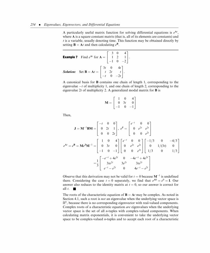
A particularly useful matrix function for solving differential equations is eAt,
where A is a square constant matrix (that is, all of its elements are constants) and
t is a variable, usually denoting time. This function may be obtained directly by
setting B ¼ At and then calculating eB.
Example 7 Find eAt for A ¼3 0 4
1 2 1
�1 0 �2
24
35.
Solution: Set B ¼ At ¼3t 0 4t
t 2t t
�t 0 �2t
24
35.
A canonical basis for B contains one chain of length 1, corresponding to the
eigenvalue �t of multiplicity 1, and one chain of length 2, corresponding to the
eigenvalue 2t of multiplicity 2. A generalized modal matrix for B is
M ¼1 0 4
0 3t 0
�1 0 �1
24
35
Then,
J ¼M�1BM ¼�t 0 0
0 2t 1
0 0 2t
264
375, eJ ¼
e�t 0 0
0 e2t e2t
0 0 e2t
264
375
eAt ¼ eB ¼MeJM�1 ¼1 0 4
0 3t 0
�1 0 �1
264
375 e�t 0 0
0 e2t e2t
0 0 e2t
264
375 �1=3 0 �4=3
0 1=(3t) 0
1=3 0 1=3
264
375
¼ 1
3
�e�t þ 4e2t 0 �4e�t þ 4e2t
3te2t 3e2t 3te2t
e�t � e2t 0 4e�t � e2t
264
375
Observe that this derivation may not be valid for t ¼ 0 because M�1 is undefined
there. Considering the case t ¼ 0 separately, we find that eA0 ¼ e0 ¼ I. Our
answer also reduces to the identity matrix at t ¼ 0, so our answer is correct for
all t. &
The roots of the characteristic equation of B ¼ At may be complex. As noted in
Section 4.1, such a root is not an eigenvalue when the underlying vector space is
Rn, because there is no corresponding eigenvector with real-valued components.
Complex roots of a characteristic equation are eigenvalues when the underlying
vector space is the set of all n-tuples with complex-valued components. When
calculating matrix exponentials, it is convenient to take the underlying vector
space to be complex-valued n-tuples and to accept each root of a characteristic
254 . Eigenvalues, Eigenvectors, and Differential Equations

equation as an eigenvalue. Consequently, a generalized modal matrix M may
contain complex-valued elements.
If A is a real matrix and t a real-valued variable, then Bt is real-valued. Because
all integral powers of matrices with real elements must also be real, it follows
from equation (4.26) that eB must be real. Thus, even if J and M have complex-
valued elements, the product eB ¼MeJM�1 must be real. Complex roots of the
characteristic equation of a real matrix must appear in conjugate pairs, which
often can be combined into real-valued quantities by using Euler’s relations:
cos u ¼ eiu þ e�iu
2and sin u ¼ eiu � e�iu
2i
Example 8 Find eAt for A ¼ 0 1
�1 0
� �.
Solution: Set B ¼ At ¼ 0 t
�t 0
� �:
The eigenvalues of B are l1 ¼ it and l2 ¼ �it, with corresponding eigenvectors
1 i½ �T and 1 �i½ �T, respectively. Thus,
M ¼ 1 1
i �i
� �, J ¼ it 0
0 �it
� �
and
eAt ¼ eB ¼1 1
i �i
� �eit 0
0 e�it
� �1=2 �i=2
1=2 i=2
� �
¼eit þ e�it
2eit � e�it
2i
� eit � e�it
2i
eit þ e�it
2
264
375 ¼ cos t sin t
� sin t cos t
� �&
If the eigenvalues of B ¼ At are not pure imaginary but rather complex numbers
of the form bþ iu and b� iu, then the algebraic operations needed to simplify eB
are more tedious. Euler’s relations remain applicable, but as part of the following
identities:
e bþiu þ e b�iu
2¼ e be iu þ e be�iu
2¼ e b e iu þ e �iuð Þ
2¼ e b cos u
and
e bþ iu � e b� iu
2i¼ e be iu � e be �iu
2i¼ e b e iu � e �iuð Þ
2i¼ e b sin u
4.4 The Exponential Matrix . 255

The exponential of a matrix is useful in matrix calculus for the same reason the
exponential function is so valuable in the calculus: the derivative of eAt is closely
related to the function itself. The derivative of a matrix is obtained by differen-
tiating each element in the matrix. Thus, a matrix C ¼ [cij] has a derivative if and
only if each element cij has a derivative, in which case, we write
_CC(t) ¼ dC(t)
dt¼ dci j(t)
dt
� �(4:27)
Example 9 If C(t) ¼t2 sin t
ln t et2
" #, then
_CC(t) ¼ dC(t)
dt¼
d(t2)
dt
d( sin t)
dt
d( ln t)
dt
d(et2 )
dt
26664
37775 ¼ 2t cos t
1=t 2tet2
" #&
" Theorem 3. If A is a constant matrix, thendeAt
dt¼ AeAt ¼ eAtA. 3
Proof:
deAt
dt¼ d
dt
X1k¼0
(At)k
k!
!¼ d
dt
X1k¼0
Aktk
k!
!¼X1k¼0
d
dt
Aktk
k!
¼X1k¼0
kAktk�1
k!
¼ 0þX1k¼1
A Ak�1tk�1
(k� 1)!¼ A
X1k¼1
Ak�1tk�1
(k� 1)!
!
¼AX1j¼0
Ajtj
j!
!¼ A
X1j¼0
(A t)j
j!
!¼ AeAt
If we factor A on the right, instead of the left, we obtain the other identity.
By replacing A with �A in Theorem 3, we obtain:
" Corollary 1. If A is a constant matrix, thende�At
dt¼ �AeAt ¼ �eAtA. 3
The derivative of a
matrix is obtained
by differentiating
each element in the
matrix.
256 . Eigenvalues, Eigenvectors, and Differential Equations

Problems 4.4
In Problems 1 through 30, find the exponential of each matrix.
(1)�1 0
0 4
� �. (2)
2 0
0 3
� �. (3)
�7 0
0 �7
� �.
(4)0 0
0 0
� �. (5)
�7 1
0 �7
� �. (6)
2 1
0 2
� �.
(7)3 1
0 3
� �. (8)
0 1
0 0
� �. (9)
2 0 0
0 3 0
0 0 4
24
35.
(10)
1 0 0
0 �5 0
0 0 �1
24
35. (11)
2 0 0
0 2 0
0 0 2
24
35. (12)
2 1 0
0 2 1
0 0 2
24
35.
(13)
�1 1 0
0 �1 1
0 0 �1
24
35. (14)
0 1 0
0 0 1
0 0 0
24
35. (15)
�1 0 0
0 �1 1
0 0 �1
24
35.
(16)
2 0 0
0 2 1
0 0 2
24
35. (17)
1 0 0 0
0 5 0 0
0 0 �5 0
0 0 0 3
2664
3775. (18)
�5 0 0 0
0 �5 0 0
0 0 �5 0
0 0 0 �5
2664
3775.
(19)
�5 0 0 0
0 �5 0 0
0 0 �5 1
0 0 0 �5
2664
3775. (20)
�5 0 0 0
0 �5 1 0
0 0 �5 1
0 0 0 �5
2664
3775.
(21)
�5 0 0 0
0 �5 1 0
0 0 �5 1
0 0 0 �5
2664
3775. (22)
�5 1 0 0
0 �5 1 0
0 0 �5 1
0 0 0 �5
2664
3775.
(23)
2 0 1
0 2 0
0 0 2
24
35. (24)
1 3
4 2
� �. (25)
4 �1
1 2
� �.
(26)
1 1 2
�1 3 4
0 0 2
24
35. (27)
p p=3 �p
0 p p=20 0 p
24
35. (28)
2 1 0
0 2 2
0 0 2
24
35.
(29)
1 0 0
2 3 �1
1 1 1
24
35. (30)
2 1 0 0
0 2 0 0
0 0 2 7
0 0 �1 1
2664
3775.
(31) Verify Theorem 2 for A ¼ 1 3
0 1
� �.
(32) Verify Theorem 2 for A ¼ 0 1
�64 0
� �.
4.4 The Exponential Matrix . 257

(33) Verify Theorem 2 for A ¼0 1 0
0 0 1
0 0 0
24
35. What is the inverse of A?
(34) Find eAeB, eBeA, and eAþB when
A ¼ 1 1
0 0
� �and B ¼ 0 1
0 1
� �,
and show that eAþB 6¼ eAeB 6¼ eBeA.
(35) Find two matrices A and B such that eAeB ¼ eAþB.
(36) Using equation (4.15) directly, prove that eAeB ¼ eAþB when A and B commute.
In Problems 37 through 55, find eAt for the given matrix A.
(37)4 4
3 5
� �. (38)
2 1
�1 �2
� �. (39)
4 1
�1 2
� �.
(40)0 1
�14 9
� �. (41)
�3 2
2 �6
� �. (42)
�10 6
6 �10
� �.
(43)2 1
0 2
� �. (44)
0 1 0
0 0 1
0 0 0
24
35. (45)
1 0 0
4 1 2
�1 4 �1
24
35.
(46)
�1 1 0
0 �1 1
0 0 �1
24
35. (47)
4 1 0
0 4 0
0 0 4
24
35. (48)
2 1 0
0 2 0
0 0 �1
24
35.
(49)
2 3 0
�1 �2 0
1 1 1
24
35. (50)
3 1 0
�1 1 0
1 2 2
24
35. (51)
5 �2 2
2 0 1
�7 5 �2
24
35.
(52)0 1
�64 0
� �. (53)
2 5
�1 �2
� �. (54)
0 1
�25 �8
� �.
(55)3 1
�2 5
� �.
(56) Verify Theorem 3 for the matrix A given in Example 7.
(57) Verify Theorem 3 for the matrix A given in Example 8.
(58) Using the formula
d[A(t)B(t)]
dt¼ dA(t)
dt
B(t)þ A(t)
dB(t)
dt
,
derive a formula for differentiating A2(t). Use this formula to find dA2(t)=dt
when
258 . Eigenvalues, Eigenvectors, and Differential Equations

A(t) ¼ t 2t2
4t3 et
� �,
and show that dA2(t)=dt 6¼ 2A(t)dA(t)=dt. Therefore, the power rule of differentiation
does not hold for matrices unless a matrix commutes with its derivative.
4.5 POWER METHODS
The analytic methods described in Section 4.1 are impractical for calculating the
eigenvalues and eigenvectors of matrices of large order. Determining the char-
acteristic equations for such matrices involves enormous effort, and finding its
roots algebraically is usually impossible. Instead, iterative methods that lend
themselves to computer implementation are used. Ideally, each iteration yields a
new approximation, which converges to an eigenvalue and the corresponding
eigenvector.
The dominant eigenvalue of a matrix is the eigenvalue with the largest absolute
value. Thus, if the eigenvalues of a matrix are 2, 5, and �13, then �13 is
the dominant eigenvalue because it is the largest in absolute value. The power
method is an algorithm for locating the dominant eigenvalue and a correspond-
ing eigenvector for a matrix of real numbers when the following two conditions
exist:
Condition 1. The dominant eigenvalue of a matrix is real (not complex) and is
strictly greater in absolute value than all other eigenvalues.
Condition 2. If the matrix has order n� n, then it possesses n linearly inde-
pendent eigenvectors.
Denote the eigenvalues of a given square matrix A satisfying Conditions 1 and 2
by l1, l2, . . . , ln, and a set of corresponding eigenvectors by v1, v2, . . . , vn,
respectively. Assume the indexing is such that
jl1j > jl2j � jl3j � � � � � jlnj
Any vector x0 can be expressed as a linear combination of the eigenvectors of A,
so we may write
x0 ¼ c1v1 þ c2v2 þ � � � þ cnvn
Multiplying this equation by Ak, for some large, positive integer k, we get
Akx0 ¼ Ak(c1v1 þ c2v2 þ � � � þ cnvn)
¼ c1Akv1 þ c2A
kv2 þ � � � þ cnAkvn
It follows from Theorem 8 of Section 4.2 that
The dominant
eigenvalue of a
matrix is the one
having the largest
absolute value.
4.5 Power Methods . 259

Akx0 ¼ c1lk1v1 þ c2lk
2v2 þ � � � þ cnlknvn
¼ lk1 c1v1 þ c2
l2
l1
k
v2 þ � � � þ cn
ln
l1
k
vn
" #
� lk1c1v1 for large k
This last pseudo-equality follows from noting that each quotient of eigenvalues is
less than unity in absolute value, as a result of indexing the first eigenvalue as the
dominant one, and therefore tends to 0 as that quotient is raised to successively
higher powers.
Thus, Akx0 approaches a scalar multiple of v1. But any nonzero scalar multiple
of an eigenvector is itself an eigenvector, so Akx0 approaches a scalar multiple of
v1, which is itself an eigenvector of A corresponding to the dominant eigenvalue,
providing c1 is not 0. The scalar c1 will be 0 only if x0 is a linear combination of
fv2, v3, . . . , vng.
The power method begins with an initial vector x0, usually the vector having all
ones for its components, and then iteratively calculates the vectors
x1 ¼ Ax0
x2 ¼ Ax1 ¼ A2x0
x3 ¼ Ax2 ¼ A3x0
..
.
xk ¼ Axk�1 ¼ Akx0
As k gets larger, xk approaches an eigenvector of A corresponding to its dom-
inant eigenvalue.
The Power Method
Step 1. Begin with an initial guess x0 for an eigenvector of a matrix A,
having the property that the largest component of x0 in absolute
value is one. Set a counter k equal to 1.
Step 2. Calculate xk ¼ Axk�1.
Step 3. Set l equal to the largest component of xk in absolute value and
use l as an estimate for the dominant eigenvalue.
Step 4. Rescale xk by dividing each of its components by l. Relabel the
resulting vector as xk.
Step 5. If l is an adequate estimate for the dominant eigenvalue, with xk
as a corresponding eigenvector, stop; otherwise increment k by
one and return to Step 2.
260 . Eigenvalues, Eigenvectors, and Differential Equations

We can even determine the dominant eigenvalue. If k is large enough so the xk is
a good approximation to the eigenvector to within acceptable roundoff error,
then it follows that Axk ¼ l1xk. If xk is scaled so that its largest component in
absolute value is 1, then the component of xkþ1 ¼ Axk ¼ l1xk that has the
largest absolute value must be l1. We can now formalize the power method.
Example 1 Find the dominant eigenvalue and a corresponding eigenvector for
A ¼ 1 2
4 3
� �
Solution: We initialize x0 ¼ 1 1½ �T. Then, for the first iteration,
x1 ¼ Ax0 ¼1 2
4 3
� �1
1
� �¼
3
7
� �l � 7
x1 1
7[ 3 7 ]T ¼ 0:428571 1½ �T
For the second iteration,
x2 ¼ Ax1 ¼1 2
4 3
� �0:428571
1
� �¼
2:428571
4:714286
� �l � 4:714286
x2 1
4:714286[ 2:428571 4:714286 ]T ¼ [ 0:515152 1 ]T
For the third iteration,
x3 ¼ Ax2 ¼1 2
4 3
� �0:515152
1
� �¼
2:515152
5:060606
� �l � 5:060606
x3 1
5:060606[ 2:515152 5:060606 ]T ¼ [ 0:497006 1 ]T
For the fourth iteration,
x4 ¼ Ax3 ¼1 2
4 3
� �0:497006
1
� �¼
2:497006
4:988024
� �l � 4:988024
x4 1
4:9880242:497006 4:988024½ �T¼ [ 0:500600 1 ]T
The method is converging to the eigenvalue 5 and its corresponding eigenvector
[ 0:5 1 ]T: &
4.5 Power Methods . 261

Example 2 Find the dominant eigenvalue and a corresponding eigenvector for
A ¼0 1 0
0 0 1
18 �1 �7
24
35
Solution: We initialize x0 ¼ [ 1 1 1 ]T. Then, for the first iteration,
x1 ¼ Ax0 ¼0 1 0
0 0 1
18 �1 �7
24
35 1
1
1
2435 ¼ 1
1
10
24
35
For the second iteration,
x2 ¼ Ax1 ¼0 1 0
0 0 1
18 �1 �7
264
375 0:1
0:1
1
264
375 ¼ 0:1
1
�5:3
264
375
l � �5:3
x2 1
�5:3[ 0:1 1 �5:3 ]T ¼ [�0:018868 �0:188679 1 ]T
For the third iteration,
x3 ¼ Ax2 ¼0 1 0
0 0 1
18 �1 �7
264
375 �0:018868
�0:188679
1
264
375 ¼ �0:188679
1
�7:150943
264
375
l � �7:150943
x3 ¼1
�7:150943[�0:188679 1 �7:150943 ]T
¼ [ 0:026385 �0:139842 1 ]T
Continuing in this manner, we generate Table 4.1, where all entries are rounded
to four decimal places. The algorithm is converging through six decimal places to
the eigenvalue �6:405125 and its corresponding eigenvector
[ 0:024375 �0:156125 1 ]T &
Although effective when it converges, the power method has deficiencies. It does
not converge to the dominant eigenvalue when that eigenvalue is complex, and
it may not converge when there is more than one equally dominant eigenvalue
(see Problem 12). Furthermore, the method, in general, cannot be used to locate
all the eigenvalues.
262 . Eigenvalues, Eigenvectors, and Differential Equations
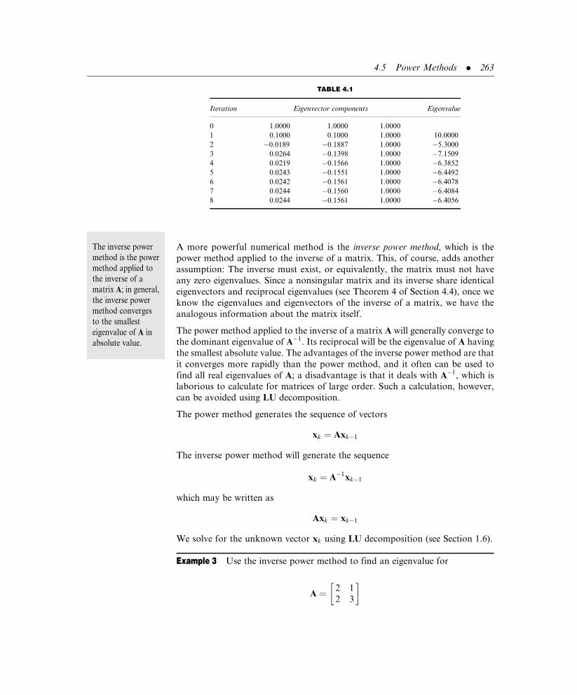
A more powerful numerical method is the inverse power method, which is the
power method applied to the inverse of a matrix. This, of course, adds another
assumption: The inverse must exist, or equivalently, the matrix must not have
any zero eigenvalues. Since a nonsingular matrix and its inverse share identical
eigenvectors and reciprocal eigenvalues (see Theorem 4 of Section 4.4), once we
know the eigenvalues and eigenvectors of the inverse of a matrix, we have the
analogous information about the matrix itself.
The power method applied to the inverse of a matrix A will generally converge to
the dominant eigenvalue of A�1. Its reciprocal will be the eigenvalue of A having
the smallest absolute value. The advantages of the inverse power method are that
it converges more rapidly than the power method, and it often can be used to
find all real eigenvalues of A; a disadvantage is that it deals with A�1, which is
laborious to calculate for matrices of large order. Such a calculation, however,
can be avoided using LU decomposition.
The power method generates the sequence of vectors
xk ¼ Axk�1
The inverse power method will generate the sequence
xk ¼ A�1xk�1
which may be written as
Axk ¼ xk�1
We solve for the unknown vector xk using LU decomposition (see Section 1.6).
Example 3 Use the inverse power method to find an eigenvalue for
A ¼ 2 1
2 3
� �
The inverse power
method is the power
method applied to
the inverse of a
matrix A; in general,
the inverse power
method converges
to the smallest
eigenvalue of A in
absolute value.
TABLE 4.1
Iteration Eigenvector components Eigenvalue
0 1.0000 1.0000 1.0000
1 0.1000 0.1000 1.0000 10.0000
2 �0.0189 �0.1887 1.0000 �5.3000
3 0.0264 �0.1398 1.0000 �7.1509
4 0.0219 �0.1566 1.0000 �6.3852
5 0.0243 �0.1551 1.0000 �6.4492
6 0.0242 �0.1561 1.0000 �6.4078
7 0.0244 �0.1560 1.0000 �6.4084
8 0.0244 �0.1561 1.0000 �6.4056
4.5 Power Methods . 263

Solution: We initialize x0 ¼ 1 1½ �T. The LU decomposition for A has A ¼ LU
with
L ¼ 1 0
1 1
� �and U ¼ 2 1
0 2
� �
For the first iteration, we solve the system LUx1 ¼ x0 by first solving the system
Ly ¼ x0 for y, and then solving the system Ux1 ¼ y for x1. Set y ¼ y1 y2½ �T and
x1 ¼ a b½ �T. The first system is
y1 þ 0y2 ¼ 1
y1 þ y2 ¼ 1
which has as its solution y1 ¼ 1 and y2 ¼ 0. The system Ux1 ¼ y becomes
2aþ b ¼ 1
2b ¼ 0
which admits the solution a ¼ 0:5 and b ¼ 0. Thus,
x1 ¼ A�1x0 ¼ 0:5 0½ �T
l � 0:5 (an approximation to an eigenvalue for A�1)
x1 1
0:50:5 0½ �T¼ 1 0½ �T
For the second iteration, we solve the system LUx2 ¼ x1 by first solving the
system Ly ¼ x1 for y, and then solving the system Ux2 ¼ y for x2. Set
y ¼ y1 y2½ �T and x2 ¼ a b½ �T. The first system is
y1 þ 0y2 ¼ 1
y1 þ y2 ¼ 0
which has as its solution y1 ¼ 1 and y2 ¼ �1. The system Ux2 ¼ y becomes
2aþ b ¼ 1
2b ¼ �1
which admits the solution a ¼ 0:75 and b ¼ �0:5. Thus,
x2 ¼ A�1x1 ¼ 0:75 �0:5½ �T
l � 0:75
x2 1
0:750:75 �0:5½ �T¼ 1 �0:666667½ �T
264 . Eigenvalues, Eigenvectors, and Differential Equations

For the third iteration, we first solve Ly ¼ x2 to obtain y ¼ 1 �1:666667½ �T,
and then Ux3 ¼ y to obtain x3 ¼ 0:916667 �0:833333½ �T Then,
l � 0:916667
x3 1
0:9166670:916667 �0:833333½ �T¼ 1 �0:909091½ �T
Continuing, we converge to the eigenvalue 1 for A�1 and its reciprocal 1=1 ¼ 1
for A. The vector approximations are converging to 1 �1½ �T , which is an eigen-
vector for both A�1 and A. &
Example 4 Use the inverse power method to find an eigenvalue for
A ¼7 2 0
2 1 6
0 6 7
24
35
Solution: We initialize x0 ¼ 1 1 1½ �T. The LU decomposition for A has
A ¼ LU with
L ¼
1 0 0
0:285714 1 0
0 14 1
2664
3775 and U ¼
7 2 0
0 0:428571 6
0 0 �77
2664
3775
For the first iteration, set y ¼ y1 y2 y3½ �T and x1 ¼ a b c½ �T. The first
system is
y1 þ 0y2 þ 0y3 ¼ 1
0:285714y1 þ y2 þ 0y3 ¼ 1
0y1 þ 14y2 þ y3 ¼ 1
which has as its solution y1 ¼ 1, y2 ¼ 0:714286, and y3 ¼ �9. The system
Ux1 ¼ y becomes
7aþ 2b ¼ 1
0:428571bþ 6c ¼ 0:714286
�77c ¼ �9
which admits the solution a ¼ 0:134199, b ¼ 0:030303, and c ¼ 0:116883. Thus,
4.5 Power Methods . 265
x1 ¼ A�1x0 ¼ 0:134199 0:030303 0:116833½ �T
l � 0:134199 (an approximation to an eigenvalue for A�1)
x1 1
0:1341990:134199 0:030303 0:116833½ �T
¼ 1 0:225806 0:870968½ �T
For the second iteration, solving the system Ly ¼ x1 for y, we obtain
y ¼ 1 �0:059908 1:709677½ �T
Then, solving the system Ux2 ¼ y for x2, we get
x2 ¼ 0:093981 0:171065 �0:022204½ �T
Therefore,
l � 0:171065
x2 1
0:1710650:093981 0:171065 �0:022204½ �T
¼ 0:549388 1 �0:129796½ �T
For the third iteration, solving the system Ly ¼ x2 for y, we obtain
y ¼ 0:549388 0:843032 �11:932245½ �T
Then, solving the system Ux3 ¼ y for x3, we get
x3 ¼ 0:136319 �0:202424 0:154964½ �T
Therefore,
l � �0:202424
x3 1
�0:2024240:136319 �0:202424 0:154964½ �T
¼ �0:673434 1 �0:765542½ �T
Continuing in this manner, we generate Table 4.2, where all entries are rounded
to four decimal places. The algorithm is converging to the eigenvalue �1=3 for
A�1 and its reciprocal �3 for A. The vector approximations are converging to
�0:2 1 �0:6½ �T, which is an eigenvector for both A�1 and A. &
266 . Eigenvalues, Eigenvectors, and Differential Equations

We can use Theorem 9 of Section 4.2 in conjunction with the inverse power
method to develop a procedure for finding all eigenvalues and a set of corre-
sponding eigenvectors for a matrix, providing that the eigenvalues are real and
distinct, and estimates of their locations are known. The algorithm is known as
the shifted inverse power method.
If c is an estimate for an eigenvalue of A, then A� cI will have an eigenvalue near
0 and its reciprocal will be the dominant eigenvalue of (A� cI)�1. We use the
inverse power method with an LU decomposition of A� cI to calculate the
dominant eigenvalue l and its corresponding eigenvector x for (A� cI)�1.
Then 1=l and x are an eigenvalue and eigenvector pair for A� cI while
cþ (1=l) and x are an eigenvalue and eigenvector pair for A.
TABLE 4.2
Iteration Eigenvector components Eigenvalue
0 1.0000 1.0000 1.0000
1 1.0000 0.2258 0.8710 0.1342
2 0.5494 1.0000 �0.1298 0.1711
3 �0.6734 1.0000 �0.7655 �0.2024
4 �0.0404 1.0000 �0.5782 �0.3921
5 �0.2677 1.0000 �0.5988 �0.3197
6 �0.1723 1.0000 �0.6035 �0.3372
7 �0.2116 1.0000 �0.5977 �0.3323
8 �0.1951 1.0000 �0.6012 �0.3336
9 �0.2021 1.0000 �0.5994 �0.3333
10 �0.1991 1.0000 �0.6003 �0.3334
11 �0.2004 1.0000 �0.5999 �0.3333
12 �0.1998 1.0000 �0.6001 �0.3333
The Shifted Inverse Power Method
Step 1. Begin with an initial guess x0 for an eigenvector of a matrix A,
having the property that the largest component of x0 in absolute
value is one. Set a counter k equal to 1 and choose a value for the
constant c (preferably an estimate for an eigenvalue if such an
estimate is available).
Step 2. Calculate xk ¼ (A� cI)�1xk�1.
Step 3. Set l equal to the largest component of xk in absolute value.
Step 4. Rescale xk by dividing each of its components by l. Relabel the
resulting vector as xk.
Step 5. If cþ (1=l) is an adequate estimate for an eigenvalue of A, with xk
as a corresponding eigenvector, stop; otherwise increment k by
one and return to Step 2.
4.5 Power Methods . 267

Example 5 Find a second eigenvalue for the matrix given in Example 4.
Solution: Since we do not have an estimate for any of the eigenvalues, we
arbitrarily choose c ¼ 15. Then
A� cI ¼
�8 2 0
2 �14 6
0 6 �8
26664
37775
which has an LU decomposition with
L ¼
1 0 0
�0:25 1 0
0 �0:444444 1
26664
37775 and U ¼
�8 2 0
0 �13:5 6
0 0 �5:333333
26664
37775
Applying the inverse power method to A� 15I, we generate Table 4.3, which is
converging to l ¼ �0:25 and x ¼ 1
3
2
31
� �T
. The corresponding eigenvalue of
A is (1=� 0:25)þ 15 ¼ 11, with the same eigenvector.
Using the results of Examples 4 and 5, we have two eigenvalues, l1 ¼ �3 and
l2 ¼ 11, of the 3� 3 matrix defined in Example 4. Since the trace of a matrix
equals the sum of the eigenvalues (Theorem 1 of Section 4.2), we know
7þ 1þ 7 ¼ �3þ 11þ l3, so the last eigenvalue is l3 ¼ 7. &
TABLE 4.3
Iteration Eigenvector components Eigenvalue
0 1.0000 1.0000 1.0000
1 0.6190 0.7619 1.0000 �0.2917
2 0.4687 0.7018 1.0000 �0.2639
3 0.3995 0.6816 1.0000 �0.2557
4 0.3661 0.6736 1.0000 �0.2526
5 0.3496 0.6700 1.0000 �0.2513
6 0.3415 0.6683 1.0000 �0.2506
7 0.3374 0.6675 1.0000 �0.2503
8 0.3354 0.6671 1.0000 �0.2502
9 0.3343 0.6669 1.0000 �0.2501
10 0.3338 0.6668 1.0000 �0.2500
11 0.3336 0.6667 1.0000 �0.2500
268 . Eigenvalues, Eigenvectors, and Differential Equations

Problems 4.5
In Problems 1 through 10, use the power method to locate the dominant eigenvalue and
a corresponding eigenvector for the given matrices. Stop after five iterations.
(1)2 1
2 3
� �. (2)
2 3
4 6
� �. (3)
3 6
9 6
� �.
(4)0 1
�4 6
� �. (5)
8 2
3 3
� �. (6)
8 3
3 2
� �.
(7)
3 0 0
2 6 4
2 3 5
24
35. (8)
7 2 0
2 1 6
0 6 7
24
35. (9)
3 2 3
2 6 6
3 6 11
24
35.
(10)
2 �17 7
�17 �4 1
7 1 �14
24
35.
(11) Use the power method on
A ¼2 0 �1
2 2 2
�1 0 2
24
35
and explain why it does not converge to the dominant eigenvalue l ¼ 3.
(12) Use the power method on
A ¼ 3 5
5 �3
� �
and explain why it does not converge.
(13) Shifting can also be used with the power method to locate the next most dominant
eigenvalue, if it is real and distinct, once the dominant eigenvalue has been deter-
mined. Construct A� lI, where l is the dominant eigenvalue of A, and apply the
power method to the shifted matrix. If the algorithm converges to m and x, then
mþ l is an eigenvalue of A with the corresponding eigenvector x. Apply this shifted
power method algorithm to the matrix in Problem 1. Use the result of Problem 1 to
determine the appropriate shift.
(14) Use the shifted power method as described in Problem 13 on the matrix in Problem
9. Use the results of Problem 9 to determine the appropriate shift.
(15) Use the inverse power method on the matrix defined in Example 1. Stop after five
iterations.
(16) Use the inverse power method on the matrix defined in Problem 3. Take
x0 ¼ [ 1 �0:5 ]T and stop after five iterations.
(17) Use the inverse power method on the matrix defined in Problem 5. Stop after five
iterations.
(18) Use the inverse power method on the matrix defined in Problem 6. Stop after five
iterations.
4.5 Power Methods . 269
(19) Use the inverse power method on the matrix defined in Problem 9. Stop after five
iterations.
(20) Use the inverse power method on the matrix defined in Problem 10. Stop after five
iterations.
(21) Use the inverse power method on the matrix defined in Problem 11. Stop after five
iterations.
(22) Use the inverse power method on the matrix defined in Problem 4. Explain the
difficulty and suggest a way to avoid it.
(23) Use the inverse power method on the matrix defined in Problem 2. Explain the
difficulty and suggest a way to avoid it.
(24) Can the power method converge to a dominant eigenvalue if that eigenvalue is not
distinct?
(25) Apply the shifted inverse power method to the matrix defined in Problem 9, with a
shift constant of 10.
(26) Apply the shifted inverse power method to the matrix defined in Problem 10, with a
shift constant of �25.
4.6 DIFFERENTIAL EQUATIONS IN FUNDAMENTAL FORM
An important application of Jordan canonical forms (see Appendix B), in
general, and the exponential of a matrix, in particular, occurs in the solution of
differential equations with constant coefficients. A working knowledge of the
integral calculus and a familiarity with differential equations is required to
understand the scope of this application. In this section, we show how to
transform many systems of differential equations into a matrix differential
equation. In the next section, we show how to solve such systems using the
exponential of matrix.
A differential equation in the unknown functions x1(t), x2(t), . . . , xn(t) is an
equation that involves these functions and one or more of their derivatives. We
shall be interested in systems of first order differential equations of the form
dx1(t)
dt¼ a11x1(t)þ a12x2(t)þ . . .þ a1nxn(t)þ f1(t)
dx2(t)
dt¼ a21x1(t)þ a22x2(t)þ . . .þ a2nxn(t)þ f2(t) (4:28)
..
.
dxn(t)
dt¼ a11x1(t)þ a12x2(t)þ . . .þ a1nxn(t)þ f1(t)
Here aij (i, j ¼ 1, 2, . . . , n) is restricted to be a constant and fi(t) is presumed to be
a known function of the variable t. If we define
270 . Eigenvalues, Eigenvectors, and Differential Equations

x(t) ¼
x1(t)
x2(t)
..
.
xn(t)
26664
37775, A ¼
a11 a12 . . . a1n
a21 a22 . . . a2n
..
. ... . .
. ...
an1 an2 . . . ann
26664
37775, and f(t) ¼
f1(t)
f2(t)
..
.
fn(t)
26664
37775 (4:29)
then equation (4.28) is equivalent to the single matrix equation
dx(t)
dt¼ Ax(t)þ f(t) (4:30)
Example 1 The system of equations
dx(t)
dt¼ 2x(t)þ 3y(t)þ 4z(t)þ (t2 � 1)
dy(t)
dt¼ 5y(t)þ 6z(t)þ et
dz(t)
dt¼ 7x(t)� 8y(t)� 9z(t)
is equivalent to the matrix equation
dx(t)=dt
dy(t)=dt
dz(t)=dt
264
375 ¼ 2 3 4
0 5 6
7 �8 �9
24
35 x(t)
y(t)
z(t)
24
35þ t2 � 1
et
0
24
35
This matrix equation is in form (4.30) with
x(t) ¼x(t)
y(t)
z(t)
24
35, A ¼
2 3 4
0 5 6
7 �8 �9
24
35, and f(t) ¼
t2 � 1
et
0
264
375
In this example, x1(t) ¼ x(t), x2(t) ¼ y(t), and x3(t) ¼ z(t). &
We solve equation (4.30) in the interval a � t � b by identifying a column matrix
x(t) that when substituted into (4.30) makes the equation true for all values of t in
the given interval. Often, however, we need to solve more than just a set of
differential equations. Often, we seek functions x1(t), x2(t), . . . , xn(t) that satisfy
all the differential equations in (4.28) or, equivalently, equation (4.30) and also
a set of initial conditions of the form
x1(t0) ¼ c1, x2(t0) ¼ c2, . . . , xn(t0) ¼ c0 (4:31)
where c1, c2, . . . , cn are all constants, and t0 is a specific value of the variable
t inside the interval of interest. Upon defining
4.6 Differential Equations in Fundamental Form . 271

c ¼
c1
c2
..
.
cn
26664
37775
it follows that
x(t0) ¼
x1(t0)
x2(t0)
..
.
xn(t0)
26664
37775 ¼
c1
c2
..
.
cn
26664
37775 ¼ c
Thus, initial conditions (4.31) have the matrix form
x(t0) ¼ c (4:32)
We say that a system of differential equations is in fundamental form if it is given
by the matrix equations
dx(t)
dt¼ Ax(t)þ f(t)
x(t0) ¼ c
(4:33)
Example 2 The system of equations
dr(t)
dt¼ 2r(t)� 3s(t)
ds(t)
dt¼ 4r(t)þ 5s(t)
r(p) ¼ 10, s(p) ¼ �20
is equivalent to the matrix equations
dr(t)=dt
ds(t)=dt
" #¼
2 �3
4 5
� �r(t)
s(t)
� �þ
0
0
� �
r(p)
s(p)
� �¼
10
�20
� �
This set of equations is in fundamental form (4.33) with
x(t) ¼ r(t)
s(t)
� �, A ¼ 2 �3
4 5
� �, f(t) ¼ 0
0
� �, and c ¼ 10
�20
� �
In this example, x1(t) ¼ r(t) and x2(t) ¼ s(t). &
A system of
differential
equations is in
fundamental form if
it is given by the
matrix equations
dx(t)
dt¼ Ax(t)þ f(t)
x(t0) ¼ c:
272 . Eigenvalues, Eigenvectors, and Differential Equations

A system of differential equations in fundamental form is homogeneous when
f(t) ¼ 0 and nonhomogeneous when f(t) 6¼ 0 (that is, when at least one element of
f(t) is not zero). The system in Example 2 is homogeneous; the system in Example
1 is nonhomogeneous.
Generally, systems of differential equations do not appear in fundamental form.
However, many such systems can be transformed into fundamental form by
appropriate reduction techniques. One such group are initial-value problems of
the form
an
dnx(t)
dtnþan�1
dn�1x(t)
dtn�1þ . . .þ a1
dx(t)
dtþ a0x(t) ¼ f (t)
x(t0) ¼ c1,dx(t0)
dt¼ c2, . . . ,
dn�1x(t0)
dtn�1¼ cn�1
(4:34)
This is a system containing a single nth-order, linear differential equation with
constant coefficients along with n� 1 initial conditions at t0. The coefficients
a0, a1, . . . , an are restricted to be constants and the function f(t) is presumed to be
known and continuous on some interval centered around t0.
A method of reduction for transforming system (4.34) into fundamental form is
given by the following six steps.
Step 1. Solve system (4.34) for the nth derivative of x(t).
dnx(t)
dtn¼ � an�1
an
dn�1x(t)
dtn�1� . . .� a1
an
dx(t)
dt� a0
an
x(t)þ f (t)
an
Step 2. Define n new variables (the same number as the order of the differential
equations) x1(t),x2(t), . . . , xn(t) by the equations
x1 ¼ x(t), x2 ¼dx
dt, x3 ¼
d2x
dt2, . . . , xn�1 ¼
dn�2x
dtn�2, xn ¼
dn�1x
dtn�1
(4:35)
Here we simplified xj(t) ( j ¼ 1, 2, . . . , n) to xj. By differentiating the
last equation in system (4.35), we obtain
dxn
dt¼ dnx
dtn(4:36)
Step 3. Substitute equations (4.35) and (4.36) into the equation obtained in
Step 1, thereby obtaining an equation for dxn=dt in terms of the new
variables. The result is
dxn
dt¼ � an�1
an
xn � . . .� a1
an
x2 �
a0
an
x1 þ
f (t)
an
(4:37)
A system of
differential
equations in
fundamental form is
homogeneous when
f(t) ¼ 0.
4.6 Differential Equations in Fundamental Form . 273

Step 4. Using (4.35) and (4.37), construct a system of n first-order differential
equations for x1, x2, . . . , xn. The system is
dx1
dt¼ x2
dx2
dt¼ x3
..
.
dxn�1
dt¼ xn
dxn
dt¼ � a0
an
x1 �
a1
an
x2 � . . .� an�1
an
xn þ
f (t)
an
(4:38)
In this last equation, the order of the terms in equation (4.37) was
rearranged so that x1 appears before x2, which appears before x3 and
so on. This was done to simplify the next step.
Step 5. Write system (4.38) as a single matrix differential equation. Define
x(t) ¼
x1
x2
..
.
xn�1
xn
26666666664
37777777775, f(t) ¼
0
0
..
.
0
f (t)=an
26666666664
37777777775
A ¼
0 1 0 0 . . . 0
0 0 1 0 . . . 0
0 0 0 1 . . . 0
..
. ... ..
. ... ..
.
0 0 0 0 . . . 1
� a0
an
� a1
an
� a2
an
� a3
an
. . . � an�1
an
266666666666664
377777777777775
Then equation (4.38) is equivalent to the matrix equationdx(t)
dt¼
Ax(t)þ f(t).
Step 6. Write the initial conditions as a matrix equation. Define
c ¼ c1 c2 . . . cn½ �T. Then,
274 . Eigenvalues, Eigenvectors, and Differential Equations

x(t0) ¼
x1(t0)
x2(t0)
..
.
xn(t0)
26664
37775 ¼
x(t0)
dx(t0)=dt
..
.
dn�1x(t0)=dtn�1
266664
377775 ¼
c1
c2
..
.
cn
26664
37775 ¼ c
The results of Steps 5 and 6 are a matrix system in fundamental form. &
Example 3 Write the initial-value problem
d2x(t)
dt2þ x(t) ¼ 2; x(p) ¼ 0,
dx(p)
dt¼ �1
in fundamental form.
Solution: The differential equation may be rewritten as
d2x(t)
dt2¼ �x(t)þ 2
This is a second-order differential equation, so we define two new variables
x1 ¼ x(t) and x2 ¼dx
dt. Thus,
dx2
dt¼ d2x
dt2and the original differential equation
becomesdx2
dt¼ �x1 þ 2. A first-order system for the new variables is
dx1
dt¼ x2 ¼ 0x1 þ 1x2
dx2
dt¼ �x1 þ 2 ¼ �1x1 þ 0x2 þ 2
Define x(t) ¼ x1
x2
� �, A ¼ 0 1
�1 0
� �, f(t) ¼ 0
2
� �, and c ¼ 0
�1
� �. Then, the
initial-value problem is equivalent to the fundamental form
dx(t)
dt¼ Ax(t)þ f(t); x(p) ¼ c &
Example 4 Write the initial-value problem
2d4x
dt4� 4
d3x
dt3þ 16
d2x
dt2� dx
dtþ 2x ¼ sin t
x(0) ¼ 1,dx(0)
dt¼ 2,
d2x(0)
dt2¼ �1,
d3x(0)
dt3¼ 0
in fundamental form.
4.6 Differential Equations in Fundamental Form . 275

Solution: The differential equation may be rewritten as
d4x
dt4¼ 2
d3x
dt3� 8
d2x
dt2þ 1
2
dx
dt� xþ 1
2sin t
This is a fourth-order differential equation, so we define four new variables
x1 ¼ x(t), x2 ¼dx
dt, x3 ¼
d2x
dt2, and x4 ¼
d3x
dt3
Thus,dx4
dt¼ d4x
dt4and the original differential equation becomes
dx4
dt¼ 2x4 � 8x3 þ
1
2x2 � x1 þ
1
2sin t
A first-order system for the new variables is
dx1
dt¼ x2
dx2
dt¼ x3
dx3
dt¼ x4
dx4
dt¼ �x1 þ
1
2x2 � 8x3 þ 2x4 þ
1
2sin t:
Define x(t) ¼
x1
x2
x3
x4
26664
37775, A ¼
0 1 0 0
0 0 1 0
0 0 0 1
�1 12�8 2
26664
37775, f(t) ¼
0
0
012
sin t
26664
37775, and
c ¼
1
2
�1
0
2664
3775.
Then, the initial-value problem is equivalent to the fundamental form
dx(t)
dt¼ Ax(t)þ f(t); x(0) ¼ c &
276 . Eigenvalues, Eigenvectors, and Differential Equations

Problems 4.6
Put the following initial-value problems into fundamental form:
(1)dx (t)
dt¼ 2x (t)þ 3y (t)
dy (t)
dt¼ 4x (t)þ 5y (t)
x (0) ¼ 6, y (0) ¼ 7
(2)dy (t)
dt¼ 3y (t)þ 2z (t)
dz (t)
dt¼ 4y (t)þ z (t)
y (0) ¼ 1, z (0) ¼ 1
(3)dx (t)
dt¼ �3x (t)þ 3y (t)þ 1
dy (t)
dt¼ 4x (t)� 4y (t)� 1
x (0) ¼ 0, y (0) ¼ 0
(4)dx (t)
dt¼ 3x (t)þ t
dy (t)
dt¼ 2x (t)þ tþ 1
x (0) ¼ 1, y (0) ¼ �1
(5)dx (t)
dt¼ 3x (t)þ 7y (t)þ 2
dy (t)
dt¼ x (t)þ y (t)þ 2t
x (1) ¼ 2, y (1) ¼ �3
(6)du (t)
dt¼ u (t)þ v (t)þ w (t)
dv (t)
dt¼ u (t)� 3v (t)þ w (t)
dw (t)
dt¼ v (t)þ w (t)
u (4) ¼ 0, v (4) ¼ 1,w (4) ¼ �1
(7)dx (t)
dt¼ 6y (t)þ z (t)
dy (t)
dt¼ x (t)� 3z (t)
dz (t)
dt¼ �2y (t)
x (0) ¼ 10, y (0) ¼ 10, z (0) ¼ 20
(8)dr (t)
dt¼ r (t)� 3s (t)� u (t)þ sin t
ds (t)
dt¼ r (t)� s (t)þ t2 þ 1
dt (t)
dt¼ 2r (t)þ s (t)� u (t)þ cos t
r (1) ¼ 4, s (1) ¼ �2, u (1) ¼ 5
(9)d2x (t)
dt2� 2
dx (t)
dt� 3x (t) ¼ 0
x (0) ¼ 4,dx (0)
dt¼ 5
(10)d2x (t)
dt2þ dx (t)
dt� x (t) ¼ 0
x (1) ¼ 2,dx (1)
dt¼ 0
(11)d2x (t)
dt2� x (t) ¼ t2
x (0) ¼ �3,dx (0)
dt¼ 3
(12)d2x (t)
dt2� 2
dx (t)
dt� 3x (t) ¼ 2
x (0) ¼ 0,dx (0)
dt¼ 0
(13)d2x (t)
dt2� 3
dx (t)
dtþ 2x (t) ¼ e�t
x (1) ¼ 2,dx (1)
dt¼ 2
(14)d3x (t)
dt3þ d2 (t)
dt2� x (t) ¼ 0
x (� 1) ¼ 2,dx (� 1)
dt¼ 1,
d2x (t)
dt2¼ �205
4.6 Differential Equations in Fundamental Form . 277

(15)d4x
dt4þ d2x
dt2¼ 1þ dx
dt
x(0) ¼ 1,dx(0)
dt¼ 2,
d2x(0)
dt2¼ p,
d3x(0)
dt3¼ e3
(16)d6x
dt6þ 4
d4x
dt4¼ t2 � t
x(p) ¼ 2,dx(p)
dt¼ 1,
d2x(p)
dt2¼ 0,
d3x(p)
dt3¼ 2
d4x(p)
dt4¼ 1,
d5x(p)
dt5¼ 0
4.7 SOLVING DIFFERENTIAL EQUATIONS IN FUNDAMENTAL FORM
We demonstrated in Section 4.6 how various systems of differential equations
could be transformed into the fundamental matrix form
dx(t)
dt¼ Ax(t)þ f(t)
x(t0) ¼ c
(4:39)
The matrix A is assumed to be a matrix of constants, as is the column matrix c. In
contrast, the column matrix f(t) may contain known functions of the variable t.
Such differential equations can be solved in terms of eAt.
The matrix differential equation in (4.39) can be rewritten as
dx(t)
dt� Ax(t) ¼ f(t)
If we premultiply each side of this equation by e�At, we obtain
e�At dx(t)
dt� Ax(t)
� �¼ e�Atf (t)
which may be rewritten as (see Corollary 1 of Section 4.4)
d
dte�Atx(t)� �
¼ e�Atf (t)
Integrating this last equation between the limits of t0 and t, we have
Z t
t0
d
dte�Atx(t)� �
dt ¼Z t
t0
e�Atf (t)dt
278 . Eigenvalues, Eigenvectors, and Differential Equations

or
e�Atx(t)
����t
t0
¼Z t
t0
e�Asf (s)ds (4:40)
Note that we have replaced the dummy variable t by the dummy variable s in the
right-side of equation (4.40), which has no effect on the definite integral (see
Problem 1). Evaluating the left side of equation (4.40), we obtain
e�Atx(t)� eAt0x(t0) ¼Z t
t0
e�Asf (s)ds
or
e�Atx(t) ¼ eAt0cþZ t
t0
e�Asf (s)ds (4:41)
where we substituted for x(t0) the initial condition x(t0) ¼ c. We solve explicitly
for x(t) by premultiplying both sides of equation (4.41) by (e�At)�1, whence
x(t) ¼ e�At� ��1
eAt0cþ e�At� ��1
Z t
t0
e�Asf (s)ds (4:42)
But (e�At)�1 ¼ eAt (see Theorem 2 of Section 4.4). Also, At commutes with At0,
so eAteAt0 ¼ eA(t�t0) (see Problem 36 of Section 4.4). Equation (4.42) may be
simplified to
x(t) ¼ eA(t�t0)cþ eAt
Z t
t0
e�Asf (s)ds (4:43)
and we have proven
" Theorem 1. The solution to the systemdx(t)
dt¼ Ax(t)þ f(t); x(t0) ¼ c
in fundamental form is
x(t) ¼ eA(t�t0)cþ eAt
Z t
t0
e�Asf (s)ds 3
A simple technique for calculating the matrices eA(t�t0) and e�As is to first find eAt
and then replace the variable t wherever it appears by the quantities (t� t0) and
(� s), respectively.
4.7 Solving Differential Equations in Fundamental Form . 279

Example 1 eAt ¼ e�t te�t
0 e�t
� �for A ¼ �1 1
0 �1
� �. Consequently,
eA(t�t0) ¼ e�(t�t0) (t� t0)e�(t�t0)
0 e�(t�t0)
� �and e�As ¼ es �ses
0 es
� �. &
Note that when t is replaced by (t� t0) in e�t, the result is e�(t�t0) ¼ e�tþt0 and not
e�t�t0 . That is, we replace the quantity t by the quantity (t� t0); we do not simply
add �t0 to the variable t wherever t appeared.
Example 2 Use matrix methods to solve
du(t)
dt¼ u(t)þ 2v(t)þ 1
dv(t)
dt¼ 4u(t)þ 3v(t)� 1
u(0) ¼ 1, v(0) ¼ 2
Solution: This system can be transformed into fundamental form if we define
x(t) ¼ u(t)
v(t)
� �, A ¼ 1 2
4 3
� �, f(t) ¼ 1
�1
� �, and c ¼ 1
2
� �
and take t0 ¼ 0. For this A, we calculate
eAt ¼ 1
6
2e5t þ 4e�t 2e5t � 2e�t
4e5t � 4e�t 4e5t þ 2e�t
� �
Hence,
e�As ¼ 1
6
2e�5s þ 4es 2e�5s � 2es
4e�5s � 4es 4e�5s þ 2es
� �
and
eAðt�t0Þ ¼ eAt
since t0 ¼ 0. Thus,
eAðt�t0Þc ¼ 1
6
2e5t þ 4e�t 2e5t � 2e�t
4e5t � 4e�t 4e5t þ 2e�t
" #1
2
� �
¼ 1
6
1½2e5t þ 4e�t� þ 2½2e5t � 2e�t�1½4e5t � 4e�t� þ 2½4e5t þ 2e�t�
" #
¼ e5t
2e5t
� �ð4:44Þ
280 . Eigenvalues, Eigenvectors, and Differential Equations

e�AsfðsÞ ¼ 1
6
2e�5s þ 4es 2e�5s � 2es
4e�5s � 4es 4e�5s þ 2es
" #1
�1
� �
¼ 1
6
1½2e�5s þ 4es� � 1½2e�5s � 2es�1½4e�5s � 4es� � 1½4e�5s þ 2es�
" #¼ es
�es
� �
Hence,
Z t
t0
e�AsfðsÞds ¼R t
0es dsR t
0�es ds
" #¼
esjt0�esjt0
" #¼
et � 1
�et þ 1
" #
eAt
Z t
t0
e�AsfðsÞ ds ¼ 1
6
2e5t þ 4e�t 2e5t � 2e�t
4e5t � 4e�t 4e5t þ 2e�t
" #ðet � 1Þð1� etÞ
" #
¼ 1
6
½2e5t þ 4e�t�½et � 1� þ ½2e5t � 2e�t�½1� et�
½4e5t � 4e�t�½et � 1� þ ½4e5t þ 2e�t�½1� et�
" #
¼ð1� e�tÞð�1þ e�tÞ
� �
ð4:45Þ
Substituting (4.44) and (4.45) into (4.43), we have
uðtÞvðtÞ
� �¼ xðtÞ ¼
e5t
2e5t
" #þ
1� e�t
�1þ e�t
� �¼
e5t þ 1� e�t
2e5t � 1þ e�t
" #
oruðtÞ ¼ e5t � e�t þ 1
vðtÞ ¼ 2e5t þ e�t � 1 &
Example 3 Use matrix methods to solve
d2y
dt2� 3
dy
dtþ 2y ¼ e�3t
y(1) ¼ 1,dy(1)
dt¼ 0
Solution: This system can be transformed into fundamental form if we define
x(t) ¼ x1(t)
x2(t)
� �, A ¼ 0 1
�2 3
� �, f(t) ¼
0
e�3t
� �, and c ¼ 1
0
� �
and take t0 ¼ 0. For this A, we calculate
4.7 Solving Differential Equations in Fundamental Form . 281

eAt ¼�e2t þ 2et e2t � et
�2e2t þ 2et 2e2t � et
" #
Thus,
eAðt�t0Þc ¼�e2ðt�1Þ þ 2eðt�1Þ e2ðt�1Þ � eðt�1Þ
�2e2ðt�1Þ þ 2eðt�1Þ 2e2ðt�1Þ � eðt�1Þ
" #1
0
� �
¼ �e2ðt�1Þ þ 2eðt�1Þ
�2e2ðt�1Þ þ 2eðt�1Þ
" #ð4:46Þ
Now
fðtÞ ¼0
e�3t
" #; fðsÞ ¼
0
e�3s
" #
e�AsfðsÞ ¼�e�2s þ 2e�s e�2s � e�s
�2e�2s þ 2e�s 2e�2s � e�s
" #0
e�3s
" #
¼e�5s � e�4s
2e�5s � e�4s
" #
Hence,
Z t
t0
e�AsfðsÞ ds ¼
R t
1ðe�5s � e�4sÞ ds
R 1
1ð2e�5s � e�4sÞ ds
264
375
¼ð� 1
5Þe�5t þ ð1
4Þe�4t þ ð1
5Þe�5 � ð1
4Þe�4
ð� 25Þe�5t þ ð1
4Þe�4t þ ð2
5Þe�5 � ð1
4Þe�4
24
35
eAt
Z t
t0
e�AsfðsÞ ds ¼ð�e2t þ 2etÞ ðe2t � etÞ
ð�2e2t þ 2etÞ ð2e2t � etÞ
" #
�� 1
5e�5t þ 1
4e�4t þ 1
5e�5 � 1
4e�4
� �� 2
5e�5t þ 1
4e�4t þ 2
5e�5 � 1
4e�4
� �24
35
¼120
e�3t þ 15eð2t�5Þ � 1
4et�4
� 320
e�3t þ 25eð2t�5Þ � 1
4et�4
24
35 ð4:47Þ
282 . Eigenvalues, Eigenvectors, and Differential Equations

Substituting (4.46) and (4.47) into (4.43), we have that
xðtÞ ¼x1ðtÞx2ðtÞ
" #¼
�e2ðt�1Þ þ 2et�1
�2e2ðt�1Þ þ 2et�1
" #þ
120
e�3t þ 15eð2t�5Þ � 1
4et�4
� 320
e�3t þ 25eð2t�5Þ � 1
4et�4
" #
¼�e2ðt�1Þ þ 2et�1 þ 1
20e�3t þ 1
5eð2t�5Þ � 1
4et�4
�2e2ðt�1Þ þ 2et�1 � 320
e�3t þ 25eð2t�5Þ � 1
4et�4
" #
It follows that the solution to the original initial-value problem is
y(t) ¼ x1(t) ¼ �e2(t�1) þ 2et�1 þ 1
20
e(2t�5) � 1
4et�4
&
The most tedious step in Example 3 was multiplying the matrix eAt by the column
matrixRtt0
e�Asf (s)ds. This step can be eliminated if we are willing to tolerate
a slightly more complicated integral. The integration in equation (4.43) is with
respect to the dummy variable s. If we bring the matrix eAt, appearing in front of
the integral, inside the integral, we may rewrite equation (4.43) as
x(t) ¼ eA(t�t0)cþZ t
t0
e�Ate�Asf (s) ds (4:48)
But At and �As commute, so eAte�As ¼ eA(t�s) and equation (4.48) becomes
x(t) ¼ eA(t�t0)cþZ t
t0
eA(t�s)f (s) ds (4:49)
The matrix eA(t�s) is obtained by replacing the variable t in eAt by the quantity
(t� s).
Example 4 Use matrix methods to solve
d2x
dt2þ x ¼ 2
x(p) ¼ 0,dx(p)
dt¼ �1
Solution: This system can be transformed into fundamental form if we define
x(t) ¼x1(t)
x2(t)
" #, A ¼
0 1
�1 0
" #, f(t) ¼
0
2
" #, and c ¼
0
�1
" #
An alternate form of
the solution to a
matrix differential
equation in
fundamental form is
x(t) ¼ eA(t�t0)c
þZ t
t0
eA(t�s)f (s) ds:
4.7 Solving Differential Equations in Fundamental Form . 283

and take t0 ¼ p. The solution to this initial-value problem is given by either
equation (4.43) or (4.49). In this example, we shall evaluate equation (4.49),
thereby saving one matrix multiplication. For this A, eAt was determined in
Example 8 of Section 4.4 to be
eAt ¼ cos t sin t
� sin t cos t
� �Thus,
eAðt�t0Þc ¼cosðt� pÞ sinðt� pÞ� sinðt� pÞ cosðt� pÞ
� �0
�1
� �
¼� sinðt� pÞ� cosðt� pÞ
� �
eAðt�sÞfðsÞ ¼cosðt� sÞ sinðt� sÞ� sinðt� sÞ cosðt� sÞ
� �0
2
� �
¼2 sinðt� sÞ2 cosðt� sÞ
� �
ð4:50Þ
Hence,
Z t
t0
eAðt�sÞfðsÞ ds ¼R t
p2 sinðt� sÞ dsR t
p2 cosðt� sÞ ds
" #
¼2� 2 cosðt� pÞ
2 sinðt� pÞ
� �ð4:51Þ
Substituting (4.50) and (4.51) into (4.49) and using the trigonometric identities
sinðt� pÞ ¼ � sin t and cosðt� pÞ ¼ � cos t, we have
x1ðtÞx2ðtÞ
� �¼ xðtÞ ¼
� sinðt� pÞ� cosðt� pÞ
� �þ
2� 2 cosðt� pÞ2 sinðt� pÞ
� �
¼sin tþ 2 cos tþ 2
cos t� 2 sin t
� �
Thus, since xðtÞ ¼ x1ðtÞ, it follows that the solution to the initial-value problem
is given by
xðtÞ ¼ sin tþ 2 cos tþ 2 &
A great simplification to both equation (4.43) and equation (4.49) is effected
when the differential equation is homogeneous, that is, when f(t) ¼ 0. In both
formulas, the integral becomes a zero-column matrix, and the solution reduces to
284 . Eigenvalues, Eigenvectors, and Differential Equations

x(t) ¼ eA(t�t0) c (4:52)
Occasionally, one needs to solve a differential equation by itself, and not an
entire initial-value problem. In such cases, the general solution is (see Problem 2)
x(t) ¼ eAtkþ eAt
Ze�Atf (t) dt (4:53)
where k is an arbitrary column matrix of suitable dimension. The general
solution to a homogeneous differential equation by itself is
x(t) ¼ eAtk (4:54)
Example 5 Use matrix methods to solve
du(t)
dt¼ u(t)þ 2v(t)
dv(t)
dt¼ 4u(t)þ 3v(t)
Solution: This system can be transformed into fundamental form if we define
x(t) ¼u(t)
v(t)
" #, A ¼
1 2
4 3
" #, and f(t) ¼
0
0
" #
This is a homogeneous system with no initial conditions specified; the general
solution is given in (4.54). For this A, we have
eAt ¼ 1
6
2e5t þ 4e�t 2e5t � 2e�t
4e5t � 4e�t 4e5t þ 2e�t
" #
Thus,
eAtk ¼ 1
6
2e5t þ 4e�t 2e5t � 2e�t
4e5t � 4e�t 4e5t þ 2e�t
" #k1
k2
" #
¼ 1
6
k1½2e5t þ 4e�t� þ k2½2e5t � 2e�t�
k1½4e5t � 4e�t� þ k2½4e5t þ 2e�t�
" #
¼ 1
6
e5tð2k1 þ 2k2Þ þ e�tð4k1 � 2k2Þ
e5tð4k1 þ 4k2Þ þ e�tð�4k1 þ 2k2Þ
" #ð4:55Þ
The solution to the
homogeneous
systemdx(t)
dt¼ Ax(t);
x(t0) ¼ c is
x(t) ¼ eA(t�t0)c.
4.7 Solving Differential Equations in Fundamental Form . 285

Substituting (4.55) into (4.54), we have that
uðtÞvðtÞ
" #¼ xðtÞ ¼ 1
6
e5tð2k1 þ 2k2Þ þ e�tð4k1 � 2k2Þ
e5tð4k1 þ 4k2Þ þ e�tð�4k1 þ 2k2Þ
" #
or
uðtÞ ¼ 2k1 þ 2k2
6
e5t þ 4k1 � 2k2
6
e�t
vðtÞ ¼ 22k1 þ 2k2
6
e5t þ �4k1 þ 2k2
6
e�t
ð4:56Þ
We can simplify the expressions for u(t) and v(t) if we introduce two new
arbitrary constants k3 and k4 defined by
k3 ¼2k1 þ 2k2
6; k4 ¼
4k1 � 2k2
6
Substituting these values into (4.56), we obtain
uðtÞ ¼ k3e5t þ k4e
�t
vðtÞ ¼ 2k3e5t � k4e
�t&
Problems 4.7
(1) Show by direct integration that
Z t
t0
t2dt ¼Z t
t0
s2ds ¼Z t
t0
p2dp
In general, show that if f(t) is integrable on the interval [a, b], then
Zb
a
f (t)dt ¼Zb
a
f (s)ds
Hint: AssumeR
f (t)dt ¼ F (t)þ c. Hence,R
f (s)ds ¼ F (s)þ c. Then use the funda-
mental theorem of integral calculus.
(2) Derive equation (4.53). Hint: Follow the derivation of equation (4.43) using
indefinite integration, rather than definite integration, and note thatZd
dte�Atx(t)� �
dt ¼ e�Atx(t)þ k
where k is an arbitrary column matrix of integration.
286 . Eigenvalues, Eigenvectors, and Differential Equations

(3) Find (a) e�At, (b) eAðt�2Þ, (c) eAðt�sÞ, (d) e�Aðt�2Þ, if
eAt ¼ e3t
1 t t2=2
0 1 t
0 0 1
264
375
(4) Find (a) e�At, (b) e�As, (c) eAðt�3Þ, if
eAt ¼ 1
6
2e5t þ 4e�t 2e5t � 2e�t
4e5t � 4e�t 4e5t þ 2e�t
" #
(5) Find (a) e�At, (b) e�As, (c) e�Aðt�sÞ, if
eAt ¼ 1
3
� sin 3tþ 3 cos 3t 5 sin 3t
�2 sin 3t sin 3tþ 3 cos 3t
" #
(6) Determine which of the following column vectors x are solutions to the system
d
dt
x1(t)
x2(t)
" #¼
0 1
�1 0
" #x1(t)
x2(t)
" #;
x1(0)
x2(0)
" #¼
1
0
" #
(a)sin t
cos t
� �, (b)
et
0
" #, (c)
cos t
� sin t
" #.
(7) Determine which of the following column vectors x are solutions to the system
d
dt
x1(t)
x2(t)
" #¼ 1 2
4 3
� �x1(t)
x2(t)
" #;
x1(0)
x2(0)
" #¼
1
2
" #
(a)e�t
�e�t
" #, (b)
e�t
2e�t
" #, (c)
e5t
2e5t
" #.
(8) Determine which of the following column vectors x are solutions to the system
d
dt
x1(t)
x2(t)
" #¼ 0 1
�2 3
� �x1(t)
x2(t)
" #;
x1(1)
x2(1)
" #¼
1
0
" #
(a)�e2t þ 2et
�2e2t þ 2et
" #, (b)
�e2(t�1) þ 2e(t�1)
�2e2(t�1) þ 2e(t�1)
" #, (c)
e2(t�1)
0
" #.
Solve the systems described in Problems 9 through 16 by matrix methods. Note that
Problems 9 through 12 have the same coefficient matrix.
4.7 Solving Differential Equations in Fundamental Form . 287

(9)dx(t)
dt¼ �2x(t)þ 3y(t)
dy(t)
dt¼ �x(t)þ 2y(t)
x(2) ¼ 2, y(2) ¼ 4
(10)dx(t)
dt¼ �2x(t)þ 3y(t)þ 1
dy(t)
dt¼ �x(t)þ 2y(t)þ 1
x(1) ¼ 1, y(1) ¼ 1
(11)dx(t)
dt¼ �2x(t)þ 3y(t)
dy(t)
dt¼ �x(t)þ 2y(t)
(12)dx(t)
dt¼ �2x(t)þ 3y(t)þ 1
dy(t)
dt¼ �x(t)þ 2y(t)þ 1
(13)d2 x
dt2þ 4x ¼ sin t; x(0) ¼ 1,
dx(0)
dt¼ 0
(14)d3 x
dt3¼ t; x(1) ¼ 1,
dx(1)
dt¼ 2,
d2 x(1)
dt2¼ 3
(15)d2 x
dt2� dx
dt� 2x ¼ e�t; x(0) ¼ 1,
dx(0)
dt¼ 0
(16)d2 x
dt2¼ 2
dx
dtþ 5yþ 3
dy
dt¼ � dx
dt� 2y
x(0) ¼ 0,dx(0)
dt¼ 0, y(0) ¼ 1:
4.8 A MODELING PROBLEM
Models are useful in everyday life. In this section, we will consider a mixing
problem. We will model the problem with a system of first order differential
equations. In our discussion, we will make various assumptions and observations
and then pose questions involving changes in various parameters.
Consider Figure 4.3. A saline solution, of concentration 2 pounds of salt per
gallon, is introduced into Tank 1 at a rate of 5 gallons per minute. As we can see
from the diagram, the tanks are connected by a system of pipes.
Assuming that the salt is distributed uniformly in the solution, we will model the
problem with the following variables:
t ¼ time (minutes)
S1(t) ¼ amount of salt in Tank 1 at time t (pounds)
S2(t) ¼ amount of salt in Tank 2 at time t (pounds)
S3(t) ¼ amount of salt in Tank 3 at time t (pounds)
dSk
dt¼ rate of change of salt in Tank k (pounds=minute), k ¼ 1, 2, 3
288 . Eigenvalues, Eigenvectors, and Differential Equations

Let us now consider Tank 1. Because there are three pipes connected to the tank,
the rate of change of the salt in this tank will have three terms:
dS1
dt¼ 5 gal
min� 2 lbs
gal� S1 lb
100 gal� 2 gal
min� S1 lb
100 gal� 3 gal
min(4:57)
We note in this equation the consistency of units (lbs/min) and the division by the
capacity of Tank 1 (100 gal).
The two other tanks are modeled as follows:
dS2
dt¼ S1 lb
100 gal� 2 gal
minþ S3 lb
100 gal� 4 gal
min� S2 lb
50 gal� 1 gal
min� S2 lb
50 gal� 5 gal
min(4:58)
dS3
dt¼ S2 lb
50 gal� 1 gal
min� S3 lb
100 gal� 4 gal
min� 0 lb
gal� 3 gal
min(4:59)
We note here that the last term of equation (4.59) is 0, because there is no salt in
the incoming solution from the right.
Finally, let us assume that initially there is no salt in any tank. That is,
S1(0) ¼ S2(0) ¼ S3(0) ¼ 0:
We now will rewrite our problem in matrix notation:
d
dt
S1
S2
S3
2664
3775 ¼
�5
1000 0
2
100
�6
50
4
100
01
50
�4
100
26666664
37777775
S1
S2
S3
2664
3775þ
10
0
0
2664
3775 (4:60)
We can now expand on the techniques discussed in Sections 4.6 and 4.7 to solve
this problem. However, in this case, the use of technological methods is preferred
(see Appendix E). This is primarily due to the fact that we have a 3-by-3
coefficient matrix instead of a 2-by-2 matrix.
Figure 4.3 Tank 1 Tank 2 Tank 32 gal/min 4 gal/min
5 gal/min
1 gal/min
5 gal/min
3 gal/min
2 lb/gal100gal
100gal
50gal
3 gal/min
4.8 A Modeling Problem . 289

We end our discussion with the following observations and ask the following
questions:
We note that the system was ‘‘closed’’; that is, the amount of solution coming
in (8 gal) is equal to the amount going out (8 gal). What if this was not the
case?
We assumed no salt was initially present. What if this was not the case?
If the salt in the solution was not uniformly distributed, the modeling of our
problem becomes much more difficult. The same is true if the solution is not
introduced continuously. In these cases, our approach must be radically
altered and a numerical approach might be more useful.
Problems 4.8
(1) Assume vat V1 is placed above vat V2 and that both vats have a capacity of 100 liters.
If 7 liters of a sucrose solution (5 kg sugar/liter) is poured into V1 every minute, how
much sugar is in each vat at time t, if V1 drains into V2 at the rate of 7 liters/minute,
while V2 drains off at the same rate and there is no sugar in either vat initially?
(2) Consider the previous problem. If vat V2 drains off at a rate of 8 liters/minute, how
much sugar will it contain in the long run, realizing that it will eventually be empty?
(3) Consider the previous problem. If vat V2 drains off at a rate of 6 liters/minute, how
much sugar will it contain in the long run, realizing that it will eventually overflow?
(4) Solve problem 1 if V1(0) ¼ 5 and V2(0) ¼ 12.
(5) Suppose two lakes (x and y) are connected by a series of canals in such a way that the
rate of change of the pollution in each lake can be modeled by the following matrix
equation:
d
dt
x
y
� �¼ �2 3
4 �3
� �x
y
� �þ 1
0
� �
where x(t) and y(t) represent the amount of pollution (in tons) at time t (months). If
both lakes are initially clean, find the amount of pollution at time t, along with the
long range pollution in each lake.
(6) Do the previous problem if the model is given by
d
dt
x
y
� �¼ �2 �3
�4 �3
� �x
y
� �þ 1
0
� �
(7) Suppose Problem 5 is modeled by
d
dt
x
y
� �¼ �2 �3
�4 �3
� �x
y
� �
with x(0) ¼ 100, and y(0) ¼ 300. Find the long-range pollution of each lake.
290 . Eigenvalues, Eigenvectors, and Differential Equations

Chapter 4 Review
Important Terms
Important Concepts
Section 4.1 " A nonzero vector x is an eigenvector of a square matrix A if there exists a scalar
l, called an eigenvalue, such that Ax ¼ lx.
" Similar matrices have the same characteristic equation (and, therefore, the same
eigenvalues).
" Nonzero vectors in the eigenspace of the matrix A for the eigenvalue l are
eigenvectors of A.
" Eigenvalues and eigenvectors for a linear transformation T: V! V are deter-
mined by locating the eigenvalues and eigenvectors of any matrix representation
for T; the eigenvectors of the matrix are coordinate representations of the
eigenvector of T.
Section 4.2 " Any nonzero scalar multiple of an eigenvector is again an eigenvector; the
nonzero sum of two eigenvectors corresponding to the same eigenvalue is again
an eigenvector
" The sum of the eigenvalues of a matrix equals the trace of the matrix.
" The eigenvalues of an upper (lower) triangular matrix are the elements on the
main diagonal of the matrix.
" The product of all the eigenvalues of a matrix (counting multiplicity) equals the
determinant of the matrix.
characteristic equation (p. 222)
determinant (p. 219)
derivative of a matrix (p. 256)
diagonalizable matrix (p. 238)
dominant eigenvalue (p. 259)
eAt (p. 253)
eigenspace (p. 225)
eigenvalue (p. 220)
eigenvector (p. 220)
Euler’s relations (p. 255)
exponential of a matrix (p. 251)
fundamental form of differential
equations (p. 272)
homogeneous differential
equation (p. 285)
initial conditions (p. 271)
inverse power method (p. 263)
modal matrix (p. 238)
model (p. 288)
nonhomogeneous differential
equation (p. 273)
power method (p. 259)
shifted inverse power
method (p. 267)
spectral matrix (p. 238)
trace (p. 232)
Chapter 4 Review . 291

" A matrix is singular if and only if it has a zero eigenvalue.
" If x is an eigenvector of A corresponding to the eigenvalue l, then
(i) for any nonzero scalar k, kl and x are a corresponding pair of eigenvalues
and eigenvectors of kA,
(ii) ln and x are a corresponding pair of eigenvalues and eigenvectors of An,
for any positive integer n,
(iii) for any scalar c, l� c and x are a corresponding pair of eigenvalues and
eigenvectors of A� cI,
(iv) 1=l and x are a corresponding pair of eigenvalues and eigenvectors of A�1,
providing the inverse exists,
(v) l is an eigenvalue of AT .
Section 4.3 " An n� n matrix is diagonalizable if and only if it has n linearly independent
eigenvectors.
" Eigenvectors of a matrix corresponding to distinct eigenvalues are linearly inde-
pendent.
" If l is an eigenvalue of multiplicity k of an n� n matrix A, then the number of
linearly independent eigenvectors of A associated with l is n� r(A� lI), where r
denotes rank.
" If V is an n-dimensional vector space, then a linear transformation T: V! V
may be represented by a diagonal matrix if and only if T possesses a basis of
eigenvectors.
Section 4.4 " To calculate the exponential of a diagonal matrix, replace each diagonal element
by the exponential of that diagonal element.
" If A is similar to a matrix J in Jordan canonical form, so that A ¼MJM�1 for a
generalized modal matrix M, then eA ¼MeJM�1.
" e0 ¼ I, where 0 is the n� n zero matrix and I is the n� n identity matrix.
Section 4.5 " The power method is a numerical method for estimating the dominant eigenvalue
and a corresponding eigenvector for a matrix.
" The inverse power method is the power method applied to the inverse of a matrix
A. In general, the inverse power method converges to the smallest eigenvalue in
absolute value of A.
Section 4.6 " A differential equation in the unknown functions x1(t),x2(t), . . . , xn(t) is an
equation that involves these functions and one or more of their derivatives.
292 . Eigenvalues, Eigenvectors, and Differential Equations

Section 4.7 " The solution to the systemdx(t)
dt¼ Ax(t)þ f(t); x(t0) ¼ c is
x(t) ¼ eA(t�t0)cþ eAt
Z t
t0
e�Asf(s)ds
¼ eA(t�t0)cþZ t
t0
e�A(t�s)f(s)ds
" The solution to the homogenous equationdx(t)
dt¼ Ax(t); x(t0) ¼ c is
x(t) ¼ eA(t�t0)c
Section 4.8 " Models are useful in everyday life.
Chapter 4 Review . 293

This page intentionally left blank

Chapter 5
Euclidean Inner Product
5.1 ORTHOGONALITY
Perpendicularity is such a useful concept in Euclidean geometry that we want to
extend the notion to all finite dimensional vector spaces. This is relatively easy
for vector spaces of two or three dimensions, because such vectors have graphical
representations. Each vector in a two-dimensional vector space can be written as
a 2-tuple and graphed as a directed line segment (arrow) in the plane. Similarly,
each vector in a three-dimensional vector space can be written as a 3-tuple and
graphed as a directed line segment in space. Using geometrical principles on such
graphs, we can determine whether directed line segments from the same vector
space meet at right angles. However, to extend the concept of perpendicularity to
Rn, n > 3, we need a different approach.
The Euclidean inner product of two column matrices x ¼ x1 x2 x3 . . . xn½ �T and
y ¼ y1 y2 y3 . . . yn½ �T in Rn, denoted by x, yh i, is
x, yh i ¼ x1y1 þ x2y2 þ x3y3 þ . . .þ xnyn (5:1)
To calculate the Euclidean inner product, we multiply corresponding compon-
ents of two column matrices in Rn and sum the resulting products. Although we
will work exclusively in this chapter with n-tuples written as column matrices, the
Euclidean inner product is equally applicable to row matrices. Either way, the
Euclidean inner product of two vectors in Rn is a real number and not another
vector in Rn. In terms of column matrices,
x, yh i ¼ xTy (5:2)
Example 1 The Euclidean inner product of x ¼1
2
3
2435 and y ¼
4
�5
6
24
35 in R3 is
x, yh i ¼ 1(4)þ 2(� 5)þ 3(6) ¼ 12
The inner product
of two vectors x and
y in Rn is a real
number determined
by multiplying
corresponding
components of x
and y and then
summing the
resulting products.
295

while the Euclidean inner product of u ¼
20
�4
30
10
2664
3775 and v ¼
10
�5
�8
�6
2664
3775 in R4 is
u, vh i ¼ 20(10) þ (� 4)(� 5)þ 30(� 8)þ 10(� 6) ¼ �80 &
" Theorem 1. If x, y, and z are vectors in Rn, then
(a) x, xh i is positive if x 6¼ 0; x, xh i ¼ 0 if and only if x ¼ 0.
(b) x, yh i ¼ y, xh i.(c) lx, yh i ¼ l x, yh i, for any real number l.
(d) xþ z, yh i ¼ x, yh i þ z, yh i.(e) 0, yh i ¼ 0: 3
Proof: We prove parts (a) and (b) here and leave the proofs of the other parts
as exercises (see Problems 28 through 30). With x ¼ x1 x2 x3 . . . xn½ �T,
we have
x, xh i ¼ (x1)2 þ (x2)
2 þ (x3)2 þ . . .þ (xn)
2
This sum of squares is zero if and only if x1 ¼ x2 ¼ x3 ¼ . . . ¼ xn ¼ 0, which in
turn implies that x ¼ 0. If any component is not zero, that is, if x is not the zero
vector in Rn, then the sum of the squares must be positive.
For part (b), we set y ¼ y1 y2 y3 . . . yn½ �T. Then
x, yh i ¼ x1y1 þ x2y2 þ x3y3 þ . . .þ xnyn
¼ y1x1 þ y2x2 þ y3x3 þ . . .þ ynxn
¼ y, xh i &
The magnitude of an n-tuple x (see Section 1.7) is related to the Euclidean inner
product by the formula
kxk ¼ffiffiffiffiffiffiffiffiffiffiffiffihx, xi
p¼
ffiffiffiffiffiffiffiffiffiffiffiffiffiffiffiffiffiffiffiffiffiffiffiffiffiffiffiffiffiffiffiffiffiffiffiffiffiffiffiffiffiffiffiffiffiffiffix2
1 þ x22 þ x2
3 þ . . .þ x2n
q: (5:3)
Example 2 The magnitude of x ¼ 2 �3 �4½ �T in R3 is
kxk ¼ffiffiffiffiffiffiffiffiffiffiffiffihx, xi
p¼
ffiffiffiffiffiffiffiffiffiffiffiffiffiffiffiffiffiffiffiffiffiffiffiffiffiffiffiffiffiffiffiffiffiffiffiffiffiffiffiffiffiffiffiffiffiffi(2)2 þ (� 3)2 þ (� 4)2
q¼
ffiffiffiffiffi29p
while the magnitude of y ¼ 1 �1 1 �1½ �T in R4 is
kyk ¼ffiffiffiffiffiffiffiffiffiffiffihy, yi
p¼
ffiffiffiffiffiffiffiffiffiffiffiffiffiffiffiffiffiffiffiffiffiffiffiffiffiffiffiffiffiffiffiffiffiffiffiffiffiffiffiffiffiffiffiffiffiffiffiffiffiffiffiffiffiffiffiffiffiffiffiffi(1)2 þ (� 1)2 þ (1)2 þ (� 1)2
q¼ 2 &
The magnitude of
a vector x in Rn is
the square root of
the inner product
of x with itself.
296 . Euclidean Inner Product

A unit vector is a vector having a magnitude of 1. A nonzero vector x is
normalized if it is divided by its magnitude. It follows that
1
kxk x,1
kxk x� �
¼ 1
kxk x,1
kxk x
� �Part (c) of Theorem 1
¼ 1
kxk1
kxk x, x
� �Part (b) of Theorem 1
¼ 1
kxk
� �2
hx, xi Part (c) of Theorem 1
¼ 1
kxk
� �2
kxk2
(5.3)
¼ 1
Thus, a normalized vector is always a unit vector.
As with other vector operations, the Euclidean inner product has a geometrical
interpretation in two or three dimensions. For simplicity, we consider two-
dimensional vectors here; the extension to three dimensions is straightforward.
Let u and v be two nonzero vectors in R2 represented by directed line segments in
the plane, each emanating from the origin. The angle between u and v is the angle
u between the two line segments, with 0� � u � 180� as illustrated in Figure 5.1.
The vectors u and v, along with their difference u� v, form a triangle (see
Figure 5.2) having sides kuk, kvk, and ku� vk. It follows from the law of cosines
that
ku� vk2 ¼ kuk2 þ kvk2 � 2kukkvk cos u
Figure 5.1
θ
u
v
5.1 Orthogonality . 297

where upon
kukkvk cos � ¼ 12kuk2 þ kvk2 � ku� vk2� �
¼ 12
u, uh i þ v, vh i � u� v, u� vh ið Þ
¼ 12
u, uh i þ v, vh i � [ u, uh i � 2 u, vh i þ v, vh i]ð Þ
¼ u, vh i (5:4)
and
cos u ¼ u, vh ikukkvk (5:5)
Weuse equation (5.5) to calculate the angle between twodirected line segments in R2.
Example 3 Find the angle between the vectors u ¼ 2
5
� and v ¼ �3
4
� .
Solution:
u, vh i ¼ 2(� 3)þ 5(4) ¼ 14, kuk ¼ffiffiffiffiffiffiffiffiffiffiffiffiffiffi4þ 25p
¼ffiffiffiffiffi29p
, kvk ¼ffiffiffiffiffiffiffiffiffiffiffiffiffiffi9þ 16p
¼ 5;
so cos u ¼ 14
5ffiffiffiffiffi29p � 0:5199; and u � 58:7�: &
If u is a nonzero vector in R2, we have from Theorem 1 that u, uh i is positive and
then, from equation (5.3), that kuk > 0. Similarly, if v is a nonzero vector in R2,
then kvk > 0. Because
u, vh i ¼ kukkvk cos u, (5:4 repeated)
we see that the inner product of two nonzero vectors in R2 is 0 if and only if
cos u ¼ 0. The angle u is the angle between the two directed line segments
representing u and v (see Figure 5.1) with 0� � u � 180�. Thus, cos u ¼ 0 if and
only if u ¼ 90�, from which we conclude that the inner product of two nonzero
Figure 5.2
θ
u
v
u − v
Two vectors in the
same vector space
are orthogonal if
their Euclidean
inner product is
zero.
298 . Euclidean Inner Product
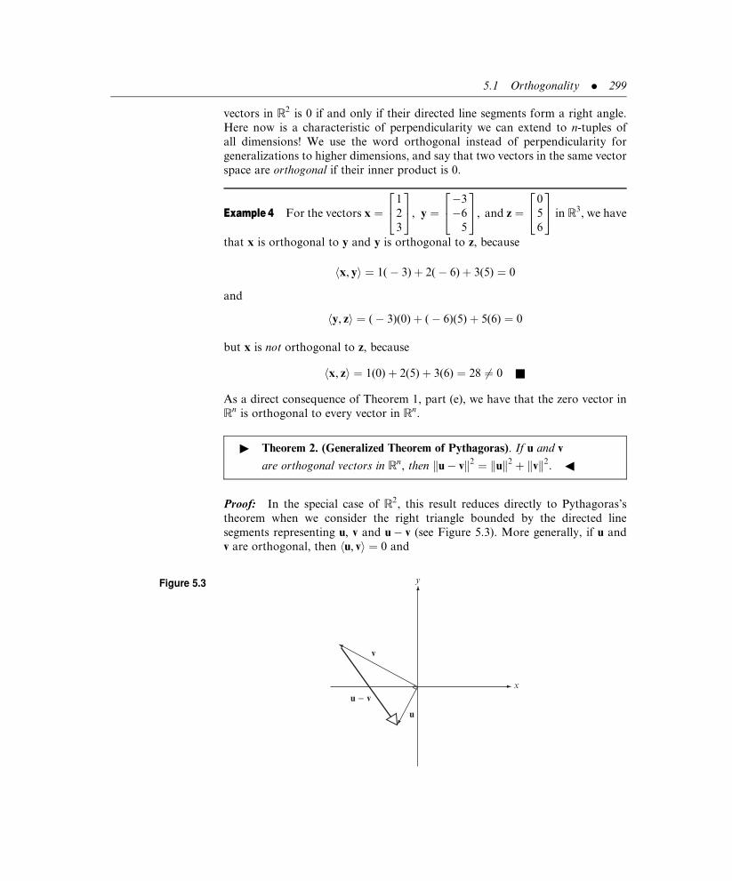
vectors in R2 is 0 if and only if their directed line segments form a right angle.
Here now is a characteristic of perpendicularity we can extend to n-tuples of
all dimensions! We use the word orthogonal instead of perpendicularity for
generalizations to higher dimensions, and say that two vectors in the same vector
space are orthogonal if their inner product is 0.
Example 4 For the vectors x ¼1
2
3
2435, y ¼
�3
�6
5
24
35, and z ¼
0
5
6
2435 in R3, we have
that x is orthogonal to y and y is orthogonal to z, because
x, yh i ¼ 1(� 3)þ 2(� 6)þ 3(5) ¼ 0
and
y, zh i ¼ (� 3)(0)þ (� 6)(5)þ 5(6) ¼ 0
but x is not orthogonal to z, because
x, zh i ¼ 1(0)þ 2(5)þ 3(6) ¼ 28 6¼ 0 &
As a direct consequence of Theorem 1, part (e), we have that the zero vector in
Rn is orthogonal to every vector in Rn.
" Theorem 2. (Generalized Theorem of Pythagoras). If u and v
are orthogonal vectors in Rn, then ku� vk2 ¼ kuk2 þ kvk2. 3
Proof: In the special case of R2, this result reduces directly to Pythagoras’s
theorem when we consider the right triangle bounded by the directed line
segments representing u, v and u� v (see Figure 5.3). More generally, if u and
v are orthogonal, then u, vh i ¼ 0 and
Figure 5.3
u
v
y
xu − v
5.1 Orthogonality . 299

ku� vk2 ¼ u� v, u� vh i¼ u, uh i � 2 u, vh i þ v, vh i¼ u, uh i � 2(0)þ v, vh i¼ kuk2 þ kvk2 &
" Theorem 3. (Cauchy-Schwarz Inequality). If u and v are vectors in Rn,
then j u, vh ij � kukkvk: 3
Proof: In the special case of R2, we have
u, vh i ¼ kukkvk cos u, (5:4 repeated)
hence
j u, vh ij ¼ kukkvk cos uj j¼ jkukkvjj cos uj� kukkvk
because j cos uj � 1 for any angle u. The proof for more general vector spaces is
left as an exercise (see Problems 35 and 36). &
The Euclidean inner product in Rn induces an inner product on pairs of vectors
in other n-dimensional vector spaces. A vector in an n-dimensional vector space
V has a coordinate representation with respect to a underlying basis (see Section
2.4). We define an inner product on two vectors x and y in V by forming the
Euclidean inner product on the coordinate representations of both vectors with
respect to the same underlying basis.
Example 5 Calculate A, Bh i for A ¼ 4 3
6 2
� and B ¼ 1 2
1 2
� in the vector
space M2�2 with respect to the standard basis
S ¼ 1 0
0 0
� ,
0 1
0 0
� ,
0 0
1 0
� ,
0 0
0 1
� �
Solution: The coordinate representations with respect to this basis are
4 3
6 2
� $
4
3
6
2
26643775 and
1 2
1 2
� $
1
2
1
2
26643775
The induced inner product is
A, Bh i ¼ 4(1)þ 3(2)þ 6(1)þ 2(2) ¼ 20
An induced inner
product on two
matrices of the same
order is obtained by
multiplying
corresponding
elements of both
matrices and
summing the results.
300 . Euclidean Inner Product

With respect to the standard basis, the induced inner product of two matrices of
the same order is obtained by multiplying corresponding elements of both matri-
ces and summing the results. &
Example 6 Redo Example 5 with respect to the basis
B ¼ 0 1
1 1
� ,
1 0
1 1
� ,
1 1
0 1
� ,
1 1
1 0
� �
Solution: The coordinate representations with respect to this basis is (see
Example 13 of Section 2.4)
x ¼ 4 3
6 2
� $
1
2
�1
3
2664
3775
B
and y ¼ 1 2
1 2
� $
1
0
1
0
26643775
B
The induced inner product is now
A, Bh i ¼ 1(1)þ 2(0)þ (� 1)(1)þ 3(0) ¼ 0
which is different from the inner product calculated in Example 5. &
It follows from the previous two examples that an inner product depends on the
underlying basis; different bases can induce different inner products. Consequently,
two vectors can be orthogonal with respect to one basis, as in Example 6, and
notorthogonal with respect to another basis, as in Example 5. We can see this
distinction graphically, by considering the vectors
x ¼ 1
1
� and y ¼ 1
�1
�
With respect to the standard basis
S ¼ e1 ¼1
0
� , e2 ¼
0
1
� �
x, yh i ¼ 0, and x is perpendicular to y, as illustrated in Figure 5.4.
If, instead, we take as the basis
D ¼ d1 ¼2
1
� , d2 ¼
5
2
� �
then we have as coordinate representations in the D basis,
An inner product is
basis dependent.
Two vectors can be
orthogonal with
respect to one basis
and not orthogonal
with respect to
another basis.
5.1 Orthogonality . 301

x ¼1
1
� ¼ (3)
2
1
� þ (� 1)
5
2
� $
3
�1
� D
y ¼1
�1
� ¼ (� 7)
2
1
� þ (3)
5
2
� $�7
3
� D
d1 ¼2
1
� ¼ (1)
2
1
� þ (0)
5
2
� $
1
0
� D
d2 ¼5
2
� ¼ (0)
2
1
� þ (1)
5
2
� $
0
1
� D
Graphing the coordinate representations in the D basis, we generate
Figure 5.5. Note that x and y are no longer perpendicular. Indeed,
Figure 5.4 y
x
y
2
1
1 2
−1
−1−2
−2
xe2 e1
Figure 5.5
−1 1 2 3 4−2−3−4−5−6−7−8
4
3
2
1
−1
−2
−3
−4
y
x
x
y
θ
d2d1
302 . Euclidean Inner Product

x, yh i ¼ 3(� 7)þ (� 1)(3) ¼ 24 6¼ 0. Furthermore, x, xh i ¼ (3)2 þ (� 1)2 ¼ 10,
y, yh i ¼ (� 7)2 þ (3)2 ¼ 58, and it follows from equation (5.5) that the angle
between x and y is
u ¼ arccos�24ffiffiffiffiffi10p ffiffiffiffiffi
58p � 175�
Example 7 Calculate p(t); q(t)h i with respect to the standard basis in P2 for
p(t) ¼ 3t2 � tþ 5 and q(t) ¼ �2t2 þ 4tþ 2
Solution: Using the standard basis S ¼ ft2, t, 1g, we have the coordinate
representations
3t2 � tþ 5$3
�1
5
24
35 and � 2t2 þ 4tþ 2$
�2
4
2
24
35
The induced inner product is
p(t); q(t)h i ¼ 3(� 2)þ (� 1)(4)þ 5(2) ¼ 0
and the polynomials are orthogonal. With respect to the standard basis, the
induced inner product of two polynomials is obtained by multiplying the coef-
ficients of like powers of the variable and summing the results. &
Problems 5.1
In Problems 1 through 17, (a) find x, yh i, (b) find jxj, and (c) determine whether x and y
are orthogonal.
(1) x ¼ 1 2½ �T, y ¼ 3 4½ �T.
(2) x ¼ 1 1½ �T, y ¼ �4 4½ �T.
(3) x ¼ �5 7½ �T, y ¼ 3 �5½ �T.
(4) x ¼ �2 �8½ �T, y ¼ 20 �5½ �T.
(5) x ¼ �3 4½ �T, y ¼ 0 0½ �T.
(6) x ¼ 2 0 1½ �T, y ¼ 1 2 4½ �T.
(7) x ¼ �2 2 �4½ �T, y ¼ �4 3 �3½ �T.
(8) x ¼ �3 �2 5½ �T, y ¼ 6 �4 �4½ �T.
(9) x ¼ 10 20 30½ �T, y ¼ 5 �7 3½ �T.
(10) x ¼ 14
12
18
� T, y ¼ 1
313
13
� T.
An induced inner
product of two
polynomials is
obtained by
multiplying the
coefficients of like
powers of the
variable and
summing the results.
5.1 Orthogonality . 303

(11) x ¼ 1 0 1 1½ �T, y ¼ 1 1 0 1½ �T.
(12) x ¼ 1 0 1 �1½ �T, y ¼ 1 1 0 1½ �T.
(13) x ¼ 1 0 1 0½ �T, y ¼ 0 1 0 1½ �T.
(14) x ¼ 12
12
12
12
� T, y ¼ 1 2 3 �4½ �T.
(15) x ¼ 12
12
0 12
� T, y ¼ 1
312
1 �23
� T.
(16) x ¼ 1 2 3 4 5½ �T, y ¼ 1 2 �3 4 �5½ �T.
(17) x ¼ 1 2 3 4 5 6½ �T, y ¼ 1 2 3 4 5½ �T.
(18) Normalize the following vectors:
(a) y as defined in Problem 1.
(b) y as defined in Problem 4.
(c) y as defined in Problem 6.
(d) y as defined in Problem 7.
(e) y as defined in Problem 10.
(f) y as defined in Problem 17.
In Problems 19 through 26, find the angle between the given vectors.
(19) x ¼ 1 2½ �T, y ¼ 2 1½ �T.
(20) x ¼ 1 1½ �T, y ¼ 3 5½ �T.
(21) x ¼ 3 �2½ �T, y ¼ 3 3½ �T.
(22) x ¼ 4 �1½ �T, y ¼ 2 8½ �T.
(23) x ¼ �7 �2½ �T, y ¼ 2 9½ �T.
(24) x ¼ 2 1 0½ �T, y ¼ 2 0 2½ �T.
(25) x ¼ 1 1 0½ �T, y ¼ 2 2 1½ �T.
(26) x ¼ 0 3 4½ �T, y ¼ 2 5 5½ �T.
(27) Find x if x, ah ib ¼ c when a ¼ 1 3 �1½ �T, b ¼ 2 1 1½ �T and
c ¼ 3 0 �1½ �T.
(28) Prove that if x and y are vectors in Rn, then lx, yh i ¼ l x, yh i for any real number l.
(29) Prove that if x, y and z are vectors in Rn, then xþ z, yh i ¼ x, yh i þ z, yh i.
(30) Prove for any vector y in Rn that 0, yh i ¼ 0.
(31) Prove that if x and y are orthogonal vectors in Rn, then kxþ yk2 ¼ kxk2 þ kyk2.
(32) Prove the parallelogram law for any two vectors x and y in Rn:
kxþ yk2 þ kx� yk2 ¼ 2kxk2 þ 2kyk2:
304 . Euclidean Inner Product

(33) Prove that for any two vectors x and y in Rn:
kxþ yk2 � kx� yk2 ¼ 4 x, yh i:
(34) Let x, y and z be vectors in Rn. Show that if x is orthogonal to y and if x is orthogonal
to z then x is also orthogonal to all linear combinations of the vectors x and y.
(35) Prove that, for any scalar l,
0 � klx� yk2 ¼ l2kxk2 � 2l x, yh i þ kyk2:
(36) (Problem 35 continued) Take l ¼ x, yh i=kxk2 and show that
0 � �hx, yi2
kxk2þ kyk2
From this deduce that
x, yh i2� kxk2kyk2
and then the Cauchy-Schwarz inequality.
(37) Prove that the Cauchy-Schwarz inequality is an equality in R2 if and only if one
vector is a scalar multiple of the other.
(38) Use the Cauchy-Schwarz inequality to show that
�1 � hu, vikukkvk � 1:
Thus, equation (5.5) can be used to define the cosine of the angle between
any two vectors in Rn. Use equation (5.5) to find the cosine of the angle
between the following x and y vectors
(a) x ¼ 0 1 1 1½ �T, y ¼ 1 1 1 0½ �T,
(b) x ¼ 1 2 3 4½ �T, y ¼ 1 �2 0 �1½ �T,
(c) x ¼ 12
12
12
12
� T, y ¼ �1 �1 �1 �1½ �T,
(d) x ¼ 1 1 2 2 3½ �T, y ¼ 1 2 3 2 1½ �T,
(e) x ¼ 1 2 3 4 5 6½ �T, y ¼ 1 1 1 1 1 1½ �T.
(39) Verify the following relationships:
kxþ yk2 ¼ kxk2 þ 2 x, yh i þ kyk2
� kxk2 þ 2kxkkyk þ kyk2
¼ (kxk þ kyk)2
and then deduce the triangle inequality
kxþ yk � kxk þ kyk
5.1 Orthogonality . 305

(40) Calculate induced inner products for the following pairs of matrices with respect to
standard bases:
(a) A ¼ 1 5
6 2
� and B ¼ 5 5
1 4
� in M2�2,
(b) A ¼ 1 �2
0 4
� and B ¼ 3 �3
2 �8
� in M2�2,
(c) A ¼ �2 7
1 1
� and B ¼ 2 �3
2 6
� in M2�2,
(d) A ¼4 2
1 �3
3 �5
24
35 and B ¼
1 2
3 4
5 6
24
35 in M3�2,
(e) A ¼ 1 2 3
4 5 6
� and B ¼ 1 1 2
�3 2 �3
� in M2�3,
(f) A ¼1 2 3
4 5 6
7 8 9
24
35 and B ¼
�3 4 1
2 0 �4
5 1 2
24
35 in M3�3.
(41) Redo parts (a), (b), and (c) of Problem 40 with respect to the basis
C ¼ 1 1
0 0
� ,
1 �1
0 0
� ,
0 0
1 1
� ,
0 0
1 �1
� �:
(42) A generalization of the inner product for n-dimensional column matrices with real
components is
x, yh iA¼ Ax, Ayh i
where the inner product on the right is the Euclidean inner product between Ax and
Ay for a given n� n real, nonsingular matrix A. Show that x, yh iA satisfies all the
properties of Theorem 1.
(43) Calculate x, yh iA for the vectors in Problem 1 when A ¼ 2 3
1 �1
� :
(44) Calculate x, yh iA for the vectors in Problem 6 when A ¼1 1 0
1 0 1
0 1 1
24
35.
(45) Redo Problem 44 with A ¼1 �1 1
0 1 �1
1 1 1
24
35.
(46) Show that x, yh iA is the Euclidean inner product when x and y are coordinate
representations with respect to a basis B made up of the columns of A and A is the
transition matrix from the B basis to the standard basis.
(47) Calculate induced inner products for the following pairs of polynomials with
respect to standard bases:
306 . Euclidean Inner Product

(a) p (t) ¼ t2 þ 2tþ 3 and q (t) ¼ t2 þ 3t� 5 in P2,
(b) p (t) ¼ 10t2 � 5tþ 1 and q (t) ¼ 2t2 � t� 30 in P2,
(c) p (t) ¼ t2 þ 5 and q (t) ¼ 2t2 � 2tþ 1 in P2,
(d) p (t) ¼ 2t2 þ 3t and q (t) ¼ tþ 8 in P2,
(e) p (t) ¼ 3t3 þ 2t2 � tþ 4 and q (t) ¼ t3 þ t in P3,
(f) p (t) ¼ t3 � t2 þ 2t and q (t) ¼ t2 þ tþ 1 in P3.
(48) Redo parts (a) through (d) of Problem 47 with respect to the basis
B ¼ f t2, tþ 1, t g:
(49) A different inner product on P n is defined by
p (t); q (t)h i ¼Zb
a
p (t) q (t) dt
for polynomials p(t) and q(t) and real numbers a and b with b > a. Show
that this inner product satisfies all the properties of Theorem 1.
(50) Redo Problem 47 with the inner product defined in Problem 48, taking a ¼ 0
and b ¼ 1.
5.2 PROJECTIONS
An important problem in the applied sciences is to write a given nonzero vector x
in R2 or R3 as the sum of two vectors uþ v where u is parallel to a known
reference vector a and v is perpendicular to a (see Figure 5.6). In physics, u is
called the parallel component of x and v is called the perpendicular component of
x, where parallel and perpendicular are relative to the reference vector a.
If u is to be parallel to a, it must be a scalar multiple of a; that is, u ¼ la for some
value of the scalar l. If x ¼ uþ v, then necessarily v ¼ x� u ¼ x� la. If u and
v are to be perpendicular, then
0 ¼ u, vh i ¼ la, x� lah i¼ l a, xh i � l2 a, ah i¼ l½ a, xh i � l a, ah i�
Either l ¼ 0 or l ¼ a, xh i= a, ah i. If l ¼ 0, then u ¼ la ¼ 0a ¼ 0, and
x ¼ uþ v ¼ v, from which we conclude that x and a, the given vector and the
reference vector, are perpendicular and a, xh i ¼ 0. Thus, l ¼ a, xh i= a, ah i is
always true and
5.2 Projections . 307

u ¼ ha, xiha, ai a and v ¼ x� ha, xi
ha, ai a
In this context, u is the projection of x onto a and v is the orthogonal complement.
Example 1 Write the vector x ¼ 2
7
� as the sum of two vectors, one parallel to
a ¼ �3
4
� and one perpendicular to a.
Solution:
a, xh i ¼ �3(2)þ 4(7) ¼ 22
a, ah i ¼ (� 3)2 þ (4)2 ¼ 25,
¼ ha, xiha, ai a ¼ 22
25
�3
4
24
35 ¼ �2:64
3:52
24
35
v ¼ x� u ¼2
7
2435� �2:64
3:52
24
35 ¼ 4:64
3:48
24
35
Then, x ¼ uþ v, with u parallel to a and v perpendicular to a. &
Example 2 Find the point on the line xþ 4y ¼ 0 closest to (� 3, � 1).
Solution: One point on the line is (4, � 1), so a ¼ 4 �1½ �T is a reference vector
in the plane parallel to the line. The given point (� 3, � 1) is associated with the
vector x ¼ �3 �1½ �T, and we seek the coordinates of the point P (see Figure 5.7)
on the line xþ 4y ¼ 0. The vector u that begins at the origin and terminates at P is
the projection of x onto a. Therefore,
Figure 5.6
u
xv a
308 . Euclidean Inner Product

a, xh i ¼ 4(� 3)þ (� 1)(� 1) ¼ �11
a, ah i ¼ (4)2 þ (� 1)2 ¼ 17
u ¼ ha, xiha, ai a ¼
�11
17
4
�1
" #¼�44=17
11=17
" #
P ¼ (� 44=17, 11=17) &
The concepts of projections and orthogonal complements in R2 can be extended
to any finite dimensional vector space V with an inner product. Given a nonzero
vector x and a reference vector a, both in V, we define the projections of x onto
a as
projax ¼ha, xiha, ai a (5:6)
It then follows (see Problem 34) that
x� ha, xiha, ai a is orthogonal to a (5:7)
Subtracting from a nonzero vector x the projection x onto another nonzero
vector a leaves a vector that is orthogonal to both a and the projection of x
onto a. &
Example 3 Write the polynomial x(t) ¼ 2t2 þ 3tþ 4 in P2 as the sum of two
polynomials, one that is the projection of x(t) onto a(t) ¼ 5t2 þ 6 and one that is
orthogonal to a(t) under the inner product induced by the Euclidean inner
product in R3.
Figure 5.7
−1 2 3 4−2x
v
−3−4−5
4
3
2
1
−1
−2
−3
−4
y
x
a1
Pu
Line: x + 4y = 0
(−3, −1) (4, −1)
Subtracting from a
nonzero vector x its
projection onto
another nonzero
vector a yields a
vector that is
orthogonal to both
a and the projection
of x onto a.
5.2 Projections . 309

Solution: The induced inner product between two polynomials is obtained by
multiplying the coefficients of like powers of t and summing the resulting
products (see Example 7 of Section 5.1). Thus,
a(t), x(t)h i ¼ 5(2)þ 0(3)þ 6(4) ¼ 34
a(t), a(t)h i ¼ (5)2 þ (0)2 þ (6)2 ¼ 61
u(t) ¼ ha(t), x(t)iha(t), a(t)i a(t) ¼ 34
61(5t2 þ 6) ¼ 170
61t2 þ 204
61
is the projection of x(t) onto a(t).
v(t) ¼ x(t)� u(t) ¼ � 48
61t2 þ 3tþ 40
61
is orthogonal to a(t), and x(t) ¼ u(t)þ v(t). &
A set of vectors is called an orthogonal set if each vector in the set is orthogonal
to every other vector in the set.
Example 4 The vectors x, y, zf g in R3 defined by
x ¼1
1
1
2435, y ¼
1
1
�2
24
35, z ¼
1
�1
0
24
35
are an orthogonal set of vectors because x, yh i ¼ x, zh i ¼ y, zh i ¼ 0. In contrast,
the set of vectors fa, b, cg in R4 defined by
a ¼ 1 1 0 1½ �T, b ¼ �1 1 2 0½ �T, c ¼ 1 1 0 2½ �T
is not an orthogonal set because a, ch i 6¼ 0. If c is redefined as
c ¼ 1 1 0 �2½ �T
then fa, b, cg is orthogonal, because now a, bh i ¼ a, ch i ¼ b, ch i ¼ 0. &
An orthogonal set of unit vectors (vectors all having magnitude 1) is called an
orthonormal set. Using the Kronecker delta notation,
dij ¼1 if i ¼ j
0 if i 6¼ j
(5:8)
We say that a set of vectors x1, x2, . . . , xnf g is orthonormal if and only if
xi, xj
� �¼ dij (i, j ¼ 1, 2, . . . , m) (5:9)
An orthonormal set
of vectors is an
orthogonal set of
unit vectors.
310 . Euclidean Inner Product

Example 5 The set of vectors fu, v, wg in R3 defined by
u ¼1=
ffiffiffi2p
1=ffiffiffi2p
0
2664
3775, v ¼
1=ffiffiffi2p
�1=ffiffiffi2p
0
2664
3775, w ¼
0
0
1
26643775
is an orthonormal set of vectors because each vector is orthogonal to the other
two and each vector is a unit vector. &
Any orthogonal set of nonzero vectors can be transformed into an orthonormal
set by dividing each vector by its magnitude. It follows from Example 4 that the
vectors
x ¼1
1
1
2435, y ¼
1
1
�2
24
35, z ¼
1
�1
0
24
35
form an orthogonal set. Dividing each vector by its magnitude, we generate
x
kxk ,y
kyk ,z
kzk
�¼
1=ffiffiffi3p
1=ffiffiffi3p
1=ffiffiffi3p
24
35,
1=ffiffiffi6p
1=ffiffiffi6p
�2=ffiffiffi6p
24
35,
1=ffiffiffi2p
�1=ffiffiffi2p
0
24
35
8<:
9=;
as an orthonormal set.
" Theorem 1. An orthonormal set of a finite number of vectors is linearly
independent. 3
Proof: Let fx1, x2, . . . , xng be an orthonormal set and consider the vector equation
c1x1 þ c2x2 þ . . .þ cnxn ¼ 0 (5:10)
where cj ( j ¼ 1, 2, . . . , n) is a scalar. This set of vectors is linearly independent if
and only if the only solution to equation (5.10) is c1 ¼ c2 ¼ . . . ¼ cn ¼ 0. Taking
the inner product of both sides of equation (5.10) with xj, we have
c1x1 þ c2x2 þ . . .þ cjxj þ . . .þ cnxn, xj
� �¼ 0, xj
� �Usingparts (c), (d), and (e)ofTheorem1ofSection5.1,we rewrite this last equationas
c1 x1, xj
� �þ c2 x2, xj
� �þ . . .þ cj xj , xj
� �þ . . .þ cn xn, xj
� �¼ 0
or
Xn
i¼1
cihxi, xji ¼ 0
5.2 Projections . 311

As a consequence of equation (5.9),
Xn
i¼1
cidij ¼ 0
or cj ¼ 0 ( j ¼ 1, 2, . . . , n): &
If B ¼ fx1, x2, . . . , xng is a basis for V, then any vector x in V can be written as a
linear combination of the basis vectors in one and only one way (see Theorem 5
of Section 2.4). That is,
x ¼ c1x1 þ c2x2 þ . . .þ cnxn ¼Xn
i¼1
cixi
with each ci (i ¼ 1, 2, . . . , n) uniquely determined by the choice of the basis. If the
basis is orthonormal, we can use the additional structure of an inner product to
say more. In particular,
hx, xji ¼Xn
i¼1
cixi, xj
* +
¼Xn
i¼1
hcixi, xji
¼Xn
i¼1
cihxi, xji
¼Xn
i¼1
cidij ¼ cj:
We have proven Theorem 2.
" Theorem 2. If fx1, x2, . . . , xng is orthonormal basis for a vector space V,
then for any vector x in V,
x ¼ x, x1h ix1 þ x, x2h ix2 þ . . .þ x, xnh ixn: 3
Theorem 2 is one of those wonderful results that saves time and effort. In
general, to write a vector in an n-dimensional vector space in terms of a given
basis, we must solve a set n simultaneous linear equations (see Examples 12 and
13 of Section 2.4). If, however, the basis is orthonormal, the work is reduced to
taking n-inner products and solving no simultaneous equations.
Example 6 Write x ¼ 1 2 3½ �T as a linear combination of the vectors
q1 ¼1=
ffiffiffi3p
1=ffiffiffi3p
1=ffiffiffi3p
264
375, q2 ¼
1=ffiffiffi6p
1=ffiffiffi6p
�2=ffiffiffi6p
264
375, q3 ¼
1=ffiffiffi2p
�1=ffiffiffi2p
0
264
375
312 . Euclidean Inner Product

Proof: The set fq1, q2, q3g is an orthonormal basis for R3. Consequently,
hx, q1i ¼ 11ffiffiffi3p� �
þ 21ffiffiffi3p� �
þ 31ffiffiffi3p� �
¼ 6ffiffiffi3p
hx, q2i ¼ 11ffiffiffi6p� �
þ 21ffiffiffi6p� �
þ 3 � 2ffiffiffi6p
� �¼ �3ffiffiffi
6p
hx, q3i ¼ 11ffiffiffi2p� �
þ 2�1ffiffiffi
2p� �
þ 3(0) ¼ �1ffiffiffi2p
1
2
3
26643775 ¼ 6ffiffiffi
3p
1=ffiffiffi3p
1=ffiffiffi3p
1=ffiffiffi3p
2664
3775þ �3ffiffiffi
6p� � 1=
ffiffiffi6p
1=ffiffiffi6p
�2=ffiffiffi6p
2664
3775þ �1ffiffiffi
2p� � 1=
ffiffiffi2p
�1=ffiffiffi2p
0
2664
3775 &
Example 7 Write A ¼ 1 2
3 4
� as a linear combination of the four matrices
Q1 ¼1=
ffiffiffi3p
1=ffiffiffi3p
�1=ffiffiffi3p
0
24
35,
Q2 ¼0 �1=
ffiffiffi3p
�1=ffiffiffi3p
1=ffiffiffi3p
24
35,
Q3 ¼1=
ffiffiffi3p
0
1=ffiffiffi3p
1=ffiffiffi3p
24
35,
Q4 ¼�1=
ffiffiffi3p
1=ffiffiffi3p
0 1=ffiffiffi3p
24
35
Solution: The set fQ1, Q2, Q3, Q4g is an orthonormal basis for M2�2 under the
induced inner product (see Example 5 of Section 5.1) defined by multiplying
corresponding elements and summing the resulting products. Consequently,
hA, Q1i ¼1 2
3 4
� ,
1=ffiffiffi3p
1=ffiffiffi3p
�1=ffiffiffi3p
0
" #* +
¼ 11ffiffiffi3p� �
þ 21ffiffiffi3p� �
þ 3�1ffiffiffi
3p� �
þ 4(0) ¼ 0
5.2 Projections . 313

hA, Q2i ¼*
1 2
3 4
" #,
0 �1=ffiffiffi3p
�1=ffiffiffi3p
1=ffiffiffi3p
" #+
¼ 1(0)þ 2�1ffiffiffi
3p� �
þ 3�1ffiffiffi
3p� �
þ 41ffiffiffi3p� �
¼ �1ffiffiffi3p
hA, Q3i ¼*
1 2
3 4
" #,
1=ffiffiffi3p
0
1=ffiffiffi3p
1=ffiffiffi3p
" #+
¼ 11ffiffiffi3p� �
þ 2(0)þ 31ffiffiffi3p� �
þ 41ffiffiffi3p� �
¼ 8ffiffiffi3p
hA, Q4i ¼*
1 2
3 4
" #,�1=
ffiffiffi3p
1=ffiffiffi3p
0 1=ffiffiffi3p
" #+
¼ 1�1ffiffiffi
3p� �
þ 21ffiffiffi3p� �
þ 3(0)þ 41ffiffiffi3p� �
¼ 5ffiffiffi3p
and
1 2
3 4
" #¼ (0)
1=ffiffiffi3p
1=ffiffiffi3p
�1=ffiffiffi3p
0
" #þ �1ffiffiffi
3p� � 0 �1=
ffiffiffi3p
�1=ffiffiffi3p
1=ffiffiffi3p
" #
þ 8ffiffiffi3p� � 1=
ffiffiffi3p
0
1=ffiffiffi3p
1=ffiffiffi3p
" #þ 5ffiffiffi
3p� � �1=
ffiffiffi3p
1=ffiffiffi3p
0 1=ffiffiffi3p
" #: &
An inner product space is a vector space with an inner product defined between
pairs of vectors. Using projections, we can transform any basis for a finite
dimensional inner product space V into an orthonormal basis for V. To see
how, let fx1, x2, x3g be a basis for R3. Taking x1 as our reference vector, it
follows from equation (5.7), with x2 replacing x, that
x4 ¼ x2 �hx1, x2ihx1, x1i
x1 is orthogonal to x1:
Similarly, it follows from equation (5.7), with x3 replacing x, that
x5 ¼ x3 �hx1, x3ihx1, x1i
x1 is orthogonal to x1
These formulas may be simplified when x1 is a unit vector, because
x1, x1h i ¼ kx1k2 ¼ 1. We can guarantee that the first vector in any basis be a
An inner product
space is a vector
space with an inner
product defined
between pairs of
vectors.
314 . Euclidean Inner Product
unit vector by dividing that vector by its magnitude. Assuming this has been
done and noting that x1, x2h i ¼ x2, x1h i and x1, x3h i ¼ x3, x1h i, we have that
x4 ¼ x2 � hx2, x1ix1 is orthogonal to x1
and
x5 ¼ x3 � hx3, x1ix1 is orthogonal to x1
Furthermore, x4 6¼ 0 because it is a linear combination of x1 and x2, which are
linearly independent, with the coefficient of x2 equal to 1. The only way for
a linear combination of linearly independent vectors to be 0 is for all the
coefficients of the vectors to be 0. Similarly x5 6¼ 0 because it is a linear combin-
ation of x1 and x3 with the coefficient of x3 set to 1. Thus, the set fx1, x4, x5g has
the property that x1 is a unit vector orthogonal to both nonzero vectors x4 and
x5. The vectors x4 and x5 are not necessarily unit vectors and may not be
orthogonal, but we have made progress in our attempt to create an orthonormal
set. Now, taking x4 as our reference vector, it follows from equation (5.7), with
x5 replacing x, that
x6 ¼ x5 �hx4, x5ihx4, x4i
x4 is orthogonal to x4
This formula may be simplified if x4 is a unit vector, a condition we can force by
dividing x4 by its magnitude. Assuming this has been done and noting that
x4, x5h i ¼ x5, x4h i, we have that
x6 ¼ x5 � hx5, x4ix4 is orthogonal to x4
Also,
hx6, x1i ¼ hx5 � hx5, x4ix4, x1i
¼ hx5, x1i � hx5, x4ix4, x1h i
¼ hx5, x1i � hx5, x4ihx4, x1i
¼ 0
because x1 is orthogonal to both x4 and x5. Thus, x1 is orthogonal to both x4 and
x6 and these last two vectors are themselves orthogonal. Furthermore, x6 6¼ 0,
because it can be written as a linear combination of the linearly independent
vectors x1, x2, and x3 with the coefficient of x3 set to one. If x6 is not a unit
vector, we may force it to become a unit vector by dividing x6 by its magnitude.
Assuming this is done, we have that fx1, x4, x6g is an orthonormal set.
If we apply this construction to arbitrary n-dimensional inner product
spaces, and use qi to denote the ith vector in an orthonormal set, we have
Theorem 3.
5.2 Projections . 315

" Theorem 3. (The Gram-Schmidt Orthonormalization Process). Let
fx1, x2, . . . , xng be a basis for an inner product space V. For
k ¼ 1, 2, . . . , n, do iteratively:
Step 1. Calculate rkk ¼ jxkj.
Step 2. Set qk ¼ (1=rkk)xk.
Step 3. For j ¼ kþ 1, kþ 2, . . . , n, calculate rkj ¼ xj , qk
� �.
Step 4. For j ¼ kþ 1, kþ 2, . . . , n, replace xj with yj ¼ xj � rkjqk;
that is, xj xj � rkjqk.
After the kth iteration (k ¼ 1, 2, . . . , n), fq1, q2, . . . , qkg is an ortho-
normal set, the span of fq1, q2, . . . , qkg equals the span of
fx1, x2, . . . , xkg, and each new xj ( j ¼ kþ 1, kþ 2, . . . , n) is a nonzero
vector orthogonal to each qi (i ¼ 1, 2, . . . , k). 3
Proof: (by mathematical induction on the iterations). Setting q1 ¼ x1=kx1k,we have spanfq1g ¼ spanfx1g and kq1k ¼ 1. Furthermore, it follows from
equation (5.7) that xj � r1jq1, ( j ¼ 2, 3, . . . , n) is orthogonal to q1. Thus, the
proposition is true for n ¼ 1.
Assume that the proposition is true for n ¼ k. Then xkþ1 is nonzero and orthog-
onal to q1, q2, . . . , qk, hence qkþ1 ¼ xkþ1=kxkþ1k is a unit vector and
fq1, q2, . . . , qk, qkþ1g is an orthonormal set. From the induction hypothesis,
spanfq1, q2, . . . , qkg ¼ spanfx1, x2, . . . , xkg, so
spanfq1, q2, . . . , qk, qkþ1g ¼ spanfx1, x2, . . . , xk, qkþ1g¼ spanfx1, x2, . . . , xk, xkþ1=kxkþ1kg¼ spanfx1, x2, . . . , xk, xkþ1g:
For j ¼ kþ 2, kþ 3, . . . , n, we construct yj ¼ xj � rkþ1, jqkþ1. It follows from
equation (5.7) that each yj vector is orthogonal to qkþ1. In addition, for
i ¼ 1, 2, . . . , k,
hyj , qii ¼ hxj � rkþ1, j qkþ1, qii¼ hxj, qii � rkþ1, jhqkþ1, qii¼ 0
Here xj, qi
� �¼ 0 as a result of the induction hypothesis and qkþ1, qi
� �¼ 0
because fq1, q2, . . . , qk, qkþ1g is an orthonormal set. Letting xj yj,
j ¼ kþ 2, kþ 3, . . . , n, we have that each new xj is orthogonal to each
qi, i ¼ 1, 2, . . . , kþ 1. Thus, Theorem 3 is proved by mathematical induction
(see Appendix A). &
The first two steps in the orthonormalization process create unit vectors; the
third and fourth steps subtract projections from vectors, thereby generating
316 . Euclidean Inner Product
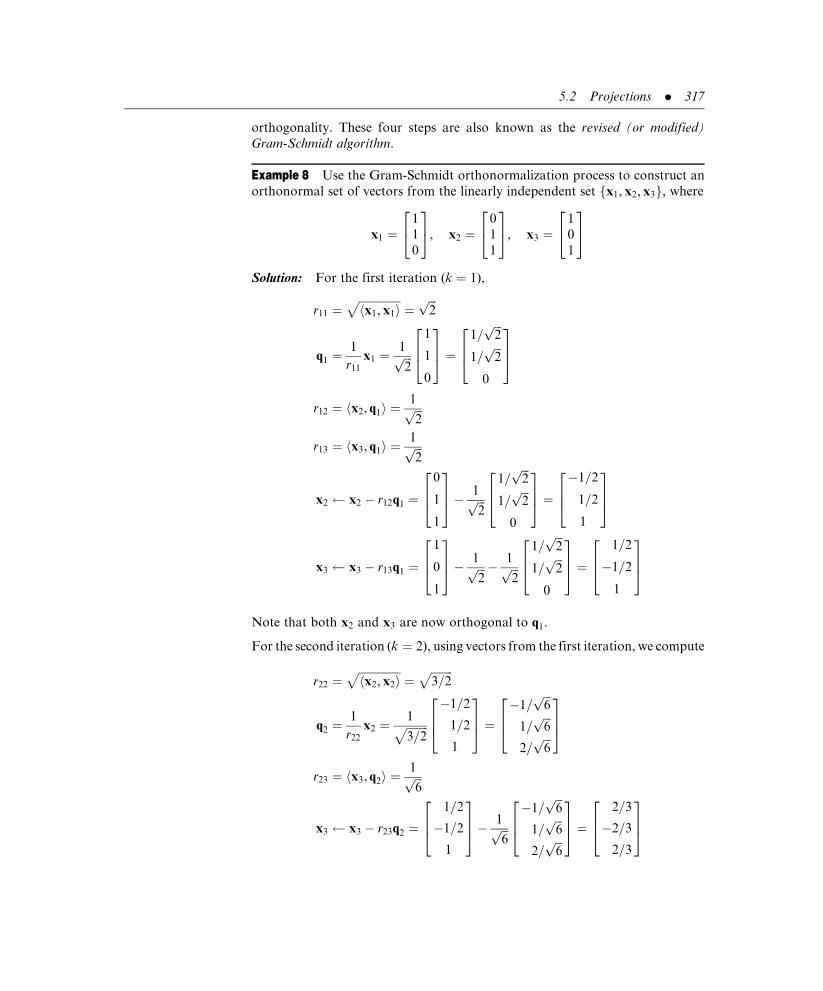
orthogonality. These four steps are also known as the revised (or modified)
Gram-Schmidt algorithm.
Example 8 Use the Gram-Schmidt orthonormalization process to construct an
orthonormal set of vectors from the linearly independent set fx1, x2, x3g, where
x1 ¼1
1
0
2435, x2 ¼
0
1
1
2435, x3 ¼
1
0
1
2435
Solution: For the first iteration (k ¼ 1),
r11 ¼ffiffiffiffiffiffiffiffiffiffiffiffiffiffiffihx1, x1i
p¼
ffiffiffi2p
q1 ¼1
r11
x1 ¼1ffiffiffi2p
1
1
0
264375 ¼ 1=
ffiffiffi2p
1=ffiffiffi2p
0
264
375
r12 ¼ hx2, q1i ¼1ffiffiffi2p
r13 ¼ hx3, q1i ¼1ffiffiffi2p
x2 x2 � r12q1 ¼0
1
1
264375� 1ffiffiffi
2p
1=ffiffiffi2p
1=ffiffiffi2p
0
264
375 ¼
�1=2
1=2
1
264
375
x3 x3 � r13q1 ¼1
0
1
264375� 1ffiffiffi
2p � 1ffiffiffi
2p
1=ffiffiffi2p
1=ffiffiffi2p
0
264
375 ¼
1=2
�1=2
1
264
375
Note that both x2 and x3 are now orthogonal to q1.
For the second iteration (k ¼ 2), using vectors from the first iteration, we compute
r22 ¼ffiffiffiffiffiffiffiffiffiffiffiffiffiffiffihx2, x2i
p¼
ffiffiffiffiffiffiffiffi3=2
p
q2 ¼1
r22
x2 ¼1ffiffiffiffiffiffiffiffi3=2
p �1=2
1=2
1
264
375 ¼ �1=
ffiffiffi6p
1=ffiffiffi6p
2=ffiffiffi6p
264
375
r23 ¼ hx3, q2i ¼1ffiffiffi6p
x3 x3 � r23q2 ¼1=2
�1=2
1
264
375� 1ffiffiffi
6p
�1=ffiffiffi6p
1=ffiffiffi6p
2=ffiffiffi6p
264
375 ¼
2=3
�2=3
2=3
264
375
5.2 Projections . 317

For the third iteration (k ¼ 3), using vectors from the second iteration, we compute
r33 ¼ffiffiffiffiffiffiffiffiffiffiffiffiffiffiffihx3, x3i
p¼ 2ffiffiffi
3p
q3 ¼1
r33
x3 ¼1
2=ffiffiffi3p
2=3�2=3
2=3
24
35 ¼ 1=
ffiffiffi3p
�1=ffiffiffi3p
1=ffiffiffi3p
24
35
The orthonormal set is fq1, q2, q3g: &
Example 9 Use the Gram-Schmidt orthonormalization process to construct an
orthonormal set of vectors from the linearly independent set fx1, x2, x3, x4g, where
x1 ¼
1
1
0
1
266664
377775, x2 ¼
1
2
1
0
266664
377775, x3 ¼
0
1
2
1
266664
377775, x4 ¼
1
0
1
1
266664
377775
Solution: Carrying eight significant figures through all computations but
rounding to four decimals for presentation purposes, we get
For the first iteration ( k ¼ 1 )
r11 ¼ffiffiffiffiffiffiffiffiffiffiffiffiffiffiffihx1, x1i
p¼
ffiffiffi3p¼ 1:7321,
q1 ¼1
r11
x1 ¼1ffiffiffi3p
1
1
0
1
266664
377775 ¼
0:5774
0:5774
0:0000
0:5774
266664
377775,
r12 ¼ hx2, q1i ¼ 1:7321,
r13 ¼ hx3, q1i ¼ 1:1547,
r14 ¼ hx4, q1i ¼ 1:1547,
x2 x2 � r12q1 ¼
1
2
1
0
266664
377775� 1:7321
0:5774
0:5774
0:0000
0:5774
266664
377775 ¼
0:0000
1:0000
1:0000
�1:0000
266664
377775,
x3 x3 � r13q1 ¼
0
1
2
1
2666437775� 1:1547
0:5774
0:5774
0:0000
0:5774
26664
37775 ¼
�0:6667
0:3333
2:0000
0:3333
26664
37775,
318 . Euclidean Inner Product

x4 x4 � r14q1 ¼
1
0
1
1
26643775� 1:1547
0:5774
0:5774
0:0000
0:5774
2664
3775 ¼
0:3333
�0:6667
1:0000
0:3333
2664
3775:
For the second iteration (k ¼ 2), using vectors from the first iteration, we
compute
r22 ¼ffiffiffiffiffiffiffiffiffiffiffiffiffiffiffihx2, x2i
p¼ 1:7321,
q2 ¼1
r22
x2 ¼1
1:7321
0:0000
1:0000
1:0000
�1:0000
266664
377775 ¼
0:0000
0:5774
0:5774
�0:5774
266664
377775,
r23 ¼ hx3, q2i ¼ 1:1547,
r24 ¼ hx4, q2i ¼ 0:0000,
x3 x3 � r23q2 ¼
�0:6667
0:3333
2:0000
0:3333
2666664
3777775� 1:1547
0:0000
0:5774
0:5774
�0:5774
2666664
3777775 ¼
�0:6667
�0:3333
1:3333
1:0000
2666664
3777775,
x4 x4 � r24q2 ¼
0:3333
�0:6667
1:0000
0:3333
2666664
3777775� 0:0000
0:0000
0:5774
0:5774
�0:5774
2666664
3777775 ¼
0:3333
�0:6667
1:0000
0:3333
2666664
3777775:
For the third iteration (k ¼ 3), using vectors from the second iteration,
we compute
r33 ¼ffiffiffiffiffiffiffiffiffiffiffiffiffiffiffihx3, x3i
p¼ 1:8257,
q3 ¼1
r33
x3 ¼1
1:8257
�0:6667
�0:3333
1:3333
1:0000
266664
377775 ¼
�0:3651
�0:1826
0:7303
0:5477
266664
377775,
r34 ¼ hx4, q3i ¼ 0:9129,
5.2 Projections . 319

x4 x4 � r34q3 ¼
0:3333
�0:6667
1:0000
0:3333
26664
37775� 0:9129
�0:3651
�0:1826
0:7303
0:5477
26664
37775 ¼
0:6667
�0:5000
0:3333
�0:1667
26664
37775:
For the fourth iteration (k ¼ 4), using vectors from the third iteration, we
compute
r44 ¼ffiffiffiffiffiffiffiffiffiffiffiffiffiffiffihx4, x4i
p¼ 0:9129,
q4 ¼1
r44
x4 ¼1
0:9129
0:6667
�0:5000
0:3333
�0:1667
266664
377775 ¼
0:7303
�0:5477
0:3651
�0:1826
266664
377775:
The orthonormal set is fq1, q2, q3, q4g. &
If B ¼ fx1, x2, . . . , xpg is a linearly independent set of vectors in an inner product
space U, and not necessarily a basis, then the Gram-Schmidt orthonormalization
process can be applied directly on B to transform it into an orthonormal set of
vectors with the same span as B. This follows immediately from Theorem 3
because B is a basis for the subspace V ¼ spanfx1, x2, . . . , xpg.
Problems 5.2
In Problems 1 through 10, determine (a) the projection of x1 onto x2, and (b) the
orthogonal component.
(1) x1 ¼1
2
� , x2 ¼
2
1
� . (2) x1 ¼
1
1
� , x2 ¼
3
5
� .
(3) x1 ¼3
�2
� , x2 ¼
3
3
� . (4) x1 ¼
4
�1
� , x2 ¼
2
8
� .
(5) x1 ¼�7
�2
� , x2 ¼
2
9
� . (6) x1 ¼
2
1
0
264375, x2 ¼
2
0
2
264375.
(7) x1 ¼1
1
0
264375, x2 ¼
2
2
1
264375. (8) x1 ¼
0
3
4
264375, x2 ¼
2
5
5
264375.
(9) x1 ¼
0
1
1
1
2666437775, x2 ¼
1
1
1
0
2666437775. (10) x1 ¼
1
2
3
4
2666437775, x2 ¼
1
�2
0
�1
26664
37775.
320 . Euclidean Inner Product

In Problems 11 through 23, show that the set B is an orthonormal basis (under the
Euclidean inner product or the inner product induced by the Euclidean inner product)
for the given vector space and then write x as a linear combination of those basis vectors.
(11) B ¼3=5
4=5
" #,
4=5
�3=5
" #( )in R2; x ¼ 3
5
� .
(12) B ¼ 1=ffiffiffi2p
1=ffiffiffi2p
" #,
1=ffiffiffi2p
�1=ffiffiffi2p
" #( )in R2; x ¼ 3
5
� .
(13) B ¼ 1=ffiffiffi5p
2=ffiffiffi5p
" #,�2=
ffiffiffi5p
1=ffiffiffi5p
" #( )in R2; x ¼ 2
�3
� .
(14) B ¼3=5
4=5
0
264
375,
4=5
�3=5
0
264
375,
0
0
1
264375
8><>:
9>=>; in R3; x ¼
1
2
3
2435.
(15) B ¼3=5
4=5
0
264
375,
4=5
�3=5
0
264
375,
0
0
1
264375
8><>:
9>=>; in R3; x ¼
10
0
�20
24
35.
(16) B ¼1=
ffiffiffi2p
1=ffiffiffi2p
0
264
375,
�1=ffiffiffi6p
1=ffiffiffi6p
2=ffiffiffi6p
264
375,
1=ffiffiffi3p
�1=ffiffiffi3p
1=ffiffiffi3p
264
375
8><>:
9>=>; in R3; x ¼
10
0
�20
24
35.
(17) B ¼�1=
ffiffiffi2p
1=ffiffiffi2p
0
264
375,
1=ffiffiffi6p
1=ffiffiffi6p
�2=ffiffiffi6p
264
375,
�1=ffiffiffi3p
�1=ffiffiffi3p
�1=ffiffiffi3p
264
375
8><>:
9>=>; in R3; x ¼
10
0
�20
24
35.
(18) B ¼ f0:6t� 0:8, 0:8tþ 0:6g in P1; x ¼ 2tþ 1.
(19) B ¼ f0:6t2 � 0:8, 0:8t2 þ 0:6, tg in P2; x ¼ t2 þ 2tþ 3.
(20) B ¼ f0:6t2 � 0:8, 0:8t2 þ 0:6, tg in P2; x ¼ t2 � 1.
(21) B ¼ 1=ffiffiffi3p
1=ffiffiffi3p
�1=ffiffiffi3p
0
" #(,
0 �1=ffiffiffi3p
�1=ffiffiffi3p
1=ffiffiffi3p
" #,
1=ffiffiffi3p
0
1=ffiffiffi3p
1=ffiffiffi3p
" #,
�1=ffiffiffi3p
1=ffiffiffi3p
0 1=ffiffiffi3p
" #)in M2�2; x ¼ 1 1
�1 2
� .
(22) B ¼3=5 4=5
0 0
� ,
4=5 �3=5
0 0
� ,
0 0
3=5 �4=5
� ,
0 0
�4=5 �3=5
� �;
in M2�2; x ¼1 2
3 4
� .
(23) B ¼1=2 1=2
1=ffiffiffi2p
0
� ,�1=2 �1=2
1=ffiffiffi2p
0
� ,�1=2 1=2
0 1=ffiffiffi2p
� ,
1=2 �1=2
0 1=ffiffiffi2p
� �
in M2�2; x ¼4 5
�6 7
� .
5.2 Projections . 321

In Problems 24 through 32, use the Gram-Schmidt orthonormalization process to
construct an orthonormal set from the given set of linearly independent vectors.
(24) The vectors in Problem 1.
(25) The vectors in Problem 2.
(26) The vectors in Problem 3.
(27) x1 ¼1
2
1
264375, x2 ¼
1
0
1
264375, x3 ¼
1
0
2
264375.
(28) x1 ¼2
1
0
264375, x2 ¼
0
1
1
264375, x3 ¼
2
0
2
264375.
(29) x1 ¼1
1
0
264375, x2 ¼
2
0
1
264375, x3 ¼
2
2
1
264375.
(30) x1 ¼0
3
4
264375, x2 ¼
3
5
0
264375, x3 ¼
2
5
5
264375.
(31) x1 ¼
0
1
1
1
2666437775, x2 ¼
1
0
1
1
2666437775, x3 ¼
1
1
0
1
2666437775, x4 ¼
1
1
1
0
2666437775.
(32) x1 ¼
1
1
0
0
2666437775, x2 ¼
0
1
�1
0
26664
37775, x3 ¼
1
0
�1
0
26664
37775, x4 ¼
1
0
0
�1
26664
37775.
(33) The vectors x1 ¼1
1
0
264375, x2 ¼
0
1
1
264375, x3 ¼
1
0
�1
264
375
are linearly dependent. Apply the Gram-Schmidt orthonormalization process to
them and use the results to deduce what occurs when the process is applied to
a linearly dependent set of vectors.
(34) Prove directly that x� ha, xiha, ai a is orthogonal to a.
(35) Prove that if x and y are orthonormal, then ksxþ tyk2 ¼ s2 þ t2 for any two scalars
s and t.
(36) Let Q be any n� n real matrix having columns that, when considered as n-dimen-
sional vectors, form an orthonormal set. What can one say about the product QTQ?
322 . Euclidean Inner Product

(37) Prove that if y, xh i ¼ 0 for every n-dimensional vector y, then x ¼ 0.
(38) Let A be an n� n real matrix and p be a real n-dimensional column matrix. Show
that if p is orthogonal to the columns of A, then Ay, ph i ¼ 0 for every n-dimensional
real column matrix y.
(39) Prove that if B is an orthonormal set of vectors that span a vector space U, then B is
a basis for U.
5.3 THE QR ALGORITHM
The QR algorithm is a robust numerical method for computing eigenvalues of
real matrices. In contrast to the power methods described in Section 4.6, which
converge to a single dominant real eigenvalue, the QR algorithm generally locates
all eigenvalues of a matrix, both real and complex, regardless of multiplicity.
To use the algorithm, we must factor a given matrix A into the matrix product
A ¼ QR (5:11)
where R is an upper (or right) triangular matrix and the columns of Q, con-
sidered as individual column matrices, form an orthonormal set. Equation (5.11)
is a QR decomposition of A. Such a decomposition is always possible when the
columns of A are linearly independent.
Example 1 Two QR decompositions are
1 3
1 5
" #¼
1=ffiffiffi2p
�1=ffiffiffi2p
1=ffiffiffi2p
1=ffiffiffi2p
" # ffiffiffi2p
4ffiffiffi2p
0ffiffiffi2p
" #and
1 2
2 2
2 1
264
375 ¼
1=3 10=ffiffiffiffiffiffiffiffi153p
2=3 2=ffiffiffiffiffiffiffiffi153p
2=3 �7=ffiffiffiffiffiffiffiffi153p
2664
3775 3 8=3
0ffiffiffiffiffiffiffiffi153p
=9
" #&
It is apparent from Example 1 that QR decompositions exist for square and
rectangular matrices. The orders of A and Q are the same and R is a square
matrix having the same number of columns as A. For the remainder of this
section, we restrict A to be square because we are interested in locating eigen-
values, and eigenvalues are defined only for square matrices. Then both Q and
R are square and have the same order as A.
A QR decomposition of a matrix A comes directly from the Gram-Schmidt ortho-
normalization process (see Theorem 3 of Section 5.2) applied to the linearly inde-
pendent columns ofA. The elements ofR ¼ [rij] are the scalars from Steps 1 and 3 of
the orthonormalization process, and the columns of Q are the orthonormal column
matrices constructed in Step 2 of that process. To see why, we let x(i)j denote xj after
the ith iteration of the Gram-Schmidt process ( j > i). Thus, x(1)j is the new value of
In a QR
decomposition of a
matrix A, the
elements of R ¼ [rij ]
are the scalars from
Steps 1 and 3 of the
Gram-Schmidt
orthonormalization
process applied to
the linearly
independent
columns of A, while
the columns of Q
are the orthonormal
column matrices
constructed in Step
2 of the Gram-
Schmidt process.
5.3 The QR Algorithm . 323
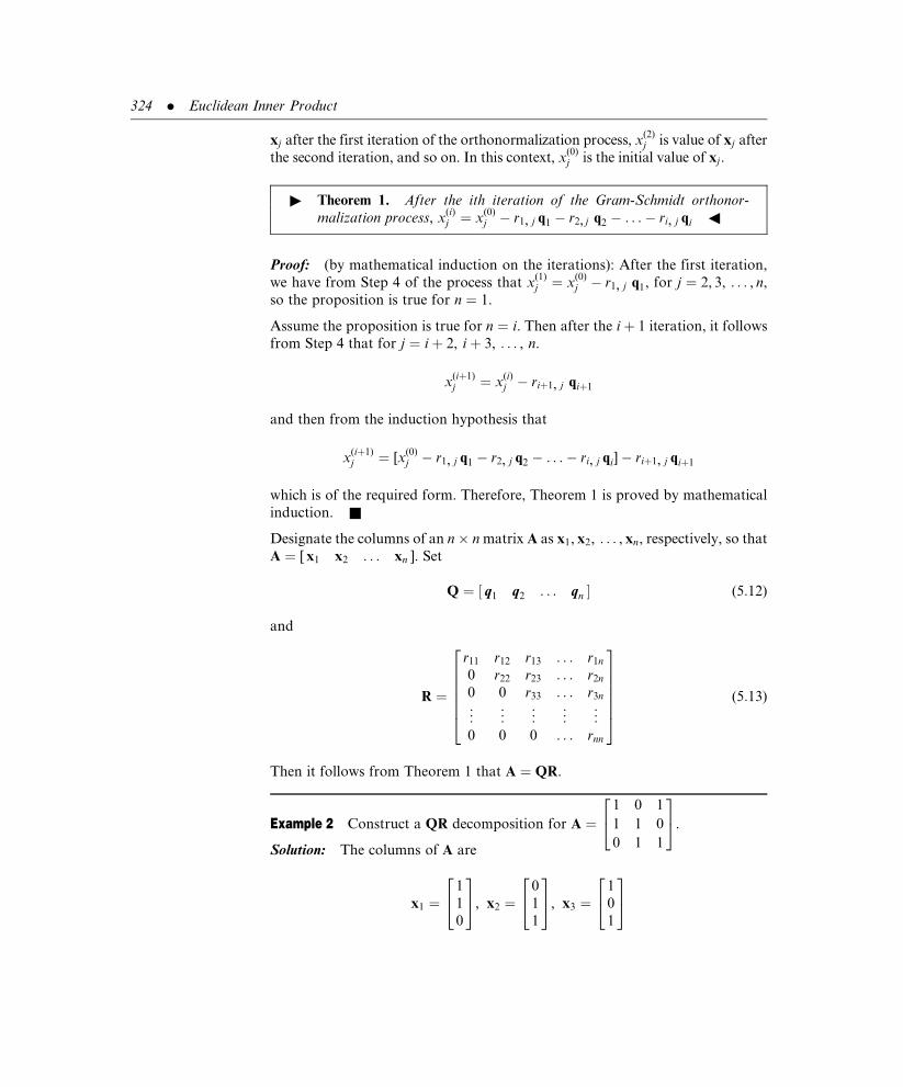
xj after the first iteration of the orthonormalization process, x(2)j is value of xj after
the second iteration, and so on. In this context, x(0)j is the initial value of xj.
" Theorem 1. After the ith iteration of the Gram-Schmidt orthonor-
malization process, x(i)j ¼ x
(0)j � r1, j q1 � r2, j q2 � . . .� ri, j qi 3
Proof: (by mathematical induction on the iterations): After the first iteration,
we have from Step 4 of the process that x(1)j ¼ x
(0)j � r1, j q1, for j ¼ 2, 3, . . . , n,
so the proposition is true for n ¼ 1.
Assume the proposition is true for n ¼ i. Then after the i þ 1 iteration, it follows
from Step 4 that for j ¼ i þ 2, i þ 3, . . . , n.
x(iþ1)j ¼ x
(i)j � riþ1, j qiþ1
and then from the induction hypothesis that
x(iþ1)j ¼ [x
(0)j � r1, j q1 � r2, j q2 � . . .� ri, j qi]� riþ1, j qiþ1
which is of the required form. Therefore, Theorem 1 is proved by mathematical
induction. &
Designate the columns of an n� n matrix A as x1, x2, . . . , xn, respectively, so that
A ¼ [ x1 x2 . . . xn ]. Set
Q ¼ q1 q2 . . . qn½ � (5:12)
and
R ¼
r11 r12 r13 . . . r1n
0 r22 r23 . . . r2n
0 0 r33 . . . r3n
..
. ... ..
. ... ..
.
0 0 0 . . . rnn
2666664
3777775 (5:13)
Then it follows from Theorem 1 that A ¼ QR.
Example 2 Construct a QR decomposition for A ¼1 0 1
1 1 0
0 1 1
24
35.
Solution: The columns of A are
x1 ¼1
1
0
2435, x2 ¼
0
1
1
2435, x3 ¼
1
0
1
2435
324 . Euclidean Inner Product

Using the results of Example 8 of Section 5.2, we have immediately that
Q ¼1=
ffiffiffi2p
�1=ffiffiffi6p
1=ffiffiffi3p
1=ffiffiffi2p
1=ffiffiffi6p
�1=ffiffiffi3p
0 2=ffiffiffi6p
1=ffiffiffi3p
24
35, R ¼
ffiffiffi2p
1=ffiffiffi2p
1=ffiffiffi2p
0ffiffiffiffiffiffiffiffi3=2
p1=
ffiffiffi6p
0 0 2=ffiffiffi3p
24
35
from which A ¼ QR. &
Example 3 Construct a QR decomposition for A ¼
1 1 0 1
1 2 1 0
0 1 2 1
1 0 1 1
2664
3775.
Solution: The columns of A are
x1 ¼
1
1
0
1
26643775, x2 ¼
1
2
1
0
26643775, x3 ¼
0
1
2
1
26643775, x4 ¼
1
0
1
1
26643775
Using the results of Example 9 of Section 5.2, we have immediately that
Q ¼
0:5774 0:0000 �0:3651 0:7303
0:5774 0:5774 �0:1826 �0:5477
0:0000 0:5774 0:7303 0:3651
0:5774 �0:5774 0:5477 �0:1826
26664
37775,
R ¼
1:7321 1:7321 1:1547 1:1547
0 1:7321 1:1547 0:0000
0 0 1:8257 0:9129
0 0 0 0:9129
26664
37775
from which A ¼ QR to within round-off error. &
The QR algorithm uses QR decompositions to identify the eigenvalues of
a square matrix. The algorithm involves many arithmetic calculations, making
it unattractive for hand computations but ideal for implementation on a com-
puter. Although a proof of the QR algorithm is beyond the scope of this book,
the algorithm itself is deceptively simple.
We begin with a square real matrix A0 having linearly independent columns.
To determine its eigenvalues, we create a sequence of new matrices
A1, A2, . . . , Ak�1, Ak, . . ., having the property that each new matrix has the
same eigenvalues as A0, and that these eigenvalues become increasingly obvious
as the sequence progresses. To calculate Ak (k ¼ 1, 2, . . . ) once Ak�1 is known,
we construct a QR decomposition of Ak�1:
5.3 The QR Algorithm . 325

Ak�1 ¼ Qk�1Rk�1
and then reverse the order of the product to define
Ak ¼ Rk�1Qk�1 (5:14)
Each matrix in the sequence fAkg has identical eigenvalues (see Problem 29), and
the sequence generally converges to one of the following two partitioned forms:
ð5:15Þ
or
ð5:16Þ
If matrix (5.15) occurs, then the element a is an eigenvalue, and the remaining
eigenvalues are found by applying the QR algorithm anew to the submatrix S. If,
on the other hand, matrix (5.16) occurs, then two eigenvalues are determined by
solving for the roots of the characteristic equation of the 2� 2 matrix in the
lower right partition, namely,
l2 � (bþ e)lþ (be� cd ) ¼ 0
The remaining eigenvalues are found by applying the QR algorithm anew to the
submatrix U.
Convergence of the algorithm is accelerated by performing a shift at each
iteration. If the orders of all matrices are n� n, we denote the element in the
(n, n) position of the matrix Ak�1 as wk�1, and construct a QR decomposition for
the shifted matrix Ak�1 � wk�1I. That is,
Ak�1 � wk�1I ¼ Qk�1Rk�1 (5:17)
We define
Ak ¼ Rk�1Qk�1 þ wk�1I (5:18)
Example 4 Find the eigenvalues of
A0 ¼0 1 0
0 0 1
18 �1 �7
24
35
Solution: Using the QR algorithm with shifting, carrying all calculations to eight
significant figures but rounding to four decimals for presentation, we compute
326 . Euclidean Inner Product

A0 � (� 7)I
¼7 1 0
0 7 1
18 �1 0
264
375
¼0:3624 0:1695 �0:9165
0:0000 0:9833 0:1818
0:9320 �0:0659 0:3564
264
375 19:3132 �0:5696 0:0000
0:0000 7:1187 0:9833
0:0000 0:0000 0:1818
264
375
¼ Q0R0
A1 ¼ R0Q0 þ (� 7)I
¼19:3132 �0:5696 0:0000
0:0000 7:1187 0:9833
0:0000 0:0000 0:1818
264
375 0:3624 0:1695 �0:9165
0:0000 0:9833 0:1818
0:9320 �0:0659 0:3564
264
375
þ�7 0 0
0 �7 0
0 0 �7
264
375
¼0:0000 2:7130 �17:8035
0:9165 �0:0648 1:6449
0:1695 �0:0120 �6:9352
264
375
A1 � (� 6:9352)I
¼6:9352 2:7130 �17:8035
0:9165 6:8704 1:6449
0:1695 �0:0120 0:0000
264
375
¼0:9911 �0:1306 �0:0260
0:1310 0:9913 0:0120
0:0242 �0:0153 0:9996
264
375 6:9975 3:5884 �17:4294
0:0000 6:4565 3:9562
0:0000 0:0000 0:4829
264
375
¼ Q1R1
A2 ¼ R1Q1 þ (� 6:9352)I ¼0:0478 2:9101 �17:5612
0:9414 �0:5954 4:0322
0:0117 �0:0074 �6:4525
24
35
5.3 The QR Algorithm . 327

Continuing in this manner, we generate sequentially
A3 ¼0:5511 2:7835 �16:8072
0:7826 �1:1455 6:5200
0:0001 �0:0001 �6:4056
264
375
A4 ¼0:9259 2:5510 �15:9729
0:5497 �1:5207 8:3583
0:0000 �0:0000 �6:4051
264
375
A4 has form (5.15) with
S ¼ 0:9259 2:5510
0:5497 �1:5207
� and a ¼ �6:4051
One eigenvalue is �6:4051, which is identical to the value obtained in
Example 2 of Section 4.6. In addition, the characteristic equation of R is
l2 þ 0:5948l� 2:8103 ¼ 0, which admits both �2 and 1.4052 as roots. These
are the other two eigenvalues of A0. &
Example 5 Find the eigenvalues of
A0 ¼
0 0 0 �25
1 0 0 30
0 1 0 �18
0 0 1 6
2664
3775
Solution: Using the QR algorithm with shifting, carrying all calculations to eight
significant figures but rounding to four decimals for presentation, we compute
A0 � (6)I ¼
�6 0 0 �25
1 �6 0 30
0 1 �6 �18
0 0 1 0
26664
37775
¼
�0:9864 �0:1621 �0:0270 �0:0046
0:1644 �0:9726 �0:1620 �0:0274
0:0000 0:1666 �0:9722 �0:1643
0:0000 0:0000 0:1667 �0:9860
26664
37775
�
6:0828 �0:9864 0:0000 29:5918
0:0000 6:0023 �0:9996 �28:1246
0:0000 0:0000 6:0001 13:3142
0:0000 0:0000 0:0000 2:2505
26664
37775
¼ Q0R0
328 . Euclidean Inner Product

A1 ¼ R0Q0 þ (6)I ¼
�0:1622 �0:0266 4:9275 �29:1787
0:9868 �0:0044 �4:6881 27:7311
0:0000 0:9996 2:3858 �14:1140
0:0000 0:0000 0:3751 3:7810
266664
377775
A1 � (3:7810)I ¼
�3:9432 �0:0266 4:9275 �29:1787
0:9868 �3:7854 �4:6881 27:7311
0:0000 0:9996 �1:3954 �14:1140
0:0000 0:0000 0:3751 0:0000
266664
377775
¼
�0:9701 �0:2343 �0:0628 �0:0106
0:2428 �0:9361 �0:2509 �0:0423
0:0000 0:2622 �0:9516 �0:1604
0:0000 0:0000 0:1662 �0:9861
266664
377775
�
4:0647 �0:8931 �5:9182 35:0379
0:0000 3:8120 2:8684 �22:8257
0:0000 0:0000 2:2569 8:3060
0:0000 0:0000 0:0000 1:3998
266664
377775
¼ Q1R1
A2 ¼ R1Q1 þ (3:7810)I
¼
�0:3790 �1:6681 11:4235 �33:6068
0:9254 0:9646 �7:4792 21:8871
0:0000 0:5918 3:0137 �8:5524
0:0000 0:0000 0:2326 2:4006
266664
377775
Continuing in this manner, we generate, after 25 iterations,
A25 ¼
4:8641 �4:4404 18:1956 �28:7675
4:2635 �2:8641 13:3357 �21:3371
0:0000 0:0000 2:7641 �4:1438
0:0000 0:0000 0:3822 1:2359
26664
37775
which has form (5.16) with
U ¼ 4:8641 �4:4404
4:2635 �2:8641
� and
b c
d e
� ¼ 2:7641 �4:1438
0:3822 1:2359
�
5.3 The QR Algorithm . 329

The characteristic equation of U is l2 � 2lþ 5 ¼ 0, which has as its roots
1� 2i; the characteristic equation of the other 2� 2 matrix is l2 � 4lþ 4:9999 ¼0, which has as its roots 2� i. These roots are the four eigenvalues of A0. &
Problems 5.3
In Problems 1 through 11, construct QR decompositions for the given matrices.
(1)1 2
2 1
� : (2)
1 3
1 5
� :
(3)3 3
�2 3
� : (4)
1 2
2 2
2 1
24
35:
(5)
1 1
1 0
3 5
24
35. (6)
3 1
�2 1
1 1
�1 1
2664
3775:
(7)
2 0 2
1 1 0
0 1 2
24
35: (8)
1 2 2
1 0 2
0 1 1
24
35:
(9)
0 3 2
3 5 5
4 0 5
24
35: (10)
0 1 1
1 0 1
1 1 0
1 1 1
2664
3775:
(11)
1 0 1
1 1 0
0 �1 �1
0 0 0
2664
3775:
(12) Discuss what is likely to happen in a QR decomposition of a matrix whose columns
are not linearly independent if all calculations are rounded to a finite number of
significant figures.
(13) Use one iteration of the QR algorithm to calculate A1 for
A0 ¼0 1 0
0 0 1
18 �1 7
24
35:
Note that this matrix differs from the one in Example 4 by a single sign.
(14) Use one iteration of the QR algorithm to calculate A1 for
A0 ¼2 �17 7
�17 �4 1
7 1 �14
24
35:
330 . Euclidean Inner Product
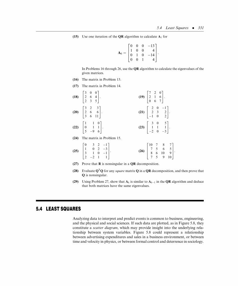
(15) Use one iteration of the QR algorithm to calculate A1 for
A0 ¼
0 0 0 �13
1 0 0 4
0 1 0 �14
0 0 1 4
2664
3775:
In Problems 16 through 26, use the QR algorithm to calculate the eigenvalues of the
given matrices.
(16) The matrix in Problem 13.
(17) The matrix in Problem 14.
(18)
3 0 0
2 6 4
2 3 5
24
35. (19)
7 2 0
2 1 6
0 6 7
24
35.
(20)
3 2 3
2 6 6
3 6 11
24
35. (21)
2 0 �1
2 3 2
�1 0 2
24
35.
(22)
1 1 0
0 1 1
5 �9 6
24
35. (23)
3 0 5
1 1 1
�2 0 �3
24
35.
(24) The matrix in Problem 15.
(25)
0 3 2 �1
1 0 2 �3
3 1 0 �1
2 �2 1 1
2664
3775. (26)
10 7 8 7
7 5 6 5
8 6 10 9
7 5 9 10
2664
3775.
(27) Prove that R is nonsingular in a QR decomposition.
(28) Evaluate QTQ for any square matrix Q in a QR decomposition, and then prove that
Q is nonsingular.
(29) Using Problem 27, show that Ak is similar to Ak�1 in the QR algorithm and deduce
that both matrices have the same eigenvalues.
5.4 LEAST SQUARES
Analyzing data to interpret and predict events is common to business, engineering,
and the physical and social sciences. If such data are plotted, as in Figure 5.8, they
constitute a scatter diagram, which may provide insight into the underlying rela-
tionship between system variables. Figure 5.8 could represent a relationship
between advertising expenditures and sales in a business environment, or between
time and velocity in physics, or between formal control and deterrence in sociology.
5.4 Least Squares . 331

The data in Figure 5.8 appears to follow a straight line relationship, but with
minor random distortions. Such distortions, called noise, are expected when data
are obtained experimentally. To understand why, assume you are asked to ride a
bicycle on a painted line down the middle of a straight path. A paint pot with a
mechanism that releases a drop of paint intermittently is attached to the bicycle
to check your accuracy. If you ride flawlessly, the paint spots will all fall on the
line you are to follow. A perfect ride, however, is not likely. Wind, road
imperfections, fatigue, and other random events will move the bicycle slightly
away from its intended path. Repeat this experiment three times, and the paint
spots from all three rides would look like the data points in Figure 5.8.
Generally, we have a set of data points obtained experimentally from a process
of interest, such as those in Figure 5.8, and we want the equation of the
underlying theoretical relationship. For example, we have the spots left by
a bicycle, and we want the equation of the path the rider followed. In this
section, we limit ourselves to relationships that appear linear.
A straight line in the variables x and y satisfying the equation
y ¼ mxþ c (5:19)
Small random
variations from
expected patterns
are called noise.
Figure 5.8 y
x
Figure 5.9
1 2 3 4
3
2
1
6
5
4
7
9
8
10
y
x0
��
�
�
� e (4)
e (3)
e (2)
e (0)
e (1)
Denotes a data point
y = 2
x + 1
.5
Denotes a point on the straight line for the samex-value as the data point
�
332 . Euclidean Inner Product

where m and c are constants, will have one y value on the line for each value of x.
This y value may not agree with the data at each value of x where data exists (see
Figure 5.9). The difference between the y value of the data point at x and the y
value defined by equation (5.19) for this same value of x is known as the residual
at x, which we denote as e(x).
Example 1 Calculate the residuals between the five data points in Figure 5.9
and their corresponding points on the line defined by y ¼ 2xþ 1:5.
Solution: Data points are provided at x ¼ 0, x ¼ 1, x ¼ 2, x ¼ 3, and x ¼ 4.
Evaluating the equation y ¼ 2xþ 1:5 at these values of x, we generate Table 5.1.
The residuals are
e(0) ¼ 1� 1:5 ¼ �0:5
e(1) ¼ 5� 3:5 ¼ 1:5
e(2) ¼ 3� 5:5 ¼ �2:5
e(3) ¼ 6� 7:5 ¼ �1:5
e(4) ¼ 9� 9:5 ¼ �0:5
Note that these residuals can be read directly from Figure 5.9. &
In general, we have N data points at (x1, y1), (x2, y2), (x3, y3), . . . , (xN , yN) with
residuals e(x1), e(x2), e(x3), . . . , e(xN ) between the data points and a straight line
approximation to the data. Residuals may be positive, negative, or 0, with a zero
residual occurring only when a data point is on the straight line approximation.
The least-squares error E is the sum of the squares of the individual residuals.
That is,
E ¼ [e(x1)]2 þ [e(x2)]
2 þ [e(x3)]2 þ . . .þ [e(xN)]2
The least-squares error is 0 if and only if all the residuals are 0.
TABLE 5.1
Given data
Evaluated from
y ¼ 2xþ 1:5
x y y
0 1 1.5
1 5 3.5
2 3 5.5
3 6 7.5
4 9 9.5
5.4 Least Squares . 333

Example 2 Calculate the least-squares error made in approximating the data in
Figure 5.9 by the straight line defined by y ¼ 2xþ 1:5.
Solution: Using the residuals determined in Example 1, we have
E ¼ [e(0)]2 þ [e(1)]2 þ [e(2)]2 þ [e(3)]2 þ [e(4)]2
¼ (� 0:5)2 þ (1:5)2 þ (� 2:5)2 þ (� 1:5)2 þ (� 0:5)2
¼ 0:25þ 2:25þ 6:25þ 2:25þ 0:25
¼ 11:25 &
Corresponding to every straight line approximation to a given set of data is a set
of residuals and a least-squares error. Different straight lines can produce
different least-squares errors, and we define the least-squares straight line to be
the line that minimizes the least-squares error. A nonvertical straight line satisfies
the equation
y ¼ mxþ c (5:19 repeated)
and has residuals
e(xi) ¼ yi � (mxi þ c)
at xi (i ¼ 1, 2, . . . ,N). We seek values of m and c that minimize
E ¼XNi¼1
( yi �mxi � c)2
This occurs when
@E
@m¼XNi¼1
2( yi �mxi � c)(� xi) ¼ 0
@E
@c¼XNi¼1
2( yi �mxi � c)(� 1) ¼ 0
or, upon simplifying, when
XNi¼1
x2i
!mþ
XNi¼1
xi
!c ¼
XNi¼1
xiyi
XNi¼1
xi
!mþNc ¼
XNi¼1
yi
(5:20)
System (5.20) makes up the normal equations for a least-squares fit in two
variables.
The least-squares
error is the sum of
the squares of the
individual residuals,
and the least-
squares straight line
is the line that
minimizes the least-
squares error.
334 . Euclidean Inner Product

Example 3 Find the least-squares straight line for the following xy data:
x 0 1 2 3 4
y 1 5 3 6 9
Solution: Table 5.2 contains the required summations. For this data, the nor-
mal equations become
30mþ 10c ¼ 65
10mþ 5c ¼ 24
which has as its solution m ¼ 1:7 and c ¼ 1:4. The least-squares straight line is
y ¼ 1:7xþ 1:4. &
The normal equations have a simple matrix representation. Ideally, we would
like to choose m and c for (5.19) so that,
yi ¼ mxi þ c
for all data pairs (xi, yi), i ¼ 1, 2, . . . , N. That is, we want the constants m and c
to solve the system
mx1 þ c ¼ y1
mx2 þ c ¼ y2
mx3 þ c ¼ y3
..
.
mxN þ c ¼ yN
or, equivalently, the matrix equation
x1 1
x2 1
x3 1
..
. ...
xN 1
2666664
3777775
m
c
� ¼
y1
y2
y3
..
.
yN
2666664
3777775
TABLE 5.2
xi yi (xi)2 xiyi
0 1 0 0
1 5 1 5
2 3 4 6
3 6 9 18
4 9 16 36
X5
i¼1
xi ¼ 10X5
i¼1
yi ¼ 24X5
i¼1
(xi)2 ¼ 30
X5
i¼1
xiyi ¼ 65
5.4 Least Squares . 335

This system has the standard form Ax ¼ b, where A is defined as a matrix having
two columns, the first being the data vector [ x1 x2 x3 � � � xN ]T, and the
second containing all ones, x ¼ [ m c ]T, and b is the data vector
[ y1 y2 y3 � � � yN ]T. In this context, Ax ¼ b has a solution for x if and
only if the data falls on a straight line. If not, then the matrix system is
inconsistent, and we seek the least-squares solution. That is, we seek the vector
x that minimizes the least-squares error having the matrix form
E ¼ kAx� bk2 (5:21)
The solution is the vector x satisfying the normal equations, which take the
matrix form
ATAx ¼ ATb (5:22)
System (5.22) is identical to system (5.20) when A and b are as just defined.
We now generalize to all linear systems of the form Ax ¼ b. We are primarily
interested in cases where the system is inconsistent (rendering the methods
developed in Chapter 1 useless), and this generally occurs when A has more
rows than columns. We place no restrictions on the number of columns in A, but
we will assume that the columns are linearly independent. We seek the vector x
that minimizes the least-squares error defined by Eq. (5.21).
" Theorem 1. If x has the property that Ax� b is orthogonal to the
columns of A, then x minimizes kAx� bk2. 3
Proof: For any vector x0 of appropriate dimension,
kAx0 � bk2 ¼ k(Ax0 � Ax)þ (Ax� b)k2
¼ h(Ax0 � Ax)þ (Ax� b), (Ax0 � Ax)þ (Ax� b)i
¼ h(Ax0 � Ax), (Ax0 � Ax)i þ h(Ax� b), (Ax� b)i
þ 2h(Ax0 � Ax), (Ax� b)i
¼ k(Ax0 � Ax)k2 þ k(Ax� b)k2
þ 2h(Ax0, (Ax� b)i � 2hAx, (Ax� b)i
It follows directly from Problem 38 of Section 5.2 that the last two inner
products are both 0 (take p ¼ Ax� b). Therefore,
kAx0 � bk2 ¼ k(Ax0 � Ax)k2 þ k(Ax� b)k2
k(Ax� b)k2
and x minimizes Eq. (5.21). &
336 . Euclidean Inner Product

As a consequence of Theorem 1, we seek a vector x having the property that
Ax� b is orthogonal to the columns of A. Denoting the columns of A as
A1, A2, . . . , An, respectively, we require
hAi, Ax� bi ¼ 0 (i ¼ 1, 2, . . . , n)
If y ¼ [ y1 y2 � � � yn ]T denotes an arbitrary vector of appropriate dimension,
then
Ay ¼ A1y1 þ A2y2 þ � � � þ Anyn ¼Xn
i¼1
Aiyi
hAy, (Ax� b)i ¼Xn
i¼1
Aiyi, (Ax� b)
* +
¼Xn
i¼1
hAiyi, (Ax� b)i
¼Xn
i¼1
yihAi, (Ax� b)i
¼ 0 (5:23)
It follows from
hx, yi ¼ xTy (5:2 repeated)
that
hAy, (Ax� b)i ¼ (Ay)T(Ax� b)
¼ (yTAT)(Ax� b)
¼ yT(ATAx� ATb)
¼ hy, (ATAx� ATb)i (5:24)
Equations (5.23) and (5.24) imply that hy, (ATAx� ATb)i ¼ 0 for any y. Using
the results of Problem 37 of Section 5.2, we conclude that (ATAx� ATb) ¼ 0 or
that ATAx ¼ ATb, which has the same form as equation (5.22)! Thus, we have
Theorem 2.
" Theorem 2. A vector x is the least-squares solution to Ax ¼ b if and
only if x is a solution to the normal equations ATAx ¼ ATb. 3
5.4 Least Squares . 337

The set of normal equations has a unique solution whenever the columns of A
are linearly independent, and these normal equations may be solved using any of
the methods presented in the previous chapters for solving systems of simultan-
eous linear equations.
Example 4 Find the least-squares solution to
xþ 2yþ z ¼ 1
3x� y ¼ 2
2xþ y� z ¼ 2
xþ 2yþ 2z ¼ 1
Solution: This system takes the matrix form Ax ¼ b, with
A ¼
1 2 1
3 �1 0
2 1 �1
1 2 2
26664
37775, x ¼
x
y
z
2435, and b ¼
1
2
2
1
2666437775
Then,
ATA ¼15 3 1
3 10 5
1 5 6
24
35 and ATb ¼
12
4
1
24
35
and the normal equations become
15 3 1
3 10 5
1 5 6
24
35 x
y
z
2435 ¼ 12
4
1
24
35
Using Gaussian elimination, we obtain as the unique solution to this set of
equations x ¼ 0:7597, y ¼ 0:2607, and z ¼ �0:1772, rounded to four decimals,
which is also the least-squares solution to the original system. &
Example 5 Find the least-squares solution to
0xþ 3y ¼ 80
2xþ 5y ¼ 100
5x� 2y ¼ 60
�xþ 8y ¼ 130
10x� y ¼ 150
338 . Euclidean Inner Product

Solution: This system takes the matrix form Ax ¼ b, with
A ¼
1 3
2 5
5 �2
�1 8
10 �1
266664
377775, x ¼ x
y
� , and b ¼
80
100
60
130
150
266664
377775
Then,
ATA ¼ 131 �15
�15 103
� and ATb ¼ 1950
1510
�
and the normal equations become
131 �15
�15 103
� x
y
� ¼ 1950
1510
�
The unique solution to this set of equations is x ¼ 16:8450 and y ¼ 17:1134,
rounded to four decimals, which is also the least-squares solution to the original
system. &
Problems 5.4
In Problems 1 through 8, find the least-squares solution to the given systems of equations.
(1) 2xþ 3y ¼ 8,
3x� y ¼ 5,
xþ y ¼ 6:
(2) 2xþ y ¼ 8,
y ¼ 4,
�xþ y ¼ 0,
3xþ y ¼ 13:
(3) xþ 3y ¼ 65,
2x� y ¼ 0,
3xþ y ¼ 50,
2xþ 2y ¼ 55:
(4) 2xþ y ¼ 6,
xþ y ¼ 8,
�2xþ y ¼ 11,
�xþ y ¼ 8,
3xþ y ¼ 4:
(5) 2xþ 3y� 4z ¼ 1,
x� 2yþ 3z ¼ 3,
xþ 4yþ 2z ¼ 6,
2xþ y� 3z ¼ 1:
(6) 2xþ 3yþ 2z ¼ 25,
2x� yþ 3z ¼ 30,
3xþ 4y� 2z ¼ 20,
3xþ 5yþ 4z ¼ 55:
(7) xþ y� z ¼ 90,
2xþ yþ z ¼ 200,
xþ 2yþ 2z ¼ 320,
3x� 2y� 4z ¼ 10,
3xþ 2y� 3z ¼ 220:
(8) xþ 2yþ 2z ¼ 1,
2xþ 3yþ 2z ¼ 2,
2xþ 4yþ 4z ¼ �2,
3xþ 5yþ 4z ¼ 1,
xþ 3yþ 2z ¼ �1:
5.4 Least Squares . 339
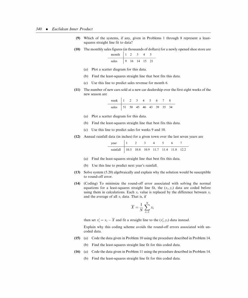
(9) Which of the systems, if any, given in Problems 1 through 8 represent a least-
squares straight line fit to data?
(10) The monthly sales figures (in thousands of dollars) for a newly opened shoe store are
month 1 2 3 4 5
sales 9 16 14 15 21
(a) Plot a scatter diagram for this data.
(b) Find the least-squares straight line that best fits this data.
(c) Use this line to predict sales revenue for month 6.
(11) The number of new cars sold at a new car dealership over the first eight weeks of the
new season are
week 1 2 3 4 5 6 7 8
sales 51 50 45 46 43 39 35 34
(a) Plot a scatter diagram for this data.
(b) Find the least-squares straight line that best fits this data.
(c) Use this line to predict sales for weeks 9 and 10.
(12) Annual rainfall data (in inches) for a given town over the last seven years are
year 1 2 3 4 5 6 7
rainfall 10.5 10.8 10.9 11.7 11.4 11.8 12.2
(a) Find the least-squares straight line that best fits this data.
(b) Use this line to predict next year’s rainfall.
(13) Solve system (5.20) algebraically and explain why the solution would be susceptible
to round-off error.
(14) (Coding) To minimize the round-off error associated with solving the normal
equations for a least-squares straight line fit, the (xi, yi) data are coded before
using them in calculations. Each xi value is replaced by the difference between xi
and the average of all xi data. That is, if
X ¼ 1
N
XNi¼1
xi
then set x0i ¼ xi � X and fit a straight line to the (x0i, yi) data instead.
Explain why this coding scheme avoids the round-off errors associated with un-
coded data.
(15) (a) Code the data given in Problem 10 using the procedure described in Problem 14.
(b) Find the least-squares straight line fit for this coded data.
(16) (a) Code the data given in Problem 11 using the procedure described in Problem 14.
(b) Find the least-squares straight line fit for this coded data.
340 . Euclidean Inner Product

(17) Census figures for the population (in millions of people) for a particular region of
the country are as follows:
year 1950 1960 1970 1980 1990
population 25.3 23.5 20.6 18.7 17.8
(a) Code this data using the procedure described in Problem 14, and then find the
least-squares straight line that best fits it.
(b) Use this line to predict the population in 2000.
(18) Show that if A ¼ QR is a QR decomposition of A, then the normal equations given
by Eq. (5.22) can be written as RTRx ¼ RTQTb, which reduces to Rx ¼ QTb. This is
a numerically stable set of equations to solve, not subject to the same round-off
errors associated with solving the normal equations directly.
(19) Use the procedure described in Problem 18 to solve Problem 1.
(20) Use the procedure described in Problem 18 to solve Problem 2.
(21) Use the procedure described in Problem 18 to solve Problem 5.
(22) Use the procedure described in Problem 18 to solve Problem 6.
(23) Determine the column matrix of residuals associated with the least-squares solution
of Problem 1, and then calculate the inner product of this vector with each of the
columns of the coefficient matrix associated with the given set of equations.
(24) Determine the column matrix of residuals associated with the least-squares solution
of Problem 5, and then calculate the inner product of this vector with each of the
columns of the coefficient matrix associated with the given set of equations.
5.5 ORTHOGONAL COMPLEMENTS
Two vectors in the same inner product space are orthogonal if their inner
product is zero. More generally, we say that the two subspaces U and W of an
inner product space V are orthogonal, written U?W, if u, wh i ¼ 0 for every u 2 U
and every w 2W.
Example 1 The subspaces
U ¼ fat2 þ btþ c 2 P2jb ¼ 0g and W ¼ fat2 þ btþ c 2 P2ja ¼ c ¼ 0g
are orthogonal with respect to the induced Euclidean inner product. If p(t) 2 U,
then p(t) ¼ at2 þ c, for some choice of the real numbers a and c. If q(t) 2W, then
q(t) ¼ bt for some choice of the real number b. Then
h p(t), q(t) i ¼ hat2 þ c, bti ¼ hat2 þ 0tþ c, 0t2 þ btþ 0i
¼ a(0)þ 0(b)þ c(0) ¼ 0 &
Two subspaces U
and W of the inner
product space V are
orthogonal if
u,wh i ¼ 0 for every
u 2 U and every
w 2W.
5.5 Orthogonal Complements . 341

Example 2 The subspaces U ¼ span 1 1 1½ �T, 1 �1 0½ �Tn o
and
W ¼ span 1 1 �2½ �Tn o
in R3 are orthogonal with respect to the Euclidean
inner product. Every vector in u 2 U must have the form
u ¼ a
1
1
1
2435þ b
1
�1
0
24
35 ¼ aþ b
a� b
a
24
35
for some choice of scalars a and b, while every vector in w 2W must have the
form
w ¼ c
1
1
�2
24
35 ¼ c
c
�2c
24
35
for some choice of scalar c. Here,
u, wh i ¼ (aþ b)(c)þ (a� b)(c)þ a(� 2c) ¼ 0 &
Orthogonal subspaces in R3 do not always agree with our understanding of
perpendicularity. The xy-plane is perpendicular to the yz-plane, as illustrated
in Figure 5.10, but the two planes are not orthogonal. The xy-plane is the
subspace defined by
U ¼ x y z½ �T2 R3jz ¼ 0n o
Therefore, u ¼ 1 1 0½ �T is a vector in U. The yz-plane is the subspace defined
by
W ¼ x y z½ �T2 R3jx ¼ 0n o
Figure 5.10
yz - plane
xy - plane
z
x
y
342 . Euclidean Inner Product

and w ¼ 0 1 1½ �T is in W. Here,
u, vh i ¼ 1(0)þ 1(1)þ 0(1) ¼ 1 6¼ 0
If U is a subspace of an inner product space V, we define the orthogonal
complement of U, denoted as U?, as the set of all vectors in V that are orthogonal
to every vector in U, that is,
U? ¼ v 2 Vj u, vh i ¼ 0 for every u 2 Uf g (5:25)
Example 3 In R3, the orthogonal complement of the z-axis is the xy-plane. The
z-axis is the subspace
Y ¼ x y z½ �T2 R3jx ¼ y ¼ 0n o
so any vector in this subspace has the form 0 0 a½ �T for some choice of the
scalar a. A general vector in R3 has the form x y z½ �T for any choice of the
scalars x, y, and z. If
xyz
" #,
000
" #* +¼ za
is to be zero for every choice of the scalar a, then z ¼ 0. Thus, the orthogonal
complement of the z-axis is the set
x y z½ �T2 R3jz ¼ 0n o
which defines the xy-plane. &
" Theorem 1. If U is a subspace of an inner product space V, then so too
is the orthogonal complement of U. 3
Proof: Let x and y be elements of U?, and let u 2 U. Then x, uh i ¼ 0, y, uh i ¼ 0,
and for any two scalars a and b
axþ by, uh i ¼ ax, uh i þ by, uh i ¼ a x, uh i þ b y, uh i ¼ a(0)þ b(0) ¼ 0:
Thus, axþ by 2 U? and U? is a subspace of V. &
" Theorem 2. If U is a subspace of an inner product space V, then the
only vector common to both U and U? is the zero vector. 3
If U is a subspace of
an inner product
space V, then U?,
the orthogonal
complement of U, is
the set of all vectors
in V that are
orthogonal to every
vector in U.
5.5 Orthogonal Complements . 343
Proof: Let x be a vector in both U and U?. Since x 2 U?, it must be orthogonal
to every vector in U, hence x must be orthogonal to itself, because x 2 U. Thus,
x, xh i ¼ 0, and it follows immediately from Theorem 1 of Section 5.1 that
x ¼ 0. &
Identifying the orthogonal complement of subspaces U of Rn is straightforward
when we know a spanning set S ¼ fu1, u2, . . . , ukg for U. We define a matrix A to
be
A ¼
uT1
uT2
..
.
uTk
2666664
3777775 (5:26)
where the column matrices in S become the rows of A. We then transform A to
row-reduced form using elementary row operations, obtaining
A!
vT1
vT2
..
.
vTk
2666664
3777775
The nonzero rows of this row-reduced matrix are a basis for U. Any vector
x 2 U? must be orthogonal to each basis vector in U, so
vj, x� �
¼ 0 ( j ¼ 1, 2, . . . , k): (5:27)
Equation (5.27) yields a set of k equations (some of which will be 0 ¼ 0 when the
rank of A is less than k) for the components of x. These equations define all
vectors in the orthogonal complement of U. But equation (5.27) also defines the
kernel of the matrix A in equation (5.26), so we have proven Theorem 3.
" Theorem 3. If S is a spanning set for a subspace U of Rn (considered as
column matrices) and if a matrix A is created so that each row of A is the
transpose of the vectors in S, then U? ¼ ker(A). 3
Example 4 Find the orthogonal complement of the subspace in R4 spanned by
S ¼
1
3
1
�1
2664
3775,
2
7
2
1
26643775,
1
4
1
2
26643775
8>><>>:
9>>=>>;
344 . Euclidean Inner Product

Solution: For these vectors, matrix (5.26) becomes
A ¼1 3 1 �1
2 7 2 1
1 4 1 2
24
35
which is transformed by elementary row operation to the row-reduced form
!1 3 1 �1
0 1 0 3
0 1 0 3
264
375
!1 3 1 �1
0 1 0 3
0 0 0 0
264
375
A basis for U is 1 3 1 �1½ �T, 0 1 0 3½ �Tn o
, hence U is a two-dimen-
sional subspace of R4. If we let x ¼ x1, x2, x3, x1½ �T, denote an arbitrary element
in the kernel of A, then
x1 þ 3x2 þ x3 � x4 ¼ 0
x2 þ 3x4 ¼ 0
0 ¼ 0
whence, x1 ¼ �x3 þ 10x4, x2 ¼ �3x4 with x3 and x4 arbitrary. Thus the kernel
of A is
�x3 þ 10x4
�3x4
x3
x4
2664
3775 ¼ x3
�1
0
1
0
2664
3775þ x4
10
�3
0
1
2664
3775x3 and x4 are arbitrary
8>><>>:
9>>=>>;
A basis for U? is �1 0 1 0½ �T, 10 �3 0 1½ �Tn o
, and UT is also a two-
dimensional subspace of R4. &
" Theorem 4. If U is a subspace of Rn, then dim(U)þ dim(U?) ¼ n. 3
Proof: The proposition is true when U ¼ f0g, because h0, yi ¼ 0 for every
y 2 Rn and U? ¼ Rn. In all other cases, let S ¼ u1, u2, . . . , ukf g be a basis for
U, and construct A as in equation (5.26). Then A is a linear transformation from
Rn to Rk. Because S is a basis, r(A) ¼ dim(U) ¼ k, where r(A) denotes the rank of
A. The nullity of A, v(A), is the dimension of the kernel of A, hence v(A) is the
dimension of U?. But r(A)þ v(A) ¼ n (Corollary 1 of Section 3.5), so Theorem 4
is immediate. &
5.5 Orthogonal Complements . 345

" Theorem 5. If U is a subspace of Rn, then (U?)? ¼ U. 3
Proof: If u 2 U, then u is orthogonal to every vector in U?, so u 2 (U?)? and
U is a subset of (U?)?. Denote the dimension of U as k. It follows from Theorem
4 that dim(U?) ¼ n� k. But it also follows from Theorem 4 that
dim(U?)þ dim((U?)?) ¼ n, whereupon dim((U?)?) ¼ n� (n� k) ¼ k ¼ dim(U).
Thus, U (U?)? with each subspace having the same dimension, hence
U ¼ (U?)?. &
We began Section 5.2 by writing a vector x 2 R2 as the sum of two vectors uþ v;which were orthogonal to one another. We now do even more.
" Theorem 6. If U is a subspace of Rn, then each vector x 2 Rn can be
written uniquely as x ¼ uþ u?, where u 2 U and u? 2 U?. 3
Proof: If U ¼ Rn, then U? ¼ f0g; and, conversely, if U ¼ f0g, then U? ¼ Rn,
because x ¼ xþ 0 ¼ 0þ x. In all other cases, let u1, u2, . . . , ukf g be a basis for
U(k < n), and let ukþ1, ukþ2, . . . , unf g be a basis for U?. We first claim that the
set S ¼ u1, u2, . . . , uk, ukþ1, ukþ2, . . . , unf g is linearly independent, which is
equivalent to showing that the only solution to
c1u1 þ c2u2 þ . . .þ ckuk þ ckþ1ukþ1 þ ckþ2ukþ2 þ . . .þ cnun ¼ 0 (5:28)
is c1 ¼ c2 ¼ . . . ¼ cn ¼ 0. If we rewrite equation (5.28) as
c1u1 þ c2u2 þ . . .þ ckuk ¼ �ckþ1ukþ1 � ckþ2ukþ2 � . . .� cnun
we see that the left side of this equation is a vector in U while the right side is
a vector in U?. Since the vectors are equal, they represent a vector in both U and
U? that, from Theorem 2, must be the zero vector. Thus,
c1u1 þ c2u2 þ . . .þ ckuk ¼ 0
and since u1, u2, . . . , ukf g is a linearly independent set (it is a basis for U), we
conclude that c1 ¼ c2 ¼ . . . ¼ ck ¼ 0. Similarly
ckþ1ukþ1 þ ckþ2ukþ2 þ . . .þ cnun ¼ 0
and since ukþ1, ukþ2, . . . , unf g is a linearly independent set (it is as basis for U?),
we conclude that ckþ1 ¼ ckþ2 ¼ . . . ¼ cn ¼ 0. Thus, S is linearly independent as
claimed.
Since the dimension of Rn is n and S is a linearly independent set of n-vectors in
Rn, it follows that S is a basis for Rn. We now have (see Theorem 5 of Section
2.4) that each vector in Rn can be written uniquely as a linear combination of the
346 . Euclidean Inner Product

vectors in S. That is, if x 2 Rn, then there exists a unique set of scalars
d1 ¼ d2 ¼ . . . ¼ dn such that
x ¼ d1u1 þ d2u2 þ . . .þ dkuk þ dkþ1ukþ1 þ dkþ2ukþ2 þ . . .þ dnun
Setting u ¼ d1u1 þ d2u2 þ . . .þ dkuk and u? ¼ dkþ1ukþ1 þ dkþ2ukþ2 þ . . .þ dnun,
we have u 2 U, u? 2 U?, and x ¼ uþ u?. &
Example 5 Decompose x ¼ �14 �10 12½ �T into the sum of two vectors, one
in the subspace U spanned by 1 1 5½ �T, 2 �1 1½ �Tn o
and the other in U?.
Solution: The vectors u1 ¼ 1 1 5½ �T and u2 ¼ 2 �1 1½ �T are linearly
independent, so they form a basis for U. We set
A ¼ 1 1 5
2 �1 1
�
and then determine that u3 ¼ �2 �2 1½ �T is a basis for ker(A) (see Example 1
of Section 3.5) and, therefore, a basis for U?. Thus, B ¼ u1, u2, u3f g is a basis for
R3.
We want the coordinates of the given vector x ¼ �14 �10 12½ �T with respect
to the B basis; that is, we want the values of the scalars d1, d2, and d3 so that
d1
1
1
5
2435þ d2
2
�1
5
24
35þ d3
�2
�3
1
24
35 ¼ �14
�10
12
24
35:
Solving the associated system of simultaneous linear equations by Gaussian
elimination, we find d1 ¼ 2, d2 ¼ �3; and d3 ¼ 5. Finally setting
u ¼ 2u1 þ (� 3)u2 ¼ 2
1
1
5
264375þ (� 3)
2
�1
5
264
375 ¼ �4
5
7
264
375
u? ¼ 5u3 ¼�10
�15
5
264
375
we have u 2 U, u??U?, and x ¼ uþ u?. &
Whenever we have a decomposition of a given vector x into the sum of two
vectors as described in Theorem 6, x ¼ uþ u?, then u is called the projection of
x on U. In the special case where U is a one-dimensional subspace spanned by
a single vector a, the projection of x on U is obtained most easily by equation
(5.6) in Section 5.2.
5.5 Orthogonal Complements . 347

Example 6 Using the results of Example 5, we have that u ¼ �4 5 7½ �T is the
projection of the vector x ¼ �14 �10 12½ �T on the subspace U spanned by
1 1 5½ �T, 2 �1 1½ �Tn o
. &
A vector space V is the direct sum of two subspaces U and W, written
V ¼ U�W, if each vector in V can be written uniquely as the sum uþ v, where
u 2 U and v 2 V. It follows from Theorem 6 that Rn ¼ U� U? for each subspace
U of Rn.
Problems 5.5
In Problems 1 through 10, (a) find the orthogonal complement for the subspace U of R3
spanned by the given set of vectors, and then (b) find the projection of x ¼ 1 1 0½ �Ton U.
(1) 0 1 1½ �Tn o
.
(2) 1 1 1½ �Tn o
.
(3) 2 1 1½ �Tn o
.
(4) 1 1 1½ �T, 0 1 2½ �Tn o
.
(5) 2 1 1½ �T, 0 1 2½ �Tn o
.
(6) 0 1 1½ �T, 0 1 2½ �Tn o
.
(7) 1 1 1½ �T, 2 2 0½ �Tn o
.
(8) 1 1 1½ �T, 2 2 2½ �Tn o
.
(9) 1 1 1½ �T, 0 1 1½ �T, 3 2 2½ �Tn o
.
(10) 1 1 1½ �T, 1 0 1½ �T, 1 1 0½ �Tn o
.
In Problems 11 through 20, (a) find the orthogonal complement for the subspace U of R4
spanned by the given set of vectors, and then (b) find the projection of x ¼ 1 0 1 0½ �Ton U.
(11) 0 0 1 1½ �Tn o
.
(12) 0 1 1 1½ �Tn o
.
(13) 0 0 1 1½ �T, 0 1 1 1½ �Tn o
.
(14) 0 1 0 1½ �T, 0 1 0 2½ �Tn o
.
A vector space V is
the direct sum of
two subspaces U
and W if each vector
in V can be written
uniquely as the sum
of a vector in U and
a vector in V.
348 . Euclidean Inner Product

(15) 1 1 1 0½ �T, 1 1 0 1½ �Tn o
.
(16) 1 1 1 0½ �T, 1 1 0 1½ �T, 1 0 1 1½ �Tn o
.
(17) 1 1 1 0½ �T, 1 1 1 1½ �T, 1 1 1 2½ �Tn o
.
(18) 1 1 0 0½ �T, 0 1 0 1½ �T, 1 0 1 0½ �Tn o
.
(19) 1 1 1 0½ �T, 1 1 0 1½ �T, 1 0 1 1½ �T, 0 1 1 1½ �Tn o
.
(20) 1 1 1 0½ �T, 1 1 0 1½ �T, 1 2 1 1½ �T, 3 4 2 2½ �Tn o
.
(21) Is it possible for x ¼ 1 1 0½ �T to be in the kernel of a 3� 3 matrix A and also for
y ¼ 1 0 1½ �T to be in the row space of A?
(22) Show that if x ¼ uþ u? as in Theorem 6, then kxk ¼ffiffiffiffiffiffiffiffiffiffiffiffiffiffiffiffiffiffiffiffiffiffiffiffiffiffiffiku2k þ ku?k2
q.
(23) Let U be a subspace of a finite-dimensional vector space V with a basis B, and let W
be subspace of V with basis C. Show that if V ¼ U�W, then B [ C is a basis for V.
(24) Prove that if U and W are subspaces of a finite-dimensional vector space V with
V ¼ U�W, then the only vector common to both U and W is 0.
(25) Prove that if U and W are subspaces of a finite-dimensional vector space V with
V ¼ U�W, then dim(U)þ dim(W) ¼ dim(V).
Chapter 5 Review
Important Terms
Angle between n-tuples (p. 297)
Cauchy-Schwarz Inequality
(p. 300)
Direct sum (p. 348)
Euclidean inner product (p. 348)
Gram-Schmidt orthonormaliza-
tion process (p. 316)
Induced inner product (p. 300)
Inner product space (p. 314)
Kronecker delta (p. 310)
Least-squares error (p. 333)
Least-squares straight line (p. 334)
Magnitude of an n-tuple (p. 296)
Noise (p. 332)
Normal equations (p. 335)
Normalized vector (p. 297)
Orthogonal complement (p. 308)
Orthogonal vectors (p. 299)
Orthonormalsetofvectors (p.310)
Orthogonal subspaces (p. 342)
Projection (p. 308)
QR algorithm (p. 323)
QR decomposition (p. 323)
Residual (p. 333)
Scatter diagram (p. 331)
Unit vector (p. 297)
Chapter 5 Review . 349

Important Concepts
Section 5.1 " The Euclidean inner product of two vectors x and y in Rn is a real number
obtained by multiplying corresponding components of x and y and then
summing the resulting products.
" The inner product of a vector with itself is positive, unless the vector is the zero
vector, in which case the inner product is zero.
" The inner product of a vector with the zero vector yields the zero scalar.
" hx, yi ¼ hy, xi for vectors x and y in Rn.
" hlx, yi ¼ lhx, yi, for any real number l.
" hxþ z, yi ¼ hx, yi þ hz, yi.
" The magnitude of a vector x 2 Rn is the square root of the inner product of x with
itself.
" If u and v are vectors in Rn, then jhu, vij# uk k vk k.
" An induced inner product on two matrices of the same order is obtained by
multiplying corresponding elements of both matrices and summing the results.
" An induced inner product of two polynomials is obtained by multiplying the
coefficients of like powers of the variable and summing the results.
" Two vectors can be orthogonal with respect to one basis and not orthogonal with
respect to another basis.
Section 5.2 " Subtracting from a nonzero vector x its projection onto another nonzero vector
a yields a vector that is orthogonal to both a and the projection of x onto a.
" An orthonormal set of vectors is an orthogonal set of unit vectors.
" An orthonormal set of a finite number of vectors is linearly independent.
" If {x1, x2, . . . , xn} is orthonormal basis for a vector space V, then for any
vector x 2 V, x ¼ hx, x1ix1 þ hx, x2ix2 þ . . .þ hx, xnixn.
" Every set of linearly independent vectors in an inner product space can be
transformed into an orthonormal set of vectors that spans the same subspace.
Section 5.3 " If the columns of a matrix A are linearly independent, then A can be factored
into the product of a matrix Q, having columns that form an orthonormal set,
and another matrix R, that is upper triangular.
350 . Euclidean Inner Product

" The QR algorithm is a numerical method of locating all eigenvalues of a real
matrix.
Section 5.4 " The least-squares straight line is the line that minimizes the least-squares error
for a given set of data.
" A vector x is the least-squares solution to Ax ¼ b if and only if x is a solution to
the normal equation ATAx ¼ ATb.
Section 5.5 " If U is a subspace of an inner product space V, then so too is the orthogonal
complement of U.
" If U is a subspace of an inner product space V, then the only vector common to
both U and U? is the zero vector.
" If S is a spanning set for a subspace U of Rn (considered as column matrices) and
if a matrix A is created so that each row of A is the transpose of the vectors in S,
then U? ¼ ker(A).
" If U is a subspace of Rn, then dim(U)þ dim(U?) ¼ n.
" If U is a subspace of Rn, then each vector x 2 Rn can be written uniquely as
x ¼ uþ u?, where u 2 U and u? 2 U?.
Chapter 5 Review . 351

This page intentionally left blank

Appendix A
Determinants
Every linear transformation from one finite-dimensional vector space V back to
itself can be represented by a square matrix. Each matrix representation is basis
dependent, and, in general, a linear transformation will have a different matrix
representation for each basis in V. Some of these matrix representations may be
simpler than others. In this chapter, we begin the process of identifying bases
that generate simple matrix representations for linear transformations. This
search will focus on a special class of vectors known as eigenvectors and will
use some of the basic properties of determinants.
Every square matrix has associated with it a scalar called its determinant. Until
very recently, determinants were central to the study of linear algebra, the hub
around which much of the theory revolved. Determinants were used for calcu-
lating inverses, solving systems of simultaneous equations, and a host of other
applications. No more. In their place are other techniques, often based on
elementary row operations, which are more efficient and better adapted to
computers. The applications of determinants have been reduced to less than
a handful.
Determinants are defined in terms of permutations on positive integers. The
theory is arduous and, once completed, gives way to simpler methods for
calculating determinants. Because we make such limited use of determinants,
we will not develop its theory here, restricting ourselves instead to the standard
computational techniques.
Determinants are defined only for square matrices. Given a square matrix A, we
use det(A) or jAj to designate the determinant of A. If a matrix can be exhibited,
we designate its determinant by replacing the brackets with vertical straight lines.
For example, if
A ¼1 2 3
4 5 6
7 8 9
24
35 (A:1)
353
then
det(A) ¼1 2 3
4 5 6
7 8 9
������������ (A:2)
We cannot overemphasize the fact that equations (A.1) and (A.2) represent
entirely different structures. Equation (A.1) is a matrix, a rectangular array of
elements, whereas equation (A.2) represents a scalar, a number associated with
the matrix in (A.1).
The determinant of a 1� 1 matrix [a] is defined as the scalar a. Thus,
the determinant of the matrix [5] is 5 and the determinant of the matrix
[� 3] is �3. The determinant of a 2� 2 matrixa b
c d
� �is defined as the scalar
ad – bc.
Example 1 det1 2
4 3
� �¼ 1 2
4 3
��������¼ 1(3)� 2(4)¼ 3� 8¼�5, while det
2 �1
4 3
� �¼
2 �1
4 3
��������¼ 2(3)� (� 1)(4)¼ 6þ 4¼ 10: &
We could list separate rules for calculating determinants of 3� 3, 4� 4, and
higher order matrices, but this is unnecessary. Instead we develop a method
based on minors and cofactors that lets us reduce determinants of order n > 2 (if
A has order n� n, then det(A) is said to have order n) to a sum of determinants
of order 2.
A minor of a matrix A is the determinant of any square submatrix of A. A minor
is formed from a square matrix A by removing an equal number of rows and
columns from A and then taking the determinant of the resulting submatrix. In
particular, if
A ¼1 2 3
4 5 6
7 8 9
24
35
then1 2
7 8
�������� and
5 6
8 9
�������� are both minors because the matrices
1 2
7 8
� �and
5 6
8 9
� �are both submatrices of A. In contrast,
1 2
8 9
�������� and j1 2j
are not minors because1 2
8 9
� �is not a submatrix of A and [1 2], although a
submatrix of A, is not square.
The determinant of
a 1� 1 matrix [a] is
the scalar a; the
determinant of a
2� 2 matrix is the
product of its
diagonal terms less
the product of its
off-diagonal terms.
A minor of a matrix
A is the determinant
of any square
submatrix of A.
354 . Appendix A
If A ¼ [aij] is a square matrix, then the cofactor of the element aij is the scalar
obtained by multiplying (� 1)iþj with the minor obtained from A by removing
the jth row and jth column. In other words, to compute the cofactor of an
element aij in a matrix A, first form a submatrix of A by deleting from A both
the row and column in which the element aij appears, then calculate the deter-
minant of that submatrix, and finally multiply the determinant by the number
(� 1)iþj.
Example 2 To find the cofactor of the element 4 in the matrix
A ¼1 2 3
4 5 6
7 8 9
24
35
we note that 4 appears in the second row and first column, hence i ¼ 2, j ¼ 1,
and (� 1)iþj ¼ (� 1)2þ1 ¼ (� 1)3 ¼ �1. The submatrix of A obtained by delet-
ing the second row and first column is
2 3
8 9
� �
which has a determinant equal to 2(9)� 3(8) ¼ �6. The cofactor of 4 is
(� 1)(� 6) ¼ 6.
The element 9 appears in the third row and third column of A, hence
i ¼ 3, j ¼ 3, and (� 1)iþj ¼ (� 1)3þ3 ¼ (� 1)6 ¼ 1. The submatrix of A
obtained by deleting the third row and third column is1 2
4 5
� �; which has a
determinant equal to 1(5)� 2(4) ¼ �3. The cofactor of 9 is (1)(� 3) ¼ �3. &
A cofactor is the product of a minor with the number (� 1)iþj. This number
(� 1)iþj is either þ1 or �1, depending on the values of i and j, and its effect is to
impart a plus or minus sign in front of the minor of interest. A useful schematic
for quickly evaluating (� 1)iþj is to use the sign in the i-jth position of the
patterned matrix:
þ � þ � þ� þ � þ �þ � þ � þ� þ � þ �þ � þ � þ
266664
377775
We now can find the determinant of any square matrix.
The cofactor of the
element aij in a
square matrix A is
the product of
(� 1)iþj with the
minor obtained
from A by deleting
its ith row and jth
column.
Determinants . 355

Example 3 Find det (A) for A ¼3 5 0
�1 2 1
3 �6 4
24
35:
Solution: We arbitrarily expand by the second column. Thus,
jAj ¼ 5 (cofactor of 5)þ 2 (cofactor of 2)þ (� 6) (cofactor of � 6)
¼ 5(� 1)1þ2 �1 1
3 4
��������þ 2(� 1)2þ2 3 0
3 4
��������þ (� 6)(� 1)3þ2 3 0
�1 1
��������
¼ 5(� 1)(� 4� 3)þ 2(1)(12� 0)þ (� 6)(� 1)(3� 0)
¼ (� 5)(� 7)þ 2(12)þ 6(3) ¼ 77 &
Example 4 Redo Example 3 expanding by the first row.
Solution:
jAj ¼ 3(cofactor of 3)þ 5(cofactor of 2)þ 0(cofactor of 0)
¼ 3(� 1)1þ1 2 1
�6 4
��������þ 5(� 1)1þ2 �1 1
3 4
��������þ 0
¼ 3(1)(8þ 6)þ 5(� 1)(� 4� 3)þ 0
¼ 3(14)þ (� 5)(� 7) ¼ 77 &
Examples 3 and 4 illustrate two important properties of expansion by cofactors.
First, the value of a determinant is the same regardless of which row or column
selected and second, expanding by a row or column containing zeros signifi-
cantly reduces the number of computations.
Example 5 Find det(A) for A ¼
1 0 5 2
�1 4 1 0
3 0 4 1
�2 1 1 3
2664
3775:
Expanding by a row
or column
containing the most
zeros minimizes the
number of
computations
needed to evaluate a
determinant.
Expansion by Cofactors (to calculate the determinant of a square
matrix):
Step 1. Pick any one row or any one column of the matrix (dealer’s
choice).
Step 2. Calculate the cofactor of each element in the row or column
selected.
Step 3. Multiply each element in the selected row or column by its
cofactor and sum the results.
356 . Appendix A

Solution: The row or column containing the most zeros is, for this matrix, the
second column, so we expand by it.
jAj ¼ 0 (cofactor of 0)þ 4 (cofactor of 4)þ 0 (cofactor of zero)
þ 1 (cofactor of 1)
¼ 0þ 4(� 1)2þ2
1 5 2
3 4 1
�2 1 3
��������������þ 0þ 1(� 1)4þ2
1 5 2
�1 1 0
3 4 1
��������������
¼ 4
1 5 2
3 4 1
�2 1 3
��������������þ
1 5 2
�1 1 0
3 4 1
��������������
Using expansion of cofactors on each of these two determinants of order 3, we
calculate
1 5 2
3 4 1
�2 1 3
�������������� ¼ 1(� 1)1þ1 4 1
1 3
��������þ 5(� 1)1þ2 3 1
�2 3
��������þ 2(� 1)1þ3 3 4
�2 1
��������
¼ 11� 55þ 22 ¼ �22 (expanding by the first row)
and
1 5 2
�1 1 0
3 4 1
�������������� ¼ 2 (� 1)1þ3 �1 1
3 4
��������þ 0þ 1(� 1)3þ3 1 5
�1 1
��������
¼ �14þ 6 ¼ �8 (expanding by the third column)
Consequently, jAj ¼ 4(� 22)þ 1(� 8) ¼ �96. &
With no zero entries, the determinant of a 3� 3 matrix requires 3 � 2 ¼ 3!multiplications, a 4� 4 matrix requires 4 � 3 � 2 ¼ 4! multiplications, and an
n� n matrix requires n! multiplications. Note that 10! ¼ 3, 628, 000 and 13! is
over 1 billion, so the number of multiplications needed to evaluate a determinant
becomes prohibitive as the order of a matrix increases. Clearly, calculating
a determinant is a complicated and time-consuming process, one that is avoided
whenever possible.
Another complicated operation is matrix multiplication, which is why the follow-
ing result is so surprising. Its proof, however, is beyond the scope of this book.
" Theorem 1. If A and B are of the same order, then
det(AB) ¼ det(A)det(B): 3
Determinants . 357

Example 6 Verify Theorem 1 for A ¼ 2 3
1 4
� �and B ¼ 6 �1
7 4
� �:
Solution: jAj ¼ 5 and jBj ¼ 31. Also AB ¼ 33 10
34 15
� �, hence jABj ¼ 155 ¼
jAjjBj. &
Any two column matrices in R2 that do not lie on the same straight line form the
sides of a parallelogram, as illustrated in Figure A.1. Here the column matrices
u ¼ a1
a2
� �and v ¼ b1
b2
� �(A:3)
appear graphically as directed line segments with the tip of u falling on the point
A ¼ (a1, a2) in the x-y plane and the tip of v falling on the point B ¼ (b1, b2).
The parallelogram generated by these two vectors is OACB, where O denotes the
origin and C ¼ (a1 þ b1, a2 þ b2). To calculate the area of this parallelogram, we
note that
Area of parallelogram OACB
¼ area of triangle OPBþ area of trapezoid PRCB
� area of triangle OQA� area of trapezoid QRCA
¼ 12b1b2 þ 1
2a1(b2 þ a2 þ b2)� 1
2a1a2 þ 1
2b1(a2 þ a2 þ b2)
¼ a1b2 � a2b1 ¼a1 b1
a2 b2
��������
If we interchange the positions of the two columns in this last determinant,
a quick computation shows that the resulting determinant is the negative of the
area of the parallelogram. Because the area of the parallelogram is the same
regardless which vector in equation (A.3) is listed first and which second, we
avoid any concern about ordering by simply placing absolute values around the
determinant. Thus, we have proven:
Figure A.1 y
xO QP
(b1, 0) (a1, 0)
A = (a1, a2)
B = (b1, b2)
(a1 + b1,0)
C = (a1 + b1, a2 + b2)
R
358 . Appendix A

" Theorem 2. If u ¼ [ a1 a2 ]Tand v ¼ [ b1 b2 ]Tare two column matri-
ces in R2, then the area of the parallelogram generated by u and v is
jdet[u v]j: 3
Example 7 The area of the parallelogram defined by the column matrices
u ¼ �4
4
� �and v ¼ 6
2
� �is det
�4 6
4 2
� ��������� ¼ j � 32j ¼ 32 square units. These
column matrices and the parallelogram they generate are illustrated in
Figure A.2. &
Example 8 The area of the parallelogram defined by the column matrices
u ¼ �3
�1
� �and v ¼ 6
2
� �is det
�3 6
�1 2
� ��������� ¼ j0j ¼ 0 square units.
These vectors are illustrated in Figure A.3. Because both vectors lie on the same
straight line, the parallelogram generated by these vectors collapses into the line
segment joining (�3, � 1) and (6, 2), which has zero area. &
A linear transformation T: R2 ! R2 maps two vectors u and v in the domain into
T(u) and T(v), respectively. Furthermore, the parallelogram generated by the two
column matrices in equation (A.3) is described by all linear combinations
Figure A.2
−2
−4
−6 −4 −2
(−4, 4)
(6, 2)
2
2
4
uv
x
y
6
8
4 6 8 10
Figure A.3 y
x
(−3, −1)
(6, 2)
6
4
2
−2
−4
−4 −2
2 4 6 8
Determinants . 359

w ¼ auþ bv when the real numbers a and b are restricted between 0 and 1.
Because T is linear, we have
T(w) ¼ T(auþ bv) ¼ aT(u)þ bT(v)
so the parallelogram defined by u and v is mapped into the parallelogram defined
by T(u) and T(v).
A linear transformation T: R2 ! R2 can be represented by a 2� 2 matrix
C ¼ c11 c12
c21 c22
� �
with respect to a given basis. If the coordinate representations for u and v given
by equation (A.3) are with respect to the same basis, then coordinate represen-
tations of T(u) and T(v) are
T(u) ¼ c11 c12
c21 c22
� �a1
a2
� �¼ c11a1 þ c12a2
c21a1 þ c22a2
� �
and
T(v) ¼ c11 c12
c21 c22
� �b1
b2
� �¼ c11b1 þ c12b2
c21b1 þ c22b2
� �
It follows from Theorems 1 and 2 that the area of a parallelogram generated by
T(u) and T(v) is
detc11a1 þ c12a2 c11b1 þ c12b2
c21a1 þ c22a2 c21b1 þ c22b2
� ��������� ¼ det
c11 c12
c21 c22
� �a1 b1
a2 b2
� �� ���������
¼ detc11 c12
c21 c22
� �det
a1 b1
a2 b2
� ���������
¼ detc11 c12
c21 c22
� ��������� det
a1 b1
a2 b2
� ���������
The first determinant of this product is det(C) while the absolute value of the
second determinant is the area of the parallelogram generated by u and v. Thus,
we have established the validity of Theorem 3.
" Theorem 3. Let C be a 2� 2 matrix representation for the linear trans-
formationT: R2 ! R2, and let P denote the parallelogram generated by
two vectors u and v in R2. Then T(P) is the parallelogram generated
by T(u) and T(v), and Area of T(P) ¼ jdet(C)j.Area of P: 3
360 . Appendix A

Example 9 Verify Theorem 3 for the vectors u ¼ [1 2]T, and v ¼ [2 1]T and the
linear transformation
Ta
b
� �¼ 3a� 2b
a� 4b
� �
Solution: The area of the parallelogram P generated by u and v is
Area of P ¼ det1 2
2 1
� ��������� ¼ j � 3j ¼ 3
For transformation T,
T(u) ¼ T1
2
� �¼ �1
�7
� �and T(v) ¼ T
2
1
� �¼ 4
�2
� �
and the area of the parallelogram T(P) generated by these two vectors is (see
Figure A.4)
Area ofT(P) ¼ det�1 4
�7 �2
� ��������� ¼ j30j ¼ 30
A matrix representation for T with respect to the standard basis in R2 is
C ¼ 3 �2
1 �4
� �with jdet(C)j ¼ j � 10j ¼ 10:
Thus, jdet(C)j �Area of P ¼ 10(3) ¼ 30 ¼ Area of T(P). &
Figure A.4
−2
−2
−4
−6
−10
(−1, −7)
(2, 1)
(4, −2)
(1, 2)
2
4
y
x2 4 6 8
Determinants . 361

Theorem 3 implies that every matrix representation of a linear transformation
T: R2 ! R2 has the same determinant, independent of the basis used to generate
a matrix. This is indeed the case as we will show directly in the Section.
Expansion by cofactors is often a tedious procedure for calculating determin-
ants, especially for matrices of large order. Triangular matrices, however, con-
tain many zeros and have determinants that are particularly easy to evaluate.
" Theorem 4. The determinant of an upper or lower triangular matrix is
the product of the elements on the main diagonal. 3
Proof: We shall prove the proposition for upper triangular matrices by
mathematical induction on the order of the determinant. The proof for lower
triangular matrices is nearly identical and is left as an exercise for the reader. We
first show that the proposition is true for all 1� 1 upper triangular matrices and
thenwe show that if the proposition is true for all (k� 1)� (k� 1) upper triangular
matrices, then it must also be true for all k� k upper triangular matrices.
A 1� 1 upper triangular matrix has the general form A ¼ [a11], containing
a single diagonal element. Its determinant is a11, which is the product of all
diagonal elements in A, thus the proposition is true for n ¼ 1.
We now assume that the proposition is true for all (k� 1)� (k� 1) upper
triangular matrices, and we use this assumption to prove the proposition for
all k� k upper triangular matrices A. Such a matrix has the general form
A ¼
a11 a12 a13 � � � a1, k�1 a1k
0 a22 a23 � � � a2, k�1 a2k
0 0 a33 � � � a3, k�1 a3k
..
. ... ..
. ... ..
.
0 0 0 � � � 0 akk
2666664
3777775
Evaluating det(A) by expansion by cofactors using the cofactors of the elements
in the first column, the column containing the most zeros, we obtain
det (A) ¼ a11 � det (B) (A:4)
where
B ¼
a22 a23 � � � a2, k�1 a2k
0 a33 � � � a3, k�1 a3k
..
. ... ..
. ...
0 0 � � � 0 akk
26664
37775
Matrix B is an upper triangular matrix of order (k� 1)� (k� 1) so by the induc-
tion hypothesis its determinant is the product of its diagonal elements. Conse-
quently, det (B) ¼ a22a33 � � � akk, and (A.4) becomes det (A) ¼ a11a22a33 � � � akk,
Mathematical
Induction
If a proposition is
true for n ¼ 1 and
also if the
proposition is true
for n ¼ k whenever
it is assumed true
for n ¼ k� 1, then
the proposition is
true for all natural
numbers
n ¼ 1, 2, 3, . . ..
362 . Appendix A

which is the product of the diagonal elements of A. Thus, Theorem 1 is proved by
mathematical induction. &
Example 10
det
2 6 �4 1
0 5 7 �4
0 0 �5 8
0 0 0 3
2664
3775 ¼ 2(5)(� 5)(3) ¼ �150 &
Because diagonal matrices are both upper and lower triangular, the following
corollary is immediate.
" Corollary 1. The determinant of a diagonal matrix is the product of the
elements on its main diagonal. 3
Expansion by a row or column having many zeros simplifies the calculation of
a determinant; expansion by a zero row or zero column, when it exists, makes the
process trivial. Multiplying each zero element by its cofactor yields zero products
that when summed are still 0. We have, therefore, Theorem 2.
" Theorem 5. If a square matrix has a zero row or a zero column, then its
determinant is 0. 3
A useful property of determinants involves a square matrix and its transpose.
" Theorem 6. For any square matrix A, det(A) ¼ det(AT). 3
Proof: (by mathematical induction on the order of the determinant): A 1� 1
matrix has the general form A ¼ [a11]. Here A ¼ AT, hence jAj ¼ a11 ¼ jATj, and
the proposition is true for n ¼ 1.
We now assume that the proposition is true for all (k� 1)� (k� 1) matrices, and
we use this assumption to prove the proposition for all k� k matrices A. Such
a matrix has the general form
A ¼
a11 a12 a13 � � � a1k
a21 a22 a23 � � � a2k
a31 a32 a33 � � � a3k
..
. ... ..
. . .. ..
.
ak1 ak2 ak3 � � � akk
2666664
3777775
Evaluating det(A) by expansion by cofactors using the first column, we obtain
Determinants . 363

det (A) ¼ a11(� 1)1þ1 det
a22 a23 � � � a2k
a32 a33 � � � a3k
..
. ... . .
. ...
ak2 ak3 � � � akk
266664
377775
þ a21(� 1)2þ1 det
a12 a13 � � � a1k
a32 a33 � � � a3k
..
. ... . .
. ...
ak2 ak3 � � � akk
266664
377775
þ � � � þ ak1(� 1)kþ1 det
a12 a13 � � � a1k
a22 a23 � � � a2k
..
. ... . .
. ...
ak�1, 2 ak�1, 3 � � � ak�1, k
266664
377775
Each of the matrices on the right side of this last equality has order
(k� 1)� (k� 1) so by the induction hypothesis each of their determinants
equals, respectively, the determinants of their transposes. Consequently,
det (A) ¼ a11(� 1)1þ1 det
a22 a32 � � � ak2
a23 a33 � � � ak3
..
. ... . .
. ...
a2k a3k � � � akk
266664
377775
þ a21(� 1)1þ2 det
a12 a32 � � � ak2
a13 a33 � � � ak3
..
. ... . .
. ...
a1k a3k � � � akk
266664
377775
þ � � � þ ak1(� 1)1þk det
a12 a22 � � � ak�1, 2
a13 a23 � � � ak�1, 3
..
. ... . .
. ...
a1k a2k � � � ak�1, k
266664
377775
¼ det
a11 a21 a31 � � � ak1
a12 a22 a32 � � � ak2
a13 a23 a33 � � � ak3
..
. ... ..
. . .. ..
.
a1k a2k a3k � � � akk
266666664
377777775
364 . Appendix A

where this last determinant is evaluated by expansion by cofactors using its first
row. Since this last matrix is AT, we have det (A) ¼ det (AT), and Theorem 6 is
proven by mathematical induction.
An elegant method for substantially reducing the number of arithmetic oper-
ations needed to evaluate determinants of matrices whose elements are all
constants is based on elementary row operations. For the sake of expediency,
we state the relevant properties and then demonstrate their validity for 3� 3
matrices.
" Theorem 7. If matrix B is obtained from a square matrix A by inter-
changing the position of two rows in A (the first elementary row oper-
ation), then jBj ¼ �jAj: 3
Demonstration of Validity: Consider
A ¼a11 a12 a13
a21 a22 a23
a31 a32 a33
24
35 (A:5)
Expanding jAj by cofactors using its third row, we obtain
jAj ¼ a31(a12a23 � a13a22)� a32(a11a23 � a13a21)þ a33(a11a22 � a12a21)
Now consider the matrix B obtained from A by interchanging the positions of
the second and third rows of A:
B ¼a11 a12 a13
a31 a32 a33
a21 a22 a23
24
35
Expanding jBj by cofactors using its second row, we obtain
jBj ¼ �a31(a12a23 � a13a22)þ a32(a11a23 � a13a21)� a33(a11a22 � a12a21)
Thus, jBj ¼ �jAj. Through similar reasoning, we can show that the result is valid
regardless of which two rows of A are interchanged. &
As an immediate consequence of Theorem 7, we have the following corollary:
" Corollary 2. If two rows of a square matrix are identical, then its
determinant is 0. 3
Proof: The matrix remains unaltered if the two identical rows are interchanged,
hence its determinant must remain constant. It follows from Theorem 7,
Determinants . 365

however, that interchanging two rows of a matrix changes the sign of its deter-
minant. Thus, the determinant must, on the one hand, remain the same and, on
the other hand, change sign. The only way both conditions are met simultan-
eously is for the determinant to be 0. &
" Theorem 8. If matrix B is obtained from a square matrix A by multi-
plying every element in one row of A by the scalar l (the second
elementary row operation), then jBj ¼ ljAj. 3
Demonstration of Validity: Consider the matrix A given in (A.5) and construct B
from A by multiplying the first row of A by l. Then expanding jBj by cofactors
using its first row, we obtain
jBj ¼la11 la12 la13
a21 a22 a23
a31 a32 a33
�������������� ¼ la11
a22 a23
a32 a33
��������� la12
a21 a23
a31 a33
��������þ la13
a21 a22
a31 a32
��������
¼ l a11
a22 a23
a32 a33
��������� a12
a21 a23
a31 a33
��������þ a13
a21 a22
a31 a32
��������
� �
¼ l
a11 a12 a13
a21 a22 a23
a31 a32 a33
�������������� ¼ ljAj
Through similar reasoning, we can show that the result is valid regardless of
which row of A is multiplied by l. &
Multiplying a scalar times a matrix multiplies every element of the matrix by that
scalar. In contrast, it follows from Theorem 8 that a scalar times a determinant is
equivalent to multiplying one row of the associated matrix by the scalar and then
evaluating the determinant of the resulting matrix. Thus,
det8 16
3 4
� �¼ 8 det
1 2
3 4
� �¼ det
1 2
24 32
� �
while
det 81 2
3 4
� �� �¼ det
8 16
24 32
� �¼ 8 det
1 2
24 32
� �¼ 8(8) det
1 2
3 4
� �
Therefore, as an immediate extension of Theorem 8, we have the next corollary.
" Corollary 3. If A is an n� n matrix and l a scalar, then
det(lA) ¼ ln det(A). 3
366 . Appendix A

Applying the first two elementary row operations to a matrix changes the
determinant of the matrix. Surprisingly, the third elementary row operation
has no effect on the determinant of a matrix.
" Theorem 9. If matrix B is obtained from a square matrix A by adding to
one row of A a scalar times another row of A (the third elementary row
operation), then jBj ¼ jAj. 3
Demonstration of Validity: Consider the matrix A given in (A.5) and construct B
from A by adding to the third row of A the scalar l times the first row of A. Thus,
B ¼a11 a12 a13
a21 a22 a23
a31 þ la11 a32 þ la12 a33 þ la13
24
35
Expanding jBj by cofactors using its third row, we obtain
jBj ¼ (a31 þ la11)
a12 a13
a22 a23
������������� (a32 þ la12)
a11 a13
a21 a23
������������
¼ a31
a12 a13
a22 a23
������������� a32
a11 a13
a21 a23
������������þ a33
a11 a12
a21 a22
������������
þ l a11
a12 a13
a22 a23
������������� a12
a11 a13
a21 a23
������������þ a13
a11 a12
a21 a22
������������
8<:
9=;
The first three terms of this sum are exactly jAj (expand det(A) by its third row)
while the last three terms of the sum are
l
a11 a12 a13
a21 a22 a23
a11 a12 a13
������������
(expand this determinant by its third row). Thus,
jBj ¼ jAj þ l
a11 a12 a13
a21 a22 a23
a11 a12 a13
������������
It follows from Corollary 2 that this last determinant is 0 because its first and
third rows are identical, hence jBj ¼ jAj. &
Determinants . 367

Example 11 Without expanding, use the properties of determinants to show
that
a b c
r s t
x y z
������������ ¼
a� r b� s c� t
rþ 2x sþ 2y tþ 2z
x y z
������������
Solution:
a b c
r s t
x y z
�������������� ¼
a� r b� s c� t
r s t
x y z
��������������
Theorem 9: adding
to the first row� 1
times the second row
¼a� r b� s c� t
rþ 2x sþ 2y tþ 2z
x y z
��������������
Theorem 9: adding
to the second row 2
times the third row
Pivotal condensation is an efficient algorithm for calculating the determinant of
a matrix whose elements are all constants. Elementary row operations are used
to transform a matrix to row-reduced form, because such a matrix is upper
triangular and its determinant is easy to evaluate using Theorem 4. A record is
kept of all the changes made to the determinant of a matrix while reducing the
matrix to row-reduced form. The product of these changes with the determinant
of the row-reduced matrix is the determinant of the original matrix.
Example 12 Use pivotal condensation to evaluate det
1 2 3
�2 3 2
3 �1 1
24
35.
Solution:
1 2 3
�2 3 2
3 �1 1
�������������� ¼
1 2 3
0 7 8
3 �1 1
��������������
Theorem 9: adding
to the second row 2
times the first row
¼1 2 3
0 7 8
0 �7 �8
��������������
Theorem 9: adding
to the third row� 3
times the first row
¼ 7
1 2 3
0 1 8=7
0 �7 �8
��������������
Theorem 8: applied
to the second row
Pivotal
Condensation
Transform a matrix
into row-reduced
form using
elementary row
operations, keeping
a record of the
changes made.
Evaluate the
determinant by
using Theorems 4, 7,
8, and 9.
368 . Appendix A

¼ 7
1 2 3
0 1 8=7
0 0 0
��������������
Theorem 9: adding
to the third row 7
times the second row
¼ 7(0) ¼ 0 Theorem 4
Example 13 Use pivotal condensation to evaluate det
0 �1 4
1 �5 1
�6 2 �3
24
35.
Solution:
0 �1 4
1 �5 1
�6 2 �3
�������������� ¼ (� 1)
1 �5 1
0 �1 4
�6 2 �3
��������������
Theorem 7: interchanging
the first and second rows
¼ (� 1)
1 �5 1
0 �1 4
0 �28 3
��������������
Theorem 9: adding
to the third row 6
times the first row
¼ (� 1)(� 1)
1 5 1
0 1 �4
0 �28 3
��������������
Theorem 8: applied
to the second row
¼1 �5 1
0 1 �4
0 0 �109
��������������
Theorem 9: adding
to the third row 28
times the second row
¼ (� 109)
1 �5 1
0 1 �4
0 0 1
��������������
Theorem 8: applied
to the third row
¼ (� 109)(1) ¼ �109 Theorem 4 &
It follows from Theorem 6 that any property about determinants dealing with
row operations is equally true for the analogous operations on columns, because
a row operation on the transpose of a matrix is the same as a column operation
on the matrix itself. Therefore, if two columns of a matrix are interchanged, its
Determinants . 369

determinant changes sign; if two columns of a matrix are identical, its determin-
ant is 0; multiplying a determinant by a scalar is equivalent to multiplying one
column of the matrix by that scalar and then evaluating the new determinant;
and the third elementary column operation when applied to a matrix does not
change the determinant of the matrix.
We have from Theorem 6 of Section 2.6 that a square matrix has an inverse if
and only if the matrix can be transformed by elementary row operations to row-
reduced form with all ones on its main diagonal. Using pivotal condensation, we
also have that a matrix can be transformed by elementary row operations to row-
reduced form with all ones on its main diagonal if and only if its determinant is
nonzero. Thus, we have Theorem 10.
" Theorem 10. A square matrix has an inverse if and only if its determin-
ant is nonzero. 3
The matrix given in Example 12 does not have an inverse because its determinant
is 0, while the matrix given in Example 4 is invertible because its determinant is
nonzero. Inverses, when they exist, are obtained by the method developed in
Section 2.3. Techniques also exist for finding inverses using determinants, but
they are far less efficient and rarely used in practice.
If a determinant of a matrix is nonzero, then its determinant and that of its
inverse are related.
" Theorem 11. If a matrix A is invertible, then det(A�1) ¼ 1=det(A). 3
Proof: If A is invertible, then det (A) 6¼ 0 and AA�1 ¼ I. Therefore,
det (AA�1) ¼ det (I)
det (AA�1) ¼ 1
det (A) � det (A�1) ¼ 1
det (A�1) ¼ 1= det (A) &
" Theorem 12. Similar matrices have the same determinant. 3
Proof: If A and B are similar matrices, then there exists an invertible matrix P
such that A ¼ P�1BP. It follows from Theorem 1 and Theorem 11 that
det (A) ¼ det (P�1BP) ¼ det (P�1) det (B) det (P)
¼ [1= det (P)] det (B) det (P) ¼ det (B) &
Any property about
determinants
dealing with row
operations is equally
true for the
analogous
operations on
columns.
370 . Appendix A

Problems Appendix A
In Problems 1 through 31, find the determinants of the given matrices.
(1)3 4
5 6
� �: (2)
3 �4
5 6
� �: (3)
3 4
�5 6
� �:
(4)5 6
7 8
� �: (5)
5 6
�7 8
� �: (6)
5 6
7 �8
� �:
(7)1 �1
2 7
� �: (8)
�2 �3
�4 4
� �: (9)
3 �1
�3 8
� �:
(10)
1 2 �2
0 2 3
0 0 �3
24
35: (11)
3 2 �2
1 0 4
2 0 �3
24
35: (12)
1 �2 �2
7 3 �3
0 0 0
24
35:
(13)
2 0 �1
1 1 1
3 2 �3
24
35: (14)
3 5 2
�1 0 4
�2 2 7
24
35: (15)
1 �3 �3
2 8 3
4 5 0
24
35:
(16)
2 1 �9
3 �1 1
3 �1 2
24
35: (17)
�1 3 3
1 1 4
�1 1 2
24
35: (18)
1 �3 �3
2 8 4
3 5 1
24
35:
(19)
2 1 3
3 �1 2
2 3 5
24
35: (20)
�1 3 3
4 5 6
�1 3 3
24
35: (21)
1 2 �3
5 5 1
2 �5 �1
24
35:
(22)
�4 0 0
2 �1 0
3 1 �2
24
35: (23)
1 3 2
�1 4 1
5 3 8
24
35: (24)
3 �2 0
1 1 2
�3 4 1
24
35:
(25)
�4 0 0 0
1 �5 0 0
2 1 �2 0
3 1 �2 1
2664
3775: (26)
�1 2 1 2
1 0 3 �1
2 2 �1 1
2 0 �3 2
2664
3775:
(27)
1 1 2 �2
1 5 2 �1
�2 �2 1 3
�3 4 �1 8
2664
3775: (28)
�1 3 2 �2
1 �5 �4 6
3 �6 1 1
3 �4 3 �3
2664
3775:
Determinants . 371

(29)
1 1 0 �2
1 5 0 �1
�2 �2 0 3
�3 4 0 8
2664
3775: (30)
1 2 1 �1
4 0 3 0
1 1 0 5
2 �2 1 1
2664
3775:
(31)
11 1 0 9 0
2 1 1 0 0
4 �1 1 0 0
3 2 2 1 0
0 0 1 2 0
266664
377775:
(32) Find t so thatt 2t
1 t
�������� ¼ 0:
(33) Find t so thatt� 2 t
3 tþ 2
�������� ¼ 0:
(34) Find l so that4� l 2
�1 1� l
�������� ¼ 0:
(35) Find l so that1� l 5
1 �1� l
�������� ¼ 0:
In Problems 36 through 43, find det(A – lI) when A is:
(36) The matrix defined in Problem 1.
(37) The matrix defined in Problem 2.
(38) The matrix defined in Problem 4.
(39) The matrix defined in Problem 7.
(40) The matrix defined in Problem 11.
(41) The matrix defined in Problem 12.
(42) The matrix defined in Problem 13.
(43) The matrix defined in Problem 14.
(44) Verify Theorem 1 for A ¼ 6 1
1 2
� �and B ¼ 3 �1
2 1
� �.
(45) Find the area of the parallelogram generated by the vectors [�1 3 ]T and
[ 2 �3 ]T.
(46) Find the area of the parallelogram generated by the vectors [ 1 �5 ]T and
[�4 �4 ]T.
372 . Appendix A

(47) Find the area of the parallelogram generated by the vectors [ 2 4 ]T and
[ 3 �8 ]T.
(48) Verify Theorem 3 for the two vectors given in Problem 45 and the matrix in
Problem 1, assuming that all representations are with respect to the standard
basis.
(49) Verify Theorem 3 for the two vectors given in Problem 45 and the matrix in
Problem 2, assuming that all representations are with respect to the standard
basis.
(50) Verify Theorem 3 for the two vectors given in Problem 46 and the matrix in
Problem 2, assuming that all representations are with respect to the standard
basis.
(51) An extension of Theorem 2 to R3 states that the volume of parallelpiped
generated by three column matrices u1, u2, and u3 in R3 is jdet[ u1 u2 u3 ]j.Find the volumes of the parallelepipeds defined by the vectors:
(a) [ 1 2 1 ]T, [ 2 �1 0 ]T, [ 2 1 1 ]T.
(b) [ 1 2 3 ]T, [ 3 2 1 ]T, [ 1 1 1 ]T.
(c) [ 1 0 1 ]T, [ 2 1 1 ]T, [ 4 3 1 ]T.
(52) Use Problem 51 to show that the determinant of a 3� 3 matrix with linearly
dependent columns must be 0.
(53) What can be said about the determinant of an upper triangular matrix? A
lower triangular matrix?
(54) What can be said about the determinant of a matrix containing a zero row? A
zero column?
In Problems 55 through 72, find the determinants of the given matrices using
pivotal condensation.
(55)
1 2 �2
1 3 3
2 5 0
24
35. (56)
1 2 3
4 5 6
7 8 9
24
35. (57)
3 �4 2
�1 5 7
1 9 �6
24
35.
(58)
�1 3 3
1 1 4
�1 1 2
24
35. (59)
1 �3 �3
2 8 4
3 5 1
24
35. (60)
2 1 �9
3 �1 1
3 �1 2
24
35.
(61)
2 1 3
3 �1 2
2 3 5
24
35. (62)
�1 3 3
4 5 6
�1 3 3
24
35. (63)
1 2 �3
5 5 1
2 �5 �1
24
35.
(64)
2 0 �1
1 1 1
3 2 �3
24
35. (65)
3 5 2
�1 0 4
�2 2 7
24
35. (66)
1 �3 �3
2 8 3
4 5 0
24
35.
(67)
3 5 4 6
�2 1 0 7
�5 4 7 2
8 �3 1 1
2664
3775. (68)
�1 2 1 2
1 0 3 �1
2 2 �1 1
2 0 �3 2
2664
3775.
Determinants . 373

(69)
1 1 2 �2
1 5 2 �1
�2 �2 1 3
�3 4 �1 8
2664
3775. (70)
�1 3 2 �2
1 �5 �4 6
3 �6 1 1
3 �4 3 �3
2664
3775.
(71)
1 1 0 �2
1 5 0 �1
�2 �2 0 3
�3 4 0 8
2664
3775. (72)
�2 0 1 3
4 0 2 �2
�3 1 0 1
5 4 1 7
2664
3775.
In Problems 73 through 79, use the properties of determinants to prove the stated
identities.
(73)
a b c
r s t
x y z
������������ ¼ � 1
4
2a 4b 2c
�r �2s �t
x 2y z
������������.
(74)
a� 3x b� 3y c� 3z
aþ 5x bþ 5y cþ 5z
x y z
������������ ¼ 0.
(75)
2a 3a c
2r 3r t
2x 3x z
������������ ¼ 0.
(76)
a b c
r s t
x y z
������������ ¼
a x r
b y s
c z t
������������.
(77)
a r x
b s y
c t z
������������ ¼
aþ x r� x x
bþ y s� y y
cþ z t� z z
������������.
(78) �12
a r x
b s y
c t z
������������ ¼
2a 3r x
4b 6s 2y
�2c �3t �z
������������.
(79) 5
a r x
b s y
c t z
������������ ¼
a� 3b r� 3s x� 3y
b� 2c s� 2t y� 2z
5c 5t 5z
������������.
(80) Verify Theorem 6 directly for the matrices in Problems 55 through 58.
374 . Appendix A

(81) Verify Corollary 3 directly for l ¼ 3 and A ¼ 1 3
�3 4
� �.
(82) Verify Corollary 3 directly for l ¼ �2 and A ¼ 2 3
�3 �2
� �.
(83) Verify Corollary 3 directly for l ¼ �1 and A given by the matrix in Problem 1.
(84) Prove that if one row of a square matrix is a linear combination of another row,
then the determinant of the matrix must be 0.
(85) Prove that if the determinant of an n� n matrix is 0, then the rank of that matrix
must be less than n.
(86) Prove that if A and B are square matrices of the same order, then AB is nonsingular
if and only if both A and B are nonsingular.
In Problems 87 through 96, prove the given propositions using mathematical induction.
First show proposition is true for k ¼ 1. Then show proposition is true for k ¼ nþ 1
assuming proposition is true for k ¼ n.
(87) 1þ 2þ � � � þ n ¼ n(nþ 1)=2.
(88) 1þ 3þ 5þ � � � þ (2n� 1) ¼ n2.
(89) 12 þ 22 þ � � � þ n2 ¼ n(nþ 1)(2nþ 1)=6.
(90) 13 þ 23 þ � � � þ n3 ¼ n2(nþ 1)2=4.
(91) 12 þ 32 þ 52 þ � � � þ (2n� 1)2 ¼ n(4n2 � 1)=3.
(92)Pnk¼1
(3k2 � k) ¼ n2(nþ 1).
(93)Pnk¼1
1k(kþ1)
¼ n(nþ1)
.
(94)Pnk¼1
2k�1 ¼ 2n � 1.
(95) For any real number x 6¼ 1,Pnk¼1
xk�1 ¼ xn�1x�1
.
(96) 7n þ 2 is a multiple of 3.
Determinants . 375

This page intentionally left blank

Appendix B
Jordan Canonical Forms
In Chapter 4, we began identifying bases that generate simple matrix
representations for linear transformations of the form T: V! V, when V is an
n-dimensional vector space. Every basis for V contains n-vectors, and every
matrix representation of T has order n� n. We concluded (see Section 4.3) that
T may be represented by a diagonal matrix if and only if T possesses n linearly
independent eigenvectors.
Eigenvectors for a linear transformation T are found by first producing a matrix
representation for T, generally the matrix with respect to a standard basis, and
then calculating the eigenvectors of that matrix. Let A denote a matrix represen-
tation of T. Eigenvectors of A are coordinate representations for the eigenvectors
of T. If A has n linearly independent eigenvectors, then so too does T, and T can
be represented by a diagonal matrix that is similar to A. If A does not have
n linearly independent eigenvectors, then neither does T, and T does not
have a diagonal matrix representation.
In this appendix, we focus on identifying simple matrix representations for all
linear transformations from a finite-dimensional vector space back to itself. We
classify a matrix representation as simple if it contains many zeros. The more
zeros, the simpler the matrix. By this criterion, the simplest matrix is the zero
matrix. The zero matrix represents the zero transformation 0, having the prop-
erty 0(v) ¼ 0 for every vector v 2 V. The next simplest class of matrices is
diagonal matrices, because they have zeros for all elements not on the main
diagonal. These matrices represent linear transformations having sufficiently
many linearly independent eigenvectors. The elements on the main diagonal
are the eigenvalues.
Another simple class of matrices are block diagonal matrices having the
partitioned form
The more zeros
a matrix has, the
simpler it is
as a matrix
representation for
a linear
transformation.
377

A ¼
A1 0A2
. ..
0 Ak
26666664
37777775 (B:1)
We will show that every linear transformation from a finite-dimensional vector
space V back to itself can be represented by a matrix in block diagonal form. To
do so, we must develop the concepts of direct sums and invariant subspaces.
Direct sums were introduced in Section 5.5. A vector space V is the direct sum of
two subspaces U and W, written V ¼ U�W, if each vector in V can be written
uniquely as the sum of a vector in U and a vector in W. We know from our work
in the last chapter that if V is an inner product space and if U is any subspace of
V, then V ¼ U� U?. However, there are many other direct sums available to us.
" Theorem 1. Let M and N be subspaces of a finite dimensional vector
space V, with B being a basis for M and C being a basis for N.
V ¼M�N if and only if B [ C is a basis for V. 3
Proof: Assume that V ¼M�N. If x 2 V, then x can be written uniquely as the
sum yþ z with y 2M and z 2 N. Let B ¼ {m1, m2, . . . , mr}. Since B is a basis
for M, there exist scalars c1, c2, . . . cr such that
y ¼ c1m1 þ c2m2 þ . . . þ crmr (B:2)
Let C ¼ {n1, n2, . . . , ns}. Since C is a basis for N, there exist scalars and
d1, d2, . . . , ds such that
z ¼ d1n1 þ d2n2 þ . . . þ dsns (B:3)
Therefore,
x ¼ yþ z ¼ c1m1 þ c2m2 þ . . . þ crmr þ d1n1 þ d2n2 þ . . . þ dsns (B:4)
and B [ C is a spanning set for V.
To show that B [ C is a linearly independent set of vectors, we consider the
vector equation
0 ¼ (c1m1 þ c2m2 þ . . . þ crmr)þ (d1n1 þ d2n2 þ . . . þ dsns)
Clearly,
0 ¼ (0m1 þ 0m2 þ . . . þ 0mr)þ (0n1 þ 0n2 þ . . . þ 0ns)
378 . Appendix B

The last two equations are two representations of the vector 0 as the sum
of a vector in M (the terms in the first set of parentheses of each equation) and
a vector in N (the terms in the second set of parentheses of each equation). Since
V ¼M�N, the zero vector can only be represented one way as a vector in M
with a vector in N, so it must be the case that cj ¼ 0 for j ¼ 1, 2, . . . , r and
dk ¼ 0 for k ¼ 1, 2, . . . , s. Thus, B [ C is a linearly independent set of vectors.
A linearly independent spanning set of vectors is a basis, hence B [ C is a basis
for V.
Conversely, assume that B [ C is a basis for V. If x 2 V, then there exists a unique
set of scalars c1, c2, . . . , cr and d1, d2, . . . , ds such that equation (B.4) is
satisfied. If we now use equations (B.2) and (B.3) to define y and z, we have
x written uniquely as the sum of a vector y 2M and a vector z 2 N. Therefore,
V ¼M�N : &
Example 1 D ¼ x1 ¼
1
1
0
0
26643775, x2 ¼
5
2
0
0
26643775, x3 ¼
1
0
�1
2
2664
3775, x4 ¼
�1
0
1
3
2664
3775
8>><>>:
9>>=>>;
is a basis for R4. If we set B ¼ {x1, x2}, C ¼ {x3, x4}, M ¼ span{B}, and
N ¼ span{C}, then it follows from Theorem 1 that R4 ¼M�N. Alternatively,
if we set Q ¼ span{x2, x3} and S ¼ span{x1, x4}, then R4 ¼ Q� S. Still a third
possibility is to set U ¼ span{x1, x2, x3} and W ¼ span{x4}, in which case
R4 ¼ U�W: &
A subspace U of an n-dimensional vector space V is invariant under a linear
transformation T: V! V if T(u) 2 U whenever u 2 U. That is, T maps vectors
in U back into vectors in U.
Example 2 The subspace ker{T} is invariant under T because T maps every
vector in the kernel into the zero vector, which is itself in the kernel. The
subspace Im(T) is invariant under T because T(u) 2 Im(T) for every vector in
V, including those in Im(T). If x is an eigenvector of T corresponding to the
eigenvalue l, then span{x} is invariant under T; if u 2 span{x}, then u ¼ ax, for
some choice of the scalar a, and
T(u) ¼ T(ax) ¼ aT(x) ¼ a(lx) ¼ (al)x 2 span{x}: &
" Theorem 2. Let B ¼ {u1, u2, . . . , u m} be basis for a subspace U of an
n-dimensional vector space V. U is an invariant subspace under the linear
transformation T: V! V if and only if T(uj) 2 U for
j ¼ 1, 2, . . . , m. 3
Proof: If U is an invariant subspace under T, then T(u) 2 U for every vector
u 2 U. Since the basis vectors uj(j ¼ 1, 2, . . . , m) are vectors in U, it follows
A subspace U is
invariant under a
linear trans-
formation
T if T(u) 2 U
whenever u 2 U.
Jordan Canonical Forms . 379

that T(uj) 2 U. Conversely, if u 2 U, then there exist scalars c1, c2, . . . , cm such
that
u ¼ c1u1 þ c2u2 þ . . .þ cmum
Now
T(u) ¼ T(c1u1 þ c2u2 þ . . .þ cmum)
¼ c1T(u1)þ c2T(u2)þ . . .þ cmT(um)
Thus, T(u) is a linear combination of the vectors T(uj) for j ¼ 1, 2, . . . , m.
Since each vector T(uj) 2 U, it follows that T(u) 2 U and that U in invariant
under T.
Example 3 Determine whether the subspace
M ¼ span
1
1
0
0
26643775,
5
2
0
0
26643775
8>><>>:
9>>=>>; is invariant under T
a
b
c
d
2664
3775 ¼
aþ b� d
b
cþ d
d
2664
3775:
Solution: The two vectors that span M are linearly independent and, therefore,
are a basis for M. Here
T
1
1
0
0
26643775 ¼
2
1
0
0
26643775 ¼ 1
3
� � 1
1
0
0
26643775þ 1
3
� � 5
2
0
0
26643775 2M
T
5
2
0
0
26643775 ¼
7
2
0
0
26643775 ¼ � 4
3
� � 1
1
0
0
26643775þ 5
3
� � 5
2
0
0
26643775 2M
It follows from Theorem 2 that M is an invariant subspace of R4 under T. &
Example 4 Determine whether the subspace
N ¼ span
1
0
�1
2
2664
3775,
�1
0
1
3
2664
3775
8>><>>:
9>>=>>;is invariant under the linear transformation defined
in Example 3.
Solution: The two vectors that span N are linearly independent and, therefore,
are a basis for N. Here
380 . Appendix B
T
1
0
�1
2
2664
3775 ¼
�1
0
1
2
2664
3775 ¼ � 1
5
� � 1
0
�1
2
2664
3775þ 4
5
� � �1
0
1
3
2664
3775 2 N
T
�1
0
1
3
2664
3775 ¼
�4
0
4
3
2664
3775 ¼ � 9
5
� � 1
0
�1
2
2664
3775þ 11
5
� � �1
0
1
3
2664
3775 2 N
It follows from Theorem 2 that N is an invariant subspace of R4 under T. &
The next result establishes a link between direct sums of invariant subspaces and
matrix representations in block diagonal form.
" Theorem 3. If M and N are invariant subspaces of a finite-dimensional
vector space V with V ¼M�N, and if T: V! V is linear, then T has
a matrix representation of the form
A ¼ B 0
0 C
� �
where B and C are square matrices having as many rows (and columns)
as the dimensions of M and N, respectively. 3
Proof: Let B ¼ {m1, m2, . . . , mr} be a basis for M and let
C ¼ {n1, n2, . . . , ns} be a basis for N. Then, because V is the direct sum of M
and N, it follows that
D ¼ B [ C ¼ {m1, m2, . . . , mr, n1, n2, . . . , ns}
is a basis for V (see Theorem 1). M is given to be an invariant subspace of T, so all
vectors in M, in particular the basis vectors themselves, map into vectors in M.
Every vector in M can be written uniquely as a linear combination of the basis
vectors for M. Thus, for jth basis vector in M( j ¼ 1, 2, . . . , r), we have
T(mj) ¼ b1jm1 þ b2jm2 þ . . .þ brjmr
¼ b1jm1 þ b2jm2 þ . . .þ brjmr þ 0n1 þ 0n2 þ . . .þ 0ns
for some choice of the scalars b1j, b2j , . . . , brj :T(mj) has the coordinate
representation
T(mj)$ [b1jb2j . . . brj00 . . . 0]T:
Jordan Canonical Forms . 381

Similarly, N is an invariant subspace of T, so all vectors in N, in particular the
basis vectors themselves, map into vectors in N. Every vector in N can be written
uniquely as a linear combination of the basis vectors for N. Thus, for kth basis
vector in N(k ¼ 1, 2, . . . , s), we have
T(nk) ¼ c1k n1 þ c2k n2 þ . . .þ csk ns
¼ 0m1 þ 0m2 ¼ . . .þ 0mr þ c1k n1 þ c2k n2 þ . . .þ csk ns
for some choice of the scalars c1k, c2k, . . . , csk: T(nk) has the coordinate repre-
sentation
T(nk)$ [0 0 . . . 0 c1k c2k . . . csk]T
These coordinate representations for T(mj) ( j ¼ 1, 2, . . . , r) and T(nk)
(k ¼ 1, 2, . . . , s) become columns of the matrix representation for T with
respect to the D basis. That is,
T $ ADD ¼
b11 b12 b1r 0 0 0
b21 b22 b2r 0 0 0
br1 br2 brr 0 0 0
0 0 0 c11 c12 c1s
0 0 0 c21 c22 c2s
0 0 0 cs1 cs2 css
26666664
37777775
which is the form claimed in Theorem 3. &
Example 5 We showed in Example 1 that R4 ¼M�N when
M ¼ span
1
1
0
0
26643775,
5
2
0
0
26643775
8>><>>:
9>>=>>; and N ¼ span
1
0
�1
2
2664
3775,
�1
0
1
3
2664
3775
8>><>>:
9>>=>>;
We established in Examples 3 and 4 that both M and N are invariant subspaces
under
T
a
b
c
d
2664
3775 ¼
aþ b� d
b
cþ d
d
2664
3775
382 . Appendix B

It now follows from Theorem 3 and its proof that T has a matrix representation
in block diagonal form with respect to the basis
D ¼
1
1
0
0
26643775,
5
2
0
0
26643775,
1
0
�1
2
2664
3775,
�1
0
1
3
2664
3775
8>><>>:
9>>=>>;
for R4. Here,
T
1
1
0
0
26643775 ¼
2
1
0
0
26643775 ¼ 1
3
� � 1
1
0
0
26643775þ 1
3
� � 5
2
0
0
26643775þ (0)
1
0
�1
2
2664
3775þ (0)
�1
0
1
3
2664
3775$
1=31=30
0
2664
3775
D
T
5
2
0
0
26643775 ¼
7
2
0
0
26643775 ¼ � 4
3
� � 1
1
0
0
26643775þ 5
3
� � 5
2
0
0
26643775þ (0)
1
0
�1
2
2664
3775þ (0)
�1
0
1
3
2664
3775$
�4=35=30
0
2664
3775
D
T
1
0
�1
2
2664
3775 ¼
�1
0
1
2
2664
3775 ¼ (0)
1
1
0
0
26643775þ (0)
5
2
0
0
26643775þ � 1
5
� � 1
0
�1
2
2664
3775þ 4
5
� � �1
0
1
3
2664
3775$
0
0
�1=54=5
2664
3775
D
T
�1
0
1
3
2664
3775 ¼
�4
0
4
3
2664
3775 ¼ (0)
1
1
0
0
26643775þ (0)
5
2
0
0
26643775þ � 9
5
� � 1
0
�1
2
2664
3775þ 11
5
� � �1
0
1
3
2664
3775$
0
0
�9=511=5
2664
3775
D
The matrix representation of T with respect to the D basis is
ADD ¼
1=3 �4=3 0 0
1=3 5=3 0 0
0 0 �1=5 �9=50 0 4=5 11=5
2664
3775 &
Theorem 3 deals with two invariant subspaces, but that result is easily general-
ized to any finite number of subspaces. If M1, M2, . . . , Mk are invariant sub-
spaces of a linear transformation T: V! V with V ¼M1 �M2 � . . .�Mk, then
the union of bases for each subspace is a basis for V. A matrix representation of
T with respect to this basis for V has the block diagonal form displayed in
Jordan Canonical Forms . 383

equation (B.1). Thus, the key to developing block diagonal matrix representa-
tions for linear transformations is to identify invariant subspaces.
The span of any set of eigenvectors of a linear transformation generates an
invariant subspace for that transformation (see Problem 35), but there may not
be enough linearly independent eigenvectors to form a basis for the entire vector
space. A vector xm is a generalized eigenvector of type m for the linear trans-
formation T corresponding to the eigenvalue l if
(T � lI)m(xm) ¼ 0 and (T � lI)m�1(xm) 6¼ 0 (B:5)
As was the case with eigenvectors, it is often easier to find generalized eigenvec-
tors for a matrix representation for a linear transformation than for the linear
transformations, per se. A vector xm is a generalized eigenvector of type m
corresponding to the eigenvalue l for the matrix A if
(A� lI)mxm ¼ 0 and (A� lI)m�1xm 6¼ 0 (B:6)
Example 6 x3 ¼ [0 0 1]T is a generalized eigenvector of type 3 corresponding to
l ¼ 2 for
A ¼2 1 �1
0 2 1
0 0 2
24
35
because
(A� 2I)3x3 ¼0 0 0
0 0 0
0 0 0
24
35 0
0
1
2435 ¼ 0
0
0
2435
while
(A� 2I)2x3 ¼0 0 1
0 0 0
0 0 0
24
35 0
0
1
2435 ¼ 1
0
0
2435 6¼ 0
Also, x2 ¼ [� 1 1 0]T is a generalized eigenvector of type 2 corresponding to
l ¼ 2 for this same matrix because
(A� 2I)2x2 ¼0 0 1
0 0 0
0 0 0
24
35 �1
1
0
24
35 ¼ 0
0
0
2435
A vector xm is a
generalized
eigenvector of type
m corresponding to
the eigenvalue l
for the matrix A if
(A� lI)m(xm) ¼ 0
and (A� lI)m�1
(xm) 6¼ 0.
384 . Appendix B

while
(A� 2I)1x2 ¼0 1 �1
0 0 1
0 0 0
24
35 �1
1
0
24
35 ¼ 1
0
0
2435 6¼ 0
Furthermore, x1 ¼ [1 0 0]T is a generalized eigenvector of type 1 corresponding
to l ¼ 2 for A because (A� 2I)1x1 ¼ 0 but (A� 2I)0x1 ¼ Ix1 ¼ x1 6¼ 0: &
Example 7 It is known, and we shall see why later, that the matrix
A ¼
5 1 �2 4
0 5 2 2
0 0 5 3
0 0 0 4
2664
3775
has a generalized eigenvector of type 3 corresponding to l ¼ 5. Find it.
Solution: We seek a vector x3 such that
(A� 5I)3x3 ¼ 0 and (A� 5I)2x3 6¼ 0
Set x3 ¼ [w x y z]T. Then
(A� 5I)3x3 ¼
0 0 0 14
0 0 0 �4
0 0 0 3
0 0 0 �1
2664
3775
w
x
y
z
2664
3775 ¼
14z
�4z
3z
z
2664
3775
(A� 5I)2x3 ¼
0 0 2 �8
0 0 0 4
0 0 0 �3
0 0 0 1
2664
3775
w
x
y
z
2664
3775 ¼
2y� 8z
4z
�3z
z
2664
3775
To satisfy the condition (A� 5I)3x3 ¼ 0, we must have z ¼ 0. To satisfy the
condition (A� 5I)2x3 6¼ 0, with z ¼ 0, we must have y 6¼ 0. No restrictions are
placed on w and x. By choosing w ¼ x ¼ z ¼ 0, y ¼ 1, we obtain x3 ¼ [0 0 1 0]T
as a generalized eigenvector of type 3 corresponding to l ¼ 5. There are infinitely
many other generalized eigenvector of type 3, each obtained by selecting other
values for w, x, and y (y 6¼ 0) with z ¼ 0. In particular, the values
w ¼ �1, x ¼ 2, y ¼ 15, z ¼ 0 lead to x3 ¼ [� 1 2 15 0]T. Our first choice,
however, is the simplest. &
Jordan Canonical Forms . 385

Generalized eigenvectors are the building blocks for invariant subspaces. Each
generalized eigenvector propagates a chain of vectors that serves as a basis for an
invariant subspace. The chain propagated by xm, a generalized eigenvector of
type m corresponding to the eigenvalue l for A, is the set of vectors
{xm, xm�1, . . . , x1} given by
xm�1 ¼ (A� lI)xm
xm�2 ¼ (A� lI)2xm ¼ (A� lI)xm�1
xm�3 ¼ (A� lI)3xm ¼ (A� lI)xm�2
..
.
x1 ¼ (A� lI)m�1xm ¼ (A� lI)x2
(B:7)
In general, for j ¼ 1, 2, . . . , m� 1,
xj ¼ (A� lI)m�jxm ¼ (A� lI)xjþ1 (B:8)
" Theorem 4. The jth vector in a chain, xj, as defined by equation (B.8), is
a generalized eigenvector of type j corresponding to the same matrix and
eigenvalue associated with the generalized eigenvector of type m that
propagated the chain. 3
Proof: Let xm be a generalized eigenvector of type m for a matrix A with
eigenvalue l. Then, (A� lI)mxm ¼ 0 and (A� lI)m�1xm 6¼ 0. Using equation
(B.8), we conclude that
(A� lI ) jxj ¼ (A� lI) j [(A� lI)m�jxm] ¼ (A� lI)mxm ¼ 0
and
(A� lI) j�1xj ¼ (A� lI) j�1[(A� lI)m�jxm] ¼ (A� lI)m�1xm 6¼ 0
Thus, xj is a generalized eigenvector of type j corresponding to the eigenvalue l
for A. &
It follows from Theorem 4 that once we have a generalized eigenvector of type m,
for any positive integer m, we can use equation (B.8) to produce other general-
ized eigenvectors of type less than m.
Example 8 In Example 7, we showed that x3 ¼ [0 0 1 0]T is a generalized
eigenvector of type 3 for
A ¼
5 1 �2 4
0 5 2 2
0 0 5 3
0 0 0 4
2664
3775
The chain
propagated by xm,
a generalized
eigenvector of type
m corresponding to
the eigenvalue l for
a matrix A, is the set
of vectors
{xm, xm�1, . . . ,x1} defined
sequentially by
xj ¼ (A� lI)xjþ1
for j ¼ 1, 2, . . . ,m� 1.
386 . Appendix B

corresponding to l ¼ 5. Using Theorem 4, we now can state that
(A� 5I)x3 ¼
0 1 �2 4
0 0 2 2
0 0 0 3
0 0 0 �1
2664
3775
0
0
1
0
26643775 ¼
�2
2
0
0
2664
3775
is a generalized eigenvector of type 2 for A corresponding to l ¼ 5, while
(A� 5I)x2 ¼
0 1 �2 4
0 0 2 2
0 0 0 3
0 0 0 �1
2664
3775
2
�2
0
0
2664
3775 ¼
2
0
0
0
26643775
is a generalized eigenvector of type 1, and, therefore, an eigenvector of A
corresponding to l ¼ 5. The set
{x3, x2, x1} ¼
0
0
1
0
26643775,
�2
2
0
0
2664
3775,
2
0
0
0
26643775
8>><>>:
9>>=>>;
is the chain propagated by the x3: &
The relationship between chains of generalized eigenvectors and invariant sub-
spaces is established by the next two theorems.
" Theorem 5. A chain is a linearly independent set of vectors. 3
Proof: Let {xm, xm�1, . . . , x1} be a chain propagated from xm, a generalized
eigenvector of type m corresponding to the eigenvalue l for A. We consider the
vector equation
cm xm þ cm�1 xm�1 þ . . . þ c1 x1 ¼ 0 (B:9)
To prove that this chain is linearly independent, we must show that the only
solution to equation (B.9) is the trivial solution cm ¼ cm�1 ¼ . . . ¼ c1 ¼ 0. We
shall do this iteratively. First, we multiply both sides of equation (B.9) by
(A� lI)m�1. Note that for j ¼ 1, 2, . . . , m� 1,
(A� lI)m�1cjxj ¼ cj(A� lI)m�j�1[(A� lI)jxj]
¼ cj(A� lI)m�j�1[0]because xj is a generalizedeigenvector of type j
¼ 0
Jordan Canonical Forms . 387

Thus, equation (B.9) becomes cm(A� lI)m�1 xm ¼ 0. But xm is a generalized
eigenvector of type m, so the vector (A� lI)m�1 xm 6¼ 0. It then follows
(Theorem 7 of Section 2.1) that cm ¼ 0. Substituting cm ¼ 0 into equation (B.9)
and then multiplying the resulting equation by (A� lI)m�2, we find, by similar
reasoning, that cm�1 ¼ 0. Continuing this process, we find iteratively that
cm ¼ cm�1 ¼ . . . ¼ c1 ¼ 0, which implies that the chain is linearly
independent. &
" Theorem 6. The span of a set of vectors that forms a chain of generalized
eigenvectors for a matrix A corresponding to an eigenvalue l is an
invariant subspace for A. 3
Proof: The span of any set of vectors in a vector space is a subspace, so it only
remains to show that the subspace is invariant under A. Let {xm, xm�1, . . . , x1}
be a chain propagated from xm, a generalized eigenvector of type m for A
corresponding to the eigenvalue l. It follows that
x j ¼ (A� lI)x jþ1 ( j ¼ 1, 2, . . . , m� 1) (B:8 repeated)
This equation may be rewritten as
Ax jþ1 ¼ lx jþ1 þ x j ( j ¼ 1, 2, . . . , m� 1) (B:10)
A generalized eigenvector of type 1 is an eigenvector, so we also have
Ax1 ¼ lx1 (B:11)
If v 2 span{xm, xm�1, . . . , x2, x1}, then there exists a set of scalars
dm, dm�1, . . . , d2, d1 such that
v ¼ dmxm þ dm�1xm�1 þ . . . þ d2x2 þ d1x1
Multiplying this equation by A and then using (B.10) and (B.11), we have
Av ¼ dmAxm þ dm�1Axm�1 þ . . . þ d2Ax2 þ d1Ax1
¼ dm(lxm þ xm�1)þ dm�1(lxm�1 þ xm�2)þ . . . þ d2(lx2 þ x1)þ d1(lx1)
¼ (ldm)xm þ (dm þ ldm�1)xm�1 þ (dm�1 þ ldm�2)xm�2 þ . . .
þ (d3 þ ld2)x2 þ (d2 þ ld1)x1
which is also a linear combination of the vectors in the chain and, therefore, in
the subspace spanned by the vectors in the chain. Thus, if
v 2 span{xm, xm�1, . . . , x2, x1}; then Av 2 span{xm, xm�1, . . . , x2, x1} and
span{xm, xm�1, . . . , x2, x1} is an invariant subspace of A. &
388 . Appendix B

It follows from Theorems 5 and 6 that a chain of generalized eigenvectors is a
basis for the invariant subspace spanned by that chain.
We now have the mathematical tools to produce a simple matrix representation
for a linear transformation T: V! V on a finite-dimensional vector space V.
A linear transformation T may not have enough linearly independent eigenvec-
tors to serve as a basis for V and, therefore, as a basis for a diagonal matrix
representation of T. We shall see shortly that a linear transformation always has
enough generalized eigenvectors to form a basis for V, and the matrix represen-
tation of T with respect to such a basis is indeed simple.
A generalized eigenvector xj of type j in the chain propagated by xm is related to
its immediate ancestor, the generalized eigenvector xjþ1 of type j þ 1, by the
formula
xj ¼ [T � lI] (xjþ1) ¼ T(xjþ1)� lxjþ1
which may be rewritten as
T(xjþ1) ¼ lxjþ1 þ xj (j ¼ 1, 2, . . . , m� 1) (B:12)
Since a generalized eigenvector of type 1 is an eigenvector, we also have
T(x1) ¼ lx1 (B:13)
Now let U be the invariant subspace of V spanned by the chain propagated by
xm. This chain forms a basis for U. If we extend this chain into a basis for V, say
B ¼ fx1, x2, . . . , xm�1, xm, v1, v2, . . . , vn�mg
and define W ¼ spanfv1, v2, . . . , vn�mg, then it follows from Theorem 1 that
V ¼ U�W. If W is also an invariant subspace of T, then we have from Theorem
3 that a matrix representation of T with respect to the B basis has the block
diagonal form
A ¼ B 0
0 C
� �(B:14)
But now we can say even more.
Using (B.12) and (B.13), we have
T(x1) ¼ lx1 ¼ lx1 þ 0x2 þ 0x3 þ � � � þ 0xm�1 þ 0xm
þ 0v1 þ 0v2 þ � � � þ 0vn�m
with a coordinate representation with respect to the B basis of
Jordan Canonical Forms . 389

T(x1)$ [ l 0 0 � � � 0 ]T
T(x2) ¼ lx2 þ x1 ¼ 1x1 þ lx2 þ 0x3 þ � � � þ 0xm�1
þ 0xm þ 0v1 þ 0v2 þ � � � þ 0vn�m
with a coordinate representation of
T(x2)$ [ 1 l 0 � � � 0 ]T
T(x3) ¼ lx3 þ x2 ¼ 0x1 þ 1x2 þ lx3 þ � � � þ 0xm�1 þ 0xm
þ 0v1 þ 0v2 þ � � � þ 0vn�m
with a coordinate representation of
T(x3)$ [ 0 1 l 0 � � � 0 ]T
This pattern continues through T(xm). In particular,
T(x4)$ [ 0 0 1 l 0 � � � 0 ]T
T(x5)$ [ 0 0 0 1 l 0 � � � 0 ]T
and so on. The resulting coordinate representations become the first m columns
A as given by (B.14). Because the basis for U is a chain, the submatrix B in (B.13)
has the upper triangular form
B ¼
l 1 0 � � � 0 0
0 l 1 � � � 0 0
..
. ... ..
. . .. . .
. ...
0 0 0 � � � l 1
0 0 0 � � � 0 l
266664
377775 (B:15)
with all of its diagonal elements equal to l, all elements on its superdiagonal (i.e.,
all elements directly above the diagonal elements) equal to 1, and all of its other
elements equal to 0.
We call matrices having form (B.15) Jordan blocks. Jordan blocks contain many
zeros and are simple building blocks for matrix representations of linear trans-
formations. A matrix representation is in Jordan canonical form if it is a block
diagonal matrix in which every diagonal block is a Jordan block.
Example 9 The linear transformation T: R4 ! R4 defined by
T
a
b
c
d
2664
3775 ¼
4a� c� d
�4aþ 2bþ 2cþ 2d
2aþ bþ 2c
2a� b� 2c
2664
3775
A matrix is in Jordan
canonical form if it is a
block diagonal matrix
in which every
diagonal block is a
Jordan block.
390 . Appendix B

has a matrix representation with respect to the standard basis of
G ¼
4 0 �1 �1
�4 2 2 2
2 1 2 0
2 �1 �2 0
2664
3775
which is not simple. We will show in Example 11 that G has two linearly
independent generalized eigenvectors of type 2 corresponding to the eigenvalue
2. Using the techniques previously discussed, we find that two such vectors are
x2 ¼
1
0
0
0
26643775 and v2 ¼
0
1
0
0
26643775
Creating chains from each of these two vectors, we obtain
x1 ¼ (G� 2I)x2 ¼
2 0 �1 �1
�4 0 2 2
2 1 0 0
2 �1 �2 �2
26664
37775
1
0
0
0
2666437775 ¼
2
�4
2
2
26664
37775
v1 ¼ (G� 2I)v2 ¼
2 0 �1 �1
�4 0 2 2
2 1 0 0
2 �1 �2 �2
26664
37775
0
1
0
0
2666437775 ¼
0
0
1
�1
26664
37775
Setting U ¼ spanfx1,x2g and W ¼ spanfv1, v2g, we have two invariant sub-
spaces of R4, each having as a basis a single chain. Thus, we expect the matrix
representation of T with respect to the basis B ¼ fx1, x2, v1, v2g to contain two
Jordan blocks. Using this basis, we have
T
2
�4
2
2
26664
37775 ¼
4
�8
4
4
26664
37775 ¼ (2)
2
�4
2
2
26664
37775þ (0)
1
0
0
0
2666437775þ (0)
0
0
1
�1
26664
37775þ (0)
0
1
0
0
2666437775$
2
0
0
0
2666437775
B
T
1
0
0
0
2666437775 ¼
4
�4
2
2
26664
37775 ¼ (1)
2
�4
2
2
26664
37775þ (2)
1
0
0
0
2666437775þ (0)
0
0
1
�1
26664
37775þ (0)
0
1
0
0
2666437775$
1
2
0
0
2666437775
B
Jordan Canonical Forms . 391

T
0
0
1
�1
26664
37775 ¼
0
0
2
�2
26664
37775 ¼ (0)
2
�4
2
2
26664
37775þ (0)
1
0
0
0
2666437775þ (2)
0
0
1
�1
26664
37775þ (0)
0
1
0
0
2666437775$
0
0
2
0
2666437775
B
T
0
1
0
0
2666437775 ¼
0
2
1
�1
26664
37775 ¼ (0)
2
�4
2
2
26664
37775þ (0)
1
0
0
0
2666437775þ (1)
0
0
1
�1
26664
37775þ (2)
0
1
0
0
2666437775$
0
0
1
2
2666437775
B
The matrix representation of T with respect to the B basis is
A ¼
2 1 0 0
0 2 0 0
0 0 2 1
0 0 0 2
2664
3775 &
A 1� 1 Jordan block has only a single diagonal element. Therefore, a diagonal
matrix is a matrix in Jordan canonical form in which every diagonal block is
a 1� 1 Jordan block.
In Example 9, we wrote the domain R4 of a linear transformation as the direct
sum of two invariant subspaces, with each subspace having a single chain as
a basis. Perhaps it is possible to always write the domain of a linear transform-
ation T: V! V as the direct sum of a finite number of subspaces, say
V ¼ U1 � U2 � � � � � Up, where each subspace is invariant under T, and each
subspace has as a basis a single chain of generalized eigenvectors for T. If so, we
could produce a matrix representation of T that is in Jordan canonical form.
When finding eigenvalues and eigenvectors, we generally work with matrix
representations of linear transformations rather than with the linear transform-
ations per se because it is easier to do so. Either we begin with a matrix or we
construct a matrix representation for a given linear transformation, generally
a matrix with respect to a standard basis as we did with the matrix G in
Example 9.
A generalized eigenvector xm of rank m corresponding to an eigenvalue l of an
n� n matrix A has the property that
(A� lI)mxm ¼ 0 and (A� lI)m�1xm 6¼ 0 (B:6 repeated)
Thus, xm is in the kernel of (A� lI)m but not in the kernel of (A� lI)m�1.
Clearly, if x 2 ker[(A� lI)m�1], then x 2 ker[(A� lI)m]. Consequently, the
dimension of ker[(A� lI)m�1] < ker[(A� lI)m] or, in terms of rank (see
Corollary 1 of Section 3.5),
r (A� lI)m�1� �
> r (A� lI)m½ � (B:16)
392 . Appendix B

The converse is also true. If (B.16) is valid, then there must exist a vector xm that
satisfies (B.6), in which case xm is a generalized eigenvector of type m corre-
sponding to A and l. The difference
rm ¼ r (A� lI)m�1� �
� r (A� lI)m½ � (B:17)
is the number of linearly independent generalized eigenvectors of type m corre-
sponding to A and its eigenvalue l. The differences rm, m ¼ 1, 2, . . . are called
index numbers.
Example 10 The matrix
A ¼
2 1 �1 0 0 0
0 2 1 0 0 0
0 0 2 0 0 0
0 0 0 2 1 0
0 0 0 0 2 1
0 0 0 0 0 4
26666664
37777775
has an eigenvalue 4 of multiplicity 1 and an eigenvalue 2 of multiplicity 5. Here
A� 2I ¼
0 1 �1 0 0 0
0 0 1 0 0 0
0 0 0 0 0 0
0 0 0 0 1 0
0 0 0 0 0 1
0 0 0 0 0 2
26666664
37777775
has rank 4.
(A� 2I)2 ¼
0 0 1 0 0 0
0 0 0 0 0 0
0 0 0 0 0 0
0 0 0 0 0 1
0 0 0 0 0 2
0 0 0 0 0 4
26666664
37777775
has rank 2.
(A� 2I)3 ¼
0 0 0 0 0 0
0 0 0 0 0 0
0 0 0 0 0 0
0 0 0 0 0 2
0 0 0 0 0 4
0 0 0 0 0 8
26666664
37777775
Jordan Canonical Forms . 393

has rank 1.
(A� 2I)4 ¼
0 0 0 0 0 0
0 0 0 0 0 0
0 0 0 0 0 0
0 0 0 0 0 4
0 0 0 0 0 8
0 0 0 0 0 16
26666664
37777775
also has rank 1. Therefore, we have the index numbers
r1 ¼ r (A� 2I)0� �
� r (A� 2I)1� �
¼ r(I)� 4 ¼ 6� 4 ¼ 2
r2 ¼ r (A� 2I)1� �
� r (A� 2I)2� �
¼ 4� 2 ¼ 2
r3 ¼ r (A� 2I)2� �
� r (A� 2I)3� �
¼ 2� 1 ¼ 1
r4 ¼ r (A� 2I)3� �
� r (A� 2I)4� �
¼ 1� 1 ¼ 0
Corresponding to l ¼ 2, A has two linearly independent generalized eigenvectors
of type 1 (which are eigenvectors), two linearly independent generalized eigen-
vectors of type 2, one linearly independent generalized eigenvector of type 3, and
no generalized eigenvectors of type 4. There are also no generalized eigenvectors
of type greater than 4 because if one existed we could create a chain from it and
produce a generalized eigenvector of type 4. The eigenvalue 4 has multiplicity 1
and only one linearly independent eigenvector associated with it. &
Example 11 The matrix
G ¼
4 0 �1 �1
�4 2 2 2
2 1 2 0
2 �1 �2 0
2664
3775
has an eigenvalue 2 of multiplicity 4. Here
G� 2I ¼
2 0 �1 �1
�4 0 2 2
2 1 0 0
2 �1 �2 �2
2664
3775
has rank 2.
(G� 2I)2 ¼
0 0 0 0
0 0 0 0
0 0 0 0
0 0 0 0
2664
3775
394 . Appendix B

has rank 0, as will every power of G� 2I greater than 2. The associated index
numbers are
r1 ¼ r (G� 2I)0� �
� r (G� 2I)1� �
¼ r(I)� 2 ¼ 4� 2 ¼ 2
r2 ¼ r (G� 2I)1� �
� r (G� 2I)2� �
¼ 2� 0 ¼ 2
r3 ¼ r (G� 2I)2� �
� r (G� 2I)3� �
¼ 0� 0 ¼ 0
Corresponding to l ¼ 2, G has two linearly independent generalized eigenvec-
tors of type 1 (eigenvectors) and two linearly independent generalized eigenvec-
tors of type 2. &
Once we have a generalized eigenvector xm of type m, we can identify a sequence
of generalized eigenvectors of decreasing types by constructing the chain propa-
gated by xm. An n� n matrix A may not have enough linearly independent
eigenvectors to constitute a basis for Rn, but A will always have n linearly
independent generalized eigenvectors that can serve as a basis. If these general-
ized eigenvectors are chains, then they form invariant subspaces.
We define a canonical basis for an n� n matrix to be a set of n linearly inde-
pendent generalized eigenvectors composed entirely of chains. Therefore, once
we have determined that a generalized eigenvector xm of type m is part of a
canonical basis, then so too are the vectors xm�1, xm�2, . . . , x1 that are in the
chain propagated by xm. The following result, the proof of which is beyond the
scope of this book, summarizes the relevant theory.
" Theorem 7. Every n� n matrix possesses a canonical basis in Rn. 3
In terms of a linear transformation T: V! V, where V is an n-dimensional
vector space, Theorem 1 states that V has a basis consisting entirely of chains
of generalized eigenvectors of T. With respect to such a basis, a matrix repre-
sentation of T will be in Jordan canonical form. This is as simple a matrix
representation as we can get for any linear transformation. The trick is to
identify a canonical basis. It is one thing to know such a basis exists, it is another
matter entirely to find it.
If xm is a generalized eigenvector of type m corresponding to the eigenvalue l for
the matrix A, then
(A� lI)mxm ¼ 0 and (A� lI)m�1xm 6¼ 0 (B:6 repeated)
This means that xm is in the kernel of (A� lI)m and in the range of (A� lI)m�1.
If we find a basis for the range of (A� lI)m�1 composed only of vectors that are
also in the kernel of (A� lI)m, we will then have a maximal set of linearly
independent generalized eigenvectors of type m. This number will equal the
index number rm. Let us momentarily assume that rm ¼ r, and let us designate
A canonical basis
for an n� n matrix
is a set of n linearly
independent
generalized
eigenvectors
composed entirely
of chains.
Jordan Canonical Forms . 395

these generalized eigenvectors of type m as v1, v2, . . . , vr. These r vectors are
linearly independent vectors in the range of (A� lI)m�1, so the only constants
that satisfy the equation
c1(A� lI)m�1v1 þ c2(A� lI)m�1v2 þ � � � þ cr(A� lI)m�1vr ¼ 0 (B:18)
are c1 ¼ c2 ¼ � � � ¼ cr ¼ 0. It follows that fv1, v2, . . . , vrg is a linearly independ-
ent set, because if we multiply the equation
c1v1 þ c2v2 þ � � � þ cnvr ¼ 0
by (A� lI)m�1, we obtain (B.18) and conclude that c1 ¼ c2 ¼ � � � ¼ cr ¼ 0. It
also follows that the set f(A� lI)v1, (A� lI)v2, . . . , (A� lI)vrg of generalized
eigenvectors of type m� 1 is also linearly independent, because if we multiply the
equation
c1(A� lI)v1 þ c2(A� lI)v2 þ � � � þ cn(A� lI)vr ¼ 0
by (A� lI)m�2, we again obtain (B.18) and conclude that c1 ¼ c2 ¼ � � � ¼ cr ¼ 0.
Thus, we have proven Theorem 8.
" Theorem 8. If S ¼ fv1, v2, . . . , vrg is a set of generalized eigenvectors of
type m such that f(A� lI)m�1v1, (A� lI)m�1v2, . . . , (A� lI)m�1vrg is
a linearly independent set, then S itself is a linearly independent set as is
the set f(A� lI)v1, (A� lI)v2, . . . , (A� lI)vrg of generalized eigen-
vectors of type m� 1. 3
Example 12 The linear transformation T: R6 ! R6 defined by
T
a
b
c
d
e
f
26666664
37777775 ¼
5aþ bþ c
5bþ c
5c
5d þ e� f
5eþ f
5f
26666664
37777775
has as its matrix representation with respect to the standard basis
A ¼
5 1 1 0 0 0
0 5 1 0 0 0
0 0 5 0 0 0
0 0 0 5 1 �1
0 0 0 0 5 1
0 0 0 0 0 5
26666664
37777775
396 . Appendix B

This matrix (as well as T) has one eigenvalue 5 of multiplicity 6. Here
A� 5I ¼
0 1 1 0 0 0
0 0 1 0 0 0
0 0 0 0 0 0
0 0 0 0 1 �1
0 0 0 0 0 1
0 0 0 0 0 0
26666664
37777775
has rank 4,
(A� 5I)2 ¼
0 0 1 0 0 0
0 0 0 0 0 0
0 0 0 0 0 0
0 0 0 0 0 1
0 0 0 0 0 0
0 0 0 0 0 0
26666664
37777775
has rank 2, and all higher powers equal the zero matrix with rank 0. The index
numbers are
r1 ¼ r (A� 5I0� �
� r (A� 5I)1� �
¼ r(I)� 4 ¼ 6� 4 ¼ 2
r2 ¼ r (A� 5I)1� �
� r (A� 5I)2� �
¼ 4� 2 ¼ 2
r3 ¼ r (A� 5I)2� �
� r (A� 5I)3� �
¼ 2� 0 ¼ 2
r4 ¼ r (A� 5I)3� �
� r (A� 5I)4� �
¼ 0� 0 ¼ 0
A has two generalized eigenvectors of type 3, two generalized eigenvectors of
type 2, and two generalized eigenvectors of type 1. Generalized eigenvectors of
type 3 must satisfy the two conditions (A� 5I)3x ¼ 0 and (A� 5I)2x 6¼ 0. Here
(A� 5I)3 ¼ 0, so the first condition places no restrictions on x. If we let
x ¼ [ a b c d e f ]T, then
(A� 5I)2x ¼
c
0
0
f
0
0
26666664
37777775
and this will be 0 if either c or f is nonzero. If we first take c ¼ 1 with
a ¼ b ¼ d ¼ e ¼ f ¼ 0 and then take f ¼ 1 with a ¼ b ¼ c ¼ d ¼ e ¼ 0, we gen-
erate
Jordan Canonical Forms . 397

x3 ¼
a
b
c
d
e
f
26666664
37777775 ¼
0
0
1
0
0
0
26666664
37777775 and y3 ¼
a
b
c
d
e
f
26666664
37777775 ¼
0
0
0
0
0
1
26666664
37777775
as two generalized eigenvectors of type 3. It is important to note that x3 and y3
were not chosen to be linearly independent; they were chosen so that
x1 ¼ (A� 5I)2x3 ¼
1
0
0
0
0
0
26666664
37777775 and y1 ¼ (A� 5I)2y3 ¼
0
0
0
1
0
0
26666664
37777775
are linearly independent. It follows from Theorem 2 that x3 and y3 are linearly
independent, as are
x2 ¼ (A� 5I)x3 ¼
1
1
0
0
0
0
26666664
37777775 and y2 ¼ (A� 5I)y3 ¼
0
0
0
�1
1
0
26666664
37777775
The vectors x1, x2, x3 form a chain as do the vectors y1, y2, y3. A canonical basis
is fx1, x2, x3, y1, y2, y3g, and with respect to this basis a matrix representation of
T is in the Jordan canonical form
J ¼
5 1 0 0 0 0
0 5 1 0 0 0
0 0 5 0 0 0
0 0 0 5 1 0
0 0 0 0 5 1
0 0 0 0 0 5
26666664
37777775 &
Theorem 8 provides the foundation for obtaining canonical bases. We begin with
a set of index numbers for an eigenvalue. Let m denote the highest type of
generalized eigenvector. We first find a set of generalized eigenvectors of type
m, fv1, v2, . . . , vrg, such that f(A� lI)m�1v1, (A� lI)m�1v2, . . . , (A� lI)m�1vrgis a basis for the range of (A� lI)m�1. The vectors fw1 ¼ (A� lI)v1, w2 ¼(A� lI)v2, . . . , wr ¼ (A� lI)vrg are a linearly independent set of generalized
398 . Appendix B

eigenvectors of type m� 1. If more generalized eigenvectors of type m� 1 are
needed, we find them. That is, if rm�1 ¼ s > r, then we find s� r additional
generalized eigenvectors, wrþ1, wrþ2, . . . ws, such that
(A� lI)m�2w1, (A� lI)m�2, w2, . . . , (A� lI)m�2wr,�
(A� lI)m�2wrþ1, . . . , (A� lI)m�2ws
�is a basis for the range of (A� lI)m�2. It follows from Theorem 8 that
f(A� lI)w1, (A� lI)w2, . . . , (A� lI)wr, (A� lI)wrþ1, . . . , (A� lI)wsg
is a linearly independent set of generalized eigenvectors of type m� 2. Now the
process is repeated sequentially, in decreasing order, through all types of gener-
alized eigenvectors.
To Create a Canonical Basis
For each distinct eigenvalue of a matrix A do the following:
Step 1. Using the index numbers, determine the number of linearly inde-
pendent generalized eigenvectors of highest type, say type m, corre-
sponding to l. Determine one such set, fv1, v2, . . . , vrg, so that the
product of each of these vectors with (A� lI)m�1 forms a basis for
the range of (A� lI)m�1. Call the set of v vectors the current set.
Step 2. If m ¼ 1, stop; otherwise continue.
Step 3. For each vector v in the current set of vectors, calculate (A� lI)v,
the next vector in its chain.
Step 4. Using the index numbers, determine the number of linearly inde-
pendent generalized eigenvectors of the type m� 1. If this number
coincides with the number of vectors obtained in Step 3, call this
new set of vectors the current set and go to Step 6; otherwise
continue.
Step 5. Find additional generalized eigenvectors of type m� 1 so that when
these new vectors are adjoined to the current set, the product of each
vector in the newly expanded set with (A� lI)m�2 forms a basis for
the range of (A� lI)m�2. Call this newly expanded set the current set
of vectors.
Step 6. Decrement m by 1 and return to Step 2.
Jordan Canonical Forms . 399
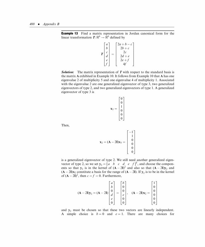
Example 13 Find a matrix representation in Jordan canonical form for the
linear transformation T: R6 ! R6 defined by
T
a
b
c
d
e
f
26666664
37777775 ¼
2aþ b� c
2bþ c
2c
2d þ e
2eþ f
4f
26666664
37777775
Solution: The matrix representation of T with respect to the standard basis is
the matrix A exhibited in Example 10. It follows from Example 10 that A has one
eigenvalue 2 of multiplicity 5 and one eigenvalue 4 of multiplicity 1. Associated
with the eigenvalue 2 are one generalized eigenvector of type 3, two generalized
eigenvectors of type 2, and two generalized eigenvectors of type 1. A generalized
eigenvector of type 3 is
x3 ¼
0
0
1
0
0
0
26666664
37777775
Then,
x2 ¼ (A� 2I)x3 ¼
�1
1
0
0
0
0
26666664
37777775
is a generalized eigenvector of type 2. We still need another generalized eigen-
vector of type 2, so we set y2 ¼ [ a b c d e f ]T, and choose the compon-
ents so that y2 is in the kernel of (A� 2I)2 and also so that (A� 2I)y2 and
(A� 2I)x2 constitute a basis for the range of (A� 2I). If y2 is to be in the kernel
of (A� 2I)2, then c ¼ f ¼ 0. Furthermore,
(A� 2I)y2 ¼ (A� 2I)
a
b
0
d
e
0
26666664
37777775 ¼
b
0
0
e
0
0
26666664
37777775, (A� 2I)x2 ¼
1
0
0
0
0
0
26666664
37777775
and y2 must be chosen so that these two vectors are linearly independent.
A simple choice is b ¼ 0 and e ¼ 1. There are many choices for
400 . Appendix B

y2 ¼ [ a 0 0 d 1 0 ]T, depending how a and d are selected. The simplest is
to take a ¼ d ¼ 0, whereupon
y2 ¼
0
0
0
0
1
0
26666664
37777775
Next,
y1 ¼ (A� 2I)y2 ¼
0
0
0
1
0
0
26666664
37777775 and x1 ¼ (A� 2I)x2 ¼
1
0
0
0
0
0
26666664
37777775
are the required generalized eigenvectors of type 1. There is only one linearly
independent generalized eigenvector associated with the eigenvalue 4. A suitable
candidate is
z1 ¼
0
0
0
1
2
4
26666664
37777775
We take our canonical basis to be fz1, y1, y2, x1, x2, x3g. With respect to this
basis, T is represented by the matrix in Jordan canonical form
J ¼
4 0 0 0 0 0
0 2 1 0 0 0
0 0 2 0 0 0
0 0 0 2 1 0
0 0 0 0 2 1
0 0 0 0 0 2
26666664
37777775 &
The Jordan canonical form found in Example 13 contained a 1� 1 Jordan block
with the eigenvalue 4 on the main diagonal, a 2� 2 Jordan block with the
eigenvalue 2 on the main diagonal, and a 3� 3 Jordan block again with the
eigenvalue 2 on the main diagonal. The 1� 1 Jordan block corresponds to the
single element chain z1 in the canonical basis, the 2� 2 Jordan block corres-
ponds to the two element chain y1, y2 in the canonical basis, while the 3� 3
Jordan block corresponds to the three element chain in the canonical basis. If we
rearrange the ordering of the chains in the canonical basis, then the Jordan
Jordan Canonical Forms . 401

blocks in the Jordan canonical form will be rearranged in a corresponding
manner. In particular, if we take the canonical basis to be fx1, x2, x3, y1, y2, z1g,then the corresponding Jordan canonical form becomes
J ¼
2 1 0 0 0 0
0 2 1 0 0 0
0 0 2 0 0 0
0 0 0 2 1 0
0 0 0 0 2 0
0 0 0 0 0 4
26666664
37777775
If, instead, we take the ordering of the canonical basis to be fx1, x2, x3, z1, y1, y2g,then the corresponding Jordan canonical form becomes
J ¼
2 1 1 0 0 0
0 2 1 0 0 0
0 0 2 0 0 0
0 0 0 4 0 0
0 0 0 0 2 1
0 0 0 0 0 2
26666664
37777775
Two criteria must be observed if a canonical basis is to generate a matrix in
Jordan canonical form. First, all vectors in the same chain must be grouped
together (not separated by vectors from other chains), and second, each chain
must be ordered by increasing type (so that the generalized eigenvector of type 1
appears before the generalized eigenvector of type 2 of the same chain, which
appears before the generalized eigenvector of type 3 of the same chain, and so
on). If either criterion is violated, then the ones will not appear, in general, on the
superdiagonal. In particular, if vectors are ordered by decreasing type, then all
the ones appear on the subdiagonal, the diagonal just below the main diagonal.
Let A denote a matrix representation of a linear transformation T: V! V with
respect to a basis B (perhaps the standard basis), and let J be a matrix represen-
tation in Jordan canonical form for T. J is the matrix representation with respect
to a canonical basis C. Since J and A are two matrix representations of the same
linear transformation, with respect to different basis, they must be similar. Using
the notation developed in Section 3.4 (see, in particular, Eq. (3.26) in that
section), we may write
JCC ¼ PB
C
)�1AB
BPBC (B:19)
where PBC is the transition matrix from the B basis to the C basis.
Let fx1, x2, . . . , xng be a canonical basis of generalized eigenvectors for A. A
generalized modal matrix is a matrix M whose columns are the vectors in the
canonical basis, that is,
In a canonical basis,
all vectors from the
same chain are
grouped together,
and generalized
eigenvectors in each
chain are ordered by
increasing type.
402 . Appendix B

M ¼ x1 x2 � � � xn½ � (B:20)
If xjþ1 is a direct ancestor of xj in the same chain corresponding to the eigenvalue
l, then
Axjþ1 ¼ lxjþ1 þ xj (B:10 repeated)
If x1 is an eigenvector corresponding to l, then
Ax1 ¼ lx1 (B:11 repeated)
Using these relationships, it is a simple matter to show that AM ¼MJ. Since the
columns of M are linearly independent, M has an inverse. Therefore,
J ¼M�1AM (B:21)
A ¼MJM�1 (B:22)
Comparing (B.21) with (B.19), we see that the generalized modal matrix is just
the transition matrix from the canonical basis C to the B basis. It then follows
that M�1 is the transition matrix from the B basis to the C basis.
Problems Appendix B
(1) Let L: R2 ! R2 be defined by Ta
b
� �¼ aþ 2b
4aþ 3b
� �:Determine whether the subspaces
spanned by the following sets of vectors are invariant subspaces of L.
(a) A ¼ 1
1
� �,
1
�1
� � �; (b) B ¼ 1
1
� �,�1
�1
� � �;
(c) C ¼ 2
1
� � �; (d) D ¼ 1
2
� � �;
(e) E ¼ 0
0
� � �; (f) F ¼ 0
0
� �,
1
�1
� � �:
(2) Let T: R3 ! R3 be defined by T
a
b
c
2435 ¼ 4bþ 2c
�3aþ 8bþ 3c
4a� 8b� 2c
24
35: Determine whether the
subspaces spanned by the following sets of vectors are invariant subspaces of T.
(a) A ¼2
1
0
2435,
2
3
�4
24
35
8<:
9=;; (b) B ¼
0
�2
4
24
35,
4
4
�4
24
35
8<:
9=;;
Jordan Canonical Forms . 403

ðcÞ C ¼2
1
0
2435,
0
0
1
2435
8<:
9=;; ðdÞ D ¼
0
0
1
2435,
2
3
�4
24
35
8<:
9=;;
ðeÞ E ¼0
0
1
2435
8<:
9=;; ðfÞ F ¼
2
3
�4
24
35
8<:
9=;:
(3) Let R: R4 ! R4 be defined by T
a
b
c
d
2664
3775 ¼
2aþ b� d
2bþ cþ d
2c
2d
2664
3775: Determine whether the
subspaces spanned by the following sets of vectors are invariant subspaces of R.
(a)
1
0
0
0
26643775,
�1
1
0
0
2664
3775
8>><>>:
9>>=>>;; (b)
1
0
0
0
26643775,
0
0
0
1
26643775
8>><>>:
9>>=>>;;
(c)
1
0
0
0
26643775,
0
�1
1
�1
2664
3775
8>><>>:
9>>=>>;; (d)
0
0
0
1
26643775,
0
�1
1
�1
2664
3775
8>><>>:
9>>=>>;;
(e)
1
0
0
0
26643775,
�1
1
0
0
2664
3775,
0
0
0
1
26643775
8>><>>:
9>>=>>;; (f)
1
0
0
0
26643775,
�1
1
0
0
2664
3775,
0
�1
1
�1
2664
3775
8>><>>:
9>>=>>;:
(4) Determine whether the subspaces spanned by the following sets of vectors are
invariant subspaces of A ¼ 3 1
�1 5
� �:
(a) A ¼ 0
1
� � �; (b) B ¼ 1
1
� � �;
(c) C ¼ 1
2
� � �; (d) D ¼ 1
1
� �,
0
1
� � �;
(e) E ¼ 1
1
� �,
2
2
� � �; (f) F ¼ 1
1
� �,
1
2
� � �:
(5) Determine whether the subspaces spanned by the following sets of vectors are
invariant subspaces of A ¼5 1 �1
0 5 2
0 0 5
24
35:
404 . Appendix B
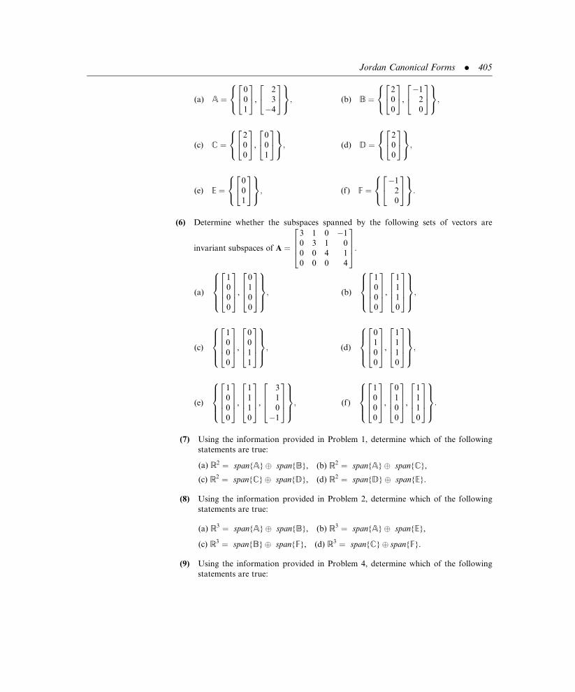
(a) A ¼0
0
1
2435,
2
3
�4
24
35
8<:
9=;; (b) B ¼
2
0
0
2435,
�1
2
0
24
35
8<:
9=;;
(c) C ¼2
0
0
2435,
0
0
1
2435
8<:
9=;; (d) D ¼
2
0
0
2435
8<:
9=;;
(e) E ¼0
0
1
2435
8<:
9=;; (f) F ¼
�1
2
0
24
35
8<:
9=;:
(6) Determine whether the subspaces spanned by the following sets of vectors are
invariant subspaces of A ¼
3 1 0 �1
0 3 1 0
0 0 4 1
0 0 0 4
2664
3775:
(a)
1
0
0
0
26643775,
0
1
0
0
26643775
8>><>>:
9>>=>>;; (b)
1
0
0
0
26643775,
1
1
1
0
26643775
8>><>>:
9>>=>>;;
(c)
1
0
0
0
26643775,
0
0
1
1
26643775
8>><>>:
9>>=>>;; (d)
0
1
0
0
26643775,
1
1
1
0
26643775
8>><>>:
9>>=>>;;
(e)
1
0
0
0
26643775,
1
1
1
0
26643775,
3
1
0
�1
2664
3775
8>><>>:
9>>=>>;; (f)
1
0
0
0
26643775,
0
1
0
0
26643775,
1
1
1
0
26643775
8>><>>:
9>>=>>;:
(7) Using the information provided in Problem 1, determine which of the following
statements are true:
(a) R2 ¼ span{A}� span{B}, (b) R2 ¼ span{A}� span{C},
(c) R2 ¼ span{C}� span{D}, (d) R2 ¼ span{D}� span{E}.
(8) Using the information provided in Problem 2, determine which of the following
statements are true:
(a) R3 ¼ span{A}� span{B}, (b) R3 ¼ span{A}� span{E},
(c) R3 ¼ span{B}� span{F}, (d) R3 ¼ span{C}� span{F}.
(9) Using the information provided in Problem 4, determine which of the following
statements are true:
Jordan Canonical Forms . 405

(a) R2 ¼ span{A}� span{B}, (b) R2 ¼ span{A}� span{C},
(c) R2 ¼ span{B}� span{C}, (d) R2 ¼ span{E}� span{F}.
(10) Using the information provided in Problem 5, determine which of the following
statements are true:
(a) R3 ¼ span{A}� span{D}, (b) R3 ¼ span{B}� span{D},
(c) R3 ¼ span{B}� span{E}, (d) R3 ¼ span{D}� span{E}.
(11) Characterize the subspace U ¼ span{D}� span{E} for the sets D and E described
in Problem 5.
(12) Let T: R4 ! R4 be defined by T
a
b
c
d
2664
3775 ¼
3aþ b� d
3bþ c
4cþ d
4d
2664
3775: Set B ¼
1
1
0
0
26643775,
1
�1
0
0
2664
3775
8>><>>:
9>>=>>;,
C ¼
�1
�1
�1
0
2664
3775,
3
1
0
�1
2664
3775
8>><>>:
9>>=>>;, M ¼ span (B); and N ¼ span (C):
(a) Show that M and N are both invariant subspaces of T with R4 ¼M�N.
(b) Show that T has a matrix representation in the block diagonal form with respect
to the basis B [ C.
(13) Let T: R4 ! R4 be defined by T
a
b
c
d
2664
3775 ¼
2aþ b� d
2bþ cþ d
2c
2d
2664
3775: Set B ¼
0
1
�1
1
2664
3775
8>><>>:
9>>=>>;,
C ¼
1
1
0
0
26643775,
1
�1
0
0
2664
3775,
0
0
0
1
26643775
8>><>>:
9>>=>>;, M ¼ span (B); and N ¼ span (C):
8>><>>:
(a) Show that M and N are both invariant subspaces of T with R4 ¼M�N.
(b) Show that T has a matrix representation in the block diagonal form with
respect to the basis B [ C.
(14) Let T: R4 ! R4 be defined by T
a
b
c
d
26643775 ¼
4aþ c
2aþ 2bþ 3c
�aþ 2c
4aþ cþ 2d
2664
3775: Set B ¼
0
1
0
1
26643775,
0
0
0
1
26643775
8>><>>:
9>>=>>;,
C ¼
1
�1
�1
3
2664
3775,
1
3
0
1
26643775
8>><>>:
9>>=>>;, M ¼ span (B); and N ¼ span (C):
(a) Show that M and N are both invariant subspaces of T with R4 ¼M�N.
(b) Show that T has a matrix representation in the block diagonal form with
respect to the basis B [ C.
406 . Appendix B

(15) Determine whether the following vectors are generalized eigenvectors of type 3
corresponding to the eigenvalue l ¼ 2 for the matrix
A ¼
2 2 1 1
0 2 �1 0
0 0 2 0
0 0 0 1
2664
3775
(a)
1
1
1
0
26643775, (b)
0
1
0
0
26643775, (c)
0
0
1
0
26643775, (d)
2
0
3
0
26643775, (e)
0
0
0
1
26643775, (f)
0
0
0
0
26643775:
For the matrices in Problems 16 through 20, find a generalized eigenvector of type 2
corresponding the eigenvalue l ¼ �1.
(16)�1 1
0 �1
� �: (17)
�1 1 0
0 �1 1
0 0 1
24
35: (18)
0 4 2
�1 4 1
�1 �7 �4
24
35:
(19)
3 �2 2
2 �2 1
�9 9 �4
24
35: (20)
2 0 3
2 �1 1
�1 0 �2
24
35:
(21) Find a generalized eigenvector of type 3 corresponding to l ¼ 3 and a generalized
eigenvector of type 2 corresponding to l ¼ 4 for
A ¼
4 1 0 0 1
0 4 0 0 0
0 0 3 1 0
0 0 0 3 2
0 0 0 0 3
266664
377775:
(22) The vector [1 1 1 0]T is known to be a generalized eigenvector of type 3
corresponding to the eigenvalue 2 for
A ¼
2 2 1 1
0 2 �1 0
0 0 2 0
0 0 0 1
2664
3775
Construct a chain from this vector.
(23) Redo Problem 22 for the generalized eigenvector [0 0 1 0]T, which is also of
type 3 corresponding to the same eigenvalue and matrix.
(24) The vector [ 0 0 0 0 1]T is known to be a generalized eigenvector of type 4
corresponding to the eigenvalue 1 for
A ¼
1 0 1 0 �1
0 1 0 0 0
0 0 1 �1 2
0 0 0 1 1
0 0 0 0 1
266664
377775
Construct a chain from this vector.
Jordan Canonical Forms . 407

(25) Redo Problem 24 for the generalized eigenvector [ 0 0 0 1 0]T , which is of
type 3 corresponding to the same eigenvalue and matrix.
(26) The vector [ 1 0 0 0 �1]T is known to be a generalized eigenvector of type 3
corresponding to the eigenvalue 3 for
A ¼
4 1 0 0 1
0 4 0 0 0
0 0 3 1 0
0 0 0 3 2
0 0 0 0 3
266664
377775
Construct a chain from this vector.
(27) Redo Problem 26 for the generalized eigenvector [ 0 1 0 0 0]T , which is of
type 2 corresponding to the eigenvalue 4 for the same matrix.
(28) Find a generalized eigenvector of type 2 corresponding to the eigenvalue �1 for
A ¼ �1 1
0 �1
� �
and construct a chain from this vector.
(29) Find a generalized eigenvector of type 2 corresponding to the eigenvalue �1 for
A ¼�1 1 0
0 �1 1
0 0 1
24
35
and construct a chain from this vector.
(30) Find a generalized eigenvector of type 2 corresponding to the eigenvalue �1 for
A ¼0 4 2
�1 4 1
�1 �7 �4
24
35
and construct a chain from this vector.
(31) Find a generalized eigenvector of type 4 corresponding to the eigenvalue 2 for
A ¼
2 1 3 �1
0 2 �1 4
0 0 2 1
0 0 0 2
2664
3775
and construct a chain from this vector.
(32) Find a generalized eigenvector of type 3 corresponding to the eigenvalue 3 for
A ¼
4 1 1 2 2
�1 2 1 3 0
0 0 3 0 0
0 0 0 2 1
0 0 0 1 2
266664
377775
and construct a chain from this vector.
408 . Appendix B

(33) Prove that a generalized eigenvector of type 1 is an eigenvector.
(34) Prove that a generalized eigenvector of any type cannot be a zero vector.
(35) Let T: V! V be a linear transformation. Prove that the following sets are invariant
subspaces under T.
(a) {0}, (b) V;
(c) span{v1, v2, . . . , vk} where each vector is an eigenvector of T (not necessarily
corresponding to the same eigenvalue).
(36) Let V be a finite-dimensional vector space. Prove that V is the direct sum of two
subspaces U and W if and only if (i) each vector in V can be written as the sum of a
vector in U with a vector in W, and (ii) the only vector common to both U and W is
the zero vector.
(37) Let B be a basis of k-vectors for U, an invariant subspace of the linear transform-
ation T: V! V, and let C be a basis for W, another subspace (but not invariant)
with V ¼ U�W. Show that the matrix representation of T with respect to the basis
B [ C has the partitioned form
A ¼ A1 A2
0 A3
� �
with A1 having order k� k.
(38) Determine the length of the chains in a canonical basis if each chain is associated
with the same eigenvalue l and if a full set of index numbers is given by each of the
following.
(a) r3 ¼ r2 ¼ r1 ¼ 1, (b) r3 ¼ r2 ¼ r1 ¼ 2,
(c) r3 ¼ 1, r2 ¼ r1 ¼ 2, (d) r3 ¼ 1, r2 ¼ 2, r1 ¼ 3,
(e) r3 ¼ r2 ¼ 1, r1 ¼ 3, (f) r3 ¼ 3, r2 ¼ 4, r1 ¼ 3,
(g) r2 ¼ 2, r1 ¼ 4, (h) r2 ¼ 4, r1 ¼ 2,
(i) r2 ¼ 2, r1 ¼ 3, (j) r2 ¼ r1 ¼ 2.
In Problems 39 through 45, find a canonical basis for the given matrices.
(39)3 1
�1 1
� �. (40)
7 3 3
0 1 0
�3 �3 1
24
35.
(41)
5 1 �1
0 5 2
0 0 5
24
35. (42)
5 1 2
0 3 0
2 1 5
24
35.
(43)
2 1 0 �1
0 2 1 1
0 0 2 0
0 0 0 2
2664
3775. (44)
3 1 0 �1
0 3 1 0
0 0 4 1
0 0 0 4
2664
3775.
Jordan Canonical Forms . 409

(45)
4 1 1 0 0 �1
0 4 2 0 0 1
0 0 4 1 0 0
0 0 0 5 1 0
0 0 0 0 5 2
0 0 0 0 0 4
26666664
37777775.
In Problems 46 through 50, a full set of index numbers are specified for the eigenvalue 2 of
multiplicity 5 for a 5� 5 matrix A. In each case, find a matrix in Jordan canonical form
that is similar to A. Assume that a canonical basis is ordered so that chains of length 1
appear before chains of length 2, which appear before chains of length 3, and so on.
(46) r3 ¼ r2 ¼ 1, r1 ¼ 3. (47) r3 ¼ 1, r2 ¼ r1 ¼ 2.
(48) r2 ¼ 2, r1 ¼ 3. (49) r4 ¼ r3 ¼ r2 ¼ 1, r1 ¼ 2.
(50) r5 ¼ r4 ¼ r3 ¼ r2 ¼ r1 ¼ 1.
In Problems 51 through 56, a full set of index numbers are specified for the eigenvalue 3 of
multiplicity 6 for a 6� 6 matrix A. In each case, find a matrix in Jordan canonical form
that is similar to A. Assume that a canonical basis is ordered so that chains of length 1
appear before chains of length 2, which appear before chains of length 3, and so on.
(51) r3 ¼ r2 ¼ r1 ¼ 2. (52) r3 ¼ 1, r2 ¼ 2, r1 ¼ 3.
(53) r3 ¼ r2 ¼ 1, r1 ¼ 4. (54) r2 ¼ r1 ¼ 3.
(55) r2 ¼ 2, r1 ¼ 4. (56) r2 ¼ 1, r1 ¼ 5.
(57) A canonical basis for a linear transformation T: R4 ! R4 contains three chains
corresponding to the eigenvalue 2: two chains x1 and y1, each of length 1, and one
chain w1,w2 of length 2. Find the matrix representation of T with respect to this
canonical basis, ordered as follows.
(a) fx1, y1,w1,w2g, (b) fy1,w1, w2, x1g,(c) fw1,w2, x1, y1g, (d) fw1,w2, y1, x1g.
(58) A canonical basis for a linear transformation T: R6 ! R6 contains two chains
corresponding to the eigenvalue 3: one chain x1 of length 1 and one chain y1, y2
of length 2, and two chains corresponding to the eigenvalue 5: one chain u1 of
length 1 and one chain of v1, v2 of length 2. Find the matrix representation of T with
respect to this canonical basis, ordered as follows.
(a) fx1, y1, y2, u1, v1, v2g, (b) fy1, y2, x1, u1, v1, v2g,(c) fx1, u1, v1, v2, y1, y2g, (d) fy1, y2, v1, v2, x1, u1g,(e) fx1, u1, y1, y2, v1, v2g, (f) fv1, v2, u1, v1, y1, y2g.
In Problems 59 through 73, find a matrix representation in Jordan canonical form for the
given linear transformation.
(59) Ta
b
� �¼ 2a� 3b
a� 2b
� �. (60) T
a
b
� �¼ 3aþ b
�aþ 5b
� �.
(61) Ta
b
� �¼ 2a� b
aþ 4b
� �. (62) T
a
b
� �¼ aþ 2b
�aþ 4b
� �.
410 . Appendix B

(63) Ta
b
� �¼ 2aþ b
2aþ 3b
� �. (64) T
a
b
� �¼ 2a� 5b
a� 2b
� �.
(65) T
a
b
c
2435 ¼ 9aþ 3bþ 3c
3b
�3a� 3bþ 3c
24
35. (66) T
a
b
c
2435 ¼ 2aþ 2b� 2c
2bþ c
2c
24
35.
(67) T
a
b
c
2435 ¼ bþ 2c
�2b
2aþ b
24
35. (68) T
a
b
c
2435 ¼ 2a� c
2aþ b� 2c
�aþ 2c
24
35.
(69) T
a
b
c
2435 ¼ aþ b� c
0
aþ 2bþ 3c
24
35. (70) T
a
b
c
2435 ¼ aþ 2bþ 3c
2aþ 4bþ 6c
3aþ 6bþ 9c
24
35.
(71) T
a
b
c
d
2664
3775 ¼
3aþ b� d
3bþ cþ d
3c
3d
2664
3775. (72) T
a
b
c
d
2664
3775 ¼
aþ b� d
bþ c
2cþ d
2d
2664
3775.
(73) T
a
b
c
d
e
f
g
2666666664
3777777775¼
�a� cþ d þ eþ 3f
b
2aþ bþ 2c� d � e� 6f
�2a� cþ 2d þ eþ 3f
e
f
�a� bþ d þ 2eþ 4f þ g
2666666664
3777777775, with l ¼ 1 as the only eigenvalue.
(74) The generalized null space of an n� n matrix A and eigenvalue l, denoted by Nl(A),
is the set of all vectors x 2 Rn such that (A� lI)kx ¼ 0 for some nonnegative
integer k. Show that if x is a generalized eigenvector of any type corresponding to
l, then x 2 Nl(A).
(75) Prove that Nl(A), as defined in Problem 74, is a subspace of Rn.
(76) Prove that every square matrix A commutes with (A� lI)n for every positive
integer n and every scalar l.
(77) Prove that Nl(A) is an invariant subspace of Rn under A.
(78) Prove that if A has order n� n and x 2 Nl(A), then (A� lI)nx ¼ 0.
Jordan Canonical Forms . 411

This page intentionally left blank

Appendix C
Markov Chains
Eigenvalues and eigenvectors arise naturally in the study of matrix representa-
tions of linear transformations, but that is far from their only use. In this
Appendix, we present an application to those probabilistic systems known as
Markov chains.
An elementary understanding of Markov chains requires only a little knowledge
of probabilities; in particular, that probabilities describe the likelihoods of
different events occurring, that probabilities are numbers between 0 and 1, and
that if the set of all possible events is limited to a finite number that are mutually
exclusive then the sum of the probabilities of each event occurring is 1. Signifi-
cantly more probability theory is needed to prove the relevant theorems about
Markov chains, so we limit ourselves in this section to simply understanding the
application.
" Definition 1. A finite Markov chain is a set of objects (perhaps
people), a set of consecutive time periods (perhaps five-year intervals),
and a finite set of different states (perhaps employed and unemployed)
such that
(i) during any given time period, each object is in only
one state (although different objects can be in differ-
ent states), and
(ii) the probability that an object will move from one
state to another state (or remain in the same state)
over a time period depends only on the beginning and
ending states. 3
We denote the states as state 1, state 2, state 3, through state N, and let pij
designate the probability of moving in one time period into state i from state
j(i, j ¼ 1, 2, . . . , N). The matrix P ¼ [pij ] is called a transition matrix.
413

Example 1
Construct a transition matrix for the following Markov chain. A traffic control
administrator in the Midwest classifies each day as either clear or cloudy.
Historical data show that the probability of a clear day following a cloudy day
is 0.6, whereas the probability of a clear day following a clear day is 0.9.
Solution: Although one can conceive of many other classifications such as
rainy, very cloudy, partly sunny, and so on, this particular administrator opted
for only two, so we have just two states: clear and cloudy, and each day must fall
into one and only one of these two states. Arbitrarily we take clear to be state 1
and cloudy to be state 2. The natural time unit is one day. We are given that
p12 ¼ 0:6, so it must follow that p22 ¼ 0:4, because after a cloudy day the next
day must be either clear or cloudy and the probability that one or the other of
these two events occurring is 1. Similarly, we are given that p11 ¼ 0:9, so it also
follows that p21 ¼ 0:1. The transition matrix is
clear cloudy
P ¼0:9 0:6
0:1 0:4
� �clear
cloudy &
Example 2
Construct a transition matrix for the following Markov chain. A medical survey
lists individuals as thin, normal, or obese. A review of yearly check-ups from
doctors’ records showed that 80% of all thin people remained thin one year later
while the other 20% gained enough weight to be reclassified as normal. For
individuals of normal weight, 10% became thin, 60% remained normal, and 30%
became obese the following year. Of all obese people, 90% remained obese one
year later while the other 10% lost sufficient weight to fall into the normal range.
Although some thin people became obese a year later, and vice versa, their
numbers were insignificant when rounded to two decimals.
Solution: We take state 1 to be thin, state 2 to be normal, and state 3 to be
obese. One time period equals one year. Converting each percent to its decimal
representation so that it may also represent a probability, we have p21 ¼ 0:2, the
probability of an individual having normal weight after being thin the previous
year, p32 ¼ 0:3, the probability of an individual becoming obese one year after
having a normal weight, and, in general,
thin normal obese
P ¼0:8 0:1 0
0:2 0:6 0:1
0 0:3 0:9
264
375 thin
normal &
obese
A transition matrix
for an N-state
Markov chain is an
N �N matrix with
nonnegative entries;
the sum of the
entries in each
column is 1.
414 . Appendix C

Powers of a transition matrix have the same properties of a transition matrix: all
elements are between 0 and 1, and every column sum equals 1 (see Problem 20).
Furthermore,
" Theorem 1. If P is a transition matrix for a finite Markov chain, and if
p(k)ij denotes the i-j element of P k, the kth power of P, then p
(k)ij is the
probability of moving to state i from state j in k time periods. 3
For the transition matrix created in Example 2, we calculate the second and third
powers as
thin normal obese
P2 ¼0:66 0:14 0:01
0:28 0:41 0:15
0:06 0:45 0:84
264
375 thin
normal
obese
and
thin normal obese
P3 ¼0:556 0:153 0:023
0:306 0:319 0:176
0:138 0:528 0:801
264
375 thin
normal &
obese
Here p(2)11 5 ¼ 0:66 is the probability of a thin person remaining thin two
years later, p(2)32 6 ¼ 0:45 is the probability of a normal person becoming fat
two years later, while p(2)13 7 ¼ 0:023 is the probability of a fat person becoming
thin three years later.
For the transition matrix created in Example 1, we calculate the second power
to be
clear cloudy
P2 ¼0:87 0:78
0:13 0:22
� �clear
cloudy
Consequently, p(2)12 9 ¼ 0:78 is the probability of a cloudy day being followed by
a clear day two days later, while p(2)22 10 ¼ 0:22 is the probability of a cloudy day
being followed by a cloudy day two days later. Calculating the tenth power of
this same transition matrix and rounding all entries to four decimal places for
presentation purposes, we have
clear cloudy
P10 ¼0:8571 0:8571
0:1429 0:1429
� �clear
cloudy
(C:1)
Markov Chains . 415

Since p(10)11 12 ¼ p
(10)12 13 ¼ 0:8571, it follows that the probability of having a clear
day 10 days after a cloudy day is the same as the probability of having a clear day
10 days after a clear day.
An object in a Markov chain must be in one and only one state at any time, but
that state is not always known with certainty. Often, probabilities are provided
to describe the likelihood of an object being in any one of the states at any given
time. These probabilities can be combined into an n-tuple. A distribution vector d
for an N-state Markov chain at a given time is an N-dimensional column matrix
having as its components, one for each state, the probabilities that an object in
the system is in each of the respective states at that time.
Example 3 Find the distribution vector for the Markov chain described in
Example 1 if the current day is known to be cloudy.
Solution: The objects in the system are days, which are classified as either clear,
state 1, or cloudy, state 2. We are told with certainty that the current day is
cloudy, so the probability that the day is cloudy is 1 and the probability that the
day is clear is 0. Therefore,
d ¼ 0
1
� �&
Example 4 Find the distribution vector for the Markov chain described in
Example 2 if it is known that currently 7% of the population is thin, 31% of
population is of normal weight, and 62% of the population is obese.
Solution: The objects in the system are people. Converting the stated percentages
into their decimal representations, we have
d ¼0:07
0:31
0:62
24
35 &
Different time periods can have different distribution vectors, so we let d(k)
denote a distribution vector after k time periods. In particular, d(1) is a distribu-
tion vector after 1 time period, d(2) is a distribution vector after 2 time periods,
and d(10) is a distribution vector after 10 time periods. An initial distribution
vector for the beginning of a Markov chain is designated by d(0). The distribution
vectors for various time periods are related.
" Theorem 2. If P is a transition matrix for a Markov chain, then
d(k) ¼ Pkd(0) ¼ Pd(k�1),
where Pk denotes the kth power of P. 3
A distribution
vector for an N-state
Markov chain at a
given time is a
column matrix
whose i th
component is the
probability that an
object is in the ith
state at that given
time.
416 . Appendix C
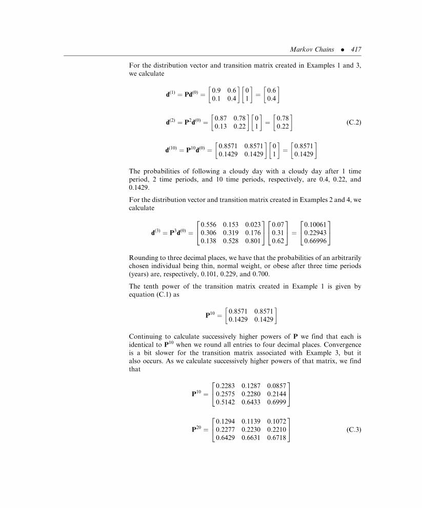
For the distribution vector and transition matrix created in Examples 1 and 3,
we calculate
d(1) ¼ Pd(0) ¼ 0:9 0:60:1 0:4
� �0
1
� �¼ 0:6
0:4
� �
d(2) ¼ P2d(0) ¼ 0:87 0:78
0:13 0:22
� �0
1
� �¼ 0:78
0:22
� �(C:2)
d(10) ¼ P10d(0) ¼ 0:8571 0:8571
0:1429 0:1429
� �0
1
� �¼ 0:8571
0:1429
� �
The probabilities of following a cloudy day with a cloudy day after 1 time
period, 2 time periods, and 10 time periods, respectively, are 0.4, 0.22, and
0.1429.
For the distribution vector and transition matrix created in Examples 2 and 4, we
calculate
d(3) ¼ P3d(0) ¼0:556 0:153 0:023
0:306 0:319 0:176
0:138 0:528 0:801
24
35 0:07
0:31
0:62
24
35 ¼ 0:10061
0:22943
0:66996
24
35
Rounding to three decimal places, we have that the probabilities of an arbitrarily
chosen individual being thin, normal weight, or obese after three time periods
(years) are, respectively, 0.101, 0.229, and 0.700.
The tenth power of the transition matrix created in Example 1 is given by
equation (C.1) as
P10 ¼ 0:8571 0:8571
0:1429 0:1429
� �
Continuing to calculate successively higher powers of P we find that each is
identical to P10 when we round all entries to four decimal places. Convergence
is a bit slower for the transition matrix associated with Example 3, but it
also occurs. As we calculate successively higher powers of that matrix, we find
that
P10 ¼0:2283 0:1287 0:0857
0:2575 0:2280 0:2144
0:5142 0:6433 0:6999
24
35
P20 ¼0:1294 0:1139 0:1072
0:2277 0:2230 0:2210
0:6429 0:6631 0:6718
24
35 (C:3)
Markov Chains . 417
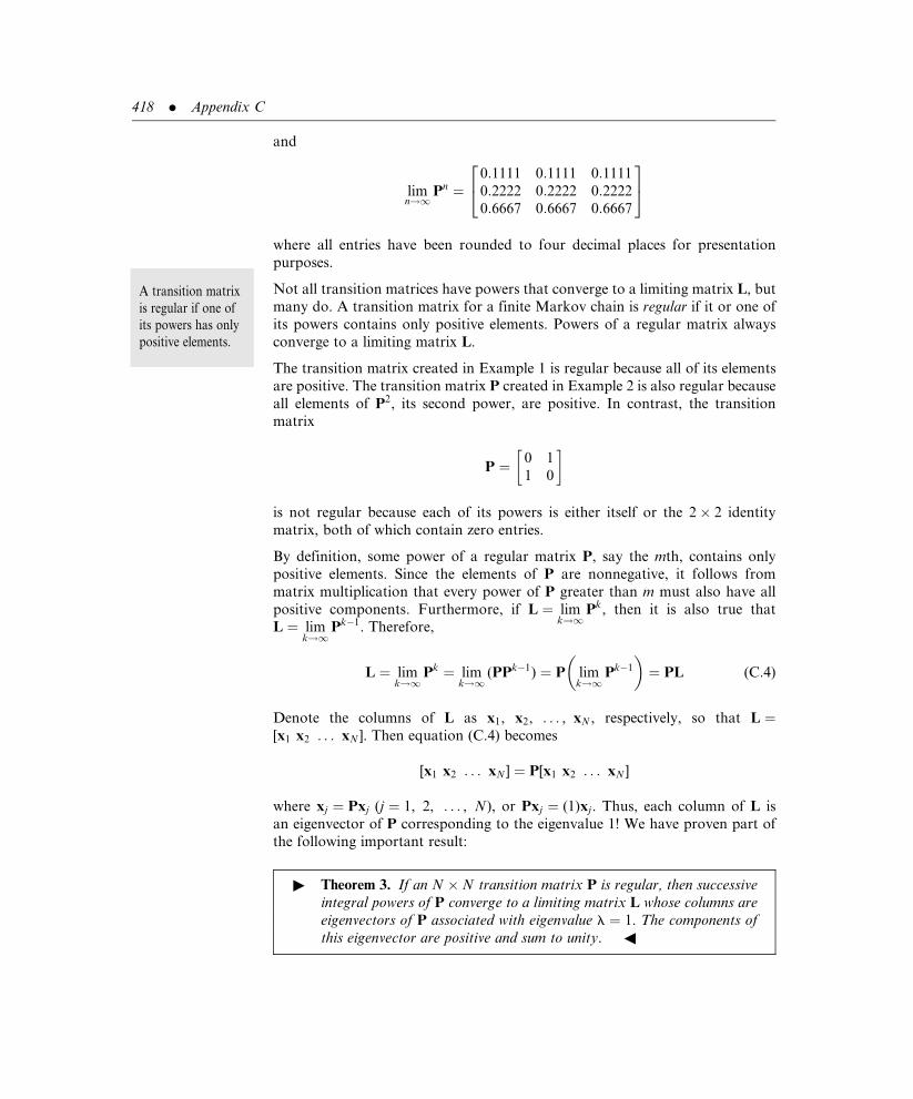
and
limn!1
Pn ¼0:1111 0:1111 0:1111
0:2222 0:2222 0:2222
0:6667 0:6667 0:6667
24
35
where all entries have been rounded to four decimal places for presentation
purposes.
Not all transition matrices have powers that converge to a limiting matrix L, but
many do. A transition matrix for a finite Markov chain is regular if it or one of
its powers contains only positive elements. Powers of a regular matrix always
converge to a limiting matrix L.
The transition matrix created in Example 1 is regular because all of its elements
are positive. The transition matrix P created in Example 2 is also regular because
all elements of P2, its second power, are positive. In contrast, the transition
matrix
P ¼ 0 1
1 0
� �
is not regular because each of its powers is either itself or the 2� 2 identity
matrix, both of which contain zero entries.
By definition, some power of a regular matrix P, say the mth, contains only
positive elements. Since the elements of P are nonnegative, it follows from
matrix multiplication that every power of P greater than m must also have all
positive components. Furthermore, if L ¼ limk!1
Pk, then it is also true that
L ¼ limk!1
Pk�1. Therefore,
L ¼ limk!1
Pk ¼ limk!1
(PPk�1) ¼ P limk!1
Pk�1
� �¼ PL (C:4)
Denote the columns of L as x1, x2, . . . , xN , respectively, so that L ¼[x1 x2 . . . xN ]. Then equation (C.4) becomes
[x1 x2 . . . xN ] ¼ P[x1 x2 . . . xN ]
where xj ¼ Pxj (j ¼ 1, 2, . . . , N), or Pxj ¼ (1)xj. Thus, each column of L is
an eigenvector of P corresponding to the eigenvalue 1! We have proven part of
the following important result:
" Theorem 3. If an N �N transition matrix P is regular, then successive
integral powers of P converge to a limiting matrix L whose columns are
eigenvectors of P associated with eigenvalue l ¼ 1. The components of
this eigenvector are positive and sum to unity. 3
A transition matrix
is regular if one of
its powers has only
positive elements.
418 . Appendix C

Even more is true. If P is regular, then its eigenvalue l ¼ 1 has multiplicity 1, and
there is only one linearly independent eigenvector associated with that eigen-
value. This eigenvector will be in terms of one arbitrary constant, which is
uniquely determined by the requirement that the sum of the components is 1.
Thus, each column of L is the same eigenvector.
We define the limiting state distribution vector for an N-state Markov chain as
an N-dimensional column vector d(1) having as its components the limiting
probabilities that an object in the system is in each of the respective states after
a large number of time periods. That is,
d(1) ¼ limn!1
d(n)
Consequently,
d(1) ¼ limn!1
d(n) ¼ limn!1
(P nd(0)) ¼ limn!1
P n� �
d(0) ¼ Ld(0)
Each column of L is identical to every other column, so each row of L contains
a single number repeated N times. Combining this with the fact that d(0) has
components that sum to 1, it follows that the product Ld(0) is equal to each of
the identical columns of L. That is, d(1) is the eigenvector of P corresponding to
l ¼ 1, having the sum of its components equal to 1.
Example 5 Find the limiting state distribution vector for the Markov chain
described in Example 1.
Solution: The transition matrix is
P ¼ 0:9 0:60:1 0:4
� �
which is regular. Eigenvectors for this matrix have the form
x ¼ x
y
� �
Eigenvectors corresponding to l ¼ 1 satisfy the matrix equation (P� 1I)x ¼ 0,
or equivalently, the set of equations
�0:1xþ 0:6y ¼ 00:1x� 0:6y ¼ 0
Solving by Gaussian elimination, we find x ¼ 6y with y arbitrary. Thus,
x ¼ 6y
y
� �
The limiting state
distribution vector
for a transition
matrix P is the
unique eigenvector
of P corresponding
to l ¼ 1, having
the sum of its
components equal
to 1.
Markov Chains . 419

If we choose y so that the sum of the components of x sum to 1, we have
7y ¼ 1, or y ¼ 1=7. The resulting eigenvector is the limiting state distribution
vector, namely
d(1) ¼ 6=71=7
� �
Furthermore,
L ¼ 6=7 6=71=7 1=7
� �
Over the long run, six out of seven days will be clear and one out of seven days
will be cloudy. We see from equations (C.1) and (C.2) that convergence to four
decimal places for the limiting state distribution and L is achieved after 10 time
periods. &
Example 6 Find the limiting state distribution vector for the Markov chain
described in Example 2.
Solution: The transition matrix is
P ¼0:8 0:1 0
0:2 0:6 0:10 0:3 0:9
24
35
P2 has only positive elements, so P is regular. Eigenvectors for this matrix have
the form
x ¼x
y
z
2435
Eigenvectors corresponding to l ¼ 1 satisfy the matrix equation (P� 1I)x ¼ 0,
or equivalently, the set of equations
�0:2xþ 0:1y ¼ 00:2x� 0:4yþ 0:1z ¼ 0
0:3y� 0:1z ¼ 0
Solving by Gaussian elimination, we find x ¼ (1=6)z, y ¼ (1=3)z, with z arbitrary.
Thus,
x ¼z=6z=3z
24
35
420 . Appendix C

We choose z so that the sum of the components of x sum to 1, hence
(1=6)zþ (1=3)zþ z ¼ 1, or z ¼ 2=3. The resulting eigenvector is the limiting
state distribution vector, namely,
d(1) ¼1=92=96=9
24
35
Furthermore,
L ¼1=9 1=9 1=92=9 2=9 2=96=9 6=9 6=9
24
35
Compare L with equation (C.3). The components of d(1) imply that, over the
long run, one out of nine people will be thin, two out of nine people will be of
normal weight, and six out of nine people will be obese. &
Problems Appendix C
(1) Determine which of the following matrices cannot be transition matrices and
explain why:
(a)0:15 0:57
0:85 0:43
� �, (b)
0:27 0:74
0:63 0:16
� �,
(c)0:45 0:53
0:65 0:57
� �, (d)
1:27 0:23
�0:27 0:77
� �,
(e)
1 1=2 0
0 1=3 0
0 1=6 0
24
35, (f)
1=2 1=2 1=31=4 1=3 1=41=4 1=6 7=12
24
35,
(g)
0:34 0:18 0:53
0:38 0:42 0:21
0:35 0:47 0:19
24
35, (h)
0:34 0:32 �0:17
0:78 0:65 0:80
�0:12 0:03 0:37
24
35:
(2) Construct a transition matrix for the following Markov chain: Census figures show
a population shift away from a large midwestern metropolitan city to its suburbs.
Each year, 5% of all families living in the city move to the suburbs while during the
same time period only 1% of those living in the suburbs move into the city. Hint:
Take state 1 to represent families living in the city, state 2 to represent families living
in the suburbs, and one year as one time period.
(3) Construct a transition matrix for the following Markov chain: Every four years,
voters in a New England town elect a new mayor because a town ordinance prohibits
mayors from succeeding themselves. Past data indicate that a Democratic mayor is
succeeded by another Democrat 30% of the time and by a Republican 70% of the
Markov Chains . 421

time. A Republican mayor, however, is succeeded by another Republican 60% of
the time and by a Democrat 40% of the time. Hint: Take state 1 to represent
a Republican mayor in office, state 2 to represent a Democratic mayor in office,
and four years as one time period.
(4) Construct a transition matrix for the following Markov chain: The apple harvest in
New York orchards is classified as poor, average, or good. Historical data indicates
that if the harvest is poor one year then there is a 40% chance of having a good
harvest the next year, a 50% chance of having an average harvest, and a 10% chance
of having another poor harvest. If a harvest is average one year, the chance of a poor,
average, or good harvest the next year is 20%, 60%, and 20%, respectively. If
a harvest is good, then the chance of a poor, average, or good harvest the next year
is 25%, 65%, and 10%, respectively. Hint: Take state 1 to be a poor harvest, state 2 to
be an average harvest, state 3 to be a good harvest, and one year as one time period.
(5) Construct a transition matrix for the following Markov chain: Brand X and brand
Y control the majority of the soap powder market in a particular region, and each
has promoted its own product extensively. As a result of past advertising campaigns,
it is known that over a two-year period of time, 10% of brand Y customers change
to brand X and 25% of all other customers change to brand X. Furthermore, 15%
of brand X customers change to brand Y and 30% of all other customers change
to brand Y. The major brands also lose customers to smaller competitors, with 5% of
brand X customers switching to a minor brand during a two-year time period and 2%
of brand Y customers doing likewise. All other customers remain loyal to their past
brand of soap powder. Hint: Take state 1 to be a brand X customer, state 2 a brand
Y customer, state 3 another brand’s customer, and two years as one time period.
(6) (a) Calculate P2 and P3 for the two-state transition matrix:
P ¼ 0:1 0:40:9 0:6
� �
(b) Determine the probability of an object beginning in state 1 and remaining in
state 1 after two time periods.
(c) Determine the probability of an object beginning in state 1 and ending in state 2
after two time periods.
(d) Determine the probability of an object beginning in state 1 and ending in state 2
after three time periods.
(e) Determine the probability of an object beginning in state 2 and remaining in
state 2 after three time periods.
(7) Consider a two-state Markov chain. List the number of ways an object in state 1 can
end in state 1 after three time periods.
(8) Consider the Markov chain described in Problem 2. Determine (a) the probability a
family living in the city will find themselves in the suburbs after two years, and (b) the
probability a family living in the suburbs will find themselves living in the city after
two years.
(9) Consider the Markov chain described in Problem 3. Determine (a) the probability
there will be a Republican mayor eight years after a Republican mayor serves, and
(b) the probability there will be a Republican mayor 12 years after a Republican
mayor serves.
422 . Appendix C
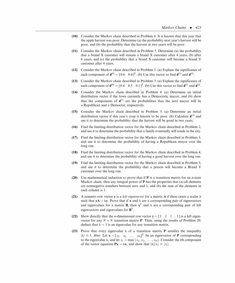
(10) Consider the Markov chain described in Problem 4. It is known that this year that
the apple harvest was poor. Determine (a) the probability next year’s harvest will be
poor, and (b) the probability that the harvest in two years will be poor.
(11) Consider the Markov chain described in Problem 5. Determine (a) the probability
that a brand X customer will remain a brand X customer after 4 years, (b) after
6 years, and (c) the probability that a brand X customer will become a brand Y
customer after 4 years.
(12) Consider the Markov chain described in Problem 2. (a) Explain the significance of
each component of d(0) ¼ [ 0:6 0:4 ]T. (b) Use this vector to find d(1) and d(2).
(13) Consider the Markov chain described in Problem 3. (a) Explain the significance of
each component of d(0) ¼ [ 0:4 0:5 0:1 ]T. (b) Use this vector to find d(1) and d(2).
(14) Consider the Markov chain described in Problem 4. (a) Determine an initial
distribution vector if the town currently has a Democratic mayor, and (b) show
that the components of d(1) are the probabilities that the next mayor will be
a Republican and a Democrat, respectively.
(15) Consider the Markov chain described in Problem 5. (a) Determine an initial
distribution vector if this year’s crop is known to be poor. (b) Calculate d(2) and
use it to determine the probability that the harvest will be good in two years.
(16) Find the limiting distribution vector for the Markov chain described in Problem 2,
and use it to determine the probability that a family eventually will reside in the city.
(17) Find the limiting distribution vector for the Markov chain described in Problem 3,
and use it to determine the probability of having a Republican mayor over the
long run.
(18) Find the limiting distribution vector for the Markov chain described in Problem 4,
and use it to determine the probability of having a good harvest over the long run.
(19) Find the limiting distribution vector for the Markov chain described in Problem 5,
and use it to determine the probability that a person will become a Brand Y
customer over the long run.
(20) Use mathematical induction to prove that if P is a transition matrix for an n-state
Markov chain, then any integral power of P has the properties that (a) all elements
are nonnegative numbers between zero and 1, and (b) the sum of the elements in
each column is 1.
(21) A nonzero row vector y is a left eigenvector for a matrix A if there exists a scalar l
such that yA ¼ ly. Prove that if x and l are a corresponding pair of eigenvectors
and eigenvalues for a matrix B, then xT and l are a corresponding pair of left
eigenvectors and eigenvalues for BT.
(22) Show directly that the n-dimensional row vector y ¼ [ 1 1 1 . . . 1 ] is a left eigen-
vector for any N �N transition matrix P. Then, using the results of Problem 20,
deduce that l ¼ 1 is an eigenvalue for any transition matrix.
(23) Prove that every eigenvalue l of a transition matrix P satisfies the inequality
jlj # 1. Hint: Let x ¼ [ x1 x2 . . . xN]T be an eigenvector of P corresponding
to the eigenvalue l, and let xi ¼ max {x1, x2, . . . , xN}. Consider the ith component
of the vector equation Px ¼ lx, and show that jljjxij # jxij.
Markov Chains . 423

(24) A state in a Markov chain is absorbing if no objects in the system can leave the state
after they enter it. Describe the ith column of a transition matrix for a Markov
chain in which the ith state is absorbing.
(25) Prove that a transition matrix for a Markov chain with one or more absorbing
states cannot be regular.
424 . Appendix C

Appendix D
The Simplex Method:An Example
The simplex method is an analytical technique that can be used to solve maxi-
mization or minimization problems. We give the following example to illustrate
this method.
Example 1
Suppose a small company manufactures two types of bicycles: the X model and
the Y model. Let us further assumes that each X model requires two hours of
construction and four hours of painting, while each Y model bicycle requires
three hours of construction and one hour of painting. If the number of person-
hours of construction is limited to 120 hours per week and the number of person-
hours of painting is limited to 140 hours over the same period, how many of each
model should be produced to maximize profits if each X model nets $10 and each
Y model nets $12?
Solution: To solve this problem, we assign the following variables and form the
following two inequalities and one equation:
. Let x equal the number of X model bicycles to be produced
. Let y equal the number of Y model bicycles to be produced
. The ‘‘construction’’ constraint yields 2xþ 3y � 120 hours
. The ‘‘painting’’ constraint implies 4xþ 1y � 140 hours
. The profit (also known as the objective function) is given by P(x, y) ¼10xþ 12y
We will solve this problem by the simplex method. We will slightly modify the
concepts of a matrix and elementary row operations (see Section 1.4), while
introducing the idea of slack variables.
Our first step is to rewrite our two inequalities as equations—‘‘taking up the
slack’’—by means of the slack variables, s and t. That is,
2xþ 3yþ 1s ¼ 120 (D:1)
425

and
4xþ 1yþ 1t ¼ 140 (D:2)
Our next step is to rewrite our profit equation as
�10x� 12yþ 0sþ 0tþ 1P ¼ 0 (D:3)
We will now recast equations (D.1), (D.2), and (D.3) into an augmented matrix,
sometimes call the initial tableau:
x y s t P
2 3 1 0 0 120
4 1 0 1 0 140
�10 �12 0 0 1 0
26664
37775
We are now ready to execute the simplex method. The algorithm consists of the
following steps:
. Choose the most negative number in the last row; in this case it is �12. This
column (the y column) will provide our first pivot element (see Section 1.4).
. Divide each positive y value into the corresponding element in the last
column; this yields 120=3 ¼ 40 and 140=1 ¼ 140.
. Take the y value that has yielded the least positive number as our pivot
element. In our example, y ¼ 3 gives us the lesser positive value.
. To pivot, we divide each element of the second row by 3:
x y s t P
2=3 1 1=3 0 0 40
4 0 0 1 0 140
�10 �12 0 0 1 0
26664
37775
. Using elementary row operations, we ‘‘pivot’’ using the ‘‘1’’ in the y column
to arrive at ‘‘0’’ for all other elements in the y column:
x y s t P
2=3 1 1=3 0 0 40
10=3 0 �1=3 1 0 100
�2 0 4 0 1 480
26664
37775
426 . Appendix D
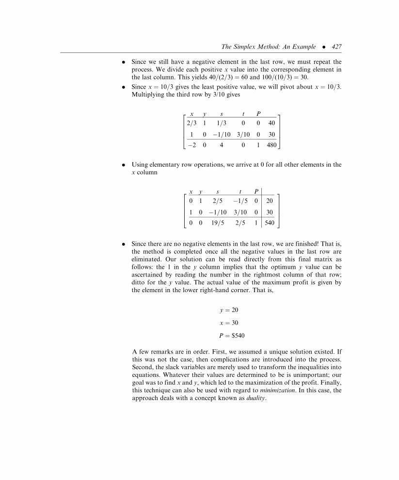
. Since we still have a negative element in the last row, we must repeat the
process. We divide each positive x value into the corresponding element in
the last column. This yields 40=(2=3) ¼ 60 and 100=(10=3) ¼ 30.
. Since x ¼ 10=3 gives the least positive value, we will pivot about x ¼ 10=3.
Multiplying the third row by 3/10 gives
x y s t P
2=3 1 1=3 0 0 40
1 0 �1=10 3=10 0 30
�2 0 4 0 1 480
26664
37775
. Using elementary row operations, we arrive at 0 for all other elements in the
x column
x y s t P
0 1 2=5 �1=5 0 20
1 0 �1=10 3=10 0 30
0 0 19=5 2=5 1 540
26664
37775
. Since there are no negative elements in the last row, we are finished! That is,
the method is completed once all the negative values in the last row are
eliminated. Our solution can be read directly from this final matrix as
follows: the 1 in the y column implies that the optimum y value can be
ascertained by reading the number in the rightmost column of that row;
ditto for the y value. The actual value of the maximum profit is given by
the element in the lower right-hand corner. That is,
y ¼ 20
x ¼ 30
P ¼ $540
A few remarks are in order. First, we assumed a unique solution existed. If
this was not the case, then complications are introduced into the process.
Second, the slack variables are merely used to transform the inequalities into
equations. Whatever their values are determined to be is unimportant; our
goal was to find x and y, which led to the maximization of the profit. Finally,
this technique can also be used with regard to minimization. In this case, the
approach deals with a concept known as duality.
The Simplex Method: An Example . 427

Problems Appendix D
(1) Solve the problem illustrated in this Appendix if the constraints are the same, but the
profit function is given by P(x, y) ¼ 7xþ 10y.
(2) Solve the problem illustrated in ithis Appendix if the constraints are the same, but
the profit function is given by P(x, y) ¼ 100xþ 10y.
(3) Solve the problem illustrated in this Appendix if both the ‘‘construction’’ and the
‘‘painting’’ constraints are both 600 hours and the profit function remains at
P(x, y) ¼ 10xþ 12y.
428 . Appendix D

Appendix E
A Word on NumericalTechniques and Technology
As we have demonstrated in this text, linear algebra is a very powerful tool. It
can be applied to such diverse areas as differential equations (see Chapter 4) and
to least-squares techniques (see Chapter 5). Yet the actual calculations needed to
arrive at solutions can be very tedious. The computation of higher-order deter-
minants (see Appendix A) and the application of the QR algorithm (see Section
5.3) can likewise require much time.
The field of numerical analysis can assist with calculations and, if appropriate,
with approximations. But even when numerical techniques are uses, one almost
always needs computational assistance in the form of technology.
One of the most useful tools is MATLAB1 (http://www.mathworks.com/prod-
ucts/matlab/).This software is employed by educators and is very useful with
respect to many topics in linear algebra.
Another software package is MATHEMATICA1 (http://www.wolfram.com/).
To illustrate this computer algebra system, the reader is asked to refer to the
modeling problem of Section 4.8.
The syntax for the system of differential equations is given by:
DSolve[{S1[t] ¼ 10� S1[t]=20, S20[t] ¼ S1[t]=50þ S3[t]=25� (6=50)�S2[t], S30[t]
¼ S3[t]=25þ S2[t]=50, S1[0] ¼ 0, S2[0] ¼ 0, S3[0] ¼ 0},
{S1[t], S2[t], S3[t]}, t]
The solution, obtained by hitting the ‘‘Shift’’ and ‘‘Enter’’ keys simultaneously, is
as follows:
429

[t]! 200 e�t=20 �1þ e
t=20� �
, S2[t]! 1
1491
50 e� t
20� 1
50(�2þ3
ffiffi2p
) t �1512 e150
(�2þ3ffiffi2p
) t � 330 et
20þ3ffiffi2p
t35þ 1
50(�2�3
ffiffi2p
) t
��� 205
ffiffiffi2p
et20þ3ffiffi2p
t25þ 1
50(�2�3
ffiffi2p
) t þ 1182 et
20þ 1
50(�2þ3
ffiffi2p
) t
þ 205ffiffiffi2p
et20þ 1
50(�2þ3
ffiffi2p
) t þ 330 et20þ 1
50(�2�3
ffiffi2p
) tþ 150
(�2þ3ffiffi2p
) t
þ 205ffiffiffi2p
et20þ 1
50(�2�3
ffiffi2p
) tþ 150
(�2þ3ffiffi2p
) t � 756 et10þ 1
50(�2�3
ffiffi2p
) tþ 150
(�2þ3ffiffi2p
) t
� 560ffiffiffi2p
et
10þ 1
50(�2�3
ffiffi2p
) tþ 150
(�2þ3ffiffi2p
) t þ 330 et
20þ 1
25(�2þ3
ffiffi2p
) t
� 205ffiffiffi2p
et20þ 1
25(�2þ3
ffiffi2p
) t � 756 et10þ 1
25(�2þ3
ffiffi2p
) t þ 560ffiffiffi2p
et10þ 1
25(�2þ3
ffiffi2p
) t
þ 756 et20þ 1
50(�2�3
ffiffi2p
) tþ 1100
(1þ6ffiffi2p
) t þ 560ffiffiffi2p
et20þ 1
50(�2�3
ffiffi2p
) tþ 1100
(1þ6ffiffi2p
) t
þ 756 et20þ 1
50(�2þ3
ffiffi2p
) tþ 1100
(1þ6ffiffi2p
) t � 560ffiffiffi2p
et20þ 1
50(�2þ3
ffiffi2p
) tþ 1100
(1þ6ffiffi2p
) t��
,
S3[t]! � 1
149150 e
� t20� 1
50(�2þ3
ffiffi2p
) t �336 e150
(�2þ3ffiffi2p
) t��
þ 45 et20þ3ffiffi2p
t25þ 1
50(�2�3
ffiffi2p
) t � 85ffiffiffi2p
et20þ3ffiffi2p
t25þ 1
50(�2�3
ffiffi2p
) t þ 381 et
20þ 1
50(�2þ3
ffiffi2p
) t
þ 85ffiffiffi2p
et
20þ 1
50(�2þ3
ffiffi2p
) t � 45 et20þ 1
50(�2�3
ffiffi2p
) tþ 150
(�2þ3ffiffi2p
) t
þ 85ffiffiffi2p
et
20þ 1
50(�2�3
ffiffi2p
) tþ 150
(�2þ3ffiffi2p
) t � 168 et10þ 1
50(�2�3
ffiffi2p
) tþ 150
(�2þ3ffiffi2p
) t
� 14ffiffiffi2p
et
10þ 1
50(�2�3
ffiffi2p
) tþ 150
(�2þ3ffiffi2p
) t � 45 et20þ 1
25(�2þ3
ffiffi2p
) t
� 85ffiffiffi2p
et
20þ 1
25(�2þ3
ffiffi2p
) t � 168 et10þ 1
25(�2þ3
ffiffi2p
) t þ 14ffiffiffi2p
et10þ 1
25(�2þ3
ffiffi2p
) t
þ 168 et20þ 1
50(�2�3
ffiffi2p
) tþ 1100
(1þ6ffiffi2p
) t þ 14ffiffiffi2p
et20þ 1
50(�2�3
ffiffi2p
) tþ 1100
(1þ6ffiffi2p
) t
þ 168 et20þ 1
50(�2þ3
ffiffi2p
) tþ 1100
(1þ6ffiffi2p
) t � 14ffiffiffi2p
et20þ 1
50(�2þ3
ffiffi2p
) tþ 1100
(1þ6ffiffi2p
) t��
One readily sees why this problem would be difficult to solve without technology.
430 . Appendix E

Answers and Hints to Selected Problems
Chapter 1
Section 1.1
(1) A is 2� 2, B is 2� 2, C is 2� 2, D is 4� 2, E is 4� 2,
F is 4� 2, G is 2� 3, H is 3� 3, J is 1� 5.
(2) a12 ¼ 2, a31 does not exist;
b12 ¼ 6, b31 does not exist;
c12 ¼ 0, c31 does not exist;
d12 ¼ 1, d31 ¼ 3;
e12 ¼ 2, e31 ¼ 5;
f12 ¼ 1, f31 ¼ 0;
g12 ¼ 1=3, e31 does not exist;
h12 ¼ffiffiffi3p
, h31 ¼ffiffiffi5p
;
j12 ¼ 0, j31 does not exist.
(3) a11 ¼ 1, a21 ¼ 3, b32 does not exist, d32 ¼ �2,
d23 does not exist, e22 ¼ �2, g23 ¼ �5=6,
h33 ¼ffiffiffi3p
, j21 does not exist.
(4) A, B, C, and H. (5) J is a row matrix.
(6)
1
2
3
4
26643775. (7) 1 4 9 16 25½ ].
(8) A ¼ 1 �1
�1 1
� �. (9) A ¼
1 1=2 1=32 1 2=33 3=2 1
24
35.
(10) B ¼1 0 �1
0 �1 �2
�1 �2 �3
24
35. (11) C ¼ 1 1 1 1
1 2 3 4
� �.
(12) D ¼0 �1 �2 �3
3 0 �1 �2
4 5 0 �1
24
35. (13)
2 4
6 8
� �.
431

(14)�5 �10
�15 �20
� �. (15)
9 3
�3 6
9 �6
6 18
2664
3775. (16)
�20 20
0 �20
50 �30
50 10
2664
3775.
(17)
0 �1
1 0
0 0
�2 �2
2664
3775. (18)
6 8
10 12
� �. (19)
0 2
6 1
� �.
(20)
1 3
�1 0
8 �5
7 7
2664
3775. (21)
3 2
�2 2
3 �2
4 8
2664
3775. (22) Does not exist.
(23)�4 �4
�4 �4
� �. (24)
�2 �2
0 �7
� �. (25)
5 �1
�1 4
�2 1
�3 5
2664
3775.
(26)
3 0
0 2
3 �2
0 4
2664
3775. (27)
17 22
27 32
� �. (28)
5 6
3 18
� �.
(29)�0:1 0:2
0:9 �0:2
� �. (30)
4 �3
�1 4
�10 6
�8 0
2664
3775. (31) X ¼ 4 4
4 4
� �.
(32) Y ¼ �11 �12
�11 �19
� �. (33) X ¼
11 1
�3 8
4 �3
1 17
2664
3775.
(34) Y ¼
�1:0 0:50:5 �1:02:5 �1:51:5 �0:5
2664
3775. (35) R ¼ �2:8 �1:6
3:6 �9:2
� �.
(36) S ¼
�1:5 1:0�1:0 �1:0�1:5 1:0
2:0 0
2664
3775.
(37)�u3 þ 6u2 þ u 6u� 6
21 �u3 � 2u2 � uþ 6=u
� �.
(38) [aij ]þ [bij ] ¼ [aij þ bij ] ¼ [bij þ aij ] ¼ [bij ]þ [aij ].
(39) [aij ]þ [0ij ] ¼ [aij þ 0ij ] ¼ [aij þ 0] ¼ [aij ].
(40) (l1 þ l2)[aij ] ¼ [(l1 þ l2)aij ] ¼ [l1aij þ l2aij ] ¼ [l1aij ]þ [l2aij ] ¼ l1[aij ]þ l2[aij ].
(41) (l1l2)[aij ] ¼ [(l1l2)aij ] ¼ [l1(l2aij)] ¼ l1[l2aij ] ¼ l1(l2[aij ]).
432 . Answers and Hints to Selected Problems

(42)
Refrigerators Stoves Washing machines Dryers
3 5 3 4 store 1
0 2 9 5 store 2
4 2 0 0 store 3
24
35
(43)
72 12 16
45 32 16
81 10 35
24
35.
(44)
Purchase price Interest rate
1,000 0:07
2,000 0:075
3,000 0:0725
264
375 first certificate
second certificate
third certificate
(45) (a) 200 150½ �, (b) 600 450½ �, (c) 550 350½ �.
(46) (b) 11 2 6 3½ �, (c) 9 4 10 8½ �.
(47) (b) 10,500 6,000 4,500½ �, (c) 35,500 14,500 3,300½ �.
Section 1.2
(1) (a) 2� 2, (b) 4� 4, (c) 2� 1, (d) Not defined, (e) 4� 2,
(f) 2� 4, (g) 4� 2, (h) Not defined, (i) Not defined, (j) 1� 4,
(k) 4� 4, (l) 4� 2.
(2)19 22
43 50
� �. (3)
23 34
31 46
� �. (4)
5 �4 3
9 �8 7
� �.
(5) A ¼ 13 �12 11
17 �16 15
� �. (6) Not defined. (7) �5 �6½ �.
(8) �9 �10½ �. (9) �7 4 �1½ �. (10) Not defined.
(11)1 �3
7 �3
� �. (12)
2 �2 2
7 �4 1
�8 4 0
24
35. (13) 1 3½ �.
(14) Not defined. (15) Not defined. (16) Not defined.
(17)
�1 �2 �1
1 0 �3
1 3 5
24
35. (18)
2 �2 1
2 0 0
1 �2 2
24
35. (19) �1 1 5½ �.
(21) AB ¼ 0. (22) AB ¼ AC ¼ 8 6
4 3
� �. (23) AB ¼ CB ¼ 8 16
2 4
� �.
(24)xþ 2y
3xþ 4y
� �. (25)
x� z
3xþ yþ z
xþ 3y
24
35. (26)
a11xþ a12y
a21xþ a22y
� �.
(27)b11xþ b12yþ b13z
b21xþ b22yþ b23z
� �. (28)
0 0
0 0
� �.
Chapter 1 . 433

(29)0 40
�16 8
� �. (30)
0 0 0
0 0 0
0 0 0
24
35.
(33) Let the ith row of an m� n matrix A be 0. If C ¼ AB, then for j ¼ 1, 2, . . . , n,
cij ¼Xn
k¼1
aikbkj ¼Xn
k¼1
(0)bkj ¼ 0
(34)1 2
3 4
� �1 1
0 0
� �¼ 1 1
3 3
� �.
(35) Let the jth column of an m� n matrix B be 0. If C ¼ AB, then for i ¼ 1, 2, . . . ,m,
cij ¼Xn
k¼1
aikbkj ¼Xn
k¼1
aik(0) ¼ 0
(36)1 0
1 0
� �1 2
3 4
� �¼ 1 2
1 2
� �.
(37) [aij ]([bij ][cij ]) ¼ [aij ]Xn
k¼1
bikckj
" #¼
Xmp¼1
aip
Xn
k¼1
bpkckj
!" #
¼Xmp¼1
Xn
k¼1
aipbpkckj
" #¼
Xn
k¼1
Xmp¼1
aipbpkckj
" #
¼Xn
k¼1
Xmp¼1
aipbpk
!ckj
" #
¼Xmp¼1
aipbpj
" #[cij ] ¼ ([aij ][bij ])[cij ]
(39)2 3
4 �5
� �x
y
� �¼ 10
11
� �. (40)
5 20
�1 4
� �x
y
� �¼ 80
�64
� �.
(41)
3 3
6 �8
�1 2
24
35 x
y
� �¼
100
300
500
24
35. (42)
1 3
2 �1
�2 �6
4 �9
�6 3
266664
377775 x
y
� �¼
4
1
�8
�5
�3
266664
377775.
(43)1 1 �1
3 2 4
� � x
y
z
2435 ¼ 0
0
� �. (44)
2 �1 0
0 �4 �1
� � x
y
z
2435 ¼ 12
15
� �.
(45)
1 2 �2
2 1 1
�1 1 �1
24
35 x
y
z
2435 ¼ �1 5 �2½ �. (46)
2 1 �1
1 2 1
3 �1 2
24
35 x
y
z
2435 ¼ 0
0
0
2435.
434 . Answers and Hints to Selected Problems

(47)
1 1 1
2 1 3
1 3 0
24
35 x
y
z
2435 ¼ 2
4
1
2435. (48)
1 2 �1
2 �1 2
2 2 �1
1 2 1
2664
3775 x
y
z
2435 ¼
5
1
7
3
26643775.
(49)
5 3 2 4
1 1 0 1
3 2 2 0
1 1 2 3
2664
3775
x
y
z
w
2664
3775 ¼
5
0
�3
4
2664
3775. (50)
2 �1 1 �1
1 2 �1 2
1 �3 2 �3
24
35 x
y
z
w
2664
3775 ¼ 1
�1
2
24
35.
(51) (a) pn ¼ [38,000], which is the total revenue for the flight.
(b) np ¼26,000 45,500 65,000
4,000 7,000 10,000
2,000 3,500 5,000
24
35, which is of no significance.
(52) (a) hP ¼ [ 9,625 9,762:50 9,887:50 10,100 9,887:50 ], which tabulates the
value of the portfolio each day.
(b) Ph does not exist.
(53) Tw ¼ [ 14:00 65:625 66:50 ]T, which tabulates the cost of producing each prod-
uct.
(54) qTw ¼ [33,862:50], which is the cost of producing all items on order.
(55) FC ¼613 625
887 960
1870 1915
24
35, which tabulates the number of each gender in each state of
sickness.
Section 1.3
(1) (a) (AB)T ¼ BTAT ¼�3 �1
6 �7
3 4
24
35, ATBT is not defined.
(b) (AB)T ¼ BTAT ¼ 18 40
24 52
� �, ATBT ¼
8 18 28
10 22 34
12 26 40
24
35.
(c) (AB)T ¼ BTAT ¼27 11 22
8 �19 56
�4 11 �23
24
35, ATBT ¼
8 2 �15
54 3 2
�27 6 �36
24
35.
(2)
7 4 �1
6 1 0
2 2 �6
24
35.
(3) xTx ¼ [29] and xxT ¼4 6 8
6 9 12
8 12 16
24
35.
(4) (a) BAT, (b) 2AT, (c) (BT þ C)A, (d) ABþ CT,
(e) ATAT þ ATA� AAT � AA.
(5) (a), (b), and (d).
Chapter 1 . 435
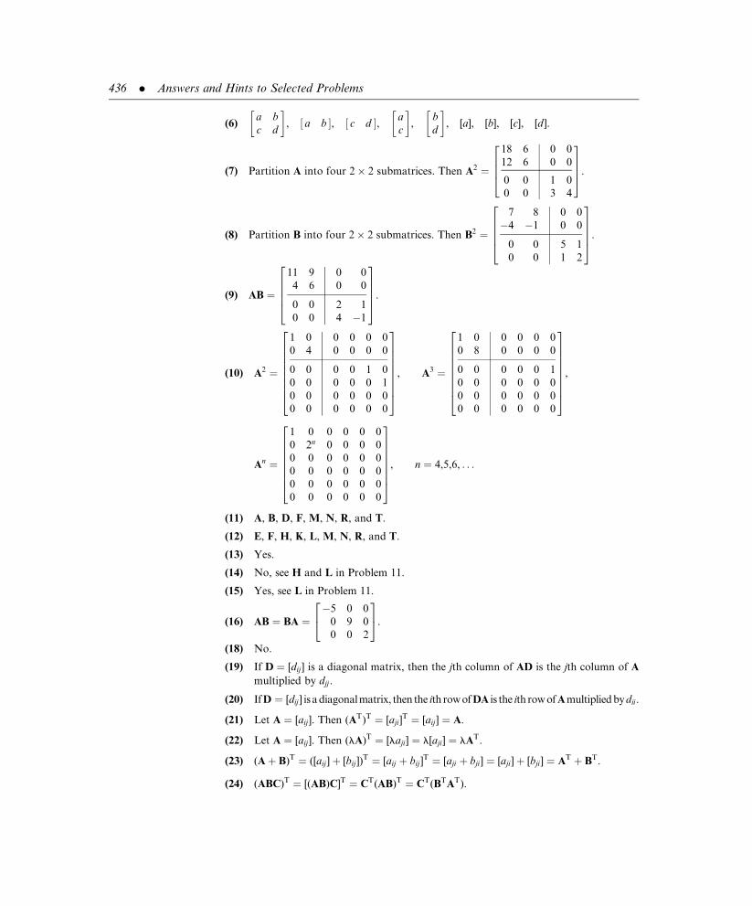
(6)a b
c d
� �, a b½ �, c d½ �, a
c
� �,
b
d
� �, [a], [b], [c], [d].
(7) Partition A into four 2� 2 submatrices. Then A2 ¼
18 6 0 0
12 6 0 0
0 0 1 0
0 0 3 4
2664
3775.
(8) Partition B into four 2� 2 submatrices. Then B2 ¼
7 8 0 0
�4 �1 0 0
0 0 5 1
0 0 1 2
26664
37775.
(9) AB ¼
11 9 0 0
4 6 0 0
0 0 2 1
0 0 4 �1
26664
37775.
(10) A2 ¼
1 0 0 0 0 0
0 4 0 0 0 0
0 0 0 0 1 0
0 0 0 0 0 1
0 0 0 0 0 0
0 0 0 0 0 0
266666664
377777775
, A3 ¼
1 0 0 0 0 0
0 8 0 0 0 0
0 0 0 0 0 1
0 0 0 0 0 0
0 0 0 0 0 0
0 0 0 0 0 0
266666664
377777775
,
An ¼
1 0 0 0 0 0
0 2n 0 0 0 0
0 0 0 0 0 0
0 0 0 0 0 0
0 0 0 0 0 0
0 0 0 0 0 0
26666664
37777775, n ¼ 4,5,6, . . .
(11) A, B, D, F, M, N, R, and T.
(12) E, F, H, K, L, M, N, R, and T.
(13) Yes.
(14) No, see H and L in Problem 11.
(15) Yes, see L in Problem 11.
(16) AB ¼ BA ¼�5 0 0
0 9 0
0 0 2
24
35.
(18) No.
(19) If D ¼ [dij ] is a diagonal matrix, then the jth column of AD is the jth column of A
multiplied by djj .
(20) IfD ¼ [dij ] is adiagonalmatrix, then the ith rowofDA is the ith rowofAmultipliedbydii.
(21) Let A ¼ [aij ]. Then (AT)T ¼ [aji]T ¼ [aij ] ¼ A.
(22) Let A ¼ [aij ]. Then (lA)T ¼ [laji] ¼ l[aji] ¼ lAT.
(23) (Aþ B)T ¼ ([aij ]þ [bij ])T ¼ [aij þ bij ]
T ¼ [aji þ bji] ¼ [aji]þ [bji] ¼ AT þ BT.
(24) (ABC)T ¼ [(AB)C]T ¼ CT(AB)T ¼ CT(BTAT).
436 . Answers and Hints to Selected Problems

(25) BT ¼ [(Aþ AT)=2]T ¼ 12(Aþ AT)T ¼ 1
2[AT þ (AT)T] ¼ 1
2(AT þ A) ¼ B.
(26) CT ¼ [(A� AT)=2]T ¼ 12(A� AT)T ¼ 1
2[AT � (AT)T]
¼ 12(AT � A) ¼ � 1
2(A� AT) ¼ �C.
(27) A ¼ 12(Aþ AT)þ 1
2(A� AT).
(28)
1 7=2 �1=27=2 1 5
�1=2 5 �8
24
35þ 0 3=2 �1=2
�3=2 0 �2
1=2 2 0
24
35.
(29)
6 3=2 1
3=2 0 �4
1 �4 2
24
35þ 0 �1=2 2
1=2 0 3
�2 �3 0
24
35.
(30) (AAT)T ¼ (AT)TAT ¼ AAT.
(31) Each diagonal element must equal its own negative and, therefore, must be zero.
(33) For any n� n matrix A, consider sequentially the equations ADi ¼ DiA, where all
the elements in Di (i ¼ 1,2, . . . ,n) are zero except for a single 1 in the i-i position.
Section 1.4
(1) (a) No. (b) Yes.
(2) (a) Yes. (b) No. (c) No.
(3) k ¼ 1.
(4) k ¼ 1=12.
(5) k is arbitrary; any value will work.
(6) xþ 2y ¼ 5
y ¼ 8
Solution: x ¼ �11, y ¼ 8
(7) x� 2yþ 3z ¼ 10
y� 5z ¼ �3
z ¼ 4
Solution: x ¼ 32, y ¼ 17, z ¼ 4
(8) x1 � 3x2 þ 12x3 ¼ 40
x2 � 5x3 ¼ �200
x3 ¼ 25
Solution: x1 ¼ �410,
x2 ¼ �50,
x3 ¼ 25
(9) xþ 3y ¼ �8
yþ 4z ¼ 2
0 ¼ 0
Solution: x ¼ �14þ 12z,
y ¼ z� 4z
(10) x1 � 7x2 þ 2x3 ¼ 0
x2 � x3 ¼ 0
0 ¼ 0
Solution: x1 ¼ 5x3,
x2 ¼ x3,
x3 is arbitrary
(11) x1 � x2 ¼ 1
x2 � 2x3 ¼ 2
x3 ¼ �3
0 ¼ 1
No solution
(12) x ¼ 51, y ¼ 23. (13) x ¼ �103, y ¼ 18.
(14) x ¼ 18:5, y ¼ �6. (15) x ¼ y ¼ 0.
Chapter 1 . 437
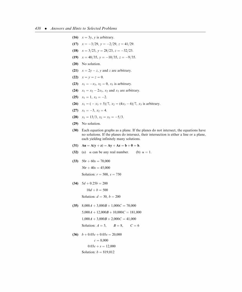
(16) x ¼ 3y, y is arbitrary.
(17) x ¼ �3=29, y ¼ �2=29, z ¼ 41=29.
(18) x ¼ 3=23, y ¼ 28=23, z ¼ �32=23.
(19) x ¼ 48=35, y ¼ �10=35, z ¼ �9=35.
(20) No solution.
(21) x ¼ 2y� z, y and z are arbitrary.
(22) x ¼ y ¼ z ¼ 0.
(23) x1 ¼ �x3, x2 ¼ 0, x3 is arbitrary.
(24) x1 ¼ x2 � 2x3, x2 and x3 are arbitrary.
(25) x1 ¼ 1, x2 ¼ �2.
(26) x1 ¼ (� x3 þ 5)=7, x2 ¼ (4x3 � 6)=7, x3 is arbitrary.
(27) x1 ¼ �3, x2 ¼ 4.
(28) x1 ¼ 13=3, x2 ¼ x3 ¼ �5=3.
(29) No solution.
(30) Each equation graphs as a plane. If the planes do not intersect, the equations have
no solutions. If the planes do intersect, their intersection is either a line or a plane,
each yielding infinitely many solutions.
(31) Au ¼ A(yþ z) ¼ Ayþ Az ¼ bþ 0 ¼ b.
(32) (a) a can be any real number. (b) a ¼ 1.
(33) 50rþ 60s ¼ 70,000
30rþ 40s ¼ 45,000
Solution: r ¼ 500, s ¼ 750
(34) 5d þ 0:25b ¼ 200
10d þ b ¼ 500
Solution: d ¼ 30, b ¼ 200
(35) 8,000Aþ 3,000Bþ 1,000C ¼ 70,000
5,000Aþ 12,000Bþ 10,000C ¼ 181,000
1,000Aþ 3,000Bþ 2,000C ¼ 41,000
Solution: A ¼ 5, B ¼ 8, C ¼ 6
(36) bþ 0:05cþ 0:05s ¼ 20,000
c ¼ 8,000
0:03cþ s ¼ 12,000
Solution: b ¼ $19,012
438 . Answers and Hints to Selected Problems
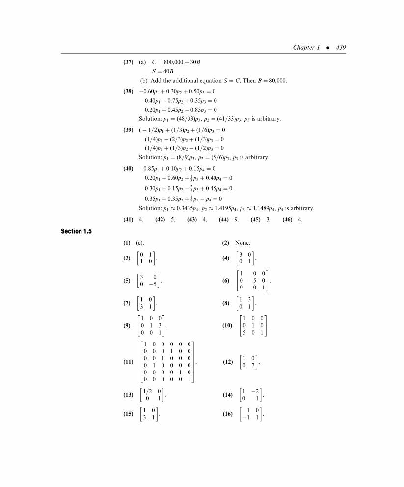
(37) (a) C ¼ 800,000þ 30B
S ¼ 40B
(b) Add the additional equation S ¼ C. Then B ¼ 80,000.
(38) �0:60p1 þ 0:30p2 þ 0:50p3 ¼ 0
0:40p1 � 0:75p2 þ 0:35p3 ¼ 0
0:20p1 þ 0:45p2 � 0:85p3 ¼ 0
Solution: p1 ¼ (48=33)p3, p2 ¼ (41=33)p3, p3 is arbitrary.
(39) (� 1=2)p1 þ (1=3)p2 þ (1=6)p3 ¼ 0
(1=4)p1 � (2=3)p2 þ (1=3)p3 ¼ 0
(1=4)p1 þ (1=3)p2 � (1=2)p3 ¼ 0
Solution: p1 ¼ (8=9)p3, p2 ¼ (5=6)p3, p3 is arbitrary.
(40) �0:85p1 þ 0:10p2 þ 0:15p4 ¼ 0
0:20p1 � 0:60p2 þ 13p3 þ 0:40p4 ¼ 0
0:30p1 þ 0:15p2 � 23p3 þ 0:45p4 ¼ 0
0:35p1 þ 0:35p2 þ 13p3 � p4 ¼ 0
Solution: p1 � 0:3435p4, p2 � 1:4195p4, p3 � 1:1489p4, p4 is arbitrary.
(41) 4. (42) 5. (43) 4. (44) 9. (45) 3. (46) 4.
Section 1.5
(1) (c). (2) None.
(3)0 1
1 0
� �. (4)
3 0
0 1
� �.
(5)3 0
0 �5
� �. (6)
1 0 0
0 �5 0
0 0 1
24
35.
(7)1 0
3 1
� �. (8)
1 3
0 1
� �.
(9)
1 0 0
0 1 3
0 0 1
24
35. (10)
1 0 0
0 1 0
5 0 1
24
35.
(11)
1 0 0 0 0 0
0 0 0 1 0 0
0 0 1 0 0 0
0 1 0 0 0 0
0 0 0 0 1 0
0 0 0 0 0 1
26666664
37777775. (12)
1 0
0 7
� �.
(13)1=2 0
0 1
� �. (14)
1 �2
0 1
� �.
(15)1 0
3 1
� �. (16)
1 0
�1 1
� �.
Chapter 1 . 439

(17)
1 0 0
0 1=2 0
0 0 1
24
35. (18)
0 1 0
1 0 0
0 0 1
24
35. (19)
1 0 �3
0 1 0
0 0 1
24
35.
(20)
1 0 0
0 1 2
0 0 1
24
35. (21)
1 0 0 0
0 1 0 0
0 0 0 1
0 0 1 0
2664
3775. (22)
1 0 0 0
0 1 0 0
3 0 1 0
0 0 0 1
2664
3775.
(23)4 �1
�3 1
� �. (24)
1
3
2 �1
�1 2
� �. (25) Does not exist.
(26)1
2
1 1 �1
1 �1 1
�1 1 1
24
35. (27)
0 1 0
0 0 1
1 0 0
24
35.
(28)
�1 �1 1
6 5 �4
�3 �2 2
24
35. (29) Does not exist.
(30)1
2
1 0 0
�5 2 0
1 �2 2
24
35. (31)
1
6
3 �1 �8
0 2 1
0 0 3
24
35.
(32)
9 �5 �2
5 �3 �1
�36 21 8
24
35. (33)
1
17
1 7 �2
7 �2 3
�2 3 4
24
35.
(34)1
17
14 5 �6
�5 �3 7
13 1 �8
24
35. (35) Does not exist.
(36)1
33
5 3 1
�6 3 12
�8 15 5
24
35. (37)
1
4
0 �4 4
1 5 �4
3 7 �8
24
35.
(38)1
4
4 �4 �4 �4
0 4 2 5
0 0 2 3
0 0 0 �2
2664
3775. (39)
1 0 0 0
2 �1 0 0
�8 3 1=2 0
�25 10 2 �1
2664
3775.
(41) (a)4 �1
�3 1
� �. (b)
4 �6
�6 12
� �.
(42) x ¼ 1, y ¼ �2.
(43) a ¼ �3, b ¼ 4.
(44) x ¼ 2, y ¼ �1.
(45) l ¼ 1, p ¼ 3.
(46) Not possible; the coefficient matrix is singular.
(47) x ¼ �8, y ¼ 5, z ¼ 3.
440 . Answers and Hints to Selected Problems

(48) x ¼ y ¼ z ¼ 1.
(49) l ¼ 1, m ¼ �2, n ¼ 0.
(50) Not possible; the coefficient matrix is singular.
(51) x ¼ y ¼ z ¼ 1.
(52) (a) x ¼ 70, y ¼ �40.
(b) x ¼ 134, y ¼ �82.
(c) x ¼ 1:9, y ¼ �1:1.
(d) x ¼ 25, y ¼ �15.
(53) (a) x ¼ 13=3, y ¼ �5=3, z ¼ �5=3.
(b) x ¼ 113=30, y ¼ �34=30, z ¼ �31=30.
(c) x ¼ 79=15, y ¼ �32=15, z ¼ �38=15.
(d) x ¼ 41=10, y ¼ �18=10, z ¼ �17=10.
(54) (a) A�2 ¼ 11 �4
�8 3
� �, A�3 ¼ 41 �15
�30 11
� �.
(b) A�2 ¼ 9 �20
�4 9
� �, A�3 ¼ �38 85
17 �38
� �.
(c) A�2 ¼ 19 �5
�15 4
� �, A�3 ¼ 91 �24
�72 19
� �.
(d) A�2 ¼1 �2 1
0 1 �2
0 0 1
24
35, A�3 ¼
1 �3 3
0 1 �3
0 0 1
24
35.
(e) A�2 ¼1 �4 �4
0 1 2
0 0 1
24
35, A�3 ¼
1 �6 �9
0 1 3
0 0 1
24
35.
(56) Use the result of Problem 19 or Problem 20 of Section 1.3.
(58) (BA�1)T(A�1BT)�1 ¼ [(A�1)TBT][(BT)�1(A�1)�1] ¼ [(AT)�1BT)][(BT)�1A]
¼ A�1[BT(BT)�1]A ¼ A�1IA ¼ A�1A ¼ I.
(60) [(1=l)A�1][lA] ¼ (1=l)(l)A�1A ¼ 1I ¼ I.
(61) (ABC)�1 ¼ [(AB)C]�1 ¼ C�1(AB)�1 ¼ C�1(B�1A�1).
Section 1.6
(1)1 0
3 1
� �1 1
0 1
� �, x ¼ 10
�9
� �.
(2)1 0
0:5 1
� �2 1
0 1:5
� �, x ¼ 8
�5
� �.
(3)1 0
0:625 1
� �8 3
0 0:125
� �, x ¼ �400
1275
� �.
Chapter 1 . 441

(4)
1 0 0
1 1 0
0 �1 1
24
35 1 1 0
0 �1 1
0 0 2
24
35, x ¼
3
1
�2
24
35.
(5)
1 0 0
�1 1 0
�2 �2 1
24
35 �1 2 0
0 �1 1
0 0 5
24
35, x ¼
5
2
�1
24
35.
(6)
1 0 0
2 1 0
�1 0 1
24
35 2 1 3
0 �1 �6
0 0 1
24
35, x ¼
�10
0
10
24
35.
(7)
1 0 043
1 0
1 � 218
1
264
375
3 2 1
0 � 83� 1
3
0 0 18
264
375, x ¼
10
�10
40
24
35.
(8)
1 0 0
2 1 0
�1 �0:75 1
24
35 1 2 �1
0 �4 3
0 0 4:25
24
35, x ¼
79
1
1
24
35.
(9)
1 0 0
0 1 0
0 0 1
24
35 1 2 �1
0 2 1
0 0 1
24
35, x ¼
19
�3
5
24
35.
(10)
1 0 0
3 1 0
1 12
1
264
375
1 0 0
0 2 0
0 0 2
264
375, x ¼
2
�1
1=2
24
35.
(11)
1 0 0 0
1 1 0 0
1 1 1 0
0 1 2 1
266664
377775
1 0 1 1
0 1 �1 0
0 0 1 �1
0 0 0 3
266664
377775, x ¼
1
�5
2
1
2664
3775.
(12)
1 0 0 0
12
1 0 0
0 0 1 0
0 27
57
1
266664
377775
2 1 �1 3
0 72
52� 1
2
0 0 �1 1
0 0 0 37
266664
377775, x �
266:67
�166:67
166:67
266:67
2664
3775.
(13)
1 0 0 0
1 1 0 0
1 1 1 0
0 �1 �2 1
266664
377775
1 2 1 1
0 �1 1 0
0 0 �1 1
0 0 0 3
266664
377775, x ¼
10
10
10
�10
2664
3775.
(14)
1 0 0 0
1 1 0 0
�2 1:5 1 0
0:5 0 0:25 1
266664
377775
2 0 2 0
0 2 �2 6
0 0 8 �8
0 0 0 3
266664
377775, x ¼
�2:5�1:5
1:52:0
2664
3775.
(15) (a) x ¼ 5, y ¼ �2; (b) x ¼ �5=7, y ¼ 1=7.
442 . Answers and Hints to Selected Problems

(16) (a) x ¼ 1, y ¼ 0, z ¼ 2; (b) x ¼ 140, y ¼ �50, z ¼ �20.
(17) (a)
8
�3
�1
24
35, (b)
2
0
0
2435, (c)
35
5
15
24
35, (d)
�0:51:51:5
24
35.
(18) (a)
�1
�1
1
1
2664
3775, (b)
0
0
0
0
26643775, (c)
80
50
�10
20
2664
3775, (d)
�1=31=31=31=3
2664
3775.
(21) (d) A is singular.
Section 1.7
(1)
1 43 52−1−4 −3−5 −2
5
4
3
2
1
−1
−2
−3
−4
−5
y
xu
u+vv
(4)
1 43 52−1−4 −3−5 −2
54
3
21
−1
−2−3−4
y
x
y
x
x+y
6
Chapter 1 . 443

(6)
1 432−1−3 −2
5
4
3
2
1
−1
−2
−3
−4
y
xy
x
y−x
(7)
1 43 52−1−4 −3 −2
5
4
3
2
1
−1
−2
−3
y
xu
v u−v
6
444 . Answers and Hints to Selected Problems

(10)
12
1098765432
−2−2−4−6−8−10
−4
−6
−8
−10
1
1
z
y
x
2z
2 3 4 5 6 7 8 910 12
(12)
12
1098765432
−2−2−4−6−8−10−12
−4
−6
−8
−10
1
1
z
y
x
−2z
2 3 4 5 6 7 8 910 12
Chapter 1 . 445

(17) (a) 341.578, (b) 111.808, (c) 2258,(d) 59.048, (e) 2708.
(19)ffiffiffi2p
. (20) 5. (21)ffiffiffi5p
. (22)ffiffiffi3p
.
(23)ffiffiffiffiffiffiffiffi3=4
p. (24)
ffiffiffi3p
. (25)ffiffiffiffiffi15p
. (26) 2.
(27)ffiffiffi2p
. (28)ffiffiffiffiffi39p
. (29)ffiffiffi5p
.
(16)
1
1
w
w
x
y
14
2
3
−1
−1
−2
−3
−4
−2−3−4 4−5
2 3 4
w1−
(30)
4
3
2
1
(3,1,2)
(3,1,0)
(3,0,0)
11
2
3
4
5
2y
z
x
3 4
446 . Answers and Hints to Selected Problems

(33) z
5
5
4
4
3
3
2
2
1
1y
x
(−1, 2, 3)
(−1, 2, 3)(−1, 0, 0) −1
−2
−3
−4
−5
(38)
y
z
x
(1000, −500, 200)
(1000, −500, 0)(1000, 0, 0)
800
600
400
200
200400
600800
10001200
−100
0−8
00−6
00−4
00−2
00
(39)
z
x
y
(−400, −50, −300)
(−400, −50, 0)
−50
−450−400−350−300−250−200−150−50
−100
−100−150−200
−200
−150
−100
−50
−250
−300
−350
(−400, 0, 0)
Chapter 1 . 447

(40) Not normalized. (41) Not normalized. (42) Normalized.
(43) Normalized. (44) Not normalized. (45) Normalized.
(46) Normalized. (47) Normalized. (48) Normalized.
Chapter 2
Section 2.1(1) Vector space. (2) Violates (A1).
(3) Vector space. (4) Vector space.
(5) Violates (A1). (6) Violates (A1).
(7) Vector space. (8) Violates (S1) with negative scalars.
(9) Violates (A1). (10) Vector space.
(11) Violates (A4). (12) Violates (A1).
(13) Vector space. (14) Violates (S3).
(15) Violates (S3). (16) Violates (S3).
(17) Violates (S3). (18) Violates (A4).
(19) Violates (A5). (20) Violates (S4).
(21) Violates (S5). (22) Violates (S5).
(23) Violates (S3). (24) Vector space.
(25) Violates (A1). (26) Vector space.
(27) Violates (A4). (28) Vector space.
(29) Vector space. (30) Violates (A5) for f (t) � 0.
(31) Violates (A2). (32) Vector space.
(34) Let 01 and 02 be two zero vectors. Then 01 ¼ 01 þ 02 ¼ 02.
(35) v� (u� v) ¼ v� (u��v) ¼ v� (� v� u) ¼ (v��v)� u ¼ 0� u ¼ u.
(36) v ¼ 0� v ¼ (� u� u)� v ¼ �u� (u� v)
¼ �u� (u� w) ¼ (� u� u)� w ¼ 0� w ¼ 0.
(37) u� u ¼ 1� u� 1� u ¼ (1þ 1)� u ¼ 2� u.
(38) Given 2� u ¼ 2� v. Then,
u¼1�u¼(12�2)�u¼1
2�(2�u)¼1
2�(2�v)¼(1
2�2)�v¼1�v¼v.
448 . Answers and Hints to Selected Problems

(39) First show that �b� u ¼ (� b)� u. Then
0 ¼ (a� u)� (� b� u) ¼ a� u� (� b)� u ¼ [aþ (� b)]� u ¼ (a� b)� u
and the result follows from Theorem 7.
(40) 0� 0 ¼ 0. Thus, 0 is an additive inverse of 0, and the additive inverse is unique.
Section 2.2Problems 4, 5, 9, 11, 13, 16, 20, 21, 22, 24, and 25 are not subspaces; all the others are
subspaces.
(28) (a) and (c). (29) (a) and (c).
(30) (a) and (c). (31) (a) and (c).
(32) All except (f). (33) (b), (c), (d), and (e).
(34) (b), (c), (d), and (e). (35) (a), (b), and (c).
(36)x
y
� �2 R2
� ����y ¼ 2x
�. (37)
a b
c d
� �2M2�2
� ����d ¼ 0
�.
(38) a3t3 þ a2t
2 þ at þ a0e P3ja0 ¼ 0� �
.
(39) The straight line through the origin defined by the equation y ¼ �5x in an x� y
coordinate system.
(40) Such a straight line satisfies the equation y ¼ ax, for any fixed choice of the scalar
a. The set of points on this line isx
y
� �2 R2
� ����y ¼ ax
�.
(41) The line does not include the origin.
(43) Given that u ¼Pni¼1
civi and vi ¼Pmj¼1
aijwj . Then,
u ¼Pni¼1
ci
Pmj¼1
aijwj
!¼Pni¼1
Pmj¼1
ciaijwj ¼Pmj¼1
Pni¼1
ciaij
wj .
Define dj ¼Pni¼1
ciaij .
(44) Denote the columns of A as A1,A2, . . . ,An and x ¼ x1 x2 . . . xn½ ]T. Then
y ¼ x1A1 þ x2A2 þ . . .þ xnAn.
(45) Let Ay ¼ Az ¼ 0. Then A(ayþ bz) ¼ a(Ay)þ b(Az) ¼ a(0)þ b(0) ¼ 0.
(46) A(2x) ¼ 2(Ax) ¼ 2b 6¼ b.
Chapter 2 . 449
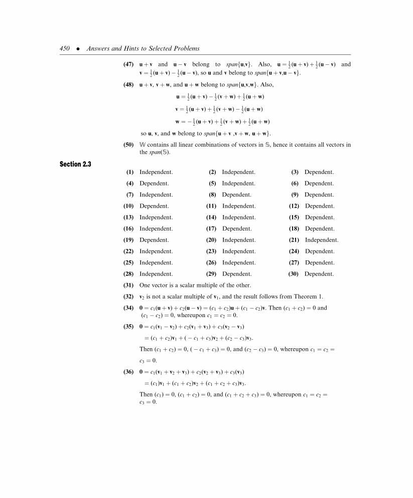
(47) uþ v and u� v belong to spanfu,vg. Also, u ¼ 12(uþ v)þ 1
2(u� v) and
v ¼ 12(uþ v)� 1
2(u� v), so u and v belong to spanfuþ v,u� vg.
(48) uþ v, vþ w, and uþ w belong to spanfu,v,wg. Also,
u ¼ 12(uþ v)� 1
2(vþ w)þ 1
2(uþ w)
v ¼ 12(uþ v)þ 1
2(vþ w)� 1
2(uþ w)
w ¼ � 12(uþ v)þ 1
2(vþ w)þ 1
2(uþ w)
so u, v, and w belong to spanfuþ v ,vþ w, uþ wg.
(50) W contains all linear combinations of vectors in S, hence it contains all vectors in
the span(S).
Section 2.3(1) Independent. (2) Independent. (3) Dependent.
(4) Dependent. (5) Independent. (6) Dependent.
(7) Independent. (8) Dependent. (9) Dependent.
(10) Dependent. (11) Independent. (12) Dependent.
(13) Independent. (14) Independent. (15) Dependent.
(16) Independent. (17) Dependent. (18) Dependent.
(19) Dependent. (20) Independent. (21) Independent.
(22) Independent. (23) Independent. (24) Dependent.
(25) Independent. (26) Independent. (27) Dependent.
(28) Independent. (29) Dependent. (30) Dependent.
(31) One vector is a scalar multiple of the other.
(32) v2 is not a scalar multiple of v1, and the result follows from Theorem 1.
(34) 0 ¼ c1(uþ v)þ c2(u� v) ¼ (c1 þ c2)uþ (c1 � c2)v. Then (c1 þ c2) ¼ 0 and
(c1 � c2) ¼ 0, whereupon c1 ¼ c2 ¼ 0.
(35) 0 ¼ c1(v1 � v2)þ c2(v1 þ v3)þ c3(v2 � v3)
¼ (c1 þ c2)v1 þ (� c1 þ c3)v2 þ (c2 � c3)v3.
Then (c1 þ c2) ¼ 0, (� c1 þ c3) ¼ 0, and (c2 � c3) ¼ 0, whereupon c1 ¼ c2 ¼
c3 ¼ 0.
(36) 0 ¼ c1(v1 þ v2 þ v3)þ c2(v2 þ v3)þ c3(v3)
¼ (c1)v1 þ (c1 þ c2)v2 þ (c1 þ c2 þ c3)v3.
Then (c1) ¼ 0, (c1 þ c2) ¼ 0, and (c1 þ c2 þ c3) ¼ 0, whereupon c1 ¼ c2 ¼c3 ¼ 0.
450 . Answers and Hints to Selected Problems
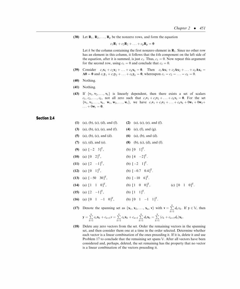
(38) Let R1, R2, . . . , Rp be the nonzero rows, and form the equation
c1R1 þ c2R2 þ . . .þ cpRp ¼ 0
Let k be the column containing the first nonzero element in R1. Since no other row
has an element in this column, it follows that the kth component on the left side of
the equation, after it is summed, is just c1. Thus, c1 ¼ 0. Now repeat this argument
for the second row, using c1 ¼ 0 and conclude that c2 ¼ 0.
(39) Consider c1x1 þ c2x2 þ . . .þ ckxk ¼ 0. Then c1Ax1 þ c2Ax2 þ . . .þ ckAxk ¼A0 ¼ 0 and c1y1 þ c2y2 þ . . .þ ckyk ¼ 0, whereupon c1 ¼ c2 ¼ . . . ¼ ck ¼ 0.
(40) Nothing.
(41) Nothing.
(43) If fv1, v2, . . . , vkg is linearly dependent, then there exists a set of scalars
c1, c2, . . . , ck, not all zero such that c1v1 þ c2v2 þ . . .þ ckvk ¼ 0. For the set
fv1, v2, . . . , vk, w1, w2, . . . , wrg, we have c1v1 þ c2v2 þ . . .þ ckvk þ 0w1 þ 0w2þ. . .þ 0wr ¼ 0.
Section 2.4(1) (a), (b), (c), (d), and (f). (2) (a), (c), (e), and (f).
(3) (a), (b), (c), (e), and (f). (4) (e), (f), and (g).
(5) (a), (b), (c), and (d). (6) (a), (b), and (d).
(7) (c), (d), and (e). (8) (b), (c), (d), and (f).
(9) (a) [�2 3 ]T, (b) [ 0 1 ]T.
(10) (a) [ 0 2 ]T, (b) [ 4 �2 ]T.
(11) (a) [ 2 �1 ]T, (b) [�2 1 ]T.
(12) (a) [ 0 1 ]T, (b) [�0:7 0:4 ]T.
(13) (a) [�50 30 ]T, (b) [�10 6 ]T.
(14) (a) [ 1 1 0 ]T, (b) [ 1 0 0 ]T, (c) [ 0 1 0 ]T.
(15) (a) [ 2 �1 ]T, (b) [ 1 1 ]T.
(16) (a) [ 0 1 �1 0 ]T, (b) [ 0 1 �1 1 ]T.
(17) Denote the spanning set as fx1, x2, . . . , xn, vg with v ¼Pnk¼1
dkxk. If y 2 V, then
y ¼Pnk¼1
ckxk þ cnþ1v ¼Pnk¼1
ckxk þ cnþ1
Pnk¼1
dkxk ¼Pnk¼1
ck þ cnþ1dkð Þxk.
(18) Delete any zero vectors from the set. Order the remaining vectors in the spanning
set, and then consider them one at a time in the order selected. Determine whether
each vector is a linear combination of the ones preceding it. If it is, delete it and use
Problem 17 to conclude that the remaining set spans V. After all vectors have been
considered and, perhaps, deleted, the set remaining has the property that no vector
is a linear combination of the vectors preceding it.
Chapter 2 . 451

(19) First four matrices.
(20) f[ 1 1 ], [ 1 2 ]g.
(21) ft2 þ t, tþ 1, t2 þ 1g.
(23) ft2 þ 2t� 3, t2 þ 5t, 2t2 � 4, t3g.
(24) f[ 1 2 1 ]T, [ 1 2 0 ]T, [ 1 0 0 ]Tg.
(25) ft3 þ t2 þ t, t2 þ tþ 1, tþ 1, t3g.
(26) If it did, then the process described in Problem 18 would yield a basis having less
vectors than the dimension of the vector space.
(27) If the second vector is not a scalar multiple of the first vector, then the second vector
is not a linear combination of the first, and the two vectors are linearly independent.
(28) Choose a basis for W, then use the results of Problem 22.
(29) Let fw1, w2, . . . , wmg be a basis for W and extend it into a basis for V.
(30) Use Problem 26.
(31) Use Problem 18.
Section 2.5(1) [ 1 1 2 ]T, [ 0 1 4=3 ]T. (2) [ 1 1 2 ]T, [ 0 1 4 ]T, [ 0 0 1 ]T.
(3) [ 1 12
1 ]T. (4) [ 1 0 2 ]T, [ 0 1 1 ]T.
(5) First two vectors. (6) [1 0 0 1 ], [ 0 1 1 1], [0 0 1 1].
(7) [ 1 0 �1 1 ], [ 0 1 3 �2 ],
[ 0 0 1 0 ].
(8) Standard basis for Rn.
(9) [1 2 4 0 ], [0 1 4=3 �1=3 ]. (10) t2þ 1, tþ 1, 1.
(11) t2 þ tþ 1, tþ 14. (12) t, 1.
(13) First two vectors. (14) First two vectors.
(15) t3 þ t2 � t, t2 þ tþ 1. (16) t3 þ 12t2 þ 1
2, t2 þ t, tþ 1.
(17) t3 þ 3t2, t2 þ 1, tþ 1. (18) First two vectors.
(19)1 1
1 0
� �,
0 1
1 0
� �,
0 0
1 0
� �. (20) First two vectors.
(21)1 3
1 2
� �,
0 1
0 1
� �.
(22) Independent. (23) Independent. (24) Dependent.
(25) Independent. (26) Dependent. (27) Dependent.
(28) Dependent. (29) Independent. (30) Independent.
452 . Answers and Hints to Selected Problems

(31) Dependent. (32) Independent. (33) Dependent.
(34) Dependent. (35) Independent. (36) Independent.
(37) Dependent. (38) Independent. (39) Independent.
(40) Dependent. (41) Independent. (42) Dependent.
(43) Dependent. (44) No
(45) k ¼ row rank � number of rows ¼ m. Also, each row, considered as a row matrix,
is an n-tuple and, therefore, an element in an n-dimensional vector space. Every
subset of such vectors contains most n-linearly independent vectors (Corollary 1 of
Section 2.4), thus k � n.
Section 2.6(1) 2. (2) 1. (3) 2. (4) 1. (5) 1.
(6) 2. (7) 3. (8) 2. (9) 3. (10) 4.
(11) Row rank � 3. (12) Column rank � 2. (13) 0.
(14) (a) No, (b) Yes.
(15) (a) Yes, (b) Yes, (c) No.
(16) (a) Yes, (b) No, (c) Yes.
(17) Consistent with no arbitrary unknowns: x ¼ 2=3, y ¼ 1=3.
(18) Inconsistent.
(19) Consistent with one arbitrary unknown: x ¼ (1=2)(3� 2z), y ¼ �1=2.
(20) Consistent with two arbitrary unknowns: x ¼ (1=7)(11� 5z� 2w),
y ¼ (1=7)(1� 3zþ 3w).
(21) Consistent with no arbitrary unknowns: x ¼ y ¼ 1, z ¼ �1.
(22) Consistent with no arbitrary unknowns: x ¼ y ¼ 0.
(23) Consistent with no arbitrary unknowns: x ¼ y ¼ z ¼ 0.
(24) Consistent with one arbitrary unknown: x ¼ �z, y ¼ z.
(25) Consistent with two arbitrary unknowns: x ¼ z� 7w, y ¼ 2z� 2w.
Chapter 3
Section 3.1(1) Function; image ¼ f1, 2, 3, 4, 5g. (2) Not a function.
(3) Not a function. (4) Function; image ¼ f2, 4g.
(5) Not a function. (6) Function; image ¼ f10, 30, 40, 50g.
(7) Not a function. (8) Function; image ¼ f6g.
Chapter 3 . 453

(9) Function; image ¼ fa, c, d, f g. (10) Function; image ¼ fa, b, c, d, f g.
(11) Not a function. (12) Function; image ¼ f2, 4, 6, 8, 10g.
(13) Not a function. (14) Function; image ¼ fblue, yellowg.
(15) Function; image ¼ f10:3, 18:6, 22:7g.
(16) Function. (17) Function. (18) Not a function.
(19) Function. (20) Not a function. (21) Not a function.
(22) Function. (23) Not a function. (24) Function.
(25) Function. (26) Not a function.
(27) A function when the domain is restricted to be all real numbers excluding
�3 < x < 3.
(28) Not a function.
(29) A function when the domain is limited to �4 � x � 4.
(30) (a) No, (b) Yes, (c) No, (d) Yes.
(31) (a) 2, (b) 0, (c) 6, (d) 4x2 � 6xþ 2.
(32) (a) 1, (b) 3, (c) 8x2 � 2x, (d) 2a2 þ 4abþ 2b2 � a� b.
(33) (a) �9, (b) �1, (c) 8z3 � 1,
(d) a3 � 3a2bþ 3ab2 � b3 � 1.
(34) Neither is onto.
(35) 1, 12, and 15.
(36) Figure 3.1 is one-to-one; Figure 3.2 is not.
(37) 1, 6, and 10.
Section 3.2(1) (a) 4 9½ ], (b) �2 15½ ], (c) �16 600½ ],
(d) 0 �21½ ].
(2) (a) 4 1½ ], (b) 1 3½ ], (c) �6 198½ ],
(d) 2 �9½ ].
(3) (a) 3 3½ ], (b) 1 �3½ ], (c) 0 0½ ],
(d) 5 3½ ].
(4) (a) �2 1½ ], (b) 1 �6½ ], (c) 2 2½ ],
(d) �2 �1½ ].
(5) (a) �4 0½ ], (b) �5 0½ ], (c) �2 0½ ],
(d) 0 0½ ].
454 . Answers and Hints to Selected Problems

(6) (a) 2 3 3½ ], (b) �1 1 �1½ ],
(c) 3 6 2½ ], (d) 0 0 2½ ].
(7) (a) 2 1 0½ ], (b) �1 �6 5½ ],
(c) 3 0 3½ ], (d) 0 0 0½ ].
(8) (a)3 1
4 2
� �, (b)
3 1
3 �1
� �,
(c)�5 10
0 20
� �, (d)
13 28
44 �32
� �.
(9) (a)3 0
0 �1
� �, (b)
0 0
0 0
� �,
(c)30 0
0 �5
� �, (d)
�4 0
0 �31
� �.
(10) (a) 5t2 � 7t, (b) �t2 þ 2t,
(c) �3t2 þ 3t, (d) �3t2 þ 3t.
(11) Linear. (12) Not linear. (13) Not linear.
(14) Not linear. (15) Linear. (16) Linear.
(17) Linear. (18) Not linear. (19) Linear.
(20) Linear. (21) Not linear. (22) Linear.
(23) Linear. (24) Linear. (25) Not linear.
(26) Linear. (27) Not linear. (28) Linear.
(29) Linear. (30) Linear. (31) Not linear.
(32) Not linear. (33) Linear. (34) Linear.
(35) Linear. (36) Linear. (37) Linear.
(38) Linear. (39) Linear. (40) Not linear.
(41) Linear. (42) Not linear.
(43) I(auþ bv) ¼ auþ bv ¼ aI(u)þ bI(v).
(44) If v 2 V, then v ¼Pni¼1
civi and
L(v) ¼ LPni¼1
civi
¼Pni¼1
ciL við Þ ¼Pni¼1
civi ¼ v.
(45) 0(auþ bv) ¼ 0 ¼ a0þ b0 ¼ a0(u)þ b0(v).
Chapter 3 . 455

(46) If v 2 V, then v ¼Pni¼1
civi and
L(v) ¼ LPni¼1
civi
¼Pni¼1
ciL við Þ ¼Pni¼1
ci0 ¼ 0:
(47) T(auþ bv) ¼ T(au)þ T(bv) from equation (3:2)
¼ aT(u)þ bT(v) from equation (3:3)
(48) Linear. (49) �2. (50) 3u� v. (51) 2v.
(52) L(v1 þ v2 þ v3) ¼ L[v1 þ (v2 þ v3)] ¼ L(v1)þ L(v2 þ v3)
¼ L(v1)þ L(v2)þ L(v3):
(53) (S þ T)(auþ bv) ¼ S(auþ bv)þ T(auþ bv)
¼ [aS(u)þ bS(v)]þ [aT(u)þ bT(v)]
¼ a[S(u)þ T(u)]þ b[S(v)þ T(v)]
¼ a(S þ T)(u)þ b(S þ T)(v):
(54) (kT) (auþ bv) ¼ k [T(auþ bv)] ¼ k [aT(u)þ bT(v)]
¼ a[kT(u)]þ b[kT(v)]
¼ a(kT)(u)þ b(kT)(v):
(55) (ST) (auþ bv) ¼ S[T(auþ bv)] ¼ S[aT(u)þ bT(v)]
¼ aS[T(u)]þ bS[T(v)] ¼ a(ST)(u)þ b(ST)(v):
(56) (a) 3 6½ ], (b) �2 0½ ], (c) 7 9½ ],
(d) 3 3½ ], (e) �2 �6½ ], (f) �8 �9½ ].
(57) (a) 3 �4½ ], (b) 6 �4½ ], (c) �3 �1½ ],
(d) �3 1½ ], (e) �6 2½ ], (f) 6 �1½ ].
(58) (a) 10 �2½ ], (b) 0 0½ ], (c) 15 �3½ ],
(d) 5 �1½ ], (e) �10 2½ ], (f) �15 3½ ].
(59) (a) �2 �3½ ], (b) 4 6½ ], (c) �8 �12½ ],
(d) �4 �6½ ], (e) 0 0½ ], (f) 10 15½ ].
456 . Answers and Hints to Selected Problems
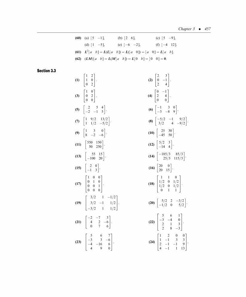
(60) (a) 5 �1½ ], (b) 2 6½ ], (c) 5 �9½ ],
(d) 1 �5½ ], (e) �6 �2½ ], (f) �4 12½ ].
(61) L2 a b½ ] ¼ L(L a b½ ]) ¼ L( a 0½ ]) ¼ a 0½ ] ¼ L a b½ ].
(62) (LM) a b½ ] ¼ L(M a b½ ]) ¼ L 0 b½ ] ¼ 0 0½ ] ¼ 0.
Section 3.3
(1)
1 2
1 0
0 2
24
35. (2)
2 3
0 �1
2 4
24
35.
(3)
1 0
0 2
0 0
24
35. (4)
0 �1
2 4
0 0
24
35.
(5)2 5 4
�2 �1 5
� �. (6)
�1 3 0
�3 �8 9
� �.
(7)1 9=2 13=21 1=2 �5=2
� �. (8)
�5=2 �1 9=23=2 4 �9=2
� �.
(9)1 3 0
8 �2 �6
� �. (10)
25 30
�45 50
� �.
(11)550 150
50 250
� �. (12)
5=2 3
�14 4
� �.
(13)55 15
�100 20
� �. (14)
�185=3 85=325=3 115=3
� �.
(15)2 0
�1 3
� �. (16)
20 0
20 15
� �.
(17)
1 0 0
0 1 0
0 0 1
0 0 0
2664
3775. (18)
1 1 0
1=2 0 1=21=2 0 1=20 1 1
2664
3775.
(19)
3=2 1 �1=2
3=2 �1 1=2
�3=2 1 1=2
264
375. (20)
5=2 2 �3=2�1=2 0 5=2
� �.
(21)
�2 �7 3
4 2 �6
0 7 6
24
35. (22)
5 6 1
�3 �4 0
2 1 3
2 8 �3
2664
3775.
(23)
5 6 7
�3 3 �6
�4 �16 6
4 9 0
2664
3775. (24)
1 2 0 0
1 �1 3 3
2 �1 �1 9
4 �1 1 13
2664
3775.
Chapter 3 . 457

(25)�1=3 0 �13=3 3
2=3 1 11=3 0
� �. (26)
4
�2
6
24
35.
(27)
1
3
�2
24
35. (28)
�2
�8
�6
24
35.
(29)5
23
� �. (30)
8
18
� �.
(31)2
�9
� �. (32)
�65
�240
� �.
(33) 6t� 2. (34) 6t� 2.
(35)0
10
� �. (36)
�4
9
�19
24
35.
(37)
0
�20
28
24
35.
(38) (5a� b� 2a)
(39) (8a� 2b)tþ (13a� 3b).
(40) (4a� bþ 3c)t2 þ (3a� 2bþ 2c)tþ (2a� 2bþ c).
(41)3aþ c 2aþ 2c� 2d
2a� bþ 2c� d a
� �.
Section 3.4
(1)�1 0
1 1
� �. (2)
2 1
�1 0
� �.
(3)�1 1
1 0
� �. (4)
0 1
1 1
� �.
(5)�1 �1
3 4
� �. (6)
�4 �1
3 1
� �.
(7)�10 �10
30 �10
� �. (8) 1
2
1 1 �1
�1 1 1
1 �1 1
24
35.
(9)
1 �1 0
0 1 �1
0 0 1
24
35. (10)
1 1 1
0 1 1
0 0 1
24
35.
(11) 12
1 2 1
�1 0 1
1 0 1
24
35. (12)
1 0 3=20 1 3=20 0 �1=2
24
35.
(13)
0 �1 �2
1 0 2
0 1 1
24
35.
458 . Answers and Hints to Selected Problems

(14) (a)1 5
1 �2
� �, (b)
�4 �5
1 3
� �.
(15) (a)17 23
�13 �18
� �, (b)
1 �1
�5 �2
� �.
(16) (a)2 0
6 5
� �, (b)
5 0
0 2
� �.
(17) (a)�1 0
3 2
� �, (b)
�1 0
0 2
� �.
(18) (a)3 0
0 �1
� �, (b)
15 4
�18 �5
� �.
(19) (a)�13 �6
24 13
� �, (b)
1 6
0 3
� �.
(20) (a)1 0
0 1
� �, (b)
1 0
0 1
� �.
(21) (a)0 0
0 0
� �, (b)
0 0
0 0
� �.
(22) (a)
3 �1 1
2 0 �2
3 �3 1
24
35, (b)
2 0 0
0 �2 0
0 0 2
24
35.
(23) (a)
3 �1 1
2 0 �2
3 �3 1
24
35, (b)
1 2 3
�1 0 �1
3 0 1
24
35.
(24) (a)
1 �1 0
0 2 0
1 0 3
24
35, (b)
1=2 �1 �3=23=2 3 3=2�1=2 0 5=2
24
35.
(25) (a)
1 0 0
0 2 0
0 0 �3
24
35, (b)
1 1 �1
0 2 5
0 0 �3
24
35.
(26) If PA ¼ BP, then P ¼ a b
0 0
� �, which is singular.
(27) If PA ¼ BP, then P ¼ d
3
�2 1
0 3
� �with d arbitrary. Choose d 6¼ 0 to make P
invertible.
(29) Given that transition matrices P1 and P2 exist such that A ¼ P�11 BP1 and
B ¼ P�12 CP2. Then
A ¼ P�11 P�1
2 CP2
� �P1 ¼ A ¼ P�1
1 P�12
� �C P2P1ð Þ ¼ A ¼ P2P1ð Þ�1
C P2P1ð Þ:
Take P ¼ P2P1.
(30) If A ¼ P�1BP, then
A2 ¼ AA ¼ (P�1BP)(P�1BP) ¼ (P�1B)(PP�1)(BP) ¼ (P�1B)I(BP) ¼ P�1B2P:
Chapter 3 . 459

(32) If A ¼ P�1BP, then AT ¼ (P�1BP)T ¼ PTBT(P�1)T ¼ PTBT(PT)�1. Take the new
transition matrix to be PT.
(33) Take P ¼ I.
(35) If A ¼ P�1BP, then B ¼ PAP�1. First show that PA�1P�1 is the inverse of B. Next,
A�1 ¼ (P�1BP)�1 ¼ P�1B�1(P�1)�1 ¼ P�1B�1P.
(36) P can be any invertible 2� 2 matrix.
(37) P can be any invertible 2� 2 matrix.
(38) P ¼
0 1 0 0 . . . 0
0 0 1 0 . . . 0
0 0 0 1 . . . 0
..
. ... ..
. ... ..
.
0 0 0 0 . . . 1
1 0 0 0 . . . 0
26666664
37777775.
Section 3.5(1) (b) and (c).
(2) (b) and (c).
(3) (a), (b), (c), and (d).
(4) (b) and (d).
(5) (d).
(6) (a) 1 0 1½ ], (b) 1 0 �1½ ], (c) 2 0 0½ ], (d) 1 0 2½ ].
(7) (a) Not in the range. (b) 1 0 0½ ],
(c) 2 0 0½ ], (d) Not in the range.
(8) (a) Not in the range, (b)1 0
0 0
� �,
(c) Not in the range, (d)3 0
0 5
� �.
(9) (a)1 1
1 1
� �, (b)
0 0
1 0
� �, (c)
1 0
0 0
� �, (d)
0 �5
3 0
� �.
(10) (a) Not in the range. (b) 2t2 � 2, (c) �3, (d) Not in the range.
(11) Nullity is 0, rank is 2, one-to-one and onto.
(12) Nullity is 0, rank is 2, one-to-one and onto.
(13) Nullity is 1, rank is 1, neither one-to-one nor onto.
(14) Nullity is 1, rank is 2, not one-to-one but onto.
(15) Nullity is 1, rank is 2, not one-to-one but onto.
(16) Nullity is 2, rank is 1, neither one-to-one nor onto.
(17) Nullity is 0, rank is 2, one-to-one but not onto.
(18) Nullity is 0, rank is 2, one-to-one but not onto.
460 . Answers and Hints to Selected Problems

(19) Nullity is 0, rank is 2, one-to-one but not onto.
(20) Nullity is 1, rank is 1, neither one-to-one nor onto.
(21) Nullity is 1, rank is 1, neither one-to-one nor onto.
(22) Nullity is 2, rank is 1, not one-to-one but onto.
(23) Nullity is 3, rank is 0, neither one-to-one nor onto.
(24) Nullity is 0, rank is 4, one-to-one and onto.
(25) Nullity is 2, rank is 2, neither one-to-one nor onto.
(26) Nullity is 3, rank is 1, neither one-to-one nor onto.
(27) Nullity is 3, rank is 1, not one-to-one but onto.
(28) Nullity is 2, rank is 1, neither one-to-one nor onto.
(29) Nullity is 1, rank is 2, neither one-to-one nor onto.
(30) Nullity is 3, rank is 0, neither one-to-one nor onto.
(31) (b) and (d).
(32) (a) and (d).
(33) (b) and (c).
(34)�2
1
� �� �for the kernel;
1
2
� �� �for the range.
(35) The kernel contains only the zero vector; the range is R2.
(36)
1
1
0
2435,
0
0
1
2435
8<:
9=; for the kernel;
1
�1
� �� �for the range.
(37)
0
1
0
2435
8<:
9=; for the kernel; the range is R2.
(38)
�1
�1
1
24
35
8<:
9=; for the kernel;
1
2
3
2435,
0
1
1
2435
8<:
9=; for the range.
(39)
�1
1
0
24
35,
�1
0
1
24
35
8<:
9=; for the kernel;
1
1
1
2435
8<:
9=; for the range.
(40) The kernel contains only the zero vector; the range is R3.
(41) The kernel contains only the zero vector; the range is R1.
(42)
�1
1
0
0
2664
3775,
�2
0
1
0
2664
3775,
�2
0
0
1
2664
3775
8>><>>:
9>>=>>; for the kernel; the range is R1.
(43) They are the same.
Chapter 3 . 461

(44) Rank of T ¼ dimension of W. Use Corollary 1 and the fact that the nullity of T is
nonnegative.
(45) dim (M2�2) ¼ 4 > 3 ¼ dim (P2).
(46) dim (R3) ¼ 3 > 2 ¼ dim (R2).
(47) IfPki¼1
civi ¼ 0, then
0 ¼ T(0) ¼ TPki¼1
civi
¼Pki¼1
ciT(vi) ¼Pki¼1
ciwi , and c1 ¼ c2 ¼ . . . ¼ ck ¼ 0.
(48) If dim (W) < dim (V), then the nullity of V is greater than zero and many vectors
map into the zero vector.
(49) dim (R3) ¼ 3 < 4 ¼ dim (R4).
(50) dim (R3) ¼ 3 < 4 ¼ dim (M2�2).
(51) If w 2 Im(T), then there exists a vector v 2 V such that T(v) ¼ w. Since v ¼Ppi¼1
civi,
it follows that
w ¼ T(v) ¼ TPpi¼1
civi
¼Ppi¼1
ciT(vi).
(52) 0 ¼Pki¼1
ciT(vi) implies that 0 ¼ TPki¼1
civi
. Then
Pki¼1
civi ¼ 0 if T is one-to-one and
c1 ¼ c2 ¼ . . . ¼ cn ¼ 0 if fv1, v2, . . . , vng is linearly independent. Conversely, let
fv1, v2, . . . , vng be a basis for V. This set is linearly independent, and by hypothesis
so is fT(v1), T(v2), . . . , T(vn)g.
If T(u) ¼ T(v), with u ¼Pni¼1
civi and v ¼Pni¼1
divi, thenPni¼1
ciT(vi) ¼ T(u) ¼ T(v) ¼Pni¼1
diT(vi), andPni¼1
ci � dið ÞT(vi) ¼ 0, whereupon
ci � di ¼ 0(i ¼ 1, 2, . . . , n), and u ¼ v.
(53) Let fv1, v2, . . . , vng be a basis for V. We are given that fT(v1), T(v2), . . . , T(vn)g
is a basis for W. If T(u) ¼ T(v), with u ¼Pni¼1
civi and v ¼Pni¼1
divi, then
Pni¼1
ciT(vi) ¼ T(u) ¼ T(v) ¼Pni¼1
diT (vi), and it follows from Theorem 5 of Section
2.4 that u ¼ v.
(54) Let the dimension of V ¼ n. T is one-to-one if and only if v(T) ¼ 0 (Theorem 5) if
and only if the rank of T equals n (Corollary 1) if and only if an n� n matrix
representation of T has rank n if and only if the matrix has an inverse (Theorem 5 of
Section 2.6).
(55) T is onto if and only if T is one-to-one (Theorem 6). Then use the results of
Problem 54.
462 . Answers and Hints to Selected Problems

Chapter 4
Section 4.1(1) (a), (d), (e), (g), and (i).
(2) l ¼ 3 for (a), (e), and (g); l ¼ 5 for (d) and (i).
(3) (b), (c), (d), (e), and (g).
(4) l ¼ 2 for (b); l ¼ 1 for (c) and (d); l ¼ 3 for (e) and (g).
(5) (a), (b), and (d).
(6) l ¼ �2 for (a); l ¼ �1 for (b); l ¼ 2 for (d).
(7) (a), (c), and (d).
(8) l ¼ �2 for (b) and (c); l ¼ 1 for (d).
(9)2
1
� �� �for l ¼ 2;
1
1
� �� �for l ¼ 3.
(10)1
�1
� �� �for l ¼ 1;
1
2
� �� �for l ¼ 4.
(11)3
�2
� �� �for l ¼ 0;
1
2
� �� �for l ¼ 8.
(12)1
�1
� �� �for l ¼ �3;
2
3
� �� �for l ¼ 12.
(13)1
1
� �� �for l ¼ 3;
1
�2
� �� �for l ¼ �3.
(14) No real eigenvalues.
(15)1
0
� �� �for l ¼ 3 with multiplicity 2.
(16)1
0
� �,
0
1
� �� �for l ¼ 3 with multiplicity 2.
(17)1
1
� �� �for l ¼ t;
�1
2
� �� �for l ¼ �2t.
(18)�1
1
� �� �for l ¼ 2u;
�2
1
� �� �for l ¼ 3u.
(19)
0
1
0
2435
8<:
9=; for l ¼ 2;
1
1
1
2435
8<:
9=; for l ¼ 4;
�1
0
1
24
35
8<:
9=; for l ¼ �2.
(20)
1
�4
1
24
35
8<:
9=; for l ¼ 1;
0
1
0
2435
8<:
9=; for l ¼ 2;
�1
0
1
24
35
8<:
9=; for l ¼ 3.
Chapter 4 . 463
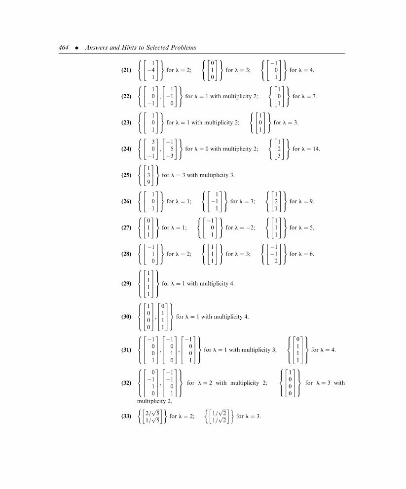
(21)
1
�4
1
24
35
8<:
9=; for l ¼ 2;
0
1
0
2435
8<:
9=; for l ¼ 3;
�1
0
1
24
35
8<:
9=; for l ¼ 4.
(22)
1
0
�1
24
35,
1
�1
0
24
35
8<:
9=; for l ¼ 1 with multiplicity 2;
1
0
1
2435
8<:
9=; for l ¼ 3.
(23)
1
0
�1
24
35
8<:
9=; for l ¼ 1 with multiplicity 2;
1
0
1
2435
8<:
9=; for l ¼ 3.
(24)
3
0
�1
24
35,
�1
5
�3
24
35
8<:
9=; for l ¼ 0 with multiplicity 2;
1
2
3
2435
8<:
9=; for l ¼ 14.
(25)
1
3
9
2435
8<:
9=; for l ¼ 3 with multiplicity 3.
(26)
1
0
�1
24
35
8<:
9=; for l ¼ 1;
1
�1
1
24
35
8<:
9=; for l ¼ 3;
1
2
1
2435
8<:
9=; for l ¼ 9.
(27)
0
1
1
2435
8<:
9=; for l ¼ 1;
�1
0
1
24
35
8<:
9=; for l ¼ �2;
1
1
1
2435
8<:
9=; for l ¼ 5.
(28)
�1
1
0
24
35
8<:
9=; for l ¼ 2;
1
1
1
2435
8<:
9=; for l ¼ 3;
�1
�1
2
24
35
8<:
9=; for l ¼ 6.
(29)
1
1
1
1
26643775
8>><>>:
9>>=>>; for l ¼ 1 with multiplicity 4.
(30)
1
0
0
0
26643775,
0
1
1
1
26643775
8>><>>:
9>>=>>; for l ¼ 1 with multiplicity 4.
(31)
�1
0
0
1
2664
3775,
�1
0
1
0
2664
3775,
�1
0
0
1
2664
3775
8>><>>:
9>>=>>; for l ¼ 1 with multiplicity 3;
0
1
1
1
26643775
8>><>>:
9>>=>>; for l ¼ 4.
(32)
0
�1
1
0
2664
3775,
�1
�1
0
1
2664
3775
8>><>>:
9>>=>>; for l ¼ 2 with multiplicity 2;
1
0
0
0
26643775
8>><>>:
9>>=>>; for l ¼ 3 with
multiplicity 2.
(33)2=
ffiffiffi5p
1=ffiffiffi5p
� �� �for l ¼ 2;
1=ffiffiffi2p
1=ffiffiffi2p
� �� �for l ¼ 3.
464 . Answers and Hints to Selected Problems

(34)1=
ffiffiffi2p
�1=ffiffiffi2p
� �� �for l ¼ 1;
1=ffiffiffi5p
2=ffiffiffi5p
� �� �for l ¼ 4.
(35)3=
ffiffiffiffiffi13p
�2=ffiffiffiffiffi13p
� �� �for l ¼ 0;
1=ffiffiffi5p
2=ffiffiffi5p
� �� �for l ¼ 8.
(36)
0
1
0
2435
8<:
9=; for l ¼ 2;
1=ffiffiffi3p
1=ffiffiffi3p
1=ffiffiffi3p
24
35
8<:
9=; for l ¼ 4;
�1=ffiffiffi2p
0
1=ffiffiffi2p
24
35
8<:
9=; for l ¼ �2.
(37)1=
ffiffiffiffiffi18p
�4=ffiffiffiffiffi18p
1=ffiffiffiffiffi18p
24
35
8<:
9=; for l ¼ 1;
0
1
0
2435
8<:
9=; for l ¼ 2;
�1=ffiffiffi2p
0
1=ffiffiffi2p
24
35
8<:
9=; for l ¼ 3.
(38) �5tþ (3�ffiffiffiffiffi34p
)� �
for l ¼ffiffiffiffiffi34p
; �5tþ (3þffiffiffiffiffi34p
)� �
for l ¼ �ffiffiffiffiffi34p
.
(39) f�5tþ 2g for l ¼ 1; ft� 1g for l ¼ �2.
(40) ft2 þ 1, tg for l ¼ 1; f�t2 � 2tþ 1g for l ¼ 3.
(41)1
�1
� �� �for l ¼ 3 with multiplicity 2.
(42)5
3
� �� �for l ¼ 10;
2
�3
� �� �for l ¼ �11.
(43)
5
�4
1
24
35
8<:
9=; for l ¼ 0;
�1
0
1
24
35
8<:
9=; for l ¼ 2 with multiplicity 2.
(44)
1
0
�1
24
35,
1
2
1
2435
8<:
9=; for l ¼ 2 with multiplicity 2;
1
�1
1
24
35
8<:
9=; for l ¼ 5.
(45)1 1
0 1
� �� �for l ¼ 1 with multiplicity 3.
(46) f1g for l ¼ 0 of multiplicity 2.
(47) ft, 1g for l ¼ 0 of multiplicity 3.
(48) ft, 1g for l ¼ 0 of multiplicity 3.
(49) fe3tg for l ¼ 3; fe�3tg for l ¼ �3.
(50) fe3t, e�3tg for l ¼ 9 of multiplicity 2.
(51) No real eigenvalues.
(52) fsin t , cos tg for l ¼ 1 of multiplicity 2.
(53) fsin 2t, cos 2tg for l ¼ 4 of multiplicity 2.
Chapter 4 . 465

(54) Expanding by the first column,
�l 1 0 . . . 0 00 �l 1 . . . 0 0... ..
. ... . .
. ... ..
.
0 0 0 1 00 0 0 �l 1�a0 �a1 �a2 . . . �an�1 �an � l
������������
������������
¼ �l
�l 1 0 . . . 0 00 �l 1 . . . 0 0... ..
. ... . .
. ... ..
.
0 0 0 . . . �l 1�a1 �a2 �a3 . . . �an�1 �an � l
����������
����������
þ (� 1)na0
1 0 . . . 0 0�l 1 . . . 0 0... ..
. . .. ..
. ...
0 0 1 00 0 . . . �l 1
����������
����������:
Use the induction hypothesis on the first determinant and note that the second
determinant is the determinant of a lower triangular matrix.
Section 4.2(1) 9.
(2) 9.2426.
(3) 5þ 8þ l ¼ �4, l ¼ �17.
(4) (5)(8)l ¼ �4, l ¼ �0:1
(5) Their product is �24.
(6) (a) �6, 8; (b) �15, 20; (c) �6, 1; (d) 1, 8.
(7) (a) 4, 4, 16; (b) �8 ,8, 64; (c) 6,� 6,� 12; (d) 1, 5, 7.
(8) (a) 2A, (b) 5A, (c) A2, (d) Aþ 3I.
(9) (a) 2A, (b) A2, (c) A3, (d) A� 2I.
(10) 8þ 2 ¼ 10 ¼ (5þffiffiffiffiffi18p
)þ (5�ffiffiffiffiffi18p
) ¼ l1 þ l2;
det (A) ¼ 7 ¼ (5þffiffiffiffiffi18p
)(5�ffiffiffiffiffi18p
) ¼ l1l2.
(11) 1þ 2þ 7 ¼ 10 ¼ 0þ (5þffiffiffiffiffi10p
)þ (5�ffiffiffiffiffi10p
) ¼ l1 þ l2 þ l3;
det (A) ¼ 0 ¼ (0)(5þffiffiffiffiffi10p
)(5�ffiffiffiffiffi10p
) ¼ l1l2l3.
(12)1
5þffiffiffiffiffi18p ¼ 1
7(5�
ffiffiffiffiffi18p
) and1
5�ffiffiffiffiffi18p ¼ 1
7(5þ
ffiffiffiffiffi18p
) for Problem 10.
The matrix in Problem 11 has a zero eigenvalue and no inverse.
466 . Answers and Hints to Selected Problems

(13) A ¼ 1 2
4 3
� �has eigenvalues �1 and 5; B ¼ 2 �1
3 �2
� �has eigenvalues
1 and �1; Aþ B ¼ 3 1
7 1
� �has eigenvalues 2 2
ffiffiffi2p
.
(14) Use A and B from the solution to Problem 13. Then AB ¼ 8 �5
14 �10
� �has
eigenvalues �1ffiffiffiffiffi11p
.
(15) x ¼�1
1
� �is an eigenvector of A ¼ 1 2
4 3
� �, but ATx ¼ 1 4
2 3
� ��1
1
� �¼ 3
1
� �6¼ lx for any real constant l.
(16) (A� cI)x ¼ Ax� cx ¼ lx� cx ¼ (l� c)x.
(17) det (AT � lI) ¼ det (A� lI)T ¼ det (A� lI).
(23) (a) A2 � 4A� 5I ¼1 2
4 3
� �1 2
4 3
� �� 4
1 2
4 3
� �� 5
1 0
0 1
� �¼
0 0
0 0
� �:
(b) A2 � 5A ¼1 2
2 4
� �1 2
2 4
� �� 4
1 2
2 4
� �� 5
1 0
0 1
� �¼
0 0
0 0
� �:
(24) Use the results of Problem 18 and Theorem 7 of Appendix A.
(25) An þ an�1An�1 þ a1Aþ a0I ¼ 0
A[An�1 þ an�1An�2 þ þ a1I] ¼ �a0I
or
A[� 1a0
(An�1 þ an�1An�2 þ þ a1I)] ¼ I
Thus, (� 1=a0)(An�1 þ an�1A
n�2 þ þ a1I) is the inverse of A.
(26) (a) A�1 ¼ �2 1
3=2 �1=2
� �, (b) since a0 ¼ 0, the inverse does not exist,
(c) since a0 ¼ 0, the inverse does not exist,
(d) A�1 ¼�1=3 �1=3 2=3�1=3 1=6 1=61=2 1=4 �1=4
24
35, (e) A�1 ¼
1 0 0 0
0 �1 0 0
0 0 �1 0
0 0 0 1
2664
3775.
Section 4.3
(1) Yes; M ¼ 3 1
1 1
� �, D ¼ 1 0
0 �1
� �.
(2) No, if the vector space is the set of real two-tuples. Yes, if the vector space is the set
of two-tuples with complex valued components; then
M ¼2þ i 2� i
1 1
� �, D ¼
i 0
0 �i
� �.
Chapter 4 . 467

(3) No. (4) No.
(5) Yes; M ¼�10 0 0
1 1 �3
8 2 1
24
35, D ¼
1 0 0
0 3 0
0 0 �4
24
35.
(6) Yes; M ¼1 0 1
�2 �2 0
0 1 1
24
35, D ¼
3 0 0
0 3 0
0 0 7
24
35.
(7) Yes; M ¼3 �2 1
0 1 2
�1 0 3
24
35, D ¼
0 0 0
0 0 0
0 0 14
24
35.
(8) Yes; M ¼1 1 1
0 1 �1
�1 0 1
24
35, D ¼
2 0 0
0 2 0
0 0 5
24
35.
(9) No. (10) No. (11) No.
(12) Yes; f3tþ 1, tþ 1g.
(13) Yes; f3tþ 1, �tþ 3g.
(14) Yes; f�10t2 þ tþ 8, tþ 2, � 3tþ 1g.
(15) Yes; ft2 � 2t, � 2tþ 1, t2 þ 1g.
(16) No.
(17) Yes,3 0
0 �1
� ��,�1 5
0 �3
� �,
1 2
0 3
� ��.
(18) No.
(19) Yes,1 0
0 �1
� ��,
1 0
2 1
� �,
1 0
�1 1
� ��.
(20) No.
(21) No.
Section 4.4
(1)e�1 0
0 e4
� �. (2)
e2 0
0 e3
� �.
(3)e�7 0
0 e�7
� �. (4)
1 0
0 1
� �.
(5)e�7 e�7
0 e�7
� �. (6)
e2 e2
0 e2
� �.
(7)e3 e3
0 e3
� �. (8)
1 1
0 1
� �.
(9)e2 0 0
0 e3 0
0 0 e4
24
35. (10)
e1 0 0
0 e�5 0
0 0 e�1
24
35.
468 . Answers and Hints to Selected Problems

(11)e2 0 0
0 e2 0
0 0 e2
24
35. (12)
e2 e2 12e2
0 e2 e2
0 0 e2
24
35.
(13)e�1 e�1 1
2e�1
0 e�1 e�1
0 0 e�1
24
35. (14)
1 1 1
0 1 1
0 0 1
24
35.
(15)e�1 0 0
0 e�1 e�1
0 0 e�1
24
35. (16)
e2 0 0
0 e2 e2
0 0 e2
24
35.
(17)
e1 0 0 0
0 e5 0 0
0 0 e�5 0
0 0 0 e3
2664
3775. (18)
e�5 0 0 0
0 e�5 0 0
0 0 e�5 0
0 0 0 e�5
2664
3775.
(19)
e�5 0 0 0
0 e�5 0 0
0 0 e�5 e�5
0 0 0 e�5
2664
3775. (20)
e�5 0 0 0
0 e�5 e�5 12e�5
0 0 e�5 e�5
0 0 0 e�5
2664
3775.
(21)
e�5 e�5 0 0
0 e�5 0 0
0 0 e�5 e�5
0 0 0 e�5
2664
3775. (22)
e�5 e�5 12e�5 1
6e�5
0 e�5 e�5 12e�5
0 0 e�5 e�5
0 0 0 e�5
2664
3775.
(23)e2 0 e2
0 e2 0
0 0 e2
24
35. (24) 1
7
3e5 þ 4e�2 3e5 � 3e�2
4e5 � 4e�2 4e5 þ 3e�2
� �.
(25) e3 2 �1
1 0
� �. (26) e2
0 1 3
�1 2 5
0 0 1
24
35.
(27) ep
1 p=3 (p2=12)� p
0 1 p=20 0 1
24
35. (28) e2
1 1 1
0 1 2
0 0 1
24
35.
(29)
e 0 0
�eþ 2e2 2e2 �e2
e2 e2 0
24
35.
(30)
e2 e2 0 0
0 e2 0 0
0 0 e3=2=ffiffiffiffiffi27p� �
sinffiffiffiffi27p
2þ
ffiffiffiffiffi27p
cosffiffiffiffi27p
2
�e3=2=
ffiffiffiffiffi27p� �
14 sinffiffiffiffi27p
2
�0 0 e3=2=
ffiffiffiffiffi27p� �
�2 sinffiffiffiffi27p
2
�e3=2=
ffiffiffiffiffi27p� �
� sinffiffiffiffi27p
2þ
ffiffiffiffiffi27p
cosffiffiffiffi27p
2
�
26666664
37777775:
(31) eA ¼ e 3e
0 e
� �and e�A ¼ e�1 �3e�1
0 e�1
� �.
(32) eA ¼12(e8 þ e�8) 1
16(e8 � e�8)
4 (e8 � e�8) 12(e8 þ e�8)
� �and e�A ¼
12(e8 þ e�8) � 1
16(e8 � e�8)
�4(e8 � e�8) 12(e8 þ e�8)
� �.
Chapter 4 . 469

(33) eA ¼1 1 1=20 1 1
0 0 1
24
35 and e�A ¼
1 �1 1=20 1 �1
0 0 1
24
35. A has no inverse.
(34) eA ¼ e e� 1
0 1
� �, eB ¼ 1 e� 1
0 e
� �, eAeB ¼ e 2e2 � 2e
0 e
� �,
eBeA ¼ e 2e� 2
0 e
� �, eAþB ¼ e 2e
0 e
� �.
(35) A ¼ 1 0
0 2
� �, B ¼ 3 0
0 4
� �.
(37) 1=73e8t þ 4et 4e8t � 4et
3e8t � 3et 4e8t þ 3et
� �.
(38)(2=
ffiffiffi3p
) sinhffiffiffi3p
tþ coshffiffiffi3p
t (1=ffiffiffi3p
) sinhffiffiffi3p
t
(� 1=ffiffiffi3p
) sinhffiffiffi3p
t (� 2=ffiffiffi3p
) sinhffiffiffi3p
tþ coshffiffiffi3p
t
� �.
Note: sinhffiffiffi3p
t ¼ effiffi3p
t�e�ffiffi3p
t
2and cosh
ffiffiffi3p
t ¼ effiffi3p
tþe�ffiffi3p
t
2.
(39) e3t 1þ t t
�t 1� t
� �.
(40)1:4e�2t � 0:4e�7t 0:2e�2t � 0:2e�7t
�2:8e�2t þ 2:8e�7t �0:4e�2t þ 1:4e�7t
� �.
(41)0:8e�2t þ 0:2e�7t 0:4e�2t � 0:4e�7t
0:4e�2t � 0:4e�7t 0:2e�2t þ 0:8e�7t
� �.
(42)0:5e�4t þ 0:5e�16t 0:5e�4t � 0:5e�16t
0:5e�4t � 0:5e�16t 0:5e�4t þ 0:5e�16t
� �.
(43) e2t 1 t
0 1
� �. (44)
1 t t2=20 1 t
0 0 1
24
35.
(45) 112
12et 0 0
�9et þ 14e3t � 5e�3t 8e3t þ 4e�3t 4e3t � 4e�3t
�24et þ 14e3t þ 10e�3t 8e3t � 8e�3t 4e3t þ 8e�3t
24
35.
(46) e�t1 t t2=20 1 t
0 0 1
24
35. (47) e4t
1 t 0
0 1 0
0 0 1
24
35.
(48)e2t te2t 0
0 e2t 0
0 0 e�t
24
35. (49) (1=2)
�e�t þ 3et �3e�t þ 3et 0
e�t � et 3e�t � et 0
2tet 2tet 2et
24
35.
(50) e2t
1þ t t 0
�t 1� t 0
t� 12t2 2t� 1
2t2 1
24
35.
(51) et
�2tþ 1 �4t 4tt2
2� 2t t2 � 3tþ 1 �t2 þ 3t
t2
2� 3t t2 � 5t �t2 þ 5tþ 1
24
35
470 . Answers and Hints to Selected Problems

(52)cos (8t) 1
8sin (8t)
�8 sin (8t) cos (8t)
" #.
(53)2 sin (t)þ cos (t) 5 sin (t)
� sin (t) �2 sin (t)þ cos (t)
� �.
(54)1
3e�4t
4 sin (3t)þ 3 cos (3t) sin (3t)
�25 sin (3t) �4 sin (3t)þ 3 cos (3t)
� �.
(55) e4t� sin tþ cos t sin t
�2 sin t sin tþ cos t
� �.
(56)1
3
e�t þ 8e2t 0 4e�t þ 8e2t
3e2t þ 6te2t 6e2t 3e2t þ 6te2t
�e�t � 2e2t 0 �4e�t � 2e2t
264
375
¼ 1
3
�e�t þ 4e2t 0 �4e�t þ 4e2t
3te2t 3e2t 3te2t
e�t � e2t 0 4e�t � e2t
264
375 3 0 4
1 2 1
�1 0 �2
264
375.
(57)� sin t cos t
� cos t � sin t
� �¼
cos t sin t
� sin t cos t
� �0 1
�1 0
� �.
(58) dA2(t)=dt ¼ 2tþ 40t4 6t2 þ 4tet þ 2t2et
16t3 þ 12t2et þ 4t3et 40t4 þ 2e2t
" #,
2A(t)dA(t)=dt ¼ 2tþ 48t4 8t2 þ 4t2et
8t3 þ 24t2et 32t4 þ 2e2t
" #.
Section 4.5(1)
(2)
TABLE
Iteration Eigenvector components Eigenvalue
0 1.0000 1.0000
1 0.6000 1.0000 5.0000
2 0.5238 1.0000 4.2000
3 0.5059 1.0000 4.0476
4 0.5015 1.0000 4.0118
5 0.5004 1.0000 4.0029
TABLE
Iteration Eigenvector components Eigenvalue
0 1.0000 1.0000
1 0.5000 1.0000 10.0000
2 0.5000 1.0000 8.0000
3 0.5000 1.0000 8.0000
Chapter 4 . 471

(3)
(4)
(5)
(6)
TABLE
Iteration Eigenvector components Eigenvalue
0 1.0000 1.0000
1 0.6000 1.0000 15.0000
2 0.6842 1.0000 11.4000
3 0.6623 1.0000 12.1579
4 0.6678 1.0000 11.9610
5 0.6664 1.0000 12.0098
TABLE
Iteration Eigenvector components Eigenvalue
0 1.0000 1.0000
1 0.5000 1.0000 2.0000
2 0.2500 1.0000 4.0000
3 0.2000 1.0000 5.0000
4 0.1923 1.0000 5.2000
5 0.1912 1.0000 5.2308
TABLE
Iteration Eigenvector components Eigenvalue
0 1.0000 1.0000
1 1.0000 0.6000 10.0000
2 1.0000 0.5217 9.2000
3 1.0000 0.5048 9.0435
4 1.0000 0.5011 9.0096
5 1.0000 0.5002 9.0021
TABLE
Iteration Eigenvector components Eigenvalue
0 1.0000 1.0000
1 1.0000 0.4545 11.0000
2 1.0000 0.4175 9.3636
3 1.0000 0.4145 9.2524
4 1.0000 0.4142 9.2434
5 1.0000 0.4142 9.2427
472 . Answers and Hints to Selected Problems

(7)
(8)
(9)
(10)
TABLE
Iteration Eigenvector components Eigenvalue
0 1.0000 1.0000 1.0000
1 0.2500 1.0000 0.8333 12.0000
2 0.0763 1.0000 0.7797 9.8333
3 0.0247 1.0000 0.7605 9.2712
4 0.0081 1.0000 0.7537 9.0914
5 0.0027 1.0000 0.7513 9.0310
TABLE
Iteration Eigenvector components Eigenvalue
0 1.0000 1.0000 1.0000
1 0.6923 0.6923 1.0000 13.0000
2 0.5586 0.7241 1.0000 11.1538
3 0.4723 0.6912 1.0000 11.3448
4 0.4206 0.6850 1.0000 11.1471
5 0.3883 0.6774 1.0000 11.1101
TABLE
Iteration Eigenvector components Eigenvalue
0 1.0000 1.0000 1.0000
1 0.4000 0.7000 1.0000 20.0000
2 0.3415 0.6707 1.0000 16.4000
3 0.3343 0.6672 1.0000 16.0488
4 0.3335 0.6667 1.0000 16.0061
5 0.3333 0.6667 1.0000 16.0008
TABLE
Iteration Eigenvector components Eigenvalue
0 1.0000 1.0000 1.0000
1 0.4000 1.0000 0.3000 �20:0000
2 1.0000 0.7447 0.0284 �14:1000
3 0.5244 1.0000 �0:3683 �19:9504
4 1.0000 0.7168 �0:5303 �18:5293
5 0.6814 1.0000 �0:7423 �20:3976
Chapter 4 . 473

(11)
1
1
1
2435 is a linear combination of
1
�4
1
24
35 and
0
1
0
2435, which are eigenvectors corre-
sponding to l ¼ 1 and l ¼ 2, not l ¼ 3. Thus, the power method converges to
l ¼ 2.
(12) There is no single dominant eigenvalue. Here, jl1j ¼ jl2j ¼ffiffiffiffiffi34p
.
(13) Shift by l ¼ 4. The power method on A ¼ �2 1
2 �1
� �converges after three iter-
ations to m ¼ �3:lþ m ¼ 1.
(14) Shift by l ¼ 16. The power method on A ¼�13 2 3
2 �10 6
3 6 �5
24
35 converges after
three iterations to m ¼ �14: lþ m ¼ 2.
(15)
(16)
(17)
TABLE
Iteration Eigenvector components Eigenvalue
0 1.0000 1.0000
1 �0:3333 1.0000 0.6000
2 1.0000 �0:7778 0.6000
3 �0:9535 1.0000 0.9556
4 1.0000 �0:9904 0.9721
5 �0:9981 1.0000 0.9981
TABLE
Iteration Eigenvector components Eigenvalue
0 1.0000 �0:5000
1 �0:8571 1.0000 0.2917
2 1.0000 �0:9615 0.3095
3 �0:9903 1.0000 0.3301
4 1.0000 �0:9976 0.3317
5 �0:9994 1.0000 0.3331
TABLE
Iteration Eigenvector components Eigenvalue
0 1.0000 1.0000
1 0.2000 1.0000 0.2778
2 �0:1892 1.0000 0.4111
3 �0:2997 1.0000 0.4760
4 �0:3258 1.0000 0.4944
5 �0:3316 1.0000 0.4987
474 . Answers and Hints to Selected Problems

(18)
(19)
(20)
(21)
TABLE
Iteration Eigenvector components Eigenvalue
0 1.0000 1.0000
1 �0:2000 1.0000 0.7143
2 �0:3953 1.0000 1.2286
3 �0:4127 1.0000 1.3123
4 �0:4141 1.0000 1.3197
5 �0:4142 1.0000 1.3203
TABLE
Iteration Eigenvector components Eigenvalue
0 1.0000 1.0000 1.0000
1 1.0000 0.4000 �0:2000 0.3125
2 1.0000 0.2703 �0:4595 0.4625
3 1.0000 0.2526 �0:4949 0.4949
4 1.0000 0.2503 �0:4994 0.4994
5 1.0000 0.2500 �0:4999 0.4999
TABLE
Iteration Eigenvector components Eigenvalue
0 1.0000 1.0000 1.0000
1 0.3846 1.0000 0.9487 �0:1043
2 0.5004 0.7042 1.0000 �0:0969
3 0.3296 0.7720 1.0000 �0:0916
4 0.3857 0.6633 1.0000 �0:0940
5 0.3244 0.7002 1.0000 �0:0907
TABLE
Iteration Eigenvector components Eigenvalue
0 1.0000 1.0000 1.0000
1 �0:6667 1.0000 �0:6667 �1:5000
2 �0:3636 1.0000 �0:3636 1.8333
3 �0:2963 1.0000 �0:2963 1.2273
4 �0:2712 1.0000 �0:2712 1.0926
5 �0:2602 1.0000 �0:2602 1.0424
Chapter 4 . 475

(22) We cannot construct an LU decomposition. Shift as explained in Problem 13.
(23) We cannot solve Lx1 ¼ y uniquely for x1 because one eigenvalue is 0. Shift as
explained in Problem 13.
(24) Yes, on occasion.
(25) Inverse power method applied to A ¼�7 2 3
2 �4 6
3 6 1
24
35 converges to m ¼ 1=6:
lþ 1=m ¼ 10þ 6 ¼ 16.
(26) Inverse power method applied to A ¼27 �17 7
�17 21 1
7 1 11
24
35 converges to m ¼ 1=3:
lþ 1=m ¼ �25þ 3 ¼ �22.
Section 4.6
(1) x(t) ¼ x(t)
y(t)
� �, A(t) ¼ 2 3
4 5
� �, f(t) ¼ 0
0
� �, c ¼ 6
7
� �, t0 ¼ 0.
(2) x(t) ¼ y(t)
z(t)
� �, A(t) ¼ 3 2
4 1
� �, f(t) ¼ 0
0
� �, c ¼ 1
1
� �, t0 ¼ 0.
(3) x(t) ¼ x(t)
y(t)
� �, A(t) ¼ �3 3
4 �4
� �, f(t) ¼ 1
�1
� �, c ¼ 0
0
� �, t0 ¼ 0.
(4) x(t) ¼ x(t)
y(t)
� �, A(t) ¼ 3 0
2 0
� �, f(t) ¼ t
tþ 1
� �, c ¼ 1
�1
� �, t0 ¼ 0.
(5) x(t) ¼ x(t)
y(t)
� �, A(t) ¼ 3 7
1 1
� �, f(t) ¼ 2
2t
� �, c ¼ 2
�3
� �, t0 ¼ 1.
(6) x(t) ¼u(t)
v(t)
w(t)
24
35, A(t) ¼
1 1 1
1 �3 1
0 1 1
24
35, f(t) ¼
0
0
0
2435, c ¼
0
1
�1
24
35, t0 ¼ 4.
(7) x(t) ¼x(t)
y(t)
z(t)
24
35, A(t) ¼
0 6 1
1 0 �3
0 �2 0
24
35, f(t) ¼
0
0
0
2435, c ¼
10
10
20
24
35, t0 ¼ 0.
(8) x(t) ¼r(t)
s(t)
u(t)
24
35, A(t) ¼
1 �3 �1
1 �1 0
2 1 �1
24
35, f(t) ¼
sin t
t2 þ 1
cos t
24
35, c ¼
4
�2
5
24
35, t0 ¼ 1.
(9) x(t) ¼ x1(t)
x2(t)
� �, A(t) ¼ 0 1
3 2
� �, f(t) ¼ 0
0
� �, c ¼ 4
5
� �, t0 ¼ 0.
(10) x(t) ¼ x1(t)
x2(t)
� �, A(t) ¼ 0 1
1 �1
� �, f(t) ¼ 0
0
� �, c ¼ 2
0
� �, t0 ¼ 1.
(11) x(t) ¼ x1(t)
x2(t)
� �, A(t) ¼ 0 1
1 0
� �, f(t) ¼ 0
t2
� �, c ¼ �3
3
� �, t0 ¼ 0.
476 . Answers and Hints to Selected Problems

(12) x(t) ¼ x1(t)
x2(t)
� �, A(t) ¼ 0 1
3 2
� �, f(t) ¼ 0
2
� �, c ¼ 0
0
� �, t0 ¼ 0.
(13) x(t) ¼ x1(t)
x2(t)
� �, A(t) ¼ 0 1
�2 3
� �, f(t) ¼ 0
e�t
� �, c ¼ 2
2
� �, t0 ¼ 1.
(14) x(t) ¼x1(t)
x2(t)
x3(t)
24
35, A(t) ¼
0 1 0
0 0 1
1 0 �1
24
35, f(t) ¼
0
0
0
2435, c ¼
2
1
�205
24
35, t0 ¼ �1.
(15) x(t) ¼
x1(t)
x2(t)
x3(t)
x4(t)
2664
3775, A(t) ¼
0 1 0 0
0 0 1 0
0 0 0 1
0 1 �1 0
2664
3775, f(t) ¼
0
0
0
1
26643775, c ¼
1
2
p
e3
2664
3775, t0 ¼ 0.
(16) x(t) ¼
x1(t)
x2(t)
x3(t)
x4(t)
x5(t)
x6(t)
26666664
37777775, A(t) ¼
0 1 0 0 0 0
0 0 1 0 0 0
0 0 0 1 0 0
0 0 0 0 1 0
0 0 0 0 0 1
0 0 0 0 �4 0
26666664
37777775, f(t) ¼
0
0
0
0
0
t2 � t
26666664
37777775, c ¼
2
1
0
2
1
0
26666664
37777775, t0 ¼ p.
Section 4.7
(3) (a) e�3t1 �t t2=20 1 �t
0 0 1
24
35,
(b) e3(t�2)1 (t� 2) (t� 2)2=20 1 (t� 2)
0 0 1
24
35,
(c) e3(t�s)1 (t� s) (t� s)2=20 1 (t� s)
0 0 1
24
35,
(d) e�3(t�2)1 �(t� 2) (t� 2)2=20 1 �(t� s)
0 0 1
24
35.
(4) (a)1
6
2e�5t þ 4et 2e�5t � 2et
4e�5t � 4et 4e�5t þ 2et
� �, (b)
1
6
2e�5s þ 4es 2e�5s � 2es
4e�5s � 4es 4e�5s þ 2es
� �,
(c)1
6
2e5(t�3) þ 4e�(t�3) 2e5(t�3) � 2e�(t�3)
4e5(t�3) � 4e�(t�3) 4e5(t�3) þ 2e�(t�3)
� �.
(5) (a)1
3
sin 3tþ 3 cos 3t �5 sin 3t
2 sin 3t � sin 3tþ 3 cos 3t
� �,
(b)1
3
sin 3sþ 3 cos 3s �5 sin 3s
2 sin 3s � sin 3sþ 3 cos 3s
� �,
(c)1
3
sin 3(t� s)þ 3 cos 3(t� s) �5 sin 3(t� s)
2 sin 3(t� s) � sin 3(t� s)þ 3 cos 3(t� s
� �.
Chapter 4 . 477

(6) Only (c). (7) Only (c). (8) Only (b).
(9) x(t) ¼ 5e(t�2) � 3e�(t�2), y(t) ¼ 5e(t�2) � e�(t�2).
(10) x(t) ¼ 2e(t�1) � 1, y(t) ¼ 2e(t�1) � 1.
(11) x(t) ¼ k3et þ 3k4e
�t, y(t) ¼ k3et þ k4e
�t.
(12) x(t) ¼ k3et þ 3k4e
�t � 1, y(t) ¼ k3et þ k4e
�t � 1.
(13) x(t) ¼ cos 2t� (1=6) sin 2tþ (1=3) sin t.
(14) x(t) ¼ t4=24þ (5=42 � (2=3þ 3=8.
(15) x(t) ¼ (4=92t þ (5=9�t � (1=3�t.
(16) x(t) ¼ �8 cos t� 6 sin tþ 8þ 6t, y(t) ¼ 4 cos t� 2 sin t� 3.
Section 4.8Note that the units are kg of sugar for problems (1) through (4) and tons of pollution for
problems (5) through (7).
(1) x(t) ¼ 500e�7t=100(� 1þ e7t=100)
y(t) ¼ 5 e�7t=100(� 100� 7tþ 100e7t=100)
(2) x(t)! 500, y(t)! 437:5 (kg of sugar)
(3) x(t)! 500, y(t)! 583:333 (kg of sugar)
(4) x(t)! 500, y(t)! 500 (kg of sugar)
(5) x(t) ¼ 1
14e�6t(� 1� 7e6t þ 8e7t)
y(t) ¼ 2
21e�6t(� 1þ et)2(1þ 2et þ 3e2t þ 4e3t þ 5e4t þ 6e5t)
x(t)!1, y(t)!1 as t!1
(6) x(t) ¼ 1
14e�6t(� 1� 7e6t þ 8e7t)
y(t) ¼ �2
21e�6t(� 1þ et)2(1þ 2et þ 3e2t þ 4e3t þ 5e4t þ 6e5t)
x(t)!1, y(t)! �1 as t!1 (Note that this is not a realistic model, due to the
behavior of y(t).)
(7) x(t)!1, y(t)!1 as t!1.
Chapter 5
Section 5.1(1) (a) 11, (b)
ffiffiffi5p
, (c) no.
(2) (a) 0, (b)ffiffiffi2p
, (c) yes.
(3) (a) �50, (b)ffiffiffiffiffi74p
, (c) no.
(4) (a) 0, (b)ffiffiffiffiffi68p
, (c) yes.
478 . Answers and Hints to Selected Problems

(5) (a) 0, (b) 5, (c) yes.
(6) (a) 6, (b)ffiffiffi5p
, (c) no.
(7) (a) 26, (b)ffiffiffiffiffi24p
, (c) no.
(8) (a) �30, (b)ffiffiffiffiffi38p
, (c) no.
(9) (a) 0, (b)ffiffiffiffiffiffiffiffiffiffi1400p
, (c) yes.
(10) (a) 7/24, (b)
ffiffiffiffiffi21p
8, (c) no.
(11) (a) 2, (b)ffiffiffi3p
, (c) no.
(12) (a) 0, (b)ffiffiffi3p
, (c) yes.
(13) (a) 0, (b)ffiffiffi2p
, (c) yes.
(14) (a) 1, (b) 1, (c) no.
(15) (a) 1/12, (b)
ffiffiffi3p
2, (c) no.
(16) (a) �13, (b)ffiffiffiffiffi55p
, (c) no.
(17) Inner product undefined.
(18) (a) 3=5 4=5½ �T,
(b) 20=ffiffiffiffiffiffiffiffi425p
5=ffiffiffiffiffiffiffiffi425p� �T
,
(c) 1=ffiffiffiffiffi21p
2=ffiffiffiffiffi21p
4=ffiffiffiffiffi21p� �T
,
(d) �4=ffiffiffiffiffi34p
3=ffiffiffiffiffi34p
�3=ffiffiffiffiffi34p� �T
,
(e)ffiffiffi3p
=3ffiffiffi3p
=3ffiffiffi3p
=3� �T
,
(f) 1=ffiffiffi5p
2=ffiffiffiffiffi55p
3=ffiffiffiffiffi55p
4=ffiffiffiffiffi55p
5=ffiffiffiffiffi55p� �T
.
(19) 36.98. (20) 14.08. (21) 78.78.
(22) 908. (23) 118.58. (24) 50.88.
(25) 19.58. (26) 17.78.
(27) No vector x exists.
(28) With x ¼ [ x1 x2 x3 . . . xn ]T and y ¼ [ y1 y2 y3 . . . yn ]T,
hlx,yi ¼ (lx1)(y1)þ (lx2)(y2)þ . . .þ (lxn)(yn)
¼ l[x1y1 þ x2y2 þ x3y3 þ . . .þ xnyn] ¼ lhx,yi:
(29) * x1
x2
..
.
xn
26664
37775þ
z1
z2
..
.
zn
26664
37775,
y1
y2
..
.
yn
26664
37775+¼
*x1 þ z1
x2 þ z2
..
.
xn þ zn
26664
37775,
y1
y2
..
.
yn
26664
37775+
¼ (x1 þ z1)y1 þ (x2 þ z2)y2 þ . . . (xn þ zn)yn
¼ (x1y1þx2y2þ . . .þxnyn)þ (z1y1þz2y2þ . . .þ znyn)
¼hx,yiþhz,yi
Chapter 5 . 479

(30) h0,yi ¼ h00,yi ¼ 0h0,yi ¼ 0.
(31) jjxþ yjj2 ¼ hxþ y,xþ yi ¼ hx,xi þ hx,yi þ hy,xi þ hy,yi¼ hx,xi þ 0þ 0þ hy,yi ¼ jjxjj2 þ jjyjj2:
(32) jjxþ yjj2 þ jjx� yjj2 ¼ hxþ y,xþ yi þ hx� y,x� yi¼ [hx,xi þ hx,yi þ hy,xi þ hy,yi]þ [hx,xi � hx,yi � hy,xi þ hy,yi]¼ 2hx,xi þ 2hy,yi ¼ 2jjxjj2 þ 2jjyjj2
(33) jjxþ yjj2 � jjx� yjj2 ¼ hxþ y,xþ yi � hx� y,x� yi¼ [hx,xi þ hx,yi þ hy,xi þ hy,yi]� [hx,xi � hx,yi � hy,xi þ hy,yi]¼ 2hx,yi þ 2hy,xi ¼ 4hx,yi
(34) hx,ayþ bzi ¼ hayþ bz,xi ¼ hay,xi þ hbz,xi ¼ ahy,xi þ bhz,xi¼ a(0)þ b(0) ¼ 0
(35) 0 � jjlxþ yjj2 ¼ hlxþ y,lxþ yi¼ hlx,lxi � hlx,yi � hy,lxi þ hy,yi¼ l2hx,xi � lhx,yi � lhy,xi þ hy,yi
(37) From Problem 35, 0 ¼ jjlx� yjj2 if and only if lx� y ¼ 0 if and only if y ¼ lx.
(38) (a) 48.28, (b) 121.48, (c) 1808, (d) 32.68, (e) 26.08.
(40) (a) 44, (b) �23, (c) �17, (d) �12, (e) �11, (f) 53.
(41) (a) 28, (b) �11:5, (c) �6.
(43) 145. (44) 27. (45) 32.
(47) (a) �8, (b) �5, (c) 7, (d) 3, (e) 2, (f) 1.
(48) (a) �22, (b) �184, (c) 22, (d) �21.
(50) (a) �763=60, (b) 325/6, (c) 107/30, (d) 113/6, (e) 303/70, (f) 2.
Section 5.2
(1) (a)1:60:8
� �, (b)
�0:61:2
� �.
(2) (a)0:7059
1:1765
� �, (b)
0:2941
�0:1765
� �.
(3) (a)0:50:5
� �, (b)
2:5�2:5
� �.
(4) (a)0
0
� �, (b)
4
�1
� �.
(5) (a)�0:7529
�3:3882
� �, (b)
�6:2471
1:3882
� �.
(6) (a)
1
0
1
2435, (b)
1
1
�1
24
35.
480 . Answers and Hints to Selected Problems
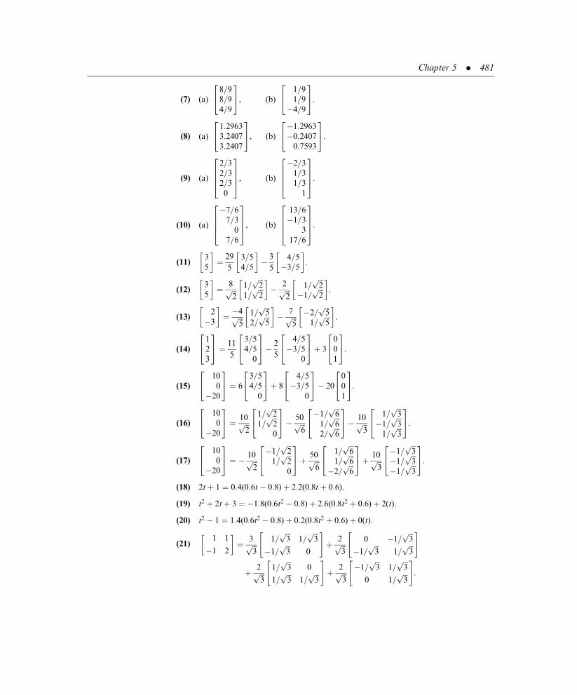
(7) (a)
8=98=94=9
24
35, (b)
1=91=9�4=9
24
35.
(8) (a)
1:2963
3:2407
3:2407
24
35, (b)
�1:2963
�0:2407
0:7593
24
35.
(9) (a)
2=32=32=30
2664
3775, (b)
�2=31=31=3
1
2664
3775.
(10) (a)
�7=67=3
0
7=6
2664
3775, (b)
13=6�1=3
3
17=6
2664
3775.
(11)3
5
� �¼ 29
5
3=54=5
� �� 3
5
4=5�3=5
� �.
(12)3
5
� �¼ 8ffiffiffi
2p 1=
ffiffiffi2p
1=ffiffiffi2p
� �� 2ffiffiffi
2p 1=
ffiffiffi2p
�1=ffiffiffi2p
� �.
(13)2
�3
� �¼ �4ffiffiffi
5p 1=
ffiffiffi5p
2=ffiffiffi5p
� �� 7ffiffiffi
5p �2=
ffiffiffi5p
1=ffiffiffi5p
� �.
(14)
1
2
3
2435 ¼ 11
5
3=54=5
0
24
35� 2
5
4=5�3=5
0
24
35þ 3
0
0
1
2435.
(15)
10
0
�20
24
35 ¼ 6
3=54=5
0
24
35þ 8
4=5�3=5
0
24
35� 20
0
0
1
2435.
(16)
10
0
�20
24
35 ¼ 10ffiffiffi
2p
1=ffiffiffi2p
1=ffiffiffi2p
0
24
35� 50ffiffiffi
6p
�1=ffiffiffi6p
1=ffiffiffi6p
2=ffiffiffi6p
24
35� 10ffiffiffi
3p
1=ffiffiffi3p
�1=ffiffiffi3p
1=ffiffiffi3p
24
35.
(17)
10
0
�20
24
35 ¼ � 10ffiffiffi
2p
�1=ffiffiffi2p
1=ffiffiffi2p
0
24
35þ 50ffiffiffi
6p
1=ffiffiffi6p
1=ffiffiffi6p
�2=ffiffiffi6p
24
35þ 10ffiffiffi
3p
�1=ffiffiffi3p
�1=ffiffiffi3p
�1=ffiffiffi3p
24
35.
(18) 2tþ 1 ¼ 0:4(0:6t� 0:8)þ 2:2(0:8tþ 0:6).
(19) t2 þ 2tþ 3 ¼ �1:8(0:6t2 � 0:8)þ 2:6(0:8t2 þ 0:6)þ 2(t).
(20) t2 � 1 ¼ 1:4(0:6t2 � 0:8)þ 0:2(0:8t2 þ 0:6)þ 0(t).
(21)1 1
�1 2
� �¼ 3ffiffiffi
3p 1=
ffiffiffi3p
1=ffiffiffi3p
�1=ffiffiffi3p
0
" #þ 2ffiffiffi
3p 0 �1=
ffiffiffi3p
�1=ffiffiffi3p
1=ffiffiffi3p
" #
þ 2ffiffiffi3p 1=
ffiffiffi3p
0
1=ffiffiffi3p
1=ffiffiffi3p
" #þ 2ffiffiffi
3p �1=
ffiffiffi3p
1=ffiffiffi3p
0 1=ffiffiffi3p
" #:
Chapter 5 . 481

(22)1 2
3 4
� �¼ 11
5
3=5 4=5
0 0
� �� 2
5
4=5 �3=5
0 0
� �
� 7
5
0 0
3=5 �4=5
� �� 24
5
0 0
�4=5 �3=5
� �:
(23)4 5
�6 7
� �¼ 9� 6
ffiffiffi2p
2
1=2 1=2
1=ffiffiffi2p
0
� �� 9þ 6
ffiffiffi2p
2
�1=2 �1=2
1=ffiffiffi2p
0
� �
þ 1þ 7ffiffiffi2p
2
�1=2 1=2
0 1=ffiffiffi2p
� �� 1� 7
ffiffiffi2p
2
1=2 �1=2
0 1=ffiffiffi2p
� �:
(24)1=
ffiffiffi5p
2=ffiffiffi5p
� �,
2=ffiffiffi5p
�1=ffiffiffi5p
� �. (25)
1=ffiffiffi2p
1=ffiffiffi2p
� �,�1=
ffiffiffi2p
1=ffiffiffi2p
� �.
(26)3=
ffiffiffiffiffi13p
�2=ffiffiffiffiffi13p
� �,
2=ffiffiffiffiffi13p
3=ffiffiffiffiffi13p
� �. (27)
1=ffiffiffi6p
2=ffiffiffi6p
1=ffiffiffi6p
24
35,
1=ffiffiffi3p
�1=ffiffiffi3p
1=ffiffiffi3p
24
35,�1=
ffiffiffi2p
0
1=ffiffiffi2p
24
35.
(28)2=
ffiffiffi5p
1=ffiffiffi5p
0
24
35,�2=
ffiffiffiffiffi45p
4=ffiffiffiffiffi45p
5=ffiffiffiffiffi45p
24
35,
1=3�2=3
2=3
24
35. (29)
1=ffiffiffi2p
1=ffiffiffi2p
0
24
35,
1=ffiffiffi3p
�1=ffiffiffi3p
1=ffiffiffi3p
24
35,�1=
ffiffiffi6p
1=ffiffiffi6p
2=ffiffiffi6p
24
35.
(30)
0
3=54=5
24
35,
3=516=25
�12=25
24
35,
4=5�12=25
9=25
24
35.
(31)
0
1=ffiffiffi3p
1=ffiffiffi3p
1=ffiffiffi3p
2664
3775,
3=ffiffiffiffiffi15p
�2=ffiffiffiffiffi15p
1=ffiffiffiffiffi15p
1=ffiffiffiffiffi15p
2664
3775,
3=ffiffiffiffiffi35p
3=ffiffiffiffiffi35p
�4=ffiffiffiffiffi35p
1=ffiffiffiffiffi35p
2664
3775,
1=ffiffiffi7p
1=ffiffiffi7p
1=ffiffiffi7p
�2=ffiffiffi7p
2664
3775:
(32)
1=ffiffiffi2p
1=ffiffiffi2p
0
0
2664
3775,
�1=ffiffiffi6p
1=ffiffiffi6p
�2=ffiffiffi6p
0
2664
3775,
1=ffiffiffi3p
�1=ffiffiffi3p
�1=ffiffiffi3p
0
2664
3775,
0
0
0
�1
2664
3775.
(33) One of the q vectors becomes zero.
(34) a,x� ha,xiha,ai a
� �¼ ha,xi � a,
ha,xiha,ai a
� �¼ ha,xi � ha,xi
ha,ai ha,ai ¼ 0.
(35) jjsxþ tyjj2 ¼ hsxþ ty,sxþ tyi ¼ s2hx,xi þ 2sthx,yi þ t2hy,yi¼ s2(1)þ st(0)þ t2(1):
(36) An identity matrix.
(37) Set y ¼ x and use part (a) of Theorem 1 of Section 5.1.
(38) Denote the columns of A as A1, A2, . . . , An, and the elements of y as y1, y2, . . . , yn,
respectively. Then, Ay ¼ A1y1 þ A2y2 þ þ Anyn and hAy,pi ¼ y1hA1,piþy2hA2,pi þ þ ynhAn,pi.
(39) Use Theorem 1.
482 . Answers and Hints to Selected Problems

Section 5.3
(1)0:4472 0:8944
0:8944 �0:4472
� �2:2361 1:7889
0:0000 1:3416
� �.
(2)0:7071 �0:7071
0:7071 0:7071
� �1:4142 5:6569
0:0000 1:4142
� �.
(3)0:8321 0:5547
�0:5547 0:8321
� �3:6056 0:8321
0:0000 4:1603
� �:
(4)
0:3333 0:8085
0:6667 0:1617
0:6667 �0:5659
264
375 3:0000 2:6667
0:0000 1:3744
� �.
(5)
0:3015 �0:2752
0:3015 �0:8808
0:9045 0:3853
264
375 3:3166 4:8242
0:0000 1:6514
� �.
(6)
0:7746 0:4034
�0:5164 0:5714
0:2582 0:4706
�0:2582 0:5378
26664
37775 3:8730 0:2582
0:0000 1:9833
� �.
(7)
0:8944 �0:2981 0:3333
0:4472 0:5963 �0:6667
0:0000 0:7454 0:6667
264
375 2:2361 0:4472 1:7889
0:0000 1:3416 0:8944
0:0000 0:0000 2:0000
264
375.
(8)
0:7071 0:5774 �0:4082
0:7071 �0:5774 0:4082
0:0000 0:5774 0:8165
264
375 1:4142 1:4142 2:8284
0:0000 1:7321 0:5774
0:0000 0:0000 0:8165
264
375.
(9)
0:00 0:60 0:80
0:60 0:64 �0:48
0:80 �0:48 0:36
264
375 5 3 7
0 5 2
0 0 1
264
375.
(10)
0:0000 0:7746 0:5071
0:5774 �0:5164 0:5071
0:5774 0:2582 �0:6761
0:5774 0:2582 0:1690
26664
37775
1:7321 1:1547 1:1547
0:0000 1:2910 0:5164
0:0000 0:0000 1:1832
264
375.
(11)
0:7071 �0:4082 0:5774
0:7071 0:4082 �0:5774
0:0000 �0:8165 �0:5774
0:0000 0:0000 0:0000
26664
37775
1:4142 0:7071 0:7071
0:0000 1:2247 0:4082
0:0000 0:0000 1:1547
264
375.
(12) QR 6¼ A.
Chapter 5 . 483

(13) A1 ¼ R0Q0 þ 7I
¼19:3132 �1:2945 0:0000
0:0000 7:0231 �0:9967
0:0000 0:0000 0:0811
264
375 �0:3624 0:0756 0:9289
0:0000 �0:9967 0:0811
0:9320 0:0294 0:3613
264
375
þ 7
1 0 0
0 1 0
0 0 1
264
375 ¼ 0:0000 2:7499 17:8357
�0:9289 �0:0293 0:2095
0:0756 0:0024 7:0293
264
375
(14) A1 ¼ R0Q0 � 14I
¼24:3721 �17:8483 3:8979
0:0000 8:4522 �4:6650
0:0000 0:0000 3:6117
264
375 0:6565 �0:6250 0:4223
�0:6975 �0:2898 0:6553
0:2872 0:7248 0:6262
264
375
� 14
1 0 0
0 1 0
0 0 1
264
375 ¼ 15:5690 �7:2354 1:0373
�7:2354 �19:8307 2:6178
1:0373 2:6178 �11:7383
264
375
(15) Shift by 4.
R0 ¼
4:1231 �0:9701 0:0000 13:5820
0:0000 4:0073 �0:9982 �4:1982
0:0000 0:0000 4:0005 12:9509
0:0000 0:0000 0:0000 3:3435
26664
37775
Q0 ¼
�0:9701 �0:2349 �0:0586 �0:0151
0:2425 �0:9395 �0:2344 �0:0605
0:0000 0:2495 �0:9376 �0:2421
0:0000 0:0000 0:2500 �0:9683
26664
37775
A1 ¼ R0Q0 þ 4I ¼
�0:2353 �0:0570 3:3809 �13:1545
0:9719 �0:0138 �1:0529 4:0640
0:0000 0:9983 3:4864 �13:5081
0:0000 0:0000 0:8358 0:7626
26664
37775
(16) 7:2077,� 0:1039 1:5769i. (17) �11,� 22, 17. (18) 2, 3, 9.
(19) Method fails. A0 � 7I does not have linearly independent columns, so no QR
decomposition is possible.
(20) 2, 2, 16. (21) 1, 3, 3. (22) 2, 3 i. (23) 1, i.
(24) i, 2 3i. (25) 3:1265 1:2638i,� 2:6265 0:7590i.
(26) 0.0102, 0.8431, 3.8581, 30.2887.
(27) Each diagonal element of the upper triangular matrix R is the magnitude of a
nonzero vector (see Theorem 3 of Section 5.2) and is, therefore, nonzero. Use
Theorems 4 and 10 of Appendix A.
484 . Answers and Hints to Selected Problems

(28) QTQ ¼ I. Thus, QT ¼ Q�1.
(29) AkRk�1 ¼ Rk�1Qk�1Rk�1 ¼ Rk�1Ak�1.
Set P ¼ (Rk�1)�1 and use Theorem 1 of Section 4.1.
Section 5.4(1) x � 2:225, y � 1:464. (2) x ¼ 3, y � 3:25.
(3) x � 9:879, y � 18:398. (4) x � �1:174, y � 8:105.
(5) x � 1:512, y � 0:639, z � 0:945. (6) x � 7:845, y � 1:548, z � 5:190.
(7) x � 81:003, y � 50:870, z � 38:801.
(8) x � 2:818, y � �0:364, z � �1:364.
(9) 2 and 4.
(10) (b) y ¼ 2:3xþ 8:1, (c) 21.9.
(11) (b) y ¼ �2:56xþ 54:39, (c) 31 in week 9, 29 in week 10.
(12) (b) y ¼ 0:27xþ 10:24, (c) 12.4.
(13) m ¼NPNi¼1
xiyi �PNi¼1
xi
PNi¼1
yi
NPNi¼1
x2i �
PNi¼1
xi
2, c ¼
PNi¼1
yi
PNi¼1
x2i �
PNi¼1
xi
PNi¼1
xiyi
NPNi¼1
x2i �
PNi¼1
xi
2.
If NPN
i¼1 x2i is near
PNi¼1 xi
�2
, then the denominator is near 0.
(14)PN
i¼1 x0i ¼ 0, so the denominators for m and c found in Problem 13 reduce to
NPN
i¼1 x0i�
)2.
(15) y ¼ 2:3x0 þ 15.
(16) y ¼ �2:56x0 þ 42:88.
(17) (a) y ¼ �0:198x0 þ 21:18, (b) year 2000 is coded as x0 ¼ 30; y(30) ¼ 15:24.
(23) E ¼0:842
0:211
�2:311
24
35. (24) E ¼
0:161
0:069
�0:042
�0:172
2664
3775.
Section 5.5
(1) (a) span
1
0
0
2435,
0
�1
1
24
35
8<:
9=;, (b)
0
1=21=2
24
35.
(2) (a) span
�1
1
0
24
35,
�1
0
1
24
35
8<:
9=;, (b)
2=32=32=3
24
35.
(3) (a) span
�1
2
0
24
35,
�1
0
2
24
35
8<:
9=;, (b)
1
1=21=2
24
35.
Chapter 5 . 485

(4) (a) span
1
�2
1
24
35
8<:
9=;, (b)
7=64=61=6
24
35.
(5) (a) span
1
�4
2
24
35
8<:
9=;, (b)
8=73=72=7
24
35.
(6) (a) span
1
0
0
2435
8<:
9=;, (b)
0
1
0
2435.
(7) (a) span
�1
1
0
24
35
8<:
9=;, (b)
1
1
0
2435.
(8) Same as Problem 2.
(9) (a) span
0
�1
1
24
35
8<:
9=;, (b)
1
1=21=2
24
35.
(10) (a) f0g, (b)
1
1
0
2435.
(11) (a) span
1
0
0
0
26643775,
0
1
0
0
26643775,
0
0
�1
1
2664
3775
8>><>>:
9>>=>>;, (b)
0
0
1=21=2
2664
3775.
(12) (a) span
1
0
0
0
26643775,
0
�1
1
0
2664
3775,
0
�1
0
1
2664
3775
8>><>>:
9>>=>>;, (b)
0
1=31=31=3
2664
3775.
(13) (a) span
1
0
0
0
26643775,
0
0
�1
1
2664
3775
8>><>>:
9>>=>>;, (b)
0
0
1=21=2
2664
3775.
(14) (a) span
1
0
0
0
26643775,
0
0
1
0
26643775
8>><>>:
9>>=>>;, (b)
0
0
0
0
26643775.
(15) (a) span
�1
1
0
0
2664
3775,
�1
0
1
1
2664
3775
8>><>>:
9>>=>>;, (b)
3=53=54=5�1=5
2664
3775.
(16) (a) span
�2
1
1
1
2664
3775
8>><>>:
9>>=>>;, (b)
5=71=78=71=7
2664
3775.
486 . Answers and Hints to Selected Problems

(17) (a) span
�1
1
0
0
2664
3775,
�1
0
1
0
2664
3775
8>><>>:
9>>=>>;, (b)
2=32=32=30
2664
3775.
(18) (a) span
1
�1
�1
1
2664
3775
8>><>>:
9>>=>>;, (b)
1
0
1
0
26643775.
(19) (a) f0g, (b)
1
0
1
0
26643775.
(20) (a) span
0
�1
1
1
2664
3775
8>><>>:
9>>=>>;, (b)
1
1=32=3�1=3
2664
3775.
(21) No.
(22) jjxjj2 ¼ huþ u?, uþ u?i ¼ hu, ui þ hu, u?i þ hu?, ui þ hu?, u?i¼ hu, ui þ 0þ 0þ hu?, u?i ¼ jjujj2 þ jju?jj2:
(23) Let B ¼ fu1, u2, . . . , urg and C ¼ fw1, w2, . . . , wsg. If v 2 V, then there exists a
u 2 U and w 2W such that v ¼ uþ w. But u ¼Pri¼1
ciui and w ¼Psj¼1
djwj for scalars
c1, . . . , cr, and d1, . . . , ds. Then, v ¼Pri¼1
ciui þPsj¼1
djwj and B [ C is a spanning set
for V. Consider the equationPri¼1
ciui þPsj¼1
djwj ¼ 0. SincePri¼1
(0)ui þPsj¼1
(0)wj ¼ 0, it
follows from uniqueness that ci ¼ 0(i ¼ 1, 2, . . . , r) and dj ¼ 0( j ¼ 1, 2, . . . , s).
Thus, B [ C is linearly independent.
(24) Let v 2 U with basis B ¼ fu1, u2, . . . , urg. Then v ¼Pri¼1
ciui for scalars c1, . . . , cr.
Let v 2W with basis C ¼ fw1, w2, . . . , wsg. Then v ¼Psj¼1
djwj for scalars d1, . . . , ds.
0 ¼ v� v ¼Pri¼1
ciui �Psj¼1
djwj . But 0 ¼Pri¼1
(0)ui �Psj¼1
(0)wj , so it follows from
uniqueness that ci ¼ 0(i ¼ 1, 2, . . . , r) and dj ¼ 0(j ¼ 1, 2, . . . , s). Thus,
v ¼Pri¼1
ciui ¼Pri¼1
(0)ui ¼ 0.
(25) Use the results of Problem 23.
Chapter 5 . 487

Appendices
Appendix A(1) �2. (2) 38. (3) 38. (4) �2.
(5) 82. (6) �82. (7) 9. (8) �20.
(9) 21. (10) �6. (11) 22. (12) 0.
(13) �9. (14) �33. (15) 15. (16) �5.
(17) �10. (18) 0. (19) 0. (20) 0.
(21) 119. (22) �8. (23) 22. (24) �7.
(25) �40. (26) 52. (27) 25. (28) 0.
(29) 0. (30) �11. (31) 0.
(32) 0 and 2. (33) �1 and 4. (34) 2 and 3.
(35) ffiffiffi6p
. (36) l2 � 9l� 2.
(37) l2 � 9lþ 38. (38) l2 � 13l� 2.
(39) l2 � 8lþ 9. (40) �l3 þ 7lþ 22.
(41) �l3 þ 4l2 � 17l. (42) �l3 þ 6l� 9.
(43) �l3 þ 10l2 � 22l� 33.
(44) jAj ¼ 11, jBj ¼ 5, jABj ¼ 55.
(45) 3. (46) 24. (47) 28.
(48) 6 ¼ det9 �6
13 �8
� ��������� ¼ j � 2jj � 3j ¼ det
3 4
5 6
� ��������� det
�1 2
3 �3
� ���������.
(49) 114 ¼ det�15 18
13 �8
� ��������� ¼ 38j � 3j ¼ det
3 �4
5 6
� ��������� det
�1 2
3 �3
� ���������.
(50) 912 ¼ det23 4
�25 �44
� ��������� ¼ 38j � 24j ¼ det
3 �4
5 6
� ��������� det
1 �4
�5 �4
� ���������.
(51) (a) 1, (b) 0, (c) 0.
(52) If the columns are linearly independent, then the parallelpiped generated by the
three vectors collapses into either a parallelogram, a line segment, or the origin
(Theorem 4 of Section 2.4), all of which have zero volume.
(53) It is the product of the diagonal elements.
(54) It must be zero.
(55) �1. (56) 0. (57) �311. (58) �10. (59) 0.
(60) �5. (61) 0. (62) 0. (63) 119. (64) �9.
(65) �33. (66) 15. (67) 2187. (68) 52. (69) 25.
(70) 0. (71) 0. (72) 152.
488 . Answers and Hints to Selected Problems

(73) Multiply the first row by 2, the second row by �1, and the second column by 2.
(74) Apply the third elementary row operation with the third row to make the first two
rows identical.
(75) Multiply the first column by 1/2, the second column by 1/3, to obtain identical
columns.
(76) Interchange the second and third rows, and then transpose.
(77) Use the third column to simplify both the first and second columns.
(78) Factor the numbers �1, 2, 2, and 3 from the third row, second row, first column,
and second column, respectively.
(79) Factor a 5 from the third row. Then use this new third row to simplify the second
row and the new second row to simplify the first row.
(81) det 31 3
�3 4
� �� �¼ 3 9
�9 12
�������� ¼ 117 ¼ 9(13) ¼ (3)2
1 3
�3 4
��������.
(82) det �22 3
�3 �2
� �� �¼ �4 �6
6 4
�������� ¼ 20 ¼ 4(5) ¼ (�2)2
2 3
�3 �2
��������.
(83) det �1
1 2 �2
1 3 3
2 5 0
24
35
8<:
9=; ¼
�1 �2 2
�1 �3 �3
�2 �5 0
������������ ¼ 1 ¼ (�1)(�1) ¼ (�1)3
1 2 �2
1 3 3
2 5 0
������������.
(84) That row can be transformed into a zero row using elementary row operations.
(85) Transform the matrix to row-reduced form by elementary row operations; at least
one row will be zero.
(86) Use Theorem 1 and Theorem 10 of this section.
(87) (1þ 2þ . . .þ n)þ (nþ 1) ¼ n(nþ 1)=2þ (nþ 1) ¼ (nþ 1)(nþ 2)=2.
(88) [1þ 3þ 5þ . . .þ (2n� 1)]þ (2nþ 1) ¼ n2 þ (2nþ 1) ¼ (nþ 1)2.
(89) (12 þ 22 þ . . .þ n2)þ (nþ 1)2
¼ n(nþ 1)(2nþ 1)=6þ (nþ 1)2
¼ (nþ 1)[n(2nþ 1)=6þ (nþ 1)]
¼ (nþ 1)[2n2 þ 7nþ 6]=6
¼ (nþ 1)(nþ 2)(2nþ 3)=6
(90) (13 þ 23 þ . . .þ n3)þ (nþ 1)3
¼ n2(nþ 1)2=4þ (nþ 1)3
¼ (nþ 1)2[n2=4þ (nþ 1)]
¼ (nþ 1)2(nþ 2)2=4.
(91) [12 þ 32 þ 52 þ . . .þ (2n� 1)2]þ (2nþ 1)2
¼ n(4n2 � 1)=3þ (2nþ 1)2
Appendix A . 489

¼ n(2n� 1)(2nþ 1)=3þ (2nþ 1)2
¼ (2nþ 1)[n(2n� 1)=3þ (2nþ 1)]
¼ (2nþ 1)(2nþ 3)(nþ 1)=3
¼ [2(nþ 1)� 1][2(nþ 1)þ 1](nþ 1)=3
¼ [4(nþ 1)2 � 1](nþ 1)=3
(92)Pnþ1
k¼1
3k2 � k� �
¼Pnk¼1
3k2 � k� �
þ [3(nþ 1)2 � (nþ 1)]
¼ n2(nþ 1)þ [3(nþ 1)2 þ (nþ 1)]
¼ (nþ 1)[n2 þ 3(nþ 1)þ 1]
¼ (nþ 1)(nþ 2)(nþ 1)
¼ (nþ 1)2(nþ 2)
(93)Xnþ1
k¼1
1
k(kþ 1)
¼Xn
k¼1
1
k(kþ 1)þ 1
(nþ 1)(nþ 2)
¼ n
nþ 1þ 1
(nþ 1)(nþ 2)
¼ n2 þ 2nþ 1
(nþ 1)(nþ 2)
¼ nþ 1
nþ 2
(94)Pnþ1
k¼1
2k�1 ¼Pnk¼1
2k�1 þ 2n ¼ [2n � 1]þ 2n ¼ 2(2n)� 1 ¼ 2nþ1 � 1.
(95)
Xnþ1
k¼1
xk�1 ¼Xn
k¼1
xk�1 þ xn ¼ xn � 1
x� 1þ xn
¼ xn � 1þ xn(x� 1)
x� 1¼ xnþ1 � 1
x� 1:
(96) 7nþ1 þ 2 ¼ 7n(6þ 1)þ 2 ¼ 6(7n)þ (7n þ 1):6(7n) is a multiple of 3 because 6 is, and
(7n þ 1) is a multiple of 3 by the induction hypothesis.
Appendix B(1) (a) Yes, (b) No, (c) No, (d) Yes, (e) Yes, (f) Yes.
(2) (a) Yes, (b) Yes, (c) No, (d) Yes, (e) No, (f) Yes.
(3) (a) Yes, (b) No, (c) Yes, (d) No, (e) Yes, (f) Yes.
(4) (a) No, (b) Yes, (c) No, (d) Yes, (e) Yes, (f) Yes.
(5) (a) No, (b) Yes, (c) No, (d) Yes, (e) No, (f) Yes.
490 . Answers and Hints to Selected Problems
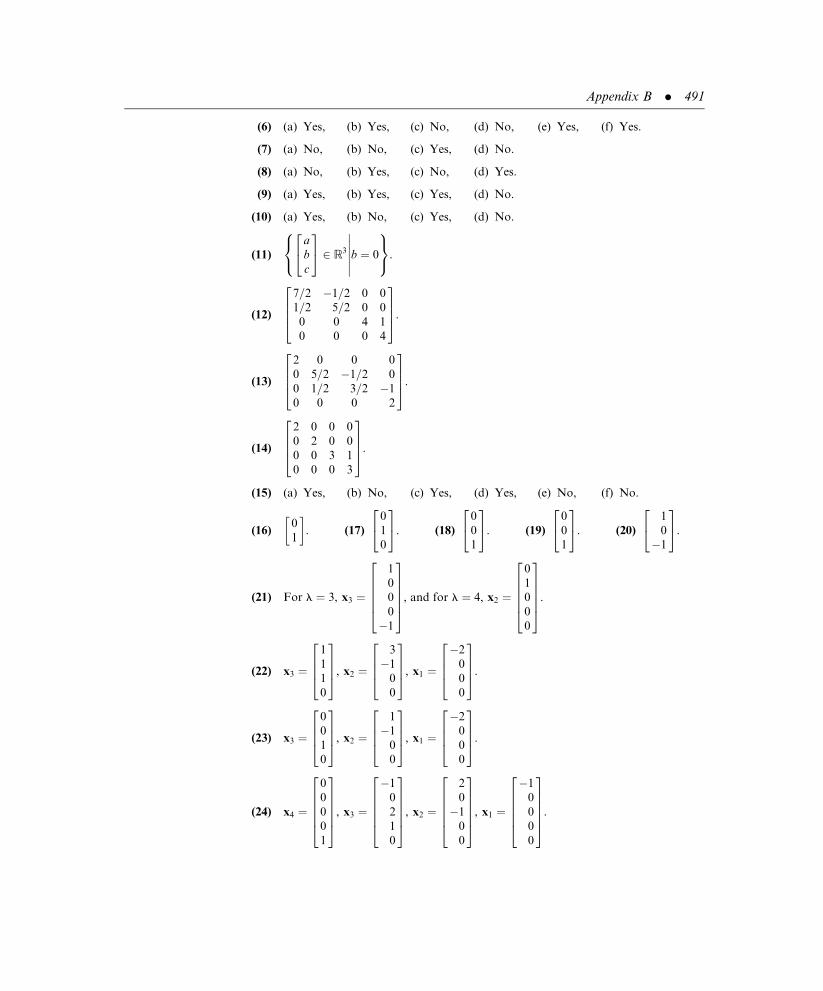
(6) (a) Yes, (b) Yes, (c) No, (d) No, (e) Yes, (f) Yes.
(7) (a) No, (b) No, (c) Yes, (d) No.
(8) (a) No, (b) Yes, (c) No, (d) Yes.
(9) (a) Yes, (b) Yes, (c) Yes, (d) No.
(10) (a) Yes, (b) No, (c) Yes, (d) No.
(11)
a
b
c
2435 2 R3
8<:
������b ¼ 0
9=;.
(12)
7=2 �1=2 0 0
1=2 5=2 0 0
0 0 4 1
0 0 0 4
2664
3775.
(13)
2 0 0 0
0 5=2 �1=2 0
0 1=2 3=2 �1
0 0 0 2
2664
3775.
(14)
2 0 0 0
0 2 0 0
0 0 3 1
0 0 0 3
2664
3775.
(15) (a) Yes, (b) No, (c) Yes, (d) Yes, (e) No, (f) No.
(16)0
1
� �. (17)
0
1
0
2435. (18)
0
0
1
2435. (19)
0
0
1
2435. (20)
1
0
�1
24
35.
(21) For l ¼ 3, x3 ¼
1
0
0
0
�1
266664
377775, and for l ¼ 4, x2 ¼
0
1
0
0
0
266664
377775.
(22) x3 ¼
1
1
1
0
26643775, x2 ¼
3
�1
0
0
2664
3775, x1 ¼
�2
0
0
0
2664
3775.
(23) x3 ¼
0
0
1
0
26643775, x2 ¼
1
�1
0
0
2664
3775, x1 ¼
�2
0
0
0
2664
3775.
(24) x4 ¼
0
0
0
0
1
266664
377775, x3 ¼
�1
0
2
1
0
266664
377775, x2 ¼
2
0
�1
0
0
266664
377775, x1 ¼
�1
0
0
0
0
266664
377775.
Appendix B . 491
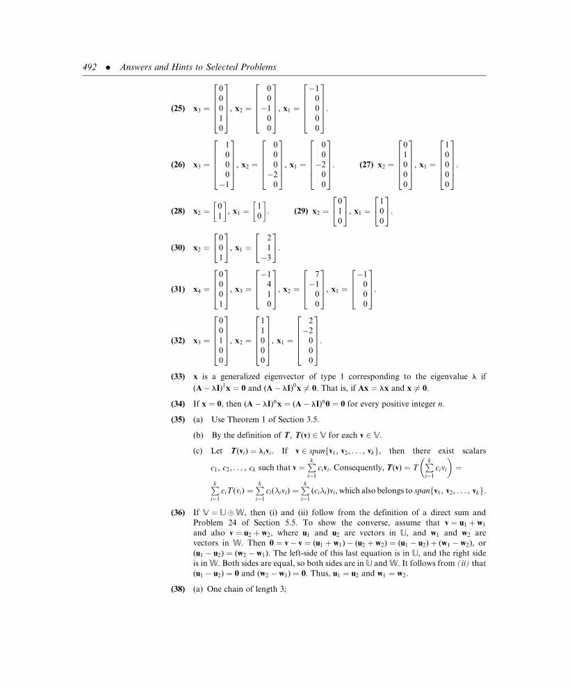
(25) x3 ¼
0
0
0
1
0
266664377775, x2 ¼
0
0
�1
0
0
266664
377775, x1 ¼
�1
0
0
0
0
266664
377775.
(26) x3 ¼
1
0
0
0
�1
266664
377775, x2 ¼
0
0
0
�2
0
266664
377775, x1 ¼
0
0
�2
0
0
266664
377775. (27) x2 ¼
0
1
0
0
0
266664
377775, x1 ¼
1
0
0
0
0
266664
377775.
(28) x2 ¼0
1
� �, x1 ¼
1
0
� �. (29) x2 ¼
0
1
0
2435, x1 ¼
1
0
0
2435.
(30) x2 ¼0
0
1
2435, x1 ¼
2
1
�3
24
35.
(31) x4 ¼
0
0
0
1
26643775, x3 ¼
�1
4
1
0
2664
3775, x2 ¼
7
�1
0
0
2664
3775, x1 ¼
�1
0
0
0
2664
3775.
(32) x3 ¼
0
0
1
0
0
266664377775, x2 ¼
1
1
0
0
0
266664377775, x1 ¼
2
�2
0
0
0
266664
377775.
(33) x is a generalized eigenvector of type 1 corresponding to the eigenvalue l if
(A� lI)1x ¼ 0 and (A� lI)0x 6¼ 0. That is, if Ax ¼ lx and x 6¼ 0.
(34) If x ¼ 0, then (A� lI)nx ¼ (A� lI)n0 ¼ 0 for every positive integer n.
(35) (a) Use Theorem 1 of Section 3.5.
(b) By the definition of T, T(v) 2 V for each v 2 V.
(c) Let T(vi) ¼ livi. If v 2 spanfv1, v2, . . . , vkg, then there exist scalars
c1, c2, . . . , ck such that v ¼Pki¼1
civi. Consequently, T(v) ¼ TPki¼1
civi
¼
Pki¼1
ciT(vi) ¼Pki¼1
ci(�ivi) ¼Pki¼1
(ci�i)vi, which also belongs to spanfv1, v2, . . . , vkg.
(36) If V ¼ U�W, then (i) and (ii) follow from the definition of a direct sum and
Problem 24 of Section 5.5. To show the converse, assume that v ¼ u1 þ w1
and also v ¼ u2 þ w2, where u1 and u2 are vectors in U, and w1 and w2 are
vectors in W. Then 0 ¼ v� v ¼ (u1 þ w1)� (u2 þ w2) ¼ (u1 � u2)þ (w1 � w2), or
(u1 � u2) ¼ (w2 � w1). The left-side of this last equation is in U, and the right side
is in W. Both sides are equal, so both sides are in U and W. It follows from (ii) that
(u1 � u2) ¼ 0 and (w2 � w1) ¼ 0. Thus, u1 ¼ u2 and w1 ¼ w2.
(38) (a) One chain of length 3;
492 . Answers and Hints to Selected Problems

(b) two chains of length 3;
(c) one chain of length 3, and one chain of length 2;
(d) one chain of length 3, one chain of length 2, and one chain of length 1;
(e) one chain of length 3 and two chains of length 1;
(f) cannot be done, the numbers as given are not compatible;
(g) two chains of length 2, and two chains of length 1;
(h) cannot be done, the numbers as given are not compatible;
(i) two chains of length 2 and one chain of length 1;
(j) two chains of length 2.
(39) x2 ¼0
1
� �, x1 ¼
1
�1
� �.
(40) x1 ¼�1
1
1
24
35 corresponds to l ¼ 1 and y2 ¼
0
0
1
2435, y1 ¼
3
0
�3
24
35 correspond to
l ¼ 4.
(41) x3 ¼0
0
1
2435, x2 ¼
�1
2
0
24
35, x1 ¼
2
0
0
2435.
(42) x1 ¼1
�2
0
24
35, y1 ¼
0
�2
1
24
35 both correspond to l ¼ 3 and z1 ¼
1
0
1
2435 corresponds
to l ¼ 7.
(43) x3 ¼
0
0
0
1
26643775, x2 ¼
�1
1
0
0
2664
3775, x1 ¼
1
0
0
0
26643775, y1 ¼
0
�1
1
�1
2664
3775.
(44) x2 ¼
0
1
0
0
26643775, x1 ¼
1
0
0
0
26643775 correspond to l ¼ 3 and y2 ¼
3
1
0
�1
2664
3775, y1 ¼
�1
�1
�1
0
2664
3775
correspond to l ¼ 4.
(45) x4 ¼
0
0
0
2
�2
1
26666664
37777775, x3 ¼
�1
1
2
0
0
0
26666664
37777775, x2 ¼
3
4
0
0
0
0
26666664
37777775, x1 ¼
4
0
0
0
0
0
26666664
37777775 correspond to l ¼ 4, and
y2 ¼
�5
�2
0
1
1
0
26666664
37777775, y1 ¼
3
2
1
1
0
0
26666664
37777775 correspond to l ¼ 5.
Appendix B . 493

(46)
2 0 0 0 0
0 2 0 0 0
0 0 2 1 0
0 0 0 2 1
0 0 0 0 2
266664
377775. (47)
2 1 0 0 0
0 2 0 0 0
0 0 2 1 0
0 0 0 2 1
0 0 0 0 2
266664
377775.
(48)
2 0 0 0 0
0 2 1 0 0
0 0 2 0 0
0 0 0 2 1
0 0 0 0 2
266664
377775. (49)
2 0 0 0 0
0 2 1 0 0
0 0 2 1 0
0 0 0 2 1
0 0 0 0 2
266664
377775.
(50)
2 1 0 0 0
0 2 1 0 0
0 0 2 1 0
0 0 0 2 1
0 0 0 0 2
266664
377775. (51)
3 1 0 0 0 0
0 3 1 0 0 0
0 0 3 0 0 0
0 0 0 3 1 0
0 0 0 0 3 1
0 0 0 0 0 3
26666664
37777775.
(52)
3 0 0 0 0 0
0 3 1 0 0 0
0 0 3 0 0 0
0 0 0 3 1 0
0 0 0 0 3 1
0 0 0 0 0 3
26666664
37777775. (53)
3 0 0 0 0 0
0 3 0 0 0 0
0 0 3 0 0 0
0 0 0 3 1 0
0 0 0 0 3 1
0 0 0 0 0 3
26666664
37777775.
(54)
3 1 0 0 0 0
0 3 0 0 0 0
0 0 3 1 0 0
0 0 0 3 0 0
0 0 0 0 3 1
0 0 0 0 0 3
26666664
37777775. (55)
3 0 0 0 0 0
0 3 0 0 0 0
0 0 3 1 0 0
0 0 0 3 0 0
0 0 0 0 3 1
0 0 0 0 0 3
26666664
37777775.
(56)
3 0 0 0 0 0
0 3 0 0 0 0
0 0 3 0 0 0
0 0 0 3 0 0
0 0 0 0 3 1
0 0 0 0 0 3
26666664
37777775.
(57) (a)
2 0 0 0
0 2 0 0
0 0 2 1
0 0 0 2
2664
3775, (b)
2 0 0 0
0 2 1 0
0 0 2 0
0 0 0 2
2664
3775,
(c)
2 1 0 0
0 2 0 0
0 0 2 0
0 0 0 2
2664
3775, (d)
2 1 0 0
0 2 0 0
0 0 2 0
0 0 0 2
2664
3775.
494 . Answers and Hints to Selected Problems
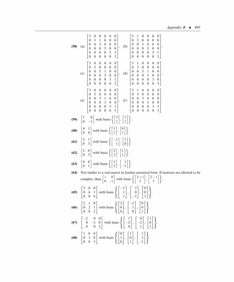
(58) (a)
3 0 0 0 0 0
0 3 1 0 0 0
0 0 3 0 0 0
0 0 0 5 0 0
0 0 0 0 5 1
0 0 0 0 0 5
26666664
37777775, (b)
3 1 0 0 0 0
0 3 0 0 0 0
0 0 3 0 0 0
0 0 0 5 0 0
0 0 0 0 5 1
0 0 0 0 0 5
26666664
37777775,
(c)
3 0 0 0 0 0
0 5 0 0 0 0
0 0 5 1 0 0
0 0 0 5 0 0
0 0 0 0 3 1
0 0 0 0 0 3
26666664
37777775, (d)
3 1 0 0 0 0
0 3 0 0 0 0
0 0 5 1 0 0
0 0 0 5 0 0
0 0 0 0 3 0
0 0 0 0 0 5
26666664
37777775,
(e)
3 0 0 0 0 0
0 5 0 0 0 0
0 0 3 1 0 0
0 0 0 3 0 0
0 0 0 0 5 1
0 0 0 0 0 5
26666664
37777775, (f )
5 1 0 0 0 0
0 5 0 0 0 0
0 0 5 0 0 0
0 0 0 3 0 0
0 0 0 0 3 1
0 0 0 0 0 3
26666664
37777775.
(59)1 0
0 �1
� �with basis
3
1
� �,
1
1
� �� �.
(60)4 1
0 4
� �with basis
1
1
� �,
0
1
� �� �.
(61)3 1
0 3
� �with basis
�1
1
� �,
1
0
� �� �.
(62)2 0
0 3
� �with basis
2
1
� �,
1
1
� �� �.
(63)4 0
0 1
� �with basis
1
2
� �,
1
�1
� �� �.
(64) Not similar to a real matrix in Jordan canonical form. If matrices are allowed to be
complex, theni 0
0 �i
� �with basis
2þ i
1
� �,
2� i
1
� �� �.
(65)
3 0 0
0 6 1
0 0 6
24
35 with basis
�1
1
1
24
35,
3
0
�3
24
35,
0
0
1
2435
8<:
9=;.
(66)
2 1 0
0 2 1
0 0 2
24
35 with basis
2
0
0
2435,
�2
1
0
24
35,
0
0
1
2435
8<:
9=;.
(67)
�2 0 0
0 �2 0
0 0 2
24
35 with basis
1
�2
0
24
35,
0
�2
1
24
35,
1
0
1
2435
8<:
9=;.
(68)
1 0 0
0 1 0
0 0 3
24
35 with basis
0
1
0
2435,
1
0
1
2435,
1
2
�1
24
35
8<:
9=;.
Appendix B . 495

(69)
0 0 0
0 2 1
0 0 2
24
35 with basis
5
�4
1
24
35,
�1
0
1
24
35,
1
0
0
2435
8<:
9=;.
(70)
0 0 0
0 0 0
0 0 14
24
35 with basis
3
0
�1
24
35,
�1
5
�3
24
35,
1
2
3
2435
8<:
9=;.
(71)
3 0 0 0
0 3 1 0
0 0 3 1
0 0 0 3
2664
3775 with basis
0
�1
1
�1
2664
3775,
1
0
0
0
26643775,
�1
1
0
0
2664
3775,
0
0
0
1
26643775
8>><>>:
9>>=>>;.
(72)
1 1 0 0
0 1 0 0
0 0 2 1
0 0 0 2
2664
3775 with basis
1
0
0
0
26643775,
0
1
0
0
26643775,
�1
�1
�1
0
2664
3775,
3
1
0
�1
2664
3775
8>><>>:
9>>=>>;.
(73)
1 0 0 0 0 0 0
0 1 0 0 0 0 0
0 0 1 1 0 0 0
0 0 0 1 1 0 0
0 0 0 0 1 0 0
0 0 0 0 0 1 1
0 0 0 0 0 0 1
2666666664
3777777775
with basis
0
0
�1
�2
1
0
0
2666666664
3777777775,
1
3
1
0
0
1
0
2666666664
3777777775,
�1
0
1
�1
0
0
0
2666666664
3777777775,
0
0
1
0
0
0
�1
2666666664
3777777775,
0
1
0
0
0
0
0
2666666664
3777777775,
�2
0
2
�2
0
0
�1
2666666664
3777777775,
1
0
0
0
0
0
0
2666666664
3777777775
8>>>>>>>><>>>>>>>>:
9>>>>>>>>=>>>>>>>>;
.
(74) If x is a generalized eigenvector of type m corresponding to the eigenvalue l, then
(A� lI)mx ¼ 0.
(75) Let u and v belong to Nl(A). Then there exist nonnegative integers m and n
such that (A� lI)mu ¼ 0 and (A� lI)nv ¼ 0. If n � m, then (A� lI)nu ¼(A� lI)n�m(A� lI)mu ¼ (A� lI)n�m0 ¼ 0. For any scalars a and b,
(A� lI)n(auþ bv) ¼ a[(A� lI)nu]þ b[(A� lI)nv] ¼ a0þ b0 ¼ 0. The reasoning
is similar if m > n.
(76) (A� lI)n is an nth degree polynomial in A, and A commutes with every polynomial
in A.
(77) If (A� lI)kx ¼ 0, then (A� lI)k(Ax) ¼ A[(A� lI)kx] ¼ A0 ¼ 0.
(78) If this was not so, then there exists a vector x 2 Rn such that (A� lI)k ¼ 0 and
(A� lI)k�1 6¼ 0 with k > n. Therefore, x is a generalized eigenvector of type k with
k > n. The chain propagated by x is a linearly independent set of k vectors in Rn
with k > n. This contradicts Theorem 3 of Section 2.4.
496 . Answers and Hints to Selected Problems

Appendix C(1) None of the matricies can be transition matrices. (a) Second column sum is greater
than unity. (b) Second column sum is less than unity. (c) Both column sums are
greater than unity. (d) Matrix contains a negative element. (e) Third column sum is
less than unity. (f) Third column sum is greater than unity. (g) None of the column
sums is unity. (h) Matrix contains negative elements.
(2)0:95 0:01
0:05 0:99
� �. (3)
0:6 0:70:4 0:3
� �.
(4)
0:10 0:20 0:25
0:50 0:60 0:65
0:40 0:20 0:10
24
35. (5)
0:80 0:10 0:25
0:15 0:88 0:30
0:05 0:02 0:45
24
35.
(6) (a) P2 ¼ 0:37 0:63
0:28 0:72
� �and P3 ¼ 0:289 0:316
0:711 0:684
� �,
(b) 0.37, (c) 0.63, (d) 0.711, (e) 0.684.
(7) 1! 1! 1! 1, 1! 1! 2! 1, 1! 2! 1! 1, 1! 2! 2! 1.
(8) (a) 0.097, (b) 0.0194.
(9) (a) 0.64, (b) 0.636.
(10) (a) 0.1, (b) 0.21.
(11) (a) 0.6675, (b) 0.577075, (c) 0.267.
(12) (a) There is a 0.6 probability that an individual chosen at random initially will live
in the city; thus, 60% of the population initially lives in the city, while 40% lives
in the suburbs.
(b) d(1) ¼ [ 0:574 0:426 ]T, (c) d(2) ¼ [ 0:54956 0:45044 ]T.
(13) (a) 40% of customers now use brand X, 50% use brand Y, and 10% use other
brands.
(b) d(1) ¼ [ 0:395 0:530 0:075 ]T, (c) d(2) ¼ [ 0:38775 0:54815 0:06410 ]T.
(14) (a) d(0) ¼ [ 0 1 ]T, (b) d(1) ¼ [ 0:7 0:3 ]T.
(15) (a) d(0) ¼ 0 1 0½ �T,
(b) d(3) ¼ [ 0:192 0:592 0:216 ]T. There is a probability of 0.216 that the harvest
will be good in three years.
(16) (a) [1=6 5=6]T, (b) 1=6.
(17) [ 7=11 4=11 ]T; probability of having a Republican is 7=11 � 0:636.
(18) [ 23=120 71=120 26=120 ]T; probability of a good harvest is 26=120 � 0:217.
(19) [ 40=111 65=111 6=111 ]T; probability of a person using brand Y is 65=111 ¼0:586.
Appendix C . 497

Appendix D(1) x ¼ 30 x model bicycles; y ¼ 20 y model bicycles; P¼ $410.
(2) x ¼ 35 x model bicycles; y ¼ 0 y model bicycles; P¼ $3500.
(3) x ¼ 120 x model bicycles; y ¼ 120 y model bicycles; P¼ $2640.
498 . Answers and Hints to Selected Problems

Index
A
Additive inverse, vectors in vector
space, 95–96
Angle between vectors, 297–299
Answers to selected problems,
431–498
Area, parallelogram, 358–362
Associativity
matrix addition, 5–6
matrix multiplication, 17
Augmented matrix
definition, 38
Gaussian elimination, 39–45
inverse, 53–56
simplex method, 426
B
Basis
change of, 187–199
eigenspace, 225–227
image of linear transformation,
206
kernel of linear transformation,
206
linear transformation, 178–183
orthogonal vector, 301–303
orthonormal basis, 312–313
row space, 138–141
vector space, 119–124, 138
Block diagonal matrix, 26–27, 381
C
Canonical basis
creation, 399–400
definition, 395
generalized eigenvector,
395–398
Cauchy-Schwartz Inequality, 300
Chain, see Markov chain; Vector
chain
Characteristic equation, 222
Closure under addition, 85–86
Closure under scalar multiplication,
85–86
Coefficient matrix, 12, 18, 57–58, 68
Cofactor, 355–357
Column index, 3
Column matrix, 3–4
Column rank, matrix, 145–147
Column space, 145
Commutativity, matrix addition, 5
Complex vector space, 86
Component, matrix, 3
Consistent system, simultaneous
linear equations, 35, 37,
148–149
Coordinate representation
basis change, 187–193
Euclidean inner product,
297–298
handedness, 77
vector, 126–127
Correspondence, rules of, 157–159
D
Dependence, linear, see Linear
dependence
Derivative, of a matrix, 256
Derived set, linear equations, 39–44
Determinant
calculation
cofactors, 355–357
diagonal matrix, 363
elementary row operations,
365–367
pivotal condensation, 368–370
rules based on minors, 354
triangular matrices, 362–363
definition, 353
invertible matrices, 370
parallelogram area, 358–362
similar matrices, 370
Diagonal element, matrix, 3
Diagonal matrix
definition, 26
derivative, 363
diagonalization, 219, 237–245
Differential equations
fundamental form
definition, 272
solution, 278–286
transformation, 273–275
matrix representation, 270–273
modeling, 288–290
software solutions, 429–430
Dilation, linear transformation, 164
499

Dimension
matrix, 4
n-space, 73
nullity and kernel dimension,
209
vector space, 124
Direct sum, 378, 381
Directed line segment, 75–76
Distribution vector, 416–417
Domain, 157–158, 163
Dominant eigenvalue, 259,
261–262
Duality, 427
E
Eigenspace
basis, 225–227
definition, 225
Eigenvalue
calculation for matrix, 222–225,
228–229
definition, 220
dominant eigenvalue, 259,
261–262
eigenvector pair, 221
exponential matrices, 255
geometric interpretation in
n-space, 220
inverse power method, 263–267
multiplicity, 224
properties, 232–235
QR algorithm for determination,
326–330
similar matrices, 224–225
Eigenvector
calculation for matrix, 222–225
definition, 220
diagonalization of matrices,
237–245
eigenvalue pair, 221
exponential matrices, 255
generalized, 395–398
geometric interpretation in
n-space, 220
properties, 232–235
type 2, 387
type 3, 384–385
Element, matrix, 2
Elementary matrix, 50–53
Elementary row operations
elementary matrix, 51–53
pivot, 40
simplex method, 425–427
Equations, simultaneous linear,
see Simultaneous linear
equations
Equivalent directed line segments,
75
Euclidean inner product, see also
Orthogonal complement
calculation, 295–296
definition, 295
geometrical interpretation,
297–298
induced inner product, 300–301,
310
Euler’s relations, 255
Expansion by cofactors, 356–357
Exponential matrix
calculation, 247–249
definition, 247
inverse, 253
Jordan canonical form, 249–252
F
Finite Markov chain, 413, 415, 418
Finite-dimensional vector space,
122, 124
Function, see also Transformation
definition, 157
notation, 159
rules of correspondence, 157–159
Fundamental form, differential
equations
definition, 272
solution, 278–286
transformation, 273–275
G
Gaussian elimination, simultaneous
linear equation solution,
38–44, 122, 149
Generalized eigenvector, 395–398
Generalized modal matrix, 402
Generalized Theorem of
Pythagoras, 299
Gram-Schmidt orthonormalization
process, 316–320
H
Homogeneous system
differential equations, 273
simultaneous linear equations,
36–37, 43, 50
I
Identity matrix, 26
Image, linear transformation,
204–209
Inconsistent system, simultaneous
linear equations, 35
Independence, linear, see Linear
independence
Index numbers, 393–394
Induced inner product, 300–301,
310
Infinite-dimensional vector space,
122
Initial conditions, 272–273
Initial tableau, 426
Initial-value problem, 273–276,
283
Inner product space, 314
Invariant subspace, 379–384, 388
Inverse
determinant of matrix, 370
exponential matrix, 253
matrix, 48–49, 51–59
Inverse power method, 263–267
J
Jordan block, 390–392
Jordan canonical form, matrix,
249–252, 390, 400–402
K
Kernel, linear transformation,
202–209
Kronecker delta, 310
500 . Index

L
Least-squares error, 333–334
Least-squares solution, 337–339
Least-squares straight line, 334
Left distributive law, matrix
multiplication, 17
Limiting state distribution vector,
419–420
Line segment, directed, 75–76
Linear combination, vectors
determination, 105–106
span, 106–107
Linear dependence
definition, 110
vector sets, 114–117, 123
Linear equations, see Simultaneous
linear equations
Linear independence
definition, 110
matrices, 112–113
polynomials, 142
row matrix, 150–151
row rank in determination,
141–142
three-dimensional row matrices,
111–112
two-dimensional row matrices, 111
vectors in a basis, 130
vector sets, 113–117
Linear transformation, see
Transformation
Lower triangular matrix, 27, 233, 362
LU decomposition, 63–69
M
MacLaurin series, 247
Magnitude
n-tuple, 296
row matrix, 73–75
vector, 296
Main diagonal, 3
Markov chain
definition, 413
distribution vector, 416
limiting state distribution vector,
419–420
transition matrix construction,
414
MATHEMATICA1, 429
MATLAB1, 429
Matrix, see also n-tuple
block diagonal matrix, 26–27
column matrix, 3–4
definition, 2
diagonal element, 3
diagonal matrix, 26
differential equation
representation, 270–273
elementary matrix, 50–52
elements, 2
Gaussian elimination for
simultaneous linear equation
solution, 38–44
identity matrix, 26
inverse, 48–49, 51–59
lower triangular matrix, 27
LU decomposition, 63–69
partitioned matrix, 24
row matrix, 3–4, 72
row space, 134–142
simplex method, 425–427
square matrix, 3
submatrix, 17
trace, 232
transpose of matrix, 22–24
upper triangular matrix, 27
zero row, 25–26
Matrix addition
associativity, 5–6
commutativity, 5
sum of matrices of same order, 5
Matrix multiplication
associativity, 17
coefficientmatrix, 12, 18, 57–58, 68
left distributive law, 17
packages approach, 12
postmultiplication, 14
premultiplication, 14
product of two matrices, 13–17
right distributive law, 17
scalar multiplication, 7–8
Matrix representation
change of basis, 195–199
linear transformation, 173–183,
194
Matrix subtraction, 6–7
Minimization, 427
Minor, matrix, 354
Modal matrix, 238–239, 248
Modeling, differential equations,
288–290
Multiplicity, eigenvalue, 224
N
Noise, 332
Nonhomogeneous system
differential equations, 273
simultaneous linear equations, 36
Nonsingular matrix, 49, 56–57
Normal equations, 335, 339
Normalization, n-tuples, 79
Normalized vector, 297
n-space
definition, 72
row space, see Row space
three-dimensional row matrices,
78–79
two-dimensional row matrices,
72–77
n-space
linear transformation, 176–179
subspace, 102–104
n-tuple
definition, 4
4-tuple, 79
5-tuple, 79
normalization, 79
sets, see n-space
three-dimensional row matrices,
78–79
two-dimensional row matrices,
72–77
Null space, linear transformation,
202
Nullity, kernel dimension, 209
O
Objective function, 425
One-to-one linear transformation,
210–213
Order, matrix, 2
Orthogonal complement
definition, 343
projection, 308–309
subspaces, 341–346
Orthogonal vector, 299, 301–303
Index . 501

Orthonormal basis, 312–313
Orthonormal set, 310–311, 315
Orthonormalization, Gram-
Schmidt orthonormalization
process, 316–320
P
Parallelogram, area, 358–362
Partitioned matrix, 24
Pivot
definition, 40
elementary matrix, 51–53
simplex method, 426
Pivotal condensation, 368–370
Postmultiplication, matrices, 14
Power method
calculation, 260–261
conditions, 259
inverse power method, 263–267
shifted inverse power method,
267–268
Premultiplication, matrices, 14
Problems, answers to, 431–498
Product, inner, see Inner product
Projection
onto x-axis, 168
onto x-axis, 169
orthogonal complement,
308–309
vector, 307–320
Pythagorean theorem, 299
Q
QR algorithm, 323–330, 429
QR decomposition, 323–325
R
Rn, see n-space
Range, 157–158, 163
Rank, 393–394, 397
Real number space, see n-space
Real vector space, 86
Reciprocal, see Inverse
Rectangular coordinate system,
handedness, 77
Reflection
across x-axis, 167
across y-axis, 168
Regular transition matrix,
418–419
Representation, matrix, see
Matrix representation
Residual, 333
Right distributive law, matrix
multiplication, 17
Row matrix, see also n-tuple
features, 3–4
linear independence, 150–151
three-dimensional row matrices,
78–79
two-dimensional row matrices,
72–77
Row rank
column rank relationship,
145–147
definition, 134
determination, 135–137
linear independence
determination, 141–142
Row-reduced matrix
Gaussian elimination, 39–45
transformation, 53
Row space
basis, 138–141
definition, 134
operations, 134–142
Rules of correspondence, 157–159
S
Scalar, see also Cofactor;
Determinant; Eigenvalue
definition, 7
linear equations, 33
Scalar multiplication
closure under scalar
multiplication, 85
matrix, 7–8
subspace, 100–102
vector space, 86, 92, 94–95
Scatter diagram, 331–332
Shifted inverse power method,
267–268
Similar matrices
definition, 199
determinants, 370
eigenvalues, 224–225
Simplex method, 425–427
Simultaneous linear equations
consistent system, 35, 37, 148–149
forms, 31–34
Gaussian elimination for
solution, 38–44
homogeneous system, 36–37, 43,
150
inconsistent system, 35
matrix representations, 32, 37
nonhomogeneous system, 36
trivial solution, 36
Singular matrix, 49, 233
Skew symmetric matrix, 24
Slack variables, 425–426
Span
basis, 138–139
row space of matrix, 134
subspace, 106–107, 119–120
vector chain, 388
Spectral matrix, 238–239
Square matrix, 3
Standard basis, 124–127
Submatrix, 17
Subspace
definition, 99
kernel of linear transformation,
202–204
n-space, 102–104
scalar multiplication, 100–102
span, 106–107, 119–120
vector space, 105–106
Superdiagonal, 390
Symmetric matrix, 24
T
Three-dimensional row matrices,
78–79
Trace, 232–233
Transformation, see also Function
change of basis, 187–199
definition, 163
diagonalization of matrices, 219,
237–245
dilation, 164
image, 202–209
kernel, 202–209
502 . Index

linear transformation
determinations, 164–170
properties, 201–213
matrix representation, 173–183
one-to-one transformation,
210–213
Transition matrix
change of basis, 188–194
construction for Markov chain,
414
definition, 413
powers of, 415–417
regular, 418–419
Transpose, of matrix, 22–24
Triangular matrix, see Lower
triangular matrix; Upper
triangular matrix
Two-dimensional row matrices,
72–77
U
Unit vector, 297
Upper triangular matrix, 27, 243,
362
V
Vector, see also Eigenvector; n-tuple
angle between vectors, 297–299
distribution vector, 416–417
least-squares solution, 337–339
limiting state distribution vector,
419–420
linear combination
determination, 105–106
span, 106–107
linear independence, 113–117,
130
magnitude, 296
orthogonal vector, 299, 301–303
orthonormal set, 310–311, 315
projection, 307–320
unit vector, 297
zero vector, 93–95
Vector chain, 386–388, 391
Vector multiplication, see Inner
product
Vector space
additive inverse of vectors, 95–96
basis, 119–124
closure under addition, 85–86
closure under scalar
multiplication, 85–86, 92
complex vector space, 86
definition, 86
dimension, 124
efficient characterization, 110
finite-dimensional vector space,
122, 124
infinite-dimensional vector space,
122
linear independence,
110–117
proof of properties, 87–93
real vector space, 86
row space of matrix, 134–142
set notation, 86–87
standard basis, 124–127
subspace, see Subspace
Z
Zero matrix, 377
Zero row, 25–26
Zero transformation, 165, 172
Zero vector, 93–95
Index . 503