Embed Size (px)
Citation preview
Line Fault Location in Emerging HVDC Transmission Systems
By Obada Mudalige Kasun Kavinda Nanayakkara
A thesis submitted to the Faculty of Graduate Studies
of the University of Manitoba
in partial fulfilment of the requirements for the degree of
Doctor of Philosophy
Department of Electrical and Computer Engineering University of Manitoba
Winnipeg, Manitoba, Canada
© Copyright 2014, Obada Mudalige Kasun Kavinda Nanayakkara

Abstract
The current technology used for location of permanent faults in high voltage direct cur-
rent (HVDC) transmission lines and cables is based on the travelling-wave principle. This
technology has served well for the conventional point-to-point HVDC systems, but is in-
adequate to handle emerging HVDC transmission configurations such as schemes with
very long overhead lines or cables, schemes with a combination of cables and overhead
line segments, and multi-terminal HVDC (MTHVDC) schemes. This research investi-
gated accurate and economical ways to locate the faults on dc transmission lines in the
aforementioned emerging HVDC transmission configurations.
The accuracy of travelling-wave based fault location methods is highly dependent on the
accuracy of measuring the time of arrival of the fault generated travelling waves. Investi-
gations showed that post-processing of detection signals such as the line terminal volt-
ages or surge capacitor currents with continuous wavelet transform yields consistent and
accurate fault location results. This method was applied for fault location in HVDC sys-
tems with extra-long overhead lines and cables using only the terminal measurements.
Simulation results verified the effectiveness of this method in locating the faults in a 2400
km long overhead line and a 300 km long underground cable.
i

A new algorithm was proposed to locate the faults in a two-terminal HVDC system con-
sisting of multiple segments of overhead lines and cables, using only the terminal meas-
urements. The application of the proposed algorithm was analysed through detailed simu-
lations. Correct performance was verified under various scenarios.
A new algorithm was developed for locating the faults in a star-connected MTHVDC
network. This algorithm also required only the terminal measurements. Its effectiveness
was verified through detailed simulations.
Finally, a novel measurement scheme for the detection of travelling-wave arrival times
was proposed. A prototype of this measurement scheme which uses a Rogowski coil to
measure the transient currents through the surge capacitors at the line terminals was im-
plemented. Its effectiveness was validated through field tests in a real HVDC transmis-
sion system. The proposed measurement scheme could capture significantly clean sig-
nals in an actual substation environment, confirming the practicability of implementing
the newly proposed algorithms.
ii

Acknowledgments
I would like to express my sincere thanks to Dr. Athula Rajapakse for his continuous
advice, guidance and encouragement throughout the course of this research. I consider
myself privileged to have had the opportunity to work under his guidance. I would also
like to thank Randy Wachal, Jean Sebestian and Warren Erickson at Manitoba Hydro In-
ternational for their support with providing resources, technical support and, feedback
throughout the research. The technical support received from the technical staff of the
University of Manitoba is highly appreciated. I also would like to extend my gratitude to
the Advisory Committee members for their comments and feedback to improve the qual-
ity of the thesis. The financial support received from the Natural Science and Engineering
Research Council, Manitoba Hydro, University of Manitoba Graduate Fellowship
(UMGF) and Manitoba Hydro International is gratefully acknowledged.
Special thanks to Gerald R. Brown and Yasas Rajapakse for the comments made to
improve my writing. Thanks to the staff and all of my colleagues in the Department of
Electrical and Computer Engineering for their continuous encouragement, and for mak-
ing my years at the University of Manitoba a pleasant experience. This acknowledgement
would not be complete without thanking my family. I extend my heartfelt gratitude to my
beloved parents, my wife and my brother.
O.M. Kasun Kavinda Nanayakkara
iii

Dedication
To mother, father, brother and wife.
iv
Contents
Front Matter Abstract ........................................................................................................... i
Contents ......................................................................................................... v
List of Tables .................................................................................................. x
List of Figures .............................................................................................. xii
List of Symbols .......................................................................................... xviii List of Abbreviations ................................................................................... xx
1 Introduction 1
1.1 Background ............................................................................................ 1
1.2 Motivation .............................................................................................. 3
1.3 Objectives ............................................................................................... 8
1.4 Thesis Overview..................................................................................... 8
2 Travelling-wave based fault-location in HVDC systems using wavelet transform 11
2.1 Introduction ......................................................................................... 11
2.2 Travelling-wave based fault-location .................................................. 12
2.3 Wavelet transform ............................................................................... 18
2.3.1 Discrete wavelet transform ...................................................... 20
2.4 Wavelet transform applications in power systems ............................ 21
v

3 DC line fault-location in HVDC systems with an extra-long dc line 23
3.1 Introduction ......................................................................................... 23
3.2 Test networks used for simulation studies ......................................... 24
3.2.1 HVDC test network with 2400 km long OH dc line ................ 27
3.2.2 HVDC test network with 300 km long UG cable dc line ......... 28
3.3 Wavelet based surge-arrival time detection ....................................... 29
3.3.1 Proposed fault-location algorithm ............................................ 30
3.3.2 Discrete Wavelet Transform (DWT) and Continuous Wavelet
Transform (CWT) ................................................................................. 31
3.3.3 Application to a sample waveform ........................................... 32
3.3.4 Effect of mother-wavelet type ................................................... 38
3.3.5 Effect of sampling frequency .................................................... 40
3.3.6 Determination of propagation velocity ..................................... 42
3.4 Simulation results for HVDC systems with extra-long dc line ......... 44
3.4.1 Simulation results: HVDC test network - 2400 km OH line .. 44
3.4.2 Simulation results: HVDC test network - 300 km UG cable .. 49
3.5 Effect of the noise in the input signal ................................................. 54
3.5.1 Performance with noisy inputs: HVDC test network with
2400 km long OH dc line ..................................................................... 55
3.5.2 Performance with noisy inputs: HVDC test network with 300 km long UG cable dc line .............................................................. 57
3.6 Concluding remarks ............................................................................ 59
4 Fault-location in conventional HVDC schemes with multiple segments 61
4.1 Introduction ......................................................................................... 61
4.2 Development of the fault-location algorithm for an HVDC transmission system with three line segments .......................................... 62
4.3 Identification of the faulty line segment ............................................ 64
4.4 Calibration of the system .................................................................... 66
4.5 Identification of the fault arrival time ................................................ 67
vi
4.6 Simulated case study ........................................................................... 68
4.6.1 Monitored signals ...................................................................... 69
4.6.2 Identification: Faulty-line segment using simulation results. 70
4.6.3 Fault-location results ................................................................ 71
4.7 Fault-location with noisy inputs ......................................................... 73
4.8 Fault-location performance for high impedance faults ...................... 76
4.9 Theoretical extension of the algorithm to an 'n'-segment HVDC transmission system .................................................................................... 77
4.10 Concluding remarks ............................................................................ 79
5 Fault-location in star-connected multi-terminal HVDC schemes 81
5.1 Introduction ......................................................................................... 81
5.2 Development of the algorithm for fault-location method in star connected three terminal HVDC transmission system .............................. 83
5.3 Identification: Correct faulty dc line ................................................... 87
5.4 Calibration of the system .................................................................... 90
5.5 Identification of the fault arrival time ................................................ 91
5.6 Simulated case study ........................................................................... 93
5.6.1 Simulation model ...................................................................... 93
5.6.2 Simulation results ..................................................................... 95
5.6.3 Identification of the faulty line segment using the simulation results ................................................................................................... 97
5.7 Theoretical extension of the algorithm to star-connected network with n-number of terminals ........................................................................ 98
5.8 Concluding remarks .......................................................................... 102
6 Implementation and field validation of a travelling-wave arrival-time measurement scheme 103
6.1 Introduction ....................................................................................... 103
6.2 Arrangement of the surge-arrival time measurement system ........ 105
vii

6.3 Rogowski coil ...................................................................................... 106
6.4 Layout of the prototype measurement unit ...................................... 108
6.4.1 Specifications of the Rogowski coil ......................................... 109
6.4.2 Surge protection unit and trigger pulse generating circuit .. 113
6.4.3 Data acquisition hardware ..................................................... 115
6.4.4 Specifications: GPS (Global Positioning System) .................. 116
6.4.5 Specifications: Personal computer and the wireless communication module ...................................................................... 117
6.4.6 Software for capturing waveforms ......................................... 119
6.4.7 Rogowski coil placement at the converter station ................. 120
6.5 Summary of the recorded events ...................................................... 122
6.5.1 Lightning strike caused event ................................................ 126
6.5.2 Identification of a disturbance occurred in pole 3 ................. 127
6.6 Simulation study ............................................................................... 128
6.6.1 Test network ........................................................................... 129
6.6.2 Rogowski coil simulation model ............................................. 130
6.6.3 Simulation results ................................................................... 131
6.6.4 Rogowski coil and ‘Haar’ wavelet transform ......................... 134
6.6.5 Fault-location results .............................................................. 135
6.7 Concluding remarks .......................................................................... 136
7 Conclusions and contributions 138
7.1 Conclusions ........................................................................................ 138
7.2 Contributions ..................................................................................... 141
7.3 Suggestions for future research ........................................................ 143
Appendix A: Wavelet Transform 145
A.1 Introduction ....................................................................................... 145
A.2 Haar wavelet ...................................................................................... 146
A.3 Example calculation of Haar wavelet coefficients ............................ 149
viii

Appendix B: Steps to set up GPS unit 151
B.1 Enable TIM-TM2 messages in the UART port ................................. 151
B.2 Configuration of the GPS unit's UART port data transmitting protocol settings ......................................................................................... 152
B.3 Enable TIM-TM2 type messages in the GPS unit ............................ 152
B.4 Location calibration of the GPS unit ................................................ 153
References 155
ix

List of Tables
Table 3-1 - Calibrated propagation constant values for OH line HVDC test network ..... 43
Table 3-2 - Calibrated propagation constant values for UG cable HVDC test network ... 43
Table 3-3 - Fault-location results with different CWT coefficients (scales 4, 8, 16, and
32) of the terminal voltages .............................................................................................. 45
Table 3-4 - Fault-location results with different CWT coefficients (scale 4, 8, 16, and 32)
of the surge capacitor currents .......................................................................................... 46
Table 3-5 - Fault-location results with different DWT coefficients (levels 2, 3, 4, and 5)
of the terminal voltages ..................................................................................................... 47
Table 3-6 - Fault-location results with different DWT coefficients (levels 2, 3, 4, and 5)
of the surge capacitor currents .......................................................................................... 48
Table 3-7 - Fault-location results with different CWT coefficients (scales 4, 8, 16, and
32) of the terminal voltages .............................................................................................. 50
Table 3-8 - Fault-location results with different CWT coefficients (scales 4, 8, 16, and
32) of the surge capacitor currents .................................................................................... 51
Table 3-9 - Fault-location results with different DWT coefficients (levels 2, 3, 4, and 5)
of the terminal voltages ..................................................................................................... 52
Table 3-10 - Fault-location results with different DWT coefficients (levels 2, 3, 4, and 5)
of the surge capacitor currents .......................................................................................... 53
x

Table 3-11 - Comparison of fault-location errors with different CWT scales of the
terminal voltages with 0.001 pu noise .............................................................................. 59
Table 4-1 - Calculated values of xF1, xF2, and xF3 for different fault locations ................. 71
Table 4-2 - Predicted fault-location and estimation errors with terminal voltage ............ 72
Table 4-3 - Predicted fault-location and estimation errors with surge capacitor current .. 72
Table 4-4 - Predicted fault-location and estimation errors with terminal voltage
contaminated with 0.001 pu noise .................................................................................... 74
Table 4-5 - Predicted fault-location and estimation errors with terminal voltage
contaminated with 0.01 pu noise ...................................................................................... 74
Table 4-6 - Predicted fault-location and estimation errors with surge capacitor current
contaminated with 0.001 kA noise.................................................................................... 75
Table 4-7 - Predicted fault-location and estimation errors with surge capacitor current
contaminated with 0.01 kA noise...................................................................................... 75
Table 4-8 - Predicted fault-location and estimation errors for high impedance faults using
scale-32 CWT coefficients ................................................................................................ 76
Table 5-1 - Calculated values of xT1, xT2 , RT and XF for different fault locations ............ 96
Table 6-1 - Self and mutual inductance values of different Rogowski coils .................. 112
Table 6-2 - Serial communication pin assignment ......................................................... 117
Table 6-3 - Comparison of fault-location & surge-arrival time difference of event 1 ... 123
Table 6-4 - Comparison of fault-location & surge-arrival time difference of event 10 . 126
Table 6-5 - Comparison of fault locations ...................................................................... 136
Table A-1 – Example of calculated Haar wavelet coefficients ....................................... 149
xi

List of Figures
Fig. 2-1 - Bewley lattice diagram for a fault at (a) first half of the line (at A) and (b)
second half of the line (at B) ............................................................................................. 14
Fig. 2-2 - Different types of wavelets ............................................................................... 20
Fig. 2-3 - Structure of one-level DWT algorithm ............................................................. 21
Fig. 3-1 - HVDC test networks modeled in PSCAD/EMTDC ......................................... 26
Fig. 3-2 - HVDC dc line parameters (Left: OH line tower structure and Right: UG cable
parameters) ........................................................................................................................ 27
Fig. 3-3 - Comparisons of original terminal voltages and surge capacitor currents with
conditioned signals when permanent dc line fault occurred at 100 km from the rectifier
end ..................................................................................................................................... 28
Fig. 3-4 - Comparisons of original terminal voltages and surge capacitor currents with
conditioned signals when permanent dc line fault occurred at 175 km from the rectifier
end (300 km UG cable HVDC test network) .................................................................... 29
Fig. 3-5 - Simplified WT based LFL algorithm ................................................................ 31
Fig. 3-6 - Terminal voltages and surge capacitor currents when permanent dc line fault
occurred at (a) 625 km (b) 100 km (c) 2100 km from the rectifier end ............................ 33
xii
Fig. 3-7 - DWT and CWT coefficient magnitude values of rectifier end voltage and surge
capacitor current when a line to ground fault occurred (625 km away from the rectifier
end applied at 2.4 s) .......................................................................................................... 35
Fig. 3-8- DWT and CWT coefficient magnitude values of rectifier end voltage and surge
capacitor current when a line to ground fault occurred (2100 km away from the rectifier
end applied at 2.4 s) .......................................................................................................... 37
Fig. 3-9 - DWT and CWT coefficient magnitude values of rectifier end voltage and surge
capacitor current when a line to ground fault occurred (100 km away from the rectifier
end applied at 2.4 s) .......................................................................................................... 38
Fig. 3-10 - Comparison coefficient magnitudes of different mother wavelets ................. 39
Fig. 3-11 - Effect of sampling frequency .......................................................................... 41
Fig. 3-12 - Fault-location errors with different CWT coefficients (scale 4, 8, 16, and 32)
of the terminal voltages ..................................................................................................... 45
Fig. 3-13 - Fault-location errors with different CWT coefficients (scales 4, 8, 16, and 32)
of the surge capacitor currents .......................................................................................... 46
Fig. 3-14 - Fault-location errors with different DWT coefficients (levels 2, 3, 4, and 5) of
the terminal voltages ......................................................................................................... 48
Fig. 3-15 - Fault-location errors with different DWT coefficients (levels 2, 3, 4, and 5) of
the surge capacitor currents .............................................................................................. 49
Fig. 3-16 - Fault-location errors with different CWT coefficients (scales 4, 8, 16, and 32)
of the terminal voltage ...................................................................................................... 50
Fig. 3-17 - Fault-location errors with different CWT coefficients (scales 4, 8, 16, and 32)
of the surge capacitor currents .......................................................................................... 51
xiii

Fig. 3-18 - Fault-location results with different DWT coefficients (levels 2, 3, 4, and 5) of
the terminal voltages ......................................................................................................... 53
Fig. 3-19 - Fault-location results with different DWT coefficients (levels 2, 3, 4, and 5) of
the surge capacitor currents .............................................................................................. 54
Fig. 3-20 - Surge capacitor current and terminal voltage with added noise ..................... 55
Fig. 3-21 - Prediction errors for different noise levels in the terminal voltages (Using
CWT Scale 4) .................................................................................................................... 56
Fig. 3-22 - Prediction errors for different noise levels in the surge capacitor current
measurements (Using CWT Scale 4) ................................................................................ 56
Fig. 3-23 - Comparison of prediction errors using different CWT scales for terminal
voltage with 0.005pu of noise ........................................................................................... 57
Fig. 3-24 - Prediction errors for different noise levels in the terminal voltages (Using
CWT Scale 16) .................................................................................................................. 58
Fig. 3-25 - Prediction errors for different noise levels in the surge capacitor current
measurements (Using CWT Scale 16) .............................................................................. 58
Fig. 4-1 - HVDC system with two segments of OH lines and one segment of cable ....... 62
Fig. 4-2 - Three-segment test network .............................................................................. 68
Fig. 4-3 - Monitored input signals conditioned by A/D for a fault occurred 16 km away
from rectifier terminal ....................................................................................................... 70
Fig. 4-4 - Surge capacitor current and terminal voltage with added white noise ............. 73
Fig. 4-5 - HVDC system with “n” number of line segments where fault is in ith segment77
Fig. 5-1 - (a) Star connected three-terminal HVDC system (b) dc line fault F1 inside line
AD ..................................................................................................................................... 84
xiv
Fig. 5-2 - (a) dc line fault F2 inside the BD line (b) dc line fault F3 inside the CD line ... 86
Fig. 5-3 - Faulty segment identification and fault calculation method ............................. 89
Fig. 5-4 - Surge detection system for VSC HVDC systems (Redrawn from [46]) .......... 92
Fig. 5-5 - (a) Test network topology & line length (b) Measured terminal dc line current
........................................................................................................................................... 93
Fig. 5-6 - Tower structure for OH line segments .............................................................. 94
Fig. 5-7 - (a) Monitored dc line current signals conditioned by A/D, (b) Zoomed view of
the signals, and (c) the corresponding Scale-32 CWT coefficients for a fault occurred in
line BD, 10 km away from B terminal .............................................................................. 96
Fig. 5-8 - N-terminal VSC HVDC system with all dc lines connect to a common point . 98
Fig. 5-9 - Faulty segment identification and fault calculation method for network with 'N'
terminals .......................................................................................................................... 101
Fig. 6-1 - Wave-front detection system .......................................................................... 105
Fig. 6-2 - Flexible Rogowski coil ................................................................................... 106
Fig. 6-3 - Layout of the experimental setup at one converter station ............................. 108
Fig. 6-4 - Technical details of the selected Rogowski coil (Redrawn from [56] ) ......... 109
Fig. 6-5 - Test network modeled in PSCAD/EMTDC .................................................... 110
Fig. 6-6 - Surge capacitor current after applying a fault 1 km from rectifier (a) complete
view of the two end surge capacitor currents (b) zoomed in view to show the inverter end
surge capacitor current .................................................................................................... 110
Fig. 6-7 - Comparison of Rogowski coil output voltages (a) Complete view (b) Zoomed
in view to clearly show the first slope ............................................................................ 112
Fig. 6-8 - Installed Rogowski coil at Dorsey converter station ...................................... 113
xv

Fig. 6-9 – (a) Surge-protection and (b) trigger-pulse generating circuits as appear in the
experimental unit ............................................................................................................ 113
Fig. 6-10 - Multifunction Data Acquisition hardware NI USB-6361 from National
Instruments ...................................................................................................................... 115
Fig. 6-11 - Pin layout of NI USB 6361 ........................................................................... 115
Fig. 6-12 - GPS unit: EVK-6T-0 u-blox 6 Evaluation Kit with Precision Timing ......... 116
Fig. 6-13 - Front and real panels of the GPS unit ........................................................... 116
Fig. 6-14 - IPn3G - 3G Cellular Ethernet/Serial/USB Gateway ..................................... 117
Fig. 6-15 - ARK-3360F Embedded Box PC from AdvanTech ...................................... 118
Fig. 6-16 - Simplified flow diagram of the developed software ..................................... 119
Fig. 6-17 - Map of the Nelson River HVDC Transmission System with installed locations
of the fault locators ......................................................................................................... 121
Fig. 6-18 - Placement of the experimental unit in Nelson River HVDC line (Under
normal operation of Nelson River system) ..................................................................... 121
Fig. 6-19 - Venn diagram view of recorded events ........................................................ 122
Fig. 6-20 - Histogram view of the fault-location from Dorsey in Kilometers ................ 122
Fig. 6-21 - Captured waveform from the experimental unit (First recorded event) ....... 123
Fig. 6-22 - Colour map view of captured Rogowski coil voltages in volts .................... 124
Fig. 6-23 - Captured Rogowski coil pre fault voltages for selected events .................... 125
Fig. 6-24 - Captured voltages for event 10 ..................................................................... 126
Fig. 6-25 - Fault-location on the map obtained with Manitoba Hydro's lightning strike
locator ............................................................................................................................. 127
Fig. 6-26 - Nelson River HVDC system dc tower operation under normal condition ... 127
xvi
Fig. 6-27 - Event 3 occurred on pole 3 ........................................................................... 128
Fig. 6-28 - Simulation model .......................................................................................... 130
Fig. 6-29 - Equivalent circuit of the Rogowski coil........................................................ 130
Fig. 6-30 - Surge capacitor currents after dc line fault occurred 1 km from the rectifier
end. In the second graph y-axis is expanded to show the details of inverter side waveform
......................................................................................................................................... 132
Fig. 6-31 - CWT coefficient magnitudes and Rogowski coil voltage magnitude obtained
from surge capacitor currents at the terminals for ground fault occurred on the dc line 1
km from the rectifier station. .......................................................................................... 133
Fig. 6-32 - Frequency response of the Rogowski coil .................................................... 135
Fig. A-1 - Haar wavelet and its shifting process ............................................................. 147
Fig. A-2 - Haar wavelets at different scales .................................................................... 148
Fig. A-3 – Comparison of Haar wavelet and its scale 32 version with an example surge
capacitor current signal ................................................................................................... 148
Fig. A-4 – Input signal used in example calculation ...................................................... 150
Fig. A-5 – Calculated Haar detail coefficients at 3 levels .............................................. 150
Fig. B-1 - Configure GPS message protocol .................................................................. 151
Fig. B-2 - Configure port protocol settings ..................................................................... 152
Fig. B-3 - Enable TIM-TM2 messages ........................................................................... 153
Fig. B-4- GPS survey-in ................................................................................................. 154
xvii

List of Symbols
X Fault location
L Total dc line length
T1 Inverter terminal surge-arrival time
T2 Rectifier terminal surge-arrival time
V or v Travelling-wave propagation velocity
td1 Time difference: Arrival of first and the second surges at the first side
td2 Time difference: Arrivals of the initial surges at two sides of the line
f(t) Input signal
ψ(t) Mother wavelet
a Scaling factor
b Shifting factor
n Any integer value
k Sample number
td Difference between the initial surge-arrival times at the two terminals
λ Inverse of propagation velocity
R Ratio between the smaller and the larger values of the estimated fault locations
V0 Induced terminal voltage output of Rogowski coil
μ0 Permeability of free space (4π×10−7 H·m−1)
xviii

A Area of one loop of Rogowski coil
N Number of helical turns in Rogowski coil
l Length of the winding of the Rogowski coil
ML Mutual inductance
SL Self inductance
Zl Load resistance
SR Coil resistance
Cl Coil capacitance
f Frequency
j Unit imaginary number
xix

List of Abbreviations
ac Alternating Current
A/D Analog to Digital Conversion
AI Analog Input
ANN Antenna
COM Serial Communication Port
CWT Continuous Wavelet Transform
DAQ Data Acquisition Hardware
dc Direct Current
DI Digital Input
DSP Digital Signal Processor
DWT Discrete Wavelet Transform
EMT Electromagnetic Transient
EMTP Electromagnetic Transient Program
FORX Fibre Optic Receiver
FOTX Fibre Optic Transmitter
FPGA Field-programmable Gate Array
GND Ground
GPS Global Positioning System
xx

GSM Global System for Mobile
HPF High Pass Filter
HVDC High Voltage Direct Current
IEEE Institute of Electrical and Electronics Engineers
IGBT Insulated Gate Bipolar Transistor
LCC Line Commutated Converter
LFL Line Fault Locator
LPF Low Pass Filter
MTHVDC Multi-terminal High Voltage Direct Current
MTS Manitoba Telecom Services Inc
NI National Instruments Corporation
NMEA National Marine Electronics Association
OH Overhead
PC Personal Computer
PSCAD Power System Computer Aided Design
SIM Subscriber Identity Module
TTL Transistor–Transistor Logic
UART Universal Asynchronous Receiver/Transmitter
UBX U-blox GPS Communication Protocol
UG Underground
UHVDC Ultra High Voltage Direct Current
USB Universal Serial Bus
UTC Coordinated Universal Time
xxi

VSC Voltage Source Converter
WT Wavelet Transform
xxii
Chapter 1
Introduction
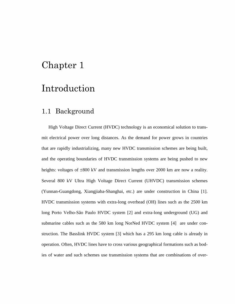
1.1 Background
High Voltage Direct Current (HVDC) technology is an economical solution to trans-
mit electrical power over long distances. As the demand for power grows in countries
that are rapidly industrializing, many new HVDC transmission schemes are being built,
and the operating boundaries of HVDC transmission systems are being pushed to new
heights: voltages of ±800 kV and transmission lengths over 2000 km are now a reality.
Several 800 kV Ultra High Voltage Direct Current (UHVDC) transmission schemes
(Yunnan-Guangdong, Xiangjiaba-Shanghai, etc.) are under construction in China [1].
HVDC transmission systems with extra-long overhead (OH) lines such as the 2500 km
long Porto Velho-São Paulo HVDC system [2] and extra-long underground (UG) and
submarine cables such as the 580 km long NorNed HVDC system [4] are under con-
struction. The Basslink HVDC system [3] which has a 295 km long cable is already in
operation. Often, HVDC lines have to cross various geographical formations such as bod-
ies of water and such schemes use transmission systems that are combinations of over-
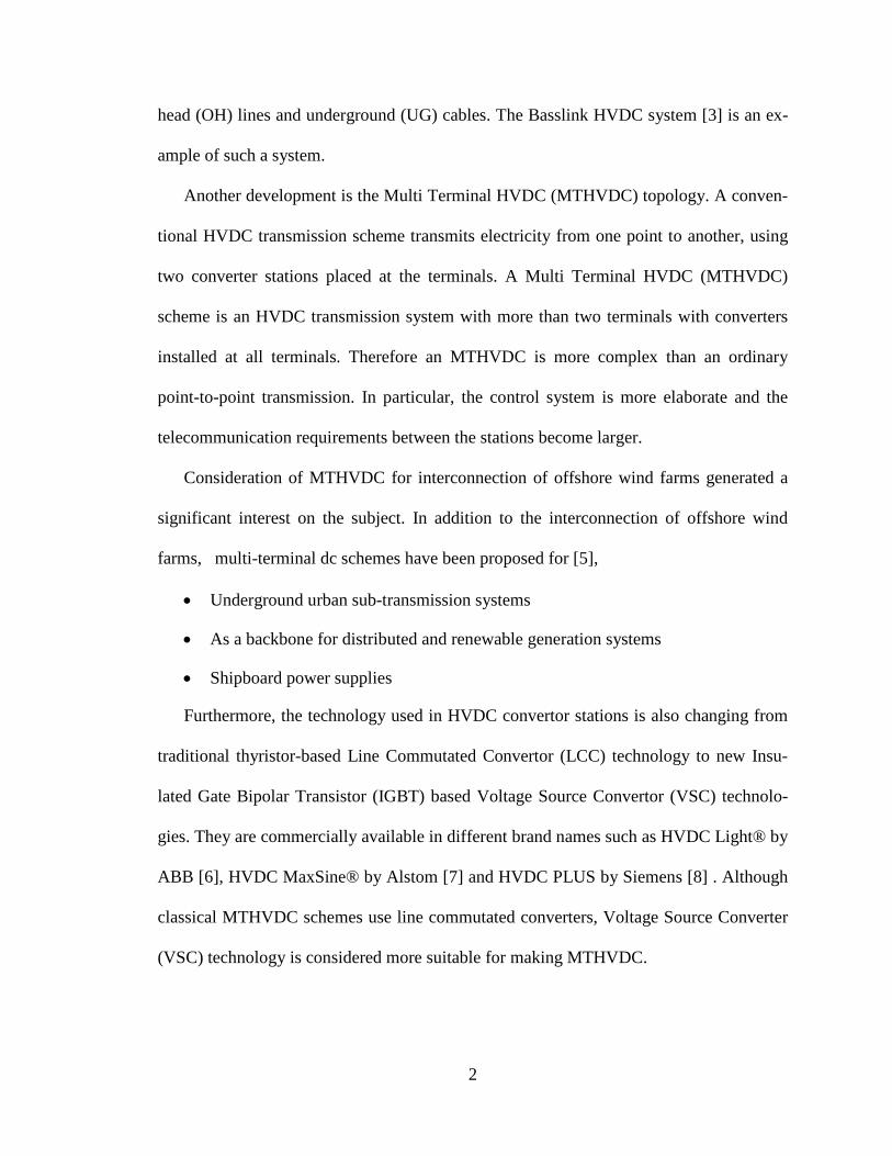
head (OH) lines and underground (UG) cables. The Basslink HVDC system [3] is an ex-
ample of such a system.
Another development is the Multi Terminal HVDC (MTHVDC) topology. A conven-
tional HVDC transmission scheme transmits electricity from one point to another, using
two converter stations placed at the terminals. A Multi Terminal HVDC (MTHVDC)
scheme is an HVDC transmission system with more than two terminals with converters
installed at all terminals. Therefore an MTHVDC is more complex than an ordinary
point-to-point transmission. In particular, the control system is more elaborate and the
telecommunication requirements between the stations become larger.
Consideration of MTHVDC for interconnection of offshore wind farms generated a
significant interest on the subject. In addition to the interconnection of offshore wind
farms, multi-terminal dc schemes have been proposed for [5],
• Underground urban sub-transmission systems
• As a backbone for distributed and renewable generation systems
• Shipboard power supplies
Furthermore, the technology used in HVDC convertor stations is also changing from
traditional thyristor-based Line Commutated Convertor (LCC) technology to new Insu-
lated Gate Bipolar Transistor (IGBT) based Voltage Source Convertor (VSC) technolo-
gies. They are commercially available in different brand names such as HVDC Light® by
ABB [6], HVDC MaxSine® by Alstom [7] and HVDC PLUS by Siemens [8] . Although
classical MTHVDC schemes use line commutated converters, Voltage Source Converter
(VSC) technology is considered more suitable for making MTHVDC.
2

1.2 Motivation
According to reliability statistics of HVDC systems during 2009-2010 found in [9], it
is clear that a certain percentage of forced energy outages occur due to transmission line
or cable related disturbances. Minimizing the outage time is critical both in terms of reli-
ability and loss of revenues, since HVDC systems are used to transport large amounts of
power. Furthermore, unavailability of an HVDC transmission system can impose limita-
tions on the operation of the rest of the system. Therefore, fault-location is of paramount
importance once a permanent fault occurs in an HVDC transmission line.
When a temporary fault occurs, the HVDC line protection system detects and extin-
guishes the fault by means of control actions as mentioned in [10] and [11], so that the
system can be restored as fast as possible. However, in case of permanent faults, the sys-
tem may need to terminate the power transmission until the necessary repairs are per-
formed on the line. Broadly two types of dc lines: overhead lines and cables are used in
HVDC systems. The causes for dc line faults can be due to electrical failures and me-
chanical failures. Mechanical failures are typical in submarine (underwater) cables and
are caused by a trawler anchor hooked to the cable or the fishing nets [12]. In overhead
line systems, failures are mostly due to flashovers and rarely due to tower collapses. The
most common cause for permanent damage to insulators in an overhead line is a lightning
surge that is high enough to cause a line flashover. Occasionally, flashover is caused by
normal voltage on account of the excessive contamination due to pollution and damaged
insulations. As regards to the dc line fault type, line-to-ground faults are the most fre-
quent in an HVDC system due to the tower structure, and pole-to-pole faults are rare
since typically the right of way is wider compared to the ac counterpart.
3

Location of a fault, as accurately as possible, is important to send the repair crews to
the right point on the HVDC line. The most fundamental way of fault location is by foot
patrols or by patrols equipped with different transportation means and vision aids. Such
means of inspections are considered time consuming and not feasible in HVDC systems
with long overhead lines or underground/submarine cable systems. Automatic fault loca-
tors are used to pinpoint the fault position by processing the voltage and/or current wave-
form values. The calculations required for the fault location can be performed in off-line
mode since the results of the calculations are for the operator’s use. This implies that the
speed of fault location calculations can be measured in seconds or even minutes [13].
This type of fault location can be classified into the following main categories:
1. Techniques based on resistance calculation performed using voltage and current
measurements.
2. Knowledge-based approaches.
3. Techniques based on injection of current signals.
4. Techniques based on travelling-wave phenomenon.
Impedance based methods (e.g. [14] and [15]) typically require line parameters, and
the voltage and current measurements during the fault. Reference [14], presents an im-
pedance based method which used post fault voltage and current data together with dc
line parameters to locate faults. In this method, the distributed parameter line model is
used and hence the voltage distribution over the line is obtained from the voltage and cur-
rent measurements at the two terminals. Using the voltage distribution, the fault point is
identified. These methods typically require a lower signal sampling rate than in the trav-
elling-wave based methods, and therefore can be implemented using data from the exist-
ing transient fault recorders at the converter stations. However these methods have a
4
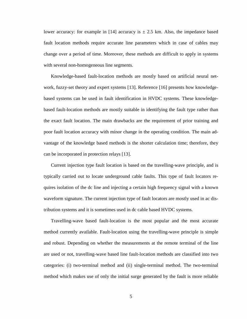
lower accuracy: for example in [14] accuracy is ± 2.5 km. Also, the impedance based
fault location methods require accurate line parameters which in case of cables may
change over a period of time. Moreover, these methods are difficult to apply in systems
with several non-homogeneous line segments.
Knowledge-based fault-location methods are mostly based on artificial neural net-
work, fuzzy-set theory and expert systems [13]. Reference [16] presents how knowledge-
based systems can be used in fault identification in HVDC systems. These knowledge-
based fault-location methods are mostly suitable in identifying the fault type rather than
the exact fault location. The main drawbacks are the requirement of prior training and
poor fault location accuracy with minor change in the operating condition. The main ad-
vantage of the knowledge based methods is the shorter calculation time; therefore, they
can be incorporated in protection relays [13].
Current injection type fault location is based on the travelling-wave principle, and is
typically carried out to locate underground cable faults. This type of fault locators re-
quires isolation of the dc line and injecting a certain high frequency signal with a known
waveform signature. The current injection type of fault locators are mostly used in ac dis-
tribution systems and it is sometimes used in dc cable based HVDC systems.
Travelling-wave based fault-location is the most popular and the most accurate
method currently available. Fault-location using the travelling-wave principle is simple
and robust. Depending on whether the measurements at the remote terminal of the line
are used or not, travelling-wave based line fault-location methods are classified into two
categories: (i) two-terminal method and (ii) single-terminal method. The two-terminal
method which makes use of only the initial surge generated by the fault is more reliable
5

than the single-terminal method which requires the use of secondary reflections. If the
two-terminal measurements are fully synchronized, the difference between the surge-
arrival times at the two terminals can be used to determine the fault-location, given that
the propagation velocity of the surge is known. With the development of Global Position-
ing System (GPS) which facilitates accurate time synchronization of the measurements at
the two terminals, the two-terminal method has become the most widely used technique.
The main disadvantages of the two-terminal methods are the requirements for high sam-
pling frequency transducers capable of capturing travelling waves and the very accurate
time synchronization of measurements. More details on this method are discussed in
Chapter 2.
HVDC transmission systems with extra-long OH lines (e.g. 2500 km long Porto
Velho-São Paulo HVDC system [2]) and HVDC systems with extra-long UG cables (e.g.
295 km long Basslink HVDC system [3] ) are under consideration. Accurate fault loca-
tion in such extra-long dc lines is a challenging task. Fault-location in extra-long HVDC
systems is currently achieved with the help of repeater stations. Installation of extra
hardware at the repeater stations, which are required to locate line faults using the exist-
ing technology, increases the cost of these transmission projects.
Due to high demand in HVDC systems, dc lines have to cross various geographical
areas. Therefore, OH lines combined with UG cables become an intricate part of the
HVDC system (e.g. [17] and [18]). Existing travelling-wave-based dc line fault-location
methods have been developed for the HVDC systems with only overhead transmission
lines. Fault-location in HVDC systems with a combination of overhead lines and cables
has been generally achieved by considering the overhead sections only. However, this
6

practice is expensive as it requires duplicate installation of additional hardware for each
overhead section.
Multi-terminal voltage-source converter (VSC) based HVDC technology is now
commercially available and expected to be widely used for the interconnection of off-
shore wind farms, as well as in underground urban sub-transmission systems, shipboard
power supplies and on shore renewable generation systems [5]. If a line fault occurs in a
multi-terminal HVDC scheme, the primary protection must activate and isolate the
faulted line segment. Some methods to identify the faulty line in a multi-terminal VSC
HVDC network with mesh topology are explained in [5] and [19]. These methods based
on current and voltage measurements at the converter terminals have been primarily de-
veloped for protection purposes. However, in the case of a permanent dc line fault, as
mentioned above, determination of the exact fault-location is essential for carrying out
the repairs. This can be achieved by using the existing two-terminal travelling-wave
based fault locators with synchronized measurements, if fault locators are placed at all the
terminals and at the common point. However, installing a fault locator at every connec-
tion point requires additional equipment as well as communication infrastructure, and
therefore incurs additional costs.
On the grounds of aforementioned reasons, this thesis focuses on elaborating on the
problems associated with fault-location in HVDC systems with extra-long dc lines, with
several non-homogeneous segments of dc lines and star-connected networks, and pro-
vides new exclusive algorithms and field validation data.
7
1.3 Objectives
The overall goal of this research is to improve the accuracy of travelling-wave based
fault-location technology for HVDC transmission systems, extend the applicability of
technology for emerging new HVDC topologies, and field validate a transducer to cap-
ture the travelling waves. The following specific objectives were fulfilled to achieve the
overall goal:
1. Development of improved methods to detect travelling waves and measure the
travelling-wave arrival times
2. Identification of suitable input signals which can be used to determine the travel-
ling-wave arrival times and the required signal conditioning needs
3. Development of fault-location algorithms that are suitable for the following
HVDC transmission system configurations:
I. Classical two-terminal HVDC schemes with very long (> 2000 km) OH
lines
II. Classical two-terminal HVDC schemes with very long (> 300 km) UG
cables
III. Classical two-terminal HVDC schemes with segments of OH lines and
UG cables
IV. VSC based star connected multi-terminal HVDC schemes
4. Identification of the hardware specifications for implementation of the fault loca-
tor in a classical HVDC system.
1.4 Thesis Overview
The thesis covers five areas: (1) review of the existing travelling-wave based fault-
location technology used in HVDC systems, (2) the author’s contributions on dc line
fault-location in extra-long HVDC lines and cables, (3) HVDC systems with several dc
8
line segments, and (4) multi-terminal HVDC systems, and (5) hardware implementation
details. This chapter provides an introduction giving the background information with the
problem statement and the research objectives.
A background to the travelling-wave based fault-location concept is provided in
Chapter 2. A brief introduction to the wavelet transform is given and some example ap-
plications of the wavelet transform in the power system field is presented. Then a wavelet
transform based surge detection method is explained. The effects of the sampling fre-
quency and mother wavelet type are discussed.
In Chapter 3, fault-location in a 2400 km long overhead HVDC line and a 300 km
long underground HVDC cable using the two-terminal travelling-wave method are inves-
tigated. The relative merits of using the terminal voltage and the terminal surge capacitor
current for the detection of travelling waves are examined. Practical considerations such
as the influences of noise, A/D conversion precision and the fault impedance on the fault-
location accuracy were also investigated.
In Chapter 4, a novel method is proposed for locating faults in an HVDC system with
a combination of overhead lines and cables by using only the terminal measurements.
The method can determine the faulted line segment and the exact fault-location.
Chapter 5 presents a new fault-location method for locating faults in star-connected
Multi terminal HVDC systems. The method can find the faulty line segment and calculate
the distance to the fault from a terminal using only the surge-arrival times measured at
the terminal.
Details about the implementation of an experimental line fault locator are presented in
Chapter 6. The proposed hardware specifications and measurement transducer usage are
9

validated by installing experimental data acquisition units at the Nelson River HVDC
system. Disturbances that occurred during July to September 2012 were monitored and
analysed in detail.
Finally in Chapter 7, conclusions and a summary of the contributions are presented.
10
Chapter 2
Travelling-wave based fault-location
in HVDC systems using wavelet transform
2.1 Introduction
The travelling-wave based fault-location principle, which utilizes the propagation
times of the voltage and current travelling waves generated on a transmission line when a
fault occurs, is well known. Although direct application of this principle is challenging in
the highly branched and meshed ac networks, it has been successfully applied to trans-
mission line fault-location in the conventional HVDC systems [20] - [28], which have
only two terminals. The key requirement to improve the accuracy of fault-location in long
lines is precise detection of the wave-front arrival times.
In many of the recently published research [26]-[28], surge-arrival times have been
detected using the Discrete Wavelet Transform (DWT) coefficients of the measured sig-
nals. Wavelet transform works well for analyzing transients in signals because of its si-
multaneous time and frequency localization capabilities. Availability of software tools
11

and a lower computational burden have made the discrete version of the wavelet trans-
form, DWT, the common choice for implementation of these fault-location algorithms.
Compared to DWT, continuous-wavelet transform (CWT) provides more a detailed
and continuous analysis of a fault transient [29]. In CWT, the analyzing wavelet is shifted
smoothly along the time axis of the input signal. Therefore, CWT coefficients have better
time resolution, which is very important to have high accuracy in travelling-wave based
dc line fault-location.
This chapter introduces the Travelling-wave based fault-location concept, and Wave-
let transform and its applications. It also explains mathematical details of the Discrete
Wavelet Transform (DWT) and Continuous Wavelet Transform (CWT).
2.2 Travelling-wave based fault-location
Travelling-wave based fault-location can be applied to both ac and dc transmission
lines. The flashover at the fault point launches two waves that travel in opposite direc-
tions away from the fault. If the transients appearing at either end of the line are captured,
they can be analysed to determine the fault position. HVDC transmission lines are ideal
for the application of travelling-wave theory as they are mainly used for point to point
transmission.
There are two types of fault-location algorithms differentiated according to the num-
ber of measurement locations used: (i) two-ended method and (ii) one-ended method.
Travelling-wave based fault-location in ac transmission lines is clearly described in IEEE
standard C37.114-2004 [30]. However, there is no such standard for fault-location in dc
transmission lines.
12
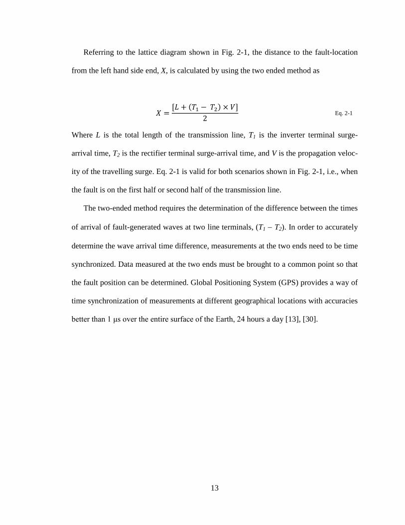
Referring to the lattice diagram shown in Fig. 2-1, the distance to the fault-location
from the left hand side end, X, is calculated by using the two ended method as
𝑋 =[𝐿 + (𝑇1 − 𝑇2) × 𝑉]
2 Eq. 2-1
Where L is the total length of the transmission line, T1 is the inverter terminal surge-
arrival time, T2 is the rectifier terminal surge-arrival time, and V is the propagation veloc-
ity of the travelling surge. Eq. 2-1 is valid for both scenarios shown in Fig. 2-1, i.e., when
the fault is on the first half or second half of the transmission line.
The two-ended method requires the determination of the difference between the times
of arrival of fault-generated waves at two line terminals, (T1 − T2). In order to accurately
determine the wave arrival time difference, measurements at the two ends need to be time
synchronized. Data measured at the two ends must be brought to a common point so that
the fault position can be determined. Global Positioning System (GPS) provides a way of
time synchronization of measurements at different geographical locations with accuracies
better than 1 μs over the entire surface of the Earth, 24 hours a day [13], [30].
13

T2
T1
3T1
X Y
A
T1
T2
YX
B
T1+2T2
(a) (b)
Fig. 2-1 - Bewley lattice diagram for a fault at (a) first half of the line (at A) and (b) second half of the line (at B)
The travelling-wave propagation velocity V is a parameter in Eq. 2-1 and the value of
V can change from scheme to scheme and with aging, especially in cables. If secondary
reflections are used, the travelling velocity of the signal can be excluded from the evalua-
tion process given that the fault is permanent and an accurate surge-arrival time detection
method is available. In order to eliminate the travelling-wave velocity from the calcula-
tions, the time between the arrival of the first and the second surges must be measured.
The first surge starts at the inception of the fault whereas the second surge corresponds to
the reflection at the remote end or fault point. If the fault occurs between the fault locator
and the midpoint of the protected line, the first reflection from the fault point arrives at
the fault locator before any other reflection from the remote end as shown in Fig. 2-1 (a).
On the other hand, if the fault occurs between the midpoint and remote end bus, reflec-
14
tions from the remote end may arrive at the fault locator before the first reflection from
the fault point, as shown in Fig. 2-1(b).
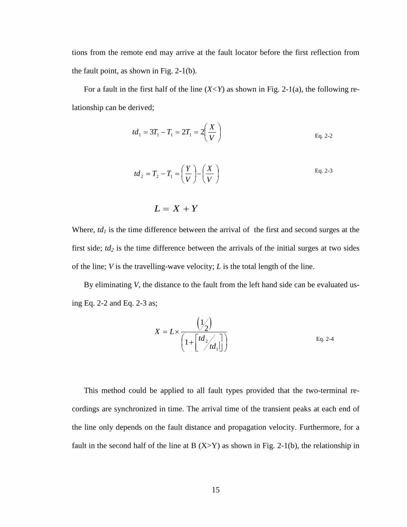
For a fault in the first half of the line (X<Y) as shown in Fig. 2-1(a), the following re-
lationship can be derived;
==−=
VXTTTtd 223 1111
Eq. 2-2
−
=−=
VX
VYTTtd 122 Eq. 2-3
YXL +=
Where, td1 is the time difference between the arrival of the first and second surges at the
first side; td2 is the time difference between the arrivals of the initial surges at two sides
of the line; V is the travelling-wave velocity; L is the total length of the line.
By eliminating V, the distance to the fault from the left hand side can be evaluated us-
ing Eq. 2-2 and Eq. 2-3 as;
( )
+
×=
1
21
21
tdtd
LX
Eq. 2-4
This method could be applied to all fault types provided that the two-terminal re-
cordings are synchronized in time. The arrival time of the transient peaks at each end of
the line only depends on the fault distance and propagation velocity. Furthermore, for a
fault in the second half of the line at B (X>Y) as shown in Fig. 2-1(b), the relationship in
15

Eq. 2-7 can be derived. Eq. 2-4 and Eq. 2-7, which are independent of the velocity of
propagation, can be used to calculate the fault distance X
==−+=VYTTTTtd 22)2( 11211
Eq. 2-5
−
=−=
VY
VXTTtd 212
Eq. 2-6
+
+
×=
1
2
1
2
1
21
tdtd
tdtd
LX
Eq. 2-7
On the other hand, the single-ended method does not require remote end synchroni-
zation. It makes use of fault induced spikes and one reflected surge to determine the fault-
location. However, in this case, due to the lack of any other time reference, all time
measurements will be with respect to the instant when the fault generated transient is first
detected. For a fault in the first half of the line (X<Y) as shown in Fig. 2-1(a);
==−=
VXTTTtd 223 1111
12tdVX ×= Eq. 2-8
For a fault in the second half of the line (X>Y) as shown in Fig. 2-1(b);
==−+=VYTTTTtd 22)2( 11211
XLY −=
16

12tdVLX ×−= Eq. 2-9
Eq. 2-8 and Eq. 2-9 can be used to calculate the fault distance X. In this case both
equations are dependent of the velocity of propagation. The one-ended principle is more
cost effective to be realized, but its reliability is not satisfactory due to the complexity of
fault reflected surge discrimination. The two-ended principle is more reliable than the
one-ended method as it only makes use of the initial fault generated surges.
The following equipment is necessary to locate faults using the two-terminal travel-
ling-wave method [30]:
1. Accurate time stamping device (GPS) on both ends of the line.
2. An appropriate sensor to detect the voltage travelling-waves or current travelling-
waves, depending on the parameter used.
3. A communications circuit is required to transmit the time stamped data back to a
central location.
4. A computer capable of retrieving the remote time stamp data or extracting wave
front arrival times from the appropriate waveforms, and performing the required
calculations to determine the fault-location using Eq. 2-1.
The accuracy of travelling-wave based fault-location directly depends on the accuracy
of measuring the relevant surge-arrival time differences. Since the velocity of propaga-
tion of travelling waves in transmission lines is close to the speed of light, an error of one
micro-second in the time difference measurement translates into approximately 300 m er-
ror in the fault-location. Detection of the precise arrival times of the wave fronts is very
important. Transducer bandwidths and signal sampling rates are thus a concern in practi-
cal implementation. If using the one ended measurements, distinguishing between travel-
ling waves reflected from the fault and from the remote end of the line is a problem [30].
17

However, the developments in transducer technology and broad bandwidth sampling ca-
pability have eased some of the practical difficulties of travelling-wave based methods
for fault-location. Furthermore, modern signal processing techniques such as wavelet
transform have shown to be useful in locating the transients such as travelling-wave
fronts superimposed on signals.
2.3 Wavelet transform
The wavelet transform is a linear transformation similar to the Fourier transform.
However, it is different from the Fourier transform because it allows the time localization
of different frequency components of a given signal [31].
The continuous wavelet transform (CWT) of a signal f(t) is the integral of the product
between f(t) and the daughter-wavelets, which are time translated and scale expanded or
compressed versions of a function ψ(t), which is called the mother-wavelet. Therefore,
CWT of a signal f(t) with respect to the mother wavelet ψ(t) is written as
𝐶𝑊𝑇(𝑓(𝑡);𝑎, 𝑏) = 𝑓(𝑡)𝜓∗𝑎,𝑏(𝑡)𝑑𝑡
∞
−∞ Eq. 2-10
𝜓∗𝑎,𝑏(𝑡) =
1√𝑎
𝜓 𝑡 − 𝑏𝑎
Eq. 2-11
Where Ψa, b (t) is a continuous function in both the time domain and the frequency do-
main called the mother-wavelet which is defined by Eq. 2-11 and * represents operation
of complex conjugate. “a” is a scaling factor and “b” is the shifting factor.
18
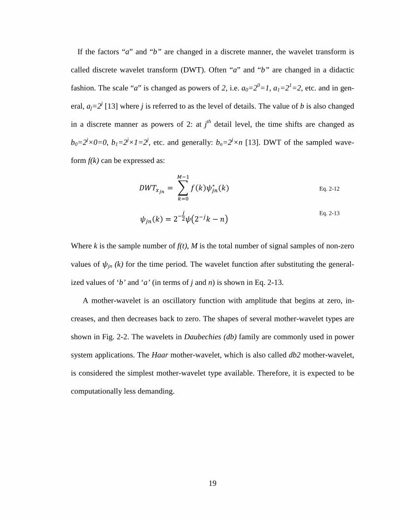
If the factors “a” and “b” are changed in a discrete manner, the wavelet transform is
called discrete wavelet transform (DWT). Often “a” and “b” are changed in a didactic
fashion. The scale “a” is changed as powers of 2, i.e. a0=20=1, a1=21=2, etc. and in gen-
eral, aj=2j [13] where j is referred to as the level of details. The value of b is also changed
in a discrete manner as powers of 2: at jth detail level, the time shifts are changed as
b0=2j×0=0, b1=2j×1=2j, etc. and generally: bn=2j×n [13]. DWT of the sampled wave-
form f(k) can be expressed as:
𝐷𝑊𝑇𝑥𝑗𝑛 = 𝑓(𝑘)𝜓𝑗𝑛∗ (𝑘)𝑀−1
𝑘=0
Eq. 2-12
𝜓𝑗𝑛(𝑘) = 2−𝑗2𝜓2−𝑗𝑘 − 𝑛
Eq. 2-13
Where k is the sample number of f(t), M is the total number of signal samples of non-zero
values of 𝜓jn (k) for the time period. The wavelet function after substituting the general-
ized values of ‘b’ and ‘a’ (in terms of j and n) is shown in Eq. 2-13.
A mother-wavelet is an oscillatory function with amplitude that begins at zero, in-
creases, and then decreases back to zero. The shapes of several mother-wavelet types are
shown in Fig. 2-2. The wavelets in Daubechies (db) family are commonly used in power
system applications. The Haar mother-wavelet, which is also called db2 mother-wavelet,
is considered the simplest mother-wavelet type available. Therefore, it is expected to be
computationally less demanding.
19

Fig. 2-2 - Different types of wavelets
2.3.1 Discrete wavelet transform
Discrete wavelet transform (DWT) has been used to detect incoming travelling waves
in many fault-location algorithms [26], [27], [28]. This has probably been motivated by
the computational efficiency of DWT over its continuous version. The DWT, which is
also considered as multi-resolution analysis, differs from continuous wavelet transform
(CWT) with clear steps in the time-frequency plane [22]. The DWT can be used to de-
compose the input signal into multiple frequency bands and this can be implemented effi-
ciently as a filter bank as shown in Fig. 2-3 under DWT decomposition [22]. Only a sin-
gle level is shown in Fig. 2-3 but this can be extended for a series of levels by substitut-
ing the approximation value with the input signal of the next level.
Meyer Wavelet
Morlet wavelet Mexican Hat wavelet
Haar wavelet
20

X(n)
HPF
LPF
↓2
↓2
Xd(n)
Xa(n)
Detail
Approximation
DWT decomposition
X(n)
HPF1
LPF1
↑2
↑2
Xd(n)
Xa(n)
Detail
Approximation
DWT reconstruction
Fig. 2-3 - Structure of one-level DWT algorithm
This implementation is commonly known as Mallat tree algorithm and consists of a
series of low-pass filters (LPF) and their dual high pass filters (HPF). The circle with a
downward arrow behind 2 denotes down sampling by a factor of 2. The output xd(n) is
called the detail wavelet coefficients while the output from the last low pass filter is re-
ferred to as the approximation wavelet coefficient.
It is possible to obtain the original signal x(t) through wavelet series reconstruction.
The reconstruction can also be carried out efficiently using a tree algorithm as shown in
Fig. 2-3 under DWT reconstruction. The filters HPF1 and LPF1 are the inverse filters of
HPF and LPF respectively. In Fig. 2-3, the circles with an upward arrow behind 2 de-
notes up sampling by a factor of 2.
2.4 Wavelet transform applications in power
systems
Wavelet analysis is widely used in image processing, medical imaging, communica-
tion and acoustics [24]. Wavelet transform is suited for the analysis of signals containing
21
short-lived high frequency disturbances superposed on lower frequency continuous wave-
forms [31]. Thus, in power systems, wavelet analysis is used for the detection of signal
features such as transients in the identification of power quality disturbances. The multi-
resolution properties of wavelet transform are useful for analyzing fault transients that
contain localized high frequency components superposed on power frequency signals
[31].
The wavelet transform can be used for detecting travelling waves in the line fault-
location. As mentioned earlier, in travelling-wave based fault-location systems, accurate
detection of the travelling-wave arrival time is very important. Wavelet coefficients of
the recorded voltage and current signals can be used to recognize the arrival of wave
fronts at the measuring point. Usually the discrete wavelet transform is applied to the de-
tection signal yielding the wavelet coefficients in selected levels. The correct fault posi-
tion will be determined by analyzing the relationship between the characteristics of the
transient sequences. Each transient signal is identified with a synchronizing time at its lo-
cal maximum value. The first local maximum represents the arrival of the initial wave
generated by the fault; the second local maximum represents the arrival of the first re-
flected wave and so on.
22
Chapter 3
DC line fault-location in HVDC
systems with an extra-long dc line
3.1 Introduction
With the rapid development of HVDC technology, HVDC transmission systems with
extra-long overhead (OH) lines or underground (UG) cables are coming into existence.
The 2500 km long Porto Velho-São Paulo HVDC system [2] and the 295 km long
Basslink HVDC system [3] are good examples. Accurate fault-location in such extra-long
HVDC transmission lines or cables is a challenging task because the travelling waves get
attenuated along the line.
Fault-location in such extra-long HVDC systems is currently achieved by sectioning
the line into two or more segments and installing repeater stations [21] at segment
boundaries. Installation of extra fault-location hardware at the repeater stations increases
the cost of these transmission projects.
This chapter investigates the possibility of accurately locating the faults on such ex-
tra-long OH lines and UG cables only using terminal measurements. It explores how the
wavelet coefficients of the measured signals, obtained using the DWT and CWT dis-
23
cussed in the previous chapter, can be used to more accurately detect the travelling wave
arriving times at the terminals. All studies were carried out with detailed models of
HVDC converters, transmission lines and cables simulated in PSCAD/EMTDC. The
fault-location algorithm was implemented in MATLAB. The importance of calibrating
the travelling-wave speed is highlighted as the travelling waves have different velocities
at different frequencies. Therefore propagation velocities are calibrated to each of the
scale of the wavelet coefficients used. Furthermore, the accuracy of the fault-location of
the proposed method was studied under noisy input signals.
3.2 Test networks used for simulation studies
Simulations were done using two HVDC transmission networks, one with an OH
transmission line and the other with a UG cable. Travelling wave propagation velocities
are different in OH lines and UG cables. OH lines are built with bare conductors (typi-
cally aluminum) mounted on towers which can be made from wood, steel, or concrete.
Electricity can be also be transmitted through cables running underground or undersea
(submarine). UG cables typically have the conductor covered with insulating materials
(e.g. oil, paper, XLPE), armour and a sheath cover. Travelling-wave travels at a higher
speed in OH lines (close to the speed of light) than in UG cables (approximately half of
the speed of light). The propagation velocity is a function of line parameters. In a loss
less line, it is equal to 1 √𝐿 ∙ 𝐶⁄ where L is the line inductance per unit length and C is the
line capacitance per unit length [13]. Because of the construction of UG cables, they
typically have higher per unit capacitances compared to OH lines. Therefore they have
24
lower propagation velocity. Attenuation is another issue that is important in travelling-
wave based fault-location. Attenuation coefficient of a transmission line is proportional to
the square root of line impedance and admittance per unit length [13]. Attenuation of
travelling waves is faster in UG cables compared to OH line due to dielectric losses in the
cable insulation. These dielectric losses substantially increase with the frequency. There-
fore it is important to analyse the proposed fault location method in those two types of dc
lines.
Both test networks are modified versions of the first Cigré benchmark HVDC scheme
[32]. This test network has 500 kV as the nominal dc voltage and it is designed to deliver
1000 MW of active power. Furthermore, a bipolar HVDC configuration is used since
most of the present day HVDC systems are built in a bipolar configuration, instead of the
mono-polar arrangement in the original reference.
The simplified lumped parameter “π” - model that represents a cable HVDC line
scheme in the original Cigré model [32] was replaced with a frequency-dependent dis-
tributed-parameter model of a 2400 km long overhead transmission line in the OH line
based test network. In the other test network based on UG cable, the simplified π - model
was replaced with a frequency dependent distributed parameter model of a 300 km long
underground cable. The schematic diagram of the test networks is shown in Fig. 3-1.
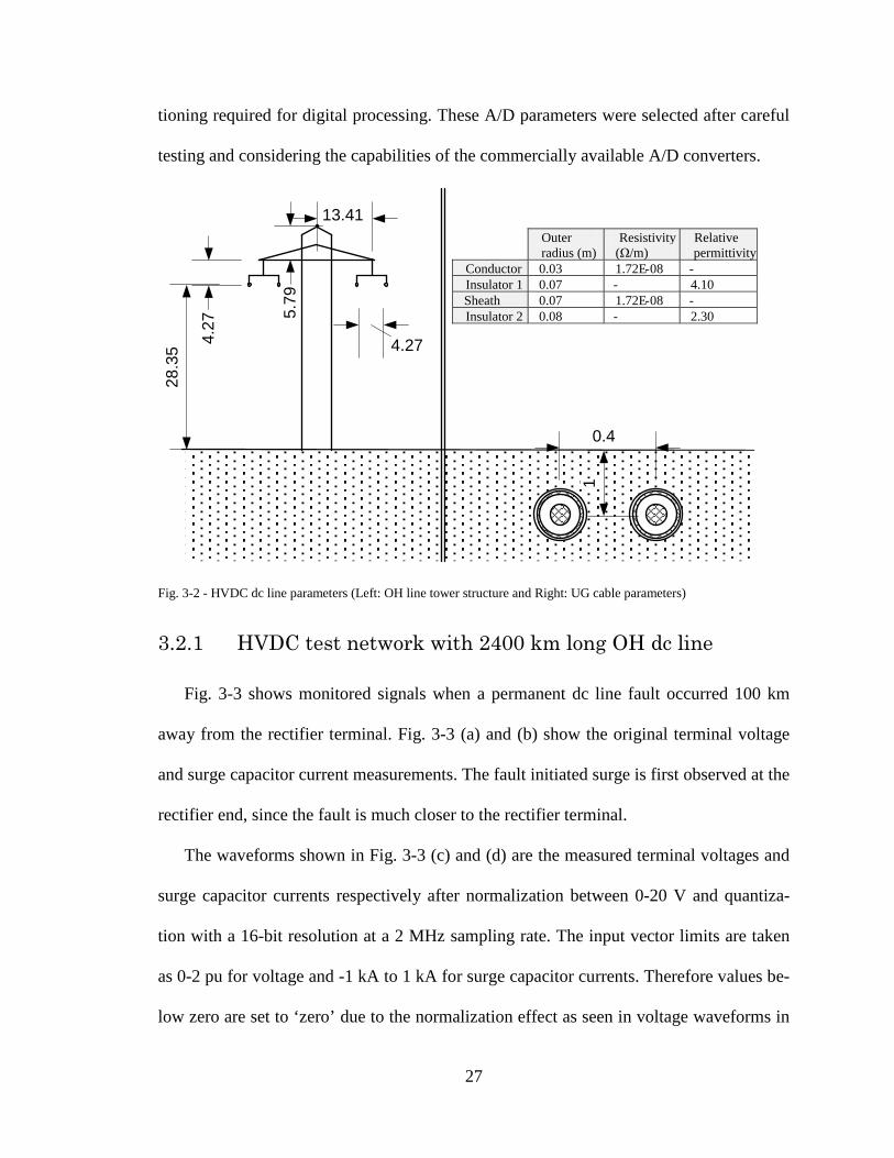
The tower structure for the OH dc line and cable parameters for the UG dc line are
shown in Fig. 3-2. All the distance measurements are shown in metres. The original test
network does not contain a surge capacitor. A surge capacitor is used to protect the con-
verter station equipment from surges travelling along the dc line. The steep wave-front of
a surge travelling along the dc transmission line is first attenuated by the line surge im-
25
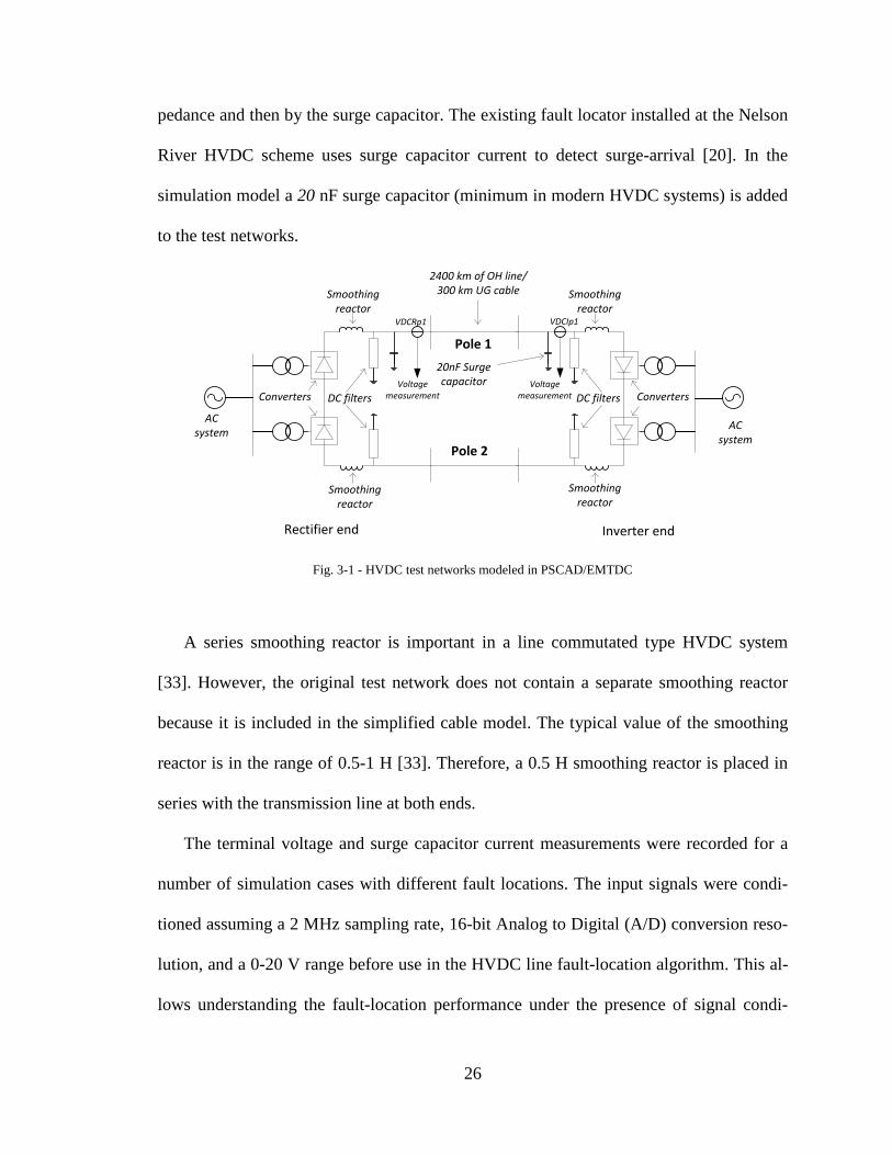
pedance and then by the surge capacitor. The existing fault locator installed at the Nelson
River HVDC scheme uses surge capacitor current to detect surge-arrival [20]. In the
simulation model a 20 nF surge capacitor (minimum in modern HVDC systems) is added
to the test networks.
Fig. 3-1 - HVDC test networks modeled in PSCAD/EMTDC
A series smoothing reactor is important in a line commutated type HVDC system
[33]. However, the original test network does not contain a separate smoothing reactor
because it is included in the simplified cable model. The typical value of the smoothing
reactor is in the range of 0.5-1 H [33]. Therefore, a 0.5 H smoothing reactor is placed in
series with the transmission line at both ends.
The terminal voltage and surge capacitor current measurements were recorded for a
number of simulation cases with different fault locations. The input signals were condi-
tioned assuming a 2 MHz sampling rate, 16-bit Analog to Digital (A/D) conversion reso-
lution, and a 0-20 V range before use in the HVDC line fault-location algorithm. This al-
lows understanding the fault-location performance under the presence of signal condi-
20nF Surge capacitor
Inverter end
Smoothing reactor
DC filters Converters
2400 km of OH line/300 km UG cable
AC system
VDCRp1 VDCIp1
Smoothing reactor
Rectifier end
Smoothing reactor
DC filtersConverters
Smoothing reactor
AC system
Pole 1
Pole 2
Voltage measurement
Voltage measurement
26
tioning required for digital processing. These A/D parameters were selected after careful
testing and considering the capabilities of the commercially available A/D converters.
Fig. 3-2 - HVDC dc line parameters (Left: OH line tower structure and Right: UG cable parameters)
3.2.1 HVDC test network with 2400 km long OH dc line
Fig. 3-3 shows monitored signals when a permanent dc line fault occurred 100 km
away from the rectifier terminal. Fig. 3-3 (a) and (b) show the original terminal voltage
and surge capacitor current measurements. The fault initiated surge is first observed at the
rectifier end, since the fault is much closer to the rectifier terminal.
The waveforms shown in Fig. 3-3 (c) and (d) are the measured terminal voltages and
surge capacitor currents respectively after normalization between 0-20 V and quantiza-
tion with a 16-bit resolution at a 2 MHz sampling rate. The input vector limits are taken
as 0-2 pu for voltage and -1 kA to 1 kA for surge capacitor currents. Therefore values be-
low zero are set to ‘zero’ due to the normalization effect as seen in voltage waveforms in
28.3
5
4.27
5.79
4.27
13.41
1
0.4
Outer radius (m)
Resistivity (Ω/m)
Relative permittivity
Conductor 0.03 1.72E-08 - Insulator 1 0.07 - 4.10 Sheath 0.07 1.72E-08 - Insulator 2 0.08 - 2.30
27
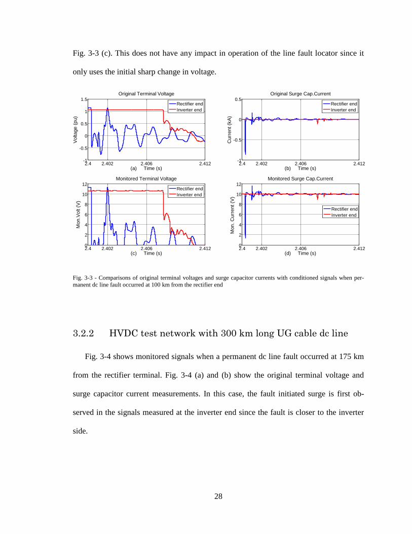
Fig. 3-3 (c). This does not have any impact in operation of the line fault locator since it
only uses the initial sharp change in voltage.
Fig. 3-3 - Comparisons of original terminal voltages and surge capacitor currents with conditioned signals when per-manent dc line fault occurred at 100 km from the rectifier end
3.2.2 HVDC test network with 300 km long UG cable dc line
Fig. 3-4 shows monitored signals when a permanent dc line fault occurred at 175 km
from the rectifier terminal. Fig. 3-4 (a) and (b) show the original terminal voltage and
surge capacitor current measurements. In this case, the fault initiated surge is first ob-
served in the signals measured at the inverter end since the fault is closer to the inverter
side.
2.4 2.402 2.406 2.412-1
-0.5
0
0.5
1
1.5Original Terminal Voltage
(a) Time (s)
Volta
ge (p
u)
Rectifier endInverter end
2.4 2.402 2.406 2.412-1
-0.5
0
0.5Original Surge Cap.Current
(b) Time (s)
Cur
rent
(kA)
Rectifier endInverter end
2.4 2.402 2.406 2.4120
2
4
6
8
10
12Monitored Terminal Voltage
(c) Time (s)
Mon
.Vol
t (V)
Rectifier endInverter end
2.4 2.402 2.406 2.4120
2
4
6
8
10
12Monitored Surge Cap.Current
(d) Time (s)
Mon
. Cur
rent
(V)
Rectifier endInverter end
28

Fig. 3-4 - Comparisons of original terminal voltages and surge capacitor currents with conditioned signals when per-manent dc line fault occurred at 175 km from the rectifier end (300 km UG cable HVDC test network)
The waveforms shown in Fig. 3-4 (c) and (d) are the measured terminal voltages and
surge capacitor currents respectively after normalization between 0-20 V and quantiza-
tion with a 16-bit resolution at a 2 MHz sampling rate. Similar to the OH line case, the
input vector limits are taken as 0-2 pu for voltage and -1 kA to 1 kA for surge capacitor
currents. However in this case there is no value below zero since the lower voltage drop
is seen compared to the OH line simulation results.
3.3 Wavelet based surge-arrival time detection
This section analyses the use of wavelet coefficients of the measured signals to detect
surge-arrival times.
2.4 2.401 2.4015 2.4021.03
1.04
1.05
1.06
1.07Original Terminal Voltage
(a) Time (s)
Volta
ge (p
u)
Rectifier endInverter end
2.4 2.401 2.4015 2.402-20
-15
-10
-5
0
5 x 10⁻³ Original Surge Cap.Current
(b) Time (s)
Cur
rent
(kA)
Rectifier endInverter end
2.4 2.401 2.4015 2.40210.3
10.4
10.5
10.6
10.7Monitored Terminal Voltage
(c) Time (s)
Mon
.Vol
t
Rectifier endInverter end
2.4 2.401 2.4015 2.4029.8
9.85
9.9
9.95
10
10.05Monitored Surge Cap.Current
(d) Time (s)
Mon
. Cur
rent
Rectifier endInverter end
29
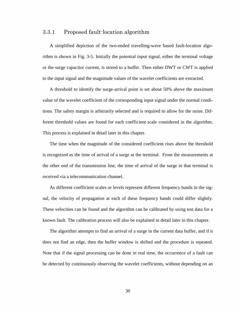
3.3.1 Proposed fault-location algorithm
A simplified depiction of the two-ended travelling-wave based fault-location algo-
rithm is shown in Fig. 3-5. Initially the potential input signal, either the terminal voltage
or the surge capacitor current, is stored to a buffer. Then either DWT or CWT is applied
to the input signal and the magnitude values of the wavelet coefficients are extracted.
A threshold to identify the surge-arrival point is set about 50% above the maximum
value of the wavelet coefficient of the corresponding input signal under the normal condi-
tions. The safety margin is arbitrarily selected and is required to allow for the noise. Dif-
ferent threshold values are found for each coefficient scale considered in the algorithm.
This process is explained in detail later in this chapter.
The time when the magnitude of the considered coefficient rises above the threshold
is recognized as the time of arrival of a surge at the terminal. From the measurements at
the other end of the transmission line, the time of arrival of the surge in that terminal is
received via a telecommunication channel.
As different coefficient scales or levels represent different frequency bands in the sig-
nal, the velocity of propagation at each of these frequency bands could differ slightly.
These velocities can be found and the algorithm can be calibrated by using test data for a
known fault. The calibration process will also be explained in detail later in this chapter.
The algorithm attempts to find an arrival of a surge in the current data buffer, and if it
does not find an edge, then the buffer window is shifted and the procedure is repeated.
Note that if the signal processing can be done in real time, the occurrence of a fault can
be detected by continuously observing the wavelet coefficients, without depending on an
30
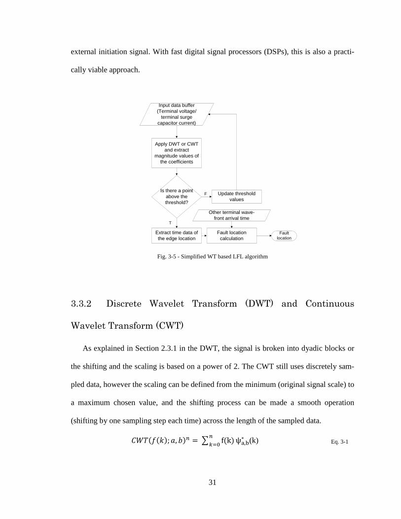
external initiation signal. With fast digital signal processors (DSPs), this is also a practi-
cally viable approach.
Fig. 3-5 - Simplified WT based LFL algorithm
3.3.2 Discrete Wavelet Transform (DWT) and Continuous
Wavelet Transform (CWT)
As explained in Section 2.3.1 in the DWT, the signal is broken into dyadic blocks or
the shifting and the scaling is based on a power of 2. The CWT still uses discretely sam-
pled data, however the scaling can be defined from the minimum (original signal scale) to
a maximum chosen value, and the shifting process can be made a smooth operation
(shifting by one sampling step each time) across the length of the sampled data.
𝐶𝑊𝑇(𝑓(𝑘);𝑎, 𝑏)𝑛 = f(k)𝑛𝑘=0 ψa,b
∗ (k) Eq. 3-1
Apply DWT or CWT and extract
magnitude values of the coefficients
Input data buffer(Terminal voltage/
terminal surge capacitor current)
Is there a point above the threshold?
Extract time data of the edge location
Update threshold values
Fault location
Fault location calculation
Other terminal wave-front arrival time
F
T
31

𝜓∗𝑎,𝑏(𝑘) =
1√𝑎
𝜓 𝑘 − 𝑏𝑎
Eq. 3-2
In Eq. 3-2 a and b are integers. The effect of discretizing the wavelet is that the time-
scale space is now sampled at discrete intervals. The sample number is represented by k
in both Eq. 3-1 and Eq. 3-2. In Eq. 3-1 the CWT coefficient is found for a sample win-
dow of interest which is denoted by n.
CWT provides a finer time and frequency resolution, and expects to perform better in
fault-location applications. The trade-off for this improved resolution is increased compu-
tational time and memory required to calculate the wavelet coefficients. However, HVDC
line fault-location is not a real time process and therefore, computational time is not a
critical issue. A description of the calculation of wavelet transform coefficients is given
in Appendix-A.
3.3.3 Application to a sample waveform
Examples of the terminal voltage and the surge capacitor current waveforms observed
during an HVDC line fault are shown in Fig. 3-6. All waveforms are sampled at a rate of
2 MHz and the OH transmission line is 2400 km long. Plot in Fig. 3-6 (a) shows the ter-
minal waveforms when a permanent line-to-ground fault occurred 625 km away from the
rectifier end. In this case, sharp drops in the voltages and the spikes in the surge capaci-
tors are clearly visible on both sides. Plot in Fig. 3-6 (b) shows the case when the fault
occurred 100 km from the rectifier terminal. First, the rectifier end sees a sharp drop in
the voltage when the initial surge arrived. The subsequent ripples seen on the rectifier
voltage are due to the reflected travelling waves. The magnitudes of the initial sharp volt-
age drop and the reflected surges are small on the inverter-side voltage for this case.
32

(a)
(b)
(c)
Fig. 3-6 - Terminal voltages and surge capacitor currents when permanent dc line fault occurred at (a) 625 km (b) 100 km (c) 2100 km from the rectifier end
Also, the magnitude of the surge observed at the inverter-side surge capacitor current
is much smaller compared to the rectifier side. This is due to the attenuation of travelling
2.4 2.402 2.406 2.412-0.5
0
0.5
1
1.5Terminal Voltage
Time (s)
Vol
tage
(pu)
Rectifier endInverter end
2.4 2.402 2.406 2.412-0.4
-0.3
-0.2
-0.1
0
0.1Surge Cap.Current
Time (s)
Cur
rent
(kA
)
Rectifier endInverter end
2.4 2.402 2.406 2.412-1
-0.5
0
0.5
1
1.5Terminal Voltage
Time (s)
Vol
tage
(pu)
Rectifier endInverter end
2.4 2.402 2.406 2.412-1
-0.8
-0.6
-0.4
-0.2
0
0.2
0.4Surge Cap.Current
Time (s)
Cur
rent
(kA
)
Rectifier endInverter end
2.4 2.402 2.406 2.412-1
-0.5
0
0.5
1
1.5Terminal Voltage
Time (s)
Vol
tage
(pu)
Rectifier endInverter end
2.4 2.402 2.406 2.412-0.6
-0.5
-0.4
-0.3
-0.2
-0.1
0
0.1Surge Cap.Current
Time (s)
Cur
rent
(kA
)
Rectifier endInverter end
33
waves when it travels along the transmission line. Plot in Fig. 3-6 (c) shows the wave-
forms when the fault is closer to the other end (2100 km from the rectifier terminal). In
this case the first sharp drop and the ripples due to reflections in the voltage are clearly
visible at the inverter side. The spike in the surge capacitor current at the rectifier side is
smaller than that of the inverter side. Thus it becomes more difficult to accurately detect a
surge when the fault is far from the measuring point.
Comparison of the DWT and CWT coefficient magnitude values for the waveforms
shown in Fig. 3-6 (a) is shown in Fig. 3-7. Here it is interesting to observe the surge de-
tection performance. Therefore, only the rectifier end terminal voltage and surge capaci-
tor measurements are analysed.
Plots in Fig. 3-7 (a) and Fig. 3-7 (f) show the rectifier end terminal voltage and surge
capacitor current respectively monitored from the simulations. Although the surge ap-
pears as a step change in voltage/surge capacitor current in the time scale used in Fig. 3-6
(a), when the time scale is expanded it appears as a smooth change. This explains the dif-
ficulty in locating the precise surge-arrival time. CWT of the terminal voltage is calcu-
lated with the Haar mother-wavelet at scales 4, 8, 16 and 32 and the magnitudes of these
coefficients are shown in Fig. 3-7 (b), (c), (d) and (e) respectively. DWT of the same sig-
nal is calculated with the Haar mother-wavelet for levels 2, 3, 4 and 5 (which are equiva-
lent to selected CWT scale values in frequency bands). Magnitudes of the detail coeffi-
cients of DWT are also shown in Fig. 3-7 (b), (c), (d) and (e) respectively. Similarly us-
ing the terminal surge capacitor current, CWT and DWT coefficient values are compared
in Fig. 3-7 (g), (h), (i) and (j).
34

Fig. 3-7 - DWT and CWT coefficient magnitude values of rectifier end voltage and surge capacitor current when a line to ground fault occurred (625 km away from the rectifier end applied at 2.4 s)
As can be seen from Fig. 3-7, the arrival of the surge is observed better in the wavelet
coefficients when compared to the original voltage signal. If a proper threshold value is
set, then the initial surge-arrival point can be detected by using the wavelet coefficients.
This process will be explained with more details in Section 3.3.5. Further, it is clearly
visible that the corresponding DWT values are poor in time resolution and also are
smaller in magnitude compared with CWT coefficients. Because of this reason, the CWT
2.40208 2.40211 2.402140
10
20
(a) Time(s)
Rec
. ter
. vol
t.
2.40208 2.40211 2.402140
0.2
0.4
(b) Time(s)
Coe
f. m
ag.
CWT S-4DWT L-2
2.40208 2.40211 2.402140
0.5
1
(c) Time(s)
Coe
f. m
ag.
CWT S-8DWT L-3
2.40208 2.40211 2.402140
2
4
(d) Time(s)
Coe
f. m
ag.
CWT S-16DWT L-4
2.40208 2.40211 2.402140
5
10
(e) Time(s)
Coe
f. m
ag.
CWT S-32DWT L-5
2.40208 2.4021 2.402126
8
10
(f) Time(s)Rec
. sur
. cap
. cur
.
2.40208 2.4021 2.402120
0.5
(g) Time(s)
Coe
f. m
ag.
CWT S-4DWT L-2
2.40208 2.4021 2.402120
1
2
(h) Time(s)
Coe
f. m
ag.
CWT S-8DWT L-3
2.40208 2.4021 2.402120
2
4
(i) Time(s)
Coe
f. m
ag.
CWT S-16DWT L-4
2.40208 2.4021 2.402120
5
10
(j) Time(s)
Coe
f. m
ag.
CWT S-32DWT L-5
35
based fault-location method can be expected to give better accuracy than the DWT based
fault-location method. Also, there is a time delay, which increases with the level/scale of
the coefficient, associated with the process of calculation of wavelet coefficients. How-
ever, this delay should not adversely affect the fault-location if the coefficients of the
same level/scale are used at the both ends because only the time differences are used in
the equations calculating the fault-location. However, larger errors can be expected at
higher levels/scales because the sharpness of the transients seen on the wavelet coeffi-
cients becomes lower at higher levels/scales.
Similar comparison is done when the fault happened 2100 km away from the rectifier
end and the results are shown in Fig. 3-8. Conditioned terminal voltage and surge-
capacitor current signals are shown in Fig. 3-8 (a) and Fig. 3-8 (f). As can be seen in the
figure, when the fault is far from the terminal, the changes in the monitored signals are
smaller. However, arrival of the surge is observed better in the wavelet coefficients when
compared to the original voltage signal.
36

Fig. 3-8- DWT and CWT coefficient magnitude values of rectifier end voltage and surge capacitor current when a line to ground fault occurred (2100 km away from the rectifier end applied at 2.4 s)
Further results are shown in Fig. 3-9 when the fault happened 100 km away from the
rectifier end. Conditioned terminal voltage and surge-capacitor current signals are shown
in Fig. 3-9 (a) and (f). As can be seen in the figure, when the fault is closer to the termi-
nal, the changes in the monitored signals are sharper. It can be clearly seen that the corre-
sponding DWT values are poor in time resolution and also are smaller in magnitude
compared with CWT coefficients.
2.407 2.407125 2.407255
10
15
(a) Time(s)
Rec
. ter
. vol
t.
2.407 2.407125 2.407250
0.1
0.2
(b) Time(s)
Coe
f. m
ag.
CWT S-4DWT L-2
2.407 2.407125 2.407250
0.2
0.4
(c) Time(s)
Coe
f. m
ag.
CWT S-8DWT L-3
2.407 2.407125 2.407250
0.5
1
(d) Time(s)
Coe
f. m
ag.
CWT S-16DWT L-4
2.407 2.407125 2.407250
2
4
(e) Time(s)
Coe
f. m
ag.
CWT S-32DWT L-5
2.407 2.407125 2.407258
10
12
(f) Time(s)
Rec
. sur
. cap
. cur
.
2.407 2.407125 2.407250
0.05
0.1
(g) Time(s)
Coe
f. m
ag.
CWT S-4DWT L-2
2.407 2.407125 2.407250
0.1
0.2
(h) Time(s)C
oef.
mag
.
CWT S-8DWT L-3
2.407 2.407125 2.407250
0.5
(i) Time(s)
Coe
f. m
ag.
CWT S-16DWT L-4
2.407 2.407125 2.407250
1
2
(j) Time(s)
Coe
f. m
ag.
CWT S-32DWT L-5
37

Fig. 3-9 - DWT and CWT coefficient magnitude values of rectifier end voltage and surge capacitor current when a line to ground fault occurred (100 km away from the rectifier end applied at 2.4 s)
3.3.4 Effect of mother-wavelet type
As mentioned before, the accuracy of the travelling-wave based line fault-location is
largely dependent on the precise identification of the surge-arrival time. The mother
wavelet plays an important role when wavelet transform is used to detect the surge-
arrival time. Selection of the proper mother wavelet type is a trial and error study. Moni-
tored rectifier end voltage, when a permanent dc line-to-ground fault applied at 625 km
away from the rectifier end, is used to analyze the effect of the mother wavelet. This
2.40033 2.400345 2.400360
10
20
(a) Time(s)
Rec
. ter
. vol
t.
2.40033 2.400345 2.400360
0.5
1
(b) Time(s)
Coe
f. m
ag.
CWT S-4DWT L-2
2.40033 2.400345 2.400360
2
4
(c) Time(s)
Coe
f. m
ag.
CWT S-8DWT L-3
2.40033 2.400345 2.400360
5
10
(d) Time(s)
Coe
f. m
ag.
CWT S-16DWT L-4
2.40033 2.400345 2.400360
10
20
(e) Time(s)
Coe
f. m
ag.
CWT S-32DWT L-5
2.40033 2.400345 2.400360
5
10
(f) Time(s)
Rec
. sur
. cap
. cur
.
2.40033 2.400345 2.400360
5
10
(g) Time(s)
Coe
f. m
ag.
CWT S-4DWT L-2
2.40033 2.400345 2.400360
5
10
(h) Time(s)
Coe
f. m
ag.
CWT S-8DWT L-3
2.40033 2.400345 2.400360
10
20
(i) Time(s)
Coe
f. m
ag.
CWT S-16DWT L-4
2.40033 2.400345 2.400360
10
20
(j) Time(s)
Coe
f. m
ag.
CWT S-32DWT L-5
38

waveform is shown in Fig. 3-10 (a) and the CWT coefficient magnitude values of that
waveform extracted using Daubechie family mother-wavelets are shown in Fig. 3-10 (b).
The Haar mother-wavelet (db 1) provides faster response and the sharpest edge com-
pared with other mother wavelets. Furthermore, it is the simplest mother wavelet and
therefore it requires less computational burden in the hardware implementation. There-
fore, the Haar mother-wavelet is selected in future studies in the wavelet-based line fault
locator.
Fig. 3-10 - Comparison coefficient magnitudes of different mother wavelets
(a) Rectifier end terminal voltage (b) Wavelet coefficient magnitudes when a line to ground fault occurred (625 km away from the rectifier end applied at 2.4 s)
2.402088 2.4020965 2.4021057
8
9
10
11
12
(a) Time(s)
Rec
. ter
. vol
t.
2.402088 2.4020965 2.4021050
0.002
0.004
0.006
0.008
0.01
(b) Time(s)
Coe
f. m
ag.
Haar db2 db4
db8
39

3.3.5 Effect of sampling frequency
Travelling-wave based line fault-location requires a high sampling frequency. This is
one of the major drawbacks in this method. However, the selection of a suitable sampling
frequency is a trade-off between the required accuracy and the availability of signal pro-
cessing and transducer hardware.
Fig. 3-11can be used to demonstrate the effect of sampling frequency in the accuracy
of the fault-location method. Fig. 3-11(a) shows the discretized simulated waveform of
the rectifier end voltage. Each sample is available when the waveform is sampled at a 2
MHz frequency. Red dots show the samples available when the waveform is sampled at a
1 MHz frequency. The green and black dots represent the samples when the waveform is
sampled at either 500 kHz or 400 kHz frequencies respectively. It is clear when the sam-
pling frequency is reduced the information available in a certain time period is reduced.
Travelling waves propagate along OH lines with a velocity equal to 300000 km/s and
along UG cables with a velocity approximately half of that. Therefore the wave travels in
the OH line about 300 m and in the UG cable about 150 m within a 1µs time period. If
the distance between samples is 1 µs or in other words the sampling frequency is 1 MHz,
then there is a possibility of error of about 300 m or 150 m in the OH line or in UG cable
respectively. Therefore it is clear how the accuracy of the fault-location is reduced when
the sampling frequency is reduced.
40

Fig. 3-11 - Effect of sampling frequency
Furthermore, Fig. 3-11(b)-(e) shows the CWT coefficient magnitude values taken
with the input signal shown Fig. 3-11 (a) at different sampling frequencies. Similar fre-
quency bands are used in the plots in order to match the CWT scale frequencies at differ-
ent sampling rate. For example scale 32 at a 2 MHz sampling frequency is representing
the 31.25 kHz to 62.5 kHz frequency band and scale 16 at a 1 MHz frequency is repre-
senting the same frequency band.
2.402075 2.4020875 2.40218
10
12
(a) Time(s)
Rec
. ter
. vol
t.
2.402075 2.4020875 2.40210
0.05
0.1
(b) Time(s)
|CW
T|
X: 2.402082003Y: 0.0181267932
2MHz CWT S-32
2.402075 2.4020875 2.40210
0.05
0.1
(c) Time(s)
|CW
T| X: 2.4020835Y: 0.03372243839
1MHz CWT S-16
2.402075 2.4020875 2.40210
0.5
1
(d) Time(s)
|CW
T|
X: 2.4020875Y: 0.01419089036
500kHz CWT S-4
2.402075 2.4020875 2.40210
0.5
(e) Time(s)
|CW
T|
X: 2.4020895Y: 0.01855838351
400kHz CWT S-2
41
The threshold is selected for each CWT magnitude scale, considering a safety margin
of 50% to the steady state maximum value. It is shown by the red line in each plot of the
CWT coefficient magnitude. The identified surge-arrival time is marked on each plot.
The fastest surge-arrival time is seen at the highest sampling frequency as 2.402082 s.
3.3.6 Determination of propagation velocity
In order to achieve good accuracy from the fault-location algorithm, it is important to
use accurate propagation velocity values, which are dependent on the configuration of the
OH line or UG cable in the HVDC system. Although it is possible to estimate the propa-
gation velocities from the conductor or cable geometry, the best approach is to estimate
these values using the measurements obtained for a known fault-location. Such data is
normally obtained during the commissioning of a line-fault location system.
During the test, a permanent dc line fault is applied at a known location. Then the
Wavelet coefficient magnitudes are extracted from the monitored terminal measurements.
Only the CWT coefficient values are shown for this test result. Surge-arrival times at the
two terminals are found using the pre-defined threshold values. Propagation velocity can
be calculated for each CWT scale using the Eq. 3-3.
𝑉 =𝐿 − 2𝑋𝑡𝑑
Eq. 3-3
Where L is the total line length, X is the test fault-location and td is the difference be-
tween the surge-arrival times at the two terminals found using the CWT coefficients.
As an example, a test fault is simulated at 400 km from the rectifier terminal of the
test network with 2400 km of the OH line. Table 3-1 shows the calculated propagation
velocities using the wavelet coefficients at different scales. As can be seen, lower scales
42
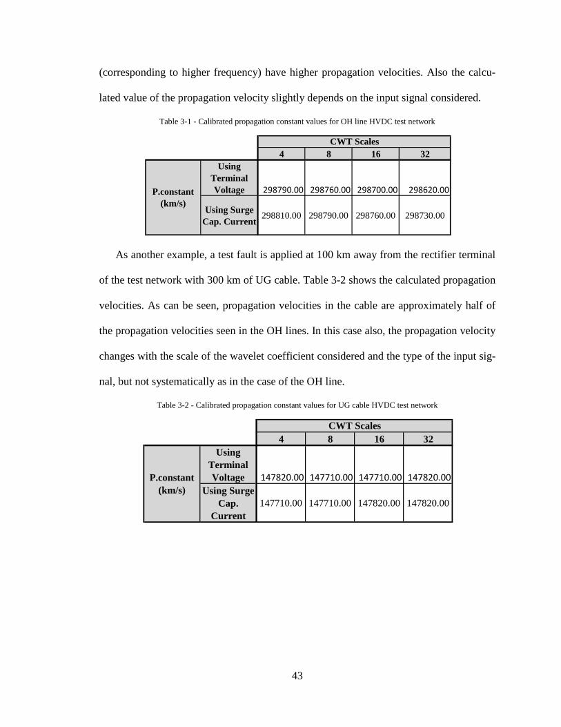
(corresponding to higher frequency) have higher propagation velocities. Also the calcu-
lated value of the propagation velocity slightly depends on the input signal considered.
Table 3-1 - Calibrated propagation constant values for OH line HVDC test network
As another example, a test fault is applied at 100 km away from the rectifier terminal
of the test network with 300 km of UG cable. Table 3-2 shows the calculated propagation
velocities. As can be seen, propagation velocities in the cable are approximately half of
the propagation velocities seen in the OH lines. In this case also, the propagation velocity
changes with the scale of the wavelet coefficient considered and the type of the input sig-
nal, but not systematically as in the case of the OH line.
Table 3-2 - Calibrated propagation constant values for UG cable HVDC test network
4 8 16 32Using
Terminal Voltage 298790.00 298760.00 298700.00 298620.00
Using Surge Cap. Current 298810.00 298790.00 298760.00 298730.00
CWT Scales
P.constant (km/s)
4 8 16 32Using
Terminal Voltage 147820.00 147710.00 147710.00 147820.00
Using Surge Cap.
Current147710.00 147710.00 147820.00 147820.00
CWT Scales
P.constant (km/s)
43

3.4 Simulation results for HVDC systems with
extra-long dc line
The results of the dc line fault-location with wavelet coefficients are presented for the
two test networks, the HVDC system with a 2400 km long OH line and the HVDC sys-
tem with a 300 km long UG cable. The simulation tests were designed to
• compare the fault-location performance with two potential input signals consid-
ered, (i) the converter terminal voltages and (ii) the surge capacitor currents.
• compare the fault-location performance with DWT and CWT coefficients of the
input signals
• identify the most suitable scales/levels of the wavelet coefficients
• investigate the effect of noise and identify the best parameters under the presence
of noise.
The fault-location performance was evaluated using the absolute prediction error.
This value shows the magnitude difference between the predicted fault-location and the
actual fault-location in kilometers.
3.4.1 Simulation results: HVDC test network - 2400 km OH
line
Table 3-3 and Fig. 3-12 show the fault-location results for different fault locations,
when the CWT coefficients of the terminal voltage measurements are used to identify the
travelling-wave arrival time. The prediction errors are within ±350 m for CWT scales up
to 32. In general the lower scales give better accuracy.
44

Table 3-3 - Fault-location results with different CWT coefficients (scales 4, 8, 16, and 32) of the terminal voltages
Actual fault-location
(km)
Predicted fault-location (in km) using CWT Scales
4 8 16 32
1 1.120 1.158 1.157 1.120
10 10.159 10.120 10.193 10.228
100 100.093 100.047 100.028 100.037
157 157.012 157.035 157.006 156.999
251 250.980 250.994 251.022 250.915
333 333.072 333.003 333.091 333.035
850 850.121 850.079 850.145 850.093
1111 1110.887 1110.821 1110.837 1110.713
1200 1200.000 1200.075 1200.075 1200.075
1323 1322.951 1323.014 1322.916 1323.031
1400 1400.037 1399.944 1399.907 1400.000
2040 2040.037 2040.034 2040.026 2040.090
2100 2099.869 2099.860 2099.767 2099.664
2240 2239.925 2239.903 2239.933 2239.866
Fig. 3-12 - Fault-location errors with different CWT coefficients (scale 4, 8, 16, and 32) of the terminal voltages
Table 3-4 and Fig. 3-13 show the fault-location results when the surge capacitor cur-
rents are used as the input signals. Overall accuracy is similar to the accuracy obtained
with the terminal voltages as inputs. The prediction errors are within ±400 m for the
1 10 100 157 251 333 400 850 1111 1200 1323 1400 2040 2100 22400
0.05
0.1
0.15
0.2
0.25
0.3
0.35
Actual fault location (km)
Abs
olut
e pr
edic
tion
erro
r (km
)
S:4S:8S:16S:32
45

CWT scales up to 32. Again, the lower scales give better accuracy. These results indicate
that both input signals, the surge capacitor current and the terminal voltage, work equally
well for fault locating in HVDC.
Table 3-4 - Fault-location results with different CWT coefficients (scale 4, 8, 16, and 32) of the surge capacitor currents
Actual fault-location
(km)
Predicted fault-location (in km) using CWT Scales
4 8 16 32
1 1.158 1.270 1.232 1.195
10 10.197 10.233 10.270 10.232
100 100.140 100.168 100.196 100.149
157 157.064 157.087 157.110 157.058
251 250.966 250.980 250.994 251.008
333 332.991 333.072 333.078 333.010
850 850.014 849.972 849.930 849.888
1111 1110.953 1110.962 1110.895 1110.829
1200 1200.000 1199.925 1199.851 1199.851
1323 1322.962 1322.951 1322.939 1322.853
1400 1399.981 1399.888 1399.869 1399.776
2040 2039.892 2039.888 2039.735 2039.731
2100 2099.879 2099.720 2099.711 2099.627
2240 2239.873 2239.776 2239.754 2239.656
Fig. 3-13 - Fault-location errors with different CWT coefficients (scales 4, 8, 16, and 32) of the surge capacitor currents
1 10 100 157 251 333 400 850 1111 1200 1323 1400 2040 2100 22400
0.05
0.1
0.15
0.2
0.25
0.3
0.35
0.4
Actual fault location (km)
Abs
olut
e pr
edic
tion
erro
r (km
)
S:4S:8S:16S:32
46

Table 3-5, Table 3-6, Fig. 3-14, and Fig. 3-15 summarize the fault-location perfor-
mance obtained when DWT coefficients of the input signals are used to detect the surge-
arrival times. In Fig. 3-14 the terminal voltages are used as the inputs for the fault-
location algorithm. According to the tested cases the prediction error is within ±2.5 km
when detail coefficients up to level 5 are used. Although smaller prediction errors are vis-
ible at lower DWT levels, these coefficients can be affected by noise.
Table 3-5 - Fault-location results with different DWT coefficients (levels 2, 3, 4, and 5) of the terminal voltages
Actual fault-location
(km)
Predicted fault-location (in km) using DWT levels
2 3 4 5
1 1.046 1.046 1.941 2.236
10 10.011 9.712 10.601 12.374
100 99.963 99.365 100.187 101.826
157 156.743 157.041 157.223 158.777
251 250.878 250.579 251.885 250.913
333 332.761 332.761 334.005 335.296
850 850.056 850.056 850.317 852.031
1111 1110.945 1110.945 1110.414 1110.548
1200 1200.000 1200.000 1200.000 1200.000
1323 1323.123 1323.422 1323.031 1324.338
1400 1400.224 1399.925 1399.179 1398.882
2040 2040.344 2040.344 2040.911 2039.955
2100 2100.112 2100.112 2099.440 2099.590
2240 2240.269 2240.269 2240.090 2238.539
47

Fig. 3-14 - Fault-location errors with different DWT coefficients (levels 2, 3, 4, and 5) of the terminal voltages
In Table 3-6 and Fig. 3-15, detail DWT coefficients of the surge capacitor currents
are used as inputs. The results indicate that the prediction errors less than ±2.2 km are
achievable for the tested cases using DWT levels up to 5. Again a better accuracy can be
achieved with lower detail levels.
Table 3-6 - Fault-location results with different DWT coefficients (levels 2, 3, 4, and 5) of the surge capacitor currents
Actual fault-location
(km)
Predicted fault-location (in km) using DWT levels
2 3 4 5
1 2.540 2.241 1.608 -1.083
10 11.505 9.712 9.083 9.083
100 99.963 99.963 98.783 98.783
157 157.041 157.041 155.892 156.191
251 250.878 250.579 250.675 250.675
333 333.059 333.358 332.900 332.900
850 850.056 850.056 849.871 848.675
1111 1110.945 1110.945 1111.496 1112.692
1200 1200.000 1199.402 1198.804 1200.000
1323 1322.824 1322.824 1323.487 1322.291
1400 1399.925 1399.925 1400.629 1399.433
2040 2040.045 2040.344 2040.788 2039.891
2100 2099.813 2100.112 2100.588 2099.691
2240 2239.970 2240.269 2241.417 2241.417
1 10 100 157 251 333 400 850 1111 1200 1323 1400 2040 2100 22400
0.5
1
1.5
2
2.5
Actual fault location (km)
Abs
olut
e pr
edic
tion
erro
r (km
)
L:2L:3L:4L:5
48
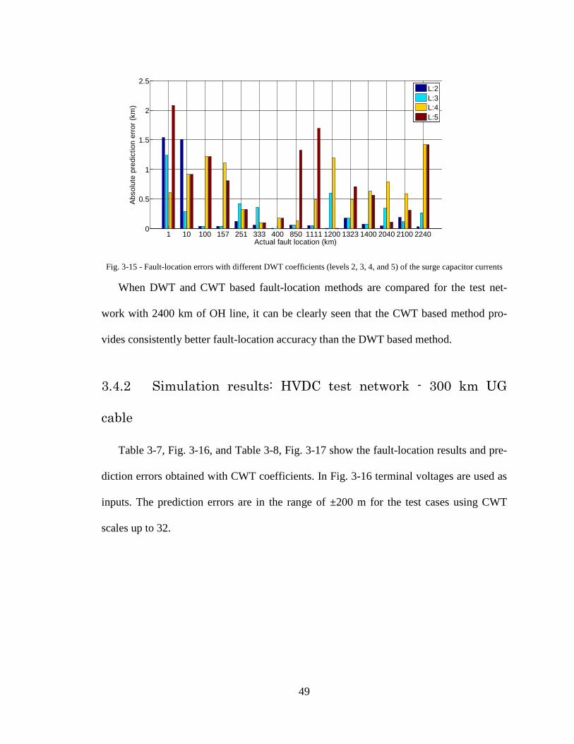
Fig. 3-15 - Fault-location errors with different DWT coefficients (levels 2, 3, 4, and 5) of the surge capacitor currents
When DWT and CWT based fault-location methods are compared for the test net-
work with 2400 km of OH line, it can be clearly seen that the CWT based method pro-
vides consistently better fault-location accuracy than the DWT based method.
3.4.2 Simulation results: HVDC test network - 300 km UG
cable
Table 3-7, Fig. 3-16, and Table 3-8, Fig. 3-17 show the fault-location results and pre-
diction errors obtained with CWT coefficients. In Fig. 3-16 terminal voltages are used as
inputs. The prediction errors are in the range of ±200 m for the test cases using CWT
scales up to 32.
1 10 100 157 251 333 400 850 1111 1200 1323 1400 2040 2100 22400
0.5
1
1.5
2
2.5
Actual fault location (km)
Abs
olut
e pr
edic
tion
erro
r (km
)
L:2L:3L:4L:5
49
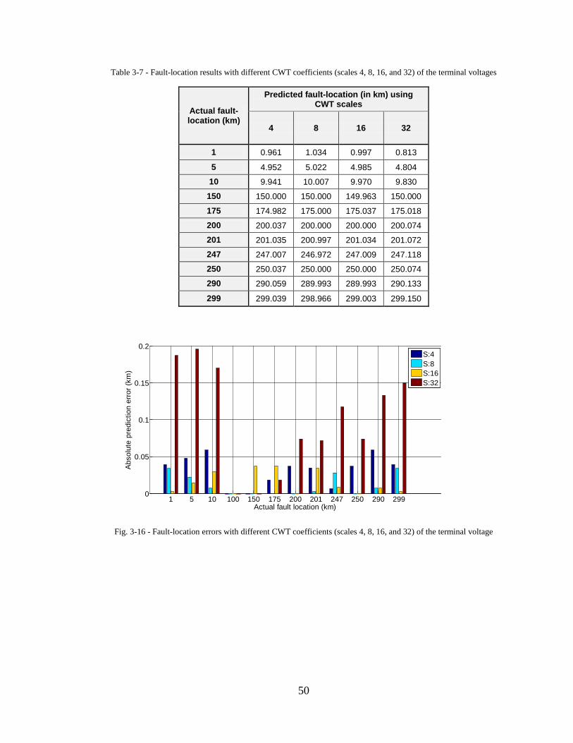
Table 3-7 - Fault-location results with different CWT coefficients (scales 4, 8, 16, and 32) of the terminal voltages
Actual fault-location (km)
Predicted fault-location (in km) using CWT scales
4 8 16 32
1 0.961 1.034 0.997 0.813
5 4.952 5.022 4.985 4.804
10 9.941 10.007 9.970 9.830
150 150.000 150.000 149.963 150.000
175 174.982 175.000 175.037 175.018
200 200.037 200.000 200.000 200.074
201 201.035 200.997 201.034 201.072
247 247.007 246.972 247.009 247.118
250 250.037 250.000 250.000 250.074
290 290.059 289.993 289.993 290.133
299 299.039 298.966 299.003 299.150
Fig. 3-16 - Fault-location errors with different CWT coefficients (scales 4, 8, 16, and 32) of the terminal voltage
1 5 10 100 150 175 200 201 247 250 290 2990
0.05
0.1
0.15
0.2
Actual fault location (km)
Abs
olut
e pr
edic
tion
erro
r (km
)
S:4S:8S:16S:32
50

Table 3-8 - Fault-location results with different CWT coefficients (scales 4, 8, 16, and 32) of the surge capacitor cur-
rents
Actual fault-location (km)
Predicted fault-location (in km) using CWT scales
4 8 16 32
1 1.182 1.145 1.035 0.998
5 5.170 5.133 5.026 4.989
10 10.155 10.118 10.015 9.978
150 150.000 150.000 150.000 150.000
175 174.963 174.963 174.982 174.982
200 200.000 199.963 200.000 200.000
201 200.960 200.960 200.998 201.035
247 246.861 246.935 247.007 247.007
250 249.889 249.889 249.963 250.000
290 289.845 289.882 289.985 290.022
299 298.818 298.818 298.965 299.002
Fault-location errors when surge capacitor currents were used as inputs are shown in
Fig. 3-17. Maximum prediction error values are within ±200 m for the CWT scale 4. The
overall prediction errors lie within the same range obtained with the terminal voltages.
Therefore, even for the UG cable based HVDC systems, the surge capacitor current can
be used as a potential input to this fault-location algorithm.
Fig. 3-17 - Fault-location errors with different CWT coefficients (scales 4, 8, 16, and 32) of the surge capacitor currents
1 5 10 100 150 175 200 201 247 250 290 2990
0.05
0.1
0.15
0.2
Actual fault location (km)
Abs
olut
e pr
edic
tion
erro
r (km
)
S:4S:8S:16S:32
51

Table 3-10 and Fig. 3-19 show the fault-location results obtained using DWT coeffi-
cients of the terminal voltages and the surge capacitor currents respectively. The predic-
tion errors are within the range of ±1.8 km in the case of terminal voltages and ±3.5 km
in the case of surge capacitor currents. Therefore, again it is clear that the CWT coeffi-
cient based method provides better overall accuracy than the DWT coefficient based
method. Furthermore, the results also indicate that the same algorithm can be used in
HVDC systems with UG cables.
Table 3-9 - Fault-location results with different DWT coefficients (levels 2, 3, 4, and 5) of the terminal voltages
Actual fault-location
(km)
Predicted fault-location (in km) using DWT levels
2 3 4 5
1 0.740 1.471 2.632 2.485
5 4.882 5.588 6.140 6.287
10 9.911 10.588 11.111 11.111
150 150.000 150.000 150.000 150.000
175 175.000 174.853 174.415 174.415
200 200.000 200.000 200.000 199.854
201 201.036 200.588 200.000 200.000
247 247.041 246.471 246.199 246.345
250 250.148 249.559 248.684 248.684
290 290.089 289.412 288.889 288.889
299 299.260 298.529 297.368 297.515
52

Fig. 3-18 - Fault-location results with different DWT coefficients (levels 2, 3, 4, and 5) of the terminal voltages
Table 3-10 - Fault-location results with different DWT coefficients (levels 2, 3, 4, and 5) of the surge capacitor currents
Actual fault-location
(km)
Predicted fault-location (in km) using
DWT levels
2 3 4 5
1 0.888 0.888 0.888 -1.048
5 5.030 4.734 4.438 2.844
10 10.059 9.763 9.467 6.587
150 150.000 150.000 150.000 150.000
175 175.000 175.000 174.704 175.000
200 200.000 200.000 200.000 201.048
201 201.036 201.183 201.183 201.198
247 247.041 247.041 247.337 248.653
250 250.000 250.148 249.852 251.048
290 289.941 290.237 290.533 293.413
299 299.112 299.112 299.112 301.048
1 5 10 100 150 175 200 201 247 250 290 2990
0.2
0.4
0.6
0.8
1
1.2
1.4
1.6
1.8
Actual fault location (km)
Abs
olut
e pr
edic
tion
erro
r (km
)
L:2L:3L:4L:5
53

Fig. 3-19 - Fault-location results with different DWT coefficients (levels 2, 3, 4, and 5) of the surge capacitor currents
3.5 Effect of the noise in the input signal
Performance of the fault-location algorithm was tested with input signals contaminat-
ed with uniformly distributed random noise. This study was done for both test networks.
As an example, Fig. 3-20 shows rectifier terminal voltage and surge capacitor current
contaminated with noise in the HVDC system with an OH dc line. In Fig. 3-20 (a), recti-
fier end voltage with added 0.001 pu white noise is compared with the clean signal. In
Fig. 3-20 (b), the same signal with 0.01 pu white noise is shown.
Fig. 3-20 (c) and (d) compare the rectifier end surge capacitor current with 0.001 kA
and 0.01 kA noise respectively with the clean signal. In the following sections, results
obtained with the CWT based method are presented for the two test networks.
1 5 10 100 150 175 200 201 247 250 290 2990
0.5
1
1.5
2
2.5
3
3.5
Actual fault location (km)
Abs
olut
e pr
edic
tion
erro
r (km
)
L:2L:3L:4L:5
54

Fig. 3-20 - Surge capacitor current and terminal voltage with added noise
3.5.1 Performance with noisy inputs: HVDC test network with
2400 km long OH dc line
The fault-location performance obtained with terminal voltage measurements contam-
inated with 0.005 pu noise and 0.001 pu noise is compared with the normal no noise con-
dition in Fig. 3-21. Similarly, Fig. 3-22 compares the prediction fault-location perfor-
mance obtained with surge capacitor current measurements contaminated with 0.005 kA
noise and 0.001 kA noise with the normal no noise condition.
2.4013 2.40134
1.13121.1322
Time(s)- (a)
Rec
. ter
. vol
t (pu
)
Noisy signalOriginal signal
1.125
1.13
1.135
Time(s) - (b)
Rec
. ter
. vol
t (pu
)
Noisy signalOriginal signal
-0.50.5
x 10-3
Time(s) - (c)
Rec
.Sur
.cap
.cur
(kA
)
Noisy signalOriginal signal
-5
0
5x 10⁻³
Time(s) - (d)R
ec.S
ur.c
ap.c
ur (k
A)
Noisy signalOriginal signal
55

Fig. 3-21 - Prediction errors for different noise levels in the terminal voltages (Using CWT Scale 4)
In both of these cases only the CWT scale 4 coefficients, which gave the lowest errors
in general, was used. According to the results, with increasing noise level, the accuracy of
the fault-location is reduced, although occasionally the errors are reduced due to compen-
sation of other errors by the random noise.
Fig. 3-22 - Prediction errors for different noise levels in the surge capacitor current measurements (Using CWT Scale 4)
Fig. 3-23 compares the prediction errors with different CWT scales when the terminal
voltages containing 0.005 pu noise are used as inputs. As can be seen in Fig. 3-23, the
lower scales are more sensitive to noise than the higher scales. Therefore when the input
1 10 100 157 251 333 400 850 1111 1200 1323 1400 2040 2100 22400
0.2
0.4
0.6
0.8
1
1.2
1.4
Actual fault location (km)
Abs
olut
e pr
edic
tion
erro
r (km
)
Nonoise0.001pu noise0.005pu noise
1 10 100 157 251 333 400 850 1111 1200 1323 1400 2040 2100 22400
0.2
0.4
0.6
0.8
1
1.2
1.4
Actual fault location (km)
Abs
olut
e pr
edic
tion
erro
r (km
)
Nonoise0.001kA noise0.005kA noise
56

signals are corrupted with noise, which is usually the case in practical situations, use of
higher CWT scales (Scales 16 and 32) is desirable to achieve robust results.
Fig. 3-23 - Comparison of prediction errors using different CWT scales for terminal voltage with 0.005pu of noise
3.5.2 Performance with noisy inputs: HVDC test network with
300 km long UG cable dc line
The results obtained for the UG cable test network are presented in Fig. 3-24 and Fig.
3-25. It was found that cable based test network is more sensitive to noise and therefore
higher scales (Scale 16) are used to compare fault location performance with changing
noise levels. Fig. 3-24 compares the prediction errors using terminal voltage measure-
ments contaminated with 0.001 pu noise and no noise. Fig. 3-25 compares the prediction
errors using surge capacitor measurements contaminated with 0.001 kA noise and no
noise.
It is clearly visible that the performance of the fault-location algorithm is sensitive to
noise in the input signal. In the case shown in Table 3-11, where the input signal is the
voltage contaminated with 0.001 pu noise, it was impossible to find the fault-location
1 10 100 157 251 333 400 850 1111 1200 1323 1400 2040 2100 22400
0.2
0.4
0.6
0.8
1
1.2
1.4
Actual fault location (km)
Abs
olut
e pr
edic
tion
erro
r (km
)
S:4S:8S:16S:32
57
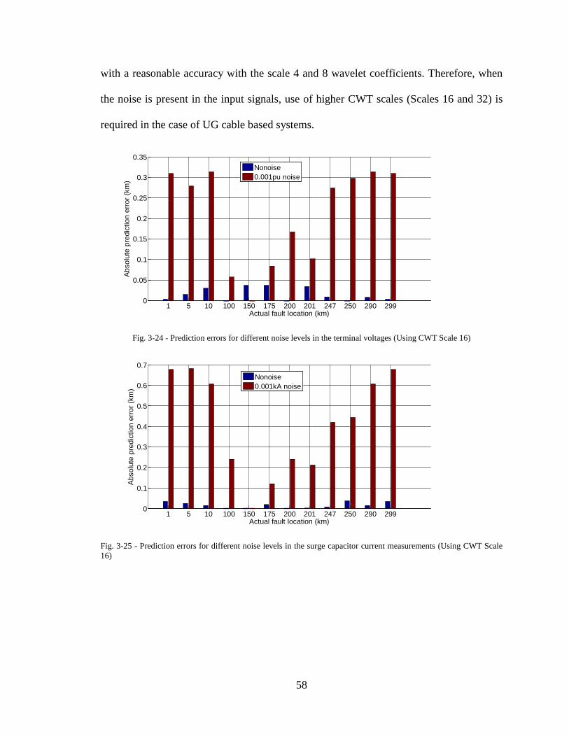
with a reasonable accuracy with the scale 4 and 8 wavelet coefficients. Therefore, when
the noise is present in the input signals, use of higher CWT scales (Scales 16 and 32) is
required in the case of UG cable based systems.
Fig. 3-24 - Prediction errors for different noise levels in the terminal voltages (Using CWT Scale 16)
Fig. 3-25 - Prediction errors for different noise levels in the surge capacitor current measurements (Using CWT Scale 16)
1 5 10 100 150 175 200 201 247 250 290 2990
0.05
0.1
0.15
0.2
0.25
0.3
0.35
Actual fault location (km)
Abs
olut
e pr
edic
tion
erro
r (km
)
Nonoise0.001pu noise
1 5 10 100 150 175 200 201 247 250 290 2990
0.1
0.2
0.3
0.4
0.5
0.6
0.7
Actual fault location (km)
Abs
olut
e pr
edic
tion
erro
r (km
)
Nonoise0.001kA noise
58
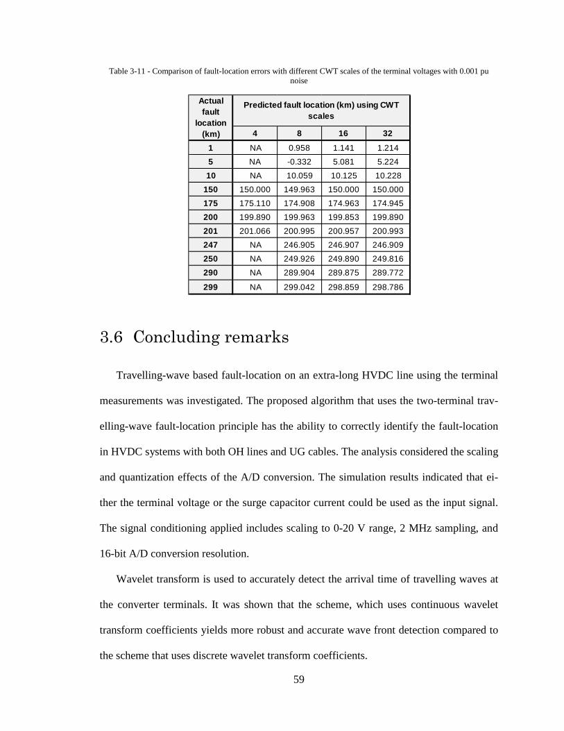
Table 3-11 - Comparison of fault-location errors with different CWT scales of the terminal voltages with 0.001 pu
noise
3.6 Concluding remarks
Travelling-wave based fault-location on an extra-long HVDC line using the terminal
measurements was investigated. The proposed algorithm that uses the two-terminal trav-
elling-wave fault-location principle has the ability to correctly identify the fault-location
in HVDC systems with both OH lines and UG cables. The analysis considered the scaling
and quantization effects of the A/D conversion. The simulation results indicated that ei-
ther the terminal voltage or the surge capacitor current could be used as the input signal.
The signal conditioning applied includes scaling to 0-20 V range, 2 MHz sampling, and
16-bit A/D conversion resolution.
Wavelet transform is used to accurately detect the arrival time of travelling waves at
the converter terminals. It was shown that the scheme, which uses continuous wavelet
transform coefficients yields more robust and accurate wave front detection compared to
the scheme that uses discrete wavelet transform coefficients.
4 8 16 32
1 NA 0.958 1.141 1.214
5 NA -0.332 5.081 5.224
10 NA 10.059 10.125 10.228
150 150.000 149.963 150.000 150.000
175 175.110 174.908 174.963 174.945
200 199.890 199.963 199.853 199.890
201 201.066 200.995 200.957 200.993
247 NA 246.905 246.907 246.909
250 NA 249.926 249.890 249.816
290 NA 289.904 289.875 289.772
299 NA 299.042 298.859 298.786
Actual fault
location (km)
Predicted fault location (km) using CWT scales
59

Application of the proposed fault-location method to two HVDC systems consisting
of a 2400 km long overhead line and a 300 km long underground cable were demonstrat-
ed through simulations. The simulation results verified the correct operation of the fault-
location algorithm. According to the simulation results, it was possible to achieve a fault-
location prediction error of ±400 m for the test system with a 2400 km OH line using ei-
ther terminal voltage or surge capacitor current measurements as inputs. The simulation
results also show this algorithm works with a 300 km UG cable line and both inputs sig-
nals would produce similar accuracy levels: in the prediction error range of ±200 m under
normal conditions for permanent line to ground faults.
Simulations showed that the proposed method’s accuracy degrades with the presence
of measurement noise. It was found that the UG cable test network is more sensitive to
noise than the OH line test network. However, when the noise is present in the input sig-
nals, use of higher CWT scales (Scales 16 and 32) is desirable to achieve robust results in
both test networks.
60

Chapter 4
Fault-location in conventional HVDC
schemes with multiple segments
4.1 Introduction
HVDC transmission systems are often used to transport electricity across water bod-
ies such as rivers, lakes, and seas where underground, underwater or submarine cables are
used. Since converter stations are not always located close to the shore of the water body,
these HVDC systems use a combination of OH transmission and UG cables as the trans-
mission medium. Such intricate configurations are becoming an integral part of HVDC
systems [18], [34]. Existing travelling-wave-based dc line fault-location methods have
been developed for the HVDC systems with only OH transmission lines or only UG ca-
ble. Fault-location in HVDC systems with combination of overhead lines and cables has
been generally achieved by considering each line section separately. However, this prac-
tice is expensive, as it requires duplicate installation of additional hardware at both ends
of each section.
61
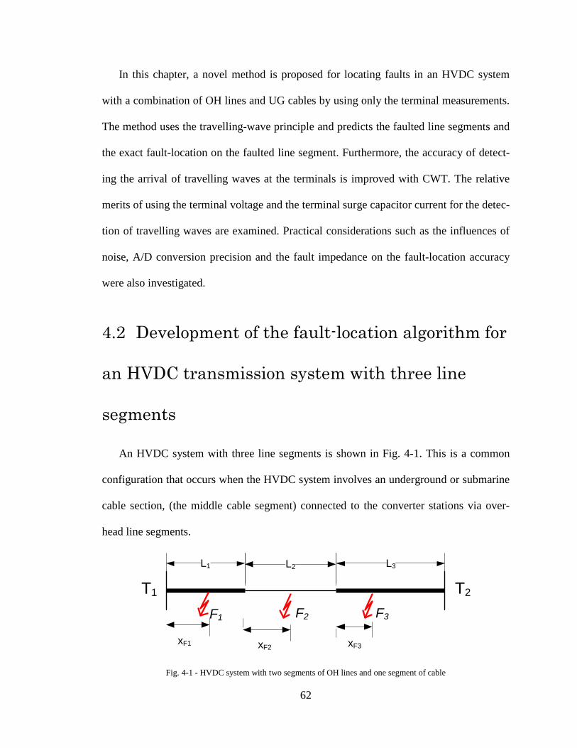
In this chapter, a novel method is proposed for locating faults in an HVDC system
with a combination of OH lines and UG cables by using only the terminal measurements.
The method uses the travelling-wave principle and predicts the faulted line segments and
the exact fault-location on the faulted line segment. Furthermore, the accuracy of detect-
ing the arrival of travelling waves at the terminals is improved with CWT. The relative
merits of using the terminal voltage and the terminal surge capacitor current for the detec-
tion of travelling waves are examined. Practical considerations such as the influences of
noise, A/D conversion precision and the fault impedance on the fault-location accuracy
were also investigated.
4.2 Development of the fault-location algorithm for
an HVDC transmission system with three line
segments
An HVDC system with three line segments is shown in Fig. 4-1. This is a common
configuration that occurs when the HVDC system involves an underground or submarine
cable section, (the middle cable segment) connected to the converter stations via over-
head line segments.
Fig. 4-1 - HVDC system with two segments of OH lines and one segment of cable
L2L1 L3
F1
xF1 xF2 xF3
T1 T2
F2 F3
62

The lengths of the segments are L1, L2 and L3 respectively. Faults F1, F2 and F3 lo-
cated on Segments 1, 2, and 3 respectively are used to explain the fault-location concept.
The distance to a fault is calculated from the beginning of the faulted segment. For exam-
ple, xF1 is the distance to fault F1 in Segment 1 from the terminal T1, and xF2 is the dis-
tance to fault F2 from the beginning of Segment 2.
Consider the case of fault F1. If the fault occurs at time t=0, the time of arrival of the
travelling-wave at Terminal T1 is given by:
𝑡1−𝐹1 =𝑥𝐹1𝑣1
Eq. 4-1
Where v1 is the propagation velocity of the travelling-wave in segment 1. The arrival time
of the travelling-wave to terminal T2 for the same fault is given by:
𝑡2−𝐹1 = 𝐿1 − 𝑥𝐹1
𝑣1 +
𝐿2𝑣2
+𝐿3𝑣3
Eq. 4-2
Where v2 and v3 are the propagation velocities of the travelling-wave in segments 2 and 3
respectively. The difference between the arrival times Δt12-F1 can then be obtained as:
∆𝑡12−𝐹1 = 𝑡1−𝐹1 − 𝑡2−𝐹1 =2 ∙ 𝑥𝐹1𝑣1
−𝐿1𝑣1−𝐿2𝑣2−𝐿3𝑣3
Eq. 4-3
The distance to the fault from the beginning of segment 1 can be obtained from Eq.
4-3 as
𝑥𝐹1 = ∆𝑡12−𝐹1 +𝐿1𝑣1
+𝐿2𝑣2
+𝐿3𝑣3 ×
𝑣12
Eq. 4-4
If Δt12-F1 is obtained from the measurements, the fault can be located given the propa-
gation velocities in the three segments.
Now consider fault F2 that occurs in the middle segment at instant t=0. The respec-
tive surge-arrival times at terminals T1 and T2 are given by Eq. 4-5 and Eq. 4-6.
63

The difference between surge-arrival times Δt12-F2 is
This gives the fault-location with respect to the start of segment 2 as
𝑥𝐹2 = ∆𝑡12−𝐹2 −𝐿1𝑣1
+𝐿2𝑣2
+𝐿3𝑣3 ×
𝑣22
Eq. 4-8
Similarly, considering fault F3 on segment 3, it is possible to show that the distance to
fault F3 from the beginning of segment 3 is given by
𝑥𝐹3 = ∆𝑡12−𝐹3 −𝐿1𝑣1−𝐿2𝑣2
+𝐿3𝑣3 ×
𝑣32
Eq. 4-9
Where Δt12-F3 is difference between the surge-arrival times at terminals T1 and T2 for fault
F3.
4.3 Identification of the faulty line segment
In deriving the expressions for the distance to the fault given in Eq. 4-4, Eq. 4-8 and
Eq. 4-9, it was assumed that the segment where the fault is on is known. However, in
practical applications, this is not known. The only measurable quantity is the difference
between the surge-arrival times, Δt12. Thus, it is necessary to identify the faulted segment
before pinpointing the exact location of the fault. Fortunately, this can be easily achieved
by following the procedure described below.
𝑡1−𝐹2 =𝑥𝐹2𝑣2
+𝐿1𝑣1
Eq. 4-5
𝑡2−𝐹2 = 𝐿2 − 𝑥𝐹2
𝑣2 +
𝐿3𝑣3
Eq. 4-6
∆𝑡12−𝐹2 =2 ∙ 𝑥𝐹2𝑣2
+𝐿1𝑣1−𝐿2𝑣2−𝐿3𝑣3
Eq. 4-7
64

First, the value of Δt12 is obtained through the measurements. Then Eq. 4-4, Eq. 4-8
and Eq. 4-9 are applied to obtain three different values for the fault distance (correspond-
ing to xF1, xF2, and xF3). Next, the values of xF1, xF2, and xF3 are compared with the corre-
sponding segment lengths, L1, L2 and L3. It can be shown that if the calculated xFi value is
between zero and the segment length, Li, then the fault is in that segment. Furthermore,
only one of the three xFi values will satisfy the above condition for a given fault. Hence,
the faulted line segment can be identified without any ambiguity.
For example, consider a case where the fault is in Segment 2 (middle segment). The
actual difference between the surge-arrival times (which should be equal to the measured
Δt12) for this case can be obtained from Eq. 4-10 as
∆𝑡12 =2 ∙ 𝑥𝐹2𝑣2
+𝐿1𝑣1−𝐿2𝑣2−𝐿3𝑣3
Eq. 4-10
The estimated value of xF1, obtained by substituting the value of Δt12 into Eq. 4-4, is
𝑥𝐹1 = 𝐿1 + 𝑥𝐹2 ×𝑣1𝑣2
Eq. 4-11
Since the ratio of propagation velocities (v1/v2) is always greater than zero, the esti-
mated value of xF1 would be larger than L1 for this case, indicating that the fault is not on
Segment 1. Similarly, substitution of Δt12 from Eq. 4-10 (measured Δt12) into Eq. 4-11
gives,
𝑥𝐹3 = (𝑥𝐹2 − 𝐿2) ×𝑣3𝑣2
Since (v3/v2) is always greater than zero, and xF2 is smaller than L2, the estimated
value of xF3 for this case would be negative indicating that the fault is not on Segment 3.
It is possible to prove that for any given fault, only one of the xFi values will be in the
valid range. Thus, identification of the faulted segment can be achieved. Once the faulted
65

line segment is identified, the fault-location from a terminal can be calculated. Further-
more, the proposed method can be generalized to a transmission system with any number
of heterogeneous segments.
4.4 Calibration of the system
In order to achieve good accuracy from the proposed algorithm, it is important to use
accurate propagation velocity values. These values are dependent on the configuration of
the OH line or UG cable in each of the segments. Although it is possible to estimate the
propagation velocities from the conductor (cable) geometry, the best approach is to esti-
mate these values using the measurements obtained for known fault locations. Such data
is normally obtained during the commissioning of the line fault-location system.
A systematic method for calibrating propagation velocities of a three-segment HVDC
line is proposed in this section. This approach requires conducting three test faults, one
on each line segment at known locations. In order to simplify the equations, substitute
variables λ1, λ2, and λ3 represent the inverse of the propagation velocities.
𝜆1 = 1𝑣1
, 𝜆2 = 1𝑣2
and 𝜆3 = 1𝑣3
Eq. 4-12
The measured surge-arrival time differences corresponding to the faults on Segments
1, 2 and 3 respectively are given by
∆𝑡12−𝐹1 = 𝜆1(2𝑥𝐹1 − 𝐿1) + 𝜆2(−𝐿2) + 𝜆3(−𝐿3) Eq. 4-13
∆𝑡12−𝐹2 = 𝜆1(𝐿1) + 𝜆2(2𝑥𝐹2 − 𝐿2) + 𝜆3(−𝐿3) Eq. 4-14
∆𝑡12−𝐹3 = 𝜆1(𝐿1) + 𝜆2(𝐿2) + 𝜆3(2𝑥𝐹3 − 𝐿3) Eq. 4-15
66

This set of equations can be conveniently expressed in matrix form,
(2𝑥𝐹1 − 𝐿1) (−𝐿2) (−𝐿3)
(𝐿1) (2𝑥𝐹2 − 𝐿2) (−𝐿3)(𝐿1) (𝐿2) (2𝑥𝐹3 − 𝐿3)
𝜆1𝜆2𝜆3 =
∆𝑡12−𝐹1∆𝑡12−𝐹2∆𝑡12−𝐹3
Eq. 4-16
Solution of Eq. 4-16 with test data (known xFi and Δt12 values) yields λi values, the
inversion of which gives the propagation velocities. However, it should be noted that it is
not practical to create a fault in the middle of a cable segment. Propagation velocity of
the cable section can be estimated from placing the fault at the far end terminal of the ca-
ble segment and therefore xF2 is equal to L2.
4.5 Identification of the fault arrival time
As discussed in the second chapter, the fault transient arrival times required for the
two-end synchronized measurement based fault-location method can be obtained by ana-
lyzing the CWT coefficients of the measured terminal voltage or surge capacitor current
signals. Magnitudes of the detail CWT coefficients of the input signal were calculated at
different scales: a = 16, 32, 64 and 128 at each terminal. The surge-arrival point is clearly
visible in the CWT coefficients of both types of input signals (terminal voltage and surge
capacitor current); a sharp change occurs in all CWT coefficients at the time of the arrival
of the wave front.
A threshold to identify the wave front arrival point is set about 50% above the maxi-
mum value of the corresponding signal (CWT coefficient) under the normal conditions.
The safety margins are required to allow for the noise. Different threshold values are
found for different scales of the CWT coefficient considered in the algorithm. The time
when the magnitude of the considered CWT coefficient rises above the threshold is rec-
67

ognized as the time of arrival of a wave front at the terminal. From the measurements at
the other end of the transmission line, the time of arrival of the surge in that terminal is
determined and sent to the fault locator through a suitable telecommunication channel.
4.6 Simulated case study
A conventional two-terminal HVDC system with two OH line segments and one UG
cable segment was used in simulation studies. The schematic diagram of the test network
is shown in Fig. 4-2. All the simulations were carried out with PSCAD/EMTDC and the
fault-location algorithm was implemented in MATLAB.
Fig. 4-2 - Three-segment test network
The HVDC transmission line consists of a 27 km OH line segment, a 44 km cable
segment and a 97 km OH line segment. Tower structure and cable parameters are similar
to the test networks used in Chapter 3. OH lines are represented using distributed parame-
ter transmission line models in PSCAD/EMTDC and Cable is buried 1 m deep and cable
segment data is listed in Fig. 3-2. Two identical cables with a horizontal separation of 0.4
m in the same right of way are used to connect the bi-poles. Cables are also represented
using a distributed parameter model available in PSCAD/EMTDC.
xf
Fault
OH line (27km)
Cable(44km) OH line
(97km)
Surge capacitor
Smoothing reactor
DC filter Voltage measurement
Rectifier end
ConverterCurrent
measurement
Smoothing reactor
DC filterVoltage measurement
Inverter end
Converter
68

The input signals were conditioned before applying the fault-location algorithm, as-
suming a 2 MHz sampling rate, 16-bit A/D conversion resolution, and scaling of the high
voltage/current signals to a 0-20 V range before inputting to the A/D converter. This sig-
nal conditioning allows testing of the fault-location algorithm under almost realistic con-
ditions.
4.6.1 Monitored signals
Terminal voltages and surge capacitor currents are shown in Fig. 4-3, when the test
network was subjected to a short circuit fault at a location 16 km away from the rectifier
terminal. Note that these measurements are normalized between 0-20 V and quantized
with a 16-bit resolution at a 2 MHz sampling rate (note that 0.1 µs simulation time step
corresponds to 10 MHz). The input limits are taken as 0 kV to1000 kV for voltage, and -1
kA to 1 kA for surge capacitor currents. Therefore, the values below zero are set to ‘zero’
due to saturation of the scale as seen in the voltage waveform in Fig. 4-3. This does not
have any impact on the wave front detection performance since it only uses the initial
change in voltage. The multiple surges in the rectifier end voltage are due to reflections
from the fault point. In addition, it can be clearly noticed from Fig. 4-3 that the steepness
and the magnitude of the transients decrease as they propagate to the inverter end.
69
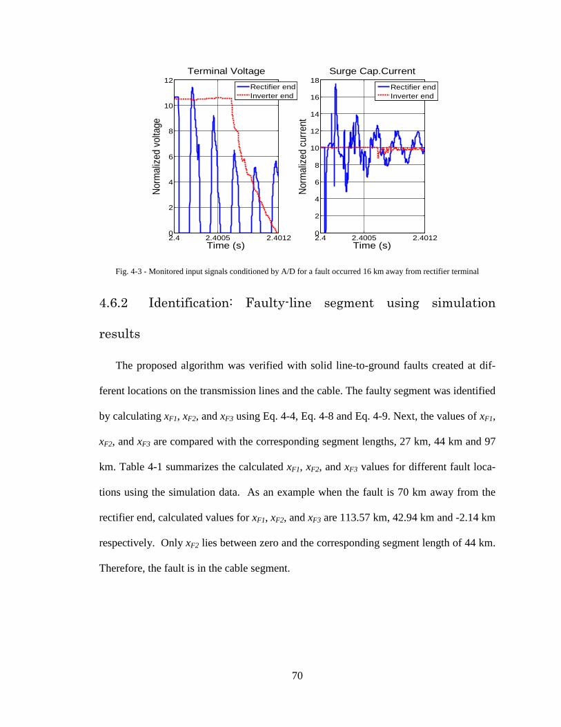
Fig. 4-3 - Monitored input signals conditioned by A/D for a fault occurred 16 km away from rectifier terminal
4.6.2 Identification: Faulty-line segment using simulation
results
The proposed algorithm was verified with solid line-to-ground faults created at dif-
ferent locations on the transmission lines and the cable. The faulty segment was identified
by calculating xF1, xF2, and xF3 using Eq. 4-4, Eq. 4-8 and Eq. 4-9. Next, the values of xF1,
xF2, and xF3 are compared with the corresponding segment lengths, 27 km, 44 km and 97
km. Table 4-1 summarizes the calculated xF1, xF2, and xF3 values for different fault loca-
tions using the simulation data. As an example when the fault is 70 km away from the
rectifier end, calculated values for xF1, xF2, and xF3 are 113.57 km, 42.94 km and -2.14 km
respectively. Only xF2 lies between zero and the corresponding segment length of 44 km.
Therefore, the fault is in the cable segment.
2.4 2.4005 2.40120
2
4
6
8
10
12Terminal Voltage
Time (s)
Norm
alize
d vo
ltage
Rectifier endInverter end
2.4 2.4005 2.40120
2
4
6
8
10
12
14
16
18Surge Cap.Current
Time (s)
Norm
alize
d cu
rrent
Rectifier endInverter end
70

Table 4-1 - Calculated values of xF1, xF2, and xF3 for different fault locations
4.6.3 Fault-location results
Fault-location error calculated using Eq. 4-17 was used as a performance index.
% 𝑒𝑟𝑟𝑜𝑟 =|𝑒𝑠𝑡𝑖𝑚𝑎𝑡𝑒𝑑 𝑓𝑎𝑢𝑙𝑡 𝑙𝑜𝑐𝑎𝑡𝑖𝑜𝑛 − 𝑎𝑐𝑡𝑢𝑎𝑙 𝑓𝑎𝑢𝑙𝑡 𝑙𝑜𝑐𝑎𝑡𝑖𝑜𝑛|
𝑇𝑜𝑡𝑎𝑙 𝑙𝑒𝑛𝑔𝑡ℎ 𝑜𝑓 𝑡ℎ𝑒 𝐻𝑉𝐷𝐶 𝑙𝑖𝑛𝑒 Eq. 4-17
Table 4-2 summarizes the fault-location results obtained with terminal voltage as the in-
put. The first two faults are in the first OH line, the second two faults are in the cable, and
the last two faults are the second OH line segment. Fault locations were calculated using
CWT coefficients of different scales. The best results were obtained with scale-32, with a
maximum error of 0.06% or 0.11 km. The highest error of 0.22% was observed with
scale-128.
Fault location (km)
5 26 49 70 91 167
0 ≤ xF1 ≤ 27 5.07 25.97 71.26 113.57 135.51 211.22
0 ≤ xF2 ≤ 44 -10.88 -0.51 21.95 42.94 53.82 91.38
0 ≤ xF3 ≤ 97 -111.14 -90.15 -44.65 -2.14 19.89 95.94
71
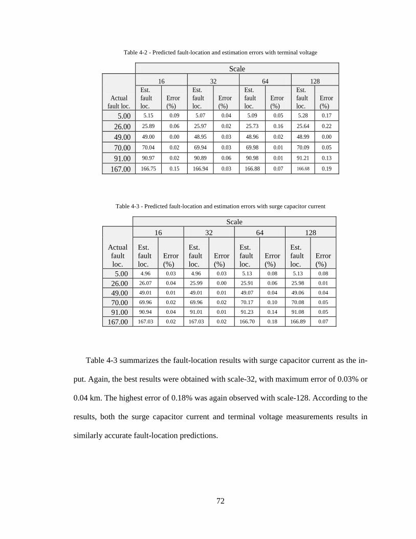
Table 4-2 - Predicted fault-location and estimation errors with terminal voltage
Table 4-3 - Predicted fault-location and estimation errors with surge capacitor current
Table 4-3 summarizes the fault-location results with surge capacitor current as the in-
put. Again, the best results were obtained with scale-32, with maximum error of 0.03% or
0.04 km. The highest error of 0.18% was again observed with scale-128. According to the
results, both the surge capacitor current and terminal voltage measurements results in
similarly accurate fault-location predictions.
Scale
Actual fault loc.
16 32 64 128 Est. fault loc.
Error (%)
Est. fault loc.
Error (%)
Est. fault loc.
Error (%)
Est. fault loc.
Error (%)
5.00 5.15 0.09 5.07 0.04 5.09 0.05 5.28 0.17
26.00 25.89 0.06 25.97 0.02 25.73 0.16 25.64 0.22
49.00 49.00 0.00 48.95 0.03 48.96 0.02 48.99 0.00
70.00 70.04 0.02 69.94 0.03 69.98 0.01 70.09 0.05
91.00 90.97 0.02 90.89 0.06 90.98 0.01 91.21 0.13
167.00 166.75 0.15 166.94 0.03 166.88 0.07 166.68 0.19
Scale
Actual fault loc.
16 32 64 128
Est. fault loc.
Error (%)
Est. fault loc.
Error (%)
Est. fault loc.
Error (%)
Est. fault loc.
Error (%)
5.00 4.96 0.03 4.96 0.03 5.13 0.08 5.13 0.08
26.00 26.07 0.04 25.99 0.00 25.91 0.06 25.98 0.01
49.00 49.01 0.01 49.01 0.01 49.07 0.04 49.06 0.04
70.00 69.96 0.02 69.96 0.02 70.17 0.10 70.08 0.05
91.00 90.94 0.04 91.01 0.01 91.23 0.14 91.08 0.05
167.00 167.03 0.02 167.03 0.02 166.70 0.18 166.89 0.07
72

4.7 Fault-location with noisy inputs
In order to examine the robustness of the proposed fault-location algorithm, fault-
location performance was tested with input signals contaminated with noise. As an ex-
ample, Fig. 4-4 shows rectifier terminal voltage and surge capacitor current contaminated
with noise. In Fig. 4-4 (a), rectifier end voltage with added 0.001 pu white noise is com-
pared with the clean signal. In Fig. 4-4 (b), the same signal with 0.01 pu white noise is
shown. Fig. 4-4 (c) and (d) compare the rectifier end surge capacitor current with 0.001
kA and 0.01 kA noise respectively with the clean signal.
Fig. 4-4 - Surge capacitor current and terminal voltage with added white noise
Results of the fault-location algorithm using the terminal voltages contaminated with
0.001 pu of noise are listed in Table 4-4. Table 4-5 shows the corresponding results with
0.01 pu noise. Although the accuracy decreases with the noise level, it is possible to lo-
cate the faults with satisfactory accuracy, even with noisy inputs. The best results are ob-
1.06321.06341.06361.06381.064
1.06421.0644
Time(s)- (a)
Rec
. ter
. vol
t (pu
)
Noisy signalOriginal signal
1.05
1.06
1.07
Time(s) - (b)
Rec
. ter
. vol
t (pu
)
Noisy signalOriginal signal
-5
0
5
10
15x 10
-4
Time(s) - (c)
Rec
.Sur
.cap
.cur
(kA
)
Noisy signalOriginal signal
-0.01
0
0.01
Time(s) - (d)
Rec
.Sur
.cap
.cur
(kA
)
Noisy signalOriginal signal
73
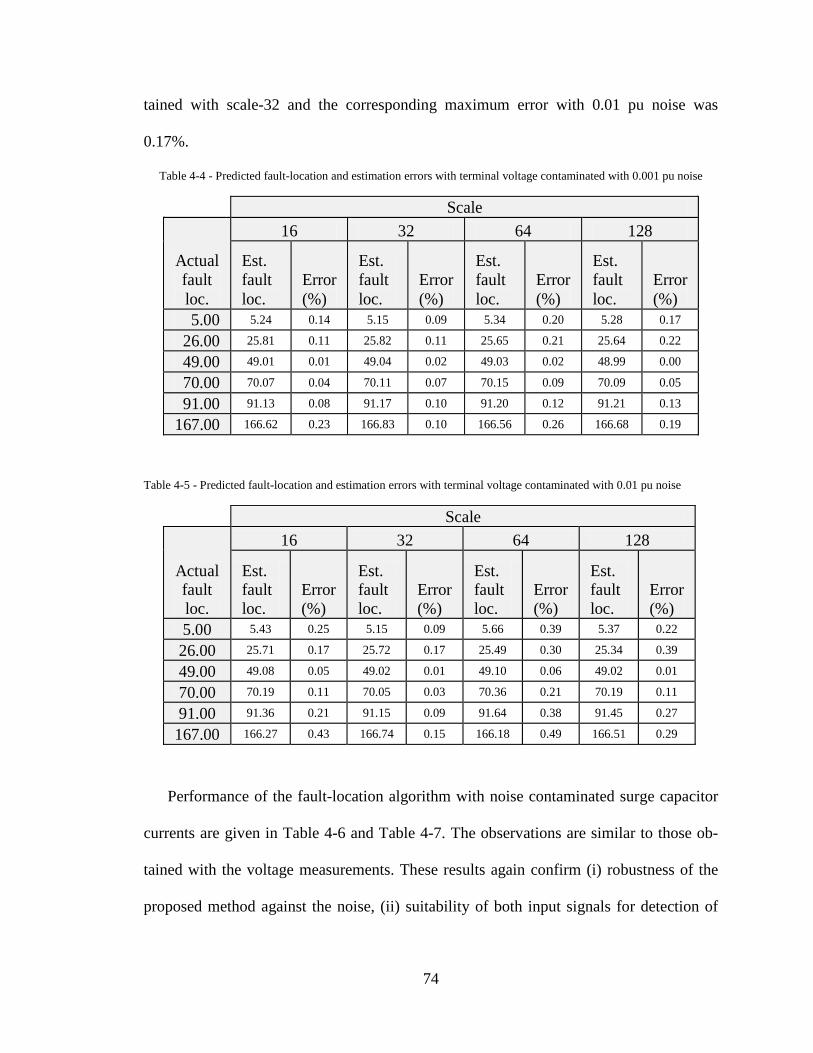
tained with scale-32 and the corresponding maximum error with 0.01 pu noise was
0.17%.
Table 4-4 - Predicted fault-location and estimation errors with terminal voltage contaminated with 0.001 pu noise
Table 4-5 - Predicted fault-location and estimation errors with terminal voltage contaminated with 0.01 pu noise
Performance of the fault-location algorithm with noise contaminated surge capacitor
currents are given in Table 4-6 and Table 4-7. The observations are similar to those ob-
tained with the voltage measurements. These results again confirm (i) robustness of the
proposed method against the noise, (ii) suitability of both input signals for detection of
Scale
Actual fault loc.
16 32 64 128
Est. fault loc.
Error (%)
Est. fault loc.
Error (%)
Est. fault loc.
Error (%)
Est. fault loc.
Error (%)
5.00 5.24 0.14 5.15 0.09 5.34 0.20 5.28 0.17
26.00 25.81 0.11 25.82 0.11 25.65 0.21 25.64 0.22
49.00 49.01 0.01 49.04 0.02 49.03 0.02 48.99 0.00
70.00 70.07 0.04 70.11 0.07 70.15 0.09 70.09 0.05
91.00 91.13 0.08 91.17 0.10 91.20 0.12 91.21 0.13
167.00 166.62 0.23 166.83 0.10 166.56 0.26 166.68 0.19
Scale
Actual fault loc.
16 32 64 128
Est. fault loc.
Error (%)
Est. fault loc.
Error (%)
Est. fault loc.
Error (%)
Est. fault loc.
Error (%)
5.00 5.43 0.25 5.15 0.09 5.66 0.39 5.37 0.22
26.00 25.71 0.17 25.72 0.17 25.49 0.30 25.34 0.39
49.00 49.08 0.05 49.02 0.01 49.10 0.06 49.02 0.01
70.00 70.19 0.11 70.05 0.03 70.36 0.21 70.19 0.11
91.00 91.36 0.21 91.15 0.09 91.64 0.38 91.45 0.27
167.00 166.27 0.43 166.74 0.15 166.18 0.49 166.51 0.29
74
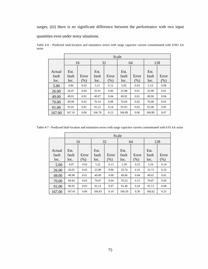
surges, (iii) there is no significant difference between the performance with two input
quantities even under noisy situations.
Table 4-6 - Predicted fault-location and estimation errors with surge capacitor current contaminated with 0.001 kA noise
Table 4-7 - Predicted fault-location and estimation errors with surge capacitor current contaminated with 0.01 kA noise
Scale
Actual fault loc.
16 32 64 128
Est. fault loc.
Error (%)
Est. fault loc.
Error (%)
Est. fault loc.
Error (%)
Est. fault loc.
Error (%)
5.00 4.96 0.03 5.21 0.12 5.05 0.03 5.13 0.08
26.00 26.07 0.04 25.91 0.06 25.98 0.01 25.98 0.01
49.00 49.01 0.01 49.07 0.04 49.02 0.01 49.06 0.04
70.00 69.96 0.02 70.14 0.08 70.04 0.02 70.08 0.05
91.00 91.01 0.01 91.23 0.14 91.03 0.02 91.08 0.05
167.00 167.10 0.06 166.78 0.13 166.89 0.06 166.89 0.07
Scale
Actual fault loc.
16 32 64 128
Est. fault loc.
Error (%)
Est. fault loc.
Error (%)
Est. fault loc.
Error (%)
Est. fault loc.
Error (%)
5.00 4.97 0.02 5.22 0.13 5.39 0.23 5.24 0.14
26.00 26.05 0.03 25.89 0.06 25.74 0.16 25.73 0.16
49.00 48.98 0.01 49.00 0.00 49.06 0.04 49.01 0.01
70.00 69.94 0.03 70.07 0.04 70.25 0.15 70.07 0.04
91.00 90.95 0.03 91.12 0.07 91.40 0.24 91.13 0.08
167.00 167.01 0.00 166.83 0.10 166.50 0.30 166.62 0.23
75
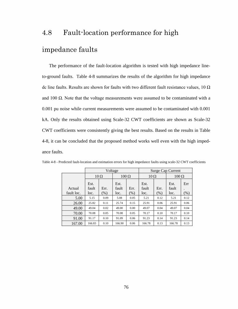
4.8 Fault-location performance for high
impedance faults
The performance of the fault-location algorithm is tested with high impedance line-
to-ground faults. Table 4-8 summarizes the results of the algorithm for high impedance
dc line faults. Results are shown for faults with two different fault resistance values, 10 Ω
and 100 Ω. Note that the voltage measurements were assumed to be contaminated with a
0.001 pu noise while current measurements were assumed to be contaminated with 0.001
kA. Only the results obtained using Scale-32 CWT coefficients are shown as Scale-32
CWT coefficients were consistently giving the best results. Based on the results in Table
4-8, it can be concluded that the proposed method works well even with the high imped-
ance faults.
Table 4-8 - Predicted fault-location and estimation errors for high impedance faults using scale-32 CWT coefficients
Voltage Surge Cap Current
Actual fault loc.
10 Ω 100 Ω 10 Ω 100 Ω
Est. fault loc.
Err. (%)
Est. fault loc.
Err. (%)
Est. fault loc.
Err. (%)
Est. fault loc.
Err. (%)
5.00 5.15 0.09 5.08 0.05 5.21 0.12 5.21 0.12
26.00 25.82 0.11 25.74 0.15 25.91 0.06 25.91 0.06
49.00 49.04 0.02 49.00 0.00 49.07 0.04 49.07 0.04
70.00 70.08 0.05 70.08 0.05 70.17 0.10 70.17 0.10
91.00 91.17 0.10 91.09 0.06 91.23 0.14 91.23 0.14
167.00 166.83 0.10 166.90 0.06 166.78 0.13 166.78 0.13
76

4.9 Theoretical extension of the algorithm to an 'n'-
segment HVDC transmission system
Fig. 4-5 - HVDC system with “n” number of line segments where fault is in ith segment
Fig. 4-5 illustrates an HVDC scheme with “n” different transmission segments which
have segment lengths of L1, L2, .., Ln-1, Ln and propagation velocities of v1, v2, .., vn-1, vn.
In order to derive an expression for the fault-location in this general case, consider a case
where a fault in Segment “i”.
If xFi is calculated in terms of the surge-arrival time difference for the fault Fi
𝑥𝐹𝑖 = ∆𝑡12−𝐹𝑖 −𝐿1𝑣1−𝐿2𝑣2− ⋯−
𝐿𝑥−1𝑣𝑥−1
−𝐿𝑥𝑣𝑥−𝐿𝑥+1𝑣𝑥+1
…−𝐿𝑖−1𝑣𝑖−1
+𝐿𝑖𝑣𝑖
+𝐿𝑖+1𝑣𝑖+1
. . . +𝐿𝑦−1𝑣𝑦−1
+𝐿𝑦𝑣𝑦
+𝐿𝑦+1𝑣𝑦+1
… +𝐿𝑛𝑣𝑛 ×
𝑣𝑖2
Eq. 4-18
Since the actual fault-location is initially unknown and only the surge-arrival time differ-
ence is available; one may assume the fault is in segment “x” and calculate the fault-
location xFx using the surge-arrival time difference as,
𝑥𝐹𝑥 = ∆𝑡12−𝐹𝑖 −𝐿1𝑣1−𝐿2𝑣2− ⋯−
𝐿𝑥−1𝑣𝑥−1
+𝐿𝑥𝑣𝑥
+𝐿𝑥+1𝑣𝑥+1
… +𝐿𝑖−1𝑣𝑖−1
+𝐿𝑖𝑣𝑖
+𝐿𝑖+1𝑣𝑖+1
. . . +𝐿𝑦−1𝑣𝑦−1
+𝐿𝑦𝑣𝑦
+𝐿𝑦+1𝑣𝑦+1
… +𝐿𝑛𝑣𝑛 ×
𝑣𝑥2
Eq. 4-19
Rectifier end
Inverter end
1 2 (n-1) nT1 T2
v1 v2 v(n-1)vn
xF(x)
xvx
x+1vx+1
x-1vx-1
xF(i)
iviFi
i+1vi+1
i-1vi-1
xF(y)
yvy
y+1vy+1
y-1vy-1
77

If xFx rewrites in terms of xFi, (actual fault-location)
𝑥𝐹𝑥 = 2𝑥𝐹𝑖𝑣𝑖
+ 𝐿𝑥𝑣𝑥
+𝐿𝑥+1𝑣𝑥+1
… +𝐿𝑖−1𝑣𝑖−1
− 𝐿𝑖𝑣𝑖
+𝐿𝑖+1𝑣𝑖+1
. . . +𝐿𝑦−1𝑣𝑦−1
+𝐿𝑦𝑣𝑦
+𝐿𝑦+1𝑣𝑦+1
… +𝐿𝑛𝑣𝑛 +
𝐿𝑥𝑣𝑥
+𝐿𝑥+1𝑣𝑥+1
…
+𝐿𝑖−1𝑣𝑖−1
+𝐿𝑖𝑣𝑖
+𝐿𝑖+1𝑣𝑖+1
. . . +𝐿𝑦−1𝑣𝑦−1
+𝐿𝑦𝑣𝑦
+𝐿𝑦+1𝑣𝑦+1
… +𝐿𝑛𝑣𝑛 ×
𝑣𝑥2
Eq. 4-20
𝑥𝐹𝑥 = 2𝑥𝐹𝑖𝑣𝑖
+ 2 𝐿𝑥𝑣𝑥
+𝐿𝑥+1𝑣𝑥+1
… +𝐿𝑖−1𝑣𝑖−1
×𝑣𝑥2
𝑥𝐹𝑥 = 𝐿𝑥 + 2𝑥𝐹𝑖𝑣𝑖
+ 2 𝐿𝑥+1𝑣𝑥+1
… +𝐿𝑖−1𝑣𝑖−1
×𝑣𝑥2
≥0
𝑥𝐹𝑥 ≥ 𝐿𝑥 Eq. 4-21
Similarly, one could assume the fault is in segment “y” and calculate the fault-location xFy
using the surge-arrival time difference as,
𝑥𝐹𝑦 = ∆𝑡12−𝐹𝑖 −𝐿1𝑣1−𝐿2𝑣2− ⋯−
𝐿𝑥−1𝑣𝑥−1
−𝐿𝑥𝑣𝑥−𝐿𝑥+1𝑣𝑥+1
…−𝐿𝑖−1𝑣𝑖−1
−𝐿𝑖𝑣𝑖
−𝐿𝑖+1𝑣𝑖+1
. . .−𝐿𝑦−1𝑣𝑦−1
+𝐿𝑦𝑣𝑦
+𝐿𝑦+1𝑣𝑦+1
… +𝐿𝑛𝑣𝑛 ×
𝑣𝑦2
Eq. 4-22
78

𝑥𝐹𝑦 = 2𝑥𝐹𝑖𝑣𝑖
− 𝐿𝑖𝑣𝑖
+𝐿𝑖+1𝑣𝑖+1
+ ⋯+𝐿𝑦−1𝑣𝑦−1
+𝐿𝑦𝑣𝑦
+𝐿𝑦+1𝑣𝑦+1
… +𝐿𝑛𝑣𝑛 −
𝐿𝑖𝑣𝑖−𝐿𝑖+1𝑣𝑖+1
…
−𝐿𝑦−1𝑣𝑦−1
+𝐿𝑦𝑣𝑦
+𝐿𝑦+1𝑣𝑦+1
… +𝐿𝑛𝑣𝑛 ×
𝑣𝑦2
𝑥𝐹𝑦 = 2𝑥𝐹𝑖𝑣𝑖
− 2 𝐿𝑖𝑣𝑖
+𝐿𝑖+1𝑣𝑖+1
… +𝐿𝑦−1𝑣𝑦−1
+𝐿𝑦𝑣𝑦
+𝐿𝑦+1𝑣𝑦+1
+ ⋯+𝐿𝑛𝑣𝑛 ×
𝑣𝑦2
𝑥𝐹𝑥 = 𝑥𝐹𝑖 − 𝐿𝑖𝑣𝑖≤0
− 𝐿𝑖+1𝑣𝑖+1
… +𝐿𝑦−1𝑣𝑦−1
+𝐿𝑦𝑣𝑦
+𝐿𝑦+1𝑣𝑦+1
+ ⋯+𝐿𝑛𝑣𝑛 × 𝑣𝑦
𝑥𝐹𝑥 ≤ 0 Eq. 4-23
Therefore, Eq. 4-21 and Eq. 4-23 show the calculated fault locations are not within the
respective line length. In this case, only xFi should lie between ‘zero’ and Li. Therefore,
this method can be extended for an HVDC system with n-number of segments. All other
possibilities (xF1, xF2, … xFi-1, xFi+1, … xFn) calculated using the corresponding time dif-
ference, Δt12-Fi, will lie outside their valid ranges.
4.10 Concluding remarks
An algorithm to locate faults on an HVDC transmission system consisting of seg-
ments of cables and overhead lines using only the terminal measurements was proposed
in this Chapter. The proposed algorithm that uses the two-terminal travelling-wave fault-
location principle has the ability to correctly identify the faulted line segment using only
the measurements at two ends.
79

Application of the proposed fault-location method to an HVDC system consisting of
two overhead line segments and one cable segment was demonstrated through simula-
tions. The simulation results verified the correct operation of the fault-location algorithm.
According to the simulation results, it is possible to achieve a fault-location accuracy of ±
400 m for the test system considered. Further simulations showed that the proposed
method performs well under the presence of measurement noise even for the high imped-
ance faults. The analysis, which considered the scaling and quantization effects of the
A/D conversion, indicated that either the terminal voltage or the surge capacitor current
could be used as the input signal, and in both cases, Scale-32 CWT coefficients (calcu-
lated at 2 MHz sampling rate) are the best for detecting surge-arrival time.
The proposed method eliminates the need for the installation of LFL detection sta-
tions at the ends of each OH line section, and provides an indication of the location of the
fault even when it is inside the cable section. Although the method is described using a
three section HVDC transmission system, it can be generalized to an n-section HVDC
transmission system.
80

Chapter 5
Fault-location in star-connected multi-
terminal HVDC schemes
5.1 Introduction
Multi-terminal HVDC (MTHVDC) technology based on voltage-source converters
(VSC) is expected to be widely used for the interconnection of on-shore wind farms like
the Atlantic wind connection [35], as well as in underground urban sub-transmission sys-
tems as proposed in [36], and off shore renewable generation systems as discussed in [5]
and [37]. Multi-terminal HVDC systems which have more than two converters connected
to a common HVDC system can have different topologies such as point to point, general
ring and star topologies [5][37].
When a line fault occurs in a multi-terminal HVDC scheme, the primary protection
must activate and isolate the faulted line segment. Several methods to identify the faulty
line in a multi-terminal VSC HVDC network with mesh topology are proposed in [5] and
[19]. These methods, which are based on the current and voltage measurements at the
converter terminals, have been primarily developed for protection purposes. However, in
case of a permanent dc line fault, determination of the exact fault-location is essential for
81

carrying out the repairs. If this can be achieved without any additional tests, repair crews
can be dispatched immediately ensuring faster network restoration.
Consider a star network topology, where the fault-location can be achieved by using
the existing two-terminal travelling-wave based fault locators with synchronized meas-
urements, if fault locators are placed at all the terminals and at the common point. How-
ever, installing a fault locator at the star point requires additional equipment as well as
communication infrastructure, and therefore incurs additional costs.
Several algorithms based on the travelling-wave principle have been proposed for
fault-location in ac transmission networks [38] - [45]. The ‘teed’ circuit-protection algo-
rithms proposed in [38] and [40] relies on the secondary reflections to locate the faulty
line. Therefore, the accuracy of the fault-location can be degraded due to multiple and
superimposed reflections and refractions of travelling waves, although such algorithms
are advantageous when synchronized measurements are not available. In those algo-
rithms, wave fronts are identified using auto and cross correlation. The benefits of apply-
ing wavelet transform to identify the wave front arrival time were explained in chapter 2
and 3. In ac transmission systems, post fault voltages and currents of the line within the
first 5ms are used to find the fault-location in [41]. This may not be feasible in HVDC
systems, due to the presence of fast acting protection. In [42] and [43], discrete wavelet
transform is used to identify the wave front arrival time and Dijkstra’s shortest path algo-
rithm is adapted to identify the fault-location. The advantage of using continuous wavelet
transform over discrete wavelet transform to identify the wave-front arrival time is dis-
cussed in Chapter 2. The method proposed to use in ac network fault-location in [45] also
82
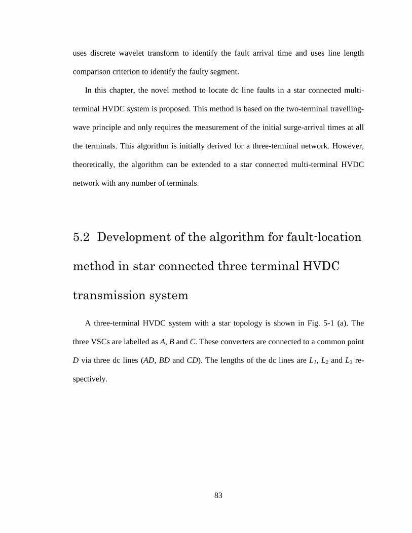
uses discrete wavelet transform to identify the fault arrival time and uses line length
comparison criterion to identify the faulty segment.
In this chapter, the novel method to locate dc line faults in a star connected multi-
terminal HVDC system is proposed. This method is based on the two-terminal travelling-
wave principle and only requires the measurement of the initial surge-arrival times at all
the terminals. This algorithm is initially derived for a three-terminal network. However,
theoretically, the algorithm can be extended to a star connected multi-terminal HVDC
network with any number of terminals.
5.2 Development of the algorithm for fault-location
method in star connected three terminal HVDC
transmission system
A three-terminal HVDC system with a star topology is shown in Fig. 5-1 (a). The
three VSCs are labelled as A, B and C. These converters are connected to a common point
D via three dc lines (AD, BD and CD). The lengths of the dc lines are L1, L2 and L3 re-
spectively.
83

Fig. 5-1 - (a) Star connected three-terminal HVDC system (b) dc line fault F1 inside line AD
An arbitrary dc line fault is shown in Fig. 5-1(b). The distance to the fault is calculat-
ed from each converter terminal. For example, xA-F1, xB-F1 and xC-F1 are the distances to
fault F1 from terminals A, B and C respectively. Assume that the fault occurs at time t=0,
and that the time of arrival of the initial travelling-wave at terminals A, B and C are given
by tA-F1, tB-F1 and tC-F1 respectively. Each of these travel times can be expressed in terms
of the dc transmission line lengths and xA-F1 as follows:
𝑡𝐴−𝐹1 = 𝑥𝐴−𝐹1𝑣1
Eq. 5-1
𝑡𝐵−𝐹1 = 𝐿1 − 𝑥𝐴−𝐹1
𝑣1 +
𝐿2𝑣2 Eq. 5-2
𝑡𝐶−𝐹1 = 𝐿1 − 𝑥𝐴−𝐹1
𝑣1 +
𝐿3𝑣3 Eq. 5-3
Where v1, v2 and v3 are the travelling-wave propagation velocities of the dc transmis-
sion line sections AD, BD and CD respectively. In obtaining Eq. 5-1 to Eq. 5-3, it is as-
L1
L2
L3
A
B
C
(a)
D
xB-F1
A
B
C
tA-F1
xA-F1
xC-F1
(b)
F1
tB-F1
tC-F1D
84

sumed that the fault is inside the AD line. By subtracting Eq. 5-2 from Eq. 5-1, we can
obtain an expression for the difference between surge-arrival times at terminals A and B:
∆𝑡𝐴𝐵−𝐹1 = 𝑡𝐴−𝐹1 − 𝑡𝐵−𝐹1 =2 ∙ 𝑥𝐴−𝐹1
𝑣1−𝐿1𝑣1−𝐿2𝑣2
Eq. 5-4
Similarly, by subtracting Eq. 5-3 from Eq. 5-1, the difference between surge-arrival
times at terminals A and C can be obtained as:
∆𝑡𝐴𝐶−𝐹1 = 𝑡𝐴−𝐹1 − 𝑡𝐶−𝐹1 =2 ∙ 𝑥𝐴−𝐹1
𝑣1−𝐿1𝑣1−𝐿3𝑣3
Eq. 5-5
Two estimations for the distance to the fault from terminal A can be obtained in terms
of ΔtAB-F1 and ΔtAC-F1.
𝑥𝐴−𝐹1 = ∆𝑡𝐴𝐵−𝐹1 +𝐿1𝑣1
+𝐿2𝑣2 ×
𝑣12
Eq. 5-6
𝑥𝐴−𝐹1 = ∆𝑡𝐴𝐶−𝐹1 +𝐿1𝑣1
+𝐿3𝑣3 ×
𝑣12
Eq. 5-7
If ΔtAB-F1 and ΔtAC-F1 can be obtained through GPS based measurements, then the fault
can be located with known propagation velocities. Note that the values of ΔtAB-F1 and
ΔtAC-F1 can be negative depending on the line lengths and the fault-location. Regardless,
the distance to the fault from terminal 'A' will always be correctly given if the time differ-
ences are computed as in Eq. 5-4 and Eq. 5-5.
In the above case the fault was inside the dc line Section AD. Now consider fault F2
which is in the line Section BD as indicated on Fig. 5-2 (a). Again, assume that the fault
occurs at the instant t=0.
85
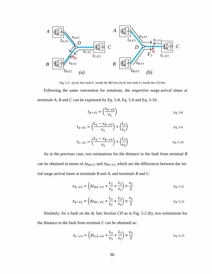
Fig. 5-2 - (a) dc line fault F2 inside the BD line (b) dc line fault F3 inside the CD line
Following the same convention for notations, the respective surge-arrival times at
terminals A, B and C can be expressed by Eq. 5-8, Eq. 5-9 and Eq. 5-10.
𝑡𝐵−𝐹2 = 𝑥𝐵−𝐹2𝑣2
Eq. 5-8
𝑡𝐴−𝐹2 = 𝐿2 − 𝑥𝐵−𝐹2
𝑣2 +
𝐿1𝑣1 Eq. 5-9
𝑡𝐶−𝐹2 = 𝐿2 − 𝑥𝐵−𝐹2
𝑣2 +
𝐿3𝑣3 Eq. 5-10
As in the previous case, two estimations for the distance to the fault from terminal B
can be obtained in terms of ∆tBA-F2 and ∆tBC-F2, which are the differences between the ini-
tial surge-arrival times at terminals B and A, and terminals B and C.
𝑥𝐵−𝐹2 = ∆𝑡𝐵𝐴−𝐹2 +𝐿2𝑣2
+𝐿1𝑣1 ×
𝑣22
Eq. 5-11
𝑥𝐵−𝐹2 = ∆𝑡𝐵𝐶−𝐹2 +𝐿2𝑣2
+𝐿3𝑣3 ×
𝑣22
Eq. 5-12
Similarly, for a fault on the dc line Section CD as in Fig. 5-2 (b), two estimations for
the distance to the fault from terminal C can be obtained as:
𝑥𝐶−𝐹3 = ∆𝑡𝐶𝐴−𝐹3 +𝐿3𝑣3
+𝐿1𝑣1 ×
𝑣32
Eq. 5-13
xB-F2
A
B
CtA-F2
tB-F2
tC-F2
xA-F2
xC-F2
D
(a)
xB-F3
A
B
CtA-F3
tB-F3
tC-F3
xA-F3 xC-F3
D
(b)
F3
86

𝑥𝐶−𝐹3 = ∆𝑡𝐶𝐵−𝐹3 +𝐿3𝑣3
+𝐿2𝑣2 ×
𝑣32
Eq. 5-14
Where ΔtCA-F3 and ΔtCB-F3 are the differences between the initial surge-arrival times at
terminals C and A, and terminals C and B respectively.
5.3 Identification: Correct faulty dc line
In deriving the expressions Eq. 5-6 - Eq. 5-7 and Eq. 5-11 - Eq. 5-14 for the distance
to a fault, it was assumed that the faulted dc line section is known. However, in a practi-
cal fault-location problem, this is unknown. The only measurable quantities are the dif-
ferences between the surge-arrival times. Thus, it is necessary to identify the faulted dc
line before being able to pinpoint the exact location of the fault. This can be achieved by
the procedure described below.
When a fault is detected, two estimations for the fault-location are calculated using
Eq. 5-6 and Eq. 5-7, assuming that the fault is inside dc line Section AD. Then two more
estimations for the fault-location are calculated using Eq. 5-11 and Eq. 5-12, assuming
that the fault is inside dc line Section BD. Finally, two more fault-location values are cal-
culated using the surge-arrival time difference measurements by using Eq. 5-13 and Eq.
5-14, assuming that the fault is inside dc line Section CD. Next, the pair of calculated
fault-location values under each assumption are compared with each other for consis-
tency. For example, if the assumption that the fault is inside the dc line Section AD is cor-
rect, then the fault distances calculated from Eq. 5-6 and Eq. 5-7 have to be the same.
Furthermore, for this fault, the fault distances calculated from Eq. 5-11 and Eq. 5-12 will
not be the same, since the underlying assumptions for Eq. 5-11 and Eq. 5-12 are not true.
87
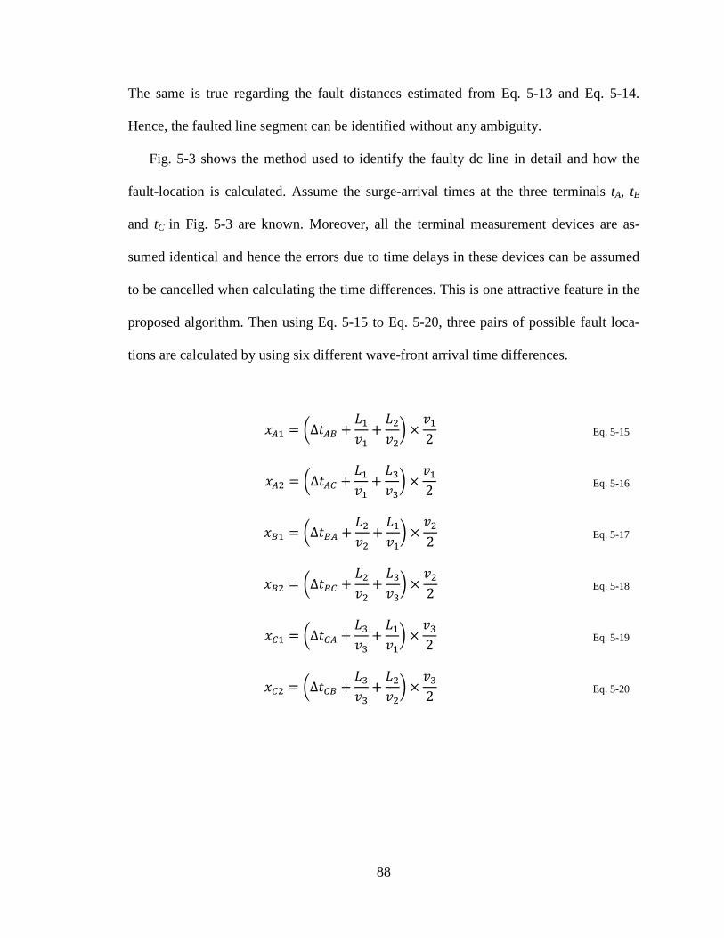
The same is true regarding the fault distances estimated from Eq. 5-13 and Eq. 5-14.
Hence, the faulted line segment can be identified without any ambiguity.
Fig. 5-3 shows the method used to identify the faulty dc line in detail and how the
fault-location is calculated. Assume the surge-arrival times at the three terminals tA, tB
and tC in Fig. 5-3 are known. Moreover, all the terminal measurement devices are as-
sumed identical and hence the errors due to time delays in these devices can be assumed
to be cancelled when calculating the time differences. This is one attractive feature in the
proposed algorithm. Then using Eq. 5-15 to Eq. 5-20, three pairs of possible fault loca-
tions are calculated by using six different wave-front arrival time differences.
𝑥𝐴1 = ∆𝑡𝐴𝐵 +𝐿1𝑣1
+𝐿2𝑣2 ×
𝑣12
Eq. 5-15
𝑥𝐴2 = ∆𝑡𝐴𝐶 +𝐿1𝑣1
+𝐿3𝑣3 ×
𝑣12
Eq. 5-16
𝑥𝐵1 = ∆𝑡𝐵𝐴 +𝐿2𝑣2
+𝐿1𝑣1 ×
𝑣22
Eq. 5-17
𝑥𝐵2 = ∆𝑡𝐵𝐶 +𝐿2𝑣2
+𝐿3𝑣3 ×
𝑣22
Eq. 5-18
𝑥𝐶1 = ∆𝑡𝐶𝐴 +𝐿3𝑣3
+𝐿1𝑣1 ×
𝑣32
Eq. 5-19
𝑥𝐶2 = ∆𝑡𝐶𝐵 +𝐿3𝑣3
+𝐿2𝑣2 ×
𝑣32
Eq. 5-20
88

Fig. 5-3 - Faulty segment identification and fault calculation method
In calculating each pair of fault locations, the assumption is that the fault is in the line
segment directly connected to the considered terminal. For example, in calculating xC1
and xC2, it is assumed that fault is in line section CD. Then the ratio between the smaller
and the larger values of the estimated fault location is calculated for each pair:
𝑅𝐴 =𝑚𝑖𝑛𝑖𝑚𝑢𝑚(|𝑥𝐴1|, |𝑥𝐴2|)𝑚𝑎𝑥𝑖𝑚𝑢𝑚(|𝑥𝐴1|, |𝑥𝐴2|)
Eq. 5-21
𝑅𝐵 =𝑚𝑖𝑛𝑖𝑚𝑢𝑚(|𝑥𝐵1|, |𝑥𝐵2|)𝑚𝑎𝑥𝑖𝑚𝑢𝑚(|𝑥𝐵1|, |𝑥𝐵2|)
Eq. 5-22
𝑅𝐶 =𝑚𝑖𝑛𝑖𝑚𝑢𝑚(|𝑥𝐶1|, |𝑥𝐶2|)𝑚𝑎𝑥𝑖𝑚𝑢𝑚(|𝑥𝐶1|, |𝑥𝐶2|)
Eq. 5-23
Calculation of XA1,XA2XB1,XB2XC1,XC2
tA tB tC
Calculation of
RA,RB,RC
Find maximumfrom RA,RB,RC
If max is RAFault is in ADXf=Avg(XA1,XA2)
If max is RBFault is in BDXf=Avg(XB1,XB2)
If max is RCFault is in CDXf=Avg(XC1,XC2)
Xf Xf Xf
89

The ratio RT (where T = A, B, or C) is equal to one when the two calculated values
are equal, that is when the underline assumption is true as pointed out above. This ratio is
less than one for the remaining two cases. However in actual situations, the ratio for the
correct pair is not exactly equal to one but a value closer to one due to numerical and
measurement errors. Therefore, the terminal with the highest RT values is considered as
the terminal closest to the fault. Then the fault-location (xf) is calculated by taking the av-
erage value of the two possible fault-location values of the corresponding selected termi-
nal as shown in Eq. 5-24.
𝑋𝑓 = 0.5(𝑋𝑇∗1 + 𝑋𝑇∗2) Eq. 5-24
5.4 Calibration of the system
The accuracy of fault-location prediction is dependent on the accuracy of the propa-
gation velocity. Even though the theoretical value for the propagation velocity can be es-
timated from the conductor geometry, the best approach is to estimate these values using
the measurements obtained during the commissioning of the line fault-location system.
A systematic method for calibrating propagation velocities of a three-terminal HVDC
system is proposed in this section. This approach requires conducting three test faults,
one on each line segment at known locations. In order to simplify the equations, substi-
tute variables λ1, λ2, and λ3 represent the inverse of the propagation velocities.
𝜆1 = 1𝑣1
, 𝜆2 = 1𝑣2
and 𝜆3 = 1𝑣3
Eq. 5-25
The measured surge-arrival time differences corresponding to the faults on segments
1, 2 and 3 respectively are given by:
90
∆𝑡𝐴𝐵−𝐹1 = 𝜆1(2𝑥𝐹1 − 𝐿1) + 𝜆2(−𝐿2) + 𝜆3(0) Eq. 5-26
∆𝑡𝐵𝐴−𝐹2 = 𝜆1(−𝐿1) + 𝜆2(2𝑥𝐹2 − 𝐿2) + 𝜆3(0) Eq. 5-27
∆𝑡𝐶𝐵−𝐹3 = 𝜆1(0) + 𝜆2(−𝐿2) + 𝜆3(2𝑥𝐹3 − 𝐿3) Eq. 5-28
This set of equations can be expressed in matrix form,
(2𝑥𝐹1 − 𝐿1) (−𝐿2) 0
(−𝐿1) (2𝑥𝐹2 − 𝐿2) 00 (−𝐿2) (2𝑥𝐹3 − 𝐿3)
𝜆1𝜆2𝜆3 =
∆𝑡𝐴𝐵−𝐹1∆𝑡𝐵𝐴−𝐹2∆𝑡𝐶𝐵−𝐹3
Eq. 5-29
Solution of Eq. 5-29 with test data (with known xFi and Δt values) yields λi values, in-
version of which give the propagation velocities. Often it is not practical to place test
faults in the middle of lines, especially if they are cables. In such situations, the test faults
can be placed at the terminals and the star point. For example, if the first fault is placed at
the terminal A, then xF1=0, and if the second fault is placed at the star point xF2=L2.
Moreover, we can use the same data obtained for the second fault as inputs in equation
Eq. 5-28 and hence xF3=L3.
5.5 Identification of the fault arrival time
According to simulations it was found that for a dc line fault on a VSC based HVDC
system, a steep wave front appears on the dc line current. Nevertheless, at the moment it
is not economical to install high bandwidth transducers to measure series dc line currents.
However, if it is measurable, dc line current can be used to detect the arrival of the wave
fronts.
91
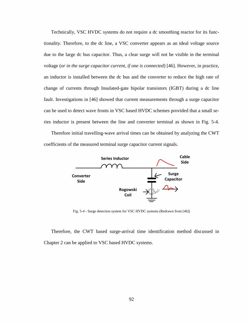
Technically, VSC HVDC systems do not require a dc smoothing reactor for its func-
tionality. Therefore, to the dc line, a VSC converter appears as an ideal voltage source
due to the large dc bus capacitor. Thus, a clear surge will not be visible in the terminal
voltage (or in the surge capacitor current, if one is connected) [46]. However, in practice,
an inductor is installed between the dc bus and the converter to reduce the high rate of
change of currents through Insulated-gate bipolar transistors (IGBT) during a dc line
fault. Investigations in [46] showed that current measurements through a surge capacitor
can be used to detect wave fronts in VSC based HVDC schemes provided that a small se-
ries inductor is present between the line and converter terminal as shown in Fig. 5-4.
Therefore initial travelling-wave arrival times can be obtained by analyzing the CWT
coefficients of the measured terminal surge capacitor current signals.
Fig. 5-4 - Surge detection system for VSC HVDC systems (Redrawn from [46])
Therefore, the CWT based surge-arrival time identification method discussed in
Chapter 2 can be applied to VSC based HVDC systems.
Series Inductor
ConverterSide
RogowskiCoil
SurgeCapacitor
Cable Side
92

5.6 Simulated case study
5.6.1 Simulation model
A star connected three-terminal VSC based HVDC system was used in simulation stud-
ies. The schematic diagram of the test network is shown in Fig. 5-5 (a). All the simula-
tions were carried out with PSCAD/EMTDC and the fault-location algorithm was im-
plemented in MATLAB.
The HVDC transmission line consists of three Over Head (OH) line segments of 27
km, 44 km and 97 km in lengths. The tower structure is shown in Fig. 5-6. OH lines are
represented using distributed parameter transmission line models in PSCAD/EMTDC.
Fig. 5-5 - (a) Test network topology & line length (b) Measured terminal dc line current
The voltage source converters are simulated using detailed models that include IGBT
switches and controllers. The ac power system connected to each converter was repre-
sented using equivalent sources.
27km
44km97km
A
B
C D
DC current measurement
VSC converter
DC line
(b)(a)
93

Fig. 5-6 - Tower structure for OH line segments
Even though current through the surge capacitor can be used to identify the surge-
arrival time as explained in section 5.5, in this chapter series line currents were used to
capture the wave front. It was found that either input would give the surge-arrival time
with equal accuracy and in the following study; it was assumed that a transducer with
high bandwidth is used to monitor the dc line currents as shown in Fig. 5-5 (b). The ac-
tual measurement scheme is not very important, as the main objective of this study is to
validate the fault-location algorithm.
Short circuit faults were applied at different locations on the dc network. Simulations
were performed in PSCAD/EMTDC with a solution time step of 0.1 µs to ensure all im-
portant high frequency components are present in the signals and the signals appear as
analog signals to the simulated signal conditioning unit. The input signals (dc line cur-
rents) were conditioned before applying to the fault-location algorithm, assuming a 2
MHz sampling rate, 16-bit A/D conversion resolution, and scaling of the current signals
to a 0-20 V range before inputting to the A/D converter. This signal conditioning allows
testing of the fault-location algorithm under the conditions similar to those existing in a
37.4
9m10
.06m
0.46m
13.41m
94

hardware implementation. The sampling frequency of 2 MHz was chosen to achieve a
high time precision, which directly imposes a limit on the theoretical accuracy.
5.6.2 Simulation results
Series dc line currents measured at terminals A, B and C are shown in Fig. 5-7(a),
when the test network was subjected to a short circuit fault in line BD, 10 km away from
terminal B. The input limits are taken as -50 kA to50 kA. It can be clearly noticed from
Fig. 5-7 (a) that the steepness and magnitude of the transients decreases as they propagate
to the A and C terminals. In Fig. 5-7(b) a zoomed view of the same signal is shown. In
this case, the fault happened 10 km away from the B terminal. Terminal surge-arrival
time differences used to calculate the fault-location are shown as ΔtAB, ΔtBC and ΔtBC.
In Fig. 5-7(c) magnitudes of the CWT coefficients of the input signals at scale 32 are
plotted. Sharp changes occur in CWT coefficients at times tA, tB and tC corresponding to
terminals A, B and C respectively. They are coincident with the wave front arrival times
at respective terminals. Multiple surges observed at terminal B are due to reflections,
since the fault is close to terminal B.
95
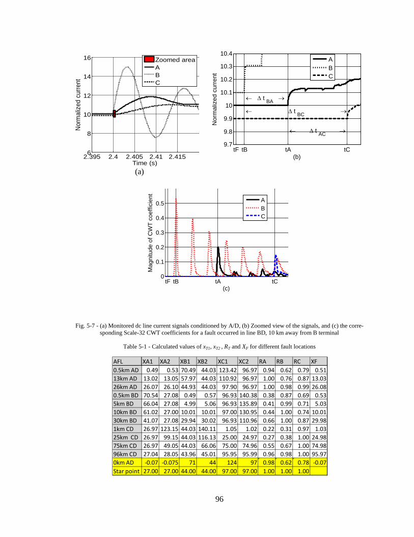
(a)
Fig. 5-7 - (a) Monitored dc line current signals conditioned by A/D, (b) Zoomed view of the signals, and (c) the corre-sponding Scale-32 CWT coefficients for a fault occurred in line BD, 10 km away from B terminal
Table 5-1 - Calculated values of xT1, xT2 , RT and XF for different fault locations
2.395 2.4 2.405 2.41 2.4156
8
10
12
14
16
Norm
alize
d cu
rrent
Time (s)
Zoomed areaABC
tF tB tA tC9.7
9.8
9.9
10
10.1
10.2
10.3
10.4
(b)
Nor
mal
ized
cur
rent
← ∆ t BC →
← ∆ t BA →
← ∆ t AC →
ABC
tF tB tA tC0
0.1
0.2
0.3
0.4
0.5
(c)
Mag
nitu
de o
f CW
T co
effic
ient
ABC
AFL XA1 XA2 XB1 XB2 XC1 XC2 RA RB RC XF0.5km AD 0.49 0.53 70.49 44.03 123.42 96.97 0.94 0.62 0.79 0.5113km AD 13.02 13.05 57.97 44.03 110.92 96.97 1.00 0.76 0.87 13.0326km AD 26.07 26.10 44.93 44.03 97.90 96.97 1.00 0.98 0.99 26.080.5km BD 70.54 27.08 0.49 0.57 96.93 140.38 0.38 0.87 0.69 0.535km BD 66.04 27.08 4.99 5.06 96.93 135.89 0.41 0.99 0.71 5.0310km BD 61.02 27.00 10.01 10.01 97.00 130.95 0.44 1.00 0.74 10.0130km BD 41.07 27.08 29.94 30.02 96.93 110.96 0.66 1.00 0.87 29.981km CD 26.97 123.15 44.03 140.11 1.05 1.02 0.22 0.31 0.97 1.0325km CD 26.97 99.15 44.03 116.13 25.00 24.97 0.27 0.38 1.00 24.9875km CD 26.97 49.05 44.03 66.06 75.00 74.96 0.55 0.67 1.00 74.9896km CD 27.04 28.05 43.96 45.01 95.95 95.99 0.96 0.98 1.00 95.970km AD -0.07 -0.075 71 44 124 97 0.98 0.62 0.78 -0.07Star point 27.00 27.00 44.00 44.00 97.00 97.00 1.00 1.00 1.00
96
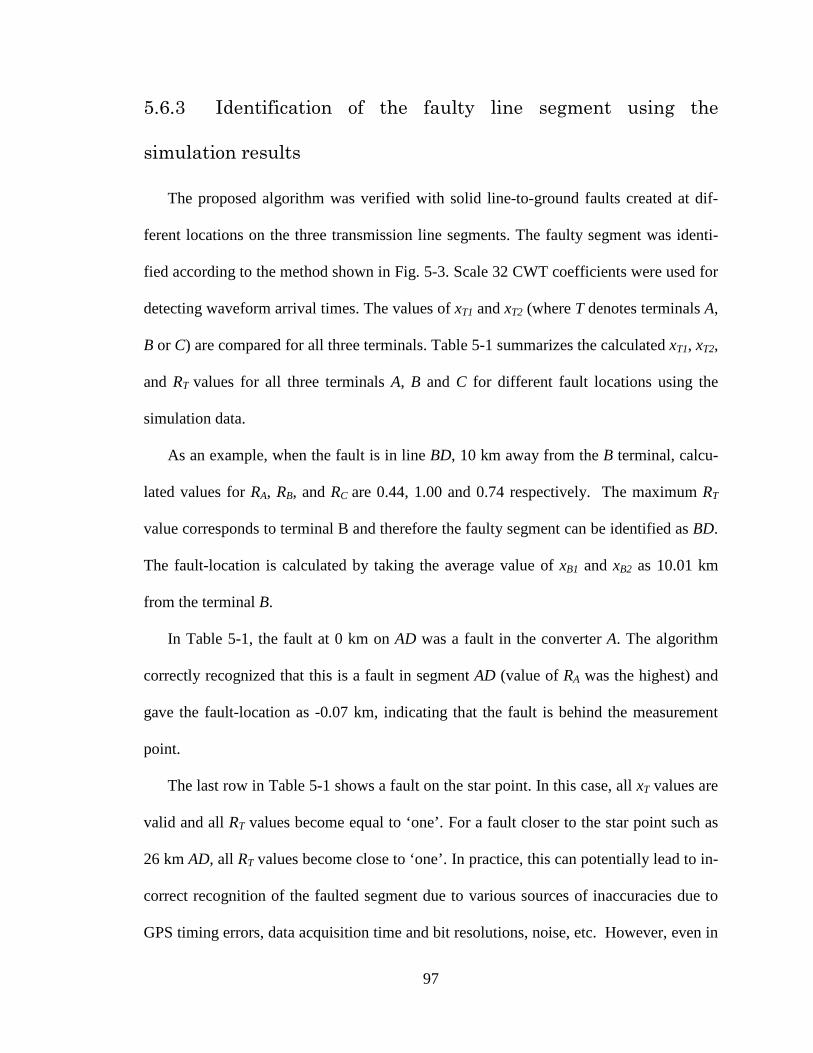
5.6.3 Identification of the faulty line segment using the
simulation results
The proposed algorithm was verified with solid line-to-ground faults created at dif-
ferent locations on the three transmission line segments. The faulty segment was identi-
fied according to the method shown in Fig. 5-3. Scale 32 CWT coefficients were used for
detecting waveform arrival times. The values of xT1 and xT2 (where T denotes terminals A,
B or C) are compared for all three terminals. Table 5-1 summarizes the calculated xT1, xT2,
and RT values for all three terminals A, B and C for different fault locations using the
simulation data.
As an example, when the fault is in line BD, 10 km away from the B terminal, calcu-
lated values for RA, RB, and RC are 0.44, 1.00 and 0.74 respectively. The maximum RT
value corresponds to terminal B and therefore the faulty segment can be identified as BD.
The fault-location is calculated by taking the average value of xB1 and xB2 as 10.01 km
from the terminal B.
In Table 5-1, the fault at 0 km on AD was a fault in the converter A. The algorithm
correctly recognized that this is a fault in segment AD (value of RA was the highest) and
gave the fault-location as -0.07 km, indicating that the fault is behind the measurement
point.
The last row in Table 5-1 shows a fault on the star point. In this case, all xT values are
valid and all RT values become equal to ‘one’. For a fault closer to the star point such as
26 km AD, all RT values become close to ‘one’. In practice, this can potentially lead to in-
correct recognition of the faulted segment due to various sources of inaccuracies due to
GPS timing errors, data acquisition time and bit resolutions, noise, etc. However, even in
97

this case, the fault-location indicated by the algorithm would be physically close to the
actual fault-location; despite it being on the wrong segment. Such erroneous recognition
of the faulted segment can be tolerated in fault-location, which is not intended for provid-
ing primary protection for the lines or bus bars.
5.7 Theoretical extension of the algorithm to star-
connected network with n-number of terminals
The fault-location method proposed in this paper can be extended to a star connected
VSC HVDC system with 'n' number of terminals.
Fig. 5-8 - N-terminal VSC HVDC system with all dc lines connect to a common point
Arbitrarily the dc line fault was placed in line section i, xi-F distance away from ter-
minal i as shown in Fig. 5-8. The distances to the fault from each terminal are denoted as,
xi-F, x2-F and xN-F which are the distances to the fault from terminals 1, 2 and N respec-
tively. If the fault occurs at time t=0, the time of arrival of the initial travelling-wave at
1
2
t1-F
v1
N
L1
i
L2
Li
LNt2-F
ti-F
tN-F
v2
vi
vN
98
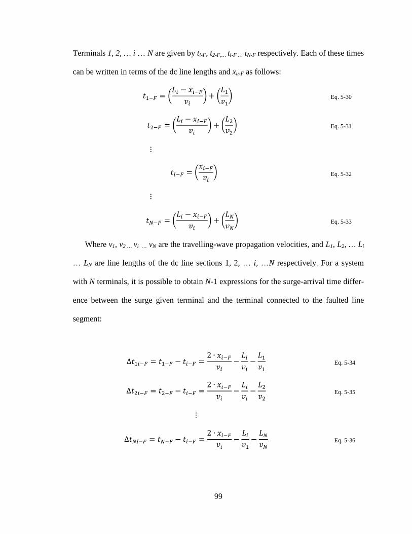
Terminals 1, 2, … i … N are given by ti-F, t2-F,… ti-F … tN-F respectively. Each of these times
can be written in terms of the dc line lengths and xu-F as follows:
𝑡1−𝐹 = 𝐿𝑖 − 𝑥𝑖−𝐹
𝑣𝑖 +
𝐿1𝑣1 Eq. 5-30
𝑡2−𝐹 = 𝐿𝑖 − 𝑥𝑖−𝐹
𝑣𝑖 +
𝐿2𝑣2 Eq. 5-31
⋮
𝑡𝑖−𝐹 = 𝑥𝑖−𝐹𝑣𝑖
Eq. 5-32
⋮
𝑡𝑁−𝐹 = 𝐿𝑖 − 𝑥𝑖−𝐹
𝑣𝑖 +
𝐿𝑁𝑣𝑁 Eq. 5-33
Where v1, v2 … vi … vN are the travelling-wave propagation velocities, and L1, L2, … Li
… LN are line lengths of the dc line sections 1, 2, … i, …N respectively. For a system
with N terminals, it is possible to obtain N-1 expressions for the surge-arrival time differ-
ence between the surge given terminal and the terminal connected to the faulted line
segment:
∆𝑡1𝑖−𝐹 = 𝑡1−𝐹 − 𝑡𝑖−𝐹 =2 ∙ 𝑥𝑖−𝐹𝑣𝑖
−𝐿𝑖𝑣𝑖−𝐿1𝑣1
Eq. 5-34
∆𝑡2𝑖−𝐹 = 𝑡2−𝐹 − 𝑡𝑖−𝐹 =2 ∙ 𝑥𝑖−𝐹𝑣𝑖
−𝐿𝑖𝑣𝑖−𝐿2𝑣2
Eq. 5-35
⋮
∆𝑡𝑁𝑖−𝐹 = 𝑡𝑁−𝐹 − 𝑡𝑖−𝐹 =2 ∙ 𝑥𝑖−𝐹𝑣𝑖
−𝐿𝑖𝑣1−𝐿𝑁𝑣𝑁
Eq. 5-36
99

Using the above equations, N-1 expressions can be obtain for the distance to the fault
from the terminal i as
𝑥𝑖−𝐹 = ∆𝑡1𝑖−𝐹 +𝐿𝑖𝑣𝑖
+𝐿1𝑣1 ×
𝑣12
Eq. 5-37
𝑥𝑖−𝐹 = ∆𝑡2𝑖−𝐹 +𝐿𝑖𝑣𝑖
+𝐿2𝑣2 ×
𝑣22
Eq. 5-38
⋮
𝑥𝑖−𝐹 = ∆𝑡𝑁𝑖−𝐹 +𝐿𝑖𝑣𝑖
+𝐿𝑁𝑣𝑁 ×
𝑣12
Eq. 5-39
If ∆t1i-F, ∆t2i-F … ∆tNi-F can be obtained through measurements then the fault can be
located with known propagation velocities and dc line segment lengths. N sets of similar
expressions can be derived by changing the faulted segment from 1 to N. Therefore for
an N line segments case, there will be N.(N-1) different equations.
Since the faulted line segment is unknown initially, possibility of the fault in any of
the N line segments is considered and for each case, (N-1) possible values for the distance
to the fault from the terminal directly connected to the considered line segment are com-
puted. If the fault is actually on the ith line segment, then all (N-1) estimated fault dis-
tances, (xi-F values) should be the same (in practice they are not exactly the same, but lie
very close to each other). Furthermore, estimated fault locations using any other equation
set will not be consistent. Hence the faulted line segment can be identified without any
ambiguity. In addition, the fault-location can be taken as the average of the (N-1) esti-
mated values for the identified faulted segment. The generalized method is shown in Fig.
5-9 which is derived from the method explained in section 5.3.
100

Fig. 5-9 - Faulty segment identification and fault calculation method for network with 'N' terminals
Generally, a simple star connected topology is not considered reliable, since any fault
in the centre node would force all converters out of service. The preferred topology is a
star connected network with a switching ring at the center. Since the fault-location calcu-
lation is based on the initial travelling-wave arrival times, the proposed method would not
be affected by the possible reflections and refractions at the ring. Typically, the length of
a switching ring would be much shorter compared to the line distances, therefore a sys-
tem with a switching ring can be effectively treated as a star connected network as far as
the fault-location is concerned.
Calculation of X1-1,X1-2X2-1,X2-2
...Xi-1,Xi-2
..XN-1,XN-2
tit2t1
Calculation of R =R1,R2,…,Ri,..RN
Where,Ri = minimum(X i-1,Xi-2) .
maximum(X i-1,Xi-2)
Find maximumOf R
If max is R1Fault is in 1S
Xf=Avg(X1-1,X1-2)
If max is R2Fault is in 2S
Xf=Avg(X2-1,X2-2)
If max is RiFault is in iS
Xf=Avg(Xi-1,Xi-2)
Xf Xf Xf
…. tN….
If max is RNFault is in NS
Xf=Avg(XN-1,XN-
2)
Xf
101
5.8 Concluding remarks
An algorithm to locate faults on star-connected multi-terminal VSC HVDC transmis-
sion lines using only the terminal measurements was proposed. The proposed algorithm
that uses the travelling-wave fault-location principle has the ability to correctly identify
the faulted line segment using only the measurements at the converter ends.
Application of the proposed fault-location method to a 3-terminal VSC HVDC system
consisting of overhead line segments was demonstrated through simulations. The simula-
tion results verified the correct operation of the fault-location algorithm. According to the
simulation results, it is possible to achieve fault-location accuracy of ± 300 m for the test
system considered using dc line currents.
The proposed method eliminates the need for the installation of repeater stations at
the junction of the multi-terminal HVDC network. Although derivations and simulations
were carried out considering a three-terminal dc network, the concept can be theoretically
expanded to an N terminal network, as shown in Section 5.7.
102

Chapter 6
Implementation and field validation of
a travelling-wave arrival-time measurement scheme
6.1 Introduction
As pointed out in the earlier chapters, the main factor that affects the accuracy of
fault-location is the accuracy of measuring the fault generated travelling-wave arrival
times. It is important to ensure that instrumentation employed for these measurements
perform properly under substation environments rich in electromagnetic noise. A number
of commercial dc line fault-location systems that use the travelling-wave principle have
been developed and some of the details have been published in literature (E.g. [20], [21]
and [47]). However, none of them has clearly explained the method of capturing the
wave-fronts arrival times. In this chapter, a method for detecting the arrival of fault tran-
sients using the surge capacitor currents is proposed. In this scheme a Rogowski coil
functions as the sensor, and its output voltage is continuously monitored using a data ac-
103

quisition (DAQ) system. A GPS clock signal is provided to the DAQ system to time syn-
chronize the measurements.
A prototype of the proposed travelling-wave arrival time measurement system was
implemented and field-tested at the Nelson River HVDC Scheme in Manitoba, Canada
[66].The practical problems such as bandwidth capability, noise level and the output volt-
age magnitudes involved in the application of a Rogowski coil as the transducer are
solved with a successful field implementation. In the following sections, the important
steps in the development of the experimental setup are described. Furthermore, the field
data gathered during the 23rd of July 2012 to the 4th of September 2012 are analysed and
compared with the existing fault locator results. However, the main objective of the ex-
perimental setup is to validate the usage of the transducer and the data acquisition system.
The experiments were not designed to compare with the existing fault locator even
though some results of the existing setup are used to validate the experimental unit.
In Chapters 2 and 3, the Continuous Wavelet Transform coefficient of the surge ca-
pacitor current measurements was used to detect the travelling-wave arrival times. How-
ever, during the field tests, it was found that the Rogowski coil sensor output voltage
could be directly used for detecting the travelling-wave arrival times with high accuracy.
Comparison of the results obtained with direct measurements to the results obtained with
the CWT based method discussed in Chapter 3 showed that both approaches result in a
similar level of accuracy.
104

6.2 Arrangement of the surge-arrival time
measurement system
Fig. 6-1 - Wave-front detection system
The simplified arrangement of the wave-front detection system is shown Fig. 6-1. The
surge capacitor is typically used in conventional HVDC converter stations to protect the
converter station equipment from surges travelling along the dc line. Additionally, the
current going through the surge capacitor can be used to capture the wave-front and this
method has been used before in [20], [21] and [47] to acquire the wave-fronts. In this ar-
rangement, the transducer is located on the ground potential and it is not directly con-
nected to the HVDC system. Therefore, the measurement system requires lower insula-
tion protection and has negligible interaction with the HVDC system. Installation of the
measuring system does not require a complete shutdown of the system and it is very easy
to mount around the ground wire because the used transducer is a clamp on type flexible
Rogowski coil.
Converterside
DC line side
Surge cap.Rogowski coil measurement
105
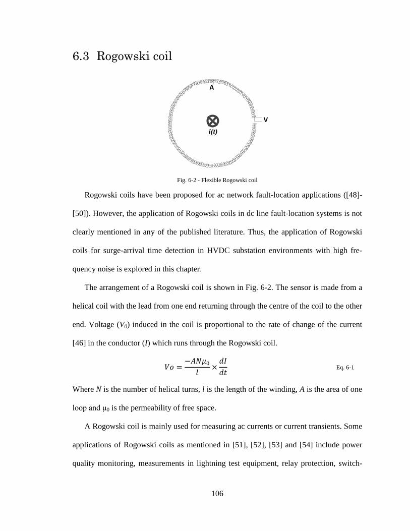
6.3 Rogowski coil
Fig. 6-2 - Flexible Rogowski coil
Rogowski coils have been proposed for ac network fault-location applications ([48]-
[50]). However, the application of Rogowski coils in dc line fault-location systems is not
clearly mentioned in any of the published literature. Thus, the application of Rogowski
coils for surge-arrival time detection in HVDC substation environments with high fre-
quency noise is explored in this chapter.
The arrangement of a Rogowski coil is shown in Fig. 6-2. The sensor is made from a
helical coil with the lead from one end returning through the centre of the coil to the other
end. Voltage (V0) induced in the coil is proportional to the rate of change of the current
[46] in the conductor (I) which runs through the Rogowski coil.
𝑉𝑜 =−𝐴𝑁𝜇0
𝑙×𝑑𝐼𝑑𝑡
Eq. 6-1
Where N is the number of helical turns, l is the length of the winding, A is the area of one
loop and μ0 is the permeability of free space.
A Rogowski coil is mainly used for measuring ac currents or current transients. Some
applications of Rogowski coils as mentioned in [51], [52], [53] and [54] include power
quality monitoring, measurements in lightning test equipment, relay protection, switch-
A
V
i(t)
106
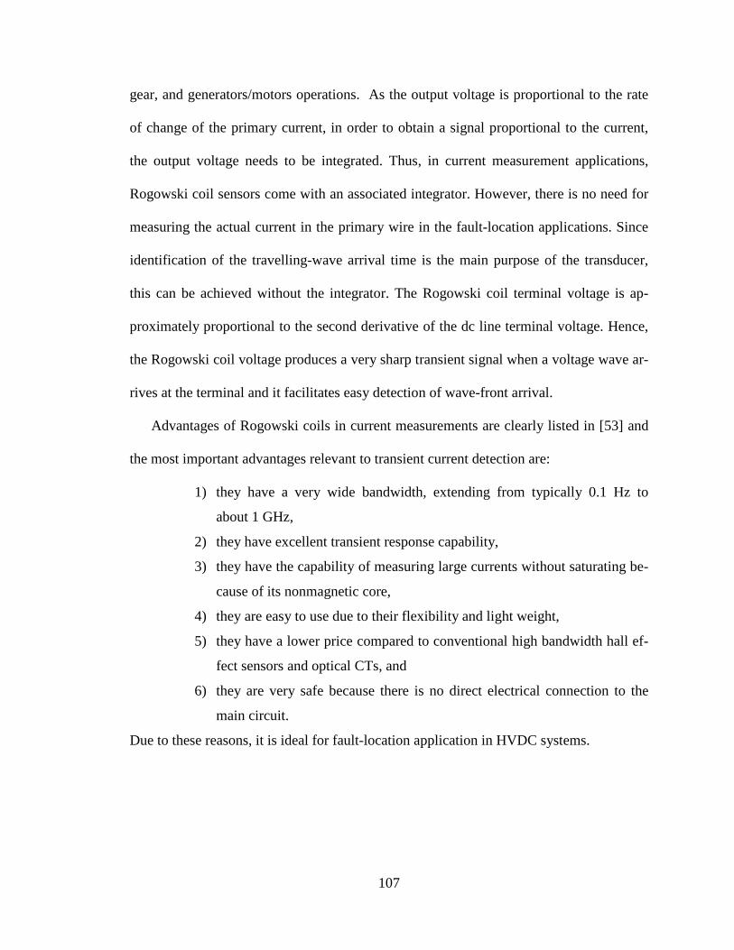
gear, and generators/motors operations. As the output voltage is proportional to the rate
of change of the primary current, in order to obtain a signal proportional to the current,
the output voltage needs to be integrated. Thus, in current measurement applications,
Rogowski coil sensors come with an associated integrator. However, there is no need for
measuring the actual current in the primary wire in the fault-location applications. Since
identification of the travelling-wave arrival time is the main purpose of the transducer,
this can be achieved without the integrator. The Rogowski coil terminal voltage is ap-
proximately proportional to the second derivative of the dc line terminal voltage. Hence,
the Rogowski coil voltage produces a very sharp transient signal when a voltage wave ar-
rives at the terminal and it facilitates easy detection of wave-front arrival.
Advantages of Rogowski coils in current measurements are clearly listed in [53] and
the most important advantages relevant to transient current detection are:
1) they have a very wide bandwidth, extending from typically 0.1 Hz to
about 1 GHz,
2) they have excellent transient response capability,
3) they have the capability of measuring large currents without saturating be-
cause of its nonmagnetic core,
4) they are easy to use due to their flexibility and light weight,
5) they have a lower price compared to conventional high bandwidth hall ef-
fect sensors and optical CTs, and
6) they are very safe because there is no direct electrical connection to the
main circuit.
Due to these reasons, it is ideal for fault-location application in HVDC systems.
107
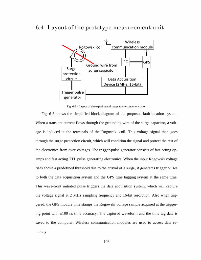
6.4 Layout of the prototype measurement unit
Fig. 6-3 - Layout of the experimental setup at one converter station
Fig. 6-3 shows the simplified block diagram of the proposed fault-location system.
When a transient current flows through the grounding wire of the surge capacitor, a volt-
age is induced at the terminals of the Rogowski coil. This voltage signal then goes
through the surge protection circuit, which will condition the signal and protect the rest of
the electronics from over voltages. The trigger-pulse generator consists of fast acting op-
amps and fast acting TTL pulse generating electronics. When the input Rogowski voltage
rises above a predefined threshold due to the arrival of a surge, it generates trigger pulses
to both the data acquisition system and the GPS time tagging system at the same time.
This wave-front initiated pulse triggers the data acquisition system, which will capture
the voltage signal at 2 MHz sampling frequency and 16-bit resolution. Also when trig-
gered, the GPS module time stamps the Rogowski voltage sample acquired at the trigger-
ing point with ±100 ns time accuracy. The captured waveform and the time tag data is
saved to the computer. Wireless communication modules are used to access data re-
motely.
Rogowski coil
Ground wire from surge capacitor
GPSPC
Wireless communication module
Data Acquisition Device (2MHz, 16-bit)
Surge protection
circuit
Trigger pulse generator
108
6.4.1 Specifications of the Rogowski coil
Model No A(min) B(max) C(max) D(max)
TSR 35 35.0 mm 83.0 mm 20.9 mm 99.5 mm
Model No Rated Current Self Inductance Mutual Inductance DC Resistance
TSR 35 1000A 0.54 mH 0.40 µH 49 Ω
Fig. 6-4 - Technical details of the selected Rogowski coil (Redrawn from [56] )
A clamped-on Rogowski coil is selected since it is easier to install with minimum in-
terference to the existing wirings. Taehwatrans part number TSR35L [56] is selected af-
ter considering the trade-off between the availability and high mutual inductance. The
specifications are shown in Fig. 6-4. This device does not contain an integrator circuit
since there is no need to measure the actual current in the primary wire in the proposed
fault-location method. Identification of the travelling-wave arrival time is the main pur-
pose of the transducer. To improve the accuracy, it is important to see a sharper change
and measurable voltage at the Rogowski coil terminals. Generally, higher mutual induc-
A
B
D
C
TSR 35L
109

tance would produce higher voltage output at the terminal and smaller self-inductance
would provide sharper rise time.
Fig. 6-5 - Test network modeled in PSCAD/EMTDC
Fig. 6-6 - Surge capacitor current after applying a fault 1 km from rectifier (a) complete view of the two end surge ca-pacitor currents (b) zoomed in view to show the inverter end surge capacitor current
Before the selection of model TSR35L, a comparison of the response of different
Rogowski coil models listed in [56] was carried out using simulations. The relevant pa-
55nF Surge capacitor
Inverter end
Smoothing reactor
DC filters Converters
1000 km of OH line
AC system
Smoothing reactor
Rectifier end
Smoothing reactor
DC filtersConverters
Smoothing reactor
AC system
Pole 1
Pole 2
0 1 2 3 4 5
x 104
-4
-3
-2
-1
0
1
2
3
(a) Samples
Surg
e Ca
p.Cu
rrent
(kA)
Rectifier endInverter end
3.5 4 4.5
x 104
-0.12
-0.1
-0.08
-0.06
-0.04
-0.02
0
0.02
(b) Samples
Surg
e Ca
p.Cu
rrent
(kA)
Rectifier endInverter end
110

rameters (mutual and self-inductances) of the different Rogowski coils are listed in Table
6-1. The Rogowski coils were modelled in MATLAB and a HVDC system with a 1000
km long overhead line was modelled in PSCAD/EMTDC. The test network used for
simulation is shown in Fig. 6-5 and it is a modified version of the Cigre benchmark test
network. Fig. 6-6 shows the monitored surge capacitor current after applying a solid line
to ground fault 1 km away from the inverter side. The transient currents through the surge
capacitor current closer to the fault are larger and the currents observed at the other end
are comparatively smaller. The smaller current waveform measured at the far end
(somewhat close to the worst case current) is applied to the Rogowski coil models and
the output voltages are shown in Fig. 6-7.
According to Fig. 6-7(b), the TFR Rogowski coil gives sharper change and the largest
peak among the compared models and it also has highest mutual inductance as listed in
Table 6-1. Therefore, it is the ideal device to use in the experimental fault locator. The
second best coil is TSR 145 as it gives the second best ‘peak’ and the second best ‘rise
time’. However these Rogowski coils were not available to order from the manufacturer
at the time of development. According to the availability, the third best Rogowski coil
(TSR 35) was selected.
111

Rog
owsk
i coi
l vol
tage
(v)
(a) (b)
Fig. 6-7 - Comparison of Rogowski coil output voltages (a) Complete view (b) Zoomed in view to clearly show the first slope
Table 6-1 - Self and mutual inductance values of different Rogowski coils
Part No Mutual Inductance Self Inductance TSR 35 0.40 µH 0.54 mH
TSR 115 0.30 µH 1.20 mH
TSR 145 0.43 µH 1.70 mH
TFR 1 0.55 µH 3.50 mH
The Rogowski coil installed on the surge capacitor grounding wire at the Dorsey convert-
er station is shown in Fig. 6-8.
4.43 4.435 4.44 4.445 4.45 4.455 4.46 4.465 4.47
x 104
-16
-14
-12
-10
-8
-6
-4
-2
0
TFRTSR35TSR115TSR145
Rog
owsk
i coi
l vol
tage
(v)
Samples Samples
4.3 4.35 4.4 4.45 4.5 4.55 4.6 4.65
x 104
-15
-10
-5
0
5
10
TFRTSR35TSR115TSR145
112
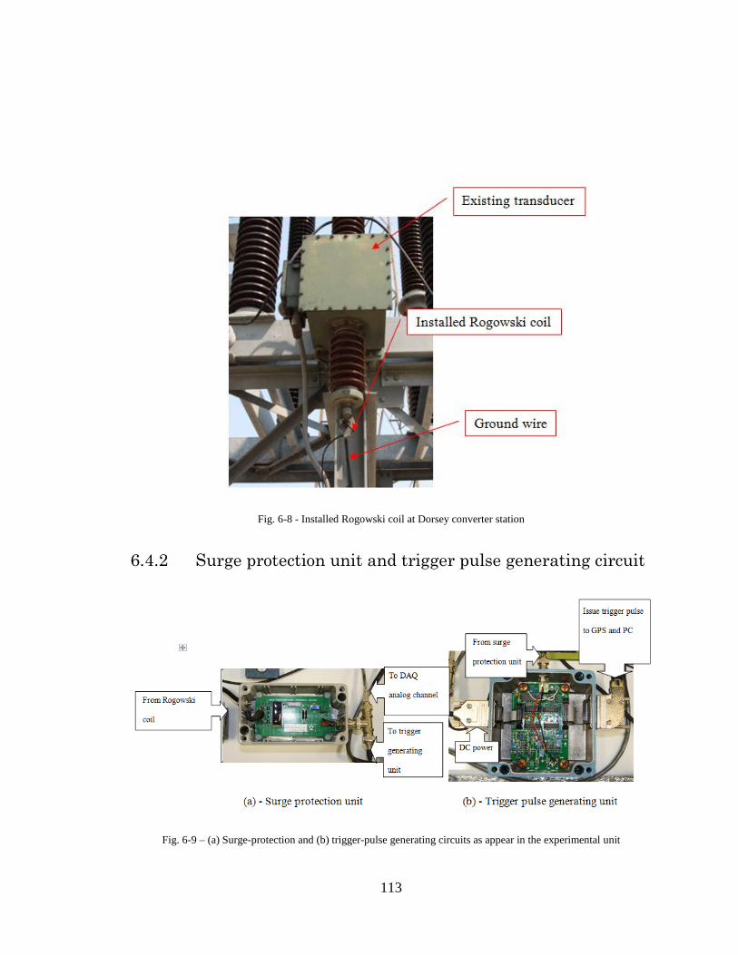
Fig. 6-8 - Installed Rogowski coil at Dorsey converter station
6.4.2 Surge protection unit and trigger pulse generating circuit
Fig. 6-9 – (a) Surge-protection and (b) trigger-pulse generating circuits as appear in the experimental unit
113

Fig. 6-9 (a) and Fig. 6-9 (b) show the surge protection unit and the trigger pulse gen-
erating unit installed in the experimental fault locator. As shown in Fig. 6-9 (a) the input
to the surge protection unit is the Rogowski coil voltage; and its output is connected to
the analog input channel of the data acquisition (DAQ) hardware and the trigger generat-
ing unit.
Main purposes of the surge protection unit are:
(1) Protect DAQ hardware and other circuits from over voltages - Protection is achieved
by two high speed Zener diodes at two voltage steps.
(2) Rectify the voltage signal arriving from the Rogowski coil - Using full diode bridge.
Rectification is required to ensure the fault locator operation for faults occurring at
both poles of Nelson River HVDC system.
As shown in Fig. 6-9 (b) the input to the trigger pulse generating unit is the output of the
surge protection unit, which is connected to both the DAQ trigger port and the trigger
port of the GPS unit.
Main purposes of the trigger generating unit are:
(1) Generate trigger pulse to the GPS unit and the DAQ hardware at the same time
when the Rogowski coil voltage is larger than a threshold. This will ensure the time
tag given from the GPS unit perfectly matches with the trigger point of the DAQ
unit.
(2) Hold the trigger pulse for 40 ms to make the system immune to the miss-triggers.
114
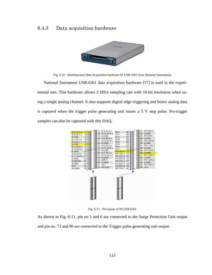
6.4.3 Data acquisition hardware
Fig. 6-10 - Multifunction Data Acquisition hardware NI USB-6361 from National Instruments
National Instrument USB-6361 data acquisition hardware [57] is used in the experi-
mental unit. This hardware allows 2 MS/s sampling rate with 16-bit resolution when us-
ing a single analog channel. It also supports digital edge triggering and hence analog data
is captured when the trigger pulse generating unit issues a 5 V step pulse. Pre-trigger
samples can also be captured with this DAQ.
Fig. 6-11 - Pin layout of NI USB 6361
As shown in Fig. 6-11, pin no 1 and 6 are connected to the Surge Protection Unit output
and pin no. 73 and 90 are connected to the Trigger pulse generating unit output.
115
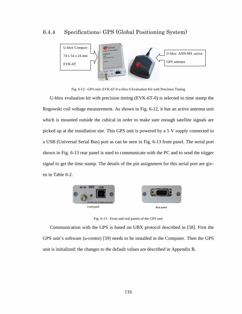
6.4.4 Specifications: GPS (Global Positioning System)
Fig. 6-12 - GPS unit: EVK-6T-0 u-blox 6 Evaluation Kit with Precision Timing
U-blox evaluation kit with precision timing (EVK-6T-0) is selected to time stamp the
Rogowski coil voltage measurement. As shown in Fig. 6-12, it has an active antenna unit
which is mounted outside the cubical in order to make sure enough satellite signals are
picked up at the installation site. This GPS unit is powered by a 5 V supply connected to
a USB (Universal Serial Bus) port as can be seen in Fig. 6-13 front panel. The serial port
shown in Fig. 6-13 rear panel is used to communicate with the PC and to send the trigger
signal to get the time stamp. The details of the pin assignment for this serial port are giv-
en in Table 6-2.
Fig. 6-13 - Front and real panels of the GPS unit
Communication with the GPS is based on UBX protocol described in [58]. First the
GPS unit’s software (u-centre) [59] needs to be installed in the Computer. Then the GPS
unit is initialized: the changes to the default values are described in Appendix B.
U-blox ANN-MS active
GPS antenna
U-blox Compact
74 x 54 x 24 mm
EVK-6T
116

Table 6-2 - Serial communication pin assignment
Pin No Assignment 1 GPS Time Pulse Output
2 GPS Transmit Data
3 GPS Receive Data
4 GPS External Trigger
5 Ground
6 GPS Time Pulse Output 2
7-9 Not Used
6.4.5 Specifications: Personal computer and the wireless
communication module
Wireless Communication module
Fig. 6-14 - IPn3G - 3G Cellular Ethernet/Serial/USB Gateway
A 3G cellular Ethernet gateway (Cellular Radio IPn3G -3G Cellular
Ethernet/Serial/USB Gateway from Microhard Corp) is used to provide internet access to
the computer deployed in the field which is shown in Fig. 6-14. The details of this device
can be found in [63] and a separate Yagi type antenna is mounted in order to capture sig-
117

nals from the weak cellular network at the station yard. Subscriber Identification Module
(SIM) with a data plan was purchased from Manitoba Telecommunication Services
(MTS). The SIM is inserted to the Cellular gateway and a PC is connected to the Cellular
gateway via an Ethernet port.
Computer
Fig. 6-15 - ARK-3360F Embedded Box PC from AdvanTech
Embedded box PC model ARK-3360F shown in Fig. 6-15 from Advantech [64] is
used as the Personal Computer in the experimental unit and Windows 7 Professional 64
bit operating system was installed. Serial port (COM 6) is used to communicate with the
GPS unit and one USB port is used to supply power to the GPS unit. The Ethernet port is
connected to the wireless gateway. Another USB port is connected to the DAQ hardware.
The GPS unit’s software u-centre version 7.02, National Instrument Measurement and
Automation Explorer version 4.7 with NI-DAQmx 9.1, and the software developed to cap-
ture the Rogowski coil waveforms are installed in the computer.
118

6.4.6 Software for capturing waveforms
Fig. 6-16 - Simplified flow diagram of the developed software
Data capturing software was written in Microsoft Visual C and C++. A simplified
flow diagram of the software is shown in Fig. 6-16. The program will read 10000 sam-
ples from the DAQ when the data is available at the DAQ buffer and the first 3000 sam-
ples are pre-trigger samples. This corresponds to a 5 ms time period at 2 MHz sampling
rate. This is more than enough to capture the first travelling-wave surges for any fault that
happened within the 895 km long OH line.
Start
Variable initialization& function declaration
Serial port initialization
Register “everyNcallback”
function
Is DAQ data received?
Read data to Aidata array
Stop analog data capturing
task
Endless loop to read serial port
Stop
Read data from serial
port
TM2 message received?
Wait for 20ms
Write RAW data to CSV
file
Wait for 200ms
No
Yes
Yes No
Exit loop to end program
Continue loop
Process 1 – Read serial port for GPS data
Process 2 – Read DAQ data
Process 1Process 2
Create analog channel with digital edge
triggering
119
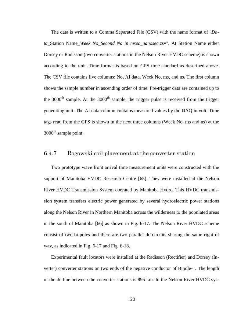
The data is written to a Comma Separated File (CSV) with the name format of "Da-
ta_Station Name_Week No_Second No in msec_nanosec.csv". At Station Name either
Dorsey or Radisson (two converter stations in the Nelson River HVDC scheme) is shown
according to the unit. Time format is based on GPS time standard as described above.
The CSV file contains five columns: No, AI data, Week No, ms, and ns. The first column
shows the sample number in ascending order of time. Pre-trigger data are contained up to
the 3000th sample. At the 3000th sample, the trigger pulse is received from the trigger
generating unit. The AI data column contains measured values by the DAQ in volt. Time
tags read from the GPS is shown in the next three columns (Week No, ms and ns) at the
3000th sample point.
6.4.7 Rogowski coil placement at the converter station
Two prototype wave front arrival time measurement units were constructed with the
support of Manitoba HVDC Research Centre [65]. They were installed at the Nelson
River HVDC Transmission System operated by Manitoba Hydro. This HVDC transmis-
sion system transfers electric power generated by several hydroelectric power stations
along the Nelson River in Northern Manitoba across the wilderness to the populated areas
in the south of Manitoba [66] as shown in Fig. 6-17. The Nelson River HVDC scheme
consist of two bi-poles and there are two parallel dc circuits sharing the same right of
way, as indicated in Fig. 6-17 and Fig. 6-18.
Experimental fault locators were installed at the Radisson (Rectifier) and Dorsey (In-
verter) converter stations on two ends of the negative conductor of Bipole-1. The length
of the dc line between the converter stations is 895 km. In the Nelson River HVDC sys-
120
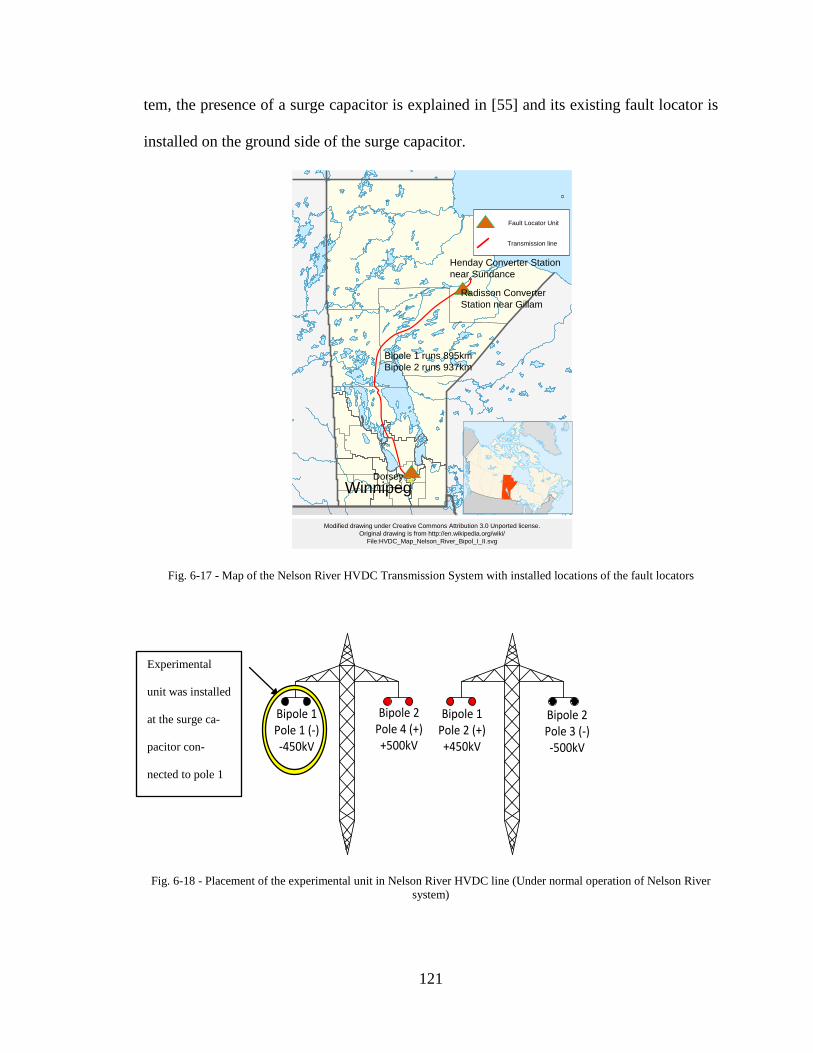
tem, the presence of a surge capacitor is explained in [55] and its existing fault locator is
installed on the ground side of the surge capacitor.
Fig. 6-17 - Map of the Nelson River HVDC Transmission System with installed locations of the fault locators
Fig. 6-18 - Placement of the experimental unit in Nelson River HVDC line (Under normal operation of Nelson River system)
Dorsey
Radisson Converter Station near Gillam
Henday Converter Station near Sundance
Bipole 1 runs 895kmBipole 2 runs 937km
Winnipeg
Modified drawing under Creative Commons Attribution 3.0 Unported license. Original drawing is from http://en.wikipedia.org/wiki/
File:HVDC_Map_Nelson_River_Bipol_I_II.svg
Fault Locator Unit
Transmission line
Bipole 1Pole 1 (-)-450kV
Bipole 2Pole 4 (+)+500kV
Bipole 1Pole 2 (+)+450kV
Bipole 2Pole 3 (-)-500kV
Experimental
unit was installed
at the surge ca-
pacitor con-
nected to pole 1
121

6.5 Summary of the recorded events
Fig. 6-19 - Venn diagram view of recorded events
The distribution of the number of events recorded in the experimental unit and the
operational fault locator between the 23rd of July and the 4th of September in 2012 are
shown in Fig. 6-19. During this time period, only temporary dc line faults were recorded.
Thus the actual location of any of the events could not be verified by physical observa-
tion. However, locations of 25 events were verified with the existing operational fault lo-
cator. A histogram of the distance to fault-location from Dorsey station of the 25 verified
events are shown in Fig. 6-20. About 52% of the events occurred between 550 km to 700
km from Dorsey station. No events were recorded within 400 km from Dorsey station.
Similarly no events were recorded beyond 825 km from Dorsey station.
Fig. 6-20 - Histogram view of the fault-location from Dorsey in Kilometers
25
Existing LFL: AExperimental LFL: B
AB
15
350 400 450 500 550 600 650 700 750 800 8500
1
2
3
4
5
6
7
8
9
Fault location from Dorsey in km
No o
f eve
nts
122

The waveforms captured during event 1 are shown in Fig. 6-21. This temporary fault
happened about 825 km from Dorsey station and the event was verified with the opera-
tional fault-location unit. It is evident from Fig. 6-21 that this event generated Rogowski
coil voltages which are easily measurable from the DAQ units at both ends, even though
the fault was close to the Radisson end of the line. Table 6-3 compares the fault locations
determined by the prototype unit and the operational unit. The mismatch in the measured
surge-arrival time difference is 646 ns. The difference in the estimated fault-location is
0.09 km for this particular event.
Fig. 6-21 - Captured waveform from the experimental unit (First recorded event)
Table 6-3 - Comparison of fault-location & surge-arrival time difference of event 1
Fault-location in km from Dorsey Wave-front arrival time differ-
ence between two units (nsec) Operational unit Experimental unit
826.25 826.16 646.0057
-6000 -4000 -2000 0 2000 4000 6000 8000 10000 12000-2
0
2
4
6
8
10
Samples
Rog
owsk
i coi
l vol
tage
(V
)
Event no: 1 (825km from Dorsey)
DorseyRadisson
123

Voltages of all the captured waveforms from the experimental unit are shown on a
colour map in Fig. 6-22. In the colour maps, the horizontal axis represents the sample
numbers and the sampling process was done at a 2 MHz sampling rate. The vertical axis
shows the event number in ascending order of time and the colour scale represents the
Rogowski coil voltage in volts.
Fig. 6-22 - Colour map view of captured Rogowski coil voltages in volts
2995 3000 3005 3010 3015 3020
5
10
15
20
25
Samples
Eve
nts
Dorsey rogowski coil voltages
0
1
2
3
4
5
6
7
2995 3000 3005 3010 3015 3020
5
10
15
20
25
Samples
Eve
nts
Radisson rogowski coil voltages
0
1
2
3
4
5
6
7
8
9
124

Fig. 6-23 - Captured Rogowski coil pre fault voltages for selected events
Noise level present in the system can be observed with pre-fault voltages and the noise
level can be varied due to many factors like the operating conditions, weather conditions
and external communication interferences etc. However, for the Nelson River System
during the observed periods, the noise levels were within ±20 mV range as can be seen in
Fig. 6-23. Noise level is smaller compared to the voltage peak which appeared at the
wave-front arrival point. According to Fig. 6-22, rise time of the signal is within 10 sam-
ples (At 2 MHz rate this value is equal to 5 μs time period) for most of the cases. There-
fore the proposed Rogowski coil transducer is suitable in the Nelson River HVDC dc line
fault-location application.
1000 1200 1400 1600 1800 2000-0.02
-0.015
-0.01
-0.005
0
0.005
0.01
0.015
sample
Vol
tage
Event no: 2
DorseyRadisson
5000 5200 5400 5600 5800 6000-0.02
-0.015
-0.01
-0.005
0
0.005
0.01
0.015
sample
Vol
tage
Event no: 2
1000 1200 1400 1600 1800 2000-0.02
-0.015
-0.01
-0.005
0
0.005
0.01
0.015
sample
Vol
tage
Event no: 23
5000 5200 5400 5600 5800 6000-0.015
-0.01
-0.005
0
0.005
0.01
sample
Vol
tage
Event no: 23
125
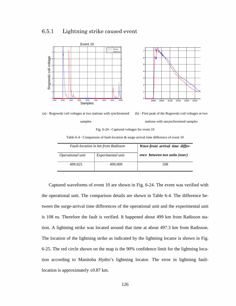
6.5.1 Lightning strike caused event
(a) - Rogowski coil voltages at two stations with synchronized
samples
(b) - First peak of the Rogowski coil voltages at two
stations with unsynchronized samples
Fig. 6-24 - Captured voltages for event 10
Table 6-4 - Comparison of fault-location & surge-arrival time difference of event 10
Fault-location in km from Radisson Wave-front arrival time differ-
ence between two units (nsec) Operational unit Experimental unit
499.025 499.009 108
Captured waveforms of event 10 are shown in Fig. 6-24. The event was verified with
the operational unit. The comparison details are shown in Table 6-4. The difference be-
tween the surge-arrival time differences of the operational unit and the experimental unit
is 108 ns. Therefore the fault is verified. It happened about 499 km from Radisson sta-
tion. A lightning strike was located around that time at about 497.3 km from Radisson.
The location of the lightning strike as indicated by the lightning locator is shown in Fig.
6-25. The red circle shown on the map is the 90% confidence limit for the lightning loca-
tion according to Manitoba Hydro’s lightning locator. The error in lightning fault-
location is approximately ±0.87 km.
2000 3000 4000 5000 6000 7000 8000 9000 100000
1
2
3
4
5
6
7
Event 10R
ogow
ski c
oil v
olta
ge
Samples
DorseyRadisson
3000 3050 3100 3150 3200 32500
1
2
3
4
5
6
7
126

Fig. 6-25 - Fault-location on the map obtained with Manitoba Hydro's lightning strike locator
Therefore this event is an example case of a lightning strike caused disturbance. As can
be seen in Fig. 6-24 (b), the captured waveform contains a sharp edge rising to about 7 V,
making it easier to identify the surge-arrival time with less error.
6.5.2 Identification of a disturbance occurred in pole 3
Fig. 6-26 - Nelson River HVDC system dc tower operation under normal condition
490.69km
495.35km
502.28km
Possible location of the lighting stike
1.95km
Bipole 1Pole 1 (-)-450kV
Bipole 2Pole 4 (+)+500kV
Bipole 1Pole 2 (+)+450kV
Bipole 2Pole 3 (-)-500kV
Disturbance
happened on line
connected to
pole 3
Experimental unit was
installed at the surge
capacitor connected to
pole 1
127

Fig. 6-27 - Event 3 occurred on pole 3
During the normal operation pole 3 is located towards the right side edge of the right
of way and pole 1 is located at the left side edge of the right of the way as shown in Fig.
6-26. The experimental unit is installed on pole 1. Due to mutual coupling even a fault
occurring in pole 3 can induce transient voltages on pole 1 and these transients create a
voltage at the Rogowski coil terminal which can be observed in the experimental unit. An
example event is shown in Fig. 6-27. As can be seen the peak voltages are relatively low-
er compared to the disturbances that occurred on pole 1. However this event is still clear-
ly recognizable. It was verified as a pole 3 disturbance with Sequence Event Recorder
(SER) data and also with the operational unit data.
6.6 Simulation study
The simulation study presented in this section is carried out with two objectives. The
first is to compare the wave-front arrival times directly obtained from the Rogowski coil
measurements with those obtained using the wavelet coefficients of the surge capacitor
current. The practical measurements showed that surge-arrival time can be measured with
good accuracy even from the direct comparison of the Rogowski coil output with a
1000 2000 3000 4000 5000 6000 7000 8000
0
0.5
1
1.5
2
2.5
3
3.5
4
4.5
Event 3
Rogo
wski
coi
l vol
tage
Samples
DorseyRadisson
128

threshold. If the accuracy of the wave-front arrival times directly obtained using the
Rogowski coil is comparable with those obtained through wavelet coefficients, the use of
direct measurements is preferable.
The second objective of the simulation study is to validate the application of
Rogowski coils based measurement scheme for extra-long dc transmission lines. Thus the
test HVDC network used for simulations contains a 2400 km long OH line, which is
much longer than the 895 km line of the Nelson River System. However, the simulation
model of the measurement scheme in the fault locator is similar to the experimental setup
installed at the Nelson River HVDC system.
6.6.1 Test network
A conventional two-terminal HVDC system with a 2400 km long overhead transmis-
sion line was used in simulation studies. The schematic diagram of the test network is
shown in Fig. 6-28. All the simulations were carried out with PSCAD/EMTDC and the
wavelet transform calculations and Rogowski coil modeling were performed in MAT-
LAB. The surge capacitors used in the simulation model are of 0.055 µF capacity, which
is smaller than the 0.55 µF used in the Nelson River HVDC scheme. This combination of
small surge capacitors and the extra-long transmission line represents an extremely diffi-
cult case in terms of the detection of surges. The surge capacitor currents were monitored
for dc line short circuit faults applied at different locations. Simulations were performed
in PSCAD/EMTDC with a solution time step of 0.1 µs to ensure all high frequency com-
ponents are present in the signals. This arrangement of the fault locator is similar to the
experimental setup installed at the Nelson River system.
129

Fig. 6-28 - Simulation model
6.6.2 Rogowski coil simulation model
The Electro Magnetic Transient (EMT) type Rogowski coil model proposed in [28] is
used in this study. The equivalent circuit of the simulation model is shown in Fig. 6-29.
The induced voltage is proportional to the rate of change of primary conductor current
times the mutual inductance of the Rogowski coil. The load impedance is the impedance
of the DAQ seen by the Rogowski coil, which is mostly resistive and large. In [28], this
model based on the electromagnetic transient program (EMTP) [29] concepts has been
verified through laboratory experiments. The parameters of the Rogowski coil used in the
experimental unit were used in simulation study.
Fig. 6-29 - Equivalent circuit of the Rogowski coil
2400 km of Over head line
Surge capacitor
Smoothing reactor
DC filter
Rectifier end
Converter
Current measurement
Smoothing reactor
DC filter
Inverter end
Converter
Voltage induce due to primary winding current
ML
Self InductanceSL
Coil ResistanceSR
CapacitanceCl
Load impedanceZl
(Output voltage is measured across this)
130

6.6.3 Simulation results
The surge capacitor currents when a permanent dc line fault occurred at 1 km away
from the rectifier terminal are shown in Fig. 6-30. This can be considered as a worst case
scenario since the fault occurred close to one terminal and the travelling-wave arriving at
the far end (in this case the inverter terminal) is subjected to an immense amount of at-
tenuation. Thus the magnitude of the inverter side surge capacitor currents is significantly
smaller than that at the rectifier end, and the surge capacitor current itself cannot be used
to obtain the surge-arrival time with sufficient accuracy. Therefore application of a signal
conditioning method such as CWT or use of a suitable transducer such as a Rogowski
coil is required to enhance the visibility of the surge-arrival time.
Approximately 20 mV noise was observed in the Rogowski coil measurements during
the field experiment in the Nelson River system. If a similar noise level is assumed, a
signal with a magnitude significantly higher than 20 mV is needed to recognize the arri-
val of a wave-front. Plot (g) in Fig. 6-31 shows the variation of inverter side Rogowski
coil voltage calculated with the model described in Section 6.6.2 using the inverter surge
capacitor current shown in Fig. 6-30 as the input. It is clear that the peak voltage is well
above 3 V. Therefore, even a dc line fault occurred that 2399 km away from the terminal
is recognizable using the proposed Rogowski coil based measurement scheme.
131

Fig. 6-30 - Surge capacitor currents after dc line fault occurred 1 km from the rectifier end. In the second graph y-axis is expanded to show the details of inverter side waveform
In Fig. 6-31, (a) to (f) plots show the variations of the continuous wavelet trans-
form coefficient magnitude values calculated using the inverter side surge capacitor cur-
rent shown in Fig. 6-30. Each coefficient (scale 2, 4, and 8) represents a different fre-
quency band with scale 2 corresponding to the highest frequency. In Fig. 6-31, plots (g)-
(h) show the variations of the magnitude of the Rogowski coil output voltages (obtained
using the Rogowski coil model) for the same surge capacitor current signals. CWT coef-
ficient values are measured in amperes and the Rogowski coil outputs are measured in
voltage. However, once captured through a DAQ, the initial sharp change in these signals
is used to identify the travelling-wave arrival time. Therefore, the shape of these wave-
forms is the most important feature with respect to travelling-wave based fault-location.
2.4 2.402 2.404 2.406 2.408-5
-4
-3
-2
-1
0
1
2
3
4
Samples
Sur
ge c
ap. c
urre
nt (k
A)
Surge capacitor current
InverterRectifier
2.4 2.401 2.402 2.403 2.404 2.405 2.406 2.407 2.408
-0.3
-0.25
-0.2
-0.15
-0.1
-0.05
0
0.05
Samples
Sur
ge c
ap. c
urre
nt (k
A)
Surge capacitor current
132

Fig. 6-31 - CWT coefficient magnitudes and Rogowski coil voltage magnitude obtained from surge capacitor currents at the terminals for ground fault occurred on the dc line 1 km from the rectifier station.
According to the observation data, it is clear that the shape of the magnitude of the
Rogowski coil voltage is very similar to the wavelet coefficient magnitude variation.
2.5 2.55 2.6 2.65 2.7
x 104
0
1
2
3
4(a) Inv. |Haar CWT Scale 2|
|CW
T S
cale
2| i
n A
9500 9600 9700 9800 9900 100000
500
1000
1500
2000
2500(b) Rec. |Haar CWT Scale 2|
|CW
T S
cale
2| i
n A
2.5 2.55 2.6 2.65 2.7
x 104
0
2
4
6
8
10(c) Inv. |Haar CWT Scale 4|
|CW
T S
cale
4| i
n A
9500 9600 9700 9800 9900 100000
1000
2000
3000(d) Rec. |Haar CWT Scale 4|
|CW
T S
cale
4| i
n A
2.5 2.55 2.6 2.65 2.7
x 104
0
10
20
30(e) Inv. |Haar CWT Scale 8|
|CW
T S
cale
8| i
n A
9500 9600 9700 9800 9900 100000
1000
2000
3000
4000
5000(f) Rec. |Haar CWT Scale 8|
|CW
T S
cale
8| i
n A
2.5 2.55 2.6 2.65 2.7
x 104
0
1
2
3
4(g) Inv. |Rog. Coil|
|Rog
. Coi
l. V
olt|
9500 9600 9700 9800 9900 100000
500
1000
1500
2000(h) Rec. |Rog. Coil|
|Rog
. Coi
l. V
olt|
133

6.6.4 Rogowski coil and ‘Haar’ wavelet transform
Rogowski coil output voltage is approximately proportional to the rate of change of
surge capacitor current. When finding the Haar wavelet transform coefficients, it takes
the sums and differences of every pair of numbers in the input vector and divides them by
square root of 2 as described in Appendix-A. Then, the process is repeated on the resul-
tant vector of the summed terms. Therefore coefficient value is proportional to the rate of
change in the input signal for the considered scale. Thus Rogowski coil output voltage
and the Haar wavelet transform coefficient magnitudes both indicate a change in the
surge capacitor current.
This can be explained further using the Rogowski coil transfer function. The transfer
function of the Rogowski coil can be derived using equivalent circuit shown in Fig. 6-29
as:
𝑀𝐿.𝑍𝑙. (2𝜋.𝑓. 𝒋)𝑆𝐿.𝐶𝑙.𝑍𝑙 . (2𝜋.𝑓. 𝒋)2 + (𝑆𝐿 + 𝑆𝑅.𝐶𝑙.𝑍𝑙. (2𝜋.𝑓. 𝒋) + (𝑆𝑅 + 𝑍𝑙)
Eq. 6-2
Where, ML is the Mutual inductance, Zl is the load impedance, SL is the self-inductance,
SR is the coil resistance and Cl is the capacitance. The frequency response of the transfer
function given in Eq. 6-2 is shown in Fig. 6-32, and as can be seen the combined charac-
teristic of the sensor and the sampling system is approximately equivalent to a band-pass
filter with 300 kHz to 1 MHz band frequency. The wavelet transform can also be consid-
ered as a band-pass filtering process, with each scale corresponding to a different pass
band. For example, scale 2 responses shown in Fig. 6-31 (a) and (b) contains frequencies
from 500 kHz to 1 MHz, since the sampling rate was 2 MHz. Therefore both the
134

Rogowski coil output and the scale-2 continuous wavelet transform coefficients contain
similar frequency components in the surge capacitor currents.
Fig. 6-32 - Frequency response of the Rogowski coil
6.6.5 Fault-location results
Table 6-5 compares the fault locations calculated using the direct Rogowski coil volt-
ages measurements and the scale-2 CWT coefficients of the surge capacitor currents, for
different line-to-ground faults on the dc line in the test network.
It is clearly seen from the results that both methods give a similar accuracy of fault-
location (difference within ±50 m for the cases simulated). Thus it can be concluded that
both methods provide similar results in the detection of wave-front arrival times. There-
fore, if the proposed surge-arrival time measurement scheme is used, there is no need for
further processing of the input signals using the continuous wavelet transform. Further-
0 1 106× 2 106× 3 106× 4 106× 5 106×30−
20−
10−
0
10
Rog.Coil. Freq. Response-3dB
Frequency (Hz)
Mag
nitu
de (d
B)
135

more, the simulation shows that surge-arrival times can be detected even for an overhead
transmission line as long as 2400 km, although the signals are very small.
Table 6-5 - Comparison of fault locations
Actual fault-location from Rectifier (km)
Predicted fault-location errors (meters) using different methods
Rog. Coil CWT Scale 2 1.00 157.90 157.90 10.00 197.03 197.03 100.00 140.07 140.07 157.00 64.15 64.15 251.00 -33.52 -33.52 333.00 -9.06 -9.06 850.00 14.01 14.01 1111.00 -46.60 -46.60 1200.00 0.00 0.00 1323.00 -38.01 -38.01 1400.00 -18.68 -18.68 2040.00 -108.32 -108.32 2100.00 -121.39 -121.39 2240.00 -127.00 -127.00
6.7 Concluding remarks
This chapter demonstrated the successful application of a Rogowski coil as a trans-
ducer to identify the fault initiated travelling waves on bi-pole 1 of the Nelson River
HVDC transmission line. Two experimental units were installed at the Dorsey and Radis-
son converter stations. It also validated DAQ specifications for this application.
136

Design details of the experimental DAQ system and recorded events are discussed in
detail. The implemented system provided accurate fault locations for all the events re-
cording during the period at accuracy of ± 500 m when compared with the existing fault
locator. It was verified that the experimental system could detect faults that occurred on
the other DC line in the same right of way. The noise in the system was lower (± 20 mV)
compared to the wave-front observed in the recorded events (>3 V). The wave-fronts are
clearly visible as a sharp change in voltage. The Rogowski coil voltage itself can be used
to identify the wave-front arrival time using a pre-defined threshold.
A simulation model is used to validate the application of the Rogowski coil in an ex-
tra-long (2400 km) overhead transmission system. It is found that the Rogowski coil can
be used to calculate the fault in an extra-long HVDC system within ±200 m accuracy.
Accuracy of the results is similar to the CWT based method results. The reason for this is
simulated Rogowski coil wave form magnitudes have the same waveform signatures as
the CWT coefficient magnitudes. This is expected because the Rogowski coil has a simi-
lar frequency bandwidth as one of the wavelet transform coefficients.
137

Chapter 7
Conclusions and contributions This chapter presents the conclusions of the research, summarizes the main contribu-
tions and proposes directions for future research in the area of HVDC line fault-location.
7.1 Conclusions
In this thesis, travelling-wave based dc line fault-location, specifically the synchro-
nized two ended method, was investigated in detail with the objective of extending the
range of applications to emerging situations such as very long transmission lines and ca-
bles, multi-segment transmission lines, and multi-terminal HVDC systems.
Recognizing the fact that the accuracy of the surge-arrival time difference measure-
ment is the most critical aspect that influences the accuracy of fault-location, the possibil-
ity of using wavelet transform coefficients of the potential input signals to identify the ar-
rival of travelling waves was examined through simulation studies. While the use of
DWT coefficients as suggested by some previous literature can be helpful in the detection
of wave fronts, the use of CWT coefficients, as proposed in this thesis, clearly results in
more accurate, robust, and reliable fault-location performance compared to the DWT
based methods. This is due to the fact that CWT retains the maximum time resolution re-
138
gardless of the scale of coefficients, which is very important in determining the wave
front arrival times.
Fault-location in extra-long dc transmission lines and cables was examined through
simulations. These studies indicated that faults can be successfully located in a conven-
tional LCC type HVDC system with a 2400 km OH line or a 300 km of UG cable, only
using the terminal measurements. It was also found that both line terminal voltages and
the surge capacitor currents can perform equally well as the inputs to the fault-location
algorithm. The analysis considered the effects of signal conditioning, particularly the
scaling of inputs to a 0-20 V range and the A/D conversion of input signals at a 2 MHz
sampling rate and a 16-bit resolution.
The overall accuracy of fault-location can be improved if the appropriate propagation
velocity is determined for the particular CWT scale being used, by using the data from a
test fault performed at a known location. Investigation of the impact of noise showed that
the accuracy of the proposed method can be reduced with the amount of noise present in
the measurements. However, the impact of noise can be reduced by using CWT coeffi-
cients of higher scales (Scales 16 and 32 at 2 MHz sampling rate) without undue effect on
the fault-location accuracy.
In this research, a novel algorithm was developed to locate the faults in HVDC
transmission lines with multiple segments, using only the terminal measurements. A
theoretical derivation of the algorithm was presented and its application was validated us-
ing a three segment (OH line/UG Cable/OH line) dc transmission system simulated in
PSCAD/EMTDC. Using the proposed algorithm, it is possible to correctly identify the
faulted segment as well as the exact fault-location using only the terminal measurements.
139

Therefore the need for installation of fault-location equipment at the segment boundaries
is eliminated. Although the algorithm development and validation considered a three
segment dc transmission system, the proposed fault-location algorithm can be generalized
to a dc transmission system with any number of segments as long as the measurement of
the surge-arrival time difference is practical.
Furthermore, a new fault-location algorithm was developed for VSC based star con-
nected multi-terminal HVDC schemes. The proposed algorithm is also based on the trav-
elling-wave fault-location principle and it has the ability to correctly identify the faulted
line segment and fault-location using only the measurements at the converter station
ends. This was validated for a 3-terminal VSC HVDC system consisting of overhead line
segments through simulation studies. The proposed method eliminates the need for the
installation of repeater stations at the junction of the multi-terminal HVDC network. Al-
though derivations and simulations were carried out considering a three-terminal dc net-
work, the concept can be expanded to general network with any number of terminals as
long as surge-arrival time measurements are available at the converter stations.
Finally, an experimental measurement system was developed for identifying the arri-
val of fault initiated travelling waves. This measurement system that uses a Rogowski
coil as a transducer was field tested on the dc line connecting Dorsey and Radisson con-
verter stations of the Nelson River HVDC transmission system in Manitoba, Canada. The
field measurements showed that the proposed measurement scheme can accurately detect
the surge-arrival times, even without the post processing of the signals, in this nearly
1000 km long overhead transmission system. The noise in the practical measurements
was very low (± 20 mV) compared to the magnitudes of the wave-fronts observed in the
140

recorded events (>3 V), and the wave-fronts were clearly distinguishable. Furthermore, it
was verified that the experimental system could detect the faults that occurred on a paral-
lel dc line in the same right of way, using the induced transients. A simulation model
was used to investigate the applicability of the Rogowski coil based measurement system
for fault-location on an extra-long overhead transmission system. It was found through
the simulation studies that the proposed measurement scheme, which directly uses the
output of the Rogowski coil transducer to detect surge-arrival times, can determine the
fault locations in a 2400 km long HVDC system line with a ± 200 m accuracy. This accu-
racy is similar to the results obtained using the CWT coefficients of the surge capacitor
currents. Further analysis showed that the Rogowski coil output waveforms have a wave-
form signature similar to that of the CWT coefficients.
It is hoped that the outcomes of the thesis would be beneficial to the power industry,
as the developed algorithms could be incorporated to enhance the capabilities of the ex-
isting dc line fault locators. The knowledge gained through the project was dispersed
through scientific publications.
7.2 Contributions
Main contributions of the research are:
1. Development of an improved method to detect the travelling-wave arrival times
using the continuous wavelet transform coefficients. This can improve the accu-
racy and reliability of travelling-wave based fault-location compared to discrete
wavelet transform based method.
2. Assertion that the dc line terminal voltages and the surge capacitor currents are
the most suitable input signals for detecting the travelling waves in both overhead
line and cable based HVDC transmission systems that use line commutated con-
141

verters. The same signals will work for voltage source converter based HVDC
systems if a small series reactance is present at the dc line terminals; otherwise the
dc line current can be used as an input signal although measurement is practically
difficult.
3. Development of a new algorithm for fault-location in classical two-terminal
HVDC schemes with multiple segments of OH lines and UG cables using only
the measurements at two ends. The algorithm is simple to implement and inde-
pendent of the method of measurement of travelling-wave arrival times. This find-
ing has significant potential to reduce the cost of fault-location in HVDC trans-
mission systems with multiple segments in comparison to the current technology
that uses repeater stations at segment boundaries.
4. Development of a new algorithm for fault-location in star connected multi-
terminal HVDC schemes using only measurements at the converter terminals.
This algorithm is also simple to implement and independent of the travelling-
wave arrival time measurement method. This finding will enable efficient fault-
location in multi-terminal HVDC grids that are being considered for various ap-
plications such as the harnessing of offshore wind resources.
5. Development of a robust measurement scheme for the detection of travelling-
wave arrival times using Rogowski coils, and validation of its practicality through
field tests in a real HVDC transmission system. .
These contributions led to the following publications in journals and conferences.
• O. M. K. K. Nanayakkara, A. D. Rajapakse, and R. Wachal, “Fault Location in HVDC
Transmission Lines Using Discrete Wavelet Transform,” presented at the Cigre Canada
Conference on Power Systems 2010, Vancouver, Canada, 2010.
• K. Nanayakkara, A. D. Rajapakse, and R. Wachal, “Fault location in extra long HVDC
transmission lines using continuous wavelet transform,” presented at the International
Conference on Power Systems Transients (IPST), Delft, the Netherlands, 2011.
142

• O. M. K. K. Nanayakkara, A. D. Rajapakse, and R. Wachal, “Location of dc Line Faults
in Conventional HVDC Systems With Segments of Cables and Overhead Lines Using
Terminal Measurements,” IEEE Transactions on Power Delivery, vol. 27, no. 1, pp. 279–
288, Jan. 2012.
• O. M. K. K. Nanayakkara, A. D. Rajapakse, and R. Wachal, “Travelling-Wave-Based
Line Fault Location in Star-Connected Multiterminal HVDC Systems,” IEEE Transac-
tions on Power Delivery, vol. 27, no. 4, pp. 2286 –2294, Oct. 2012.
7.3 Suggestions for future research
This research is based on fault-location in dc lines that are used to deliver electrical
power. In some HVDC systems, the grounding electrode is located at a remote destina-
tion and the operators may require the location of faults and discontinuities in the line
connecting to the ground electrode. Since there is no current flowing in the electrode
lines under normal operation, the methods proposed in this thesis are not applicable. Fur-
ther investigations are necessary to develop suitable methods for electrode line fault-
location.
With the advancement of telecommunication technology, the physical size of GPS
units and DAQ systems are becoming more miniature and their accuracies are improving.
Field-programmable gate array (FPGA) technology is developing at a rapid rate and there
is a potential to develop compact dc line fault locators by combing a FPGA unit, a GPS
unit, a wireless communication unit, and a Rogowski coil transducer into a single module
which can be easily deployed in the converter station yard.
It was revealed that the Rogowski coil can be used to detect travelling waves at high
accuracy in HVDC systems. Therefore Rogowski coils can be used in travelling-wave
143

based relays as the main transducer instead of a standard current transformer. The pro-
posed multi-terminal fault-location algorithm can be adapted to locate faults in the teed
ac transmission networks.
144

Appendix A: Wavelet Transform
A.1 Introduction
Main challenge in travelling-wave based fault-location is the determination of the
precise times of arrival of travelling waves by analyzing the high frequency content of a
measured input signal. Short-Time Fourier transform (STFT) is a modified version of
classical Fourier transform which uses a window function to provide time-frequency
analysis. Although STFT can be used to observe singularity point in a monitored signal,
there are still limitations when it comes to fault location applications due to the fixed res-
olution arising from the fixed width of the window function.
Wavelet transform is similar to STFT and it provides time-frequency analysis by
changing the location and scaling of a mother wavelet, which is the window function in
Wavelet transform. Wavelet transform can capture short-duration, high frequency and
long-duration, low frequency information simultaneously and therefore useful for singu-
larity detection with noisy signals as explained in Section 3.5.
The continuous wavelet transform (CWT) is a correlation between the analyzed sig-
nal and a wavelet at different scales and hence provides similarity between the input-
145

signal with the mother wavelet at the scale being used. The CWT was computed by se-
lecting the scale of the analysis window, multiplying it by the input signal, and integrat-
ing the product over the time. This is repeated after shifting the window in time by one
sample time at each step, Discrete Wavelet Transform (DWT) coefficients are usually
sampled from the CWT on a dyadic grid so the scaling and shifting is based on power of
two. In this appendix, shape of Haar wavelet and calculation steps of the Haar wavelet
transform are explained.
A.2 Haar wavelet
The Haar transform is the simplest of the wavelet transforms and it finds inner prod-
uct between the input signal and the shifted and scaled versions of the Haar mother wave-
let. Haar wavelet coefficients basically calculate the difference (gradient) in the input
signal at each scale level. Fig. A-1 shows the Haar mother wavelet shape and its shifting
process and Fig. A-2 shows a comparison of Haar wavelet shapes at scales 2, 4 and 8.
Mathematical function of the Haar wavelet is shown in Eq. A-1.
Eq. A-1
146

Fig. A-1 - Haar wavelet and its shifting process
As the scale goes up, the width of the Haar wavelet increases and hence the Haar wavelet
transform gives lower frequency variations in the input signal. Fig. A-3 compares an ex-
ample waveform of the surge capacitor current after a fault with the original Haar mother
wavelet and scale 32 version of the Haar wavelet. The original Haar mother wavelet is
more sensitive to sudden variations of the signal and gives more time resolution. Howev-
er, it is more likely to respond to high frequency noise in the case of practical signal. On
the other hand scale 32 is could be robust against high frequency noise. As the scale is in-
creasing, the wavelet will become less sensitive to sudden changes. Thus a suitable scale-
should be selected as a compromise between these two aspects.
1 2 3 4 5
1−
0
1
x
haar
(x-1
)
1 2 3 4 5
1−
0
1
x
haar
(x-2
)1 2 3 4 5
1−
0
1
x
haar
(x-3
)
1 2 3 4 5
1−
0
1
x
haar
(x-4
)
147

Fig. A-2 - Haar wavelets at different scales
Fig. A-3 – Comparison of Haar wavelet and its scale 32 version with an example surge capacitor current signal
2 4 6 8 10
1−
0
1
x
Haa
r wav
elet
2 4 6 8 10
1−
0
1
x
Scale
2 Ha
ar wa
velet
2 4 6 8 10
1−
0
1
x
Scal
e 4
Haa
r wav
elet
2 4 6 8 10
1−
0
1
x
Scal
e 8
Haa
r wav
elet
0 10 20 30 402−
1−
0
1
Surge capacitor current (kA)Haar mother waveletScale 32 Haar wavelet
Time
Mag
nitu
de
148

A.3 Example calculation of Haar wavelet
coefficients
Steps to calculate Haar wavelet transform of an array of n samples is as follows:
Consider the array as n/2 pairs with samples i and i+1 together where i is an even
sample number.
• Calculate addition of each pair (ith + (i+1)th) and divide that value by √2. These
values will be the approximate coefficients.
• Calculate difference between ith and (i+1)th samples for each pair and divide that
value by √2. These values will be the detail coefficients.
• Consider the approximate coefficients as inputs and repeat the process to get next
level of detail coefficients.
Example calculation:
The input signal is given in the first column of Table A-1 and in Fig. A-4. Following the
above mentioned steps, the Haar wavelet approximate and detail coefficients (Fig. A-5 )
are calculated for the input signal.
Table A-1 – Example of calculated Haar wavelet coefficients
Level 1 Level 2 Level 3
Input signal Approximate coefficient
Detail coeffi-cient
Approximate coefficient
Detail coeffi-cient Detail coefficient
1 2 2.121320344 -0.70710678 3 1 2.828427125 1.414213562 3.5 -0.5 2 3 3.535533906 -0.70710678 4 0 2.828427125 2.828427125 4.5 0.5 -0.70710678
149
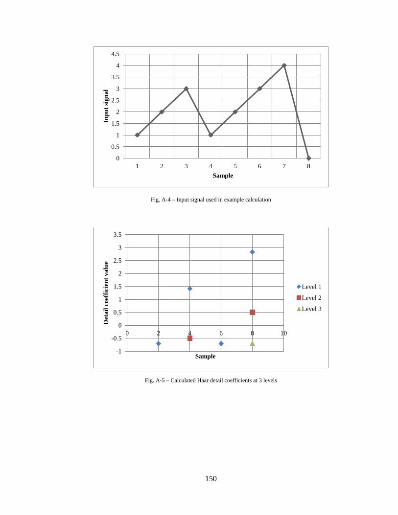
Fig. A-4 – Input signal used in example calculation
Fig. A-5 – Calculated Haar detail coefficients at 3 levels
0
0.5
1
1.5
2
2.5
3
3.5
4
4.5
1 2 3 4 5 6 7 8
Inpu
t sig
nal
Sample
-1
-0.5
0
0.5
1
1.5
2
2.5
3
3.5
0 2 4 6 8 10
Det
ail c
oeff
icie
nt v
alue
Sample
Level 1
Level 2
Level 3
150
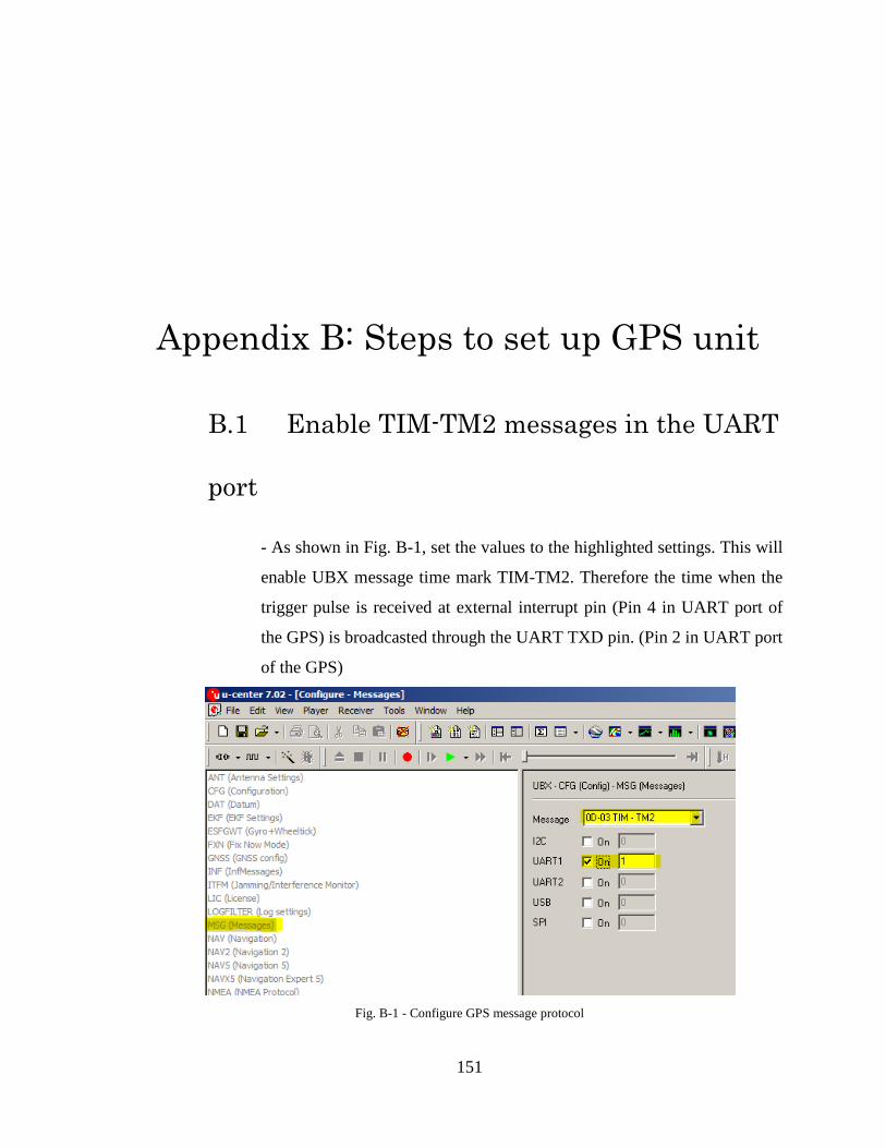
Appendix B: Steps to set up GPS unit
B.1 Enable TIM-TM2 messages in the UART
port
- As shown in Fig. B-1, set the values to the highlighted settings. This will
enable UBX message time mark TIM-TM2. Therefore the time when the
trigger pulse is received at external interrupt pin (Pin 4 in UART port of
the GPS) is broadcasted through the UART TXD pin. (Pin 2 in UART port
of the GPS)
Fig. B-1 - Configure GPS message protocol
151
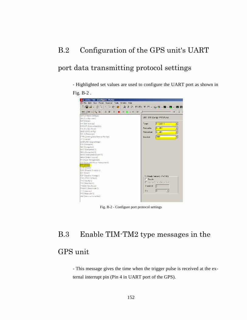
B.2 Configuration of the GPS unit's UART
port data transmitting protocol settings
- Highlighted set values are used to configure the UART port as shown in
Fig. B-2 .
Fig. B-2 - Configure port protocol settings
B.3 Enable TIM-TM2 type messages in the
GPS unit
- This message gives the time when the trigger pulse is received at the ex-
ternal interrupt pin (Pin 4 in UART port of the GPS).
152

Fig. B-3 - Enable TIM-TM2 messages
B.4 Location calibration of the GPS unit
- At the installation site after mounting the GPS antenna and the unit in
the field, the GPS unit needs to be calibrated for the location.
-As shown in Fig. B-3, the location of the GPS unit can be calibrated
by running survey-in. Once the location is fixed the unit automatically
changes the time mode to "2 - Fixed mode" and shows the fixed time
mode true position (ECEF). Time taken for this process is dependent on
the satellite signal strength.
153

Fig. B-4- GPS survey-in
GPS time format is used in both the GPS unit and the developed software. The GPS time
count began at 00:00:00 of 06 January 1980 in Coordinated Universal Time (UTC) [61].
It usually represented in week no portion and seconds portion. The U-blox GPS time
mark message (TIM TM2) gives trigger time in three parts: Week No, milliseconds and
nanoseconds. At the moment GPS time is ahead by 16 seconds to the UTC time [62].
154

References [1] S. Patel. (2007, April), “The Age of the 800-kV HVDC,” IEEE power & energy
magazine [Online] Available: http://www.powermag.com/issues/departments/global_monitor/The-Age-of-the-800-kV-HVDC_2450.html
[2] B. Backwell. (2009, July), “ABB wins contract for world's longest HVDC link,” Recharge [Online] Available: http://www.rechargenews.com/energy/wave_tidal_hydro/article184870.ece
[3] T. Westerweller and J. Price, “Crossing the divide [Basslink HVDC interconnector],” Power Engineer, vol. 20, pp. 42-45 , Oct. 2006
[4] “ABB NorNed - ABB HVDC Reference Projects in Europe (HVDC References),” ABB [Online].Available: http://www.abb.com/industries/ap/db0003db004333/4ada587c75f8d975c125774a00422545.aspx.
[5] L. Tang and B. T. Ooi, “Locating and Isolating dc Faults in Multi-Terminal dc Systems”, IEEE Transactions on Power Delivery, vol. 22,no. 3, pp. 1877-1884, July 2007.
[6] “ABB HVDC Light - HVDC (Power T&D Solutions),” ABB [Online]. Available: http://www.abb.ca/industries/us/9AAC30300394.aspx.
[7] “HVDC MaxSine® | ALSTOM GRID,” Alstom [Online]. Available: http://www.alstom.com/grid/products-and-services/engineered-energy-solutions/hvdc-transmission-systems/HVDC-MaxSine/
[8] “HVDC PLUS (VSC Technology) - Siemens,” Siemens [Online]. Available: http://www.energy.siemens.com/hq/en/power-transmission/hvdc/hvdc-plus
[9] M. G. Bennett, N.S. Dhaliwal and A.Leirbukt, “A survey of the reliability of hvdc systems throughout the world during 2009-2010,” presented at the Cigre B4 2012, Paris, France, 2012.
[10] M. D. Heffernan, J. Arrillaga, K.S. Turner and C.P. Arnold “Recovery from Temporary H.V.D.C. Line Faults,” IEEE Transactions on Power Apparatus and Systems, vol. PAS-100, no. 4, pp. 1864–1870, April 1981.
[11] C. W. Taylor and S. Lefebvre, “HVDC controls for system dynamic performance,” IEEE Transactions on Power Systems, vol. 6, no. 2, pp. 743–752, May 1991.
155

[12] PSE POLNOC HVDC SwePol Link, “www.pse-swepollink.pl.” [Online].
Available: http://www.pse-swepollink.pl/awariee.html.
[13] M.M. Saha, J.J. Izykowski and E. Rosolowski, Fault location on power networks, Springer, 2010.
[14] J. Suonan, Shuping Gao, Guobing Song, Zaibin Jiao and Xiaoning Kang, “A Novel Fault-Location Method for HVDC Transmission Lines,” IEEE Transactions on Power Delivery, vol. 25, no. 2, pp. 1203–1209, April 2010.
[15] M. Shukr, D.W.P. Thomas and P. Zachetta, “VSC-HVDC transmission line faults location using active line impedance estimation,” IEEE International Conference on Energy (ENERGY CON), pp. 244–248, Sept. 2012.
[16] M. Ramesh and A. J. Laxmi, “Fault identification in HVDC using artificial intelligence - Recent trends and perspective,” International Conference on Power, Signals, Controls and Computation (EPSCICON), pp. 1–6, Jan. 2012.
[17] T. Westerweller and J.J. Price, “Basslink HVDC interconnector-system design considerations,” The 8th IEE International Conference on ac and dc Power Transmission (ACDC 2006), pp. 121–124, 2006.
[18] S. Sasaki, “Suppression of Abnormal Overvoltages on a Metallic Return HVDC Overhead Line/Cable Transmission System,” IEEE Transactions on Power Apparatus and Systems, vol. PAS-94, no. 5, pp. 1925–1934, Sept/Oct 1978.
[19] L. Tang and B. Ooi, “Protection of VSC-Multi-Terminal HVDC against dc Faults”, Power Electronics Specialists Conference 2002, Vol. 2, pp. 719-724, 2002.
[20] T.W. Radford, “HVDC line fault locator upgrade”, in Proc. HVDC operating conference, pp. 189-200, 1987.
[21] P. Chen, Bingyin Xu and Jing Li, “A Travelling Wave Based Fault Locating System for HVDC Transmission Lines,” Proceedings in PowerCon 2006 Conference, pp. 1–4, 2006.
[22] D. Naidoo and N.M. Ijumba, “HVDC Line Protection for the Proposed HVDC Systems”, Proc. of 2004 International Conference on Power System Technology - POWERCON 2004, Singapore, pp. 1327-1332, Nov. 2004.
[23] M. Gilany, D.K Ibrahim and E.S.T. Eldin, “Travelling-Wave-Based Fault-Location Scheme for Multiend-Aged Underground Cable System”, IEEE Transactions on Power Delivery,Vol.22,no. 1, pp.82-89, Jan 2007.
156

[24] C. H. Lee, Y.J. Wang and W.L. Huang “A Literature Survey of Wavelets in Power
Engineering Applications”, in Proceedings of Science Council, ROC (A), Vol. 24, pp 249-258, 2000.
[25] M.B. Dewe, S. Sankar. and J. Arrillaga “The application of satellite time references to HVDC fault location,” IEEE Transactions on Power Delivery, vol. 8, no. 3, pp. 1295-1302, July 1993.
[26] R.A. Keswani, “Identification of Fault in HVDC Converters Using Wavelet Based Multi-Resolution Analysis,” 2008 First International Conference on Emerging Trends in Engineering and Technology, Nagpur, Maharashtra, India, pp. 954-959, 2008.
[27] P.K. Murthy, J.Amarnath, S. Kamakshiah and B.P. Singh, “Wavelet Transform Approach for Detection and Location of Faults in HVDC System,” IEEE Region 10 and the Third international Conference on Industrial and Information Systems 2008(ICIIS 2008), pp. 1-6, 2008.
[28] L. Shang, G. Herold, J. Jaeger, R. Krebs and A. Kumar, “High-speed fault identification and protection for HVDC line using wavelet technique,” Power Tech Proceedings 2001(IEEE Porto), pp. 5, vol.3, 2001.
[29] A. Borghetti, S. Corsi, C.A. Nucci, M. Paolone, L. Peretto and R. Tinarelli, “On the use of continuous-wavelet transform for fault location in distribution power systems,” International Journal of Electrical Power & Energy Systems, vol. 28, pp. 608-617, Nov. 2006.
[30] IEEE Std C37.114-2004, “IEEE Guide for Determining Fault Location on ac Transmission and Distribution Lines”, 2005
[31] F.H. Magnago and A. Abur, “Fault location using wavelets,” IEEE Transactions on Power Delivery, vol. 13, no. 4, pp. 1475–1480, Oct 1998.
[32] M. Szechtman, T. Wess and C.V. Thio, “A benchmark model for HVDC system studies,” International Conference on AC and DC Power Transmission 1991, pp.374-378, 17-20 Sep 1991.
[33] E.W. Kimbark, Direct Current Transmission, Vol. 1, John Wiley & Sons, 1971.
[34] T. Westerweller and J.J. Price “Basslink HVDC interconnector-system design considerations,” The 8th IEE International Conference on ac and dc Power Transmission 2006 (ACDC 2006), pp. 121–124, 2006.
[35] “Atlantic Wind Connection.” [Online]. Available: http://atlanticwindconnection.com.
157
[36] H. Jiang and A. Ekstrom, “Multiterminal HVDC systems in urban areas of large
cities,” IEEE Transactions on Power Delivery, vol. 13, no. 4, pp. 1278–1284, Oct. 1998.
[37] J. Zhu and C. Booth, “Future multi-terminal HVDC transmission systems using Voltage source converters,” in Universities Power Engineering Conference (UPEC), 2010 45th International, pp. 1–6, 2010.
[38] S. Rajendra, and P. G. McLaren, “Travelling-wave techniques applied to the protection of teed circuits: Multi-phase/multi-circuit system,” IEEE Transactions on Power Apparatus and Systems, vol. 104, no. 12, pp. 3351–3557, Dec. 1985.
[39] O. Gomis-Bellmunt, Jun Liang, Janaka Ekanayake, Rosemary King and Nicholas Jenkins, “Topologies of multiterminal HVDC-VSC transmission for large offshore wind farms”, Electric Power System Research, Vol. 81, pp. 271-28, Feb. 2011.
[40] C. Y. Evrenosoglu, and A. Abur, “Fault Location for Teed Circuits with Mutually Coupled Lines and Series Capacitors,” IEEE Transactions on Power Delivery, vol. 20, no. 2, pp. 1115-1121, Apr. 2005.
[41] A. O. Ibe, and B. J. Cory, “A travelling wave based fault locator for two and three terminal networks,” IEEE Transactions on Power Delivery, vol. 1, no. 2, pp. 283–288, Apr. 1986.
[42] Z. Galijasevic and A. Abur, “Fault area estimation via intelligent processing of fault-induced transients,” IEEE Transactions on Power Systems, vol. 18, no. 4, pp. 1241 – 1247, Nov. 2003.
[43] A. Elhaffar and M. Lehtonen, “Multi-End Travelling Wave Fault Location based on Current Travelling Waves”, Power Systems Computation Conference (PSCC), Glasgow, Scotland, 2008.
[44] C. Nan, Zeng Xiangjun, Tang Xin, Wang Yuanyuan and Liu Zhanglei, “Software for Power Grid Fault Location with Travelling-wave,” International Conference on Power System Technology (PowerCon) 2006, pp. 1 –5, 2006.
[45] M. da Silva, M. Oleskovicz and D.V. Coury, “A Fault Locator for Three-Terminal Lines Based on Wavelet Transform Applied to Synchronized Current and Voltage Signals,” in Transmission Distribution Conference and Exposition: Latin America, TDC ’06. IEEE/PES, pp. 1 –6, 2006.
[46] K. P. A.N. Pathirana, A. Rajapakse, K. Nanayakkara and R. Wachal, “Detecting fault generated surges in dc line of VSC HVDC schemes for travelling wave based
158

fault location,” presented at the 2012 CIGRÉ Canada Conference, Montréal, Québec, Canada, Sep. 2012.
[47] P. F. Gale, P.V. Taylor, P. Naidoo, C. Hitchin and D. Clowes, “Travelling wave fault locator experience on Eskom’s transmission network,” Seventh International Conference on (IEE)Developments in Power System Protection, pp. 327 –330, 2001.
[48] L. A. Kojovic, “Rogowski sensor for power grid travelling wave based fault location,” IET 9th International Conference on Developments in Power System Protection (DPSP 2008), pp. 438 –443, 2008.
[49] Z. S. Zhang, D.M. Xiao and Y. Li, “Rogowski air coil sensor technique for on-line partial discharge measurement of power cables,” IET Science, Measurement Technology, vol. 3, no. 3, pp. 187 –196, May 2009.
[50] X. Minjiang, Gao Houlei, Zhao Baoguang, Wang Chengzhang and Tian Chun, “Analysis on transfer characteristics of Rogowski coil transducer to travelling wave,” 2011 International Conference on Advanced Power System Automation and Protection (APAP), vol. 2, pp. 1056 –1059, 2011.
[51] D. E. Shepard and D. W. Yauch, An Overview of Rogowski Coil Current Sensing Technology. Grove City, OH: LEM Dyn Amp Inc.
[52] Some Applications of Rogowski Coils, Rocoil Limited, North Yorkshire,U.K.[Online].Available: http://homepage.ntlworld.com/rocoil/Applications.pdf
[53] I. A. Metwally, “Self-Integrating Rogowski Coil for High-Impulse Current Measurement,” IEEE Transactions on Instrumentation and Measurement, vol. 59, no. 2, pp. 353 –360, Feb. 2010.
[54] D. A. Ward and J. L. T. Exon, “Using Rogowski coils for transient current measurements”, Engineering Science and Education Journal, vol. 2, no. 3, pp. 105 –113, Jun. 1993.
[55] L. A. Bateman, R.W. Haywood and R.F. Brooks, “Nelson River dc Transmission Project,” IEEE Transactions on Power Apparatus and Systems, vol. PAS-88, no. 5, pp. 688 –694, May 1969.
[56] “Clamp-On Weather Proof Rogowski Coil | taehwatransus.com.” [Online]. Available: http://taehwatransus.com/products/clamp-on-weather-proof-rogowski-coil/.
[57] “NI USB-6361 - National Instruments.” [Online]. Available: http://sine.ni.com/nips/cds/print/p/lang/en/nid/209073.
159

[58] u-blox AG ,“u-blox 5 NMEA, UBX Protocol Specification.”. [Online]. Available:
http://elmicro.com/files/sparkfun/u-blox5_protocol_specifications.pdf
[59] u-centre GPS evaluation software, u-blox AG. [Online]. Available: http://www.u-blox.com/images/Support/Support_Products/EvaluationSoftware/u-centersetup-7.0.2.1.zip
[60] u-blox AG , “EVK-6 evaluation kits.” [Online]. Available: http://www.u-blox.com/en/evaluation-tools-a-software/gps-evaluation-kits.html.
[61] “GPS Week Number Rollover — Naval Oceanography Portal.” [Online]. Available: http://www.usno.navy.mil/USNO/time/gps/gps-week-number-rollover.
[62] “GPS Information: SA, DGPS, Leap Seconds, etc. — Naval Oceanography Portal.” [Online]. Available: http://www.usno.navy.mil/USNO/time/gps/gps-information-sa-dgps-leap-seconds-etc.
[63] Microhard Systems Inc.,“IPn3G.” [Online]. Available: http://www.microhardcorp.com/brochures/IPn3G.Brochure.Rev.2.31.pdf
[64] “Intel® Atom™ N450/D510 High Value Fanless Embedded Box PC with 3 GigaLAN and Isolated COM Ports - ARK-3000 Series: High Performance Fanless Embedded Box PCs - Advantech.” [Online]. Available: http://www.advantech.com/products/ARK-3360F/mod_DB130BFD-5684-4598-B1BC-01877C5F8160.aspx#
[65] Manitoba HVDC Research Centre, Winnipeg, Manitoba, Canada [Online]. Available: https://hvdc.ca
[66] Wikipedia contributors, “Nelson River DC Transmission System,” Wikipedia, the free encyclopedia. Wikimedia Foundation, Inc., 11-Aug-2012. [Online]. Available: http://en.wikipedia.org/wiki/Nelson_River_DC_Transmission_System
160


![Fault-Line Identification of HVDC Transmission Lines by ...ppong/manuscripts/fault line identification HVDC transmission...HVDC system which was established in PSCAD/EMTDC [12] based](https://img.dokumen.tips/doc/110x75/5e69f3c1518f27522a452b9a/fault-line-identification-of-hvdc-transmission-lines-by-ppongmanuscriptsfault.jpg)