Line Balancing.. - libvolume8.xyzlibvolume8.xyz/textile/btech/semester7/industrialengineering/... · Line balancing Example continued: Assume that in order to produce the new fertilizer

7 – 1

Line Balancing..

Purpose is to minimize the number of people and/or machines on an assembly line that is required to produce a given number of units

Copyright © 2010 Pearson Education, Inc. Publishing as Prentice Hall.

7 – 2 Copyright © 2010 Pearson Education, Inc. Publishing as Prentice Hall.

Line Balancing Example

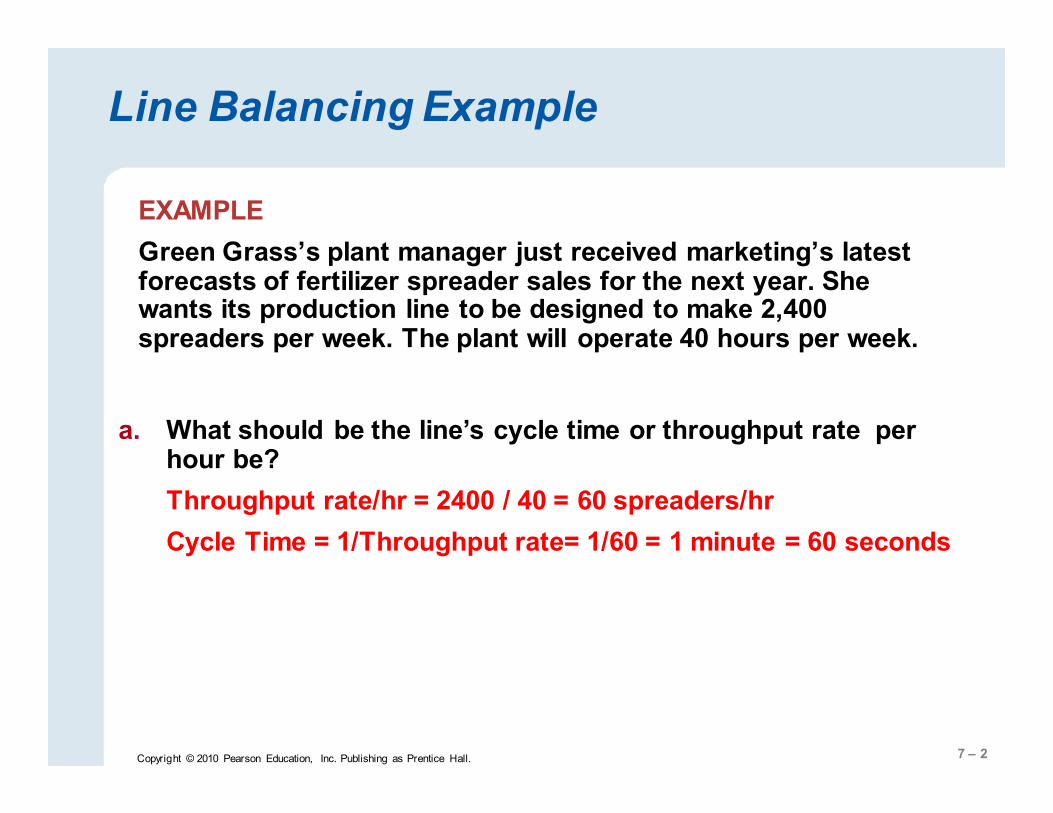
EXAMPLE

Green Grass’s plant manager just received marketing’s latest forecasts of fertilizer spreader sales for the next year. She wants its production line to be designed to make 2,400 spreaders per week. The plant will operate 40 hours per week.

a. What should be the line’s cycle time or throughput rate per hour be?

Throughput rate/hr = 2400 / 40 = 60 spreaders/hr

Cycle Time = 1/Throughput rate= 1/60 = 1 minute = 60 seconds


Line balancing Example continued:

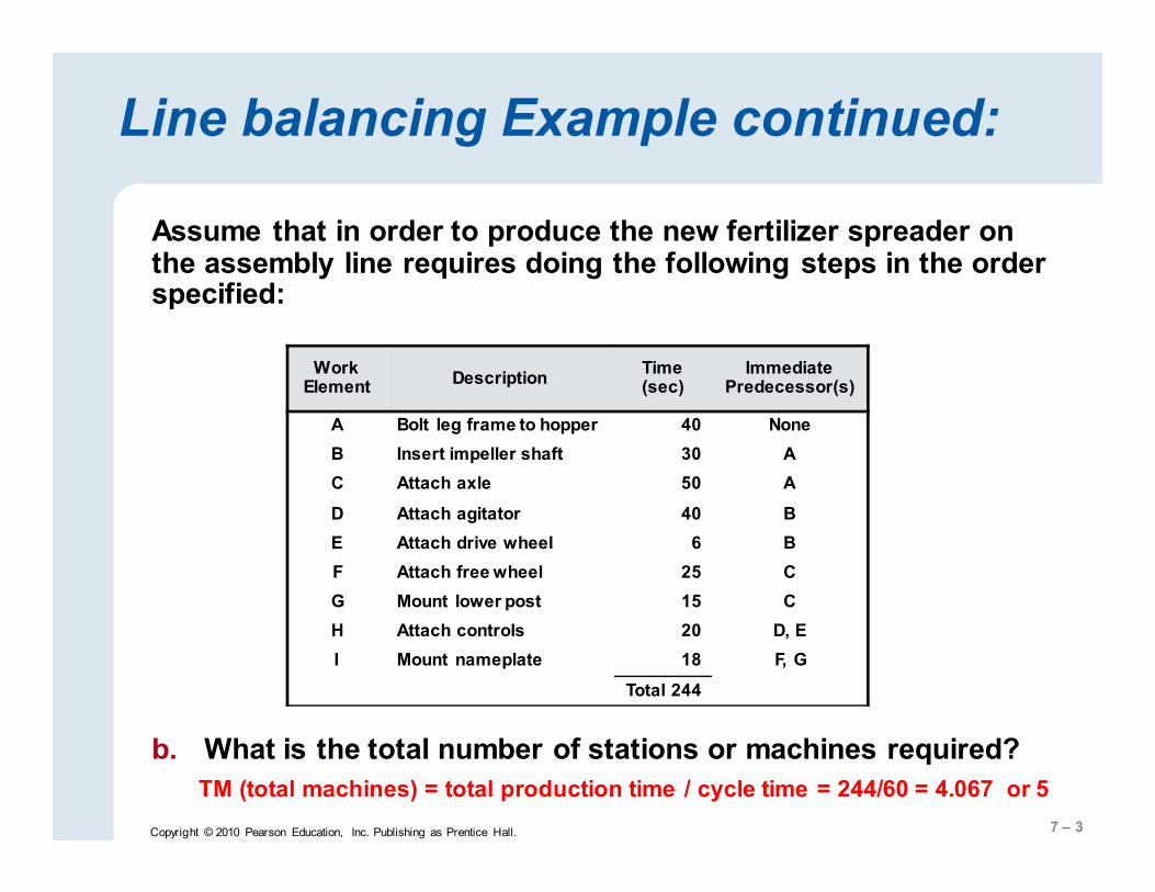
Assume that in order to produce the new fertilizer spreader on the assembly line requires doing the following steps in the order specified:

b. What is the total number of stations or machines required?

TM (total machines) = total production time / cycle time = 244/60 = 4.067 or 5

Work Element

Description Time (sec)

Immediate Predecessor(s)

A Bolt leg frame to hopper 40 None

B Insert impeller shaft 30 A

C Attach axle 50 A

D Attach agitator 40 B

E Attach drive wheel 6 B

F Attach free wheel 25 C

G Mount lower post 15 C

H Attach controls 20 D, E

I Mount nameplate 18 F, G

Total 244


Draw a Precedence Diagram

SOLUTION

The figure shows the complete diagram. We begin with work element A, which has no immediate predecessors. Next, we add elements B and C, for which element A is the only immediate predecessor. After entering time standards and arrows showing precedence, we add elements D and E, and so on. The diagram simplifies interpretation. Work element F, for example, can be done anywhere on the line after element C is completed. However, element I must await completion of elements F and G.

D

40

I

18

H

20

F

25

G

15

C

50

E

6

B

30

A

40

Precedence Diagram for Assembling the Big Broadcaster


Allocating work or activities to stations or machines

� The goal is to cluster the work elements into workstations so that

1. The number of workstations required is minimized

2. The precedence and cycle-time requirements are not violated

� The work content for each station is equal (or nearly so, but less than) the cycle time for the line

� Trial-and-error can be used but commercial software packages are also available


Finding a Solution

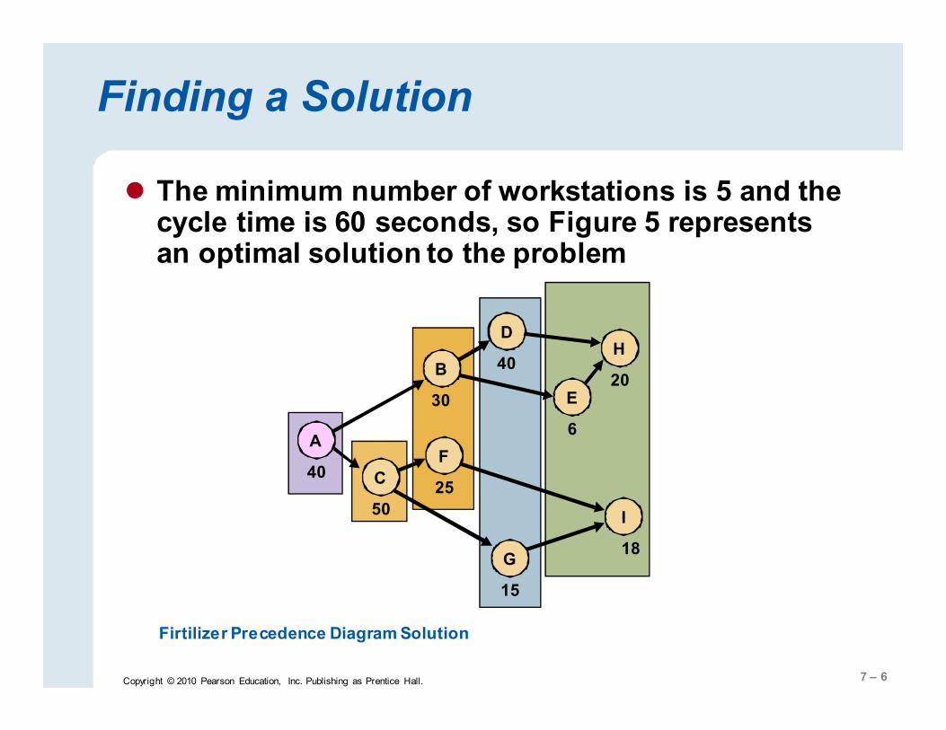
� The minimum number of workstations is 5 and the cycle time is 60 seconds, so Figure 5 represents an optimal solution to the problem

Firtilizer Precedence Diagram Solution

D

40

I

18

H

20

F

25 C

50

E

6

B

30

A

40

G

15


Calculating Line Efficiency

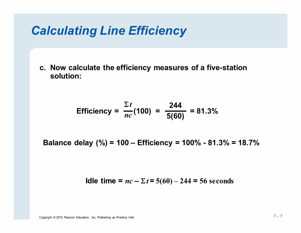
c. Now calculate the efficiency measures of a five-station solution:

Efficiency = (100) = ΣΣΣΣ t

nc

244

5(60) = 81.3%

Idle time = nc – ΣΣΣΣ t = 5(60) – 244 = 56 seconds

Balance delay (%) = 100 – Efficiency = 100% - 81.3% = 18.7%


A Line Process

� The desired output rate is matched to the staffing or production plan

� Line Cycle Time is the maximum time allowed for work at each station is

c = 1

r

where c = cycle time in hours r = desired output rate


A Line Process

� The theoretical minimum number of stations is

TM = ΣΣΣΣt

c

where

ΣΣΣΣt = total time required to assemble each unit


A Line Process

� Idle time, efficiency, and balance delay

Idle time = nc – ΣΣΣΣt

where

n = number of stations

Efficiency (%) = (100) ΣΣΣΣt

nc

Balance delay (%) = 100 – Efficiency


Solved Problem 2

A company is setting up an assembly line to produce 192 units per 8-hour shift. The following table identifies the work elements, times, and immediate predecessors:

Work Element Time (sec) Immediate Predecessor(s)

A 40 None

B 80 A

C 30 D, E, F

D 25 B

E 20 B

F 15 B

G 120 A

H 145 G

I 130 H

J 115 C, I

Total 720


Solved Problem 2

a. What is the desired cycle time (in seconds)?

b. What is the theoretical minimum number of stations?

c. Use trial and error to work out a solution, and show your solution on a precedence diagram.

d. What are the efficiency and balance delay of the solution found?

SOLUTION

a. Substituting in the cycle-time formula, we get

c = = 1

r

8 hours

192 units (3,600 sec/hr) = 150 sec/unit


Solved Problem 2

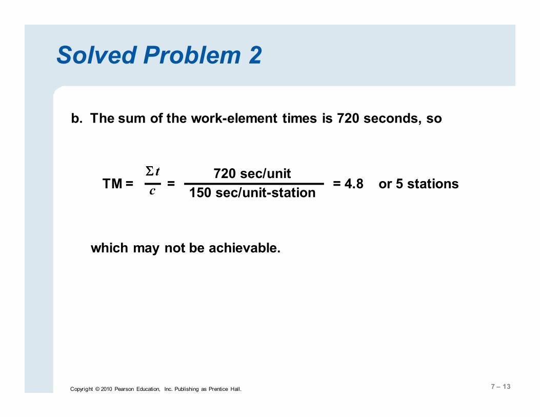
b. The sum of the work-element times is 720 seconds, so

TM = ΣΣΣΣ t

c = = 4.8 or 5 stations

720 sec/unit

150 sec/unit-station

which may not be achievable.


Solved Problem 2

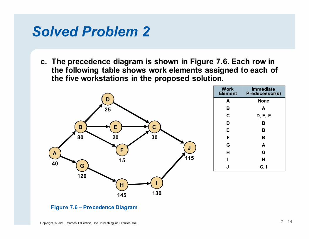
c. The precedence diagram is shown in Figure 7.6. Each row in the following table shows work elements assigned to each of the five workstations in the proposed solution.

J

115

C

30

D

25

E

20

F

15

I

130

H

145

B

80

G

120

A

40

Figure 7.6 – Precedence Diagram

Work Element

Immediate Predecessor(s)

A None

B A

C D, E, F

D B

E B

F B

G A

H G

I H

J C, I


Station Candidate(s) Choice Work-Element

Time (sec) Cumulative Time (sec)

Idle Time (c= 150 sec)

S1

S2

S3

S4

S5

Solved Problem 2

J

115

C

30

D

25

E

20

F

15 I

130 H

145

B

80

G

120

A

40


Solved Problem 2

J

115

C

30

D

25

E

20

F

15 I

130 H

145

B

80

G

120

A

40

A A 40 40 110

B B 80 120 30

D, E, F D 25 145 5

E, F, G G 120 120 30

E, F E 20 140 10

F, H H 145 145 5

F, I I 130 130 20

F F 15 145 5

C C 30 30 120

J J 115 145 5

Station Candidate(s) Choice Work-Element

Time (sec) Cumulative Time (sec)

Idle Time (c= 150 sec)

S1

S2

S3

S4

S5


Solved Problem 2

d. Calculating the efficiency, we get

Thus, the balance delay is only 4 percent (100–96).

Efficiency (%) = (100) ΣΣΣΣ t

nc =

720 sec/unit

5(150 sec/unit)

= 96%


In class - Example

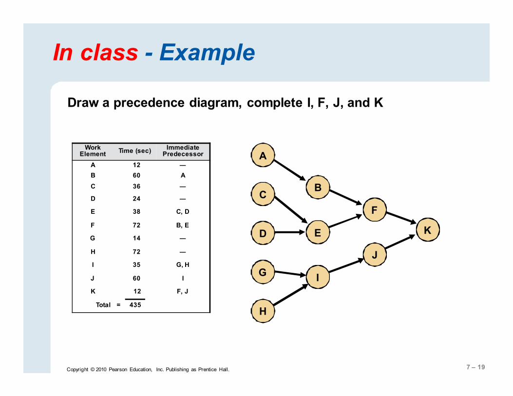
A plant manager needs a design for an assembly line to assembly a new product that is being introduced. The time requirements and immediate predecessors for the work elements are as follows:

Work Element Time (sec) Immediate

Predecessor

A 12 ―

B 60 A

C 36 ―

D 24 ―

E 38 C, D

F 72 B, E

G 14 ―

H 72 ―

I 35 G, H

J 60 I

K 12 F, J

Total = 435


K

In class - Example

Draw a precedence diagram, complete I, F, J, and K

Work Element

Time (sec) Immediate

Predecessor

A 12 ―

B 60 A

C 36 ―

D 24 ―

E 38 C, D

F 72 B, E

G 14 ―

H 72 ―

I 35 G, H

J 60 I

K 12 F, J

Total = 435

F

J

B

E

I

A

C

G

H

D


In class - Example

If the desired output rate is 30 units per hour, what are the cycle time and theoretical minimum?

c = = 1

r

1

30 (3600) = 120 sec/unit

TM = ΣΣΣΣ t

c = = 3.6 or 4 stations

435

120


In class - Example

Suppose that we are fortunate enough to find a solution with just four stations. What is the idle time per unit, efficiency, and the balance delay for this solution?

Idle time = nc – ΣΣΣΣ t

Efficiency (%) = (100) ΣΣΣΣ t

nc

Balance delay (%) = 100 – Efficiency

= 4(120) – 435 = 45 seconds

= 100 – 90.6 = 9.4%

= (100) = 90.6% 435

480


Station

Work Elements Assigned Cumulative Time

Idle Time (c = 120)

1

2

3

4

5

In class - Example

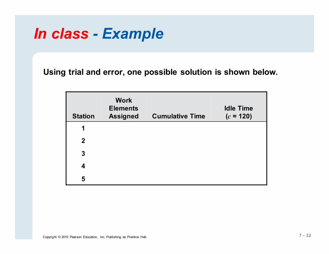
Using trial and error, one possible solution is shown below.


In class - Example

Using trial and error, one possible solution is shown below.

H, C, A 120 0

B, D, G 98 22

E, F 110 10

I, J, K 107 13

A fifth station is not needed

Station

Work Elements Assigned Cumulative Time

Idle Time (c = 120)

1

2

3

4

5


Managerial Considerations

� Pacing is the movement of product from one station to the next

� Behavioral factors such as absenteeism, turnover, and grievances can increase after installing production lines

� The number of models produced complicates scheduling and necessitates good communication

� Cycle times are dependent on the desired output rate

7 – 25

Inventory Management & the Economic Order Quantity (EOQ)

7 – 26

Lecture today

� Why is inventory so bad?

� Why hold inventory?

� Where to hold inventory?

� What are types of inventory to keep?

� What are the inventory costs?

� How much inventory to keep?

� When to order & how much to order?

� What do I need to know to make those decisions?

7 – 27

Inventory Management

� Inventory management is the planning and controlling of inventories in order to meet the competitive priorities of the organization.

� Inventory management requires information about expected demands, amounts on hand and amounts on order for every item stocked at all locations.

7 – 28

Inventory Basics

� Inventory is created when the receipt of materials, parts, or finished goods exceeds their disbursement.

� Inventory is depleted when their disbursement exceeds their receipt.

� An inventory manager’s job is to balance the advantages and disadvantages of both low and high inventories.

7 – 29

Inventory Costs

� Cost of capital

� Obsolescence

� Storage

� Insurance

� Taxes

� Security

� Theft

� Damage

� Locating

� Measurement

� Management & Labor

7 – 30

Why hold Inventory?

� Customer Sales & Service: Avoid Retail stock outs and thus customer goodwill (Retailing)

� Seasonal sales (Xmas trees)

� Take advantage of quantity discounts

� Balance process flow time

� Uncertainty in supply and demand

� Lead Time

� Speculative inventory (wine, gold)

7 – 31

Inventory at WAL-MART

� Making sure the shelves are stocked with tens of thousands of items at their 5,379 stores in 10 countries is no small matter for inventory managers at Wal-Mart.

� Knowing what is in stock, in what quantity, and where it is being held, is critical to effective inventory management.

� With inventories in excess of $29 billion, Wal-Mart is aware of the benefits from improved inventory management.

� They know that effective inventory management must include the entire supply chain.

� The firm is implementing radio frequency identification (RFID) technology in its supply chain.

7 – 32

7 – 33

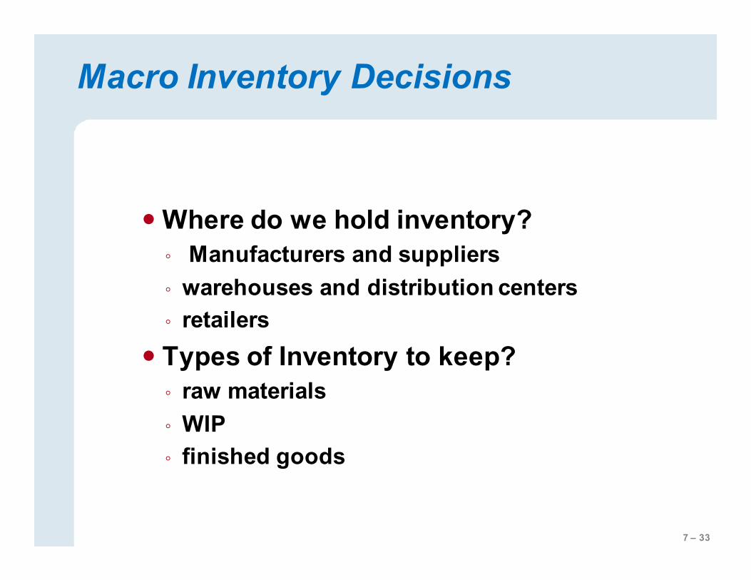
Macro Inventory Decisions

� Where do we hold inventory?

◦ Manufacturers and suppliers

◦ warehouses and distribution centers

◦ retailers

� Types of Inventory to keep?

◦ raw materials

◦ WIP

◦ finished goods

7 – 34

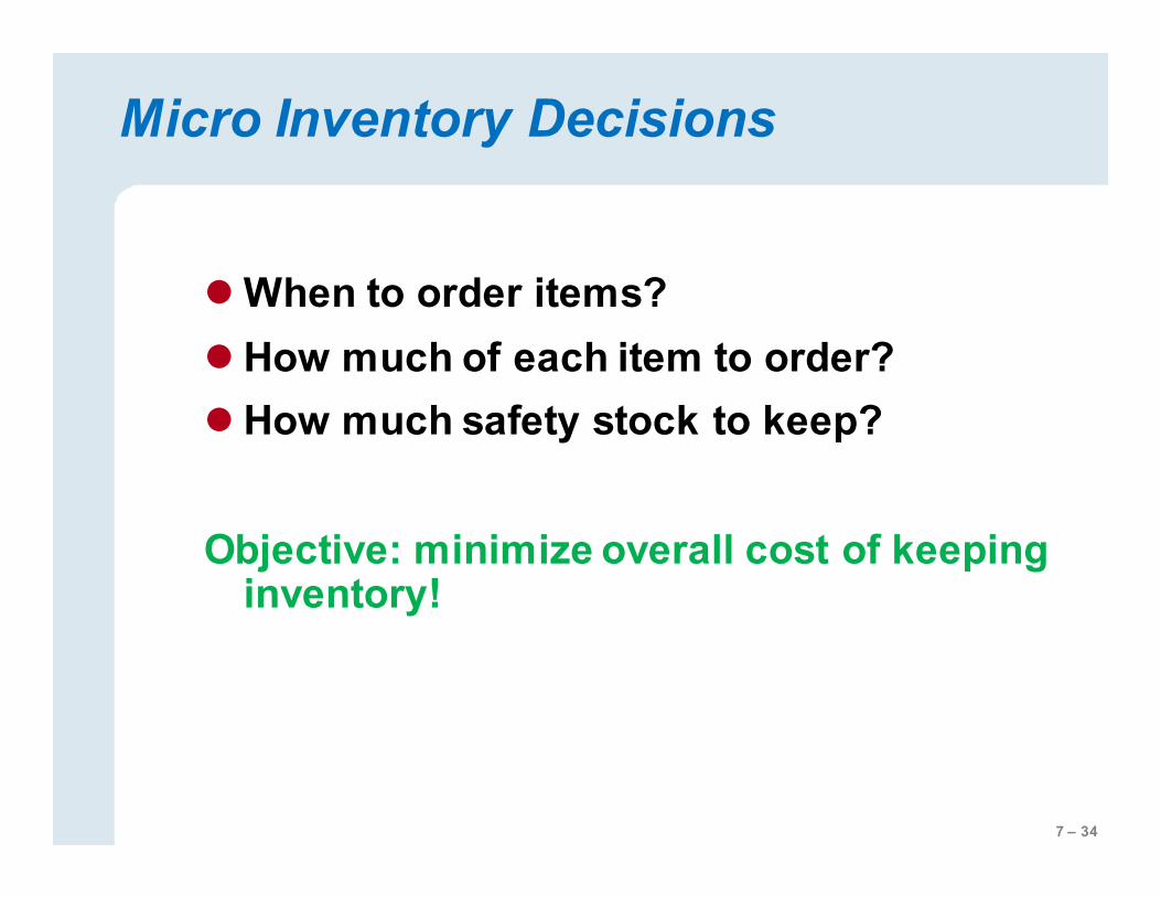
Micro Inventory Decisions

� When to order items?

� How much of each item to order?

� How much safety stock to keep?

Objective: minimize overall cost of keeping inventory!

7 – 35

Relevant Costs in an Inventory System

� Procurement costs

� Ordering cost (administrative, inspection, transportation etc.)

� Holding costs

� Maintenance and Handling

� Taxes

� Obsolescence

� Stock-outs costs

� Lost sales (Customer goodwill)

� Backorders

7 – 36

Relevant information to any inventory decision

� Knowing how much demand there is

� Knowing if this demand is fairly constant or varies

� Knowing what is in stock

� Knowing where they exist in the supply chain

� Knowing how long it will take to replenish

� Knowing where it is going to be replenished from

7 – 37

Frequently used inventory terms

� Inventory lot size

� Replenishment Lead time

� Stock out

� Reorder Point

� Safety stock

7 – 38

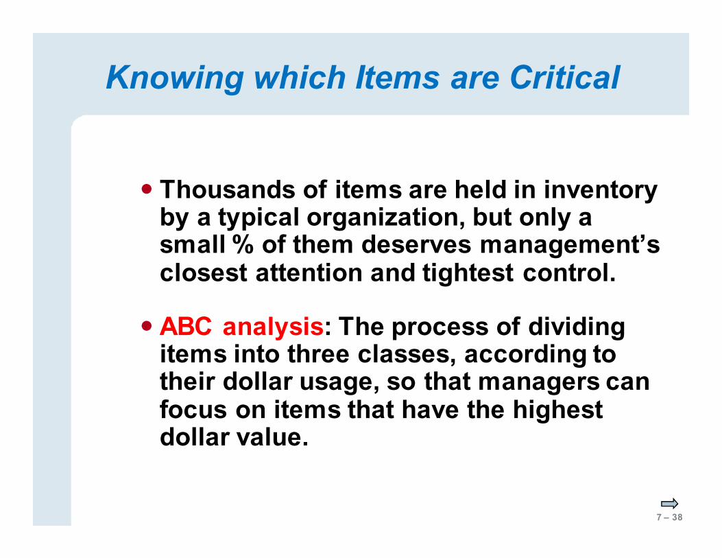
� Thousands of items are held in inventory by a typical organization, but only a small % of them deserves management’s closest attention and tightest control.

� ABC analysis: The process of dividing items into three classes, according to their dollar usage, so that managers can focus on items that have the highest dollar value.

Knowing which Items are Critical

7 – 39

ABC Analysis

10 20 30 40 50 60 70 80 90 100

Percentage of items

Pe

rce

nta

ge

of d

ollar

valu

e

100 —

90 —

80 —

70 —

60 —

50 —

40 —

30 —

20 —

10 —

0 —

Class C

Class A

Class B

7 – 40

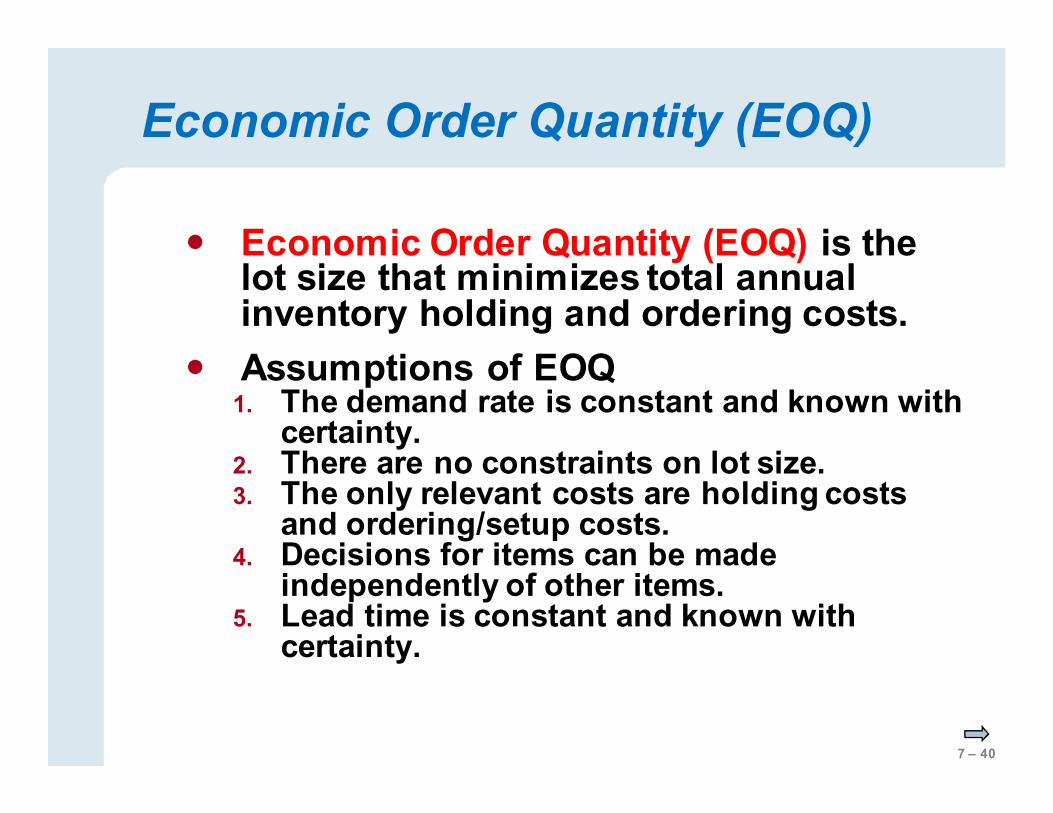
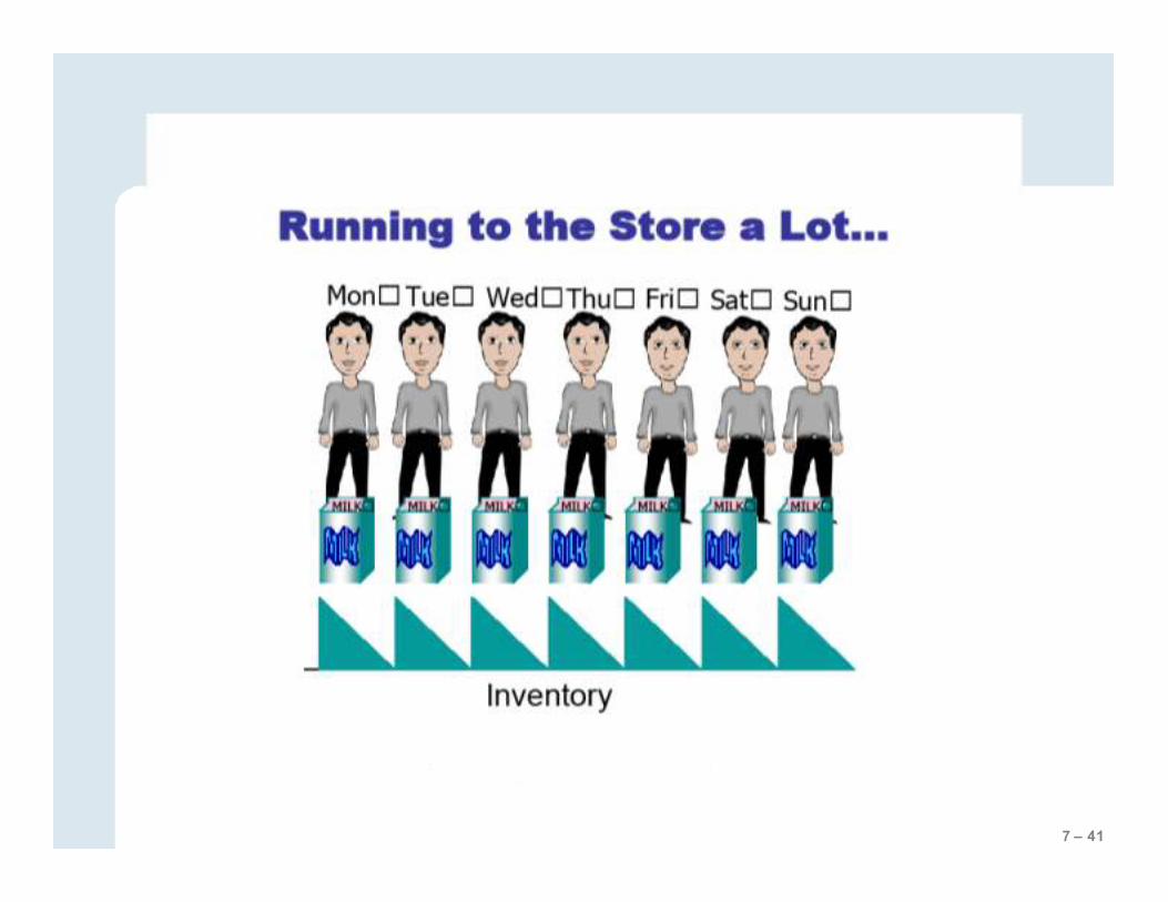
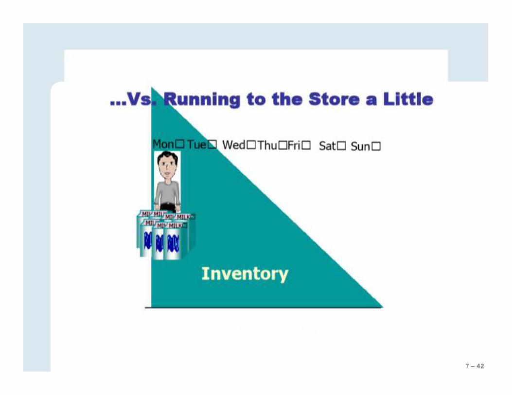
� Economic Order Quantity (EOQ) is the lot size that minimizes total annual inventory holding and ordering costs.

� Assumptions of EOQ 1. The demand rate is constant and known with

certainty. 2. There are no constraints on lot size. 3. The only relevant costs are holding costs

and ordering/setup costs. 4. Decisions for items can be made

independently of other items. 5. Lead time is constant and known with

certainty.

Economic Order Quantity (EOQ)

7 – 41

7 – 42

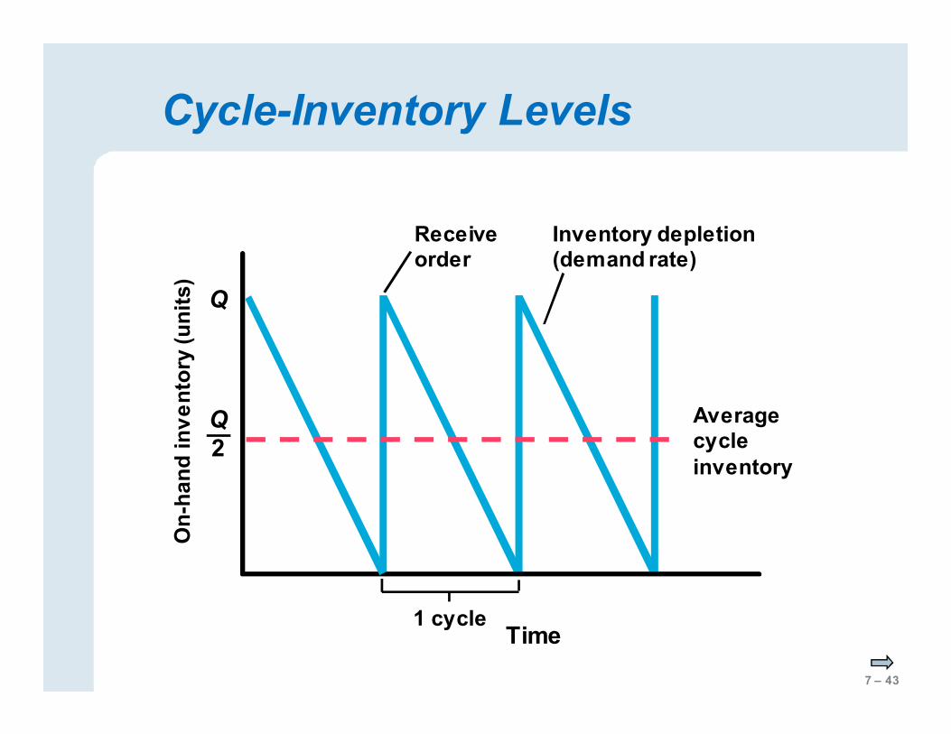
7 – 43

Inventory depletion (demand rate)

Receive order

1 cycle

On

-han

d in

ve

nto

ry (u

nit

s)

Time

Q

Average cycle inventory

Q — 2

Cycle-Inventory Levels

7 – 44

An

nu

al

co

st

(do

llars

)

Lot Size (Q)

Total Annual Cycle-Inventory Costs

Holding cost = (H) Q 2

Ordering cost = (S) D Q

Total cost = (H) + (S) D Q

Q 2

Q = lot size; C = total annual cycle-inventory cost H = holding cost per unit; D = annual demand S = ordering or setup costs per lot

7 – 45

Costing out a Lot Sizing Policy

� Bird feeder sales are 18 units per week, and the supplier charges $60 per unit. The cost of placing an order (S) with the supplier is $45.

� Annual holding cost (H) is 25% of a feeder’s value, based on operations 52 weeks per year.

� Management chose a 390-unit lot size (Q) so that new orders could be placed less frequently.

� What is the annual cycle-inventory cost (C) of the current policy of using a 390-unit lot size?

Museum of Natural History Gift Shop:

7 – 46

Costing out a Lot Sizing Policy

� What is the annual cycle-inventory cost (C) of the

current policy of using a 390-unit lot size?

D = (18 /week)(52 weeks) = 936 units H = 0.25 ($60/unit) = $15

C = $2925 + $108 = $3033

C = (H) + (S) = (15) + (45) Q

2

D Q

936 390

390

2

Museum of Natural History Gift Shop:

7 – 47

3000 —

2000 —

1000 —

0 — | | | | | | | |

50 100 150 200 250 300 350 400

Lot Size (Q)

Annual cost (d

olla

rs) Total cost

Holding cost

Ordering cost

Current cost

Current Q

Lowest cost

Best Q (EOQ)

Lot Sizing at the Museum of Natural History Gift Shop

7 – 48

Computing the EOQ

C = (H) + (S) Q

2

D Q

EOQ = 2DS H

D = annual demand S = ordering or setup costs per lot H = holding costs per unit

D = 936 units H = $15 S = $45

EOQ = 2(936)45

15 = 74.94 or 75 units

C = (15) + (45) 75

2 936 75

C = $1,124.10

Bird Feeders:

7 – 49

Time Between Orders

� Time between orders (TBO) is the average elapsed time between receiving (or placing) replenishment orders of Q units for a particular lot size.

� For the birdfeeder example, using an EOQ of 75 units.

TBOEOQ = EOQ D

TBOEOQ = = 75/936 = 0.080 year EOQ D

TBOEOQ = (75/936)(12) = 0.96 months

TBOEOQ = (75/936)(52) = 4.17 weeks

TBOEOQ = (75/936)(365) = 29.25 days

7 – 50

In Class Example

7 – 51

In Class Example

7 – 52

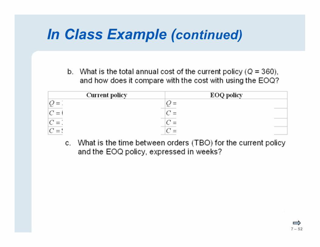
In Class Example (continued)

7 – 53

In Class Example continued

7 – 54

Understanding the Effect of Changes

� What happens if there is a change in the Demand Rate (D)?

� What happens if the Setup Costs (S) changes?

� What happens if the holding Costs (H) change?

� What happens if there are errors in estimating D, H, and S?

Documents

Line Balancing.. - libvolume8.xyzlibvolume8.xyz/textile/btech/semester7/industrialengineering/... · Line balancing Example continued: Assume that in order to produce the new fertilizer