Limit Load Analysis

8/3/2019 Limit Load Analysis

http://slidepdf.com/reader/full/limit-load-analysis 1/18

Problem 23

Limit load analysis of a pipebend



This page intentionally left blank.



Problem 23: Limit load analysis of a pipe bend

ADINA R & D, Inc. 23-1

Problem description

A pipe bend is subjected to a concentrated force as shown:

18

9

15 12

Displacement

gauge

P

x

y

Cross-section:0.432

6.625

All dimensions in inches.Material is stainless steel.

E = 29700 kpsi

n =0.27

The material of the pipe can be idealized as an elastic-plastic material using the von Mises

yield criterion with kinematic hardening, with the following points on the uniaxial stress-

strain curve:

Logarithmic strain True stress (103 psi)

6.06 × 10-4 18.0

0.002 35.40.0077 40.8

0.02 48.9

0.04 56.5

0.1 72.2




23-2 AUI Primer

We would like to obtain the force-deflection curve for the pipe and, in particular, the limit

load.

In this problem solution, we will demonstrate the following topics that have not been

presented in previous problems:

$Large displacement elastic-plastic analysis using shell elements.

$Specifying a collapse analysis.

$Adding text to the graphics window.

We assume that you have worked through problems 1 to 22, or have equivalent experience

with the AUI. Therefore we will not describe every user selection or button press.

Before you begin

Please refer to the Icon Locator Tables chapter of the Primer for the locations of all of the

AUI icons. Please refer to the Hints chapter of the Primer for useful hints.

This problem can be solved with the 900 nodes version of the ADINA System.

Invoking the AUI and choosing the finite element program

Invoke the AUI and choose ADINA Structures from the Program Module drop-down list.

Defining model control data

Problem heading: Choose Control→Heading, enter the heading AProblem 23: Limit load

analysis of a pipe bend@ and click OK.

Overall model control data: We will perform a collapse analysis using the load-displacement

control (LDC) algorithm to automatically choose the load step sizes. Choose Collapse

Analysis from the Analysis Type drop-down list. We will specify additional parameters

needed for the LDC algorithm later.

Kinematics: We anticipate that the displacements of the pipe can be large. Therefore we

select a large displacement, small strain formulation for use in the analysis. Choose

Control→Analysis Assumptions→Kinematics, set the Displacements/Rotations field to Large

and click OK.

Defining the model geometry

The diagram on the next page shows the key geometry used in defining the model:





P1 L1

L3

S1

S2

S3

P5P4

S4L5 L7

We will define the pipe midsurface by creating a circular cross-section at the base of the pipe

and then extruding the cross-section along the pipe axis.

To create the pipe cross-section, we will create a point on the pipe cross-section and revolve

the point around the pipe axis (at the base of the pipe, the pipe axis is coincident with the y-

axis). Click the Define Points icon , enter the following point and click OK.

Point # X1 X2 X3

1 -3.0965 0 0

(3.0965 corresponds to the radius of the midsurface of the pipe.) Now, to revolve the point,

click the Define Lines icon , add line number 1 and set the Type to Revolved. Set the

Initial Point to 1, the Angle of Rotation to 360, the Axis to Y and click OK. The graphics

window should look something like the figure on the next page.

Now we will extrude the cross-section in the direction of the y-axis to create the surface for

the first straight piece of the pipe. Click the Define Surfaces icon , add surface number 1

and set the Type to Extruded. Set the Initial Line to 1, the components of the Vector to 0.0,18.0, 0.0 and click OK.




23-4 AUI Primer

TIME 1.000

X Y

Z

We want to choose a more convenient view for the mesh plot. Click the Modify Mesh Plot

icon , click the View... button, set the View Direction (not the View Point) to 0.1, 0.1, 1.0,

set the Angle of Rotation to 135 and click OK twice to close both dialog boxes. The graphics

window should look something like the top figure on the next page.

We will display all successive meshes using this view, so we will change the default view.

Click the Save View icon .

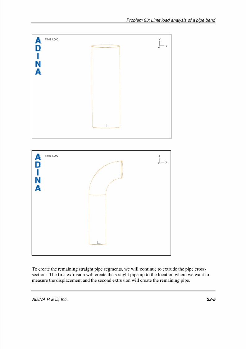
Let's continue the definition of the pipe surfaces. To create the pipe bend, we need to revolve

the newly-created cross-section line 90 degrees about an axis with center (9.0,18.0,0.0) and

components (0.0,0.0,1.0). From the mesh plot, we observe that the line that we need to

revolve is line number 3 (use the Query icon and the mouse to confirm this). Click the

Define Surfaces icon , add surface number 2 and set the Type to Revolved. Set the Initial

Line to 3, the Angle of Rotation to -90, “Axis of Revolution Defined by” to Vectors, the

components of the Vector Origin to 9, 18, 0 and the components of the Vector Direction to 0,

0, 1. When you click OK, the graphics window should look something like the bottom figure

on the next page. (You might need to use the mouse to rescale the mesh plot.)





TIME 1.000

X

Y

Z

TIME 1.000

X

Y

Z

To create the remaining straight pipe segments, we will continue to extrude the pipe cross-

section. The first extrusion will create the straight pipe up to the location where we want to

measure the displacement and the second extrusion will create the remaining pipe.




23-6 AUI Primer

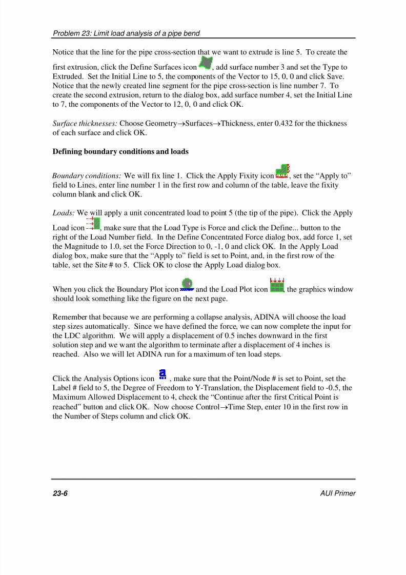
Notice that the line for the pipe cross-section that we want to extrude is line 5. To create the

first extrusion, click the Define Surfaces icon , add surface number 3 and set the Type to

Extruded. Set the Initial Line to 5, the components of the Vector to 15, 0, 0 and click Save.

Notice that the newly created line segment for the pipe cross-section is line number 7. To

create the second extrusion, return to the dialog box, add surface number 4, set the Initial Line

to 7, the components of the Vector to 12, 0, 0 and click OK.

Surface thicknesses: Choose Geometry→Surfaces→Thickness, enter 0.432 for the thickness

of each surface and click OK.

Defining boundary conditions and loads

Boundary conditions: We will fix line 1. Click the Apply Fixity icon , set the “Apply to”

field to Lines, enter line number 1 in the first row and column of the table, leave the fixity

column blank and click OK.

Loads: We will apply a unit concentrated load to point 5 (the tip of the pipe). Click the Apply

Load icon , make sure that the Load Type is Force and click the Define... button to the

right of the Load Number field. In the Define Concentrated Force dialog box, add force 1, set

the Magnitude to 1.0, set the Force Direction to 0, -1, 0 and click OK. In the Apply Load

dialog box, make sure that the “Apply to” field is set to Point, and, in the first row of the

table, set the Site # to 5. Click OK to close the Apply Load dialog box.

When you click the Boundary Plot icon and the Load Plot icon , the graphics window

should look something like the figure on the next page.

Remember that because we are performing a collapse analysis, ADINA will choose the load

step sizes automatically. Since we have defined the force, we can now complete the input for

the LDC algorithm. We will apply a displacement of 0.5 inches downward in the first

solution step and we want the algorithm to terminate after a displacement of 4 inches is

reached. Also we will let ADINA run for a maximum of ten load steps.

Click the Analysis Options icon , make sure that the Point/Node # is set to Point, set the

Label # field to 5, the Degree of Freedom to Y-Translation, the Displacement field to -0.5, the

Maximum Allowed Displacement to 4, check the “Continue after the first Critical Point is

reached” button and click OK. Now choose Control→Time Step, enter 10 in the first row in

the Number of Steps column and click OK.





B

U1

U2

U3 1 2 3

B - - - - - -

TIME 1.000

X

Y

Z

PRESCRIBEDFORCE

TIME 1.000

1.000

Defining the material

Click the Manage Materials icon and click the Plastic Multilinear button. In the Define

Multilinear Elastic-Plastic Material dialog box, add material 1, set the Young=s Modulus to

29700, the Poisson's ratio to 0.27 and the Type of Strain Hardening to Kinematic. Then enter

the following stress-strain data points in the Stress-Strain curve table (these points are

repeated from the problem description for convenience). Do not click OK yet.

Strain Stress

6.06E-04 18.0

0.002 35.4

0.0077 40.8

0.02 48.9

0.04 56.5

0.1 72.2

Now click the Graph button to display the stress-strain curve. The AUI displays a new

graphics window that should look something like the figure on the next page.




23-8 AUI Primer

0.

10.

20.

30.

40.

50.

60.

70.

80.

0.0 0.1

Uniaxial stress-strain curvesfrom material property data

Material 1,plastic-multilinear

(if large strain formulation used)

Logarithmic strain

T r u e

s t r e s s

Notice that the graph shows true stress vs logarithmic strain. For problems in which the

strains are relatively small, as in this problem, these quantities are close to the engineering

quantities.

Close the new graphics window, then click OK to close the Define Multilinear Elastic-Plastic

Material dialog box, and click Close to close the Manage Material Definitions dialog box.

Defining the finite elements and nodes

Element group control data: Click the Define Element Groups icon , add element group

1, set the Type to Shell and click OK.

Subdivision data: We enter the mesh size at the geometry points, with a smaller mesh size at

the pipe bend. First choose Meshing→Mesh Density→Complete Model, make sure that the

“Subdivision Mode” is “Use End-Point Sizes” and click OK. Now choose Meshing→

Mesh Density→Point Size, set the “Points Defined from” field to “All Geometry Points”, set

the Maximum to 4 and click Apply. Change the Mesh Size for points 2 and 3 to 2.0 and click

OK.

The graphics window should look something like the top figure on the next page.





B

U1

U2

U3 1 2 3

B - - - - - -

TIME 10.00

X

Y

Z

PRESCRIBEDFORCE

TIME 10.00

1.000

Finite elements: We will generate 9-node finite elements on the geometry surfaces. Click the

Mesh Surfaces icon , set the “Nodes per Element” to 9 and click the Options tab. In the

Nodal Coincidence Checking box, set the Check field to All Generated Nodes. Click the

Basic tab, enter surfaces 1, 2, 3, 4 in the first four rows of the table and click OK. The

graphics window should look something like this:

B

B B BB B B

U1

U2

U3 1 2 3

B - - - - - -

TIME 10.00

X

Y

Z

PRESCRIBEDFORCE

TIME 10.00

1.000




23-10 AUI Primer

Generating the ADINA data file, running ADINA, loading the porthole file

Click the Save icon and save the database to file prob23. Click the Data File/

Solution icon , set the file name to prob23, make sure that the Run Solution button is

checked and click Save. When ADINA is finished, close all open dialog boxes. Choose Post-Processing from the Program Module drop-down list and discard all changes. Then click the

Open icon , set the “Files of type” field to “ADINA-IN Database Files (*.idb)”, choose

file prob23 and click Open. Then click the Open icon and open porthole file prob23.

Please notice that we first opened the ADINA-IN database, then loaded the porthole file. We

did this so that we can create a force-deflection curve of the results using the geometry points.

Obtaining a deformed mesh plot

The graphics window should look something like this:

B

B B BB B B

U1

U2

U3 1 2 3

B - - - - - -

TIME 6.000

X

Y

Z

PRESCRIBEDFORCE

TIME 6.000

12.14

You will notice what appear to be missing lines in the finite element model. These lines lieon the outline (or silhouette) of the model. To display these lines, click the Modify Mesh Plot

icon and click the Rendering… button. In the Mesh Rendering Depiction dialog box, set

the “Generate Outline” field to “Geometry and Mesh”, then click OK twice to close both

dialog boxes.





Since we always want to display the outline lines in this model, click the Save Mesh Plot

Style icon .

(Note: the outline lines are only important if the mesh is relatively coarse and higher-order

elements are used, as in this model. So the default is for the outline lines not to be plotted.)

Obtaining a summary of model information

To view a summary of the model, choose List→Info→Model. There are 830 nodes and one

element group containing 210 shell elements. Click Close to close the dialog box.

To view a summary of loaded responses, choose List→Info→Response. There are seven load

steps loaded from times 0 to 6 (the first load step contains the initial conditions). Recall that

you requested 10 solution load steps; ADINA computed only 6 solution load steps because

the maximum displacement specified for collapse analysis was exceeded in step 6. Click

Close to close the dialog box.

Viewing the solutions

Use the Previous Solution icon and Next Solution icon to display the other solutions.

Notice that the deformations increase as the load increases, as we expect. When you are

finished, click the Last Solution icon .

Making a force-deflection curve graph

We will plot the applied force versus the deflection at the deflection gauge.

Result points: Before we can create the graph, we need to define result points for the node

where the load is applied and for the node associated with the displacement gauge. Since we

have geometry points at these node points, we will define these result points in terms of the

geometry points.

Choose Definitions→Model Point (Combination)→General, add name TIP, enter “POINT 5”

in the first row of the table and click Save. Define the name GAUGE to be the geometry

point 4 in the same way. Click OK to close the dialog box.

Variables: We need to define variables corresponding to the force and displacement. Choose

Definitions→Variable→Resultant, add resultant name FORCE, enter the expression

-<Y-PRESCRIBED_FORCE>

and click Save. Define the name DISP to be the expression




23-12 AUI Primer

-<Y-DISPLACEMENT>

in the same way. Click OK to close the dialog box.

Graph: Click the Clear icon , then choose Graph→Response Curve (Model Point). Set

the X variable to (User Defined:DISP) and set the X model point to GAUGE. Set the Yvariable to (User Defined:FORCE) and set the Y model point to TIP. Then click OK.

The graphics window should look something like this. It is, of course, possible to change the

graph title, axis labels and curve legends as was shown in problem 2.

0.

2.

4.

6.

8.

10.

12.

14.

0.0 0.5 1.0 1.5 2.0 2.5 3.0

RESPONSE GRAPH

No legend

DISP, GAUGE

F O R C E

, T

I P

Drawing bands of plastic strain

Let's draw bands corresponding to the accumulated effective plastic strain. This strain will

show us which areas of the pipe are most damaged.

Click the Clear icon , then the Mesh Plot icon .

In the band plots, we do not want to show the mesh geometry or the boundary conditions.

Click the Show Geometry icon and the Boundary Plot icon . Then click the Save

Mesh Plot Style icon to update the defaults.





To draw the bands, click the Create Band Plot icon , set the Band Plot Variable to (Strain:

ACCUM_EFF_PLASTIC_STRAIN) and click OK. Use the Pick icon and the mouse to

resize the mesh plot and rearrange the annotations until the graphics window looks something

like this:

TIME 6.000

X

Y

Z

ACCUMEFFPLASTICSTRAIN

RST CALC

SHELL T = 1.00

TIME 6.000

0.03000

0.02333

0.016670.01000

0.00333

-0.00333

-0.01000

MAXIMUM0.03278

EG 1, EL 115, IPT 132 (0.02319)

MINIMUM-0.01165

EG 1, EL 113, IPT 132 (0.002253)

We are now observing the plastic strains on the top surface of the pipe skin (which is the outer

surface in this model). We would also like to observe the plastic strains on the bottom (inner)surface of the pipe skin. So we will display another mesh plot, then we will plot plastic

strains of the inner surface onto this mesh plot.

Click the Mesh Plot icon and use the Pick icon to move the mesh plot to a position

under and to the right of the first mesh plot. Shrink both mesh plots so that they both fit in the

graphics window. Also delete any duplicate text and axes. The graphics window should look

something like the figure on the next page.

Now, before we draw the bands on the second mesh plot, we instruct the AUI to compute

plastic strains on the bottom surface of the shell elements. Choose Definitions→ResultControl, set the Result Control Name to DEFAULT, set the t Coordinate field to -1.0 and

click OK. Click the Create Band Plot icon , set the Band Plot Variable to (Strain:

ACCUM_EFF_PLASTIC_STRAIN) and click OK.




23-14 AUI Primer

TIME 6.000

X

Y

Z


RST CALC

SHELL T = 1.00

TIME 6.000

0.03000

0.02333

0.01667

0.01000

0.00333

-0.00333

-0.01000

MAXIMUM0.03278

EG 1, EL 115, IPT 132 (0.02319)

MINIMUM

-0.01165EG 1, EL 113, IPT 132 (0.002253)

TIME 6.000

X

Y

Z

It is difficult to compare the two pictures because the band tables are different. So we will use

the same band table for both band plots. Click the Modify Band Plot icon , set the Band

Plot Name to BANDPLOT00001, click the Band Table... button, set the Value Range to 0.0

and 0.04 and click OK twice to close both dialog boxes. Repeat this procedure for band plot

BANDPLOT00002.

We are also not interested in the minimum value of the plastic strain. Click the Modify Band

Plot icon , set the Band Plot Name to BANDPLOT00001, click the Band Rendering...

button, set the “Extreme Values” field to “Plot the Maximum” and click OK twice to close

both dialog boxes. Repeat this procedure for band plot BANDPLOT00002.

Since we now have two band tables, each with almost the same information, use the Pick icon

and the mouse to delete one of them.

Let's add some text to label the two plots. Choose Display→Text→Draw, enter the text

Outer surface

in the Text box and click OK. The AUI draws the text near the center of the graphics

window. Use the Pick icon to move and resize the text so that it is below the base of the

upper mesh plot. Repeat these steps for the text

Inner surface





and place this text below the base of the lower mesh plot.

The graphics window should look something like this:

TIME 6.000

X

Y

Z

TIME 6.000

X

Y

Z


RST CALC

SHELL T = 1.00

TIME 6.000

0.03900

0.03300

0.02700

0.02100

0.01500

0.009000.00300

MAXIMUM0.03278

EG 1, EL 115, IPT 132 (0.02319)

MAXIMUM0.04833

EG 1, EL 108, IPT 311 (0.03232)

Outer surface

Inner surface

Exiting the AUI: Choose File→Exit to exit the AUI. You can discard all changes.




23 16 AUI Primer

This page intentionally left blank

Documents

Limit Load Analysis