Limit cycleʼs uniqueness for second order ODEʼs polynomial in

J. Math. Anal. Appl. 381 (2011) 402–413

Contents lists available at ScienceDirect

Journal of Mathematical Analysis andApplications

www.elsevier.com/locate/jmaa

Limit cycle’s uniqueness for second order ODE’s polynomial in x

M. Sabatini ∗

Dip. di Matematica, Univ. di Trento, I-38050 Povo (TN), Italy

a r t i c l e i n f o a b s t r a c t

Article history:Received 9 November 2010Available online 22 February 2011Submitted by Steven G. Krantz

Keywords:UniquenessLimit cycleSecond order ODEsMassera theoremConti–Filippov transformation

We prove a uniqueness result for limit cycles of the second order ODE x + ∑ Jj=1 f j(x)x j +

g(x) = 0. We extend a uniqueness result proved in Carletti, Rosati and Villari (2007) [2].The main tool applied is an extension of the Massera theorem proved in Guillamon andSabatini (2007) [5].

© 2011 Elsevier Inc. All rights reserved.

1. Introduction

In this paper we are concerned with planar differential systems of the form

x = y, y = −g(x) −J∑

j=1

f j(x)y j, (1)

equivalent to the second order differential equations of the form

x +J∑

j=1

f j(x)x j + g(x) = 0. (2)

Several mathematical models of physics, economics, biology are governed by second order differential equations [3,8,10].Other models can be reduced to systems of the type (1) by means of suitable transformations. The asymptotic behaviourof their solutions is one of the main objects of study. In this perspective, the existence of special solutions as stationaryones, or isolated cycles, is of primary interest. This is particularly true if such solutions attract (repel) neighbouring ones,so that the system’s dynamics is dominated by that of the attracting equilibria or cycles. In the special case of an isolatedcycle attracting all the other solutions but equilibria, the description of the system’s dynamics becomes quite simple, sincethe asymptotic behaviour of all solutions but the equilibrium one is just that of the limit cycle. Uniqueness theorems forlimit cycles have been extensively studied (see [2,11,12,4] for recent results and extensive bibliographies [13, Chapter IV,Section 4]). In general, studying the number and location of limit cycles is a non-trivial problem, as shown by the resistanceof the Hilbert XVI problem. Such a problem has been recently re-proposed as a main research problem (see [9, Problem 13]).A strictly related subject is that of hyperbolicity. A T -periodic cycle γ (t) of a differential system

* Fax: +39(0461)881624.E-mail address: [email protected].

0022-247X/$ – see front matter © 2011 Elsevier Inc. All rights reserved.doi:10.1016/j.jmaa.2011.02.055

http://dx.doi.org/10.1016/j.jmaa.2011.02.055

http://www.ScienceDirect.com/

http://www.elsevier.com/locate/jmaa

mailto:[email protected]

http://dx.doi.org/10.1016/j.jmaa.2011.02.055

M. Sabatini / J. Math. Anal. Appl. 381 (2011) 402–413 403

x = P (x, y), y = Q (x, y), (3)

is said to be hyperbolic if

T∫0

div(γ (t)

)dt �= 0, (4)

where div = ∂ P∂x + ∂ Q

∂ y is the divergence of (3). Hyperbolicity plays a main role in perturbation problems, since smoothperturbations of hyperbolic cycles do not allow multiple bifurcations. An attractive cycle is not necessarily hyperbolic.

Most of the uniqueness results proved for planar systems are concerned with the classical Liénard system and its gener-alizations, such as

x = ξ(x)[ϕ(y) − F (x)

], y = −ζ(y)g(x), ξ(x) �= 0, ζ(y) �= 0. (5)

Such a class of systems also contains Lotka–Volterra systems and systems equivalent to the Rayleigh equation as specialcases [3]. Such systems are characterized by the presence, both in x and y, of a single mixed term obtained as the productof single-variable functions, resp. ξ(x)ϕ(y) and ζ(y)g(x). Moreover, such systems can be easily transformed into the systemswithout mixed terms, by applying the transformation

X(x) =x∫

0

1

ξ(s)ds, Y (y) =

y∫0

1

ζ(s)ds.

The transformed system has the form

X = ϕ(Y ) − F (X), y = g(X),

for suitable functions ϕ(Y ), F (X), g(X).In order to study the systems with several distinct mixed terms, a different approach is required. Some recent results

[2,4] are concerned with the following systems,

x = y, y = −x − yN∑

k=0

f2k+1(x)y2k, (6)

equivalent to the equations

x +N∑

k=0

f2k+1(x)x2k+1 + x = 0. (7)

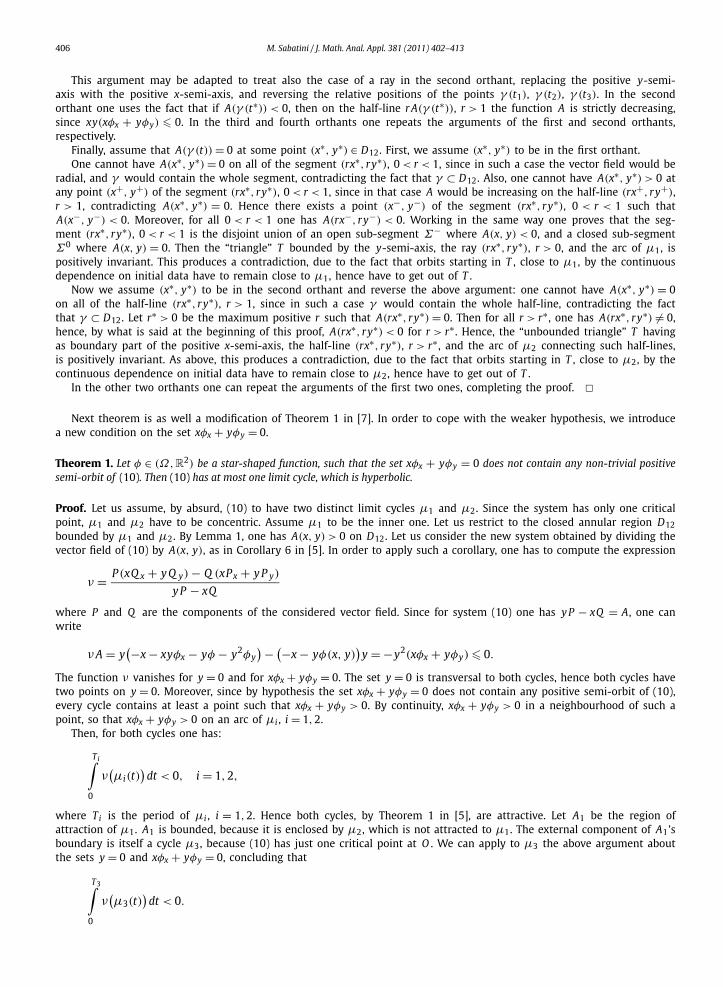
Such systems cannot be reduced to the form (5) by the above transformation. In order to prove the limit cycle uniqueness,the authors extend a classical result by Massera about the uniqueness and global (except for equilibria) attractiveness ofLiénard limit cycles [6]. Such a result comes from the two main properties. The first one is that every cycle be star-shaped,fact proved in a new way in [2]. The second one is that the vector field rotates clockwise along the rays (half-lines havingextreme at the axes’ origin O ). In fact, in general such properties are not sufficient to prove the limit cycle’s uniqueness, asthe following example shows,{

x = y(x2 + y2 − (

x2 + y2)2) + x

(1 − 3

(x2 + y2

) + (x2 + y2

)2),

y = −x(x2 + y2 − (

x2 + y2)2) + y

(1 − 3

(x2 + y2

) + (x2 + y2

)2).

(8)

Such a system has two star-shaped limit cycles coinciding with the circles x2 + y2 = 3−√5

2 and x2 + y2 = 3+√5

2 . The internalone is an attractor, the external one is a repellor. The vector field rotates clockwise along every ray (see Fig. 1).

An even more pathological example (from the point of view of the Massera-like theorems) is the system

x = y cos(x2 + y2) − x sin

(x2 + y2), y = −x cos

(x2 + y2) − y sin

(x2 + y2). (9)

Such a system satisfies both properties, and has infinitely many cycles coinciding with the circles {x2 + y2 = kπ : k ∈ N}.Such cycles are alternatively repelling and attracting, and rotate alternatively counter-clockwise and clockwise. A cycle’sattraction (repulsion) region is the annular region bounded by the two adjacent limit cycles, except for the innermost one,whose attraction region has the origin in its boundary.

As a consequence, an additional condition is required in order to give a complete proof of a Massera-like theorem.Corollary 6 of [5] provides a natural additional condition, asking for the angular velocity not to vanish in the whole plane.The same result can be proved if the angular velocity does not vanish in a suitable subregion of the plane, as in [7].

404 M. Sabatini / J. Math. Anal. Appl. 381 (2011) 402–413

Fig. 1. The system (8) has two limit cycles.

Corollary 6 is a particular case of Theorem 2 in [5], a rather general extension to the Massera theorem. In such a theoreman auxiliary function ν is used in order to study the cycles’ hyperbolicity. The main property of ν is that its integral on acycle coincides with that of the vector field’s divergence. On the other hand, ν has an advantage over the divergence, sinceit can be everywhere negative in presence of a repelling critical point and an attracting limit cycle, while in such a situationthe divergence has to change the sign. This helps in proving the limit cycle’s uniqueness, as in [7]. Additionally, Theorem 2in [5] allows to prove the limit cycle’s hyperbolicity, which is not a consequence of the Massera-like theorems.

In this paper we extend in two ways the uniqueness result of [2]. First, we consider the systems with even degree termsf2k(x)y2k , then we allow g(x) to be non-linear, provided xg(x) �= 0 for x �= 0 in some interval. Even degree terms can betreated by considering the function

∑ Jj=1 f j(x)y j−1 as the sum of y-trinomials, each satisfying suitable conditions. On the

other hand, considering a non-linear g(x) allows to work in different regions for the same system. Since an x-translationtransforms a system of the form (1) into a system of the same form, one just has to translate a critical point to the origin,proving the uniqueness, in a suitable strip (a,b) × R, of limit cycles surrounding such a point.

If the system has the form (6), with g(x) = x, our result extends that one obtained in [2], replacing the sign and mono-tonicity conditions on f2k+1(x) with a monotonicity condition on x2k f2k+1(x). This allows to apply our theorem to somepolynomial coefficients, as f3(x) = x4 − x2 + 1, which do not satisfy the hypotheses in [2].

In order to extend the results of [2], we follow a different approach w.r. to that one developed in [7]. We cannot applyTheorem 1 of [7] to (6), since φ(x, y) = ∑N

k=0 f2k+1(x)y2k does not satisfy the strict star-shapedness condition requiredby such a theorem. In order to overcome such an obstacle we introduce a non-invariance property similar to that oneappearing in the LaSalle Invariance Principle. In fact, the passage from xφx + yφy > 0 to xφx + yφy � 0 is analogous to thepassage from the condition V < 0 to the condition V � 0 in studying asymptotic stability problems. Moreover, rather thanjust proving the cycle’s star-shapedness, we prove that, assuming by absurd the existence of two concentric limit cycles,then there exists an annular region containing both ones, where the angular velocity does not vanish. This allows to applyTheorem 2 in [5] in order to get the limit cycle’s uniqueness and its hyperbolicity.

Our paper is organized as follows. In Section 2 we prove the main theorem about uniqueness and hyperbolicity forsystems with a linear g(x). Then we apply such a theorem to some special cases.

In Section 3 we apply the Conti–Filippov transformation in order to reduce a system of the form (1) with a non-linearg(x) to another system of the same type, but with a linear g(x). In this section we derive the uniqueness condition in strips.

In both sections we also consider the question of limit cycles existence, giving sufficient conditions for the solutions’boundedness that allow to apply the Poincaré–Bendixson theorem.

2. g(x) linear

Since our approach is based on the cycle’s star-shapedness, we restrict to a star-shaped subset Ω ⊂ R2. In this context,

we think of Ω as a strip (a,b) × R, with a < 0 < b, but what follows holds for arbitrary star-shaped subsets. We denotepartial derivatives by subscripts, i.e. φx is the derivative of φ w.r. to x, etc. We say that a function φ ∈ C1(Ω,R) is star-shaped if (x, y) · ∇φ = xφx + yφy does not change the sign. We say that φ is strictly star-shaped if (x, y) · ∇φ �= 0, except atthe origin O = (0,0). We call ray a half-line having origin at the point (0,0). We denote by γ (t, x, y) the unique solutionof the system (1) such that γ (0, x, y) = (x, y). For definitions related to dynamical systems, we refer to [1].


Throughout all of this paper we assume the system (1) to satisfy some hypotheses ensuring existence and uniqueness ofsolutions, and continuous dependence on initial data. This occurs if, for instance, one has

•) f j , j = 1, . . . , J , continuous on their domains;•) g Lipschitzian on its domain.

In this section we are concerned with the system (1), assuming g(x) = kx. Without loss of generality, possibly performinga time rescaling, we may restrict to the case k = 1. In this case, we may consider (1) as a special case of a more generalclass of systems,

x = y, y = −x − yφ(x, y). (10)

We first consider a sufficient condition for limit cycle’s uniqueness. It has the same form as system (9) in [7], but here thefunction φ(x, y) is not strictly star-shaped. This will force us to modify the proof in the part related to the angular velocity,and add a hypothesis in the main theorem. As in [7], we set

A(x, y) = yx − xy = y2 + x2 + xyφ(x, y).

The sign of A(x, y) is opposite to that of the angular speed of the solutions of (10). In general, A(x, y) changes sign alongthe solutions of (10), even in the simplest example of the non-linear Liénard system with a limit cycle

x = y, y = −x − y(x2 − 1

). (11)

In fact, the orbits of (11) approaching the limit cycle from the second and fourth orthants change angular velocity whenthey get closer to the limit cycle.

Our uniqueness result comes from Theorem 2 of [5], in the form of Corollary 6. In the following lemma we prove thatif two limit cycles μ1 and μ2 exist, then in the closed annular region D12 bounded by μ1 and μ2 the function A does notvanish. The next lemma’s proof is a modification of part of the proof of Theorem 1 in [7]. We emphasize that we consideropen orthants, i.e. orthants without semi-axes.

Lemma 1. Let φ ∈ C1(Ω,R2), with xφx + yφy � 0 in Ω . If the system (10) has two distinct limit cycles μ1 and μ2 , then A(x, y) > 0

on D12 .

Proof. The system (10) has one critical point, hence μ1 and μ2 are concentric. Let μ1 be the inner one, μ2 be the outerone. The radial derivative Ar of A is given by

Ar = xAx + y A y

r= 1

r

(2A + xy(xφx + yφy)

) = 1

r(2A + xyrφr).

Hence the function A satisfies the differential equation r Ar = 2A +xy(xφx + yφy), whose right-hand side sign determines themonotonicity of A along the rays. If x∗ y∗ > 0 and A(x∗, y∗) > 0, then Ar > 0 at (x∗, y∗) and at every point (rx∗, ry∗) withr > 1, hence A is strictly increasing on the half-line {(rx∗, ry∗): r > 1}. On the other hand, if x∗ y∗ < 0 and A(x∗, y∗) < 0,then Ar < 0 at (x∗, y∗) and at every point (rx∗, ry∗) with r > 1, hence A is strictly decreasing on the half-line {(rx∗, ry∗): r >

1}.If A(x∗, y∗) = 0 and x∗ y∗ > 0, then either A(rx∗, ry∗) = 0 for all r > 1, or at some point of the half-line {(rx∗, ry∗): r > 1}

the radial derivative Ar becomes positive, so that A(rx∗, ry∗) > 0 for all r > r, for some r > 1.Similarly, if A(x∗, y∗) = 0 and x∗ y∗ < 0, then either A(rx∗, ry∗) = 0 for all r > 1, or at some point of the half-line

{(rx∗, ry∗): r > 1} the radial derivative Ar becomes negative, so that A(rx∗, ry∗) < 0 for all r > r, for some r > 1.We prove that, for every orbit γ contained in D12, A(γ (t)) > 0. Every orbit in D12 meets every semi-axis, otherwise

its positive limit set would contain a critical point different from O . On every semi-axis one has A(x, y) > 0. Assumefirst, by absurd, A(γ (t)) to change sign. Then there exist t1 < t2 such that A(γ (t1)) > 0, A(γ (t2)) < 0, and γ (ti), i = 1,2are on the same ray. Assume γ (ti), i = 1,2 to be in the first orthant. Two cases can occur: either |γ (t1)| < |γ (t2)| or|γ (t1)| > |γ (t2)|. The former, |γ (t1)| < |γ (t2)|, contradicts the fact that A is radially increasing in the first orthant, henceone has |γ (t1)| > |γ (t2)|. The orbit γ crosses the segment Σ = {rγ (t1), 0 < r < 1} at γ (t2), going towards the positivey-semi-axis. Let G be the sub-region of the first orthant bounded by the positive y-semi-axis, the ray {rγ (t1), r > 0} andthe portions of μ1, μ2 meeting the y-axis and such a ray. The orbit γ cannot remain in G , since in that case G wouldcontain a critical point different from O . Also, γ cannot leave G crossing the positive y-semi-axis, because A(x, y) > 0 onsuch an axis. Hence γ leaves G passing again through the segment Σ . That implies the existence of t3 > t2, such that γ (t3)

lies on the ray {rγ (t1), 0 < r}. Again, one cannot have |γ (t3)| < |γ (t2)|, since A(γ (t3)) > 0 implies A increasing on thehalf-line rγ (t3), r > 1, hence one has |γ (t3)| > |γ (t2)|. Also, one cannot have |γ (t3)| < |γ (t1)|, otherwise γ would entera positively invariant region, bounded by the curve γ (t), for t1 � t � t3, and by the segment with extrema γ (t1), γ (t3),hence there would exist a critical point different from O . As a consequence, one has |γ (t3)| > |γ (t1)|. Since A(x, y) > 0 onthe segment joining γ (t1) and γ (t3), such a segment, with the portion of orbit joining γ (t1) and γ (t3) bounds a regionwhich is negatively invariant for (10), hence contains a critical point different from O , contradiction.


This argument may be adapted to treat also the case of a ray in the second orthant, replacing the positive y-semi-axis with the positive x-semi-axis, and reversing the relative positions of the points γ (t1), γ (t2), γ (t3). In the secondorthant one uses the fact that if A(γ (t∗)) < 0, then on the half-line r A(γ (t∗)), r > 1 the function A is strictly decreasing,since xy(xφx + yφy) � 0. In the third and fourth orthants one repeats the arguments of the first and second orthants,respectively.

Finally, assume that A(γ (t)) = 0 at some point (x∗, y∗) ∈ D12. First, we assume (x∗, y∗) to be in the first orthant.One cannot have A(x∗, y∗) = 0 on all of the segment (rx∗, ry∗), 0 < r < 1, since in such a case the vector field would be

radial, and γ would contain the whole segment, contradicting the fact that γ ⊂ D12. Also, one cannot have A(x∗, y∗) > 0 atany point (x+, y+) of the segment (rx∗, ry∗), 0 < r < 1, since in that case A would be increasing on the half-line (rx+, ry+),r > 1, contradicting A(x∗, y∗) = 0. Hence there exists a point (x−, y−) of the segment (rx∗, ry∗), 0 < r < 1 such thatA(x−, y−) < 0. Moreover, for all 0 < r < 1 one has A(rx−, ry−) < 0. Working in the same way one proves that the seg-ment (rx∗, ry∗), 0 < r < 1 is the disjoint union of an open sub-segment Σ− where A(x, y) < 0, and a closed sub-segmentΣ0 where A(x, y) = 0. Then the “triangle” T bounded by the y-semi-axis, the ray (rx∗, ry∗), r > 0, and the arc of μ1, ispositively invariant. This produces a contradiction, due to the fact that orbits starting in T , close to μ1, by the continuousdependence on initial data have to remain close to μ1, hence have to get out of T .

Now we assume (x∗, y∗) to be in the second orthant and reverse the above argument: one cannot have A(x∗, y∗) = 0on all of the half-line (rx∗, ry∗), r > 1, since in such a case γ would contain the whole half-line, contradicting the factthat γ ⊂ D12. Let r∗ > 0 be the maximum positive r such that A(rx∗, ry∗) = 0. Then for all r > r∗ , one has A(rx∗, ry∗) �= 0,hence, by what is said at the beginning of this proof, A(rx∗, ry∗) < 0 for r > r∗ . Hence, the “unbounded triangle” T havingas boundary part of the positive x-semi-axis, the half-line (rx∗, ry∗), r > r∗ , and the arc of μ2 connecting such half-lines,is positively invariant. As above, this produces a contradiction, due to the fact that orbits starting in T , close to μ2, by thecontinuous dependence on initial data have to remain close to μ2, hence have to get out of T .

In the other two orthants one can repeat the arguments of the first two ones, completing the proof. �Next theorem is as well a modification of Theorem 1 in [7]. In order to cope with the weaker hypothesis, we introduce

a new condition on the set xφx + yφy = 0.

Theorem 1. Let φ ∈ (Ω,R2) be a star-shaped function, such that the set xφx + yφy = 0 does not contain any non-trivial positive

semi-orbit of (10). Then (10) has at most one limit cycle, which is hyperbolic.

Proof. Let us assume, by absurd, (10) to have two distinct limit cycles μ1 and μ2. Since the system has only one criticalpoint, μ1 and μ2 have to be concentric. Assume μ1 to be the inner one. Let us restrict to the closed annular region D12bounded by μ1 and μ2. By Lemma 1, one has A(x, y) > 0 on D12. Let us consider the new system obtained by dividing thevector field of (10) by A(x, y), as in Corollary 6 in [5]. In order to apply such a corollary, one has to compute the expression

ν = P (xQ x + y Q y) − Q (xP x + y P y)

y P − xQ

where P and Q are the components of the considered vector field. Since for system (10) one has y P − xQ = A, one canwrite

ν A = y(−x − xyφx − yφ − y2φy

) − (−x − yφ(x, y))

y = −y2(xφx + yφy) � 0.

The function ν vanishes for y = 0 and for xφx + yφy = 0. The set y = 0 is transversal to both cycles, hence both cycles havetwo points on y = 0. Moreover, since by hypothesis the set xφx + yφy = 0 does not contain any positive semi-orbit of (10),every cycle contains at least a point such that xφx + yφy > 0. By continuity, xφx + yφy > 0 in a neighbourhood of such apoint, so that xφx + yφy > 0 on an arc of μi , i = 1,2.

Then, for both cycles one has:

Ti∫0

ν(μi(t)

)dt < 0, i = 1,2,

where Ti is the period of μi , i = 1,2. Hence both cycles, by Theorem 1 in [5], are attractive. Let A1 be the region ofattraction of μ1. A1 is bounded, because it is enclosed by μ2, which is not attracted to μ1. The external component of A1’sboundary is itself a cycle μ3, because (10) has just one critical point at O . We can apply to μ3 the above argument aboutthe sets y = 0 and xφx + yφy = 0, concluding that

T3∫ν(μ3(t)

)dt < 0.

0


Hence μ3 is attractive, too. This contradicts the fact that the solutions of (10) starting from its inner side are attractedto μ1. Hence the system (10) can have at most a single limit cycle. Its hyperbolicity comes from the equality (see [5])

T∫0

div(μ(t)

)dt =

T∫0

ν(μ(t)

)dt < 0. �

Now we consider some classes of y-polynomial systems satisfying the hypotheses of Theorem 1. Let us consider thefollowing conditions related to a y-trinomial κ(x)y2h+2r + τ (x)yh+2r + η(x)y2r :

(T+) for all x ∈ (a,b), x �= 0, one has (xτ ′ + (h + 2r)τ )2 − 4(xη′ + 2rη)(xκ ′ + (2h + 2r)κ) � 0, and xκ ′ + (2h + 2r)κ � 0.

Remark 1. Since the above inequality implies a sign condition on the yh-trinomial (xκ ′ + 2(h + r)κ)y2h + (xτ ′ + (h +2r)τ )yh + (xη′ + 2rη) (see the next corollary), it is equivalent to require xκ ′ + (2h + 2r)κ � 0 or xη′ + 2rη � 0.

(Seq) there exists a sequence xm converging to 0, such that for every m there exists 1 � j(m) � N satisfying xm f ′j(m)

(xm) +( j(m) − 1) f j(m)(xm) �= 0.

Corollary 1. Assume∑ J

j=1 f j(x)y j−1 to be the sum of y-trinomials satisfying the conditions (T+) and (Seq). Then the system (1) hasat most one limit cycle, which is hyperbolic.

Proof. The system (1) is a special case of the system (10), with

φ(x, y) =J∑

j=1

f j(x)y j−1.

Computing ν , one has

ν = −y2(xφx + yφy) = −y2J∑

j=1

(xf ′

j(x) + ( j − 1) f j(x))

y j−1.

By hypothesis, there exist y-polynomials Pl(x, y) = κl(x)y2h(l)+2r(l) + τl(x)yh(l)+2r(l) + ηl(x)y2r(l) such that

φ(x, y) =J∑

j=1

f j(x)y j−1 =L∑

l=1

Pl(x, y) =L∑

l=1

(κl(x)y2h(l)+2r(l) + τl(x)yh(l)+2r(l) + ηl(x)y2r(l)).

The function xφx + yφy is the sum of the corresponding expressions, computed for any l. One has, omitting the dependenceon l in the last sum,

xφx + yφy =L∑

l=1

xPlx + y Pl y =∑((

xκ ′ + 2(h + r)κ)

y2h+2r + (xτ ′ + (h + 2r)τ

)yh+2r + (

xη′ + 2rη)

y2r).For every l, the summands’ sign is that of (xκ ′ +2(h+r)κ)y2h +(xτ ′ +(h+2r)τ )yh +(xη′ +2rη). Performing the substitutionz = yh one can study the sign of such a y-trinomial by studying that of (xκ ′ +2(h + r)κ)z2 + (xτ ′ + (h +2r)τ )z + (xη′ +2rη).Its discriminant is just(

xτ ′ + (h + 2r)τ)2 − 4

(xη′ + 2rη

)(xκ ′ + 2(h + r)κ

).

The condition (T+) implies that such a discriminant is non-positive, and that the leading term of the y-polynomial isnon-negative, hence the trinomial is non-negative for all y. As a consequence, one has xφx + yφy � 0 in (a,b). The setxφx + yφy = 0 is the union of the x-axis together with the family of vertical lines defined by the equalities xf ′

2k+1(x) +2kf2k+1(x) = 0. Under the chosen hypothesis on the sequence xm , no orbit meeting a point of xφx + yφy = 0 can remain insuch a set, since x = y. Hence we can apply Theorem 1. �

We can provide an example satisfying the hypotheses of Corollary 1. Let us set

φ(x, y) = (x2 + 1

)y2 + x2

10y + x2 − 1.

Here there is just the one y-trinomial, where one has r = 0, h = 1, κ(x) = x2 + 1, τ (x) = x2

10 , η(x) = x2 − 1. One has

(xκ ′ + 2(h + r)κ

)y2h+2r + (

xτ ′ + (h + 2r)τ)

yh+2r + (xη′ + 2rη

)y2r = (

4x2 + 2)

y2 + 3x2

y + 2x2.
10


Fig. 2. The system x = y, y = −x − y((x2 + 1)y2 + x2

10 y + x2 − 1) has just one limit cycle. This picture shows that the angular velocity changes along someorbits.

The discriminant of the y-trinomial (4x2 + 2)y2 + 3x2

10 y + 2x2 is − 3191100 x4 − 16x2, which is everywhere negative, but at 0,

where it vanishes. Hence the above y-trinomial is positive for all x �= 0, and non-negative for x = 0, so that the correspond-ing system has at most one limit cycle (see Fig. 2).

A statement similar to Corollary 1 can be proved for systems satisfying the symmetric condition

(T−) for all x ∈ (a,b), x �= 0, one has (xτ ′ + (h + 2r)τ )2 − 4(xη′ + 2rη)(xκ ′ + (2h + 2r)κ) � 0, and xη′ + 2rη � 0 (or, equiva-lently, xκ ′ + (2h + 2r)κ � 0).

Next corollary is a special case of Corollary 1.

Corollary 2. Assume f j(x) ≡ 0 for j even, xf ′j(x) + ( j − 1) f j(x) � 0 for j odd and for x ∈ (a,b). If (Seq) holds, then the system (6)

has at most one limit cycle, which is hyperbolic.

Proof. The function

φ(x, y) =J∑

j=1

f j(x)y j−1 =N∑

k=0

f2k+1(x)y2k,

can be considered as the sum of y-trinomials of the type κ(x)y2h+2k + τ (x)yh+2k + η(x)y2k , with κ(x) = τ (x) ≡ 0, η(x) =f2k+1(x). As for the two inequalities of (T+), one has (xτ ′ + (h +2k)τ )2 −4(xη′ +2kη)(xκ ′ + (2h +2k)κ) = 0, and xη′ +2kη =xf ′

2k+1(x) + 2kf2k+1(x) � 0 by hypothesis. Then the conclusion comes from Corollary 1. �Remark 2. Corollary 2 is a proper extension to the uniqueness part of Theorem 1.3 in [2], concerned with the system (6). Infact, under the hypotheses assumed in Theorem 1.3 of [2]:

(L2) f2k+1(x) � 0, for k = 1, . . . , N , for all x,(L3) f2k+1(x), for k = 0, . . . , N , increasing for x > 0, decreasing for x < 0, one has xf ′

2k+1(x) + 2kf2k+1(x) � 0, as in Corol-lary 2.

Vice versa, under our hypothesis (L2) holds, but (L3) does not necessarily hold. In order to prove (L2), let us consider thehalf-line x � 0. First, observe that f2k+1(0) � 0. Then, assume by absurd the existence of x∗ such that f2k+1(x∗) < 0. Thenx∗ f ′

2k+1(x∗) � −2kf2k+1(x∗) > 0. Hence f2k+1 has a minimum at a point xm ∈ (0, x∗), where f ′2k+1(xm) = 0. This contradicts

xm f ′2k+1(xm) � −2kf2k+1(xm) > 0. One works similarly on the half-line x � 0.

On the other hand, our hypothesis can be satisfied even if (L3) does not hold. An example is provided by

f2k+1(x) = x4 − x2 + 1, k > 0.


One has f ′2k+1(x) = 4x3 − 2x, so that f2k+1(x) is neither increasing for x > 0, nor decreasing for x < 0. Also, one has

xf ′2k+1(x) + 2kf2k+1(x) = (4 + 2k)x4 − (2 + 2k)x2 + 2k > 0, for k > 0. In fact, such a polynomial’s discriminant is � = 4 −

24k − 12k2 < 0 for all k > 0, so that xf ′2k+1(x) + 2kf2k+1(x) does not vanish for any real x, for k > 0.

The coefficient f1(x) is not subject to the same argument, since for k = 0 one has xf ′2·0+1(x)+2 ·0 · f2·0+1(x) = xf ′

1(x) � 0,which does not imply any condition on the sign of f1(x).

In order to prove the existence of limit cycles, we need a stronger hypothesis on the system (10). We first prove a resultabout the solutions’ boundedness, for systems defined on all of R

2. We denote by DM the disk {(x, y): x2 + y2 � M2}. Weset Zφ = {(x, y): φ(x, y) = 0}.

Lemma 2. Let Ω = R2 . If there exists M > 0 such that φ(x, y) � 0 for all (x, y) /∈ DM , and the set Zφ \ DM does not contain any

non-trivial positive semi-orbit of (10), then every solution of (10) definitely enters the disk DM and remains inside it.

Proof. Let us consider the function V (x, y) = 12 (x2 + y2). Its derivative along the solutions of (10) is

V (x, y) = −y2φ(x, y).

V (x, y) � 0 out of the compact set DM , hence every solution is bounded. Moreover, working as in the proof of LaSalleinvariance principle (see [10] for the invariance principle, [7] for the details of such an argument), one can show that thepositive limit set of every solution remaining in the complement of DM is contained in the set V (x, y) = 0. Such a positivelimit set is positively invariant, i.e. if it contains a point (x∗, y∗), then it contains the whole positive semi-orbit starting at(x∗, y∗). The set V (x, y) = 0 is the union of the sets y = 0 and φ = 0. By hypothesis, such a set does not contain any positivesemi-orbit, hence every orbit eventually meets the set DM . Since V (x, y) � 0 for x2 + y2 � M2, every orbit definitely entersthe disk DM and remains inside it. �Lemma 3. Let Ω = R

2 . If there exists M > 0 such that φ(x, y) � 0 for all (x, y) /∈ DM , and a half-line {(r cos θ∗, r sin θ∗): r > 0},such that φ(r cos θ∗, r sin θ∗) > 0 for r > M, then every solution of (10) definitely enters the disk DM and remains inside it.

Proof. The derivative of V (x, y) along the solutions of (10) is

V (x, y) = −y2φ(x, y).

The solutions’ boundedness comes as in Lemma 2. On the set φ(x, y) = 0 one has x = y, y = −x, hence every orbit γstarting at a point of φ = 0 is contained in a circle centered at O until it meets a point where V �= 0. Every circle withradius greater than M meets the half-line {(r cos θ∗, r sin θ∗): r > M} at a point (x0, y0). If sin θ∗ �= 0, then V (x0, y0) < 0.If sin θ∗ = 0, then φ(x, y) > 0 in a neighbourhood of (x0, y0), and y = x �= 0 implies that γ contains a point (x1, y1), closeto (x0, y0), such that V (x1, y1) < 0. In both cases, γ leaves the circle pointing towards the origin. Then we may applyLemma 2. �

As a particular case, we consider the functions φ(x, y) obtained as sums of y-trinomials. Let us introduce the followingdefinition for a y-trinomial P (x, y) = κ(x)y2h+2r + τ (x)yh+2r + η(x)y2r ,

(T++) there exists ε > 0, such that for all x ∈ R, |x| > ε, one has τ (x)2 − 4η(x)κ(x) � 0, and κ(x) � 0 (or, equivalently,η(x) � 0).

Corollary 3. Let Ω = R2 . Assume

∑ Jj=1 f j(x)y j−1 = ∑L

l=1 Pl(x, y), with Pl(x, y) y-trinomial satisfying the condition (T++), l =1, . . . , L. If, for |x| � ε one has κl(x) > 0, l = 1, . . . , L, then there exists a disk DM such that every solution of (1) definitely enters DMand remains inside it.

Proof. Let us set Zl(x) = 1+max{ |τl(x)||κl(x)| ,

|ηl(x)||κl(x)| }. By the Cauchy theorem about the polynomial roots, every z-root of κl(x)z2 +

τl(x)z + ηl(x) is contained in the z-interval [−Zl(x), Zl(x)]. Since κl(x) is continuous and positive in [−ε, ε], Zl(x) is acontinuous function in [−ε, ε]. Let us set Z max

l = max{Zl(x): x ∈ [−ε, ε]}, and Z = max{Z maxl : l = 1, . . . , L}. All the zeroes

of the functions κl(x)z2 + τl(x)z + ηl(x) are contained in the rectangle [−ε, ε] × [−Z , Z ]. In other words, every functionκl(x)z2 + τl(x)z + ηl(x) is positive for x ∈ [−ε, ε] and z /∈ [−Z , Z ]. As a consequence, there exists Y > 0 such that everytrinomial Pl(x, y) is positive for x ∈ [−ε, ε] and y /∈ [−Y , Y ]. Moreover, by (T++), for all x /∈ [−ε, ε], every y-trinomial isnon-negative. Then φ(x, y) = ∑ J

j=1 f j(x)y j−1 = ∑Ll=1 Pl(x, y) � 0 out of [−ε, ε] × [−Y , Y ].

In order to check the non-positive-invariance of the set V (x, y) = 0 it is sufficient to consider that φ(0, y) > 0, for|y| > Y , and apply Lemma 3. �

In the next corollary we consider again the system (6).


Corollary 4. Let Ω = R2 . Assume f2k(x) = 0, xf ′

2k+1(x) + 2kf2k+1(x) � 0 for x ∈ R, k = 1, . . . , N. Assume additionally f1(x) � 0 for

x ∈ R \ [−ε, ε], for some ε > 0, and that there exists 1 � k � N such that f2k+1(x) > 0 on [−ε, ε]. Then there exists a disk DM suchthat every solution of (6) definitely enters DM and remains inside it.

Proof. By Remark 2, for k = 1, . . . , N one has f2k+1(x) � 0, hence

φ(x, y) = f1(x) +N∑

k=1

f2k+1(x)y2k � f1(x) + f2k+1(x)y2k.

The function φ(x, y) is non-negative for x /∈ (−ε, ε). Moreover, working as in Corollary 3, one can prove the existence ofY > 0 such that φ(x, y) > 0 for x ∈ [−ε, ε] and y /∈ [−Y , Y ]. Hence we may apply Lemma 3, since φ(0, y) > 0 for |y| > Y . �Remark 3. Our hypotheses are stronger than those of Section 4.2 in [2], since we ask f1(x) to change sign both for positiveand for negative x. Actually, the argument in Section 4.2 of [2] is incorrect. In fact, choosing V (x, y) = x2 + y2, one has

V (x, y) = −2y2

(f1(x) +

N∑k=1

f2k+1(x)y2k

).

The geometrical argument in Section 4.2 of [2] is equivalent to asking that for r large enough, V (x, y) � 0. This can be falseif f1(x) does not assume positive values for large |x|. In fact, if f1(x) < 0 for large |x| (see Remark 1.4 in [2]), the curveV (x, y) = 0 may consist of different, unbounded branches, which do not bound a positively invariant topological annulus, asneeded by the Poincaré–Bendixson theorem. This is what occurs choosing

f1(x) = −e−x2< 0, f3(x) = 1 − e−x2

> 0.

In fact, in such a case the curve V (x, y) = 0 consists of four unbounded connected components, separating the regionV (x, y) > 0 from the four connected regions where V (x, y) < 0.

Finally, we prove a result of existence and uniqueness for the system (10).

Theorem 2. If the hypotheses of Theorem 1 and Lemma 2 hold, and φ(0,0) < 0, then the system (10) has exactly one limit cycle, whichis hyperbolic and attracts every non-constant solution.

Proof. As in Theorem 2 of [7]. �As a consequence, we may apply Corollaries 1 and 3 in order to prove the limit cycle’s existence and uniqueness for a

special class of systems.

Corollary 5. Assume∑ J

j=1 f j(x)y j−1 to be the sum of y-trinomials satisfying the conditions (T+), (T++) and (Seq). If κl(x) > 0, for|x| � ε, l = 1, . . . , L, then the system (10) has exactly one limit cycle, which is hyperbolic and attracts every non-constant solution.

Proof. An immediate consequence of Corollaries 1 and 3, and Theorem 2. �Finally, we have a similar result for the system (6).

Corollary 6. Assume f2k(x) = 0, xf ′2k+1(x) + 2kf2k+1(x) � 0 for x ∈ R, k = 1, . . . , N. Assume additionally f1(0) < 0, f1(x) > 0 for

x ∈ R \ [−ε, ε], for some ε > 0, and that there exists 1 � k � N such that f2k+1(x) > 0 on [−ε, ε]. Then the system (10) has exactlyone limit cycle, which is hyperbolic and attracts every non-constant solution.

Proof. A straightforward consequence of Theorem 2 and Corollary 4. �3. Non-linear g(x)

This section is similar to Section 3 in [7]. It contains some modifications due to the weaker hypotheses assumed in theprevious section on φ(x, y). For the reader’s convenience, we recall some parts of Section 3 in [7]. Then we state the mainresult under the new, weaker conditions, and deduce the corresponding conditions on the system (13).

Let us consider the equation

x + xΦ(x, x) + g(x) = 0. (12)


We assume that xg(x) > 0 for x �= 0, g ∈ C1((a,b),R), with a < 0 < b, g′(0) > 0. We also admit the limit case a = −∞and/or b = +∞. The main tool is the so-called Conti–Filippov transformation, which acts on the equivalent system

x = y, y = −g(x) − yΦ(x, y), (13)

in such a way to take the conservative part of the vector field into a linear one. Let us set G(x) = ∫ x0 g(s)ds, and denote by

σ(x) the sign function, whose value is −1 for x < 0, 0 at 0, 1 for x > 0. Let us define the function α : R → R as follows:

α(x) = σ(x)√

2G(x).

Then the Conti–Filippov transformation is the following one,

(u, v) = Λ(x, y) = (α(x), y

). (14)

Λ transforms (a,b) onto (u−, u+) = (− limx→a+√

2G(x), limx→b−√

2G(x)). In general, even if (a,b) = R, Λ does not trans-form R onto R. This occurs if and only if limx→−∞

√2G(x) = limx→−∞

√2G(x) = +∞.

Since we assume g ∈ C1((a,b),R), we have α ∈ C1((a,b),R). The function u = α(x) is invertible, due to the conditionxg(x) > 0. Let us call x = β(u) its inverse. The condition g′(0) > 0 guarantees the differentiability of β(u) at O . For x �= 0,or, equivalently, for u �= 0, one has,

α′(x) = σ(x)g(x)√2G(x)

, β ′(u) = 1

α′(β(u))= σ(x)

√2G(x)

g(x)= u

g(β(u)). (15)

For x = u = 0 one has,

α′(0) = √g′(0), β ′(0) =

√1

g′(0).

Finally,

limu→0

g(β(u))

u= √

g′(0) > 0. (16)

In the next theorem we consider only the condition corresponding to xφx + yφy � 0. The alternative case, xφx + yφy � 0,can be treated similarly. Let us set

Ψ = σ√

2G

g

[2G

Φx g − Φg′

g2+ Φ

]+ yΦy .

Theorem 3. Assume g ∈ C1((a,b),R), with g′(0) > 0 and xg(x) > 0 for x �= 0. If Ψ (x, y) � 0 and the set Ψ (x, y) = 0 does notcontain any non-trivial orbit, then (13) has at most one limit cycle in the region (a,b) × R, which is hyperbolic.

Proof. As in the proof of Theorem 3 in [7], one transforms the system (13) into a system of the form (10), by means of theConti–Filippov transformation.

For u �= 0, the transformed system has the form

u = vg(β(u))

u, v = −g

(β(u)

) − vΦ(β(u), v

). (17)

We may multiply the system (17) by ug(β(u))

, obtaining a new system having the same orbits as (17),

u = v, v = −u − vuΦ(β(u), v)

g(β(u))= −u − vφ(u, v). (18)

By (16), the new system is regular also for x = 0. As proved in [7], one has Ψ (β(u), v) = uφu(u, v) + vφv(u, v), hence thehypothesis Ψ (x, y) � 0 implies the star-shapedness condition on φ(u, v). Moreover, the set Ψ (x, y) = 0 is transformed intothe set uφu + vφv = 0. Then one applies Theorem 1 to complete the proof. �

In order to apply the above theorem to y-polynomial equations, as in the previous section’s corollaries, it is convenientto write the y-coefficients form, after the application of the Conti–Filippov transformation. If

Φ(x, y) =J∑

j=1

f j(x)y j−1

then


φ(u, v) = uΦ(β(u), v)

g(β(u))=

J∑j=1

u f j(β(u))

g(β(u))v j−1 =

J∑j=1

f j(u)v j−1,

where f j(u) = u f j(β(u))

g(β(u)). If Φ(x, y) is the sum of y-trinomials κl(x)y2h+2r + τl(x)yh+2r + ηl(x)y2r , then φ(u, v) is the sum of

v-trinomials, whose coefficients κl(u)v2h+2r + τl(u)vh+2r + ηl(u)v2r are obtained from the original ones in a similar way,

κl(u) = uκl(β(u))

g(β(u)), τl(u) = uτl(β(u))

g(β(u)), ηl(u) = uηl(β(u))

g(β(u)).

Writing the condition (T+) for such polynomials generates quite cumbersome expressions. In the next corollary we onlywrite the conditions for the simplest case, that of an odd y-polynomial.

Given a function f : I → R, consider the condition

(H jg) ∀x �= 0: x

[j f (x)g(x) + 2G(x)

(f ′(x)g(x) − f (x)g(x)′

g(x)

)]� 0.

If the above inequality holds strictly for x �= 0, i.e. if the left-hand side does not vanish for x �= 0, we say that the strictcondition (H j

g ) holds at x.

Corollary 7. Assume g ∈ C1((a,b),R), with g(x) = x + o(x) and xg(x) > 0 for x �= 0. Let f2k ≡ 0 and f2k+1(x) satisfy the condition(H2k+1

g ) for k = 0, . . . , N. If there exists a sequence xm converging to 0, such that for every m there exists k(m) satisfying the strict

(H2k+1g ) condition at xm, then (1) has at most one limit cycle in the region (a,b) × R, which is hyperbolic.

Proof. As observed above, the transformed system has the form

u = v, v = −u − vN∑

k=0

u f2k+1(β(u))

g(β(u))v2k. (19)

Applying Corollary 2 to such a system requires to check, for k = 0, . . . , N , the condition

u

(u f2k+1(β(u))

g(β(u))

)′+ 2k

u f2k+1(β(u))

g(β(u))� 0.

Performing standard computations and recalling that u = σ(x)√

2G(x), one proves that, for u �= 0, the inequality

u

(u f (β(u))

g(β(u))

)′+ 2k

u f (β(u))

g(β(u))� 0

is equivalent to

σ(x)√

G(x)

[(2k + 1) f (x)g(x) + 2G(x)

(f ′(x)g(x) − f (x)g(x)′

g(x)

)]� 0,

for x �= 0. The sign of σ(x)√

G(x) is the same as that of x, hence the last inequality is equivalent to (H2k+1g ). Then one

applies Corollary 2 to complete the proof. �Now we prove the analog of Lemma 2. Let us set

E(x, y) = G(x) + y2

2.

For r > 0, we set �r = {(x, y): 2E(x, y) < r2}. As in the previous section, we set ZΦ = {(x, y): Φ(x, y) = 0}.

Lemma 4. Assume g ∈ C1((a,b),R), with∫ a

0 g(x)dx = ∫ b0 g(x)dx = +∞. If there exists M > 0 such that Φ(x, y) � 0 for all (x, y) /∈

�M , and the set ZΦ \ �M does not contain any non-trivial positive semi-orbit of (13), then every solution of (10) definitely enters theset �M and remains inside it.

Proof. Under the integral conditions in the hypotheses, the Conti–Filippov transformation is a global diffeomorphism of theregion (a,b) × R onto the plane, because

limx→a+

√2G(x) = lim

x→b−

√2G(x) = +∞.

The level sets of E(x, y) are compact subsets of [a,b] × R, i.e. they have positive distance from its boundary. The sets �rare taken into the sets Dr . Then one can apply Lemma 2 to the system (18). In fact, the derivative of the Liapunov function


V (u, v) = 12 (u2 + v2) along the solutions of (19) is just

V (u, v) = −v2 uΦ(β(u), v)

g(β(u)).

The function ug(β(u))

is positive for u �= 0, hence the hypotheses of Lemma 2 are satisfied by the system (19). As a conse-

quence, the conclusions of Lemma 2 hold for the system (19), and applying the inverse transformation Λ−1 one obtains thethesis. �Theorem 4. Let g ∈ C1((a,b),R). If the hypotheses of Theorem 3 and Lemma 4 hold on R, and Φ(0,0) < 0, then the system (13) hasexactly one limit cycle in (a,b) × R, which is hyperbolic and attracts every non-constant solution.

Proof. As in the proof of Theorem 2, replacing the Liapunov function V (x, y) with the Liapunov function E(x, y). �Finally, we prove a result analogous to Corollary 6.

Corollary 8. Assume g ∈ C1(R,R), g′(0) > 0, xg(x) > 0 for x �= 0,∫ ±∞

0 g(x)dx = +∞. Let f2k ≡ 0 and f2k+1(x) satisfy the condition

(H2k+1g ) for k = 0, . . . , N. Assume there exists a sequence xm converging to 0, such that for every m there exists k(m) satisfying the

strict (H2k+1g ) condition at xm. Assume additionally f1(0) < 0, f1(x) > 0 for x ∈ R \ [−ε, ε], for some ε > 0, and that there exists

1 � k � N such that f2k+1(x) > 0 on [−ε, ε]. Then the system (1) has exactly one limit cycle, which attracts every non-constantsolution.

Proof. The sign of f j(x) is the same as that of f j(x), since uβ(u)

> 0 for u �= 0. Then the statement is a straightforwardconsequence of Theorem 4 and Corollary 7. �Acknowledgment

This paper has been partially supported by the GNAMPA 2009 project “Studio delle traiettorie di equazioni differenziali ordinarie”.

References

[1] N.P. Bhatia, G.P. Szegö, Stability Theory of Dynamical Systems, Classics Math., Springer-Verlag, Berlin, 2002.[2] T. Carletti, L. Rosati, G. Villari, Qualitative analysis of the phase portrait for a class of planar vector fields via the comparison method, Nonlinear

Anal. 67 (1) (2007) 39–51.[3] L. Cesari, Asymptotic Behavior and Stability Problems in Ordinary Differential Equations, Ergeb. Math. Grenzgeb., vol. 16, Springer-Verlag, New York–

Heidelberg, 1971.[4] L. Ciambellotti, Uniqueness of limit cycles for Liénard systems. A generalization of Massera’s theorem, Qual. Theory Dyn. Syst. 7 (2) (2009) 405–410.[5] A. Guillamon, M. Sabatini, Geometric tools to determine the hyperbolicity of limit cycles, J. Math. Anal. Appl. 331 (2007) 986–1000.[6] J.L. Massera, Sur un théoreme de G. Sansone sur l’equation de Liénard, Boll. Unione Mat. Ital. 9 (3) (1954) 367–369.[7] M. Sabatini, Existence and uniqueness of limit cycles in a class of second order ODE’s with inseparable mixed terms, Chaos Solitons Fractals 43 (1–12)

(2010) 25–30.[8] G. Sansone, R. Conti, Non-linear Differential Equations, Int. Ser. Monogr. Pure Appl. Math., vol. 67, A Pergamon Press Book, The Macmillan Co., New

York, 1964.[9] S. Smale, Mathematical problems for the next century, in: Mathematics: Frontiers and Perspectives, Amer. Math. Soc., Providence, RI, 2000, pp. 271–

294.[10] M. Vidyasagar, Non-linear Systems Analysis, Classics Appl. Math., vol. 42, SIAM, Philadelphia, 1993.[11] D. Xiao, Z. Zhang, On the uniqueness and nonexistence of limit cycles for predator-prey systems, Nonlinearity 16 (2003) 1185–1201.[12] D. Xiao, Z. Zhang, On the existence and uniqueness of limit cycles for generalized Liénard systems, J. Math. Anal. Appl. 343 (1) (2008) 299–309.[13] Z. Zhang, T. Ding, W. Huang, Z. Dong, Qualitative Theory of Differential Equations, Transl. Math. Monogr., Amer. Math. Soc., Providence, RI, 1992.

Documents

Limit cycleʼs uniqueness for second order ODEʼs polynomial in