lil’ UCB : An Optimal Exploration Algorithm forMulti-Armed Bandits

Kevin Jamieson†, Matthew Malloy†, Robert Nowak†, and Sebastien Bubeck‡†Department of Electrical and Computer Engineering,

University of Wisconsin-Madison‡Department of Operations Research and Financial Engineering,

Princeton University

Abstract

The paper proposes a novel upper confidence bound (UCB) procedure for identifying thearm with the largest mean in a multi-armed bandit game in the fixed confidence setting using asmall number of total samples. The procedure cannot be improved in the sense that the numberof samples required to identify the best arm is within a constant factor of a lower bound basedon the law of the iterated logarithm (LIL). Inspired by the LIL, we construct our confidencebounds to explicitly account for the infinite time horizon of the algorithm. In addition, byusing a novel stopping time for the algorithm we avoid a union bound over the arms thathas been observed in other UCB-type algorithms. We prove that the algorithm is optimal up toconstants and also show through simulations that it provides superior performance with respectto the state-of-the-art.

1 IntroductionThis paper introduces a new algorithm for the best arm problem in the stochastic multi-armed bandit (MAB) setting. Consider a MAB with n arms, each with unknown mean payoffµ1, . . . , µn in [0, 1]. A sample of the ith arm is an independent realization of a sub-Gaussianrandom variable with mean µi. In the fixed confidence setting, the goal of the best arm prob-lem is to devise a sampling procedure with a single input δ that, regardless of the values ofµ1, . . . , µn, finds the arm with the largest mean with probability at least 1− δ. More precisely,best arm procedures must satisfy supµ1,...,µn P(i 6= i∗) ≤ δ, where i∗ is the best arm, i anestimate of the best arm, and the supremum is taken over all set of means such that there existsa unique best arm. In this sense, best arm procedures must automatically adjust sampling toensure success when the mean of the best and second best arms are arbitrarily close. Contrastthis with the fixed budget setting where the total number of samples remains a constant and theconfidence in which the best arm is identified within the given budget varies with the settingof the means. While the fixed budget and fixed confidence settings are related (see [1] for adiscussion) this paper focuses on the fixed confidence setting only.

The best arm problem has a long history dating back to the ’50s with the work of [2, 3].In the fixed confidence setting, the last decade has seen a flurry of activity providing new

1

arX

iv:1

312.

7308

v1 [

stat

.ML

] 2

7 D

ec 2

013

upper and lower bounds. In 2002, the successive elimination procedure of [4] was shown tofind the best arm with order

∑i 6=i∗ ∆−2

i log(n∆−2i ) samples, where ∆i = µi∗ − µi, coming

within a logarithmic factor of the lower bound of∑

i 6=i∗ ∆−2i , shown in 2004 in [5]. A similar

bound was also obtained using a procedure known as LUCB1 that was originally designedfor finding the m-best arms [6]. Recently, [7] proposed a procedure called PRISM whichsucceeds with

∑i ∆−2

i log log(∑

j ∆−2j

)or∑

i ∆−2i log

(∆−2i

)samples depending on the

parameterization of the algorithm, improving the result of [4] by at least a factor of log(n).The best sample complexity result for the fixed confidence setting comes from a proceduresimilar to PRISM, called exponential-gap elimination [8], which guarantees identification ofthe best arm with high probability using order

∑i ∆−2

i log log ∆−2i samples, coming within a

doubly logarithmic factor of the lower bound of [5]. While the authors of [8] conjecture thatthe log log term cannot be avoided, it remained unclear as to whether the upper bound of [8]or the lower bound of [5] was loose.

The classic work of [9] answers this question. It shows that the doubly logarithmic factoris necessary, implying that order

∑i ∆−2

i log log ∆−2i samples are necessary and sufficient

in the sense that no procedure can satisfy sup∆1,...,∆nP(i 6= i∗) ≤ δ and use fewer than∑

i ∆−2i log log ∆−2

i samples in expectation for all ∆1, . . . ,∆n. The doubly logarithmic factoris a consequence of the law of the iterated logarithm (LIL) [10]. The LIL states that if X`

are i.i.d. sub-Gaussian random variables with E[X`] = 0, E[X2` ] = σ2 and we define St =∑t

`=1X` then

lim supt→∞

St√2σ2t log log(t)

= 1 and lim inft→∞

St√2σ2t log log(t)

= −1

almost surely. Here is the basic intuition behind the lower bound. Consider the two-armproblem and let ∆ be the difference between the means. In this case, it is reasonable to sampleboth arms equally and consider the sum of differences of the samples, which is a randomwalk with drift ∆. The deterministic drift crosses the LIL bound (for a zero-mean walk) whent∆ =

√2t log log t. Solving this equation for t yields t ≈ 2∆−2 log log ∆−2. This intuition

will be formalized in the next section.The LIL also motivates a novel approach to the best arm problem. Specifically, the LIL sug-

gests a natural scaling for confidence bounds on empirical means, and we follow this intuitionto develop a new algorithm for the best-arm problem. The algorithm is an Upper ConfidenceBound (UCB) procedure [11] based on a finite sample version of the LIL. The new algorithm,called lil’UCB, is described in Figure 1. By explicitly accounting for the log log factor in theconfidence bound and using a novel stopping criterion, our analysis of lil’UCB avoids takingnaive union bounds over time, as encountered in some UCB algorithms [6, 12], as well as thewasteful “doubling trick” often employed in algorithms that proceed in epochs, such as thePRISM and exponential-gap elimination procedures [4, 7, 8]. Also, in some analyses of bestarm algorithms the upper confidence bounds of each arm are designed to hold with high prob-ability for all arms uniformly, incurring a log(n) term in the confidence bound as a result ofthe necessary union bound over the n arms [4, 6, 12]. However, our stopping time allows for atighter analysis so that arms with larger gaps are allowed larger confidence bounds than thosearms with smaller gaps where higher confidence is required. Like exponential-gap elimination,lil’UCB is order optimal in terms of sample complexity.

One of the main motivations for this work was to develop an algorithm that exhibits greatpractical performance in addition to optimal sample complexity. While the sample complexityof exponential-gap elimination is optimal up to constants, and PRISM up to small log log fac-

2

tors, the empirical performance of these methods is rather disappointing, even when comparedto non-sequential sampling. Both PRISM and exponential-gap elimination employ medianelimination [4] as a subroutine. Median elimination is used to find an arm that is within ε > 0of the largest, and has sample complexity within a constant factor of optimal for this subprob-lem. However, the constant factors tend to be quite large, and repeated applications of medianelimination within PRISM and exponential-gap elimination are extremely wasteful. On thecontrary, lil’UCB does not invoke wasteful subroutines. As we will show, in addition to hav-ing the best theoretical sample complexities bounds known to date, lil’UCB exhibits superiorperformance in practice with respect to state-of-the-art algorithms.

2 Lower BoundBefore introducing the lil’UCB algorithm, we show that the log log factor in the sample com-plexity is necessary for best-arm identification. It suffices to consider a two armed banditproblem with a gap ∆. If a lower bound on the gap is unknown, then the log log factor isnecessary, as shown by the following result of [9].

Corollary 1 Consider the best arm problem in the fixed confidence setting with n = 2 andexpected number of samples E∆[T ]. Any procedure with sup∆ 6=0 P(i 6= i∗) ≤ δ, δ ∈ (0, 1/2),necessarily has

lim sup∆→0

E∆[T ]

∆−2 log log ∆−2≥ 2− 4δ.

Proof Consider a reduction of the best arm problem with n = 2 in which the value of onearm is known. In this case, the only strategy available is to sample the other arm some numberof times to determine if it is less than or greater than the known value. We have reduced theproblem precisely to that studied by Farrell in [9], restated below.

Theorem 1 [9, Theorem 1]. Let Xii.i.d.∼ N (∆, 1), where ∆ 6= 0 is unknown. Consider

testing whether ∆ > 0 or ∆ < 0. Let Y ∈ −1, 1 be the decision of any such test based onT samples (possibly a random number) and let δ ∈ (0, 1/2). If sup∆ 6=0 P(Y 6= sign(∆)) ≤ δ,then

lim sup∆→0

E∆[T ]

∆−2 log log ∆−2≥ 2− 4δ.

Corollary 1 implies that in the fixed confidence setting, no best arm procedure can havesupP(i 6= i∗) ≤ δ and use fewer than (2 − 4δ)

∑i ∆−2

i log log ∆−2i samples in expectation

for all ∆i.In brief, the result of Farrell follows by studying the form of a known optimal test, termed

a generalized sequential probability ratio test, which compares the running empirical mean ofX after t samples against a series of thresholds. In the limit as t increases, if the thresholdsare not at least

√(2/t) log log(t) then the LIL implies the procedure will fail with proba-

bility approaching 1/2 for small values of µ. Setting the thresholds to be just greater than√(2/t) log log(t), in the limit, one can show the expected number of samples must scale as

∆−2 log log ∆−2.The proof in [9] is quite involved; to make this paper more self-contained we provide a

short argument for a slightly simpler result than above in Appendix A.

3

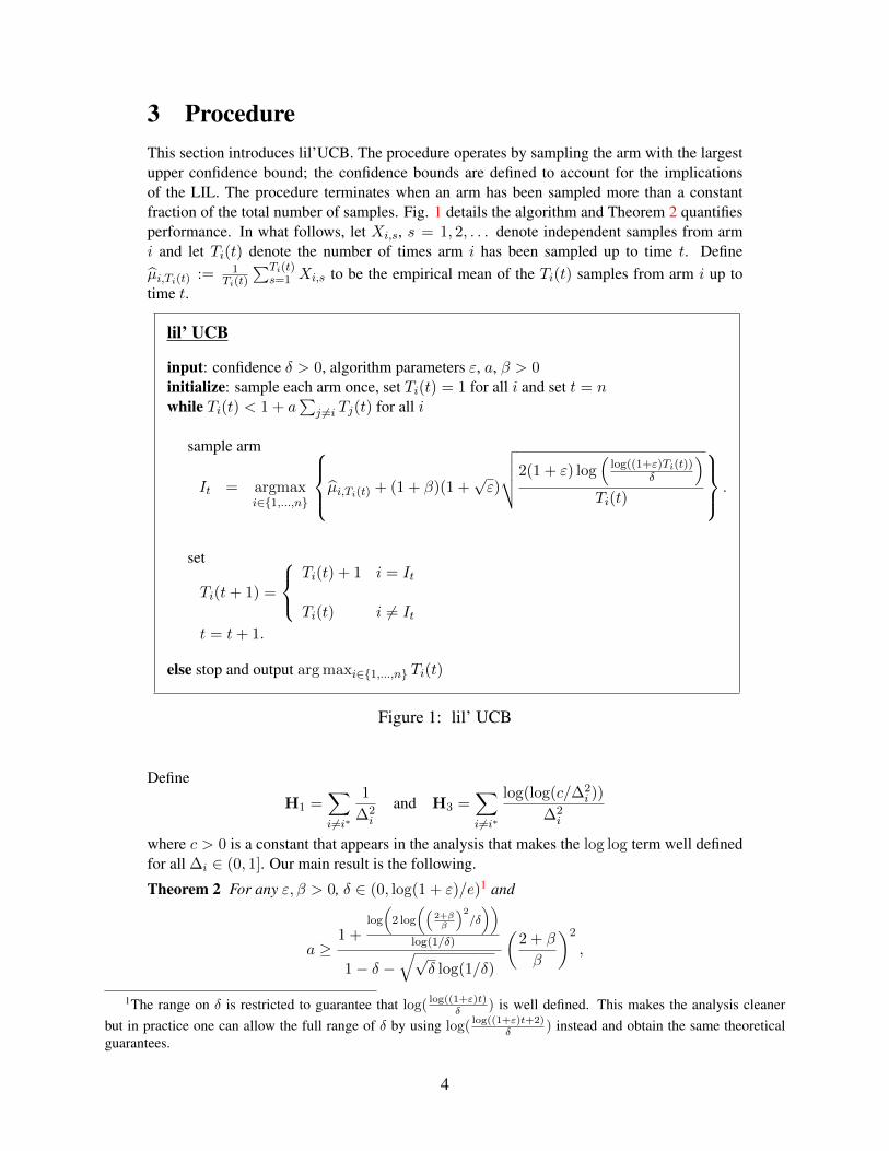
3 ProcedureThis section introduces lil’UCB. The procedure operates by sampling the arm with the largestupper confidence bound; the confidence bounds are defined to account for the implicationsof the LIL. The procedure terminates when an arm has been sampled more than a constantfraction of the total number of samples. Fig. 1 details the algorithm and Theorem 2 quantifiesperformance. In what follows, let Xi,s, s = 1, 2, . . . denote independent samples from armi and let Ti(t) denote the number of times arm i has been sampled up to time t. Defineµi,Ti(t) := 1

Ti(t)

∑Ti(t)s=1 Xi,s to be the empirical mean of the Ti(t) samples from arm i up to

time t.

lil’ UCB

input: confidence δ > 0, algorithm parameters ε, a, β > 0initialize: sample each arm once, set Ti(t) = 1 for all i and set t = nwhile Ti(t) < 1 + a

∑j 6=i Tj(t) for all i

sample arm

It = argmaxi∈1,...,n

µi,Ti(t) + (1 + β)(1 +√ε)

√√√√2(1 + ε) log(

log((1+ε)Ti(t))δ

)Ti(t)

.

set

Ti(t+ 1) =

Ti(t) + 1 i = It

Ti(t) i 6= Itt = t+ 1.

else stop and output arg maxi∈1,...,n Ti(t)

Figure 1: lil’ UCB

Define

H1 =∑i 6=i∗

1

∆2i

and H3 =∑i 6=i∗

log(log(c/∆2i ))

∆2i

where c > 0 is a constant that appears in the analysis that makes the log log term well definedfor all ∆i ∈ (0, 1]. Our main result is the following.

Theorem 2 For any ε, β > 0, δ ∈ (0, log(1 + ε)/e)1 and

a ≥1 +

log

(2 log

((2+ββ

)2/δ

))log(1/δ)

1− δ −√√

δ log(1/δ)

(2 + β

β

)2

,

1The range on δ is restricted to guarantee that log( log((1+ε)t)δ ) is well defined. This makes the analysis cleaner

but in practice one can allow the full range of δ by using log( log((1+ε)t+2)δ ) instead and obtain the same theoretical

guarantees.

4

with probability at least 1−√ρδ − 4ρδ

1−ρδ , lil’ UCB stops after at most c1H1 log(1/δ) + c3H3

samples and outputs the optimal arm where ρ = 2+εε

(1

log(1+ε)

)1+εand c1, c3 > 0 are con-

stants that depend only on ε, β.

Note that regardless of the choice of ε, β the algorithm obtains the optimal query complex-ity of H1 log(1/δ) + H3 up to constant factors. However, in practice some settings of ε, βperform better than others. We observe from the bounds in the proof that the optimal choice

for the exploration constant is β ≈ 1.66 but we suggest using β = 1 and a =(β+2β

)2. The

optimal value for ε is less evident as it depends on δ but we suggest using ε = 0.01. If one iswilling to forego theoretical guarantees, we recommend taking a more aggressive setting withε = 0, β = 0.5, and a = 1 + 10/n which is motivated by simulation results presented later.We prove the theorem via two lemmas, one for the total number of samples and one for thecorrectness of the algorithm. In the lemmas we give precise constants.

4 Proof of Theorem 2Before stating the two main lemmas that imply the result, we first present a finite form of thelaw of iterated logarithm. This finite LIL bound is necessary for our analysis and may alsoprove useful for other applications.

Lemma 1 Let X1, X2, . . . be i.i.d. centered sub-Gaussian2 random variables with scale pa-rameter σ. For any ε ∈ (0, 1) and δ ∈ (0, log(1 + ε)/e)3 one has with probability at least

1− 2+εε

(δ

log(1+ε)

)1+εfor any t ≥ 1,

t∑s=1

Xs ≤ (1 +√ε)

√2σ2(1 + ε)t log

(log((1 + ε)t)

δ

).

Proof We denote St =∑t

s=1Xs, and ψ(x) =

√2σ2x log

(log(x)δ

). We also define by induc-

tion the sequence of integers (uk) as follows: u0 = 1, uk+1 = d(1 + ε)uke.

Step 1: Control of Suk , k ≥ 1. The following inequalities hold true thanks to an unionbound together with Chernoff’s bound, the fact that uk ≥ (1 + ε)k, and a simple sum-integralcomparison:

P(∃k ≥ 1 : Suk ≥

√1 + ε ψ(uk)

)≤

∞∑k=1

exp

(−(1 + ε) log

(log(uk)

δ

))

≤∞∑k=1

(δ

k log(1 + ε)

)1+ε

≤(

1 +1

ε

)(δ

log(1 + ε)

)1+ε

.

2A random variable X is said to be sub-Gaussian with scale parameter σ if for all t ∈ R we have E[exptX] ≤expσ2t2/2.

3See footnote 1

5

Step 2: Control of St, t ∈ (uk, uk+1). Recall that Hoeffding’s maximal inequality4 states thatfor any m ≥ 1 and x > 0 one has

P(∃ t ∈ [m] s.t. St ≥ x) ≤ exp

(− x2

2σ2m

).

This implies that the following inequalities hold true (by using trivial manipulations on thesequence (uk)):

P(∃ t ∈ uk + 1, . . . , uk+1 − 1 : St − Suk ≥

√ε ψ(uk+1)

)= P

(∃ t ∈ [uk+1 − uk − 1] : St ≥

√ε ψ(uk+1)

)≤ exp

(−ε uk+1

uk+1 − uk − 1log

(log(uk+1)

δ

))≤ exp

(−(1 + ε) log

(log(uk+1)

δ

))≤(

δ

(k + 1) log(1 + ε)

)1+ε

.

Step 3: By putting together the results of Step 1 and Step 2 we obtain that with probability at

least 1− 2+εε

(δ

log(1+ε)

)1+ε, one has for any k ≥ 0 and any t ∈ uk + 1, . . . , uk+1,

St = St − Suk + Suk≤√ε ψ(uk+1) +

√1 + ε ψ(uk)

≤√ε ψ((1 + ε)t) +

√1 + ε ψ(t)

≤ (1 +√ε) ψ((1 + ε)t),

which concludes the proof.

Without loss of generality we assume that µ1 > µ2 ≥ . . . ≥ µn. To shorten notation wedenote

U(t, ω) = (1 +√ε)

√2(1 + ε)

tlog

(log((1 + ε)t)

ω

).

The following events will be useful in the analysis:

Ei(ω) = ∀t ≥ 1, |µi,t − µi| ≤ U(t, ω)

where µi,t = 1t

∑tj=1 xi,j . Note that Lemma 1 shows P(Ei(ω)) = O(ω). The following trivial

inequalities will also be useful (the second one is derived from the first inequality and the fact

4It is an easy exercise to verify that Azuma-Hoeffding holds for martingale differences with sub-Gaussian incre-ments, which implies Hoeffding’s maximal inequality for sub-Gaussian distributions.

6

that x+ax+b ≤

ab for a ≥ b, x ≥ 0). For t ≥ 1,

1

tlog

(log((1 + ε)t)

ω

)≥ c⇒ t ≤ 1

clog

(2 log((1 + ε)/(cω))

ω

), (1)

1

tlog

(log((1 + ε)t)

ω

)≥ c

slog

(log((1 + ε)s)

δ

)and ω ≤ δ ⇒ t ≤ s

c

log(2 log

(1cω

)/ω)

log(1/δ).

(2)

Lemma 2 Let γ = 2(2 + β)2(1 +√ε)2(1 + ε) and ρ = 2+ε

ε

(1

log(1+ε)

)1+ε. With probability

at least 1− 2ρδ one has for any t ≥ 1,

n∑i=2

Ti(t) ≤ n+ γ8eH1 log(1/δ) +n∑i=2

γlog(2 log(γ(1 + ε)/∆2

i ))

∆2i

.

Proof We decompose the proof in two steps.

Step 1. Let i > 1. Assuming that E1(δ) and Ei(ω) hold true and that It = i one has

µi+U(Ti(t), ω)+(1+β)U(Ti(t), δ) ≥ µi,Ti(t)+(1+β)U(Ti(t), δ) ≥ µ1,T1(t)+(1+β)U(T1(t), δ) ≥ µ1,

which implies (2+β)U(Ti(t),min(ω, δ)) ≥ ∆i. Thus using (1) with c =∆2i

2(2+β)2(1+√ε)2(1+ε)

one obtains that if E1(δ) and Ei(ω) hold true and It = i then

Ti(t) ≤2(2 + β)2(1 +

√ε)2(1 + ε)

∆2i

log

(2 log(2(2 + β)2(1 +

√ε)2(1 + ε)2/∆2

i /min(ω, δ))

min(ω, δ)

)≤ τi +

γ

∆2i

log

(log(e/ω)

ω

)≤ τi +

2γ

∆2i

log

(1

ω

),

where γ = 2(2 + β)2(1 +√ε)2(1 + ε), and τi = γ

∆2i

log(

2 log(γ(1+ε)/∆2i )

δ

).

Since Ti(t) only increases when It is played the above argument shows that the followinginequality is true for any time t ≥ 1:

Ti(t)1E1(δ) ∩ Ei(ω) ≤ 1 + τi +2γ

∆2i

log

(1

ω

). (3)

Step 2. We define the following random variable:

Ωi = maxω ≥ 0 : Ei(ω) holds true.

Note that Ωi is well-defined and by Lemma 1 it holds that P(Ωi < ω) ≤ ρω where ρ =

2+εε

(1

log(1+ε)

)1+ε. Furthermore one can rewrite (3) as

Ti(t)1E1(δ) ≤ 1 + τi +2γ

∆2i

log

(1

Ωi

). (4)

7

We use this equation as follows:

P

(n∑i=2

Ti(t) > x+

n∑i=2

(τi + 1)

)≤ ρδ + P

(n∑i=2

Ti(t) > x+

n∑i=2

(τi + 1)∣∣E1(δ)

)

≤ ρδ + P

(n∑i=2

2γ

∆2i

log

(1

Ωi

)> x

). (5)

Let Zi = 2γ∆2i

log(ρ

Ωi

), i ∈ [n]. Observe that these are independent random variables and since

P(Ωi < ω) ≤ ρω it holds that P(Zi > x) ≤ exp(−x/ai) with ai = 2γ/∆2i . Using standard

techniques to bound the sum of sub-exponential random variables one directly obtains that

P

(n∑i=2

Zi ≥ x

)≤ exp

(−min

x2

8e2‖a‖22,

x

4e‖a‖∞

)≤ exp

(−min

x2

8e2‖a‖21,

x

4e‖a‖1

).

(6)Putting together (5) and (6) with x = 4e‖a‖1 log(1/(ρδ)) one obtains

P

(n∑i=2

Ti(t) >

n∑i=2

(8eγ log(1/δ)

∆2i

+ τi + 1

))≤ 2ρδ,

which concludes the proof.

Lemma 3 Let ρ = 2+εε

(1

log(1+ε)

)1+ε. If

a ≥1 +

log

(2 log

((2+ββ

)2/δ

))log(1/δ)

1− δ −√√

δ log(1/δ)

(2 + β

β

)2

,

then for all i = 2, . . . n and t = 1, 2, . . . ,

Ti(t) < 1 + a∑j 6=i

Tj(t)

with probability at least 1−√ρδ − 2ρδ

1−ρδ .

Proof We decompose the proof in two steps.

Step 1. Let i > j. Assuming that Ei(ω) and Ej(δ) hold true and that It = i one has

µi + U(Ti(t), ω) + (1 + β)U(Ti(t), δ) ≥ µi,Ti(t) + (1 + β)U(Ti(t), δ)

≥ µj,Tj(t) + (1 + β)U(Tj(t), δ)

≥ µj + βU(Tj(t), δ),

which implies (2 + β)U(Ti(t),min(ω, δ)) ≥ βU(Tj(t), δ). Thus using (2) with c =(

β2+β

)2

one obtains that if Ei(ω) and Ej(δ) hold true and It = i then

Ti(t) ≤(

2 + β

β

)2 log

(2 log

((2+ββ

)2/min(ω, δ)

)/min(ω, δ)

)log(1/δ)

Tj(t).

8

Similarly to Step 1 in the proof of Lemma 2 we use the fact that Ti(t) only increases whenIt is played and the above argument to obtain the following inequality for any time t ≥ 1:

(Ti(t)−1)1Ei(ω)∩Ej(δ) ≤(

2 + β

β

)2

(2 log

((2+ββ

)2/min(ω, δ)

)/min(ω, δ)

)log(1/δ)

Tj(t).

(7)

Step 2. Using (7) with ω = δi−1 we see that

1Ei(δi−1) 1

i− 1

i−1∑j=1

1Ej(δ) > 1− α ⇒ (1− α)(Ti(t)− 1) ≤ κ∑j 6=i

Tj(t)

where κ =(

2+ββ

)2

1 +log

(2 log

((2+ββ

)2/δ

))log(1/δ)

. This implies the following, using that

P(Ei(ω)) ≥ 1− ρω,

P

∃ (i, t) ∈ 2, . . . , n × 1, . . . : (1− α)(Ti(t)− 1) ≥ κ∑j 6=i

Tj(t)

≤ P

∃ i ∈ 2, . . . , n : 1Ei(δi−1) 1

i− 1

i−1∑j=1

1Ej(δ) ≤ 1− α

≤

n∑i=2

P(Ei(δi−1) does not hold) +

n∑i=2

P

1

i− 1

i−1∑j=1

1Ej(δ) ≤ 1− ρδ − (α− ρδ)

.

Let δ′ = ρδ. Note that by a simple Hoeffding’s inequality and a union bound one has

P

1

i− 1

i−1∑j=1

1Ej(δ) ≤ 1− δ′ − (α− δ′)

≤ min((i− 1)δ′, exp(−2(i− 1)(α− δ′)2),

and thus we obtain with the above calculations

P

∃ (i, t) ∈ 2, . . . , n × 1, . . . :

(1− δ′ −

√√δ′ log(1/δ′)

)(Ti(t)− 1) ≥ κ

∑j 6=i

Tj(t)

≤

n∑i=2

(δ′i−1 + min((i− 1)δ′, exp(−2(i− 1)

√δ′ log(1/δ′)))

)≤√δ′ +

2δ′

1− δ′=√ρδ +

2ρδ

1− ρδ.

Treating ε and factors of log log(β) as constants, Lemma 2 says that the total numberof times the suboptimal arms are sampled does not exceed (β + 2)2 (c1H1 log(1/δ) + c3H3).

9

Lemma 3 states that only the optimal arm will meet the stopping condition with a = ca

(2+ββ

)2.

Combining these results, we observe that the total number of times all the arms are sampled

does not exceed (β+2)2 (c1H1 log(1/δ) + c3H3)

(1 + ca

(2+ββ

)2)

, completing the proof of

the theorem. We also observe using the approximation ca = 1, the optimal choice of β ≈ 1.66.

5 Implementation and SimulationsIn this section we investigate how the state of the art methods for solving the best arm problembehave in practice. Before describing each of the algorithms in the comparison, we brieflydescribe a LIL-based stopping criterion that can be applied to any of the algorithms.

LIL Stopping (LS) : For any algorithm and i ∈ [n], after the t-th time we have that thei-th arm has been sampled Ti(t) times and accumulated a mean µi,Ti(t). We can apply

Lemma 1 (with a union bound) so that with probability at least 1− 2+εε

(δ

log(1+ε)

)1+ε

∣∣µi,Ti(t) − µi∣∣ ≤ Bi,Ti(t) := (1 +√ε)

√√√√2σ2(1 + ε) log(

2n log((1+ε)Ti(t)+2)δ

)Ti(t)

for all t ≥ 1 and all i ∈ [n]. We may then conclude that if i := arg maxi∈[n] µi,Ti(t) andµi,Ti(t)

−Bi,Ti(t) ≥ µj,Tj(t) +Bj,Tj(t) then with high probability we have that i = i∗.

The LIL stopping condition is somewhat naive but often quite effective in practice for smallersize problems when log(n) is negligible. To implement the strategy for any fixed confidencealgorithm, simply run the algorithm with δ/2 in place of δ and assign the other δ/2 confidenceto the LIL stopping criterion. The algorithms compared were:

• Nonadaptive + LS : Draw a random permutation of [n] and sample the arms in an orderdefined by cycling through the permutation until the LIL stopping criterion is met.

• Exponential-Gap Elimination (+LS) [8] : This procedure proceeds in stages where ateach stage, median elimination [4] is used to find a ε-optimal arm whose mean is guar-anteed (with large probability) to be within a specified ε > 0 of the mean of the best arm,and then arms are discarded if their empirical mean is sufficiently below the empiricalmean of the ε-optimal arm. The algorithm terminates when there is only one arm thathas not yet been discarded (or when the LIL stopping criterion is met).

• Successive Elimination [4] : This procedure proceeds in the same spirit as Exponential-Gap Elimination except the landmark arm is equal to i := arg maxi∈[n] µi,Ti(t). Oneobserves that the algorithm’s usual stopping condition and the LIL stopping criterion areone in the same.

• lil’UCB (+LS) : The procedure of Figure 1 is run with ε = 0.01, β = 1, a = (2 +

β)2/β2 = 9, and δ =(

νε5(2+ε)

)1/(1+ε)for input confidence ν. The algorithm terminates

according to Fig. 1 or when the LIL stopping criterion is met.

• lil’UCB Heuristic : The procedure of Figure 1 is run with ε = 0, β = 1/2, a = 1 +10/n, and δ = ν/5 for input confidence ν. These parameter settings do not satisfy theconditions of Theorem 2, and thus there is no guarantee that this algorithm will find

10

the best arm. However, as the experiments show, this algorithm performs exceptionallywell in practice and therefore we recommend this lil’UCB algorithm in practice. Thealgorithm terminates according to Fig. 1.

• UCB1 + LS [11] : This is the classical UCB procedure that samples the arm

arg maxi∈[n]

µi,Ti(t) +√

2 log(t)Ti(t)

at each time t and terminates when the LIL stopping criterion is met.

We did not compare to PRISM of [7] because the algorithm and its empirical performance arevery similar to Exponential-Gap Elimination so its inclusion in the comparison would providevery little added value. We remark that the first three algorithms require O(1) amortizedcomputation per time step, the lil’UCB algorithms require O(log(n)) computation per timestep using smart data structures5, and UCB1 requires O(n) computation per time step. Dueto the poor computational scaling of UCB1 with respect to the problem size n, UCB1 was notrun on all problem sizes due to practical time constraints.

Three problem scenarios were considered over a variety problem sizes (number of arms).The “1-sparse” scenario sets µ1 = 1/4 and µi = 0 for all i = 2, . . . , n resulting in a hardnessof H1 = 4n. The “α = 0.3” and “α = 0.6” scenarios consider n + 1 arms with µ0 = 1 andµi = 1 − (i/n)α for all i = 1, . . . , n with respective hardnesses of H1 ≈ 3/2n and H1 ≈6n1.2. That is, the α = 0.3 case should be about as hard as the sparse case with increasingproblem size while the α = 0.6 is considerably more challenging and grows super linearlywith the problem size. See [7] for an in-depth study of the α parameterization. All experimentswere run with input confidence δ = 0.1. All realizations of the arms were Gaussian randomvariables with mean µi and variance 1/46.

Each algorithm terminates at some finite time with high probability so we first considerthe relative stopping times of each of the algorithms in Figure 2. Each algorithm was run oneach problem scenario and problem size 40 times. The first observation is that Exponential-Gap Elimination (+LS) appears to barely perform better than uniform sampling with the LILstopping criterion. This confirms our suspicion that the constants in median elimination arejust too large to make this algorithm practically relevant. It should not come as a great surprisethat successive elimination performs so well because even though it is suboptimal in the prob-lem parameters, its constants are small leading to a practical algorithm. The lil’UCB+LS andUCB1+LS algorithms seem to behave comparably and lead the pack of algorithms with the-oretical algorithms. The LIL stopping criterion seems to have a large impact on performanceof the regular lil’UCB algorithm, but it had no impact on the lil’UCB Heuristic variant (notplotted). While lil’UCB Heuristic has no theoretical guarantees of outputting the best arm, weremark that over the course of all of our tens of thousands of experiments, the algorithm neverfailed to terminate with the best arm.

In reality, one cannot always wait for an algorithm to run until it terminates on its ownso we now explore how the algorithms perform if the algorithm must output an arm at every

5To see this, note that the sufficient statistic for lil’UCB for deciding the next arm to sample depends only on µi,Ti(t)

and Ti(t) which only changes for an arm if that particular arm is pulled. Thus, it suffices to maintain an ordered list ofthe upper confidence bounds in which deleting, updating, and reinserting the arm requires justO(log(n)) computation.Contrast this with a UCB procedure in which the upper confidence bounds depend explicitly on t so that the sufficientstatistics for pulling the next arm changes for all arms after each pull, requiring Ω(n) computation per time step.

6The variance was chosen such that the analyses of algorithms that assumed realizations were in [0, 1] and usedHoeffding’s inequality were still valid using sub-Gaussian tail bounds with scale parameter 1/2.

11

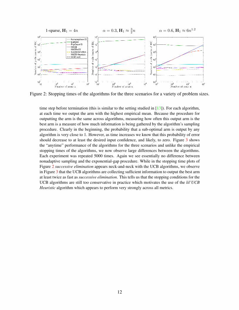
1-sparse, H1 = 4n α = 0.3, H1 ≈ 32n α = 0.6, H1 ≈ 6n1.2

Figure 2: Stopping times of the algorithms for the three scenarios for a variety of problem sizes.

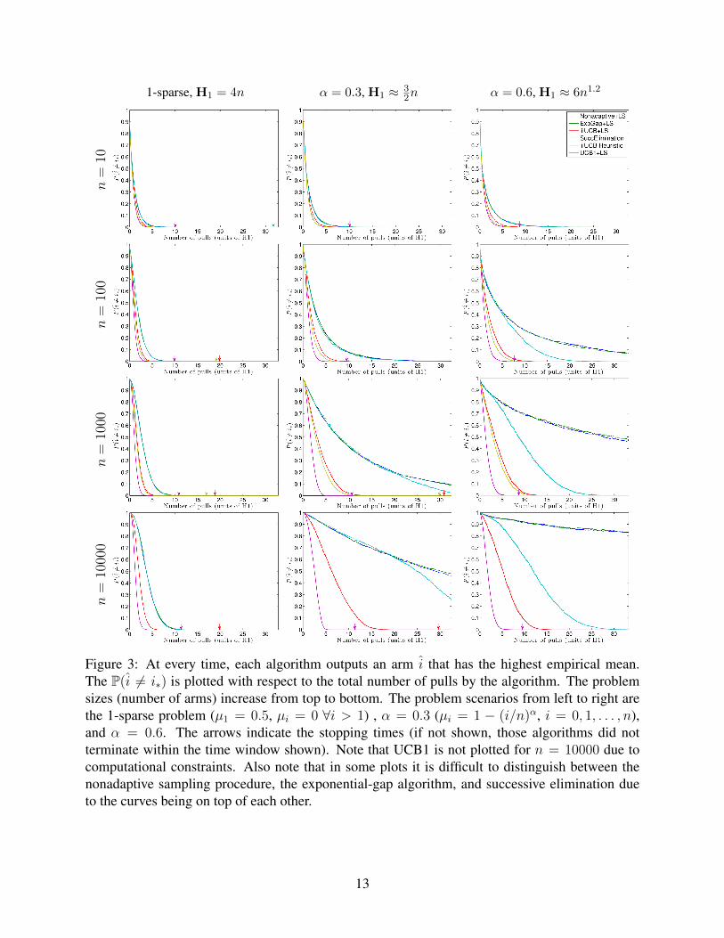
time step before termination (this is similar to the setting studied in [13]). For each algorithm,at each time we output the arm with the highest empirical mean. Because the procedure foroutputting the arm is the same across algorithms, measuring how often this output arm is thebest arm is a measure of how much information is being gathered by the algorithm’s samplingprocedure. Clearly in the beginning, the probability that a sub-optimal arm is output by anyalgorithm is very close to 1. However, as time increases we know that this probability of errorshould decrease to at least the desired input confidence, and likely, to zero. Figure 3 showsthe “anytime” performance of the algorithms for the three scenarios and unlike the empiricalstopping times of the algorithms, we now observe large differences between the algorithms.Each experiment was repeated 5000 times. Again we see essentially no difference betweennonadaptive sampling and the exponential-gap procedure. While in the stopping time plots ofFigure 2 successive elimination appears neck-and-neck with the UCB algorithms, we observein Figure 3 that the UCB algorithms are collecting sufficient information to output the best armat least twice as fast as successive elimination. This tells us that the stopping conditions for theUCB algorithms are still too conservative in practice which motivates the use of the lil’UCBHeuristic algorithm which appears to perform very strongly across all metrics.

12

n=

101-sparse, H1 = 4n α = 0.3, H1 ≈ 3

2n α = 0.6, H1 ≈ 6n1.2

n=

100

n=

1000

n=

10000

Figure 3: At every time, each algorithm outputs an arm i that has the highest empirical mean.The P(i 6= i∗) is plotted with respect to the total number of pulls by the algorithm. The problemsizes (number of arms) increase from top to bottom. The problem scenarios from left to right arethe 1-sparse problem (µ1 = 0.5, µi = 0 ∀i > 1) , α = 0.3 (µi = 1 − (i/n)α, i = 0, 1, . . . , n),and α = 0.6. The arrows indicate the stopping times (if not shown, those algorithms did notterminate within the time window shown). Note that UCB1 is not plotted for n = 10000 due tocomputational constraints. Also note that in some plots it is difficult to distinguish between thenonadaptive sampling procedure, the exponential-gap algorithm, and successive elimination dueto the curves being on top of each other.

13

References[1] Victor Gabillon, Mohammad Ghavamzadeh, Alessandro Lazaric, et al. Best arm identi-

fication: A unified approach to fixed budget and fixed confidence. 2012.

[2] Edward Paulson. A sequential procedure for selecting the population with the largestmean from k normal populations. The Annals of Mathematical Statistics, 35(1):174–180, 1964.

[3] Robert E Bechhofer. A sequential multiple-decision procedure for selecting the best oneof several normal populations with a common unknown variance, and its use with variousexperimental designs. Biometrics, 14(3):408–429, 1958.

[4] Eyal Even-Dar, Shie Mannor, and Yishay Mansour. Pac bounds for multi-armed banditand markov decision processes. In Computational Learning Theory, pages 255–270.Springer, 2002.

[5] Shie Mannor and John N Tsitsiklis. The sample complexity of exploration in the multi-armed bandit problem. The Journal of Machine Learning Research, 5:623–648, 2004.

[6] Shivaram Kalyanakrishnan, Ambuj Tewari, Peter Auer, and Peter Stone. Pac subset se-lection in stochastic multi-armed bandits. In Proceedings of the 29th International Con-ference on Machine Learning (ICML-12), pages 655–662, 2012.

[7] Kevin Jamieson, Matthew Malloy, Robert Nowak, and Sebastien Bubeck. On finding thelargest mean among many. arXiv preprint arXiv:1306.3917, 2013.

[8] Zohar Karnin, Tomer Koren, and Oren Somekh. Almost optimal exploration in multi-armed bandits. In Proceedings of the 30th International Conference on Machine Learn-ing, 2013.

[9] R. H. Farrell. Asymptotic behavior of expected sample size in certain one sided tests.The Annals of Mathematical Statistics, 35(1):pp. 36–72, 1964.

[10] DA Darling and Herbert Robbins. Iterated logarithm inequalities. In Herbert RobbinsSelected Papers, pages 254–258. Springer, 1985.

[11] Peter Auer, Nicolo Cesa-Bianchi, and Paul Fischer. Finite-time analysis of the multi-armed bandit problem. Machine learning, 47(2-3):235–256, 2002.

[12] Jean-Yves Audibert, Sebastien Bubeck, and Remi Munos. Best arm identification inmulti-armed bandits. COLT 2010-Proceedings, 2010.

[13] S. Bubeck, R. Munos, and G. Stoltz. Pure exploration in multi-armed bandits problems.In Proceedings of the 20th International Conference on Algorithmic Learning Theory(ALT), 2009.

14

A Condensed Proof of Lower BoundIn the following we show a weaker result than what is shown in [9]; nonetheless, it shows thelog log term is necessary.

Theorem 3 Let Xii.i.d.∼ N (∆, 1), where ∆ 6= 0 is unknown. Consider testing whether ∆ > 0

or ∆ < 0. Let Y ∈ −1, 1 be the decision of any such test based on T samples (possibly arandom number). If sup∆ 6=0 P(Y 6= sign(∆)) < 1/2, then

lim sup∆→0

E[T ]

∆−2 log log ∆−2> 0 .

We rely on two intuitive facts, each which justified more formally in [9].

Fact 1. The form of an optimal test is a generalized sequential probability ratio test (GSPRT),which continues sampling while

−Bt ≤t∑

j=1

Xi ≤ Bt

and stops otherwise, declaring ∆ > 0 if∑t

j=1Xj ≥ Bt, and ∆ < 0 if∑t

j=1Xj ≤ −Btwhere Bt > 0 is non-decreasing in t. This is made formal in [9].

Fact 2. If

limt→∞

Bt√2t log log t

≤ 1 (8)

then Y , the decision output by the GSPRT, satisfies sup∆ 6=0 P∆(Y 6= sign ∆) = 1/2.This follows from the LIL and a continuity argument (and note the limit exists as Btis non-decreasing). Intuitively, if the thresholds satisfy (8), a zero mean random walkwill eventually hit either the upper or lower threshold. The upper threshold is crossedfirst with probability one half, as is the lower. By arguing that the error probabilities arecontinuous functions of ∆, one concludes this assertion is true.

The argument proceeds as follows. If (8) is holds, then the error probability is 1/2. So wecan focus on threshold sequences satisfying limt→∞

Bt√2t log log t

≥ (1 + ε) for some ε > 0. Inother words, for all t > t1 some ε > 0, some sufficiently large t1

Bt ≥ (1 + ε)√

2t log log t.

Define the function

t0(∆) =ε2∆−2

2log log

(∆−2

2

)and let T be the stopping time:

T := inf

t ∈ N :

∣∣∣∣∣t∑i=1

Xi

∣∣∣∣∣ ≥ Bt.

15

Let S(∆)t =

∑tj=1Xj for Xj

iid∼ N (∆, 1). Without loss of generality, assume ∆ > 0. Ad-ditionally, suppose ∆ is sufficiently small, such that both t0(∆) > t1(ε) and ∆ ≤ ε (in thefollowing steps we consider the limit as ∆→ 0). We have

P∆(T ≥ t0(∆))

= P

t0(∆)−1⋂t=1

|S(∆)t | < Bt

= P

t1(ε)⋂t=1

|S(∆)t | < Bt ∩

t0(∆)−1⋂t=t1(ε)+1

S(0)t < Bt −∆t ∩ S(0)

t > −Bt −∆t

≥ P

t1(ε)⋂t=1

|S(∆)t | < Bt ∩

t0(∆)−1⋂t=t1(ε)+1

|S(0)t | < (1 + ε/2)

√2t log log t

(9)

= P

t1(ε)⋂t=1

|S(∆)t | < Bt

P

t0(∆)−1⋂t=t1(ε)+1

|S(0)t | ≤ (1 + ε/2)

√2t log log t

∣∣∣∣∣∣t1(ε)⋂t=1

|S(0)t | < Bt

≥ P

t1(ε)⋂t=1

|S(∆)t | < Bt

P

∞⋂t=t1(ε)+1

|S(0)t | < (1 + ε/2)

√2t log log t

(10)

where (9) holds when ε ≥ ∆ and (10) holds by removing the conditioning, and then byincreasing the number of terms in the intersection. To see that (9) holds, note that 2 log log t

t ≥(2∆ε

)2for all t ≤ t0(∆), which is easily verified when ε ≥ ∆ since

log log(ε2∆−2

2 log log(

∆−2

2

))log log

(∆−2

2

) ≥ 1.

Taking the limit as ∆→ 0, for any ε > 0, gives

lim∆→0

P∆(T ≥ t0(∆)) ≥ c(ε) > 0

which follows from (10), as the first term is non-zero for any ∆ (including ∆ = 0) sincet1(ε) <∞ and Bt > 0, and the second term is non-zero by the LIL for any ε > 0. Note that afinite bound on the second term can be obtained as in Section 2.

By Markov, E∆[T ]/t0(∆) ≥ P∆(T ≥ t0(∆)), and we conclude

lim∆→0

E∆[T ]

∆−2 log log ∆−2≥ ε2 c(ε) > 0

for any test with sup∆ 6=0 P(Y 6= sign(∆)) < 1/2.

16