Embed Size (px)
Citation preview

Lightweight Emulators for Multivariate
Deterministic Functions
Jonathan Rougier∗
Department of Mathematics
University of Bristol
February 8, 2007
Abstract
An emulator is a statistical model of a deterministic function, to be used
where the function itself is too expensive to evaluate within-the-loop of
an inferential calculation. Typically, emulators are deployed when deal-
ing with complex functions that have large and heterogeneous input and
output spaces: environmental models, for example. In this challenging
situation we should be sceptical about our statistical models, no matter
how sophisticated, and adopt approaches that prioritise interpretative
and diagnostic information, and the flexibility to respond. This paper
presents one such approach, candidly rejecting the standard Smooth
Gaussian Process approach in favour of a fully-Bayesian treatment of
multivariate regression which, by permitting sequential updating, al-
lows for very detailed predictive diagnostics. It is argued directly and
by illustration that the incoherence of such a treatment (which does not
impose continuity on the model outputs) is more than compensated for
by the wealth of available information, and the possibilities for general-
isation.
Draft copy: not to be circulated or cited without the author’s prior ap-
proval.
∗Department of Mathematics, University of Bristol, University Walk, Bristol BS8 1TW,U.K.; e-mail [email protected].
1

1 Introduction
An emulator is a stochastic representation of a deterministic function f , con-
structed using function evaluations; the term surrogate has also been used,
although recent practice has been to reserve this term for fast deterministic
approximations of f , e.g., from using a lower-resolution solver. Emulators are
useful wherever the function itself is costly to evaluate. A typical example is
a solver for a system described by a set of differential equations and equations
of state. The input vector x might simply be the initial value of the state
vector, but it might also include unknown system parameters. Even an eval-
uation time of just a few seconds would make this a costly function were it
necessary to explore a large input space. Thus emulators are useful in this
situation for optimisation calculations designed to choose ‘good’ values for x,
and also for inferential calculations designed to account for uncertainty in the
‘true’ x. Both of these activities fall under the general heading of computer
experiments ; see, e.g., Sacks et al. (1989), Koehler and Owen (1996) and Sant-
ner et al. (2003). Computer experiments for system inference, particularly
within a Bayesian framework, are discussed in Currin et al. (1991), Kennedy
and O’Hagan (2001), Craig et al. (1997, 2001), Goldstein and Rougier (2004,
2006a,b), Higdon et al. (2004), and Williams et al. (2006).
The challenge with building emulators is to find a parsimonious yet flexible
representation for our initial beliefs about f . This is hard when f is multi-
variate, particularly when the components of f(x) correspond to quantities
with quite different characteristics. For example, f might be a computer sim-
ulator for weather, where x denotes a particular value for the initial value of
the weather state-vector, and f(x) computes the evolution of that state-vector
in time. Thus f(x) comprises collections of space- and time-indexed values,
where each collection is a different type of quantity: pressure, temperature,
humidity, and so on. In the physics these values are all related in compli-
cated ways, and so our initial beliefs about f may be quite vague, possibly not
extending much beyond simple transformations of components of f(x) which
might be thought to make the resulting marginals more Gaussian.
It should go without saying that where the actions that follow from an anal-
ysis based on f will be costly or irreversible, then the emulator for f ought
to be carefully constructed. But not all computer experiments are so critical,
and even in those that are, an initial cheap emulator can still be informative
2

both in choosing the evaluation points, and in refining our knowledge about
f , in order that we might subsequently construct a more detailed and more
accurate emulator. Therefore there is certainly a case for a lightweight em-
ulator that runs out-of-the-box, which is easily tunable to quite vague prior
beliefs about f , and which is generalisable should the need arise. This pa-
per presents such an emulator. Section 2 describes its general principles; the
notation is given in Table 1. Section 3 considers an implementation for the
common situation where all inputs are continuous. Section 4 describes predic-
tive diagnostics. Section 5 compares the lightweight emulator proposed here
with its more heavy-weight alternative, the Smooth Gaussian Process. Sec-
tion 6 provides a simple illustration, including specifying an informative prior.
Section 7 describes and illustrates a tractable approach for generalising the
emulator, by mixing over priors. Section 8 concludes. An Appendix describes
the conjugate analysis used to construct the emulator, and the notation for
the various distributions.
2 The function and the emulator
2.1 The function
We write our vector-valued function as
fi(x) i ∈ I, x ∈ X
where X is a set of d-tuples and I is a discrete set with k components. We term
a value x an input, i an index variable, and fi(x) an output. An alternative
notation (e.g., as adopted by Kennedy and O’Hagan, 2001), is to write f(x; i),
particularly if i indexes a continuous set, such as spatial locations, or times.
In a predictive inference we typically have a well-specified index variables,
matching (a) the system observations we want to calibrate against, and (b) the
system quantities we wish to predict. In this case, there seems little need
to permit the set I to be continuous. In situations where we would like to
optimise over i, however (e.g., to find the best spatial location for a measuring
instrument), there may be advantages to the continuous formulation when it
is not possible to span the index-space with a high-resolution lattice, usually
because I is too large. Nevertheless, this is simply a notational matter, so
far as this paper is concerned. In our notation we drop the index variable
3

subscript to denote the full collection of outputs at any given input, and write
f(·) to refer to the function in full generality.
One fruitful source of functions such as f(·) is the Natural Sciences, where
models are constructed to represent complex systems, such as physical or envi-
ronmental systems, or biological systems. Perhaps the most popular approach
is the compartmental model, in which the behaviour of the state of the system
across a number of different compartments is described by ordinary differential
equations. One possible treatment (with a scalar state-vector, for simplicity)
is to take i to index the compartment, x to be the values of model parameters,
such as coefficients in the equations, and fi(x) to describe the equilibrium value
of the state quantity in compartment i with parameters x. Another treatment
is to specify a particular form of dynamic forcing, for example in the boundary
conditions, in which case i represents a tuple of compartment index and time
(or whatever the derivative is with respect to). In the more general setting
of a vector-valued state, or of partial differential equations, i may represent a
tuple of type, location and time. For example, in a climate model the value
fi(x) might denote sea-surface temperature in the Azores in the year 2050,
with model parameters x.
2.2 Emulating the function
These types of models can be extremely expensive to evaluate, and it is for
this reason that we need emulators. An emulator is synomymous with a dis-
tribution function
Πf (v, v′, . . . ; x, x′, . . . ) , Pr(f(x) ≤ v, f(x′) ≤ v′, . . .
)for any finite collection of xs and vs, where ‘,’ denotes ‘defined as’. Emulators
are distinguished from other types of functional interpolator, for example a
neural network, by providing a probabilistic assessment of uncertainty about
f(·). In inferences based on the function, the emulator allows us to account
for the uncertainty that arises from having only a limited number of function
evaluations, what O’Hagan and Oakley (2004) term code uncertainty. For
experimental design, emulators allow us to select a set of evaluations that is
expected to be highly informative about function behaviour over a range of
input values, both starting from scratch, and when augmenting an existing
design.
4

It is usually convenient to express an emulator implicity through the spec-
ification of more primitive uncertain quantities. We adopt the general form
f(x)T ≡ g(x)TB + u(x)T (1)
where g(·) is a q-vector of known regressors, B is a q × k matrix of uncertain
regression coefficients, and u(·) is a k-vector random field, termed the residual.
In our Lightweight Emulator (LWE) we hope to capture most of the vari-
ation in f(·) in terms of the fixed-length coefficient matrix B, allowing a rel-
atively simple specification for u(·). We adopt a Bayesian approach, where
we impose both structural and distributional restrictions on B and u(·), for
tractability. Our LWE emulator can be seen as a fully Bayesian conjugate
treatment of multivariate regression, or of multivariate kriging. A brief expla-
nation is given here, with more details in the Appendix. The focus of the paper
is not on this treatment per se, but on how we can use it when constructing
emulators.
We start by introducing an additional uncertain quantity Σ, a k×k variance
matrix. The structural restriction is that Σ separates B, u(x) and u(x′) when
x 6= x′, and consequently we must treat u(·) as a ‘nugget’, i.e. a process for
which
u(x) ⊥⊥ u(x′) | Σ x 6= x′. (2)
This restriction allows us to do sequential updating of B, Σ using model
evaluations, because it implies that
f(x) ⊥⊥ f(x′) | B, Σ x 6= x′. (3)
This can be summarised in the graphical model
B
11
11
11
11
DD
DD
D
Σ
==zzzzzzzzz//
!!BBB
BBBB
B u(x) ___ ⊕ f(x)
u(x′) ___ ⊕ f(x′)
(4)
An evaluation of f(x) is an observation on a set of known linear combinations
of B and u(x). This observation updates the joint distribution B, Σ. This
5

updated distribution feeds into our prediction of f(x′), where x′ 6= x, through
the updated joint distribution B, u(x′). Restricting u(·) to be a nugget is
contentious, and is discussed in section 5.
To make the updating of B, Σ tractable we impose further parametric
restrictions, all of which are specified with respect to our choice of regressors,
g(·):
1. The prior conditional distribution for the residual is stationary and Gaus-
sian
u(x) | Σ ∼ Nk (0, Σ) (5)
for all x ∈ X ;
2. The prior conditional distribution of the regression coefficients is Matrix
Normal:
B | Σ ∼ MNq×k (M, Ω, Σ) (6)
where the matrices M (q × k) and Ω (q × q) are hyperparameters;
3. The prior marginal distribution of Σ is Inverse Wishart
Σ ∼ IWk (S, δ) (7)
where S (k × k) and δ (scalar) are hyperparameters.
Taking (6) and (7) together, we say that B, Σ has a Matrix Normal Inverse
Wishart (MNIW) distribution, from which it follows that our emulator for
f(x) has a multivariate Student-t distribution. Furthermore, this emulator is
conjugate in the sense that updating by evaluations of the model just modifies
the hyperparameters M, Ω, S, δ. Prior or updated, the emulator mean and
variance functions, expressed in terms of the hyperparameters, are
E(f(x)
)= MTg(x) (8a)
cov(f(x), f(x′)
)=
w(x, x′)
δ − 2S, (8b)
provided that δ > 1 and δ > 2, respectively, where
w(x, x′) , g(x)TΩg(x′) + δ(x− x′); (8c)
where in (8c) the function δ(·) is the Dirac delta function (not to be confused
6

with δ, the hyperparameter of the Invese Wishart, or, below, δij, the Kronecker
delta function). The notation in this paper is summarised in Table 1.
One notable feature of (8) is that the variance function separates into a
part attributable to x and a part attributable to i. This separability is a
cornerstone of tractable statistical modelling over products of different types
of spaces: the implications have to be fairly brutal, in the light of the huge
reduction in complexity that results. In this case we can see that the ratio
cov(fi(x), fi′(x
′))
cov(fi(x′′), fi′(x′′′)
) =w(x, x′)
w(x′′, x′′′)
is dependent only on the four model-input values, and not on i, i′, the pair
of outputs we are selecting. For example, if we fix i = i′, x = x′ and x′′ = x′′′
and find that the variance of salinity at input x is exactly twice that at x′′,
then we must conclude that the variance of temperature at x is also exactly
twice that at x′′. Note that this is a feature of the emulator predictions, but
it does not constrain the way in which the emulator updates. That is to say,
if we considered a second emulator in which we partitioned the outputs and
treated them as block independent, then the predictive distributions within
each block would be the same in both emulators. Partitioning the outputs in
this way is beneficial only if we also allow our choices for the regressors or for
the prior hyperparameters to vary by block.
A discussion of this emulator is deferred until section 5, where it is con-
trasted with the more standard approach. A simple way to generalise the
emulator and ‘defeat’ the separability is discussed and illustrated in section 7.
2.3 Assessing the hyperparameters
The prior is summarised in terms of initial choices for the hyperparameters
Ψ , M, Ω, S, δ. But since the updating is conjugate, the following consider-
ations may also be applied to the updated hyperparameters, to derive summary
descriptions of the emulator at any stage of the process. To distinguish the
different choices, the prior values of the hyperparameters are labelled Ψ0.
As described in the Appendix, there exist ‘default’ choices for Ψ0 that
result in the expected values of the updated B and Σ being the Maximum
7

Table 1: Notation used in the paper.
Symbol Size Definition
Function quantities
x p Vector of function inputs, index j
f(x) k Vector of function outputs, index i
F ; X n× (k + p) Ensemble of function evaluations
Emulator quantities
g(x) q Vector of regressors, index r
B q × k Matrix of regressor coefficients
u(x) k Vector of residuals
Σ k × k ‘Column’ variance matrix
Hyperparameters, Ψ
M q × k Mean of B
Ω q × q ‘Row’ variance matrix
S k × k Scale matrix for Σ
δ scalar Degrees of freedom for Σ
Ψ0 Collection Prior hyperparameters
Other
`v(·) Legendre polynomial of order v
δ(·) Dirac delta function
δij Kronecker delta function
8

Likelihood (ML) estimators in multivariate regression, namely
Ω−1 = 0q×q, S = 0k×k, δ = 2, (9)
for all M , so we might add M = 0q×k. Where there are a very large number of
evaluations of the model these default choices may be acceptable, even though
S = 0 is very unlikely to be a reasonable summary of well-informed judgements
about f(·). In general, however, we should consider how to make informative
choices based on our (expert’s) judgements about the model.
One possibility is to make judgements about the conditional behaviour of
f(x), and how it varies for different x. Reasonable choices for Ψ0 can then
be inferred from (8). However, this is a very large collection of assessments,
unless it is judged that our prior for f(·) has quite simple structure.
An alternative approach is to treat the input itself as an uncertain quantity.
In many applications where f(·) is a model of a complex system, it is natural
to think of a ‘best’ or ‘correct’ input x∗: that input for which f(x∗) is the
best representation of the underlying system (see, e.g., Rougier, 2007, for a
discussion of this approach in climate modelling). Tracing uncertainty about
x∗ through to uncertainty about f(x∗) is known as uncertainty analysis, an
application where emulators have proved very useful for expensive functions
(O’Hagan et al., 1999; Oakley and O’Hagan, 2002). Then judgements about
f(x∗) can be used to augment those about f(x); x ∈ X. Reasonable choices
for Ψ0 can be inferred in conjunction with a distribution Πx∗ .
An effective way of simplifying this process is to use regressors g(·) that
are orthonormal with respect to Πx∗ , i.e.,
〈gr, gr′〉 ,∫
gr(x) gr′(x) dΠx∗(x) = δrr′ (10)
where δrr′ is the Kronecker delta, and r will be used to index the regressors.
We can take g1(x) = 1. Partitioning M as
M =
(M1
M2:
)1× k
(q − 1)× k,
9

we have, for orthonormal regressors,
E(f(x∗)
)= M1
T (11a)
var(f(x∗)
)= M2:
TM2: +tr Ω + 1
δ − 2S, (11b)
where x∗ ∼ Πx∗ , which follows directly from (8). Note that orthonormal
regressors are unitless, so that the columns of M have the same units as the
model-outputs, and Ω is unitless. The prior for M1 should be set according
to our judgements about the aggregate means. We may choose to treat the
prior for Ω as a diagonal matrix, because we have no opportunity to discern
the impact of its off-diagonal structure in these summaries.
Another way of summarising the hyperparameters for an uncertain x∗ is
through an ‘R2’ value for each output. We can think of R2 as the squared
correlation between the predicted and actual values, or
R2i ,
cov(µi(x
∗), fi(x∗))2
var(µi(x∗)
)var(fi(x∗)
) (12)
for output i, where µ(x) is the mean function given in (8a). For orthonormal
regressors, this simplifies to
R2i =
m2i
m2i + ξ2
i
ξ2i ,
tr Ω + 1
δ − 2Sii, (13)
where m2i is defined as the ith term on the diagonal of M2:
TM2:. Obviously
if the prior for M2: is 0, then the prior R2 values will also be 0. We can
extract more information out of the R2 calculation by focusing on subsets of
the regressors, such as the first r according to some ordering; in this case
the ‘R2i ’ value is m2
ir/(m2i + ξ2
i ), where m2ir is the ith term on the diagonal of
M2:rTM2:r. If these regressors were monomial terms, for example (section 3), it
might be interesting to compute the R2 values for the linear terms, and think
of all higher-order terms as being relegated to a generalised (non-stationary)
residual.
For Ψ0, we might hope to be able to assess reasonable values for M and for
the lumped parameters ξi, i = 1, . . . , k, by considering the unconditional mean
and variance, and possibly the R2 values (if we choose M2: 6= 0). To decompose
ξi into values for the hyperparameters diag Ω, δ and S, we might start with the
10

cautious choice δ = 3, which would represent minimal prior information with
a finite second moment. More generally, δ reflects our confidence in our prior
assessment in terms of the number of function evaluations that it might be
considered equivalent to. The value tr Ω/(tr Ω + 1) represents the proportion
of the expected conditional variance that is attributable to uncertainty in the
coefficients. If this can be fixed, and δ is chosen, then the diagonal of S
can be determined to give appropriate values for Sd(fi(x∗)). The off-diagonal
components of S can be parameterised through a correlation matrix capturing
simple structure in the model outputs, such as block independence, or spatio-
temporal effects.
All this might seem rather hit-or-miss, both in terms of our ability to
provide detailed quantification of our prior judgements about the model, and
in terms of how the particular choices for the hyperparameters can be settled
on. But this really misses the point: the real issue is the extent to which we do
better than the default ML choices for the hyperparameters, as given in (9),
if we are willing to make more detailed judgements. At the very least we can
take the ML choices as bounds, and investigate whether we feel comfortable
moving away from the bounds. We also have the possibility of generalising our
choice for Ψ0, if we judge that to be appropriate (section 7).
3 Continuous inputs
When all of the inputs are continuous, we can make some further suggestions
about the choice of regressors. A generalisation of the probability integral
tranform can be used to map the domain of f(·) onto the unit cube, on which
the transformed Πx∗ is independent and uniform (Rosenblatt, 1952). Often,
this extra mapping will not to be required, as it is a common judgement to
treat the components of x∗ as independent, bounded and uniform (possibly
after marginal transformations). But note also that in some applications we
will discover, during the experiment, that the model does not evaluate for
certain choices of inputs. Even if we are prepared to attach zero probability
to these ‘unsuccessful’ input values, we are still left with the problem that the
region of successful choices is not well-defined, nor is it easy to summarise.
This situation is not treatable using the methods of this section.
We will restrict attention to the case where Πx∗ is absolutely continu-
ous, and treat the domain of f(·) as [0, 1]d. The main thing this rules out
11

is ‘switches’ in x, which sometimes occur in physical models where we can
selectively activate subprocesses (see, e.g., the climate model in Murphy et al.,
2004). In this case we must think of f(·) as conditional on a given setting of
the various switches. If we so choose, we can build the bigger emulator which
includes both the continuous and discrete inputs, in which case the follow-
ing analysis holds for the continuous inputs only, expressed as a function of
the discrete ones. Regression-type approaches are natural for these types of
emulators: see, for example, Rougier et al. (2006).
3.1 Choice of regressors
Where f(·) is continuous and bounded on [0, 1]d we can use a tensor product
of Legendre polynomials for g(·), shifted from their usual domain of [−1, 1]
to [0, 1]. Each component gr(·) is a monomial that can be identified by the
exponent of each of the d input components, so that, if d = 2, (0, 0) would be
the constant, (1, 0) would be a linear term in x1, (0, 2) would be a quadratic
term in x2, (1, 1) would be a bilinear interaction term between x1 and x2, and
so on. If r is now generalised to be a d-vector of exponents, r ∈ Zd, then an
individual monomial can be represented as
gr(x) =d∏
j=1
`rj(xj)
where `v(·) is the Legendre polynomial of order v, shifted onto [0, 1], and j will
be used to index the model-inputs.
This structure generalises immediately to any situation where we construct
the regressors as tensor products, in such a way that we can index the individ-
ual terms: the rj do not have to be exponents. One very flexible approach is to
augment a small collection of global regressors for each input (e.g., a constant
and a linear term) with additional regressors from a given covariance function,
which gives rise to a set of approximately orthonormal prinicpal kriging func-
tions (see, e.g. Sahu and Mardia, 2005). These will be explored elsewhere; this
paper focusses on monomials.
An and Owen (2001) provide a convenient way of specifying collections of
12

monomials in terms of a triplet κ = (κ1, κ2, κ3). The constraints
d∑j=1
rj ≤ κ1
d∑j=1
(1− δ0rj) ≤ κ2 max
j∈1,...,drj ≤ κ3 (14)
define a collection of monomials. In words, κ1 is the maximum sum of the
exponents, κ2 is the maximum number of non-zero exponents, and κ3 is the
maximum single exponent. Thus κ = (2, 2, 2) would define a collection of
constant, linear, quadratic and bilinear interaction monomials: 21 altogether
if d = 5. It is straightforward to generate the complete set of monomials for
any given κ, using recursion. Using this approach, we can easily specify a large
collection of monomials for g(·), which we can hand-edit if we require more
control.
3.2 Specifying the prior for Ω
We can also use this monomial structure to simplify the task of specifying
ω , diag Ω in the prior (section 2.3). It is natural to follow the structure
in the monomial terms, and to take advantage of the orthonormality of the
regressors to relate coefficient uncertainty directly to output uncertainty. One
possibility is to use the parameterisation
ωr = τ0
d∏j=1
(τj)rj τ , (τ0, τ1, . . . , τd) 0, (15)
where we choose tau. The multiplier τ0 allows for scale differences between the
variances of BTg(x) and u(x), because the d-fold product in (15) is normalised
in the sense that its value for the intercept (r = 0) is always one.
There are other ways we might have specified ωr, for example in terms of
the values of the κ(r)-triple inferred from (14). The attraction of (15) is that
it allows us to duplicate values for τj across similar model-inputs. It often
happens in models of physical processes that a subset of the model-inputs
corresponds to the same type of quantity. In fact when d is large, it is usually
because x contains collections of quantities of the same type, often sub-indexed
by location and/or time. A model of a hydrocarbon reservoir, for example,
will have spatial fields of porosity and permeability as model-inputs (see, e.g.,
Craig et al., 1997). In this case we may choose to use a common value for τj
13

across all xj of the same type, leading to a large reduction in the number of
hyperparameters required in τ .
3.3 Emulator summaries
We can take advantage of the product structure of each gr(·) and the or-
thonormality of the legendre polynomials to derive simple expressions for low-
dimensional summaries of f(x∗), expressed in terms of main effects, two-way
interactions, and so on; Oakley and O’Hagan (2004) adopt a similar type of
approach in their treatment of sensitivity analysis. Consider conditioning on
some of the components of x∗, say those in the subset J ⊆ 1, . . . , d; for the
fully-aggregated case we would have J = ∅, while for the main effect with
respect to x∗j =xj we would have J = j. To reduce clutter we write (· | xJ)
for (· | x∗J =xJ) in what follows.
For the conditional expectation we have, starting from (8a),
E(f(x∗) | xJ) = E(E(f(x∗) | x∗) | xJ
)= MTh(xJ) (16a)
where
hr(xJ) , E(gr(x
∗) | xJ
)=∏j∈J
`rj(xj)×
∏j /∈J
δ0rj. (16b)
In words, the component hr(xJ) will be zero unless all of the not-conditioned-
on inputs are represented as constants, in which case it will be∏
J `rj(xj). In
the limits J = ∅ and J = 1, . . . , d we recover (11a) and (8a), respectively,
where we adopt the standard convention that products over the empty set
evaluate to 1.
For the conditional variance of the emulator expected value we have
var(E(f(x∗) | x∗) | xJ
)= MTvar
(g(x∗) | xJ
)M (17a)
where the variance may be computed from (16b) and the q× q matrix H(xJ),
where
Hrr′(xJ) , E(gr(x
∗) gr′(x∗) | xJ
)=∏j∈J
`rj(xj) `r′j
(xj)×∏j /∈J
δrjr′j. (17b)
Where J = ∅ we will have H(xJ) = Iq, the q × q identity matrix. For the
14

conditional expectation of the emulator variance we have
E(var(f(x∗) | x∗) | xJ
)=
tr H(xJ)Ω + 1
δ − 2S (18)
using (8b) and (17b). Adding (17a) and (18) gives the variance matrix var(f(x∗) | xJ
).
Again, in the limits J = ∅ and J = 1, . . . , d we recover (11b) and (8b). The
product structure in each gr(·) is useful in simplifying the expressions that
come between these two limiting cases. It is informative to contrast the two
sources of variance, since in some outputs the total variance may be dominated
by a sensitive mean function, while in others it may be dominated by a large
variance function.
4 Diagnostics
This paper advocates a fully-Bayesian approach with proper priors informed by
judgements about f(·). Even so, there are two compelling reasons for produc-
ing detailed diagnostic information. First, diagnostics are vital in selling the
emulator to the expert who constructed f(·), who may be suspicious about
a statistical framework that appears to replace the model he spent several
months constructing (this is a misconception, but a common and stubborn
one). Second, in the interests of tractability, our judgements about f(·) have
been structurally constrained and then shoe-horned into a MNIW prior. The
adoption of a prior we do not necessarily subscribe to compromises our quan-
tification of Ψ0, and we would want to perform a detailed sensitivity analysis
regarding our choices, and, possibly, generalise those choices somewhat.
The tractability of the LWE cuts both ways. It constrains our judgmements
about f(·), but it also ensures that an emulator is very simple to construct
for any given ensemble of evaluations. This means that we can use predictive
diagnostics to validate our prior judgements, and the structural and parametric
restrictions we have imposed. Predictive diagnostics are expensive, but very
valuable in situations where we expect our prior judgements to be influential
in the posterior. For example, in the illustration in section 6 we have 30
evaluations, but would like to use many more regressors in order to capture the
non-linearity and interactions we anticipate from our function. Consequently
the ensemble of evaluations will constrain certain linear combinations of the
regression coefficients, but will leave other combinations at their prior settings:
15

exactly what is constrained and what is not will depend in a subtle way on the
experimental design (see, e.g., Pistone et al., 2000). A predictive diagnostic
such as leave-one-out is informative about the model-specification, but also
gives us a clear visual picture of the predictive uncertainty that arises in the
updated emulator, n− 1 being close to n.
One limitation of leave-one-out, and its generalisations, is that it is hard to
construct simple summary measures across the whole ensemble. A diagnostic
which does provide such a summary uses the prequential approach (Dawid,
1984; Cowell et al., 1999). This is closely related to one-step-ahead, and so it
has the weakness that we cannot visualise our updated emulator’s predictive
uncertainty over a range of x values, since for much of the diagnostic we will be
updating with many less than n evaluations. So in practice, both diagnostics
are useful.
The prequential (‘predictive sequential’) approach is based on a sequential
analysis using increasing numbers of evaluations from the ensemble. Denote by
πm(·) the probability density function for predicting f(Xm) using evaluations
1, . . . ,m−1 from the ensemble. We can use this density to evaluate the actual
outcome Fm in terms of the logarithmic scoring rule
Sm , − ln πm(Fm) m = 1, . . . , n. (19)
Summing these scores gives
n∑m=1
Sm = − lnn∏
m=1
πm(Fm) = − ln π(F ; X, Ψ0) (20)
where π(F ; X, Ψ0) is the marginal density of the ensemble, showing that this
sum is invariant to the ordering of the evaluations in the ensemble. To compute
the full set of scores involves having a proper Ψ0 and then building n − 1
emulators of increasing size using the ensemble of evaluations. For an improper
Ψ0 e.g., the ML-prior given in (9), some of the evaluations would need to be
reserved.
We can calibrate any individual score in terms of its mean and variance
under the vaguely-specified null hypothesis
H0 : The statistical modelling choices are appropriate.
16

The predictive distribution of the emulator is a multivariate Student-t, denoted
Tk (v; µ, Σ, δ) in the standard parameterisation. Thus
Sm = −c +δ + k
2ln(1 + (k/δ) y
), (21a)
where c is the logarithm of the Student-t normalising constant and
y , k−1(v − µ)TΣ−1(v − µ). (21b)
Under the null hypothesis, y has a Fisher Fk,δ distribution; see, for example,
Bernardo and Smith (1994, p. 140, p. 123), although note there is a missing
k−1 in their definition of y.1 Therefore the mean and variance of Sm under
H0 can easily be computed using a one-dimensional numerical integration.
An alternative, when δ k so that ln(1 + (k/δ)y) ≈ (k/δ)y, is to use an
approximation based on the mean and variance of Fk,δ.
For sequential analysis, we can compute the mean and variance of∑i
m=1 Sm
in exactly the same way, although this would involve the inversion of an n×n
variance matrix. An alternative is to construct a prequential monitor,
Zi ,
∑im=1 Sm −
∑im=1 E(Sm)√∑i
m=1 var(Sm)i = 1, . . . , n. (22)
Under fairly broad conditions (Seillier-Moiseiwitsch and David, 1993), this
diagnostic has the property that as i → ∞ so the distribution of Zi tends to
the standard Gaussian under H0. This alternative has the advantage of being
‘free’, as it reuses quantities we have already computed; it also provides a more
precise calibration than standardised deviations from the mean, for large n.
1Proof: the k-vector v is a multivariate Student-t quantity with mean µ, scale matrix Σ,and degrees of freedom δ: it can be represented as
v − µ =(x− µ)√
w/δ
where the k-vector x is Gaussian with mean µ and variance Σ, w is χ2δ , and x and w are
independent. Hence
k−1(v − µ)T Σ−1(v − µ) =k−1(x− µ)T Σ−1(x− µ)
w/δ=
w′/k
w/δ
where w′ is χ2k and w′ and w are independent. This is the characterisation of the Fk,δ
distribution. Note that (3) in Mardia et al. (1979, p. 43) is incorrect.
17

Finally, a brief comment on the interpretation of diagnostic information,
particularly one-step-ahead and prequential. In the Bayesian approach it is
quite acceptable knowingly to hold prior judgements that are different from
those in the likelihood. In this situation the early values of the diagnostics will
be aberrant, while the likelihood is gradually asserting itself over the prior.
Crudely, we might expect this to take at least q evaluations, at which point ev-
ery linear combination of the regression coefficients has been updated. But dur-
ing this initialisation we are unable to distinguish between a prior/likelihood
conflict and a deeper problem arising from the our structural choices. One
solution is to contrast the diagnostics from our Ψ0 with those that arise when
we set Ψ0 equal to the tuned value
Ψ0 , argmaxΨ∈Γ
π(F ; X, Ψ) (23)
for some set Γ of our choosing. If this tuning does not improve the diagnostics
then we might reasonably conclude that there are inappropriate structural
restrictions in our emulator. An alternative tuning, which may be more robust,
is to maximise the ‘cross-validation density’ in place of the marginal density,
n∏i=1
π(Fi | F(i); X, Ψ) (24)
where F(i) denotes all but the ith evaluation (see, e.g., ?Gelfand and Dey,
1994). This can be computed directly from the leave-one-out diagnostic.
5 Comparison with standard methods
It is informative at this point to compare our treatment of the emulator with
the more standard approach using a Smooth Gaussian Process (SGP) prior
for f(·), as exemplified by, for example, Currin et al. (1991), Haylock and
O’Hagan (1996), and Kennedy and O’Hagan (2001). The first point to note is
that, as yet, the SGP has not been effectively generalised to multiple output
types, although it can handle mutiple indices (e.g., location) for a given type.
Therefore different output types have to be treated independently for any given
x. The LWE handles multiple types, within the constraints of the separable
covariance function (section 2.2).
Now focus on the case where f(x) is a scalar. In principle, the difference
18

between the LWE and the SGP is that the former represents the residual
as a nugget, while the latter uses a Gaussian process with continuous sample
paths (hence, ‘smooth’). The SGP requires the specification of a prior variance
function
κ(x, x′) , var(u(x), u(x′)
);
the LWE requires only the specification of a scalar prior variance. However,
it is important to distinguish between what may be done in principle, and
what is actually done in practice. With the SGP it appears to be difficult to
make an informed choice for the variance function κ(·, ·); the approach of Craig
et al. (1997, 2001) is an exception. Thus a parametric form is chosen, and then
the hyperparameters, typically controlling variance, roughness (differentiabil-
ity) and correlation length, are estimated from the ensemble, and plugged in.
Typically this choice of variance function follows well-trodden lines: the vari-
ance function is restricted to be stationary, and the correlation function to be a
product of (univariate) Matern correlation functions, and the hyperparameters
are estimated by maximising the marginal density or the cross-validation den-
sity (see, e.g., Santner et al., 2003). This separability across inputs is a very
strong structural restriction; it is discussed by O’Hagan (1998).
The estimation of the hyperparameters in the SGP emulator has important
implications for the choice of regressors. The residual has a representation in
terms the regressors, and so there is an identification problem between the
variance function hyperparameters and the regression coefficients. This prob-
lem has bedeviled the technique of universal kriging in Spatial Statistics (see,
e.g., Cressie, 1991, sec. 3.4). One solution, commonly adopted with the SGP,
is to limit the number of regressors, often to just a constant (possibly extended
to linear terms): this is akin to ordinary kriging in Spatial Statistics (Cressie,
op. cit.); a more sophisticated estimation method for the hyperparameters can
also help. Another is to keep the regressors but dispense with the structured
residual, as done by the LWE: this is trend surface prediction. Another is to
adopt a fully Bayesian hyperarchical approach, avoiding the problem of directly
quantifying the hyperparameters (see, e.g., Banerjee et al., 2004). However,
this typically involves Markov chain Monte Carlo (MCMC), and does not scale
well to applications with large numbers of inputs, or where large numbers of
emulators are to be constructed, for diagnostic purposes.
Now let’s examine the strengths and weaknesses of the nugget residual. The
19

weakness is easy to spot. The LWE will not, by default, perfectly interpolate
the ensemble. If f(·) is a smooth deterministic function then this is simply
wrong, because if f(x) is known then we ought to have
limx′→x
E([
f(x′)− f(x)]2)
= 0.
O’Hagan (2006) defines perfect interpolation as a key desideratum of emula-
tors. Now the case for the defence. First, if the residual variance is small then
this failure to interpolate perfectly will make little difference in practice, when
using the emulator to predict the behaviour of the function over a range of
possible input values. We can investigate the size of the residual and compare
it to var(f(x)
)for different x, and also to E
(var(x∗)
), so that we can satisfy
ourselves that it is small. Where it is not, we have the option of refining our
choice of regressors. Second, in many applications we will choose not to model
f(x) as a function of all of its inputs, but to focus on a subset. This has been
a common theme since the inception of the field of computer experiments (see,
e.g., Owen et al., 1989); Craig et al. (1996, 1997) refer to the components of
this subset as the active inputs. Treating f(·) as an explicit function only of
the active inputs, there will be unattributable variation from the non-active
inputs, which necessitates the inclusion of a nugget such as the LWE residual.
Now to the benefit of the nugget residual. The LWE is fast to fit, and its
computational cost scales linearly in n, in the sense that the emulator can be
updated sequentially, one evaluation at a time. The cost of the SGP, though,
scales as n3, this being the cost of the Choleski decomposition required to
invert an n×n variance matrix (see, e.g., Golub and Van Loan, 1989, p. 142).
With single-type multivariate output, this cost scales as (kn)3, unless an outer
product design has been used (scales as n3), which has its own drawbacks; see
Kennedy and O’Hagan (2001) and the discussion in Rougier (2001). As noted
by Koehler and Owen (1996, p. 265), the cost of even one inverse will rapidly
become prohibitive as the ensemble grows. The challenge of approximating this
calculation has been much studied in Spatial Statistics, using both subsets of
the ensemble (see, e.g., Besag, 1975; Jones and Vecchia, 1993) or sparse matrix
methods (Cornford et al., 2004). This is an extra layer of complexity that is
completely absent in the LWE. Another complication with the SGP when n
is large is that the variance matrix can be ill-conditioned, in which case one
solution is to inflate the diagonal (Higdon et al., 2004): of course this means
20

that that the emulator no longer interpolates perfectly.
So lack of speed is the drawback of the SGP. This should be measured not
in clock-time, though, but in the opportunity to perform detailed diagnostics.
There is no sense in which a SGP requires less diagnostic checking than a LWE:
in practice both approaches make strong structural choices, and both may be
expected to extrapolate badly even in some of the cases where they interpolate
well. On this basis, predictive diagnostics are vital for building confidence in
the emulator. These predictive diagostics require us to build many emulators.
The slowness of the SGP becomes much more acute, and corners may have
to be cut, e.g. by not re-estimating the variance function hyperparameters for
each different subset of the ensemble. Exactly the same comments apply in
situations where we would like to experiment with different transformations of
the model-inputs and model-outputs, and different choices of regressors.
To summarise, consider the following question: if you discovered that a
LWE did not perform well, would you then be happy to switch to a SGP? I
for one would be wary. The same applies the other way around, of course,
but the difference is that the LWE costs almost nothing to fit and can be
extensively audited, so is the natural candidate to try first.
6 Illustration
This illustration is based on the Atlantic Ocean compartmental model of Zick-
feld et al. (2004), and uses an ensemble constructed for Goldstein and Rougier
(2006b). This comprises n = 30 evaluations designed as a maximin latin hy-
percube over d = 5 continuous inputs, with k = 7 outputs. This small number
of evaluations highlights the role of the prior.
The calculations were performed in the R statistical programming environ-
ment (R Development Core Team, 2004).
6.1 Specifying the prior
Section 2.3 discusses how we might specify informative priors for the emulator.
Here I outline some simple choices based on my experiences of this model, and
of the system it is designed to represent. These choices are genuine attempt
to describe my judgements, although the values have been tweaked a little to
make the illustration more informative.
21

Regressors. The inputs are continuous, and I choose to use monomial re-
gressors up to cubics and three-way interactions. In the scheme of An and
Owen (2001), this is described by the triplet κ = (3, 3, 3); see section 3.1. This
gives q = 56 regressors in all. (I tried more regressors, including quartics, but
it appeared to make no difference.)
Coefficient means. The prior values for the first row of M are set according
to my judgements about the unconditional mean of f(x∗), where x∗ is uniform
on the range of possible values for x, which is [0, 1]5, after transforming the
inputs. The first three model-outputs are Atlantic Ocean temperatures in
Centigrade, for which I chose 10, 5, 15 (South, North, Tropical). The fourth
and fifth are salinity differences in Practical Salinity Units, for which I chose
0 and 0. The sixth is meridional overturning in Sverdrups (Sv, 106 m3 s−1), for
which I chose 20, and the seventh is critical freshwater forcing in Sv, for which
I chose 0.1. This final output is likely to have the most complex relationship
with the inputs, as it is the solution of an inverse problem.
I have strong prior judgements about the relationship between the first
three inputs and the first three outputs. Let v1:3 , (v1, v2, v3) be atmospheric
temperature forcing in the South, North and Tropical compartments. Then,
to first order, I judge that
∆f1:3 ∝ ∆v1:3. (25)
The inputs x1:3 are related to v1:3 by
x1:3 =
0 1 0
1 −1 0
−1 0 1
v1:3, or x1:3 ≡ A v1:3 ; (26)
this was to ensure that the ordering v2 ≤ v1 ≤ v3 was preserved in the choices
of x1:3 ∈ [0, 1]3. Therefore, in terms of model-inputs and model-outputs,
∆f1:3 ∝ ∆(A−1x1:3). (27)
I chose the proportionality constant to be 3, because the model-inputs are
rescaled, but the model-outputs are not. Thus the values 3A−1 are used in M
to relate the linear regressors in the first three model-inputs to the first three
model-outputs. All the other prior values of M are set to zero.
22

Variances. Appropriate values for the variance var(f(x∗)
)can now be in-
ferred from choices for the lumped parameters ξ2i , defined in (13). My choices
and the resulting implied values are
ξi: 3 3 3 0.2 0.2 5 0.1
Sd(fi(x
∗)): 5.2 4.2 6 0.2 0.2 5 0.1
R2i (%): 67 50 75 0 0 0 0
where the difference between the first three outputs (columns) and the others
four is due to non-zero values in M .
Finally, I must represent the value of ξ2i in terms of choices for diag Ω, δ,
and S, where I choose to treat the prior Ω as diagonal. I choose δ = 3. I expect
the residual variance to be quite small, so I choose tr Ω = 9, which implies that
Sii = ξ2i /10. I choose to zero the off-diagonal elements in S. For the actual
values of diag Ω, I use the approach in section 3.2, and choose τj = 0.1 for
j = 1, 2, 3, so that the standard deviation of a cubic coefficient is 0.1 that of a
linear coefficient: I expect the response to the three temperature inputs to be
mainly linear. I choose τj = 1 for j = 4, 5: I expect the response to these two
inputs to be more complicated. It follows that τ0 = 0.75, to satisfy tr Ω = 9.
Prior and posterior. Samples from this prior emulator are shown in Fig-
ure 1, showing how the 7 outputs respond to x2 (11 values across the range
[0, 1]), with the other inputs held at their central values. Each of these samples
(10 in all) has a (11 × 7)-dimensional Student-t distribution. Note that the
roughness in each sampled path in x2 is due to the treatment of the residual
as a nugget: this roughness would have been smaller had I chosen tr Ω larger,
which I might have done had I chosen to include more regressors.
The prior emulator is updated with the ensemble of 30 evaluations. Samples
from the updated emulator are given in Figure 2: this is comparable with
Figure 1. My prior judgements about the three temperatures seem to have
been well-founded.
23

0.0 0.2 0.4 0.6 0.8 1.0
510
15
T1
xpts
0.0 0.2 0.4 0.6 0.8 1.0
34
56
78
T2
xptst(
tmp)
0.0 0.2 0.4 0.6 0.8 1.0
1015
20
T3
xpts
0.0 0.2 0.4 0.6 0.8 1.0
−0.
4−
0.2
0.0
0.2
S2mS1
xpts
0.0 0.2 0.4 0.6 0.8 1.0
−0.
10.
10.
3
S3mS2
xpts
t(tm
p)
0.0 0.2 0.4 0.6 0.8 1.0
−5
515
25
meq
0.0 0.2 0.4 0.6 0.8 1.0
−0.
050.
050.
15
F1crit
t(tm
p)
Figure 1: 10 samples from the prior emulator, for f as a function of x2 withthe other inputs set at their central values.
24

0.0 0.2 0.4 0.6 0.8 1.0
510
15
T1
xpts
0.0 0.2 0.4 0.6 0.8 1.0
34
56
78
T2
xptst(
tmp)
0.0 0.2 0.4 0.6 0.8 1.0
1015
20
T3
xpts
0.0 0.2 0.4 0.6 0.8 1.0
−0.
4−
0.2
0.0
0.2
S2mS1
xpts
0.0 0.2 0.4 0.6 0.8 1.0
−0.
10.
10.
3
S3mS2
xpts
t(tm
p)
0.0 0.2 0.4 0.6 0.8 1.0
−5
515
25
meq
0.0 0.2 0.4 0.6 0.8 1.0
−0.
050.
050.
15
F1crit
t(tm
p)
Figure 2: 10 samples from the updated emulator, comparable to those inFigure 1.
25

6.2 Diagnostics
Section 4 discusses diagnostics for the emulator. Figure 3 shows the leave-one-
out prediction errors. This Figure also provides a clear picture of the impact of
the separability of the emulator variance function (section 2.2). Treating the
ensembles in each of the 30 cases as almost the same, the pattern of relative
uncertainty is nearly duplicated across the 7 panels. For example, the ratio of
the predictive uncertainty between evaluations 9 and 10 is always about 0.8,
no matter what output.
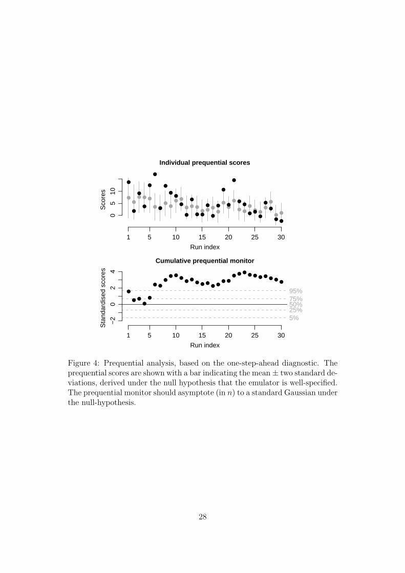
Figure 4 shows the prequential diagnostics, based on one-step-ahead: while
these are not terrible, neither are they very encouraging. To investigate the
effect of my prior choices, the prior hyperparameters were tuned to maximise
the marginal density of the evaluations. This tuning was not unconstrained:
the ξ2i quantities were permitted to vary by output type (four multipliers),
the τj were permitted to vary by input type (three multipliers), and the trace
of Ω was allowed to vary (one multiplier). The tuning process reduced the
summed prequential scores from 157.0 to 41.1. The effect on the prequential
diagnostics is shown in Figure 5; these are now acceptable (evaluation 21
has an extremely low value of x5). The aberrant prequential diagnostics in
Figure 4 would seem to have resulted from a disagreement between my prior
and my likelihood, rather than the structural constraints of the LWE. For the
remainder of this section, though, I continue with my original prior choices; in
practice a reconsideration of my prior in the light of the tuned values might
be advisable, possibly including some higher-order x5 regressors.
26

T1
Index
1 5 10 15 20 25 30
−5
05
1015
20
T2
Index
1 5 10 15 20 25 30
02
46
810
T3
Index
1 5 10 15 20 25 30
05
1015
2025
S2mS1
Index
1 5 10 15 20 25 30
−1.
0−
0.5
0.0
0.5
S3mS2
Index
1 5 10 15 20 25 30
−0.
40.
00.
40.
8
meq
1 5 10 15 20 25 30
−20
020
40
F1crit
1 5 10 15 20 25 30
−0.
10.
00.
10.
20.
3
Figure 3: Leave-one-out prediction errors. The horizontal axis shows the eval-uations. The grey bars and dots show the predicted 2.5th, 50th, and 97.5thpercentiles using all but the indexed evaluation; the black dots show the actualvalues.
27
Individual prequential scores
Run index
Sco
res
1 5 10 15 20 25 30
05
10
Cumulative prequential monitor
Run index
Sta
ndar
dise
d sc
ores
1 5 10 15 20 25 30
−2
02
4
5%25%50%75%95%
Figure 4: Prequential analysis, based on the one-step-ahead diagnostic. Theprequential scores are shown with a bar indicating the mean± two standard de-viations, derived under the null hypothesis that the emulator is well-specified.The prequential monitor should asymptote (in n) to a standard Gaussian underthe null-hypothesis.
28

Individual prequential scores
Run index
Sco
res
1 5 10 15 20 25 30
−10
010
20
Cumulative prequential monitor
Run index
Sta
ndar
dise
d sc
ores
1 5 10 15 20 25 30
−2
01
2
5%
25%50%75%
95%
Figure 5: Prequential analysis, after tuning the prior hyperparameters to max-imise the marginal density of the ensemble. See Figure 4 for details.
29

6.3 Summaries
Section 3.3 describes how we can summarise the emulator reponse to a subset
of the inputs in terms of the conditional mean and variance, integrating out
other inputs according to some distribution x∗ as though they were nuisance
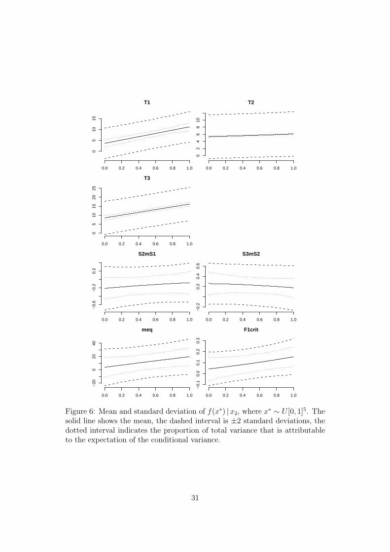
parameters. I choose x∗ to be uniform on [0, 1]5. Figure 6 shows the function
responses to x2, represented in this way. Note that the difference between
Figure 2 and Figure 6 is that in the former the other four inputs are set to 0.5,
while in the latter they are integrated out.
Figure 6 shows a clear difference between the three temperature outputs,
T1, T2, and T3, and the other outputs, e,g., F1crit, conditionally on x2. In the
temperatures almost all of the variance is attributable to the mean function.
In F1crit much of the variance is attributable to the variance function. We
can infer that the mean functions of the temperatures are highly sensitive to
the other four inputs, while the mean function of F1crit is not. In fact, we
know this to be the case, because the temperatures depend strongly on x1 and
x3 as well.
Figure 7 shows how x2 and x5 interact to determine one of the salinity
differences, output 5, with the other three inputs integrated out.
Section 2.3 also discussed numerical summaries, such as ‘R2’ values. These
are shown in the top panel of Figure 8, plotted against increasing sets of
regressors in the grevlex ordering. We can see that the three temperatures
are well-explained by linear regressors alone with no interactions; i.e. f1:3(x) is
effectively linear in x. The other outputs are poorly explained by linear terms
alone; including higher-order terms helps, but not much. The bottom panel
shows the absolute sizes of the coefficients, indicating the greater non-linearity
of the responses of the non-temperature outputs. Within each degree-block,
the ordering favours the non-temperature inputs; the preponderance of sizeable
coefficients in the region starting from regressor 22 indicates that these inputs
are the more important contributors to the non-linear responses.
30
0.0 0.2 0.4 0.6 0.8 1.0
05
1015
T1
xpts
0.0 0.2 0.4 0.6 0.8 1.0
02
46
810
T2
xpts
E
0.0 0.2 0.4 0.6 0.8 1.0
05
1015
2025
T3
xpts
0.0 0.2 0.4 0.6 0.8 1.0
−0.
6−
0.2
0.2
S2mS1
xpts
0.0 0.2 0.4 0.6 0.8 1.0
−0.
20.
20.
40.
6
S3mS2
xpts
E
0.0 0.2 0.4 0.6 0.8 1.0
−20
020
40
meq
0.0 0.2 0.4 0.6 0.8 1.0
−0.
10.
00.
10.
20.
3
F1crit
E
Figure 6: Mean and standard deviation of f(x∗) |x2, where x∗ ∼ U [0, 1]5. Thesolid line shows the mean, the dashed interval is ±2 standard deviations, thedotted interval indicates the proportion of total variance that is attributableto the expectation of the conditional variance.
31

0.0 0.2 0.4 0.6 0.8 1.0
0.0
0.2
0.4
0.6
0.8
1.0
Mean
x2
xptsx 5
0.0 0.2 0.4 0.6 0.8 1.0
0.0
0.2
0.4
0.6
0.8
1.0
Std dev.
x2
xpts
Figure 7: Mean and standard deviation of f5(x∗)|x2, x5, where x∗ ∼ U [0, 1]5.
R2 values for each output
1:q1 10 20 30 40 50
0.0
0.4
0.8
F1critS2mS1meqS3mS2
T1T3T2
Two Degree three
Absolute values of updated regression coefficients
Monomials in grevlex ordering1 10 20 30 40 50
T1T2T3
S2mS1S3mS2
meqF1crit
Two Degree three
Figure 8: (1) Top panel. ‘R2’ values for each of the outputs after updating,shown for increasing sets of monomials in grevlex ordering. (2) Bottom panel.Absolute values (darker signifies larger) of the updated expectations of theregression coefficients (excluding the intercept); same ordering. Each set ofcoefficients is rescaled to be unitless by dividing through by the range of eachoutput in the ensemble.
32

7 Mixing over the hyperparameters
We would like to break out from the structural restrictions of the LWE with its
MNIW structure to a more general emulator, but without sacrificing tractabil-
ity. We would also like to account for difficulties in quantifying the prior hyper-
parameters, Ψ0. The simplest way to achieve both of these goals is to mix over
m different choices of Ψ0, i.e. to generalise our prior to
B, Σ | ω= i ∼ MNIWk
(Ψ
(i)0
)Pr(ω= i) = λi i = 1, . . . ,m
(28)
where λ , (λ1, . . . , λm) is a hyperparameter of probabilities.
The crucial quantity for computing the posterior mixture distribution is
the marginal density of the ensemble, π(F ; X, Ψ0), which is computed ‘for
free’, along with the prequential diagnostics, see (20). After updating us-
ing the ensemble, the posterior emulator is a mixture of the emulators from
each of the prior choices for Ψ0, with the weights themselves updated to
λi π(F ; X, Ψ
(i)0
)and renormalised so that
∑mi=1 λi = 1. Thus with a mixture
prior, we have an extended conjugate analysis over the set of hyperparametersΨ(1), . . . , Ψ(m), λ
.
Berger and Berliner (1986) provide a different take on the same type of
calculation, in which the prior hyperparameters may be partly or completely
tuned using the ensemble. In the simplest case, this involves mixing over
two choices of hyperparameters: the elicited prior Ψ(1)0 = Ψ0, and a data-
determined prior Ψ(2) = Ψ0, given in (23). In the extreme choice of λ1 = 0,
λ2 = 1, and Γ unconstrained, this gives rise to the standard parametric em-
pirical Bayes approach (see, e.g., Carlin and Louis, 2000), where the hyper-
parameters for the prior are determined by maximising the marginal density
of the ensemble, and then plugged in. Berger and Berliner themselves suggest
using a small value for λ2, in order to ‘robustify’ the prior, although they are
understandably cautious about whether this genuinely promotes robustness.
33

The mean and variance with the mixture prior are
E(f(x)
)= MTg(x) (29a)
cov(f(x), f(x′)
)=
m∑i=1
λi
[M (i) − M
]Tg(x)g(x′)T
[M (i) − M
]+
m∑i=1
λiw(i)(x, x′)
δ(i) − 2S(i) (29b)
where
M ,m∑
i=1
λi M(i) (29c)
w(i)(x, x′) , g(x)TΩ(i)g(x′) + dirac(x− x′) (29d)
(cf. eq. (8)). By inspection of (29b) we can see that a separable variance
function is only preserved when mixing if M (i) = M and S(i) ∝ S, for all i, in
which case we have
cov(f(x), f(x′)
)=
[m∑
i=1
λi ciw(i)(x, x′)
δ(i) − 2
]S (30)
for some given scalars ci satisfying S(i) = ci S. Therefore a mixture prior gives
us an easy way to ‘defeat’ separability, if we so choose, and the degree to which
we defeat it will depend on the range of values we select for M (i), and the way
in which we allow the components of S(i) to vary independently of one another.
Note, though, that all of this comes to naught if after updating we find that
the λ values concentrate onto a single i; but at least in this case we have given
non-separability a chance to emerge, should it want to.
For inference and diagnostics, it is incovenient that the mixture prior does
not give rise to a readily-available predictive distribution (i.e., one that is al-
ready inplemented in standard statistical software). A simple alternative for
prediction is to use sampling. Each of the m emulators is built and updated
marginally, and then a draw is made from the predictive distribution after first
selecting one of the emulators according to the probabilities λ, also updated.
This allows us to compute leave-one-out and one-step-ahead diagnostics, with
appropriate credible intervals under H0. For the prequential diagnostics, the
statistic Sm can still be calculated easily, as can its mean and variance un-
34

der H0.
7.1 Illustration (cont)
As a simple illustration of the effect of a mixture prior, I consider a more gen-
eral specification for ξ2, which was defined in (13). In particular, I consider
a range of candidate values for ξ4:5, the value pertaining to the salinity dif-
ferences, which I initially set at 0.2. I now use 21 values α1ξ24:5, . . . , α21ξ
24:5,
where the log4 αi are equally-spaced between −1 and 1, all with equal prior
probability. After updating, the modal value for ξ4:5 has increased to 0.5,
which has posterior probability 0.29.
The leave-one-out diagnostic is shown in Figure 9. Choosing to mix over an
element of ξ2 defeats separability, because the candidate values for S(i) that are
inferred from the various choices of (ξ2)(i) are not proportional. This is evident
in the Figure, which if closely inspected shows that the ratio of predictive un-
certainties between different pairs of evalutions does vary by output (compare,
e.g., evaluations 9 and 10 across the 7 panels). The prequential diagnostics are
shown in Figure 10. Not surprisingly, the mixture prior here provides another
route to a well-specified posterior emulator. I confess to choosing ξ4:5 because
the tuning discussed in section 6.2 indicated that my initial choice was low,
relative to that inferred from the ensemble.
Note that these calculations took just a few seconds on a standard desktop
computer: mixtures over hundreds of candidates would take perhaps a minute.
35

T1
Index
1 5 10 15 20 25 30
−5
05
1015
20
T2
Index
1 5 10 15 20 25 30
02
46
810
T3
Index
1 5 10 15 20 25 30
05
1015
2025
S2mS1
Index
1 5 10 15 20 25 30
−1.
0−
0.5
0.0
0.5
S3mS2
Index
1 5 10 15 20 25 30
−0.
40.
00.
40.
8
meq
1 5 10 15 20 25 30
−20
020
40
F1crit
1 5 10 15 20 25 30
−0.
10.
00.
10.
20.
3
Figure 9: Leave-one-out diagnostic, after mixing over 21 candidate values forξ24:5. Shown on the same scale as Figure 3: the dashed lines indicate predictive
intervals that exceed the vertical limits.
36

Individual prequential scores
Run index
Sco
res
1 5 10 15 20 25 30
05
10
Cumulative prequential monitor
Run index
Sta
ndar
dise
d sc
ores
1 5 10 15 20 25 30
−2
01
2
5%
25%50%75%
95%
Figure 10: Prequential diagnostics, after mixing over 21 candidate values forξ24:5.
37

8 Conclusion
This paper advocates a fully-Bayesian treatment of multivariate regression as
an appropriate framework for building multivariate emulators of complex de-
terministic functions, such as environmental models. This runs counter to
current practice, which favours Smooth Gaussian Processes: I have addressed
this directly in section 5. I hope I have also addressed this indirectly, by
showing the wealth of interesting features that follow from adopting what I
term a ‘lightweight’ framework. Much of what is proposed is ‘standard’ statis-
tics, although some care must be taken to work out all the details. Software
can largely automate the calculations, leaving the statistician and the model-
expert to focus on prior choices, the diagnotic and interpretive information,
and walking the fine line between Bayesian purity and aggressive tuning of the
model structure (e.g., choice of regressors) and the prior hyperparameters.
If nothing else I hope this paper has raised the bar on emulator diagnostics:
these are seldom discussed or displayed in papers that construct emulators.
One trusts that they are always pored over during construction; anyhow, I
would encourage the model-expert to start off highly sceptical, and to wait to
be won-over by the statistician.
38

A Appendix
1 Notation for distributions
The origin of this paper’s conjugate analysis is the remarkable article by Dawid
(1981). Some clarification may be helpful, because of notational differences be-
tween authors (notably for the Inverse Wishart distribution), because Dawid’s
derivations are implicit, and because the key distribution, the Matrix Normal
Inverse Wishart, has been little used in practice.
This Appendix can also be seen as a description of a fully-Bayesian treat-
ment of Multivariate Regression, generalising the non-informative prior treat-
ment in Box and Tiao (1973, ch. 8).
Inverse Wishart distribution. The k× k non-singular variance matrix Σ
has an Inverse Wishart distribution Σ ∼ IWk (S, δ) iff
p(Σ) ∝ |S|(δ+k−1)/2|Σ|−(k+δ/2) exp −(1/2) tr SΨ , Ψ , Σ−1 (A1)
(neglecting proportionate terms not involving S) where ‘,’ denotes ‘defined’,
and ‘tr’ denotes the trace, under the convention that ‘tr’ has lower priority than
matrix multiplication. It follows that E(Σ) = S/(δ − 2) for δ > 2. Different
authors have used different parameterisations of the IW: all four permutations
of S or S−1, and δ or ν , δ + k − 1 have been suggested. This reflects the
origins of the IW in the Wishart distribution, for which S−1 and ν are the more
natural parameters. In this paper the IW is the primitive distribution, and S
may be referred to as the scale parameter, and δ as the degrees of freedom;
the latter term is not consistently applied, with ν also being so-termed.
Normal Inverse Wishart distribution. The k-vector x has a Normal
Inverse Wishart distribution x ∼ NIWk (µ, w, S, δ) iff x | Σ ∼ Nk (µ, wΣ) and
Σ ∼ IWk (S, δ). After integrating out Σ using (A1), the marginal distribution
of x has a Student-t distribution:
p(x) ∝[1 + δ−1(x− µ)T (wS/δ)−1(x− µ)
]−(δ+k)/2(A2)
or x ∼ Tk
(µ, wS/δ, δ
), in the usual parameterisation of the Student-t distri-
bution. It follows that E(x) = µ and var(x) = wS/(δ−2), provided that δ > 1
and δ > 2, respectively.
39

Matrix Normal distribution. This distribution was introduced by Dawid
(1981). Let B , (bij) be a q× k matrix, and denote by (·)V the vector created
by stacking the columns of a matrix; define b , BV . Then B has a Matrix
Normal distribution B ∼ MNq×k (M, Ω, Σ) iff b ∼ Nqk (m, Σ⊗ Ω), where the
matrix M is q × k and m , MV , and Ω and Σ are variance matrices with
dimensions q × q and k × k. It is straightforward to show that
p(B) ∝ |Σ|−q/2 exp−(1/2) tr(B −M)TΩ−1(B −M)Ψ
,
(neglecting proportionate terms not involving Σ) where Ψ , Σ−1, as before.
Proof. Start from the density function of b. Outside the exponent we have the
scalar |2π Σ⊗ Ω|−1/2, which can be written (2π)−qk/2|Ω|−k/2|Σ|−q/2 ∝ |Σ|−q/2,
as required. The quadratic form inside the exponent has the form (taking
M = 0, for simplicity)
bT (Σ⊗ Ω)−1b = bT (Ψ⊗ Ω−1)b
= bT(Ω−1BΨ
)V
= tr BTΩ−1BΨ
as required, using the general relation (XY Z)V = (ZT ⊗X)Y V .
Matrix Normal Inverse Wishart distribution. This matrix generalisa-
tion of the NIW was suggested by Dawid (1981), see also Press (1982, sec. 8.6)
and West and Harrison (1997, sec. 16.4). The set of parameters B, Σ has a
Matrix Normal Inverse Wishart distribution B, Σ ∼ MNIWq×k (M, Ω, S, δ)
iff B | Σ ∼ MNq×k (M, Ω, Σ) and Σ ∼ IWk (S, δ). Note how Ω in the MNIW
plays the role of the scalar w in the NIW distribution. For later reference,
p(B, Σ) ∝ |Σ|−[k+(δ+q)/2] exp−(1/2) tr [(B −M)TΩ−1(B −M) + S]Ψ
,
(A3)
Ψ , Σ−1, as before.
2 The emulator
We focus on the marginal emulator, in particular the mean and variance of
the k-vector f(x); generalisation to an arbitrary finite set fi(x), fi′(x′), . . .
40

is straightforward. B, Σ has a MNIW distribution, in which the hyper-
parameters will depend on the ensemble. For simplicity we take the hyper-
parameters in their prior form, so that B, Σ ∼ MNIWq×k (M, Ω, S, δ). If we
have updated the emulator using the ensemble (F ; X), then we also assume
that x 6∈ X1, . . . , Xn, to avoid the trivial case of predicting an output that
we know exactly.
Conditional on Σ, the emulator is Gaussian. This follows because B | Σand u(x) |Σ are independent and marginally Gaussian, hence jointly Gaussian,
and thus f(x)T | Σ is Gaussian, from (1):
f(x)T | Σ ∼ Nk
(g(x)TM, w(x)Σ
)(A4)
where w(x) , g(x)TΩg(x) + 1.
Proof. The mean function is straightforward. To derive the expression for
w(x), note that
var(f(x)T | Σ
)= var
(g(x)TB | Σ
)+ var
(u(x) | Σ
),
because B ⊥⊥ u(x)|Σ. The second term contributes Σ, or the ‘+1’ in w(x). For
first term, g(x)TB =[(
g(x)TB)
V]
T . Ignoring the outside transpose because
var(x) = var(xT ),
var(g(x)TB | Σ) = var((
g(x)TB)
V | Σ)
= var((
Ik ⊗ g(x)T)b | Σ
)=(Ik ⊗ g(x)T
)(Σ⊗ Ω
)(Ik ⊗ g(x)
)= Σ⊗
[g(x)TΩg(x)
]=[g(x)TΩg(x)
]Σ
as the term in brackets is a scalar.
As Σ ∼ IWk (S, δ), so the unconditional distribution of f(x) is Multivariate
Student-t:
f(x)T ∼ Tk
(g(x)TM, w(x)S/δ, δ
), (A5)
41

and the mean and variance are
E(f(x)T
)= g(x)TM (A6a)
var(f(x)T
)= w(x)S/(δ − 2), (A6b)
provided that δ > 1 and δ > 2, respectively.
3 Conjugate analysis
The likehood function for B, Σ using the ensemble (F ; X) is
Lik(B, Σ) ∝ |Σ|−n/2 exp −(1/2) tr UTUΨ (A7)
where U , F − GB and Gvj , gj(Xv), the n × q matrix of regressor values.
This form for the likelihood is a consequence of the treatment of u(x) |Σ as a
Gaussian nugget, or, in more common parlance, as a standard regression-type
residual.
The prior for B, Σ is MNIWq×k (M, Ω, S, δ), where M, Ω, S, δ are treated
as hyperparameters.
In the updated distribution for B, Σ, the scalar becomes proportional to
|Σ|−[k+(n+δ+q)/2] or |Σ|−[k+(δ+q)/2] (A8)
where δ , δ + n. Inside the exponential in the posterior we have, temporarily
discounting the factor of −(1/2),
tr [(F −GB)T (F −GB) + (M ′ − AB)T (M ′ − AB) + S]Ψ (A9)
where A is defined as the matrix square-root of Ω−1, so that ATA ≡ Ω−1, and
M ′ , AM . We can complete the square for B on the condition that GTG+Ω−1
is non-singular, in which case define
Ω , (GTG + Ω−1)−1 (A10a)
M , Ω(GTF + Ω−1M), (A10b)
and (A9) becomes
tr[(B − M)T Ω−1(B − M) + S
]Ψ (A11)
42

where
S , S − MT Ω−1M + F TF + MTΩ−1M. (A12)
Comparing (A8) and (A11) with (A3), the updated distribution is
B, Σ | (F ; X) ∼ MNIWq×k
(M, Ω, S, δ
), (A13)
provided that |Ω| > 0. One simple way to check that these calculations have
been implemented correctly is to make sure that they satisfy sequential up-
dating under different orderings of the evaluations.
Comparison to ML estimators. Certain prior choices of the hyperparameters
will result in the updated expectation of B and Σ being the same as the Maxi-
mum Likelihood (ML) estimators; these choices are stated in eq. (9). The ML
estimators are
BML , (GTG)−1GTF (A14)
ΣML , n−1(UML)TUML = n−1F TPF (A15)
where UML , F − GBML, and P , I − G(GTG)−1GT , the projection matrix
(Mardia et al., 1979, sec. 6.2.1). For BML = E(B) = M we require Ω−1 = 0 in
(A10). Taking Ω−1 = 0 and also S = 0 in (A12) we have
S = F TF − (BML)T (GTG)BML
= F T (I −G(GTG)−1(GTG)(GTG)−1GT )F
= F TPF. (A16)
Then for ΣML = E(Σ) = S/(δ − 2) we must also have δ − 2 = n, or δ = 2.
References
J. An and A.B. Owen, 2001. Quasi-regression. Journal of Computing, 17,588–607.
S. Banerjee, B.P. Carlin, and A.E. Gelfand, 2004. Hierarchical Modeling andAnalysis for Spatial Data. Boca Raton, FLorida: Chapman & Hall/CRC.
J. Berger and L.M. Berliner, 1986. Robust Bayes and Empirical Bayes analysiswith ε-contaminated priors. Annals of Statistics, 14, 461–486.
43

J.M. Bernardo and A.F.M. Smith, 1994. Bayesian Theory. Chichester, UK:Wiley.
J. Besag, 1975. Statistical analysis of non-lattice data. The Statistician, 24(3), 179–195.
G.E.P. Box and G.C. Tiao, 1973. Bayesian Inference in Statistical Analysis.Reading, Massachusetts: Addison-Wesley.
B. Carlin and T.A. Louis, 2000. Bayes and Empirical Bayes Methods for DataAnalysis. Boca Raton, Florida: Chapman & Hall/CRC, 2nd edition.
D. Cornford, L. Csato, D.J. Evans, and M. Opper, 2004. Bayesian analysisof the scatterometer wind retrieval inverse problem: Some new approaches.Journal of the Royal Statistical Society, Series B, 66(3), 609–626.
R.G. Cowell, A.P. David, S.L. Lauritzen, and D.J. Spiegelhalter, 1999. Prob-abilistic Networks and Expert Systems. New York: Springer.
P.S. Craig, M. Goldstein, J.C. Rougier, and A.H. Seheult, 2001. Bayesianforecasting for complex systems using computer simulators. Journal of theAmerican Statistical Association, 96, 717–729.
P.S. Craig, M. Goldstein, A.H. Seheult, and J.A. Smith, 1996. Bayes linearstrategies for matching hydrocarbon reservoir history. In J.M. Bernado, J.O.Berger, A.P. Dawid, and A.F.M. Smith, editors, Bayesian Statistics 5, pages69–95. Oxford: Clarendon Press.
P.S. Craig, M. Goldstein, A.H. Seheult, and J.A. Smith, 1997. Pressure match-ing for hydrocarbon reservoirs: A case study in the use of Bayes Linearstrategies for large computer experiments. In C. Gatsonis, J.S. Hodges,R.E. Kass, R. McCulloch, P. Rossi, and N.D. Singpurwalla, editors, CaseStudies in Bayesian Statistics III, pages 37–87. New York: Springer-Verlag.With discussion.
N.A.C. Cressie, 1991. Statistics for Spatial Data. New York: John Wiley &Sons.
C. Currin, T.J. Mitchell, M. Morris, and D. Ylvisaker, 1991. Bayesian predic-tion of deterministic functions, with application to the design and analysisof computer experiments. Journal of the American Statistical Association,86, 953–963.
A.P. Dawid, 1981. Some matrix-variate distribution theory: Notational con-siderations and a Bayesian application. Biometrika, 68(1), 265–274.
A.P. Dawid, 1984. Statistical theory: The prequential approach. Journal ofthe Royal Statistical Society, Series A, 147(2), 278–290. With discussion,pp. 290–292.
44

A.E. Gelfand and D. Dey, 1994. Bayesian model choice: Asymptotic and exactcalculations. Journal Royal Statistical Society B, 56, 501–514.
M. Goldstein and J.C. Rougier, 2004. Probabilistic formulations for trans-ferring inferences from mathematical models to physical systems. SIAMJournal on Scientific Computing, 26(2), 467–487.
M. Goldstein and J.C. Rougier, 2006a. Bayes linear calibrated predictionfor complex systems. Journal of the American Statistical Association.Forthcoming, currently available at http://www.maths.dur.ac.uk/stats/people/jcr/BLCP.pdf.
M. Goldstein and J.C. Rougier, 2006b. Reified Bayesian modelling and in-ference for physical systems. Journal of Statistical Planning and Infer-ence. Forthcoming as a discussion paper, currently available at http:
//www.maths.dur.ac.uk/stats/people/jcr/Reify.pdf.
G.H. Golub and C.F. Van Loan, 1989. Matrix Computations. Baltimore: JohnHopkins University Press, 2nd edition.
R. Haylock and A. O’Hagan, 1996. On inference for outputs of computationallyexpensive algorithms with uncertainty on the inputs. In J.M. Bernado, J.O.Berger, A.P. Dawid, and A.F.M. Smith, editors, Bayesian Statistics 5, pages629–637. Oxford, UK: Oxford University Press.
D. Higdon, M.C. Kennedy, J. Cavendish, J. Cafeo, and R. D. Ryne, 2004. Com-bining field data and computer simulations for calibration and prediction.SIAM Journal on Scientific Computing, 26(2), 448–466.
R.H. Jones and A.V. Vecchia, 1993. Fitting continuous ARMA models tounequally spaced data. Journal of the American Statistical Association, 88,947–954.
M.C. Kennedy and A. O’Hagan, 2001. Bayesian calibration of computer mod-els. Journal of the Royal Statistical Society, Series B, 63, 425–464. Withdiscussion.
J.R. Koehler and A.B. Owen, 1996. Computer experiments. In S. Ghoshand C.R. Rao, editors, Handbook of Statistics, 13: Design and Analysis ofExperiments, pages 261–308. North-Holland: Amsterdam.
K.V. Mardia, J.T. Kent, and J.M. Bibby, 1979. Multivariate Analysis. London:Harcourt Brace & Co.
J.M. Murphy, D.M.H. Sexton, D.N. Barnett, G.S. Jones, M.J. Webb,M. Collins, and D.A. Stainforth, 2004. Quantification of modelling uncer-tainties in a large ensemble of climate change simulations. Nature, 430,768–772.
45

J.E. Oakley and A. O’Hagan, 2002. Bayesian inference for the uncertaintydistribution of computer model outputs. Biometrika, 89(4), 769–784.
J.E. Oakley and A. O’Hagan, 2004. Probabilistic sensitivity analysis of com-plex models: a Bayesian approach. Journal of the Royal Statistical Society,Series B, 66, 751–769.
A. O’Hagan, 1998. A Markov property for covariance structures. Unpublished,available at http://www.shef.ac.uk/~st1ao/ps/kron.ps.
A. O’Hagan, 2006. Bayesian analysis of computer code outputs: A tutorial.forthcoming in Reliability Engineering and System Safety, currently avail-able at http://www.tonyohagan.co.uk/academic/pdf/BACCO-tutorial.
pdf.
A. O’Hagan, M.C. Kennedy, and J.E. Oakley, 1999. Uncertainty analysis andother inferential tools for complex computer codes. In J.M. Bernardo, J.O.Berger, A.P. Dawid, and A.F.M. Smith, editors, Bayesian Statistics 6, pages503–519. Oxford University Press. With discussion, pp. 520–524.
A. O’Hagan and J. Oakley, 2004. Probability is perfect, but we can’t elicit itperfectly. Reliability Engineering and System Safety, 85, 239–248.
A. Owen, J. Koehler, and S. Sharifzadeh, 1989. Comment on “Design andanalysis of computer experiments” by Sacks et al. Statistical Science, 4(4),429–430.
G. Pistone, E. Riccomagno, and H.P. Wynn, 2000. Algebraic Statistics: Com-putational Commutative Algebra in Statistics. Chapman & Hall/CRC.
S.J. Press, 1982. Applied Multivariate Analysis: Using Bayesian and Frequen-tist Methods of Inference. Malabar, Florida: Robert L. Krieger, 2nd edition.
R Development Core Team. R: A Language and Environment for StatisticalComputing. R Foundation for Statistical Computing, Vienna, Austria, 2004.ISBN 3-900051-00-3, http://www.R-project.org.
M. Rosenblatt, 1952. Remarks on a multivariate transformation. Annals ofMathematical Statistics, 23, 470–472.
J.C. Rougier, 2001. Comment on the paper by Kennedy and O’Hagan. Journalof the Royal Statistical Society, Series B, 63, 453.
J.C. Rougier, 2007. Probabilistic inference for future climate using an ensembleof climate model evaluations. forthcoming in Climatic Change.
J.C. Rougier, D.M.H. Sexton, J.M. Murphy, and D. Stainforth, 2006. Em-ulating the HadSM3 simulator using enembles from different but relatedexperiments. Submitted to the Journal of Climate, available at http:
//www.maths.dur.ac.uk/stats/people/jcr/hadsm3sens.pdf.
46

J. Sacks, W.J. Welch, T.J. Mitchell, and H.P. Wynn, 1989. Design and analysisof computer experiments. Statistical Science, 4(4), 409–423. With discus-sion, pp. 423–435.
S.K. Sahu and K.V. Mardia. Recent trends in modeling spatio-temporal data.In Proceedings of the special meeting on Statistics and Environment, pages69–83. Societa Italiana di Statistica, Universita Di Messina, Messina, Italy,2005.
T.J. Santner, B.J. Williams, and W.I. Notz, 2003. The Design and Analysisof Computer Experiments. New York: Springer.
F. Seillier-Moiseiwitsch and A.P. David, 1993. On testing the validity of se-quential probability forecasts. Journal of the American Statistical Associa-tion, 88, 355–359.
M. West and J. Harrison, 1997. Bayesian Forecasting and Dynamic Models.New York: Springer-Verlag, 2nd edition.
B. Williams, D. Higdon, J. Gatticker, L. Moore, M. McKay, and S. Keller-McNulty, 2006. Combining experimental data and computer simulations,with an application to flyer plate experiments. Bayesian Analysis, 1(4),765–792.
K. Zickfeld, T. Slawig, and S. Rahmstorf, 2004. A low-order model for theresponse of the Atlantic thermohaline circulation to climate change. OceanDynamics, 54(1), 8–26.
47