Lifetime characteristics of Magnet wire MW 16-C under AC

Mississippi State University Mississippi State University

Scholars Junction Scholars Junction

Theses and Dissertations Theses and Dissertations

12-9-2011

Lifetime characteristics of Magnet wire MW 16-C under AC, DC Lifetime characteristics of Magnet wire MW 16-C under AC, DC

voltages, and high temperatures voltages, and high temperatures

Manasi Pramod Gadre

Follow this and additional works at: https://scholarsjunction.msstate.edu/td

Recommended Citation Recommended Citation Gadre, Manasi Pramod, "Lifetime characteristics of Magnet wire MW 16-C under AC, DC voltages, and high temperatures" (2011). Theses and Dissertations. 2948. https://scholarsjunction.msstate.edu/td/2948

This Graduate Thesis - Open Access is brought to you for free and open access by the Theses and Dissertations at Scholars Junction. It has been accepted for inclusion in Theses and Dissertations by an authorized administrator of Scholars Junction. For more information, please contact [email protected].

https://scholarsjunction.msstate.edu/

https://scholarsjunction.msstate.edu/td

https://scholarsjunction.msstate.edu/theses-dissertations

https://scholarsjunction.msstate.edu/td?utm_source=scholarsjunction.msstate.edu%2Ftd%2F2948&utm_medium=PDF&utm_campaign=PDFCoverPages

https://scholarsjunction.msstate.edu/td/2948?utm_source=scholarsjunction.msstate.edu%2Ftd%2F2948&utm_medium=PDF&utm_campaign=PDFCoverPages

mailto:[email protected]

Template Created By: James Nail 2010

LIFETIME CHARACTERISTICS OF MAGNET WIRE MW 16-C UNDER AC, DC

VOLTAGES, AND HIGH TEMPERATURES

By

Manasi Gadre

A Thesis Submitted to the Faculty of Mississippi State University

in Partial Fulfillment of the Requirements for the Degree of Master of Science

in Electrical Engineering in the Department of Electrical Engineering

Mississippi State, Mississippi

December 2011


Copyright 2011

By

Manasi Gadre

Template Created By: James Nail 2010 LIFETIME CHARACTERISTICS OF MAGNET WIRE MW 16-C UNDER AC, DC

VOLTAGES, AND HIGH TEMPERATURES

By

Manasi Gadre

Approved: _________________________________ _________________________________ Stanislaw Grzybowski Yong Fu Professor of Electrical and Computer Assistant Professor of Electrical and Engineering Department Computer Engineering Department Director, High Voltage Laboratory (Committee Member) (Major Adviser) _________________________________ _________________________________ Clayborne D. Taylor, Jr. James E. Fowler Assistant Research Professor of Electrical and Professor and Graduate Program Computer Engineering Department Director of Electrical and Computer (Committee Member) Engineering Department (Graduate Coordinator) _________________________________ Sarah A. Rajala Dean, Bagley College of Engineering


Name: Manasi Gadre Date of Degree: December 9, 2011 Institution: Mississippi State University Major Field: Electrical Engineering Major Professor: Stanislaw Grzybowski Title of Study: LIFETIME CHARACTERISTICS OF MAGNET WIRE MW 16-C

UNDER AC, DC VOLTAGES, AND HIGH TEMPERATURES Pages in Study: 77

Candidate for Degree of Master of Science

Polyimide is one of the most heat resistant polymers with high electric breakdown

strength, good mechanical properties, and chemical resistance. Polyimide is used in

severe environmental condition. Polyimide is commonly applied as electrical insulation

in a fine gauge of inverter-fed motor windings and in high voltage coils of encapsulated

fly-back transformers. The wire insulation may be exposed to multi-stresses like ac, dc

high voltages, temperatures etc.

In this thesis, magnet wire insulation properties under multiple stresses are studied

under ac, dc voltages and high temperatures. Accelerated degradation test is used to do

study of Life -time characteristics of Magnetic wire MW 16-C, which has polyimide

insulation. The results of accelerated aging test are evaluated with statistical tools

Weibull and ALTA. The result shows that the time to failure can be represented by the

inverse power law and the Arrhenius equation with respect to test voltage and

temperature respectively.

ii

DEDICATION

I would like to dedicate this research work to my beloved parents, Mr. Pramod

Gadre and Mrs. Payal Gadre for their love, and support, and my advisor Dr. Stanislaw

Grzybowski for his continuous support and encouragement.

iii

ACKNOWLEDGEMENTS

I offer my sincerest gratitude to my academic advisor, Dr. Stanislaw Grzybowski,

for his valuable guidance and support that enabled me to complete my research work in

the stipulated time. I would also like to thank Dr. Clayborne D.Taylor, Jr. and Dr. Yong

Fu for their advice and being a part of my thesis committee. I am thankful to Dr.

Clayborne D. Taylor, Jr. for helping me in setting up the instruments required for the

research study. I express my thanks to Mr. Jason Pennington, technician, and all the

graduate students of the High Voltage Laboratory at Mississippi State University for their

assistance and co-operation during the course of my research.

Finally, I would like to acknowledge the Office of Naval Research (ONR) for

providing financial support to Mississippi State University to carry out the research work.

This research project has been sponsored by ONR Funds: N00014-02-1-0623, Electric

Ship Research Development and Consortium (ESRDC).

iv

TABLE OF CONTENTS

Page

DEDICATION .................................................................................................................... ii

ACKNOWLEDGEMENTS ............................................................................................... iii

LIST OF TABLES ............................................................................................................ vii

LIST OF FIGURES ......................................................................................................... viii

CHAPTER

I. INTRODUCTION .............................................................................................1

1.1 Introduction ............................................................................................1 1.2 Program of Study ...................................................................................2 1.3 Thesis Organization ...............................................................................4

II. MAGNET WIRE ...............................................................................................5

2.1 Introduction ............................................................................................5 2.2 Application of Magnet Wire ..................................................................6

2.2.1 Summarization of Magnet Wire Applications .................................6 2.2.2 Motor................................................................................................7 2.2.3 Transformers and Open coils ...........................................................8 2.2.4 Encapsulated Coil ............................................................................8

2.3 Enamels of Magnet Wire .......................................................................9

III. STASTISTICAL ANALYSIS - WEIBULL DISTRIBUTION .......................11

3.1 Weibull Distribution ............................................................................11 3.2 Weibull Probability Density function ..................................................12

3.2.1 The Three Parameter Weibull Distribution ....................................12 3.2.2 The Two Parameter Weibull Distribution......................................13 3.2.3 The One Parameter Weibull Distribution ......................................14

3.3 Weibull Statistical Properties ...............................................................14 3.3.1 Probability Density Function .........................................................14 3.3.2 Cumulative Distribution Function .................................................15

v

3.3.3 The Reliability Function ................................................................15 3.3.4 The Failure Rate Function .............................................................16

3.4 Characteristics of Weibull distribution ................................................17 3.4.1 Shape Parameter (β) .......................................................................17

3.4.1.1 Effect of β on the pdf .........................................................17 3.4.1.2 Effect of β on the cdf and reliability function ....................19 3.4.1.3 Effect of β on the failure rate .............................................20

3.4.2 Scale Parameter (α) ........................................................................21

IV. BREAKDOWN IN SOLID DIELECTRICS ...................................................23

4.1 Introduction ..........................................................................................23 4.2 Intrinsic Breakdown .............................................................................24

4.2.1 Electronic Breakdown ....................................................................25 4.2.2 Avalanche or Streamer Breakdown ...............................................26

4.3 Electromechanical Breakdown ............................................................27 4.4 Thermal Breakdown .............................................................................28 4.5 Erosion Breakdown ..............................................................................29

V. LITERATURE REVIEW ................................................................................34

5.1 Introduction ..........................................................................................34 5.2 Single Stress Life Models ....................................................................35

5.2.1 Life Models for Electrical Stresses ................................................35 5.2.1.1 Inverse Power Law ............................................................36 5.2.1.2 Exponential Law ................................................................36

5.2.2 Life Model for Thermal Stresses ...................................................37 5.3 Multi stress Life Models ......................................................................37

5.3.1 Simoni’s Model ..............................................................................38 5.3.2 Ramu’s Model ................................................................................39 5.3.3 Fallou’s Model ...............................................................................39 5.3.4 Montanari’s Probabilistic Model ...................................................39 5.3.5 Electrical-Thermal Model ..............................................................40 5.3.6 Electrical-Thermal-Frequency Model ............................................41

VI. EXPERIMENTAL SETUP ..............................................................................42

6.1 Introduction ..........................................................................................42 6.2 Dielectric Test System .........................................................................42 6.3 Sample Preparation ..............................................................................45 6.4 Accelerating Aging with 60 Hz ac voltage ..........................................48 6.5 Accelerating Aging with 10 kV dc voltage..........................................49

VII. TEST RESULTS ..............................................................................................51

7.1 Accelerated Degradation with ac 60 Hz Voltage .................................51

vi

7.1.1 Weibull Distribution ......................................................................51 7.1.2 Inverse Power Law ........................................................................60 7.1.3 Arrhenius Relation .........................................................................63 7.1.4 Electrical Thermal Model ..............................................................65

7.2 Accelerated Degradation with dc Voltage ...........................................67 7.2.1 Arrhenius Relation .........................................................................69

7.3 Comparison between ac and dc breakdown mechanism ......................70 7.4 Comparison between First kind of twisted pair sample and

Second kind of twisted pair sample used under ac voltage .................71

VIII. CONCLUSION ................................................................................................73

REFERENCES ..................................................................................................................75

vii

LIST OF TABLES

TABLE Page

2.1 Application of Magnet wire [12] ..........................................................................6

2.2 Enamels and their thermal class [2, 4, 16,17] ......................................................9

6.1 Tension and rotation of Twisted samples [16, 38 ] ............................................46

7.1 Time to breakdown (63.2 % probability ) for MW 16-C insulation at different voltages level of First kind of samples ................................................60

7.2 Time to breakdown (63.2 % probability ) for MW 16-C insulation at different voltages level of Second kind of samples ............................................60

7.3 Inverse power model of MW 16-C at different temperature ..............................63

7.4 Arrhenius relation model for MW 16-C .............................................................64

7.5 Electrical Thermal Model for MW 16-C ............................................................67

7.6 Time to breakdown (63.2 % probability ) for MW 16-C insulation at 10 kV dc voltage .....................................................................................................68

7.7 Comparison of time to breakdown (hrs) between ac and dc voltages ..............71

viii

LIST OF FIGURES

FIGURE Page

3.1 pdf characteristics [4,19,20] ...............................................................................15

3.2 cdf characteristics and unreliability [4,19,20] ....................................................16

3.3 The effect of the Weibull shape parameter on the pdf [19,20] ..........................18

3.4 The effect β on the cdf [19,20] ...........................................................................19

3.5 The effect β on the reliability [19, 20] ...............................................................20

3.6 The effect β on the failure rate [19,20] ...............................................................21

3.7 The effect α on the pdf [19,20] ...........................................................................22

4.1 Mechanism of failure and variation of breakdown strength verses time of stressing [21] ..................................................................................................24

4.2 Schematic energy level diagram for an amorphous dielectric [21] ....................26

4.3 Thermal stability or instability under different applied fields [21] ....................29

4.4 Electrical discharge in cavity and its equivalent circuit [21] .............................30

4.5 Sequence of cavity breakdown under alternating voltages [21] ........................32

6.1 The Dielectric Test System ................................................................................44

6.2 Twisted Pair sample on DTS tray [16] ...............................................................45

6.3 Dielectric Twist Fabricator [16] .........................................................................47

6.4 First Kind of Sample ..........................................................................................47

6.5 Second Kind of Sample .....................................................................................48

6.6 Setup Circuit for accelerated aging at 60 Hz ac voltage [16] .............................48

6.7 Insulation Tester : Meg Ohm Meter ...................................................................49

ix

6.8 Set up diagram for 10 kV dc for accelerated aging of magnet wire ..................50

7.1 Weibull plots of 60 Hz breakdown voltage probability of twisted samples of first kind aged at 1.5 kV at 23OC , 70OC and 190OC .......................52

7.2 Weibull plots of 60 Hz breakdown voltage probability of twisted samples of first kind aged at 2 kV at 23OC , 70OC and 190OC ..........................53

7.3 Weibull plots of 60 Hz breakdown voltage probability of twisted samples of first kind aged at 2.5 kV at 23OC , 70OC and 190OC .......................54

7.4 Weibull plots of 60 Hz breakdown voltage probability of twisted samples of first kind aged at 3 kV at 23OC , 70OC and 190OC ..........................55

7.5 Weibull plots of 60 Hz breakdown voltage probability of twisted samples of second kind aged at 1.5 kV at 23OC , 70OC and 190OC ...................56

7.6 Weibull plots of 60 Hz breakdown voltage probability of twisted samples of second kind aged at 2 kV at 23OC , 70OC and 190OC ......................57

7.7 Weibull plots of 60 Hz breakdown voltage probability of twisted samples of second kind aged at 2.5 kV at 23OC , 70OC and 190OC ...................58

7.8 Weibull plots of 60 Hz breakdown voltage probability of twisted samples of second kind aged at 3 kV at 23OC , 70OC and 190OC ......................59

7.9 Measured time to breakdown (Hrs) at 63.2 % probability of breakdown voltage at each voltage stress , plotted according to the inverse power law for First kind of Twisted pair samples .........................................................61

7.10 Measured time to breakdown (Hrs) at 63.2 % probability of breakdown voltage at each voltage stress , plotted according to the inverse power law for Second kind of Twisted pair samples ....................................................62

7.11 Measured time to breakdown (Hrs) at 63.2 % probability of breakdown voltage at each temperature stress , plotted according to the Arrhenius relation for First kind of Twisted pair samples ..................................................64

7.12 Measured time to breakdown (Hrs) at 63.2 % probability of breakdown voltage at each temperature stress , plotted according to the Arrhenius relation for Second kind of Twisted pair samples ..............................................65

7.13 Electrical-Thermal Model (Plot of Life vs. Temperature (K) keeping voltage stress constant ) ......................................................................................66

7.14 Weibull plots of dc breakdown voltage probability of twisted samples of second kind aged at 10 kV at 23OC ,and 190OC.................................................68

x

7.15 Arrhenius model for MW 16-C when subject to 10 kV dc voltage ...................69

7.16 Comparison of ac and dc voltages for Arrhenius relation model .......................70

1

CHAPTER I

INTRODUCTION

1.1 Introduction

The investigation of failure mechanisms and forms of electrical insulation systems

has an elementary role in electrical apparatus design and long-term performance, and on

reliable and economical management of electrical assets. In fact, electrical insulation is

the weakest point of an electrical apparatus, consequently design and time performance

of electrical insulation must be well evaluated [1].Insulation offers electrical insulation,

mechanical strength, heat dissipation and many other things. The insulating materials

must be capable of meeting its operating conditions, including electrical, mechanical and

thermal requirements, such as reliability and cost [2]. Dielectric breakdown strength of

electrical insulation usually evaluates the quality of electrical insulation. Physical

parameters like the voltage waveform, frequency, temperature, humidity, partial

discharges, impurities, thickness of the insulation, number of the insulating layers,

dielectric constant for ac voltages, and volume resistivity for dc voltages etc influence the

breakdown voltage of insulating material [3].

There are three types of insulation: solid, liquid and gaseous, out of which solid

insulation failure is permanent and in liquid and gaseous may not be permanent. As a

result, the study of solid insulation plays a significant role in aging studies. Solid

insulation is used in electrical devices like capacitors, transformers, cables, transmission

lines, motors, and electronic devices like fly back transformers used in television,

2

computer monitors, and ignition coils, solenoids, and sensors. The breakdown of

electrical insulation of this equipment is due to the presence of degrading stresses, such

as electrical, thermal, and frequency [4]. So under multi-stress conditions, it is very

essential to analyze the life time of the insulation. Electrical insulation system design

engineers choose the test method to be followed in studying the lifetime analysis of

insulation and most of the time accelerated aging test is used for life-time analysis.

Accelerated testing consists of a variety of test methods for shortening the life of products

or hastening the degradation of their performance. The aim of such testing is to quickly

obtain data which, properly modeled and analyzed, yield desired information on product

life or performance under normal use. Such testing saves much time and money

[5].Lifetime analysis of electrical insulation gives arithmetic information like failure time

percentiles, probability of failures, and lifetime characteristics. An appropriate probability

distribution is used to analyze results of accelerated aging test and to estimate the lifetime

of the specified insulation at any desired stress mathematical models are used. In the

previous years, multi-stress life models were developed at Mississippi State University

High Voltage Laboratory. In this thesis, experiments were carried out on new insulating

materials to verify the life models [2, 4].

1.2 Program of Study

Magnetic wire NEMA MW-16-C has polyimide insulation. It is one of the most

heat resistive polymers with high electric breakdown strength, good mechanical

properties and high radiation and chemical resistance. Therefore, use of polyimide

insulated wires is becoming increasingly popular, particularly in severe environmental

conditions [6].

3

This research’s main objective is to verify empirical electrical-thermal model

which was developed at the High Voltage Laboratory of Mississippi State University and

to estimate the lifetime of NEMA 16-C (polyimide insulation) , when insulation is

exposed to multi-stress service condition; including ac voltage, dc voltage and elevated

temperatures. The parameters of the life model are estimated using Weibull ++, and

ALTA (Accelerated Life Testing Analysis) Software. This software uses the maximum

likelihood and the least squares technique to estimate the parameters for the given

experimental failure data.

There is no any commercially documented standard for insulation testing of the

electrical equipment but it is common practice to use twisted pairs of samples of

magnetic wire stressed under different types of electric stress and subject to higher

temperatures. Temperature classes of winding insulation are defined in recent NEMA

MW 1000 standard. A dielectric test system (DTS-1500A), made by Directed Energy Inc.

(DEI), was used in the experimental study. The samples were placed in an air-circulated

oven and tested under ac and dc voltages and at room temperature, and high

temperatures. A test system can supply voltage up to 12 kV ac and voltage of 10 kV dc,

and temperatures as high as 260OC. The present work verifies the generalized electrical-

thermal life model, capable of estimating the life-time of magnet wire insulation over a

wide range of ac and dc voltages, and temperatures. Also the time to failure is

represented by inverse power law and the Arrhenius equation with respect to test voltages

and temperature under ac supply.

4

1.3 Thesis Organization

The thesis is organized as follows. Chapter II discusses the different classes of

magnet wire enamels and use of magnetic wire in today’s market. Chapter III gives an

idea about the Weibull distribution used for the statistical analysis of polyimide insulation

and describes the effect of different parameters of Weibull on lifetime of insulation.

Chapter IV describes breakdown of solid dielectrics. In chapter V the different life

models used in the study such as, single and multi-stress models are explained in detail.

Chapter VI focuses on the experimental setup required to carry out the research work,

both with 60 Hz ac voltage and dc voltage at room and high temperatures. The

experimental results are presented in chapter VII. Finally, chapter VII concludes the

research work with possible future work to be performed in the High Voltage Laboratory.

5

CHAPTER II

MAGNET WIRE

2.1 Introduction

Magnet wire is an insulated copper or aluminum conductor, and these conductors

come in round or rectangular and square shape. Magnet wire creates an electromagnetic

field when wound into a coil and energized. The critical role is played by magnet wire in

electricity as 90% of all electrical energy requires alteration. The application of magnet

wire is in mainly three areas of energy conversion; that is, electrical to electrical,

electrical to mechanical and mechanical to electrical. Electrical to electrical

transformation involves transformers, which are used to transfer power. Electrical to

mechanical transfer is necessary for motorized appliances, automobiles, industrial

machinery, and residential and commercial HVAC systems. Mechanical to electrical

transformation includes generators. It is also used in a broad range of communication

applications, computers, telephones, cell phones, video games and televisions [7, 8, 9].

Magnet coils used to energize electrical and electronic equipment are covered

with insulating material predominately wire enamels [10].Technology of magnetic wire

enamel is continually moving forward in its skill. This technology has made the variety

of enamels available for use in the production of magnet wire seemingly endless.

However, the selection of one wire enamel over another in an application is based on a

number of factors. The factors are based on the requirements of the end users and

manufactures of magnet wire [11].

6

2.2 Application of Magnet Wire

Magnetic wire’s demand is escalating day by day with growth of industry. In a

wide range of areas different types of magnet wires are used.

2.2.1 Summarization of Magnet Wire Applications

Table 2.1 Application of Magnet wire [12]

Field Applications Required Properties

Electronics

FPC

Home appliances, cameras , electronic calculators, watches , audio devices, communication devices, computer devices like

displays, printers

Soldering heat resistance, Dimensional

stability ,Flexibility, Smaller moisture

absorption ,Insulating properties

Tape carrier ,Cover layer ,

Flat cable

Information Vertical magnetic

recording filmTapes, floppy disks

High smoothness, Heat proofness, High strength

and elasticity ,High dimensional stability

,Isotropy

Electric insulating materials

Motor

Rolling stocks : Shinkansen, subways ,diesel locomotives ; Industrial use : construction

equipments, aircrafts, submersible pumps

Mechanical strength and insulating properties

at high temperatures

Electric wire, cable,

Layer insulation

Wirings in aircrafts, missiles and rockets, internal wiring of large

size computers, wiring of electric heaters; Wiring of atomic power

equipments; Fire preventing wiring, Transformer

Heat proofness ,Mechanical strength,

Combustibility ,Radiation resistance

7

Table 2.1 (continued)

Others

Audio equipment

Acoustic diaphragms

New energy generator

Solar battery PCB

Atomic power equipments

Fire prevention equipments

Heat insulating materials

Extra-low/high temp storage tanks, space rockets

Heating devices Surface heating elements

Adhesive tapes ,others

Condensers, bobbin sleeves for small size coils, tubes, seamless

belts ,heat shrinkable tapes

In this part of the chapter, different applications of magnet wires in major fields

are discussed [11, 13, 14].

2.2.2 Motor

Motors are built according to its different applications with variety of sizes from

fractional horsepower to multiple horsepower. A different build and size or gauge of

magnet wire is used to build such variant sized motors. Inherently, motors provide many

potential application difficulties for magnet wire. Motors may have a "hot spot" in service

temperatures in surplus of 180OC. The magnet wire may be stressed with mechanical

stresses and abrasion. These stresses and abrasion arise from the winding process and/or

from the final shaping of the wound magnet wire. Finally, when the magnet wire is in the

motor, it may be subjected to chemical exposure. The chemicals may be element of its

8

operating environment. Frequently, to improve the motor's resistance to its operating

environment, it will be layered with an insulating varnish. The magnet wire's enamel

coating must be well-matched with the motor's insulating varnish.

2.2.3 Transformers and Open coils

Even transformers and open coils are manufactured in different sizes and

electrical requirements. Thus, the magnet wire will diverge in size. They too, cause area

of concern for magnet wire application. An operating temperature of transformer varies

from less than 105OC to 220OC and may be deep in a cooling oil or gas. Again, the

magnet wire is subjected to winding stresses and abrasion. These stresses are less severe

than that of the stresses in motor applications; though they are less, stresses still exist

because the magnet wire coil often is shaped to conform to size requirements. Most of the

time a transformer will be coated with an insulating resin to help in noise reduction and

heat dissipation. In the coating process, the magnet wire will be submerged in an

insulating resin, i.e., a chemical. Here too, chemical compatibility between a wire and an

insulating resin is desired.

2.2.4 Encapsulated Coil

Encapsulated coils receive the same stresses as transformers and open coils, and

are also subjected to the additional stress of simultaneous heat and pressure. The wound

magnet wire coil is placed in a mold and then a hot thermoplastic is introduced into the

mold under pressure causing rapid material expansion and contraction, further stressing

the wire's insulating coating.

9

2.3 Enamels of Magnet Wire

All of the magnet wires are either aluminum or copper wire conductors covered

with some kind of enamels. Enameled wires are manufactured in both round and

rectangular shapes. Rectangular wire is used in larger windings to make the most efficient

use of available winding space. Magnet wires are classified by their diameter (AWG) or

area (square millimeters), temperature class and insulation class. In this section properties

of enamels are discussed depending on their Thermal Class.

The following table shows different kind of enamels and their thermal class:

Table 2.2 Enamels and their thermal class [2, 4, 16,17]

Thermal class Type of Enamel Thickness Gauge

Wire Type

105 Polyamide MW 6 C

105 Polyvinyl acetal MW 15 A,C

105 Polyvinyl acetal over coated with polyamide

MW 17 C

105 Solderable Polyurethane MW 2 C

105 Solderable Polyurethane and self-bonding overcoat MW 3 C

105 Solderable Polyurethane overcoated with polyamide and self bonding overcoat

MW 29 C

105 Polyvinyl acetal and self-bonding overcaotMW 19 C

130 Epoxy MW 9 C 130 Solderable Polyurethane overcoated with polyamide MW 28 A,C

130 Solderable Polyurethane MW 75 C 155 Polyester MW 5 C 155 Polyester (amide)(imide) overcoated with

polyamide MW 24 A,C

10

Table 2.2 (Continued)

155 Solderable Polyester (imide) MW 26 C

155 Solderable Polyester (imide) overcoated with polyamide

MW 27 C

155 Solderable Polyurethane MW 79 C

155 Solderable Polyurethane overcoated with polyamide MW 80 A,C

180 Polyester (amide)(imide) MW 30 C

180 Polyester (amide)(imide) overcoated with polyamide

MW 76 A

180 Polyester (amide)(imide) overcoated with polyamideimide and self-bonding overcoat

MW 102 A,C

180 Solderable Polyester (imide) MW 77 C

180 Solderable Polyester (imide) overcoated with polyamide

MW 78 C

180 Hermetic Polyester (amide)(imide) MW 72 C

180 Solerable Polyurethane MW 82 C

180 Solderable Polyurethane overcoated with polyamide MW 83 C

200 Polyester (amide)(imide) MW 74 C

200 Hermetic Polyester (amide)(imide) overcoated with polyamideimide

MW 73 C

220 Polyester (amide)(imide) overcoated with polyamideimide

MW 35 A

220 Polyester (amide)(imide) MW 74 A

220 Hermetic Polyester (amide)(imide) overcoated with polyamideimide

MW 81 C

240 Hermetic Polyimide MW 16 C

11

CHAPTER III

STASTISTICAL ANALYSIS - WEIBULL DISTRIBUTION

3.1 Weibull Distribution

The reliability of the product adds to its quality and competitiveness. Engineers

and designers take much effort to evaluate reliability, to review new designs and to

modify design and manufacturing, to identify causes of failure, and compare designs,

vendors, materials, manufacturing methods, and the like. The characteristic properties

like breakdown voltage, tensile strength and melting temperature etc evaluate new

material. This evaluation is done by comparison tests against an existing design with a

proven service record. But now this kind of deterministic design approach has been

gradually replaced by probabilistic procedures. There is a broad recognition that material

properties are variable even for identical samples of the same material. In addition, the

stresses to which the equipment will be exposed are not constant; they vary with certain

probabilities of occurrence. Furthermore, safety factors used in a deterministic design are

often difficult to justify and are often reduced to save money. Since a statistical design

procedure takes all such factors into account, equipment with a projected life under

specific operating conditions can be manufactured more economically [18]. Lifetime data

analysis of a product plays the major role in the designing of a product.

The Weibull distribution is one of the most widely used lifetime distributions in

reliability engineering. It is a flexible distribution and fits to a wide range of data based

on the value of the shape parameter, β. The distribution can handle increasing, decreasing

12

or constant failure-rates and can be created for data with and without non-failures. Time

to failure need to be recorded to draw Weibull plots.

3.2 Weibull Probability Density function

It is well known that there is a wide spread in both the times to failure and the

breakdown voltages of actually identical solid dielectric specimens. This scatter is

intrinsic in the nature of long-term electrical degradation of insulation by electrical

treeing. Although no rigorous experimental evidence has ever been presented, a simple

Weibull probability distribution is commonly employed to represent the variability in

both the failure times and voltages [15]. There are three forms of Weibull density

function: Three Parameter Weibull Distribution, Two Parameter Distribution and One

Parameter Distribution [19, 20]. In Weibull distribution, three parameters, scale

parameter (α), shape parameter (β), and location parameter (γ) need to be chosen in order

to adjust to distribution of the measured results. It is difficult to find a definite solution

with this distribution since several parameter combinations can give the same

configuration. Due to the same alignment, two-parameter Weibull distribution is

commonly used which constitutes the scale parameter (α) and shape parameter (β) [16].In

life data analysis, the two dimensional Weibull distribution is mostly used to describe the

time-to-breakdown of solid dielectric insulation with voltage, as it is a convenient way

for deriving the V-t characteristics or life models[26].At each stress level the times to

breakdown is determined using the two-parameter Weibull distribution in the study [16].

3.2.1 The Three Parameter Weibull Distribution

Three parameter Weibull pdf is given by:

13

exp (3.1)

Where,

0, 0 , 0, 0, ∞ ∞,

And,

α = scale parameter

β = shape parameter

γ = location parameter

T = time to breakdown

f = probability of failure

3.2.2 The Two Parameter Weibull Distribution

Two parameter Weibull distributions is used mostly in lifetime data analysis as it

is easy to portray time to breakdown of solid dielectric insulation with voltage

The two parameter Weibull pdf is obtained by putting γ= 0 i.e location parameter

as zero and is given as,

exp (3.2)

14

3.2.3 The One Parameter Weibull Distribution

The one parameter pdf is obtained by setting γ= 0 and = constant

exp (3.3)

Where, only one unknown parameter is scale parameter (α).The shape parameter

(β) is known as a priori from past experience on identical or similar products.

3.3 Weibull Statistical Properties

3.3.1 Probability Density Function

If X is a continuous random variable, then the probability density function , pdf,

of X is a function f(X) such that for two numbers, a and b with a ≤b

0 ’ (3.4)

This equation represents the probability that X takes a value in the interval [a, b] is the

area under the density function from a to b as shown below.

15

Figure 3.1 pdf characteristics [4,19,20]

3.3.2 Cumulative Distribution Function

The cumulative distribution function, cdf, is functions F(x) of a random variable,

X, and is defined for a number x by,

, (3.5)

That is, for a given value of x, F(x) is the probability that the observed values of

X will be a most x.

3.3.3 The Reliability Function

The probability of a unit failing by time t is given as

f s ds, (3.6)

16

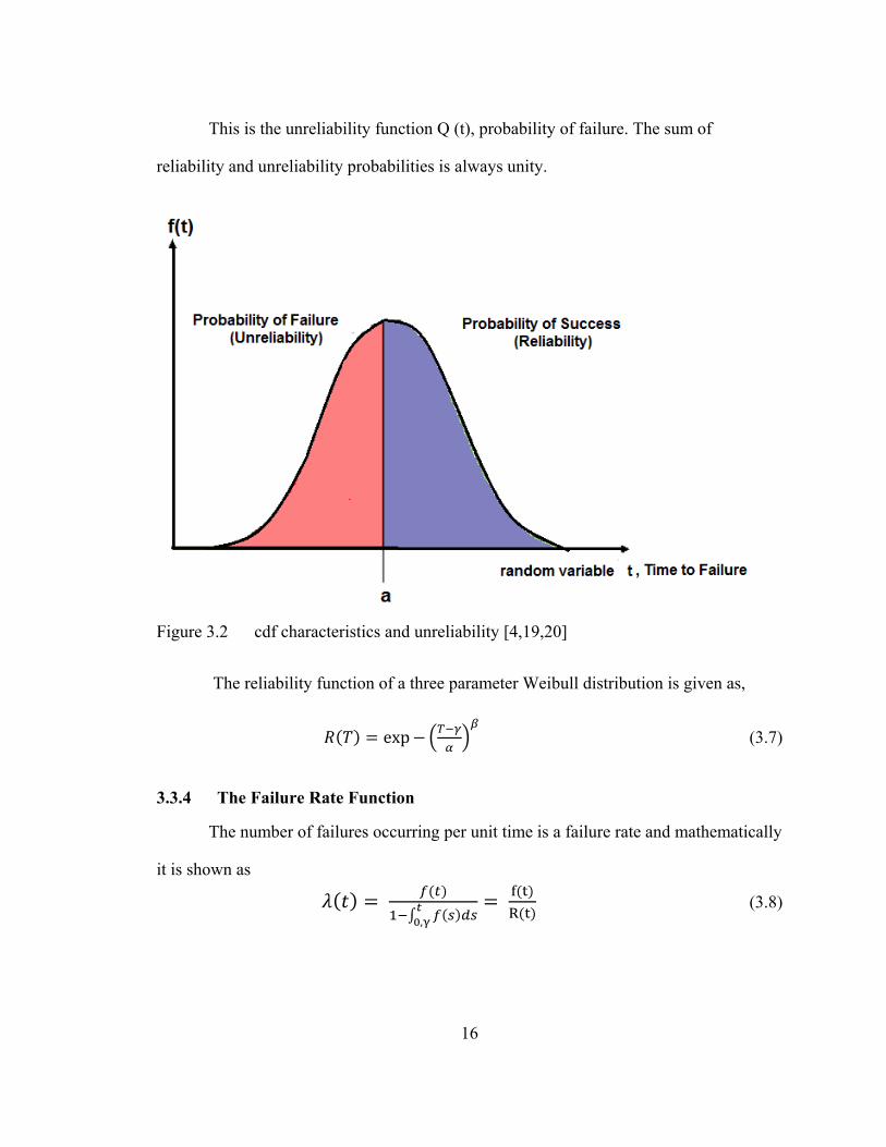
This is the unreliability function Q (t), probability of failure. The sum of

reliability and unreliability probabilities is always unity.

Figure 3.2 cdf characteristics and unreliability [4,19,20]

The reliability function of a three parameter Weibull distribution is given as,

exp (3.7)

3.3.4 The Failure Rate Function

The number of failures occurring per unit time is a failure rate and mathematically

it is shown as

,

(3.8)

17

The Weibull failure rate function, λ (t), is

(3.9)

3.4 Characteristics of Weibull distribution

Due to adaptability of the Weibull distribution, it is mostly used for life time data

analysis. The three parameters, namely scale parameter (α), shape parameter (β) and

location parameter (γ) are important to judge the model of life behaviors. The scale

parameter α is usually a function of the applied voltage when the time is a random

variable. The scale parameter α represents time required for 63.2 % of tested sample to

fail. The shape parameter β or slope of the Weibull distribution is a measure of the time-

to-breakdown. These parameters have influence on the Weibull distribution

characteristics like pdf curve, reliability and failure rate. Following part of the chapter

shows the influence of shape parameter β and scale parameter α on the Weibull

distribution characteristics.

3.4.1 Shape Parameter (β)

The slope of regression line in probability plot is given by the shape parameter, β.

3.4.1.1 Effect of β on the pdf

From the figure 3.3 we can see that, for 0 ≤β ≤1, f (t) looks convex in shape and

it decreases monotonically [t→0, f (t) → ∞] [t→∞, f (t) → 0] and for β > 1, f (t) increases

as t tends to maximum value of pdf and it decreases subsequently.

18

Figure 3.3 The effect of the Weibull shape parameter on the pdf [19,20]

19

3.4.1.2 Effect of β on the cdf and reliability function

Figure 3.4 shows effect of β on the cdf when scale parameter has fixed value,

Figure 3.4 The effect β on the cdf [19,20]

Figure 3.5 shows the effect of different values of β on the reliability plot; from

figure it’s clear that reliability decreases sharply and has convex shape for values 0 <β <1

and even for β=1, but reliability decreases less sharply For β.>1 , reliability decreases as

time increases. As wear out sets in, the curve goes through an inflection point and

decreases sharply.

20

Figure 3.5 The effect β on the reliability [19, 20]

3.4.1.3 Effect of β on the failure rate

The value of β has a marked effect on the failure rate of the Weibull distribution.

Figure 3.6 showed that with β < 1 exhibit a failure rate that decreases with time, β = 1

have a constant failure rate and β > 1 have a failure rate that increases with time.

21

Figure 3.6 The effect β on the failure rate [19,20]

The value of shape parameter describes the failure methodology. If shape

parameter β < 1, then failure is due to reasons like Burn-in testing and/or environmental

stress screening are not well implemented, troubles in the production line, inadequate

quality control, packaging and transit problems. If shape parameter β > 1, then failure is

due to wear -out type failure means natural aging.

3.4.2 Scale Parameter (α)

Effect of change in scale parameter on distribution is like change of the abscissa If

α is increased then the distribution gets stretched out to the right and its height decrease If

α is decreased then the distribution gets pushed towards the right and its height increases.

22

Figure 3.7 The effect α on the pdf [19,20]

In both the cases shape and location remains the same.

23

CHAPTER IV

BREAKDOWN IN SOLID DIELECTRICS

4.1 Introduction

Solid insulation plays a significant role in designing of the high voltage

equipment. Solid insulation provides the insulation between live parts, and it helps as a

mechanical support to the system. A good quality dielectric should have low dielectric

loss, high mechanical strength, should be free from gaseous inclusion, and moisture, and

be resistant to thermal and chemical deterioration. Solid dielectrics have higher

breakdown strength internally compared to liquids and gases.

The breakdown of solid dielectrics depends upon the magnitude of voltage as well

as the time for which voltage is applied. The strength of the solid dielectrics depend upon

many factors like ambient temperature, humidity, duration of test, impurities or structural

defects, type of voltage applied means ac , dc or impulse , pressure etc. The breakdown of

solid dielectrics depends upon magnitude of voltage applied as well as time for which

voltage is applied. Figure 4.1 shows the mechanism of failure. The various mechanism of

breakdown of solids is divided according to time scale and they are as following [21].

Intrinsic Breakdown

Electromechanical Breakdown

Thermal Breakdown

Electrochemical Breakdown

24

Figure 4.1 Mechanism of failure and variation of breakdown strength verses time of stressing [21]

4.2 Intrinsic Breakdown

The mechanism that leads to a sudden loss of insulating capabilities even after a

short period of stressing, without appreciable preheating and without partial discharges, is

called intrinsic breakdown [22]. When voltages are applied only for short durations of the

order of 810 s the dielectric strength of a solid dielectric increases very rapidly to an upper

limit called the intrinsic electric strength. The intrinsic strength mainly depends on

structural design of material and temperature [23].

25

Intrinsic breakdown depends upon the presence of free electrons which are

capable of migration through the lattice of the dielectric. Usually, a small number of

conduction electrons are present in solid dielectrics, along with some structural

imperfections and small amounts of impurities. The impurity atoms, or molecules or both

act as traps for the conduction electrons up to certain ranges of electric fields and

temperatures. When these ranges are exceeded, additional electrons in addition to trapped

electrons are released, and these electrons participate in the conduction process. Based

on this principle, two types of intrinsic breakdown mechanisms have been proposed [23].

4.2.1 Electronic Breakdown

Intrinsic breakdown occurs in time of the order of 10-8 s and therefore is assumed

to be electronic in nature. The initial density of conduction (free) electrons is also

assumed to be large, and electron-electron collisions occur. When an electric field is

applied, electrons gain energy from the electric field and cross the forbidden energy gap

from the valence band to the conduction band. When this process is repeated, more and

more electrons become available in the conduction band, eventually leading to

breakdown [23].

26

Figure 4.2 Schematic energy level diagram for an amorphous dielectric [21]

4.2.2 Avalanche or Streamer Breakdown

This is similar to breakdown in gases due to cumulative ionization. Conduction

electrons gain sufficient energy above a certain critical electric field and cause liberation

of electrons from the lattice atoms by collision. Under uniform field conditions, if the

electrodes are embedded in the specimen, breakdown will occur when an electron

avalanche bridges the electrode gap.

An electron within the dielectric, starting from the cathode will drift towards the

anode and during this motion gains energy from the field and loses it during collisions.

When the energy gained by an electron exceeds the lattice ionization potential, an

additional electron will be liberated due to collision of the first electron. This process

repeats itself resulting in the formation of an electron avalanche. Breakdown will occur,

when the avalanche exceeds a certain critical size [23].

In practice, breakdown does not occur by the formation of a single avalanche

itself, but occurs as a result of many avalanches formed within the dielectric and

extending step by step through the entire thickness of the material [23].

27

4.3 Electromechanical Breakdown

In a dielectric material charges of opposite nature are induced on the two opposite

surfaces when it is subjected to an electric field. Because of opposite charges force of

attraction is developed and material is subjected to electrostatic compressive forces.

Material breakdowns when these electrostatic compressive forces exceed the mechanical

compressive strength. If the thickness of the specimen is d0 and is compressed to

thickness d under an applied voltage V, then the electrically developed compressive

stress is in equilibrium if

ln (4.1) Where,

is permittivity of free space

is permittivity of the material

Y is the Young’s modulus

ln (4.2)

Usually, mechanical instability occurs when 0.6

Substituting this Eq.4.2, the highest apparent electric stress before breakdown,

0.6 (4.3)

The above equation is only approximate as Y depends on the mechanical stress.

Also when the material is subjected to high stresses the theory of elasticity does not hold

good and plastic deformation has to be considered [21, 23, 24].

28

4.4 Thermal Breakdown

Most dielectrics show increasing electrical conductivity and decreasing thermal

conductivity as the temperature increases. For this reason, breakdown at high

temperatures tends to thermal in nature [40].

When an electric field is applied to a dielectric, conduction current however small

it may be, flows through the material. The conduction current and dielectric losses due to

polarization heats up the specimen and the temperature rise. The heat generated is

transferred to the surrounding medium by conduction through the solid dielectric and by

radiation from its outer surfaces. The heat generated is equal to the heat used to raise the

temperature of the dielectric, plus the heat radiated then equilibrium is reached.

The heat generated under dc stress E is given as

(4.4)

Where,

is the dc conductivity of the specimen

Under ac fields, the heat generated

. ∗ (4.5)

Where,

f= frequency in Hz,

loss angle of the dielectric material,

The heat dissipated rW is given by

(4.6)

Where,

Cv= specific heat of the specimen,

T = temperature of the specımen,

29

K = thermal conductivity of the specimen,

t = time over which the heat is dissipated.

Equilibrium is reached when the heat generated Wdc or Wac becomes equal to the

heat dissipated (Wr). In actual practice there is always some heat that is radiated out. If

Wdc or Wac is greater than Wr then system undergo breakdown.

Figure 4.3 Thermal stability or instability under different applied fields [21]

Above Figure 4.3 shows the thermal instability condition. As temperature of

system increase, even conductivity increase. When rate of heating exceeds rate of

cooling, specimen undergo breakdown. From Figure we can see that field 1 is in

equilibrium at temperature T1, field 2 is in state of unstable equilibrium at T2 and field 3

does not reach the state of equilibrium at all [21, 23].

4.5 Erosion Breakdown

Solid dielectrics have voids within the material or boundaries between electrode

and solid dielectric .These voids are filled with the medium of lower breakdown strength,

30

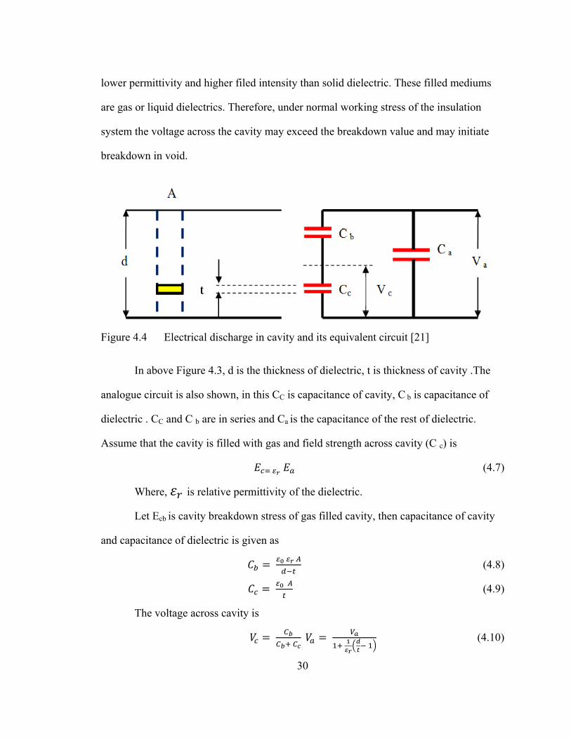
lower permittivity and higher filed intensity than solid dielectric. These filled mediums

are gas or liquid dielectrics. Therefore, under normal working stress of the insulation

system the voltage across the cavity may exceed the breakdown value and may initiate

breakdown in void.

Figure 4.4 Electrical discharge in cavity and its equivalent circuit [21]

In above Figure 4.3, d is the thickness of dielectric, t is thickness of cavity .The

analogue circuit is also shown, in this CC is capacitance of cavity, C b is capacitance of

dielectric . CC and C b are in series and Ca is the capacitance of the rest of dielectric.

Assume that the cavity is filled with gas and field strength across cavity (C c) is

(4.7)

Where, is relative permittivity of the dielectric.

Let Ecb is cavity breakdown stress of gas filled cavity, then capacitance of cavity

and capacitance of dielectric is given as

(4.8)

(4.9)

The voltage across cavity is

(4.10)

31

Thus, the voltage across the dielectric which will initiate discharge in the cavity is

1 1 (4.11)

A void in the material is mostly almost spherical in practice so the internal field

strength of the spherical cavity is given by

(4.12)

For ≫ , and E is average stress in dielectric. Cavity may breakdown when

Vc cavity voltage reaches breakdown value V+ of the gap t under an applied voltage V a.

The sequence of breakdowns under sinusoidal alternative voltage is shown in

Figure 4.5. The red curve shows the voltage that would appear across the cavity if it did

not break. As V c reaches value V+, discharge takes place, the voltage V c collapses and

the gap quenches. The voltage across the cavity then starts growing again until it reaches

V+, when new discharge occurs. Therefore, several discharges may take place during the

positive cycle of the applied voltage. Also, during negative cycle of applied voltage,

several discharges take place when cavity voltage V c reaches V-.

32

Figure 4.5 Sequence of cavity breakdown under alternating voltages [21]

Surface of the insulation provides instantaneous anode and cathode when gas in

the cavity breakdowns. Few of electrons imposed on anode are so active to break

chemical bonds of the insulation surface. Insulation gets damaged when cathode

bombardments by positive ions causes increase of surface temperature and generate local

thermal instability. In addition channels and pits are formed and they elongate through

insulation by edge mechanism. Erosion takes place in the beginning over a large area

when discharges occur on the insulation surface. Surfaces became rough because of

erosion and slowly break through the insulation and at some point will give rise to

channel propagation and tree like growth through the insulation [21,23,24].

Previous studies show that the failure mechanism of tested samples of magnet

wire under ac voltage show multi failure mode of operation, namely partial discharge and

aging caused by electrical stresses. On the other hand, aging at dc voltage shows that the

failure of the tested samples is attributed basically to thermal and electrochemical

breakdown. In this study of Magnet wire MW 16-C the partial discharge / erosion

33

breakdown is main cause of failure of wire along with electrical stresses for ac voltages

and under dc voltage breakdown occurred because of thermal instability. So, this chapter

describes impact of these physical quantities on breakdown of magnet wire.

34

CHAPTER V

LITERATURE REVIEW

5.1 Introduction

Insulation of system is of a prime importance in designing of electrical

equipment. For reliable design of electrical equipment, continuous efforts have been

made to study ageing mechanism of electrical insulation system and to formulate

mathematical model to describe the ageing process under the dominating factor of

influence [25].

The two well know approaches for studying the electrical breakdown of

polyimide insulating material are phenomenological studies and statistical analysis of

failures of electrical insulation due to presence of degrading stresses, such as electrical,

thermal and other environmental factors. The complete understanding of breakdown

mechanism is required in phenomenological studies. Physical and/or chemical tests are

performed on the insulating material in phenomenological studies and then mathematical

model functional with life time is developed. In approach of statistical analysis, alike

specimens of solid insulation are subjected to life tests to measure time to breakdown of

samples. Weibull probability distribution is used to model the data of life tests [26].

To set up a correlation between aging process and the stresses causing it, to

propose models, and to validate them is the main objective of aging studies. An

accelerated aging process is the key for all this and the results of accelerated aging

studies are applied to normal operating conditions. Due to time limitation, realistic long-

35

term tests at working stresses are not achievable. For example, underground transmission

cables are designed for forty years of service. Hence, it’s very helpful for designer

engineers to envisage end of life with certain degree of accuracy in small time duration

by accelerating the aging process. This is the reason that the accelerated aging tests are

generally accepted methods for estimating the service-life and other characteristics of

solid electrical insulation [28].

Accelerated aging test is performed mainly with one or a few dominant stress

parameters, while the others are kept near operating stress. Single stress and multi-stress

life models are mainly used to estimate the lifetime model of the insulation.

5.2 Single Stress Life Models

Voltage and Temperature are two important factors used for the accelerated aging

test. There are two single life stress models namely life models for electrical stress and

life models for thermal stress. Life models for electrical stress include the inverse power

law model and exponential law model and that for thermal stress is the Arrhenius model

[27].

5.2.1 Life Models for Electrical Stresses

The electrical aging models describe aging in any insulation system that

experiences an electrical field. Electrical stress is the major factor that causes degradation

of electrical insulation of the system. Two major models relating the test stress with the

time to failure are universally accepted: the inverse power model and the exponential

model. These models are empirical models as they neither take into account the exact

type of ageing process, e.g., whether partial discharges are present or not nor they

36

consider the system structure, like the particular electrode configuration. Though, the

models have demonstrated to fit reasonably well with experimental data [27,29,30].

5.2.1.1 Inverse Power Law

In the aging studies under electrical stresses the inverse power law is the most

frequently used model and is given as,

(5.1)

log log log

Where, L is the time -to-breakdown and is usually a Weibull scale parameter α at

63.2 % probability, or any other percentile, V is applied voltage, and k,n are constants to

be determined for the specific tested material . By plotting the graphs with the time to

breakdown for corresponding voltage stress in logarithm plot, a straight line is obtained,

which determines the constant parameters. The inverse law is valid if plot fits straight

line [27,29,30].

5.2.1.2 Exponential Law

The other than Inverse power law the best know model of lifetime calculation is

Exponential law and is given as,

exp (5.2)

log log

Where, L is time to failure, V is applied voltage, and c and k are constants to be

found from experimental data. Again, the validity of exponential model is checked by

plotting the data points on semi-log paper and plot should be straight line to be valid

[27,29,30].

37

5.2.2 Life Model for Thermal Stresses

One of the major factors that decide the rating of electrical insulation is its

thermal capability. The thermal capability of insulating material is found out by thermal

aging test. Thermal aging, i.e. aging due to elevated temperature, is associated with

thermally activated rate processes. The backbone of the thermal aging studies is

Arrhenius relation. Dependency of chemical reaction rate on the temperature is shown by

this Arrhenius equation.

exp (5.3)

Where, L is time-to-breakdown, T is absolute temperature, A and B are constants

determined by the activation energy of the reaction. Similar to the voltage aging models,

when log life is plotted against reciprocal of absolute temperature (l/T), a straight line

results [27,29,30].

5.3 Multi stress Life Models

Multi stress models are of special significance in recent growth in the aging

studies on electrical insulation. In multi stress life tests, system is subjected to more than

one stress at a time. When an insulating system is subjected to more than one aging factor

interactions may come into play. There are two main types of interaction direct

interaction and indirect interaction. In direct interaction factors act simultaneously and

indirect interaction essentially remains the same whether the aging factors are applied

sequentially or simultaneously. An example of direct interaction is oxidation - both

oxygen and elevated temperature is needed at the same time to give synergy effect.

Indirect interaction may be the result of mechanical and electrical stress. Micro voids

created by the mechanical stress may give rise to partial discharge activity. Interaction

38

causes the ageing process to proceed at a faster rate compared to the sum of the

corresponding single stress rates. In which way principal ageing models for combined

thermal-electrical stress take synergy effects into account [30]. Multi stress models relate

the connections of electrical and thermal stresses by using multiplicative law. The life

under combined stresses is linked to product of life under single stress in multiplicative

law. The formula derived from the multiplication of the inverse power law model and

Arrhenius relationship and is given as,

, (5.4)

Above equation (5.4) is the basis for Simoni’d and Ramu’s electrical-thermal life

models. The other model that expresses relation between electrical exponential model and

Arrhenius relationship is given as,

, (5.5)

Equation 5.5 is the origin of the Falo’s model. Montanari et.al presents one more

model based on the inverse power law. A concise outline of all electrical- thermal life

models of Simoni, Ramu, Fallou, and probabilities model of Montanari are discussed in

this chapter along with electrical-thermal-frequency life models.

5.3.1 Simoni’s Model

The Simoni’s model shows that the insulation life-time at a specific voltage and

temperature, in relative terms with respect to a reference life-time determined at room

temperature and an electrical stress and is given by [25].

, exp B∆ (5.6)

39

Where, t0 is the time-to-breakdown at room temperature, V=V0 ∆ ,

and B and n are constants to be determined experimentally [33].

5.3.2 Ramu’s Model

The Ramu’s model is obtained from a multiplication of classical single stress

laws, and is given by [26],

, exp B∆ (5.7)

Where, K (T) = exp (K1-K2∆ ), n (T) = exp (n1-n2∆ ), K1, K2, n1, and n2 are

constants.∆ is the same as that defined for the Simoni’s model [34].

5.3.3 Fallou’s Model

Fallou projected a semi-empirical life model which is stood on the exponential

model for electrical aging,

, exp (5.8)

Where, C, A, and B are electrical stress constants and must be determined

experimentally from time-to-breakdown curves at constant temperatures [37].

5.3.4 Montanari’s Probabilistic Model

The relation between the failure probability p to the insulation life L p is given by

the probabilistic life model of combined electrical and thermal stresses of Montanari et al.

It is based on substituting the scale parameter in the Weibull distribution with the life

using inverse power law. For a given time-to-breakdown probability p, the probabilistic

model is given as,

,

ln 1 (5.9)

40

Where, Lp is a lifetime at probability p, Ls is a time-to-breakdown at reference

voltage Vs, and β is the shape parameter [26, 35].

5.3.5 Electrical-Thermal Model

At Mississippi State University High Voltage Laboratory, electrical-thermal

model is developed when insulation of magnetic wire is stressed with voltage and

temperature performing accelerated aging test. The Electrical-Thermal model is given as,

, exp (5.10)

Where, L is the life-time at 63.2% probability of breakdown, V is the applied

voltage, T is the temperature, and C, A, and B are constants to be determined by

analyzing the combined voltage-temperature life data.

Natural logarithm plot is used to liberalize the equation 5.10. The life-time versus

the stress, either voltage V or temperature T, and keeping the other one constant is plotted

to find a set of linear curves. The slope of the linearized Arrhenius equation when the

voltage is constant is given by B and the slope of the exponential electrical function

model when the temperature is constant is A [2,26].

Assume life-time is a random variable then the model shown by equation (5.10)

can be transformed into a probabilistic model by setting the scale parameter of the

Weibull distribution equals to L (V,T). The time-to-breakdown of the electrical insulation

under combined electrical and thermal stresses is statistically distributed according to a

Weibull distribution, then the Weibull pdf can be written as,

, exp (5.11)

41

Where, L is the life-time at 63.2% probability of breakdown, V is applied the

voltage, T is the temperature and K, B and n are constants to be determined by analyzing

the combined voltage- temperature life data [2, 26].

5.3.6 Electrical-Thermal-Frequency Model

The life time model due to thermal and electrical stresses at ac voltage and dc

voltage for industry frequency is discussed till now. The insulation material like

insulation in the inverter-fed motors, no longer experiences a traditional sine wave

voltage that is a steady state condition, but instead experiences a pulse-wave with

significant harmonics and transients. The work was done at Mississippi State University

using high frequency square pulse voltage as an electrical stress to obtain the lifetime

model of magnet wire insulation. S. Grzybowski et al. deduced the frequency-electrical-

thermal life model based on the application of high frequency pulse voltage. The

electrical-thermal- frequency life-time model is a general multi stress model, which

includes the effect of voltage magnitude, temperature and frequency. It is a probabilistic

life-time model and is given by

, , exp (5.12)

Where t time-to-breakdown at 63.2% probability of failure, for specific voltage

and temperature V is the test voltage at the specific temperature, T, T is the test

temperature in Kelvin, f is the frequency in Hz, K, A, m1, and m2 are constants must be

determined experimentally [2, 16,26].

42

CHAPTER VI

EXPERIMENTAL SETUP

6.1 Introduction

Magnet wires are used in machine windings and magnetic wire’s insulation is

stressed by the voltage and temperature. These stresses do degradation of the insulation.

The ability to predict accurately the long-term voltage endurance performance of wire is

essential both to the wire manufacturer and to the motor manufacturer [32].Therefore it is

very important to study the degradation of the insulation stressed by voltage and

temperature. To study the accelerated degradation of machine insulation, a popular

practice used is to study the twisted pair samples under different aging conditions. The

twisted pair samples are prepared according to NEMA standard. This standard specifies

the number of twists and the tension to be applied for making the twisted pair depending

on the size of the wire. In this experiment the magnet wire tested was NEMA MW 16-C,

wire size was 14 AWG, diameter of 0.0641 inches nominal.

6.2 Dielectric Test System

The accelerated degradation of the insulation of magnetic wire was performed

using the Dielectric test system (DTS) as shown in Figure 6.1 .The DTS-1500 is an

integrated test system used to study the failure mechanism of the machine winding

insulation by simulating the electrical and thermal stresses under controlled and

accelerated conditions. The DTS-1500 test system is designed to vary and monitor

electrical and thermal test parameters for up to five samples simultaneously.

43

The Dielectric test system was set up with

An ac source test system for accelerated degradation testing of twisted pair

samples that can be varied from 0 to 12 kV

A 10 kV dc source test system for accelerated degradation testing of

twisted pair samples

A convection air-circulating oven whose temperature can go up to 260OC

starting from room temperature to aid testing at a controlled and elevated

temperature of twisted pair magnetic wire samples. Five samples can be

aged simultaneously in the oven.

For an ac system, an oscilloscope which was calibrated with 1:1000 ratio

using a voltage divider.

A timer that counts the time to breakdown for the samples.

44

Figure 6.1 The Dielectric Test System

45

6.3 Sample Preparation

According to NEMA standard to study of the electrical insulation system for a

machine winding a twisted pair method is used. The twisted wire sample is as shown in

Figure 6.2.

Figure 6.2 Twisted Pair sample on DTS tray [16]

NEMA standard specifies the number of twists required for the twisted wire

samples. A specimen of wire is formed into a “U” shape, and the two legs are twisted

together the number of 360o rotations specified in Table 6.1 to form an effective length of

4.75±0.25 inches (121 mm±6 mm). The total tension on the two legs and the total number

of rotations is shown in Table 6.1 [16, 38].

In the DTS largest wire diameter can be used is a 14 AWG size round conductor.

More than 4 full twists are not allowed with a tension force of 12 pounds to magnetic

wire according to NEMA standard. A device that counts the number of twists and puts

consistent tension on the wire during the twisting process, called twist fabricator, is used

to prepare samples.

46

Table 6.1 Tension and rotation of Twisted samples [16, 38 ]

AWG Size Total Tension on

Specimen (± 2 %)

Total Number of

Rotations

8-9 * 24 lb (107 N) 3

10-11 24 lb (107 N) 3

12-14 12 lb(53 N) 4

15-17 6 lb (27 N) 6

18-20 3 lb (13 N) 8

21-23 1.5 lb (7 N) 12

24-26 340 gm (3.3 N) 16

27-29 170 gm (1.7 N) 20

30-32 85 gm (0.8 N) 25

33-35 40 gm (0.4 N) 31

36-37 20 gm (0.2 N) 36

.

Figure 6.3 shows the dielectric twist fabricator used to prepare the samples

according to the NEMA standard for a 14 AWG size round conductor. After preparation

of the sample, insulation is removed from both ends of the wire for a solid electrical

connection to the high voltage and ground terminal in the DTS.

47

Figure 6.3 Dielectric Twist Fabricator [16]

The two different kinds of samples are made to take measurements. The twisted

pair sample on one side energized with high voltage on one leg and other leg is grounded

but, in one sample two legs on other side is left open floating as shown in Figure 6.4.And

in second kind of sample, the two legs which are of other side of sample are turn round as

shown in Figure 6.5.

Figure 6.4 First Kind of Sample

48

Figure 6.5 Second Kind of Sample

6.4 Accelerating Aging with 60 Hz ac voltage

For accelerated aging of insulation of magnetic wire constant stress test procedure

is used. In constant stress test the applied voltage is held constant and time-to-breakdown

is noted. The NEMA MW-16 C wire is used for the experiment which has temperature

rating of 240OC. Figure 6.6 shows the experimental set up to obtain time-to-breakdown

of NEMA MW 16-C insulation at various 60 Hz ac stress level.

Figure 6.6 Setup Circuit for accelerated aging at 60 Hz ac voltage [16]

The main breaker connected to the ac source trips the interlock when a sample is

broken by sensing high current flow through the short circuited magnet wire which stops

the timer. After breakdown the entire system was shut down in order to determine which

sample was broken. All samples were removed from the oven and were tested using

49

insulation tester to find the broken sample. The insulation tester used is shown in

Figure 6.7. It is basically a mega ohm-meter which applies high dc voltage across the

twisted pair samples and measures the insulation resistance. If the sample is broken the

meter reads very low resistance as high voltage cannot be applied across the short

circuited sample. Using this we can separate out broken sample from unbroken samples.

The unbroken samples are again placed back into the oven and the system is again

restarted.

Figure 6.7 Insulation Tester : Meg Ohm Meter

The accelerated aging are conducted over the 60 Hz ac effective voltage range

from 1.5 kV to 3 kV at room temperature of 23OC, and from 1.5 kV to 3 kV at 70 O C and

190OC, using a minimum of four samples of first kind and second kind at each test

condition.

6.5 Accelerating Aging with 10 kV dc voltage

Figure 6.8 shows the experimental test set up used for accelerated aging of

insulation of magnet wire. Magnet wire MW 16-C, thermal rating 240OC is used and it is

50

stressed with 10 kV dc voltages at room temperature and at elevated temperature and

time-to-breakdown is noted down.

Figure 6.8 Set up diagram for 10 kV dc for accelerated aging of magnet wire

The accelerated aging is conducted at 10 kV dc voltages at room temperature of

23OC and 190OC using a minimum of four samples of second kind at each test condition.

51

CHAPTER VII

TEST RESULTS

7.1 Accelerated Degradation with ac 60 Hz Voltage

7.1.1 Weibull Distribution

Two parameter Weibull distributions are used for analysis of time to breakdown.

The two parameter Weibull pdf is given as,

exp (7.1)

Where, α is the 63.2% nominal life time, and β is the shape or variance parameter.

The time to breakdown value is obtained for a minimum of four samples at the particular

voltage level, ranging from 1.5 kV to 3 kV.

The Weibull plots in Figure 7.1 through Figure 7.4 show the plots for the twisted

pair of samples of first kind and Figure 7.5 through Figure 7.8 shows the Weibull plots of

the twisted pair of sample of second kind. From the graphs, it is obvious that the shape

factor β increases with test voltage, while being nearly invariant with respect to

temperature. Such voltage dependence indicates a change in the physical aging process

when the test voltage is increased from 1.5 kV to 3 kV. Table 7.1 and Table 7.2

represents time to breakdown (63.2% probability) values obtained from the Weibull

distribution plot from 1.5 kV to 3 kV for temperatures of 23OC, 70OC, and 190OC,

respectively.

52

Figure 7.1 Weibull plots of 60 Hz breakdown voltage probability of twisted samples of first kind aged at 1.5 kV at 23OC , 70OC and 190OC

53

Figure 7.2 Weibull plots of 60 Hz breakdown voltage probability of twisted samples of first kind aged at 2 kV at 23OC , 70OC and 190OC

54

Figure 7.3 Weibull plots of 60 Hz breakdown voltage probability of twisted samples of first kind aged at 2.5 kV at 23OC , 70OC and 190OC

55

Figure 7.4 Weibull plots of 60 Hz breakdown voltage probability of twisted samples of first kind aged at 3 kV at 23OC , 70OC and 190OC

56

Figure 7.5 Weibull plots of 60 Hz breakdown voltage probability of twisted samples of second kind aged at 1.5 kV at 23OC , 70OC and 190OC

57

Figure 7.6 Weibull plots of 60 Hz breakdown voltage probability of twisted samples of second kind aged at 2 kV at 23OC , 70OC and 190OC

58

Figure 7.7 Weibull plots of 60 Hz breakdown voltage probability of twisted samples of second kind aged at 2.5 kV at 23OC , 70OC and 190OC

59

Figure 7.8 Weibull plots of 60 Hz breakdown voltage probability of twisted samples of second kind aged at 3 kV at 23OC , 70OC and 190OC

The time to breakdown for different probability of breakdown voltage are

calculated from the given Weibull distribution plot at each voltage stress for different

temperatures. Changes in the aging process with changes in voltage levels are also shown

by the summarized V-t lifetime graphs and are plotted according to the inverse power law

and Arrhenius equation. The life time of the samples decreases with increase in the stress

levels.

60

Table 7.1 Time to breakdown (63.2 % probability ) for MW 16-C insulation at different voltages level of First kind of samples

Applied

Voltage(kV)

Time to Breakdown (63.2 % Probability )

23 OC 70 OC 190 OC

1.5 52.95 53.2 29.81

2 27.86 23.31 19.50

2.5 16.70 12.96 9.40

3 8.23 6.99 6.65

Table 7.2 Time to breakdown (63.2 % probability ) for MW 16-C insulation at different voltages level of Second kind of samples

Applied

Voltage(kV)


23 OC 70 OC 190 OC

1.5 108.36 47.08 25.44

2 45.50 30.76 14.43

2.5 29.61 14.97 9.96

3 20.66 8.44 5.66

7.1.2 Inverse Power Law

Using values of Table 7.1 and Table 7.2 the graph is plotted and it fits the inverse

power law; Inverse power law is given as,

(7.2)

Where, L is the time -to-breakdown and is usually a Weibull scale parameter α at

63.2 % probability, or any other percentile, V is applied voltage, and k,n are constants to

be determined for the magnet wire MW 16-C for Polyimide insulation.

61

The results of time to breakdown fit very well to inverse power law as shown

Figure 7.9 and Figure 7.10, and the value of exponent n shows the effect of stress on the

insulation.

Figure 7.9 Measured time to breakdown (Hrs) at 63.2 % probability of breakdown voltage at each voltage stress , plotted according to the inverse power law for First kind of Twisted pair samples

62

Figure 7.10 Measured time to breakdown (Hrs) at 63.2 % probability of breakdown voltage at each voltage stress , plotted according to the inverse power law for Second kind of Twisted pair samples

From the graph, using the inverse power law, the lifetime model of MW 16-C

insulation is obtained, which is presented in Table 7.3.

63

Table 7.3 Inverse power model of MW 16-C at different temperature

Agin

g

Temperature

Inverse Power Model

First Kind of Sample Second Kind of Sample

23 O

C 149.25 . 277.77 .

190

O C 96.15 . 57.14 .

7.1.3 Arrhenius Relation

The aging mechanism is also shown by Arrhenius plots and Arrhenius equation is

given as,

exp (7.3)

Where, L is time-to-breakdown, T is temperature in K, A, and B are constants

determined by the activation energy of the reaction. It is confirmed that the test voltage

from 1.5 kV to 3 kV is to reduce the apparent thermal activation energy from

5.17kJ/mole to 1.84kJ/Mole. In general, the temperature dependence of dielectric

properties of polyimide films, as permittivity and dc conduction, is usually governed by

activation energies in the range of 100 to150 kJ/mol. It means that, in this case,

thermally-activated processes of polyimide seem to have a minor effect on the rate of

degradation [16].

Figure 7.11 and Figure 7.12 shows that the results of accelerated aging test fit in

an Arrhenius relation. And Arrhenius relation model is shown in Table 7.4.

64

Table 7.4 Arrhenius relation model for MW 16-C

Agin

g Voltage

Arrhenius Relation Model


1.5

kV 7.6 exp

623.32 0.64 exp

1514.54

3 kV 3.8 exp222.51

0.20 exp1352.18

Figure 7.11 Measured time to breakdown (Hrs) at 63.2 % probability of breakdown voltage at each temperature stress , plotted according to the Arrhenius relation for First kind of Twisted pair samples

65

Figure 7.12 Measured time to breakdown (Hrs) at 63.2 % probability of breakdown voltage at each temperature stress , plotted according to the Arrhenius relation for Second kind of Twisted pair samples

7.1.4 Electrical Thermal Model

The new Electrical-Thermal model shown here is yield by combining Arrhenius

and the inverse power law models for magnet wire MW 16- C.

The model for MW 16-C is given as,

,

(7.4)

Where, L is the lifetime (in hours) at 63.2% of probability of breakdown, V is the

applied voltage, T is the temperature and B, C, and n are the parameters to be determined

for magnet wire MW 16- C.

66

The model is plotted using ALTA software and the Electrical Thermal model plot

is shown in Figure 7.13 with constant stress as Voltage.

Figure 7.13 Electrical-Thermal Model (Plot of Life vs. Temperature (K) keeping voltage stress constant )

67

Estimates of the parameters for twisted pair of samples of First kind and Second

kind is given in Table 7.5

B shows the slope of the life line in a Life vs. temperature plot. It means that B is

the measure of effect of the temperature on the life and n measures the effect of voltage

has on the life. We can see that, higher the value of B, higher the dependency of the life

on the temperature.

Table 7.5 Electrical Thermal Model for MW 16-C

Mod

el Parameter

Electrical Thermal Model


β 12.7 10.5

C 42.57 3.39

n 2.66 2.32

B 425.60 1283.33

7.2 Accelerated Degradation with dc Voltage

The accelerated aging test is conducted on magnet wire MW 16-C when subjected

to 10 kV dc voltages with temperatures 23OC and 190OC The experiment is carried on

Second kind of samples alone. The result of test data is plotted with Weibull Two

parameter Distribution. The Weibull plot is as shown in the Figure 7.14.

The time to breakdown for 10 kV dc is calculated from the given Weibull

distribution plot for different temperatures

68

Figure 7.14 Weibull plots of dc breakdown voltage probability of twisted samples of second kind aged at 10 kV at 23OC ,and 190OC

Table 7.6 Time to breakdown (63.2 % probability ) for MW 16-C insulation at 10 kV dc voltage

Applied

Voltage(kV)


23 OC 190 OC

10 61.60 45.43

69

7.2.1 Arrhenius Relation

Also for the 10 kV dc voltages, the results of time to breakdown fit very well to

Arrhenius relation as shown in Figure 7.15.

Figure 7.15 Arrhenius model for MW 16-C when subject to 10 kV dc voltage

The Arrhenius model for MW 16-C is given as,

21.01 exp . (7.5)

70

7.3 Comparison between ac and dc breakdown mechanism

The aging behavior of MW 16-C Polyimide insulation is investigated at ac and dc

voltages. The statistical distribution of the time-to-breakdown was represented by the

Weibull cumulative probability distribution. The lifetime of the insulation under both ac

and dc electrical stresses with room and elevated temperatures are evaluated using the

Arrhenius relation.

Figure 7.16 Comparison of ac and dc voltages for Arrhenius relation model

The study shows the effect of the temperature on the chemical reaction rate in the

ac voltage and the dc voltage degradation. As value of B is greater in ac than dc,

71

excessive heat is produced in ac than dc; and also effect of temperature is high on life

dependency in ac voltages than dc voltages.

Table 7.7 Comparison of time to breakdown (hrs) between ac and dc voltages

Applied

Voltage(kV)


23 OC 190 OC

10 kV

dc 61.60 45.43

3 kV ac 40.66 5.66

The study shows that insulation aging under ac voltage is much earlier than that

under dc voltage. This is recognized to the extreme heat generated by dielectric losses

and partial discharges in the micro voids. However, under dc voltage the aging process is

sluggish and breakdown results from the reduction of the insulation resistivity due to

ohmic losses [39].

7.4 Comparison between First kind of twisted pair sample and Second kind of twisted pair sample used under ac voltage

From Figure 7.1 through Figure 7.8, it is clear that the Time-to-Breakdown of the

Second kind of twisted pair samples is greater when compared with the Time-to-

Breakdown of the First kind of twisted pair of samples.

In the first and second kind of samples, on one side, one leg is energized with

high voltage and other is grounded. The other side of the first kind of sample is kept open

as shown in Figure 6.4 and in the second kind of sample, the other side of sample is turn

round as shown in Figure.6.5. In the first kind of sample as the legs on other side are

72

sharp points, so they are more prone to more electrical stress at the end. In second kind of

samples, electrical stress is reduced by making the ends of the legs round shaped. To

achieve the highest strength the sample is so designed that stress is in the center of the

dielectric and lower at the edges to cause discharge in medium. In the first kind of

samples, sample broke at the edge of the sample where as in the second kind of sample, it

broke at middle of the sample. The second kind of twisted sample is superior to that of

the first kind of samples.

73

CHAPTER VIII

CONCLUSION

The idea behind this work is to verify the electrical thermal model for the magnet

wire MW-16 C when stressed under ac voltage and high temperature. In the thesis, 60 Hz

ac breakdown measurement and dc breakdown measurements are performed on the

NEMA MW-16 C insulation. The accelerated test is carried out for ac voltages ranging

from 1.5 kV to 3 kV and under different temperatures (23OC, 70OC and 190OC).The main

conclusion from measurement are as follows

The time to breakdown for 60 Hz ac is modeled with combining the

Weibull distribution of failure data with the inverse power law and the

Arrhenius relation with respect to test voltage and temperature.

Electrical Thermal life model is verified for 60 Hz ac voltage

,

(8.1)

The estimated parameters for MW 16-C are given in Table 7.5

The time to breakdown for 10 kV dc is modeled with combining the

Weibull distribution of failure data with the Arrhenius relation with

respect to temperature.

The insulation aging under ac voltage is much earlier than that of under dc

voltage for MW 16-C.

74

Breakdown in ac is due to partial discharge and aging caused by electrical

stress, and in dc breakdown is due to thermal and electro-thermal

breakdown.

Second kind of samples are much superior than that of first kind as they

are designed such that the stress is in the center of the dielectric and lower

at the edges to cause discharge in medium.

The possible future work could be;

Accelerated degradation test under dc voltage with more than

10 kV dc voltage applications to find out Electrical-Thermal model

under dc voltage.

The accelerated aging of MW 16-C with ac superimposed on dc

voltage.

75

REFERENCES

[1] G.Montanari, “Bringing an Insulation to Failure: the role of space charge”, IEEE Transactions on Dielectrics and Electrical Insulation, Vol. 18, No. 2; April 2011

[2] N. Kota, “Analysis of Magnet Wire Lifetime Characteristics Frequency Pulsating” Master of Science Dissertation, Mississippi State University, 2005.

[3] S. Grzybowski E. A. Feilat P. Knight L. Doriott, “Breakdown voltage behavior of PET Thermoplastic at DC and AC voltages”, Proceedings of 11th International Symposium on High Voltage (ISH99), London, UK, August 23-27, 1999, pp. 308-311.

[4] S.Bandaru, “Effect of High Frequency Pulse Voltages and High Temperature on the Lifetime Characteristics of Magnet wires” Master of Science Dissertation, Mississippi State University, 2004

[5] L. S. Nelson, A. Wayne, “Accelerated Testing: Statistical Models, Test Plans, and Data Analyses”. New York: John Wiley & Sons, Inc., 1990.

[6] E. Ildstad, and S. R. Chalise, “AC Voltage Endurance of Polyimide Insulated Magnet Wire,” Submitted for Conference on Electrical Insulation and Dielectric Phenomena (CEIDP, 2009), 18-21 Oct., Virginia, USA.

[7] http://www.superioressex.com/magnetwire.aspx

[8] http://www.nema.org/prod/ins/magnet/

[9] http://www.calfinewire.com/index.php?id=218

[10] W.T.Shugg, “Handbook of Electrical and Electronic Insulating Materials”, IEEE Press, Shugg Enterprises Inc, 1995

[11] Mark Winkeler, “Magnet Wires Enamels –Which One,” IEEE Electrical Insulation Magazine,” Vol. 7, pp. 61-64, 1993.

[12] E. Sugimoto, “Application of Polyimide Films to the Electrical and Electronic Industries in Japan.” IEEE Electrical Insulation Magazine,” vol-5, pp.15-23, 1989

76

[13] J. Patterson, T. Boyer, and H. Shiozawa, “Encapsulation of Sensors, Solenoid and Transformers with Engineering Thermoplastics”, Proceedings of Electrical and Electronics Insulation Conference, Roesmont, Illinois, September 18-21, 1995 pp. 1-6.

[14] A.Mani, “Study of Partial Discharge activity in Magnet Wires aged by combined stresses,” Master of Science Dissertation, Mississippi State University, 2005

[15] G.Stone , J.Lawless ,” The application of Weibull Statistics to insulation aging test,” IEEE Transactions on Electrical Insulation Vol. EI-14 No.5, October 1979

[16] S. Chalise, “Accelerated aging study of Machine Winding Insulation under AC and High Frequency Pulse Voltages application,” Master of Science Dissertation, Mississippi State University, 2010

[17] http://www.mwswire.com/inschar.htm

[18] M.Morcos, and K.Srivastava, “On the Statistical Testing of Solid dielectrics, “IEEE International Conference on Conduction and Breakdown in Solid Dielectrics, “June 22-25, 1998

[19] http://www.weibull.com/LifeDataWeb/the_weibull_distribution.htm

[20] Weibull++ Life Data Analysis Reference, Version 5.0, ReliaSoft’s, Tucson, Arizona, USA

[21] E. Kuffel, W. S. Zaengl, and J. Kuffel, “High Voltage Engineering: Fundamentals,” Second Edition 2000, Butterworth-Heinemann, Oxford, UK

[22] D. Kind, and H.Karner, “High voltage insulation technology,” Friedr. Vieweg and Sohn, 1985

[23] M.Naidu, and V Kamraju, “High Voltage Engineering,” Tata Mcgraw Hill Publishing Company Limited, third edition

[24] C.Wadhawa, “High Voltage engineering”, New Age International Publishers, second edition

[25] O.Chabra, “Life expectancy of High Voltage Electrical insulation under multi-factor ageing,” IEEE International Symposium on Electrical Insulation, June 5-8, 1994

[26] Eyad Abu-Al-Feilat, “Lifetime Characteristics of Magnet Wires under High Frequency Pulsating Voltage and High Temperature,” PhD Dissertation, Mississippi State University, 2000.

[27] Accelerated Life Testing Reference, Version 6.0, ReliaSoft’s, Tucson, Arizona, USA

77

[28] P. Cygan and J.Laghari, “A Review of Electrical and Thermal multistress aging model,” IEEE International Symposium on Electrical Insulation, June 3-6, 1990

[29] P. Cygan and J. R. Laghari, “Models for Insulation Aging under Electrical and Thermal Multistress,” IEEE transactions on Electrical Insulation, Vol.25 no 5, October 1990

[30] A. Gjaerde, “Multifactor aging model - Origin and Similarities,” IEEE insulation magazine, Vol 13, No1, January/February 1997

[31] G. C. Montanari, L. Simoni, "Aging Phenomenology and Modeling," IEEE Transactions on Electrical Insulation,” Vol. 28, pp. 755-776, 1993

[32] G. Zhang, T. Lin, L. Zhang, G. Wu, “Characteristic of Magnet Wire Based on the Effect of Electrical and Thermal Aging,” Proceedings of IEEE International Conference on Solid Dielectrics, Toulouse, France, Vol. 2, pp. 904-907, 2004.

[33] L.Simoni, “A general approach to the endurance of electrical insulation under temperature and voltage,” IEEE Transactions on Electrical Insulation Vol. EI-16 No .4, August 1981

[34] T. S. Ramu, "On the Estimation of Life of Power Apparatus Insulation under Combined Electrical and Thermal Stress," IEEE Transactions on Electrical Insulation, Vol. EI-20, pp. 70-78, 1985

[35] G. C. Montanari, M. Cacciari, "A Probabilistic Insulation Life Model for Combined Thermal-Electrical Stresses," IEEE Transactions on Electrical Insulation, Vol. EI-20, pp. 519-522, 1985

[36] G.Montanari ,L.Simoni, “ Aging phenomenon and modeling,” IEEE Transactions on Electrical Insulation Vol. 28 No. 5,October 1993

[37] Fallou, C. Burguiere, J. F. Morel, “First Approach on Multiple Stress Accelerated Life Testing of Electrical Insulation”, IEEE 1979 Annual Report Of CEIDP, pp. 621-628.

[38] ANSI/NEMA MW 1000-2003, Revision 3, 2007, Magnet wire, part 3

[39] E.Feilat, “DC and AC Aging Of HV Encapsulated Flyback Transformers,” Proceedings of the 5th WSEAS Int. Conf. on Power Systems and Electromagnetic Compatibility, Corfu, Greece, August 23-25, 2005 (pp491-495)

[40] J.O’Dwyer, “Breakdown in solid dielectrics,” IEEE Transaction on Electrical Insulation Vol.Ei-17 no.6, December 1982

Documents

Lifetime characteristics of Magnet wire MW 16-C under AC