1

Life Cycle Costing with Application to Electric Energy Costing

K. Jo Min, Cameron MacKenzie, and Sarah M. Ryan

( jomin@iastate.edu , camacken@iastate.edu , smryan@iastate.edu )

Section 1. Basic Life Cycle Costing

This chapter is organized as follows. First, we will introduce the concepts and perspectives of

life cycle costing that are explained through engineering design of a product as well as planning

and management of a project. This is followed by the basic mathematical ideas that will lead to

models and analyses. Specifically, in Section 2, we elaborate on the methodology of life cycle

costing that includes calculations with or without inflation, annual equivalent costs, and a

payback approach. An illustrative case example is also provided. Next, in Section 3, we show

how the basic concept can be applied to electric energy costing with environmental

considerations. This section addresses the levelized cost of electricity (LCOE), followed by a

case example, and incremental costs of carbon emission mitigation. Finally, in Section 4, we

make concluding remarks and comment on future directions.

1. Concepts and Perspectives

Life cycle cost is defined to be the sum of all the costs incurred by a product or a project during

its entire life span. Life cycle costing, in turn, is a process of assessing and evaluating economic

performance relevant to a product or a project based on the concept of the life cycle cost. The life

cycle cost is often referred to as the total cost of ownership, and life cycle costing is often viewed

2

as a way to balance initial costs, such as design costs and capital outlays, with subsequent costs

including operations and maintenance costs and the cost of decommissioning.

These concepts and perspectives of the total cost of ownership, along with the balance between

the initial costs and subsequent costs, prevent erroneous selection of alternatives with the lowest

immediate costs. They help various design engineers, project managers, and other decision and

policy makers to choose best alternatives over the entire life cycle.

As life cycle costing has been extensively utilized in several distinct industries, in terms of the

scopes of problems and timelines, there have been developments of several concepts and

perspectives in separate application areas.

A major area of such application has been in engineering design of a product and the choice

among alternative designs. From this perspective, Figure 1 depicts such a problem in four stages.

Low initial cost - high subsequent cost High initial cost - low subsequent cost

Time

Cu

mu

lati

ve

Cost

3

Figure 1. Life-Cycle Stages of a Product for Engineering Design:

2 Designs with Different Cost Characteristics

Figure 1 considers the cumulative costs of ownership for an alternative with a low initial cost and

a high subsequent cost and for an alternative with a high initial cost and a low subsequent cost.

In the short-run (until the curves intersect), the low initial cost alternative is preferred, but in the

long-run, the low subsequent cost alternative is preferred. In addition, the horizontal axis of

Figure 1 illustrates that a product undergoes four stages; namely, design, production, operations

and maintenance, and decommissioning. Details of each stage are as follows.

a. Design: Based on the needs and specifications of the product, a design is conceptually

materialized. The costs of conceptual design, any simulation and prototyping for detailed design,

as well as testing and correction, are all included in this stage.

Alternative designs are also developed with some variations in features, which affect

manufacturing complexities and corresponding costs, as well as operational availability,

maintenance reliability, and decommissioning impacts and costs.

Designs are frequently evaluated via simulation, prototyping, and user consultation. The

cumulative life-cycle cost of a design is shown in Figure 1 in solid line (Design 1) and the cost of

Design Production Operations and Maintenance Decommissioning

4

an alternative design is shown in Figure 1 in dotted line (Design 2). As one can observe, even

though Design 1, relative to Design 2, exhibits low initial costs, the subsequent costs for Design

1, as the product undergoes through the four stages, are higher. Hence, from a life cycle costing

perspective, a design with a low initial cost may be inferior to an alternative design with a high

initial cost on a cumulative cost basis. We do note that there may be other criteria, such as

aesthetics and brands, considered in the final selection of the best alternative that are not

monetized.

b. Production: For the designs under consideration, the corresponding production costs must be

estimated. They include not only the materials and assembly costs and the wages of production

workers, but also the costs of consumables, utilities, and an appropriate share of production

facility and equipment costs.

c. Operations and Maintenance: Operations and maintenance costs are also incorporated into life

cycle costs. They include an appropriate share of wages of all operations and maintenance

personnel and costs in consumables, utilities, and (spare) part inventories.

d. Decommissioning: From the perspective of the aforementioned ownership costs, the cost of

disposal must also be included. For example, for a discrete assembly, such a cost includes the

costs of disassembly, as well as the costs of reuse and recycle minus the benefits of the reuse and

recycle. Some systems will have a positive salvage value instead of a decommissioning cost at

the end of their life cycle.

5

Another major area of such application has been in planning and management of a project,

ranging from software development and utilization to infrastructure construction and usage.

From this perspective, similar to Figure 1’s four stages, we have the following stages.

A. Planning: The costs incurred in this stage include the costs of economic feasibility studies,

costs of design, verification, and validation as needed, and costs associated with benchmarking

and project alternative studies.

B. Construction: Along with each line of a project that is under consideration, the construction

costs include not only the costs of materials and building/programming, but also overhead

associated with the building and programming such as appropriate shares of utilities and

equipment costs. Closeout costs between the construction and usage stage are also included, such

as the training costs of users of the programs as well as the repair and maintenance crew for the

new construction.

C. Usage/Utilization; With respect to each project alternative that is under consideration, the

costs in this stage include not only the routine costs of utilities and the appropriate shares of

wages of employees, but also the costs associated with troubleshooting, spare parts, as well as

software patches as necessary.

D. Decommissioning: For a construction project, the costs in this stage include the costs of

dismantlement as well as the costs associated with environmental, health, and safety mitigation

efforts. For this type of project, the disposal cost of the waste after dismantlement can also be

6

significant. For a software project, the costs of safe and secure disposal of information must be

considered.

Thus far, we have reviewed the concepts and perspectives of life cycle costing through

engineering design of a product as well as planning and management of a project. We now

present the basic mathematical ideas that lead to models and analyses.

2. Methods

This section introduces methods for calculating life cycle costs and illustrates them with an

application to military procurement.

2.1 Life cycle cost calculations

Companies and government agencies are frequently adept at considering design and production

costs when analyzing the costs of new products or systems. These owners or operators may

neglect the operations and maintenance cost. As depicted in Figure 2, on an annual basis, the

operations and maintenance costs can become the largest component of a product’s life cycle

cost, especially for systems that are used past their expected life. Failing to consider the

operations and maintenance costs when determining whether to develop, design, produce, or

procure a system, or when comparing different systems, may lead to a substantial underestimate

of the costs and result in the wrong investment decision.

7

Figure 2 Elements of life cycle cost

A life cycle cost analysis considers the annual costs for each year of the system beginning with

the design and continuing through the end of the system’s life when the system is

decommissioned or disposed. Cost overlap will frequently occur among each category of the life

cycle. For example, one year may contain both design costs as well as production costs. Another

year may contain both production costs and operation and maintenance costs.

Life cycle cost analysis typically aggregates the annual costs over the life of the system into a

single number using concepts based on the time value of money. The interest or discount rate i is

used to calculate the present value of annual costs in year 0 or the current year. The life cycle

cost (LCC) is calculated using the present value formula over the life of the system:

𝐿𝐶𝐶 = ∑𝐶𝑡

(1+𝑖)𝑡𝑇𝑡=0 (1)

where Ct is the annual cost in year t and T is life of the system in years. Present value

calculations usually follow the convention that cash inflows (i.e., revenue) are positive numbers

and cash outflows (i.e., costs) are negative numbers. However, life cycle cost calculations may

8

follow the reverse: Ct > 0 signifies costs and Ct < 0 signifies cash inflows (e.g., a salvage value).

Since life cycle costs do not consider the benefits or revenue gained from fielding a system apart

from the potential salvage value of selling the system at the end of its useful life, LCC in

Equation (1) is a positive number.

2.2 Life cycle costs calculations with inflation

Equation (1) computes life cycle costs assuming an inflation-free environment. If inflation exists,

two methods exist to calculate life cycle costs, assuming the annual costs are Ct expressed in

actual or current dollars. First, the life cycle cost calculation could use the market interest rate

𝑖 = 𝑖′ + 𝑓̅ + 𝑖′𝑓 ̅where 𝑖′ is the inflation-free interest rate and 𝑓 ̅is the general or average annual

inflation rate during the life of the system. The market interest rate can be used in Equation (1) to

calculate LCC that accounts for inflation.

Second, the annual costs Ct in actual dollars could be converted to constant or year-0 dollars, 𝐶𝑡′,

where 𝐶𝑡′ = 𝐶𝑡(1 + 𝑓)̅

−𝑡. If constant dollars are used in the life cycle cost calculation, LCC is

calculated using the inflation-free interest rate 𝑖′:

𝐿𝐶𝐶 = ∑𝐶𝑡′

(1+𝑖′)𝑡𝑇𝑡=0 . (2)

Both methods should result in an equivalent LCC.

Life cycle cost analysis may also begin with constant dollars, 𝐶𝑡′ , and the organization may desire

to express future costs using actual dollars, Ct. Expressing future costs in actual dollars may be

helpful for future-year budget planning and to develop project cash flows that incorporate future

depreciation and taxes. In this case, the annual life cycle costs in actual dollars should be calculated

9

as 𝐶𝑡 = 𝐶𝑡′(1 + 𝑓)̅

𝑡.

2.3 Annual equivalent costs

Life cycle costs may be aggregated and translated to annual equivalent costs. Annual equivalent

cost helps an organization conceptualize the annual cost of the system if the annual cost is the

same in each year. Annual equivalent cost is a good tool to compare between two systems with

different useful lives. One way to calculate the annual equivalent cost, AEC, that considers the

life cycle costs is to apply the capital recovery formula to the aggregated life cycle costs as

presented in Equation (3):

𝐴𝐸𝐶 = 𝐿𝐶𝐶 [𝑖(1+𝑖)𝑇

(1+𝑖)𝑇−1] (3)

A simplified model of a system’s life cycle costs is to assume that all of the production or

investment cost occurs in year 0, the operations and maintenance costs remain constant from

year 1 through year T, and salvage value or decommissioning cost for the system occurs in year

T. Under these assumptions, the annual equivalent cost for the life cycle of the system can be

calculated by calculating the capital recovery cost of the investment, I, and the sinking fund for

the salvage value, S (which is revenue for the company). The operations and maintenance costs,

O&M, do not need to be adjusted because they are constant for each year:

𝐴𝐸𝐶 = (𝐼 −𝑆

(1+𝑖)𝑇) [

𝑖(1+𝑖)𝑇

(1+𝑖)𝑇−1] + 𝑂&𝑀 (4)

2.4 Comparing design alternatives with life cycle cost analysis

Figure 1 demonstrates the type of analysis that can be conducted using life cycle costs. The

aforementioned Design 1 has an initial lower cost (e.g., design and production) but larger

10

subsequent costs (operations and maintenance) than the aforementioned Design 2. If the owner is

going to design and produce the system and does not need to be concerned about the operations

and maintenance costs, Design 1 is a better choice than Design 2. If the owner is going to operate

the system for a long period of time, Design 2 is a better choice. The time at which the two life

cycle cost curves intersect represents the minimum amount of time or the breakeven point that

the system needs to operate in order for the cumulative cost of Design 2 to be less than that of

Design 1.

2.5 Example

Militaries frequently purchase large-scale weapon systems (e.g., vehicles, planes, ships) that they

intend to use for multiple decades. Research and development of these weapon systems can also

last a decade. When a military procures a system, the military will usually purchase units each

year for a number of years. A military should use life cycle cost analysis to choose the least

expensive system, assuming the benefits of each system are the same, and the military needs to

consider the life cycle costs of purchasing multiple units over several years.

The navy is considering purchasing a new offshore patrol vessel (OPV) to help with patrolling its

coastal waters.1 The OPV has already been designed, and the navy does not need to pay design

costs. The cost to acquire a single OPV is $79 million. In addition to the acquisition cost, the

navy will purchase inventory of spare parts for $28.2 million. The OPV requires a crew of 18

officers and 72 enlisted sailors. Each officer costs the navy $200,000 per year, and each enlisted

1 This example is based on the experience of the authors teaching this example as derived from Kent D.

Wall at the Defenses Resources Management Institute at the Naval Postgraduate School, Monterey,

California, 2014.

11

sailor costs the navy $120,000 per year. The entire crew requires initial training with the OPV

that costs $8 million and annual training costs $4.1 million for the entire crew. The navy includes

the initial training as part of the total procurement cost, but annual training and salary of the crew

is part of the personnel budget. If the navy decides to purchase this OPV, it will incur initial

construction costs of $57.5 million to reconfigure its shipyard to accommodate the OPV. For

each OPV built, the navy will pay an additional construction cost of $8.3 million.

The initial operations and maintenance costs are $31.2 million in the first year, and the navy

expects these to grow by 3% each year. The useful life of the OPV is estimated to be 20 years, at

which point the OPV can be salvaged for 1% of the OPV’s entire procurement cost. We will

ignore inflation for this example and assume the navy’s annual discount rate for multi-decade

projects is 5%.

Given these numbers, the initial procurement costs for the OPV is $79 + $28.2 + $8 + $8.3 =

$123.5 million. If this is the first OPV purchased, the navy should include the immediate initial

construction cost of $57.5 million. The personnel costs (costs for the crew, annual training) are

paid throughout the first year, and they appear at the end of year 1. The annual personnel costs

are 18*0.2 + 72*0.12 = $12.24 million. The salvage value at the end of year 20 is 0.01*123.5 =

$1.24 million. Table 1 depicts the annual costs for a single OPV with a lifetime of 20 years.

Table 1. Annual Costs over 20 Years for a Single OPV (Millions of $)

0 1 2 3 4 5 6 7 8 9 10 11 12 13 14 15 16 17 18 19 20

Procure-

ment 123.5

Initial

con-

struction

57.5

Person-

nel 12.2 12.2 12.2 12.2 12.2 12.2 12.2 12.2 12.2 12.2 12.2 12.2 12.2 12.2 12.2 12.2 12.2 12.2 12.2 12.2

12

Opera-

tions &

main-

tenance

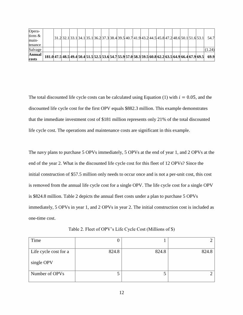
31.2 32.1 33.1 34.1 35.1 36.2 37.3 38.4 39.5 40.7 41.9 43.2 44.5 45.8 47.2 48.6 50.1 51.6 53.1 54.7

Salvage (1.24)

Annual

costs 181.0 47.5 48.5 49.4 50.4 51.5 52.5 53.6 54.7 55.9 57.0 58.3 59.5 60.8 62.2 63.5 64.9 66.4 67.9 69.5 69.9

The total discounted life cycle costs can be calculated using Equation (1) with 𝑖 = 0.05, and the

discounted life cycle cost for the first OPV equals $882.3 million. This example demonstrates

that the immediate investment cost of $181 million represents only 21% of the total discounted

life cycle cost. The operations and maintenance costs are significant in this example.

The navy plans to purchase 5 OPVs immediately, 5 OPVs at the end of year 1, and 2 OPVs at the

end of the year 2. What is the discounted life cycle cost for this fleet of 12 OPVs? Since the

initial construction of $57.5 million only needs to occur once and is not a per-unit cost, this cost

is removed from the annual life cycle cost for a single OPV. The life cycle cost for a single OPV

is $824.8 million. Table 2 depicts the annual fleet costs under a plan to purchase 5 OPVs

immediately, 5 OPVs in year 1, and 2 OPVs in year 2. The initial construction cost is included as

one-time cost.

Table 2. Fleet of OPV’s Life Cycle Cost (Millions of $)

Time 0 1 2

Life cycle cost for a

single OPV

824.8 824.8 824.8

Number of OPVs 5 5 2

13

Initial construction 57.5

Life cycle cost for

fleet of OPVs

4,181.3 4,123.8 1,649.5

The final row of Table 2 is not the budget cost for the navy because the cash flow for the fleet

extends out to year 22 as the final set of OPVs are purchased in year 2. The final row represents

the discounted life cycle costs for the number of OPVs purchases in that year. Those costs should

be discounted again back to the initial year for the OPVs purchased in years 1 and 2. The total

discounted fleet cost can be calculated using Equation (1) where Ct now represents the life cycle

cost for the fleet of OPVs. With a discount rate 𝑖 = 0.05, the total discounted fleet cost is $9.605

billion.

This section has shown how life cycle costs that occur in different years can be combined with

concepts from time value of money to calculate the total discounted life cycle cost of a product.

Since operations and maintenance costs may frequently be a substantial portion of a product’s

total life cycle cost, companies and government agencies need to considering the full life cycle

cost when choosing among multiple product designs. The navy example of purchasing the OPVs

illustrates how the life cycle costs can be calculated based on different cost categories (e.g.,

acquisition, construction, labor, operations and maintenance) and how the life cycle cost for a

single item can be extended to total life cycle costs for multiple items purchased over multiple

years. The next section continues discussing how to use life cycle costs to compare among

multiple alternatives but explains the concepts in terms of computing costs for electric energy.

14

Section 3. Application to Electric Energy Costing with Environmental Considerations

The levelized cost of electricity (LCOE) illustrates how life cycle costing can be used to compare

different technologies for electricity generation on an economic basis. Power plant investment

decisions are typically made by private investors with consideration of many factors including

the competitive wholesale market environment, potential future regulations and incentives, and

the availability of transmission resources over the several-decade life of a plant. Detailed

simulations may be performed to estimate utilization and the resulting revenue the plant may

earn from producing energy or providing spare capacity under changing demand and fuel cost

conditions. The LCOE is generally not used directly for investment decision-making. Instead, it

is a single number that can help explain why one type of investment may be chosen over another

and why the mix of generation resources evolves in response to macroeconomic or regulatory

changes.

3.1 Levelized Cost of Electricity Concepts

The LCOE of a power plant “represents the average [amount of] revenue per unit of electricity

generated that would be required to recover the costs of building and operating [the] plant during

an assumed financial life and duty cycle” [1, p. 1]. On the cost side, the time value of money,

inflation, depreciation, tax impacts, and financing expenses are all taken into account. On the

revenue side, the energy produced in a given time period is estimated by multiplying the plant’s

capacity by its predicted utilization, called its capacity factor. The LCOE computation involves

estimating or assuming values for the following parameters:

15

- Capacity of the plant (MW), the maximum amount of power the plant is capable of

generating;

- Capacity factor (%), the average utilization of the plant;

- Fuel cost ($/MMBtu), the cost per energy unit of the fuel required (if any);

- Heat rate (Btu/KWh), the efficiency expressed in terms of energy units of fuel required to

produce a unit of electric energy (not required for technologies such as wind, solar or

hydro);

- Fixed operation and maintenance (O&M) cost ($/kW-year), representing the costs for

running the plant that do not depend on its utilization;

- Variable O&M cost ($/MWh), additional operating costs per unit of energy generated.

Note that calculations must account for unit conversions with care.

Other than the plant capacity, any of the parameters associated with the plant or its fuel could

vary over the life of the plant. For example, the estimates could account for forecasts of

changing fuel costs, general inflationary pressures on other operating costs, or increasing heat

rate as the equipment ages. A cash flow, tC , representing total operating cost in each year of the

plant’s life ( 1, ,t T ) is then computed and assumed to occur at the end of year t. Note that any

seasonal variation is hidden in the aggregate annual operating cost.The investment, I , required

to build the plant (including engineering, procurement, and construction) is typically modeled as

a single cash flow at time 0 of the project; i.e., the beginning of the first year of the plant’s life.

Having been collapsed into a single value incurred at a single time point, this combined

investment is often called the “overnight cost” of the plant.

16

3.2 LCOE Formulations

If the impact of taxes can be ignored, the LCOE can be computed by estimating the amount of

energy, tE (MWh), the plant will produce in each year, t , of its life and then solving for COEL in

the formula:

1 11 1

T TCOE t t

t tt t

L E CI

i i

(5)

where i is the discount rate. Here, the present value of the incoming cash flows that result from

operating the plant over its T-year life, given the LCOE value, is equated to the present value of

the outgoing cash flows that result from building and operating it. Equivalently, the LCOE is

given by:

1 11 1

T Tt t

COE t tt t

C EL I

i i

(6)

Note that the units of COEL are $/MWh (or they can be scaled to a more convenient basis such as

cents/KWh), which reflects that the LCOE is a revenue per unit of energy production that allows

the plant to just break even in terms of net present value.

To include the impact of income taxes in the calculation, the allowed depreciation expenses can

be subtracted from revenues, along with tax-deductible interest expenses if all or part of the

investment is financed by debt. In this case, the after-tax cash flows for a given value of L are

used in the net present value calculation instead of the pretax ones as shown above.

For a more detailed comparison of generating technologies, along with environmentally-

motivated tax credits, the levelized cost can be decomposed. To do so, the cost components

17

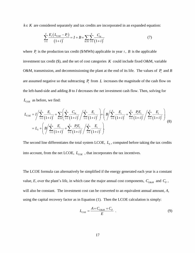
k K are considered separately and tax credits are incorporated in an expanded equation:

1 11 1

T Tt COE t kt

t tt k K t

E L P CI B

i i

(7)

where tP is the production tax credit ($/MWh) applicable in year t , B is the applicable

investment tax credit ($), and the set of cost categories K could include fixed O&M, variable

O&M, transmission, and decommissioning the plant at the end of its life. The values of tP and B

are assumed negative so that subtracting tP from L increases the magnitude of the cash flow on

the left-hand-side and adding B to I decreases the net investment cash flow. Then, solving for

COEL as before, we find:

1 1 1 1 1 1

1 1 1

1 1 1 1 1 1

.1 1 1

T T T T T Tt kt t t t t t

COE t t t t t tt k K t t t t t

T T Tt t t t

S t t tt t t

E C E E PE EL I B

i i i i i i

E PE EL B

i i i

(8)

The second line differentiates the total system LCOE, SL , computed before taking the tax credits

into account, from the net LCOE, COEL , that incorporates the tax incentives.

The LCOE formula can alternatively be simplified if the energy generated each year is a constant

value, E, over the plant’s life, in which case the major annual cost components, &O MC and FC ,

will also be constant. The investment cost can be converted to an equivalent annual amount, A,

using the capital recovery factor as in Equation (1). Then the LCOE calculation is simply:

&O M FCOE

A C CL

E

. (9)

18

3.3 Example LCOE Results

Just as the annual equivalent cost discussed in Section 2.3 allows comparison of alternatives with

different useful lives, the LCOE can be compared across alternative technologies for generating

electricity. For example, in its annual assessment of energy markets over the upcoming decades,

the U.S. Energy Information Administration (EIA) computed the LCOE for new generation

resources included in their forecast through the year 2050 [1]. Table 3 shows the average values

of the LCOE for new resources, weighted by the capacity of each plant projected to be added in

years 2023-2025. Although additional fuel types, such as ultra-supercritical coal, advanced

nuclear, and biomass, have attractive properties, they were not included in the analysis because

EIA did not forecast capacity additions using them to be built in those years.

Table 3. Estimated capacity-weighted LCOE for new generation resources entering service in

2025. Each cost category, as well as the tax credit (NA if unavailable), is levelized separately

and given in 2019 dollars per megawatthour (MWh).

Plant type Capacity factor

(%)

Capital cost

Fixed O&M cost

Variable O&M cost

Trans-mission

cost

Total system LCOE

Tax credit

Total LCOE

including tax credit

Combined cycle 87 7.48 1.59 26.40 1.13 36.61 NA 36.61

Combustion turbine 30 16.10 2.65 46.51 3.44 68.71 NA 68.71

Geothermal 90 20.36 14.50 1.16 1.45 37.47 -2.04 35.44

Wind, onshore 40 23.51 7.51 0.00 3.08 34.10 NA 34.10

Wind, offshore 45 84.00 27.89 0.00 3.15 115.04 NA 115.04

Solar photovoltaic 30 24.12 5.77 0.00 2.91 32.80 -2.41 30.39

Hydroelectric 73 28.89 7.64 1.39 1.62 39.54 NA 39.54

In Table 3, the investment (capital cost) and each category of operating cost, as well as

applicable tax credits, are levelized separately as in Equation (8). Each column (other than

capacity factor) in the table corresponds to an additive term in the equation. The combined

contribution of the applicable tax credits reduces the LCOE as shown.

Levelizing the separate components of LCOE contributes to understanding of the economic

19

characteristics of each technology. For example, the gas-fired combined cycle units and

combustion turbines have relatively low capital cost but higher variable O&M cost, primarily

driven by fuel cost. The renewable resources, especially offshore wind, have high capital cost

but minimal to no variable O&M cost. Renewable resources also have higher fixed O&M costs.

Transmission costs vary according to the distance between the resources and demand centers

and, in competitive wholesale electricity markets, may also depend on the level of congestion in

the lines. The levelized production tax credit (PTC) for geothermal energy and investment tax

credit (ITC) for solar plants are roughly the same magnitude as the levelized transmission costs.

These tax credits can change the ranking of technologies by cost; for example, the PTC makes

the average LCOE of geothermal plants less than that of combined cycle plants and close to that

of onshore wind. The low LCOE for solar photovoltaic plants, even without the ITC, might help

explain why that tax credit is being phased out in the U.S. as of this writing.

Although the LCOE comparison might suggest increased emphasis on renewable resources such

as geothermal, onshore wind and solar photovoltaic, the EIA report cautions that the

dispatchability of resources must also be considered. Fossil-fueled plants continue to be built

partly because system operators can adjust their production levels in response to fluctuations in

the availability of wind, solar, or hydroelectric energy. Geothermal plants are the only

renewable type considered to be dispatchable. The low capacity factors for wind and solar

resources reflect their intermittency, while the low capacity factor for combustion turbines is due

to their primary use as “peaker” units, which are dispatched only in periods of peak demand.

These units continue to be built because of their ability to be started up quickly when needed, but

their high cost limits the proportion of time in which they are operated.

20

3.4. Incremental Costs of Emission Mitigation

Financial incentives, such as tax credits for certain technologies, have been designed to improve

the environmental performance of electricity generation by altering the relative cost profiles of

cleaner technologies. A related approach to environmentally motivated economic assessment is

to estimate the cost of mitigating greenhouse gas (GHG) emissions incrementally. The metric

called levelized cost of conserved carbon (LCCC) is intended to compare alternative options for

reducing carbon emissions. The LCCC quantifies the mitigation cost per unit of avoided

emissions. It relies on estimates of incremental investment, costs, and benefits that would result

from a mitigation measure, as well as the amount by which GHG emissions would be reduced.

Assuming these are constant each year over the life of the mitigation reduction project, let A

be the annualized incremental investment, &O MC be the annual increment in O&M costs, and

B be the annual incremental benefit, all relative to a baseline in which the mitigation measure

is not implemented. The benefits could include reduction in fuel cost, if the measure results in

less fuel use, and would therefore depend on fuel prices. Analogously to Equation (9), the

LCCC is given by [2]:

&O MCCC

A C BL

C

(10)

Note that the units of CCCL are dollars per unit (such as ton of CO2 equivalent) of GHG not

emitted to the atmosphere.

LCCC values can be used to determine abatement cost curves, which are used in climate change

decision making [2]. Thus, broader benefits of carbon mitigation measures, such as improved

health resulting from lowered particulate emissions, are omitted from the analysis to focus on

21

climate change impacts. Moreover, users are cautioned that the LCCC calculation takes into

account only one mitigation option at a time, and cannot account for the interdependence of

impacts among multiple options that could be implemented simultaneously. They may be highly

influenced by energy prices that vary spatially and temporally, and are difficult to predict. The

uncertainty inherent in the LCOE calculation, which involves forecasts of costs over a long time

horizon, is increased in the LCCC because of the need to additionally estimate the baseline as

well as the benefits and the amount of GHG emissions avoided.

Section 4. Concluding Remarks and Future Direction

In this chapter, we reviewed the concepts and perspectives of life cycle costing that are explained

through engineering design of a product as well as planning and management of a project. We

then elaborated on the methodology of life cycle costing, and examined how to calculate the

present value of life cycle costs with and without inflation and annual equivalent cost. Next, we

showed how the basic concept is applied to electric energy costing with environmental

considerations by addressing the levelized cost of electricity and incremental costs of emission

mitigation.

As for the future direction, we would like to point to two noticeable current trends. These are the

changed climate and the continuing series of viruses (e.g., SARS, MERS, and COVID-19). The

changed climate, for example, has caused permafrost melting, resulting in substantial damages to

buildings and infrastructures in numerous countries (see e.g., [3]). In the context of life cycle

costing, should the government policy makers consider such costs in decisions involving fossil

22

fuels (and how)?

For the viruses, for example, the latest news reports a tragic case of gassing tens of thousands of

minks as a SARS-CoV-2 variant jumped from the minks to mink farm workers ( see e.g., [4] ). In

the context of the total cost of ownership, should the life cycle costing of a mink farm take the

costs of addressing infected minks on a massive scale (and their disposal) into relevant decision-

making (and how)? If so, key decisions on whether to build or expand such operations may be

significantly influenced by such costs.

We believe that these trends seem to be unintended consequences of globalism, dependence on

fossil fuel, and industrialization in general. However, by the strict definition of the life cycle

costing that is the total cost of ownership, perhaps in the future, a wide range of broadly defined

classes of design and project problems may be avoided or alleviated as such a perspective will

lead to more circumspective engineering economic decisions.

23

References

1. U. S. Energy Information Administration (2020). Levelized Cost and Levelized Avoided Cost

of New Generation Resources in the Annual Energy Outlook 2020.

https://www.eia.gov/outlooks/aeo/electricity_generation.php (viewed October 23, 2020).

2. Krey, V., O. Masera, G. Blanford, et al. (2014). Annex II: Metrics & Methodology. In:

Climate Change 2014: Mitigation of Climate Change. Contribution of Working Group III to the

Fifth Assessment Report of the Intergovernmental Panel on Climate Change. Cambridge

University Press.

3. Beers, R. (2017). Thawing permafrost causes $51M in damages every year to N.W.T. public

infrastructure: study. CBC News, Nov. 20, 2017.

https://www.cbc.ca/news/canada/north/thawing-permafrost-causes-51m-in-damages-every-year-

to-n-w-t-public-infrastructure-study-1.4408395 (viewed 11 February 2021).

4. Enserink, M. (2020). Coronavirus rips through Dutch mink farms, triggering culls to prevent

human infections. Science, June 9, 2020. doi:10.1126/science.abd2483