Embed Size (px)
Citation preview
SHRP-S-377
Life-Cycle Cost Analysis for Protectionand Rehabilitation of Concrete Bridges
Relative to Reinforcement Corrosion
Ronald L. Purvis, P.E.Khossrow Babaei, P.E.
Wilbur Smith AssociatesBTML Division
Falls Church, Virginia
Kenneth C. Clear
Kenneth C. Clear, Inc.Boston, Virginia
Michael J. Markow, P.E.Cambridge Systematics, Inc.
Cambridge, Massachusetts
Strategic Highway Research ProgramNational Research Council
Washington, DC 1994

SHRP-S-377ISBN 0-309-05755-8Contract C- 104
Product No. 2037, 2038
Program Manager: Don M. HarriottProject Manager: Joseph F. LamondConsultant: John P. Broomfield
Program Area Secretary: Carina S. HreibProduction Editors: Cara J. Tate
February 1994
key words:bridgescorrosion
cost-effectiveness
life cycle
protectionrehabilitationreinforced concrete
Strategic Highway Research ProgramNational Research Council2101 Constitution Avenue N.W.
Washington, DC 20418
(202) 334-3774
The publication of this report does not necessarily indicate approval or endorsement by the National Academy ofSciences, the United States Government, or the American Association of State Highway and TransportationOfficials or its member states of the findings, opinions, conclusions, or recommendations either inferred or
specifically expressed herein.
©1994 National Academy of Sciences
1.5M/NAP_
Acknowledgments
The research described herein was supported by the Strategic Highway ResearchProgram (SHRP). SHRP is a unit of the National Research Council that was authorizedby Section 128 of the Surface Transportation and Uniform Relocation Assistance Act of1987.
This report is a product of the research conducted under SHRP Project C104 by WilburSmith Associates. Ronald L. Purvis of Wilbur Smith Associates was the principalinvestigator for the research. Kenneth C. Clear, Inc., and Cambridge Systematics, Inc.,were subcontractors to the research project.
The methodology to predict the performance of concrete is primarily based on theconcepts developed by Kenneth C. Clear and Siva Venugopalan of Kenneth C. Clear,Inc. Michael J. Markow of Cambridge Systematics, Inc., developed the basic equation ofperformance for concrete, as well as the concepts to determine the user's costs.
The authors wish to thank those who provided many useful comments and suggestionsduring the course of the work reported in this document. They extend special thanks tothe members of the Expert Task Group for SHRP Project C104, members of the SHRPConcrete and Structures Advisory Committee, and Department of Transportation staff inthe states of Minnesota, New York, California, Pennsylvania, and Washington.
in

Foreword
This report consists of three parts. Part One discusses the development of a systematicmethodology to determine the most cost-effective treatment, and its timing, for specificconcrete bridge components that are deteriorating or are subject to deterioration. PartTwo presents the methodology in the form of a handbook for highway agencies. Thehandbook includes nomograms, tables and other aids to facilitate the selection of themost cost-effective strategy. The methodology has also been incorporated into amicrocomputer program. Part Three of this report documents the microcomputerprogram's user's manual, explaining the system's features, options, and displays.
V

Contents
Page
Abstract ................................................... 1
Executive Summary ............................................ 3
Glossary of Variables ........................................... 5
Part I - Methodology
Chapter 1 Overview ......................................... 9
Chapter 2 Technical Goal One: Condition Index Versus Time .............. 13
Chapter 3 Technical Goal Two: Decomposing Condition Index ............. 29
Chapter 4 Technical Goal Three: Cost and Maximum ServiceLife of Treatment ................................... 31
Chapter 5 Technical Goal Four: Condition Index VersusTime After Treatment ................................. 35
Chapter 6 Technical Goal Five: Life-Cycle Cost Analysis ................. 47
Appendix A Flowcharts ....................................... 59
Appendix B Report Format Example ............................... 71
Appendix C Condition Index .................................... 75
Appendix D Time to Deterioration ................................. 79
Appendix E Calculation Two Submodule ............................. 83
vii

Appendix F Criteria for Preventive Maintenance ........................ 89
Part II - Handbook
Chapter 1 Introduction ....................................... 95
Chapter 2 Overview of the Handbook ............................. 97
Chapter 3 Service Life Limitation Due to Functional Features ............... 1.03
Chapter 4 Testing Concrete ................................... 105
Chapter 5 Condition Determination .............................. 113
Chapter 6 Prediction of Performance ............................. 117
Chapter 7 Evaluation of Performance ............................. 131
Chapter 8 Compatible Treatment Alternatives ........................ 143
Chapter 9 Cost Items Associated with Treatment (Agency Costs) ............ 149
Chapter 10 Cost Items Associated with Treatment (User Costs) ............. 155
Chapter 11 Decomposing Concrete Condition Index .................... 161
Chapter 12 Prediction of Performance, Treated Concrete ................. 163
Chapter 13 Optimum Treatment and Time of Treatment .................. 179
Chapter 14 Worked Example .................................. 191
Part III - User Manual for CORRODE
Chapter 1 CORRODE Basics .................................. 211
Chapter 2 Getting Started: The Main Menu ......................... 219
Chapter 3 Bridge Descriptions ................................. 225
Chapter 4 Description of Treatments ............................. 231
Chapter 5 Analyses ........................................ 247
viii

Chapter 6 Viewing Results ................................... 263
Chapter 7 File Management .................................. 269
Appendix A Input Data Defaults and Example Values .................... 271
Appendix B Descriptions of Tests ................................ 283
References .............................................. 289
ix

List of Figures
Part I Page
Figure 1 General Approach ...................................... 10
Figure 2 Bridge Deck Deterioration Model .......................... 15
Figure 3 Condition Index by Predictive Model ........................ 16
Figure 4 Evaluation of Field Structures ............................. 19
Figure 5 Sample Condition Index Curve for a PreviouslyRepaired Structure ..................................... 28
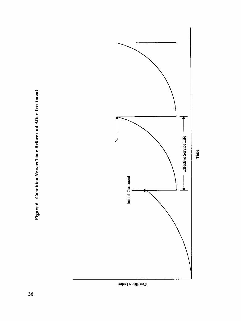
Figure 6 Condition Versus Time Before and After Treatment ............ 36
Figure 7 Corrosion Rate Versus Time .............................. 39
Figure 8 Impacts of Various Treatments on Corrosion Rate .............. 41
Figure 9 Procedure to Estimate Life of Treated Concrete When CorrosionRate is Held Constant ................................... 42
Figure 10 Optimal Timing of Treatment (using concrete overlayas example) ........................................... 53
Figure 11 Comparison of Treatments ............................... 55
Figure 12 Difference of Traffic (using overlay as example) ................ 58
xi

Part H
Figure 4.1 Tests Required ........................................ 106
Figure 5.1 Nomogram to Determine Concrete Condition Index, S .......... 115
Figure 6.1 Nomogram to Determine Age of Concrete at Time toFirst Sign of Deterioration ................................. 119
Figure 6.2 Conceptual Flowchart to Determine ConcretePerformance Equation .................................... 120
Figure 6.3 Nomogram to Determine Parameter B in ConcretePerformance Equation ................................... 122
Figure 6.4 Nomogram to Determine Parameter A in ConcretePerformance Equation .................................. 123
Figure 7.1 Concrete Performance Curves ......................... 132-141
Figure 10.1 Nomogram for User Costs During Treatment .............. 157-158
Figure 10.2 Nomogram to Determine Increment in Travel TimeAcross Bridge ........................................ 159
Figure 10.3 Nomogram to Determine User Costs Prior to Treatment ........ 160
Figure 12.1 Trends of Corrosion Process After Treatment ............. 164-165
Figure 12.2 Nomogram to Determine Effective Service Life ofConcrete After Treatment When Rate of CorrosionContinues at the Same Rate ............................. 166
Figure 12.3 Chart to Find Age of Concrete at Time of First Corrosion ....... 168
Figure 12.4 Nomogram to Determine Effective Service Life of Concrete AfterTreatment When Rate of Corrosion Increases at a Slower Rate ... 169
Figure 12.5 Nomogram to Determine Effective Service Life ofConcrete After Treatment When Rate of CorrosionLevels Off ........................................... 170
xii

Figure 12.6 Nomogram to Determine Effective Service Life of ConcreteAfter Treatment When Rate of Corrosion Decreases ........... 172
Figure 12.7 Trend of Corrosion Process After Treatment ................. 174(Concrete Repaired, Rehabilitated, and/or Protected Previously)
Figure 13.1 Worksheet for Life-Cycle Cost ......................... 181-182
Figure 13.2 Example of Tabulated Treatment Strategy (Treat at tv) ......... 183
Figure 13.3 Example of Tabulated Treatment Strategy (Treat a t_) .......... 184
Figure 13.4 Example of Tabulated Treatment Strategy (Treat between t_ and t_) 185
Figure 13.5 Discount Factors ...................................... 189
Figure 14.1 Worked Example of Tabulated Treatment Strategy (Treat at h,) • • • 208
Figure 14.2 Worked Example of Tabulated Treatment Strategy (Treat at _) . . . 209
Figure 14.3 Worked Example of Tabulated Treatment Strategy(Treat between tp and t_) ................................ 210
Part HI
Figure 1 Main Menu Options ................................... 221
Figure 2 Bridge Menu Options .................................. 226
Figure 3 Treatment Menu Options ............................... 234
Figure 4 Analysis Menu Options ................................. 248
Figure 5 Additional Forms for Input of Corrosion Date ................ 251
Figure 6 Remaining Corrosion Data .............................. 256
Figure 7 Viewing Results ....................................... 264
.,°
Xlll

List of Tables
Part I Page
Table 1 Comparison of Evaluation Schemes ......................... 21
Table 2 Input Data for Example Treatments ......................... 52
Part II
Table 4.1 Number of Tests and Samples ............................ 108
Table 6.1 Correlation of Rate of Deterioration and Resistivity ............ 127
Table 6.2 Estimates of Surface-LevelChloride Content in 10 Years ........ 127
Table 8.1 Selection of Compatible Deck Treatment Alternatives .......... 147
Table 8.2 Selection of Compatible Structural Treatment Alternatives ....... 148
Part 11I
Table 4.1 Selection of Compatible Deck Treatment Alternatives .......... 232
Table 4.2 Selection of Compatible Structural Treatment Alternatives ....... 233
Table 5.3 Number of Tests and Samples ............................ 252
xv

List of Flowcharts
Part I, Appendix A Page
Flowchart 1 General Technical Methodology for Technical Goal One ....... 60
Flowchart 2 General Information Module ........................ 61
Flowchart 3 Protect Information Module ......................... 62
Flowchart 4 Present Information Module ......................... 63
Flowchart 5 Time-To Module ................................ 64
Flowchart 6 Post-Deterioration Submodule ........................ 65
Flowchart 7 Calculation One Submodule ......................... 66
Flowchart 8 Pre-Deterioration Submodule ........................ 67
Flowchart 9 Calculation Two Submodule ......................... 69
Flowchart 10 Repair Information Module ......................... 70
xvii
Abstract
A systematic methodology is presented for highway agencies to use at the project level todetermine the most cost-effective treatment, and its timing, for specific concrete bridgecomponents that are deteriorating or are subject to deterioration. The methodology isset forth in the form of both a handbook and a computer program. The methodology inits present form applies only when the predominant concrete deterioration is associatedwith chloride-induced corrosion of the reinforcing steel. The methodology is designed tobe flexible and can be tailored to suit the needs of individual highway agencies.

Executive Summary
The deterioration of concrete bridges is a major problem in the operation of the nation'shighway system. The cost of repairing or replacing deteriorating bridges is one of themost expensive items faced by highway agencies, and it is increasing rapidly. The maincause of the deterioration is the use of salt in winter maintenance operations. The saltpenetrates the concrete and corrodes the reinforcing steel, eventually resulting in internalcracking and surface spalling of the concrete. The deterioration occurs on all concretebridge components, including decks, superstructure elements, and substructure elements.Similar corrosion-induced deterioration also occurs on concrete components exposed tomarine environments.
In order to reduce the cost of bridge maintenance at the network level, it is essential thatrational actions are taken at the project level. This report provides a systematicmethodology to guide technical personnel of highway agencies to rational decisionsregarding treatment of specific concrete bridge components. The methodology appliesthe concept of life-cycle cost. The output from the methodology answers the user'squestions regarding the type and timing of treatment to achieve the lowest life-cyclecost. The methodology is set forth in the form of both a handbook and a computerprogram.
The methodology takes the following factors into account to conduct life-cycle costanalysis:
1- The condition of the concrete component and itsperformance.
2- The technical compatibility, cost, and service life of the rangeof treatment alternatives from which the selection can bemade.
The methodology recommends which site-specific condition data to obtain and how touse the data to quantify the concrete condition in terms of an index. The methodologyalso provides the user with the performance curve predicting the condition index of thecomponent in the future, based on the available condition data. From the performance
curve, the user will determine the time to maximum tolerable condition index. The timeof maximum tolerable condition is not necessarily the optimum time to treat theconcrete. The rest of the methodology is used to determine the type of treatment and itstiming to achieve the lowest life-cycle cost.
The methodology presents a range of potential alternatives to treat the concrete andhelps the user screen out the alternatives that are not technically compatible with thecomponent. The methodology then shows the user how to estimate costs involved inapplying each appropriate type of treatment. Both agency and user costs can beincluded.
Since the methodology applies the life-cycle cost concept, the performance of concreteafter the treatment also needs to be predicted. The methodology utilizes the concept of"trend in the rate of corrosion after the treatment" to predict the performance after thetreatment. Each potential treatment alternative is represented by a certain trend in therate of corrosion of reinforcing steel after the treatment. The user, however, has theoption of changing the trend in the rate of corrosion that is assigned to a giventreatment, based on the agency's experience with that particular treatment. Unlike thetrend in the rate of corrosion, the actual rate of corrosion value generally does not play arole in the methodology and it is only needed when certain concrete conditions arepresent. However, since historical rate of corrosion data are limited at this time, theavailability of further rate of corrosion data can support the rate of corrosion trendsassigned to various treatments in the methodology. Therefore, agencies are encouragedto collect pre- and post-treatment rate of corrosion data from selected sites.
To conduct life-cycle cost analysis, the user of the methodology will first select a type oftreatment from the range of compatible treatment alternatives available. The user willthen consider treating the concrete component at different points in time for life-cyclecost comparison. Those different points in time are bounded by (1) the present time, (2)the time of maximum tolerable condition. The economic analysis of each of thestrategies considered is done systematically. All costs associated with each strategy,including costs of repeated cycles of treatment (agency and user costs) are then inputinto the system. The output from the system is the life-cycle cost of each strategy. Thelowest life-cycle cost represents the optimum strategy (i.e., optimum time of treatment)for the type of treatment selected.
Once the optimum time of treatment and life-cycle cost for one treatment is determined,the user will employ the same procedure to determine the optimum time of treatmentand life-cycle cost for other treatments. At the end, the user will be able to prioritizethe various types of treatments based on their life-cycle costs. The most cost-effectivetreatment will be the one with the lowest life-cycle cost, and it should be applied at itsoptimum time.
4
Glossary of Variables
a Percent of free-flow travel time across bridge, representingincrement in travel time when deck condition is maximumtolerable.
A Constant controlling rate of deterioration in concreteperformance equation.
B Constant controlling rate of deterioration in concreteperformance equation.
C Two-way capacity of bridge during normal periods, vehiclesper day.
C1 Two-way capacity of bridge during construction, vehicles perday.
CL Percent of concrete samples with bar-level chlorides higherthan corrosion threshold value.
C. Number of cement sacks per cubic yard of concrete.
Cm Rate of corrosion of reinforcing steel when concrete conditionis maximum tolerable.
Cp Rate of corrosion of reinforcing steel measured at present,corresponding to 90th percentile value (average rate ofcorrosion plus 1.282 standard deviation).
Cr Rate of corrosion of reinforcing steel at previous repair,rehabilitation, and/or protection.
C* Rate of corrosion of reinforcing steel at the time of plannedtreatment.
5

COST Cost of last cycle of treatment in plarming horizon.
d Depth of bar cover corresponding to 10th percentile value(average depth minus 1.282 standard deviation).
d. The present worth factor.
D Total deck area, square feet.
DELAM Percent of concrete area that is delan_nated (not includingspalls).
DF Discount factor.
DF20 Discount factor corresponding to Year 20 in planning horizon.
EI Effective interest rate.
ESL Effective service life of treated concrete.
J The total discounted life-cycle cost to be minimized for a given treatmentstrategy.
K The ratio of the slope of corrosion rate line after treatment tothe slope of corrosion rate line before treatment.
Ko Chloride concentration of water, parts per million.
Kt Value of bridge user time while traveling, dollars per minuteper vehicle.
K2 A calibrating constant for user cost prior to treatment, dollarsper vehicle.
1 The life of each treatment following the initial treatment.
m Periodic maintenance cost, only cathodic protection.
M A fixed time as for mobilization.
n Number of each consecutive year in planning horizon.
n. An exponent controlling the growth of user cost with deteriorating deckcondition.
6

N A constant representing the ratio of delaminated concreteareas to spalled concrete areas in a typical case.
P Concrete water-cement ratio.
Pr Productivity of treatment, square feet per day.
qo Average two-way daily traffic volume across the bridge,vehicles per day.
r Discount factor for optimization procedure.
Rt Age of concrete at time to first sign of corrosion-induced deterioration(original version of ta).
RS Remaining effective service life of treated concrete beyondthe planning horizon.
S Concrete condition index.
Si Depth of steel below concrete surface.
Sm Maximum tolerable concrete condition index.
Sp Concrete condition index at present.
Sr Concrete condition index at time of previous repair,rehabilitation, and/or protection.
St Concrete condition index predicted for concrete age of t.
$45 Concrete condition index of 45.
S(t*) Percent of deck area that is distressed at the time of treatment.
SLVG Salvage value, present worth.
SPALL Percent of concrete area that is spalled.
t Time since initial construction of concrete (age of concrete),years.
t, Duration of concrete treatment, days.
7

ta Age of concrete at time to first signs of corrosion-induceddeterioration, years.
t_ Free-flow travel time across the bridge, minutes.
t_ Age of concrete at the time of maximum tolerable concretecondition, years.
to Age of concrete at time to first sign of corrosion, years.
ta, Age of concrete at present time, years.
t_ Age of concrete at the time of previous repair, rehabilitation,and/or protection.
tt Increment in travel time across the bridge (or detour aroundthe bridge) caused by construction, minutes.
t" Age of concrete at the time of planned treatment, years.
t45 Age of concrete at the time of condition index of 45, years.
U Incremental increase in user cost due to worsening deck condition, dollarsper vehcile.
U1 User cost during the treatment period, donars.
U2 User cost due to worsening deck condition, dollars per year.
Wm Mixing water in percent of concrete volume.
Zt Concrete surface chloride content corresponding to 90thpercentile value (average chloride content plus 1.282 standarddeviation), percent of concrete weight.
Za Concrete surface chloride content at time to deterioration, percent ofconcrete weight.
ot A constant used in congestion cost formula.
/3 An exponent used in congestion cost formula.

PART I--METHODOLOGY
1. Overview
The deterioration of concrete bridges is a major problem in the operation of the nation'shighway system. The cost of repairing or replacing deteriorating bridges is one of themost expensive items faced by highway agencies, and it is increasing rapidly. The maincause of the deterioration is the use of salt in winter maintenance operations. The saltpenetrates the concrete and corrodes the reinforcing steel, eventually resulting in internalcracking and surface spalling of the concrete. The deterioration occurs on all concretebridge components, including decks, superstructure elements, and substructure elements.Similar corrosion-induced deterioration also occurs on concrete components exposed tomarine environments.
In order to reduce the cost of bridge maintenance at the network level, rational actionsare required at the project level on the basis of life-cycle costs. This report discusses amethodology that provides systematic procedures to allow valid life-cycle cost comparisonof the available options for protecting and rehabilitating specific concrete bridgecomponents. These procedures are set forth in the form of both a handbook and acomputer program. The handbook is contained in Part II of this document; thecomputer program user's manual, in Part III.
Figure 1 summarizes the general approach of the methodology. Generally, themethodology involves the following objectives:
• Obtain general information on the component, and determine thepresent condition of the component.
• Quantify concrete condition in terms of an index.
• Predict future condition index.
• Estimate cost of treatment, and determine treatment's maximum possible servicelife on the basis of non-corrosion-related distress.
9

lo
• Predict concrete condition index after treatment.
• Conduct life-cycle cost analysis to determine the optimum treatmentand its timing.
To accomplish those objectives, the methodology is aimed at the following technicalgoals.
1.1 Technical Goal One: Condition Index Versus Time
Technical Goal One quantifies the present condition of the concrete in terms of anindex. Also, it predicts the condition index at any time in the future. To do so, itsupplies two appropriate data points on the plot of condition index versus time, so thatthe concrete performance curve can be determined prior to any treatment. Theperformance curve is determined for all possible cases (i.e., for concrete members whichwere built with and without protective systems at the time of the initial construction; forpreviously rehabilitated members as well as members which have never beenrehabilitated; for members presently showing physical distress; and for members whichare not yet salt contaminated or distressed).
1.2 Technical Goal Two: Decomposing Condition Index
Technical Goal Two involves devising a means of decomposing the predicted concretecondition index into its distress component parts for the purpose of estimating thephysical distress in the concrete in the future, so that treatment cost estimates can beperformed.
1.3 Technical Goal Three: Cost and Maximum Service Life of Treatment
Technical Goal Three provides cost and service life information (maximum possible lifebased on non-corrosion-related distress) for alternative procedures for treatment ofconcrete.
1.4 Technical Goal Four: Condition Index Versus Time after Treatment
Technical Goal Four supplies procedures to predict the condition index with time aftereach applicable treatment.
11

1.5 Technical Goal Five: Life-Cycle Cost Analysis
Technical Goal Five provides procedures to determine the treatment that results in thelowest life-cycle cost, as well as the optimum time to apply that treatment.
1.6 Report Format
This report discusses the technical goals of the methodology. Flowcharts of variousmodules, questions to the user, and decisions are included in Appendix A. They arehelpful in understanding the discussion. Although the technical basis and details arevoluminous, the user will see only a short series of questions and then the findings. Asample computer run is demonstrated for Technical Goal One, Condition Index VersusTime, in Appendix B. This computer run is not related to the CORRODE systemdescribed in Part III of this document.
12

2. Technical Goal One
Condition Index Versus Time
2.1 Condition Index
The first step is to quantify the concrete condition. Current research on this and otherSHRP research projects suggests that three quantities are indicators of current concretecondition as affected by corrosion:
1. Percent of bar-level concrete samples with chloride content higher thanthe corrosion threshold value (CL).
2. Percent of concrete area that is delaminated (DELAM), not includingspalls.
3. Percent of concrete area that is spalled (SPALL).
Of these, when considering treatment options at a given time, spalling is the mostimportant factor, delamination is second in importance, and chloride contamination atthe level of reinforcing steel is the third most important. For the purposes of thisproject, the relative importance of each of these three factors (as an indicator of theneed of treatment) is expressed by assigning the following weights:
Spalling is three times more important than delamination, while delaminationis 2.5 times more important than bar-level chloride contamination.
The condition index (S) may then be quantified at the time of condition survey and onthe basis of condition data as follows:
S = [CL + 2.5 (DELAM) + 7.5 (SPALL)] / 8.5 (Eq. 2.1)
Appendix C shows in detail how the condition index is calculated. As the concretegradually deteriorates, its condition index increases. The condition index has a
13
mathematical maximum of 100 and a minimum of 0, although practically speaking, it isbelieved that the condition index should not be allowed to exceed 45.
2.2 Prediction of Future Condition Index
Corrosion-induced deterioration in concrete is typically represented in the literature as apiecewise linear function, as shown in Figure 2a. This curve itself is an approximation ofhow deterioration actually progresses in the field. However, the three linear segments(i.e., the regime of zero damage prior to corrosion initiation at to; the intervening periodup to the time to deterioration at to; and the growth of damage thereafter) cannotconveniently be represented by a single equation. The deterioration model (ConditionIndex) assumed in this study is therefore shown in Figure 2b. This S-shaped, or logistic,curve is a plot of the following equation.
St = 100 / [1 + A exp(-Bt)] (Eq. 2.2)
where
St = concrete condition index predicted for concrete age of t
A,B = parameters controlling the rate of deterioration and the shapeof the curve
t = time since initial construction (age of concrete), years
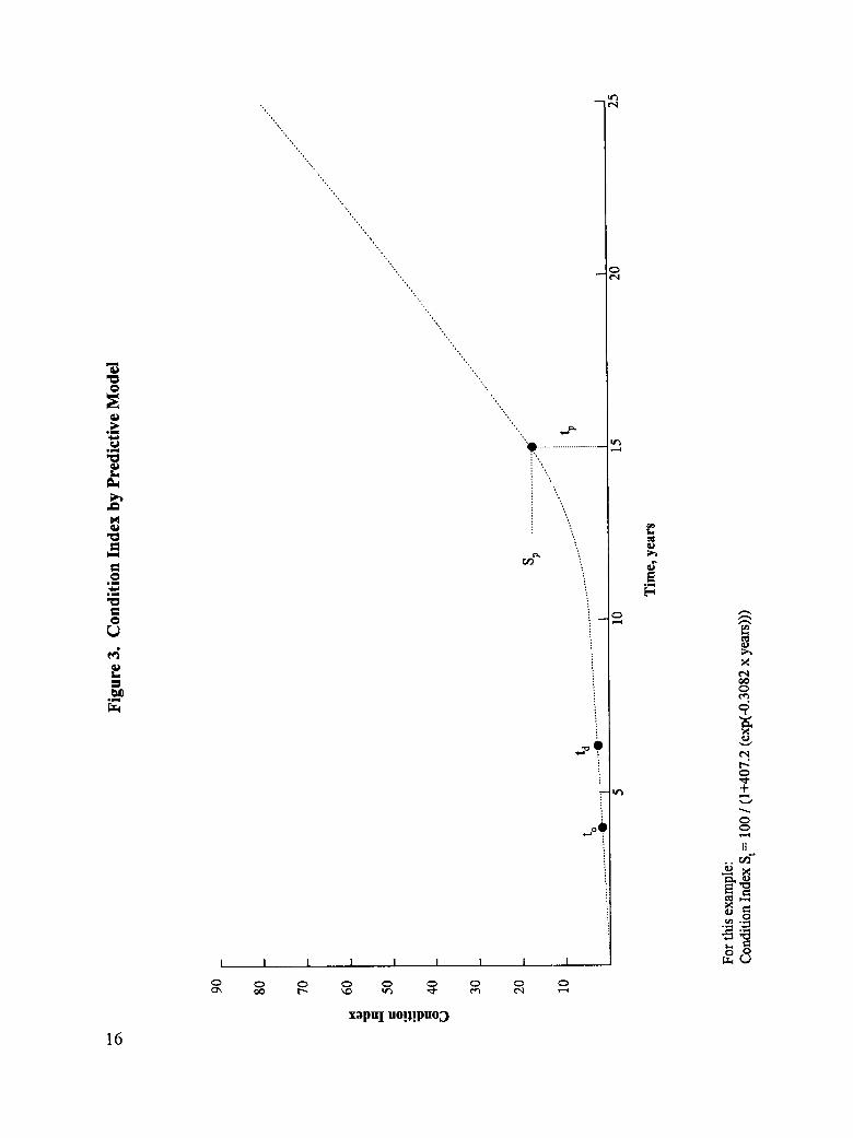
An example of the condition index versus time curve is shown in Figure 3. The twounknown parameters of A and B in the equation are found based on the site-specificdata. To find the parameters, two appropriate data points are required. Each data pointrepresents the condition index and the corresponding concrete age. Because of thewidely varying members, and their past, present, and future conditions, the two neededdata points on the condition index versus time curve cannot always be at the samecondition or age. When possible, one of the points will be the age of concrete at theinitiation of deterioration (t,) with an assigned condition index (S0), and the other will bethe age of concrete at the present (tp) with the condition index at the present (Sp).
As discussed previously, the two terms representing the age of concrete at the initiationof corrosion and the start of physical distress are to and td, respectively. For the purposesof this effort, the following condition indices were assigned to those items on the basis ofexperience:
1. Condition index at to (S_.;."10 percent chloride contamination, 0percent delamination, and 0 percent spalling. Therefore, So = 1.2.
14
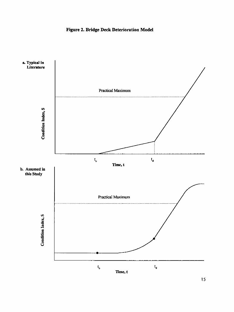
Figure 2. Bridge Deck Deterioration Model
a. Typical inLiterature
0
Q
to tdTime, t
b. Assumed inthis Study
Practical Maxim
,$..m
O
to tdTime, t
15
",
"0
P_, i ',
e4 xL.. t'N
a_
&
II
Nx
o
I I I 1 1 I I I I
xop_ uo!_!puo_)
16
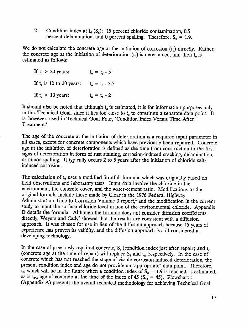
2. Condition index at t_ (Sa): 15 percent chloride contamination, 0.5percent delamination, and 0 percent spalling. Therefore, Sd = 1.9.
We do not calculate the concrete age at the initiation of corrosion (to) directly. Rather,the concrete age at the initiation of deterioration (td) is determined, and then to isestimated as follows:
If td > 20 years: to = td" 5
If tdis 10 to 20 years: to = td - 3.5
If td < 10 years: to = td- 2
It should also be noted that although to is estimated, it is for information purposes onlyin this Technical Goal, since it lies too close to td to constitute a separate data point. Itis, however, used in Technical Goal Four, "Condition Index Versus Time AfterTreatment."
The age of the concrete at the initiation of deterioration is a required input parameter inall cases, except for concrete components which have previously been repaired. Concreteage at the initiation of deterioration is defined as the time from construction to the firstsigns of deterioration in form of rust staining, corrosion-induced cracking, delamination,or minor spalling. It typically occurs 2 to 5 years after the initiation of chloride salt-induced corrosion.
The calculation of ta uses a modified Stratfull formula, which was originally based onfield observations and laboratory tests. Input data involve the chloride in theenvironment, the concrete cover, and the water-cement ratio. Modifications to theoriginal formula include those made by Clear in the 1976 Federal HighwayAdministration Time to Corrosion Volume 3 report, I and the modification in the currentstudy to input the surface chloride level in lieu of the environmental chloride. AppendixD details the formula. Although the formula does not consider diffusion coefficientsdirectly, Weyers and Cady2 showed that the results are consistent with a diffusionapproach. It was chosen for use in lieu of the diffusion approach because 15 years ofexperience has proven its validity, and the diffusion approach is still considered adeveloping technology.
In the case of previously repaired concrete, Sr (condition index just after repair) and tr(concrete age at the time of repair) will replace Sdand td,respectively. In the case ofconcrete which has not reached the stage of visible corrosion-induced deterioration, thepresent condition index and age do not provide an "appropriate" data point. Therefore,ta, which will be in the future when a condition index of Sd = 1.9 is reached, is estimated,as is t45,age of concrete at the time of the index of 45 ($45 = 45). Flowchart 1(Appendix A) presents the overall technical methodology for achieving Technical Goal
17
One. It shows various modules and decision point.,;involved in a methodology applicableto various concrete members and state of distress. The specifics of each module arepresented below.
General Information Module (Flowchart 2)
Certain data are required in all instances. These data will be obtained in the GeneralInformation Module as responses to questions, including the following:
Year Constructed? Give the year the concrete was constructed.
Size of Member in Square Feet? For a deck give the top surface area. For othermembers, give the overall surface area being analyzed.
Type of Member? Deck or Substructure? If a deck is specified, the question is asked:Does the deck have an asphaltic concrete overlay? If the answer is "YES," such is notedin the output so a cost may be assigned to removal of the overlay during treatment.
Has the member previously been repaired? Answer "YES" or "NO." If the answer to thequestion above is "YES," proceed to the Repair Information Module, and then go to thePresent Information Module. If the answer is "NO," proceed to the Protect Information,Present Information, and Time-To Modules.
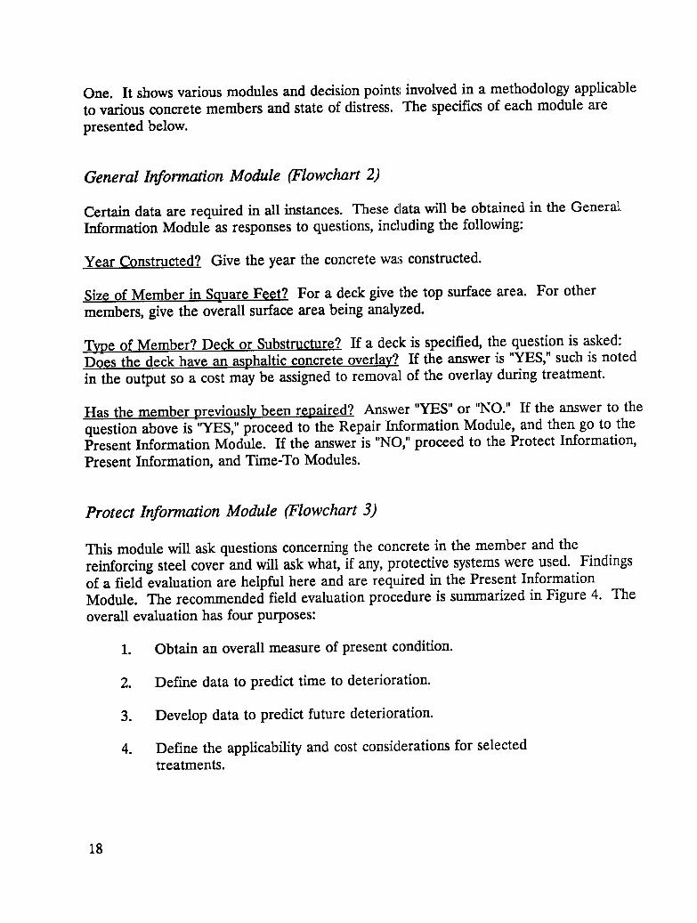
Protect Information Module (Flowchart 3)
This module will ask questions concerning the concrete in the member and thereinforcing steel cover and will ask what, if any, protective systems were used. Findingsof a field evaluation are helpful here and are required in the Present InformationModule. The recommended field evaluation procedure is summarized in Figure 4. Theoverall evaluation has four purposes:
1. Obtain an overall measure of present condition.
2. Define data to predict time to deterioration.
3. Develop data to predict future deterioration.
4. Define the applicability and cost considerations for selectedtreatments.
18
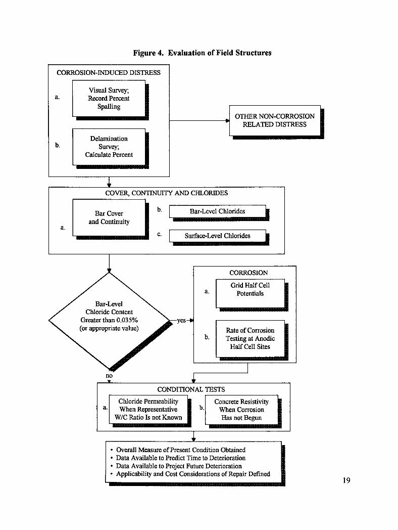
Figure 4. Evaluation of Field Structures
CORROSION-INDUCED DISTRESS
Visual Survey;a. RecordPercent
SpaUing j OTHERNON-CORROSIONRELATEDDISTRESS
Delaminationb. Survey;
CalculatePercent
F
COVER, CONTINUITYAND CHLORIDES
Bar Cover _ b. Bar-Level Chloridesand Continuity |
a.
c. Surface-Level Chlorides
CORROSION
Grid Half Cell _!
a._roll
yes_ _"
Rate of Corrosion /
b. Testing at Anodic l[
Half Cell Sites I
no _CONDITIONAL TESTS
1C on e o o iliICon rete e ia. When Representative _ b. When Corrosion
W/C Ratio Is not Known I Has not Begun I
/
• Overall Measure of Present Condition Obtained
!• Data Available to Predict Time to Deterioration
• Data Available to Project Future Deterioration• Applicability and Cost Considerations of Repair Defined
19

As a result, the evaluation varies somewhat from that defined in SHRP research by Cadyand Gannon. 3 However, this variance is not a conflict, in that the SHRP conditionevaluation manual only involves the first item above (i.e., measure present condition).Table 1 compares the evaluation schemes of this research project and of the SHRPcondition evaluation manual and notes the reasons for the differences.
Returning to the questions asked in this module:
Question 1: What is the water-cement ratio of the concrete surrounding the reinforcingsteel? An answer in the range of 0.2 to 0.7 is required. The ratio may be obtained fromproject records or by other means. This information will be used to calculate t,(concrete age at the time of first sign of deterioration) on members which have not beenpreviously repaired if td is not otherwise known.
Question 2: Is data on the actual reinforcing steel cover available? If the answer is"NO," the user is asked to input the design cover in inches and the 10th percentile covervalue is calculated as the design cover minus 0.48 inches (1.2 centimeters) (a standarddeviation of 0.38 inches (0.97 centimeters) is assumed). Of course, the result must begreater than 0. If the answer is "YES," The user is asked to input the cover data and theaverage, standard deviation, and 10th percentile cover value (average cover - 1.282 *standard deviation) is calculated. The recommended minimum number of covermeasurements is 40 per member or per 5,000 square feet (465 square meters), whicheverresults in the larger number of measurements.
Question 3" Was the concrete constructed with a corrosion protective system listedbelow, or was one added before the surface-level chloride exceeded the critical valuewhich would later diffuse and cause bar corrosion? (the critical surface chloride valuemay be obtained using the procedure outlined in Appendix F.) If the answer is "NO," weproceed to the Present Information Module. If the answer is "YES," The following list ofpossible protective systems is provided, and the user is requested to designate thosewhich are included and to define the years of additional service (i.e., years of additionaltime to deterioration) which result from each protective system. Note that these years ofservice are in addition to that provided by the concrete itself which is affected by water-cement ratio and cover depth.
1. Epoxy-Coated Reinforcing Steel2. Latex-Modified Concrete overlay3. Concrete Overlay (including low-slump dense concrete)4. Silica Fume Concrete, Full Depth5. Silica Fume Concrete, Overlay6. Waterproof Membrane with Asphalt Concrete Overlay7. Penetrating Sealer
20

Table 1. Comparison of Evaluation Schemes
SHRP Condition Evaluation Manual3 This Project
1. Concrete Permeability 1. Concrete permeability (and resistivity)
Determining the relative permeability of concrete AASHTO T277 (and KCC INC Resistivity)in the field as in appendix G of Volume 8 (surface AASHTO T277 is required for permeability whenairflow), representative water-cement ratio of concrete is
needed.
Reasons: Lack of adequate data relating water-cement ratio and permeability by surface airflow.States are more familiar with AASHTO T277 test
method which has a large data base. Resistivity(water saturated, 73 degrees F) is also required,when corrosion deterioration has not begun.
2. Chloride content 2. Chloride content
Recommends procedure applicable to the field. It Procedure given in Reference 3 or AASHTOis given in Appendix F of Volume 8. T260-84 procedure for total chloride.
3. Recommended number of samples 3. Recommended number of samples
None, except for cover (40 per member regardless A specific number of tests and/or samples areof size), recommended for all variables used in predicting
time-to-deterioration. Both "per member" and"per 5000 square feet." requirements.
4. Chloride measurements and/or profiles 4. Chloride measurements and/or profiles
Recommended only when 10 percent or less of Chlorideprof'de data (specifically surface chloridehalf cell potentials are more negative than -0.20 and bar level chloride) are required irrespective ofvolt CSE. the hal cell potential values.
5. Corrosion rate 5. Corrosion rate
Recommended only when 90 percent or more of Required when the chloride content at the barthe half cell potentials are more negative than depth is greater than chloride threshold (0.035-0.20 volt CSE. percent) and the concrete was repaired/
rehabilitated previously.
6. Half cell potentials 6. Half cell potentials
Survey done at all times. Potential surveys are used only to identify the mostanodic areas to locate points for corrosion ratemeasurements when bar-level chloride is greaterthan chloride threshold (0.035 percent).
21
8. Surface Protective Coating9. Concrete with Corrosion Inhibitor Admixture10. Cathodic ProtectionI1. Other
Thus, for each protective system designated, the question is asked: How many years willthe first signs of deterioration be delayed by the designated protective system? Ananswer is required, but the effect of the conventional concrete (as defined by its water-cement ratio and the reinforcing steel cover) must .not be included in the answer. Theanswer will be added to td from the Pre-Deterioration Submodule, if that module is used.
When a corrosion inhibitor admixture is used as the protective system, an additionalquestion is asked: How much inhibitor is used in the concrete? The Present Modulewill use the answer to adjust the chloride threshold used in determining the presentcondition index (Sp) (e.g., 0.035 percent of concrete weight).
For concrete overlays (low-slump dense, latex-modified, and silica fume), the water-cement ratio for input into the t0 formula must be adjusted to reflect the average water-cement ratio of the concrete cover (i.e., part may be overlay and part may be baseconcrete). To accomplish this, the following questions are asked:
What is the thickness of the overlay?
What is the overlay representative water-cement ratio?
The water-cement ratio of the concrete surrounding the reinforcing steel and theconcrete cover is already known. A "prorated average water-cement ratio" will bedefined and input (in lieu of the answer to Question 1) into the to formula. As anexample, if the total cover (per this project's method) is 2.75 inches (7.0 centimeters), theoverlay is 2.0 inches (5.1 centimeters), the representative water-cement ratio of theoverlay is 0.38, and the water-cement ratio of the base concrete is 0.45, then the inputwater-cement ratio will be:
[(0.38 * 2.0) + (0.45 * 0.75)] / (2.75) = 0.40
If more than one protective system is designated (such as epoxy-coated bar and a latex-modified concrete overlay), the years of additional life for each will be added to t0.
22

Present Information Module (Flowchart 4)
The Present Information Module is next; it defines the present condition (states ofdistress). The module first asks for information regarding the age of the member beingexamined. The following questions are then asked, data entered, and the answers usedto calculate the present condition index, Sp.
Question 1: What square footage of the area is spalled (to determine SPALL)?
Question 2" What square footage of the area is delaminated (to determine DELAM)?Do not include spalls.
Question 3" What percentage of concrete samples at reinforcing steel level have chloridecontent higher than the corrosion threshold (CL)? A minimum of 10 bar level chloridesper member, or per 5,000 square feet (465 square meters) of member surface exposed tosalt environment (whichever is greater), is recommended.
Question 4" Are chloride-bearing aggregates involved which have been shown not tocontribute chlorides to the corrosion process? Answer "NO" or "YES." If the answer is"YES," input the percentage (by weight of concrete) of "benign" chloride locked in theaggregate.
From the answers to Questions 3 and 4, and with corrosion inhibitor information fromthe Protect Information Module, the user calculates the percentage of the bar-levelchloride values which exceed the total of 0.035 percent (by weight of concrete) plus theaggregate benign chloride plus the corrosion inhibitor offset.
Then, the present condition index, Sv will be calculated as [CL + (2.5 * DELAM) +(7.5 * SPALL)] / 8.5, corresponding to the age of the concrete at preset, tp. Thiscompletes the Present Information Module. Then the Time-To Module follows.
7_me-To Module (Flowchart 5)
The results of the Present Information Module calculation of Spare checked. If Spisgreater than 1.9, it is concluded that h occurred in past, and we proceed to the Post-Deterioration Submodule. If Spis less than 1.2, proceed to the Pre-DeteriorationSubmodule. If Spis between 1.2 and 1.9, tdis defined as equal to tv and another datapoint at some time in the future will be defined via the Calculation Two Submodule.
23
Starting with the Post-Deterioration Submodule:
Post-Deterioration Submodule (Flowchart 6)
The submodule asks for technical "input data" regarding the time to deterioration.
Ouestion 1: From the present data, it has been determined that this member is showingsigns of corrosion-induced deterioration. What year was chloride-induced corrosion firstnoticed? Possible answers are "Year," or "Don't Know." If a year is given, it is accepted(and td = Year Given minus Year Built), no other background data are requested, andthe user proceeds. If the answer is "Don't Know," proceed to the Calculation OneSubmodule, knowing that td must lie between the Year Built and the Present.
Calculation One Submodule (Flowchart 7)
In this submodule the user calculates the "past" td. Input data include that from theGeneral, Protect, and Present Information Modules as follows:
1. Adjustment of ta, if any, because of a protective system installed atthe time of initial construction.
2. Average, standard deviation, and 10th percentile concrete cover.
3. Water-cement ratio of the concrete between the surface and bar.
The module then requests data on the surface chloride level at present to calculate tdforthe concrete. The methodology recommends that at least eight surface chloride levels(from 0.25 inches (0.6 centimeters) to 0.75 inches (1.9 centimeters)) be determined permember or per 5,000 square feet (465 square meters), whichever results in the largernumber. Surface chloride samples must not be taken in patched areas. Upon receipt ofthese data, "t" is calculated as the "Year Data Taken" minus "Year Concrete Built" and tdis calculated from the formula presented in Appendix D and adjusted per the first itemabove.
Pre-Deterioration Submodule (Flowchart 8)
When considered td in the future, the same input items are requested or obtained fromthe other modules as for the Post-Deterioration Submodule. However, if the surfacechloride values axe extremely low because of lack of exposure age, the calculation of tdwill be incorrect. Therefore, the surface chlorides are checked after they are entered. If
24

the average is greater than or equal to 0.10 percent of chloride by weight of concrete,proceed as per the Post-Deterioration and Calculation One Submodules. If the averageis less than 0.10 percent, proceed to the Adjust Submodule as follows.
When the surface chlorides are quite low, the user needs an estimate of surface chloridevalues in 10 years. To aid in this estimate, input the mean annual snowfall in inches inthe vicinity of the structure and then answer the subsequent questions as well.
Is the concrete exposed to a marine environment, YES or NO?
If the answer to the marine environment question is "YES," answer another question: Isthe member within 25 feet (7.6 meters) of the seawater?
Based on the above responses and the following table, the surface chloride level 10 yearsinto the future is estimated. Known data include the question answers, the presentsurface chloride (Zt), and the exposure age to date (t).
Snow Range* Seawater* Surface Clorides(inches) Exposure in 10 years, % Greater of:
0 to 3 No [Z_ * (t+ 10)/t] or 0.04%3 to 12 No [Z_ * (t+10)/t] or 0.10 %0 to 12 Yes > 25 ft [Z_ * (t+10)/t] or 0.10 %0 to 12 Yes < 25 ft [Z_ * (t+10)/t] or 0.25 %>12 No [Z_* (t+10)/t] or 0.25 %>12 Yes > 25 ft [Zt * (t+10)/t] or 0.35 %>12 Yes < 25 ft [Zt * (t+10)/t] or 0.45 %
• One inch is 2.54 centimeters; one foot is 0.305 meters.
Then ta is calculated based on the appropriate Zt from the table above, while "t" in theequation for Z t is equal to "present t" (concrete age at the time of measuring surfacechlorides) plus 10 years.
Calculation Two Submodule (Flowchart 9)
The user then must continue the Pre-Deterioration Submodule to estimate the concrete
condition at some time in the future after t0. This is done using the Calculation TwoSubmodule. This estimate is required to determine the slope of the deterioration versustime curve after corrosion is active. By this time, chloride is present at the reinforcingsteel level in excess, and the corrosion and deterioration rates will be dictated by manyfactors, including the steel concentration, oxygen availability, and the resistivity of theconcrete in the field. All these factors are not known. However, an estimate of whetherthe deterioration rate will be low, medium, or high should be possible, and standardcurves can be assigned to each rate designation. This assignment can be based on the
25
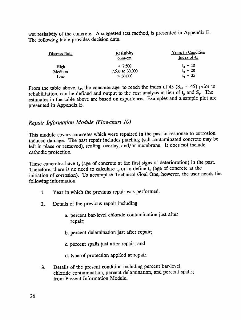
wet resistivity of the concrete. A suggested test method, is presented in Appendix E.The following table provides decision data.
Distress Rate Resistivity Years to Conditionohm-cm Index of 45
High < 7,500 td + 10Medium 7,500 to 30,000 td + 20Low > 30,000 h + 35
From the table above, ta5the concrete age, to reach the index of 45 ($45 = 45) prior torehabilitation, can be defined and output to the cost analysis in lieu of tv and S0. Theestimates in the table above are based on experience. Examples and a sample plot arepresented in Appendix E.
Repair Information Module (Flowchart 10)
This module covers concretes which were repaired in the past in response to corrosioninduced damage. The past repair includes patching (salt contaminated concrete may beleft in place or removed), sealing, overlay, and/or membrane. It does not includecathodic protection.
These concretes have td (age of concrete at the first signs of deterioration) in the past.Therefore, there is no need to calculate tdor to define to (age of concrete at theinitiation of corrosion). To accomplish Technical Goal One, however, the user needs thefollowing information.
1. Year in which the previous repair was performed.
2. Details of the previous repair including
a. percent bar-level chloride contamination just afterrepair;
b. percent delamination just after repair;
c. percent spalls just after repair; and
d. type of protection applied at repair.
3. Details of the present condition including percent bar-levelchloride contamination, percent delamination, and percent spalls;from Present Information Module.
26

We know the age of the concrete at the time of the previous repair, tr. From Item No. 2above, we can calculate the concrete condition index just after the previous repair, S, asfollows.
S_ = [(Item 2.a) + (2.5 * Item 2.b) + (7.5 * Item 2.c)] / 8.5 (Eq. 2.3)
The user also knows the present condition index, Sp,and the concrete age at the presenttime, ta,,from the Present Information Module. From these data, the user can fit thecondition index versus concrete age equation. An example of this procedure follows.
Assume a bridge deck was repaired by removal and repair of all delaminations and spallsin 1985. Bar-level chloride contamination just after the repair was 75 percent,delamination was 0 percent, and spalling was 0 percent. Thus, the condition index justafter repair is:
Sr = [CL + 2.5 (DELAM) + 7.5 (SPALL)] / 8.5St = [75 + 2.5 (0) + 7.5 (0)] / 8.5Sr = 8.8
Since the condition index prior to the repair is not of interest, only for the purpose ofthe plot of index versus time, it may be assumed that the age of the concrete at repair, t,is 0. Presently, bar-level chloride contamination is 90 percent, delamination is 16percent, and spalling is 4 percent. Thus, the condition index at present, is:
Sp = [CL + 2.5 (DELAM) + 7.5 (SPALL)] / 8.5Sp = [90 + 2.5(16) + 7.5 (4)] / 8.5Sv = 18.8
Consistent with the assumption for the age of concrete at the repair, the age of concreteat the present, tp, is 1992 - 1985 = 7 years. A plot of these results using the conditionindex versus concrete age equation is presented in Figure 5. The condition index (seeEquation 2.2) used for Figure 5 is St = 100 / ( 1 + 10.36 (exp (-0.125*years))).
27

28

3. Technical Goal Two
Decomposing Condition Index
Condition index (or distress index), S, needs to be decomposed into its component parts(i.e., percent chloride contamination, percent delamination, and percent spalling) atvarious points in the future for the purpose of estimating treatment cost. This can bestbe accomplished by applying a series of "rules," or "ratios," as listed below.
1. For all deck concrete except those with 1-inch (2.54 centimeters) orthicker, concrete overlays: DELAM is 4 times SPALL. For alldeck concrete with 1-inch (2.54 centimeters) or thicker bondedconcrete overlays: DELAM is 8 times SPALL.
2. For all non-deck concrete except those with 1-inch (2.54centimeters) or thicker concrete jackets or shotcrete: DELAM is 8times SPALL. For all non-deck concrete with 1-inch (2.54centimeters) or thicker concrete jackets or shotcrete: DELAM is 16times SPALL.
3. For all concrete: bar-level chloride contamination (CL, percent oftotal area) increases linearly from 0 at condition index of 0 to 100at condition index of 20 (i.e., 5 percent CL increase for each indexincrease of 1). Bar-level chloride contamination remains at 100percent when the index is greater than 20.
As an example, assume a non-overlay deck is predicted to have a condition index of 12sometime in the future. What will be the amount of total deterioration at that time?
CL is predicted to be : 12 * 5 = 60CL portion of the index is: 60/8.5 = 7.06Then, "DELAM + SPALL" portion of the index is: 12 -7.06 = 4.94Or, stated differently: 4.94 = (2.5 * DELAM + 7.5 SPALL) / 8.5Whereas, for non-overlay decks: DELAM = 4 * SPALLThis will give: DELAM = 9.60, and SPALL = 2.40
29

Thus, the total deterioration = DELAM + SPALL = 9.60 + 2.40 = 12.00Percent of deck area
Although research would be required to completely validate the "rules" stated here, theyare technically logical and therefore, meet the present need.
In the area of cost calculations, the following point should also be considered. Theactual delaminations which exist and the concrete which is removed prior to patching are
not equal. This is because it is necessary to "square off' the removal areas (for saw-cutting, etc.). Also some new delaminations are created by the removal process or occurduring the delay between the survey and contract execution. This increase indelamination affects cost. Therefore, for cost calculations, the quantity (square feet orpercent) of delamination should include an increase factor of 1.2 (i.e., 20 percentincrease).
30

4. Technical Goal Three
Cost and Maximum Service Lifeof Treatment
4.1 Agency Costs
Agency costs are those directly associated with the construction of various treatmentprocedures. Agency costs should be known in order to select the most cost-effectivealternative and determine its timing. Construction cost can vary significantly from onearea to another and from time to time, depending on many factors. The user is the mostreliable source of information regarding cost of a certain treatment in a givenjurisdiction. However, the user with no previous experience with construction costs mayconsult SHRP research by Wyers, et al. 4 and by Bennett, et al.5
Four types of costs are included in the methodology, as listed below:
1. Lump sum costs (e.g., mobilization).
2. Fixed costs (dependent on fixed member area, e.g., dollar persquare foot).
3. Variable costs (dependent on variable distressed area):
a. dollars per square foot of spaUed areas.
b. dollars per square foot of delaminated areas.
c. dollars per square foot of chloride contaminated areas.
4. Maintenance costs (only for monitoring and maintaining cathodicprotection in this methodology).
31

4.2 User Costs
Two types of user costs are included in the methodology:
1. during-treatment costs.
2. prior-to-treatment and subsequent-to-treatment costs.
During-Treatment Costs
Costs during the treatment are related to congestion, as influenced by the degree ofbridge closure and the duration of the construction. Use Equation 4.1 to find user costsresulting from the degree of bridge closure.
UI = K1 tt to qo (Eq. 4.1)
where
Ut = user costs during the treatment period, dollars
KI = value of bridge user time while traveling, dollars perminute per vehicle
tc = duration of treatment, days
qo = average two-way daily traffic volume across the bridge,vehicles per day
t_ = increment in travel time across the bridge (or in detouraround the bridge) caused by construction, minutes
For traveling across the bridge, t_may be obtainedfrom Equation 4.2.
t t = 0.15 tf [(qo / C1)4- (qo / C)4] (Eq. 4.2)
where
tf = free-flow travel time across the bridge, minutes
32

C1 = two-way capacity of the bridge during construction, vehiclesper day
C -- two-way capacity of the bridge during normal periods, vehiclesper day
Prior-to-Treatment and Subsequent-to-Treatment Costs (Decks Only)
Costs in the period prior to treatment are a function of the condition of the bridge deckand its effect on traffic flow. A badly spalled deck would impede traffic flow, causingspeed reductions, congestion, and an increase in travel costs and vehicle operating costs.Use Equation 4.3 to find user costs due to worsening deck condition for a given year.
U2 = K2 [S / Sd *_[ 365 qo] (Eq. 4.3)
where:
U2 = user costs due to worsening deck condition, dollars per year
K2 = a calibrating constant, dollars per vehicle
[K2 = a tf K_ • See "During-Treatment Costs," above,for definitions of KI and tf. Parameter "a" is thepercentage of free-flow travel time, tf, across the bridge,representing the increment in travel time when S = Sin.]
S = concrete condition index for the year considered
Sm = maximum tolerable condition index (see Section 5.2)
qo = average two-way daily traffic volume across the bridge, vehicles per day
no = typically 4
423 Maximum Possible Service Life of a Treatment
The maximum possible service life of a treatment (e.g., sealer, overlay, etc.) depends onthe durability of the treatment itself and is independent of the corrosion-induceddeterioration of the underlying reinforced concrete. The bridge environment also affectsthe maximum possible service life of a treatment. The level of traffic (for decks) and theweather condition (e.g., freeze/thaw, wet/dry) have a definite role in the durability ofvarious treatments. The user should provide the maximum possible service life of a
33
selected treatment based on the factors discussed. The user with no previous experiencewith the service life of the treatment may consult Wyers et al.4
34

5. Technical Goal Four
Condition Index Versus TimeAfter Treatment
This technical goal is similar to Technical Goal One in that two points on the "aftertreatment" condition index versus time curve are required for each treatment cycle. Thefirst point is immediately after treatment (in time) but at a lower distress level (becausethe physical distress in most cases is patched). The second point is at the maximumtolerable condition index, SIn.
In theory, the only way to determine the proper time to perform the second treatmentwould be to scan all possible combinations of first and second treatments and todetermine the life-cycle cost for each combination. Resulting in a very large number ofcalculations, this method would be impractical, especially for the handbook version ofthis task. To avoid this, the trial calculations were made, and the S. point was chosenfor all second treatments (see Figure 6).
5.1 Condition Immediately After Treatment; First Point on Curve
One must first determine the immediate effect of the treatment on the condition index.By its nature, the treatment will generally reduce the condition index. This isaccomplished through repairing delaminations and spalls and removing, or neutralizeeffect of the chlorides. This study assumes that all delamination and spalls will alwaysbe repaired. Thus, different treatments vary mainly in their effect on bar-level chloridecontamination. The index can be reduced if all the steel was never chloridecontaminated, or if the chloride contamination is removed or neutralized. Theinformation from Technical Goal Two (Decomposing Condition Index) can be used topredict the level of chloride contamination at the time of the treatment so that the"immediately after treatment" condition index can be calculated.
35
.¢
° l0
xapuI uo!_!puo_
36

5.2 Maximum Tolerable Condition; Second Point on Curve
The maximum tolerable condition index, SIn,is specified based on engineering factors. Itdepends on the structural features of the component as well on as the ride quality of thedeck. Initially, it was decided that the maximum tolerable condition index should notexceed 45 for bridge decks when ride quality is the criterion. However, consideringsafety factors and user costs, the recommended absolute maximum tolerable index is 80percent of the index of 45, or an index of 36 (i.e., 0.8 * 45 = 36). (Note that themaximum tolerable condition index also applies to pre-treatment condition, TechnicalGoal One.)
The most important information to determine is the effective service life of the treatedconcrete (the period of time after which the condition index of the treated concretereaches Sm).
Effective Service Life After Treatment
The time of treatment can affect the effective service life of the treated concrete. As
noted in Figure 1, the treatment can be forced to occur at the present point in time(Best Action Now), or the system can define the best action at the best time in thefuture by minimizing life-cycle costs. Regardless of the approach taken, the effectiveservice life of each candidate treatment must be known.
SHRP research 4 indicated that for at least some treatments, the life of the treatment wasnot primarily determined by the treatment itself but depended on characteristics of theconcrete which was repaired. Typically, non-electrochemical treatments experienceshorter lives when placed on bridge components with much remaining salty concrete andhigh bar corrosion rates than when placed on components with low chlorides and lowcorrosion rates.
This information became the primary determinant of the after treatment approach in thiswork. For example, an overlaid deck does not have a fixed effective service life; rather,it has a variable effective service life, dependent on the corrosion state of the reinforcingsteel when the overlay is placed. Because of this finding, after-treatment approach wasdeveloped, involving the corrosion rate of the reinforcing steel. The approach is basedon knowing the corrosion rate versus time and on repeating of each chosen treatmentafter an additional amount of cumulative corrosion (corrosion rate multiplied by time)has occurred. The additional amount of cumulative corrosion equals that which wouldhave occurred from to (time to initiation of corrosion) to t_ (time to maximum tolerablecondition, if concrete was not treated).
The first step is to construct (and extend) the before-treatment corrosion rate versustime curve. The area beneath that curve up to the corrosion rate corresponding to Sm
37

(i.e., C.,) is then calculated. That area represents the cumulative corrosion. Thecorrosion rate immediately prior to the initiation of corrosion is known to be 0. Basedon field evaluations, an assumption can be made that the before-treatment corrosion rateversus time curve is a straight line extending upward from 0 at to to the corrosion ratecorresponding to Sm(i.e., C,,) and through the present time corrosion rate (i.e., Cp). Tocalculate the area under the corrosion rate line from to to C.,, the following steps shouldbe taken:
1. Determine t_, the age of the concrete at which a condition index ofS,, (or index of 36, if selected) is expected, from the "pre-treatment" index versus time curve of Technical Goal One.
2. Calculate the years between time to initiation of corrosion andtime to maximum tolerable condition index (i.e., t_ - to).
3. Calculate the yearly rate of increase in corrosion rate by dividingthe present corrosion rate (Cp)by the years between tp (age ofconcrete at present) and to.
4. Calculate the corrosion rate at the time of maximum allowablecondition index (Cm)by multiplying the result of Item 2 by theresult of Item 3.
5. Determine the area under the corrosion rate line (from to to t_) inmilli-amperes per square foot-years (i.e., 0.5 * Item 2 * Item 4).
As an example, for the case in Figure 7, a condition index of S,, = 36 was projected fromthe condition versus time curve to occur at 18.9 years (Item 1). Corrosion initiationoccurred at 4.7 years; thus, Item 2 is 14.2 years (18.9 yrs - 4.7 yrs). The field evaluationyielded a corrosion rate of 6.2 milli-amperes per square foot (66.7 milli-amperes persquare meter) of bar at 15 years. The yearly rate of increase in corrosion rate sinceinitiation (Item 3) was 0.602 milli-amperes per square foot per year (6.5 rnilli-amperesper square meter per year) (6.2 mA/sq ft/(15 yrs - 4.7 yrs)). The corrosion rate at Sm =36, Cm (Item 4), would be 8.55 milli-amperes per square foot (92.0 milli-amperes persquare meter) (0.602 mA/sq ft/yr * 14.2 yrs). Then, the area under the corrosion rateline from to to t, is 60.7 milli-amperes per square foot-years (653.4 milli-amperes persquare meter-years) (0.5 * 14.2 yrs * 8.55 mA/sq ft).
Thus, the effective service life of any treatment on the example concrete will be theshorter of the following:
1. the maximum possible service life of the treatment, independent ofcorrosion.
38


2. the time required for additional cumulative corrosion equal to thearea under corrosion rate line from to to t_ (60.7 milli-amperes persquare foot-years (653.4 milli-amperes per square meter-years) inthe example above) to take place
Technical Goal 3 discusses Item 1, above. Determining Item 2, requires data concerningthe effect of the treatment on the corrosion rate. ]Figure 8 depicts four different possibleeffects of a treatment on the rate of corrosion. In Case 1, the corrosion rate continuesto increase at the same rate as before the treatment. In Case 2, the corrosion rate isfrozen at the value when treatment was performed. In Case 3, the corrosion ratepractically drops to 0 as soon as the treatment was performed; and in Case 4, thecorrosion rate decreases slowly with time. Each candidate treatment will be assigned adefault number based on the trend of rate of corrosion line (i.e., slope of the line) afterthe treatment, and the system user will be able to adjust the numbers.
Once the shape of the after-treatment corrosion rate line is defined, it is a relativelysimple mathematical calculation to determine the number of years required to equalizethe area under the after-treatment line with the area under the before-treatment line, asdiscussed in Item 2, above. Figure 9 presents an example for the case in which thecorrosion rate is frozen at the before-treatment value. The effective service life after thetreatment can be obtained when Areas A1 and A2 are equalized.
Derivation of the equations for the effective service life after the treatment for variouscases, as documented in Part II of this report, indicated that when Areas A1 and A2 areequalized (see example in Figure 9) the rate of corrosion is canceled out. The effectiveservice life then depends on the ratio of the slope of the after-treatment corrosion rateline to the slope of the before-treatment corrosion rate line. Considering this, eachcandidate treatment will be assigned a default number based on the ratio discussed, andthe system user will be able to adjust the ratio numbers.
Special Characteristics of "Bare" Concretes Treated with Rigid Overlays
Concrete treated with overlays has a special characteristic: the overlaid structure doesnot spall as readily as a structure without the overlay. When the cover is greatlyincreased and exceeds about 2.5 to 3 inches (6.3 centimeters to 7.6 centimeters), there isa less of tendency for the delamination to break-up and for spalls to occur. Thus, whena bonded concrete overlay (or "jacket" in the case of substructures) thicker than 1 inch(2.54 centimeters) is added, more cumulative corrosion is required for a given conditionindex to develop than was required before overlay placement. This effect may beincluded when constructing the after-treatment condition index versus time curve,depending on the accuracy of the results of life-cycle cost analysis. To do so, considerthe following:
40

Figure 8. lmpacts of Various Treatments on Corrosion Rate
t _
Time
Case 1. Rate of Corrosion continues to increase.
Case 2. Rate of Corrosion levels off.
Case 3 Rate of Corrosion practically drops to zero.
Case 4. Rate of Corrosion decreases slowly with time.
41

Figure 9. Procedure to Estimate Life of Treated ConcreteWhen Corrosion Rate is Held Constant
Cm .............................................................................................................................................
to t* tm Time
I IEffective Service Life
Cm= Corrosion Rate at Maximum Allowable Condition
C*= Corrosion Rate at Treatment
42

• SPALL have three times the weight of DEI.,Mgl in the conditionindex equation.
• With a bonded concrete overlay (thicker than 1 inch (2.54centimeters)), SPALL will form at only about half the rate theywould have formed had the overlay not been present, DELAM willform at the same rate.
As an example, assume a deck XX years after treatment. Assume that without anoverlay, it has CL= 100, DELAM= 16, SPALL=4, and a condition index of S=20. Withan overlay, it would have CL= 100, DELAM= 16, and SPALL=2, yielding a conditionindex of S= 18.2. Thus, the difference is only 1.8 units, or 9 percent. If the CL was 50,the difference would still be only 1.8 units, but the percentage difference would be 13percent.
If it is decided that this effect should be included in the prediction of the effectiveservice life after the treatment, two approaches may be taken. The first is toappropriately increase the area under the corrosion rate line after the treatment. Theother is to decrease the slope of the "after treatment" condition index versus time curve,such that additional time is realized until 8 m is reached (S,,or,.y= Soo- 0.44 SPALL).
Effective Service Life of Previously Treated Concrete
The "same total corrosion since initiation" philosophy is not literally applicable is thecase of previously treated members. A special procedure for these concretes is describedbelow.
The present corrosion rate (Cp) can be measured and it is known. But the corrosion rateat the past treatment (C,) is not known, and neither is to or to, for which we haveassumed corrosion rates in other analyses. Therefore Cr needs to be estimated. To doso, we must rely on trends for the type of treatment done. We know that
1. if a sealer, membrane, or overlay was installed, the corrosion ratehas remained relatively constant;
2. if none of the above items were used, the corrosion rate hasincreased since treatment; and
3. since a treatment was previously performed, the corrosion rate atthat time had to be greater than 1 milli-ampere per square foot(10.8 milli-amperes per square meter).
43
Thus, the corrosion rate at treatment needs to be defined as follows:
• If Item 1 above applies, the corrosion rate at treatment (Cf) isequal to the corrosion rate at present (Cp).
• If Item 1 above does not apply, the con:osion rate at treatment (Cf)is equal to the greater of the following:
1 milli-ampere per square foot (10.8 milli-amperes per square meter), or(C_ *S-) !S.
where
S_ = concrete condition index just after previous treatment
Sp = concrete condition index when Cpis measured
Continue the evaluation as for concretes which were not previously treated.
Rate of Corrosion Measurement
The evaluation presented above includes measuring the corrosion rate, Cp. For cases inwhich the bar-level chloride exceeds 0.035 percent by weight of concrete, the corrosionrate is determined at anodic (most negative half cell potential) locations. Tenmeasurement locations per member or per 5,000 square feet (465 square meters),whichever is greater, are recommended. The average and standard deviation aredetermined, and the 90th percentile corrosion rate value is defined as the average plus1.282 times standard deviation. Finally, the steel density within the member is examinedand rated as high, medium, or low; the 90th percentile corrosion rate value isappropriately adjusted to reflect a value per square foot of member surface. See Part II,Chapter 4.
SHRP research evaluated three different rate of corrosion devices. They yield different,but related results. This project's examples deal with only one of those devices (i.e.,KCC, Inc., device). Thus, data obtained using the other two devices (i.e., NCS device byNippon Steel Corporation, and Gecor Device by GEOCISA) must be converted on thefront end to the equivalent KCC, Inc., device value.
44

Effective Service Life of Concrete with Preventive Treatment
Preventive treatment can be initiated prior to significant chloride contamination.Preventive treatment extends the effective service life of the concrete by stopping orslowing additional salt intrusion. The equal cumulative corrosion procedure is obviouslynot applicable in these instances, since the treatment is applied prior to the time ofinitiation of corrosion, to. Therefore, a separate procedure has been defined, asdiscussed in Appendix F.
45
6. Technical Goal Five
Life-Cycle Cost Analysis
Having determined: (1) the concrete performance before treatment, (2) the various costsassociated with a treatment, and (3) the concrete performance after treatment, the usermust now decide what type of treatment to apply and when to apply it to achieveminimum life-cycle cost. Technical Goal Five deals with this subject through life-cyclecost analysis.
6.1 Overview
For each feasible treatment alternative, the optimal timing of treating the concreteyielding the lowest discounted life-cycle cost (both agency costs and user costs), will bedetermined. The user can then compare treatments on the basis of their recommendedtimes of performance and their predicted minimum life-cycle costs, in order to select thetreatment to be actually used. In many cases, the recommended activity may be the onethat has the best cost results (i.e., its optimal life-cycle costs are the lowest among thoseof all activities considered). In some cases, however, other factors may influence adecision: such as the local availability of a repair technology, or budget constraints thatdictate both the level and the timing of anticipated expenditures.
Two methods of life-cycle cost analysis have been used. The first method, based on acapitalized cost approach, has been devised for the computer program version of themethodology. Since this method is not suitable for a handbook solution, the secondmethod, based on a salvage value approach, has been devised for the handbook versionof the methodology. In both methods, life-cycle cost is determined in terms of presentworth.
In the computer method, an indefinite planning horizon is considered so that the salvagevalue of the last cycle of treatment will be negligible and therefore need not to bedetermined. However, in the handbook method a 20-year planning horizon isconsidered, and a method to obtain the salvage value of the last cycle of treatment isprovided. Obviously, because of the difference in the duration of the planning horizon,
47

the life-cycle cost of a given treatment will not be the same using these two methods.However, the critical factor in the methodology is the difference in life-cycle cost, not theactual value of the life-cycle cost. The two methods give the same relative life-cyclecosts and result in the same answer for the optimum treatment and its timing.
In the computer method, life-cycle cost for a given treatment, is determined for treatingconcrete in each consecutive year between the present time and the time correspondingto the maximum tolerable condition index. This is done for the purpose of life-cycle cost
comparison, to determine the optimum time of treatment. For simplicity, in thehandbook method, for a given treatment, the user only considers treating the concrete atonly three different points in time for the purpose of life-cycle cost comparison: (1) thepresent time, (2) the time corresponding to maximum tolerable condition index, and (3)a time between those two.
The handbook method of life-cycle cost analysis is described in detail in the User'sHandbook, Part II of this document. The computer method of life-cycle cost analysis isdescribed in the following section.
6.2 Computer Method of Life-Cycle Cost Analysis
Equations 2.1 through 4.3 provide the technical and economic basis for solving for theoptimal timing of the treatment, t*, for each protective or corrective strategy that isselected to be tested. This optimal timing of treatment will be the value of t* that yieldsthe lowest discounted life-cycle cost, including both agency costs and user costs, for thatstrategy. An optimal time of treatment and its associated minimum life-cycle cost will bepredicted for each strategy considered. The optimization procedure will provide thefollowing information on each activity considered:
• The recommended timing of the activi.ty,based on the minimization of life-cycle costs; and
• The total discounted agency and user costs for that activity if it is performedat the recommended time.
48
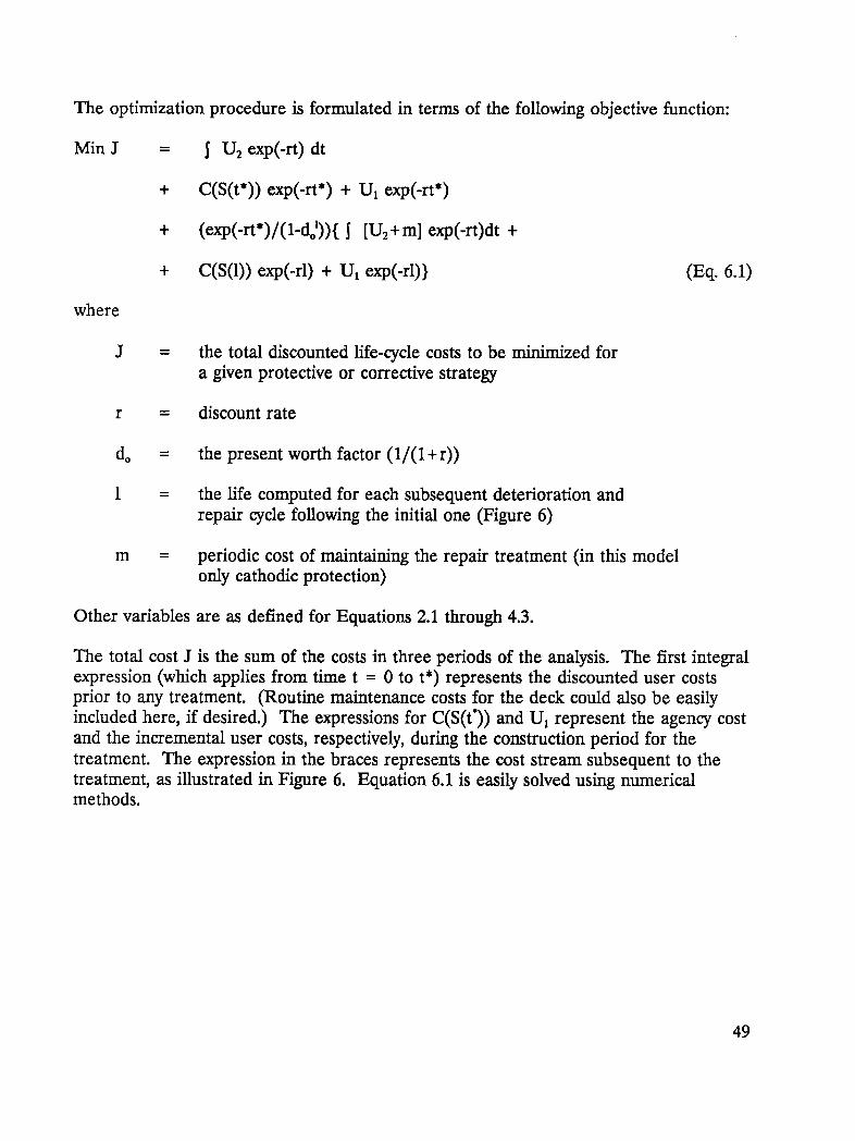
The optimization procedure is formulated in terms of the following objective function:
Min J = S U2 exp(-rt) dt
+ C(S(t*)) exp(-rt*) + UI exp(-rt*)
+ (exp(-rt*)/(1-doZ)){ i [Us+m] exp(-rt)dt +
+ C(S(1)) exp(-rl) + UI exp(-rl)} (Eq. 6.1)
where
J = the total discounted life-cycle costs to be minimized fora given protective or corrective strategy
r = discount rate
do = the present worth factor (1/(l+r))
1 = the life computed for each subsequent deterioration andrepair cycle following the initial one (Figure 6)
m = periodic cost of maintaining the repair treatment (in this modelonly cathodic protection)
Other variables are as defined for Equations 2.1 through 4.3.
The total cost J is the sum of the costs in three periods of the analysis. The first integralexpression (which applies from time t = 0 to t*) represents the discounted user costsprior to any treatment. (Routine maintenance costs for the deck could also be easilyincluded here, if desired.) The expressions for C(S(t°)) and UI represent the agency costand the incremental user costs, respectively, during the construction period for thetreatment. The expression in the braces represents the cost stream subsequent to thetreatment, as illustrated in Figure 6. Equation 6.1 is easily solved using numericalmethods.
49

6.3 Example Solutions of Optimal Deck Treatments
How the Solution Works
Interpreting of the figures below will be easier with an understanding of the numericalsolution, a simple procedure. For a given treatment, the procedure steps through theanalysis period year by year. Within each year, it performs the analysis described below.
• It simulates the application of the treatment in that year. For example, if thetreatment is a concrete overlay, the computer simulates the performance ofthe overlay in Year 1. Next, it simulates the performance of the overlay inYear 2. It continues this procedure for each succeeding year in the analysisperiod.
• As each treatment is simulated, the procedure tallies all life-cycle costs(essentially the different terms in Equation 6.1), including both the agencyand the user costs prior to the treatment, during the project to install thetreatment, and after the treatment.
• The various cost components computed above are stored in a table organizedby the year in which the selected treatment was simulated to be performed.At the end of the analysis (i.e., when costs have been tallied for all yearswithin the analysis period), the optimal solution may be obtained byidentifying the year with the lowest life-cycle costs associated with treatmentperformance.
It is very important to note that the time dimension is correlated with the condition ofthe bridge deck. Treatments that occur at the beginning of the analysis will affect thedeck in its current condition. Treatments later in the analysis will affect a deck as it hasdeteriorated from its current condition to its condition at that later point in time.
Example Data
For this example, we assumed the following as constant for all the treatments:
• A relatively new, lightly distressed bridge deck with an area of 4,000 squarefeet (372 square meters) (four lanes wide totaling 48 feet (15 meters), with alength of about 83 feet (25 meters).
• An average daily traffic volume of 25,000, with a value of time of $10 perhour.
50
• A free-flow crossing time of 0.01894 minutes (based on the bridge length of83 feet (25 meters) and a speed of 50 miles per hour (80 kilometers perhour).
• A normal two-way capacity of 96,000 vehicles per day and a capacity duringthe treatment of 57,600 vehicles per day (assuming one lane of the bridge isclosed at a time).
• No annual maintenance either of the bridge deck before the treatment, or ofany of the treatments after their installation.
• A discount rate of 5 percent.
The factors that varied in each of the cases were the characteristics of the treatments.
Four basic types of protective or corrective strategies were considered in these examples:
• Patching (i.e., patching with portland cement concrete after removingdeteriorated concrete).
• Applying a sealer after patching of deteriorated concrete.
• Applying a concrete overlay over the entire deck after patching deterioratedconcrete.
• Installing of a cathodic protection system after patching deteriorated concrete.
Key values associated with these four options are shown in Table 2. Variations in thesemethods (to reflect different types of patches, sealers, overlays, cathodic protectionsystems, or other types of treatments) would be reflected by changing the values of theparameters in Table 2 (or other parameters in the model, such as the extent of bridgeclosure).
Example of Optimal Timing
An example of the computation of optimal treatment timing is given in Figure 10 for theconcrete overlay. Figure 10 shows the life-cycle costs attributable to the simulatedperformance of the overlay treatment in each of Years 1 through 36 of the analysisperiod. Three cost curves are shown:
• Discounted agency costs attributable to performing the treatment, plus anamount for the presumed cycle of subsequent repairs (computed in lieu of asalvage value, as explained earlier).
51

• Discounted incremental user costs attributable to (1) riding on a badlydeteriorated deck and (2) delays due to congestion during the treatmentproject. These costs are tallied not only surrounding the initial treatment (forwhich the optimal solution is being computed), but also for the series ofsubsequent repairs computed in lieu of a salvage value, as mentioned above.
• Discounted total costs, representing the sum of the agency costs and the usercosts.
The agency cost curve declines over time up to a point, because of the effect of thediscount rate. A higher discount rate would result in a steeper decline over time, and alower discount rate, a more gentle decline. At about 27 years, however, agency costsbegin to increase, albeit in a very flat region of the curve. This increase occurs becausethe area of the deck requiring patching prior to overlay becomes excessive and starts todrive the costs of the treatment higher faster than the discount rate can compensate forthe increase. Thus, the agency cost curve illustrates a tension in the solution betweenthe rate of discount and the rate of deterioration of the bridge deck, and the opposingeffects of these two parameters on costs.
Table 2. Input Data for Example Treatments
Parameter Patching Sealer Concrete CathodicOverlay Protection
Service Life, 6 10 20 30
years
Cost of Patching, 35 35 35 35dollars per square foot
Project Cost (to treat 0 1,230 24,000 36,000entire deck area),dollars
Productivity, 135 135 135 135square foot per day
Time for Project to Treat 0 4 10 20Entire Deck,days
Improvement Factor 0.765 0.765 0.765 1.0(fraction of conditionimproved)
52
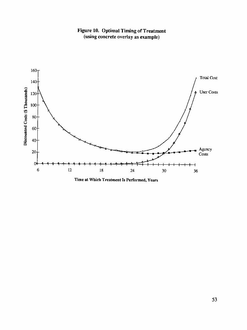
Figure 10. Optimal Timing of Treatment(using concrete overlay as example)
160t140, / Total Cost
User Costs
60.t _N_,,_ //
i / _, /_._ 40." "_,,,,:,.., ./ J
20- ,,---r.___.___.._- _ • 1/%_.__._.__._-_ Agency---_,-- Costs
.............. I I I I I
6 12 18 24 30 36
Time at Which Treatment Is Performed, Years
53

The user cost is essentially 0 throughout the early part of the analysis, indicating very fewincremental costs because the deck is new and has no adverse impacts on speed andtravel time. Congestion costs due to the treatment project are negligible in all cases andfor all years in this example, because of the relatiwfly short length of the bridge and themodest level of traffic. This situation might change with longer spans, in which traveltime effects would become more significant, or with detours around the bridge site.Implications of higher traffic volumes are investigated later in the example.
Note that the user costs do not begin to affect the result until the bridge deck conditiondeteriorates to a condition bad enough to have a noticeable effect on traffic.Furthermore, the increase in user costs may occur at relatively low values of thecondition index, S, taken over the entire deck area, since distress is likely to beconcentrated in the wheelpaths, exhibiting much higher "local" values of S. In effect,therefore, the incremental user costs act as an economic justification for bridge decktreatments. Viewed another way, the dramatically higher user costs attributable toworsening deck conditions are the penalties that drivers incur for deferred repair of afacility.
The optimal timing of the overlay treatment is obtained from the point of minimum totalcosts in Figure 10, which in this case is 24 years. This optimum is based on consideringboth agency costs and user costs. If user costs were not considered in this problem-thatis, if the decision on overlay timing were predicated solely on agency costs-the optimaltiming would have been determined to be later, in Year 27. More important, the regionof optimal timing is more clearly defined when user costs are considered. Consideringonly agency costs, the least-cost value occurs in a very fiat part of the curve, where thecosts of deferral may not be significant enough to justify expenditures against competingbridge needs. In other words, considering agency costs alone does not introduce the fullscope of the benefits of bridge treatments, or the full scope of penalties if suchtreatments are deferred or foregone.
Comparison of Treatments
Analyses such as those described above for overlays were performed for all fourtreatments listed in Table 2. The results are summarized in Figure 11, showing only thetotal cost curves for each treatment. Bear in mind that these results are for the
relatively new (and therefore only slightly distressed) bridge deck that was considered inthe example. In this light, the results are interpreted as follows:
54

Figure 11. Comparison of Treatments
100- CathodicProtection
90- _0_ verlay
80-
_ 70
60-
_ 0"._ 40-
30-
20-
10-
. Sealer0 t ,-.._ * • I i a J a.171_.. _ , I , I I I I [ I ] I I [ I , , , , i i I [ I I [ I
1 3 5 7 9 11 13 15 17 19 21 23 25 27 29 31 33 35
Time at Which Treatment Is Performed. Years
55
• The optimal time for patching occurs strictly in Year 5, although the total costcurve is so fiat that the activity would be justified virtually at any timerequired in the first 10 or 15 years. Costs are low, of course, because thedeck is relatively undamaged, so the total costs of the treatment are small,even though the unit costs (per square foot of distressed deck area) arerelatively high compared to those of the other treatments.
• The optimal time for sealer application occurs strictly in Year 16, althoughtotal discounted costs do not vary significantly within 5 years before or afterthis time. Total discounted costs in this region are somewhat more than forconcrete patching, but still relatively low.
• Both concrete overlays and cathodic protection have optimal times much laterin the deck's life, and at higher costs than for either the sealer or patching.For overlays the optimal treatment time is 24 years, as discussed earlier; forcathodic protection it is 26 years. (These treatments may show greaterbenefits in future versions of the model as more sophisticated corrosionrelationships are included for protection techniques and better data on servicelife and degree of improvement are developed through other SHRP projects. 4)
These results indicate the value of preventive and relatively small-scale correctiveactivities at this point of the deck's life cycle. Since the current level of distress is small,treatments that can correct this distress or prevent further distress at relatively low costare preferred.
Effect of Parameter Variation
The parameters identified in Table 2 can be varied to assess their impact on thesolution. To give one example, we investigated the effect of an increased traffic volume.The average daily traffic of 25,000 in Table 2 was increased to 55,000 (just below thebridge capacity during the treatment project). Results and comparison with the originalcase are shown in Figure 12, using the overlay treatment as an example.
The increase in traffic results in an earlier optimal time of treatment (from 24 to 23years) and a somewhat higher minimum total cost. Both of these effects are expectedand consistent with the problem formulation. A higher traffic volume increases thepenalties of a deck in bad condition (since more users experience this condition),prompting an earlier treatment. The higher total costs are associated with severaleffects:
• The earlier performance of the treatment, which means that the agency costsare not discounted as much.
56

• The greater number of users experiencing a deteriorating deck condition.
• Interactions among users themselves: that is if traffic speed is reducedsomewhat because of distress in the wheelpaths on the deck, the greaternumber of users increases the degree of congestion exponentially.
57
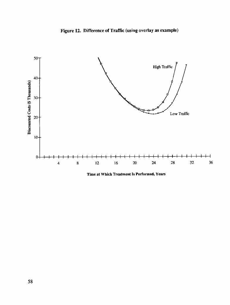
Figure 12. Difference of Traffic (using overlay as example)
50
High Traffic/ /40-
o
t--, 30-
.... • Low Traffic"_ 20-
o
10-
O l l I I I I I [ ', I [ [ [ [ [ I I I I I l I ', [ _ [ [ e I I I I I i I I
4 8 12 16 20 24 28 32 36
Time at Which Treatment Is Performed, Years
58

Appendix A
Flowcharts
59

Flowchart 1. General Technical Methodology for Technical Goal One
s_ i
GENERAL INFORMATION MODULE i
yes MODULE
Calculate & Use S r al t r
no
PROTECT INFORMATION MODULE ]
I PRESENT INFORMATION MODULE 1Calculate Sp at tp
r _ For pre_;ously repaired
L TIME-TO MODULEPOST-
DETERIORATION yes- (td) is replaced by time ofrepair (tr) and conditionSUBMODULEafter repair (S_) replaces
the tdcondition of 1.9no
Calculation One 1 DETERIORATION
Submodule SUBMODULE yes
I Define td at S=1"9 Ignore Sp&tp
no i 1Use present distress _ MODULEcondition and present Calculate & Use Sp at tp
time from present module l Time to Distress is equal to
Use Spat tp the present time;td:--tp _andSp=1.9)
__
Calculation One _ Calculation Two
Submodule Submodule
Define taat S=1.9 Define t at S=45
I........ tI
I_- I _- Fit these two points L
60 to the distress equation

Flowchart 2. General Information Module
.[ Y_r Co_ctcd? ]
iS'zof m m rI(in square feet)
Type of the member-Deck
-Substructure
I
Deck Substructure
I Loaddeck default file I Load Substructure default file
no no
yes yesV •
Add cost of overlay removal as Addcost of jacket removalasunit cost of removalmultiplied _ _ unit cost of removalmultiplied
by the areato b¢ removed ,, by the area of the jacket
yes __ no
I presentinf°rmati°nm°dule I Presentinformationmodule I

Flowchart 3. Protect Information Module
Water-cementratioof the Lconcretearoundthe bar I"
yes _s .p=O?_
!
Cannot proceed n_,no Inputwatercement ratiois out of
further.Stop _ yes _. acceptablerange1) want to input again
2) don'tknow
yes
no_ Calculate lOth
no percentile covervalue=designcover minus
0.48 in. (1.2cm)
I Howmanycoverdataareavailable? [I
tJ
[ Inutver II Calculate and standarddeviation from the inputcovervalues I
I
average
i
Calculate lOth percentile cover (average cover - ]value 1o 282 _ICstandar d deviation)
no Was this structure built with corrosion
protective system at the time of construction?
yesPRESENT
INFORMATION Please identify number of protective system used from the following listMODULE1) Epoxy-coated rebar2) Latex-modified concrete overlay3) Concrete overlay (including low-slump dense concrete)4) Full depth Silica Fume concrete5) Silica Fume concrete overlay6) Waterproof membrane with asphalt concrete overlay7) Penetrating sealer8) Surface protective coating9) Corrosion inhibitor admixture10) Cathodic protection 11) Other
User additional of service resulting from each protective system Iinputs years
62
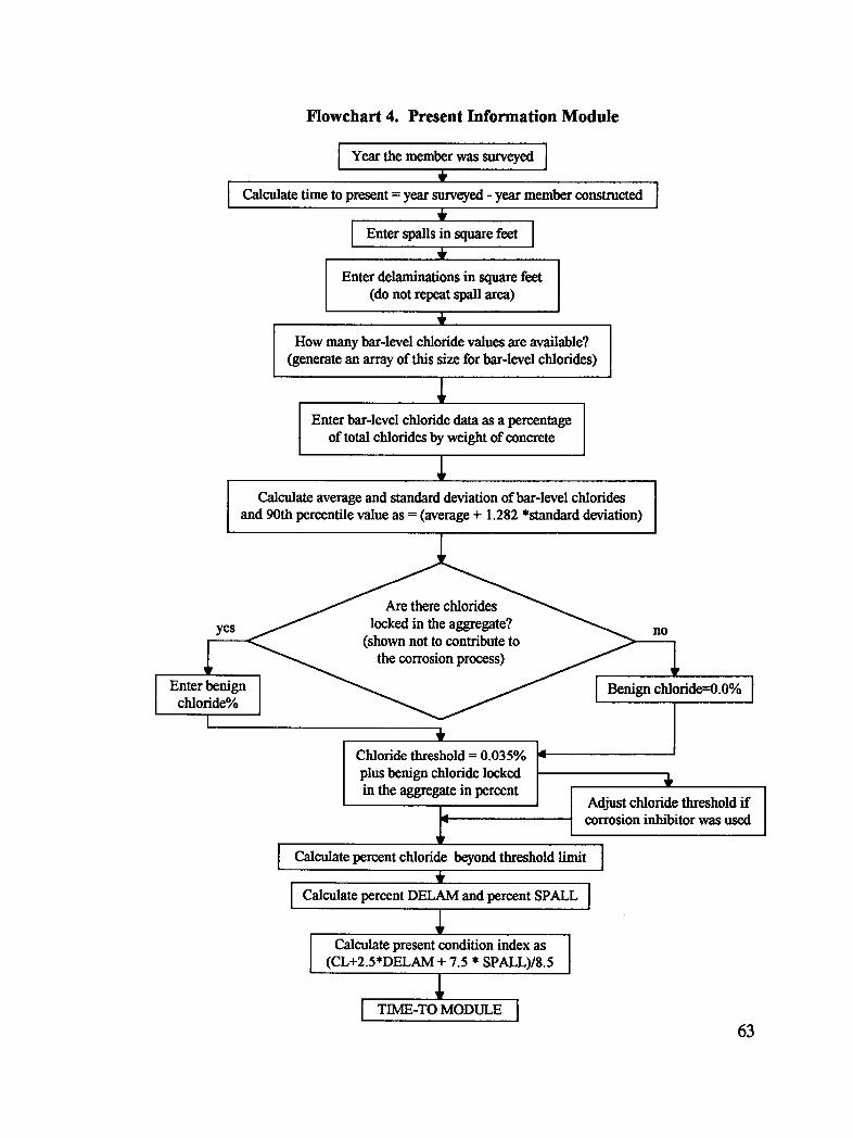
Flowchart 4. Present Information Module
Year the memberwas surveyed [i
[ Calculate time to present= yearsurveyed- yearmemberconstructed Im
! I
[ Enterspalls in squarefeet [t
Enterdelaminationsin Nl_are feet [(do not rent spall area)
How manybar-level chloridevalues are available?(generate an array of this size forbar-level chlorides)
I
Enter bar-level chloride data as a percentage [of total chloridesby weight of concrete I
!
Calculateaverageandstandarddeviationof bar-levelchlorides [and90th percentilevalueas = (average + 1.282 *standarddeviation) I
Enter benign [ _ _ I Benign chloride_.-0.0%]chloride% ]
It /
Chloridethreshold= 0.035% _1
plus benign chloride locked [ _,in the aggregatein percent
Adjustchloride thresholdff
corrosioninhibitorwas used
'[ Calculatepercentchloride beyondthresholdlimit I| I
'[ Calculate percentDELAMand percent SPALL ]i I
(CL+2.5*DELAM + "/.5* SPALL)/8.5
63

Flowchart 5. Time-to Module
I
ImportDatafrom general, [present, and protect information modules I
yes no
_ " --!
Post- Deterioration Submodule II
CalculationOne ISubmodule (Sp= 1.9)
Present condition tion module Time to distress =index and
___ present time; td = tppresenttime from for correspondingSppresent module
Calculation One
Submodule (Sp= 1.9)
iCalculationTwo
Submodule
1Fit the two points tothe distress equation
64
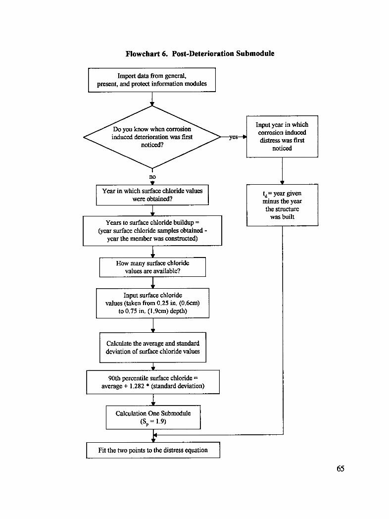
Flowchart 6. Post-Deterioration Submodule
Importdatafrom general,present, andprotect informationmodules
Inputyearin whichcorrosioninduced
yes--_ distress was firstnoticed
no LT _
Year in which surfacechloride values I td= year given
1
were obtained? I minus the year
the structurewasbuiltYears to surfacechloridebuildup=
(yearsurfacechloride samplesobtained -year the memberwas constructed)
values are available?
Input surface chloridevalues (taken from 0.25 in. (0.6cm)
m 0.'/5 in. (1.9cm) depth)
Calculate the averageand standarddeviation of surface chloridevalues
,kI
90th percentile surface chloride= Iaverage + 1.282 * (standard deviation) I
I Calculation One Submodule(Sp= 1.9)
!
Fit the two points to the distress equation ]
65

Flowchart 7. Calculation One Submodule
This module calculates the time to first deterioration, td,using the following formula
td= _J
Where
td= time to first signs of corrosion-induceddistress, yearsd =depth of barcover, inchesZt= surface chlorideconcentration,percentby weight of concretet = age at which Zt was measured,years; andP = concretewater-cementratio
66
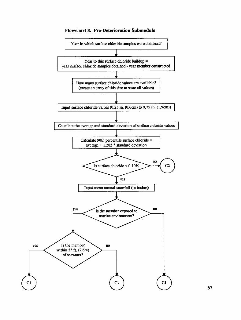
Flowchart 8. Pre-Deterioration Submodule
Year in which surfacechloridesampleswere obtained?
[ Year to this surfacechloridebuildup= [year surface chloride samplesobtained- year memberconstructed
I How manysurfacechloride values areavailable? [
I
(create an arrayof this size to storeall values) I
Input surface chloride values (0.25 in. (0.6cm) to 0.75 in. (l.9cm)) ]
Calculate the averageand standarddeviationof surfacechloride values ]
[ Calculate90th percentilesurface chloride = '1I average+ 1.282 * standarddeviation I
no
[ Input mean annual snowfall (in inches) ]
no
yes _ no
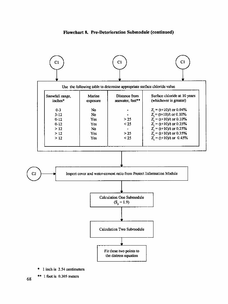
Flowchart 8. Pre-Deterioration Submodule (continued)
Use the following table to determine appropriate surface chloride value
Snowfall range, Marine Distance from Surfacechloride at 10yearsinches* exposure seawater, feet** (whichever is greater)
0-3 No - Zt = (t+10)/t or 0.04%3-12 No - Zt= (t+10)/t or 0.10%0-12 Yes > 25 Zt = (t+10)/t or 0.10%0-12 Yes < 25 Zt = (t+10)/t or 0.25%> 12 No - Zt = (t+10)/t or 0.25%> 12 Yes > 25 Zt = (t+10)/t or 0.35%> 12 Yes < 25 Zt = (t+10)/t or 0.45%
1_ q Import cover and water-cement ratio from ProtectIlfformationModule [
CalculationOne Submodule(Sp= 1.9)
lCalculation Two Subm_lule
Fit these two points tothe distress equation
* 1 inch is 2.54 centimeters
** 1foot is 0.305 meters68
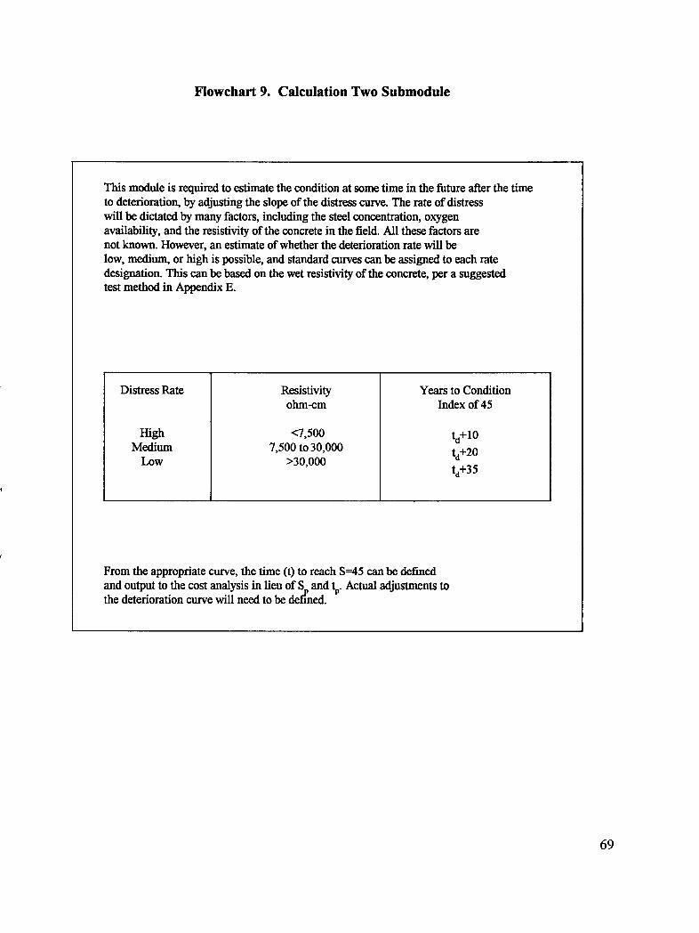
Flowchart 9. Calculation Two Submodule
This module is requiredto estimate the condition at some time in the futureafter the timeto deterioration,by adjustingthe slope of the distress curve.The rateof distresswill be dictatedby manyfactors, including the steel concentration,oxygenavailability,and the resistivityof the concretein the field. All these factorsarenotknown. However,an estimateof whether the deteriorationrate will below, medium,or high is possible,and standardcurvescan be assignedto each ratedesignation.This canbe based on the wet resistivityof the concrete,per a suggestedtestmethod in Appendix E.
DistressRate Resistivity Yearsto Conditionohm-cm Index of 45
High <7,500 td+10
Medium 7,500 to 30,000 ta+20Low >30,000
td+35
From the appropriate curve, the time (t) to reach S=45 can be defined
and output to the cost analysis in lieu of Spand tp. Actual adjustments tothe deterioration curve will need to be defined.
69

Flowchart 10. Repair Information Module
J previousrepairwas performed IYear in which
Years to previous repair=(yearin which previousrepairwas done -year in which memberwas constructed)
,I Input area of spall leftafter repair in square feet (typically zero) ']
I Inputareaof delami_tion left after repair in square feet (typically zero) '1b I
I
] Calculatepercentageof delamination(justafter repair)= (area of delarn/ areaof the member) [I
I I
i
[ Calculatepercentageof spaU(justafterrepair) = (area of spall / area of member [
i
I i
Enter approximatepercentage of member left contaminated with chloride alter repairIf exact percentage is not known, choose one of the ranges to the best of your knowledge
a) 0-15% b) 15-30% ¢) 30-50% d) 50-75% e) "/5-100%(ifa rangewas chosen, then the maximumof that range will be used forapproximatecalculations)
Calculate the condition index just after previous repair=(CL + 2.5 * DELAM + 7.5 * SPALL) / 8.5
((This index is taken as equivalent to the index at time m deterioration)
lWas any of the following protectiondone?
(1) Was a concrete overlay placed?(2) Were a membrane and asphalt concreteoverlay placed?
(3) Was a functionalcathodic protectioninstalled?(4) Was an effective sealerplaced?
(The analysiscannotbe performed ira cathodicprotection systenmhas been installed)
Fit these two points tothe distress equation
70
Appendix B
Report Format Example
71
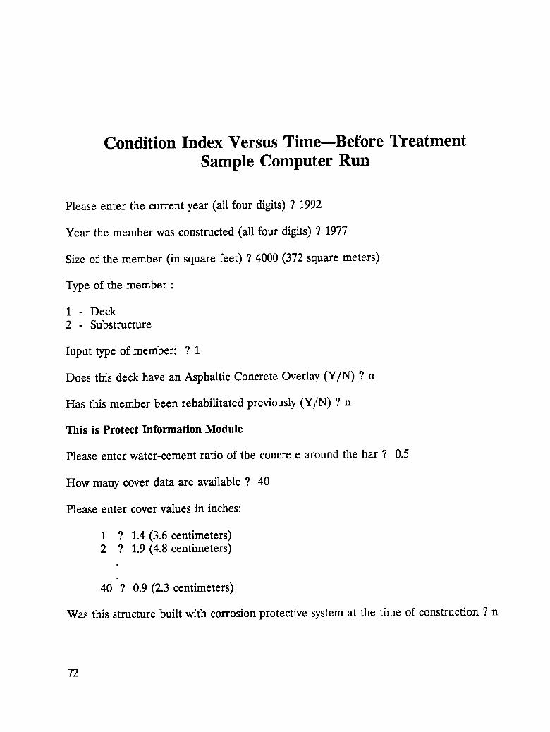
Condition Index Versus Time--Before TreatmentSample Computer Run
Please enter the current year (all four digits) ? 1992
Year the member was constructed (all four digits) ? 1977
Size of the member (in square feet) ? 4000 (372 square meters)
Type of the member :
1 Deck2 Substructure
Input type of member: ? 1
Does this deck have an Asphaltic Concrete Overlay (Y/N) ? n
Has this member been rehabilitated previously (Y/N) ? n
This is Protect Information Module
Please enter water-cement ratio of the concrete around the bar ? 0.5
How many cover data are available ? 40
Please enter cover values in inches:
1 ? 1.4 (3.6 centimeters)2 ? 1.9 (4.8 centimeters)
40 ? 0.9 (2.3 centimeters)
Was this structure built with corrosion protective system at the time of construction ? n
72
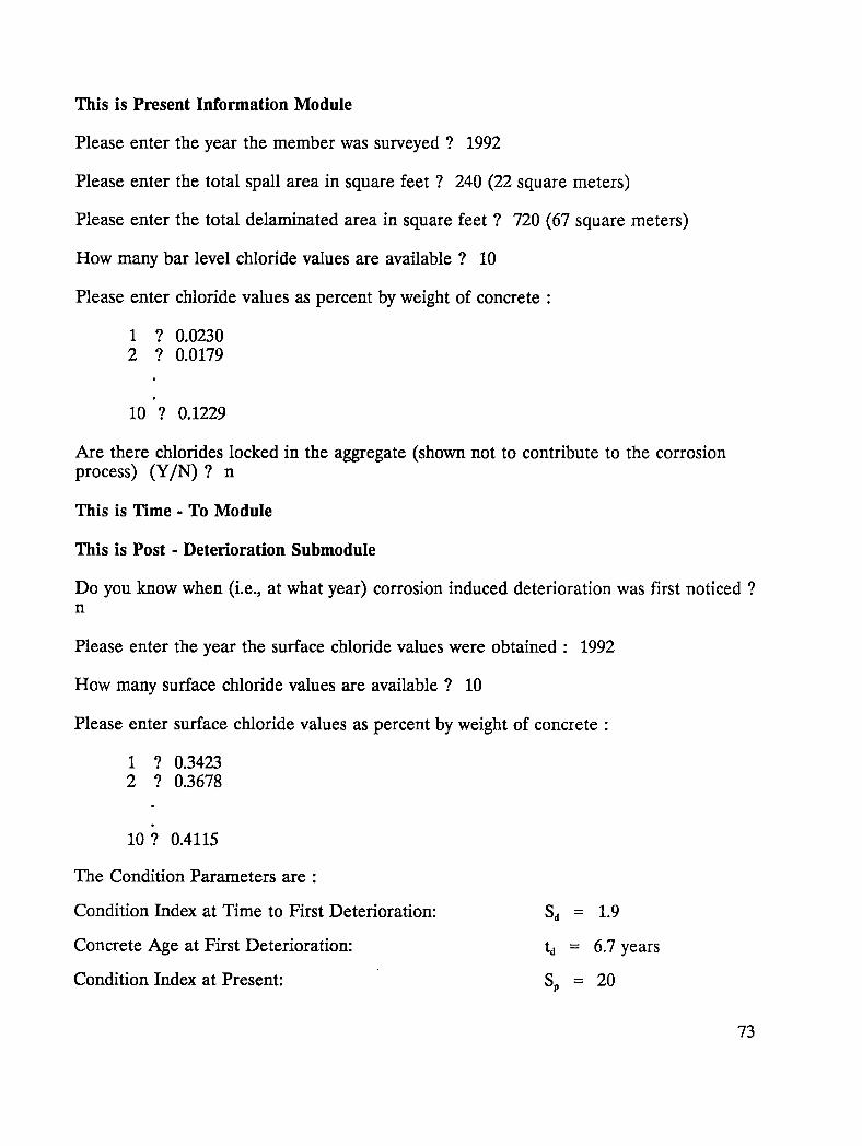
This is Present Information Module
Please enter the year the member was surveyed ? 1992
Please enter the total spall area in square feet ? 240 (22 square meters)
Please enter the total delaminated area in square feet ? 720 (67 square meters)
How many bar level chloride values are available ? 10
Please enter chloride values as percent by weight of concrete :
1 ? 0.02302 ? 0.0179
10 ? 0.1229
Are there chlorides locked in the aggregate (shown not to contribute to the corrosionprocess) (Y/N)? n
This is Time - To Module
This is Post - Deterioration Submodule
Do you know when (i.e., at what year) corrosion induced deterioration was first noticed ?n
Please enter the year the surface chloride values were obtained : 1992
How many surface chloride values are available ? 10
Please enter surface chloride values as percent by weight of concrete :
1 ? 0.34232 ? 0.3678
10 ? 0.4115
The Condition Parameters are •
Condition Index at Time to First Deterioration: So = 1.9
Concrete Age at First Deterioration: to = 6.7 years
Condition Index at Present: Sp = 20
73
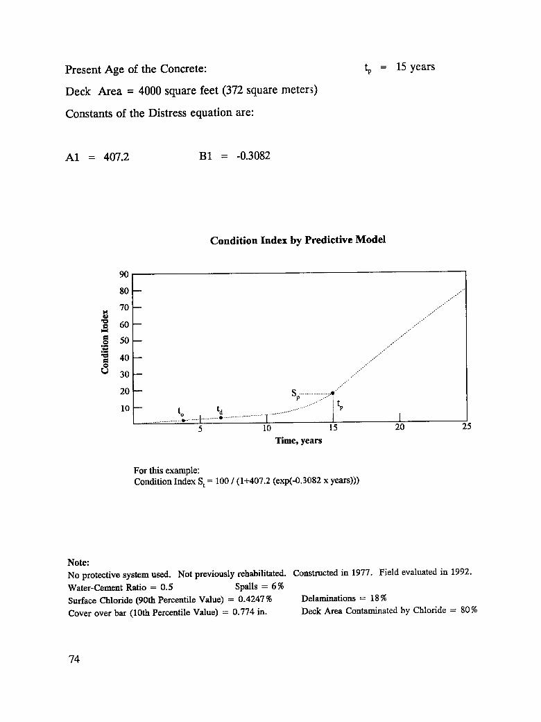
Present Age of the Concrete: tp = 15 years
Deck Area = 4000 square feet (372 square meter:s)
Constants of the Distress equation are:
A1 = 407.2 B1 = -0.3082
Condition Index by Predictive Model
90
80--.-"'"
70-- .......M
,_ •60- .......
o 50--
"= 40 ...... ".'"
30-- .........,,/
20 -- Sp.........._i"-":*'".... ......-'""""10 -- to td tp
.............° .......t.........."........................I......... I5 10 15 20 25
Time, years
For this example:
Condition Index St = 100 / (1+407.2 (exp(-0.3082 x years)))
Note:
No protective system used. Not previously rehabilitated. Constructed in 1977. Field evaluated in 1992.
Water-Cement Ratio = 0.5 Spalls = 6%
Surface Chloride (90th Percentile Value) = 0.4247 % Delaminations = 18%
Cover over bar (10th Percentile Value) = 0.774 in. Deck Area Contaminated by Chloride = 80 %
74

Appendix C
Condition Index
75

Condition Index (S)
Three major factors influence the corrosion condition of the structure at a given time
• Percent bar-level chloride contamination (CL).
• Percent delamination (DELAM).
• Percent spalling (SPALL).
Of these, spalling is the most important, delamination is second, and the bar-levelchloride contamination is the least important when considering treatment at a giventime.
The importance of each of these variables (in triggering treatment) was defined asfollows:
• Spalling is three times more important than delamination.
• Delamination is 2.5 times more important than bar level chloridecontamination.
S = CL+2.5(DELAM) +7.5(SPALL)8.5
where
CL = percent of bar-level samples withchlorides higher than the corrosionthreshold value
DELAM = percent of area with nonvisibleundersurface fractures only
SPALL = percent of area with visible deterioration
8.5 = a normalizing factor
76

Evaluate ten bar-level chloride samples per member or per 5000 square feet (465 squaremeters), whichever results in the greater number of data points. Sampling depth shall bebetween the cover depth and cover depth plus 0.5 inches (1.27 centimeters) at eachlocation.
Determine whether or not each value is greater than or equal to or less than thethreshold for corrosion by weight of concrete (0.035 percent (350 ppm), plus any chloridelocked in the aggregate, plus any corrosion inhibitor effect). Calculate the percentage ofsamples greater than or equal to the threshold. This will be the percentage of thestructure which is chloride contaminated.
The percentages of spalling and delamination are determined by surveying and mappingthe entire surface of the structure. Sample Index values for various conditions are givenin the following table.
SPALL DELAM CL Index
0 0 100 12
0 100 100 41
0 80 100 35
20 50 100 44
15 40 100 37
10 20 60 22
0 10 40 8
0 1 50 6
0 0 25 3
0 2 25 4
77

Appendix D
Time to Deterioration
79
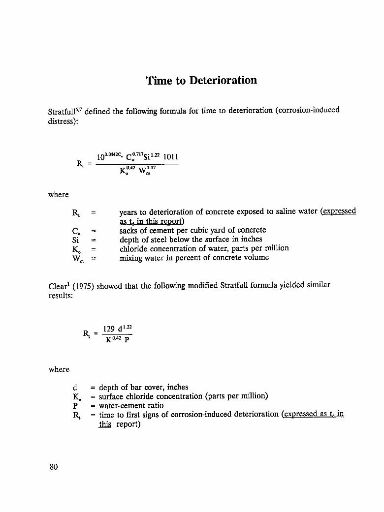
Time to Deterioration
Stratfull 6'7defined the following formula for time 1:0deterioration (corrosion-induceddistress):
10°°442c.Co°'717Si 1"22 1011R t =
Ko.42W 1.17O "'In
where
R t = years to deterioration of concrete exposed to saline water (expressedas td in this report)
Co = sacks of cement per cubic yard of concreteSi = depth of steel below the surface in inchesKo = chloride concentration of water, parts per millionWm = mixing water in percent of concrete volume
Clear 1 (1975) showed that the following modified Stratfull formula yielded similarresults:
129 d 1"22K 0-42p
where
d = depth of bar cover, inchesKo = surface chloride concentration (parts per million)P = water-cement ratio
R t = time to first signs of corrosion-induced deterioration (expressed as td inthis report)
80
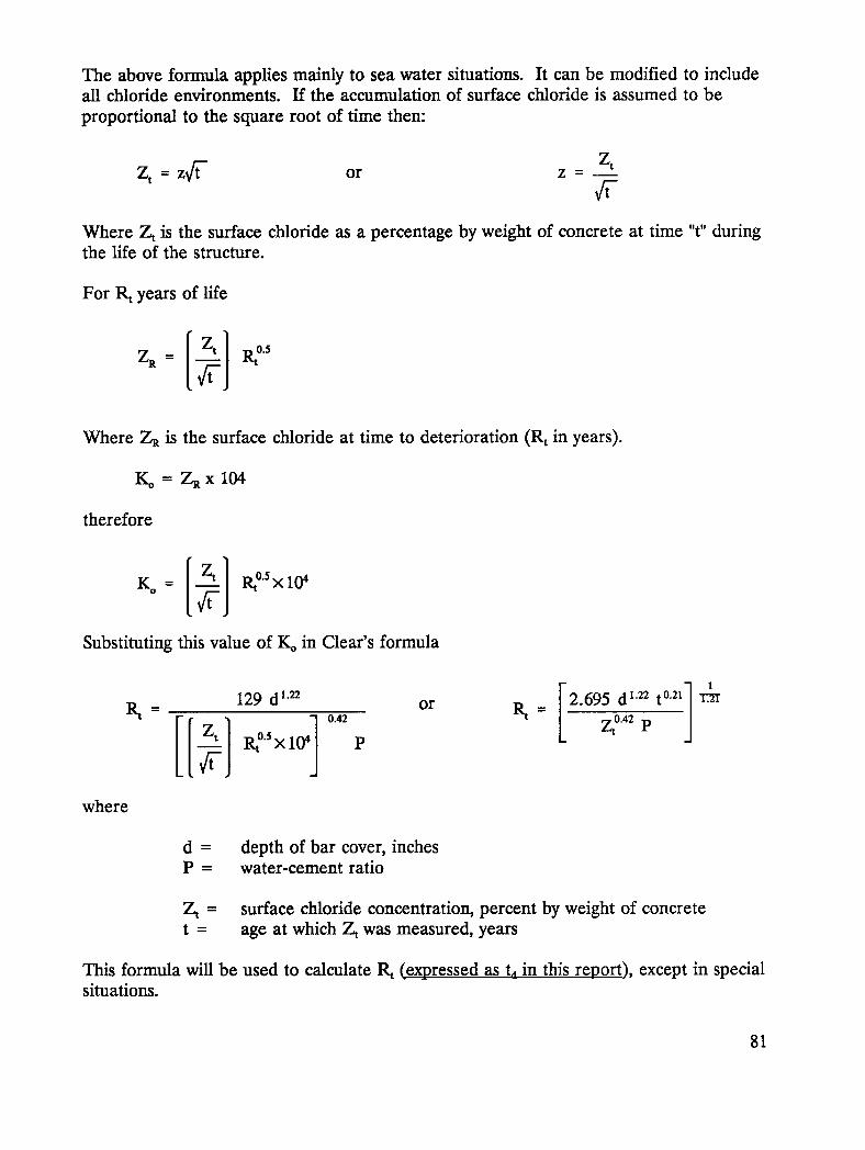
The above formula applies mainly to sea water situations. It can be modified to includeall chloride environments. If the accumulation of surface chloride is assumed to be
proportional to the square root of time then:
Z tZt -- z¢_'- or z =
Where Zt is the surface chloride as a percentage by weight of concrete at time "t" duringthe life of the structure.
For R t years of life
Where ZR is the surface chloride at time to deterioration (R t in years).
Ko = 7___x 104
therefore
Iz 1,0 ,Substituting this value of Koin Clear's formula
F ]1Rt = 129 d 1"22 2.695 d 1"22t °'21 azrr0.42 t LO'_Zt Rt°'sX1 P
where
d = depth of bar cover, inchesP = water-cement ratio
Zt = surface chloride concentration, percent by weight of concretet = age at which Zt was measured, years
This formula will be used to calculate R t (expressed as td in this report), except in specialsituations.
81

Condition index (S) at time to deterioration (td) is defined as follows:
Bar-level chloride contamination = 15 percent
Delamination = 0.5 percent
SpaUing = 0 percent
Condition index at ta = So = 1.9
Time to Corrosion Initiation, to
If to > 20 years, t. = to- 5If t0 = 10 to 20 years, to = td" 3.5If t0 < 10 years, to = to - 2
Condition index at t. = S° = 1.2(10 percent chloride contamination, 0 percent delamination, and 0 percentspalling)
82

Appendix E
Calculation Two Submodule
83

Calculation Two Submodule
Average Wet Resistivity, Years to Condition ]index of Distress Rate*ohm - cm** 45 percent (percent index increase per
year)
< 7,500 ta + 10 4.31
7,500 to 30,000 h + 20 2.16
>30,000 h + 35 1.23
* Distress Rate (percent index increase per year) is calculated as follows:
Condition Index- 1.9
Years to Condition Index-t a
For example the distress rate for medium resistivity concrete is:
(45 - 1.9) _ 43.1 _ 2.16(td + 20-td) 20
**ESTIMATED ELECTRICAL RESISTIVITY OF CONCRETE MATERIALS
Obtain three fully cured core or cylinder samples at least 4 inches (10.2 centimeters) in diameterand 2 inches (5.1 centimeters) long. The samples shall be completely representative of theconcrete to be studied.
Perform Rapid Permeability tests on each of the three samples in accordance with the procedureof AASHTO T277-83I "Rapid Determination of the Chloride Permeability of Concrete", exceptadd the following:
Immediately prior to connection of the 60-volt power supply leads, record the two pin ACresistance between the two cell halfs, measured with a Nilsson 400 or equivalent.
Calculate estimated resistivity by multiplying the measured AC resistance by 16.8.
84

Report the estimated resistivity (73 degrees F, vacuum saturated) for each specimen. Averagethe findings for the three individual specimens and also report the average and the range.
85

86

\
\
;=¢
0
\ ",_ o_
• 0 _ ", C)
*
_ ""-. l
",,
I I I I I I I I I _
_,_ 0'_ _ I_ _0 _ '_ e,_ _,l _
xspuI uo!_!puo_3
87
Appendix F
Criteria for Preventive Maintenance
89
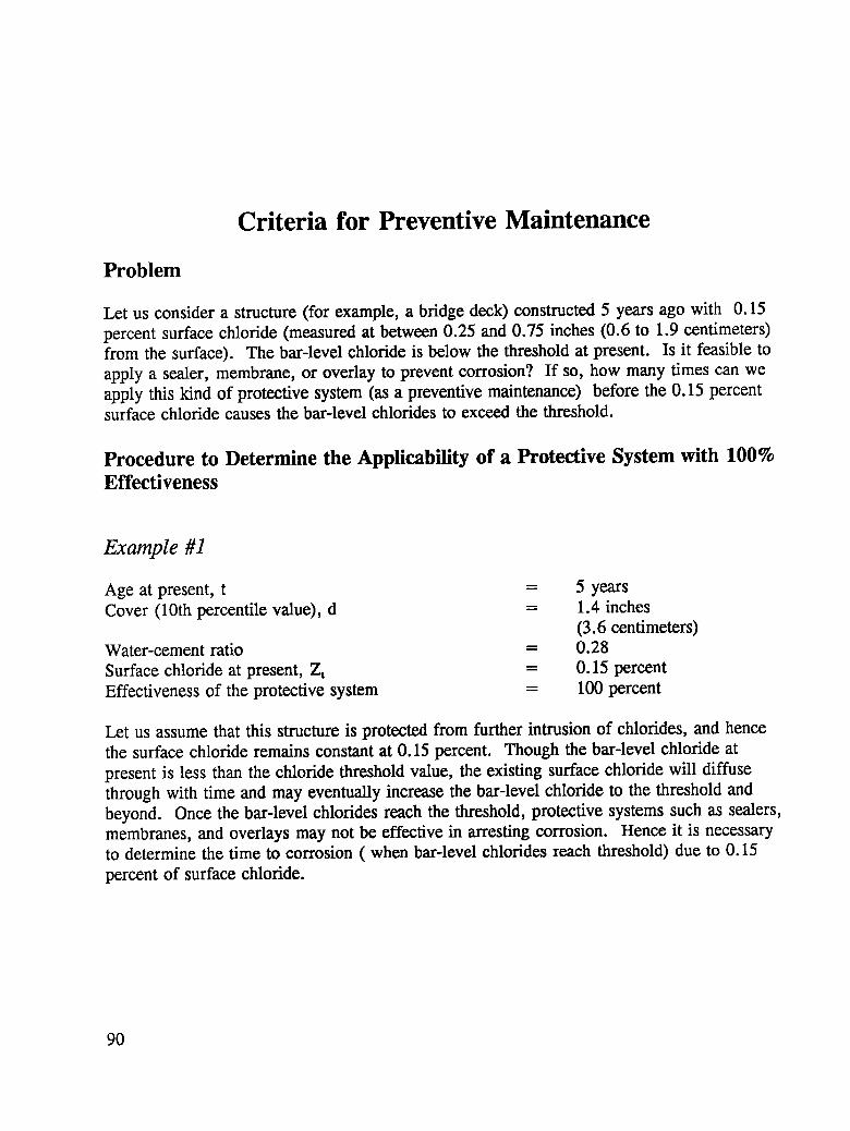
Criteria for Preventive Maintenance
Problem
Let us consider a structure (for example, a bridge deck) constructed 5 years ago with 0.15percent surface chloride (measured at between 0.25 and 0.75 inches (0.6 to 1.9 centimeters)from the surface). The bar-level chloride is below the threshold at present. Is it feasible toapply a sealer, membrane, or overlay to prevent corrosion? If so, how many times can weapply this kind of protective system (as a preventive maintenance) before the 0.15 percentsurface chloride causes the bar-level chlorides to exceed the threshold.
Procedure to Determine the Applicability of a Protective System with 100%Effectiveness
Example #1
Age at present, t = 5 yearsCover (10th percentile value), d = 1.4 inches
(3.6 centimeters)Water-cement ratio = 0.28Surface chloride at present, Zt = 0.15 percentEffectiveness of the protective system = 100 percent
Let us assume that this structure is protected from further intrusion of chlorides, and hencethe surface chloride remains constant at 0.15 percent. Though the bar-level chloride at
present is less than the chloride threshold value, the existing surface chloride will diffusethrough with time and may eventually increase the bar-level chloride to the threshold andbeyond. Once the bar-level chlorides reach the threshold, protective systems such as sealers,membranes, and overlays may not be effective in arresting corrosion. Hence it is necessaryto determine the time to corrosion ( when bar-level chlorides reach threshold) due to 0.15
percent of surface chloride.
90
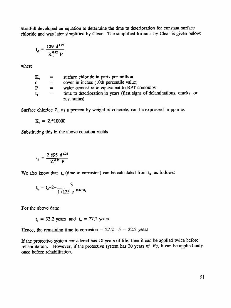
Stratfull developed an equation to determine the time to deterioration for constant surfacechloride and was later simplified by Clear. The simplified formula by Clear is given below:
129 dl_atd -
K0.42 pO
where
Ko = surface chloride in parts per milliond = cover in inches (10th percentile value)P = water-cement ratio equivalent to RPT coulombst0 = time to deterioration in years (first signs of delaminations, cracks, or
ruststains)
Surface chloride Zt, as a percent by weight of concrete, can be expressed in ppm as
Ko = Zt*10000
Substituting this in the above equation yields
2.695 d 1"22
td - Zt0.42p
We also know that to (time to corrosion) can be calculated from t0 as follows:
3to = ta-2-
1+125 e-°32_9"
For the above data:
td = 32.2 years and to= 27.2 years
Hence, the remaining time to corrosion = 27.2 - 5 = 22.2 years
If the protective system considered has 10 years of life, then it can be applied twice beforerehabilitation. However, if the protective system has 20 years of life, it can be applied onlyonce before rehabilitation.
91
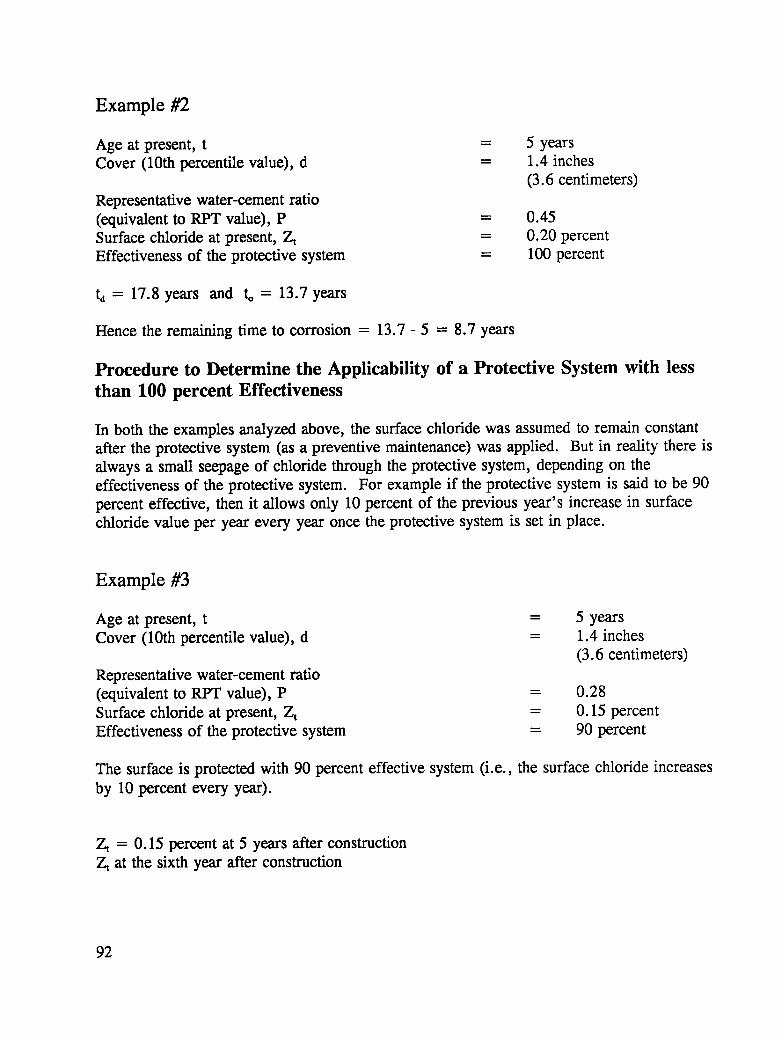
Example #2
Age at present, t = 5 yearsCover (10th percentile value), d = 1.4 inches
(3.6 centimeters)
Representative water-cement ratio(equivalent to RPT value), P = 0.45Surface chloride at present, Zt = 0.20 percentEffectiveness of the protective system = 100 percent
4 = 17.8 years and to = 13.7 years
Hence the remaining time to corrosion = 13.7 - 5 = 8.7 years
Procedure to Determine the Applicability of a Protective System with lessthan 100 percent Effectiveness
In both the examples analyzed above, the surface chloride was assumed to remain constantafter the protective system (as a preventive maintenance) was applied. But in reality there isalways a small seepage of chloride through the protective system, depending on theeffectiveness of the protective system. For example if the protective system is said to be 90percent effective, then it allows only 10 percent of the previous year's increase in surfacechloride value per year every year once the protective system is set in place.
Example #3
Age at present, t = 5 yearsCover (10th percentile value), d = 1.4 inches
(3.6 centimeters)
Representative water-cement ratio(equivalent to RPT value), P = 0.28Surface chloride at present, Z t = 0.15 percentEffectiveness of the protective system = 90 percent
The surface is protected with 90 percent effective system (i.e., the surface chloride increasesby 10 percent every year).
Zt = 0.15 percent at 5 years after constructionZ_ at the sixth year after construction
92
--o.15+_.15o15_]_Jo.loSimilarly Zt at time to deterioration
=0.15 �[0.15°155v_:il0.10(_-t)t v_ J
or in general terms
" z, lo= Zt + t _ J (t(l-t)
where e = (100 - effectiveness in percent)/100
Surface chloride in parts per million:
K = Zt + e (t,t -' v_J
Substituting this surface chloride expression in Clear's formula yielded:
2.695 d 1"22td = 0.42
[ (td - t) e (V_ - _z-f).]Zt°'42 P 1 +
v_Using the data above
td = 31years and to =26years
Hence, the remaining time to corrosion = 26 - 5 = 21 years.
93

Example #4
Age at present, t = 5 yearsCover (10th percentile value), d = 1.4 inches
(3.6 centimeters)Representative water-cement ratio(equivalent to RPT value), P = 0.45Surface chloride at present, Zt = 0.20 percentEffectiveness of the protective system = 90 percent
Using the data above data,
t_= 17 years and to= 13 years
Hence, the remaining time to corrosion = 13 - 5 = 8 years.
Comments:
The variable effectiveness formula is slightly more accurate. However, since all protectivesystems in consideration should be 90 percent or more effective, we believe that procedure#1 (assuming 100 percent effectiveness) is an adequate approximation. Remember, however,that the life of a preventive maintenance overlay is the time it completely blocks chlorideintrusion into the base concrete ( and not its physical life ).
94
PART II--HANDBOOK
1. Introduction
1.1 Purpose
In order to minimize the cost of repairing or replacing of deteriorating concrete bridgesat the network level, it is essential that cost-effective actions be taken at the projectlevel. This handbook provides a systematic methodology to guide technical personnel ofhighway agencies in determining rational, cost-effective strategies for treating specificconcrete bridge components. The output from the methodology answers the user'squestions regarding the type and timing of treatment to achieve the lowest life-cycle cost.
1-2 Approach
The methodology takes the following factors into account in conducting life-cycle costanalysis:
1. The condition of the concrete component and its performance,
2. The technical compatibility, cost, and service life of the range of treatmentalternatives from which the selection can be made.
The procedures in the handbook are devised on the basis of the concepts developed inPart I of this document. The results of SHRP research by Cady and Gannon _ were usedto make a reliable determination of the condition of the concrete. Also, the SHRPresearch by Weyers et. al.4was used to develop concepts for determining concrete servicelife. Both agency costs and user costs have been taken into consideration in conductinglife-cycle analysis.
1.3 Scope
The methodology in its present form only applies when the predominant concretedeterioration is associated with chloride-induced corrosion of the reinforcing steel.
95

The procedures outlined in the handbook are primarily devised for exposed concretes,but they also apply to covered concretes. Where a procedure does not apply to coveredconcretes, adjustments have been made for covered concretes and explained.
The procedures in the handbook determine the life-cycle cost when the concrete istreated at the present or in the future. Those procedures, however, can be employed todetermine the life-cycle cost if the concrete was treated in the past. Of course, the latterlife-cycle cost information cannot be used for plarttting a treatment. However, it couldbe used to compare strategies.
The methodology is designed to be flexible and can be tailored to suit the needs of theindividual highway agencies. The user has the option of deleting those aspects of themethodology that are irrelevant to a specific case.
96

2. Overview of the Handbook
This chapter provides the user with an overview of the handbook and prepares the userfor the details of the methodology that follow in the next 11 chapters. Those 11 chapters(i.e., Chapters 3 through 13 of the handbook) provide a step-by-step procedure to leadthe user to the appropriate treatment of a specific concrete component: that is, what typeof treatment to apply, and when to apply it for maximum cost-effectiveness. The answeris obtained by conducting the life-cycle cost analyses found in Chapter 13. Chapters 3through 12 are background chapters and provide the necessary information on servicelives and costs that are input into Chapter 13 to conduct life-cycle cost analyses. Chapter14 includes an example with calculations and illustrates how the methodology is appliedto a realistic bridge component.
2.1 How to Use the Handbook
To use this handbook, the user should first become familiar with the methodology byreviewing Chapters 3 through 13. Chapter 13 can then be used for any specific case todetermine the most cost-effective strategy. In Chapter 13, references are systematicallymade to Chapter 3 through 12 to gather the input information required. The nextseveral pages outline and briefly discuss Chapters 3 through 13.
2.2 Chapter 3: Service Life Limitation due to Functional Features
This chapter addresses functional features of the bridge, so that if the remaining servicelife of the whole structure is unusually short because of functional features, that will betaken into account later, when making a decision on the component treatment. This isimportant, since the methodology employs life-cycle cost analysis to determine the mostcost-effective treatment strategy.
2.2 Chapter 4: Testing Concrete
This chapter provides the user with a guide for obtaining site-specific test data that areessential to the methodology. The following tests are needed:
97
• Visual survey and detection of spalls.• Delamination detection.• Bar cover depth measurement.• Chloride content measurement.
The following tests are only needed when the concrete presents certain conditions:
• Half cell potentials survey.• Rate of corrosion measurement.• Permeability/resistivity measurement.
2.3 Chapter 5: Condition Determination
Chapter 5 deals with determining the condition of concrete. The chapter presents asystematic procedure to employ the test data obtained in Chapter 4 to quantify thecondition in terms of an index (condition index of 100 or lower). The test dataemployed relate to spalling, delamination, and chloride contamination of the concrete.
As a concrete bridge component ages, its condition gradually changes and its conditionindex increases to a point where some type of treatment must be done. The conditionindex corresponding to the "must" condition will be selected by the user on the basis ofstructural considerations and/or the ride quality of the deck. The chapter recommends adefault value for the maximum tolerable condition index.
2A Chapter 6: Prediction of Performance
In this chapter a systematic procedure is presented for predicting the condition index ofconcrete at any given time in the future. This is done through a performance equationthat relates fire condition index to the age of concrete. There are two parameters in theequation which are systematically determined from the site-specific data. Nomogramshave been prepared as an alternative to hand calculations _:odetermine the twoparameters of the performance equation.
2.5 Chapter 7: Evaluation of Performance
Chapter 6 established a performance equation which relates the concrete condition tothe age of concrete. Chapter 7 will assist the user to understand the rate ofdeterioration of the concrete by illustrating the equation graphically. On the basis of twoparameters of the performance equation obtained in Chapter 6, the user will select theperformance curve from a family of curves.
From the performance curve, the user will define the period of time between presenttime and time corresponding to the maximum tolerable condition index (determined
98

from Chapter 5). This is the "treatment consideration period." The rest of the handbookis used to determine the timing of the treatment within the "treatment considerationperiod," as well as the type of the treatment, for maximum cost-effectiveness.
2.6 Chapter 8: Compatible Treatment Alternatives
This chapter will provide a range of treatment alternatives from which the selection canbe made. Prior to selecting all of the treatment alternatives in this chapter, the user willconsult the tables provided, screening out those alternatives which are not compatiblewith the concrete because of their technical disadvantages.
2.7 Chapter 9:. Cost Items Associated with Treatment (Agency Costs)
Costs associated with various treatments should be known so that life-cycle cost analysiscan be conducted. Cost can vary significantly from one area to another depending onmany factors. The user generally has most reliable information regarding cost of acertain treatment in a given jurisdiction. However, before the user arrives at any cost fora treatment, the standard cost items associated with that treatment must be identified.
Chapter 9 will provide standard highway agency cost items associated with eachtreatment covered in the handbook.
2.8 Chapter 10: Cost Items Associated with Treatment (User Costs)
Two types of user costs are considered in this chapter: (1) prior-to-treatment costs (decksonly), and (2) during-treatment costs. Costs in the period prior to the treatment are afunction of the condition of the bridge deck and its effect on traffic flow. A badlyspalled deck would impede traffic flow, causing speed reduction, and congestion andresulting in increased travel time and cost. Costs during the treatment are related toincreases in travel time caused by traffic congestion on the bridge or by detours aroundthe bridge during bridge closure. Nomograms are provided for determining the usercosts, as an alternative to the equations.
2.9 Chapter 11: Decomposing Concrete Condition Index
In order to estimate agency costs and user costs associated with a treatment (Chapters 9and 10), the amount of concrete repair (removal and replacement of deteriorated andpossibly contaminated concrete) needs to be predicted at the time of treatment. Theamount of deterioration and contamination in the future can be predicted bydecomposing the future concrete condition index into its component parts (i.e., chloride
99

contamination, delamination, and spalling). This chapter will provide a systematicprocedure for decomposing the condition index.
2.10 Chapter 12: Prediction of Performance after Treatment
The methodology employs life-cycle cost analysis to determine cost-effectiveness.Therefore, the service life of the concrete after the treatment, also, needs to bepredicted. Generally, two factors affect the performance of the concrete after thetreatment. Those are (1) the inherent corrosion mechanism active at the time oftreatment, and (2) the treatment's effect on the future corrosion process.
Chapter 12 uses the concept of "trend in the rate of corrosion after treatment" todetermine the effective service life of the concrete after the treatment. Equations andnomograms, as alternatives to the equations, are presented for this purpose. Theprocedure does not depend on the actual rate of corrosion, unless concrete presentscertain conditions.
2.11 Chapter 13: Optimum Treatment and Time of Treatment
Having determined: (1) the concrete performance, (2) the "treatment considerationperiod," (3) compatible treatment alternatives, (4) how to determine costs associated witha treatment, and (5) the performance after the treatment, the user must decide what typeof treatment to apply and when to apply it within the "treatment consideration period,"for maximum cost-effectiveness. Chapter 13 deals with this subject through life-cycle costanalysis.
The user will first determine for each compatible treatment the optimum time oftreatment and then will compare the corresponding life-cycle costs in order to prioritizethose compatible treatments. This is discussed below.
For simplicity, for each compatible treatment, the user will consider treating the concretecomponent at three points during the treatment consideration period: (1) the presenttime, (2) the time corresponding to the maximum tolerable condition index, and (3)some time between those two.
The economic analysis of the three possible strategies described will be done within a settime frame called the "planning horizon." The planning horizon begins with the presenttime and extends for 20 years. However, if the service life of the component is limitedbecause of the bridge's functional features, the planning horizon will be the remainingservice life of the structure, as discussed in Chapter 3.
All costs associated with each strategy, including the cost of repeated cycles of treatmentwithin the planning horizon are then discounted and totaled for comparison with theother strategies. At the end of this economic analysis, the user will be able to determine
100

the optimum strategy (time of the treatment) for a compatible treatment. Also, the userwill be able to prioritize the various compatible treatments based on their life-cycle costs.A worksheet has been prepared to facilitate life-cycle cost analysis.
101

3. Service Life LimitationDue to Functional Features
If, when the current criteria for serviceability are applied, the bridge will be functionallyobsolete in the near future, then the component treatment must be compatible with theremaining life of the structure as a whole. Life-cycle costs of various strategies can beaffected by the remaining service life of the structure, as discussed in Chapter 13.
Bridge functional features that can limit the remaining service of a bridge include
• width,
• clearance,
• alignment, and
• load limits.
The user should estimate the remaining service life of the bridge if the bridge functionalfeatures limit the remaining service life to 30 years or less. If the exact remainingservice life is not known, one of the ranges shown below may be chosen to the best ofthe user's knowledge.
• 0 - 5 years
• 5- 10 years
• 10-15 years
• 15-20 years
• 20-25 years
• 25-30 years
If a range is chosen, then the maximum of that range will be used as the remainingservice life in Chapter 13.
103

If the remaining service life is estimated at higher than 30 years, it may be assumedunlimited for the purpose of life-cycle cost analysis in this handbook.
104
4. Testing Concrete
This chapter guides the user through obtaining site-specific test data that are essential tothe methodology. Tests included in this chapter are discussed in detail in SHRPresearch by Cady and Gannon 3 and other sources cited in this handbook. Those testsinvestigate concrete element deterioration due to reinforcement corrosion. If non-corrosion deterioration is identified as significant, this handbook may not produce viableresults.
4.1 Tests Required
The tests required, and the order in which they are conducted, are given in Figure 4.1.First, a visual examination of the member is conducted to determine the area of concretespalling and to determine if other non-corrosion related deterioration is present. Next,the amount of concrete delamination (internal concrete cracking caused by barcorrosion) is obtained. This quantity does not include spalls. Third, a bar cover depthsurvey is conducted, and bar electrical continuity within the element is determined.Fourth, concrete chloride content profiles are obtained. The profiles give chloridecontent at the surface and at the bar level. Fifth, a half cell corrosion potential survey isconducted to obtain areas of highest potential. Sixth, rate of corrosion is determined inthe areas of highest half cell potential. Note that the fifth and sixth activities (i.e., halfcell test and rate of corrosion test) are generally not required (except where concretewas repaired/rehabilitated, previously); however, they are performed to support, andmodify if necessary, concepts used in the methodology. Also, those two activities neednot be considered when less than 10 percent of the bar-level chloride contents aregreater than, or equal to, the corrosion threshold chloride content.
Additionally, testing concrete for chloride permeability and/or resistivity may be requiredwhen
1. water-cement ratio of the concrete is not known (testing the concrete forpermeability),
2. permeability of a special concrete, overlaying the concrete, is questionable(testing the overlay for permeability), and
105

Figure 4.1. Tests Required
Visual Examination 1Spalling & OtherDefects
lDelaminationSur,,ey 2
'r
BarCoverSurvey 3&
BarContinuity
r
ChlorideContent I 4Surface & BarLevel
--Yes-D Half Cell 5Potential
Rate of 6
No _ Corrosionl_ChloridePermeability ConcreteResistivityWhen Representative When Corrosion 7
W/C Ratio Is not DeteriorationHas NotKnown Begun
106
3. the concrete has not yet shown the first sign of corrosion-induced deterioration(testing the concrete for resistivity).
4.2 Number of Tests and Samples
The procedures in Table 4.1 are given with suggestions for the number of tests andsamples to obtain from various bridge components.
4.3 Test Descriptions
The following chapters discuss the individual evaluation methods.
Visual Examination
A visual examination of the concrete surface is used to determine the extent of
deterioration and forms the basis for the subsequent concrete condition surveys. Thevisual examination described here is not related to the bridge survey system adopted byFederal Highway Administration s. The visual examination notes both corrosion and non-corrosion related deterioration. It should note size, location, and orientation of
1. spalls,2. patches (temporary and permanent),3. scaling,4. pop-outs,5. cracks, and6. wheeltrack wear (only bridge decks).
These items should be shown on a sketch. A grid layout is established on the concretesurface to map concrete deficiencies and to determine their magnitude based on apercent of surface area. The severity of the deterioration should be determinedquantitatively during a visual examination by simply measuring the depth of spalls,scaling, and wheeltrack wear. Exposed and corroding reinforcing steel should also benoted.
The visual examination generates a comprehensive condition survey of the concretesurface. It determines the extent of corrosion-induced spalling, as well as thesignificance of deterioration caused by reasons other than corrosion of the reinforcingsteel. The output of this procedure for use in the calculations is the percent of the areawhich has spalls, temporary patches covering spalls (e.g., asphalt patches), andpermanent patches (e.g., concrete patches).
This methodology cannot be used to determine remedial actions for non-corrosion-related deterioration (e.g., scaling, pop-outs, surface cracking, and wheeltrack wear). If
107
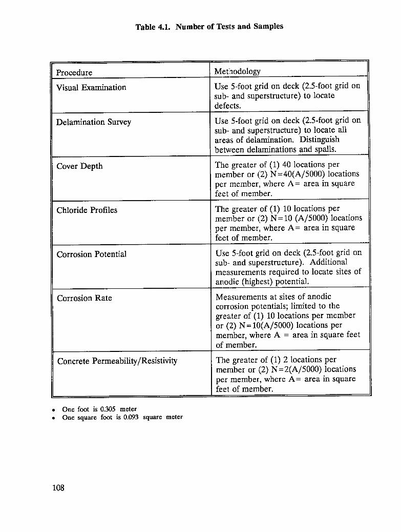
Table 4.1. Number of Tests and Samples
Procedure Methodology
Visual Examination Use 5-foot grid on deck (2.5-foot grid onsub- and superstructure) to locatedefects.
Delamination Survey Use 5-foot grid on deck (2.5-foot grid onsub- and superstructure) to locate allareas of delamination. Distinguishbetween delaminations and spalls.
Cover Depth The greater of (1) 40 locations permember or (12)N=40(A/5000) locationsper member, where A = area in squarefeet of member.
Chloride Profiles The greater of (1) 10 locations permember or (2) N= 10 (A/5000) locationsper member, where A= area in squarefeet of member.
Corrosion Potential Use 5-foot grid on deck (2.5-foot grid onsub- and superstructure). Additionalmeasurements required to locate sites ofanodic (highest) potential.
Corrosion Rate Measurements at sites of anodiccorrosion potentials; limited to thegreater of (1) 10 locations per memberor (2) N = 10(A/5000) locations permember, where A = area in square feetof member.
Concrete Permeability/Resistivity The greater of (1) 2 locations permember or (2) N=2(A/5000) locationsper member, where A= area in squarefeet of member.
• One foot is 0.305 meter
• One square foot is 0.093 square meter
108

non-corrosion-related deterioration is significant, the most cost-effective treatment maybe obtained by considering factors which are not covered in this methodology.
Delamination Survey (ASTM D4580)
This test (ASTM D4580) is used to survey concrete by sounding the surface to determinethe presence of delaminations (corrosion-induced internal cracks). To conduct this test,first a grid layout is established on the concrete surface. Second, the surface is soundedand delaminations noted. Third, the areas of delamination are marked and mapped forthe report. Fourth, the amount of delamination is computed as a percentage of thesurface area. Spalls are not included.
Where rigid overlays are applied, the test (ASTM D4580) shall distinguish delaminationsfrom debonding of the overlay. Where asphalt concrete overlays are applied,delaminations and/or debonding should be detected using the procedure recommendedby SHRP's test method, "Standard Test Method for Assessing the Condition of Asphalt-Covered Bridge Decks Using Pulsed Radar." The SHRP test method is documented inAppendix B of Cady and Gannon. 3
If overlay debonding is significant, the most cost effective treatment may be obtainedconsidering factors which are not covered in this methodology.
Cover Depth over Reinforcement Using a Cover Meter (Magnetic Flux Device)
This device uses a magnetic field to detect reinforcing steel within hardened concrete. Itcan determine the location, orientation, size, and depth of the bar. The accuracy of thedevice in measuring the depth of cover decreases as the depth of cover increases.Magnetic particles in the concrete can influence the measurements. Thus, a correctionfactor should be obtained by exposing the bar at one location and measuring the actualdepth. Usually, the correction factor is obtained at a location which can later serve asthe half cell test bar ground connection.
If the bar size is not known, the depth cannot be read directly from the scale; therefore,the following technique is suggested.
1. Locate the bar in the test area.
2. Place a two-by-four or other non-metallic spacer, between the probe and theconcrete surface.
3. Record possible bar size and depth combinations.
4. Correct readings for the thickness of the spacer by subtracting its thickness.
109
5. Place the probe directly on the concrete surface and record possible reading.
The bar size for which the same cover depth is obtained in Steps 4 and 5 is the correctresult.
Reinforcing Steel Electrical Continuity
Electrical continuity of the reinforcing steel should be known prior to conducting certaintests or applying certain treatments. Electrical continuity can be determined bymeasuring the resistance between widely separated steel components. Low resistivitiesindicates continuity.
Chloride Profiles (AASHTO T260-84, or SHRP Modified Test Method)
This test determines the chloride content of concrete. Concrete powdered samples arecollected with a vacuum bit near the concrete surface (0.25 inch to 0.75 inch (0.6centimeters to 1.9 centimeters) depth) and at the level of the reinforcing steel (thebottom 0.25 inch (0.6 centimeters) of concrete cover). Where a concrete overlay isapplied, "concrete surface" is the surface of the overlay.
The SHRP "Standard Test Method for Chloride Content in Concrete Using the SpecificIon Probe" is documented in Appendix F of Cady and Gannon. 3In the SHRP testmethod, which is a field method, the powdered samples are dissolved in, and stabilizedby, two solutions. A probe is then inserted into the mixture and the readings arerecorded in the field. Calculations convert readings into chloride content expressed as apercentage of concrete weight.
AASHTO T260-84 test method may be used for chloride content determination.
Corrosion Potential Survey (ASTM C876)
This procedure (ASTM C876) determines the potential for the existence of reinforcingsteel corrosion through measuring the electrical potential of the reinforcing steel. It maybe performed if 10 percent of the chloride samples at the depth of the steel are greaterthan the corrosion threshold chloride content.
The procedure for administering this test follows:
1. Establish a grid on the concrete surface.
2. Provide an electrical connection to the steel (ground).
110
3. Place a half cell corrosion detection device on the concrete surface at the gridpoints.
4. Record the electrical potential readings.
Note that the test cannot be conducted in the absence of the electrical continuity of thereinforcing steel.
This procedure obtains the location of highest half cell potentials (peak negativepotentials) for the subsequent rate of corrosion testing. The location of highest potentialscan be obtained in the field by scanning the concrete surface around the anodic areaswith a half cell device. The locations of anodic areas are obtained by plotting the gridhalf cell potentials and drawing equipotential contour lines.
The corrosion potential survey is not recommended for epoxy-coated or galvanizedreinforcement. This is because epoxy-coated bars are electrically insulated from eachother, and readings on galvanized bars indicate the potential of the zinc coating. Also,the test cannot be conducted where concrete is overlaid with a dielectric material, suchas a membrane, polymer material, or asphalt, unless the asphalt is saturated.
Rate of Corrosion Measurement
The SHRP "Standard Test Method for Determining Instantaneous Corrosion Rate ofUncoated Steel In Reinforced Concrete" is documented in Appendix A of Cady andGannon. 3
The test should be conducted at locations of highest corrosion potentials (peak negativevalues) subsequent to the half cell test. Corrosion rate tests should not be carried outwhere epoxy-coated or galvanized reinforcement is used.
To conduct this test, first mark the bar location and record the bar size and depth. Thepresence of any lap splices should be noted at the test site. Second, establish anelectrical connection to the reinforcement and determine the corrosion potential directlyover the bar of interest. Note that the electrical connection provided for the corrosionpotential survey can be used for this purpose. Third, use one of the three devices listedbelow to take readings:
1. The 3LP device by KCC, Inc., USA.
2. NSC device by Nippon Steel Corporation, Japan.
3. Gecor Device by GEOCISA, Spain.
111
Each device determines the polarization potential of the reinforcing steel. Corrosioncurrent is calculated from a simple equation and expressed in terms of milli-amperes per'square foot of reinforcing steel area (mA per sq ft). Note that the three devices listedyield different, but related results. Values obtained by any of the devices may berecalculated into values of another device by using the empirical formulas presentedbelow.3
log Io (3LP) = 0.47 + 0.84 log Ic (NSC)log I_ (GECOR) = -0.47 + 0.77 log Ic (NSC)log Io (GECOR) = -0.90 + 0.92 log Ic (3LP)
Permeability of Concrete (AASHTO 7277), and Concrete Resistivity
This test (AASHTO T277) determines the relative permeability of the concrete (orconcrete overlay). Many highway agencies are currently using AASHTO T277, "RapidDetermination of the Chloride Permeability of Concrete," which requires coring concreteand conducting a laboratory test. The permeability is indicated by the electrical chargepassed through the concrete. The electrical charge is expressed in terms of coulombs.
The concrete samples used for AASHTO T277 test may be used to determine theconcrete's "wet" resistivity. A suggested procedure for this purpose is described inAppendix E of Part I of this document. The concrete resistivity is expressed in terms ofohm-centimeters.
112
5. Condition Determination
The measure of concrete condition is systematically quantified in terms of an index.Three factors are used as indicators of deck condition as affected by corrosion. Those
are spalling, delamination, and chloride contamination at the bar level. Of these, whenconsidering repair options at a given time, spalling is the most important, delamination isthe second in importance, and chloride contamination at the bar level is the third mostimportant. For purposes of this methodology, the relative importance of each of thesefactors indicating the need for repair is expressed by assigning the following weights.
• Spalling is 3 times more important than delamination.
• Delamination is 2.5 times more important than bar-level chloridecontamination.
The condition index is then quantified using Equation 5.1 or Figure 5.1.
S = [CL + 2.5(DELAM) + 7.5(SPALL)] / 8.5 (Equation 5.1)
and S < = 100
where
S = concrete condition index at the time of condition survey and on the basis ofcondition data expressed as a weighted percentage of the concrete area.
CL = percent of concrete samples with bar-level chloride content higher corrosionthreshold value.
[In this handbook, the corrosion threshold value for conventional concrete isassumed 0.035 percent of concrete weight (1.4 pounds per cubic yard (0.82kilograms per cubic meter)). However, if aggregates with chlorides locked inthem, which do not contribute to the corrosion process, are used, the threshold is0.035 percent (1.4 pounds per cubic yard (0.82 kilograms per cubic meter)) plusthe amount of "benign" chlorides. Also, when a corrosion inhibitor admixture isused in the concrete, the threshold is 0.035 percent (1.4 pounds per cubic yard(0.82 kilograms per cubic meter)) plus the increased chloride threshold due to theinhibitor.]
113

DELAM = percent of concrete area (not including spalls) that is delaminated.
SPALL = percent of concrete area that is spalled.
8.5 = a normalizing factor.
The weighting factors and the normalizing factor used in Equation 5.1 should beconsidered default values. The user may adjust those values if desired.
As a concrete bridge component ages, its condition gradually deteriorates and itscondition index increases to a point where some type of treatment must be done. Themaximum tolerable condition index, Sin,will be selected by the user based on structuralfeatures of the component and/or ride quality of the deck.
This handbook uses a concrete condition index of 35 as the maximum tolerable index for
bridge deck treatment when ride quality is the criterion. The index of 35 representsroughly 50 percent concrete deterioration based on Equation 5.1 (see Chapter 11).
114
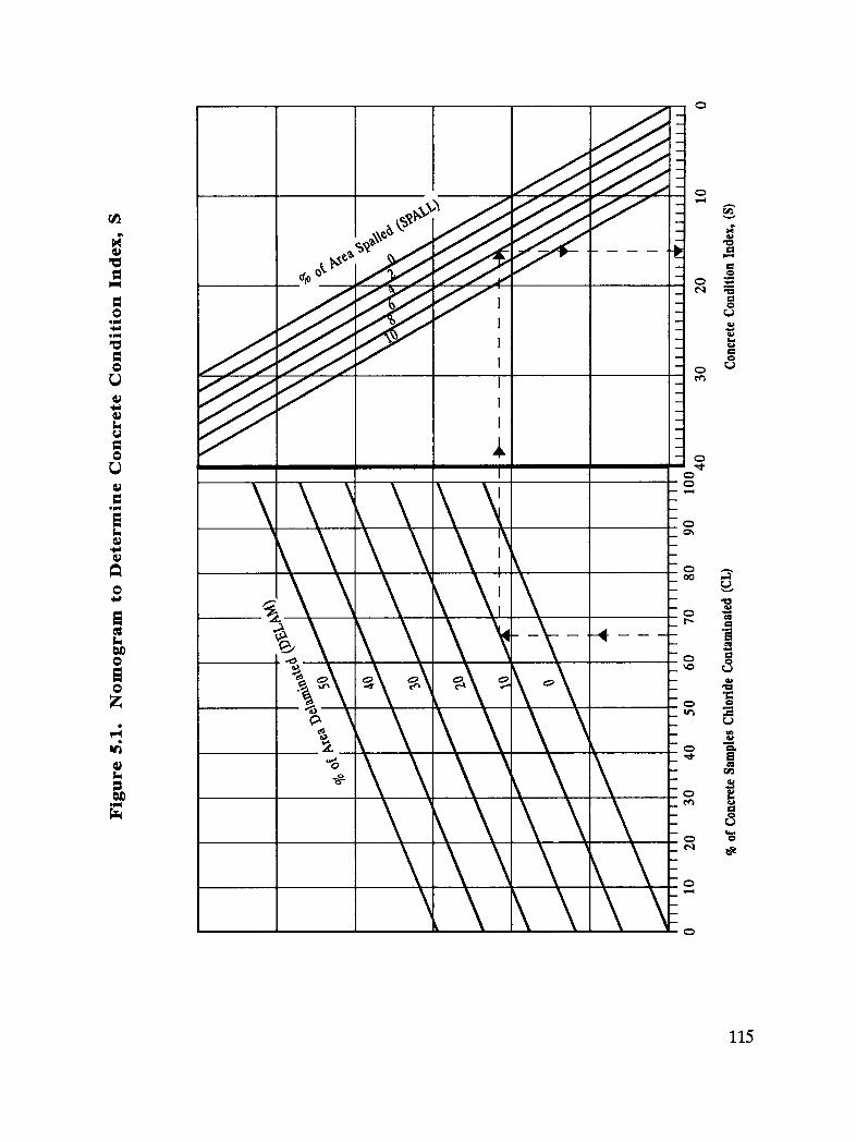
c_
60
I o _
ewq
mO_
o Z
-_---_ _
-- 0
Z _o _o
_ Zo_ _
115
6. Prediction of Performance
This chapter presents a systematic procedure for predicting the concrete condition indexat any time in the future. Site-specific concrete condition data and concrete engineeringproperties are used for this purpose.
Three cases are distinguished for the prediction of performance on the basis ofconstruction features, as follows:
1. Concrete repaired, rehabilitated, and/or protected previously.
2. Concrete not repaired, rehabilitated, and/or protected previously, andwithout a special protection built at the time of initial construction.
3. Concrete not repaired, rehabilitated, and/or protected previously, and witha special protection built at the time of initial construction.
A special protection is a positive protection against corrosion of reinforcing steel, otherthan quality conventional concrete cover. Typical concrete repair, rehabilitation, andprotection systems are presented in Chapter 8.
A predicted concrete condition index is calculated through a performance equationwhich relates the condition index to the age of concrete. The performance equationused in the methodology, which represents S-shaped curves, is given below.
S, = 100 / [1 + A exp(-Bt)] (Equation 6.1)
where
St = concrete condition index predicted for concrete age of t
A,B = constants controlling the rate of deterioration and the shapeof the curve
t = time since initial construction (age of concrete)
Parameters A and B are determined from site-specific data. One set of data (i.e.,condition index and corresponding age) relates to the present (or time of condition
117

survey, if different). The other set of data relates to the time of first sign ofdeterioration, unless the concrete was repaired, rehabilitated, and/or protected in thepast (See Section 6.1). In that case, the second set of data relates to the time of repair,rehabilitation, and/or protection.
By convention, the concrete condition index at the time of first signs of deterioration, Sd,corresponds to 15 percent chloride contamination at bar level and 0.5 percentdelamination. Thus, Sd is equal to 1.9, based on the weighting factors used in Equation5.1. The concrete age at that time, t0, is estimated from Equation 6.2, unless stateddifferently in the handbook. As an alternative to Equation 6.2, Figure 6.1 may be usedto determine t0. [Note that t0 need not be estimated as discussed, if it can be determinedfrom the concrete inspection records.]
t0 = [(2.695 d ''22t°2') / (Zt°42 p)]0.g2,s (Equation 6.2)
where
t0 = age of the concrete at time to first signs of corrosion-induceddeterioration, years
d = depth of bar cover corresponding to 10th percentile value(average depth - 1.282 standard deviation), inches.
Z t = surface chloride concentration (from 0.25 to 0.75 inches (0.6to 1.9 centimeters)) corresponding to 90th percentile value(average + 1.282 standard deviation), percent of concreteweight
t = age of the concrete when Zt is measured, years
P = concrete water-cement ratio
Figure 6.2 presents the conceptual flowchart of the overall systematic procedure todetermine parameters A and B. The following sections detail the procedure in Figure6.2 and show how to determine the parameters A and B for the three possible casesexpected in the field.
118
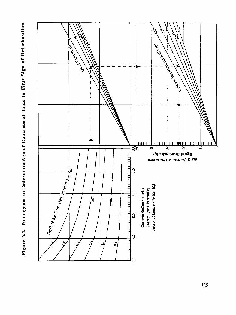
,=i
g_
oe_
omal
o I I
oma[
¢¢ I
J
[ iiii1[111 Iiiiiiiii IIIIINlvll IIIIIIIII IIIII
(Pl)uotls.ioua_a(Ijo u_!s
eml I
_ ._. -,,/ o° /
_ -
119
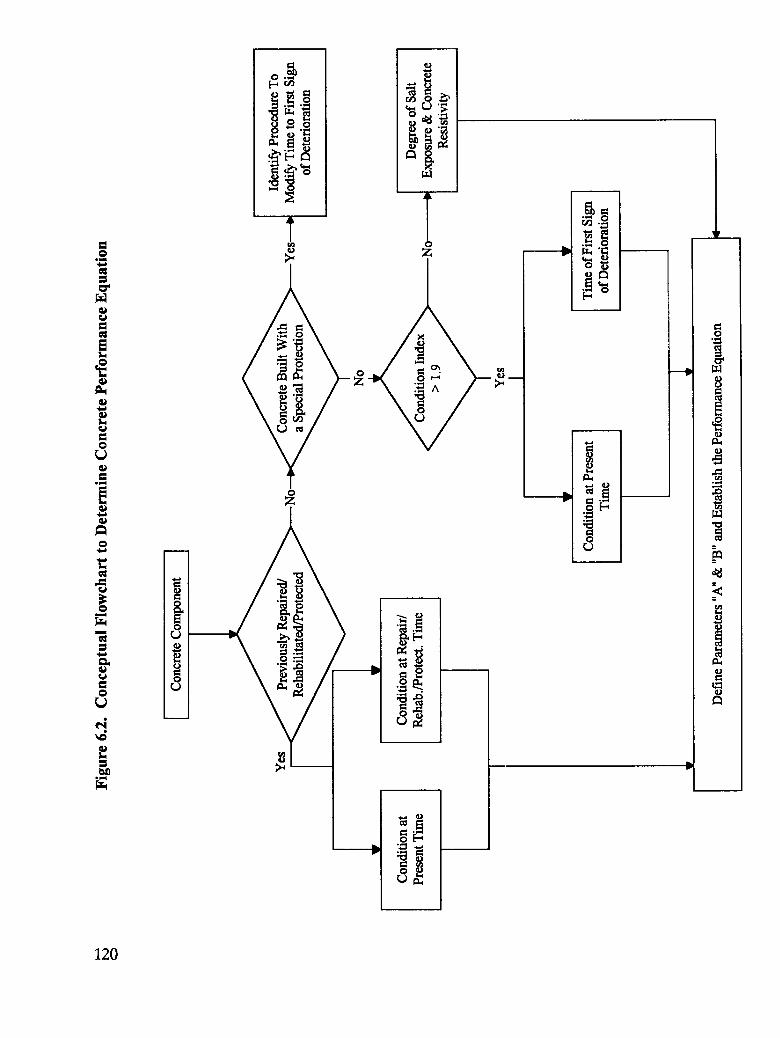
°_
_g3
L
h
120

6.1 Case 1: Concrete Repaired, Rehab'ditated and/or Protected Previously
This category applies to all concretes which were repaired, rehabilitated, and/orprotected against further corrosion-induced deterioration during their service period.
Step 1
Determine the set of data corresponding to present, as shown below.
q, = age of the concrete at present (or at time of survey, if different),years
Sp = condition index at present (or at time of survey, if different) (Equation 5.1)
Step 2
Determine the set of data corresponding to the treatment, as shown below.
tr = age of the concrete at repair, rehabilitation and/or protection, years
Sr = condition index at repair, rehabilitation and/or protection (Equation 5.1)
Note that the condition index at repair, rehabilitation and/or protection, St, relates to thecondition just after the treatment. Usually, at this stage all the deteriorated concrete hasbeen removed and replaced (if any), and the only parameter affecting the conditionindex is the level of chloride contamination.
Step 3
Use the following equations to calculate Parameters A and B.Alternatively, use Figures 6.3 and 6.4 to find B and A, respectively.
B = ln{[Sr(100 - Sp)] / [Sp(100 - S_)]} / (tr- tp) (Equation 6.3)
A = [(100 - Sp) / Sp] / [exp(-Btp)] (Equation 6.4)
121

0ell
-_'04"• "_" _ _ i',_o.%_--:a I _'#"oo_
u
II1 I ,,-
///_ _ o
II II II.
_ o _
e_
122

___ __--45.-- "__ ___2o.._ __
" 700\e '\.._ I I !<
co_o A_o_r_°_°_t_s
N
___.,_ .__ -____
g II.
123

6.2 Case 2: Concrete not Repaired, Rehabilitated, and/or Protected
Previously and without a Special Protection
This category applies to all concretes which were not repaired, rehabilitated and/orprotected against corrosion-induced deterioration during their service period, and werenot built with a special corrosion protection system at the time of their initialconstruction.
Step 1
Determine the set of data corresponding to present, as shown below.
tp = age of the concrete at present (or at time of survey, if different),years
Sp = condition index at present (or at time of survey, if different) (Equation 5.1)
If condition index Sp is
• greater than 1.9, use Steps 2 and 3;
• less than or equal to 1.9, but greater than 1.2, use Steps 4 through 6; and
• less than or equal to 1.2
- use Steps 7 through 9, if the surface chloride content (Z, Equation 6.2) is > =0.10 percent of concrete weight (4 pounds per cubic yard (2.4 kilograms percubic meter)), and
- use Steps 10 through 13 if the surface chloride content (Zt, Equation 6.2) is <0.10 percent of concrete weight (4 pounds per cubic yard (2.4 kilograms percubic meter)).
Step 2
Determine the set of data corresponding to the first signs of deterioration, as shownbelow.
td = age of the concrete at time to first deterioration, years (Equation 6.2or Figure 6.1)
Sd = condition index at time to first deterioration, 1.9
124
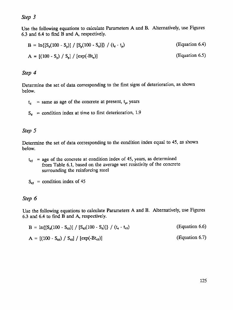
Step 3
Use the following equations to calculate Parameters A and B. Alternatively, use Figures6.3 and 6.4 to find B and A, respectively.
B = ln{[Sd(100 - Sp)] / [Sp(100 - Sd)]} / (td- tp) (Equation 6.4)
A = [(100 - Sp) / Sp] / [exp(-Btv)] (Equation 6.5)
Step 4
Determine the set of data corresponding to the first signs of deterioration, as shownbelow.
ta = same as age of the concrete at present, tp, years
Sd = condition index at time to first deterioration, 1.9
Step 5
Determine the set of data corresponding to the condition index equal to 45, as shownbelow.
t45 = age of the concrete at condition index of 45, years, as determinedfrom Table 6.1, based on the average wet resistivity of the concretesurrounding the reinforcing steel
$45 = condition index of 45
Step 6
Use the following equations to calculate Parameters A and B. Alternatively, use Figures6.3 and 6.4 to find B and A, respectively.
B = In{[Sd(100 - 845)] / [545(100 - Sd)]} / (td- t45) (Equation 6.6)
A = [(100 - $45) / $45]/ [exp(-Bt45)] (Equation 6.7)
125

Step 7
Determine the set of data corresponding to the first signs of deterioration, as shownbelow.
td = age of the concrete at time to first deterioration, years (Equation 6.2,or Figure 6.1)
Sd = condition index at time to first deterioration, 1.9
Step 8
Determine the set of data corresponding to the condition index equal to 45, as shownbelow.
h5 = age of the concrete at condition index of 45, years, determined fromTable 6.1 based on the average wet resistivity of the concretesurrounding the reinforcing steel
$45 = condition index of 45
Step 9
Use Equations 6.6 and 6.7 or Figures 6.3 and 6.4 to find parameters B and A,respectively (see Step 6).
Step 10
Estimate the surface chloride levels in 10 years, based on the level of snowfall and/orexposure to marine environment, as shown in Table 6.2.
Step 11
Determine the set of data corresponding to the first sign of deterioration, using theestimate of surface chloride content in 10 years, as shown below.
td = age of the concrete at time to first deterioration, years (Equation 6.2,or Figure 6.1)
Sd = condition index at time to first deterioration, 1.9
126

Table 6.1. Correlation of Rate of Deterioration and Resistivity
Average Wet Resistivity Years to Index of 45ohm-em (t,_)
Less than 7,500 td + 10
7,500 to 30,000 t d -I- 20
Higher than 30,000 td + 35
Table 6.2. Estimates of Surface-Level Chloride Content in 10 Years
Snowfall Range, inch I Marine Exposure 1and Distance Future Surface Chlorides 2 (in 10from Seawater years) Whichever is Greater
0to3 NO Z, (t+ 10)/tor0.04 percent of concrete weight
3to12 NO Zt (t+10) /tot0.10 percent of concrete weight
0to12 YES > 25ft Zt (t + 10)/tor0.10 percent of concrete weight
0to 12 YES < 25 ft Zt (t + 10)/tor0.25 percent of concrete weight
> 12 NO Z, (t + 10)/tor0.25 percent of concrete weight
> 12 YES > 25ft Zt (t + 10)/tor0.35 percent of concrete weight
> 12 YES < 25ft Zt (t + 10)/tor0.45 percent of concrete weight
1: One inch is 2.54 centimeters, and one foot is 0.305 meters.
2: "Zt" is the surface chloride content, percent of concrete weight (divide by 0.025 to convert to pounds percubic yard, or divide by 0.042 to convert to kilograms per cubic meter), as defined in Equation 6.2. "t" isthe duration of exposure when 7_ is measured, years.
127

Step 12
Determine the set of data corresponding to the condition index equal to 45, as shownbelow.
tas = age of the concrete at condition index of 45, years, determined fromTable 6.1 based on the average wet resistivity of the concretesurrounding the reinforcing steel
$45 = condition index of 45
Step 13
Use Equations 6.6 and 6.7, or Figures 6.3 and 6.4, to find parameters B and A,respectively (see Step 6).
6.3 Case 3: Concrete not Repaired, Rehabilitated and/or ProtectedPreviously, and with a Special Protection Built at the Time of InitialConstruction
This category applies to all concretes which .were not repaired, rehabilitated and/orprotected against corrosion-induced deterioration during their service period, and werebuilt with a special corrosion protection system at the time of their initial construction.
Follow all the steps described in Case 2, Concrete without a Special Protection, to findthe performance equation. However, tdtime tO first sign of deterioration, should bemodified where Equation 6.2 (or Figure 6.1) is used, based on the type of protectivesystem. The following sections present the types of protective systems and procedures tomodify td for those systems.
Concrete Overlays:
• Conventional Concrete
• Low-Slump Dense Concrete
• Silica Fume Concrete
• Latex-Modified Concrete
128

Determine a weighted average water-cement ratio, as shown below, based on thethickness of the overlay and the bar cover depth (excluding the overlay). Input theweighted average water-cement ratio and the total bar cover depth (including theoverlay) in Equation 6.2 (or Figure 6.1), and find the modified h.
Weighted Average W-C Ratio =
[(Overlay Representative W-C Ratio from Concrete Permeability, AASHTOT277) x (Overlay Thickness) + (Total Cover - Overlay Thickness) x (BaseConcrete W-C Ratio)] / [Total Cover] (Equation 6.8)
Membranes, Sealers, Coatings
• Membrane with Asphalt Concrete Overlay
• Penetrating Sealer
• Surface Coating
Determine the number of years the protective system will block the chlorides frompenetrating the concrete (effective service life of the protective system), and add it to thenumber of years found from Equation 6.2 (or Figure 6.1); use the result as the modifiedtd.
The effectiveness of membrane and sealer protective system may be checked by testmethods described in Cady and Gannon 3.
Concrete Admixtures
• Concrete with Corrosion Inhibitor
• Concrete with Silica Fume
For corrosion inhibitors, determine the number of years the protective system will delayinitiation of the corrosion-induced deterioration, based on the amount of inhibitor addedto the concrete mix. Add the number of years found to the number of years obtainedfrom Equation 6.2 (or Figure 6.1); use the result as the modified h.
For concrete with silica fume admixture, determine a representative water-cement ratiofrom the concrete permeability value (AASHTO T277) and resistivity value. Input therepresentative water-cement ratio and the actual bar cover depth in Equation 6.2 (orFigure 6.1), and find the modified h.
129

Coated Reinforcing Steel
• Epoxy-Coated bar
• Galvanized bar
Estimate the number of years to initiation of concrete deterioration with coated bars,and number of years to initiation of concrete deterioration if the bars were not coated.Use the same bar cover depth and water-cement ratio for both cases. Find thedifference between the two, and add the difference to the number of years obtained fromEquation 6.2 (or Figure 6.1), and use the result as the modified t0.
130
7. Evaluation of Performance
Chapter 6 established a performance equation relating the concrete condition to the ageof the concrete. This chapter will assist the user understand deterioration of theconcrete by illustrating the equation graphically. Use Figure 7.1 to identify the concreteperformance curve based on the value of Parameters A and B determined in Chapter 6.For previously repaired, rehabilitated, and/or protected concretes (Case 1, Chapter 6),only consider the portion of the curve beyond the concrete age at repair, rehabilitation,and/or protection, tr.
As a concrete bridge component ages, its condition gradually deteriorates and itscondition index increases to a point that some type of treatment must be done. Asdiscussed in Chapter 5, the user should determine the maximum tolerable conditionindex, Sin,based on the structural features of the component and/or the ride quality ofthe deck. The period of time between the present time and time corresponding to Smisthe "treatment consideration period." This is expressed in the following equation.
Treatment Consideration Period = tm- tp (Equation 7.1)
where
t_ = age of concrete when condition index is Sin,determined from thefollowing equation or the performance curve (Figure 7.1), years
tm = -{In[(100 - Sin)/ (A Sm)]}/ B (Equation 7.2)
ta, = age of concrete at present, years
The rest of this manual should be used to determine the timing of the treatment withinthe "treatment consideration period," as well as the type of the treatment, for maximumcost-effectiveness.
131

Figure 7.1. Concrete Performance Curves, B-- 0.10
100
9O
8O
7O
60v
M
50
q_
40
30
20
10
00 10 20 30 40 50 60 70
ConcreteAge,Years(t)
132

Figure 7.1. (Continued) Concrete Performance Curves, B=.12
100
9O
8O
7O
6Ov
5o.2
"_ 400
30
2O
10
00 i0 20 30 40 50 60 70
ConcreteAge,Years(t)
133

Figure 7.1. (Continued) Concrete Performance Curves, B=.14
100
90
8O
70
60
5O
.=.40
O
30
20
10
00 10 20 30 40 50 60 70
ConcreteAge,Years(t)
134

Figure 7.1. (Continued) Concrete Performance Curves, B=.16
100
90
80
70
60
"_ 50ae_o
q_= 40O
30
20
i0
00 I0 20 30 40 50 60 70
ConcreteAge,Years(t)
135
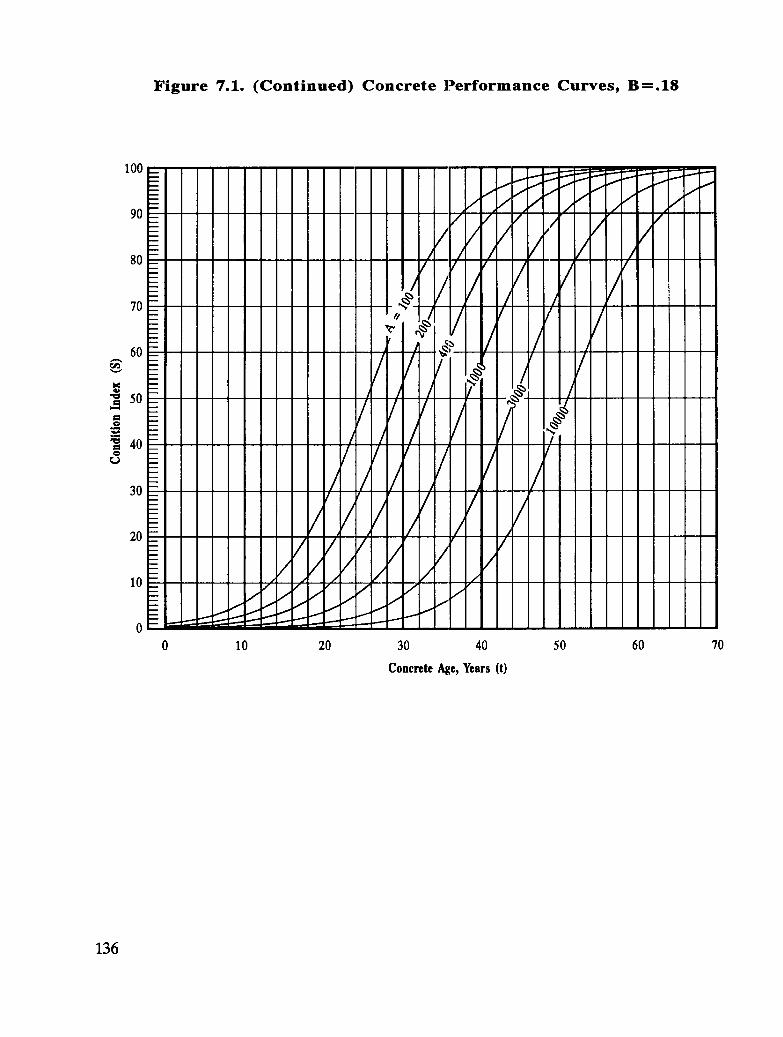
Figure 7.1. (Continued) Concrete Performance Curves, B--.18
100
9O
8O
7O
6O
"_ 50
40eso
3O
2O
I0
00 I0 20 30 40 50 60 70
ConcreteAge,Years(t)
136
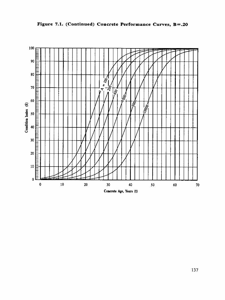
Figure 7.1. (Continued) Concrete Performance Curves, B=.20
100
9O
8O
7O
6OC_
"_ 5O
N- 40O
30
2O
10
0
0 10 20 30 40 50 60 70
ConcreteAge,Years(t)
137

Figure 7.1. (Continued) Concrete Performance Curves, B=.25
100
9O
8O
7O
6O
50e_
"_ 4OO
30
2O
10
O0 10 20 30 40 50 60 70
ConcreteAge,Years(t)
138
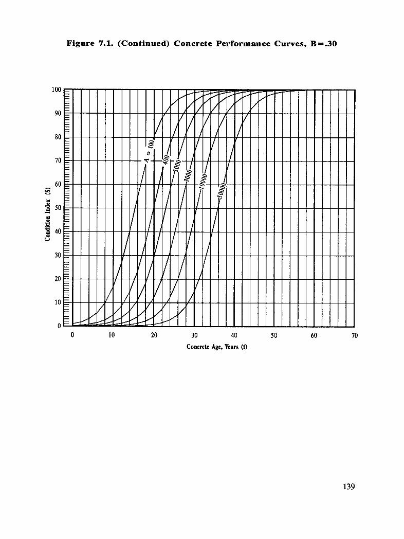
Figure 7.1. (Continued) Concrete Performance Curves, B=.30
100
9O
80
7O
60v
"_ 50es
"_ 40eso
3O
2O
I0
0
0 I0 20 30 40 50 60 70
ConcreteAge,Years(t)
139
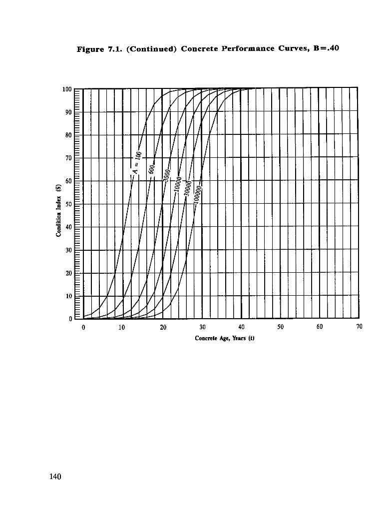
Figure 7.1. (Continued) Concrete Performance Curves, B--.40
100
9O
8O
7O
6OrJ_
"_ 50
.o
"_ 40O
30
2O
10
00 10 20 30 40 50 60 70
ConcreteAge,Years(t)
140
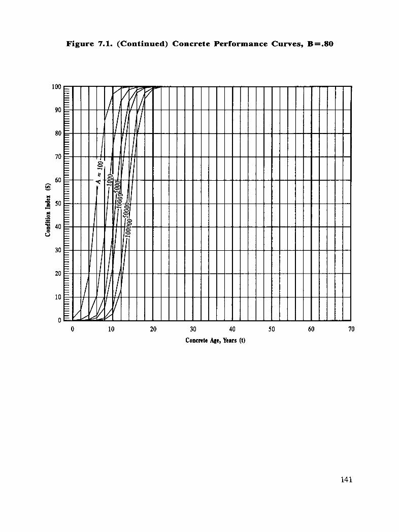
Figure 7.1. (Continued) Concrete Performance Curves, B----.80
100 _- _ _ 7- ;i-" i ! ,
- It _90 _ f I
80 - / ,
70_
60-
_ =•_ 5o-
"_ 40-O
3o-
20- _
1o-/ !'/z
0 --
O lO 20 30 40 50 60 70
ConenteAge,Years(t)
141

8. Compatible Treatment Alternatives
The following sections identify a range of treatment alternatives from which the selectioncan be made. Generally, there are two types of treatment, deck treatment and structuraltreatment. Structural treatment, as defined here, applies only to superstructure andsubstructure elements (i.e., non-deck elements). A comprehensive description ofconcrete treatment alternatives is provided in SHRP research by Weyers et al.4
8.1 Deck Repair
Concrete Patches, Chloride Contaminated Concrete Left in Place
In this procedures deteriorated concrete is removed to the depth required and replacedwith concrete.
• Conventional Concrete Patches
• Quick-Set Hydraulic Concrete Patches
• Polymer Concrete Patches
82 Deck Rehabilitation/Protection
Concrete Patches, Chloride-Contaminated Concrete Removed
In this procedure, deteriorated and contaminated concrete are removed to the depthrequired and replaced with concrete.
• Conventional Concrete Patches
• Quick-Set Hydraulic Concrete Patches
• Polymer Concrete Patches
143
Corrosion Inhibitor Application
• Corrosion Inhibitor Application
Concrete Overlays
• Conventional Concrete
• Low-Slump Dense Concrete
• Silica Fume Concrete
• Latex-Modified Concrete
• Polymer Concrete
Asphalt Concrete and Waterproofing Membrane Overlays
• Preformed Membrane
• Applied-in-Place Membrane
Sealers and Coatings
• Sealers and Coatings
Cathodic Protection
• Slotted System without Overlay
• Overlaid System
8.3 Structural Repair
Concrete Replacement, Chloride Contaminated Concrete Left in Place
In this procedure, deteriorated concrete is removed to the depth required and replacedwith concrete.
144
• Recasting with Concrete (formwork required)
• Preplacing Dry Aggregate and Grouting (formwork required)
• Spraying-on Concrete (Shotcrete)
• Patching with Trowel-Applied Mortar
- Conventional Mortar
- Quick-Set Hydraulic Mortar
- Polymer Mortar
8.4 Structural Rehabilitation/Protection
Concrete Replacement, Chloride-Contaminated Concrete Removed
In this procedure, deteriorated and contaminated concrete are removed to the depthrequired and replaced with concrete.
• Recasting with Concrete (formwork required)
• Preplacing Dry Aggregate and Grouting (formwork required)
• Spraying-on Concrete (Shotcrete)
• Patching with Trowel-Applied Mortar
Conventional Mortar
Quick-Set Hydraulic Mortar
Polymer Mortar
Concrete "Covers"
• Spraying-on Concrete (Shotcrete)
• Concrete Jacketing (formwork required)
145
Sealers and Coatings
• Sealers and Coatings
Cathodic Protection
• Cathodic Protection
8.5 Compatible Treatments
Prior to considering all of the alternatives listed in this chapter for a specific site, theuser should be aware that restrictions may prevent certain alternatives at that site.Tables 8.1 and 8.2 should be consulted for deck treatment and structural treatment,respectively, to screen out those treatment alternatives which are not compatible with theconcrete because of their technical disadvantages.
146

Table 8.1. Selection of Compatible Deck Treatment Alternatives
Technical Conc. AC Seal. Cathod. Reason
Disadvantage Over. Memb. Coat. Protect.
Additional dead load Not Not Not Overlays add to dead load2.critical Good Good Good I
Active cracks in cone. Not Not Active cracks reflect throughGood Good 3 concrete.
Existing overlay on Not Not4 Removal of old system resultsdeck Good Good in rough surface5.
Concrete surface Not Rough concrete surfacesealed Good
Existing slotted Not Scarifying concrete damagescathod, protect. Good anodes
Existing polymer Not Good Insulated barsinjection repair inconcrete
Electricity not Not Cathodic protection needsavailable Good electricity
Skid resistance Not Skid resistance may decreasecritical Good6
Steep grades and/or Not Concrete may flow after strikecrossfalls Good7 off
Sharp skew and/or Not Difficult to pave with concretecurvature Good finishing machines
1. When cathodic protection is used with an overlay.2. Unless, an existing overlay (or a layer of the concrete) is removed and replaced.3. When cathodic protection is used with a concrete overlay.4. May be applied on some concrete overlays.5. Rough concrete surface can puncture membranes, unless a smooth concrete surface can be provided
for the new membrane.
6. Exceptions can exist.7. when slump is 4.5 inches (11.4 centimeters) or more.
147
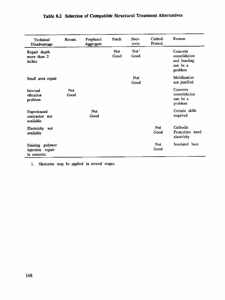
Table 8.2 Selection of Compatible Structural Treatment Alternatives
Technical Recast. Preplaced Patch Shot- Cathod. Reason
Disadvantage Aggregate crete Protect.
Repair depth Not Not' Concretemore than 2 Good Good consolidation
inches and bondingcan be a
problem
Small area repair Not MobilizationGood not justified
Internal Not Concretevibration Good consolidation
problem can be aproblem
Experienced Not Certain skillscontractor not Good requiredavailable
Electricity not Not Cathodicavailable Good Protection need
electricity
Existing polymer Not Insulated barsinjection repair Goodin concrete
1. Shotcrete may be applied in several stages.
148

9. Cost Items Associated withTreatment (Agency Costs)
Costs associated with various treatments should be known in order to select the most
cost-effective alternative and determine its timing. Costs can vary significantly from onearea to another and from time to time, depending on many factors. The user generallyhas the most reliable information regarding the cost of a certain treatment in a givenjurisdiction.
However, before the user arrives at any cost for a treatment, the standard cost itemsassociated with that treatment must be identified. This chapter of the handbookprovides standard highway agency cost items associated with each treatment included inthe handbook (Chapter 8). User cost items are discussed in Chapter 10.
The user should determine the cost of each item separately for the treatment consideredand then total those itemized costs. Users with no previous experience with the cost ofthe items outlined in this chapter may consult SHRP research by Weyers et al. 4 and byBennett, et al.5
The user may of course, change treatment procedures outlined here to suit agencypolicies and practices.
9.1 Cost Items Associated with Applying Deck Treatments
Concrete Patches
Cost items in this category are as follows:
• Removing contaminated and/or deteriorated concrete.
• Patching with concrete and curing.
• Traffic control, when bridge is partially open to traffic.
149

Cost items in this category should be expressed in terms of dollars per cubic yard ofpatches, or dollars per square foot of patches, if the:depth of the patch is taken intoconsideration.
Corrosion Inhibitor Application
Cost items in this category are as follows:
• Applying corrosion inhibitor.
- When there is not an existing overlay; spray the inhibitor to soakinto the concrete.
- When there is an existing overlay; this treatment may not beconsidered.
• Traffic control, when the bridge is partially open to traffic.
Cost items in this category should be expressed in terms of dollars per square foot ofdeck area.
Concrete Overlays
Cost items in this category are as follows:
• Surface preparation.
- When there is not an existing overlay; scarify the concrete surface(sand- or shotblasting for polymer concrete).
- When there is an existing overlay; remove the existing overlay.
• Placing and curing concrete.
• Traffic control, when the bridge is partially open to traffic.
Cost items in this category should be expressed in terms of dlollars per square foot ofdeck area.
150

Asphalt Concrete and Waterproofing Membrane Overlays
Cost items in this category are as follows:
• Surface preparation.
When there is not an existing overlay; sandblast the concrete surface.
When there is an existing overlay; this treatment may not be viable,since removing the existing overlay will result in a rough surface (seeTable 8.1 for further information).
• Placing membrane.
• Placing asphalt concrete.
• Traffic control, when the bridge is partially open to traffic.
Cost items in this category should be expressed in terms of dollars per square foot ofdeck area.
Sealers and Coatings
Cost items in this category are as follows:
• Surface preparation.
- When there is not an existing overlay; sandblast the concrete surface.
- When there is an existing overlay; this treatment may not be used,since sealers are generally not applied on special concrete overlays oron asphalt concrete surfaces; if the existing overlay is removed, it willresult in a rough surface (see Table 8.1 for further information).
• Applying sealer or coating.
• Traffic control, when the bridge is partially open to traffic.
Cost items in this category should be expressed in terms of dollars per square foot ofdeck area.
151

Cathodic Protection, Slotted System
Cost items in this category are as follows:
• Surface preparation.
- When there is a concrete surface; saw cut slots.
- When there is an existing di-electric overlay (e.g., asphaltconcrete/membrane, or polymer concrete); this treatment is notrecommended, since removing the existing overlay will result in arough surface.
• Placing wire anodes in slots.
Placing electrically conductive polymer in slots.
Traffic control, when the bridge is partially open to traffic.
Cost items in this category should be expressed in terms of dollars per square foot ofdeck area.
Cathodic Protection, Overlaid System
Cost items in this category are as follows:
• Surface preparation.
- When there is not an existing overlay; Scarify the concrete surface.
- When there is an existing overlay; remove the existing overlay.
• Attaching of mesh anodes to the surface.
• Placing, and curing concrete overlay.
• Traffic control, when the bridge is partially open to traffic.
Cost items in this category should be expressed in terms of dollars per square foot ofdeck area.
152

9.2 Cost Items Assodated with Applying Structural Treatments
Concrete Replacement
Cost items in this category are as follows:
• Removing contaminated and/or deteriorated concrete.
• Formwork (formwork is not required for shotcrete and patching)
• Placing and curing concrete.
• Traffic control, when the bridge is partially open to traffic.
Cost items in this category should be expressed in terms of dollars per cubic yard ofreplacement, or dollars per square foot of replacement, if the depth of the patch is takeninto consideration.
Concrete "Covers"
Cost items in this category are as follows:
• Surface preparation (sandblasting).
• Formwork (form work is not required for shotcrete)
• Placing and curing concrete.
• Traffic control, when the bridge is partially open to traffic.
Cost items in this category should be expressed in terms of dollars per square feet ofconcrete area treated.
Sealers and Coatings
Cost items in this category are as follows:
• Surface preparation (sandblasting).
• Applying sealer or coating.
• Traffic control, when bridge is partially open to traffic.
153
Cost items in this category should be expressed in terms of dollars per square foot ofconcrete area treated.
Cathodic Protection
Cost items in this category are as follows:
• Surface preparation (sandblasting).
• Attaching mesh anodes to the surface.
• Placing and curing protective mortar (shotcrete).
• Traffic control, when the bridge is partially open to traffic.
Cost items in this category should be expressed in terms of clollars per square foot ofconcrete area treated.
9.3 Cost Item Associated with Monitoring and Maintaining Treatment
Certain treatments may require periodic costs of monitoring and/or maintaining thetreatment. For example, cathodic protection installations need to be periodicallymonitored for the polarized steel potentials, regardless of the age of the system, tomaintain the potentials within the prescribed limits.
154

10. Cost Items Associated withTreatment (User Costs)
Two types of user costs are included in the methodology. Those are: (1) during-treatmentcosts, and (2) prior-to-treatment costs.
10.1 During-Treatment Costs
Costs during the treatment are related to increases in travel time caused by trafficcongestion on the bridge, or by a detour around the bridge during bridge closure. Usethe equation given below, or Figure 10.1, to find the user costs resulting from the degreeof bridge closure.
U1 = KI t_to qo (Equation 10.1)
where:
U1 = user costs during the treatment period, dollars
K1 = value of bridge user time while traveling, dollars per minute per vehicle
to = duration of treatment, days
qo = average two-way daily traffic volume across the bridge, vehicles per day
tt = increment in travel time across the bridge (or in detour around the bridge)caused by construction, minutes
For traveling across the bridge, tt may be obtained from Equation10.2 or Figure 10.2.
t_ = 0.15 tf [(qo / C1)4- (qo / C)'] (Equation 10.2)
where
tf = free-flow travel time across the bridge, minutes
155

C1 = two-way capacity of the brJ[dgeduring construction, vehiclesper day
C = two-way capacity of the brJidge during normal periods, vehiclesper day
10.2 Prior-to-Treatment Costs (Decks Only)
Costs in the period prior to treatment are a function of the condition of the bridge deckand its effect on traffic flow. A badly spalled deck would impede traffic flow, causingspeed reductions, congestion, and resulting increase in travel time and cost. Use thefollowing equation, or Figure 10.3, to find user costs due to worsening deck condition fora given year.
U2 = K2 [S / Sin]4 [ 365 qo] (Equation 10.3)
where
U2 = user costs due to worsening deck condition, dollars per year
K2 = a calibrating constant, dollars per vehicle
[K2 = a tf KI : See "During-Treatment Costs" for definitions of K 1
and tf. Parameter "a" is the percentage of free-flow travel time, tf,representing the increment in travel time when S = Sm.]
S = concrete condition index for the year considered (Chapter 6)
S m = maximum tolerable condition index (Chapter 5)
qo = average two-way daily traffic volume across the bridge, vehicles per day
156

5000 , _
__"_ ._ ---
= _,el _--,
0 I m
°° 'a ''
== "oooX\ _.
157

_ jN _
- 0
gZ _
0
°00
158
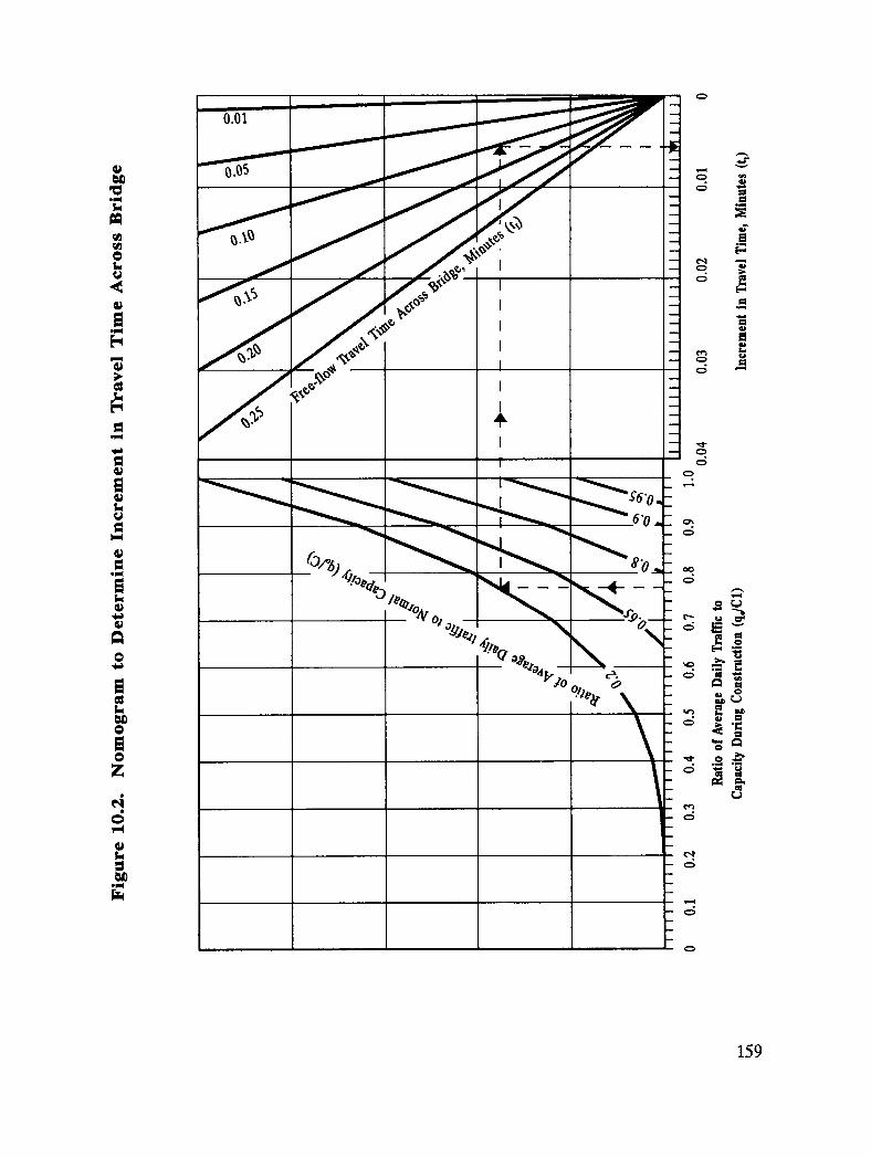
0.01
- i0.q35
_.//_,__, _/._, ,. -
°" I -
.
_'_ I "¢,._. --
]°°/_e_ _ -- ._.
o- r,_
_ -
" EN e,_
159

Figure 10.3. Nomogram to DeterminE: User Costs Prior to Treatment
2Om
./
0
0.2 0.3 0.4 0.5 0.6 0.7 0.8 0.9 1.0
Ratio of Condition Index to
MaximumCondition Index (SIS.)
160

II. Decomposing ConcreteCondition Index
In order to estimate agency costs and user costs associated with a treatment (Chapter 9,and 10), the amount of concrete repair (removing and replacing deteriorated andpossibly contaminated concrete) needs to be predicted at the time of treatment. Theuser can predict the amount of deterioration and contamination in the future bydecomposing the future concrete condition index, S, into its component parts (i.e., CL,DELAM, and SPALL, see Chapter 5). Use the following procedure to decomposeconcrete condition index.
11.1 Assumptions
1. Chloride contamination, CL, increases 5 percent for each index increase of oneunit.
2. For all deck concrete except those with 1-inch (2.54 centimeters), or thicker,concrete overlays: DELAM is 4 times SPALL. For all deck concrete with 1-inch or thicker, bonded concrete overlays: DELAM is 8 times SPALL.
3. For all non-deck concrete except those with 1-inch (2.54 centimeters), orthicker, concrete jackets or shotcrete: DELAM is 8 times SPALL. For all non-deck concrete with 1-inch (2.54 centimeters), or thicker, concrete jackets orshotcrete: DELAM is 16 times SPALL.
11.2 Procedure (valid only for weighting factors used in Equation 5.1)
CL = 5 S and CL < = 100 (Equation 11.1)
DELAM = (8.5 S- CL) / (2.5 + 7.5/N) (Equation 11.2)
where
N = ratio of DELAM to SPALL, as discussed in the assumptions
SPALL = DELAM / N (DELAM does not include SPALL) (Equation 11.3)
161

12. Prediction of Performance,Treated Concrete
The methodology employs life-cycle cost analysis to determine the cost-effectiveness of aproposed treatment. Therefore, the service life of the treated concrete also needs to bepredicted. The aim of this chapter is to predict the effective service life expected of thetreated concrete. As defined in this chapter, at the end of the effective service life of thetreated concrete the concrete condition index is the maximum tolerable, SIn. Use the
following procedures to predict the effective service life of the treated concrete. Applythe same effective service life to the next cycles of treatment.
[It should be noted that in order to achieve the effective service life predicted for thetreated concrete in this chapter, the treatment may be repeated, depending on thedurability of the treatment itself. This may include reapplying sealers/coatings, removingand replacing overlays, and renewing cathodic protection systems. The user shoulddetermine the service life expected of the treatment itself, on the basis of environmentalfactors. SHRP research by Weyers et al.4 may be consulted for this purpose.]
12.1 Case 1: Concrete not Repaired, Rehabilitated, and/or ProtectedPreviously
Case 1 applies to all concretes which will be repaired, rehabilitated, and/or protected forthe first time.
Two factors affect the effective service life of the concrete after the treatment. Those
are (1) the inherent corrosion mechanism active at the time of treatment, and 2) thetreatment's effect on the future corrosion process. Generally, there are five trends in thecorrosion process after the treatment, as shown in Figure 12.1 and described below.
1. The rate of corrosion continues to increase at the same rate after the
treatment. This condition is represented by K = i in Figure 12.1 (typicalof only patching when deteriorated concrete is removed and replaced, butcontaminated concrete is left in place). Estimate the effective service lifeof the treated concrete from Equation 12.1 (see Figure 12.1 for derivationof the equation; note that K = 1), or Figure 12.2.
163

Figure 12.1. Trends of Corrosion Proces.,l After Treatment
-1/3<K<0
II
to t*
Corrosion Rehabilitation/Protection
Starts Applied
ConcreteAge
K = Ratio of Slope of Corrosion Rate Line After Treatmentto
Slope of Corrosion Rate Line Before Treatment.
164
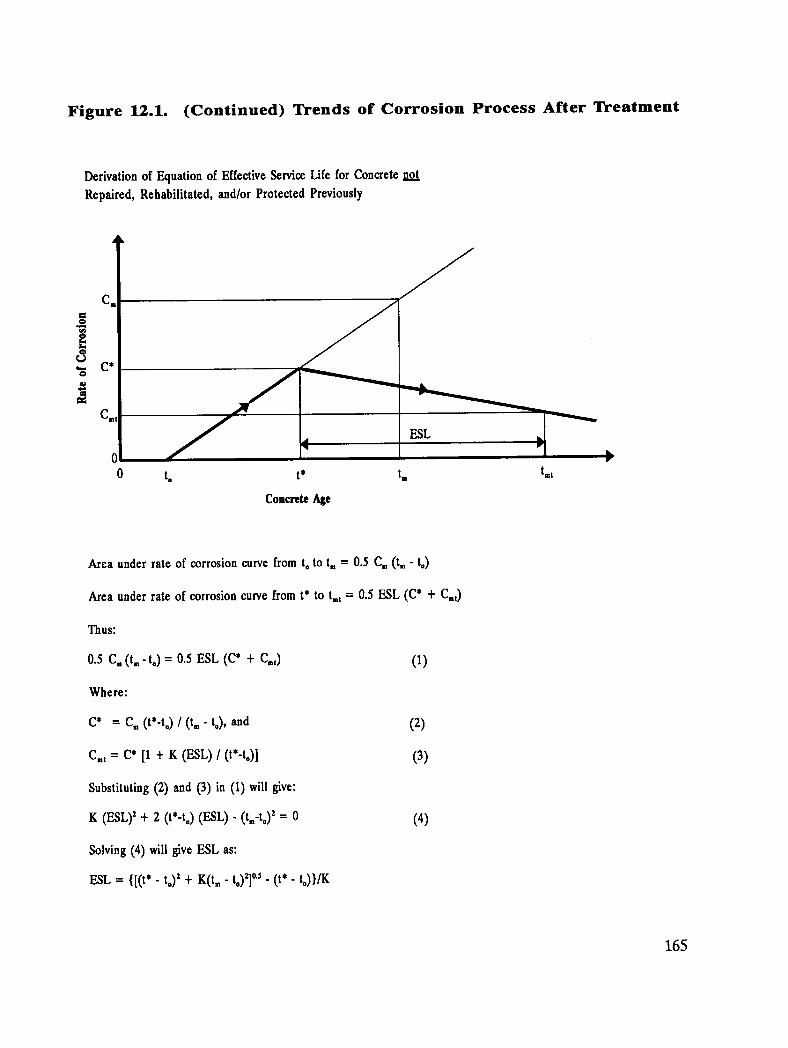
Figure 12.1. (Continued) Trends of Corrosion Process After Treatment
Derivation of Equation of Effective Service Life for Concrete not
Repaired, Rehabilitated, and/or Protected Previously
Area under rate of corrosion curve from toto t. = 0.5 C. (t. - to)
Area under rate of corrosion curve from t* to t.t = 0.5 ESL (C* + C.t)
Thus:
0.5 C. (t.-to) = 0.5 ESL (C* + C,_,) (1)
Where:
C* = C. (t*-to)[ (t.- to), and (2)
C., = C*[1 + K (ESL)/ (t*-to)] (3)
Substituting (2) and (3) in (1) will give:
K (ESL)2 + 2 (t*-to) (ESL) - (t.-t,) 2 = 0 (4)
Solving (4) will give ESL as:
ESL = {[(t* - t,)2 + K(t.-t,)2] °5- (t*-to)}/K
165
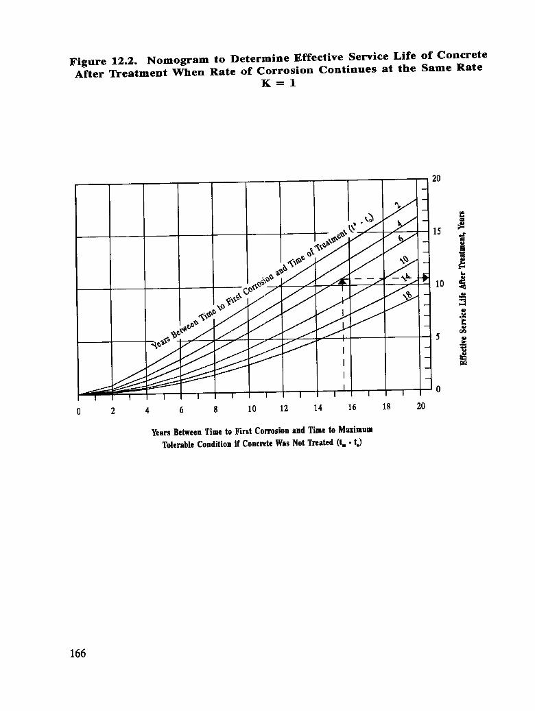
Figure 12.2. Nomogram to Determine Effective Service Life of ConcreteAfter Treatment When Rate of Corrosion Continues at the Same Rate
K---1
2O
0 2 4 6 8 10 12 14 16 18 20
YearsBetweenTimeto First CorrosionandTimeto M_'_imnm
TolerableConditionif ConcreteWasNot Treated(t. - t.)
166
ESL = [(t'- to)2 + (t=- to)2]°'s- (t'- to) (Equation 12.1)
where
ESL = effective service life, years
t* = age of concrete at time of treatment, years
t_ = age of concrete at condition index of S=, if the concrete wasnot treated (Chapter 7), years
to = age of concrete at time to first sign of corrosion, years (Find td,time tO first sign of deterioration from Chapter 6. Enter Figure12.3 with tdand determine to.)
2. The rate of corrosion increases gradually after the treatment, but at aslower rate. This condition is represented by 0<K< 1/3 in Figure 12.1(typical of sealers, coatings, and asphalt concrete/membrane systems).Estimate the effective service life of the treated concrete from Equation12.2 (see Figure 12.1 for derivation of the equation), or Figure 12.4.
ESL = {[(t*- to)2 + K(1G-to)2]°s- (t'- to) } / K (Equation 12.2)
where
K = the ratio of the slope of corrosion rate increase after treatmentto the slope of corrosion rate increase before treatment(0 <I,:< 1/3).
See 1., above, for the definition of the other parameters in Equation12.2.
3. The rate of corrosion levels off after the treatment. This condition is representedby K = 0 in Figure 12.1 (typical of asphalt concrete/membrane systems, sealers,and coatings at their best performance; or concrete overlays at their worstperformance). Estimate the effective service life of the treated concrete fromEquation 12.3 (see Figure 12.1 for derivation of the equation; note that K = 0),or Figure 12.5.
ESL = 0.5 (t=- to)2/(t °- to) (Equation 12.3)
167

Figure 12.3. Chart to Find Age of Concrete at Time of First Corrosion
50
J40 "_
- d"
j _ 30O
j - 20
O
f I - 10/ I =
I
I I I I I I I I I I I I ! I I I I Ill I I I I I I I I I I I I I I I I I 0
5 i0 15 20 25 30 35 40 45 50
ConcreteAgeatFirstDeterioration,Years(t_)
168
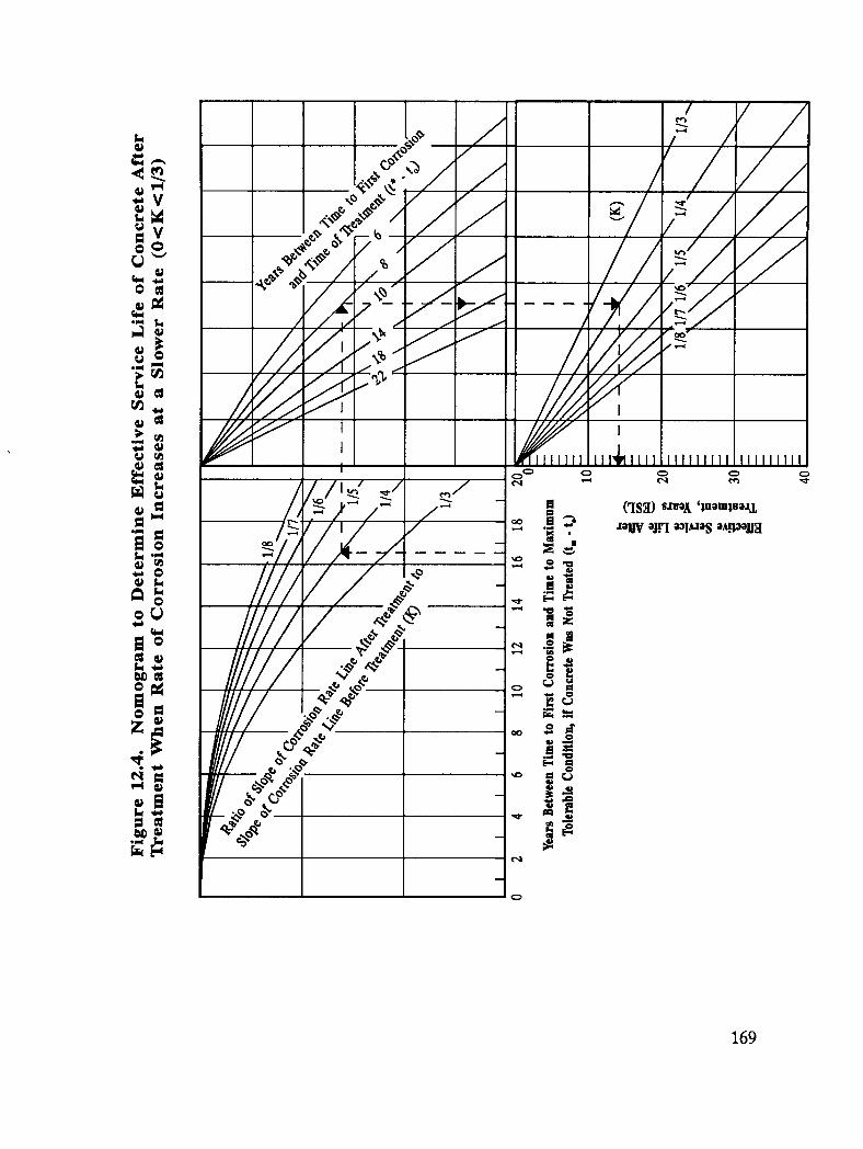
, Loo.4 _ ///• .,# /"J I_ ,,c,o,,_ / / /
-_ --o_,--°°d//I _/,-_/'//
_ /,.'k'.a'.:?_" I ///P'_ /
_ _ IIIIIIII L
_'_"_ 111/1// L¢ 4 .!i
////// I .,_°oe /o 8 __" IIIII/I ...*'_.°" J _IIIII/ "_ ,@'_ 1- ___8
IIII I 0 __ I 0- =Nil I _%, _- -I ._ ;_
_** llll l _ _ I l,_ m
169

Figure 12.5. Nomogram to Determine Effective :Service Life ofConcrete After Treatment When Rate of Corrosion Levels Off
(K = O)
] ,_ /_ 50@_ / 40
///+; ,/ J/..'_o_.a
_¢_____,_-____ '_-0 2 4 6 8 10 12 14 16 18 20
YearsBetweenTimeTo FirstCorrosionandTimeto Maximum
TolerableConditionif ConcreteWasNot Treated(t=- t.)
170
See 1., above, for the definition of the parameters in Equation 12.3.
4. The rate of corrosion decreases gradually after the treatment. Thiscondition is represented by -1/3 <K< 0 (typical of concrete overlays).Estimate the effective service life of the treated concrete from Equation12.4 (see Figure 12.1 for derivation of the equation), or Figure 12.6.
ESL = {[(t*- to)2 + K(t_-to)2]°5- (t°- to) } / K (Equation 12.4)
where
K = the ratio of the slope of corrosion rate decrease aftertreatment to the slope of corrosion rate increase beforetreatment (-1/3 < K< 0)
See 1., above, for the definition of the other parameters in the Equation12.4.
If K < -(t" - to) 2 / (tm - to)2, then ESL is theoretically infinite. This meansthat the corrosion rate of the treated concrete drops to zero when thecondition index is still less than the maximum tolerable condition index, Sin.Thus, the condition index will theoretically never reach the maximumtolerable.
5. The rate of corrosion drops to 0 after the treatment. This condition isrepresented by K = infinite in Figure 12.1 (typical of cathodic protectionat its best performance, or removal of all contaminated concrete andprotection against further chloride intrusion). The effective service life ofthe treated concrete in this case is theoretically infinite, provided theprotection is repeated periodically, as needed to keep the concrete free ofcorrosion.
12.2 Case 2: Concrete Repaired, Rehabmtated and/or ProtectedPreviously
Case 2 applies to all concretes which were previously repaired, rehabilitated, and/orprotected and will be repaired, rehabilitated, and/or protected again. Use the followingprocedure to predict the effective service life of the treated concrete.
171

172

Step 1
Find tv, age of concrete at present, years, and Cp, the rate of corrosion at present, milli-amperes per square foot. Cp is the 90th percentile value (i.e., average rate of corrosionplus 1.282 standard deviation).
Step 2
Find tr, age of concrete at the time of the previous repair, rehabilitation, and/orprotection, years; find C, the rate of corrosion at the time of the previous repair,rehabilitation, and/or protection, milli-amperes per square foot. If C_ is not known, usethe following procedure to estimate C_.
• If a sealer/coating, an asphalt concrete-membrane system, or a concreteoverlay was previously installed, the corrosion rate has almost remainedconstant. In this case, assume C_ = Cp.
• If none of the above systems was installed, assume Cr is equal to thegreater of the following.
1 mA/sq, ft (10.8 mA/sq, m), or (Cp)(S:)/(S_)
in which:
St = concrete condition index just after previous repair,rehabilitation, and/or protection
Sp = concrete condition index when Cp is measured
Step 3
Find t_, age of the previously repaired, rehabilitated, and/or protected concrete atcondition index of Sm(maximum tolerable), years, (Chapter 7) assuming no newrepair, rehabilitation, and/or protection is applied. Then use Equation 12.5 toestimate Cm, the rate of corrosion corresponding to t_, milli-amperes per square foot.(see Figure 12.7 for derivation of Equation 12.5).
C,. = [Cp (t_- t_)- C_ (tin- tp)] / (tv - t_) (Equation 12.5)
173
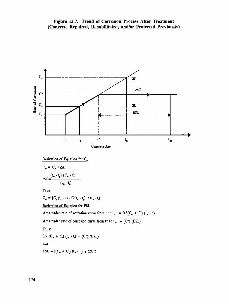
Figure 12.7. Trend of Corrosion Process After Treatment(Concrete Repaired, Rehabilitated, and/or Protected Previously)
C= _K
"_ C* ,"I , ))t=.O
©C V_ P
_' C, ESL kr
Pt_ tp t* t_ t_t
ConcreteAge
Derivationof EquationforC.
C= = Cp+AC
(t=-tp) (C=- C,)AC=
(tm-tp)
Then:
C== [Cp(t=4,)- C,(t. - tp)]/ (tp- t,)
Derivationof Equationfor ESL
Areaunderrateof corrosioncurvefromt, to t. = 0.5(Cm+ C,) (t. - t_)
Areaunderrate of corrosioncurvefromt* to t.t = (C*) (ESL)
Thus:
0.5 (C,, + C,) (t,,-t,) = (C*) (ESL)
and
ESL = [(Cm+ C,) (tin-t))] / (2C*)
174
Step 4
Use Equation 12.6 to estimate C°, the rate of corrosion corresponding to t* (age ofconcrete at time of treatment, years), milli-amperes per square foot (change t_ to t ° inEquation 12.5 to obtain Equation 12.6).
C" = [Cp (t'- t_)- C_ (t'- ta,)l / (tv - O (Equation 12.6)
Step 5
Estimate the effective service life of the newly treated concrete (ESL), years, from
Equation 12.7, assuming the rate of corrosion after the treatment will roughly remainconstant (a behavior generally expected of sealers/coatings, asphalt concrete-membranesystems, or rigid overlays. See Figure 12.7 for the derivation of Equation 12.7).
ESL = [C., + C_) (t_- t,)] / (2 C°) (Equation 12.7)
Note that if the concrete was also previously treated with sealers/coatings, asphaltconcrete-membrane systems, or rigid overlays, in the absence of background rate ofcorrosion data, it may be assumed
Cm = Cr = C"
and Equation 12.7 will give
ESL = t_ - t, (Equation 12.8)
For more accuracy, users may adjust the effective service life obtained from Equation12.8, when the new treatment is not the same as the previous treatment. The adjustmentshould be on the basis of the experience and/or the results of SHRP research by Weyerset al.4 As a default, the effective service life obtained from Equation 12.8 may beincreased 30 percent if the new treatment is a concrete overlay and the previoustreatment was a sealer/coating or asphalt concrete-membrane system. On the otherhand, the effective service life may be decreased 25 percent if the new treatment is asealer/coating or asphalt concrete-membrane system and the previous treatment was aconcrete overlay.
12.2 Case 3: Preventive Treatment
Case 3 applies to concretes which are not chloride contaminated at the bar level andwhich will receive protection against further contamination immediately. Under thiscondition, the bar-level chloride content is equal to, or less than, the corrosion threshold.Although corrosion is not present, any existing surface chlorides, can diffuse into the
175

concrete later and cause bar corrosion after the treatment. Use the following procedureto predict the effective service life of the concrete _Lfterpreventive treatment.
Step 1
Determine the set of data corresponding to the first signs of deterioration after thetreatment, as shown below.
td = age of the concrete at time to first deterioration, years (Use Equation12.9 to find ta).
td = (2.695 d1"22)/ (Zt°42P) (Equation 12.9)
See Equation 6.2 for definition of the parameters in Equation 12.9.
Sd = condition Index at time to first deterioration, 1.9
Step 2
Determine the set of data corresponding to the condition index equal to 45 after thetreatment, as shown below.
t45 = age of the concrete at condition :indexof 45, years, determined fromTable 6.1 based on the average wet resistivity of the concretesurrounding the reinforcing steel
$45 = condition index of 45
Step 3
Use the following equations to calculate Parameters A and 13in the performanceequation of the treated concrete. Alternatively, use Figures 6.3 and 6.4 to find B and A,respectively.
B = ln{[Sd(100 - $45)] / [$45(100- Sd)]} / (ta- t45) (Equation 6.6)
A = [(100 - 845) / S45] / [exp(-Bt45)] (Equation 6.7)
Step 4
Find the performance curve corresponding to Parameters A and B in Figure 7.1. Enterthe performance curve with S equal to Smand find t_, the age of the concrete at the time
176

of the maximum tolerable condition index, years. The effective service life of theconcrete after the treatment is tm- tpin which tp is the age of concrete at present, years.
177

13. Optimum Treatment and Timeof Treatment
Having determined in previous chapters (1) the concrete performance, (2) "treatmentconsideration period," (3) compatible treatment alternatives, (4) how to determine costsassociated with a treatment, and (5) the performance after the treatment, the user mustdecide what type of treatment to apply, and when to apply it within the treatmentconsideration period, for maximum cost-effectiveness. This chapter deals with thissubject through life-cycle cost analysis. Briefly, this chapter will first determine theoptimum time of treatment, for each compatible treatment; subsequently, it will comparethe corresponding life-cycle costs in order to prioritize the compatible treatments. Theseprocedures are discussed below.
For simplicity, for a compatible treatment, the user of the handbook will considertreating the concrete at only three different points in time for comparison:
1. Present time (Concrete Age = tp; Index = Sp)
2. Time corresponding to maximum tolerable condition index (Concrete Age= t_; Index = Sm)
3. Time between tv and t_ (Concrete Age = (tv + t_)/2; Index = Sp.m).
For the purpose of life-cycle cost comparison only, the user may also assume concretetreated at a point in time in the past and use the same procedure outlined in this chapterto determine the corresponding life-cycle cost.
In this handbook, the economic analysis of the three possible strategies described abovewill be done within a set time frame called the "planning horizon." The planning horizonbegins with the present time and extends for 20 years. However, if the service life of thecomponent considered for treatment is limited due to the functional features of thebridge, the planning horizon will be the remaining service life of the structure (seeChapter 3 for details).
For simplicity, this methodology assumes that after the initial treatment the concrete willonly be treated when its condition index has reached Sm(maximum tolerable). Thisassumption is justified for two reasons: (1) when costs are discounted, the timing of the
179
costs that occur far in the future do not significantly affect the life-cycle cost, and (2)when concrete is treated and protected positively, the most cost effective strategy islogically the one that gets the maximum possible use out of the treatment.
All costs associated with each strategy, including costs of repeated cycles of treatmentwithin the planning horizon (agency costs and user .costs), and salvage value of the lastcycle of treatment, are then discounted and totaled for comparison with the other'strategies. At the end of this economic analysis, the user will be able to determine theoptimum strategy, time of treatment for a compatible treatment. Also, the user will beable to prioritize the various compatible treatments, based on their life-cycle costs.Detailed procedures are described in the following sections.
13.1 Life-Cycle Cost of a Selected Treatment and Strategy
For a selected compatible treatment and a selected strategy, the life-cycle cost can beestimated by tabulating the strategy in the worksheet shown in Figure 13.1. Figures 13.2,13.3, and 13.4 are examples of tabulated strategies of "treat at tp", "treat at tm",and "treatbetween tp and tin",respectively. To estimate each strategy's life-cycle cost, use thefollowing step-by-step procedure to tabulate the three strategies for a selectedcompatible treatment in Figure 13.1.
Step 1 (Planning Horizon)
Columns 1 and 2 correspond to the 20-year planning horizon. Fill out Column 1 bystarting with the present date in the first row (1992). Fill out Column 2 by starting withYear 1 in the first row (i.e., 1).
Step 2 (Condition Index and TreatmenO
Column 3 relates to concrete condition index. Column 4 relates to the type and timingof the treatment. Follow the procedures below for the three strategies considered.
1. Treat at tp ( Example in Figure 13.2): Find the concrete condition index atpresent (Chapter 5). Fill out the first row of Column 3 with the conditionindex at present before treatment (Sp = 15), and the condition index atpresent after treatment (8.2). Fill out the first row of Column 4 with thetype of treatment considered (patch-LSDC, low-slump dense concreteoverlay).
Find the effective service life of the treated concrete (ESL, Chapter 12) (15years). Find the year to the next cycle of treatment by adding one to the
180

Figure 13.1. Worksheet for Life-Cycle Cost
Bridge Name & No.:
Year Structure Built:
Bridge Length, ft:
Two-Way ADT & Year:
Component for Treatment:
Component Area, sq ft:
Initially Built with a Protection? (What Type?)
Previously Repaired, Rehabilitated and/or Protected? (When? & What?)
W-C Ratio:
Cover Depth, Avg. & S.D., in.:
Electrical Continuity?
Year Tested:
Spalls, %:
Delams, %:
Bar-Level CL > Threshold, %:
Surface CL, Avg, & S.D., (lb/cy):
181
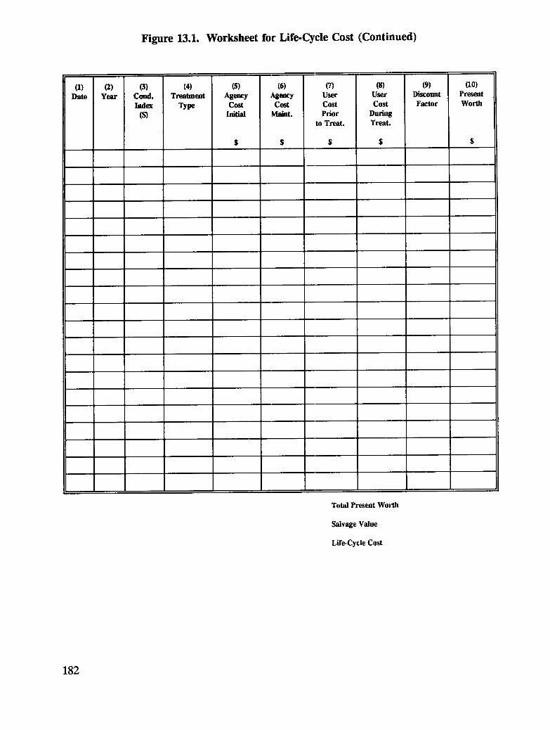
Figure 13.1. Worksheet for Life-Cycle Cost (Continued)
(1) (2) (3) (4) (s) (6) (_3 (s) (9) (10)Date Year Cmul. Treatment Agmcy Agency User User Discount Present
Index Type Cost Cost Cost Cost Factor Worth(S) Initial Mahtt. Prior During
to Treat. Treat.
$ $ $ $ $
Total Present Worth
Salvage Value
Life-CydeCost
182

Figure 13.2. Example of Tabulated Treatment Strategy (Treat at tp)
(1) (2) (3) (4) (_ (6) 03 (8) (9) (10)Date Year Cond. Treatment Ageacy Agency User User Discount Present
Index Type Cost Cost Cost Cost Factor Worth(S) Initial Maint. Prior During
to Treat. Treat.$ $ $ $ $
1992 1 15 Patch- 101,955 26,666 1 128,6218.2 LSDC
1993 2 10.0 0.961
1994 3 11.8 0.925
1995 4 13.6 0.888
1996 5 15.4 0.854
1997 6 17.2 0.821
1998 7 19.0 0.790
1999 8 20.8 1,274 0.759 966
2000 9 22.6 1,775 0.730 1,295
2001 10 24.4 2,413 0.702 1,693
2002 11 26.2 3,207 0.675 2,164
2003 12 28.0 4,184 0.649 2,715
2004 13 29.8 5,368 0.624 3,349
2005 14 31.6 6,788 0.600 4,072
2006 15 33.4 8,472 0.577 4,888
2007 16 35 Patch- 214,033 46,666 0.555 144,68711.8 LSDC
2008 17 13.3 0.534
2009 18 14.8 0.513
2010 19 16.3 0.493
2011 20 17.8 0.474
Total Present Worth 294,450
Salvage Value 82,380
Life-Cycle Cost 212,070
183

Figure 13.3. Example of Tabulated Treatment Strategy (Treat at tin)
(1) (2) O) (4) (5) (6) (7) (8) (9) (I0)Date Year Cond. Treatment Agency Agency User User Discount Present
Index Type Cost Cost Cost Cost Factor Worth(S) Initial Mnint. Prior During
to Treat. Treat.$ $ $ $ $
1992 1 15 1
1993 2 18 0.961
1994 3 21 1,324 0.925 1,224
1995 4 24 2,259 0.888 2,005
1996 5 27 3,619 0.854 3,090
1997 6 30 5,516 0.821 4,528
1998 7 33 8,076 0.790 6,380
1999 8 35 Patch- 214,033 46,666 0.759 197,87011.8 LSDC
2000 9 14.1 0.730
2001 10 16.4 0.702
2002 U 18.7 0.675
2003 12 21.0 1,323 0.649 858
2004 13 23.3 2,006 0.624 1,251
2005 14 25.6 2,923 0.600 1,753
2006 15 27.9 4,125 0.577 2,380
2007 16 30.2 5,662 0.555 3,142
2008 17 32.5 7,595 0.534 4,055
2009 18 35 Patch- 214,033 46,666 0.513 133,73811.8 LSDC
2010 19 14.1 0.493
2011 20 16.4 0.474
Total Present Worth 362,274
Salvage Value 86,499
Life-Cycle Cost 275,774
184

Figure 13.4 Example of Tabulated Treatment Strategy (Treat between tp and tm)
(1) (2) O) (4) (5) (6) (7) (8) (9) (10)Date Year Cond. Trenimmt Agency Agency User User Discount Present
Index Type Cost Cost Cost Cost Factor Worth(S) Initial Maint. Prior During
to Treat. Treat.S S S $ S
1992 1 15 1
1993 2 18 0.961
1994 3 21 1,324 0.925 1,218
1995 4 24 Patch- 139,230 33,333 0.888 153,25311.8 LSDC
1996 5 13.7 0.854
1997 6 15.6 0.821
1998 7 17.5 0.790
1999 8 19.4 0.759
2000 9 21.3 1,401 0.730 1,022
2001 10 23.2 1,972 0.702 1,384
2002 11 25.1 2,702 0.675 1,823
2003 12 27.0 3,617 0.649 2,347
2004 13 28.9 4,748 0.625 2,967
2005 14 30.8 6,126 0.600 3,675
2006 15 32.7 7,783 0.577 4,490
2007 16 35 Patch- 214,033 46,666 0.555 144,68711.8 LSDC
2008 17 13.7 0.534
2009 18 15.6 0.513
2010 19 17.5 0.493
2011 20 19.4 0.474
Total Present Worth 316,866
Salvage Value 72,083
Life-Cycle Cost 244,782
185

effective service life of the treated concrete (1 + 15 .'=Year 16). Fill out thoseboxes in Columns 3 and 4 which correspond to the year of next cycle of treatment(Year 16) with the maximum tolerable condition inde.x (S= = 35), the conditionindex after treatment (11.8; use Chapter 11 1Lodecompose S,, and Chapter 5 todetermine the index just after treatment), and the type of treatment in the nextcycle of treatment (patch LSDC).
Find the approximate concrete condition index for each consecutive yearafter the treatment from Equation 13.1. Fill out the appropriate boxes ofColumn 3 with the approximate condition indices determined (10.0 through33.4).
SA_rr_.,_.t = [(Sin- Index just after Treatment) x (No. of Years afterTreatment) / (Effective Service Life after Treatment)] +[Index just after Treatment] (Equation 13.1)
[Equation 13.1 assumes a linear relation between condition index and time.This approximation is justified, since usually after the treatment the slopeof the "S" curve applies. However, if the exact value of condition index isrequired, Equations 6.1, 6.3, and 6.4 may be used.]
Do not repeat treating the concrete, if the effective service life of thetreated concrete (in this example 15 years) is more than the remainingyears in the consideration period (in this example 5 years).
2. Treat at t m (Example in Figure 13.3): Find concrete condition index foreach consecutive year starting with the present year, l:p,and ending with tm(Chapter 6). Fill out the appropriate boxes of Colurrm 3 with the conditionindices determined (Sp = 15 through Sm= 35). Also, fill out the box for Smwith the index just after the treatment (11.8; use Chapter 11 to decomposeSmand Chapter 5 to determine the index just after treatment). Fill out thebox in Column 4 that corresponds to Smwith the type: of treatment (patch-LSDC).
Find the effective service life of the treated concrete (ESL, Chapter 12) (10years). Find the year to the next cycle of treatment by adding the effectiveservice life of the treated concrete to the year of treatment (10 + 8 = Year18). Fill out those boxes in Columns 3 and 4 which correspond to the year ofnext cycle of treatment (Year 18) with the maximum tolerable condition index(S= = 35), the condition index after treatment (11.8), and the type oftreatment in the next cycle (patch-LSDC).
Find the approximate concrete condition index for each consecutive yearafter the treatment from Equation 13.1. Fill out the appropriate boxes ofColumn 3 with the approximate condition indices determined (14.1 through32.5).
186

S^_r r_,_,,_t = [(Sin- Index just after Treatment) x (No. of Years afterTreatment) / (Effective Service Life after Treatment)] +[Index just after Treatment] (Equation 13.1)
Do not repeat treating the concrete if the effective service life of thetreated concrete (in this example 10 years) is more than the remainingyears in the consideration period (in this example 3 years).
3. Treat between tp and t m (Example in Figure 13.4): Find the concretecondition index for each consecutive year starting with the present year, tp,and ending with (tp + tm)/ 2 (Chapter 6). Fill out the appropriate boxesof Column 3 with the condition indices determined (Sp = 15 through Sp_m=24). Also, fill out the box for Sp_mwith the index just after the treatment(11.8; use Chapter 11 to decompose Sp-mand Chapter 5 to determine theindex just after treatment). Fill out the box in Column 4 that correspondsto Sp_mwith the type of treatment (patch-LSDC).
Find the effective service life of the treated concrete (12 years; useChapter 12 to determine the ESL). Find the year to the next cycle oftreatment by adding the effective service life of the treated concrete to theyear of treatment (12 + 4 = Year 16). Fill out those boxes in Columns 3and 4 which correspond to the year of next cycle of treatment (Year 16)with the maximum tolerable condition index (Sin= 35), the condition indexafter treatment (11.8), and the type of treatment in the next cycle (e.g.,patch-LSDC).
Find the approximate concrete condition index for each consecutive yearafter the treatment from Equation 13.1. Fill out the appropriate boxes ofColumn 3 with the approximate condition indices determined (13.7 through32.7).
SAlter Treatm_at = [(Sm- Index just after Treatment) x (No. of Years afterTreatment) / (Effective Service Life after Treatment)] +[Index just after Treatment] (Equation 13.1)
Do not repeat treating the concrete if the effective service life of thetreated concrete (in this example, 12 years) is more than the remainingyears in the consideration period (in this example, 5 years)
Step 3 (Agency Costs)
Columns 5 and 6 relate to agency costs. Fill out the appropriate boxes of Column 5 withthe cost associated with the application of the treatment (Chapter 9).
187

Fill out the appropriate boxes of Column 6 with the annual cost ofmonitoring/maintaining the treatment (Chapter 9). For example, in Figures 13.2, 13.3and 13.4 there were no agency maintenance costs.
Step 4 (User Costs Prior to TrearmenO
Column 7 is for user costs prior to the treatment. Using the condition index given inColumn 3, estimate the user costs prior to the treatment for each consecutive year in theplanning horizon (Chapter 10).
Step 5 (User Costs During Treatment)
Column 8 is for user costs during the treatment (Chapter 10).
Step 6 (Discount Factor)
Column 9 is for the discount factor. Using the equation given below, find the discountfactor for each consecutive year in the planning horizon; alternatively, use Figure 13.5.
DF = 1 / (1 + EI) *-1 (Equation 13.2)
where
DF = discount factor
EI = effective interest rate = interest rate minus inflation rate
n = number of each consecutive year in the planning horizon
Fill out the boxes of Column 9 with the discount factors.
Step 7 (Present Worth)
Column 10 gives the sum of the costs in each consecutive year in "current dollars"(present worth). Multiply the sum of all costs in each consecutive year by thecorresponding discount factor, and fill out the boxes of Column 10 with the products.
188

Figure 13.5. Discount Factors
Consecutive years El I -- 1% El = 2% E1 = 3% E1 = 4% E1 = 5%
1 1.000 1.000 1.000 1.000 1.000
2 0.990 0.980 0.971 0.962 0.952
3 0.980 0.961 0.943 0.925 0.907
4 0.971 0.942 0.915 0.889 0.864
5 0.961 0.924 0.888 0.855 0.823
6 0.951 0.906 0.863 0.822 0.784
7 0.942 0.888 0.837 0.790 0.746
8 0.933 0.871 0.813 0.760 0.711
9 0.923 0.853 0.789 0.731 0.677
10 0.914 0.837 0.766 0.703 0.645
11 0.905 0.820 0.744 0.676 0.614
12 0.896 0.804 0.722 0.650 0585
13 0.887 0.788 0.701 0.625 0557
14 0.879 0.773 0.681 0.601 0.530
15 0.870 0.758 0.661 0577 0.505
16 0.861 0.743 0.642 0555 0.481
17 0.853 0.728 0.623 0-534 0.458
18 0.844 0.714 0.605 0513 0.436
19 0.836 0.700 0587 0.494 0.416
20 0.828 0.686 0570 0.475 0.396
E1 = Effective Interest Rate = Interest rate - Inflation rate
189
Step 8 (Total Present Worth)
Add up all costs in Column 10. This is the total present worth, as shown in the bottomof Figure 13.1.
Step 9 (Salvage Value)
Use the procedure described below to determine the discounted salvage value of the lasttreatment in the last year of the plamaing horizon (i.e., the 20th year), as shown in thebottom of Figure 13.1. Salvage value applies to the remaining useful life of the treatmentbeyond the planning horizon, and is determined from the following equation.
SLVG = (COST) (RS/ESL) (DF20) (Equation 13.3)
where
SLVG = salvage value, present worth, dollars
COST = cost of last treatment (sum of all costs in the year of last treatmentbefore discounting), dollars
RS = remaining effective service life of the concrete component aftertreatment (last treatment'.) beyond the planning horizon, years
ESL = estimated effective service life of treated concrete, years
DF20 = discount factor corresponding to the last year in the planning horizon(i.e., 20th year)
Step 10 (Life-Cycle Cost)
Subtract the discounted salvage value (Step 9) from the total present worth (Step 8) tofind the life-cycle cost for the strategy considered. Fill out the "Life-Cycle Cost" box inthe bottom of Figure 13.1.
Step 11 (Life-Cycle Cost Comparison)
Compare the life-cycle costs of the three strategies (i.e., treat at tp, treat at tin,and treatbetween ta,and t_), and select the strategy with the minimum life-cycle cost.
190

14. Worked Example
The example in this chapter illustrates how the methodology introduced in this handbookis applied to make a decision to treat a concrete bridge component.
[To convert to metric units in this example: one square foot is 0.929 square meters; oneinch is 2.54 centimeters; one pound per cubic yard is 0.59 kilograms per cubic meter; onedollar per square foot is 10.76 dollars per square meter; and one foot is 0.3 meters.]
14.1 General Description of the Example
The concrete bridge component to be examined is a bridge deck with an area of 10,000square feet. The concrete bridge deck was placed in 1978, and it contains "black"reinforcing steel. The concrete is a conventional concrete with a specified water-cementratio of 0.45 (assume actual water-cement ratio = 0.45 + 0.03 = 0.48, unless fieldinformation exists) and a specified bar cover depth of 1.5 inches. The concrete has notreceived any treatment since 1978.
The average two-way daily traffic volume across the bridge is 15,000 vehicles. Theconcrete deck has been exposed to de-icing salt during its service, but backgroundchlorides do not exist in the concrete. Reinforcing steel corrosion-induced deteriorationhas been present and is a concern. The expected remaining service life of the structuredue to bridge functional features is 50 years (i.e., unlimited remaining service life, seeChapter 3).
The highway agency that owns the bridge would like to determine when the bridgeshould be treated against chloride-induced corrosion and what type of treatment shouldbe applied.
191

14.2 Systematic Procedure to Determine Type and Timing of Treatment
A: Test Concrete (Chapter 4)
The concrete deck was tested in 1992 (present year) and the following results wereobtained.
Visual Inspection:
• Spalls (1 percent of deck area)• Patches (none)• Scaling (none)• Pop-outs (none)• Cracks (minor, no active cracks)• Wheeltrack wear (not significant)
Delamination Survey
• Delamination (5 percent of the deck area)
Cover Depth
• Average bar cover depth (1.40 inches)• Standard deviation (0.50 inches)
Reinforcing Steel Electrical Continuity
• O.K.
Chloride Profiles
• Average chlorides at top bars (0.0875 percent of concrete weight, or 3.5 pounds percubic yard)
• Percent of concrete samples at top bars with chlorides higher than the threshold of0.035 percent of concrete weight, or 1.4 pounds per cubic yard (40 percent)
• average surface chlorides (0.250 percent of concrete weight, or 10 pounds per cubicyard)
standard deviation (0.05 percent of concrete weight, or 2 pounds per cubic yard)
192
Corrosion Potential Survey
• Not conducted
Rate of Corrosion Measurements
• Not conducted
Permeability/Resistivity Test
• Not conducted
Overall Evaluation: Non-corrosion related deterioration is not significant. Thus,continue using this manual.
B: Condition Determination (Chapter 5)
Use Equation 5.2, or Figure 5.1, to determine the concrete condition index.
S = [ CL + 2.5(DELAM) + 7.5(SPALL)] / 8.5
S = [40 + 2.5(5) + 7.5(1)] / 8.5
S = 7.1
C: Prediction of Performance (Chapter 6)
Use Section 6.2, "Concrete not Repaired, Rehabilitated and/or Protected Previously andwithout a Special Protection."
Step 1
tv = 1992-1978 = 14 years
Sp = 7.1
Since Spmore than 1.9, use Steps 2 and 3 in Section 6.2.
193

Step 2
Use Equation 6.2, or Figure 6.1, to f:ind t i (concrete age at first sign of deterioration).
h = [(2.695 d''22t°'2') / (Zt°42p)]O.:_265
td = {[2.695 (1.4 - 1.282 X0.50)122X 14TM] / [(0.250 + 1.282 x 0.05)o.42x 0.48} 0.8265
h = 7.5 years, and
Sd = 1.9
Step 3
Use Equations 6.4 and 6.5 to find Parameters B and A. Alternatively, use Figures 6.3and 6.4.
B = ln{[Sd(100 - Sp)] / [Sp(100- Sa)]} / (h- tp)
B = ln{[1.9(100- 7.1)] / [7.1(100- 1.9)]} / (7_';- 14)
B = 0.21
A = [(100-Sp) / (Sp]/[exp(-Btp)]
A = [(100 - 7.1) / 7.1] / [exp(-0.21 x 14)]
A = 245.3
Thus, the concrete performance equation is:
St = 100 / [ 1 + 245.3 exp(-0.21 t)]
D: Evaluation of Performance (Chapter 7)
Treatment Consideration Period = t_ - tp
Find tmfrom Equation 7.2, or Figure 7.1, assuming Sm= 35.
tm= -{In[(100 - Sm)/ (A S,,)]} / B
tm = -{In[(100 - 35) / (245.3 x 35)]} / 0.21
194

t_ = 23.3 years, and
= 14 years
Treatment Consideration Period = 23.3 - 14 = 9.3 years (i.e., 1992 to 2001)
Use the rest of the handbook to determine the timing of the treatment within thetreatment consideration period, for a compatible treatment.
E: Compatible Treatment Alternatives (Chapter 8)
Use Table 8.1 to screen out the incompatible treatment alternatives. The rest of thisexample will only consider one alternative (patching and low-slump dense concreteoverlay) in order to determine its optimum timing for maximum cost-effectiveness. Thesame procedure can be used to determine the timing and life-cycle costs of eachcompatible alternative for comparison.
F: Cost Items Associated with Treatment, Agency Costs (Chapter 9)
• Removing/patching deteriorated concrete ($35 per square foot of deterioratedconcrete)
• Scarifying deck ($0.75 per square foot of deck)• Placing and curing 1.5 in. LSDC overlay ($2.85 per square foot of deck)• Traffic control ($2.00 per square foot of deck area)
G: Cost Items Associated with Treatment, User Costs (Chapter 10)
Prior-to-Treatment Costs
Use Equation 10.2, or Figure 10.3.
U2 = K2 [S / Sm]4 [365 qo]
where
U2 = user costs, dollars per yearS. = 35qo = 15,000 vehicles per dayK2 = a t_K,
Assume
tf = 0.06 minutes (free flow travel time across 300 ft bridge),
195

KI = $0.1666 per minute per vehicle, anda = 50% (50 percent reduction in travel time).
This will give
K2 = 0.50 x 0.06 x 0.1666 = $0.005 per vehicle.
then
Us = (0.005) [S/35]4 [365 x 15,000]U2 = 27,375 [S/35]'
Use the relation above, or Figure 10.3, to find Us for a giwm S when tabulating astrategy in I, below.
During-Treatment Costs
Use Equation 10.2, or Figure 10.1.
UI = Klt_toqo
where
U_ = user costs, dollarsK1 = $0.1666 per minute per vehicletc = duration of repair, daysqo = 15,000 vehicles per daytt = 2 minutes (assume detour around the bridge)
then
U_ = (0.1666)(2)(to)(15,000)UI = 4999.5 tc
Use the relation above, or Figure 10.1, to find UI for a given tcwhen tabulating astrategy in Part I, below.
H: Prediction of Performance, Treated Concrete (Chapter 12)
Use Case 1, "Concrete not Repaired, Rehabilitated and/or Protected Previously."Condition 4, in which the rate of corrosion decreases gradually after the treatment,applies to this example. Use Equation 12.4, or Figure 12.6, to predict the effectiveservice life (ESL) after the treatment (i.e., years to condition index of Sm= 35 after thetreatment).
196
ESL = {[(t" - to)2 + K(t_-to)2]°' - (t° - to) } / K
Assume K = -1/5 (ratio of slope of rate of corrosion line after treatment to slope of rateof corrosion line before treatment). Since td = 7.5 years (Part C), to = 5 years (Figure12.3), and t_ = 23.3 years (Part D), then:
ESL = {[(t"- 5)2 + (-1/5)(23.3-5)2] °'- (t'-5) } / (-1/5)ESL = 5 {(t'- 5)-[(t'- 5)2- 70]0.5}
Use the relation above to find ESL for a given t* when tabulating a strategy in I, below.
I: Optimum Treatment and Time of Treatment (Chapter 13)
Consider treating the deck with patch-LSDC (patching and low-slump dense concreteoverlay; contaminated concrete left in place) at three different points in time (threestrategies) as shown below.
• Concrete age = tp (age 14 years, year 1992)• Concrete age = t_ (age 23.3 years, year 2001)• Concrete age = (tp + t_)/2 (age 18.65 years, year 1997)
Use Section 13.1 and the worksheet in Figure 13.1, to estimate the life-cycle cost of eachstrategy. (Results are shown in Figures 14.1, 14.2, and 14.3 at the end of this chapter.)
Step 1, Planning Horizon (All Strategies)
From Chapter 3, since the remaining service life of the bridge is 50 years (higher than 30years), the planning horizon is 20 years. Fill out Column 1 in Figure 13.1 by startingwith the year 1992 and ending with the year 2011. Fill out Column 2 by starting withYear 1 and ending with Year 20.
Step 2, Condition Index and Treatment
Strategy, Treat at tp
Fill out the first row of Column 3 with the condition index at present before treatment(S = 7.1) and after treatment (S = 4.7). Fill out the first row of Column 4 with the typeof treatment considered (patch-LSDC).
197

From Part H, the effective service life of concrete after treatment, ESL, is
ESL = 5 {(t'- 5)-[(t" - 5) 2- 70] °5}
where t" = tp = 14 years
ESL = 5 {(14- 5)-[(14 - 5)2- 70] °s}ESL = 28 years
Find the year to the next cycle of treatment by adding one to the effective service life ofthe concrete after treatment (1 + 28 = Year 29). Therefi)re, no further treatment isrequired during the planning horizon.
Find the approximate concrete condition index for each co:asecutive year after thetreatment from Equation 13.1.
S^f_rrt_,-_t = [(Sin - Index just after Treatment) x (No. of Years after Treatment)/(Effective Service Life after Treatment)] + [Index just aftertreatment]
SAe_rr_t_ = [(35 - 4.7) X (NO. of Years after Treatment) / (28)] + [4.7]
S^f_ r,.,_,_, = (1.08) x (No. of Years after Treatment) + 4.7
No. of Years After S After Treatment Year in Planning HorizonTreatment
1 5.8 22 6.9 33 7.9 44 9.0 55 10.1 66 11.2 77 12.3 88 13.3 99 14.4 1010 15.5 1111 16.6 1212 17.7 1313 18.7 1414 19.8 1515 20.9 1616 22.0 1717 23.1 1818 24.1 1919 25.2 20
198
Strategy, Treat at t m
Use Equation 6.1, or Figure 7.1, to predict the concrete condition index prior totreatment.
St = 100 / [1 + A exp(-Bt)]
Concrete Age, t S Before Treatment Year in Planning Horizon
14 7.1 115 8.6 216 10.4 317 12.6 418 15.0 519 17.9 620 21.2 721 24.9 822 29.0 923 33.5 1024 38.3 > Sm= 35 11
Fill out the appropriate boxes of Column 3 with the condition indices of S = 7.1 throughS = 33.5. Also, fill out the box for S = 33.5 with the index just after treatment (i.e.,11.8). Fill out the box in Column 4 that corresponds to S = 33.5 with the type oftreatment, patch-LSDC.
From Part H, the effective service life of concrete after treatment, ESL, is:
ESL = 5 {(t*- 5)-[(t" - 5)2- 70]°5}
where t* = tm = 23.3 years
ESL = 5 {(23.3- 5) -[(23.3- 5)2- 70]°5}
ESL = 10 years
The year to the next cycle of treatment is 10 + 10 = Year 20. Fill out those boxes inColumns 3 and 4, which correspond to Year 20 with Sm= 35 and the type of treatment(patch-LSDC), respectively.
Find the approximate concrete condition index for each consecutive year after thetreatment using Equation 13.1.
SAferr_,=t = [(Sm- Index just after Treatment) x (No. of Years afterTreatment)/(Effective Service Life after Treatment)] + [IndexJust after Treatment]
199

S^_,rr_.,t_t = [(35 - 11.8) x (No. of Years after Treatment) / (10)] + [11.8]
SA_rr_.,t_ t = (2.32) X (No. Of Years after Treatment) + 11.8
No. of Years After S After Treatment Year in Planning HorizonTreatment
1 14.1 112 16.4 123 18.7 134 21.0 145 23.3 156 25.6 167 27.9 178 30.2 189 32.5 19
10 35 20
Strategy, Treat between tp and t_
Use Equation 6.1, or Figure 7.1, to predict the concrete condition index prior totreatment.
St = 100/[1 + A exp(-Bt)]
Concrete Age, t S Before Treatment Year in Planning Horizon
14 7.1 115 8.6 216 10.4 317 12.6 418 15.0 519 17.9 6
Fill out the appropriate boxes of Column 3 with the condition indices of S = 7.1 throughS = 17.9. Also, fill out the box for S = 17.9 with the index just after treatment (i.e.,10.3). Fill out the box in Column 4 that corresponds to S = 17.9 with the type oftreatment, patch-LSDC.
From Part H, the effective service life of concrete after treatment, ESL, is
ESL = 5 {(t °- 5)-[(t °- 5)2- 70] °5)
200
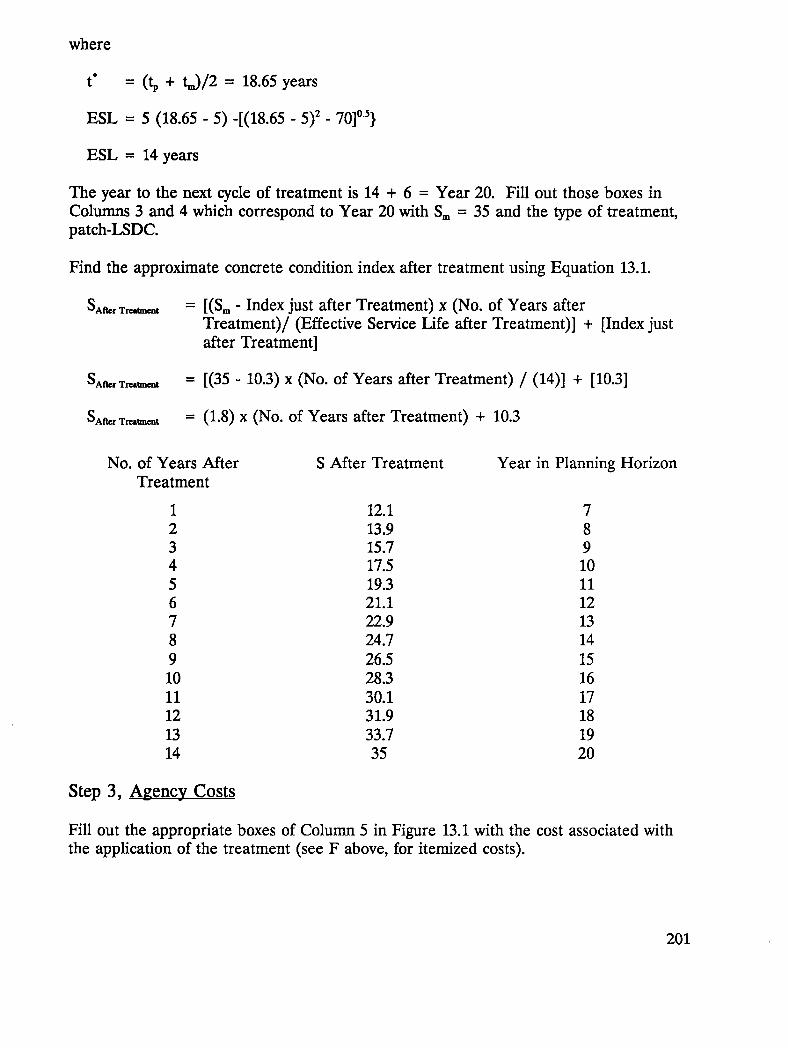
where
t* = (tp + t_)/2 = 18.65 years
ESL = 5 (18.65- 5)-[(18.65- 5)2- 70]°'}
ESL = 14 years
The year to the next cycle of treatment is 14 + 6 = Year 20. Fill out those boxes inColumns 3 and 4 which correspond to Year 20 with S,, = 35 and the type of treatment,patch-LSDC.
Find the approximate concrete condition index after treatment using Equation 13.1.
SA_rx_,_t = [(S,, - Index just after Treatment) x (No. of Years afterTreatment)/(Effective Service Life after Treatment)] + [Index justafter Treatment]
SA_rT,_,t = [(35 - 10.3) X(No. of Years after Treatment) / (14)] + [10.3]
SA_rx_,_-c,t = (1.8) x (No. of Years after Treatment) + 10.3
No. of Years After S After Treatment Year in Planning HorizonTreatment
1 12.1 72 13.9 83 15.7 94 17.5 105 19.3 116 21.1 127 22.9 138 24.7 149 26.5 1510 28.3 1611 30.1 1712 31.9 1813 33.7 1914 35 20
Step 3, Agency Costs
Fill out the appropriate boxes of Column 5 in Figure 13.1 with the cost associated withthe application of the treatment (see F above, for itemized costs).
201

Strategy, Treat at tp
DELAM = 5%
SPALL = 1%
Total Area Deteriorated = 5 + 1 = 6%
1. Removing and patching concrete: (6 percent of 10,000 square feet at $35 persquare foot) = $21,000
2. Concrete overlay (10,000 square feet at $5.60 per square foot, the total costs forscarifying the deck, placing and curing the overlay, and providing traffic control) =$56,000
Total Agency Cost = 21,000 + 56,000 = $77,00,0
Strategy, Treat at t m
Use Equations 11.1 through 11.3 to decompose the condition index of S = 33.5.
CL = 5S
CL = 5 (33.5) = 167.5 > 100, then, CL = 100%
DELAM= (8.5S-CL) / (2.5+ 7.5/N)DELAM = (8.5 x 33.5- 100) / (2.5 + 7.5/4) = 42.2%
SPALL -- DELAM / NSPALL = 42.2 / 4 = 10.5%
Total Area Deteriorated = 42.5 + 10..5= 53%
1. Removing and patching concrete (53 percent of 10,000 square foot at $35 persquare foot) = $185,500
2. Concrete overlay (10,000 square feet at $5.60 per square foot) = $56,000
Total Agency Cost = 185,500 + 56,000 = $241,500
Use the same agency cost when treatment is repeated at Sin,with sufficient accuracy.
Strategy, Treat between tp and t_
Use Equations 11.1 through 11.3 to decompose the condition index of S = 17.9.
CL= 5S
CL = 5 (17.9) = 89.5%
DELAM = (8.5 S- CL) / (2.5 + 7.5/N)
202
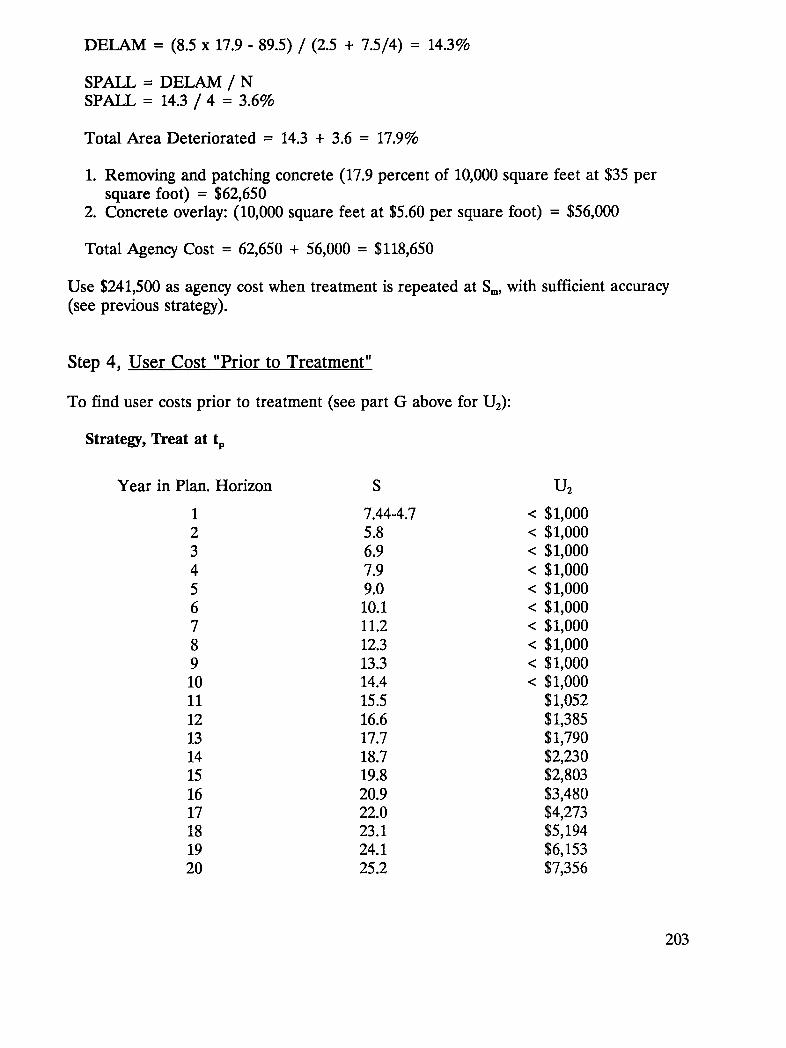
(8.5 x 17.9 - 89.5) / (2.5 + 7.5/4) = 14.3%
DELAM / N14.3 / 4 = 3.6%
Deteriorated = 14.3 + 3.6 = 17.9%
and patching concrete (17.9 percent of 10,000 square feet at $35 perfoot) = $62,650
overlay: (10,000 square feet at $5.60 per square foot) = $56,000
Cost = 62,650 + 56,000 = $118,650
agency cost when treatment is repeated at Sin,with sufficient accuracystrategy).
Cost "Prior to Treatment"
costs prior to treatment (see part G above for U2):
Treat at tp
Plan. Horizon S U2
1 7.44-4.7 < $1,0002 5.8 < $1,0003 6.9 < $1,0004 7.9 < $1,0005 9.0 < $1,0006 10.1 < $1,0007 11.2 < $1,0008 12.3 < $1,0009 13.3 < $1,00010 14.4 < $1,00011 15.5 $1,05212 16.6 $1,38513 17.7 $1,79014 18.7 $2,23015 19.8 $2,80316 20.9 $3,48017 22.0 $4,27318 23.1 $5,19419 24.1 $6,15320 25.2 $7,356
203

Fill out the boxes of Column 7 with the user costs.
Strategy, Treat at tm
Year in Plan. Horizon S U2
1 7.1 < $1,0002 8.6 < $1,0003 10.4 < $1,0004 12.6 < $1,0005 15.0 < $1,0006 17.9 $1,8727 21.2 $3,6848 24.9 $7,0129 29.0 $12,90210 33.5-11.8 < $1,00011 14.1 < $1,00012 16.4 $1,31913 18.7 $2,23014 21.0 $3,54715 23.3 $5,37616 25.6 $7,83517 27.9 $11,05318 30.2 $15,17419 32.5 $20,35220 35.0-11.8 < $1,000
Fill out the boxes of Column 7 with the user costs.
Strategy, Treat between tp and t,
Year in Plan. Horizon S U2
1 7.1 <$1,0002 8.6 < $1,0003 10.4 < $1,0004 12.6 < $1,0005 15.0 < $1,0006 17.9-10.3 <$1,0007 12.1 < $1,0008 13.9 < $1,0009 15.7 $1,108
204

Year in Plan. Horizon S U2
10 17.5 $1,71011 19.3 $2,53112 21.1 $3,61513 22.9 $5,01614 24.7 $6,78915 26.5 $8,99616 28.3 $11,70117 30.1 $14,97418 31.9 $18,89019 33.7 $23,52820 35.0-11.8 <$1,000
Fill out the boxes of Column 7 with the user costs.
Step 5, User Cost "During Treatment"
Fill out the appropriate boxes of Column 8 with the user costs during the treatment (SeeG above for U_).
Strategy, Treat at tp
To find user costs during the treatment
Concrete Removal/Patching at 200 square feet per day = 3 daysOverlay Placing/Curing at 2,000 square feet per day = 5 days
Total time (to) = 8 days
U1 = $40,000
Strategy, Treat at t.
To find user costs during the treatment
Concrete Removal/Patching at 200 square feet per day = 27 daysOverlay Placing/Curing at 2,000 square feet per day = 5 days
Total time (to) = 32 days
U1 = $160,000
Use the same user cost when treatment is repeated at Sin.
205

Strategy, Treat between tp and tm
To find user costs during the treatment
Concrete Removal/Patching at 200 square feet per day = 9 daysOverlay Placing/Curing at 2,000 square feet peg day = 5 days
Total time (to) = 14 days
U1 = $70,000
Use $160,000 as user cost during treatmeat when _Lreatmenl:is repeated at Sin.
Step 6, Discount Factor (All Strategies)
Find the discount factor for each consecutive year in the consideration period, assumingan interest rate of 7 percent and an inflation rate of 3 percent, or an effective interestrate of 7 - 3 = 4 percent (Equation 13.2, or Figure 13.5). Fill out the boxes in Column 9with the discount factors.
Step 7, Present Worth (All Strategies)
Multiply the sum of all costs in each consecutive 3'ear by the corresponding discountfactor, and fill out the boxes of Column 10 with the products.
Step 8, Total Present Worth (All Strategies)
Add up all the costs in Column 10 to find the total present worth of eachstrategy.
Step 9, Salvage Value
Find discounted salvage value of the last treatment and fill out the corresponding box inthe bottom of Figure 13.1 (Equation 13.3).
Strategy, Treat at tp
SLVG = (COST) (RS/ESL) (DV2o)
SLVG = ($77,000 + $40,000) [(28- 20)/28] (0.474)SLVG = $15,845
206

Strategy, Treat at t m
SLVG = ($241,500 + $160,000) [(10- 1)/10] (0.474)SLVG = $171,059
Strategy, Treat between tpand t m
SLVG = ($241,500 + $160,000)[(14- 1)/14] (0.474)SLVG = $176,716
Step 10, Life-Cycle Cost
Subtract the discounted salvage value (Step 9) from the total present worth (Step 8) tofind the life-cycle cost for each strategy. Fill out the "Life-Cycle Cost" box in the bottomof Figure 13.1.
Strategy, Treat at tp
Life-Cycle Cost = $136,074- $15,845 = $120,229
Strategy, Treat at t.,
Life-Cycle Cost = $526,961 - $171,066 = $355,895
Strategy, Treat between tp and t m
Life-Cycle Cost = $399,431 - $176,716 = $222,715
Step 11, Life-Cycle Cost Comparison
If the deck is treated at the present (year 1992), the life-cycle cost will be 54 percent ofthe life-cycle cost if it were treated in 1997, and it will be 34 percent of the life-cycle costif it were treated in 2001.
Treatment Time Life Cost, dollars
1992 120,2291997 222,7152001 355,895
207
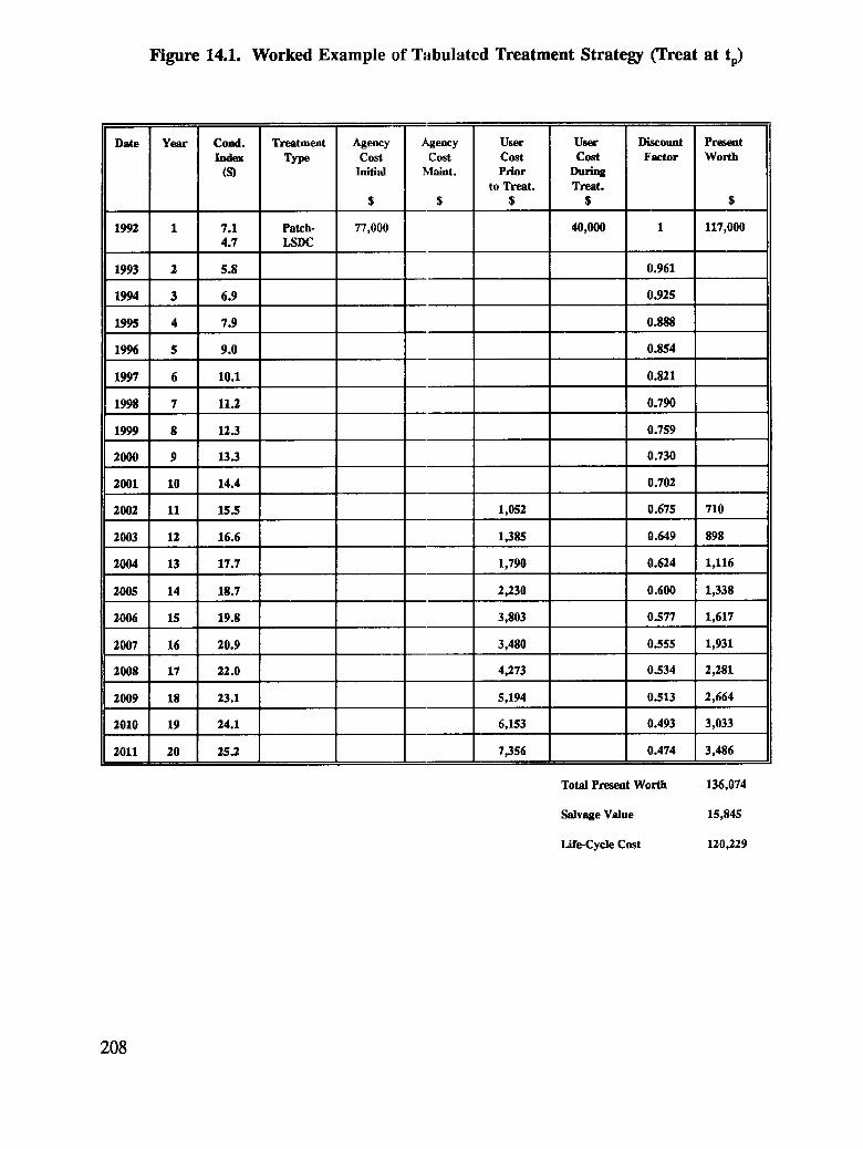
Figure 14.1. Worked Example of Tabulated Treatment Strategy (Treat at tp)
Date Year Cond. Treatment Agency Agency User User Discount PresentIndex Type Cost Cost Cost Cost Factor Worth
(S) Initial Maint. Prior Duringto Treat. Treat.
$ $ $ $ $
1992 1 7.1 Patch- 77,000 40,000 1 117,0004.7 LSDC
1993 2 5.8 0.961
1994 3 6.9 0.925
1995 4 7.9 0.888
1996 5 9.0 0.854
1997 6 10.1 0.82I
1998 7 11.2 0.790
1999 8 I2.3 0.759
2000 9 13.3 0.730
2001 IO 14.4 0.702
2002 11 15.5 1,052 0.675 710
2003 12 16.6 1,385 0.649 898
2004 13 17.7 1,790 0.624 I,lI6
2005 14 18.7 2,230 0.600 1,338
2006 15 19.8 3,803 0.577 1,617
2007 16 20.9 3,480 0.555 1,93I
2008 17 22.0 4,273 0.534 2,281
2009 18 23.1 5,194 0.513 2,664
2010 19 24.1 6,153 0.493 3,033
2011 20 25.2 7,356 0.474 3,486
Total Present Worth 136,074
Salvage Value 15,845
IMe-Cycle Cost 120,229
208

Figure 14.2. Worked Example of Tabulated Treatment Strategy (Treat at tm)
Date Year Cund. Treatment Agency Agency User User Discount PresentIndex Type Cost Cost Cost Cost Factor Worth
(S) Initial Maint. Prior Duringto Treat. Treat.
$ $ $ $ $
1992 1 7.1 1
1993 2 8.6 0.961
1994 3 10.4 0.925
1995 4 12.6 0.888
1996 5 15.0 0.854
1997 6 17.9 1,872 0.821 1,536
1998 7 212 3,684 0.790 2,910
1999 8 24.9 7,012 0.759 5,332
2000 9 29.0 12,982 0.730 9,476
2001 10 33.5 Patch- 241,500 160,000 0.702 281,85311.8 LSDC
2002 11 14.1 0.675
2003 12 16.4 1,319 0.649 856
2004 13 18.7 2,230 0.624 1,391
2005 14 21.0 3,547 0.600 2,128
2006 15 23.3 5,376 0.577 3,101
2007 16 25.6 7,835 0.555 4,348
2008 17 27.9 I1,053 0.534 5,902
2009 18 30.2 15,174 0.513 7,784
2010 19 32.5 20,352 0.493 10,033
2011 20 35 Patch- 241,500 160,000 0.474 190,31111.8 LSDC
Total Present Worth 526,961
Salvage Value 171,066
Life-Cycle Cost 355,895
209

Figure 14.3. Worked Example of Tabulated Treatment Strategy(Treat between tp and tm)
Date Year Cond. Treatment Agency Agency User User Discount PresentIndex Type Cost Cost Cost Cost Factor Worth
(S) Initial Malnt. Prior Duringto Treat. Treat.
$ $ $ $ $
1992 1 7.1 1
1993 2 8.6 0.961
1994 3 10.4 0.925
1995 4 12.6 0.888
1996 5 15.0 0.854
1997 6 17.9 Patch- 118,650 70,000 0.821 154,88110.3 LSDC
1998 7 12.1 0.790
1999 8 13.9 0.759
2000 9 15.7 1,108 0.730 808
2001 10 17.5 1,710 0.702 1,200
2002 11 19.3 2,531 0.675 1,708
2003 12 21.1 3,615 0.649 2,346
2004 13 22.9 5,016 0.625 3,135
2005 14 24.7 6,789 0.600 4,073
2006 I$ 26.5 8,996 0.577 5,190
2007 16 28.3 11,701 0.555 6,494
2008 I7 30.1 14,974 0.534 7,996
2009 18 31.9 18,890 0.513 9,690
2010 19 33.7 23,528 0.493 11,599
2011 20 35 Patch- 241,500 160,000 0.474 190,311U.8 LSDC
Total Present Worth 399,431
Salvage Value 176,716
Life-Cycle Cost 222,715
210
PART m USER MANUAL FOR CORRODE
1. CORRODE Basics
1.1 What is CORRODE?
The CORRODE system was produced as part of this SHRP Project. The objective ofthis project was to develop a procedure to evaluate different preventive or correctivestrategies for mitigating corrosion of reinforced concrete bridge decks. This analysisentails both an accounting of the corrosion mechanism itself and its progression to visiblesigns of distress, and the evaluation of alternative treatments within a life-cycle costframework. By applying this procedure, you are able to analyze this problem in thefollowing stages:
• To determine the current state of corrosion of a bridge deck and estimateits future deterioration (rate of increase in distress over time),
• To apply a life-cycle cost analysis to compute the optimal time (i.e., theyear in which total life-cycle costs are minimized) for performing a giventreatment that you define,
• To compare the optimal times and costs of various preventive andcorrective strategies to arrive at the most economical alternative.
This project has embodied this analysis in two ways: a handbook in Part II, and acomputer system m CORRODE. These two solutions are based upon the same basicmethodology, but they "stand alone," in that you may use one without reference to theother.
This manual accompanies the CORRODE computer system; it is intended to help youunderstand the various system options available and to provide tips on useful approaches.Chapters 1 and 2 provide an overview of the system's capabilities and instruct you in thebasic techniques of navigating through the system, selecting from the options available,and performing different tasks (data input, executing commands, etc.). Chapters 3through 7 provide additional details about each option or feature to help you understandthe implications of each choice. In most cases, once you have mastered the basics, youwill find operating the system very easy and intuitive.
211
You are encouraged to explore the system's features and operating style as soon as youhave read Chapters 1 and 2 and scamaed the remaining chapters to get a feel for thevarious capabilities of the system and the scope of its analyses. You may want todevelop some example problems and work them through the full range of the system'sfeatures. As you do so, please obser0e how the system handles certain critical tasks andfunctions: e.g., how it relates data files to different bridges, and its general approach tocreating and deleting files. Please consult the manual for special instructions and notesregarding these operations, particularly in the deletion of files.
1.2 Installing CORRODE
CORRODE is easy to install. Please be sure you have the ][atestversion of aCORRODE "Install Disk," and follow these guidelines:
• Enter DOS on your system and change to the directory on your hard driveor network system file server in which you would like to installCORRODE. This may be either a root directory (e.g., C:\, D:\) or asubdirectory (e.g., C:\BRIDGES, D:\BRIDGE\ANALYSIS). The InstallDisk will create its own subdirectory, named CORRODE, within theparticular directory that you select.
• Insert the Install Disk in the a: or b: drive. Change to that drive bytyping a: or b:, as appropriate. When you receive the A: • or B: •prompt, type install.
• You will receive a prompt for the identifying letter of the drive on whichCORRODE will be installed (the same letter you selected in the first step).Enter only the letter identifying the drive (e.g., C, D, etc.) and press F10.
• CORRODE will automatically load into the hard disk directory that youspecify. For example, if you change to the hard drive directoryD:\BRIDGE\ANALYSIS, and respond with a "D" when the installationprocedure prompts you for the relevant drive letter, the CORRODEsystem will be installed in the directoryD:\BRIDGE\ANALYSIS\CORRODE.
• CORRODE will inform you when the installation is complete. You maynow start the system by typing corrode and pressing Enter.
1.3 Printer File
CORRODE's installation procedure automatically loads a file SETUP.PRN in theCORRODE subdirectory. This file is used to send formatting instructions (i.e., escape
212
codes controlling line length, font size, spacing, compression, etc.) to the printer. Thisfile must exist in the CORRODE subdirectory, even if it is an empty file.
The commands contained in SETUP.PRN are sent to the printer by CORRODE prior toprinting any reports. When you quit the system, CORRODE sends the commands storedin file RESET.PRN to the printer to restore its settings to those that existed prior to therun.
1.4 System Requirements
You will need a personal computer operating under DOS. A 286 version system willsuffice, although 386- or 486-class systems with math coprocessors will improveperformance. A minimum of 2 megabytes should be available on the hard disk on whichyou will install CORRODE. The data that you define for each bridge, treatment,analysis, and report will require additional disk space.
You should be able to develop a set of several examples without any concern about diskspace. However, before you input data for many bridges or build an extensive library oftreatments that you will be applyingin the future, you may want to consider theimplications of these for disk storage requirements and plan your system installationaccordingly.
1.5 Useful Keystrokes and Other Conventions
Standard keystrokes help you move about the CORRODE program, select options, andenter data. The list below describes standard keystrokes and typical situations in whichyou would employ them.
• Navigating through menus and forms: Use the up-down and left-rightarrow keys in the normal way to move through a menu list or option list oracross the main menu bar at the top of the screen. In a data input form,move between fields using up-down arrows; move within a field, fromcharacter to character, using the fight-left arrows.
• Selecting options: When CORRODE provides a list of options and asksyou to select one, move the cursor with the up-down arrow keys to yourchoice and make your selection with the Enter key.
• Entering data: When CORRODE asks you to enter data (whetheralphanumeric, as for the name of a file, or numeric, as for bridgedimensions or corrosion data), it will provide a field for entry. Use thestandard keyboard to enter or edit data and the left-fight arrow keys tomove about in the field. The backspace, delete, and insert/type-over keysshould work normally. If a default entry (or your prior entry) is already
213
provided in the field, you may either accept this entry by pressing Enter, oryou may clear the field by pressing F6 and then enter new data. After datahave been entered, press Enter to complete; your entry.
• Available fields: most fields will appear in one color (cyan on colormonitors), indicating that you may input or edit data therein. Fields of acontrasting color (e.g., red characters on black background) indicate thatthese fields are unavailable for input or editing. CORRODE controls theavailability of fields to indicate valid options. Often it determines whatfields are valid in response to information you have already provided.
• Invalid entries: If you make an invalid entry, CORRODE will issue aBeep. Please refer to the message at the bottom of the screen indicatingwhat you should do next.
• Context-sensitive help: For each option or field, CORRODE displays abrief message indicating what you need to do next at the bottom of thescreen. For more detailed information and assistance, press F1.
• Finishing: After you have selected options or input your data within adata form, you may save your work by pressing F10. If you wish to quitwithout saving any recent changes you may have made, press Escape. Toexit any input form or menu with no action taken, press Escape.
• Cannot close: If you are trying to save your work (F10) or to quit (Escape)and CORRODE won't let you (accompanied by a Beep), this means that afield contains an invalid entry. Please be sure that all mandatory fieldshave valid data. Also, check the message bar at the bottom of the screenfor hints on what needs to be done.
• Exiting CORRODE: When you are completely done with CORRODE andwish to quit the program, enter Alt-Q. If the system does not quit, pressEscape one or more times to return to the main menu bar and press AIt-Qagain. Please be sure, however, that you have saved all your workbeforehand by using the F10 key.
A guide to typically required keys is displayed in a message bar at the bottom of thescreen or at the bottom of data entry forms.
1.6 Screen Layout
CORRODE includes a number of different screen displays appropriate to the particulartask at hand. Although they vary in appearance, they have some common features tohelp you use CORRODE more effectively:
214

• The main menu bar appears at the top of the screen after you haveentered the system. It provides you access to the different parts of theCORRODE system and organizes system options and capabilities that areavailable to you. Chapter 2 describes the main menu bar in more detail.
• A series of information bars appears at the bottom of the screen,identifying current system selections and providing useful reminders.Different numbers of bars may appear at different times. From the bottomup, the information displayed in these bars includes the following:
1. Current selections: e.g., the current user id, the selected bridge, relevanttreatment file, relevant corrosion file, etc. (Not all of these will appear atthe same time.)
2. Useful function keys: general keystrokes to help you with the currentoperation (e.g., F10 to save or complete a task; Escape to quit; F6 to cleara field; etc.). Entries in this bar will change with the task at hand.
3. Brief instructions: a message informing you what needs to be done, orinput based on the current location of the cursor.
4. Status message: a message informing you of the current status of thesystem (e.g., the successful completion of a task). This bar will appear onlywhen necessary.
1.7 Additional Notes Before Starting
Required Data and Default Values
CORRODE is based on a technical analysis of bridge deck corrosion and related distressand an economic evaluation of different protective or corrective strategies, which havebeen developed. The system requirements for data input conform to these technical andeconomic analyses, as described in Part I of this document. Guidelines governingrequired data and default values are as follows:
• The data requested in CORRODE's input forms should be interpreted as"required," whether for an analysis or for file identification. The onlyexceptions are comment fields, which are for your convenience; they arealways optional, never required.
• CORRODE uses two mechanisms to guide your input of data so that it isrelevant to the specific conditions and point in the history of each bridgedeck:
215
1. CORRODE controls access to _he input fields, allowing you to provideinput only to those fields that are relevaJat. Fields that are not relevantappear in a contrasting color, and you axe blocked from entering data inthese fields.
2. CORRODE determines the appropriate input forms to display, based ondata input to that point. For example, figrms to accept values of certaindata are displayed only if you indicate that such data are available. Also,the display of certain input forms for corrosion data is predicated onCORRODE's analysis of whether or not corrosion has already taken placein the bridge deck.
• Default values are provided as the initial display of input forms. Thesevalues have been selected so as to be "transparent" to any analyses that youmay run (i.e., they will not interfere with or contradict any of yourassumptions). These values are "null" values -- i.e., "theymake noassumptions one way or another, and are generally zeros (for inputvariables) or assumed values (e.g., for coefficients or exponents informulas).
• "Example" files are provided if you wish to see how a problem can bestructured. These files contain realistic values of input data for a particularproblem and can be run directly to see how CORRODE's analyses performand to inspect its reports and graphs. However, as with any example, theseassumed values reflect particular bridge design characteristics, materialsproperties, history, cost of protective or corrective strategies, etc. Thesevalues are meant to illustrate CORRODE's features, not to serve asgeneral values for all bridge decks. It remains your responsibility to ensurethat the values entered in CORRODE's input forms are realistic for eachbridge deck being analyzed.
• To ease the burden of data input for large numbers of bridges, you maytake advantage of CORRODE's input features to define your own librariesof default values: e.g., for particular classes (or designs) of bridge decks,for particular years of construction or for particular regions in your state.These nser-defined files may then contain appropriate "default" values thatcan be tailored for each individual bridge deck.
• CORRODE is structured to allow flexibility and choice in the analyses youperform. The data that are "required" depend, of course, on the types ofanalyses to be performed. For example, ff you wish 1:operform only acorrosion analysis, but not to analyze life-cycle costs, then only the datarelated to corrosion would need to be input -- the data in the life-cycle costmenu would not be required at that time. Or, if you wish to analyze life-cycle costs based only on agency costs, not bridge user costs, then the keyinputs for bridge user costs could be specified as zeros.
216
Default values and example values for each data input form are included in Appendix A.
CORRODE Subdirectories and Files
The installation procedure sets up a set of subdirectories and files needed to store data,define required defaults, and manage the file structure. With the exception ofSETUP.PRN already discussed for the printer, please do not modify or delete any ofCORRODE's file system through DOS; errors in system operation will likely result. Anychanges to files should be accomplished only through the commands and optionsprovided by CORRODE itself, as described in Chapters 6 and 7.
In addition to the printer files SETUP.PRN and RESET.PRN already discussed,CORRODE also maintains a file BREXT.ZZZ in the CORRODE directory. This filekeeps track of the sequence of bridges already defined and enables CORRODE to knowthe sequence number of the next bridge to be defined. An unauthorized modification ofthis number will corrupt CORRODE's ability to manage the list of defined bridges in itsfiles and may result in loss of data and unpredictable errors in operation.
A series of files is maintained by CORRODE in the PARAM, MODEL, and REPORTsubdirectories within CORRODE. These files store several types of data: input valuesthat you provide, results of CORRODE's analyses, formatted reports, and trackinginformation needed for file management. No changes to these files should be madethrough DOS. Please use only the commands provided in the CORRODE menustructure to accomplish needed changes in these fries.
217

2. Getting Started: The Main Menu
2.1 CORRODE Title Screen
Short Explanation
After the CORRODE system is installed, you may start it by typing corrode in thedirectory in which the system is installed. The system will respond by displaying a titlescreen.
The screen asks you to enter your initials (three maximum). These initials will be usedto label and manage files containing input data, results (e.g., reports, graphs, logs), andother information that is produced by the system. Enter your initials and press Enter.The system will automatically display the main menu.
More Advanced Notes
The initials that you enter on the title screen when you start CORRODE identify you asa "user" to the system. Your files will be kept separate from those defined by otherusers. When you use the system, you will be able to list only those files that are assignedto you; you will not have access to files created by other users. You and other usersshould therefore observe the following protocols:
• Each user of CORRODE should be identified by a unique set of initials.For example, if both Mary E. Jones and Mike E. Jacks will be using thesystem, they should agree on unique identifiers for each: e.g., MJ vs. ME.J;MJ1 vs. MJ2; or any other distinction (e.g., ABC vs. XYZ).
• Different users may define files of the same name; CORRODE will stillregard these files as separate, distinct, and independent of each other. Forexample, users ABC and XYZ could each define a bridge file namedBRIDGE. CORRODE will treat these files (and all derivative files) asseparate entities. ABC will be able to list, edit, and use only the BRIDGEfile that ABC has created; likewise, XYZ will be able to list, edit, and useonly the BRIDGE file that XYZ has created.
219

Organizations may use this feature to their advantage. For example, the system ofinitials does not need to be limited in concept to individual users. Different initialscould be defined to stand for different organizational units (e.g., different districts) orgeographic or other breakdowns (e.g., EST could encompass all bridges in the easternpart of a district or state; WST, the western part; etc.).
2.2 Main Menu
The CORRODE main menu is displayed in a bar across the: top of the screen. Eachentry in the main menu corresponds to a major set of CORRODE system operationsthat are described in later sections of this manual. The main menu options areillustrated in Figure 1 and are described below:
• The BRIDGES option is used to build and edit files containing generalinformation about a bridge and to select a particular bridge deck to beanalyzed.
• The TREATMENTS option is used to build and edit files containinginformation about a deck treatment.
• The ANALYSES option is used to invoke two types of analyses inCORRODE: (1) the current state of corrosion and corrosion-relateddistress in the bridge deck; and (2) a life-cycle cost analysis of one or moretreatments preventing or correcting corrosion-related distress, to determinethe optimal time and cost of each.
• The REPORTS option is used to select and display different types ofreports available from CORRODE. These reports encompass the resultsof both the corrosion and the life-cycle cost analyses.
• The GRAPHS option is used to display screen graphs of the life-cycle costresults.
• The DELETE option is used to manage files: that is, to discard bridge,treatment, corrosion, or life-cycle cost files that are no longer needed.
Selections in the main menu may be made by moving the cursor with the left or rightarrow keys. (You may also press the Escape key as many times as necessary to eliminateany pull-down menus, and then type the first character of the desired selection: e.g., 'T'for TREATMENTS, etc.)
220
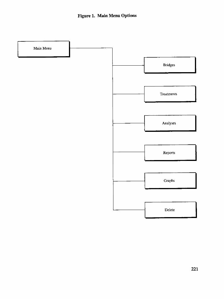
Figure 1. Main Menu Options
Main Menu
Bridges
Treatments
Analyses
Reports [
Graphs
Delete
221

2.3 Quick Tour
The main menu allows considerable flexibility in building, analyzing, and reporting a life-cycle cost analysis of different bridge deck treatments for corrosion. A typical (but by nomeans the only) order in which the main menu items can be accessed is given below.You should not feel confined by this example, however; more general rules on how toproceed through the main menu are given later.
A typical sequence of main menu selections might proceed as follows:
• First, complete the description of a bridge structure in the BRIDGESblock.
• Second, define one or more treatments in the TREATMENTS portion ofthe menu.
• Third, run a corrosion analysis in the ANALYSES portion of the menu. Ifdesired, obtain a corrosion-related report afterward by calling up theREPORTS menu.
• Following the corrosion analysis, run a life-cycle cost analysis of one ormore of the treatments that have been defined, again in the ANALYSESportion of the menu.
• View the results of the life-cycle cost analyses in graphs on the screen,using features provided in the GRAPHS option.
• The graphs may suggest particular reports that would be most useful toobtain and which may be selected in the REPORTS block.
• Results needed for future reference may be retained.. Other files may bedeleted using the DEIJETE options.
This sequence of operations provides a logical order in which to use the features inCORRODE to address a realistic problem. In fact, it is reD' typical of how an agencymight use CORRODE ff it were analyzing a very small number of bridges or looking atbridges one at a time. In other cases, however, more flexibility may be needed -- e.g., toinput information for several bridges at a time, or to describe several treatments at atime. Descriptions of bridges or treatments that were entered previously may need to beupdated with more recent or more accurate information. CORRODE allows theflexibility to approach problems in different ways, subject to the following generalguidelines:
• The BRIDGES and the TREATMENTS options may be entered in anyorder and any number of times. Several bridges may be defined first, thentreatments or vice versa. Data entered previously may be edited at any
222

time. However, a BRIDGE file and a TREATMENT file must becompleted before they are used in any of the ANALYSES.
• To identify which bridge should be studied when specifying a corrosionanalysis or a life-cycle cost analysis in the ANALYSES option, the bridgemust be "selected." Bridge selection is also necessary when definingtreatment files. Bridge selection is made in the BRIDGES option.
• The corrosion analysis of a bridge must be completed prior to a life-cyclecost analysis of that same bridge in the ANALYSES option. The life-cyclecost analysis also requires that you have already selected a bridge foranalysis in BRIDGES and that you have already defined a treatment inTREATMENTS.
• Once both the corrosion and the life-cycle cost analyses are run, you mayrequest displays of these results at any time thereafter, using theREPORTS and the GRAPHS options. Reports and graphs may beobtained at any time, so long as the results files for the particular runs areretained.
• Files that are not to be retained can be deleted using the procedures inDEI _ETE.
As you become more familiar with the system, you will be able to use these guidelines toadvantage. For example, you may begin building a library of information about yourbridge inventory by creating a bridge file for each deck that you may wish to study. Youmay also wish to create a "standard"hypothetical bridge to which you attach "standard"definitions of treatments that can later be copied and tailored to specific decks.Ultimately, you may want to test several treatments at one time so that you maycompare their life-cycle costs and recommended time of performance. All of theseobjectives can be accomplished by using the system's features described in later chapters.
These guidelines provide a general overview of system capabilities and the typical orderof steps that you may follow. Details on each option in the main menu are presented inlater chapters, as follows:
• Chapter 3 discusses bridge descriptions and other capabilities of theBRIDGES options.
• Chapter 4 explains how to define treatments using the TREATMENTSoptions.
• Chapter 5 covers both the corrosion analysis and the life-cycle cost analysisthat are provided in ANALYSES.
• Chapter 6 describes how analysis results may be displayed, using features inREPORTS and GRAPHS.
223
• Chapter 7 covers DELETE and other aspects of file management inCORRODE.
224
3. Bridge Descriptions
3.1 Overview
The description of general bridge characteristics and their selection for data input andanalysis are handled through the BRIDGES option in the main menu. The BRIDGESsubmenu provides three options:
• Selecting a bridge;
• Editing a previously defined bridge file; and
• Creating a new bridge file.
These options are illustrated in Figure 2 and will be explained in more detail below.Following these explanations is a description of the basic information that you may inputto the bridge file.
3.2 Selecting a Bridge
A bridge must be "selected" before its file can be edited or used in any analysisperformed by CORRODE. A bridge must also be selected before other files relating toit (e.g., treatments, reports) can be defined or used, since these data must always beassigned to a specific bridge. In this way, it is always clear to you and to CORRODEwhich file is being edited or applied in an analysis, or to which bridge a file should beassigned.
The name of the selected bridge always appears in the information bar at the bottom ofthe screen, following the "Bridge:" tag. If this name identifies the bridge file you wish towork with, the bridge is already selected and you may proceed. If this name is differentfrom the file you wish to work with, or if you are not sure and would like to check thenames of the bridge files already defined, then choose the SEI.ECT BRIDGE option:
• CORRODE will display the names of currently defined bridges (if any).
• Use the up-down cursor keys to scroll through the list until you find thebridge file name you wish to select.
225

Figure 2. Bridge Menu Options
Bridges
Select Bridge Edit Bridge New Bridge
Bridge Description File
• Name• Comment• Year Constructed
• Deck Area• Traffic
• Capacity• User Cost: Information
226

• Press FIO to complete the selection. The name of the selected bridge filewill appear in the information bar at the bottom of the screen.
3.3 Editing an Existing Bridge File
You may edit an existing bridge file at any time to update information, complete adescription you began earlier, or correct previous errors. However, the CORRODEsystem lets you edit only the currentlyselected bridge file. If the file you wish to edit isnot currently selected, please refer to the preceding section on selecting bridges beforeyou proceed with editing.
Once you have selected the correct bridge file, choose the EDIT BRIDGE option:
• CORRODE will display a blank window. You cannot enter anything inthis window. This feature is to remind you that only the selected bridgecan be edited.
• Press F10 to continue editing, or Escape to quit (for example, if you needto select a different bridge).
• If you pressed F10 above, CORRODE will display the current contents ofthe selected bridge file, which you may then proceed to edit. Explanationsof these data are presented later in this chapter.
• When your editing changes are completed, you may save them by pressingF10. Alternatively, you may press Escape at any time to exit the filewithout saving your most recent changes. (CORRODE will prompt you tobe sure this is your intention.)
3.4 Defining a New Bridge File
You may add to the system's library of bridge files by defining new files. In this way,you can develop a set of files for all reinforced concrete bridge decks in your networkthat you may wish to analyze. To define a new bridge file, select the NEW BRIDGEoption:
• CORRODE will respond with a window in which it asks you for a bridgefile name. In some cases the name of the previously edited file mayalready appear.
• Edit this field to provide the name of the new file, and press F10 tocontinue.
227

• Normally, the name you provide should be different from the names youhave defined previously. If you enter a name that has already beendefined, CORRODE will respond with a message asking, OK to overwriteexisting file? If you respond no (FO, CORRODE will return you to theentry field so that you may modify the name you had entered. If yourespond yes 00, CORRODE will display the current contents of theexisting file you have specified, and the procedure from this point onwardwill be the same as if you had requested to edit an existing file.
3.5 Contents of the Bridge File
The contents of a bridge file are the same regardless of whether you are defining a newfile or editing an existing one. The only difference CORRODE imposes on these twooperations is that when defining a file for the first time, you specify its name; when youare editing an existing file, CORRODE displays the assigned name but does not allowyou to change it. The reason for this feature is that the bridge file name is used as partof the DOS file name for these bridge data as well as for other data files. To maintainorderly file management, CORRODE retains a bridge file name unchanged once it isassigned.
The items within the bridge file are as follows:
• Bridge name: the name that you assign to the bridge file when you firstdefine it. The name is limited to eight alphanumeric characters and mustconform to DOS file-naming conventions. Typically this name relates tothe name of the bridge that is represented.
• Comment: a text field in which you may enter any descriptive information,to a maximum length of 64 characters. This information is not used by theCORRODE system in any way; it is strictly for your convenience. Youmay use this field to describe, for example, more detailed informationabout the bridge deck in question, notes on current deck condition, thedate and findings of the most recent inspection, or comments on the typesof treatments you will be investigating.
• Year (re)constructed: the calendar year in which the deck concrete wasplaced as the result of initial construction or replacement.
• Deck area: the plan area of the bridge deck in square feet.
• Traffic: the two-way traffic volume, vehicles per day or annual-averagedaily traffic (AADT), through the analysis period. If traffic growth ordecline is anticipated, enter the estimated average value over time.
228
• Normal capacity: the two-way capacity of the bridge, in vehicles per day orAADT, under normal operating conditions (i.e., with no construction zonesor other temporary restrictions or devices).
• Average crossing time: the average time for a vehicle to cross the bridge,in minutes, accounting for the variation in traffic volumes throughout theday and year. For example, a weighted average of peak and off-peakconditions would suffice.
• User cost coefficient: the coefficient K2in the formula given below,representing average dollars per vehicle (accounting for the mix of vehiclesin the traffic stream).
• User cost exponent: the exponent noin the formula given below,representing the rate of increase of user costs with deteriorating conditionof the bridge deck.
The user cost function for normal bridge conditions (i.e., in the absence of constructionwork zones or detours) is as follows:
U = K2 {S / S.,}*0 (Eq. 3.1)
where
U = the incremental increase in user costs due to worsening deck condition, indollars per vehicle, computed by CORRODE
K2 = the unit user cost, in dollars per vehicle, that you input above
S = the bridge condition over time that will be estimated by CORRODE in thecorrosion and life-cycle cost analyses
S m = a technological maximum value of distress that you input in the ANALYSISsubmenu (Chapter 5)
no = an exponent controlling the growth of user costs with decreasing deckcondition
This user cost identifies one benefit of keeping a bridge deck in good condition. Theuser cost is intended to reflect primarily travel time considerations and the avoidance ofcongestion costs that would otherwise be due to badly deteriorated decks. However, ifyou wish this function to represent other components of user costs for which you haveestimates (e.g., vehicle wear and tear, safety-related costs), there is no reason why youcould not include these considerations as well in your determination of the value of theunit user cost, k2, above. If reflecting only travel time, K_ should be based on anestimate of the value of travel time for the traffic stream and the uncongested speed (ortravel time) across the bridge.
229
4. Description of Treatments
4.1 Overview
Treatments are activities performed on the bridge deck to address corrosion-relateddistress. These activities may be either preventive or corrective in nature, and mayencompass different techniques (e.g., portland cement concrete (PCC) patching, overlays,sealers, cathodic protection). As new technologies become available, they may also bedefined as treatments to investigate, for example, their potential cost-effectiveness.
In order to encompass a wide range of treatments, CORRODE adopts a flexible inputformat that asks you to describe the essential characteristics of a treatment -- e.g., itsnominal llfe, costs, the production rate at which it can be installed, and so forth.CORRODE does not ask you, however, to classify the treatment in any way -- e.g., togroup it as an "overlay" or a "sealer," for two reasons:
• Treatments can be defined as a combination of techniques: e.g., patchingof distressed areas plus overlay or sealer applied over the entire deck area.
• As new methods are developed or experimental materials are tried, it maynot be possible to classify them according to conventional techniques.
You must therefore ensure that the treatments specified are appropriate to therespective bridge deck and compatible with its elements and materials. Examples ofcompatibility considerations are given in Tables 1 and 2.
The data that describe a treatment are grouped in treatment files, much as the bridgedescriptions are contained in bridge flies. Procedures to create and edit treatment filesare likewise similar to those for bridge files. The organization of treatment input optionsis illustrated in Figure 3. The following sections describe the options available in theTREATMENT submenu and the data contained in each treatment file.
The TREATMENT menu provides three options:
• Editing a previously defined treatment file,
• Creating a new treatment file,
231

Table 1. Selection of Compatible De:k Treatment Alternatives
Technical Cone. AC Seal. Cathod. Reason
Disadvantage Over. Memb. Coat. Protect.
Additional dead load Not Not Not Overlays add to dead load2.critical Good Good Good l
Active cracks in cone. Not Not Active cracks reflect throughGood Good3 concrete.
Existing overlay on Not Not 4 Removal of old system resultsdeck Good Good in rough surface5.
Concrete surface Not Rough concrete surfacescaled Good
Existing slotted Not Scarifyingconcrete damagescathod, protect. Good anodes
Existing polymer Not Good Insulated barsinjection repair inconcrete
Electricity not Not Cathodic protection needsavailable Good electricity
Skid resistance Not Skid resistance may decreasecritical Good6
Steep grades and/or Not Concrete may flow after strikecrossfalls GoOd_ off
Sharp skew and/or Not Difficult to pave with concretecurvature Good finishln_ machines
1. When cathodic protection is used with an overlay.2. Unless, an existing overlay (or a layer of the concrete) is removed and replaced.3. When cathodic protection is used with a concrete overlay.4. May be applied on some concrete overlays.5. Rough concrete surface can puncture membranes, unless a smooth concrete surface can be provided
for the new membrane.
6. Exceptions can exist.7. When slump is 4.5 inches (11.4 centimeters) or more.
232

Table 2. Selection of Compatible Structural Treatment Alternatives
Technical Recast. Preplaced Patch Shot- Cathod. ReasonDisadvantage Aggregate crete Protect.
Repair depth Not Not i Concretemore than 2 Good Good consolidationinches and bonding
can be a
problem
Small area repair Not MobilizationGood not justified
Internal Not Concretevibration Good consolidation
problem can be aproblem
Experienced Not Certain skill._contractor not Good requiredavailable
Electricity not Not Cathodicavailable Good Protection need
electridty
Existing polymer Not Insulated barsinjection repair Goodin concrete
1. Shotcrete may be applied in several stages.
233

Figure 3. Treatment Menu Options
T,eatments I
1Edit Treatments New Treatment.,; Copy Treatment
Treatment Description File
• Name
• Comment
• Data Input Forms
Cost and Productivir.y Data
Estimated Life, Effect ofTreatment
Effects on Traffic
Adjustment Factors
234

• Copying a treatment file defined for one bridge to allow you to apply it toanother bridge.
These options are explained in more detail below.
4.2 Editing an Existing Treatment File
You may edit an existing treatment file at any time to update information, complete adescription you began earlier, or correct previous errors. Choose the EDITTREATMENT option in the submenu:
• CORRODE will display the names of currently defined treatments (if any).
• Use the up-down cursor keys to scroll through the list until you find thename of the treatment file you wish to edit. Select the treatment bypressing Enter.
• You may edit the name of the treatment file, as well as other datacontained therein. Editing the name of the file has the same effect ascreating a new file of that name. In this case the treatment file bearing theoriginal name will remain unchanged when you complete your work. (Thisconvention differs from procedures for bridge files in Chapter 3, in whichnames of current files cannot be changed.)
• When your editing changes are completed, you may save them by pressingF10. The name of the selected treatment file will appear in theinformation bar at the bottom of the screen. Alternatively, you may pressEscape at any time to exit the file without saving your most recent changes.(CORRODE will prompt you to be sure this is your intention.)
• Note: Treatments are associated with specific bridges in CORRODE, sincethe data in a treatment file depends at least to some degree on thecharacteristics of the bridge to which it will be applied. When you edit atreatment file, it will be associated with the currently selected bridge. Ifyou wish to edit a treatment associated with a bridge other than the onecurrently selected in the information bar at the bottom of the screen,return to the BRIDGES menu and select the desired bridge before editingthe treatment. (Refer to Chapter 3 on how to "select" a bridge file.)
235

4.3 Defining a New Treatment File
You may add to the system's library of treatment files by defining new files. In this way,you can develop a set of files for relevant treatments to be considered for the inventoryof bridge decks in your network. To define a new treatment file, select the NEWTREATMENT option:
• CORRODE will respond with a window in which it asks you for atreatment file name. In some cases the name of the previously edited filemay already appear.
• Edit this field to provide the name of the new file, and press the F10 keyto continue.
• Normally, the name you provide should be different from the names youhave defined previously. If you enter a name that h:_ already beendefined, CORRODE will respond with a message asking, OK to overwriteexisting file? If you respond no (N), CORRODE will return you to theentry field so that you may modify the name you had entered. If yourespond yes (Y), CORRODE will display the current contents of theexisting file you have specified, and the procedure from this point onwardwill be the same as if you had requested to edit an existing file.
• Note: When you define a new treatment file, just as when you edit anexisting file, it will be associated with the currently selected bridge. If youwish the treatment to be associated with a bridge ot]herthan the onecurrently selected in the information bar at the bottom of the screen,return to the BRIDGES menu and select the desired bridge beforedefining the treatment. (Refer to Chapter 3 on how to "select" a bridgefile.)
4.4 Copying a Treatment File
Many times you may wish to apply a given type of treatment to more than one bridgedeck. Ideally, you would like to be able to define a treatment only once, and then applythat information to any bridge deck for which the treatment may be applicable. Inpractice, however, this time-saving approach cannot be implemented so easily. Thereason is that the information that describes a treatment depends at least to some degreeon the characteristics of the bridge deck in question. For example, the productivity andcosts of a treatment may depend on the area of the deck _nd how many lanes can beclosed at once to perform work. These data also depend on when the estimate is made,since both productivity and cost vary over time as a result of technological advances,evolving legal requirements and standards of good practice., and cost inflation.
236
CORRODE provides a compromise between these two considerations by allowing you tocopy a treatment file defined for one bridge to a new file to be applied to a differentbridge. You may then modify whatever information, if any, needs to be changed toreflect the application of this treatment to the new bridge. In this way, the integrity ofeach bridge-treatment combination is maintained, but you have the flexibility to usepreviously defined treatments to the greatest advantage possible, without having to inputthe treatment descriptions anew for each bridge.
Select the COPY TREATMENT option in the submenu. CORRODE will provide youwith a set of choices in sequence, as follows:
• First, specify the bridge from which you would like to copy the treatment.You might, for example, select a bridge whose location, size, structuralcharacteristics, traffic, etc., match most closely the bridge in question. Oryou might select a bridge for which the estimates of treatment costs,production rates, etc. are, in your opinion, the most current. Perhaps thereis only one other bridge for which this treatment has been definedpreviously. (There is no requirement that you copy any previously definedtreatment B you may elect instead to define a new treatment file fromscratch, using the NEW TREATMENT option rather than COPYTREATMENT. The whole purpose of COPY TREATMENT is to make atime saving approach available to you in defining your set of treatmentsthroughout the bridge network.)
• Next, CORRODE will ask which treatment you wish to copy from thebridge identified above. CORRODE will display a list of these availabletreatments, through which you may scroll using the up-down cursor keys.When you locate the treatment to be copied, press Enter. If you do notsee the treatment that you intended to copy, you may press Escape to exitthis set of submenus and try another approach (e.g., by selecting a differentbridge for which to search the list of treatments, or by editing an existingtreatment, or by defining a new treatment).
• Finally, CORRODE will ask you for the name of the file to which theselected treatment is to be copied. You may use the same name by whichthe treatment was known for the previous bridge, or you may change thisname. Press F10 to complete the copying operation; or you may pressEscape at any time to quit without copying.
Even if you select the same name as used previously, CORRODE will recognizethe new file as a different file, since CORRODE associates treatment files withthe specific bridges for which they are defined. For example, assume thecurrently selected bridge has the name CONCRETE. You wish to copy atreatment file OVERLAY defined previously for the bridge file named BRIDGEto use with bridge file CONCRETE. Using COPY TREATMENT, first select thebridge name BRIDGE, then the treatment name OVERLAY. When CORRODEasks you the name of the file to be copied to, you may select OVERLAY or any
237

other valid name. If you select OVERLAY., CORRODE will recognize that theOVERLAY file associated with CONCRETE is different from the OVERLAYfile associated with bridge BRIDGE. You may therefore edit these two filesindependently of each other from this point on.
• Once a file is copied, you may edit it as you would any other treatmentfile. (Refer to the previous section on editing existing treatment files.)This allowance extends even to the name of the file. If you edit the nameof a treatment file (plus any other data therein), it is as though a new fileof the same name were defined. (CORROI)E may provide you aninformational message on this point, saying that a file originally defined forthe former bridge has been "reassigned" to the latter bridge. This is foryour information only and has no effect on the files in question.)
As an illustration, consider the example above. Assume that you copy theBRIDGE / OVERLAY file into a new file CONCRETE / OVERLAY (wherethe slash denotes a bridge file / treatment file combination). You now edit theCONCRETE / OVERLAY file (since CONCRETE remains the selected bridge),but in so doing you also change its name to OVLY-1. When you are finished,CORRODE will associate two treatment files with bridge file CONCRETE:OVERLAY (which remains the same as when it was copied) and OVLY-1 (whichreflects your editing changes).
4.5 Contents of the Treatment File
The contents of a treatment file are the same regardless of whether you are defining anew file or copying or editing an existing one. The items w_ithinthis file are as follows:
• Treatment name: the name that you assign to the treatment file when youfirst define it or subsequently copy it or edit it. The name is limited toeight alphanumeric characters and must conform to DOS file-namingconventions. Typically, this name is a brief identification of the type oftreatment that is represented. As noted earlier, treatments that areassigned to different bridges may have the same name; CORRODE willstill regard them as different files, since CORRODE associates eachtreatment explicitly with the bridge for which it is defined.
• Comment: a text field in which you may enter any descriptive information,to a maximum length of 64 characters. The CORRODE system does notuse this information in any way; it is strictly for your convenience. Youmay use this field to describe some technical information about thetreatment in question, for notes on current treatment usage, or to identifytreatment combinations represented by this file.
238

• Technical and cost data: the treatment file contains data in four broadcategories, each associated with a separate data input form that isexplained in the sections that follow. These data include (1) costs andproductivities, (2) the estimated nominal life of the repair, (3) the effect ofthe treatment project on traffic flow, and (4) adjustment factors.
• Viewing the data input forms: you may view the data input forms for eachof the sets of technical and cost data by moving the cursor to the respectiveline on the TREATMENT input submenu and pressing any key when thecursor is on the respective "button" for that form. (The "button" isdisplayed as a field with a "Y" in it.) When you complete data input, pressF10 to close a data input form, save any changes you have made, and moveto the next button on the submenu. (Pressing Escape instead will alsoclose the data input form but will not save your changes. CORRODE willreturn you to the same button on the TREATMENT submenu. When youpress any key thereafter, the same data input form will again be displayed.)
• Navigating the data input forms: you may move through the fields of thedata input forms by using the up-down cursor keys or the tab and shift-tabkeys.
The following sections describe the information contained in each of the TREATMENTdata input forms.
Cost and Productivity Data
You will use the first TREATMENT data input form to describe the cost and time (orproductivity) to perform the treatment. Cost and productivity data are organized inparallel lists of cost components and time or productivity components. CORRODE willcompute the total cost and total time required for a treatment as the sum of thecontributions from each of these components. Costs will be tallied as part of the agencycosts to be accounted for in the life-cycle cost analysis. The time required for atreatment will influence the estimate of the duration of traffic disruption, therebyaffecting the incremental user costs during the project period that will also be accountedfor in the life-cycle cost analysis. Data should be entered only for those cost and timecomponents that are deemed relevant to the particular treatment being defined. If costand time components are not relevant, a zero should be entered for both.
The discussion below refers to various measures of bridge deck condition or distress.Technical explanations of these are given in Chapter 5 in the discussion of corrosion andlife-cycle cost analyses.
• Fixed cost and time required: fixed items of the project are those itemswhose time and cost are not a function of the deck area or amount ofdistress to be repaired. The cost is entered as a lump sum, in dollars. The
239

time is entered in days. (Include a time estJxnate only if the activity causesa restriction to the normal flow of traffic across the bridge.) Examples ofitems that can be included here arc'.mobilizaition and setup of trafficcontrols.
• Deck cost and productivity: components of cost and productivity related toany work that will be performed on the total area of the deck: e.g.,placement of a sealer or an overlay over the entire deck area. The unitcost entered here is in dollars per square foot of deck area; theproductivity is expressed in square feet accomplished per day. Forexample, assume a deck area of 4,000 square feet. If an activity has aproductivity of 200 square feet per day, the total time estimated for thisactivity will be 20 days. If the cost is $25.00 per square foot, the total costestimated will be $100,000.
• CL cost and productivity: components of cost and productivity related towork to address only those areas of the deck that are: chloridecontaminated. The unit cost entered here is in dollars per square foot ofchloride-contaminated deck area; the productivity is expressed in terms ofsquare feet per day, applied only to the chloride-contaminated area.CORRODE computes the estimated area of chloride: contamination overtime in the life-cycle cost analysis (Chapter 5).
• DL cost and productivity: components of cost and productivity related towork to address only those areas of the deck that are delaminated(excluding spalls). The unit cost entered here is in dollars per square footof delaminated deck area; the productivity is expressed in terms of squarefeet per day, applied only to the delaminated area. CORRODE computesthe estimated area of delamination over time in the ]fie-cycle cost analysis(Chapter 5).
• SP cost and productivity: components of cost and productivity related towork to address only those areas of the deck that are spaUed. The unitcost entered here is in dollars per square foot of spalled deck area; theproductivity is expressed in terms of square feet per day, applied only tothe spalled area. CORRODE computes the estimated area of spallingover time in the life-cycle cost analysis (Chapter 5).
• Maintenance cost: the average annual cost of maintaining the treatmentinstallation (not the bridge deck itself), in dollars per square foot. (Thisfeature is intended to be applied to treatments like cathodic protection,which may entail periodic maintenance.)
240
Estimated Life and Effect of Repair
You will use the second TREATMENT data input form to describe the effect of thetreatment on bridge condition. Specific data inputs are as follows:
• Effect on chloride, delamination, or spalls: CORRODE provides three"Yes-No" toggle switches by which you indicate the types of distressaffected by the treatment. If you input Yes (Y) for one or more of theseeffects, CORRODE will prompt you for additional information in the nextgroup of items. If you indicate No (N) for any item, CORRODE assumesthat the treatment has no effect on that particular distress component. Ifyou indicate No (N) for all three categories of distress, CORRODEinterprets this treatment as a preventive activity, and will handle it as suchin subsequent analyses.
Note: preventive activities can be applied only before the time of initialcorrosion at the level of the deck rebar. If, in the corrosion analysis,CORRODE determines that you have specified a preventive treatment andthat corrosion has already begun, it will display a message informing you ofthis conflict and suggesting that you either check the corrosion input dataor specify a corrective rather than a preventive treatment.
• CL, DL, and SP following treatment: three separate inputs describing,respectively, the percent of deck area that following repair is chloridecontaminated, delaminated, and spalled. These inputs collectivelyrepresent your best judgment of how the repair affects the condition andfuture performance of the deck. For example, if patching will repair spallsbut will not remove the existing chloride contamination or addressdelaminated areas, you would input zero for "SP following treatment,"indicating that the treatment corrects the current spalling. You would theninput a nonzero value for chloride and delamination following repair,reflecting the likely amounts of these distresses at the time of repair. Forpurposes of this analysis, the percent area of chloride contamination is thatportion of the deck in which the rebar level chloride exceeds 0.035 percentby weight of concrete.
This feature may also be used to reflect the quality of work or the reliability ofthe treatment. For example, if delaminated areas are to be patched, butexperience indicates that only 90 percent of the delaminated areas are reliablydetected at the time of repair, then "DL following treatment" would be input as10 percent rather than zero.
• Nominal life: the estimated life of the treatment, in years, based on yourexperience and judgment. This nominal life establishes an upper bound forCORRODE's assessment of the actual predicted life of the treatment. Theactual prediction will be based on considerations involving the corrosion
241

rate model, which may reduce the estimated life below the value you inputbut will never increase it. If you have no ilfformation on the nominal lifeof the treatment, estimate this value using the methodology developed inthe report for SHRP Project C-103.4
• Corrosion model: the change in the corrosion rate that is effected by thetreatment. These changes are characterized numerically by a "K" factorthat is explained in the next item. Five options are specified for yourselection: (1) the corrosion rate continues 1:oincrease at the same slope asprior to the treatment (K= 1); (2) the corrosion rate continues to increase,but at a lesser slope than prior to the treatment (0<K< 1); (3) thecorrosion rate remains at the Levelthat existed just prior to the treatmentand neither increases nor decreases with time (K=0); (4) the corrosionrate declines somewhat from the level that existed prior to thetreatment (K<O); or (5) the corrosion rate reduces to zero for some periodof time (refer to the "Life with no corrosion" input item below). To a largedegree, this selection depends on the impact of the treatment on thechloride concentration in the concrete and its effect ,an the rebar.
• K factor:, a quantification of the change in corrosion rate indicated by yourselection of a corrosion model above. K is defined as the ratio two slopesin the corrosion rate curve: the ratio of the slope after the treatment tothe slope before the treatment. In some instances CORRODE will set thevalue of K automatically, based on your selection of a model (e.g., for K= 0or K=I). Where a range of K values is implied (i.e., K<O or O<K<I),input a value that represents your best estimate of the effect of thetreatment on the rate of corrosion.
• Life with no corrosion: if corrosion model 5 is selected above, you haveindicated that the corrosion rate reduces to zero. You must also theninput the estimated time, in years, that the deck will experience nocorrosion. This feature is intended for use with techniques like cathodicprotection. (If you selected an option other than number 3 above,CORRODE does not permit you to enter a value in this field.)
Effect on Traffic
Treatments not only affect the condition of the bridge deck; their performance may alsoaffect the traffic using the bridge, particularly if a work zone is established that restrictscapacity or if a detour is necessary. This TREATMENT input form requests informationthat CORRODE will use to assess impacts to users and related increases in user costsdue to a treatment project.
• Traffic impact: the type of impact that will result from the treatment,depending on how you envision the work will be performed. Two options
242
are specified: "congestion" or "detour." (If you anticipate no congestioni.e., if the treatment requires no work zone or other reduction in thebridge's capacity -- select "congestion" and follow the additional instructionsbelow.)
Note that you may investigate different ways of performing treatments: e.g.,dosing one lane at a time, versus dosing a few lanes at the same time, versusdosing the entire bridge. These options can be defined as separate treatments,analyzed, and compared in terms of their relative costs to the agency and tobridge users.
Congestion
If "congestion" is selected above, you will be prompted for the following informationrelating to the congestion formula described below:
• Unit user cost: the cost coefficient (KI in the formula below), expressed indollars per minute per vehicle. This value would be derived from anestimated value of time for the mixed traffic stream on the bridge. (If nocongestion will be caused by the treatment, or if you do not choose tocompute user costs in your analysis, enter zero.)
• Congestion formula coefficient: a calibrating constant (alpha in theformula below).
• Congestion formula exponent: a calibrating constant (beta in the formulabelow), with a value greater than 1.0.
• Capacity during project: the reduced bridge capacity due to imposition ofa work zone, expressed in vehicles per day or annual-average daily traffic(AADT). This value should not exceed the normal capacity for this bridgethat you input in the BRIDGES option. (If the treatment will have noeffect on traffic flow on the bridge, you should make this value equal tothe normal capacity you input in BRIDGES.)
The congestion formula for use during treatment projects in CORRODE is:
o_
u, q- os,.-¢-6) )+m
where
243
UI = the increment in bridge user costs during the project period due tocongestion caused by the treatment work zone, in dollars per vehicle
KI = the value of bridge user time while traveling, expressed in dollars perminute per vehicle, averaged over the daily traffic stream
ot = a constant with a default value of 0.15
tf = the free-flow travel time across the bridge, in minutes
qo = the average two-way traffic volume across the bridge, in vehicles per day
C = the two-way capacity of the bridge during normal (i.e., non-project) periods,in vehicles per day
C_ = the two-way capacity of the bridge during the project period for thetreatment, in vehicles per day (accounting for typical lane closuresthroughout the project and assuming the typical pattern of peak-hour andoff-peak demand)
B = an exponent with a default value of four
D = the total deck area, in square feet
St. = the index of deck area distress at the time of the treatment
P_ = the productivity of the treatment, in square feet per day
M = a fixed time, as for mobilization, in days
This formula estimates incremental user costs due to congestion that will be incurred bythe traffic stream for the duration of the treatment. The degree of congestion issensitive to traffic volume and the relative reduction in capacity due to the treatmentwork zone. The duration of the treatment is a function of the distressed area and the
productivity of the treatment. (This formula simplifies the actual calculation somewhat,since the actual calculation accounts for individual components of distress, as well as foroverall deck treatments, and their respective contributions to overall duration of thetreatment. The basic idea behind these calculations, however, is illustrated in the aboveformula.)
While Eq. 4.1 provides a correct conceptual treatment of congestion, it is anapproximation, since it is based on daily rather than hourly traffic estimates. Calibrationof the constants t_ and/3 should take this fact into account, together with thecharacteristics of the particular bridge and type of project work zone envisioned: e.g.,the number of through lanes, lane width and side friction, whether one-directional ortwo-directional flow is affected, and anticipated degree of congestion. Literature on thevalue of drivers' time and operational characteristics of highway work zones provides
244

information that can help in these estimates. The default values cited above representthe case of restricted, but not heavily congested, flow through a work zone. The defaultvalue of B (4.0000) is based upon regression analyses of curves for such flows developedin a recent FHWA study.9 The default value of ot (0.15) is based on the premise that thevalue of travel time itself varies as a function of the length of delay, and that forincrements of time of less than 5 or 10 minutes' difference, the value of time decreasesto 15 percent or less of nominal value. '° Other values of these constants can be providedfor different situations:
• For situations in which restricted flows may result in delays exceeding 5 to10 minutes, ¢xmay be increased to values of 1.0. to 3.0 or more.
• For situations in which heavy congestion is anticipated (involving significantstop-and-go cycles and attendant delays), the parameters ot and B can befurther adjusted to fit curves for congested flow such as those illustrated inreference 9.
Please refer to references 9 and 10 for examples of curves illustrating these effects.
Note also that you input the data used in Eq. 4.1 at different times, in different files:
• Data related to the bridge itself, but independent of treatments, are inputin BRIDGES: e.g., the deck area and the normal traffic capacity of thebridge.
• Data dependent on the particular treatment specified (as well as on thebridge to which the treatment may be applied) are input inTREATMENTS: e.g., the restricted capacity of the bridge and thetreatment productivity (which may depend upon the type and size of thework zone contemplated).
Detours
If "detour" was selected earlier, you will be prompted for one item of information: theaverage detour time per vehicle, in minutes. This value should reflect the incrementalincrease in travel time caused by the detour, averaged throughout the day to account forvariations in flow and congestion.
Adjustment Factors
Adjustment factors were discussed in the early stages of CORRODE system design as ameans to perform sensitivity analyses automatically. As of now they are notimplemented.
245

5. Analyses
5.1 Overview
CORRODE includes two basic capabilities to help you analyze bridge deck conditionand treatments:
• A corrosion analysis which considers inspection data and observations ofthe bridge deck concrete, estimates key corrosion-related parameters andthe current condition in terms of a distress index, and uses a deteriorationmodel to predict the change in distress index over time.
• A life-cycle cost analysis which considers the deck deterioration modelestimated above, together with predictions of agency costs and bridge usercosts associated with a treatment, to estimate the life-cycle costs of thattreatment. These life-cycle cost estimates yield the optimal time oftreatment performance, when life-cycle costs are at their minimum.
These two analyses are handled as distinct steps in CORRODE, as illustrated inFigure 4. Since a life-cycle cost analysis requires the results of a corrosion analysis, thecorrosion analysis must precede any life-cycle cost run that refers to it. Beyond this basicrule, however, you have considerable flexibility in how you organize your analyses. Youmay run several life-cycle cost analyses based on a corrosion analysis (e.g., to testdifferent treatments). If you receive an error message after a life-cycle analysis thatsuggests going back to the corrosion data, you may do so, make any corrections needed,and then repeat the corrosion analysis and any life-cycle cost analyses that depend on it.
The analyses are selected in the ANALYSES pull-down menu. Details on how toproceed through each analysis are given in the following sections.
5.2 Corrosion Analysis
Note: the corrosion analysis always applies to the "selected" bridge: i.e., the bridgeidentified in the information bar at the bottom of the screen. If the bridge you wish tostudy is not currently selected, go to the BRIDGES option and select the desired bridgebefore proceeding with the corrosion analysis. (Refer to Chapter 3 for how to select abridge.)
247

Figure 4. Analysis Menu Options
Analyses I
Corrosion I
I Corrosion Analysis IFile Selection
Corrosion Input Data
• Analysis Base Year
• Previous Rehabilitation (SeeFigure 5)
• Concrete w/c Ratio
• Concrete Cover Data
• Protective Systems(See Figure 5)
• Survey of Current Present(See Figure 5)
__[ Life=Cycle Costs ]
Life=Cycle Analysis Input Data
• Selection of Corrosion, TreatmentFiles
• Discount Rate
• Maximum Level of Distre,;s
• Results File
248

Corrosion Analysis File Selection
Once you have entered the corrosion analysis submenu, CORRODE prompts you for thenames of two files:
• Start with: choose any previous corrosion file that you may have used forthis bridge which you would like to use as a point of departure in thecurrent analysis. For example, if you performed a corrosion analysis withCORRODE for the selected deck a year ago, and you would now like toupdate those findings, choose the file pertaining to that run. If this is thefirst time you are analyzing a deck, or you don't wish to select any of thepreviously defined files, select the default.
• Results file: the results of the current corrosion analysis will be stored inthe file you identify here. Choose a name that conforms to DOS-namingconventions. If the name you enter matches that of a previously definedcorrosion file, CORRODE will ask you, 'OK to overwrite existing file?' Ifyou respond no (N), CORRODE will return you to the entry field so thatyou may modify the name you had entered. If you respond yes 00,CORRODE will display the current contents of the existing file you havespecified, and the procedure from this point onward will be the same as ifyou were editing the existing file.
The results file will be assigned specifically to the selected bridge. Thus, it is possible tohave corrosion files of the same name assigned to different bridges. CORRODE regardsthese files as separate, independent files and keeps track of which corrosion files areassigned to what bridges. The name of the currently selected corrosion file appears inthe information bar at the bottom of the screen, to the right of the selected bridge file.
Corrosion Input Data
Once file names are chosen, CORRODE displays the input data in the "start with" file.You may edit these data, and the results will be stored in the "results file." The inputdata are as follows:
• Analysis base year: the calendar year for which the corrosion analysisresults will pertain. Generally this would be the current year.
• Maximum distress: enter the maximum level of distress that can occurbefore some remedial work absolutely must be done. This input, referredto as S,, in Part I of this document is intended to provide an absoluteupper bound to the level of distress that will be accepted in the analysisperformed by CORRODE. It is not indicative of a standard or of yourdepartment's practice, nor is it the level at which you think a treatment
249

should be done. Given its intended meaning, a deck will likely be repairedbefore this threshold is reached. CORRODE will restrict the solutionaccording to this maximum: i.e., it will not allow the: deck condition toworsen beyond this threshold, and it will force a treatment at that time.
• Previous rehabilitation: enter Y if the deck:has been previouslyrehabilitated, N if it has not. If your response is yes, a separate input formwill be displayed, as described in a section below. Also, ff yes is entered,CORRODE suppresses certain other data ilLemsin the input form, sincethey will not be needed in the corrosion analysis.
• W/C deck concrete: enter the water-cement ratio of the deck concrete asa decimal fraction.
• Number of cover data: enter the immber of cores taken to determine
thickness of the concrete cover over the rebar. After you enter thisnumber and press Enter, CORRODE displays an input sheet in which youenter each thickness observation, in inches. CORRODE will use thisinformation to compute the mean and standard deviation of the thicknessdistribution and the estimated thickness at the 90 percent confidence limit.When you have finished entering the thickness data, press F10.
• Protective system: indicate (N or Y) whether a protective system has beeninstalled previously for this bridge deck. A protective system significantlyreduces the rate of ingress of chloride ions into concrete. Protectivesystems are limited to those decks that are not critically contaminated withchloride. Sealers, coatings, and polymer overlays are normally thought ofas protective methods. However, hydraulic cement concrete overlays suchas low slump dense, micro-silica, and latex-modified concrete can also beused as protective methods. If your response is Y, a separate input formwill be displayed, as described in a section below. (Refer to the sectionbelow for a list of installed techniques that are included as protectivesystems in CORRODE.)
• Present Condition: indicate (3( or N) whether the data on the deck arefrom a survey of the condition with respect to corrosion. If your responseis Y, a separate input form will be displayed, as described in a sectionbelow.
Three specialized input forms are mentioned above, dealing:with previous deck repair,protective systems, and present condition survey data, respectively. These additionaldata input forms are shown schematically in Figure 5. Details on these are presented inthe sections below.
Note: Several data collection and testing procedures are alluded to in the followingsections. These procedures are summarized in Table 3 and described in Appendix B.
250
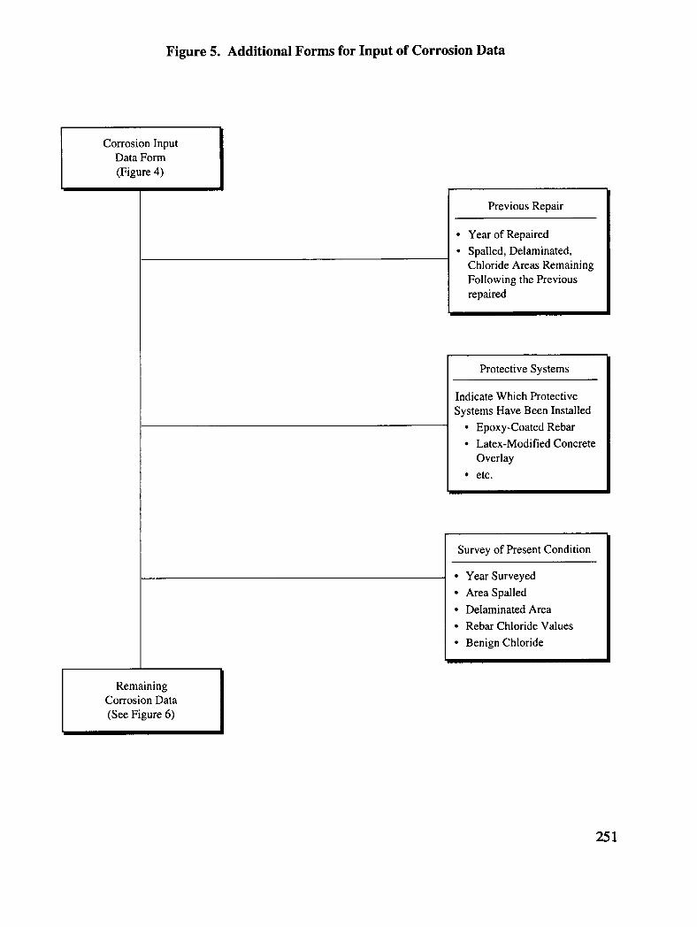
Figure 5. Additional Forms for Input of Corrosion Data
Corrosion InputData Form
(Figure 4)
Previous Repair
• Year of Repaired
• Spalled, Delaminated,Chloride Areas Remaining
Following the Previousrepaired
Protective Systems
Indicate Which Protective
Systems Have Been Installed
• Epoxy-Coated Rebar• Latex-Modified Concrete
Overlay• etc.
Survey of Present Condition
• Year Surveyed
• Area Spalled
• Delaminated Area
• Rebar Chloride Values
• Benign Chloride
RemainingCorrosion Data
(See Figure 6)
251

Table 3. Number of Tests and Samples
Procedure Methodology
Visual Examination Use S-foot grid on deck (2.S-foot grid onsub-and superstructure) to locate defects.
Delamination Survey Use S-foot grid on deck (2.S-foot grid onsub- and superstructure) to locate allareas of delamination. Distinguishbetween delaminations and spalls.
Cover Depth The greater of (1) 40 locations permember or (2)N=40(A/5000) locationsper member, where A-- area in squarefeet of member.
Chloride Profiles The greater of' (1) 10 locations permember or (2) N= 10 (A/5000) locationsper member, where A-- area in squarefeet of member.
Corrosion Potential Use S-foot grid on deck (2.5-foot grid onsub- and superstructure). Additionalmeasurements required to locate sites ofanodic (highest) potential.
Corrosion Rate Measurements at sites of anodiccorrosion potentials; limited to thegreater of (1) 10 locations per member or(2) N= 10(A/5000) locations per member,where A = area in square feet of member.
Concrete Permeability/Resistivity The greater ol' (1) 2 locations per memberor (2) N=2(A/5000) locations permember, where A= area in square feet ofmember.
• One foot is 0_305 meter
• One square foot is 0.093 square meter
252

Previous Repair
When this input form is displayed, enter the following data:
• Year of repair: the calendar year in which the previous repair wasperformed.
• Spalled, delaminated, chloride areas remaining: three separate inputsidentifying the estimated areas of spalling, delamination, and chloride-contaminated areas, respectively, that are estimated to remain followingthe last repair.
• Removal cost: the cost, in dollars per square foot, of removing a previousrepair (e.g., an existing overlay) prior to performing a new treatment. Thisunit cost will be multiplied by the deck area, and the result will be addedto the cost of any treatment. If an existing repair need not be removed, orif removal incurs no additional cost in performing a treatment, enter zero.
When you have completed your entries on this form, exit by pressing F10 to save yourwork and to move to other items on the corrosion data input form. (Pressing Escape willalso exit the form but will return you to the "previous rehabilitation" line on the inputdata form, forcing you to reenter the specialized form until you exit with the F10 key.)
Protective Systems
If you indicate that a protective system is installed, CORRODE displays a list of tensystems from which to make selections. You may select more than one. Indicate yourselections by pressing Enter or Space Bar, both of which operate as a toggle switch.When an item is selected, a small arrowhead pointer appears to the left of the itemnumber on the screen display. In some cases, additional technical information isrequested, as noted below. The ten systems are as follows:
1. Epoxy-coated rebar.
2. Latex-modified concrete overlay.
3. Concrete overlay: enter the thickness of the concrete overlay, in inches, and itswater-cement ratio, as a decimal fraction. These entries may be used for low-slump dense concrete as well. After you have input these values, press F10 tosave the selection of this protective system. If you press Escape, CORRODEwill return you to the list of protective systems, but will not have selected theconcrete overlay.
253
4. Full depth silica fume concrete: enter the rapid permeability test (RPT)coulomb value of the silica fume concrete deck. Exit with F10 to save theselection, or with Escape to ignore it.
5. Silica fume concrete overlay: enter the thickness (inches) and the water-cement ratio (decimal fraction.)of the silica fume overlay. Exit with F10 tosave the selection, or with Escape to ignore it.
6. Asphalt concrete (AC) overlay with waterproof membrane: enter an estimateof the additional years' protection afforded by this protective system. Exit withF10 to save the selection, or Escape to ignore it.
7. Penetrating sealer: enter an estimate of the additional years' protectionafforded by this protective system. Exit with F10 to save the selection, orEscape to ignore it.
8. Surface protective coating: enter an estimate of the additional years'protection afforded by this protective system. Exit with F10 to save theselection, or Escape to ignore it.
9. Corrosion inhibitor concrete: enter an estimate of the additional years'protection afforded by this protective system. Exit with F10 to save theselection, or Escape to ignore it.
10. Other systems: enter an estimate of the additional years' protection affordedby this protective system. Exit with F10 to save the selection, or Escape toignore it.
After you have selected all applicable protective systems, save the list by pressing F10and return to the corrosion input data form. Pressing Escape will also exit the protectivesystems list but will cause CORRODE to ignore any of yore: most recent changes.
Survey of Present Condition
Data from a recent condition survey helps to establish the current condition of thebridge deck and its state of corrosion. CORRODE requires that data from a survey beinput as part of the corrosion analysis. The data are as follows:
• Year surveyed: the calendar year in which the survey was performed.
• Area spalled: the area of the deck exhibiting spalling, in square feet.
• Delaminated area: the area of the deck exhibiting delamination, in squarefeet. Note: this area should not include any of the spaUed area inputabove.
254
• Number of rebar chloride values: enter the number of chloride samplestaken at the level of the reinforcing steel. After you enter this number andpress Enter, CORRODE displays an input sheet in which you enter eachchloride sample value, in percent of total chlorides by weight of concrete.A minimum of 10 rebar level chlorides per 5,000 square feet of decksurface exposed to salty environment (whichever is greater) isrecommended. CORRODE will use this information to compute the meanand standard deviation of the chloride distribution and the estimated rebarlevel chloride at the 90 percent confidence limit. When you are finishedentering the data, press F10.
• Locked in the aggregate: if the information and data available point tochloride-bearing aggregates in the concrete that contribute to corrosion,enter Y; otherwise enter N. If you have entered Y, CORRODE promptsyou for input in the next item of the form, benign chloride.
• Benign chloride: if CORRODE makes this field available, enter theestimated percentage of "benign" chloride (by weight of concrete). Benignchloride refers to chloride locked in the aggregate that will not contributeto corrosion. If previous experience with the aggregate indicates benignchloride, enter the percentage here to modify the threshold chloride valueused in the corrosion analysis.
When you have completed data entry to this input form, press F10 to save these changesor Escape to ignore them.
Analysis: Prior to Start of Deterioration
CORRODE's analysis of the current bridge condition may indicate that corrosion-relateddistress may not yet have begun. CORRODE must still estimate the slope of thedeterioration versus time curve that will occur after corrosion becomes active in thefuture. At this future time, chloride will be present in excess at the level of reinforcingsteel: the corrosion and deterioration rates will be dictated by many factors, includingthe steel concentration, oxygen availability, and resistivity of the concrete in the field. IfCORRODE requires the information needed to estimate the rate of corrosion distress inthe future, it will display a data input form entitled "Pre-Deterioration," as illustrated inFigure 6. (If this form is not displayed, you may skip this section.)
AverageWet Resistivity
The factors that will affect future corrosion cannot be known completely. However, anestimate of whether the deterioration rate will be low, medium, or high should bepossible, and standard curves can be assigned to each rate designation. This estimatecan be based on the wet resistivity input as follows:
255

Figure 6. Remaining Corrosion Data
|Corrosion Data Input |
C';ee Figure 5) I
CORRODE Analyzes Data
Already Input to AnswerQuestion:
Has Corrosion Already
Begun?
No 1 I Yes
Pre-Deterioration Input Post-Deterioration Input
• Average Wet Resistivity • Estimated Start of Corrosion
• Surface Chloride Data • Surface Chloride Data
256

• Average wet resistivity: enter the average wet resistivity of the concrete, inohm-cm. See Appendix B for the method to determine wet resistivity.
CORRODE translates this resistivity into a rate of deterioration as follows: less than7,500 ohm-cm, high; between 7,500 and 30,000 ohm-cm, medium; and greater than30,000 ohm-era is a low rate of deterioration. These results are then translated into theestimated time to reach the maximum level of distress, defining a point needed toestimate the deck deterioration function.
Surface Chloride
Surface chloride levels are part of CORRODE's estimation of future corrosion anddeterioration. Data to be input are as follows:
• Year of surface chloride survey: enter the calendar year in which thissurvey was performed.
• Number of surface chloride values: enter the number of surface chloride
values obtained in the field. After you enter this number and press Enter,CORRODE displays an input sheet in which you enter each surfacechloride data point, in percent by weight of concrete. CORRODE will usethis information to compute the mean and standard deviation of thesurface chloride distribution and the estimated value at the 90 percentconfidence limit. When you have finished entering the surface chloridedata, press F10.
• Mean annual snowfall: enter the mean annual snowfall, in inches. Thismeasure is used as a surrogate for salt applications on the bridge deck. Itis applied only if CORRODE determines that the current surface chloridevalues are extremely low (average less than 0.1 percent by weight ofconcrete) because of lack of exposure age and that the estimate of thefuture time to deterioration (ta) may therefore be incorrect. In that case,the annual snowfall will be used (with other factors) to adjust the estimatedvalue of time to deterioration.
• Exposed to a marine environment: indicate (Y or N) whether the deck isexposed to a marine environment. If your response is Y, CORRODE asksyou further whether the deck is within 25 feet of seawater, to which youagain respond either Y or N. If your first response (on exposure toseawater) was N, then the second question is suppressed by CORRODE.These inputs are applied only if CORRODE determines that the currentsurface chloride values are extremely low (average less than 0.1 percent byweight of concrete) because of lack of exposure age, and that the estimateof the future time to deterioration (ta) may therefore be incorrect. In that
257

case, the degree of exposure to seawater will be used (with other factors)to adjust the estimated value of time to deterioration.
Analysis: After the Onset of Corrosion
CORRODE's analysis of the current bridge condition may indicate that corrosion-relateddistress may have already begun. To estimate the slope of the deterioration versus timecurve, CORRODE must have some information about when corrosion-related distressbegan. If this information is needed, CORRODE will display a data input form entitled"Post-Deterioration," as illustrated in Figure 6. (If this form is not displayed, you mayskip this section.)
Two options are provided to input data on past corrosion, ctepending on whether youalready know the year in which corrosion-related distress _rst occurred:
• Know when corrosion damage started: enter Y or N, depending onwhether you know the year in which corrosion-related distress firstoccurred. Based on your response, CORRODE will prompt you forinformation in certain other fields on the form but suppress the others.
• If so, in what year: if your response above was yes Ctr),enter the year inwhich this distress was first noticed. This year will define the estimatedtime to deterioration, td,of the bridge deck.
• Year of surface chloride survey: if your response above was no (N), dataon the surface chloride level are required to estimate the time todeterioration of this deck. Enter the year this survey was made.
• Number of surface chloride values: enter the number of surface chloridevalues obtained in the survey. At least eight surface chloride levels (0.25to 0.75 inch depth) should be determined per deck or per 5,000 squarefeet, whichever results in the larger number. (These samples should not betaken in patched areas.) After you enter this number, CORRODEdisplays an input sheet in which you enter each surface chloride value, as apercent. CORRODE will use this information to compute the mean andstandard deviation of the surface chloride distribution and the estimatedthickness at the 90 percent confidence limit. When you have finishedentering the surface chloride data, press F10.
Corrosion Analysis Results
When all corrosion data have been entered, CORRODE _!1 perform the corrosionanalysis automatically. (Note: If you think all corrosion data have been entered, but theanalysis has not started, try pressing F10. Either the analysis should begin, or
258
CORRODE will display another corrosion menu or input form for you to complete [e.g.,the pre-deterioration or post-deterioration form].)
Distress Index, S
Note: the following brief description helps to explain the results of the corrosionanalysis. A more complete discussion of the distress index, the corrosion analysis, andthe resulting deterioration function to predict distress over time is given in Part I of thisdocument.
The corrosion analysis results are expressed in terms of a distress index, denoted by S.The distress index is a composite index, a weighted average of several individualcomponents of distress at a given time:
• Percent of rebar level chloride contamination: the percent of deck area inwhich the rebar level chloride contamination exceeds a threshold value of0.035 percent of the weight of concrete.
• Percent delamination: the percent of deck area that is delaminated,excluding spalled areas.
• Percent spalled: the percent of deck area that is spalled.
The weighted averaging formula for the distress index at any time t is as follows:
S = (CL + 2.5 DELAM + 7.5 SPAIJ.) / 8.5, for any time t (Eq. 5.1)
where
S = the distress index, expressed as the weighted average percent of deck areathat is distressed; and
CL = the percentage of deck area that is dfloride contaminated
DELAM = the percentage of deck area that is delaminated
SPALL = the percentage of deck area that is spalled
The distress index is defined on a scale of 0 to 100, with an increasing index valuedenoting increasing distress in the deck. Although the maximum index value ismathematically 100, it is believed that a practiced limit exists, beyond which a functioningdeck should not go without rehabilitation. You input a value for this practical maximumlevel of distress.
259
The corrosion analysis seeks the time variation in the distress index: i.e., a deteriorationfunction, expressed as a logistic or S-shaped curve. To estimate this curve, the corrosionanalysis determines the condition of the deck at key points in its history or future,depending on whether or not the corrosion mechanisms have already begun. These keypoints are ta, the time to the start of deterioration;; tt,,the present time; and t= the timeto reach the maximum level. To estimate the dete.rioration function, the corrosionanalysis requires that only two of these three poinl_sbe determined.
It is assumed that at the time to the start of deterioration, h, the condition index isdefined to have a value of 1.9. This value corresponds to the assumption of 10 percentchloride contamination, 0 percent dclarnination, mad0 percent spalling. Thus, thecorrosion analysis needs only to determine tdto obtain one of the two required points. Itcomputes tdusing a modified Stratfun formula.
For the second point, the corrosion analysis uses one of the following two approaches,depending on whether corrosion has already begun or will begin in the future:
• The current deck condition: Since the present time is known, this
procedure determines the present level of distress Sp.from technicalinformation and the results of field surveys that you input in the corrosionmenu.
• The limiting deck condition: This procedure deterndnes the time at whichthe deck will reach the practical maximum level of distress, estimated fromthe technical data you input in the corrosion menu.
Display of Corrosion Results
Results of the completed corrosion analysis are displayed in a special screen containingthe following information:
• Year of construction" the year of deck construction or replacement thatyou entered in BRIDGES.
• Key points in the distress versus time curve: distress index values at twoof the three possible points are given. These values are based on thepresent condition of the deck if corrosion has already begun, or upon thepredicted future trend of corrosion and related distress if the corrosionmechanism has yet to manifest itself. The possible points are (1) the timeto deterioration, td; (2) the present time, ta,;and (3) the time to reach themaximum distress, t,.
• Deterioration function: expressed as an S-shaped oarve of the followingform: St = 100 / (1 + A exp (-Bt)). This curve is ,derived from fitting alogistic function to two of the three points discussed above.
260
• Time to deterioration: the effective value of h, in years, based on thecorrosion data you have provided.
The life-cycle cost analysis discussed in the next section requires a deck deteriorationfunction estimated by the corrosion analysis. If you wish to save the deteriorationfunction displayed on the results screen for possible future use, press FIO after you havereviewed all of the information on the screen. Press Escape to return to the corrosionanalysis.
5.3 Life-Cycle Cost Analysis
Note: the life-cycle cost analysis always applies to the "selected" bridge, i.e., the bridgewhose file name is identified in the information bar at the bottom of the screen. If the
bridge you wish to study is not currently selected, go to the BRIDGES option and selectthe desired bridge before proceeding with the life-cycle cost analysis. (Refer toChapter 3 for how to select a bridge.)
Life-Cycle Analysis File Selection
Once you have entered the life-cycle cost submenu, CORRODE prompts you for thefollowing information:
• Corrosion analysis file: select the name of the corrosion analysis file to beincluded in the life-cycle cost analysis. This file selection determines thespecific deterioration model to be applied to predict deck distress overtime. Press Enter when finished.
• Treatment definition file: select the name of the treatment file to beincluded in the life-cycle cost analysis. This file selection determines thespecific treatment to be applied, for which the optimal time and cost willbe determined. Press Enter when finished.
• Discounting rate: enter the discount rate, in percent, to be used in theanalysis. Your agency may have already established the value of discountrate to be used in economic analyses of project alternatives. The discountrate at the federal level is set by the Office of Management and Budget. Ifno information on discount rate is available, use the guidance in theAASHTO "Red Book. "t°
• Results file: the results of the current life-cycle cost analysis will be storedin the file you identify here. Choose a name that conforms to DOSnaming conventions. If the name you enter matches that of a previouslydefined life-cycle cost file, CORRODE will ask you, 'OK to overwriteexisting file?" If you respond no (N), CORRODE will return you to the
261

entryfieldsothatyoumay modifythename youhad entered,iffyourespondyes(Y),CORRODE willproceedwiththeaxlalysis-- allpreviouscontents in the results file will be lost.
Life-Cycle Analysis Results
When you have completed data input, press F10. CORRODE will automatically beginthe life-cycle cost analysis. When the analysis is completed., CORRODE will display ascreen entitled, "Life-Cycle Cost Analysis Solution." This screen gives the optimal timeto perform the treatment you had selected earlier for the bridge and the associatedcorrosion model that you also selected.
A message informs you that reports and graphs can be obtadned for this solution,specifying the file name that you should use to obtain these results. The file name is thesame as the "results file" name you specified earlier in the life-cycle analysis menu.When you have finished reading this screen, press any key to return to the CORRODElife-cycle cost submenu.
If the life-cycle cost analysis detects inconsistencies in the bridge, corrosion, andtreatment data that have been specified, it will display a message to that effect. Forexample, if you have input a preventive treatment, but the ,corrosion analysis shows thatcorrosion has already started, CORRODE will display a message pointing to thiscontradiction and suggesting that you either check the corrosion data or describe acorrective rather than a preventive treatment.
262

6. Viewing Results
6.1 Overview
CORRODE provides several ways to view your results of the corrosion and life-cyclecost analyses. Several types of reports and graphs are provided, as described in thefollowing sections. These displays and features are available in the REPORTS and theGRAPHS options of the main menu bar, respectively, as shown in Figure 7.
Note: reports and graphs are available only for the selected bridge: i.e., the bridgewhose file name is displayed in the information bar at the bottom of the screen. If youdesire reports for a bridge other than the one displayed, return to the BRIDGES optionto select a new bridge before proceeding with REPORTS or GRAPHS. (Refer toChapter 3 for selecting bridge file names.)
6.2 Reports
Types of Reports
CORRODE provides you several choices in the REPORTS submenu:
• Corrosion analysis results: a summary of the key data that you haveentered and the results of the corrosion analysis. The informationdisplayed includes the bridge file name, any comment you may haveentered in BRIDGES, general bridge characteristics, results of the surveyof deck distress, rebar chloride values, the current value of the distressindex Sp,estimated points of the deck's distress history, the estimated timeto deterioration td, and the estimated deterioration function S,.
• Life-cycle cost analysis results: a tabulation of the results of a single life-cycle cost analysis for each year, showing the computed agency cost, usercost, and total cost (in thousands of dollars), and identifying the optimaltreatment time (i.e., the year with the lowest life-cycle cost). These resultsapply to a single bridge (the selected bridge) and one treatment; the resultsthat are displayed are retrieved from a single life-cycle cost Kle.
263

Figure 7. Viewing Results
I Reports I
Types of Reports
• Corrosior, AnalysisResults
• Life=Cycle Cost AnalysisResults
• Combined Life=CycleCost Reports
Reports Options
• Create• View
• Print• Delete
Graphs ]
Typ_.._sof Graphs
• Life=Cycle Cost Graph
• Combined Life=Cycle Cost
Graph
264
• Combined life-cycle cost reports: a comparison of the life-cycle cost resultsof several analyses. This report tabulates for each year the computed totalcost (in thousands of dollars) for up to six life-cycle cost analyses. Theoptimal treatment time is identified by an asterisk for each case. Theseresults apply to a single bridge (the selected bridge) and to multipletreatments or variations in treatments, depending on the structure of youranalyses. The results that are displayed are retrieved from multiple life-cycle cost files. Refer to the next section to learn how to choose whichresults will be displayed.
ReportOptions
When you choose one of the three reports above, CORRODE then displays a secondsubmenu from which you select the action you would like to perform. For each type ofreport CORRODE provides the following capabilities:
• Create: generates a report from a file for the first time. CORRODEprompts you for two file names: (1) the name of the file containing thedata to be displayed (select from the list CORRODE provides you); and(2) the name of the file in which the report itself will be stored (enter thisname in the field provided. This name is limited to eight characters andmust conform to DOS-naming conventions.)
• View: displays a report on the screen in tabular form. Select one of thereport file names listed by CORRODE. If no reports have been definedyet for the selected bridge, CORRODE will display a message to thiseffect.
• Print: sends a report file to the printer. CORRODE prompts you for tworesponses: (1) the name of the report file to be printed (select one fromthe list CORRODE provides you); and (2) printer instructions. You mustselect a name of the report file from the list presented. The second fieldmay be left blank.
The CORRODE installation procedure loads the SETUP.PRN file withcommands for an Epson-compatible printer. This set of commands worksreliably with many printers. If you have printer formatting problems whentrying to print reports, try the following:
1. Verify that a file SETUP.PRN exists in the CORRODEsubdirectory. If not, create an empty file of this name, and tryprinting again.
265
2. Copy the current contents of SETUP.PRN to a dummy file; then,erase the contents of SE'RJP.PRN so it is an empty file.(Essentially, you will be invoking your printer's default options.)
3. If the first or second step does not solve the problem, enter anescape command in SETUP.PRN that is appropriate to your printer.Consult your printer manual for the series of corranands required.
These suggestions are intended only for problems in formatting printedreports. If none of these steps solves the problem, review the systemmessages you are receiving to determine whether other causes besidesprinter communications are preventing you from obt_aininga report: e.g.,failure to define a reports file; a different user id or selected bridge fromthat used to create a reports file originally; or inadvertent deletion of areports file.
• Delete: erases a file.
All of the commands above work in a similar way:
• When you must select a file name from a list of previously defined files.CORRODE will always present the correct list of files to you. Forexample, if you are creating a corrosion report, COld.ODE will identifythe list of valid corrosion files. For creating the two life-cycle cost reports,CORRODE will display the valid life-cycle cost fries.
• The combined life-cycle cost report allows you to select a range of files tobe included in a report: a minimum of one file, to a maximum of six. Allvalid life-cycle cost files will be displayed for your selection. If you wish todisplay fewer than six fries, select none for the remaining slots.
• The displayed list of files will always pertain to the selected bridge and thecurrent user id (the three initials entered in the title screen -- seeChapter 2). If you do not find the file name you are: looking for, check tosee that (1) you are currently logged in under the same user id that wasused when the file was created and (2) the currently selected bridge is thesame as that for which the file was created.
• When you are presented with a fist, press Enter to select a name from thelist; press F10 to complete and execute the command, or press Escape tocancel the command and return to the REPORTS submenu.
266

6.3 Graphs
CORRODE displays graphs of life-cycle cost results on the screen. These graphs helpyou visualize a solution and gauge the sensitivity of the life-cycle costs of a treatment tothe timing of its application. They also provide a quick way to compare different life-cycle treatments in terms of their costs versus time. The options presented in thesubmenu correspond to the two types of graphs available:
• Life-cycle cost graph: a graphic display of the life-cycle cost report for asingle treatment discussed in the preceding section. The graph displaysthree cost curves against time in years: agency costs, user costs, and totalcosts. The optimal solution occurs at the point of minimum total cost.
• Combined life-cycle cost graph: a graphic display of the combined life-cycle cost report discussed in the preceding section. The graph displayscurves of total costs versus time in years for up to six different life-cyclecost analyses. This graph is useful to compare different alternativesregarding treatments.
Working with graphs follows the same conventions as discussed for the life-cycle costanalyses and reports, since reports and graphs are derived from the same life-cycleanalysis results files:
• CORRODE will automatically present the valid list of life-cycle cost filesfrom which you may select those to appear in a graph.
• The combined life-cycle cost graph allows you to select a range of files: aminimum of one file, to a maximum of six. All valid life-cycle cost fileswill be displayed for your selection. If you wish to display fewer than sixfiles, select none for the remaining slots.
• The displayed list of files will always pertain to the selected bridge and thecurrent user id (the three initials entered in the title screen -- seeChapter 2). If you do not find the file name you are looking for, check tosee that (1) you are currently logged in under the same user id that wasused when the file was created and (2) the currently selected bridge is thesame as that for which the file was created.
• When you are presented with a list, press Enter to select a name from thelist; press F10 to complete and execute the command, or press Escape tocancel the command and return to the GRAPHS submenu.
There are no file management commands (such as file deletion) associated withGRAPHS, since no permanent files are created. The graphs are generated for screendisplay each time they are needed.
267
7. File Management
7.1 Overview
CORRODE maintains a system of directories and files to help it do its work. Necessarysubdirectories are created during the installation procedure, all located within theCORRODE directory. While these subdirectories and the files therein all follow DOSconventions, you should not attempt to use DOS to work with them. Many of these filescontain not only your data and results but also information that helps CORRODE locatefiles and link information among files. By attempting to access these files through DOS,you may inadvertently change them or delete them in ways that will disable them for useby CORRODE. Messages to the effect that "files are not available" may result if thesefiles are corrupted. (See also the section below, on user id and path conventions.)
All management of files should be done through CORRODE's command structure.Previous chapters have already introduced you to several of CORRODE's filemanagement commands: e.g., creating and editing bridge and treatment files inChapters 3 and 4 (as well as copying treatment files in Chapter 4), the creating ofanalysis files in Chapter 5, and creating and deleting report files in Chapter 6. In thischapter, the remaining file management option will be introduced, the overall DELETEcommand. DELETE is the last option on the main menu bar at the top of the screen.
7.2 The DELETE Option
The DEI.lZ:TE submenu lists four types of files:
• Bridge files: select this option to delete files created in BRIDGES.
• Corrosion files: select this option to delete corrosion files created inANALYSES.
• Treatment files: select this option to delete files created inTREATMENTS.
• Life-cycle files: select this option to delete life-cycle cost files created inANALYSES.
269
These submenu options all operate in a strnilar way:
• Choose the type of file to delete by pressing Enter. CORRODE will listthe names of currently existing files for the ,,;electedbridge that bear yourid (i.e., that are identified by your initials as entered on the title screen).
• To select the name of the file to be deleted, move the cursor to theappropriate name and press Enter. CORRODE will prompt you with amessage confirming that you indeed wish to delete the file. Select Y toproceed with the deletion, or N to quit the operation.
Note: Before deleting a bridge file, please confirm that the bridge is not the "selected"bridge identified in the information bar at the bottom of the screen. Select anotherbridge (using the "Select" command described in Chapter 3) before deleting the bridgefile in question.
270
Appendix A
Input Data Defaults andExample Values
271

Table A.1. Bridge Input Data
Item Default Example
BridgeName Default Example
Comment No Comment An exampleofbridgeinputdata--forillustrationonly
Year(re)constructed 1965 1965
Deckarea,sqft I00 4,000
Traffic,veh/day 100 40,000
Normalcapacity,veh/day 100,000 96,000
Averagecrossingtime,minutes 1 0.02841
Usercostcoefficient,$/veh 0 0.00710
User cost exponent 4.0000 4.0000
272
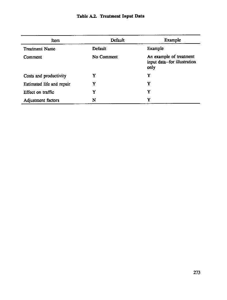
Table A.2. Treatment Input Data
Item Default Example
TreatmentName Default Example
Comment No Comment An example of treatmentinput data--for illustrationonly
Costs and productivity Y Y
Estimated life and repair Y Y
Effect on traffic Y Y
Adjustment factors N Y
273

Table A.3. Treatments: Costs and Productivity Data
Item Default Example
Fixed cost, $ 0 10,000
..time required, days 0 5
Deck cost, $/sq ft 0.00 6.00
..productivity, sq ft/day 0.00 400.00
eL cost, $/sq ft 0.00 0.00
..productivity, sq ft/day 0.00 0.00
DL cost, $/sq ft 0.00 0.0o
..productivity, sq ft/day O.00 0.00
SP cost, $/sq ft 0.00 35.00
..productivity, sq ft/day 0.00 135.00
Maintenance cost, S/year 0 0
274
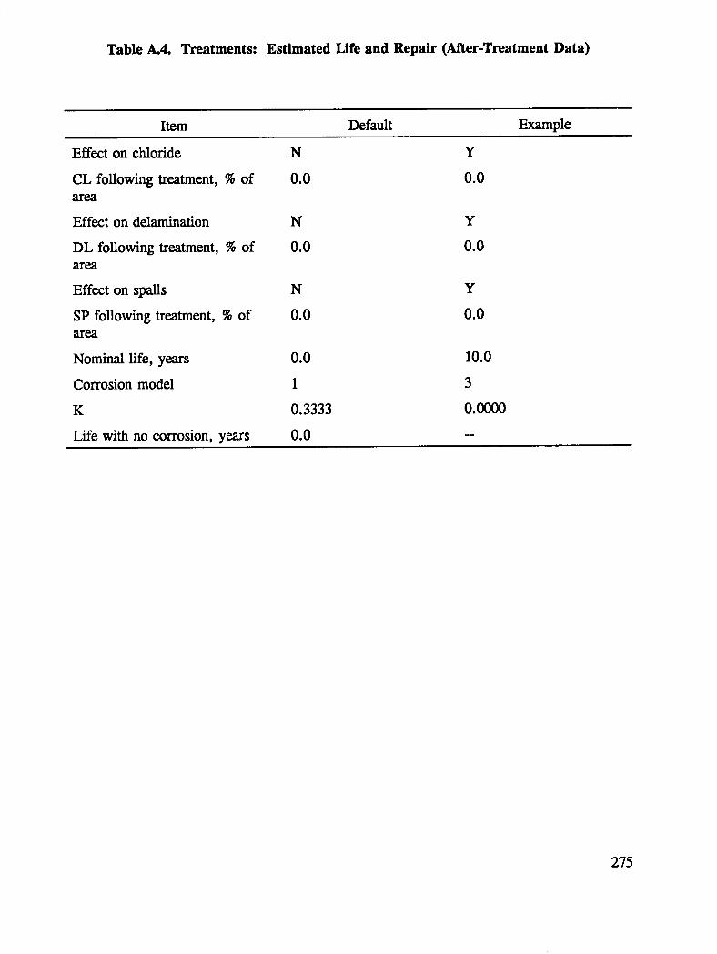
Table A.4. Treatments: Estimated Life and Repair (After-Treatment Data)
Item Default Example
Effect on chloride N Y
CL following treatment, % of 0.0 0.0area
Effect on delamination N Y
DL following treatment, % of 0.0 0.0area
Effect on spalls N Y
SP following treatment, % of 0.0 0.0area
Nominal life, years 0.0 10.0
Corrosion model 1 3
K 0.3333 0.0000
Life with no corrosion, years 0.0 --
275

Table A.5. Treatments: Effect on Traffic
Item Default Example
Traffic Impact Congestion Congestion
Unit user cost, $/min per veh 0.0000 0.25
Congestion formula coefficient 0.1500 0.1500
Congestion formula exponent 4.0000 4.0000
Capacity during project, veh/day 100,000 100,000
Detour time, min/veh 0.00000 --
276
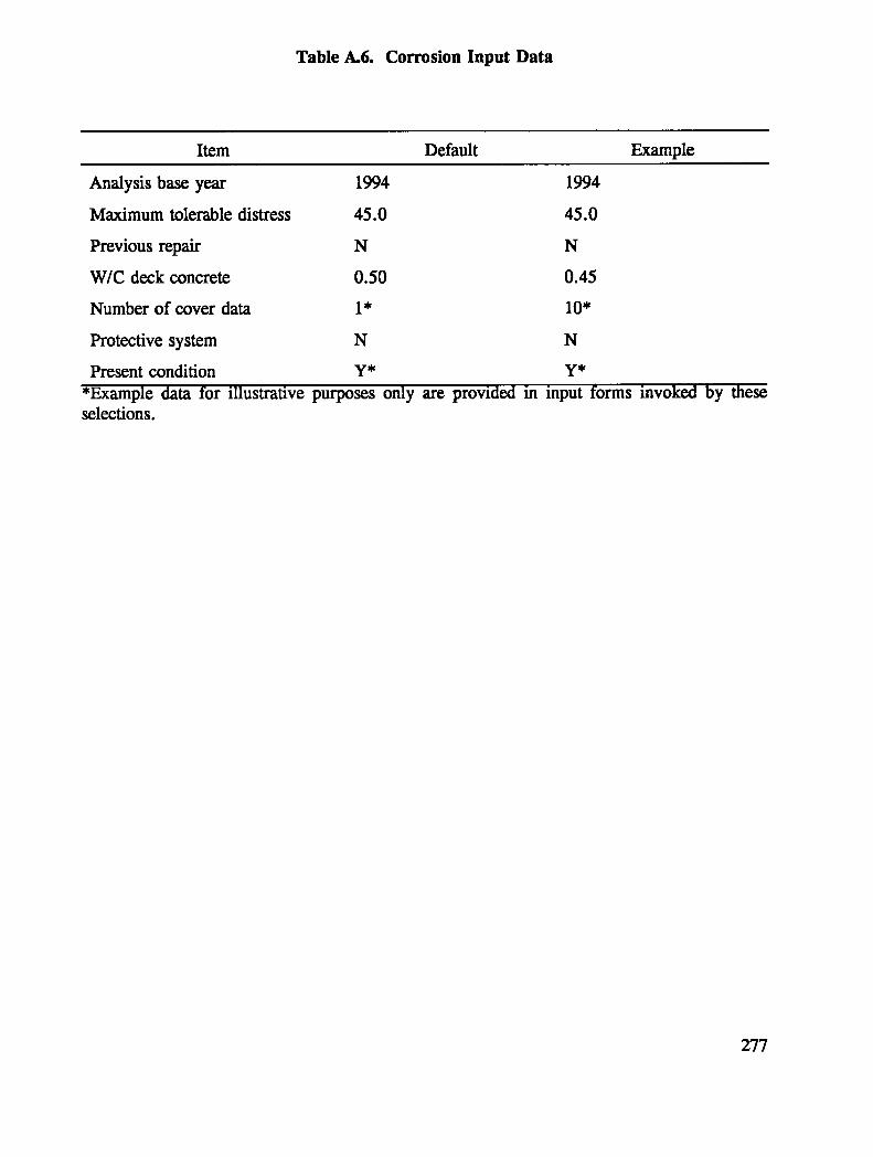
Table A.6. Corrosion Input Data
Item Default Example
Analysis base year 1994 1994
Maximum tolerable distress 45.0 45.0
Previous repair N N
W/C deck concrete 0.50 0.45
Number of cover data 1" 10"
Protective system N N
Present condition Y* Y*
*Example data for illustrative purposes only are provided in input forms invoked by theseselections.
277

Table A.7. Corrosion: Previous Repair Data
Item Default Example
Year of repair 1975
Spalled area remaining, sq ft 0
Delaminated area remaining, sq 0ft
Chloride area remaining, sq ft 0
Removal cost, $/sq ft 0Note: data in this menu not required for the example provided.
278

Table A.8. Corrosion: Present Condition Information
Item Default Example
Year surveyed 1993 1993
Area spalled, sq ft 0 0
Delaminated area, sq ft 0 0
Number of rebar chloride values 1" 10"
Locked in the aggregate N N
Benign chloride, % by weight of 0.00000 --concrete
*Example data for illustrative purposes only are provided in input forms invoked by thisselection.
279

Table A.9. Corrosion: Pre-Deterioration Data
Item Default Example
Average wet resistivity, ohm-cm 1000 500
Year of surface chloride survey 1993 1993
Number of surface chloride 1" 10"values
Mean annual snowfall, inches 0 20
Marine environment N N
Within 25 ft of seawater N --
*Example data for illustrative purposes only are provided in input forms invoked by thisselection.
280

Table A.lO. Corrosion: Post-Deterioration Data
Item Default Example
Know when corrosion damage Nstarted
If so, in what year 1975
Year of surface chloride survey 1993
Number of surface chloride 1"values
*Example data for illustrative purposes only are provided in input form invoked by thisselection.
Note: data in this menunot required for the exampleprovided.
281

Appendix B
Descriptions of Tests
283
APPENDIX B
Descriptions of Tesb;
B.1 Visual Examination
A visual examination of the concrete surface is used 1:odetermine the extent of deteriorationand forms the basis for the subsequentconcrete conditionsurveys. The visual examinationdescribed here is not related to the biennial bridge survey adopted by the Federal HighwayAdministration. The visual examinationnotes both corrosionand non-corrosion-relateddeterioration. It should note size, location, and orientationof
1. Spalls
2. Patches (temporary and permanent)
3. Scaling
4. Pop-outs
5. Cracks
6. Wheeltrack wear
These items should be shown on a sketch. A grid layout is esr_blished on the concretesurface to map concrete deficiencies and to determine their magnitude based on a percent ofsurface area. The severity of the deterioration should be determined quantitatively during avisual examination by measuring the depth of spalls, scaling, and wheeltrack wear. Exposedand corroding reinforcing steel should also be noted.
The visual examination generates a comprehensive condition survey of the concrete surface.It determines the extent of corrosion-induced spalling as well as the significance ofdeterioration caused by reasons other than corrosion of the reinforcing steel. The output ofthis procedure for use in the calculations is the percent of the area which has spalls,temporary patches covering spalls (e.g., asphalt patches), and permanent patches (e.g.,concrete patches).
284
This methodology cannotbe used to determineremedialactions for non-corrosion-relateddeterioration (e.g., scaling, pop-outs, surfacecracking, and wheeltrack wear). If non-corrosion-relateddeterioration is significant, the most cost-effective treatmentmay beobtained by considering factors which are not covered in this methodology.
B.2 Delamination Survey (ASTM D4580)
This test (ASTM D4580) is used to survey concrete by sounding the surface to determine thepresence of delaminations (corrosion-induced internal cracks). To conduct this test, first agrid layout is established on the concrete surface. Second, the surface is sounded anddelaminations noted. Third, the areas of delamination are marked and mapped for thereport. Fourth, the amount of delamination is computed as a percentage of the surface area.Spalls are not included.
Where rigid overlays are applied, ASTM D4580 shall distinguish delaminations fromdebonding of the overlay. Where asphalt concrete overlays are applied, delaminations and/ordebonding should be detected using the procedure recommended by Strategic HighwayResearch Program, _Method for Evaluating the Condition of Asphalt-Covered BridgeDecks." The SHRP test method is documented in Appendix B of SHRP research by Cadyand Gannon.3
If overlay debondlng is significant, the most cost-effective treatment may be obtainedconsidering factors which are not covered in this methodology.
B.3 Cover Depth over Reinforcement Using a Cover Meter (MagneticFlux Device)
This device uses a magnetic field to detect reinforcing steel within hardened concrete. It candetermine the location, orientation, size, and depth of the bar. The accuracy of the device inmeasuring the depth of cover decreases as the depth of cover increases. Magnetic particlesin the concrete can influence the measurements. Thus, a correction factor should be obtained
by exposing the bar at one location and measuring the actual depth. Usually, the correctionfactor is obtained at a location which can later serve as the half cell test bar groundconnection.
If the bar size is not known, the depth cannot be read directly from the scale; therefore, thefollowing technique is suggested.
1. Locate the bar in the test area.
2. Place a two-by-four or other non-metallic spacer between the probe and the concretesurface.
3. Record possible bar size and depth combinations.
285

4. Correct readings for the thickness of the spacerby subtractingits thickness.
5. Place the probe directly on the concrete surface and record possible reading.
Thebarsizeforwhichthesamecoverdepthisobtainedinstepsfourandfiveisthecorrectresult.
B.4 Reinforcing Steel Electrical Continuity
Electricalcontinuity of the reinforcing steel should be;known prior to conducting certain testsor applyingcertain treatments. Electrical continuity can be determinedby measuring theresistancebetween widely separatedsteel components. Low resistivities indicate continuity.
B.5 Chloride Profiles (AASHTO I"260-84, or SHRP Modified TestMethod)
This test determines the chloride content of concrete. Concrete powdered samples arecollected with a vacuum bit near the concrete surface (0.25 to 0.75 inch depth) and at thelevel of the reinforcing steel (the bottom 0.25 inch of concrete cover). Where a concreteoverlay is applied, "concrete surface" is the surface of the oveJqay.
The SHRP "Test Method for Field Determination of Total Chloride Content is documented inAppendix F of Cady and Gannon.3 In the SHRP test method, which is a field method, thepowdered samples are dissolved in, and stabilized by, two solutions. A probe is theninserted into the mixture and the readings are recorded in the field. Calculations convertreadings into chloride content expressed as a percentage of concrete weight.
AASHTO T260-84 test method may also be used for chloride content determination.
B.6 Corrosion Potential Survey (ASTM C876)
This procedure (ASTM C876) determines the potential for the existence of reinforcing steelcorrosion by measuring the electrical potential of the reinforcing steel. It may be performedif 10 percent of the chloride samples at the depth of the steel are greater than the corrosionthreshold chloride content.
The procedure for administering this test follows:
1. Establish a grid on the concrete surface.
2. Provide an electrical connection to the steel (ground).
3. Place a half cell corrosion detection device on the concrete surface at the grid points.
286
4. Record the electrical potential readings.
Note that the test cannot be conducted in the absence of the electrical continuity of thereinforcing steel.
This procedure obtains the location of highest half cell potentials (peak negative potentials)for the subsequent rate of corrosion testing. The location of highest potentialscan beobtained in the field by scanning the concretesurface around the anodic areas with a half celldevice. The locations of anodic areas are obtained by plotting the grid half cell potentialsand drawing equipotential contour lines.
The corrosion potential survey is not recommended for epoxy-coated or galvanized rein-forcement. This is because epoxy-coated bars are electrically insulated from each other, andreadings on galvanized bars indicate the potential of the zinc coating. Also, the test cannotbe conducted where concrete is overlaid with a dielectric material, such as a membrane,polymer material, or asphalt, unless the asphalt is saturated.
B.7 Rate of Corrosion Measurement
The SHRP Standard Test Method for Measuring Instantaneous Corrosion Rate of ReinforcingSteel is documented in Appendix A of Cady and Gannon. 3 The test should be conducted atlocations of highest corrosion potentials (peak negative values) subsequent to the half ceiltest. Corrosion rate tests should not be carded out where epoxy-coated or galvanizedreinforcement is used.
To conduct this test, first mark the bar location and record the bar size and depth. Thepresence of any lap splices should be noted at the test site. Second, establish an electricalconnection to the reinforcement, and determine the corrosion potential directly over the barof interest. Note that the electrical connection provided for the corrosion potential surveycan be used for this purpose. Third, use one of the three devices listed below to takereadings:
1. The 3LP device by KCC, Inc., U.S.A.
2. NSC device by Nippon Steel Corporation, lapan
3. Gecor Drive by GEOCISA, Spain
Each device determines the polarization potentialof the reinforcing steel. Corrosion currentis calculated from a simple equation and expressed in terms of milli-amperes per square footof reinforcing steel area (mA per sq ft). Note that the three devices listed yield different butrelated results. Values obtained by any of the device may be recalculated into values ofanother devices by using the empirical formulas presented below:
287

log I_ (3LP) = 0.47 + 0.84 log I_ (NSC)log I_ (GECOR) = -0.47 + 0.77 log I_ (NSC)log I_(GECOR) = -0.90 + 0.92 log I_ (3LP)
B.8 Permeability of Concrete, and Concrete Resistivity (ASSHTO T277)
This test (AASHTO "1"277)determinesthe relative permeability of the concrete (or concreteoverlay). Also, the test may be modified to determine the concrete's "wet" resistivity. Asuggested procedure for this purpose is,described in Appendix E of Part I of this document.
Many highway agencies are currentlyusing AASHTO T277 (thapidDetermination of theChioride Permeability of Concrete), which requires coring concrete and conducting alaboratory test. The permeability is indicated by the electrical charge passed through theconcrete. The electrical charge is expressed in terms,of coulumbs, and the concreteelectrical resistivity is expressed in terms of ohm-cm.
288
REFERENCES
1. Clear, K. C. Time-to-Corrosion of Reinforcing Steel in Concrete Slabs, Volume 3. Performance after830 Daily Salt Applications. Report no. FHWA-RD-76-70. Federal Highway Administration, U.S.Department of Transportation, Washington, DC: 1976.
2. Cady, P. D., and R. E. Weyers. "Chloride Penetration and the Deterioration of Concrete BridgeDecks," Cement Concrete and Aggregates, CCAGDP, Vol. 5, No. 2 (Winter 1983), pp. 81-87.
3. Cady, P. D., and E. J. Gannon. Condition Evaluation of Concrete Bridges Relative to ReinforcementCorrosion, Volume 8: Procedure Manual. Report no. SHRP-S-330. Strategic Highway ResearchProgram, National Research Council, Washington, DC: 1992.
4. Weyers, R. E., B. D. Prowell, I. L. A1-Quadi, M. M. Sprinkel, and M. Vorster. Concrete BridgeProtection, Repair, and Rehabilitation Relative to Reinforcement Corrosion: A Methods ApplicationManual. Report no. SHRP-S-360. Strategic Highway Research Program, National Research Council,Washington, DC: 1993.
5. Bennett, J., J. B. Bushman, J. J. Bartholomew, K. C. Clear, R. N. Kamp, and W. J. Swait. Cathodic
Protection of Reinforced Concrete Bridge Elements: A Manual of Practice. Report no. SHRP-S-372.Strategic Highway Research Program, National Research Council, Washington, DC: 1993.
6. Beaton, J. L. and R. F. Stratfull. "Environmental Influence of Corrosion of Reinforcing Steel inConcrete Substructures." Highway Research Record 14. HRB, National Research Council, Washington,DC: 1963, pp 60-78.
7. Spellman, D. L., and R. F. Stratfull. Laboratory Corrosion Test of Steel in Concrete. Interim reportno. M&R 635116-3. California Division of Highways: 1968.
8. Recording and Coding Guide for the Structure Inventory and Appraisal of the Nation's Bridges. FederalHighway Administration, U.S. Department of Transportation: 1979.
9. Construction Costs and Safety Impacts of Work Zone Traffic Control Strategies. Report no. FHWA-RD-89-209. Federal Highway Administration, U.S. Department of Transportation: 1989.
10. A Manual on User Benefit Analysis of Highway and Bus-Transit Improvements. American Associationof State Highway and Transportation Officials, Washington, DC: 1977.
289

Concrete and Structures Advisory Committee
Chairman Liaisons
James J. MurphyNew York Department of Transportation (retired) Theodore R. Ferragut
Federal Highway Administration
Vice ChairmanHoward H. Newlon, Jr. Crawford F. Jeneks
Virginia Transportation Research Council (retired) Transportation Research Board
1 Members Bryant MatherUSAE Waterways Experiment Station
Charles J. Arnold
Michigan Department of Transportation Thomas J. Pasko, Jr.Federal Highway Administration
Donald E. Beuerlein
Koss Construction Co. John L. RiceFederal Aviation Administration
Bernard C. Brown
Iowa Department of Transportation Suneel VanikarFederal Highway Administration
RichardD. GaynorNational Aggregates Association�National Ready Mixed Concrete 11/19/92Association
Expert Task GroupRobert J. Girard
Missouri Highway and Transportation Department lqeal S. Berke
W.R Grace and CompanyDavid L. Gress
University of New Hampshire Ken FryerMissouri Highway and Transportation Department
Gary Lee Hoffman *
Pennsylvania Department of Transportation Tony GarciaFlorida Department of Transportation
Brian B. Hope
Queens University Crawford F. Jencks
Transportation Research BoardCarl E. Locke, Jr.
University of Kansas Theodore H. Karasopoulos
MaineDepartmentof TransportationClellon L. Loveall
Tennessee Department of Transportation James E. Roberts
California Department of TransportationDavid G. Manning
Ontario Ministry of Transportation Arun M. Shirole
New York Department of TransportationRobert G. PackardPortland Cement Association Paul Virmani
Federal Highway AdministrationJames E. Roberts
California Department of Transportation 8/9/93
John M. Scanlon, Jr.
Wiss Janney Elstner Associates
Charles F. Scholer
Purdue University
Lawrence L. Smith
Florida Department of Transportation
John R, Strada
Washington Department of Transportation (retired)