Embed Size (px)
Citation preview
Syracuse University Syracuse University
SURFACE SURFACE
Economics - Faculty Scholarship Maxwell School of Citizenship and Public Affairs
2-2004
Life-Cycle Consumption and the Age-Adjusted Value of Life Life-Cycle Consumption and the Age-Adjusted Value of Life
Thomas J. Kniesner Syracuse University and Institute for the Study of Labor
W. Kip Viscusi Vanderbilt University and National Bureau of Economic Research
James P. Ziliak University of Kentucky
Follow this and additional works at: https://surface.syr.edu/ecn
Part of the Economics Commons
Recommended Citation Recommended Citation Kniesner, Thomas J.; Viscusi, W. Kip; and Ziliak, James P., "Life-Cycle Consumption and the Age-Adjusted Value of Life" (2004). Economics - Faculty Scholarship. 123. https://surface.syr.edu/ecn/123
This Article is brought to you for free and open access by the Maxwell School of Citizenship and Public Affairs at SURFACE. It has been accepted for inclusion in Economics - Faculty Scholarship by an authorized administrator of SURFACE. For more information, please contact [email protected].

ISSN 1045-6333
HARVARD JOHN M. OLIN CENTER FOR LAW, ECONOMICS, AND BUSINESS
LIFE-CYCLE CONSUMPTION AND THE AGE-ADJUSTED VALUE OF LIFE
Thomas J. Kniesner
W. Kip Viscusi James P. Ziliak
Discussion Paper No. 459
02/2004
Harvard Law School Cambridge, MA 02138
This paper can be downloaded without charge from:
The Harvard John M. Olin Discussion Paper Series: http://www.law.harvard.edu/programs/olin_center/
The Social Science Research Network Electronic Paper Collection:
http://ssrn.com/abstract=580761
JEL codes: I10, J17, J28, K00
Life-Cycle Consumption and the Age-Adjusted Value of Life
Thomas J. Kniesner *, W. Kip Viscusi **, and James P. Ziliak ***
Abstract
Our research examines empirically the age pattern of the implicit value of life
revealed from workers’ differential wages and job safety pairings. Although aging
reduces the number of years of life expectancy, aging can affect the value of life through
an effect on planned life-cycle consumption. The elderly could, a priori, have the highest
implicit value of life if there is a life-cycle plan to defer consumption until old age. We
find that largely due to the age pattern of consumption, which is non-constant, the
implicit value of life rises and falls over the lifetime in a way that the value for the elderly
is higher than the average over all ages or for the young. There are important policy
implications of our empirical results. Because there may be age-specific benefits of
programs to save statistical lives, instead of valuing the lives of the elderly at less than
the young, policymakers should more correctly value the lives of the elderly at as much
as twice the young because of relatively greater consumption lost when accidental death
occurs.
__________________________
* Krisher Professor of Economics, Senior Research Associate, Center for Policy Research, Syracuse University, Syracuse, NY e-mail: [email protected]
** John F. Cogan, Jr. Professor of Law and Economics, Harvard Law School, 1575 Massachusetts
Avenue, Cambridge, MA phone: (617) 496-0019 e-mail: [email protected]. *** Carol Martin Gatton Chair in Microeconomics, University of Kentucky, Lexington, KY We wish to thank DeYett Law and Gerron McKnight for research assistance. Viscusi’s research is supported by the Harvard Olin Center for Law, Economics, and Business.

1
Life-Cycle Consumption and the Age-Adjusted Value of Life
Thomas J. Kniesner *, W. Kip Viscusi **, and James P. Ziliak ***
© 2004 Thomas J. Kniesner, W. Kip Viscusi, and James P. Ziliak. All rights reserved.
1. Introduction
How the value of life varies over the life cycle has long been of substantial
theoretical interest. Although the quantity of one’s future expected lifetime diminishes
with age the resources one can allocate toward reducing fatality risks change as well.
With the exception of models based on highly restrictive assumptions the value of life
does not peak at birth and steadily decline, as would be the case based solely on one’s
expected future lifetime. Perhaps the principal insight of the life-cycle models of the
value of life is that the value of life at any given age is highly dependent on the life-cycle
pattern of consumption. Thus, the shape of the age-related value of life trajectory is
governed to a large extent by the life-cycle consumption relationship, which we examine
here empirically.
Despite the strong theoretical linkage between the value of life and consumption,
no study of implicit values of life revealed by market decisions has included consumption
in the empirical framework. Hedonic studies using labor market or product market risks
have abstracted completely from the theoretical dependency of the value of life over the
life cycle and the life-cycle pattern of consumption, creating a potential source of bias.
The discrepancies between the estimated and actual values of life may be especially acute
for examining how the value of life varies with age rather than for estimates focusing on
average estimates for a sample. Perhaps because they ignore consumption, every hedonic
labor market study of age variations in the value of life has yielded the implausible result
2
that the value of life turns negative at some age before retirement.1 Explicitly including
consumption in stated preference assessments of the value of life by age does not arise as
an issue because the survey values are elicited directly, not imputed based on market
tradeoffs. Our research provides the first consumption-dependent estimates of the value
of life using hedonic labor-market data.
Reliable estimates of age-related variations in the value of life are of theoretical
and policy interest. The empirical shape of the life-cycle pattern of consumption and the
life-cycle pattern of the value of life not only provide a test of the life-cycle models of the
value of life but also provide evidence indicative of the particular theoretical regime that
is pertinent. Imperfect markets models and perfect markets models yield quite different
estimates of the time path of the value of life.2 Models in which there are imperfect
markets imply an inverted U-shaped relationship between the value of life and age, while
perfect markets models imply a steadily declining value of life with age. Theoretical
models also yield predictions of life-cycle consumption patterns, which are the
foundation of our study because the value of life is derived by decreasing the individual’s
hazard rate within the context of a life-cycle consumption model. On an empirical basis,
the observed relationship between consumption and age is more consistent with the
trajectory embodied in the imperfect markets case than the flat consumption profile in the
perfect markets models.
For policy purposes, there has been increasing interest in age adjustments to the
value of life for benefit assessment, as exemplified by the evaluation of the
1 For example, the value of life becomes negative at age 42 for the results in Thaler and Rosen (1975) and at 48 for the estimate in Viscusi (1979). Viscusi and Aldy (2003) provide a comprehensive review of value of life studies, all of which imply a negative value of life by age 60. 2 For more details on hedonic pricing under imperfect markets see Lang and Majumbar (2003).
3
Environmental Protection Agency’s Clear Skies initiative. Although U.S. government
agencies routinely use market-based estimates for the value of life to assess the risk
reduction benefits of regulations, available market data are not instructive in making age
adjustments because the estimated values of life are often negative. As a result, policy
evaluations have sometimes coupled market estimates of the overall value of life with
survey estimates of how the values should vary with individual age. The results presented
here will provide more meaningful estimates of the age variation in the value of life using
market data, thus putting the baseline value of life and the age variation on comparable
terms.
In what follows we begin with the canonical theoretical and empirical
specification of a hedonic wage function for fatal work-related injury risk. Even in the
canonical specification the implicit value of life can vary with age through an aging effect
on the wage. We then consider an enriched specification of wage hedonics where the
individual’s market wage function reflects that the willingness of a worker to accept risk
may depend on the planned life-cycle path of consumption, which will be another avenue
for age differences in the value of life. The importance of the consumption channel for
aging effects is that the value of life can be constant, increasing, decreasing, or non-
monotonic with age depending on the age profile of consumption. Our empirical results
are consistent with a value of life that follows an inverted U shape. The age pattern of the
implicit value of life that we find is largely due to the importance of consumption in the
wage equation with the peak of the value of life occurring at about age 50. Our focal
result is robust to the measure of consumption and to controlling for industry and
endogeneity of consumption in the hedonic wage equation we estimate. Our finding that

4
the estimated value of life for the elderly is higher than the average value of life in the
data and also higher than the value of life for the youngest workers in the data is
important for policy, which may use an age-dependent value of life that incorrectly
assumes a monotonic decline with age when valuing a program’s benefits.
2. How Consumption Influences the Value of Life
Most models of labor market tradeoffs regarding the value of statistical life are
single-period analyses. Let the utility associated with bequests be zero, the wage be w,
the probability of not being killed on the job be π, and the utility function when healthy
be V(w), which has the usual shape where Vw > 0 and Vww ≤ 0. A worker selecting from a
market opportunities locus in which the wage is a positive but diminishing function of the
fatality risk will select a wage-risk tradeoff, or an implicit value of life, that is equal to
V(w)/(1 − π)Vw, because all wages in any period are consumed.3 Because von Neumann-
Morgenstern utility functions are unaffected by positive linear transformations, division
by the expected marginal utility of income normalizes the value of life in marginal utility
units, eliminating any effect of the scale of the utility function.
If workers’ risky job decisions were simply a sequence of single-period choices
dependence of the value of life on consumption would be quite simple. The estimated
value of life would track the consumption pattern over time, which rises and then later
falls over the life cycle. High levels of consumption for more experienced workers will
raise the numerator of the value of life given by the wage-risk tradeoff, and the high
consumption levels will also lead to lower marginal utility of income. Thus, for any given
level of job risk, both life-cycle consumption influences boost the implicit value of life, at
3 For more discussion of single-period models, see, among many others, Viscusi (1979) and Rosen (1988).

5
least during the middle age years of high consumption, so that the value of life will not be
a steadily declining function of age.
The substantial theoretical literature on the value of life over the life cycle has
utilized models of optimal consumption decisions over time. Within the context of life-
cycle consumption frameworks, what is the value of the individual’s willingness to pay
for a reduction in the hazard rate and how does this value vary with age? Although
models differ considerably in their overall structure and their predictions regarding the
shape of the value of life-age relationship, they all share a common recognition that the
value of life is a function of consumption, the rate of discount, various probabilistic
terms, and, in some models, the worker’s wage rate.
It is instructive to consider the results in an early contribution by Shepard and
Zeckhauser (1984), which provides approximations of the value of life, as well as the
model by Johansson (2002a, 2002b), who provides exact estimates.4 Each model
considers the willingness to pay for temporary reductions in the hazard rate within the
context of life-cycle consumption models for two extreme cases: no insurance available
and perfect annuities markets. With perfect markets the model implies invariant
consumption levels over the life cycle, whereas if there is no annuity insurance
consumption will display an inverted U-shape pattern.5 Thus, the first role of our
examination of empirical consumption patterns is to provide information on which
insurance market regime is pertinent. As is well documented in the literature and will be
shown to be the case below, the age profile of consumption rises then falls over the life
cycle. Our empirical results are consistent with the types of consumption patterns that
4 Other treatments include Arthur (1981), Johansson (2001), Johannesson, Johansson, and Lofgren (1997), Jones-Lee (1989), and Rosen (1988). 5 See Shepard and Zeckhauser (1984), especially pp. 427–428 and p. 433.
6
have been derived in life-cycle model simulations for the no annuity insurance case and
are inconsistent with the consumption predictions of the perfect insurance models.
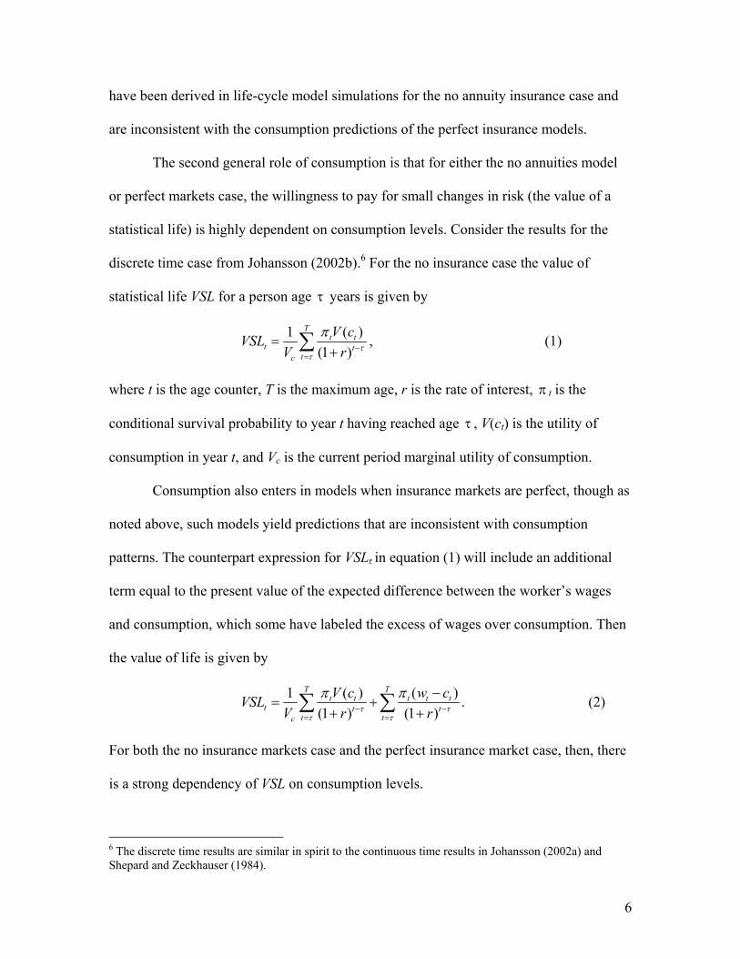
The second general role of consumption is that for either the no annuities model
or perfect markets case, the willingness to pay for small changes in risk (the value of a
statistical life) is highly dependent on consumption levels. Consider the results for the
discrete time case from Johansson (2002b).6 For the no insurance case the value of
statistical life VSL for a person age τ years is given by
( )1(1 )
Tt t
t ttc
V cVSLV r τ
τ
π−
=
=+∑ , (1)
where t is the age counter, T is the maximum age, r is the rate of interest, π t is the
conditional survival probability to year t having reached age τ , V(ct) is the utility of
consumption in year t, and Vc is the current period marginal utility of consumption.
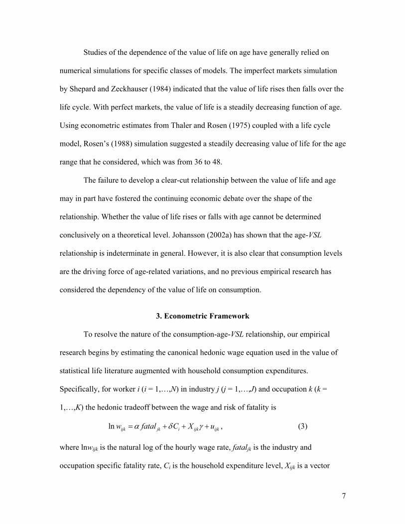
Consumption also enters in models when insurance markets are perfect, though as
noted above, such models yield predictions that are inconsistent with consumption
patterns. The counterpart expression for VSLτ in equation (1) will include an additional
term equal to the present value of the expected difference between the worker’s wages
and consumption, which some have labeled the excess of wages over consumption. Then
the value of life is given by
( ) ( )1(1 ) (1 )
T Tt t t t t
t t tt tc
V c w cVSLV r rτ τ
τ τ
π π− −
= =
−= +
+ +∑ ∑ . (2)
For both the no insurance markets case and the perfect insurance market case, then, there
is a strong dependency of VSL on consumption levels.
6 The discrete time results are similar in spirit to the continuous time results in Johansson (2002a) and Shepard and Zeckhauser (1984).
7
Studies of the dependence of the value of life on age have generally relied on
numerical simulations for specific classes of models. The imperfect markets simulation
by Shepard and Zeckhauser (1984) indicated that the value of life rises then falls over the
life cycle. With perfect markets, the value of life is a steadily decreasing function of age.
Using econometric estimates from Thaler and Rosen (1975) coupled with a life cycle
model, Rosen’s (1988) simulation suggested a steadily decreasing value of life for the age
range that he considered, which was from 36 to 48.
The failure to develop a clear-cut relationship between the value of life and age
may in part have fostered the continuing economic debate over the shape of the
relationship. Whether the value of life rises or falls with age cannot be determined
conclusively on a theoretical level. Johansson (2002a) has shown that the age-VSL
relationship is indeterminate in general. However, it is also clear that consumption levels
are the driving force of age-related variations, and no previous empirical research has
considered the dependency of the value of life on consumption.
3. Econometric Framework
To resolve the nature of the consumption-age-VSL relationship, our empirical
research begins by estimating the canonical hedonic wage equation used in the value of
statistical life literature augmented with household consumption expenditures.
Specifically, for worker i (i = 1,…,N) in industry j (j = 1,…,J) and occupation k (k =
1,…,K) the hedonic tradeoff between the wage and risk of fatality is
ln ijk jk i ijk ijkw fatal C X uα δ γ= + + + , (3)
where lnwijk is the natural log of the hourly wage rate, fataljk is the industry and
occupation specific fatality rate, Ci is the household expenditure level, Xijk is a vector
8
containing a set of dummy variables for the worker’s one-digit occupation (and industry
in some specifications) and region of residence as well as the usual demographic
variables pertaining to worker education, race, marital status, and union status. Finally,
uijk is an error term that admits conditional heteroskedasticity and within fatality risk
autocorrelation.
We begin with the maintained hypothesis that [ | , ] 0ijk jk ijkE u fatal X = , which is
the standard zero conditional mean assumption used in least squares regression.
However, because consumption is a choice variable we expect that [ ] 0ijk iE u C ≠ ; that is,
not only is the zero conditional mean assumption likely violated, but so too is the weaker
zero correlation assumption because of the endogeneity of consumption. This implies we
need an instrumental variables estimator to estimate the model’s parameters consistently.
Selecting an instrument is always a challenge in IV models, but in our case we can rely
on standard results from the theory of the consumer. Specifically, based on human capital
theory we take nonlabor income as having no direct effect on the log wage, but from
static models of consumption and labor supply we take nonlabor income as helping
determine consumption. In other words, if Vi is nonlabor income, then we use for
identification the assumptions that [ | ] 0ijk i iE u V C = and that [ ] 0i iE CV ≠ . Although the
conditional exogeneity of nonlabor income is not testable, the needed covariation of
consumption with nonlabor income is testable via the first-stage regression of Ci on Vi
and the other exogenous variables in the model.

9
Accounting for the fact that fatality risk is per 100,000 workers and that the
typical work-year is about 2000 hours, the estimated value of a statistical life is
^
^ˆ exp(ln ) 2000 100,000ii
wVSL wfatal
α ∂ = = × × × ∂
(4)
where exp(•) is the exponential function and ^
(ln )w is the predicted log wage from the
regression model in (3). The VSL function in (4) can be evaluated at various points in the
wage distribution, but most commonly only the mean effect is reported. In the standard
framework 0δ ≡ in (3) so that age affects VSL only through its direct effect on the wage.
When we allow for 0δ ≠ in (3), changes in the fatality risk implicitly affect both the
wage and consumption levels such that age affects VSL through both a direct effect on the
wage and an indirect effect through consumption (which affects the wage and is itself
age-dependent). We not only report below a distribution of value of statistical life
estimates, but also graphically illustrate the fitted value of life profile over the life cycle.
4. Data and Sample Description
We use two data sources for our research. The first is the 1997 wave of the Panel
Study of Income Dynamics (PSID), which provides individual-level data on wages,
consumption, industry and occupation, and demographics. The PSID survey has followed
a core set of households since 1968 plus newly formed households as members of the
original core have split off into new families. The sample we use consists of male heads
of household between the ages of 18 and 65 who (i) are in the random Survey Research
Center (SRC) portion of the PSID, excludes the oversample of the poor in the Survey of
Economic Opportunity (SEO) as well as the Latino sub-sample, (ii) worked for hourly or
10
salary pay at some point in the previous calendar year, (iii) are not a student, permanently
disabled, or institutionalized, (iv) have an hourly wage greater than $2 per hour and less
than $100 per hour, (v) have annual food expenditures of at least $520 and combined
food and housing expenditures less than $100,000, and (vi) have no missing data on
wages, consumption, education, industry, and occupation. After sample filter (i) there are
2,872 men in the sample, while imposing filters (ii)–(vi) eliminates 997 men such that our
final sample size is 1,875.
The focal variables in our models are the hourly wage rate, consumption
expenditures, and demographics. For workers paid by the hour the survey records the
gross hourly wage rate. The interviewer asks salaried workers how frequently they are
paid, such as weekly, bi-weekly, or monthly. The interviewer then norms a salaried
worker's pay by a fixed number of hours worked depending on the pay period. For
example, salary divided by 40 is the hourly wage rate constructed for a salaried worker
paid weekly. We then take the natural log of the wage rate to minimize the influence of
outliers and to aid in interpreting the model parameters.
A limitation of the PSID relative to the Consumer Expenditure Survey (CE) is the
scope of consumption data. The PSID only records on a regular basis food expenditures
(including food stamps) on food eaten inside and outside the household, as well as
housing expenditures for renters and homeowners with mortgage payments. We consider
two measures of consumption, combined food and housing expenditures and total
consumption. The total consumption measure is based on an imputation method found in
Ziliak (1998). Specifically, he shows that given an estimate of saving, ˆiS , one can derive
an estimate of total consumption as the residual of disposable income and saving,

11
ˆ ˆi i iC Y S= − . Here we estimate saving as ˆ 17,915(0.8169 /1.019) 0.599i iS A= + , where the
inflation adjustment factor on the constant term places the estimate in 1997 dollars and
iA is liquid assets defined as the capitalized value of rent, interest, and dividend income.
For models based on predicted total consumption we impose the additional sample
selection filter that ˆ $1000iC > , which reduces the sample to 1,596 men. Although the
quality of wage data and demographic information in the PSID strongly dominates that
found in the CE, we recognize that our consumption data are less than ideal. It is hoped
that using two separate measures of consumption will offer added robustness. Appendix
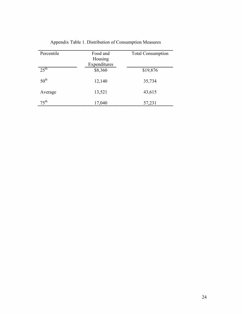
Table 1 provides the sample average and quartile values for consumption.7
The demographic controls in the model include years of formal education, a
quadratic in age, dummy indicators for region of country (northeast, north central, and
west with south the omitted region), race (white = 1), union status (coverage = 1), marital
status (married = 1), and one-digit industry and occupation.
The fatality risk measure used for the analysis is the fatality rate for the worker’s
industry-occupation group. Because published fatality risk measures are available only by
industry, we constructed a worker fatality risk variable using unpublished U.S. Bureau of
Labor Statistics data from the Census of Fatal Occupational Injuries (CFOI).8 The CFOI
provides the most comprehensive inventory to date of all work-related fatalities. The
CFOI data come from reports by the Occupational Safety and Health Administration,
7 It is instructive to note how our estimate of total expenditures aligns with estimates from the CE. Meyer and Sullivan (2003, Table 2) estimate total expenditures for all families with heads 21–62 years of age at the 30th percentile to be $20,314 and at the 50th percentile to be $28,217. Our estimates of total expenditure in Appendix Table 1 are $19,876 at the 25th percentile and $35,734 at the 50th percentile. Our estimates will exceed Meyer and Sullivan’s because we restrict our sample to working prime-age men. 8 The fatality data are available on CD-ROM from the U.S. Bureau of Labor Statistics. The procedure used to construct this variable follows that in Viscusi (2004), who also compares the fatality risk measure to other death risk variables.
12
workers’ compensation reports, death certificates, and medical examiner reports. In each
case there is an examination of the records to determine that the fatality was in fact a job-
related incident. The number of fatalities in each industry-occupation cell is the
numerator of the fatality risk measure.
The denominator used to construct the fatality risk is the number of employees for
that industry-occupation group.9 Workers in agriculture and in the armed forces are
excluded. Because there is less reporting error in the worker industry information than in
worker occupation information, our formulation should lead to less measurement error
than if the worker’s occupation were the primary basis for the matching.10 We
distinguished 720 industry-occupation groups using a breakdown of 72 two-digit SIC
code industries and the 10 one-digit occupational groups. With 6,238 total work-related
deaths in 1997, our procedure created 290 industry-occupation cells with no reported
fatalities.
Because the total number of fatalities was quite stable from 1992 (the first year of
the CFOI data) through our sample year 1997, we used the average annual number of
fatalities for a cell during 1992–1997 when calculating the fatality risk.11 The
intertemporal stability of total fatalities means that the averaging process will reduce the
influence of random fluctuations in fatalities as well as the small sample problems that
arise with respect to many narrowly defined job categories. Using the average fatality rate
9 For the estimate we used the 1997 annual employment averages from the U.S. Bureau of Labor Statistics, Current Population Survey, unpublished table, Table 6, Employed Persons by Detailed Industry and Occupation. For 13 of the 720 categories there was no reported employment for the cell. 10 For further discussion of the measurement error issue, see Mellow and Sider (1983) and Black and Kniesner (2003). 11 For example, in 1992 the total number of fatalities was 6,217, as compared to 6,238 in 1997.
13
from 1992–1997 reduces the total number of industry-occupation cells with no fatalities
to 90 and also makes the fatality risk measure less subject to random events.
The mean fatality risk for the sample is 4/100,000. The range of risk levels by
occupation goes from 0.6/100,000 for administrative support occupations, including
clerical, to 23.5/100,000 for transportation and material moving occupations. The riskiest
industry was mining, with a fatality risk of 24.6/100,000.
5. Wage Equation Estimates
As indicated in (3) above, the basic regression equation we estimate is a semi-log
equation in which the individual worker’s wage is regressed against a series of personal
characteristics, job characteristics, the fatality risk for the worker’s industry-occupation
cell, and consumption. Our regressions explore two different series of specifications. One
set does not include control variables for the worker’s industry and another parallel set of
regressions includes a series of industry control dummy variables defined in terms of
each one-digit industry.
Inclusion of industry control variables potentially can capture omitted industry-
specific differences with respect to job characteristics and market offer curves. However,
here a difficulty arises because the fatality risk variable is constructed using the worker’s
industry as the basis for the matching. Including industry variables will then partly be
inducing multicollinearity with respect to the fatality risk variable. There has been
extensive discussion of the use of industry control variables within the context of
compensating differential research. The consensus is that if the risk variable is
constructed based on the worker’s reported industry then including detailed industry
controls tends to mask the influence of compensating wage differentials for risk rather
14
than reflecting inter-industry wage differentials that may arise apart from risk-related
considerations.12
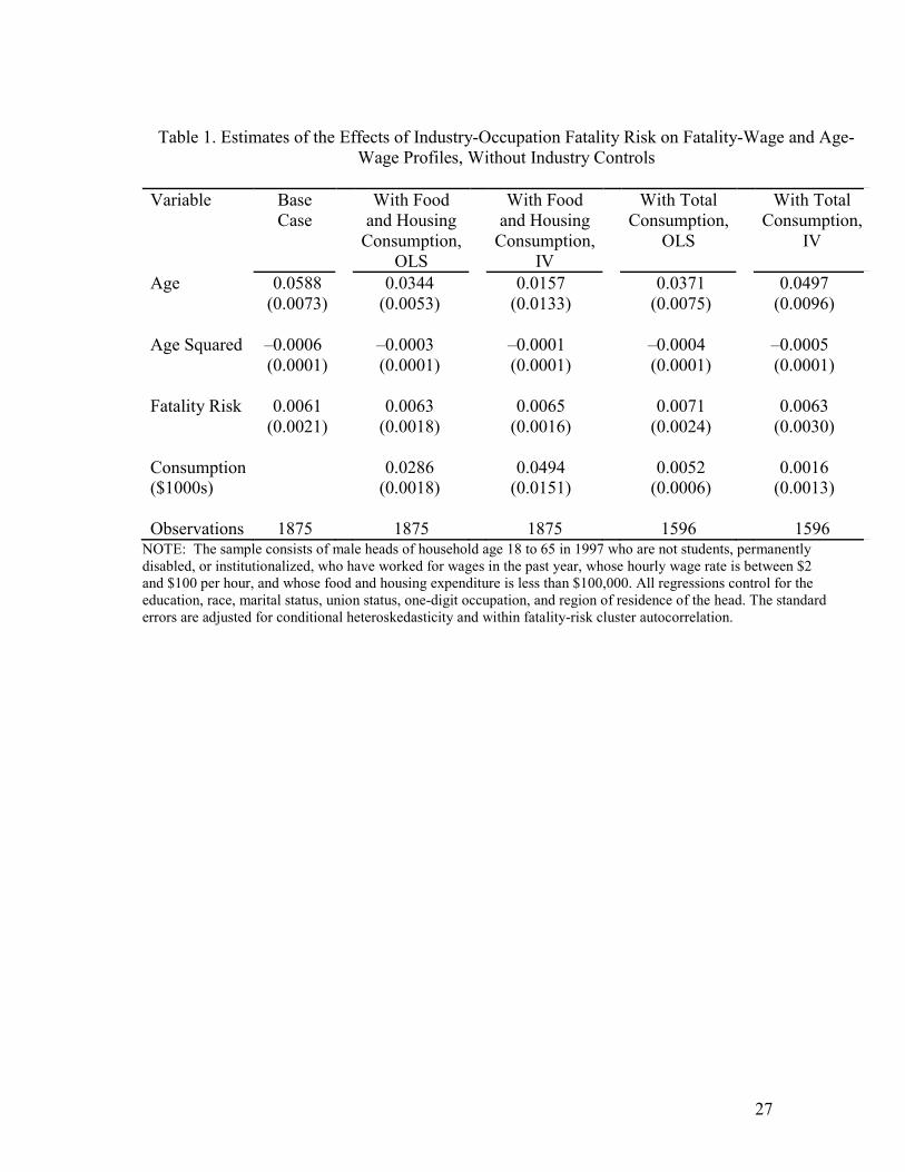
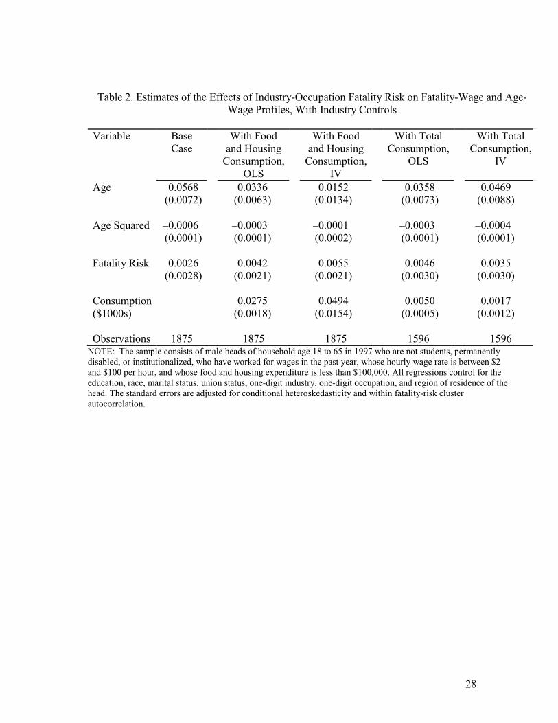
Tables 1 and 2 report the main coefficients of interest, with the standard errors
corrected for conditional heteroskedasticity and for clustering based on the fatality risk
variable. For concreteness, consider first the base case results in each table, where the
estimates do not include consumption and consequently are more comparable to results
found in the literature. Worker wages increase with age, although there is a negative age
squared effect in the baseline estimates. Based on the regression coefficients in Table 1,
the direct effect of worker age is to increase worker wages until age 49 after which there
is a negative influence of age on wages. For the base case excluding the industry controls,
there is evidence of a statistically significant compensating differential for fatality risk,
whereas the fatality risk variable is not statistically significant for the base case in Table
2.
The next set of four equations in each table adds consumption-related variables,
first through ordinary least squares and then using an instrumental variables estimate for
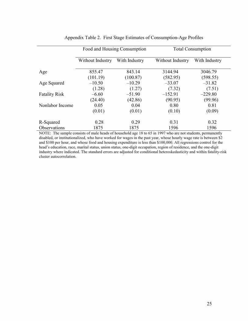
the consumption effect. We record the results of the first-stage consumption regressions
with and without industry controls for our two consumption measures in Appendix Table
2. There is a strong nonlinear effect of age on the level of consumption, and critical for
identification, nonlabor income is an excellent predictor of consumption in all
specifications. The first-stage R2 is about 0.30, and the corresponding F-test is about 29
with a P-value of 0.0000 in each model.
The coefficient of the food and housing consumption variable in the second and
third columns of Tables 1 and 2 is always strongly statistically significant, with 12 For a detailed review of the studies pertaining to this issue, see Section 1 of Viscusi and Aldy (2003).
15
coefficients that are somewhat larger in the instrumental variables estimates than in the
ordinary least squares estimates. The coefficients of total consumption reported in the
final two columns of Tables 1 and 2 also have positive signs, where the effects are
somewhat larger for the OLS results than for the instrumental variables results. In each
instance the IV total consumption coefficient is not statistically significant at the 95
percent level in Table 2.
Including consumption has a much smaller influence on the fatality risk
coefficient for the Table 1 estimates than for the Table 2 estimates. Fatality risk
coefficients range from 0.0061 to 0.0071 for all five specifications in Table 1. In Table 2,
however, inclusion of consumption increases the magnitude of the fatality risk
coefficient. In the case of the food and housing consumption variable, adding
consumption as a regressor in the wage equation boosts the significance of the fatality
risk coefficient so that it becomes statistically significant and at least double the size of
its standard error.
Taking the results of the estimation in conjunction with the characteristics of each
individual worker in the sample we use (4) to calculate a distribution of the value of life
estimates implied by our regression results. The average of the individual values of life in
the base case is $20.9 million for the Table 1 results without industry controls and $8.9
million for the Table 2 results with industry controls. Although the implied values of life
estimates may appear to be high, such results may be a consequence of the particular mix
of workers represented in the Panel Study of Income Dynamics. For example, using
different years and different sample selections, Garen (1988) found estimates of the
16
implicit value of life of $17.3 million using the PSID, while Moore and Viscusi (1990)
generated estimates of $20.8 million using the PSID.
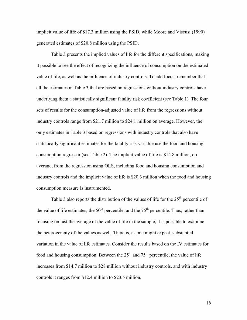
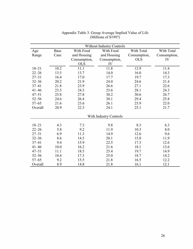
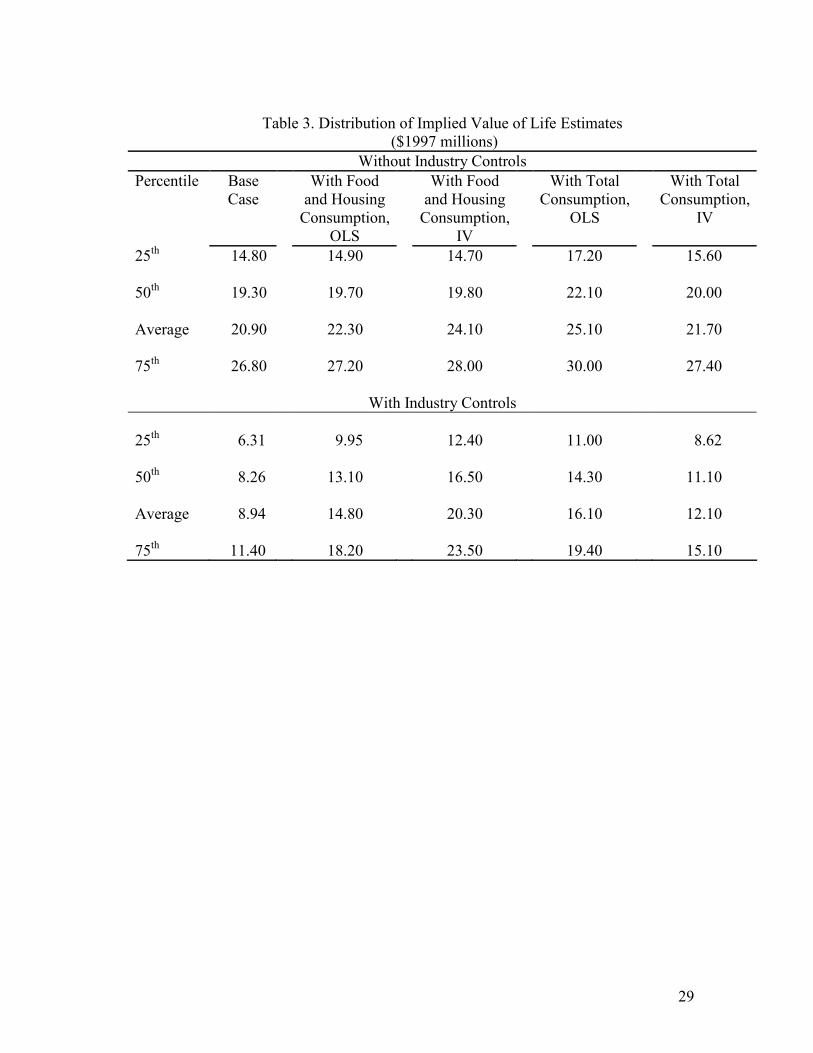
Table 3 presents the implied values of life for the different specifications, making
it possible to see the effect of recognizing the influence of consumption on the estimated
value of life, as well as the influence of industry controls. To add focus, remember that
all the estimates in Table 3 that are based on regressions without industry controls have
underlying them a statistically significant fatality risk coefficient (see Table 1). The four
sets of results for the consumption-adjusted value of life from the regressions without
industry controls range from $21.7 million to $24.1 million on average. However, the
only estimates in Table 3 based on regressions with industry controls that also have
statistically significant estimates for the fatality risk variable use the food and housing
consumption regressor (see Table 2). The implicit value of life is $14.8 million, on
average, from the regression using OLS, including food and housing consumption and
industry controls and the implicit value of life is $20.3 million when the food and housing
consumption measure is instrumented.
Table 3 also reports the distribution of the values of life for the 25th percentile of
the value of life estimates, the 50th percentile, and the 75th percentile. Thus, rather than
focusing on just the average of the value of life in the sample, it is possible to examine
the heterogeneity of the values as well. There is, as one might expect, substantial
variation in the value of life estimates. Consider the results based on the IV estimates for
food and housing consumption. Between the 25th and 75th percentile, the value of life
increases from $14.7 million to $28 million without industry controls, and with industry
controls it ranges from $12.4 million to $23.5 million.
17
6. Age Variations in the Value of Life
An interesting aspect of the heterogeneity of the value of life is the effect of
worker age. The estimates above only reflect the heterogeneity that arises because of
different worker risk levels and differences in worker wages, taking into account that the
overall equation generating the estimates also incorporated differences in individual
consumption. Estimates discussed up to now do not flesh out any systematic difference in
the fatality risk-wage tradeoff that might occur with age. Some studies in the literature
have found age variations in the fatality risk-wage tradeoff, whereas others have not. In
our case, including an age-fatality risk interaction never yielded statistically significant
interaction effects (nor were consumption-fatality risk interactions significant). As a
result, our examination of the life-cycle variations in the value of life will focus on the
effect of age in terms of changes in risk levels, changes in wages over the life cycle, and
the effect of age on consumption based on the consumption-adjusted estimate of the
value of life.
The role of life-cycle consumption is essential to inferring whether there is a
senior discount with respect to the value of life and, if so, how much. Table 4 presents
estimates of the implied value of life for different age ranges within the sample where the
comparisons are relative to the value of life for 18–21 year olds. The results for the base
case without industry controls are illustrative of the following pattern. The value of life
increases to a peak value at age 47–51, which is 2.53 times the value of life of 18–21 year
olds. Then there is a tailing off of the value of life relative to the 47–51 year olds for the
most senior age group in the sample, which consists of workers age 57–65. However,
even for the elderly the value of life is 2.12 times as great as for 18–21 year olds. Indeed,
18
VSL for the oldest group is virtually identical to the relative value of life for 37–41 year
olds (2.13) and even greater than the estimated value of life for all younger workers in the
sample.
Below we consider a series of simulations in which the value of life is calculated
for each worker in the sample using the estimates from Tables 1 and 2 with the worker
specific values of the variables in equation (4). After generating a distribution of implied
values of life for all workers at each individual age in the sample, we then do a
nonparametric estimate (using a cubic smoothing spline with about 180 observations per
band) of the variation in the value of life with age. The nonparametric estimates that
appear in Figures 1–4 enable us to characterize the life-cycle distribution of the value of
life as well as how the distribution is affected by recognition of the role of consumption
in the hedonic wage equation.13
Figures 1a and 1b illustrate the age profiles of VSL for the (no consumption) base
case results without and with industry controls. The figures show a fairly steep rise in the
value of life until a peak at around age 51. The age profile of the implied value of life
based on OLS regression estimates including food and housing consumption in Figures
2a and 2b is considerably flatter than that shown for the no-consumption base case in
Figures 1a and 1b. Recognition of the role of life cycle consumption consequently mutes
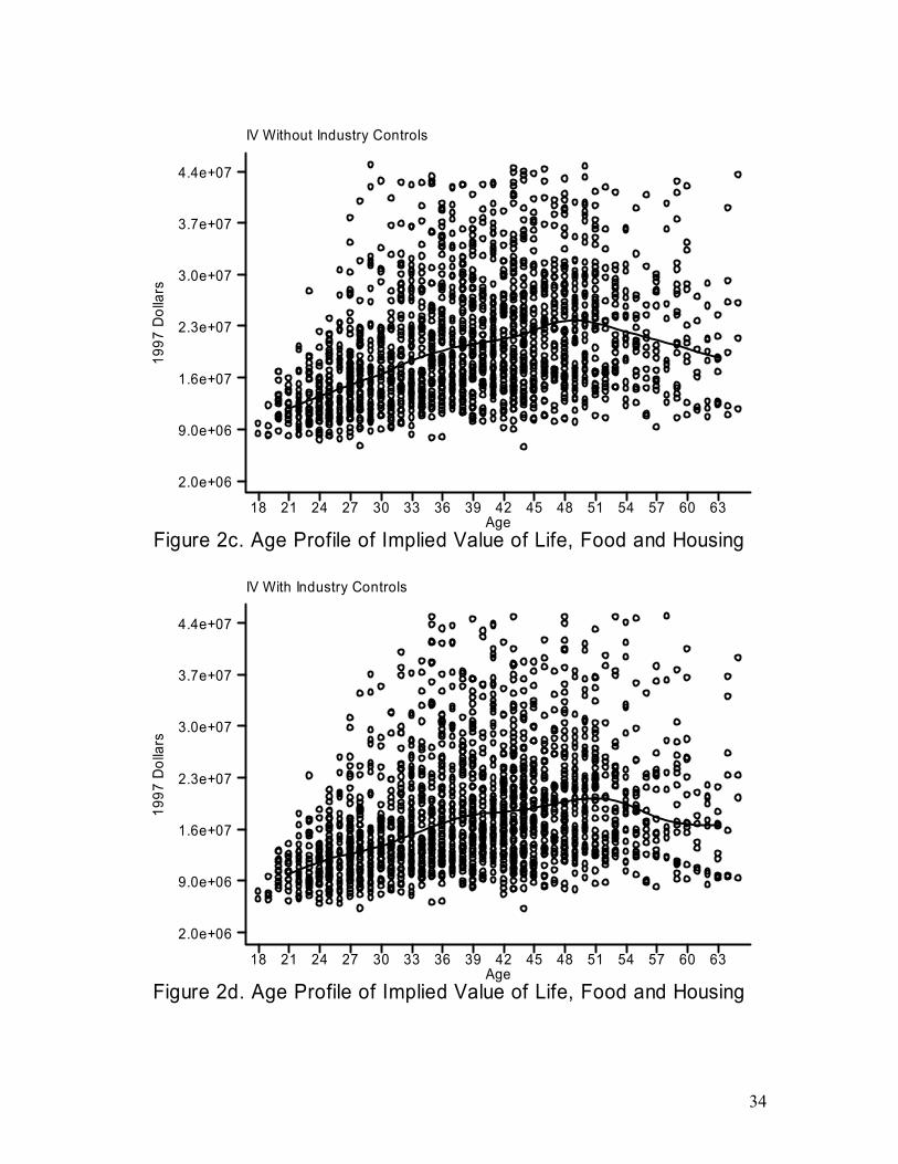
the extent to which there is a life-cycle effect. The results in Figures 2a and 2b, as well as
in Figures 2c and 2d where food and housing consumption has been instrumented,
indicate that the value of life rises with age and declines somewhat, though there is a
flattening of the value beyond age 51 that is less steep than the decline for the base case
where consumption is ignored. 13 Appendix Table 3 also summarizes the numerical values associated with the VSL distribution by age.
19
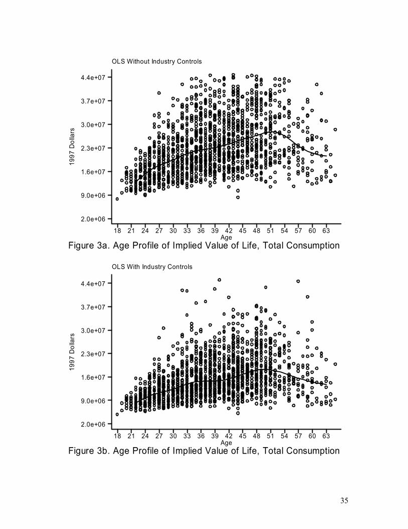
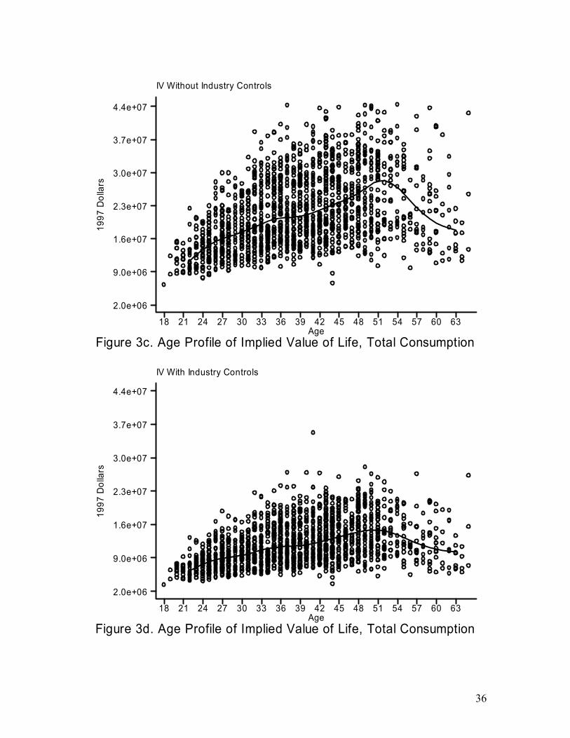
A third set of estimates that are depicted in Figures 3a–3d illustrate how the value
of life varies over the life cycle for models in which actual versus predicted total
consumption is included in the hedonic wage equation with and without industry
controls. The shift to using total consumption has two types of effects in the model with
the most econometric structure, the hedonic wage equation with industry controls and
instrumented total consumption. Note that the decline for seniors is relatively severe in
Figure 3c, more than elsewhere, so our subsequent illustrative example is conservative in
terms of the senior premium. The results reflect a considerable flattening throughout the
age distribution of the value of life, which peaks at $14.9 million, and illustrates the age
distribution of value of life estimates reported in Appendix Table 3 and in the final
column of the bottom panel of Table 4. For the instrumented total consumption hedonic
wage equation case the value of life for 57–65 year olds is 1.94 times the value for 18–21
year olds, and is below the peak multiplicative factor of 2.36 for 47–51 year olds.
On a theoretical basis the estimates for the value of life should be strongly
dependent on individual consumption. For that reason it is instructive to compare the life-
cycle distribution of the estimated values of life with the life-cycle distribution of
consumption. Based on the first-stage consumption estimates in Appendix Table 2,
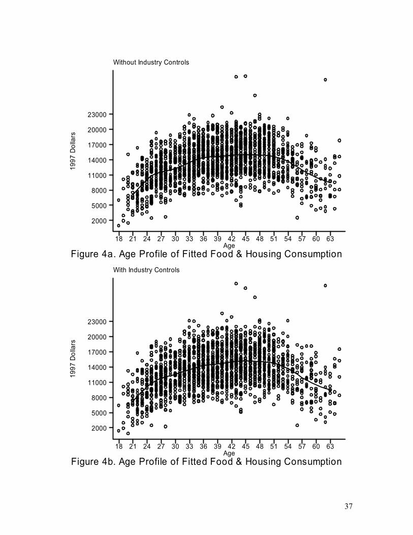
illustrations for two pertinent consumption distributions are the fitted food plus housing
consumption case shown in Figures 4a and 4b and the fitted total consumption
distribution shown in Figures 4c and 4d.
As is indicated in Figures 4a and 4b, consumption of food and housing rises and
then falls over the life cycle. In much the same way, there is an increase and subsequent
decline in the implied value of life, although the decline was not as steep for the value of

20
life in Figures 2b and 2d as the subsequent decline in the nonparametric estimates of the
consumption-age distribution plotted in Figure 4b, for example.
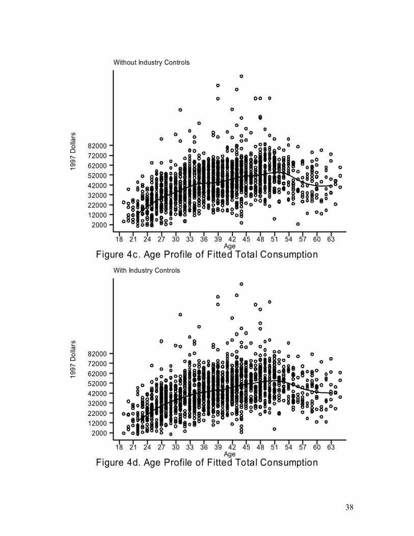
The estimates for the fitted total consumption as a function of age in Figures 4c
and 4d imply that consumption does rise over the life cycle but the decline is much flatter
for the senior age groups than it is for food and housing consumption. In much the same
way as consumption, there is a flattening of the implied value of life curve as a function
of age that was shown in Figure 3d, for example.
The implications of the results concerning the age pattern of consumption are
twofold. First, there is the expected variation in the value of life over the life cycle. The
value of life is not constant but does in fact rise with age, after which it ultimately
declines. However, the decline is not as steep as the earlier increase. Rather, there is a
tendency toward a flattening of the value of life-age relationship. The flattening is
particularly great for models recognizing the dependency of the value of life on total
consumption is recognized. Moreover, the character of the flattening for the value of life-
age profile mirrors a similar shape in the distribution of consumption over the life cycle.
Recognition of the role of life-cycle consumption in estimates of the value of life
consequently illuminates how VSL varies over the life cycle, as a variety of theoretical
models have stressed.
An examination of the life-cycle pattern of consumption for workers indicates that
consumption also is not constant over the life cycle. Rather, it rises and falls, displaying
an inverted U shape that is very similar to the pattern of the value of life in that there is a
flattening at the upper age ranges rather than a decline that mirrors the earlier increase.
The life-cycle consumption pattern is consequently more consistent with the imperfect
21
markets life-cycle consumption models of the value of life rather than the perfect markets
models. The imperfect markets models imply that the value of life will rise and then fall
over the life cycle, which is in fact the pattern in Figures 4a–4d. However, even though
there is a predicted decline in the value of life, the value of life nevertheless is closely
linked to consumption so that there is a flattening of the consumption trajectory for the
more senior age groups. One would also expect a similar flattening of the estimated value
of life, which is in fact reflected in the empirical estimates.
7. Conclusion and Policy Implications
The previous literature has a major disconnect between the theoretical models of
the variations of value of life over the life cycle and market-based estimates of the age
distribution of the value of life. The life-cycle approaches all use a life-cycle
consumption framework in which the value of life is an explicit function of individual
consumption levels. In contrast, no hedonic models of the value of life have ever included
consumption, thus ignoring the fundamental dependency of VSL indirectly through life-
cycle consumption patterns. The neglect of consumption may have been because not only
are consumption data not a usual component of labor market data sets but there is also a
potential endogeneity of the consumption variable.
Our research has provided the first consumption-adjusted estimates of the value of
life, which alter both the value of life estimates as well as their age-related distribution.
Recognizing the dependency on consumption increases the statistical significance and
magnitude of the estimates of the value of life, particularly for estimates including
industry controls. More important are the implications of the consumption-adjusted
values for the life-cycle distribution of the (average) value of life. The value of life rises
22
then falls over the life cycle, but the eventual declines are reasonably flat. The inverted
U-shape pattern of value of life over the life cycle closely follows the time distribution of
consumption shown by the nonparametric estimates of the consumption-age relationship.
The greatest policy interest in the age variation of the value of life stems from the
degree to which there should be a senior discount in the value of life used to evaluate the
benefits associated with regulatory policies that reduce risks to life and health. Our results
show that the implied value of life does decline somewhat for the most senior age group
in the sample. However, even though the VSLs for the elderly are lower than the peak
value of life in middle-age, they are still higher than the values of life for workers age 36
and below.
How our results could affect policy judgments is exemplified by applying the
estimates to the U.S. EPA Clear Skies Initiative, in which the issue of a senior discount
achieved prominence. The first column of Table 5 lists the reduced annual fatalities for a
base case reflecting current scientific knowledge of the effects of long-term exposures
and an alternative case based on risks from short-term exposures.14 Note that the
mortality reduction effects are concentrated among the elderly. The second column
indicates the undiscounted annual benefits in year 2010 for each component monetized
using the EPA’s average value of $6.1 million per life for all lives.15 The mortality
benefits for adults over 65 are $36.6 billion for the base case and $21.9 billion for the
alternative estimates. However, using the 37 percent senior discount advocated in the
controversial U.S. EPA (2002) report, the mortality benefit figure drops to $23.1 billion
14 See the U.S. EPA (2003), Table 16, for the total mortality figures. 15 The $6.1 million per life figure is from the U.S. EPA (2003), p. 26, which is an update of the $6.0 million figure used in U.S. EPA (2002).
23
for the base case and $14.7 billion for the EPA’s alternative estimates.16 If, however, we
use our consumption-adjusted estimates of the relative values of life for the age group
57–65 as the benchmark for assessing values to those 65 and older, the benefit values
increase to $37.1 billion for the base case and $22.3 billion for the alternative case.17 In
contrast, the benefit values for children are half as great using the relative benefit values
for persons age 18–21 to impute an estimate of their value of life. Although the benefit
estimates are meant to be only suggestive, they do indicate how use of a consumption-
adjusted value of life can lead to a significant senior benefit premium rather than a senior
discount.
Framing the valuation question in terms of whether there is a decline in the value
of life with age mischaracterizes the information needs for policy assessments. Standard
policy evaluations use an average value of life for an entire population to assess the
benefits. The pertinent question is whether for the senior age groups there should be a
discount or premium relative to the population average, not with respect to the peak value
of life. Our results shown in Appendix Table 3 for the age 57–65 group indicate that for
every set of estimates the implied value of life for ages 57–65 is somewhat higher than
the overall average for workers of all ages. At least for the pre-retirement age groups we
study, the benefits assessment issue of whether there is a senior discount is in fact a non-
issue.
16 The 37 percent discount figure cited in U.S. EPA (2002), p. 35, is derived from the stated preference survey results in the U.K. by Jones-Lee (1989). 17 The relative value of life estimates in the last column of Table 5 use the statistics from Appendix Table 3, without industry controls, with total consumption, IV.
24
Appendix Table 1. Distribution of Consumption Measures
Percentile
Food and Housing
Expenditures
Total Consumption
25th
$8,360 $19,876
50th
12,140 35,734
Average
13,521 43,615
75th 17,040 57,231
25
Appendix Table 2. First Stage Estimates of Consumption-Age Profiles
Food and Housing Consumption
Total Consumption
Without Industry
With Industry Without Industry With Industry
Age 855.47 (101.19)
843.14 (100.87)
3144.94 (582.95)
3046.79 (598.55)
Age Squared –10.50 (1.28)
–10.29 (1.27)
–33.07 (7.32)
–31.82 (7.51)
Fatality Risk –6.60 (24.40)
–51.90 (42.86)
–152.91 (90.95)
–229.80 (99.96)
Nonlabor Income 0.05 (0.01)
0.04 (0.01)
0.80 (0.10)
0.81 (0.09)
R-Squared 0.28 0.29 0.31 0.32 Observations 1875 1875 1596 1596 NOTE: The sample consists of male heads of household age 18 to 65 in 1997 who are not students, permanently disabled, or institutionalized, who have worked for wages in the past year, whose hourly wage rate is between $2 and $100 per hour, and whose food and housing expenditure is less than $100,000. All regressions control for the head’s education, race, marital status, union status, one-digit occupation, region of residence, and the one-digit industry where indicated. The standard errors are adjusted for conditional heteroskedasticity and within fatality-risk cluster autocorrelation.
26
Appendix Table 3. Group Average Implied Value of Life (Millions of $1997)
Without Industry Controls
Age Range
Base Case
With Food and Housing
Consumption, OLS
With Food and Housing
Consumption, IV
With Total Consumption,
OLS
With Total Consumption,
IV
18–21 10.2 11.1 11.8 12.9 11.4 22–26 13.5 13.7 14.0 16.0 14.3 27–31 16.4 17.0 17.7 19.7 17.3 32–36 20.2 21.9 24.0 24.6 21.4 37–41 21.8 23.9 26.6 27.1 22.6 41–46 23.5 24.3 25.6 28.1 24.3 47–51 25.8 27.8 30.2 30.6 26.7 52–56 24.6 26.4 30.1 29.4 25.8 57–65 21.6 23.6 26.1 25.9 22.0 Overall 20.9 22.3 24.1 25.1 21.7
With Industry Controls 18–21 4.3 7.3 9.8 8.3 6.3 22–26 5.8 9.2 11.9 10.3 8.0 27–31 6.9 11.3 14.9 12.6 9.6 32–36 8.6 14.5 20.1 15.8 11.9 37–41 9.4 15.9 22.5 17.3 12.6 41–46 10.0 16.2 21.6 18.1 13.6 47–51 11.1 18.5 25.4 19.7 14.9 52–56 10.4 17.3 25.0 18.7 14.2 57–65 9.2 15.5 21.8 16.5 12.2 Overall 8.9 14.8 21.8 16.1 12.1
27
Table 1. Estimates of the Effects of Industry-Occupation Fatality Risk on Fatality-Wage and Age-
Wage Profiles, Without Industry Controls
Variable
Base Case
With Food and Housing
Consumption, OLS
With Food and Housing
Consumption, IV
With Total Consumption,
OLS
With Total Consumption,
IV
Age 0.0588 (0.0073)
0.0344 (0.0053)
0.0157 (0.0133)
0.0371 (0.0075)
0.0497 (0.0096)
Age Squared –0.0006 (0.0001)
–0.0003 (0.0001)
–0.0001 (0.0001)
–0.0004 (0.0001)
–0.0005 (0.0001)
Fatality Risk 0.0061 (0.0021)
0.0063 (0.0018)
0.0065 (0.0016)
0.0071 (0.0024)
0.0063 (0.0030)
Consumption ($1000s)
0.0286 (0.0018)
0.0494 (0.0151)
0.0052 (0.0006)
0.0016 (0.0013)
Observations 1875 1875 1875 1596 1596 NOTE: The sample consists of male heads of household age 18 to 65 in 1997 who are not students, permanently disabled, or institutionalized, who have worked for wages in the past year, whose hourly wage rate is between $2 and $100 per hour, and whose food and housing expenditure is less than $100,000. All regressions control for the education, race, marital status, union status, one-digit occupation, and region of residence of the head. The standard errors are adjusted for conditional heteroskedasticity and within fatality-risk cluster autocorrelation.
28
Table 2. Estimates of the Effects of Industry-Occupation Fatality Risk on Fatality-Wage and Age-Wage Profiles, With Industry Controls
Variable
Base Case
With Food and Housing
Consumption, OLS
With Food and Housing
Consumption, IV
With Total Consumption,
OLS
With Total Consumption,
IV
Age 0.0568 (0.0072)
0.0336 (0.0063)
0.0152 (0.0134)
0.0358 (0.0073)
0.0469 (0.0088)
Age Squared –0.0006 (0.0001)
–0.0003 (0.0001)
–0.0001 (0.0002)
–0.0003 (0.0001)
–0.0004 (0.0001)
Fatality Risk 0.0026 (0.0028)
0.0042 (0.0021)
0.0055 (0.0021)
0.0046 (0.0030)
0.0035 (0.0030)
Consumption ($1000s)
0.0275 (0.0018)
0.0494 (0.0154)
0.0050 (0.0005)
0.0017 (0.0012)
Observations 1875 1875 1875 1596 1596 NOTE: The sample consists of male heads of household age 18 to 65 in 1997 who are not students, permanently disabled, or institutionalized, who have worked for wages in the past year, whose hourly wage rate is between $2 and $100 per hour, and whose food and housing expenditure is less than $100,000. All regressions control for the education, race, marital status, union status, one-digit industry, one-digit occupation, and region of residence of the head. The standard errors are adjusted for conditional heteroskedasticity and within fatality-risk cluster autocorrelation.
29
Table 3. Distribution of Implied Value of Life Estimates
($1997 millions) Without Industry Controls
Percentile
Base Case
With Food and Housing
Consumption, OLS
With Food and Housing
Consumption, IV
With Total Consumption,
OLS
With Total Consumption,
IV
25th 14.80
14.90 14.70 17.20 15.60
50th 19.30
19.70 19.80
22.10 20.00
Average 20.90
22.30 24.10 25.10 21.70
75th 26.80 27.20 28.00 30.00 27.40
With Industry Controls 25th 6.31
9.95 12.40 11.00 8.62
50th 8.26
13.10 16.50 14.30 11.10
Average 8.94
14.80 20.30 16.10 12.10
75th 11.40 18.20 23.50 19.40 15.10

30
Table 4. Age Premium of Implied Value of Life Relative to 18–21 year olds
(Ratio of Group Averages)
Without Industry Controls Age Range
Base Case
With Food and Housing
Consumption, OLS
With Food and Housing
Consumption, IV
With Total Consumption,
OLS
With Total Consumption,
IV
22–26 1.32 1.24 1.19 1.24 1.26 27–31 1.60 1.56 1.50 1.52 1.53 32–36 1.98 1.98 2.04 1.90 1.88 37–41 2.13 2.16 2.25 2.09 1.99 41–46 2.30 2.20 2.18 2.17 2.14 47–51 2.53 2.52 2.56 2.37 2.35 52–56 2.41 2.38 2.55 2.27 2.27 57–65 2.12 2.13 2.21 2.00 1.93
With Industry Controls 22–26 1.35 1.27 1.21 1.25 1.27 27–31 1.62 1.55 1.51 1.52 1.52 32–36 2.01 2.00 2.05 1.90 1.88 37–41 2.18 2.19 2.29 2.09 2.00 41–46 2.33 2.23 2.19 2.18 2.15 47–51 2.57 2.55 2.59 2.37 2.36 52–56 2.42 2.38 2.54 2.26 2.25 57–65 2.14 2.14 2.22 1.99 1.94

31
Table 5. Age Group Effects on Clear Skies Initiative Benefits Benefits of Reduced Mortality ($ billions undiscounted) Reduced Annual Constant Value with Consumption- Age Group Fatalities in 2010 Value Senior Adjusted of Life Adjusted Value of Life Base Estimates – Long-Term Exposure: Adults, 18-64 1,900 11.6 11.6 11.6 Adults, 65 and older 6,000 36.6 23.1 37.1 Alternative Estimate – Short-Term Exposure: Children, 0-17 30.0 0.2 0.2 0.1 Adults, 18-64 1,100 6.7 6.7 6.7 Adults, 65 and older 3,600 21.9 14.7 22.3 Note: The reduced annual fatalities figures are from the U.S. EPA (2003), Table 16. The 37 percent senior discount is from the U.S. EPA (2002), p. 35, and the $6.1 million figure per life is from the U.S. EPA (2003), p. 26. The consumption-adjusted benefit estimates are based on the relative valuations implied by Appendix Table 3, without industry controls, with total consumption, IV, applied to the $6.1 million value of life estimates for the working age population.

32
OLS Without Industry Controls
19
97 D
olla
rs
Figure 1a. Age Profile of Implied Value of Life, No ConsumptionAge
18 21 24 27 30 33 36 39 42 45 48 51 54 57 60 63
2.0e+06
9.0e+06
1.6e+07
2.3e+07
3.0e+07
3.7e+07
4.4e+07
OLS With Industry Controls
19
97 D
olla
rs
Figure 1b. Age Profile of Implied Value of Life, No ConsumptionAge
18 21 24 27 30 33 36 39 42 45 48 51 54 57 60 63
2.0e+06
5.0e+06
8.0e+06
1.1e+07
1.4e+07
1.7e+07
2.0e+07

33
OLS Without Industry Controls
19
97 D
olla
rs
Figure 2a. Age Profile of Implied Value of Life, Food and HousingAge
18 21 24 27 30 33 36 39 42 45 48 51 54 57 60 63
2.0e+06
9.0e+06
1.6e+07
2.3e+07
3.0e+07
3.7e+07
4.4e+07
OLS With Industry Controls
19
97 D
olla
rs
Figure 2b. Age Profile of Implied Value of Life, Food and HousingAge
18 21 24 27 30 33 36 39 42 45 48 51 54 57 60 63
2.0e+06
9.0e+06
1.6e+07
2.3e+07
3.0e+07
3.7e+07
4.4e+07
34
IV Without Industry Controls
19
97 D
olla
rs
Figure 2c. Age Profile of Implied Value of Life, Food and HousingAge
18 21 24 27 30 33 36 39 42 45 48 51 54 57 60 63
2.0e+06
9.0e+06
1.6e+07
2.3e+07
3.0e+07
3.7e+07
4.4e+07
IV With Industry Controls
19
97 D
olla
rs
Figure 2d. Age Profile of Implied Value of Life, Food and HousingAge
18 21 24 27 30 33 36 39 42 45 48 51 54 57 60 63
2.0e+06
9.0e+06
1.6e+07
2.3e+07
3.0e+07
3.7e+07
4.4e+07
35
OLS Without Industry Controls
19
97 D
olla
rs
Figure 3a. Age Profile of Implied Value of Life, Total ConsumptionAge
18 21 24 27 30 33 36 39 42 45 48 51 54 57 60 63
2.0e+06
9.0e+06
1.6e+07
2.3e+07
3.0e+07
3.7e+07
4.4e+07
OLS With Industry Controls
19
97 D
olla
rs
Figure 3b. Age Profile of Implied Value of Life, Total ConsumptionAge
18 21 24 27 30 33 36 39 42 45 48 51 54 57 60 63
2.0e+06
9.0e+06
1.6e+07
2.3e+07
3.0e+07
3.7e+07
4.4e+07
36
IV Without Industry Controls
19
97 D
olla
rs
Figure 3c. Age Profile of Implied Value of Life, Total ConsumptionAge
18 21 24 27 30 33 36 39 42 45 48 51 54 57 60 63
2.0e+06
9.0e+06
1.6e+07
2.3e+07
3.0e+07
3.7e+07
4.4e+07
IV With Industry Controls
19
97 D
olla
rs
Figure 3d. Age Profile of Implied Value of Life, Total ConsumptionAge
18 21 24 27 30 33 36 39 42 45 48 51 54 57 60 63
2.0e+06
9.0e+06
1.6e+07
2.3e+07
3.0e+07
3.7e+07
4.4e+07
37
Without Industry Controls
19
97 D
olla
rs
Figure 4a. Age Profile of Fitted Food & Housing ConsumptionAge
18 21 24 27 30 33 36 39 42 45 48 51 54 57 60 63
2000
5000
8000
11000
14000
17000
20000
23000
With Industry Controls
19
97 D
olla
rs
Figure 4b. Age Profile of Fitted Food & Housing ConsumptionAge
18 21 24 27 30 33 36 39 42 45 48 51 54 57 60 63
2000
5000
8000
11000
14000
17000
20000
23000
38
Without Industry Controls
19
97 D
olla
rs
Figure 4c. Age Profile of Fitted Total ConsumptionAge
18 21 24 27 30 33 36 39 42 45 48 51 54 57 60 63
20001200022000320004200052000620007200082000
With Industry Controls
19
97 D
olla
rs
Figure 4d. Age Profile of Fitted Total ConsumptionAge
18 21 24 27 30 33 36 39 42 45 48 51 54 57 60 63
20001200022000320004200052000620007200082000
39
References
Arthur, W. B. (1981). “The Economics Risks to Life.” American Economic Review 71(1): 54–64.
Black, D., and T. Kniesner. (2003). “On the Measurement of Job Risk in Hedonic Wage
Models.” Journal of Risk and Uncertainty 27(3): 205–220. Garen, J. (1988). “Compensating Differentials and the Endogeneity of Job Riskiness.”
Review of Economics and Statistics 70(1): 9–16. Johansson, P.-O. (2001). “Is There a Meaningful Definition of the Value of a Statistical
Life?” Journal of Health Economics 20: 131–139. Johansson P.-O. (2002a). “The Value of a Statistical Life: Theoretical and Empirical
Evidence.” Applied Health Economics and Health Policy 1(1): 33–41. Johansson, P.-O. (2002b). “On the Definition and Age-Dependency of the Value of a
Statistical Life.” Journal of Risk and Uncertainty 25(3): 251–263. Johannesson, M., P.-O. Johansson, and K.-G. Lofgren. (1997). “On the Value of Changes
in Life Expectancy: Blips Versus Parametric Changes.” Journal of Risk and Uncertainty 15: 221–239.
Jones-Lee, M. (1989). The Economics of Safety and Physical Risk. Oxford: Basil
Blackwell. Lang, K., and S. Majumdar. (2003). “The Pricing of Job Characteristics When Markets
Do Not Clear: Theory and Policy Implications.” Working Paper 9911. Cambridge, MA: National Bureau of Economic Research. August.
Mellow, W., and H. Sider. (1983). “Accuracy of Responses in Labor Market Surveys:
Evidence and Implication.” Journal of Labor Economics 1(4): 331–344. Meyer, B. and J. Sullivan. (2003). “Measuring the Well-Being of the Poor Using Income
and Consumption.” Journal of Human Resources 38(Supplement): 1180–1220. Moore M., and W. K. Viscusi. (1990). Compensation Mechanisms for Job Risks.
Princeton: Princeton University Press. Rosen, S. (1988). “The Value of Changes in Life Expectancy.” Journal of Risk and
Uncertainty 1: 285–304. Shepard, D.S., and R.J. Zeckhauser. (1984). “Survival Versus Consumption.”
Management Science 30(4): 423–439.
40
Thaler, R., and S. Rosen. (1975). “The Value of Saving a Life: Evidence from the Labor Market.” In N.E. Terleckyj (ed.), Household Production and Consumption. New York: Columbia University Press, pp. 265–300.
Viscusi, W.K. (1979). Employment Hazards: An Investigation of Market Performance.
Cambridge, MA: Harvard University Press. Viscusi, W.K. (2004). “The Value of Life: Estimates with Risks by Occupation and
Industry.” Economic Inquiry 42(1): 29–48. Viscusi, W. K., and J. Aldy. (2003). “The Value of a Statistical Life: A Critical Review
of Market Estimates throughout the World.” Journal of Risk and Uncertainty 27(1): 5–76.
Ziliak, J. (1998). “Does the Choice of Consumption Measure Matter? An Application to
the Permanent-Income Hypothesis.” Journal of Monetary Economics 41(1): 201–216.