LIE ALGEBRAS IN CLASSICAL AND QUANTUM MECHANICS

by

Matthew Cody Nitschke

Bachelor of Science, University of North Dakota, 2003

A Thesis

Submitted to the Graduate Faculty

of the

University of North Dakota

in partial fulfillment of the requirements

for the degree of

Master of Science

Grand Forks, North Dakota

May

2005

This thesis, submitted by Matthew Cody Nitschke in partial fulfillment of the require-ments for the Degree of Master of Science from the University of North Dakota, has beenread by the Faculty Advisory Committee under whom the work has been done and is herebyapproved.

(Chairperson)

This thesis meets the standards for appearance, conforms to the style and format require-ments of the Graduate School of the University of North Dakota, and is hereby approved.

Dean of the Graduate School

Date

ii

PERMISSION

Title Lie Algebras in Classical and Quantum Mechanics

Department Physics

Degree Master of Science

In presenting this thesis in partial fulfillment of the requirements for a graduate degreefrom the University of North Dakota, I agree that the library of this University shall makeit freely available for inspection. I further agree that permission for extensive copying forscholarly purposes may be granted by the professor who supervised my thesis work or, inhis absence, by the chairperson of the department or the dean of the Graduate School. Itis understood that any copying or publication or other use of this thesis or part thereof forfinancial gain shall not be allowed without my written permission. It is also understood thatdue recognition shall be given to me and to the University of North Dakota in any scholarlyuse which may be made of any material in my thesis.

Signature

Date

iii

TABLE OF CONTENTS

LIST OF FIGURES . . . . . . . . . . . . . . . . . . . . . . . . . . . . . . . . . . . . v

LIST OF TABLES . . . . . . . . . . . . . . . . . . . . . . . . . . . . . . . . . . . . . vi

ACKNOWLEDGEMENTS . . . . . . . . . . . . . . . . . . . . . . . . . . . . . . . . vii

ABSTRACT . . . . . . . . . . . . . . . . . . . . . . . . . . . . . . . . . . . . . . . . viii

CHAPTER 1: INTRODUCTION . . . . . . . . . . . . . . . . . . . . . . . . . . . . 1

CHAPTER 2: LIE ALGEBRA . . . . . . . . . . . . . . . . . . . . . . . . . . . . . 4

2.1 Basic Concepts . . . . . . . . . . . . . . . . . . . . . . . . . . . . . . . . . . 4

2.2 Structure of Lie Algebras . . . . . . . . . . . . . . . . . . . . . . . . . . . . . 6

2.2.1 The Killing Form . . . . . . . . . . . . . . . . . . . . . . . . . . . . . 9

2.3 Familiar Physical Examples . . . . . . . . . . . . . . . . . . . . . . . . . . . 11

CHAPTER 3: CONFINED PARTICLE IN A MAGNETIC FIELD . . . . . . . . . 17

3.1 A Generating Function . . . . . . . . . . . . . . . . . . . . . . . . . . . . . . 27

3.2 Selection Rules . . . . . . . . . . . . . . . . . . . . . . . . . . . . . . . . . . 34

3.3 A Charged Particle with Spin . . . . . . . . . . . . . . . . . . . . . . . . . . 37

CHAPTER 4: COMPLETELY SOLVABLE THREE-BODY PROBLEM . . . . . . 42

4.1 The Three Body Problem . . . . . . . . . . . . . . . . . . . . . . . . . . . . 44

CHAPTER 5: CONCLUSION . . . . . . . . . . . . . . . . . . . . . . . . . . . . . . 55

REFERENCES . . . . . . . . . . . . . . . . . . . . . . . . . . . . . . . . . . . . . . 56iv

LIST OF FIGURES

Figure Page

1. Plot of Energy as a Function of the Larmor Frequency. . . . . . . . . . . . . 35

2. Plot of Energy Including Spin as a Function of the Larmor Frequency. . . . . 41

3. 2D parametric plots of possible xy motion generated by combinations of os-

cillatory elementary solutions, which determine three separate modes of the

system. Paths (a) - (c) correspond to orbits generated by solutions v11 - v18

(double arrows indicate direction of motion), while path (d) represents the

mode generated by v5 and v6. . . . . . . . . . . . . . . . . . . . . . . . . . . 54

v

LIST OF TABLES

Table Page

1. Complete Set of Ladder Operators . . . . . . . . . . . . . . . . . . . . . . . 22

2. Selection Rules . . . . . . . . . . . . . . . . . . . . . . . . . . . . . . . . . . 38

3. Eigenvalues and Eigenvectors of the 3-D three body problem . . . . . . . . . 48

4. Eigenvalues and Eigenvectors of the entire Cartan subalgebra . . . . . . . . . 50

5. Phase Space Coordinates in terms of Elementary Solutions . . . . . . . . . . 53

vi

ACKNOWLEDGEMENTS

I expresses sincere gratitude particularly to my graduate advisor Dr. Bill Schwalm. He

demonstrated a great deal of patience and understanding during the course of this project.

Also, his bottomless reserve of creativity and intuition contributed greatly to the content of

this work. If not for his continuous guidance, this project would not have been possible.

I would also like to thank Dr. Ju Kim for making it possible for me to continue my

studies at the University of North Dakota.

vii

ABSTRACT

A nonrelativistic quadratic Hamiltonian constitutes the simplest class of completely solv-

able problems in classical and quantum mechanics. Such a Hamiltonian is a sum of terms,

each of which is a quadratic combination of positions and momenta. Physical systems gov-

erned by quadratic Hamiltonians include the n-dimensional harmonic oscillator and a particle

in a constant magnetic field. These simple systems can be used effectively to model more

complicated physical systems. They also form a starting point for approximate treatments

of many phenomena in condensed matter and statistical physics. Thus, it is important to de-

velop as complete an understanding as possible of simple quadratic models. The purpose of

this work is to present two examples of the use of Lie algebra to analyze physical phenomena

completely.

Two systems are considered. One is a charged harmonic oscillator in a constant magnetic

field, treated quantum mechanically, and the other is a solvable three-body problem, treated

in Hamiltonian dynamics. In each case, the procedure is to address the problem as one

of constructing representations of a Lie algebra. A maximal set of mutually commuting

quantities (or quantities that have zero Lie bracket with one another) is determined. Then

using undetermined coefficients, the remaining variables are combined into ladder operators,

in the quantum mechanical case, or fundamental solutions in the classical case. The result

is a pair of detailed examples of Lie algebra techniques applied to physical systems.

viii

CHAPTER 1

INTRODUCTION

Symmetry plays a central role in the analysis of physical systems and the foundation of

physical laws. Lie groups and their corresponding Lie algebras constitute the underlying

mathematical framework. Lie algebraic techniques have contributed greatly to a wide range

of problems in high energy and condensed matter physics. It is useful to have a clear

understanding of Lie algebras and Lie algebraic techniques in order to apply them to solve

physical systems effectively.

Much progress has been made in the development of Lie algebraic techniques applied to

physics. For example, Lie transformation groups such as SU(2) and SO(3) are well known

and used extensively. Consequently, a large amount of literature devoted to the subject is

aimed particularly at physicists [1, 2, 3, 4, 5]. However, the connections between Lie algebra

and physics are not accessible to typical physics graduate students without a thorough math-

ematical background. On the other hand, when the mathematics is clearly explained for the

average student of physics, worked examples may be in short supply. This paper attempts

to mitigate this situation by providing two explicitly-worked examples of simple physical

systems treated by Lie algebraic techniques. These simple examples are solved exactly and

can be extended to model more complicated systems.

Two systems are considered. One is a charged anisotropic, three-dimensional harmonic

oscillator in a constant magnetic field, treated quantum mechanically, and the other is a

1

solvable three-body problem, treated in classical Hamiltonian dynamics. The problem of

non-interacting, non-relativistic charged particles in an external magnetic field has been

treated for example by Kennard in 1927 [6] and Johnson and Lippmann in 1949 [7]. These

results have been extended more recently within a group theoretical framework by Beckers

and Hussin [8]. Reference [8] is the primary motivation for the first part of the current

work. The second portion of the present paper was intended to extend these results. After

devoting nearly six months to the work reported here, I discovered many (not all) of the

results had been published previously by N.F. Johnson and Payne [9] along with the 1993

follow-up paper by Hasse and N.F. Johnson [10]. The latter paper presents a solution for

N harmonically interacting particles in a quantum dot, which is an interesting problem

particularly to condensed matter physicists. The results in the third chapter of the present

paper can be compared to the model in Ref.[10] for the case of three interacting particles.

This thesis is organized as follows. In chapter I, the basic concepts of vector spaces and

a Lie algebra are reviewed. This chapter serves as a framework underlying the entire paper,

introducing explicitly the mathematical concepts employed throughout this work. Chapter II

addresses the well-known problem of calculating the energy eigenvalues of a particle under the

influence of a constant magnetic field subject to a quantum dot-like confinement potential.

A generating function for all of the possible excited states is obtained, which may not have

been published previously. Also, selection rules for allowed transitions are computed. The

problem is treated quantum-mechanically using Lie algebraic techniques, with a first-order

correction for spin-orbit coupling. The application of Lie algebra is continued in chapter

III, this time to classical Hamiltonian dynamics. Here, a completely solvable three-body

problem is addressed, using the techniques developed in the first chapter. This problem is

2

solvable due to the nature of the Hamiltonian, which is a quadratic form. Finally, a set of

elementary solutions corresponding to quantum mechanical raising and lowering operators

is obtained. It is shown that the results correlate directly to familiar results in appropriate

limiting cases.

3

CHAPTER 2

LIE ALGEBRA

In general, an algebra is a vector space with a multiplication defined between vectors. The

multiplication takes two vectors into another vector. The reader is assumed to be familiar

with vector spaces, however for completeness I include some basic concepts.

2.1 Basic Concepts

A vector space over the complex numbers C is a set V of vectors and two operations, vector

addition (+), under which V forms an abelian group, and multiplication of a vector v by a

scalar f . If v1 and v2 are in V , then so is v1 + v2, also the following properties hold:

1. v1 + (v2 + v3) = (v1 + v2) + v3 and v1 + v2 = v2 + v1

2. There exists a zero vector 0, such that v + 0 = v for any v ∈ V .

3. Each v ∈ V has an additive inverse, −v such that v + (−v) = 0 which definessubtraction v1 − v2 = v1 + (−v2).

4. For f1, f2 ∈ C and v1, v2 ∈ V , f(v1 + v2) = fv1 + fv2

5. (f1 + f2)v1 = f1v1 + f2v1

6. (f1f2)v1 = f1(f2v1)

7. It is also necessary to state that 1v = v .

In this section, V is used to represent the vector space itself, as well as the set of all vectors.

A subspace S of V is a subset S ⊆ V , such that S itself is a complex vector space with

respect to the operations of V . A set B = b1, b2, ..., bn is linearly independent if whenever

4

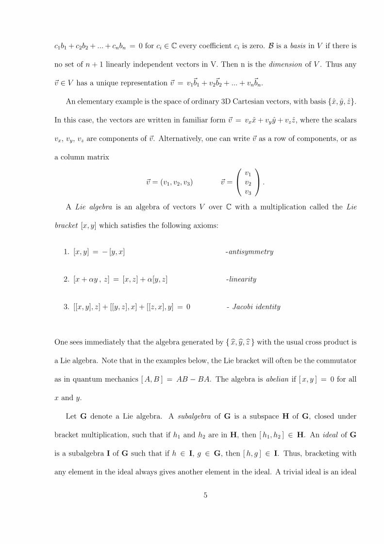
c1b1 + c2b2 + ... + cnbn = 0 for ci ∈ C every coefficient ci is zero. B is a basis in V if there is

no set of n + 1 linearly independent vectors in V. Then n is the dimension of V . Thus any

~v ∈ V has a unique representation ~v = v1~b1 + v2

~b2 + ... + vn~bn.

An elementary example is the space of ordinary 3D Cartesian vectors, with basis x, y, z.

In this case, the vectors are written in familiar form ~v = vxx + vyy + vz z, where the scalars

vx, vy, vz are components of ~v. Alternatively, one can write ~v as a row of components, or as

a column matrix

~v = (v1, v2, v3) ~v =

v1

v2

v3

.

A Lie algebra is an algebra of vectors V over C with a multiplication called the Lie

bracket [x, y] which satisfies the following axioms:

1. [x, y] = − [y, x] -antisymmetry

2. [x + αy , z] = [x, z] + α[y, z] -linearity

3. [[x, y], z] + [[y, z], x] + [[z, x], y] = 0 - Jacobi identity

One sees immediately that the algebra generated by x, y, z with the usual cross product is

a Lie algebra. Note that in the examples below, the Lie bracket will often be the commutator

as in quantum mechanics [ A,B ] = AB − BA. The algebra is abelian if [ x, y ] = 0 for all

x and y.

Let G denote a Lie algebra. A subalgebra of G is a subspace H of G, closed under

bracket multiplication, such that if h1 and h2 are in H, then [ h1, h2 ] ∈ H. An ideal of G

is a subalgebra I of G such that if h ∈ I, g ∈ G, then [ h, g ] ∈ I. Thus, bracketing with

any element in the ideal always gives another element in the ideal. A trivial ideal is an ideal

5

consisting of the entire algebra G or the ideal containing only the zero element. A simple

Lie algebra is one with no non-trivial ideals, and a semi-simple Lie algebra has no abelian

ideals.

As an example of an algebra that contains an abelian ideal, consider A generated by

translations and rotations in the xy plane. Thus, A = A, B, C where A = ∂∂x

, B = ∂∂y

,

and C = x ∂∂y− y ∂

∂x. One finds that

[A, C] = B , [B, C] = −A, [A, B] = 0 .

Thus, A and B form an abelian ideal in the algebra A.

A subalgebra K of G is called a Cartan subalgebra if K is nilpotent and of maximal

dimension[11], meaning that there is no other nilpotent subalgebra with greater dimension.

Thus for elements g1, g2 in a Cartan subalgebra K, [g1, g2] = 0, or in this subalgebra

all vectors commute. In physics, the dimension of the Cartan subalgebra corresponds to

the maximal number of quantum numbers of the system. One recalls that when a set of

Hermitian matrices commute, they can share a basis of mutual eigenvectors.

2.2 Structure of Lie Algebras

In order to understand further the structure of Lie algebras, it is useful to introduce the

adjoint representation of G. Each element x ∈ G can be thought of as a linear operator adx

acting on G, defined as

[ x, y ] = adx(y)

for all y ∈ G. Given a particular basis, the operators adx can be represented as matrices of

the General Linear group, GL(n,C), consisting of all complex non-singular n× n matrices.

6

The eigenspace formed by the adjoint operator adx with eigenvalue λ ∈ C is

y ∈ G|(adx− λ1)y = 0 .

Consequently, the generalized eigenspace of adx with eigenvalue λ is defined as

y ∈ G|(adx− λ1)ny = 0 for some n > 1 .

Since the generators K i of the Cartan subalgebra K have zero brackets amongst them-

selves, the matrices adk for all elements k ∈ K commute and hence are simultaneously

diagonalizable. Thus G is spanned by such elements y that are simultaneous eigenvectors of

all the maps adk, which satisfy

[ k, y ] = adk(y) = αy(k)y .

The purpose of the latter equation is to define αy(k). For any fixed element y ∈ G of this

type, the eigenvalue αy(k) of y is some complex number which depends linearly on k ∈ K.

In quantum theory, αy(k) is the quantum of excitation in an observable quantity k generated

by ladder operator y. Thus αy is a linear functional of k, because it maps K → C. (This is

a linear functional since it is linear and takes an element of the vector space into a complex

number.) The set of all eigenvalues (linear functionals) αyi forms a vector space K∗ dual

to K. The eigenvalues, αy(k), are the roots of the characteristic equation for k, thus αy is a

root of the algebra G.

G is spanned by elements satisfying (for y ∈ G)

[ k, y ] = αy(k)y .

Thus, G can be written as a direct sum of the Cartan subalgebra and the remaining 1-

dimensional vector spaces

G = K⊕⊕

α

C uα , (2.1)

7

which is called the Cartan decomposition of G relative to K [12]. Therefore, a semi-simple

Lie algebra is the direct sum of simple Lie algebras including the cartan subalgebra [2]

G = K⊕Gα1 ⊕Gα2 · · · ⊕Gα n .

This decomposition means that there exists a basis B of G which, apart from a basis of

the Cartan subalgebra, consists entirely of elements uαi∈ K⊥

α which satisfy

[ ki, uαi] = αyi

uαi.

The elements uαithat generate K⊥

α are the ladder operators associated to the roots α. Thus,

these eigenvectors are called root vectors.

The set of all roots of the algebra, which spans the dual space K∗, is denoted as Φ(G) and

called the root system of G. For semisimple Lie algebras, the root system is non-degenerate.

Thus, the eigenvectors are unique up to an overall constant. Therefore, the dimension of G

is equal to the dimension of K plus the number of roots. Also if α ∈ Φ(G), then −α ∈ Φ(G)

which I prove in the next section.

The basis of G is of the form

B = ki |i = 1, ..., r ∪ uαi|α ∈ Φ .

A basis of this form is called the Cartan-Weyl (canonical) basis of G [13]. From a physi-

cal point of view, the Cartan subalgebra ki|i = 1, ..., r is a complete set of commuting

observables, and the root vectors uαi|α ∈ Φ form a complete set of ladder operators.

Finite-dimensional Lie algebras have only finitely many roots, thus it is possible to divide

the roots into positive and negative roots, which correspond to, in quantum mechanics,

raising and lowering operators. Thus, Φ can be divided as follows

Φ+ = α ∈ Φ |α > 0 Φ− = α ∈ Φ |α < 0 .

8

This allows one to decompose further the algebra G

G = K⊥+ ⊕K⊕K⊥

−

This is called the Gauss decomposition of G [13].

2.2.1 The Killing Form

In order to understand better the relation between the roots, a geometrical picture of the

algebra is established through the Killing form. The Killing form is a pairing between

elements in the finite-dimensional Lie algebra (not a scalar product) G defined as

〈〈x, y 〉〉 = trace(adx ady) .

Thus, the Killing form is the trace of any matrix representing adx ady, independent of basis

(since the trace is independent of the choice of basis). Also, trace(AB)= trace(B A) for any

two square matrices A and B, so the Killing form is a symmetric bilinear form

〈〈x, y 〉〉 = 〈〈 y, x 〉〉 .

The Killing form is also an invariant form

〈〈 [x, y], z 〉〉 = 〈〈x, [y, z] 〉〉

According to Cartan’s Criterion for semi-simplicity [14], if and only if G is semi-simple, the

Killing form is non-degenerate. Thus,

〈〈x, y 〉〉 = 0 ∀ y ∈ G implies x = 0 .

From non-degeneracy of the Killing form, it can be shown that if α and β are any two roots

and β 6= −α, then from Eq.(2.1) the subalgebras Gα and Gβ are orthogonal relative to the

Killing form [14]. This fact allows one to prove that in any semi-simple Lie algebra, if α is a

9

root, then so is −α. In other words, for every raising operator, there must be a corresponding

lowering operator.

Proof. If z ∈ K and z ⊥ K (〈〈 z, k 〉〉 = 0), then z ⊥ G since by the above assertion that

Gα ⊥ Gβ for any two roots α and β, z ⊥ Gα ∀α 6= 0. Then, z = 0 by the non-degeneracy of

〈〈x, y 〉〉. If α is a root and −α is not a root, then Gα ⊥ Gβ for all roots β, so Gα ⊥ G. This

is a contradiction to the non-degeneracy of the Killing form, since 〈〈uα, ` 〉〉 = 0 ∀ ` ∈ G.

Also, one can show that the bracket product between a raising and lowering operator is

proportional to an element of the Cartan subalgebra with respect to this operation

〈〈 [ u−α, uα ], k 〉〉 = 〈〈u−α, uα 〉〉 kα .

Proof. 〈〈 [ u−α, uα ], k 〉〉 = 〈〈u−α, [ uα, k ] 〉〉 = 〈〈u−α, α(k) uα 〉〉 = α(k) 〈〈u−α, uα 〉〉 Now, take

the quantity [ u−α, uα ] = 〈〈u−α, uα 〉〉 kα and show it gives the same result. 〈〈 〈〈u−α, uα 〉〉 kα, h 〉〉 =

〈〈u−α, uα 〉〉 〈〈 kα, h 〉〉 = 〈〈u−α, uα 〉〉α(k) thus, [ u−α, uα ] = 〈〈u−α, uα 〉〉 kα.

This leads to a relation between different basis elements uα and uβ. Let k ∈ K, then

using Jacobi non-associativity,

[ k, [ uα, uβ ]] = [[ uβ, k ], uα ] + [ [ k, uα ], uβ ]

= [ uα, [ k, uβ ] ] + [ [k, uα ], uβ

= β(k)[ uα, uβ ] + α(k) [ uα, uβ ]

= (α + β)(k) [ uα, uβ ].

Thus, if α+β is not in Φ, then [ uα, uβ ] = 0 and if α+β is in Φ, then [ uα, uβ , uα] = nuα+β

for some integer n. A root α is called simple if α > 0 and it cannot be written as a sum of

two other positive roots. In general, the root system Φ is not linearly independent since the

10

Cartan subalgebra contains all linear combinations of its elements [αk1 + βk2] = (α + β)uα.

Thus, it is natural to seek a subset of Φ composed entirely of simple roots α, so that any

root β can be expressed as a linear combination of the simple roots.

To illustrate the connection between Lie algebras and physics, two simple examples are

presented in the next section.

2.3 Familiar Physical Examples

A clear example of applying Lie algebra to physics is the one-dimensional quantum Harmonic

oscillator problem. The Hamiltonian for the problem is

H = 12mω2

o x2 + 12m

p2 . (2.2)

The objective is to solve the eigenvalue equation

H|Ψ〉 = E|Ψ〉

for the energy eigenvalue E, and particular eigenfunction |Ψ〉 given the potential V (x) =

12mω2

ox2. The algebra is generated by the operators that correspond to physical quantities

in the problem, in this case the set H, p, x, 1, forms a basis. The constant 1 is included

because [ x, p ] is a constant. The Cartan subalgebra is composed of all operator combinations

that leave the number of energy quanta constant, hence do not change the overall energy of a

given state. It is clear that in this example, H and 1 form a basis for the Cartan subalgebra

[ H, H ] = 0 and [ 1, anything ] = 0, while [ H, x ], [ H, p ] 6= 0. To focus attention on the

essence of using Lie algebra, scale to dimensionless variables, such that m = k = ~ = 1,

H = 12p2 + 1

2x2 .

Now I review the idea of constructing ladder operators [15], but in the context of a Lie

11

algebra. In particular, how does one find raising and lowering operators? Thus consider the

following.

The subspace K⊥ complimentary to K is treated in the following way. First, form linear

combinations of the basis vectors spanning K⊥, so in the current example let B = αx + βp,

where α and β are numbers to be determined. The task is to calculate the coefficients α and

β such that B satisfies an operator eigenvalue equation of the form

[ H, B ] = λB ,

where operator B is a sort of eigenvector, and λ is its eigenvalue relative to H. After

calculating the left side, one gets

iβx− iαp = λ( αx + βp) .

Now recall that x and p are independent basis vectors in the Lie algebra. Thus, comparing

the coefficients of x and p,

iβ = λα and − iα = λβ .

Eliminating β, I reduce the two equations to the single equation

( 1− λ2 )α = 0 ,

so, either α = 0 or λ = ±1. The coefficient α cannot be zero, otherwise both α = 0 and

β = 0, so one gets the the following possible solutions:

either λ = +1 , β = −iα , B = α( x− ip ) ,

or λ = −1 , β = iα , B = α( x + ip) .

12

Therefore, we can rename the two possible solutions of B so as to correspond to the more

familiar a and a† notation. In order to normalize a and a† so that [ a, a† ] = 1, let α = 1√2.

One can easily see that B = 1√2( x + ip ), which prompts us to define a = B. Since both x

and p are Hermitian, a† = 1√2( x− ip ), which is the Hermitian conjugate of a. Continuing,

as usual [15]

aa† =(

1√2

)2

( x− ip )( x + ip )

= 12( x2 + p2 + i[x, p] ) .

Thus,

a†a = H − 12

and aa† = H + 12

,

which allows two equivalent expressions for the Hamiltonian H = a†a+ 12

and H = aa†− 12.

Now, one can solve the time-independent Schrodinger equation H|Ψ〉 = E|Ψ〉 easily ( as

Schodinger did [16] ) by using the operator a in the eigenvalue equation

[ H, a ] = −a .

So, operating on an arbitrary eigenfunction |Ψ〉, with eigenvalue E, one gets

[ H, a ]|Ψ〉 = −a|Ψ〉 ,

and then, because in quantum mechanics the Lie product is the commutator,

H( a|Ψ〉 )− a( H|Ψ〉 ) = −( a|Ψ〉 )

H( a|Ψ〉 )− E( a|Ψ〉 ) = −( a|Ψ〉 ) ,

therefore

H( a|Ψ〉 ) = ( E − 1 )( a|Ψ〉 ) .

There are two possibilities:

13

1. a|Ψ〉 is a new eigenfunction with energy E − 1, or

2. a|Ψ〉 = 0, corresponding to a ground state.

One can continue the harmonic oscillator example to determine all of its physical properties.

It is presented here rather as a simple template for the general idea of constructing ladder

operators in the language of Lie algebras as described generally below.

Another familiar example is that of angular momentum. Consider the generalized angular

momentum operators Jx, Jy, and Jz, which satisfy the commutation rules

[ Jx, Jy ] = iJz , [ Jy, Jz ] = iJx , [ Jz, Jx ] = iJy .

From these operators, one can construct the Casimir operator J2 = ~J · ~J , which commutes

with all of the angular momentum operators

[ J2, Jx ] = [ J2, Jy ] = [ J2, Jz ] = 0 .

Thus, the angular momentum algebra J is generated by Jx, Jy, Jz, J2 . J is an extension

in SU(2) of the algebra generated by Jx, Jy, Jz . It is important to note that the casimir

operator J2 only has meaning for representations, and not as an element of the algebra since

products like J2x do not exist in J.

Next, choose a basis for the Cartan subalgebra K of elements that mutually commute.

By convention we usually choose J2, Jz . Again, form a vector A = αJx + βJy, which is

a linear combination of elements outside the Cartan sububalgebra. The rest of the algebra

K⊥ should be spanned by vectors that are mutual eigenvectors of the Cartan subalgebra so,

[ J2, A ] = 0 ,

[ Jz, A ] = λA .

14

Notice that the fact that the operators in K commute guarantees they have mutual eigen-

vectors. We continue by using the linearity property of the bracket

[ Jz, A ] = [ Jz, (αJx + βJy) ] = α[ Jz, Jx ] + β[ Jz, Jy ] .

Thus, from this and the commutation rules of the angular momentum operators, one gets

the following relation:

αiJy − βiJx = λ( αJx + βJy ) .

Comparing the coefficients, gives

α = −iλβ , β = iλα .

These equations are homogeneous, so I am free to choose α = 1. Thus,

either λ = +1 , β = +i ,

or λ = −1 , β = −i .

Substituting the α and β solutions into the expression for the vector A, I get

A = J1 ± iJ2

As in the harmonic oscillator example, this is how we arrive at the familiar ladder operators

used in elementary quantum mechanics

J± = Jx ± iJy . (2.3)

If one chooses as a basis of J the set J+, J−, Jz, the elements can be represented in adjoint

form:

adJz =

i 0 00 −i 00 0 0

, adJ+ =

0 0 10 0 00 2 0

, adJ− =

0 0 00 0 1−2 0 0

. (2.4)

15

Notice that with this choice of basis, the matrix corresponding to the element in the Cartan

subalgebra K is diagonal. In general, this is part of the reason why ladder operators are

constructed. The raising and lowering operators along with the operators within the Cartan

subalgebra provide a convenient basis for the entire algebra G. Therefore, the basis that

spans K⊥ is always arranged so that adk for all k ∈ K is diagonal, this is the Cartan-Weyl

basis B.

And so, in this section two examples from elementary quantum mechanics have been

presented to illustrate the process of finding appropriate ladder operators. In the following,

this method of constructing root vectors will be applied to the Lie algebras of an anisotropic

oscillator in a magnetic field (including electron spin via perturbation theory) and of a

solvable 3-body problem.

16

CHAPTER 3

CONFINED PARTICLE IN A MAGNETIC FIELD

Begin by setting up the Hamiltonian for a charged particle in a magnetic field. For

simplicity, consider a constant magnetic field in the positive z direction. Thus, the magnetic

field is ~B = Bo z, which suggests a possible gauge potential

~A(~r) = 12

Bo (x y − y x) . (3.1)

Also, ignoring spin, the Hamiltonian for a charged particle in a magnetic field is, in general

H =1

2m

(~p− q

c~A)·(~p− q

c~A)

+ V (~r) .

In this case, we add a containment force, an anisotropic harmonic restoring force, so that

calculation may apply in some abstract way to a quantum dot. This force suggests the

following choice of potential:

V (~r) = 12mα2 ( x2 + y2 ) + 1

2mβ2z2 . (3.2)

Therefore, the Hamiltonian for a charged particle in a constant magnetic field, under the

influence of the containment force is

H = 12m

∣∣∣~p− q

c~A∣∣∣2

+ 12mα2 ( x2 + y2 ) + 1

2mβ2z2 . (3.3)

Expanding the terms of the Hamiltonian one gets

~A · ~p = 12Bo (x py − y px) = 1

2Bo Lz, A2 = 1

4B2

o (x2 + y2).

17

After simplifying, it is clear that the Hamiltonian decouples into separate terms, one for the

xy plane and another for the z direction

H = Hxy + Hz .

The z terms in the Hamiltonian make up a one-dimensional oscillator

Hz = 12 m

p2z + 1

2mβ z2,

and the other term constitutes a Hamiltonian for the xy motion,

Hx,y = 12m

(p2x + p2

y) − 12 m

qcBo Lz + 1

2 mq2

c214B2

o (x2 + y2) + 12mα2 (x2 + y2)

=1

2m(p2

x + p2y) −

(q Bo

2 mc

)Lz +

1

2m

(α2 +

q2 B2o

4 m2 c2

)(x2 + y2) .

This motivates the definitions

ωb =q Bo

2 mc, and Ω =

√α2 + ω2

b ,

where ωb is the Larmor frequency. Thus, the xy part of the Hamilton simplifies to

Hxy = 12m

(p2x + p2

y) − ωb Lz + 12m Ω2 (x2 + y2). (3.4)

We now focus specifically on Hxy, since the solution to the z-degree of freedom corresponding

to a one-dimensional harmonic oscillator is straight-forward. Again, the objective is to

solve the eigenvalue equation H|Ψ〉 = E|Ψ〉 for all allowed energies. In this problem,

Hxy, Lz, px, py, x, y, 1 forms a basis of the algebra A. As usual, one can construct

orbital angular momentum out of these basis elements. In this problem, we only consider the

z component of the total angular momentum Lz = xpy− ypx, since it will be conserved due

to the oblate spheroidal symmetry of the potential. It is clear that the Cartan subalgebra K

for this problem is spanned by Hxy, Lz, 1 , since Hxy and Lz commute. Before proceeding

18

further, we compute the Lie bracket product for elements of K with the basis elements.

Starting with Lz, I have

[Lz, x] = [−y px, x] = i ~ y, [Lz, y] = −i ~x,

[Lz, px], = [x py, px] = i ~ py, [Lz, py] = − i ~ px .

One can see that commutators of the form

[Lz, f(x2 + y2)], and [Lz, g(p2x + p2

y)]

vanish, for any functions f and g, and hence [ Lz, Hx,y ] = 0, so Lz is indeed conserved

(corresponding to a good quantum number). For completeness, I continue computing bracket

products of H with each of the other basis vectors of the algebra:

[ Hxy, x ] = − i ~m

px − i ~ωb y

[ Hxy, y ] = − i ~m

py + i ~ωb x

[ Hxy, px ] = − i ~ωb py + i ~m Ω2 x

[ Hxy, py ] = + i ~ωb px + i ~m Ω2 y

(3.5)

Once the general form of the bracket product [ k, y ] (k ∈ K, y ∈ A) is determined, one can

construct an orthonormal basis for the algebra more easily. In order to form the eigenvector,

or root vector u (a quantum mechanical operator), which is a linear combination of all the

basis elements not in K, one introduces undetermined coefficients

u = a1 x + a2 y + b1 px + b2 py .

We wish to choose these coefficients (a1, a2, b1, b2) such that u satisfies simultaneously the

eigenvalue equations

[Lz, u] = λu ,

19

[Hxy, u] = ε u .

These are in fact matrix eigenvalue equations for adLz and adHxy which operate on the

algebra. It is customary to describe them simply as eigenvalue equations where operator u

(ladder operator) is the eigenvector and λ and ε are the respective eigenvalues. Starting with

the Lz eigenvalue equation, one finds

[Lz, u] = a1 [Lz, x] + a2 [Lz, y] + b1 [Lz, px] + b2 [Lz, py]

= i ~ a1 y − i ~ a2 x + i ~ b1 py − i ~ b2 px.

= λu (3.6)

After comparing the coefficients from each side of Eq.(3.6) we have

λ a1 = − i ~ a2, λ a2 = i ~ a1, λ b1 = − i ~ b2, λ b2 = i ~ b1.

There are two possibilities, either λ = +~ or λ = −~.

λ = +~ ⇒ a2 = i a1, b2 = i b1 ,

λ = −~ ⇒ a2 = − i a1, b2 = − i b1.

For the second eigenvalue equation involving Hxy, we get

[Hxy, u] = a1 [Hxy, x] + a2 [Hxy, y] + b1 [Hxy, px] + b2 [Hxy, py]

= a1 (− i ~m

px − i ~ωb y) + a2 (− i ~m

py + i ~ωb x)

+b1 (− i ~ωb py + i ~m Ω2 x) + b2 (+ i ~ωb px + i ~m Ω2 y) .

Comparing the coefficients as in the case for Lz,

ε a1 = + i ~ωb a2 + i ~m Ω2 b1,

20

ε a2 = − i ~ωb a1 + i ~m Ω2 b2,

ε b1 = − i ~m

a1 + i ~ωb b2,

ε b2 = − i ~m

a2 − i ~ωb b1 .

Now, of course there are two choices for the relation between a1 and a2 also between b1 and

b2, which correspond to the choice of λ = ±~. When λ = +~, a2 = i a1 and b2 = i b1 so

ε a1 = − ~ωb a1 + i ~m Ω2 b1,

i ε a1 = − i ~ωb a1 − ~m Ω2 b1,

ε b1 = − i ~m

a1 − ~ωb b1,

i ε b1 = +~m

a1 − i ~ωb b1,

So

(ε + ~ωb) a1 = i ~m Ω2 b1,

(ε + ~ωb) b1, = − i ~m

a1 .

Eliminating b1, I reduce two equations to one

(ε + ~ωb)2 a1 = ~2 Ω2 a1, or ε = ~ (±Ω− ωb) .

Similarly, when λ = −~, one has a2 = −i a1 and b2 = −i b1, so

ε a1 = + ~ωb a1 + i ~m Ω2 b1,

− i ε a1 = − i ~ωb a1 + ~m Ω2 b1,

ε b1 = − i ~m

a1 + ~ωb b1,

− i ε b1 = − ~m

a1 − i ~ωb b1 .

21

Again, the four equations reduce to the following two:

(ε − ~ωb) a1 = i ~m Ω2 b1,

(ε − ~ωb) b1, = − i ~m

a1 .

Finally, for the choice of λ = −~, one has

(ε − ~ωb)2 a1 = ~2 Ω2 a1, or ε = ~ (±Ω + ωb) .

Thus we have four operators in the following table.

Table 1: Complete Set of Ladder Operators

λ ε operator

1. + ~ ~ (−Ω− ωb) u = 12

√m Ω~

(x + i y + i

m Ωpx − 1

m Ωpy

)

2. − ~ ~ (+Ω + ωb) u† = 12

√m Ω~

(x− i y − i

m Ωpx − 1

m Ωpy

)

3. − ~ ~ (−Ω + ωb) v = 12

√m Ω~

(x− i y + i

m Ωpx + 1

m Ωpy

)

4. + ~ ~ (+Ω− ωb) v† = 12

√m Ω~

(x + i y − i

m Ωpx + 1

m Ωpy

)

To make the operators dimensionless, notice that the quantity

b =

√~

m Ω

has units of length. The operators in the table have been chosen with the following normal-

ization:

[u, u†] = 1, [v, v†] = 1,

[u, v] = 0, [u, v†] = 0 . (3.7)

Since the eigenvalues ε and λ are computed using the results of adLz(y) and adHxy(y)

for all y in A, they constitute the roots of the algebra. Notice that the roots are non-

degenerate and appear in ± pairs, which is a consequence of semi-simplicity (section 2.2.1).

22

Once the operators are constructed, one considers the eigenvalue equations corresponding

to the members of K, the Cartan subalgebra. These eigenvalue equations permit explicit

calculation of the ground state, since successive application of the the lowering operators must

eventually annihilate the state function |ψ`,k〉. I denote the energy and angular momentum

quantum numbers as k and ` respectively. Starting with the angular momentum operator,

[Lz, u]|ψ`,k〉 = ~u|ψ`,k〉

Lz u|ψ`,k〉 − uLz|ψ`,k〉 = ~u|ψ`,k〉

Lz(u|ψ`,k〉) = (` + 1) ~ |ψ′`,k〉 .

Thus, either u|ψ`,k〉 = 0 or ψ′`,k is a new eigenvector with eigenvalue (not normalized) (`+1)~

for Lz. Similarly,

[Hxy, u] |ψ`,k〉 = ~ (−ωb ± Ω)u|ψ`,k〉

Hxy u|ψ`,k〉 − uHxy|ψ`,k〉 = ~ (−ωb ± Ω) u|ψ`,k〉

Hxy(u|ψ`,k〉) =(k − ~(Ω + ωb)

)|ψ′`,k〉

Again, either |ψ′`,k〉 = 0 or else k − ~(Ω + ωb) is an eigenvalue for Hxy. Therefore, either

|ψ′`,k〉 = 0 or |ψ′`,k〉 = (const.)|k − ~(Ω + ωb), ` + 1〉. Since the squared norm of a vector

cannot be negative, it must be that

〈ψ`,k | u† u | ψ`,k〉 =‖ u | ψ`,k〉 ‖2 ≥ 0 .

The next step is to solve for what ` and k must be. The product of u† and u is

u† u =1

2~Ω(Hxy + ωbLz)− Lz

2~− 1

2

so

(C1)2 = 〈ψ`,k|u† u|ψ`,k〉 =

k

2Ω~+

`

2(ωb

Ω− 1)− 1

2(3.8)

23

In a similar manner, either v|ψ`,k〉 = 0 or v|ψ`,k〉 = C2|ψ′′`,k〉, where the product of v† and

v is

v†v =1

2~Ω( Hxy + ωbLz ) +

Lz

2~− 1

2

Thus, the inner product is

(C2)2 = 〈ψ`,k|v† v|ψ`,k〉 =

k

2Ω~+

`

2(ωb

Ω+ 1)− 1

2(3.9)

Starting from any mutual eigenstate of Hxy and Lz and operating successively with u, each

time lowering the squared norm, one must eventually get to a state |ψ〉 such that u|ψ〉 = 0.

However, since [ u, v ] = 0, and [ u, v† ] = 0, it follows that u also annihilates v|ψ〉 and

v†|ψ〉 or any power (v†)p|ψ〉. Thus, u annihilates an infinite set of |ψ〉. Starting with |ψ〉

annihilated by u, and lowering successively with v one must arrive at a unique state |ψo〉

such that u|ψo〉 = 0 and v|ψo〉 = 0. Setting the right hand sides of Eqs. (3.8) and (3.9)

equal to zero, I get for the ground state

` = 0 and k = ~Ω

So one is looking for the ground state |ψ`,k〉 which is the unique, normalized solution of

u|ψo〉 = 0 and v|ψo〉 = 0 .

Transferring the u operator in particular from Dirac to coordinate representation, one has

the following differential equation

uψo(x, y) =1

2

√mΩ

~

(x + iy +

~mΩ

∂

∂x+

i~mΩ

∂

∂y

)ψo(x, y) = 0 . (3.10)

A linear partial differential equation of this form can be solved by standard means. The

solution is of exponential form ψo(x, y) = eφ. Substitution of this trial solution into the

24

differential equation Eq.(3.10) and invoking the definition of b, yields the following result

∂φ

∂x+ i

∂φ

∂y=−1

b 2(x + iy) . (3.11)

In order to solve this partial differential equation, invoke the method of characteristics [17].

The basic strategy is to convert the coordinates (x, y) to a new system of coordinates in which

the partial differential equation becomes a pair of ordinary differential equations. These

new coordinates are the characteristic variables or canonical coordinates of the differential

equation. Thus, Eq.(3.11) is converted into two ordinary differential equations

dx

1=

dy

i=

−b 2

(x + iy)dφ . (3.12)

Solving the first ODE, one obtains the characteristic ξ = x + iy. Using this coordinate

(considered constant) in the second ODE from Eq.(3.12) and solving for φ, one finds that

φ = − ξb 2 x + f(ξ). So, one has determined φ up to a constant function f(ξ). The partial

differential equation vψo = 0 must also be satisfied, which by the same method outlied for

uψo = 0 leads to the second canonical coordinate for this system η = x− iy.

Therefore, by the first PDE (uψo = 0) the ground state is of the form

ψo = f(x + iy) e−x(x+iy)

b2 .

In order to know what the function f actually is, recall that ψo must be annihilated by v.

Thus, applying v to the current result gives the first-order ordinary differential equation

bf ′(x + iy)− (x + iy)f(x + iy) = 0 (3.13)

solving this, and normalizing the result gives the true ground state

ψo(x, y) =1

b√

πe(−mΩ

2~ (x2+y2)). (3.14)

25

We can see from their commutation with the Cartan subalgebra, Table 1, that the raising

operators u† and v† have the following effect on the energy and angular momentum quantum

numbers of the wave function:

u† : ` → `− 1, k → k + ~(Ω + ωb)

v† : ` → ` + 1, k → k + ~(Ω− ωb) .

Every state can be constructed from the ground state by raising n1 times with u†, and raising

n2 times with v†. We can reorganize the quantum numbers according to the number of times

u† and v† would have to operate. Thus the angular momentum quantum number ` is

` = n2 − n1

and the energy eigenvalue is

E = (n1 − n2)~ωb + (n1 + n2 + 1)~Ω

= kω~ωb + kΩ~Ω .

Using these rules, I reorganize the quantum numbers and define a new basis |n1, n2〉 for

Hxy. The next task is to calculate the normalization constant C1 such that u†|n1, n2〉 =

C1|n1 + 1, n2〉. This facilitates calculating all subsequent states.

u†|n1, n2〉 = C1|n1 + 1, n2〉

〈n1, n2|uu†|n1, n2〉

C12 =

1

2(1 + n1 + n2) +

ωb

2Ω(n1 − n2) +

ωb

2Ω(n2 − n1)− 1

2(n2 − n1) +

1

2

Simplification yields

C21 = n1 + 1 ,

26

hence

C1 =√

n1 + 1.

Also

v†|n1, n2〉 = C2|n1, n2 + 1〉 ,

C22 =

1

2(1 + n1 + n2) +

ωb

2Ω(n1 − n2) +

ωb

2Ω(n2 − n1) +

1

2(n2 − n1) +

1

2,

C22 = n2 + 1 .

Therefore, as expected

C2 =√

n2 + 1.

Now one gets all the allowed states by application of the operators u† and v†, which raise the

quantum numbers n1 and n2 associated with the xy-degrees of freedom of the Hamiltonian,

and of a†z, which raises the z quantum number n3. These operators can be applied n1, n2,

and n3 times respectively. The general formula for the normalized state |n1, n2, n3〉 is

(az†)n3 (v†)n2 (u†)n1|0, 0, 0〉 =

√n1!

√n2!

√n3! |n1, n2, n3〉 . (3.15)

3.1 A Generating Function

Let us restrict attention to Hxy. A more convenient method to manipulate all excited states

at once is to use a generating function. To obtain the excited state ψn1,n2(x, y) recall first

that

u† v† ψn1,n2(x, y) =√

n1 + 1√

n2 + 1 ψn1+1,n2+1(x, y) ,

and thus the n1, n2 excited state is

ψn1,n2(x, y) =1√n1!

1√n2!

(u†)n1(v†)n2ψo(x, y) . (3.16)

27

To illustrate the general method, consider first the form of a generating function for a set

of single variable functions of x. The familiar definition [18] of a generating function for an

infinite set of functions fn(x) is

G(x, t) =∞∑

n = 0

Cn fn(x) tn (3.17)

where the constant Cn depends in some preassigned way on n, but is independent of x and

t. For the current problem, one is looking to obtain a generating function for the set of

eigenfunctions ψn1,n2(x, y), which depends on both x and y. Therefore, in view of the way

v† and u† act, a convenient generating function would appear to be of the following form:

F (x, y, s, t) =∑n1,n2

Cn1Cn2sn1tn2ψn1,n2(x, y)

=∑n1,n2

1√n1!

1√n2!

sn1tn2ψn1,n2(x, y) .

Using Eq.(3.16), one can recover an exponential expansion,

F (x, y, s, t) =∑n1,n2

1

n1!n2!sn1tn2(u†)n1(v†)n2ψo(x, y)

= exp(su† + tv†)ψo(x, y) . (3.18)

In the latter equation, I have used the fact that [u†, v†] = 0. The reader may recognize this

as a coherent state, an eigenstate of the lowering operator of the Hamiltonian, (the coherent

state of the 1-D harmonic oscillator can be written as |α〉 = e−α2

2

∑∞n=0

αn√n!|n〉) [19]. The

group-theoretic method employed in the following to obtain a generating function is the

Weisner method [20]. This method relies on the fact that certain partial differential equations

are invariant with respect to a nontrivial continuous group of transformations (a Lie group).

The strategy is to find canonical variables such that u† and v† are essentially derivatives and

then to evaluate Eq.(3.18) via the Taylor theorem. The canonical coordinates for the two

28

PDE’s uψ0 = 0 and vψ0 = 0, are ξ = x + iy and η = x− iy, so to make these coordinates

dimensionless we introduce the new coordinates ζ and ζ∗.

ζ =x + iy

b√

2

ζ∗ =x− iy

b√

2.

Solving for x and y

x =b√2(ζ + ζ∗)

y =−ib√

2(ζ − ζ∗)

Hence, from the chain rule

∂

∂ζ=

∂x

∂ζ

∂

∂x+

∂y

∂ζ

∂

∂y

∂

∂ζ∗=

∂x

∂ζ∗∂

∂x+

∂y

∂ζ∗∂

∂y.

After taking the appropriate derivatives, one obtains the following expressions:

∂

∂ζ=

b√2

(∂

∂x− i

∂

∂y

)

∂

∂ζ∗=

b√2

(∂

∂x+ i

∂

∂y

)

Inserting the definitions of px and py, I convert the two operators u† and v† into

u† =1√2

(x− iy

b√

2− b√

2

(∂

∂x− i

∂

∂y

))

v† =1√2

(x + iy

b√

2− b√

2

(∂

∂x+ i

∂

∂y

)),

thus using ζ and ζ∗

u† =1√2

(ζ∗ − ∂

∂ζ

),

v† =1√2

(ζ − ∂

∂ζ∗

).

29

The next goal is to relate u† and v† each by a gauge transformation to a derivative operator,

and then to evaluate the generating function by summing a Taylor series, thus treating

exp (α d/dx) as a shifting operator. The Taylor series expansion of F (x + α) can be written

in terms of a derivative operator on F (x), an example of a 1-parameter Lie group [21].

F (x + α) = F (x) + αF ′(x) +α2

2!F ′′(x) + · · ·

=

(1 + α

d

dx+

α2

2!

d2

dx2+ · · ·

)F (x) = e(α d

dx)F (x) .

(3.19)

Therefore, the operator exp(α d

dx

)translates the function F (x) by an amount α. Thus,

starting with u†, suppose one has a function µ = µ(ζ, ζ∗)

u† = − 1√2

1

µ

∂

∂ζµ ,

then by the Leibniz rule for differentiating a product

u† = − 1√2

(∂

∂ζ+

1

µ

∂µ

∂ζ

)

so, comparing to the expression above for u†

1

µ

∂µ

∂ζ= −ζ∗

this is a separable differential equation, so holding ζ∗ constant

ln µ = f(ζ∗)− ζζ∗ .

Solving for the integrating factor µ, it is not necessary to retain the arbitrary constant of

integration f(ζ∗) since only a particular solution is required, so

µ = e−ζζ∗ .

30

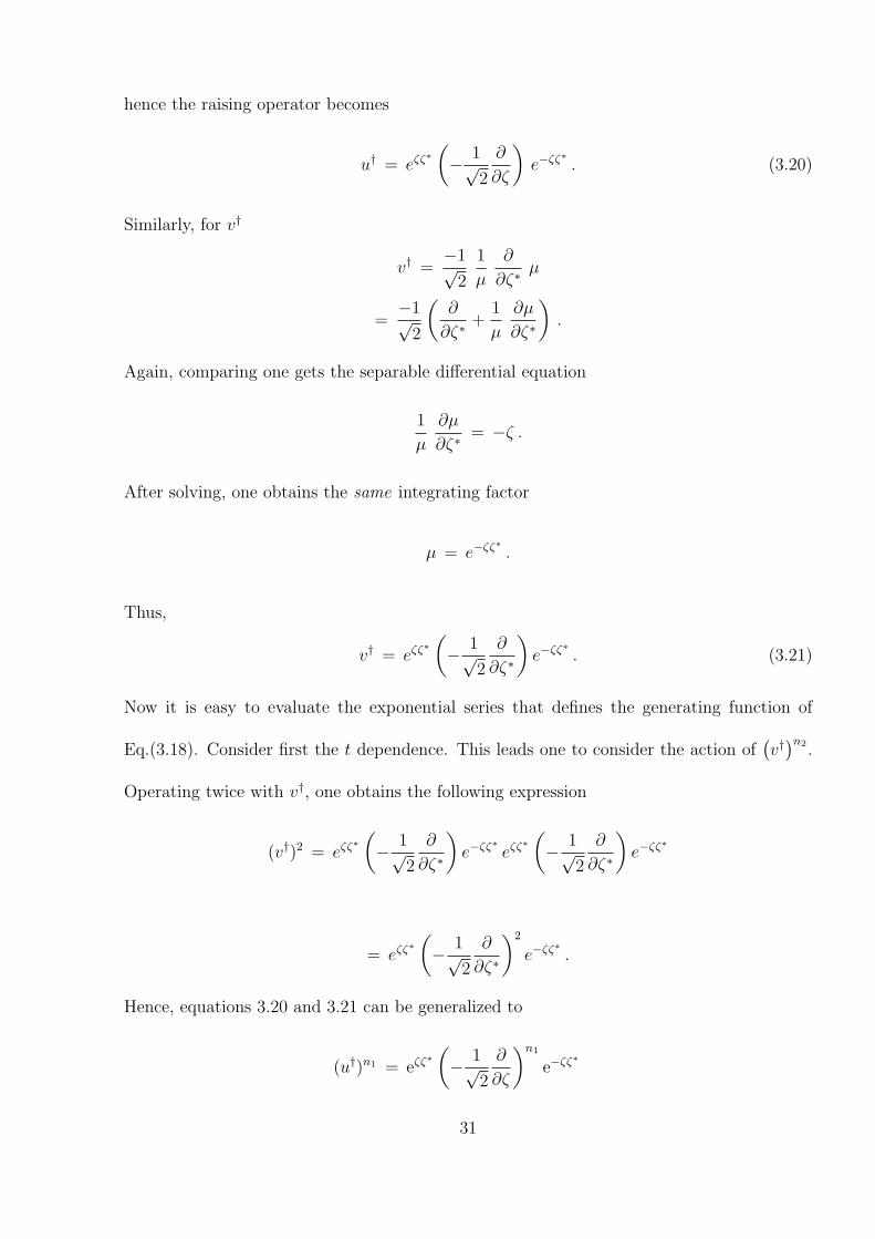
hence the raising operator becomes

u† = eζζ∗(− 1√

2

∂

∂ζ

)e−ζζ∗ . (3.20)

Similarly, for v†

v† =−1√

2

1

µ

∂

∂ζ∗µ

=−1√

2

(∂

∂ζ∗+

1

µ

∂µ

∂ζ∗

).

Again, comparing one gets the separable differential equation

1

µ

∂µ

∂ζ∗= −ζ .

After solving, one obtains the same integrating factor

µ = e−ζζ∗ .

Thus,

v† = eζζ∗(− 1√

2

∂

∂ζ∗

)e−ζζ∗ . (3.21)

Now it is easy to evaluate the exponential series that defines the generating function of

Eq.(3.18). Consider first the t dependence. This leads one to consider the action of(v†

)n2 .

Operating twice with v†, one obtains the following expression

(v†)2 = eζζ∗(− 1√

2

∂

∂ζ∗

)e−ζζ∗ eζζ∗

(− 1√

2

∂

∂ζ∗

)e−ζζ∗

= eζζ∗(− 1√

2

∂

∂ζ∗

)2

e−ζζ∗ .

Hence, equations 3.20 and 3.21 can be generalized to

(u†)n1 = eζζ∗(− 1√

2

∂

∂ζ

)n1

e−ζζ∗

31

(v†)n2 = eζζ∗(− 1√

2

∂

∂ζ∗

)n2

e−ζζ∗

(3.22)

This allows one to express F (x, y, s, t) as a function of ζ and ζ∗. Let f(ζ, ζ∗, s, t) =

f(x(ζ, ζ∗), y(ζ, ζ∗), s, t). Inserting the expressions for (u†)n1 and (v†)n2 from Eqs.(3.22), one

obtains

f(ζ, ζ∗, s, t) =∑n1,n2

1

n1!n2!sn1 eζζ∗

(− 1√

2

∂

∂ζ

)n1

e−ζζ∗

·tn2eζζ∗(− 1√

2

∂

∂ζ∗

)n2

e−ζζ∗ ψo(ζ, ζ∗)

=1

µ(ζ, ζ∗)

∑n1,n2

1

n1!n2!

(− s√

2

∂

∂ζ

)n1(− t√

2

∂

∂ζ∗

)n2

µ(ζ, ζ∗)ψo(ζ, ζ∗)

=1

µ(ζ, ζ∗)exp

(− s√

2

∂

∂ζ

)exp

(− t√

2

∂

∂ζ∗

)µ(ζ, ζ∗) ψo(ζ, ζ∗)

Therefore, by Eq.(3.19) the function f(ζ, ζ∗, s, t) is translated in ζ by an amount s√2

and in

ζ∗ by an amount t√2, which leads to the following closed-form expression for the generating

function:

f(s, t, ζ, ζ∗) =1

µ(ζ, ζ∗)µ

(ζ − s√

2, ζ∗ − t√

2

)ψo

(ζ − s√

2, ζ∗ − t√

2

).

Expressing the ground state in terms of ζ and ζ∗

ψo(ζ, ζ∗) =1

b√

πe−ζζ∗ , (3.23)

one finally obtains the generating function

f(s, t, ζ, ζ∗) = e−ζζ∗ e−(ζ−s/√

2)(ζ∗−t/√

2) 1

b√

πe−(ζ−s/

√2)(ζ∗−t/

√2)

32

=1

b√

πe−ζζ∗ exp

(2ζ

s√2

+ 2ζ∗t√2− st

)

= ψo(ζ, ζ∗) exp

(2ζ

s√2

+ 2ζ∗t√2− st

).

Transforming back to the original cartesian coordinates,

f(s, t, x, y) = ψo(x, y) exp

[(x + iy)s

b+

(x− iy)t

b

]e−st , (3.24)

a convenient generating function has been constructed that allows one to obtain all of the

possible excited states easily. Hence, expanding in powers of s and t and taking coefficients

(multiplying the nth coefficient by√

n! ), one can obtain the desired quantum states. For

example, the first four are as follows:

ψ0,0 =1

b√

πe−(x2+y2)

2b2

ψ0,1 =(x + iy)

b2√

πe−(x2+y2)

2b2

ψ1,0 =(x− iy)

b2√

πe−(x2+y2)

2b2

ψ1,1 =(x2 + y2 − b2)

b3√

πe−(x2+y2)

2b2

Before going further, simplify the calculations by writing x, y, px and py in terms of the

operators u, u†, v, v†. Using the definitions of the ladder operators one has

x =1

2b(u + u† + v + v†) ,

y =i

2b(u† − u + v − v†) ,

px =mΩ

2ib(u− u† + v − v†) ,

py =mΩ

2b(v + v† − u− u†) .

(3.25)

Implementing Eqns.(3.25), gives the general energy eigenvalue for the Hamiltonian Hxy in

more transparent form. Start by rewriting the Hamiltonian, Eq.(3.4), in terms of the oper-

33

ators u, u†, v, and v†. Thus, with the normalization expressed in Eq.(3.7)

Hxy = 12m

(p2x + p2

y) + 12m Ω2 (x2 + y2)− ωb Lz

= ~Ω4

(uu† + u†u + vv† + v†v − 2uv − 2u†v†

)

+~Ω4

(uu† + u†u + vv† + v†v + 2uv + 2u†v†

)

−~ωb

2

(vv† + v†v − uu† − u†u

).

After simplification, the xy portion of the Hamiltonian becomes

Hxy =~Ω4

(uu† + u†u + vv† + v†v) +ωb~2

(uu† + u†u− vv† − v†v) . (3.26)

In order to calculate the energy, I insert this into the Schrodinger equation H | Ψn〉 = E |

Ψn〉, where |ψn〉 = |n1, n2, n3〉 so

En1n2n3 = 〈n1, n2, n3|Hxy|n1, n2, n3〉 .

Thus, simple calculation gives

En1n2n3 =~Ω2

(n1 + n2 + 1)− ωb~(n2 − n1) + ~β(n3 +1

2) . (3.27)

A plot of this result as a functioin of the Larmor frequency is shown in Figure 1.

3.2 Selection Rules

If one wishes to allow for transitions from one energy level to another, a time-dependent

potential is introduced. The time-dependent portion of the Hamiltonian is assumed to be

small compared to the time-independent part, thus the time-dependent Hamiltonian Hrad is

treated as a perturbation (time-dependent perturbation theory). Thus the full Hamiltionian

of the problem becomes

H(t) = Ho + Hrad(t) .

34

Figure 1: Plot of Energy as a Function of the Larmor Frequency.

Fermi’s golden rule is an expression that gives the rate of transition from |ψi〉 to |ψf〉

Γ =2π

~|〈ψf |Hrad|ψi〉|2ρ(Ef )δ(Ef − Ei ± ~ω) , (3.28)

which is due to the absorption or emission of a photon. The ρ(Ef ) term in Eq.(3.28) denotes

the density of final states and the δ(Ef −Ei±~ω) allows only for transitioins between states

of equal energies.

Specifically, the time dependence comes from an electic field ~E(~r, t) which is not assumed

to be constant (∇φ = 0 at t = 0) thus,

~E(~r, t) =∂ ~A(~r, t)

∂t.

As usual, the time and position dependence of this vector potential are assumed to be

exponential. This is distinct from the vector potential ~Ab(~r) due to the static magnetic field

in the problem, thus it is denoted

~Arad(~r, t) = Ao ε ei(~k·~r−ωt) ,

which satisfies the Coulomb gauge condition ∇ · ~Arad = 0. Due to the linearity of the

electomagnetic field, ~A(~r, t) = ~Ab(~r)+ ~Arad(~r, t). Thus, the system is coupled to the radiation

35

through the time dependent Hamiltonian

Hrad(t) =q

c~Arad · ~p .

The time dependent portion of this Hamiltonian forms the energy-conserving delta functions.

Also, the incident photon has a given polarization ε and wave vector ~k = 2πλ

k which are

assumed to always be mutually perpendicular (the angular frequency is ωk = ck). Thus,

the time dependent Hamiltonian is

Hrad = Aoe±i~k·~r ε · ~p

= Ao

(1± i

2π

λk · ~r ± · · ·

)(ε · ~p) . (3.29)

In order to compute the selection rules, one need only consider matrix elements between the

initial and final states. Clearly a non-zero result indicates an allowed transition. In most

problems, the first term in the expansion Eq.(3.29) dominates, which is the electric dipole

term (ε · ~p). The extent to which the other terms of the expansion contribute depends on

a length ratio. The second term in the expansion, the magnetic dipole plus the electric

quadrupole, has a strength on the order of aλ, where a is the diameter of the problem of

interest. For an atomic or molecular problem, the diameter a is usually much smaller than

λ. However in this case a quantum dot is considered, which has a diameter much larger

than that of the typical atomic problem. Therefore, presumably the higher multipole terms

are more important. One can readily compute the matrix elements between final and initial

states by writing ~p and ~r in terms of the ladder operators of the problem. The lowest-order

electric dipole transitions were computed by considering

〈n1f n2f n3f |ε · ~p |nn1i n2i n3i〉 ,

while the lowest order magnetic dipole and electric quadrupole terms were calculated through

36

elements of the form

〈n1f n2f n3f |(ε · ~p)(k · ~r)|n1i n2i n3i〉 .

Selected results are displayed in Table 2.

3.3 A Charged Particle with Spin

The next step is to make the problem perhaps a bit more realistic by adding spin to the

particle. In order to form the spin Hamiltonian, I take into account spin-orbit coupling, as

well as Zeeman energy. Thus, assume the spin portion of the Hamiltonian is

Hspin = −~µ · ~B (3.30)

where the magnetic field in the electron’s frame of reference [22] is

~Belectron = ~Bo − ~v

c× ~Elab , (3.31)

where ~Bo is the applied field in the laboratory frame ( ~Bo = ~Blab),

~Elab = −∇φ

and

~µ = − e

m~S .

The magnetic scalar potential φ comes from U in the model described above

U = qφ =m

2α2(x2 + y2) +

m

2β2z2 .

Substituting this into Eq. (3.30),

Hspin =e

m~S · ~Bo −

[~v

c×

(1

e

(α2(xx + yy) + β2zz

)].

Then, expressing velocity in terms of canonical momentum

~v =1

m

(~p− q

c~A)

,

37

Table 2: Selection Rules

∆n1 ∆n2 kωbkΩ `

px ± 1 0 ±1 ±1 ∓1

0 ±1 ∓1 ±1 ±1

py ± 1 0 ±1 ±1 ∓1

0 ±1 ∓1 ±1 ±1

px + ipy − 1 0 −1 −1 +1

0 +1 −1 +1 +1

px − ipy + 1 0 +1 +1 −1

0 −1 +1 −1 −1

xpy + 1 0 +1 +1 −1

0 0 0 0 0

± 2 0 ±2 ±2 ∓2

0 +1 −1 +1 +1

0 ±2 ∓2 ±2 ±2

x (px + ipy) 0 0 0 0 0

− 2 0 −2 −2 +2

+ 1 +1 0 +2 0

− 1 +1 −2 0 +2

+ 1 −1 +2 0 −2

− 1 −1 0 −2 −1

0 +2 −2 +2 +2

38

and finally substituting this into Eq.(3.30) as well, gives

Hspin =e

m~S ·

(~Bo −

[1

e m c(~p− q

c~A)

×

1

eα2(x x + y y) + β2z z)

]).

Simplifying, one gets the final expression for the spin portion of the Hamiltonian

Hspin = − ~2mc2

[α2(xσy − yσx)pz + α2(ypx − xpy)σz

−β2z(pxσy − pyσx)−mωb α2(x2 + y2)σz + mωb β2z(xσx + yσy)]. (3.32)

The total Hamiltonian for the system is then a sum of three terms,

H = Hxy + Hz + Hspin . (3.33)

This new overall Hamiltonian is not completely solvable using the same method. This is

so since, taking commutations, one soon realizes that the set of generators is not closed

with respect to the bracket operation. (The Lie algegra is not finite dimensional.) Hence,

I use perturbation theory, treating Hspin as the perturbing Hamiltonian. The first-order

corrections to the energies are calculated using

En↑(1) = 〈Ψn | 〈↑| Hspin |↑〉 | Ψn〉

and

En↓(1) = 〈Ψn | 〈↓| Hspin |↓〉 | Ψn〉 (3.34)

Similarly, the second order corrected energies could be calculated with

En(2) =

∑

m6=n

|〈Ψm|〈sm|Hspin|sn〉|Ψn〉|2En

(0) − Em(0)

, (3.35)

although I have not done this.

Starting with the ground state, calculate the first order correction for each allowed state.

For the |↑〉 state,

〈↑| Hspin |↑〉 = − ~2mc2

[α2(ypx − xpy)−mωbα2(x2 + y2)]

39

while for the |↓〉 state the sign is reversed

〈↓| Hspin |↓〉 = −〈↑| Hspin |↑〉 .

Matrix elements between states of different spin vanish. For a given set n1,n2, the Hamil-

tonian in matrix form is block diagonal

H =

(H↑ 00 H↓

)

The next step is to calculate the first order correction to the energies using this perturbing

Hamiltonian:

En(1) = 〈Ψn1,n2,n3 | 〈↑| Hspin |↑〉 | Ψn1,n2,n3〉

= − ~α2

2mc2〈n1, n2, n3 |

(ypx − xpy −mωb(x

2 + y2))| n1, n2, n3〉 .

Then, replacing x, y, px and py in terms of the four ladder operators u, u†, v, and v† from

above and breaking up the calculation for clarity, start with the first non-vanishing term of

Hspin from Eq.(3.32),

〈n1, n2, n3|ypx − xpy|n1, n2, n3〉

= ~4〈n1, n2, n3|(u†u + uu† − vv† − v†v)|n1, n2, n3〉

= ~4(n1 + n1 + 1− n2 − 1− n2 − n2 − 1− n2 + n1 + 1 + n1)

= ~(n1 − n2) .

The second non-vanishing term is

〈n1, n2, n3|x2 + y2|n1, n2, n3〉

= ~4mΩ

〈n1, n2, n3|2uu† + 2u†u + 2vv† + 2v†v|n1, n2, n3〉

= ~2mΩ

(n1 + 1 + n2 + 1 + n2 + n1)

= ~mΩ

(n1 + n2 + 1)

40

Collecting these together I get the general first order correction for the |↑〉 state

En↑ =~2α2

2mc2

[ωb

Ω(n1 + n2 + 1)− (n1 − n2)

]. (3.36)

The first-order correction to the energy for the spin down state is En↓ = −En↑, thus one

can write the corrected energy including spin as

( ~2α2

2mc2

[ωb

Ω(n1 + n2 + 1)− (n1 − n2)

]0

0 − ~2α2

2mc2

[ωb

Ω(n1 + n2 + 1)− (n1 − n2)

])

In general, the corrected energies for s = ± are

En1,n2,n3,± =~Ω2

(n1 + n2 + 1)− ωb~(n2 − n1) +~Ω2

(n1 − n2)

± ~2α2

2mc2

[ωb

Ω(n1 + n2 + 1)− (n1 − n2)

]. (3.37)

A plot of the corrected energies as a function of the Larmor frequency is shown in Figure 2.

Figure 2: Plot of Energy Including Spin as a Function of the Larmor Frequency.

41

CHAPTER 4

COMPLETELY SOLVABLE THREE-BODY PROBLEM

The most famous n-body problem is one where particles interact by an inverse square-law

force. However, there is a class of exactly solvable n-body problems in which interactions

are harmonic. In this section a Lie-algebraic method is illustrated by treating a solvable 3-

body problem. In Lagrangian mechanics, the 2n coordinates of the tangent space comprising

x = x1, ..., xn and x = x1, ..., xn are independent. Lagrange’s equations of motion are

d

dt

∂L

∂xi

− ∂L

∂xi

= 0 (4.1)

so, defining canonical momentum

pi =∂L

∂xi

,

the Hamiltonian

H(x, p, t) =∑

i

pixi − L

is a function of phase-space coordinates x and p. In general, one has 2n coordinates,

x = x1, ..., xn and p = p1, ..., pn. Treating these as independent allows one to ob-

tain Hamilton’s canonical equations:

xi =∂H

∂pi

, pi = −∂H

∂xi

. (4.2)

The time derivative of any function A( x, p ) of phase-space coordinates is

dA

dt=

n∑i=1

(∂A

∂xi

xi +∂A

∂pi

pi

).

42

Thus, following the sign convention of Perelomov [1], I define the Poisson bracket between

any two functions of phase-space variables A and B

[ A,B ] =∑

i

(∂A

∂pi

∂B

∂xi

− ∂B

∂pi

∂A

∂xi

). (4.3)

Using Eqs. (4.2) and (4.3), dAdt

is the bracket of the Hamiltonian H with A

dA

dt= [ H,A ] .

If [ H,A ] = 0, then A is a constant of the motion, or a conserved quantity. The Poisson

bracket is another example of a Lie bracket [ x, y ] which, as the reader will recall, has three

main properties:

1. [x, y] = − [y, x] -antisymmetry

2. [x + αy, z] = [x, z] + α[y, z] -linearity

3. [[x, y], z] + [[y, z], x] + [[z, x], y] = 0 -Jacobi identity

As noted before, a Lie algebra is an algebra with a Lie bracket product.

Classical mechanics involves the study of Hamiltonian systems which are characterized

by the Heisenberg algebra H over C generated by functions of the phase space variables

including the Hamiltonian, with the Poisson bracket as the product. (So in general, it is

infinite dimensional.) The Poisson bracket has the following additional property:

[x, yz] = y[x, z] + [x, y]z -Leibniz rule.

In the problem below, I consider the finite dimensional extended Lie algebra

A = x1, . . . , z3, px1 , . . . , pz3 , H(x, p), Lz, Lαβz, 1.

43

4.1 The Three Body Problem

The three-body problem involves three particles, interacting with each other via harmonic

forces. I choose these particles to have equal masses in order not to obscure the important

points of the following discussion with inessential details. Thus, m1 = m2 = m3 = m,

which have respective positions ~r1, ~r2, and ~r3. (Here harmonic forces are forces associated

with harmonic motion, where the Hamiltonian is of quadratic form.) There are three parti-

cles in this problem, each with three degrees of freedom, corresponding to nine configuration

coordinates. Hence the full phase space is 18 dimensional. Also, there is an external force

similar to the force caused by a magnetic field acting on moving charges. (The force consid-

ered is not actually magnetic, since if the origin of the force were actually through electric

charge, there would also be mutual electric repulsion of inverse square type, rendering the

problem unsolvable.) So, the potential energy is

V (~r) =1

2

∑

α 6= β

k( |~rα − ~rβ|2

),

where k is like a spring constant except that the springs have zero equilibrium length. This

potential leads to a homogeneous quadratic Hamiltonian, so that the motion is governed by

a set of linear homogenous differential equations with constant coefficients. This is what

makes the problem exactly solvable. The Hamiltonian is

H =1

2m

3∑α =1

|~pα − q

c~A|2 +

1

2

∑

α 6= β

k ( |~rα − ~rβ|2 ) , (4.4)

where again the symmetric vector potential ~A = Bo2

(xy − yx) is chosen. The total angular

momentum ~L is

~L =(

13(~r1 + ~r2 + ~r3)× (~p1 + ~p2 + ~p3)

). (4.5)

44

In order to solve the problem, it is helpful as usual to identify the conserved quantities. Due

to the magnetic field, the vector ~L is not conserved. However, since ~B is parallel to the z-axis,

the problem is invariant with respect to rotation about this axis. Recall Nother’s theorem

states that to each symmetry of the the Lagrangian corresponds a conserved quantity of

the system. The axial symmetry guarantees that Lz is conserved. Also, one finds that the

z-components Lαβz of the relative angular momentum vector of two particles α and β with

respect to one another is conserved

~Lαβ = (~rβ − ~rα)× (~pβ − ~pα) . (4.6)

Finally, the z-component of the total linear momentum vector of the system is also conserved

pz = (p1z + p2z + p3z) . (4.7)

Thus, in Poisson bracket notation

[ H, Lz ] = 0 , [ H,Lαβz ] = 0 , [ H, pz ] = 0 . (4.8)

Again consider A, the finite dimensional extended sub-algebra of H. All of the elements such

that the bracket between any two gives zero, form a Lie subalgebra of A which is the Cartan

subalgebra (section 2.1). In other words, the Cartan subalgebra contains all constants of

motion. In the three-body problem, it contains five elements Lz, L12z, pz, 1, and H. As

usual, a linear combination of all the basis elements of the algebra A can be constructed

such that it is an eigenvector of the Poisson bracket operation (a root vector of A) with

each generator of the Cartan subalgebra K, including the Hamiltonian. One defines for

notational convenience the set of 18-dimensional phase-space coordinates as

ξ = ξ1, ξ2, ..., ξ18 = x1, y1, z1, x2, ..., p3y, p3z .

45

Thus, an eigenvector of adk (where k ∈ K) constructed from combinations of ξ is of the

form

u =18∑

k =1

akξk ,

where ak are complex coefficients to be determined. Thus, as before, treat the set of

generators ξ = ξ1, ξ2, ..., ξ18 as a basis of independent vectors and compare coefficients.

In this way, one determines what the coefficients must be in order to form, for example, an

eigenvector of the eigenvalue equation

[ H, uα ] = λαuα . (4.9)

In other words, the motivation here is to obtain the decoupled differential equation

u = λu ,

with elementary solutions that have exponential time dependence u(t) = u(0)eλt (since,

again, this is a set of linear homogeneous DE’s with constant coefficients). This decoupling

method is the same as in the theory of small oscillations where u would represent a normal

mode. This differential equation describes the motion of u throughout time. Since u is a

linear combination of the phase-space coordinates of the system, the solutions of a complete

set of 18 such decoupled equations will allow one to find the position and momentum of each

particle at any given time. Using the oscillator frequency ωo and cyclotron frequency ωb

ωo =

√k

mωb =

qBo

2mc,

and making the substitution

Ω =√

ωb2 + 3ωo

2 ,

two roots appear in the solution to the eigenvalue equation, Eq.(4.9), namely

r− = −ωb + Ω and r+ = ωb + Ω .

46

Therefore, solving the set of DE’s for the Hamiltonian alone one obtains Table 3 of eigenvalues

and eigenvectors.

Physically, the eigenvectors uα correspond to the normal mode coordinates of the three-

mass system, providing those solutions to the motion that have exponential time dependence.

Each combination of eigenvectors with a particular corresponding eigenvalue λ = iωo defines

a mode of the system. From the table, it is clear that in the 3-body problem, the eigenvectors

appear in complex conjugate pairs. These pairs each correspond to two possible motions,

both of which have the same frequency.

Complete solutions to the equations of motion for this system involve combinations of

the normal modes weighted with appropriate amplitude and phase factors [23]. A solution

to the physical motion of the system is the real or imaginary part of the complex conjugate

combination.

From Table 3 (of solutions to Eq.(4.9)), it is clear that the problem decouples into xy

and z parts. Thus, the Hamiltonian can be rewritten as

H =1

2m

∑α

((p2

xα + p2yα)− 2q

cLzα +

q2

c2(A2

xα + A2yα)

)

+1

2

∑

α 6=β

k (|xαx yαy − xβx yβ y|)2 +1

2m

∑α

p2zα +

1

2

∑

α6=β

k(|zαz − zβ z|)2 .

The motion along the z-axis is completely determined by eigenvectors u1, u4, u7, u8, u9, and

u10. The eigenvector u1 corresponds to a translational mode along the z-axis, unaffected

by the field (the particles move with constant velocity u1 = const. + (p1z + p2z + p3z) t).

The eigenvectors u7, u8, u9, and u10 describe an oscillatory motion of two particles with

respect to a third, confined to the z-axis moving with oscillator frequency ±ωo. The motion

corresponding to the vector u4 does not have an exponential solution, so is of the form

u4 = const. + (z1 + z2 + z3) t. Physically, this corresponds to the particles moving with a

47

Table 3: Eigenvalues and Eigenvectors of the 3-D three body problem

λ eigenvector

1. 0 u1 = pz1 + pz2 + pz3

2. 0 u2 = py1 + py2 + py3 + mx1ωb + mx2ωb + mx3ωb

3. 0 u3 = px1 + px2 + px3 −my1ωb −my2ωb −my3ωb

4. 0 u4 = z1 + z2 + z3 (generalized)

5. −2iωb u5 = py1 + py2 + py3 − i(px1 + px2 + px3)−mωb [(x1 + x2 + x3) + i(y1 + y2 + y3)]

6. 2iωb u6 = py1 + py2 + py3 + i(px1 + px2 + px3)−mωb [(x1 + x2 + x3)− i(y1 + y2 + y3)]

7. −i√

3ωo u7 = pz3 − pz1 + i√

3mωo(z1 − z3)

8. −i√

3ωo u8 = pz2 − pz1 + i√

3mωo(z1 − z2)

9. i√

3ωo u9 = pz3 − pz1 − i√

3mωo(z1 − z3)

10. i√

3ωo u10 = pz2 − pz1 − i√

3mωo(z1 − z2)

11. −ir+ u11 = py3 − py1 − i(px3 − px1) + mΩ(x1 − x3) + imΩ(y1 − y3)

12. −ir+ u12 = py2 − py1 − i(px2 − px1) + mΩ(x1 − x2) + imΩ(y1 − y2)

13. ir+ u13 = py3 − py1 + i(px3 − px1) + mΩ(x1 − x3)− imΩ(y1 − y3)

14. ir+ u14 = py2 − py1 + i(px2 − px1) + mΩ(x1 − x2)− imΩ(y1 − y2)

15. −ir− u15 = py3 − py1 + i(px3 − px1)−mΩ(x1 − x3) + imΩ(y1 − y3)

16. −ir− u16 = py2 − py1 + i(px2 − px1)−mΩ(x1 − x2) + imΩ(y1 − y2)

17. ir− u17 = py3 − py1 − i(px3 − px1)−mΩ(x1 − x3)− imΩ(y1 − y3)

18. ir− u18 = py2 − py1 − i(px2 − px1)−mΩ(x1 − x2)− imΩ(y1 − y2)

48

constant velocity in the z direction. This vector is a generalized eigenvector of order two.

For simplicity, I consider only the xy portion in the following discussion.

Motivated by the desire to construct raising and lowering operators for this system in the

corresponding quantum mechanical problem (see chapter I), one looks for a set of eigenvectors

that satisfy simultaneously the eigenvalue equations corresponding to all elements in the

Cartan subalgebra

[ H, uα ] = λαuα , [ Lz, uα ] = γαuα , [ L12z, uα ] = µαuα . (4.10)

In order to construct such a set of eigenvectors, start by obtaining solutions to the eigenvalue

equation corresponding to Lz by the same method as was employed for H. Then, collect the

eigenvectors uα degenerate in λ, µ and γ. Finally, combine these degenerate eigenvectors

into linear combinations

vβ =∑

α

aβ αuα

to form the desired set vβ of vectors that satisfy the entire system. (The coefficient a may

be zero.) In the process, one finds twelve ladder operators for the spectrum listed in Table 4.

Once one has the list of eigenvectors which satisfy all of the bracket relations simultaneously,

Eq.(4.10), the Hamiltonian can be rewritten in terms of these vectors. Technically, these

eigenvectors are the elementary solutions of the system. The new eigenvectors of the total

system appear in complex conjugate pairs

v2 = v∗1 v4 = v∗3

v7 = v∗5 v8 = v∗6

v11 = v∗9 v12 = v∗10 (4.11)

49

Table 4: Eigenvalues and Eigenvectors of the entire Cartan subalgebra

λ γ µ operators

1. 0 i 0 v2 = py1 + py2 + py3 + mωb(x1 + x2 + x3)−i(px1 + px2 + px3 −mωb(y1 + y2 + y3))

2. 0 −i 0 v3 = py1 + py2 + py3 + mωb(x1 + x2 + x3)+i(px1 + px2 + px3 −mωb(y1 + y2 + y3))

3. −2iωb i 0 v5 = −i(px1 + px2 + px3) + py1 + py2 + py3

−mωb((x1 + x2 + x3) + i(y1 + y2 + y3))

4. 2iωb −i 0 v6 = i(px1 + px2 + px3) + py1 + py2 + py3

−mωb((x1 + x2 + x3)− i(y1 + y2 + y3))

5. −i(ωb + Ω) 0 0 v11 = −i(px1 + px2 − 2px3) + py1 + py2 − 2py3

−mΩ((x1 + x2 − 2x3) + i(y1 + y2 − 2y3))

6. −i(ωb + Ω) 0 2i v12 = i(px1 − px2)− py1 + py2

+mΩ((x1 − x2) + i(y1 − y2))

7. i(ωb + Ω) 0 0 v13 = i(px1 + px2 − 2px3) + py1 + py2 − 2py3

−mΩ((x1 + x2 − 2x3)− i(y1 + y2 − 2y3))

8. i(ωb + Ω) 0 −2i v14 = −i(px1 − px2)− py1 + py2

+mΩ((x1 − x2)− i(y1 − y2))

9. −i(Ω− ωb) 0 0 v15 = i(px1 + px2 − 2px3) + py1 + py2 − 2py3

+mΩ((x1 + x2 − 2x3)− i(y1 + y2 − 2y3))

10. −i(Ω− ωb) 0 −2i v16 = −i(px1 − px2)− py1 + py2

+mΩ((x2 − x1) + i(y1 − y2))

11. i(Ω− ωb) 0 0 v17 = −i(px1 + px2 − 2px3) + py1 + py2 − 2py3

+mΩ((x1 + x2 − 2x3) + i(y1 + y2 − 2y3))

12. i(Ω− ωb) 0 2i v18 = i(px1 − px2)− py1 + py2

+mΩ((x2 − x2)− i(y1 − y2))

50

With this in mind, the Hamiltonian of the system becomes:

Hxy = 124mΩ2 [ω2

bv9v∗9 + 3ω2

bv10v∗10 + 4ω2

bv3v∗3 − ωbΩv9v

∗9

−3ωbΩv10v∗10 + ωb(Ω + ωb)v5v

∗5 + 3ωb(Ω + ωb)v6v

∗6

+3ω2o(v5v

∗5 + 3v6v

∗6 + v9v

∗9 + 3v10v

∗10 + 4v3v

∗3)] (4.12)

The latter could be viewed as a quantum mechanical Hamiltonian for which we have now

constructed ladder operators giving the complete excitation spectrum of a quantum 3-body

problem. Converting each of the phase-space coordinates into combinations of the eigenvec-

tors vβ, one obtains Table 5. As in the case of the raising and lowering operators in chapter

I, these elementary solutions with exponential time dependence can be used to determine

the motion of the system corresponding to each mode. (To make this a quantum mechanical

problem, the Hamiltonian would be rewritten in terms of symmetrized combinations of the

eigenvectors 12

∑α vαv†α + v†αvα.)

In order to trace out this motion, one begins by collecting the appropriate elementary

solutions. For example when analyzing modes with frequency λ = (ωb + Ω), one must

form linear combinations of the elementary solutions v11, v12, v13, and v14. When combined

properly, these elementary solutions lead to real functions, which constitute actual motion.

So, including the proper time dependence, vα = cαeλαt (α = 1, 2, ..., 18), one can graph the

motion of each particle as a function of time. Therefore, the coefficients cα are the initial

conditions of the system v(t) = v(0) eλαt. In this way, the entire orbit of each particle is

determined over all time.

A 2-D parametric plot of the motion corresponding to each mode of the system is shown

in Figure 3. From this figure, it is clear that the solutions v5 and v6 represent a mode of

the system in which all three particles move in a circle about the center of mass. Analysis

51

of initial conditions for this mode reveals that the three particles begin at the same position

on the x or y axis, and move in unison around the circle. This mode allows only a clockwise

direction, since no spring force exists between the particles.

The modes corresponding to solutions v11, v12, v13, or v14 is slightly more complicated.

There are a number of possible situations for motion in this mode, depending on the initial

conditions given. In each case, the particles move around the center of mass in both the

clockwise and counter-clockwise directions. The final oscillatory mode in the xy plane is

determined by elementary solutions v15, v16, v17, and v18. From the figure, it is clear that

this mode is characterized by the same motion as was displayed for the previous mode. The

only difference is in the angular frequency of rotation and the direction of motion.

The final mode corresponding to xy motion of the particles (not included in the figure)

is the zero frequency mode given by solutions v2 and v3. In this case, the particles are

stationary relative to each other throughout time, only translating in the xy plane deflected

by the magnetic field.

All possible motion of this system can be described by appropriate linear combinations of

these normal mode solutions. Thus, by analyzing the elementary solutions that satisfy the

entire Cartan subalgebra (Eq.(4.10)) simultaneously, one has solved this harmonic 3-body

problem completely.

52

Table 5: Phase Space Coordinates in terms of Elementary Solutions

x11

24mωbΩ(ωb(v11 + 3v12 + v13 + 3v14 − v15 − 3v16 − v17 − 3v18)

+2Ω(v2 + v3 − v5 − v6))

x21

24mωbΩ(ωb(v11 − 3v12 + v13 − 3v14 − v15 + 3v16 − v17 + 3v18)

+2Ω(v2 + v3 − v5 − v6))

x31

12mωbΩ(ωb(−v11 − v13 + v15 + v17)

+Ω(v2 + v3 − v5 − v6))

y1−i

24mωbΩ(ωb(v11 + 3v12 − v13 − 3v14 + v15 + 3v16 − v17 − 3v18)

+2Ω(v2 − v3 − v5 + v6))

y2−i

24mωbΩ(ωb(v11 − 3v12 − v13 + 3v14 + v15 − 3v16 − v17 + 3v18)

+2Ω(v2 − v3 − v5 + v6))

y3−i

12mωbΩ(ωb(−v11 + v13 − v15 + v17)

+Ω(v2 − v3 − v5 + v6))

px1 − i24

(v11 + 3v12 − v13 − 3v14 − v15 − 3v16 + v17 + 3v18 − 2v2 + 2v3 − 2v5 + 2v6)

px2 − i24

(v11 − 3v12 − v13 + 3v14 − v15 + 3v16 + v17 − 3v18 − 2v2 + 2v3 − 2v5 + 2v6)

px3i12

(v11 − v13 − v15 + v17 + v2 − v3 + v5 − v6)

py1124

(−v11 − 3v12 − v13 − 3v14 − v15 − 3v16 − v17 − 3v18 + 2v2 + 2v3 + 2v5 + 2v6)

py2124

(−v11 + 3v12 − v13 + 3v14 − v15 + 3v16 − v17 + 3v18 + 2v2 + 2v3 + 2v5 + 2v6)

py3112

(v11 + v13 + v15 + v17 + v2 + v3 + v5 + v6)

53

x

y

(a)

x

y

(b)

x

y

(c)

x

y

(d)

Figure 3: 2D parametric plots of possible xy motion generated by combinations of oscillatoryelementary solutions, which determine three separate modes of the system. Paths (a) - (c)correspond to orbits generated by solutions v11 - v18 (double arrows indicate direction ofmotion), while path (d) represents the mode generated by v5 and v6.

54

CHAPTER 5

CONCLUSION

The Lie-algebraic techniques have been applied to both the quantum-mechanical problem

of a particle in a magnetic field constrained by an additional quadratic potential, and a

classical three body problem. In the second problem, the elementary solutions were computed

using the poisson bracket, which are interpreted classically as ladder operators of the system.

In both cases, this approach provided not only a straight-forward solution method, but also

a glimpse of the connection between Lie algebra and physics, for typical physics graduate

students. In each of these examples, the method of undetermined coefficients was used to

construct ladder operators based on a complete set of invariants. The invariant operators, or

functions (which formed the Cartan subalgebra) were first identified, then used to represent

the entire algebra in terms of the Cartan-Weyl basis B (consisting of the invariants and

corresponding ladder operators). This general method can be applied to quite a few physical

problems. This paper provides two explicitly-worked examples of simple physical systems

treated by Lie algebraic techniques.

For the first example problem, in addition to calculating the energy eigenvalues, a gener-

ating function was constructed for the eigenstates of a harmonically constructed particle in a

magnetic field. I am unaware that the full generating function has been published previously

(we were not able to find any mention of it in the literature). Therefore, this may constitute

a new result.

55

REFERENCES

[1] A. M. Perelomov. Integrable Systems Of Classical Mechanics and Lie Algebras, volume I.

Birkhauser, Boston, MA, 1990.

[2] Robert N. Cahn. Semi-Simple Lie Algebras and Their Representations. Ben-

jamin/Cummings, Menlo Park, CA, 1984.

[3] Robert Hermann. Lie Groups for Physicists. W. A. Benjamin, Inc., 1966.

[4] Harry J. Lipkin. Lie Groups for Pedestrians. Dover, Mineola, New York, 2nd edition,

1966.

[5] Morton Hamermesh. Group Theory and its Application to Physical Problems. Dover,

Mineola, New York, 1962.

[6] E.H. Kennard. Zur quantenmechanik einfacher bewegungstypen. Zeitschrift Fur Physik,

44(326), 1927.

[7] M. H. Johnson and B. A. Lippmann. Physical Review, 19(6), 1949.

[8] J. Beckers and V. Hussin. Physical Review D, 29(12), 1984.

[9] N.F. Johnson and M.C. Payne. Exactly solvable model of interacting particles in a

quantum dot. Physical Review Letters, 67, 1991.

56

[10] R.W. Haase and N.F. Johnson. Classification of n-electron states in a quantum dot.

Physical Review B, 48, 1993.

[11] Michel Gourdin. Basics of Lie Groups. Editions Frontieres, France, 1982.

[12] Roger Carter, Graeme Segal, and Ian Macdonald. Lectures on Lie Groups and Lie

Algebras. London Mathematical Society. Cambridge University Press, Cambridge, UK,

1995.

[13] Jurgen Fuchs and Christoph Schweigert. Symmetries, Lie Algebras and Representations.

Cambridge University Press, Cambridge, UK, 1997.

[14] Nathan Jacobson. Lie Algebras. Interscience Publishers, New York, New York, 1962.

[15] Claude Cohen-Tannoudji, Bernard Diu, and Franck Loloe. Quantum Mechanics. John

Wiley & Sons, Inc., New York, New York, 2nd edition, 1977.

[16] Erwin Schrodinder. Proceedings of the Royal Irish Academy, A46(9), 1940.

[17] Jon Matthews and R.L. Walker. Mathematical Methods of Physics. W.A. Benjamin,

Inc., New York, New York, 2nd edition, 1970.

[18] Elna McBride. Obtaining Generating Function. Springer-Verlag, New York, 1971.

[19] Eugen Merzbacher. Quantum Mechanics. John Wiley & Sons, Inc., New York, New

York, 3rd edition, 1998.

57

[20] Louis Weisner. Group-theoretic origin of certain generating functions. Pacific Journal

of Mathematics, 5:1033–1039, 1955.

[21] Abraham Cohen. An Introduction to the Lie Theory of One-Parameter Groups. G.E.

Stechert & Co., New York, New York, 2nd edition, 1931.

[22] John D. Jackson. Classical Electrodynamics. John Wiley & Sons, Inc., New York, 3rd

edition, 1999.

[23] Herbert Goldstein. Classical Mechanics. Addison Wesley, San Francisco, CA, 3rd edi-

tion, 2002.

58