Quality assessment of protein models

ARJUN RAY

Licentiate ThesisStockholm, Sweden 2011

TRITA FYS 2011-29

ISSN 0280-316X

ISRN KTH/FYS/--11:29--SE

ISBN 978-91-7501-041-0

KTH School of Engineering Sciences

SE-100 44 Stockholm

SWEDEN

Akademisk avhandling som med tillstand av Kungl Tekniska hogskolan framlagges till of-

fentlig granskning for avlaggande av licentiate examen i biologisk fysik fredag den 9 mars

2012 klockan 10.00 i sal FB53, AlbaNova universitetscentrum, Kungl Tekniska hogskolan,

Stockholm.

c� Arjun Ray, March 2012

Tryck: Universitetsservice US AB

Abstract

Proteins are crucial for all living organisms and they are involved in manydifferent processes. The function of a protein is tightly coupled to its structure,yet to determine the structure experimentally is both non-trivial and expensive.Computational methods that are able to predict the structure are often the onlypossibility to obtain structural information for a particular protein.

Structure prediction has come a long way since its inception. More advancedalgorithms, refined mathematics and statistical analysis and use of machine learn-ing techniques have improved this field considerably. Making a large number ofprotein models is relatively fast. The process of identifying and separating correctfrom less correct models, from a large set of plausible models, is also known asmodel quality assessment. Critical Assessment of Techniques for Protein StructurePrediction (CASP) is an international experiment to assess the various methods forstructure prediction of proteins. CASP has shown the improvements of these dif-ferent methods in model quality assessment, structure prediction as well as bettermodel building.

In the two studies done in this thesis, I have improved the model quality as-sessment part of this structure prediction problem for globular proteins, as well astrained the first such method dedicated towards membrane proteins. The work hasresulted in a much-improved version of our previous model quality assessment pro-gram ProQ, and in addition I have also developed the first model quality assessmentprogram specifically tailored for membrane proteins.

ii

!

“There are only two ways to live your life. One is as though nothing is a miracle.The other is as though everything is a miracle.”

Albert Einstein

To my family.

iii

!

List of publications

This thesis is based on the following publications:Paper 1. Arjun Ray, Erik Lindahl and Bjorn Wallner. Model quality assessment for

membrane proteins. Bioinformatics (2010) 26 (24): 3067-3074.Paper 2. Arjun Ray, Erik Lindahl and Bjorn Wallner. Evolutionary information and

multiple sequence alignments improve protein model quality prediction. (Manuscript)

Author’s contributions to the papersFor paper 1, B.W. suggested the project and prepared the dataset. A.R. and B.W.

parameterized and optimized the method. A.R., E.L. and B.W. did the analysis. B.W.,E.L., and A.R. wrote the paper.

For paper 2, B.W. suggested the project and prepared the dataset. A.R. and B.W.parameterized and optimized the method. A.R., E.L. and B.W. did the analysis. B.W.,E.L., and A.R. wrote the paper.

iv

Contents

1 Molecules of Life 11.1 Overview of proteins . . . . . . . . . . . . . . . . . . . . . . . . . . . . . 11.2 DNA and formation of proteins . . . . . . . . . . . . . . . . . . . . . . . 11.3 Evolution and mutations . . . . . . . . . . . . . . . . . . . . . . . . . . . 31.4 Amino acids: Building blocks and their basic structures . . . . . . . . . . 4

2 Protein Structure 82.1 Degrees of freedom in protein structure . . . . . . . . . . . . . . . . . . . 8

2.1.1 Rotamers and side-chain rotations . . . . . . . . . . . . . . . . . . 82.1.2 Backbone rotations, torsion angles and the Ramachandran plot . 8

2.2 Hierarchal division of protein structure . . . . . . . . . . . . . . . . . . . 92.3 Secondary structure . . . . . . . . . . . . . . . . . . . . . . . . . . . . . . 9

2.3.1 α-helices . . . . . . . . . . . . . . . . . . . . . . . . . . . . . . . . 92.3.2 β-sheets . . . . . . . . . . . . . . . . . . . . . . . . . . . . . . . . 102.3.3 Loops . . . . . . . . . . . . . . . . . . . . . . . . . . . . . . . . . 11

2.4 Elementary interactions in proteins . . . . . . . . . . . . . . . . . . . . . 112.4.1 Electrostatic forces . . . . . . . . . . . . . . . . . . . . . . . . . . 122.4.2 Van der Waals interactions . . . . . . . . . . . . . . . . . . . . . . 122.4.3 Hydrogen bonds . . . . . . . . . . . . . . . . . . . . . . . . . . . . 122.4.4 Entropy and free energy . . . . . . . . . . . . . . . . . . . . . . . 13

2.5 Anfinsen’s dogma . . . . . . . . . . . . . . . . . . . . . . . . . . . . . . . 132.6 Levinthal’s paradox . . . . . . . . . . . . . . . . . . . . . . . . . . . . . 132.7 Protein Folding in vivo and in vitro . . . . . . . . . . . . . . . . . . . . 14

2.7.1 Experimental Techniques . . . . . . . . . . . . . . . . . . . . . . . 14

3 Protein Structure Prediction 163.1 Background and Methods . . . . . . . . . . . . . . . . . . . . . . . . . . 16

3.1.1 Bioinformatics . . . . . . . . . . . . . . . . . . . . . . . . . . . . . 163.1.2 Alignment . . . . . . . . . . . . . . . . . . . . . . . . . . . . . . . 163.1.3 BLAST . . . . . . . . . . . . . . . . . . . . . . . . . . . . . . . . 183.1.4 Multiple Sequence Alignment . . . . . . . . . . . . . . . . . . . . 183.1.5 Profiles . . . . . . . . . . . . . . . . . . . . . . . . . . . . . . . . 193.1.6 PSI-BLAST . . . . . . . . . . . . . . . . . . . . . . . . . . . . . . 19

3.2 Structure Comparison . . . . . . . . . . . . . . . . . . . . . . . . . . . . 193.2.1 RMSD . . . . . . . . . . . . . . . . . . . . . . . . . . . . . . . . . 193.2.2 S-score . . . . . . . . . . . . . . . . . . . . . . . . . . . . . . . . . 203.2.3 GDT . . . . . . . . . . . . . . . . . . . . . . . . . . . . . . . . . . 20

3.3 Modeling . . . . . . . . . . . . . . . . . . . . . . . . . . . . . . . . . . . . 203.3.1 Homology Modeling . . . . . . . . . . . . . . . . . . . . . . . . . 223.3.2 Ab-intio . . . . . . . . . . . . . . . . . . . . . . . . . . . . . . . . 22

3.4 Model Quality Assessment of Protein Models . . . . . . . . . . . . . . . . 223.4.1 ProQ . . . . . . . . . . . . . . . . . . . . . . . . . . . . . . . . . . 233.4.2 Global Quality and Local Quality of a Model . . . . . . . . . . . . 233.4.3 Importance of MQAP . . . . . . . . . . . . . . . . . . . . . . . . 23

v

3.5 CASP . . . . . . . . . . . . . . . . . . . . . . . . . . . . . . . . . . . . . 24

4 Machine Learning Technique 254.1 Why teach a machine ? . . . . . . . . . . . . . . . . . . . . . . . . . . . . 254.2 Neural Networks . . . . . . . . . . . . . . . . . . . . . . . . . . . . . . . 254.3 Support Vector Machines . . . . . . . . . . . . . . . . . . . . . . . . . . . 26

5 Paper Summary 285.1 Model quality assessment for membrane proteins based on support vector

machines (Paper 1) . . . . . . . . . . . . . . . . . . . . . . . . . . . . . . 285.2 Support vector machine based model quality assessment for globular pro-

teins (Paper 2) . . . . . . . . . . . . . . . . . . . . . . . . . . . . . . . . 28

6 Final thoughts 30

7 Acknowledgment 31

vi

1 Molecules of Life

1.1 Overview of proteins

The cell is the most fundamental building block of all living organism, and the defi-nition dates back to Robert Hooke in 1665. It houses many important sub-units andmolecules, in particular proteins. Proteins are responsible for many functions such as theoxygen transport by hemoglobin; they constitute antibodies for our immunity, enzymesin biochemical reactions, etc. Proteins consist of strings of elementary blocks, aminoacids, folded in a three-dimensional conformation. Diseases like diabetes (Madiraju andPoitout, 2007), depression, cardiovascular defects and many others can be attributed tomalfunctioning proteins.

1.2 DNA and formation of proteins

DNA or deoxyribonucleic acid is the double stranded helix of two long polymer chainsof repeating units called nucleotides, containing our hereditary material. A sugar andphosphate backbone attaches one of the four bases: adenine (A), thymine (T), guanine(G) and cytosine (C). The bases form hydrogen bonds in specific pairs; adenine withthymine, and guanine with cytosine. Almost every cell in our body contains a copy of thecomplete human genome, which contains more than 3.1 billion of DNA bases. In naturehowever, larger size does not necessarily mean more complex, at least not in the case ofDNA base counts. Mouse has 2.7 billion bases (Waterston et al., 2002), which is veryclose to human, while a simple flower such as lily can have over 100 billion bases (Bennettet al., 2004).

The formation of the protein starts with the DNA nucleotides. In the DNA, a specificcombination set of three bases codes for an amino acid. This triplet is called a codon.With three nucleotides in a codon and DNA containing four types of nucleotides, thetotal number of codons is 43 or 64 (Fig. 1).

Figure 1: A DNA codon consisting of three bases on the backbone of phosphate andsugar.

A gene is a section of the DNA containing the code for production of a specific protein.In a gene, there are encoding sections, called exons, non-coding sections called introns, andother regions such as promoters, terminators, etc. The complete set of all the hereditarymaterial, both coding and non-coding sequences, is also called the genome. The Human

1

Genome Project was a global effort to sequence the complete human genome (Barnhart,1989; Lander et al., 2001). Finding all the genes would uncover the corresponding proteinsand function based similarities between them (Bentley and Parkhill, 2004).

Another molecule, which plays a leading role in the protein synthesis process, is theRNA or ribonucleic acid. Though quite similar to the DNA, it has a few key differences.The RNA consists of similar bases as in the DNA with the change of uracil (U) insteadof the thymine (T). Another difference is that the RNA is a single stranded polymericchain of nucleotides, compared to the double stranded DNA. The DNA and a few flavorsof the RNA are involved in the formation of proteins. Protein synthesis can broadly bedivided into two stages: DNA to RNA and RNA to protein. The schematic pathway ofprotein synthesis is shown in Fig 2.

Figure 2: The protein synthesis pathway. The DNA is expressed into the RNA throughtranscription process. The RNA is then translated into a protein.

The first step in this process is the expressing of the DNA chain into messenger-RNA ormRNA (Fig. 3), in a process called transcription. The genetic information of the mRNAis then translated into a chain of amino acids, which will later form a protein. This step,also called translation, is initiated by the binding of the mRNA to a translation machinerycalled the ribosome (Fig. 4). The next step in the translation is the binding of the firsttRNA. tRNA is another specific type of RNA that binds single amino acids and containsa three bases long recognition site (anticodon) for each codon in the mRNA. There aredifferent tRNAs for the different amino acids, each containing a unique anticodon label.A tRNA can only bind to one amino acid, but the amino acids can bind to differenttRNAs containing different anticodons. The amino acid alanine can for instance bind tothe tRNA containing CGA, CGG, CGU, or CGC anticodons.

The translation process is always initiated with the codon on the mRNA correspond-ing to methionine tRNA, i.e. AUG. After the initiation of the translation, the secondtRNA anticodon binds to the next three bases on the mRNA. After the second bind-ing, the methionine transfers from its tRNA and forms the first peptide bond with thenewly arrived amino acid. Similarly, repeating the process of sliding the ribosome over

2

Figure 3: The mRNA copies in a complementary manner from the DNA.

Figure 4: The tRNA binds with theamino acids.

Figure 5: The first tRNA links to the left-most codon of the mRNA strand in the ri-bosome.

the mRNA and binding of corresponding tRNA-amino acids results in the polypeptideelongation. The chain formation will keep going on until it hits a stop codon (UAA, UAGor UGA) on the mRNA.

1.3 Evolution and mutations

The same four DNA bases are common to all the diverse life forms on this planet. Thisdiversity can be explained from random changes in the genetic code, called mutations.Contrary to science fiction, mutation can sometimes be a beneficial process and it occurscontinuously in nature. The different colors of roses or differences in body structurebetween humans are examples of natural variation caused by mutations.

There are different types of mutations. A substitution mutation is the exchange of asingle base for another. Such point mutation is accredited with the cause of diseases likesickle cell anemia and β–thalassaemia. The insertion mutation adds bases into the DNAwhile the deletion would remove a whole nucleotide. Both these mutations, insertion anddeletion, cause a frame-shift if it occurs in a coding region and severely alters the proteinformed by the new shifted codon triplets. Diseases like Huntington’s disease are causedby these types of mutations (Davies and Rubinsztein, 2006).

One of the cornerstone concepts of biology is homology (Donoghue, 1994; De Beer,1971). The etymology of homology lies in the Greek word homologia; meaning agree-ment. Homologs are units of phenotypic transformation that share common ancestry andshared developmental mechanisms (Brigandt and Griffiths, 2007). Brigandt argued thathomologues are the units of evolvability (Brigandt, 2002). Hence, the study of homologyis imperative in biology.

Two homologous genes can be orthologous or paralogous in nature. The orthologous

3

genes arise due to a speciation event, i.e., when a single species diverge into two separateones (Fitch and Margoliash, 1970). These two genes then evolve along separate pathways,though mostly conserving the same function. An interesting example of an orthologousgene is the llama hemoglobin, which is slightly different from the human one becauseof the necessity to bind the relatively low concentration of oxygen in the thin air. Twoparalogous genes, on the other hand, are created due to a gene duplication event, i.e.,a single gene is duplicated and the event happens in a single organism. This generallyresults in the creation of new functionality. Myoglobin and hemoglobin are consideredparalogs, where the first is an oxygen storage protein in mammals and birds (Kooymanand Ponganis, 1998) and the latter an oxygen transporter protein.

1.4 Amino acids: Building blocks and their basic structures

Proteins are chains of amino acids linked by peptide bonds. There are twenty differentamino acids used in normal proteins, encoded by the DNA. The first amino acid to bediscovered was asparagine (Vauquelin and Robiquet, 1806). The linear structure has acarboxylic group (C=O) and amino group (N-H) bound to Cα to form the backboneand is linked with a peptide bond to the adjacent amino acids (Fig. 6). During proteinsynthesis, the carboxylic group of an amino acid molecule releases a water molecule andforms a bond with the adjacent amino group. This bond is called the peptide bond.Thus, the two ends of the chain have unbound amino and carboxylic groups, respectively,which are called the N- and C-terminals of the amino acid sequence.

Figure 6: The basic structure of an amino acid contains a carboxylic group, an aminogroup and a side chain.

Amino acids typically only differ in the side chain group. Table 1 lists the names ofthe amino acids and their one-letter-codes that will be used in the later chapters.

The twenty amino acids are categorized by the interaction nature of the side-chaingroup (R) with water. Q,A,P,V,L,I, and M contain non-polar groups. The polar groupsof amino acids can further be categorized into charged and uncharged polar moiety:S,T,C,N, and Q are uncharged polar amino acids while K,R,D, and E are charged. Onemore group of F,Y, and W is relatively non-polar with an aromatic side chain. Tyrosine(Y) and tryptophan (W) are relatively more polar compared to phenylalanine (F).

4

Amino acid Three-letter code One-letter codeAlanine Ala AArginine Arg RAsparagine Asn NAspartic Acid Asp DCysteine Cys CGlutamic Acid Glu EGlutamine Gln QGlycine Gly GHistidine His HIsoleucine Ile ILeucine Leu LLysine Lys KMethionine Met MPhenylalanine Phe FProline Pro PSerine Ser SThreonine Thr TTryptophan Trp WTyrosine Tyr YValine Val V

Table 1: One and three letter code for amino acids.

There are two main classes of proteins; globular proteins and membrane proteins.Globular proteins are water-soluble proteins. The linear amino acid sequence tends to foldinto a compact three-dimension structure. The name comes from the compact globin fold,identified in the first ever determined three-dimensional structure of a protein (Kendrewet al., 1958), myoglobin, which consists of eight helices. Two classic examples of proteinsin this class are hemoglobin and myoglobin. Membrane proteins reside in and aroundthe cellular lipid bilayer membrane. The cell membrane acts as a barrier between thecytoplasm, the thick solution in the interior of the cell containing all the organelles, andthe outside. Membrane proteins include signal transduction proteins, ion flow proteins,anchor proteins for other molecules, etc. Membrane proteins have at least one trans-membrane segment spanning the bilayer. They contain both hydrophobic as well ashydrophilic amino acids on their surface, making them very difficult to work with inall experimental aspects. An example of membrane proteins is the class of ion channelproteins that, as the name suggests, are involved in transport of ions. Ion channels areresponsible for exchange of ions between the extracellular and intracellular regions.

Life began billions of years ago with the origin of the prokaryotes, single cell organismsthat lack a nucleus (Zimmer, 2009). This means that the DNA and other materials existedthroughout the cell. Eventually the cells developed a membrane, a universal selectivebarrier. The role of the membrane was initially to adsorb proteins and DNA/RNA fromthe surrounding environment. In more recent times, in addition to the role of simplecompartmentalization, membranes adsorb nutrients in the intestine, they encapsulatenerves as in myelin, they act as anchors for the cytoskeleton for shape, they capture light

5

in the rod cell membrane, and maintain charge and concentration gradients within thecell (Luckey, 2008).

The cellular membranes consist of lipids, carbohydrates and proteins. Lipids aremolecules having a hydrophilic head-group and a hydrophobic tail end. The membraneis made up of a bilayer of phospholipids. The polar groups face the extracellular andcytosolic part while the hydrophobic acyl groups face inwards. The aggregation of lipidsinto layers can be explained through the hydrophobic effect. Water disfavors non-polarmolecules and tends to form a cage around the non-polar moiety. This also leads torestricted mobility for the water molecules. Aggregation of the non-polar groups thusleads to less surface area for the non-polar acyl groups to interact, resulting in a de-crease of the number of immobile water molecules forming the cage. The separation inthe bilayer is thus hydrophobically favorable where the acyl-water interaction surface isminimized (Tanford, 1980).

Proteins interact with the lipid bilayer in many ways. The peripheral proteins attachon the surface of this bilayer while inserted proteins are present in the non-polar regionof the membrane. The lipids as well as the proteins together play a critical role in perme-ability of ions and other polar/non-polar substances. The percentage of protein versuslipids varies a lot in a membrane, and it is believed that different protein/lipid ratios orlipid compositions can play important roles for membrane protein function (Cullis andDe Kruijff, 1979).

Figure 7: Fluid mosaic model of the cell membrane. Adaptation from Mind the mem-brane (Pietzsch, 2004).

6

In 1972, Singer and Nicolson established a model, called the fluid mosaic model of thecell membrane (Singer and Nicolson, 1972), to illustrate the cellular membrane and itsfeatures. The “mosaic” alludes to the proteins scattered in and on the lipid bilayer. Themembrane is not a static barrier, simply consisting of lipids, but a highly dynamic bodycontaining a mixture of proteins, lipids and carbohydrates (Fig. 7).

7

2 Protein Structure

2.1 Degrees of freedom in protein structure

The polypeptide chain of the amino acids is essentially a long chain of carbon and nitrogenin the backbone and side chains branching out for each amino acid. As the carbon-carbon bonds in this chain are rotatable, the polypeptide chain is quite flexible, allowingit to adopt almost any configuration. There are also additional degrees of freedom inthe bond length and bond angles, which can vary slightly around their average values.The rotations around the carbon bonds in the backbone have the largest impact on thestructure, while the rotations of the carbon bonds in the side chains only affect thatspecific side chain.

2.1.1 Rotamers and side-chain rotations

Conformational isomers are compounds having the same chemical formula but differencein structure due to rotation along a single bond, corresponding to distinct potentialenergy minima. These isomers are also called rotamers (Moss, 1996). In a small protein,a deviation of more than 20◦ of such rotamers can yield energy differences ∼ 2 kcal/molas well as geometric differences of 0.5 A (Schrauber et al., 1993). The side chains wouldprefer to maximize the distance between the groups on the two adjacent carbon atomsso that they adapt the most energetically favorable conformation. This usually resultsin a staggered conformation. For each carbon-carbon side chain bond, there are threesuch possible conformations separated by angles of 120◦. The discretization of states foreach degree of freedom is beneficial for predicting and developing prediction methods forproteins.

Rotamer libraries are collections of rotamer information about the side chains’ dihe-dral angles at a residue level and are widely used in protein structure prediction, proteindesign, and structure refinement. With the increase of structural data in recent years,it has become possible to derive well-refined rotamer libraries for data inclusion and forstudying the dependence of the rotamer populations and the dihedral angles on localstructural features (Dunbrack, 2002). A popular method, SCWRL, predicts the con-formations of protein side-chains, starting from main-chain coordinates alone, using arotamer library (Bower et al., 1997).

2.1.2 Backbone rotations, torsion angles and the Ramachandran plot

The polypeptide chain of amino acids is covalently bonded in a -Cα-C–N–Cα- manner. Ifthe next carbon atom after N and Cα is denoted as C’, there are three possible rotationsaround the bonds in the backbone, around -N–Cα-, -Cα–C’- and -N–C’-. These threeangles of rotations are called φ (phi), ψ (psi) and ω (omega) respectively. The variationof the φ and ψ results in formation of secondary structures. Rotameric position of anamino acid’s side chain can also affect the backbone φ and ψ angles (Dunbrack andKarplus, 1994).

The flexibility in the φ/ψ angles leads to significant conformational freedom in theunfolded state. It is reduced to a single state, having no steric clashes, in the nativestructure. A few features might reduce the conformational flexibility. Two cysteine side

8

chains in the proximity of 2 A can form a covalent bond between the two sulphurs. Thedisulphide bridge plays an important role in protein folding by limiting the conformationalfreedom of the unfolded protein molecule, especially of short polypeptide chains. Inter-molecular disulphide bonds between two individual peptide chains or proteins, such as ininsulin, result in similar stability. Another example is proline whose side chain containsan extra covalent bond with the backbone of the polypeptide chain, which results in afixed dihedral angle. This rigidity means less conformational freedom in the unfoldedstate. Proline is critical for thermo-stability of proteins in thermophiles (Suzuki et al.,1987; Friedman and Weinstein, 1965). Thermophiles are organisms living in extremelyhot conditions such as inside a volcano, where the conditions put extreme requirementson protein structure.

Rotations about the different torsion angles are intrinsically similar and governedby energetics. The trans-form of a peptide bond (ω = 180◦) is favored by a ratio of1000:1 over cis-form (ω = 0◦). This is because the steric clashes in the cis-form makesit energetically unfavorable (Mathieu et al., 2008). Existence of both isomers is difficultunless the inter-conversion is rapid. Proline is however an exception, where the cis-formis favored due to the extra bond between the backbone nitrogen and the side chain (Stein,1993). Prolyl peptidyl bonds have shown to reverse from cis (7%) and trans (93%) in theunfolded state to cis (85%) in the N-terminal of G3P of the filamentous phage fd (Jakoband Schmid, 2008).

The Ramachandran plot is a way to visualize the sterically allowed ψ and φ anglesof amino acids in a protein structure (Ramachandran et al., 1963). The fraction ofconformations that are fully favorable (apart from proline and glycine) is merely ∼ 7.5%(darker blue) while the partially allowed region (lighter blue) is ∼ 22% (Fig. 8).

2.2 Hierarchal division of protein structure

Protein structure can be divided hierarchically into four structure types: primary, sec-ondary, tertiary and quaternary structure (Linderstrøm-Lang, 1952). The primary struc-ture is the linear sequence of amino acids. The secondary structure is a local three-dimensional motif of a section of the protein. The tertiary structure describes the ar-rangement and interactions between secondary structures. Finally, the quaternary struc-ture is the configuration of one or several tertiary structures that together combine toform a functional complex.

2.3 Secondary structure

Secondary structure is defined by the torsion angles of the backbone. α helices and βsheets are two classes based on the local backbone geometry. The populated regions inthe Ramanchandran plot can be used to illustrate this. The left hand upmost region andthe middle left region are indicative of secondary structures in proteins.

2.3.1 α-helices

One of the simplest ways to locally pack a polypeptide chain is to curl it up as a helix,which also makes it possible for the amino acids to form stabilizing hydrogen bonds. This

9

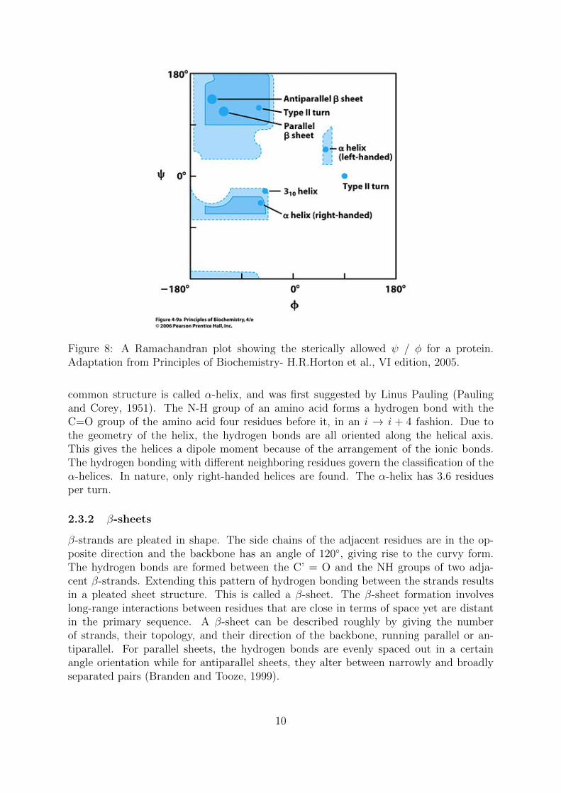
Figure 8: A Ramachandran plot showing the sterically allowed ψ / φ for a protein.Adaptation from Principles of Biochemistry- H.R.Horton et al., VI edition, 2005.

common structure is called α-helix, and was first suggested by Linus Pauling (Paulingand Corey, 1951). The N-H group of an amino acid forms a hydrogen bond with theC=O group of the amino acid four residues before it, in an i → i + 4 fashion. Due tothe geometry of the helix, the hydrogen bonds are all oriented along the helical axis.This gives the helices a dipole moment because of the arrangement of the ionic bonds.The hydrogen bonding with different neighboring residues govern the classification of theα-helices. In nature, only right-handed helices are found. The α-helix has 3.6 residuesper turn.

2.3.2 β-sheets

β-strands are pleated in shape. The side chains of the adjacent residues are in the op-posite direction and the backbone has an angle of 120◦, giving rise to the curvy form.The hydrogen bonds are formed between the C’ = O and the NH groups of two adja-cent β-strands. Extending this pattern of hydrogen bonding between the strands resultsin a pleated sheet structure. This is called a β-sheet. The β-sheet formation involveslong-range interactions between residues that are close in terms of space yet are distantin the primary sequence. A β-sheet can be described roughly by giving the numberof strands, their topology, and their direction of the backbone, running parallel or an-tiparallel. For parallel sheets, the hydrogen bonds are evenly spaced out in a certainangle orientation while for antiparallel sheets, they alter between narrowly and broadlyseparated pairs (Branden and Tooze, 1999).

10

2.3.3 Loops

The parts of the polypeptide connecting the well-defined alpha helices and beta sheetsare called loops and are typically less structured and flexible. The loops usually occuron the surface of the protein and frequently contain polar residues that interact withwater. Mutations in the loop regions are often tolerated since they do not break the coreof the protein. For instance, this might be used to alter the binding specificity. Hairpinloops are the units that connect two adjacent antiparallel β-sheets and are sometimessimply called turns. In small loops, a single cis-proline or glycine has been found to sta-bilize and promote the folding process. With the lack of a Cβ atom, glycine has a fasterrate of contact formation than other amino acids due to the increased backbone flexi-bility. Cis-proline contributes to a faster loop formation because of its largely restrictedconformational space arising from its cyclic side chain (Krieger et al., 2005).

Fig. 9 shows the various secondary structures discussed above. The coil is the α-helixand the arrow-heads represent a parallel β-sheet. These two are connected by the loops.

Figure 9: Structure of a mutant KcsA potassium channel with its secondary structures.PDBID: 1ZWI.

2.4 Elementary interactions in proteins

The sequence of a protein is believed to be solely responsible for the resulting nativestructure. Covalent bonds are formed by the interactions of electron pairs and are thestrongest chemical bond in a protein. The cysteine amino acids forming disulphide bonds,peptide bonds, and all bonds between atoms in the amino acids itself are all covalentinteractions. Several other elementary forces also play a major role in the folding process.Enthalpy contributes via the total interactions within the polypeptide chain.

11

2.4.1 Electrostatic forces

Non-covalent interactions are mostly interactions between charged ions. The electricpotential between two point charges, q1 and q2, at a distance r, is described by Coulomb’slaw

E =q1q24π�r

(1)

The Coulomb interactions are long-ranged as they decay as 1/r. The interaction ofq1 and q2 is repulsive for charges of the same sign, and attractive for opposite-sign ones.� is the absolute permittivity. Ionic bonds, between oppositely charged groups of aminoacids in close contact, are extremely favorable.

2.4.2 Van der Waals interactions

All atoms or molecules attract each other. Neutral atoms or molecules are made up ofcharged particles. The net cancellation of these charges present a neutral picture. Theattractive force generated by the shift of electrons towards another nucleus, results inpolarization of the charge. As two charges are brought nearer and nearer, the short-range repulsive force grows exponentially. The intermolecular attractive force is knownas Van der Waals interaction.

The long-range attraction decays as 1/r6. We can model the short-range repulsion by1/r12. 1/r12 can be obtained in a single multiplication once 1/r6 is available and is hencecheap to calculate.

Uij,LJ = 4�ij

��σij

rij

�12

−�σij

rij

�6�

(2)

where Uij,LJ is the Lennard-Jones potential for a pair of sites i and j separated by adistance rij. σij and �ij are Lennard-Jones parameters.

2.4.3 Hydrogen bonds

The pull of the electron towards a more electronegative atom along a bond will polarize thepair of atoms, and create a larger partial charge on the hydrogen. When this hydrogenis close to a different electronegative atom, we will get a hydrogen bond between twodifferent molecules due to the strong polarization of both. The energy of such a bondis around five kcal/mol and has short-range interaction. Charged side chain groups aremostly present on the surface of proteins and facing the aqueous phase. This leadsto hydrogen bonding with the medium, which also reduces the effective charge of suchgroups.

The C=O and N-H groups in polypeptide chains easily form hydrogen bonds. Inthe case of protein molecules in aqueous solution, amino acid residues would release twowater molecules, previously bound to them and form a hydrogen bond. Hydrogen bondsare common in the secondary structure of protein.

12

2.4.4 Entropy and free energy

Although all individual conformations are equally probable, there are lots of conforma-tions that are considered unfolded or unordered, but very few ordered conformations.Even if they were to have exactly the same enthalpy, this probability would factor in andmake it more likely to find the system unordered than ordered. Moving unordered toordered conformations is more unfavorable the higher the temperature is. It is possibleto show that the most favorable conformation is the one that minimizes the expressionof the free energy

F = E − TS, (3)

where F is the free energy, E is the energy and S is the entropy of the state at a giventemperature T.

The folding and unfolding reactions of a protein are governed by the entropy and thenon-covalent interactions (Zondlo, 2010). The hydrogen bonds have energies that are inthe range of 2-5 kcal/mol and Van der Waals interactions energies are approximately inthe range of 0.01 to 0.2 kcal/mol. The seemingly small values of energies adds up todirect the fate of the folding pathway. Small changes in pH or temperature can result indestruction of the secondary and tertiary structures of a folded structure of protein andis indicative of these weak non-covalent interactions.

2.5 Anfinsen’s dogma

Christian B. Anfinsen proposed that the native structure of a protein is determined solelyon the basis of its constituting amino acid sequence, for which he was awarded the NobelPrize in chemistry in 1972. He showed this by first fully denaturing an enzymatic protein,ribonuclease, containing 8 S-H groups. The mixture of products formed was inactive andretained the total count of disulphide bonds. When this process was reversed, usingthe products in the mixture, it converted into a homogeneous product, indistinguishablefrom native ribonuclease (Anfinsen, 1973). This led Anfinsen to postulate that at aspecific condition, such as temperature and pH, the protein adopts the structure with thelowest free energy. This is known as Anfinsen’s dogma (also called the thermodynamichypothesis).

2.6 Levinthal’s paradox

The polypeptide chain can fold into a protein, having a number of different conformations.The total number of possible conformations is of astronomical magnitude. Let us considera simple example - a protein of 100 amino acids having 99 peptide bonds. This will resultin 198 different degrees of freedom for its φ and ψ angles. Assuming three possible statesfor each angle, the total number of possible conformations is 3198. Even if nature couldsample each of these conformations in a matter of femtoseconds, the total time to exhaustall the possibilities would be more than the age of the universe!

In 1969, Cyrus Levinthal famously alluded to this by recognizing the fact that thoughproteins fold spontaneously and on a short time scale (in the order of milli/micro-seconds),the astronomical number of possible conformations of a polypeptide chain makes it a

13

paradox that folding into a protein still occurs (Levinthal, 1969). He suggested that theparadox can be resolved if the rapid formation of local interactions can guide and speedup the protein folding. The local amino acid sequences which form stable interactions canserve as nucleation points in the folding process (Levinthal, 1969). Levinthal suggested awell-defined kinetically controlled pathway to the native structure (Levinthal, 1968; Dilland Chan, 1997).

2.7 Protein Folding in vivo and in vitro

Protein folding is considered to be governed by long range interactions within a pro-tein (Ngo et al., 1994). Short-range interactions would not have resulted in such a hardand complex problem (Fraenkel, 1993; Unger and Moult, 1993). The free energy differ-ence between the unfolded, denatured state and the native structure is not more than theenergy of a hydrogen bond. This makes the folding process a precarious balance. Theheterogeneous contact combination of different residues in a polypeptide chain decides thefinal outcome of the folding process (Plotkin and Onuchic, 2000). The end result of thefolding process of the polymer chain is the lowest possible free energy state. The stabilityof the native folded protein is affected by the mutations of the amino acids (Zeldovich andShakhnovich, 2008; Onuchic et al., 1997). Mutations happen on a regular basis. Naturalselection disfavors mutations that negatively affect a protein’s function (Onuchic et al.,1997).

The polypeptide chains of amino acids that are longer than 100 residues have a ten-dency to fall back among themselves and form non-native aggregates (Brockwell andRadford, 2007). These are called folding intermediates. These intermediates can eitherbe kinetically stable enough that the non-native state needs to be reorganized throughsome mechanism or can be stepping stones on the path to reach the final native state.Biomolecules, classified as chaperonins, assist the process of folding the intermediatestep into the native state by binding to the unfolded, partially folded and misfoldedproteins (Evstigneeva et al., 2001).

Other kinetic factors such as incorrect disulphide bonds have the property to stabilizea structure due to the reduction in conformational entropy, i.e., the entropy arising fromdifferent conformations of the backbone. These kinetic factors can contribute against thefolding process towards the native structure. Protein folding is driven by entropy as wellas enthalpy. As mentioned above, the final resultant of the folding process is the lowestfree energy state. The energy landscape of this funnel is rough, since it contains multiplenon-native local minima. There are multiple minima separated by large barriers, definingthe meta-stable states (Fig. 10).

2.7.1 Experimental Techniques

Experimentally determining structures can be a time consuming process. The two mostcommon techniques used are X-ray crystallography and nuclear magnetic resonance (NMR).

X-ray crystallography is a method in which beams of X-rays collide on a crystal anddiffract in specific directions, based on the arrangement of atoms within the crystal. Apure protein in an aqueous solution precipitates and crystallizes under specific condi-tions such as pH, concentration of protein and temperature. A well-defined crystal of a

14

Figure 10: The energy landscape of protein folding.

protein will yield a high resolution picture of the spatial arrangement of the individualatoms (Chernov, 2003; Rupp and Wang, 2004). The limitation of this method lies in thedifficulty of forming the crystals. In addition, the picture obtained from this techniqueis just a single snapshot of a certain protein. Slightly different conditions can lead to adifference of as much as 1 A of the native structure between two snapshots of the samemolecule of protein.

NMR is based upon the magnetic spin behavior of the atomic nuclei of a molecule.Each nucleus of atoms experiences a unique chemical shift because of the specific chemicalenvironment when introduced in a magnetic field. The structure can be calculated byintroducing the molecule in a high-intensity magnetic field and studying these chemicalshifts. The biggest advantage this method has over X-ray crystallography is its ability tostudy the protein in the solvated state rather than as a crystal. The trade-off is that NMRresults in lower resolution of the protein. NMR studies also require a high concentrationof protein.

15

3 Protein Structure Prediction

3.1 Background and Methods

3.1.1 Bioinformatics

A term initially coined by Paulien Hogeweg and Ben Hesper in 1978 (Hogeweg, 1978);bioinformatics describes the comparative analysis of genome data by computational meth-ods (Hogeweg, 2011). This discipline has three key avenues of research: organizing bio-logical data in databases, analyze this data, and, perhaps the most important, extractingbiological importance out of the data (Luscombe et al., 2001).

There has been an explosion of biological data in the last couple of years (Choi et al.,2007; Reichhardt, 1999). As of April 2011, the NIH genetic sequence database Gen-Bank (Benson et al., 2008) has ∼ 135 million sequences mapped with more than 12.6billion bases, doubling every 18 month. Even if the present-day databases contain a sig-nificant amount of data, this is only the beginning. The pace of sequencing is increasingat a rate even modern computer technology has trouble to keep up with. The reasonis that the cost of sequencing has gone down considerably (Fig. 11). The first humangenome cost ∼ 3 billion USD. Now it is possible to sequence an individual human for afraction of that initial cost. This represents a fundamental challenge in bioinformatics;both from an analysis and a method development point of view.

Figure 11: In the last decade, the cost of DNA sequencing has fallen to a hundred-thousandth of its initial cost (Carr, 2010).

3.1.2 Alignment

A challenging question in molecular biology is to what extent a protein’s function canbe determined from its sequence, since proteins with high sequence identity frequently

16

have similar functions. It has been shown that above a threshold of around 50% residueidentity, the functional divergence is decreased dramatically (Sangar et al., 2007). Com-paring sequences becomes critical when doing evolutionary studies as well as functional orstructure predictions of proteins. In this comparison, it is common to find proteins of thesame family having positions or even a block of mutated residues. The goal of sequencealignment is to identify residues in two sequences that correspond to each other (Lesk,2002). Alignment algorithms measure the similarities by observing the patterns and vari-ations of conservation and draw conclusions about their evolutionary relationships andmutations between sequences (Mount, 2004). The sequences with high identity have obvi-ous functional similarities while the functional similarities for too low identity sequencesare very difficult to detect. When two sequences have more than 30% residue similarity,they are typically homologous. This range is known as the twilight zone (Rost, 1999).

We need to quantify the degree of biological relationships between sequences, aminoacids or nucleotides. The mutated amino acids can be substituted by amino acids ofsimilar or completely different chemical nature. The former is frequent, but the lattermuch rarer since it can affect the protein’s structure and function. To properly aligntwo sequences, we need a scoring method that takes this into account. It should be usedto account for the chemical nature of amino acids. The scoring matrix is on the aminoacid/nucleotide level. It gives values to represent the residue similarities. Two importantscoring matrices are PAM (Dayhoff et al., 1978) and BLOSUM (Henikoff and Henikoff,1992). Point Accepted Matrix or PAM was one of the first amino acid substitutionmatrix scoring methods. It was built by global alignment of sequences from 71 groupsof 34 superfamilies, with similarity above 85%. For each group, a phylogenetic tree isconstructed where the evolutionary distance of one PAM is equal to the probability of onepoint mutation per hundred residues. It is based on a Markov model where each changedepends on the current state, but not the history of previous states. The drawbacks ofPAM, in terms of assuming equal mutation rate for all amino acids in a sequence andan outdated dataset, makes BLOSUM a more attractive candidate for a scoring scheme.BLOcks SUbstitution Matrix or BLOSUM was developed using locally aligned proteinswith 62% and above identities. The probabilities of substitutions are calculated on blocksof conserved sequences.

Two historically important algorithms developed for alignment of sequences are theNeedleman-Wunsch algorithm (Needleman and Wunsch, 1970) and the Smith-Watermanalgorithm (Smith and Waterman, 1981). The Needleman-Wunsch algorithm comparesand tries to maximize the score based on residue-matching covering the entire length oftwo sequences. Comparison of all possible pairs of residues is called global alignment.This is mostly useful when the sequences are of similar lengths. The Smith-Watermanalgorithm compares local segments of the sequences, instead of extending the alignmentover the entire sequence. This method of comparison is called local alignment and isuseful in the case of varying length of the sequence having similar regions in them. Theonly essential difference is that the Needleman-Wunsch algorithm reports alignment cor-responding the maximum score over the whole sequence length and Smith-Watermanalgorithm reports the alignment corresponding to maximum subsequence.

17

Figure 12: Illustration of a multiple sequence alignment result for the first 40 residues ofhemoglobin using ClustalW (Thompson et al., 1994).

3.1.3 BLAST

Basic Local Alignment Search Tool or BLAST is a heuristic approach to the databasesearch problem (Altschul et al., 1990). It has revolutionized the identification of similarsequences in large databases and has been quoted as the paper with most citations in1990s (Taubs, 2000). Instead of comparing the query sequence with all sequence in thedatabase, BLAST splits the query sequence into a shorter word list and use this list toscan the database for hits. The database search results in a list of similar sequences,i.e. sequences with short word matches above a threshold. To get the individual residuesimilarity these hit are then realigned using the standard Smith-Waterman algorithm.The trick with BLAST is the word list. First, it is possible to pre-calculate a hash tablefor all word matches in the database to speed up the search. Second, the word list makesit possible to filter out many sequences with no similarity (no short word match) to thequery without the need for a full-fledged sequence alignment.

3.1.4 Multiple Sequence Alignment

The pair-wise sequence alignment often misses subtle similarities. It is important tohighlight the position conservation of residues as well as complex evolutionary divergentrelationships (Lobo, 2008). In the Multiple Sequence Aligment (MSA), the homologoussequences’ residues in a given column may have a common functional role (Edgar and Bat-zoglou, 2006). MSAs are able to identify a much more detailed and biologically relevantpicture of a protein family than single sequences. The representation of frequencies ofamino acids in a protein sequence of a family highlights the conserved residues (Gribskovand Veretnik, 1996). Conserved amino acid stretches have been widely used in proteinstructure prediction (Rost and Sander, 1994; Jones, 1999) and isolation of relevant regionsfacilitates a number of biological analyses (Attwood, 2002) (Fig 12).

18

3.1.5 Profiles

A profile is a representation of the multiple sequence alignment of all conserved regions.It creates a substitution matrix in which each position in a group of aligned sequence isassigned a score for each of the twenty possible amino acids.

Profile-sequence analysis is a method in which one queries a sequence against a profileof conserved regions in a multiple sequence alignment. This is more effective as profilesinherently have more information than a single sequence to compare with. Yet, replacingboth the target and template sequences with profiles has shown even more promises fordistantly related proteins that fall under the twilight zone (Rychlewski et al., 2000; Yonaand Levitt, 2002; Rychlewski et al., 2000).

3.1.6 PSI-BLAST

One powerful variant of profile-based methods builds frequency profiles using BLAST inits search and is called Position-Specific Iterated BLAST or PSI-BLAST (Altschul et al.,1997). The method of doing an initial search, constructing a profile from the hits ofthe search and then iterating this search based on the profile improves the sensitivity.PSI-BLAST constructs a multiple-sequence alignment with reference to a database byrunning BLAST, building a profile in its first step. This profile is used in place of theoriginal substitution matrix for a further search of the database to detect sequences usingprofile-sequence search. The newly detected sequences from this second round of thesearch, which are above the specified threshold, are again added to the alignment and theprofile is updated for another round of searching. A strength of PSI-BLAST is running asa start-to-finish program where one inputs the protein sequence and searches a database,with the resulting profile as a by-product after all the intermediate steps of alignment,scoring and iteration.

3.2 Structure Comparison

With the growing number of structures being determined, it is important to have meth-ods for comparing apparently similar three-dimensional structures. Homologous proteinssharing similar three-dimensional fold have evolved beyond sequence recognition. Struc-ture comparison is thus highly desirable and has therefore received considerable attentionfor many years (Shih and Hwang, 2003; Gibrat et al., 1996; Holm and Sander, 1996). Awide range of different quality measures is used in the literature to compare models struc-turally with the target. The aim is to quantify the correctness of the models comparedto the actual native structures. Some of the methods are given below.

3.2.1 RMSD

Root mean square deviation ( RMSD ) measures the similarity of the atomic coordinatesafter optimal superposition. It is mainly sensitive in identifying poorly modeled regionsof loops in a structure (Maiorov and Abagyan, 1997).

RMSD =

����(1/N)i=N�

i=1

δ2i , (4)

19

where δi is the distance between two positions for atom i and N is the number of pairsof equivalent atoms.

3.2.2 S-score

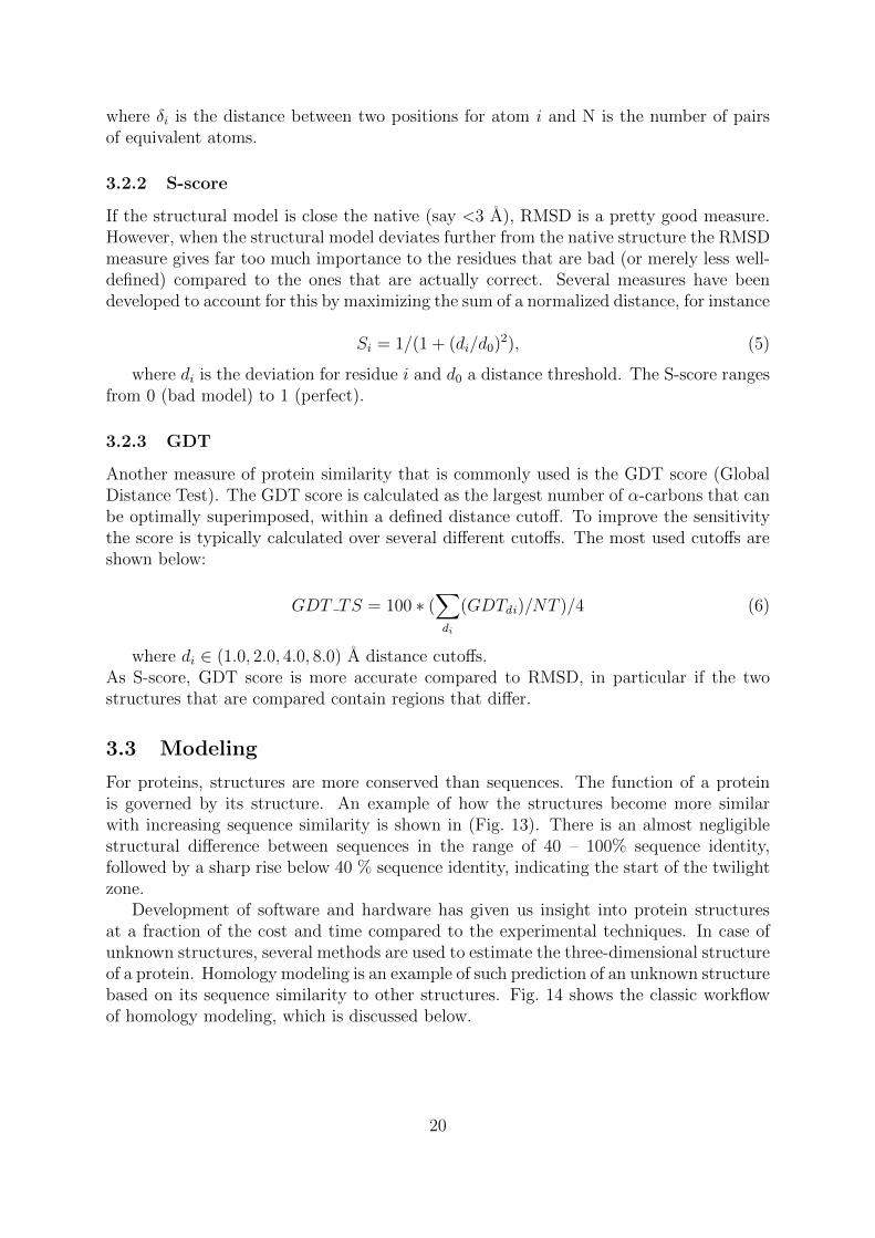
If the structural model is close the native (say <3 A), RMSD is a pretty good measure.However, when the structural model deviates further from the native structure the RMSDmeasure gives far too much importance to the residues that are bad (or merely less well-defined) compared to the ones that are actually correct. Several measures have beendeveloped to account for this by maximizing the sum of a normalized distance, for instance

Si = 1/(1 + (di/d0)2), (5)

where di is the deviation for residue i and d0 a distance threshold. The S-score rangesfrom 0 (bad model) to 1 (perfect).

3.2.3 GDT

Another measure of protein similarity that is commonly used is the GDT score (GlobalDistance Test). The GDT score is calculated as the largest number of α-carbons that canbe optimally superimposed, within a defined distance cutoff. To improve the sensitivitythe score is typically calculated over several different cutoffs. The most used cutoffs areshown below:

GDT TS = 100 ∗ (�

di

(GDTdi)/NT )/4 (6)

where di ∈ (1.0, 2.0, 4.0, 8.0) A distance cutoffs.As S-score, GDT score is more accurate compared to RMSD, in particular if the twostructures that are compared contain regions that differ.

3.3 Modeling

For proteins, structures are more conserved than sequences. The function of a proteinis governed by its structure. An example of how the structures become more similarwith increasing sequence similarity is shown in (Fig. 13). There is an almost negligiblestructural difference between sequences in the range of 40 – 100% sequence identity,followed by a sharp rise below 40 % sequence identity, indicating the start of the twilightzone.

Development of software and hardware has given us insight into protein structuresat a fraction of the cost and time compared to the experimental techniques. In case ofunknown structures, several methods are used to estimate the three-dimensional structureof a protein. Homology modeling is an example of such prediction of an unknown structurebased on its sequence similarity to other structures. Fig. 14 shows the classic workflowof homology modeling, which is discussed below.

20

Figure 13: A: Models with less than 30% sequence identity to the target frequentlyhave substantial alignment errors and a suboptimal template selection. B: Models with30-50% sequence identity to the target frequently have alignment errors in the non-conserved segments of the target protein, structural variation in templates, and incorrectreconstruction of the loops. C: Models having higher than 50% sequence identity to thetarget typically have the correct fold and the alignments tends to be mainly correct.

Figure 14: Flowchart of homology modeling. Courtesy of Dr. Bjorn Wallner.

21

3.3.1 Homology Modeling

Homology or comparative protein structure modeling constructs a three-dimensionalmodel of a given protein sequence based on its similarity to one or more known struc-tures (Jacobson and Sali, 2004). The minor changes in the sequence result in a smallchange in the structure. The most essential step in homology modeling is the alignmentof two or more sequences to determine whether they are homologous. It gives a verygood idea about the conserved regions and can identify the functional residues. One ofthe biggest factors to the success of homology modeling is the knowledge of almost allprotein folds. Today, 90% of the structures submitted to the PDB correspond to alreadyknown folds (Jinbo et al., 2004). This means that it is rare to find a completely newprotein which has no homologous sequence or folds known.

In reality though, it is not trivial to specify strict algorithms to identify homologousproteins at low levels of sequence identity. Hence, a database search to find a homologymatch of a protein does not always result in giving the best pair. Using information frommultiple templates can help improve the quality of homology models (Larsson et al.,2011).

3.3.2 Ab-intio

In the scenario where the target has no similarity to an already known protein struc-ture, the process resorted to is called ab-initio structure prediction. The aim of thisprocedure is to predict the structure of the protein and to apply physical principles tosearch through the various possible solutions. Ab-initio structure prediction requires alarge computational resource even for tiny proteins and methods like Folding@Home andRosetta@Home utilize distributed computing power to solve this problem.

The basic principle governing this method of structure prediction is that the nativeconfiguration of a protein molecule is the global free energy minima for the structure.However, as previously discussed, it is an exceptionally complicated search problem, asthe search space is gigantic to sample and to check all the possibilities is enormouslycomputationally expensive.

ROSETTA (Simons et al., 1999; Bonneau and Baker, 2001) assembles smaller frag-ments of known proteins and tries to assemble them using a Monte Carlo sampling ap-proach along with knowledge-based energy function. The reason for employing fragmentsin structure prediction is to reduce the complexity of the problem by reusing parts ofknown structures, which improves both performance and accuracy significantly. Suc-cessful ROSETTA predictions typically yield 3–6 A Cα RMSD models for 60-residueproteins (Rohl et al., 2004).

3.4 Model Quality Assessment of Protein Models

It is now easy to generate a large number of models in a short period of time. Therefore,it becomes critical to be able to judge and rank these models based on their quality.The first methods in the field, like ProsaII (Sippl, 1993), Verify3D (Luethy et al., 1992)and Errat, were developed as techniques to detect erroneous crystal structures. Thedevelopment of the R-free method (Brunger et al., 1987) has made these methods lessimportant for crystallography. There has since been a paradigm shift into now using

22

these methods for assessing the quality of protein models instead. This has also led tothe development of methods, Model Quality Assessment Programs (MQAPs), dedicatedto the prediction of protein model correctness.

Methods that only use information from a single model to assess the quality of amodel are called stand-alone methods. On the other hand, another genre of MQAPsgather predictions about a model’s quality from a range of different methods and thencompare the results. The basic idea behind such consensus analysis is that predictionsderived from a range of other methods should contain more information to compare andthat a better model will have many neighboring similar models and hence yield a higherscore. MQAPs using such consensus analysis are intuitively called consensus methods.These consensus MQAPs do not try to evaluate the quality of a model. Instead, they usethe similarity between a model and many other models. This type of evaluation is onlyuseful when there is a large set of models for the same target, which is typically the casein homology modeling.

3.4.1 ProQ

ProQ was the first method that used protein models instead of native structures, withdifferent similarity as a target function (Wallner and Elofsson, 2003). It is an exampleof a stand-alone method. ProQ uses neural networks to score models from a few basicstructural features such as atom contacts, exposed surface area, and predicted secondarystructure. This was subsequently combined with Pcons to improve the prediction evenfurther (Baker and Sali, 2001; Zhang, 2009). Pcons (Lundstom et al., 2001) was the firstconsensus method that predicted the quality of all models, by assigning a score to eachmodel reflecting the average similarity to the entire ensemble of models.

3.4.2 Global Quality and Local Quality of a Model

The scoring functions can be assigned on two levels. We can assign a single score whileassessing the model as a whole (global quality) or at residue level (local quality). Globalquality is beneficial in model selection processes since a single measure for each modelmakes it easy to qualitatively rank all models in a dataset. The importance of the localresidue level quality measure becomes more prominent when there are good regions in anaverage/low global quality model. This gives better insight into which part of the modelcan be trusted for making further improvements. Fig. 15 highlights the importance ofthe local quality measure in a model.

3.4.3 Importance of MQAP

After the rise of high throughput sequencing in 2004, it is now normal to produce mil-lions of sequences per day. A bottleneck thus becomes the determination of the three-dimensional structure from these sequences. Computational power has been rising rapidlyeach year and currently available methods can produce tens of thousands of model from asingle sequence in a day. It then becomes critical to have the ability to pick the best modelof these, which in an ideal world would be the native structure. Researchers around theglobe are trying to build faster and more accurate MQAPs to meet this growing demand.

23

0.0

1.0

2.0

3.0

4.0

0 50 100 150 200 250 300

dist

ance

dev

iatio

n (Å

)

position

!2-adrenergic G Protein-Coupled Receptor Model 1

T4 lysozyme

Apredicted deviation

true deviation

Figure 15: Predicted as well as true deviation for an early model of the β2-adrenergicreceptor. This GPCR model by Skolnick (Zhang et al., 2006) was published before anyexperimental structure was available, but ProQM correctly identifies regions where themodel was later found to deviate from the X-ray structure (Ray et al., 2010).

The challenge now is to build good models and choosing the correct one, quickly andaccurately, to complement the pace of high throughput sequencing.

3.5 CASP

Every second year since 1994, protein modelers test their methods in an internationalexperiment called Critical Assessment of Techniques for Protein Structure Prediction(CASP). Predictors in applied mathematics, computer science, biology, physics and chem-istry in well over 100 scientific centers around the world work for approximately threemonths to generate structure models for several tens of protein sequences selected bythe experiment organizers (Kryshtafovych and Fidelis, 2009). The proteins suggested forprediction (in the CASP language: targets) are either structures on the verge to be solvedor structures already solved and deposited in the PDB and withheld until the end of theCASP season. The categories in CASP 9 in 2010 involved tertiary structure predictionsfor template based modeling and free modeling for targets having no suitable templatesto use, refinement of models by performing finer corrections to get higher quality mod-els, identifying disordered regions detecting residue-residue contacts, function predictionand model quality assessment. CASP assesses the submitted models with GDT TS scorealong with a more sensitive scoring scheme, GDT-HA, which has smaller cutoffs for thedifferences.

24

4 Machine Learning Technique

4.1 Why teach a machine ?

Structure prediction of proteins can broadly be based on two methods. Physics-basedmethods assess a model based on the laws of physics and knowledge-based methods judgethe information of a model based on the rules of evolution. One of the most importantlessons from the previous rounds of CASP has been the large success of knowledge-basedprediction methods. Some of the more successful knowledge-based software involvedmethods of learning or extracting knowledge from the existing protein structures and toimplement this gained knowledge into predicting other unresolved structures (Larranagaet al., 2006). Machine learning techniques deal with pattern recognition, classification,and prediction, based on derived information from existing data (Tarca et al., 2007). Itis inherently an approximation of all the knowledge fed into the training and hence hasa limited accuracy.

Machine learning can successfully be used to classify models according to their quality.The core idea of machine learning is to train a program by showing it sets of good and badexamples, and subsequently use the trained program to predict other samples. Ideally,with an unknown model, the method should be able to classify it in either of the twocategories by statistical fitting of the unknown example to the examples the method wastrained on. The biggest strength of machine learning technique is that it is fast and thatno explicit relationships are needed beforehand.

There are two alternatives for the classification approach: supervised and unsuper-vised classification. In supervised classification, the dataset is divided into classes, whichare governed by the data’s characteristic or feature. The feature is a quantity that de-scribes an instance and is specific to a dataset (Kohavi and Provost, 1998). An exampleof features would be categorizing a dataset of human faces based on the features, suchas color, position of eyes and nose, or a dataset of different animals, differentiated by thevarious features such as habitat and size. The aim of the supervised classification problemis to accurately assign new members to different classes according to its features (Tarcaet al., 2007). This labeling of classes, before the classification of a data, indicates thesupervised learning. Contrary to this, in the unsupervised classification problem, a newdata discovers its own grouping without any pre-assigned class structure. The algorithmwould cluster similar featured data into classes based on certain similarities of attributes.Coming back to the previous example, a supervised classification would be when the an-imals of the animal dataset are assigned to a specific pre-assigned features, as the onesmentioned above. This is different in unsupervised classification, as the algorithm is letto study and classify the animals in the dataset. On inspection, we may find that onecluster of data is now based on the common sizes, while another one may be based onthe feature of color. Hence, the data found its own grouping.

4.2 Neural Networks

An artificial neural network is the attempt to mathematically model an algorithm thatmimics the human behavior of the brain to adapt and extract information (McCullochand Pitts, 1943). A neural network will have a component for recognition of a data

25

and another for classification, which are arranged in layers such that the output frommany connections, or nodes, is fed into a single node as input (Hirst and Sternberg, 1992;Presnell and Cohen, 1993; Rost, 1996; Rost and Sander, 1994; Larranaga et al., 2006;Rost, 2003). The network feeds an input in the input layer that feeds the informationto the hidden layer beneath it. In this hidden layer, nodes recode the information basedupon weight for error balancing and pass it on to the next hidden layer (if present). Ifthe information only flows forward, it is called a feed-forward network, while a feedbacknetwork also interacts between the nodes in a layer. Finally, the last hidden layer pushesthe result to the output layer.

4.3 Support Vector Machines

A Support Vector Machine (SVM) is a supervised technique which was introduced byVapnik in the late seventies (Vapnik, 1979). Conceptually, it non-linearly maps the inputvectors to a very high-dimensional feature space. In this feature space, the SVM tries toconstruct a linear plane for classification (Cortes and Vapnik, 1995). This network waslater extended to biological problems at the turn of the millennium (Hua and Sun, 2001;Cai et al., 2001) (Fig. 16).

Figure 16: Illustration of data from input space, represented in higher dimensional featurespace using kernels in the SVM.

The SVM is a mathematical model that classifies a set of samples into two classes.

26

The linear separation of these two classes has a decision margin. The distance betweena hyper plane, separating two classes, and the closest training samples to the decisionsurface is termed as the margin (Tarca et al., 2007). The dividing hyper plane can be oftwo-dimensional nature in its simplest form, though it is also possible to construct higher-dimensional planes. Kernels are developed with different mathematical representationsof the data points onto these higher-dimensional spaces. Linear, polynomial, and radialbasis function kernels are examples of common kernels used in a SVM to transform intohigher dimensions and are used for better classification. The sample points that arecrossed by these hyperplanes and are closest to maximum margin are called supportvectors.

By choosing a suitable basis function, the SVM can transform a non-linear probleminto a higher linear kernel space. The linear model in the feature space then corre-sponds to the non-linear model in the input space (Cover, 1965; Sewell, 2011). The easeof training and ability to scale to high-dimensional data makes the SVM a strong tool inmachine learning techniques (Markowetz, 2001). The major challenge though remains toidentify the appropriate kernel for perfect classification of the classes for a given applica-tion (Burges, 1998). New kernels are constantly developed to get a better fitting of thehyperplane in a complex feature space for classification.

27

5 Paper Summary

5.1 Model quality assessment for membrane proteins based onsupport vector machines (Paper 1)

Our long-standing goal is to predict the 3D structure of membrane proteins with highaccuracy to enable docking studies of proteins with unknown x-ray structures. Onestep in this direction is to be able to correctly identify and separate correct from lesscorrect models from a set of plausible models also known as model quality assessment.Further, it is also important to identify which regions of a protein model that are correctand incorrect. Several studies have focused on these issues but so far all of them haveexcluded membrane proteins. This is unfortunate since there is a huge gap between thefraction of membrane proteins in the genome (25%) and the membrane proteins in thestructural database (< 1%) making them an ideal target for computational approaches.In this study, we have improved and extended ProQ, one of the best methods for modelquality assessment of water-soluble proteins, to membrane proteins.

ProQM was the first model quality assessment program that was solely developed formembrane proteins. It was developed based on support vector machines with a linearkernel. With a systematic analysis of the features, sequence conservation together withprofile information showed the largest performance increase. This was expected as thesequence conservation and the profiles contain a large portion of information for thedescription of a protein structure.

Analysis of the results showed that the method was very good at detecting the residueswith less than 3 A deviation from the native structure residing in the membrane center.From the membrane core, the protein eventually becomes similar to globular domains.ProQM had a comparable performance to the current best globular MQAPs in thoseregions.

ProQM performed well while testing using the Skolnick set for GPCR proteins, over all15 models. We also attempted decoy selection on a large set of ROSETTA-generated low-resolution membrane protein decoys, we performed decoy selection test. The combinationof ProQM and ROSETTA showed seven-fold enrichment of the near-native decoys as thestarting population of decoys.

5.2 Support vector machine based model quality assessment forglobular proteins (Paper 2)

ProQ2 is a non-consensus based model quality assessment program for globular proteins.ProQ2 calculates structural properties based on the model and uses a SVM to predict thequality. The structural properties are similar to the ones used in the previous version ofProQ, but additional features that were shown to improve performance have been added.

The method uses a combination of features like evolutionary and multiple sequencealignment information along with other structural features to predict the local and globalquality of a model. All features are calculated over a sliding sequence window and thelocal structural quality is calculated by S-score. A global score is obtained by summingup the local scores and normalizing the value by dividing by the target length. Theprogram was trained by using a set of models generated in the 7th round of the CASP

28

experiment. Since it would be unfair to test the performance on the same data as usedfor training, scoring was instead performed on a similar dataset from CASP 8.

ProQ2 is significantly better than its predecessors at detecting high quality models,compared to the best single method in CASP8. The absolute quality assessment ofthe models at both local and global level is also improved. Combining ProQ2 with theconsensus method, Pcons, we improved the model selection even further, surpassing thebest servers presented in CASP 8.

29

6 Final thoughts

The protein structure prediction field has immense importance in drug design and struc-tural and functional studies. It is today easy to build large number of protein modelsfor any given sequence. Yet, we still lack the tools to consistently rank these modelsin order to select the best one. With more high throughput sequencing centers beingcreated globally, the number of sequences with unknown structures will increase. As aconsequence, the need for better model building and assessment methods will get in-creasingly important to bridge the gap between sequences with unknown structures vsexperimentally deduced structures.

The contacts between residues are important for maintaining the native fold. Pre-diction of these residue-residue contacts has been a challenging problem in structuralbioinformatics. Recently developed methods for accurate prediction of contacts will haveimplications in the field of fold recognition, ab initio protein folding, model quality assess-ment and de novo protein design (Jones et al., 2011). The successful methods extractedcorrelated mutation information from a MSA. In doing so, inherently, the methods showeda high tendency of false positives. This arose from the noise to the signal in the MSAbecause of the phylogenetic bias and the indirect coupling effect (Lapedes et al., 1999).The methods had a very low accuracy of around 20–40% in prediction (Grana et al., 2005;Hamilton et al., 2004; Fariselli et al., 2001; Jones et al., 2011). As recent as October 2011,there have been some ground breaking advances in the accuracy of these predictions (Mor-cos et al., 2011; Jones et al., 2011; Taylor et al., 2011). These new methods have shownvery promising results with high accuracies. PSICOV has shown an average precision ashigh as 80% when predicting residues separated by 5–9 positions. The methods, thoughquite promising, still have room for improvement. Since all the methods use MSA, thereis a need for better alignment tools to accurately align the tens of thousands of proteinsequences being found by all the advances in high throughput sequencing. Also, thesenew methods are heavily dependent on the extraction of coevolutionary information fromMSA. Hence, this is another aspect which needs further research.

30

7 Acknowledgment

First, I would like to thank Bjorn and Erik for believing in me. You have enrichedmy world with experiences, exposures and teachings. This was a dream come true and Ihave cherished every moment of it. Both of you inspire me each day to be better thanyesterday.

To the Lindahl group, I feel grateful for being in the perfect environment for meto learn and grow. Sander, for the times of being there as a mentor and as a friend.Rossen, for sharing the common love of Indian food and music! Szilard, for being myofficemate, with whom I have cherished many debates, for the past three years and beinga company in the numerous late working nights. Torben, for all the parties, debatesand venting we have shared. Sophie, for being there as a friend and a constant sourceof motivation.

Thank you Arne, for the numerous advices you gave me on bioinformatics. You havealways been an “unofficial” mentor to me.

I am immensely indebted to my friends who have walked beside me, all through thisjourney. Linnea, you have been my rock in the most challenging times, more thanonce. Marcin, for the countless brainstorming sessions, along with our many ”politicallyinappropriate” debates! Walter, for the numerous karaoke sessions and being a dearfriend.

It would be unfair on my part to not mention a few others who have been an integralpart of my life in Stockholm. Thank you to the Skwark family for the numerous foodyevenings and lovely company. Zak and Marion for always providing me a safe haven,away from the city buzz and for being a family to me. Maria, Lotta and Lollo forbeing more of a friend than a departmental component. I would also like to mentionStampen for giving me with the much needed distraction and relaxing evenings overthis period of time - you shall always remain as my second home.

Last, but most importantly, my parents and brother. Without you three, I would notbe where I am. The self-belief and standards that you have imbibed in me, shall alwaysbe my guide in life. The fire and will to stand against the general consensus has alwayspushed to me to go beyond. I will always remember to ‘never give up’... because youguys never gave up on me! This thesis I dedicate to you...

Arjun Ray, Stockholm, March 2012

31

List of Figures

1 A DNA codon consisting of three bases on the backbone of phosphate andsugar. . . . . . . . . . . . . . . . . . . . . . . . . . . . . . . . . . . . . . 1

2 The protein synthesis pathway. The DNA is expressed into the RNAthrough transcription process. The RNA is then translated into a pro-tein. . . . . . . . . . . . . . . . . . . . . . . . . . . . . . . . . . . . . . . 2

3 The mRNA copies in a complementary manner from the DNA. . . . . . . 34 The tRNA binds with the amino acids. . . . . . . . . . . . . . . . . . . . 35 The first tRNA links to the left-most codon of the mRNA strand in the

ribosome. . . . . . . . . . . . . . . . . . . . . . . . . . . . . . . . . . . . 36 The basic structure of an amino acid contains a carboxylic group, an amino

group and a side chain. . . . . . . . . . . . . . . . . . . . . . . . . . . . . 47 Fluid mosaic model of the cell membrane. Adaptation from Mind the

membrane (Pietzsch, 2004). . . . . . . . . . . . . . . . . . . . . . . . . . 68 A Ramachandran plot showing the sterically allowed ψ / φ for a protein.

Adaptation from Principles of Biochemistry- H.R.Horton et al., VI edition,2005. . . . . . . . . . . . . . . . . . . . . . . . . . . . . . . . . . . . . . 10

9 Structure of a mutant KcsA potassium channel with its secondary struc-tures. PDBID: 1ZWI. . . . . . . . . . . . . . . . . . . . . . . . . . . . . . 11

10 The energy landscape of protein folding. . . . . . . . . . . . . . . . . . . 1511 In the last decade, the cost of DNA sequencing has fallen to a hundred-

thousandth of its initial cost (Carr, 2010). . . . . . . . . . . . . . . . . . 1612 Illustration of a multiple sequence alignment result for the first 40 residues

of hemoglobin using ClustalW (Thompson et al., 1994). . . . . . . . . . . 1813 A: Models with less than 30% sequence identity to the target frequently

have substantial alignment errors and a suboptimal template selection. B:Models with 30-50% sequence identity to the target frequently have align-ment errors in the non-conserved segments of the target protein, structuralvariation in templates, and incorrect reconstruction of the loops. C: Mod-els having higher than 50% sequence identity to the target typically havethe correct fold and the alignments tends to be mainly correct. . . . . . 21

14 Flowchart of homology modeling. Courtesy of Dr. Bjorn Wallner. . . . . 2115 Predicted as well as true deviation for an early model of the β2-adrenergic

receptor. This GPCR model by Skolnick (Zhang et al., 2006) was pub-lished before any experimental structure was available, but ProQM cor-rectly identifies regions where the model was later found to deviate fromthe X-ray structure (Ray et al., 2010). . . . . . . . . . . . . . . . . . . . 24

16 Illustration of data from input space, represented in higher dimensionalfeature space using kernels in the SVM. . . . . . . . . . . . . . . . . . . 26

32

ReferencesAltschul, S., Gish, W., Miller, W., Myers, E., and Lipman, D. (1990). Basic local alignment search tool. Journal of molecular

biology, 215(3), 403–410.

Altschul, S., Madden, T., Schaffer, A., Zhang, J., Zhang, Z., Miller, W., and Lipman, D. (1997). Gapped BLAST and PSI-BLAST:a new generation of protein database search programs. Nucleic Acids Research, 25(17), 3389.

Anfinsen, C. B. (1973). Principles that govern the folding of protein chains. Science, 181(96), 223–230.

Attwood, T. (2002). The prints database: a resource for identification of protein families. Briefings in Bioinformatics, 3(3), 252.

Baker, D. and Sali, A. (2001). Protein structure prediction and structural genomics. Science, 294(5540), 93–96.

Barnhart, B. (1989). The department of energy (doe) human genome initiative. Genomics, 5, 657–660.

Bennett, M., Cox, A., and Leitch, I. (2004). Angiosperm DNA C-values database. Kew: Royal Botanic Gardens.

Benson, D., Karsch-Mizrachi, I., Lipman, D., Ostell, J., and Wheeler, D. (2008). Genbank. Nucleic acids research, 36(suppl 1),D25.

Bentley, S. and Parkhill, J. (2004). Comparative genomic structure of prokaryotes. Annual Review of Genetics, 38, 771–791.

Bonneau, R. and Baker, D. (2001). Ab initio protein structure prediction: progress and prospects. Annual Review of Biophysicsand Biomolecular Structure, 30, 173–189.

Bower, M., Cohen, F., and Dunbrack, R. (1997). Prediction of protein side-chain rotamers from a backbone-dependent rotamerlibrary: a new homology modeling tool. Journal of Molecular Biology, 267(5), 1268–1282.

Branden, C. and Tooze, J. (1999). Introduction to protein structure. Garland New York, 2nd edition.

Brigandt, I. (2002). Homology and the origin of correspondence. Biology and Philosophy, 17(3), 389–407.

Brigandt, I. and Griffiths, P. (2007). The importance of homology for biology and philosophy. Biology and Philosophy, 22(5),633–641.

Brockwell, D. and Radford, S. (2007). Intermediates: ubiquitous species on folding energy landscapes? Current Opinion inStructural Biology, 17(1), 30–37.

Brunger, A., Kuriyan, J., and Karplus, M. (1987). Crystallographic R factor refinement by molecular dynamics. Science, 235(4787).

Burges, C. (1998). A tutorial on support vector machines for pattern recognition. Data mining and knowledge discovery, 2(2),121–167.

Cai, Y., Liu, X., Xu, X., and Zhou, G. (2001). Support vector machines for predicting protein structural class. BMC Bioinfor-matics, 2(1), 3.

Carr, G. (2010). A special report on the human genome: Biology 2.0. The Economist.

Chernov, A. (2003). Protein crystals and their growth. Journal of Structural Biology, 142(1), 3–21.

Choi, C., Munch, R., Bunk, B., Barthelmes, J., Ebeling, C., Schomburg, D., Schobert, M., and Jahn, D. (2007). Combination ofa data warehouse concept with web services for the establishment of the pseudomonas systems biology database systomonas.Journal of Integrative Bioinformatics, 4(1).

Cortes, C. and Vapnik, V. (1995). Support-vector networks. Machine learning, 20(3), 273–297.

Cover, T. (1965). Geometrical and statistical properties of systems of linear inequalities with applications in pattern recognition.Electronic Computers, IEEE Transactions on, EC-14(3), 326–334.

Cullis, P. and De Kruijff, B. (1979). Lipid polymorphism and the functional roles of lipids in biological membranes. Biochimicaet Biophysica Acta (BBA)-Reviews on Biomembranes, 559(4), 399–420.

Davies, J. and Rubinsztein, D. (2006). Polyalanine and polyserine frameshift products in Huntington’s disease. Journal of MedicalGenetics, 43(11), 893.

Dayhoff, M., Schwartz, R., and Orcutt, B. (1978). Atlas of protein sequence and structure, volume 5, chapter A model ofevolutionary change in proteins., pages 345–352. National Biomedical Research Foundation, Silver Spring, Maryland.

De Beer, S. (1971). Homology, an unsolved problem, volume 11. Oxford University Press.

33

Dill, K. and Chan, H. (1997). From Levinthal to pathways to funnels. Nature Structural Biology, 4(1), 10–19.

Donoghue, M. (1994). Keywords in evolutionary biology, chapter Homology, pages 170–179. Harvard University Press, Cambridge,MA.

Dunbrack, R. (2002). Rotamer libraries in the 21st century. Current Opinion in Structural Biology, 12(4), 431–440.

Dunbrack, R. and Karplus, M. (1994). Conformational analysis of the backbone-dependent rotamer preferences of proteinsidechains. Nature Structural & Molecular Biology, 1(5), 334–340.

Edgar, R. and Batzoglou, S. (2006). Multiple sequence alignment. Current Opinion in Structural Biology, 16(3), 368–373.

Evstigneeva, Z., Solov’eva, N., and Sidel’nikova, L. (2001). Structures and functions of chaperones and chaperonins (review).Applied Biochemistry and Microbiology, 37(1), 1–13.

Fariselli, P., Olmea, O., Valencia, A., and Casadio, R. (2001). Prediction of contact maps with neural networks and correlatedmutations. Protein Engineering, 14(11), 835.

Fitch, W. and Margoliash, E. (1970). The usefulness of amino acid and nucleotide sequences in evolutionary studies. EvolutionaryBiology, 4, 67–109.

Fraenkel, A. (1993). Complexity of protein folding. Bulletin of Mathematical Biology, 55(6), 1199–1210.

Friedman, S. and Weinstein, I. (1965). Fidelity in protein synthesis: proline miscoding in a thermophile system. Biochemical andBiophysical Research Communications, 21(4), 339.

Gibrat, J., Madej, T., and Bryant, S. (1996). Surprising similarities in structure comparison. Current Opinion in StructuralBiology, 6(3), 377–385.

Grana, O., Baker, D., MacCallum, R. M., Meiler, J., Punta, M., Rost, B., Tress, M. L., and Valencia, A. (2005). CASP6 assessmentof contact prediction. Proteins: Structure, Function, and Bioinformatics, 61, 214–224.

Gribskov, M. and Veretnik, S. (1996). Identification of sequence patterns with profile analysis. Methods in Enzymology, 266,198–211.

Hamilton, N., Burrage, K., Ragan, M., and Huber, T. (2004). Protein contact prediction using patterns of correlation. Proteins:Structure, Function, and Bioinformatics, 56(4), 679–684.

Henikoff, S. and Henikoff, J. (1992). Amino acid substitution matrices from protein blocks. Proceedings of the National Academyof Sciences of the United States of America, 89(22), 10915–10919.

Hirst, J. and Sternberg, M. (1992). Prediction of structural and functional features of protein and nucleic acid sequences byartificial neural networks. Biochemistry, 31(32), 7211–7218.

Hogeweg, P. (1978). Simulating the growth of cellular forms. Simulation, 31(3), 90.

Hogeweg, P. (2011). The roots of bioinformatics in theoretical biology. PLoS Computational Biology, 7(3).

Holm, L. and Sander, C. (1996). Mapping the protein universe. Science, 273(5275), 595.

Hua, S. and Sun, Z. (2001). Support vector machine approach for protein subcellular localization prediction. Bioinformatics,17(8), 721.

Jacobson, M. and Sali, A. (2004). Comparative protein structure modeling and its applications to drug discovery. Annual reportsin Medicinal Chemistry, 39, 259–276.

Jakob, R. and Schmid, F. (2008). Energetic coupling between native-state prolyl isomerization and conformational protein folding.Journal of Molecular Biology, 377(5), 1560–1575.

Jinbo, X., Libo, Y., and Ming, L. (2004). Consensus fold recognition by predicted model quality. Master’s thesis, University ofWaterloo.

Jones, D. (1999). Protein secondary structure prediction based on position–specific scoring matrices. J Mol Biol, 292(2), 195–202.

Jones, D., Buchan, D., Cozzetto, D., and Pontil, M. (2011). PSICOV: Precise structural contact prediction using sparse inversecovariance estimation on large multiple sequence alignments. Bioinformatics.

Kendrew, J., Bodo, G., Dintzis, H., Parrish, R., Wyckoff, H., and Phillips, D. (1958). A three-dimensional model of the myoglobinmolecule obtained by X-ray analysis. Nature, 181, 662–666.

Kohavi, R. and Provost, F. (1998). Glossary of terms. Machine Learning, 30(June), 271–274.

34

Kooyman, G. and Ponganis, P. (1998). The physiological basis of diving to depth: birds and mammals. Annual Review ofPhysiology, 60(1), 19–32.

Krieger, F., Moglich, A., and Kiefhaber, T. (2005). Effect of proline and glycine residues on dynamics and barriers of loop formationin polypeptide chains. Journal of the American Chemical Society, 127(10), 3346–3352.

Kryshtafovych, A. and Fidelis, K. (2009). Protein structure prediction and model quality assessment. Drug Discovery Today,14(7), 386–393.

Lander, E., Linton, L., Birren, B., Nusbaum, C., Zody, M., Baldwin, J., Devon, K., Dewar, K., Doyle, M., FitzHugh, W., et al.(2001). Initial sequencing and analysis of the human genome. Nature, 409(6822), 860–921.

Lapedes, A., Giraud, B., Liu, L., and Stormo, G. (1999). Correlated mutations in models of protein sequences: phylogenetic andstructural effects. Proceedings of the AMS/SIAM Conference on Statistics in Molecular Biology, pages 236–256.

Larranaga, P., Calvo, B., Santana, R., Bielza, C., Galdiano, J., Inza, I., Lozano, J., Armananzas, R., Santafe, G., Perez, A., andRobles, V. (2006). Machine learning in bioinformatics. Briefings in Bioinformatics, 7(1), 86–112.

Larsson, P., Skwark, M., Wallner, B., and Elofsson, A. (2011). Improved predictions by pcons. net using multiple templates.Bioinformatics, 27(3), 426.

Lesk, A. (2002). Introduction to bioinformatics. Oxford University Press, 1st edition.

Levinthal, C. (1968). Are there pathways for protein folding? Journal of Medical Physics, 65(1), 44–45.

Levinthal, C. (1969). How to fold graciously. Mossbauer spectroscopy in biological systems, pages 22–24.

Linderstrøm-Lang, K. (1952). Lane Medical Lectures: Proteins and Enzymes. Stanford University Press.

Lobo, I. (2008). Basic local alignment search tool (BLAST). Nature Education, 1(1).

Luckey, M. (2008). Membrane Structural Biology. With Biochemical and Biophysical Foundations. Cambridge University press,1st edition.

Luethy, R., Bowie, J., and Eisenberg, D. (1992). Assessment of protein models with three–dimensional profiles. Nature, 356(6364),283–85.

Lundstom, J., Rychlewski, L., Bujnicki, J., and Elofsson, A. (2001). Pcons: a neural-network-based consensus predictor thatimproves fold recognition. Protein Science, 10(11), 2354–2362.

Luscombe, N., Greenbaum, D., and Gerstein, M. (2001). What is bioinformatics? An introduction and overview. Yearbook ofMedical Informatics, pages 83–100.

Madiraju, S. M. and Poitout, V. (2007). GPCRs and Insulin Secretion: 119 and Counting. Endocrinology, 148(6)(6), 2598–2600.

Maiorov, V. and Abagyan, R. (1997). A new method for modeling large-scale rearrangements of protein domains. ProteinsStructure Function and Genetics, 27(3), 410–424.

Markowetz, F. (2001). Support vector machines in bioinformatics. Master’s thesis, University of Heidelberg.

Mathieu, S., Poteau, R., and Trinquier, G. (2008). Estimating the “Steric Clash” at cis Peptide Bonds. The Journal of PhysicalChemistry B , 112(26), 7894–7902.

McCulloch, W. and Pitts, W. (1943). A logical calculus of the ideas immanent in nervous activity. Bulletin of MathematicalBiology, 5(4), 115–133.

Morcos, F., Pagnani, A., Lunt, B., Bertolino, A., Marks, D., Sander, C., Zecchina, R., Onuchic, J., Hwa, T., and Weigt, M.(2011). Direct-coupling analysis of residue co-evolution captures native contacts across many protein families. Proceedings ofthe National Academy of Sciences.

Moss, G. (1996). Basic terminology of stereochemistry (IUPAC Recommendations 1996). Pure and Applied Chemistry, 68(12),2193–2222.

Mount, D. W. (2004). Bioinformatics: sequence and genome analysis. CSHL press.

Needleman, S. and Wunsch, C. (1970). A general method applicable to the search for similarities in the amino acid sequence oftwo proteins. Journal of Molecular Biology, 48(3), 443–453.

Ngo, J., Marks, J., and Karplus, M. (1994). Computational complexity, protein structure prediction, and the Levinthal paradox.In The Protein Folding Problem and Tertiary Structure Prediction., pages 435–508, Boston. Birkhauser.

35

Onuchic, J., Luthey-Schulten, Z., and Wolynes, P. (1997). Theory of protein folding: the energy landscape perspective. Annualreview of physical chemistry, 48(1), 545–600.

Pauling, L. and Corey, R. (1951). Configurations of polypeptide chains with favored orientations around single bonds: two newpleated sheets. Proceedings of the National Academy of Sciences of the United States of America, 37(11), 729.

Pietzsch, J. (2004). Mind the membrane. A living frontier–exploring the dynamics of the cell membrane.

Plotkin, S. and Onuchic, J. (2000). Investigation of routes and funnels in protein folding by free energy functional methods.Proceedings of the National Academy of Sciences of the United States of America, 97(12), 6509.

Presnell, S. and Cohen, F. (1993). Artificial neural networks for pattern recognition in biochemical sequences. Annual Review ofBiophysics and Biomolecular Structure, 22(1), 283–298.

Ramachandran, G., Ramakrishnan, C., and Sasisekharan, V. (1963). Stereochemistry of polypeptide chain configurations. Journalof Molecular Biology, 7, 95.

Ray, A., Lindahl, E., and Wallner, B. (2010). Model quality assessment for membrane proteins. Bioinformatics, 26(24), 3067.

Reichhardt, T. (1999). It’s sink or swim as a tidal wave of data approaches. Nature, 399(6736), 517–520.

Rohl, C., Strauss, C., Misura, K., and Baker, D. (2004). Protein structure prediction using rosetta. Methods in enzymology, 383,66–93.

Rost, B. (1996). PHD: predicting 1 dimensional protein structure by profile based neural networks. Methods in enzymology, 266,525–539.

Rost, B. (1999). Twilight zone of protein sequence alignments. Protein engineering, 12(2), 85.

Rost, B. (2003). Neural networks predict protein structure: hype or hit? In Artificial intelligence and heuristic methods inbioinformatics, volume 183, pages 34–50, Tokyo. NATO Advanced Study Institute on Artificial Intelligence and HeuristicMethods in Bioinformatics, IOS Press.

Rost, B. and Sander, C. (1994). Combining evolutionary information and neural networks to predict protein secondary structure.Proteins-Structure Function and Genetics, 19(1), 55–72.

Rupp, B. and Wang, J. (2004). Predictive models for protein crystallization. Methods, 34(3), 390–407.

Rychlewski, L., Li, W., Jaroszewski, L., and Godzik, A. (2000). Comparison of sequence profiles. strategies for structural predictionsusing sequence information. Protein Science, 9(2), 232–241.

Sangar, V., Blankenberg, D., Altman, N., and Lesk, A. (2007). Quantitative sequence-function relationships in proteins based ongene ontology. BMC Bioinformatics, 8(1), 294.

Schrauber, H., Eisenhaber, F., and Argos, P. (1993). Rotamers: To be or not to be?: An analysis of amino acid side-chainconformations in globular proteins. Journal of Molecular Biology, 230(2), 592–612.

Sewell, M. (2011). svm kernel. http://www.svms.org/kernels/.

Shih, E. and Hwang, M. (2003). Protein structure comparison by probability-based matching of secondary structure elements.Bioinformatics, 19(6), 735.

Simons, K., Bonneau, R., Ruczinski, I., and Baker, D. (1999). Ab initio protein structure predictions of CASP III targets usingROSETTA. Proteins, Suppl 3, 171–176.

Singer, S. and Nicolson, G. (1972). The fluid mosaic model of the structure of cell membranes. Science, 175(23), 720–731.

Sippl, M. (1993). Recognition of errors in three–dimensional structures of proteins. Proteins, 17(4), 355–362.

Smith, T. and Waterman, M. (1981). Identification of common molecular subsequences. Journal of Molecular Biology, 147(1),195–197.

Stein, R. (1993). Mechanism of enzymatic and nonenzymatic prolyl cis-trans isomerization. Advances in protein chemistry, 44,1–24.

Suzuki, Y., Oishi, K., Nakano, H., and Nagayama, T. (1987). A strong correlation between the increase in number of prolineresidues and the rise in thermostability of five bacillus oligo-1, 6-glucosidases. Applied microbiology and biotechnology, 26(6),546–551.

Tanford, C. (1980). The Hydrophobic Effect: Formation of Micelles and Biological Membranes, volume 233. Wiley New York,2nd edition.

36

Tarca, A., Carey, V., Chen, X., Romero, R., and Draghici, S. (2007). Machine learning and its applications to biology. PLoScomputational biology, 3(6), e116.

Taubs, G. (2000). Sense from sequences: Stephen F. Altschul on bettering BLAST. Science Watch, 11, 3–4.

Taylor, W., Jones, D., and Sadowski, M. (2011). Protein topology from predicted residue contacts. Protein Science.

Thompson, J., Higgins, D., and Gibson, T. (1994). CLUSTAL W: improving the sensitivity of progressive multiple sequencealignment through sequence weighting, positions-specific gap penalties and weight matrix choice. Nucleic Acids Research,22(22), 4673–4680.

Unger, R. and Moult, J. (1993). Finding the lowest free energy conformation of a protein is an NP-hard problem: Proof andimplications. Bulletin of Mathematical Biology, 55(6), 1183–1198.

Vapnik, V. (1979). Restoration of Dependences from Empirical Data. Translated from the Russian by Samuel Kotz. Springer,NewYork.

Vauquelin, L. and Robiquet, P. (1806). The discovery of a new plant principle in asparagus sativus. Annales de Chimie, 57,88–93.

Wallner, B. and Elofsson, A. (2003). Can correct protein models be identified? Protein Science, 12(5), 1073–1086.

Waterston, R., Lindblad-Toh, K., Birney, E., Rogers, J., Abril, J., Agarwal, P., Agarwala, R., Ainscough, R., Alexandersson, M.,An, P., et al. (2002). Initial sequencing and comparative analysis of the mouse genome. Nature, 420(6915), 520–562.

Yona, G. and Levitt, M. (2002). Within the twilight zone: a sensitive profile-profile comparison tool based on information theory.Journal of Molecular Biology, 315(5), 1257–1275.

Zeldovich, K. and Shakhnovich, E. (2008). Understanding protein evolution: from protein physics to Darwinian selection. AnnualReview of Physical Chemistry, 59, 105–127.

Zhang, Y. (2009). Protein structure prediction: when is it useful? Current Opinion in Structural Biology, 19(2), 145–155.

Zhang, Y., Devries, M. E., and Skolnick, J. (2006). Structure modeling of all identified G protein-coupled receptors in the humangenome. PLoS Computational Biology, 2(2), e13.

Zimmer, C. (2009). On the origin of eukaryotes. Science, 325(5941), 666.

Zondlo, N. (2010). Non-covalent interactions: Fold globally, bond locally. Nature Chemical Biology, 6(8), 567–568.

37