Library of Congress Cataloging-in-Publication Data · Garcia San Jose State University Pren tice Hall, Upp er Saddle Riv er, New Jersey 07458. Library of Congress Cataloging-in-Publication

Second Edition

Numerical Methods for Physics

Alejandro L. Garcia

San Jose State University

Prentice Hall, Upper Saddle River, New Jersey 07458

Library of Congress Cataloging-in-Publication Data

Garcia, Alejandro L.,Numerical methods for physics / Alejandro L. Garcia. { 2nd ed.p. cm.

Includes bibliographical references and index.ISBN 0-13-906744-21. Mathematical physics. 2. Di�erential equations,

Partial{Numerical solutions. 3. Physics{Data processing. I.Title.

QC20 .G37 2000530.15{dc21

99-28552CIP

Executive Editor: Alison ReevesEditor-in-Chief: Paul F. CoreyAssistant Vice President of Production and Manufacturing: David W. RiccardiExecutive Managing Editor: Kathleen SchiaparelliAssistant Managing Editor: Lisa KinneProduction Editor: Linda DeLorenzoMarketing Manager: Steven SartoriEditorial Assistant: Gillian BuonannoManufacturing Manager: Trudy PisciottiArt Director: Jayne ConteCover Designer: Bruce KenselaarCover Art: John Christiana

c 2000, 1994 by Prentice-Hall, Inc.Upper Saddle River, New Jersey 07458

MATLAB(R) is a registered trademark of The MathWorks, Inc.

All rights reserved. No part of this book may be reproduced, in any form or by any means,without permission in writing from the publisher.

Printed in the United States of America

10 9 8 7 6 5 4 3 2 1

ISBN 0-13-906744-2

Prentice-Hall International (UK) Limited, LondonPrentice-Hall of Australia Pty. Limited, SydneyPrentice-Hall Canada Inc., TorontoPrentice-Hall Hispanoamericana, S.A., Mexico

Prentice-Hall of India Private Limited, New Delhi

Prentice-Hall of Japan, Inc., TokyoPrentice-Hall (Singapore) Pte LtdEditora Prentice-Hall do Brasil, Ltda., Rio de Janeiro

Contents

Preface v

1 Preliminaries 1

1.1 PROGRAMMING . . . . . . . . . . . . . . . . . . . . . . . . . . 11.2 BASIC ELEMENTS OF MATLAB . . . . . . . . . . . . . . . . . 31.3 BASIC ELEMENTS OF C++ . . . . . . . . . . . . . . . . . . . 101.4 PROGRAMS AND FUNCTIONS . . . . . . . . . . . . . . . . . 161.5 NUMERICAL ERRORS . . . . . . . . . . . . . . . . . . . . . . . 26

2 Ordinary Di�erential Equations I:

Basic Methods 37

2.1 PROJECTILE MOTION . . . . . . . . . . . . . . . . . . . . . . 372.2 SIMPLE PENDULUM . . . . . . . . . . . . . . . . . . . . . . . . 46

3 Ordinary Di�erential Equations II:

Advanced Methods 67

3.1 ORBITS OF COMETS . . . . . . . . . . . . . . . . . . . . . . . 673.2 RUNGE-KUTTA METHODS . . . . . . . . . . . . . . . . . . . . 743.3 ADAPTIVE METHODS . . . . . . . . . . . . . . . . . . . . . . . 813.4 *CHAOS IN THE LORENZ MODEL . . . . . . . . . . . . . . . 86

4 Solving Systems of Equations 107

4.1 LINEAR SYSTEMS OF EQUATIONS . . . . . . . . . . . . . . . 1074.2 MATRIX INVERSE . . . . . . . . . . . . . . . . . . . . . . . . . 1164.3 *NONLINEAR SYSTEMS OF EQUATIONS . . . . . . . . . . . 122

5 Analysis of Data 141

5.1 CURVE FITTING . . . . . . . . . . . . . . . . . . . . . . . . . . 1415.2 SPECTRAL ANALYSIS . . . . . . . . . . . . . . . . . . . . . . . 1535.3 *NORMAL MODES . . . . . . . . . . . . . . . . . . . . . . . . . 163

6 Partial Di�erential Equations I:

Foundations and Explicit Methods 191

6.1 INTRODUCTION TO PDEs . . . . . . . . . . . . . . . . . . . . 1916.2 DIFFUSION EQUATION . . . . . . . . . . . . . . . . . . . . . . 195

iii

iv CONTENTS

6.3 *CRITICAL MASS . . . . . . . . . . . . . . . . . . . . . . . . . . 202

7 Partial Di�erential Equations II:

Advanced Explicit Methods 215

7.1 ADVECTION EQUATION . . . . . . . . . . . . . . . . . . . . . 2157.2 *PHYSICS OF TRAFFIC FLOW . . . . . . . . . . . . . . . . . 225

8 Partial Di�erential Equations III:

Relaxation and Spectral Methods 249

8.1 RELAXATION METHODS . . . . . . . . . . . . . . . . . . . . . 2498.2 *SPECTRAL METHODS . . . . . . . . . . . . . . . . . . . . . . 258

9 Partial Di�erential Equations IV:

Stability and Implicit Methods 279

9.1 STABILITY ANALYSIS . . . . . . . . . . . . . . . . . . . . . . . 2799.2 IMPLICIT SCHEMES . . . . . . . . . . . . . . . . . . . . . . . . 2879.3 *SPARSE MATRICES . . . . . . . . . . . . . . . . . . . . . . . . 294

10 Special Functions and Quadrature 309

10.1 SPECIAL FUNCTIONS . . . . . . . . . . . . . . . . . . . . . . . 30910.2 BASIC NUMERICAL INTEGRATION . . . . . . . . . . . . . . 31810.3 *GAUSSIAN QUADRATURE . . . . . . . . . . . . . . . . . . . 325

11 Stochastic Methods 341

11.1 KINETIC THEORY . . . . . . . . . . . . . . . . . . . . . . . . . 34111.2 RANDOM NUMBER GENERATORS . . . . . . . . . . . . . . . 34711.3 DIRECT SIMULATION MONTE CARLO . . . . . . . . . . . . 35611.4 *NONEQUILIBRIUM STATES . . . . . . . . . . . . . . . . . . . 365

Bibliography 399

Selected Solutions 407

Index 418

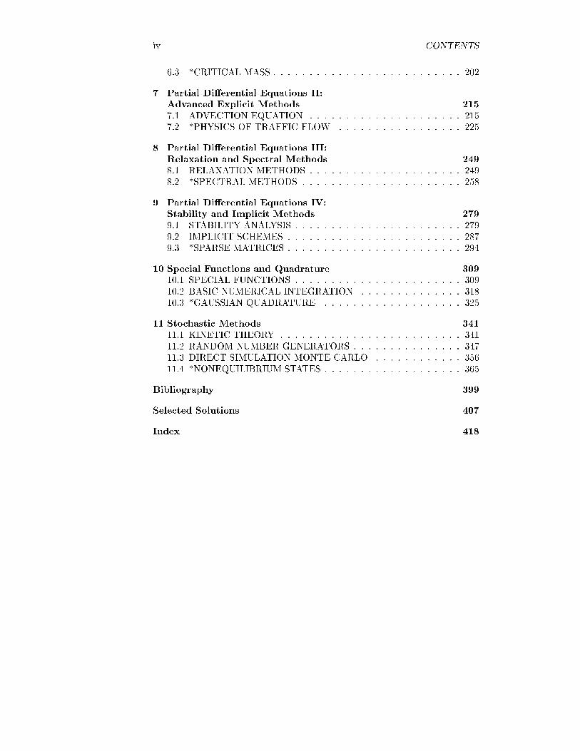
Preface

When I was an undergraduate, computers were just beginning to be introducedinto the university curriculum. Physics majors were expected to take a singlesemester of Pascal taught by the computer science department. We wrote pro-grams to sort lists, process a payroll, and so forth, but were expected to acquirethe specialized tools of scienti�c computing on our own. Most of us wastedmany human and computer hours learning them by trial and error.

In recent years, many departments have added a computational physicscourse, taught by physicists, to their curricula. However, there is still con-siderable debate as to how this course should be organized. My philosophy isto use the upper division/graduate mathematical physics course as a model.Consider the following parallels between this text and a typical math physicsbook: A variety of numerical and analytical techniques used in physics are cov-ered. Topics include ordinary and partial di�erential equations, linear algebra,Fourier transforms, integration, and probability. Because the text is written forphysicists, these techniques are applied to solving realistic problems, many ofwhich the students have encountered in other courses.

Numerical Methods for Physics is organized to cover what I believe are themost important, basic computational methods for physicists. The structureof the book di�ers considerably from the generic numerical analysis text. Forexample, about a third of the book is devoted to partial di�erential equations.This emphasis is natural considering the fundamental importance of Maxwell'sequations, the Schr�odinger equation, the Boltzmann equation, and so forth.Chapters 6 and 7 introduce some methods in computational uid dynamics, anincreasingly important topic in the �elds of nonlinear physics, environmentalphysics, and astrophysics.

Numerical techniques may be classi�ed as basic, advanced, and cutting edge.On the whole, this text covers only fundamental techniques; to work e�ectivelywith advanced numerical methods requires that the user �rst understand thebasic algorithms. The discussion in the \Beyond This Chapter" section at theend of each chapter guides the reader to advanced algorithms and indicateswhen it is appropriate to use them. Unfortunately, the cutting edge moves soquickly that any attempt to summarize the latest algorithms would quickly beout of date.

The material in this text may be arranged in various ways to suit anythingfrom a 10-week, upper-division class to a full-semester, graduate course. Most

v

vi PREFACE

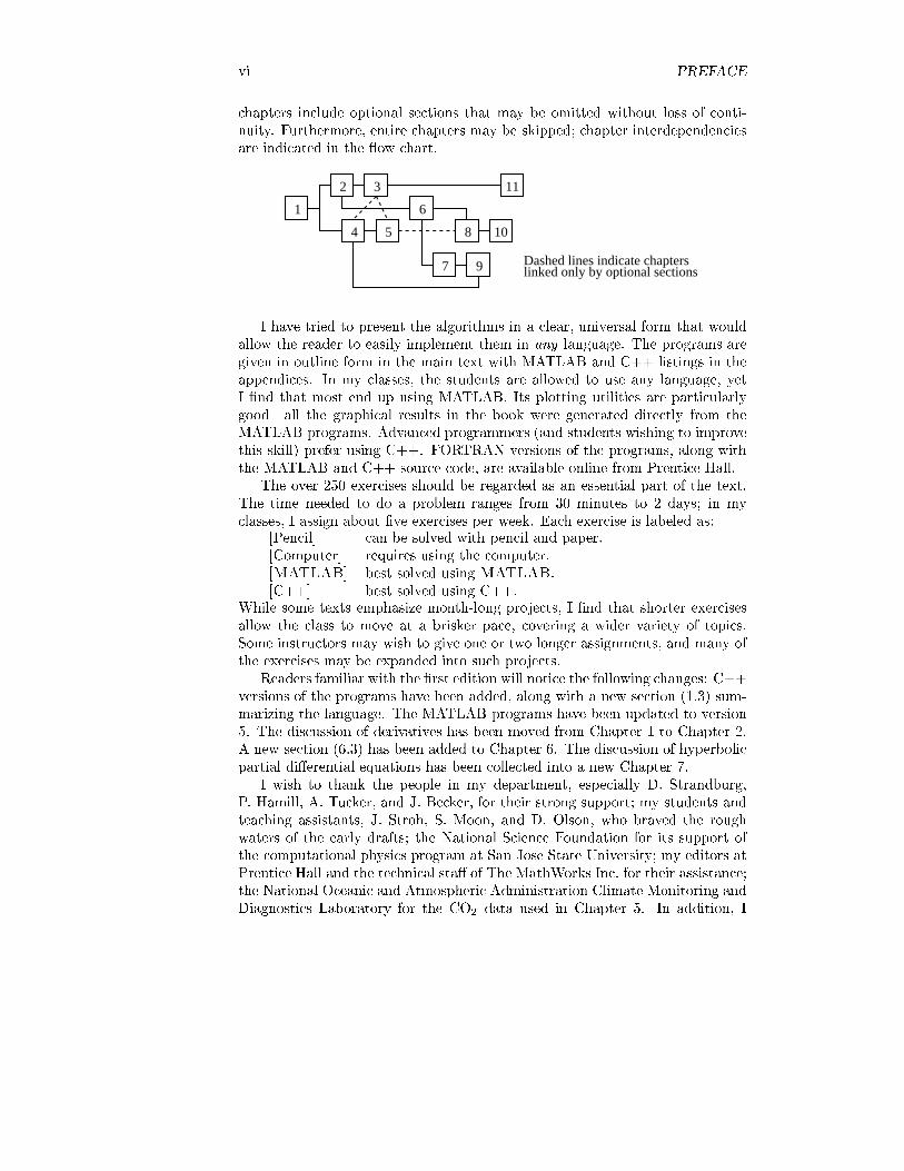
chapters include optional sections that may be omitted without loss of conti-nuity. Furthermore, entire chapters may be skipped; chapter interdependenciesare indicated in the ow chart.

1

2 3

4 5

6

7

8

9

10

11

Dashed lines indicate chapterslinked only by optional sections

I have tried to present the algorithms in a clear, universal form that wouldallow the reader to easily implement them in any language. The programs aregiven in outline form in the main text with MATLAB and C++ listings in theappendices. In my classes, the students are allowed to use any language, yetI �nd that most end up using MATLAB. Its plotting utilities are particularlygood|all the graphical results in the book were generated directly from theMATLAB programs. Advanced programmers (and students wishing to improvethis skill) prefer using C++. FORTRAN versions of the programs, along withthe MATLAB and C++ source code, are available online from Prentice Hall.

The over 250 exercises should be regarded as an essential part of the text.The time needed to do a problem ranges from 30 minutes to 2 days; in myclasses, I assign about �ve exercises per week. Each exercise is labeled as:

[Pencil] can be solved with pencil and paper.[Computer] requires using the computer.[MATLAB] best solved using MATLAB.[C++] best solved using C++.

While some texts emphasize month-long projects, I �nd that shorter exercisesallow the class to move at a brisker pace, covering a wider variety of topics.Some instructors may wish to give one or two longer assignments, and many ofthe exercises may be expanded into such projects.

Readers familiar with the �rst edition will notice the following changes: C++versions of the programs have been added, along with a new section (1.3) sum-marizing the language. The MATLAB programs have been updated to version5. The discussion of derivatives has been moved from Chapter 1 to Chapter 2.A new section (6.3) has been added to Chapter 6. The discussion of hyperbolicpartial di�erential equations has been collected into a new Chapter 7.

I wish to thank the people in my department, especially D. Strandburg,P. Hamill, A. Tucker, and J. Becker, for their strong support; my students andteaching assistants, J. Stroh, S. Moon, and D. Olson, who braved the roughwaters of the early drafts; the National Science Foundation for its support ofthe computational physics program at San Jose State University; my editors atPrentice Hall and the technical sta� of The MathWorks Inc. for their assistance;the National Oceanic and Atmospheric Administration Climate Monitoring andDiagnostics Laboratory for the CO2 data used in Chapter 5. In addition, I

PREFACE vii

appreciate the comments of the following reviewers: David A. Boness, SeattleUniversity; Wolfgang Christian, Davidson College; David M. Cook, LawrenceUniversity; Harvey Gould, Clark University; Cleve Moler, The MathWorks, Inc;Cecile Penland, University of Colorado, Boulder; and Ross L. Spencer, BrighamYoung University. Finally, I owe a special debt of gratitude to my entire familyfor their moral support as I wrote this book.

Alejandro L. Garcia

Dedicated to

Jose�na Ovies Garc��a

and

Miriam Gonz�alez L�opez

The programs in this book have been included for their instructional value. Although

every e�ort has been made to ensure that they are error free, neither the author nor

the publisher shall be held responsible or liable for any damage resulting in connection

with or arising from the use of any of the programs in this book.

7.2. *PHYSICS OF TRAFFIC FLOW 225

program to use this scheme and compare it with the others discussed in this section

for the cases shown in Figures 7.3{7.7. For what values of � is it stable? [Computer]

7.2 *PHYSICS OF TRAFFIC FLOW

Fluid Mechanics

In uid mechanics the equations of motion are obtained by constructing equa-tions of the form

@p

@t= �r �F(p) (7.29)

or in one dimension,@p

@t= � @

@xF (p) (7.30)

Here p is any one of the conserved quantities

p =

8<:

mass densityx; y or z�momentum densityenergy density

(7.31)

and F is

F (p) =

8<:

mass uxx; y or z�momentum uxenergy ux

(7.32)

that is, the corresponding ux.While the equations for the momentum and energy are somewhat compli-

cated, the equation for the mass density, �, is quite simple. The mass ux equalsthe mass density times the uid velocity, v, so

@�(x; t)

@t= � @

@xf�(x; t)v(x; t)g (7.33)

This equation is known as the equation of continuity. The equation for themomentum density may be rewritten as an equation for the velocity. Thisvelocity equation involves the energy density (the coupling is in the pressureterm), so we must solve the entire set of equations simultaneously.

The full set of hydrodynamics equations is called the Navier-Stokes equa-

tions. For a variety of reasons, these equations are usually not solved in theirfull form but rather with a number of approximations. Of course the approxima-tions used depend on the problem at hand. For example, air is incompressibleto a good approximation in many subsonic ows.

TraÆc Flow

One of the simplest, nontrivial ows that may be studied involves uids forwhich the velocity is only a function of density,

v(x; t) = v(�) (7.34)

226 CHAPTER 7. PDES II: ADVANCED EXPLICIT METHODS

For example, suppose that the velocity of the uid decreased linearly with in-creasing density as

v(�) = vm(1� �=�m) (7.35)

where vm > 0 is the maximum velocity and �m > 0 is the maximum density.What type of uid behaves this way? One ow you are probably very familiarwith is automobile traÆc. The maximum velocity is the speed limit; if thedensity is near zero (few cars on the road), then the traÆc moves at this speed.The maximum density, �m, is achieved when the traÆc is bumper-to-bumper.While on real highways the ow may not exactly obey Equation (7.35), it turnsout to be a good �rst approximation.[65]

Our equation for the evolution of the density may be written as

@�

@t= � @

@x

�(� +

1

2��)�

�(7.36)

where � = vm and � = �2vm=�m. This equation is called the generalizedinviscid Burger's equation. We obtain the standard inviscid Burger's equationwhen � = 0 and � = 1. This equation has been studied extensively because itis the simplest nonlinear PDE with wave solutions.[16] Equations of this typeappear frequently in nonlinear acoustics and shock wave theory.

Returning to our traÆc model, we want to develop a method to solve thenonlinear PDE,

@�

@t= � @

@xf�v(�)g (7.37)

Rewrite this equation as

@�

@t= �

�d

d��v(�)

�@�

@x(7.38)

or@�

@t= �c(�)@�

@x(7.39)

where c(�) � d(�v)=d�. Using our linear function for v(�) as given by Equation(7.35), we have

c(�) = vm(1� 2�=�m) (7.40)

Notice that c(�) is also linear in � and takes the values c(0) = vm and c(�m) =�vm. The function c(�) is not the speed of the traÆc, but rather is the speedat which disturbances (or waves) in the ow will travel. Since c(�) may be bothpositive or negative, the waves may move in either direction. Note, however,that c(�) � v(�), so the waves may never move faster than the cars.

Method of Characteristics

For c(�) = constant, we have the advection equation for which we alreadyknow the solution. We may build an analytical solution to (7.39) from ourknowledge of the solution of the advection equation by using the method of


x

t

x1 x2

Characteristic line

Slope = 1/c

ρ(x,t)

= ρ 0(x 1

)

ρ(x,t)

= ρ 0(x 2

)

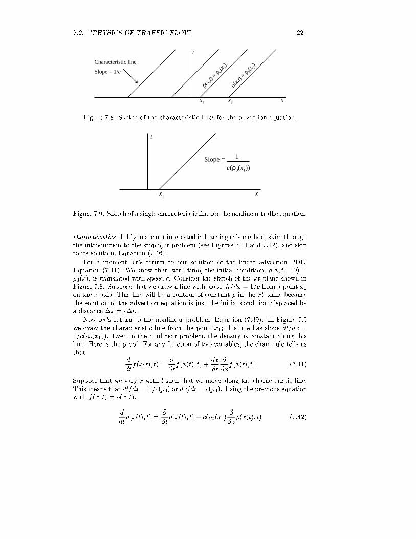
Figure 7.8: Sketch of the characteristic lines for the advection equation.

x

t

x1

Slope = 1

c(ρ0(x1))

Figure 7.9: Sketch of a single characteristic line for the nonlinear traÆc equation.

characteristics .[1] If you are not interested in learning this method, skim throughthe introduction to the stoplight problem (see Figures 7.11 and 7.12), and skipto its solution, Equation (7.46).

For a moment let's return to our solution of the linear advection PDE,Equation (7.11). We know that, with time, the initial condition, �(x; t = 0) =�0(x), is translated with speed c. Consider the sketch of the xt plane shown inFigure 7.8. Suppose that we draw a line with slope dt=dx = 1=c from a point x1on the x-axis. This line will be a contour of constant � in the xt plane becausethe solution of the advection equation is just the initial condition displaced bya distance �x = c�t.

Now let's return to the nonlinear problem, Equation (7.39). In Figure 7.9we draw the characteristic line from the point x1; this line has slope dt=dx =1=c(�0(x1)). Even in the nonlinear problem, the density is constant along thisline. Here is the proof: For any function of two variables, the chain rule tells usthat

d

dtf(x(t); t) =

@

@tf(x(t); t) +

dx

dt

@

@xf(x(t); t) (7.41)

Suppose that we vary x with t such that we move along the characteristic line.This means that dt=dx = 1=c(�0) or dx=dt = c(�0). Using the previous equationwith f(x; t) = �(x; t),

d

dt�(x(t); t) =

@

@t�(x(t); t) + c(�0(x))

@

@x�(x(t); t) (7.42)


x

t

x1

Slope = 1

c(ρ0(x1))

x2

Slope = 1

c(ρ0(x2))

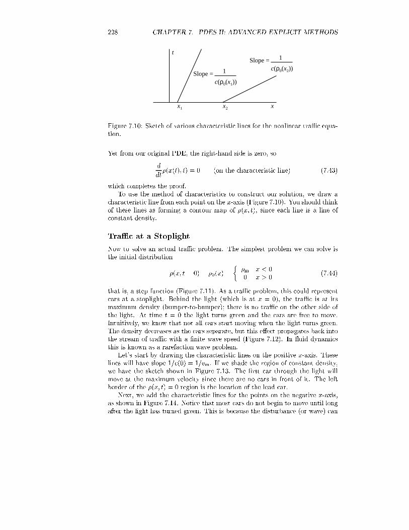
Figure 7.10: Sketch of various characteristic lines for the nonlinear traÆc equa-tion.

Yet from our original PDE, the right-hand side is zero, so

d

dt�(x(t); t) = 0 (on the characteristic line) (7.43)

which completes the proof.To use the method of characteristics to construct our solution, we draw a

characteristic line from each point on the x-axis (Figure 7.10). You should thinkof these lines as forming a contour map of �(x; t), since each line is a line ofconstant density.

TraÆc at a Stoplight

Now to solve an actual traÆc problem. The simplest problem we can solve isthe initial distribution

�(x; t = 0) = �0(x) =

��m x < 00 x > 0

(7.44)

that is, a step function (Figure 7.11). As a traÆc problem, this could representcars at a stoplight. Behind the light (which is at x = 0), the traÆc is at itsmaximum density (bumper-to-bumper); there is no traÆc on the other side ofthe light. At time t = 0 the light turns green and the cars are free to move.Intuitively, we know that not all cars start moving when the light turns green.The density decreases as the cars separate, but this e�ect propagates back intothe stream of traÆc with a �nite wave speed (Figure 7.12). In uid dynamicsthis is known as a rarefaction wave problem.

Let's start by drawing the characteristic lines on the positive x-axis. Theselines will have slope 1=c(0) = 1=vm. If we shade the region of constant density,we have the sketch shown in Figure 7.13. The �rst car through the light willmove at the maximum velocity since there are no cars in front of it. The leftborder of the �(x; t) = 0 region is the location of the lead car.

Next, we add the characteristic lines for the points on the negative x-axis,as shown in Figure 7.14. Notice that most cars do not begin to move until longafter the light has turned green. This is because the disturbance (or wave) can


x

ρ0(x)

ρ = 0

ρ = ρm

Figure 7.11: Initial density pro�le for traÆc at a stoplight.

TAXI

FISH

x = 0

t = 0

TAXI

FISH

t > 0

Figure 7.12: TraÆc moving after a stoplight turns green. Notice that in thesecond frame the last car toward the rear has not moved.

x

t

ρ(x,t) = 0

Figure 7.13: Partial construction of �(x; t) in the xt plane using characteristiclines. In the shaded region the density �(x; t) is zero. The left boundary of thisregion is given by the position of the lead car.


x

t

ρ(x,t) = 0ρ(x,t) = ρm

Figure 7.14: Partial construction of �(x; t) in the xt plane using characteristiclines. In the shaded region on the left the density �(x; t) is maximum (bumper-to-bumper).

x

t

ρ(x,t) = 0ρ(x,t) = ρm

x = εx = −ε

Figure 7.15: Characteristic lines for a continuous initial density pro�le. Thisdensity pro�le goes to a step function as �! 0.

only move with velocity c(�m). For our linear relation between v and �, we havec(�m) = �vm.

To obtain all the characteristic lines we must remember that our initialcondition is discontinuous. Suppose that we modi�ed �0(x) so that it variedcontinuously from �m to zero in a neighborhood of radius � about x = 0. Theslopes of the characteristic lines in this neighborhood would vary continuouslyfrom 1=vm to �1=vm (Figure 7.15).

Taking the limit � ! 0, we have our �nal picture of the characteristic lines

Expansion Fan

x

t

ρ(x,t) = 0ρ(x,t) = ρm

Figure 7.16: Construction of �(x; t) in the xt plane using characteristic lines.


x

ρ(x,t)t1t2

t2 > t1 > 0Lead car

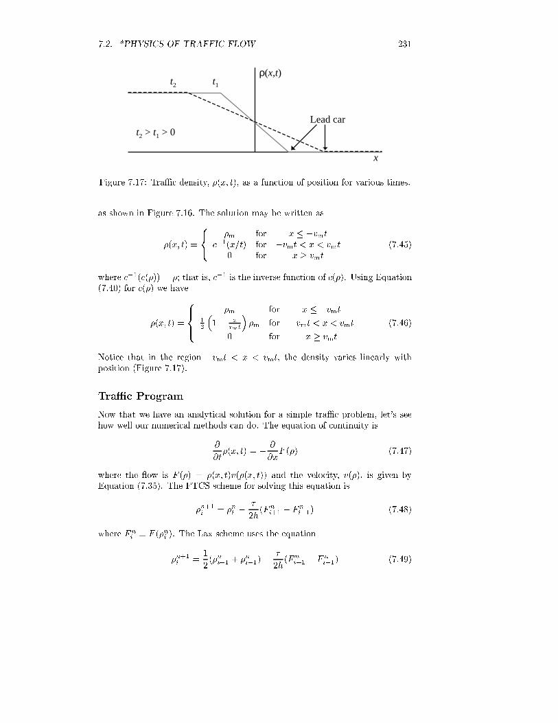
Figure 7.17: TraÆc density, �(x; t), as a function of position for various times.

as shown in Figure 7.16. The solution may be written as

�(x; t) =

8<:

�m for x � �vmtc�1(x=t) for �vmt < x < vmt

0 for x � vmt(7.45)

where c�1(c(�)) = �; that is, c�1 is the inverse function of c(�). Using Equation(7.40) for c(�) we have

�(x; t) =

8><>:

�m for x � �vmt12

�1� x

vmt

��m for �vmt < x < vmt

0 for x � vmt

(7.46)

Notice that in the region �vmt < x < vmt, the density varies linearly withposition (Figure 7.17).

TraÆc Program

Now that we have an analytical solution for a simple traÆc problem, let's seehow well our numerical methods can do. The equation of continuity is

@

@t�(x; t) = � @

@xF (�) (7.47)

where the ow is F (�) = �(x; t)v(�(x; t)) and the velocity, v(�), is given byEquation (7.35). The FTCS scheme for solving this equation is

�n+1i = �ni ��

2h(Fn

i+1 � Fni�1) (7.48)

where Fni � F (�ni ). The Lax scheme uses the equation

�n+1i =1

2(�ni+1 + �ni�1)�

�

2h(Fn

i+1 � Fni�1) (7.49)


Table 7.2: Outline of program traffic, which computes the equation of conti-nuity for traÆc ow.

� Select numerical parameters (� , h, etc.).

� Set initial condition (7.52) and periodic boundary conditions.

� Initialize plotting variables.

� Loop over desired number of steps.

{ Compute the ow, F (�) = �(x; t)v(�(x; t)).

{ Compute new values of density using:

� FTCS scheme (7.48) or;

� Lax scheme (7.49) or;

� Lax-Wendro� scheme (7.50).

{ Record density for plotting.

{ Display snap-shot of density versus position. [MATLAB only]

� Graph density versus position and time as mesh plot.

� Graph contours of density versus position and time.

See pages 240 and 244 for program listings.

Finally, the Lax-Wendro� scheme uses

�n+1i = �ni ��

2h(Fn

i+1 � Fni�1) +

�2

2

1

h

�ci+ 1

2

Fni+1 � Fn

i

h� ci� 1

2

Fni � Fn

i�1

h

�(7.50)

where

ci� 12� c(�ni� 1

2

); �ni� 12

� �ni�1 + �ni2

(7.51)

Notice how the last term of (7.50) is built: We would like to be able to evaluatethe function c(�) at values between grid points, that is, at i + 1

2 and i � 12 .

Since we know the value of � only at grid points, we estimate its value betweengrid points by using a simple average. We use this estimated value for �i� 1

2to

evaluate ci� 12.

The program called traffic, which implements these numerical schemes, isoutlined in Table 7.2. As an initial condition we take a square pulse of the form

�(x; t = 0) = �0(x) =

��m �L=4 < x < 00 otherwise

(7.52)

This initial value problem is similar to the stoplight problem considered above


ρ(x,t) = 0

ρ = ρm

Shock front

ρ = 0

x−L/2 −L/4 L/2

t

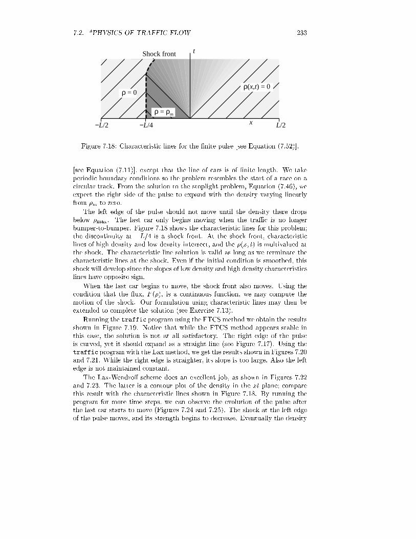
Figure 7.18: Characteristic lines for the �nite pulse [see Equation (7.52)].

[see Equation (7.11)], except that the line of cars is of �nite length. We takeperiodic boundary conditions so the problem resembles the start of a race on acircular track. From the solution to the stoplight problem, Equation (7.46), weexpect the right side of the pulse to expand with the density varying linearlyfrom �m to zero.

The left edge of the pulse should not move until the density there dropsbelow �max. The last car only begins moving when the traÆc is no longerbumper-to-bumper. Figure 7.18 shows the characteristic lines for this problem;the discontinuity at �L=4 is a shock front. At the shock front, characteristiclines of high density and low density intersect, and the �(x; t) is multivalued atthe shock. The characteristic line solution is valid as long as we terminate thecharacteristic lines at the shock. Even if the initial condition is smoothed, thisshock will develop since the slopes of low density and high density characteristicslines have opposite sign.

When the last car begins to move, the shock front also moves. Using thecondition that the ux, F (�), is a continuous function, we may compute themotion of the shock. Our formulation using characteristic lines may then beextended to complete the solution (see Exercise 7.13).

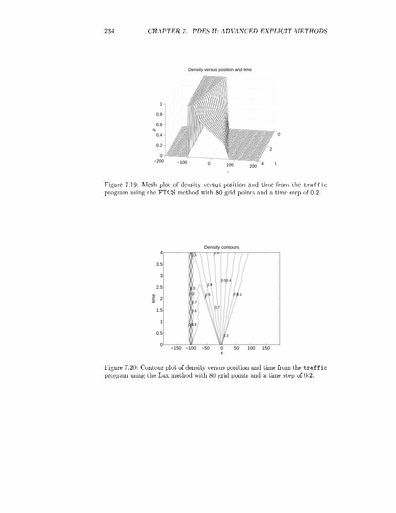
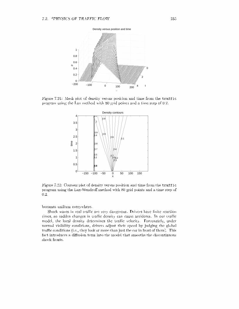
Running the traffic program using the FTCS method we obtain the resultsshown in Figure 7.19. Notice that while the FTCS method appears stable inthis case, the solution is not at all satisfactory. The right edge of the pulseis curved, yet it should expand as a straight line (see Figure 7.17). Using thetraffic program with the Lax method, we get the results shown in Figures 7.20and 7.21. While the right edge is straighter, its slope is too large. Also the leftedge is not maintained constant.

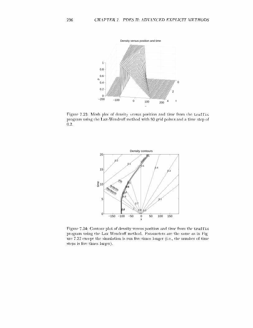
The Lax-Wendro� scheme does an excellent job, as shown in Figures 7.22and 7.23. The latter is a contour plot of the density in the xt plane; comparethis result with the characteristic lines shown in Figure 7.18. By running theprogram for more time steps, we can observe the evolution of the pulse afterthe last car starts to move (Figures 7.24 and 7.25). The shock at the left edgeof the pulse moves, and its strength begins to decrease. Eventually the density


0

2

4−200 −100 0 100 200

0

0.2

0.4

0.6

0.8

1

t

x

Density versus position and time

ρ

Figure 7.19: Mesh plot of density versus position and time from the traffic

program using the FTCS method with 80 grid points and a time step of 0.2.

−150 −100 −50 0 50 100 1500

0.5

1

1.5

2

2.5

3

3.5

4

0.1

0.10.2 0.2

0.3

0.3

0.4

0.4

0.5

0.5

0.6

0.6

0.70.7

0.8

0.8

0.91

x

time

Density contours

Figure 7.20: Contour plot of density versus position and time from the trafficprogram using the Lax method with 80 grid points and a time step of 0.2.


0

2

4−200 −100 0 100 200

0

0.2

0.4

0.6

0.8

1

t

x


ρ


program using the Lax method with 80 grid points and a time step of 0.2.

−150 −100 −50 0 50 100 1500

0.5

1

1.5

2

2.5

3

3.5

4 0.1

0.1

0.2 0.2

0.3

0.3

0.4

0.4

0.50.5

0.6

0.6

0.7

0.7

0.8

0.8

0.90.9

1

x

time

Density contours

Figure 7.22: Contour plot of density versus position and time from the trafficprogram using the Lax-Wendro� method with 80 grid points and a time step of0.2.

becomes uniform everywhere.

Shock waves in real traÆc are very dangerous. Drivers have �nite reactiontimes, so sudden changes in traÆc density can cause accidents. In our traÆcmodel, the local density determines the traÆc velocity. Fortunately, undernormal visibility conditions, drivers adjust their speed by judging the globaltraÆc conditions (i.e., they look at more than just the car in front of them). Thisfact introduces a di�usion term into the model that smooths the discontinuousshock fronts.


0

2

4−200 −100 0 100 200

0

0.2

0.4

0.6

0.8

1

t

x


ρ


program using the Lax-Wendro� method with 80 grid points and a time step of0.2.

−150 −100 −50 0 50 100 1500

5

10

15

20

0

0000

0

0

0

0

0

0

0

0

0

0

0

0

00

000

00000

00

0.1

0.1

0.1

0.2

0.2

0.2

0.3

0.3

0.4

0.4

0.5

0.5

0.6

0.7

0.8

0.8

0.9

0.9

1

x

time

Density contours

Figure 7.24: Contour plot of density versus position and time from the trafficprogram using the Lax-Wendro� method. Parameters are the same as in Fig-ure 7.22 except the simulation is run �ve times longer (i.e., the number of timesteps is �ve times larger).


0

10

20−200 −100 0 100 200

0

0.2

0.4

0.6

0.8

1

t

x


ρ


program using the Lax-Wendro� method. The contour plot for this run is shownin Figure 7.24.

EXERCISES

7. The ow of traÆc is F (x; t) = �(x; t)v(�). For the stoplight problem, obtain an

expression for F (x; t) using the solution (7.46) and v(�) = vm(1��=�m). Sketch F (x; t)versus x for t > 0, and show that it is maximum at x = 0 (i.e., at the light). [Pencil]

8. Call xc(t) the position of a given car; then

dxcdt

= v(�(xc(t); t)) (7.53)

(a) Show that

xc(t) =

�xc(0) t < �xc(0)=vm

vmt� 2p�xc(0)vmt t > �xc(0)=vm (7.54)

by using the solution to the stoplight problem, Equation (7.46). [Pencil] (b) Plot the

trajectories xc in the xt plane for various xc(0). [Computer] (c) Plot the time it takes

for a car to reach the intersection as a function of jxc(0)j. [Computer]

9. After a time t, the total amount of traÆc that has passed through the light isN(t) =R10�(x; t)dx. Show that N(t) =

R t0F (x = 0; t) dt, where F (x; t) = �(x; t)v(x; t) is the

ow. [Pencil]

10. Modify the traffic program so that it uses a Gaussian pulse of width L=4 as an

initial distribution for the density. Center the pulse at x = 0 with �(0; 0) = �m. Show

how the density evolves with time. Explain why one side of the pulse expands while

the other contracts [remember that the wave speed, c(�), is not a constant]. Describe

what a driver on this racetrack will experience. [Computer]


11. Modify the traffic program so that it uses the initial condition

�(x; t = 0) =�m2[1 + cos(4�x=L)]

(a) Plot the density versus position for a variety of times and show that the cosine wave

turns into a sawtooth wave. In nonlinear acoustics this is referred to as an N-wave.

If you have ever been to a very loud rock concert, you may have heard one of these.

(b) Modify your program to compute the spatial power spectrum of the density (see

Section 5.2). Remove the zero wave number component. Initially, the spectrum will

contain a single peak, but in time other peaks appear. Use a mesh plot to graph the

spectrum versus wave number and time. [Computer]12. Suppose that we have a uniform density of traÆc with a small congested area.Modify the traffic program so that it uses the initial condition

�(x; t = 0) = �0[1 + � exp(�x2=2�2)]

where � = 1=5, � = L=8, and �0 are a constants. (a) Show that for light traÆc

(e.g., �0 = �m=4) the perturbation moves forward. What is its speed? (b) Show that

for heavy traÆc (e.g., �0 = 3�m=4) the perturbation moves backward. Interpret this

result physically. (c) Show that for �0 = �m=2 the perturbation is almost stationary;

it drifts and distorts slightly. [Computer]13. Call xs(t) the position of the shock wave (see Figures 7.18 and 7.24). The velocityof the shock is given by

dxsdt

=F (�+)� F (��)

�+ � �� (7.55)

where F (x; t) = �(x; t)v(x; t) is the ow and �� = lim�!0 �(xs��), that is, the densityon each side of the shock front. (a) Show that

dxsdt

=1

2(c(�+) + c(��)) (7.56)

when v is linear in the density. [Pencil] (b) Use the density pro�le computed by the

traffic program to compute xs(t) given that xs(0) = �L=4. Compare your results

with the locations of steep gradients in the contour plot produced by traffic. [Com-

puter]

BEYOND THIS CHAPTER

In Section 7.2 the method of characteristics is used to obtain an analytical so-lution to the generalized Burger's equation. The method of characteristics mayalso be implemented as a numerical scheme for solving hyperbolic equations.For the wave equation we have two sets of characteristic lines (left- and right-moving waves). For more complicated problems (e.g., Euler equations in uidmechanics) these characteristic lines are computed numerically as trajectoriesof a nonlinear ODE.[73]

One of the principal diÆculties with numerically solving hyperbolic equationsis the formation of shocks. At a shock the solution is discontinuous and ourPDE description breaks down. One way to treat the problem is to use an

APPENDIX A: MATLAB LISTINGS 239

uneven grid and concentrate grid points at the location of the shock. Shock-capturing methods automatically adjust the grid spacing to accomplish this.See Anderson et al. [10] and Fletcher [47] for an extensive discussion of �nitedi�erence methods for solving hyperbolic equations. For a presentation of thehydrodynamic equations suitable for a physicist, see Tritton [128].

APPENDIX A: MATLAB LISTINGS

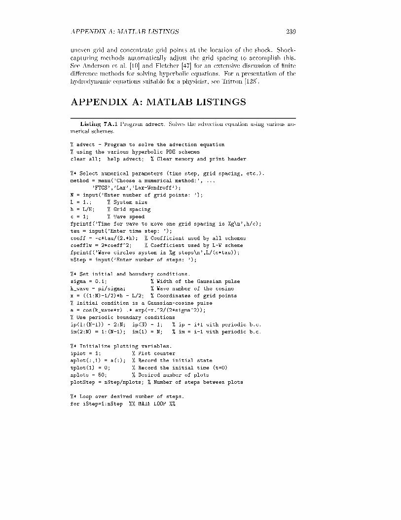
Listing 7A.1 Program advect. Solves the advection equation using various nu-merical schemes.

% advect - Program to solve the advection equation

% using the various hyperbolic PDE schemes

clear all; help advect; % Clear memory and print header

%* Select numerical parameters (time step, grid spacing, etc.).

method = menu('Choose a numerical method:', ...

'FTCS','Lax','Lax-Wendroff');

N = input('Enter number of grid points: ');

L = 1.; % System size

h = L/N; % Grid spacing

c = 1; % Wave speed

fprintf('Time for wave to move one grid spacing is %g\n',h/c);

tau = input('Enter time step: ');

coeff = -c*tau/(2.*h); % Coefficient used by all schemes

coefflw = 2*coeff^2; % Coefficient used by L-W scheme

fprintf('Wave circles system in %g steps\n',L/(c*tau));

nStep = input('Enter number of steps: ');

%* Set initial and boundary conditions.

sigma = 0.1; % Width of the Gaussian pulse

k_wave = pi/sigma; % Wave number of the cosine

x = ((1:N)-1/2)*h - L/2; % Coordinates of grid points

% Initial condition is a Gaussian-cosine pulse

a = cos(k_wave*x) .* exp(-x.^2/(2*sigma^2));

% Use periodic boundary conditions

ip(1:(N-1)) = 2:N; ip(N) = 1; % ip = i+1 with periodic b.c.

im(2:N) = 1:(N-1); im(1) = N; % im = i-1 with periodic b.c.

%* Initialize plotting variables.

iplot = 1; % Plot counter

aplot(:,1) = a(:); % Record the initial state

tplot(1) = 0; % Record the initial time (t=0)

nplots = 50; % Desired number of plots

plotStep = nStep/nplots; % Number of steps between plots

%* Loop over desired number of steps.

for iStep=1:nStep %% MAIN LOOP %%


%* Compute new values of wave amplitude using FTCS,

% Lax or Lax-Wendroff method.

if( method == 1 ) %%% FTCS method %%%

a(1:N) = a(1:N) + coeff*(a(ip)-a(im));

elseif( method == 2 ) %%% Lax method %%%

a(1:N) = .5*(a(ip)+a(im)) + coeff*(a(ip)-a(im));

else %%% Lax-Wendroff method %%%

a(1:N) = a(1:N) + coeff*(a(ip)-a(im)) + ...

coefflw*(a(ip)+a(im)-2*a(1:N));

end

%* Periodically record a(t) for plotting.

if( rem(iStep,plotStep) < 1 ) % Every plot_iter steps record

iplot = iplot+1;

aplot(:,iplot) = a(:); % Record a(i) for ploting

tplot(iplot) = tau*iStep;

fprintf('%g out of %g steps completed\n',iStep,nStep);

end

end

%* Plot the initial and final states.

figure(1); clf; % Clear figure 1 window and bring forward

plot(x,aplot(:,1),'-',x,a,'--'); legend('Initial','Final');

xlabel('x'); ylabel('a(x,t)');

pause(1); % Pause 1 second between plots

%* Plot the wave amplitude versus position and time


mesh(tplot,x,aplot); ylabel('Position'); xlabel('Time');

zlabel('Amplitude');

view([-70 50]); % Better view from this angle

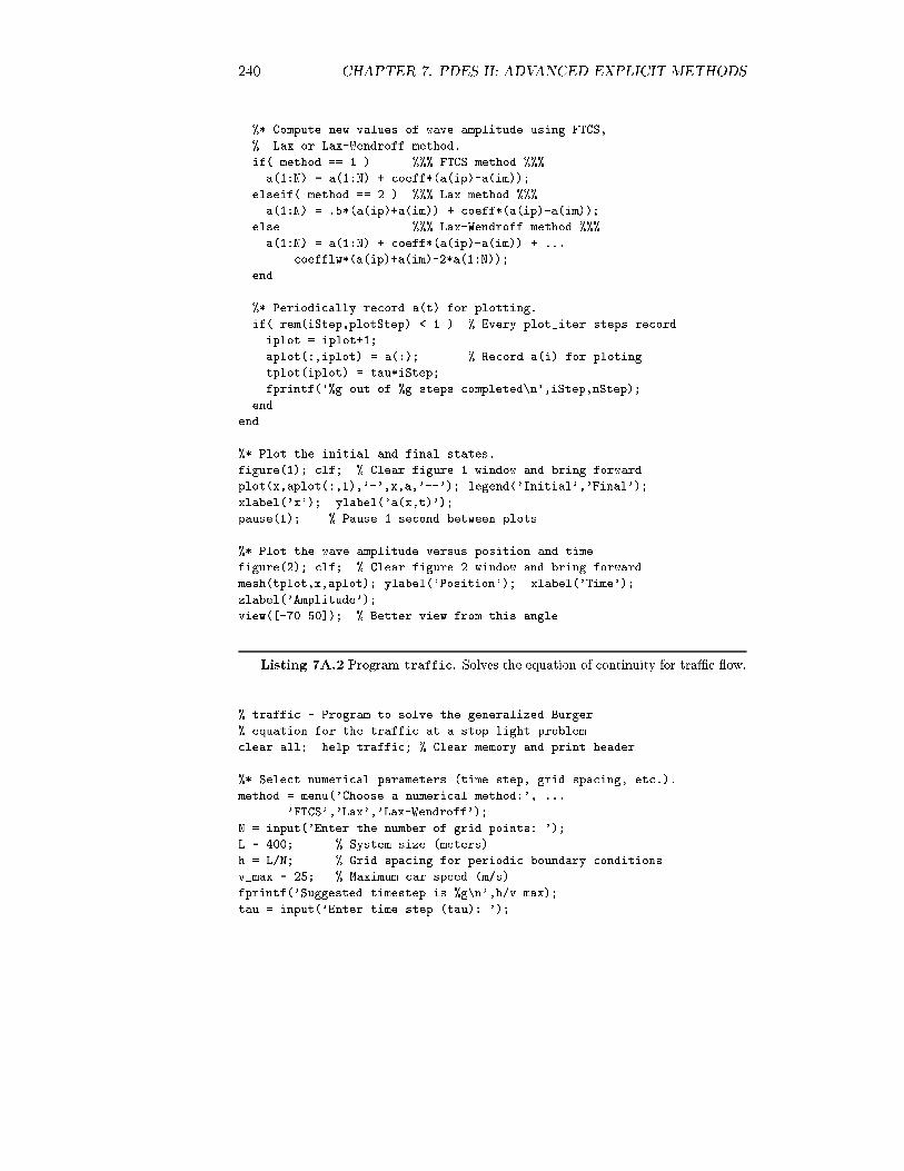
Listing 7A.2 Program traffic. Solves the equation of continuity for traÆc ow.

% traffic - Program to solve the generalized Burger

% equation for the traffic at a stop light problem

clear all; help traffic; % Clear memory and print header

%* Select numerical parameters (time step, grid spacing, etc.).

method = menu('Choose a numerical method:', ...

'FTCS','Lax','Lax-Wendroff');

N = input('Enter the number of grid points: ');

L = 400; % System size (meters)

h = L/N; % Grid spacing for periodic boundary conditions

v_max = 25; % Maximum car speed (m/s)

fprintf('Suggested timestep is %g\n',h/v_max);

tau = input('Enter time step (tau): ');

APPENDIX A: MATLAB LISTINGS 241

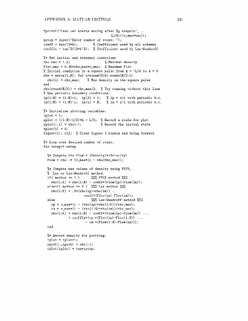
fprintf('Last car starts moving after %g steps\n', ...

(L/4)/(v_max*tau));

nstep = input('Enter number of steps: ');

coeff = tau/(2*h); % Coefficient used by all schemes

coefflw = tau^2/(2*h^2); % Coefficient used by Lax-Wendroff

%* Set initial and boundary conditions

rho_max = 1.0; % Maximum density

Flow_max = 0.25*rho_max*v_max; % Maximum Flow

% Initial condition is a square pulse from x = -L/4 to x = 0

rho = zeros(1,N); for i=round(N/4):round(N/2-1)

rho(i) = rho_max; % Max density in the square pulse

end

rho(round(N/2)) = rho_max/2; % Try running without this line

% Use periodic boundary conditions

ip(1:N) = (1:N)+1; ip(N) = 1; % ip = i+1 with periodic b.c.

im(1:N) = (1:N)-1; im(1) = N; % im = i-1 with periodic b.c.

%* Initialize plotting variables.

iplot = 1;

xplot = ((1:N)-1/2)*h - L/2; % Record x scale for plot

rplot(:,1) = rho(:); % Record the initial state

tplot(1) = 0;


%* Loop over desired number of steps.

for istep=1:nstep

%* Compute the flow = (Density)*(Velocity)

Flow = rho .* (v_max*(1 - rho/rho_max));

%* Compute new values of density using FTCS,

% Lax or Lax-Wendroff method.

if( method == 1 ) %%% FTCS method %%%

rho(1:N) = rho(1:N) - coeff*(Flow(ip)-Flow(im));

elseif( method == 2 ) %%% Lax method %%%

rho(1:N) = .5*(rho(ip)+rho(im)) ...

- coeff*(Flow(ip)-Flow(im));

else %%% Lax-Wendroff method %%%

cp = v_max*(1 - (rho(ip)+rho(1:N))/rho_max);

cm = v_max*(1 - (rho(1:N)+rho(im))/rho_max);

rho(1:N) = rho(1:N) - coeff*(Flow(ip)-Flow(im)) ...

+ coefflw*(cp.*(Flow(ip)-Flow(1:N)) ...

- cm.*(Flow(1:N)-Flow(im)));

end

%* Record density for plotting.

iplot = iplot+1;

rplot(:,iplot) = rho(:);

tplot(iplot) = tau*istep;


%* Display snap-shot of density versus position

plot(xplot,rho,'-',xplot,Flow/Flow_max,'--');

xlabel('x'); ylabel('Density and Flow');

legend('\rho(x,t)','F(x,t)');

axis([-L/2, L/2, -0.1, 1.1]);

drawnow;

end

%* Graph density versus position and time as wire-mesh plot


mesh(tplot,xplot,rplot) xlabel('t'); ylabel('x'); zlabel('\rho');

title('Density versus position and time');

view([100 30]); % Rotate the plot for better view point


%* Graph contours of density versus position and time.


% Use rot90 function to graph t vs x since

% contour(rplot) graphs x vs t.

clevels = 0:(0.1):1; % Contour levels

cs = contour(xplot,tplot,flipud(rot90(rplot)),clevels);

clabel(cs); % Put labels on contour levels

xlabel('x'); ylabel('time'); title('Density contours');

APPENDIX B: C++ LISTINGS

Listing 7B.1 Program advect. Solves the advection equation using various nu-merical schemes.

// advect - Program to solve the advection equation

// using the various hyperbolic PDE schemes

#include "NumMeth.h"

void main() {

//* Select numerical parameters (time step, grid spacing, etc.).

cout << "Choose a numerical method: 1) FTCS, 2) Lax, 3) Lax-Wendroff : ";

int method; cin >> method;

cout << "Enter number of grid points: "; int N; cin >> N;

double L = 1.; // System size

double h = L/N; // Grid spacing

double c = 1; // Wave speed

cout << "Time for wave to move one grid spacing is " << h/c << endl;

cout << "Enter time step: "; double tau; cin >> tau;

double coeff = -c*tau/(2.*h); // Coefficient used by all schemes

APPENDIX B: C++ LISTINGS 243

double coefflw = 2*coeff*coeff; // Coefficient used by L-W scheme

cout << "Wave circles system in " << L/(c*tau) << " steps" << endl;

cout << "Enter number of steps: "; int nStep; cin >> nStep;

//* Set initial and boundary conditions.

const double pi = 3.141592654;

double sigma = 0.1; // Width of the Gaussian pulse

double k_wave = pi/sigma; // Wave number of the cosine

Matrix x(N), a(N), a_new(N);

int i,j;

for( i=1; i<=N; i++ ) {

x(i) = (i-0.5)*h - L/2; // Coordinates of grid points

// Initial condition is a Gaussian-cosine pulse

a(i) = cos(k_wave*x(i)) * exp(-x(i)*x(i)/(2*sigma*sigma));

}

// Use periodic boundary conditions

int *ip, *im; ip = new int [N+1]; im = new int [N+1];

for( i=2; i<N; i++ ) {

ip[i] = i+1; // ip[i] = i+1 with periodic b.c.

im[i] = i-1; // im[i] = i-1 with periodic b.c.

}

ip[1] = 2; ip[N] = 1;

im[1] = N; im[N] = N-1;

//* Initialize plotting variables.

int iplot = 1; // Plot counter

int nplots = 50; // Desired number of plots

double plotStep = ((double)nStep)/nplots;

Matrix aplot(N,nplots+1), tplot(nplots+1);

tplot(1) = 0; // Record the initial time (t=0)

for( i=1; i<=N; i++ )

aplot(i,1) = a(i); // Record the initial state

//* Loop over desired number of steps.

int iStep;

for( iStep=1; iStep<=nStep; iStep++ ) {

//* Compute new values of wave amplitude using FTCS,

// Lax or Lax-Wendroff method.

if( method == 1 ) ////// FTCS method //////

for( i=1; i<=N; i++ )

a_new(i) = a(i) + coeff*( a(ip[i])-a(im[i]) );

else if( method == 2 ) ////// Lax method //////

for( i=1; i<=N; i++ )

a_new(i) = 0.5*( a(ip[i])+a(im[i]) ) +

coeff*( a(ip[i])-a(im[i]) );

else ////// Lax-Wendroff method //////

for( i=1; i<=N; i++ )

a_new(i) = a(i) + coeff*( a(ip[i])-a(im[i]) ) +

coefflw*( a(ip[i])+a(im[i])-2*a(i) );


a = a_new; // Reset with new amplitude values

//* Periodically record a(t) for plotting.

if( fmod((double)iStep,plotStep) < 1 ) {

iplot++;


for( i=1; i<=N; i++ )

aplot(i,iplot) = a(i); // Record a(i) for ploting

cout << iStep << " out of " << nStep << " steps completed" << endl;

}

}

nplots = iplot; // Actual number of plots recorded

//* Print out the plotting variables: x, a, tplot, aplot

ofstream xOut("x.txt"), aOut("a.txt"),

tplotOut("tplot.txt"), aplotOut("aplot.txt");

for( i=1; i<=N; i++ ) {

xOut << x(i) << endl;

aOut << a(i) << endl;

for( j=1; j<nplots; j++ )

aplotOut << aplot(i,j) << ", ";

aplotOut << aplot(i,nplots) << endl;

}

for( i=1; i<=nplots; i++ )

tplotOut << tplot(i) << endl;

delete [] ip, im; // Release allocated memory

}

/***** To plot in MATLAB; use the script below ********************

%* Plot the initial and final states.

load x.txt; load a.txt; load tplot.txt; load aplot.txt;


plot(x,aplot(:,1),'-',x,a,'--'); legend('Initial','Final');

xlabel('x'); ylabel('a(x,t)');


%* Plot the wave amplitude versus position and time


mesh(tplot,x,aplot); ylabel('Position'); xlabel('Time');

zlabel('Amplitude');

view([-70 50]); % Better view from this angle

******************************************************************/

Listing 7B.2 Program traffic. Solves the equation of continuity for traÆc ow.

// traffic - Program to solve the generalized Burger

// equation for the traffic at a stop light problem

#include "NumMeth.h"


void main() {

//* Select numerical parameters (time step, grid spacing, etc.).

cout << "Choose a numerical method: 1) FTCS, 2) Lax, 3) Lax-Wendroff : ";

int method; cin >> method;

cout << "Enter the number of grid points: "; int N; cin >> N;

double L = 400; // System size (meters)

double h = L/N; // Grid spacing for periodic boundary conditions

double v_max = 25; // Maximum car speed (m/s)

cout << "Suggested timestep is " << h/v_max << endl;

cout << "Enter time step (tau): "; double tau; cin >> tau;

cout << "Last car starts moving after "

<< (L/4)/(v_max*tau) << " steps" << endl;

cout << "Enter number of steps: "; int nStep; cin >> nStep;

double coeff = tau/(2*h); // Coefficient used by all schemes

double coefflw = tau*tau/(2*h*h); // Coefficient used by Lax-Wendroff

double cp, cm; // Variables used by Lax-Wendroff

//* Set initial and boundary conditions

double rho_max = 1.0; // Maximum density

double Flow_max = 0.25*rho_max*v_max; // Maximum Flow

// Initial condition is a square pulse from x = -L/4 to x = 0

Matrix rho(N), rho_new(N);

int i,j, iBack = N/4, iFront = N/2 - 1;

for( i=1; i<=N; i++ )

if( iBack <= i && i <= iFront ) rho(i) = rho_max;

else rho(i) = 0.0;

rho(iFront+1) = rho_max/2; // Try running without this line

// Use periodic boundary conditions

int *ip, *im; ip = new int [N+1]; im = new int [N+1];

for( i=2; i<N; i++ ) {

ip[i] = i+1; // ip[i] = i+1 with periodic b.c.

im[i] = i-1; // im[i] = i-1 with periodic b.c.

}

ip[1] = 2; ip[N] = 1;

im[1] = N; im[N] = N-1;

//* Initialize plotting variables.

int iplot = 1;

Matrix tplot(nStep+1), xplot(N), rplot(N,nStep+1);

tplot(1) = 0.0; // Record initial time

for( i=1; i<=N; i++ ) {

xplot(i) = (i - 0.5)*h - L/2; // Record x scale for plot

rplot(i,1) = rho(i); // Record the initial state

}

//* Loop over desired number of steps.

Matrix Flow(N);

int iStep;


for( iStep=1; iStep<=nStep; iStep++ ) {

//* Compute the flow = (Density)*(Velocity)

for( i=1; i<=N; i++ )

Flow(i) = rho(i) * (v_max*(1.0 - rho(i)/rho_max));

//* Compute new values of density using FTCS,

// Lax or Lax-Wendroff method.

if( method == 1 ) ////// FTCS method //////

for( i=1; i<=N; i++ )

rho_new(i) = rho(i) - coeff*(Flow(ip[i])-Flow(im[i]));

else if( method == 2 ) ////// Lax method //////

for( i=1; i<=N; i++ )

rho_new(i) = 0.5*(rho(ip[i])+rho(im[i]))

- coeff*(Flow(ip[i])-Flow(im[i]));

else ////// Lax-Wendroff method //////

for( i=1; i<=N; i++ ) {

cp = v_max*(1 - (rho(ip[i])+rho(i))/rho_max);

cm = v_max*(1 - (rho(i)+rho(im[i]))/rho_max);

rho_new(i) = rho(i) - coeff*(Flow(ip[i])-Flow(im[i]))

+ coefflw*(cp*(Flow(ip[i])-Flow(i))

- cm*(Flow(i)-Flow(im[i])));

}

// Reset with new density values

rho = rho_new;

//* Record density for plotting.

cout << "Finished " << iStep << " of " << nStep << " steps" << endl;

iplot++;


for( i=1; i<=N; i++ )

rplot(i,iplot) = rho(i);

}

int nplots = iplot; // Number of plots recorded

//* Print out the plotting variables: tplot, xplot, rplot

ofstream tplotOut("tplot.txt"), xplotOut("xplot.txt"),

rplotOut("rplot.txt");

for( i=1; i<=nplots; i++ )

tplotOut << tplot(i) << endl;

for( i=1; i<=N; i++ ) {

xplotOut << xplot(i) << endl;

for( j=1; j<nplots; j++ )

rplotOut << rplot(i,j) << ", ";

rplotOut << rplot(i,nplots) << endl;

}

delete [] ip, im;

}


/***** To plot in MATLAB; use the script below ********************

load tplot.txt; load xplot.txt; load rplot.txt;

%* Graph density versus position and time as wire-mesh plot


mesh(tplot,xplot,rplot) xlabel('t'); ylabel('x'); zlabel('\rho');

title('Density versus position and time');

view([100 30]); % Rotate the plot for better view point


%* Graph contours of density versus position and time.


% Use rot90 function to graph t vs x since

% contour(rplot) graphs x vs t.

clevels = 0:(0.1):1; % Contour levels

cs = contour(xplot,tplot,flipud(rot90(rplot)),clevels);

clabel(cs); % Put labels on contour levels

xlabel('x'); ylabel('time'); title('Density contours');

******************************************************************/

Documents

Library of Congress Cataloging-in-Publication Data · Garcia San Jose State University Pren tice Hall, Upp er Saddle Riv er, New Jersey 07458. Library of Congress Cataloging-in-Publication