An accompaniment to a course on interest rate

modeling: with discussion of Black-76, Vasicek

and HJM models and a gentle introduction to the

multivariate LIBOR Market Model

Vasily Nekrasov∗

http://www.yetanotherquant.de

July 10, 2013

Abstract

The goal of this paper is to help the motivated students with theircourse on interest rate modeling and/or to help them to learn the LIBORmodel by themselves. It implies the reader knows what forward rates,caps, and swap[tion]s are and has some knowledge of the quantitative fi-nance: at least Ito Calculus, Black-Scholes-[Merton] Formula, Girsanov’sTheorem (in one dimension is enough) and the risk-neutral pricing. Thisstuff is usually taught in the first course on continuous financial modelingand is relatively easy. The interest rate modeling is much more compli-cated. Still those, who carefully read the wonderful Steven Shreve’s bookcan learn the short-rate models, change of numeraire and Heath-Jarrow-Morton framework. But not the multivariate LIBOR Model (though thereis a short section on the one factor LIBOR Model and its relation to theHJM). However, the Bond/IR market is essentially multivariate and theLIBOR Model can be introduced independently. But I could not find anytutorial, which would suit me. So I decided to write my own. It concernstheory only and not the calibration and computational aspects, which arethe issues for the future papers.

1 Typical problems of a quant student

If you read this paper you are probably attending an [advanced] course oninterest-rate modeling. If so, you likely know some short rate models and maybethe HJM framework. Though formally not necessary for studying of the LIBORModel, it is still very helpful to be aware of this stuff. That’s why if you are not, I

∗Many thanks to Dmitri Semenchenko, Dr. Frank Wittemann, Dr. Michael Busch, Dr.Michael Meyer, Dr. Thomas Mazzoni.

1

do recommend to read the respective chapters of Shreve’s book first. Historicaldevelopment was Black-76 → Short rate models → HJM → LIBOR MarketModel → (LIBOR with jumps and stochastic volatility). So starting directlyfrom the LIBOR would mean ignoring the historical roots. So we discuss theearlier models too trying to enlighten some principle ideas, which are frequentlymisunderstood by students.

1.1 The Black formula (Black-76)

The Black-Scholes-[Merton] formula was a breakthrough and still remains themain formula in quantitative finance. Black-76 is its modification for the com-modity(!) market though it is far more frequently used to price the interest ratederivatives. Surprisingly, this formula often lacks attention in the lectures. Forexample, if the lecture notes are based on Brigo and Mercurio, it is introducedwithout derivation (and even motivation) and if they are based on Shreve, itmight be ignored at all since Shreve derives it from LIBOR Model, which comesat the very end of the paragraph on the term structure models. We, in turn, willlearn it thoroughly since the motivation behind the LIBOR is its consistencewith Black-76 [for caplets].

In 1976 Fischer Black wrote his seminal “Pricing of commodity contracts”.His assumptions were that the short rates are constant, the futures prices arelognormally distributed with known variance rate σ2 and the expected changein futures prices is zero. Once again, the extension was intended for commoditymarket: Black, himself, did write about farmers and harvests but did not writeanything about options on bonds, caps and swaptions.

But the market readily adopted his approach ignoring that e.g. bond pricesand forward rates cannot be simultaneously lognormal, let alone that the as-sumption of the constant short rate can do for the grain market but is clearlyabsurd for the bond market. But in the 70th there were few models and if onehas only a hammer at hand, everything around seems to be the nails. So themarket felt fine using the Black-76 long before it was rigorously justified withLIBOR Model. Finally, as Black himself wrote in his another famous paper1:“In the end, a theory is accepted not because it is confirmed by conventionalempirical tests, but because researches persuade one another that the theory iscorrect and relevant”.

Black used the delta hedging to derive his formula (recall that by his timethe risk neutral pricing was not yet discovered, so the delta hedging was an onlytool to price options from no arbitrage assumption). He also appealed to theCAPM (Capital Asset Pricing Model) to motivate his assumptions empirically,stating that “if the covariance of the change in the futures price with the returnon the market portfolio is zero, then the expected change in the futures price will

1Fischer Black, “Noise”. The Journal of Finance, Volume 41, Issue 3 · July 1986

2

be zero” and then recalling an empirical study2 confirming that this is [nearly]the case for the wheat, corn and soybean futures.Now let us quickly discuss what forward and futures contracts are.

Definition 1.1. A forward on an asset X is a contract at time t to sell X atfuture time T (maturity date) at the fixed price K (strike).

Example 1.2. Which strike makes the present value of the forward equal tozero at time t if the interest rate r is constant? (We denote such strike withForX(t, T ) and call it the fair price).

At time t you have no money. The price of the zero T-Bond is P (t, T ) =e−r(T−t). Borrow X(t) [at rate r] and buy one unit of X . At time T you have

to pay back X(t)P (t,T ) and can sell X for X(T ) where X(T ) is the spot price of X

at time T . So from no arbitrage

ForX(t, T )

⋆︷︸︸︷=

X(t)

P (t, T )

†︷︸︸︷= er(T−t)X(t) (1)

The ⋆ in 1 holds even if the interest rate is not constant, all we need is a tradableT-Bond at time t. But for the † a constant interest rate is needed.Forwards are the OTC contracts. Note that a forward, unlike an option, isobligatory for both counterparties.

There is a credit risk since one side can go bankrupt before T . Moreover,the contract must specify in details the quality and quantity of X by delivery.Futures on X solve both problems. Futures are traded on a [commodity] ex-change and are standardized by the exchange. One can loosely consider thefutures as forwards, whose fair prices are reset every day. Denote FutX(t, T )the futures price on X at time t with delivery T . Clearly FutX(T, T ) = X(T ).In order to enter the futures contract one does not need to pay FutX(t, T ),indeed it costs nothing to enter the futures contract (fair price). One still paysthe safety margin but to the exchange, not to the counterparty. This is in noway the price of the contract but just a collateral to eliminate the default risk.If, for example X(t1, T ) = 100, X(t2, T ) = 110 and one went long in the futurescontract at time t1, his gain at time t2 is 10, which is immedeately paid bythe counterparty. If the counterparty cannot pay, the exchange pays from thesafety margin and the contract gets closed. On maturity date T one pays theX(t1, T ) = 100 and receives a commodity. The sum of daily payments generatedby this futures contract is

(X(t2, T )−X(t1, T ))+(X(t3, T )−X(t2, T ))+ . . .+(X(ti, T )−X(ti−1, T ))+ . . .

+ (X(T, T )−X(tn−1, T ) = X(T, T )−X(t1, T ) = X(T )−X(t1, T ) (2)

2Dusak K., 1973 Futures trading and investor returns: An investigation of commoditymarket risk premiums, Journal of Political Economy 81, Nov./Dec., 1387-1406

3

Stop for a while and make sure you do understand the idea of a futures contract(check the Hull’s book if you don’t). Otherwise you will not understand 5.Note that normally there is a daily accrued interest on the account to(from)which X(ti, T )−X(ti−1, T ) flows on the i-th day, so 2 is not a profit(loss) of afutures contract unless the interest rate is equal to zero.

Now we turn back to the Black-76 formula. For simplicity denote F (t) =FutX(t, T ) (we can do so since T is arbitrary but fixed). Under the Black’sassumptions(lognormality and expected zero change of the futures prices) wecan write the dynamics of F (t) as

dF (t) = σF (t)dW (t) (3)

At time t we consider a call option with a strike K and the maturity T on thefutures contract with delivery at time S, t < T < S. For the price of this calloption we write C(t, F (t), r, T, S,K) = C(t, F ) since r, T , S and K are arbitrarybut fixed. By Ito Formula we obtain

dC(t, F (t)) = Ctdt+ CFdF (t) +1

2CFFd

2F (t)

= Ctdt+ σCFF (t)dW (t) +1

2CFFσ

2F 2(t)dt (4)

We can eliminate the random factor σCFF (t)dW (t) from 4 if we go short inCF futures contract at time t. Following Black, we denote the initial value ofthe futures contract with u(t). It follows that u(t) = 0 since it costs nothing toenter the contract with futures price F (t). But obviously as time goes to t+ dt,a futures contract generates a cashflow F (t+ dt)− F (t), i.e.

du(t) = dF (t) = σF (t)dW (t) (5)

So a portfolio C(t, F ) − u(t)CF , i.e. with a call long and CF futures short isriskless (no dW factor) and evolves according to

d (C(t, F )− u(t)CF ) = Ctdt+1

2CFFσ

2F 2(t)dt = r (C(t, F )− u(t)CF ) (6)

The right-hand part is due to no-arbitrage: every riskless portfolio Π must growaccording to dΠ = rΠdt. But u(t) = 0 and finally we get

Ctdt+1

2CFFσ

2F 2(t)dt = rC(t, F ) (7)

The solution of this equation is the famous Black-76 Formula

C(t, F (t), r, T, S,K) = F (t)e−r(T−t)N (d1)−Ke−r(T−t)N (d2) (8)

where

d1 =1

σ√T

[

ln

(F (t)

K

)

+1

2σ2T

]

4

d2 = d1 − σ√T =

1

σ√T

[

ln

(F (t)

K

)

− 1

2σ2T

]

It is a useful exercise to compare the derivation of Black-76 with BS-Formula3.

Note that there is a dependence on S (futures delivery date) only in termF (t) := FutX(t, S) (price at time t of the futures with delivery date S). Itshould be clear, since what matters is the difference F (T ) − K. An optionholder may even not enter the futures contract at T but just take a cash settle-ment [F (T )−K]+ (recall, it costs nothing to enter the futures contract).In particular, F (S) := FutX(S, S) = X(S) so setting S = T in 8 we obtain theprice of the option on commodity itself (and not on commodity futures).

Black also derived from 8 the price of the forward contract with arbitrarystrikeK, using the terminal condition v(X,T,K, T ) = X(T )−K, where v(X, t,K, T )is the value at time t of the forward contract on asset X with the strike K anddelivery date T . Black obtained

v(X, t,K, T ) = (FutX(t, T )−K)er(T−t) (9)

Setting K = ForX(t, T ) yields v(X, t,K, T ) = 0 and thus

ForX(t, T ) = FutX(t, T ) (10)

so can one use the Black-76 for options on forward as well?!

In fact 10 holds only if the interest rate is deterministic!You may read about the forward-future spread (and the definition of futuresprice as an expectation w.r.t. the martingale measure) in Shreve’s book. Butfor the rest of this paper it is not necessary since even if 10 would always hold,the assumption of a constant interest rate and lognormal forward rates is itselfclearly absurd.Does it invalidate the Black Formula for caplets? Obviously not necessarily, itonly shows that one cannot derive it from current assumptions. So in the LIBORModel the assumptions are slightly modified: the forwards are still lognormalbut each under its Ti-forward measure. By change of measure(and numeraire)we make the interest rate irrelevant. So if you are interested only in LIBORmodel jump to 1.4. But if you would like to understand why the LIBOR modelis good (besides that it makes Black-76 valid) and probably find answers tosome puzzles of short-rate models then read the whole stuff.

3http://en.wikipedia.org/wiki/Black-Scholes (Section The BlackScholes equation).

5

1.2 Short-rate Models and the martingale measure

Short rate is an instantaneous time dependent interest rate rt so that the bankaccount (with initial investment of 1e) grows according to

B(t) = exp

t∫

0

r(s)ds

(11)

Respectively, by the risk neutral pricing, the price of a T-Bond at time T is

P (t, T ) = EQ

[Bt

BT

∣∣Ft

]

= EQ

exp

−T∫

t

r(s)ds

∣∣∣Ft

(12)

where Q is the martingale measure. rt can be (and really is) stochastic but attime t we know how our bank account will change in an infinitesimal timespan.On the other hand the respective change of a T-Bond price is unpredictablesince it depends not only on rt but also on future short rates up to T. We canrewrite 11 as dB(t) = rBdt, so B(t) is differentiable and thus “less random”than a T-Bond. We can define a discounted T-Bond by

Z(t, T ) = D(t)P (t, T ) = P (t, T )/B(t) (13)

The dynamics of Z(t, T ) must be a martingale under Q. But the dynamics ofrt need not since bonds are tradable and rt is not.The first short rate model is due to Vasicek (1977)4

dr(t) = (a− brt)dt+ σdWt (14)

In modern books the model is often introduced directly under the risk neu-tral measure Q (so that in 14 actually stays dWQ

t ) and a student with a stockprice modeling background gets puzzled: in stock market we observed a stock(a tradable asset) under the real measure than killed the drift to make it mar-tingale. As you [should] remember, there is no arbitrage iff there is a martingalemeasure (so that the discounted prices of all tradable assets are martingales).And the market is complete iff the martingale measure is unique. But how toproceed with rt, which is untradable and thus need not to be a martingale?!Moreover, it is unobservable even under the real measure5). Finally, does Qexist at all and if it does, is it unique?!

We will follow the original Vasicek’s paper (which is far more often cited than

4Indeed, Vasicek started with much more general settings and considered 14 just as aspecial case. Merton’s Model (1973) was actually published earlier but still Vasicek is somehowconsidered as the first, well, at least in the most of textbooks.

5Garatek et al (p. xiii) say that the overnight rate is a good proxy for the short rate butFilipovic (p.10) argues it is not “because the motives and needs driving overnight borrowersare very different from those of borrowers who want money for a month or more”.

6

read)6 and see how Vasicek have introduced the market price of risk. There isno martingale measures in his paper since the risk neutral approach was intro-duced several years later by Harrision, Kreps and Pliska. However, as soon aswe have the market price of risk λt we can introduce the risk neutral measureby Girsanov’s theorem and turn back to ”more modern” risk neutral approach.

In a short-rate model the bond price depends on t, rt and T so we writeP (t, T ) = f(t, rt, T )

7, whereas T is arbitrary but fixed. By Ito formula thedynamics of the bond price is

df = f(t)dt+ f(r)drt+1

2f(rr)d

2rt

(14)︷︸︸︷= (f(t)+[a− brt]f(r)+

σ2

2f(rr))dt+σf(r)dWt

(15)which we can rewrite as

df(t, rt, T ) = f(t, rt, T ) [µ(t, rt, T )dt+ ν(t, rt, T )dWt] (16)

where

µ(t, rt, T ) =f(t) + [a− brt]f(r) +

σ2

2 f(rr)

f(t, rt, T )

ν(t, rt, T ) =σf(r)

f(t, rt, T )

The formula 16 resembles us the old good lognormal dynamics of a stockprice, where µ(t, rt, T ) and ν(t, rt, T ) are respectively the drift and the volatil-ity coefficients. (A reader, who studied the multivariate stock market modelmight anticipate that we are going to talk about the market price of risk[µ(t, rt, T )− rt]/ν(t, rt, T ))

Now consider an investor who at time t issues an amount U1 of a bond withmaturity date T1 and simultaneously buys an amount U2 of a bond maturingat time T2. The total value of this portfolio is U = U2 − U1 and it evolvesaccording to

dU = [U2µ(t, rt, T2)−U1µ(t, rt, T1)]dt+[U2ν(t, rt, T2)−U1ν(t, rt, T1)]dWt (17)

We can eliminate the stochastic risk factor in 17 choosing

U1 = Uν(t, rt, T2)

ν(t, rt, T1)− ν(t, rt, T2)U2 = U + U1 = U

ν(t, rt, T1)

ν(t, rt, T1)− ν(t, rt, T2)

Such portfolio is riskless (there is only the drift term [U2µ(t, rt, T2)−U1µ(t, rt, T1)]dt) and thus by no arbitrage assumption (cp. with 6)

U[µ(t, rt, T2)ν(t, rt, T1)− µ(t, rt, T1)ν(t, rt, T2)]

ν(t, rt, T1)− ν(t, rt, T2)dt = rtUdt (18)

6http://www.wilmott.com/messageview.cfm?catid=4&threadid=859487This holds only if rt is a Markov process (in our case it is), otherwise P (t, T ) may addi-

tionally depend on rs for all s ∈ [0, t]

7

or equivalentlyµ(t, rt, T2)− rt

ν(t, rt, T2)=

µ(t, rt, T1)− rtν(t, rt, T1)

=: λt (19)

where λt can be interpreted as the market price of risk. Note that it must bethe same for all bonds and thus does note depend on bond maturity (but ofcourse may depend on t and rt). But what risk do we actually mean? Well, aswe stated before, the bank account is ”less random” than a bond, so we expectan excess return on a bond. The longer is the maturity of a bond the larger isits volatily ν(t, rt, T ) and respectively its expected excess return µ(t, rt, T )− rtbut their ratio does not varies with T .Writing 19 as

µ(t, rt, T )− rt = λtν(t, rt, T ) (20)

and substituting for µ(t, rt, T ) and ν(t, rt, T ) from 16 we get the term structureequation

f(t) + [a− λtσ − brt]f(r) +σ2

2f(rr) − rtf = 0 (21)

with the terminal condition

f(T, rT , T ) = 1

The term structure equation has a solution8 so the model at least does not con-tradict the no arbitrage assumption which we engaged before. Respectively, amartingale measure exists.

On the other hand the Girsanov’s theorem tells us that dWQt = θtdt + dWt

for some process θt and it only remains to show that indeed θt = λt . Rewriting14 under Q we obtain

dr(t) = (a− brt − σθt)dt+ σdWQt (22)

Writing as before f = f(t, rt, T ) for the price of a T-Bond at time t we obtainby the Ito product rule d[Dtf ] = −rtDtf +Dtdf so

d[Dtf ] = −rtDtfdt+Dt

[

f(t) + f(r)(a− brt − σθt) +σ

2f(rr)

]

dt+ σf(r)DtdWQt

(23)Since the discounted price is a martingale the drift (dt-term) must be zero.Comparing 23 with 21 we conclude that θt = λt and assign κt := a− λtσ

So we showed why and how we can model directly under the risk neutral mea-sure. However, the model does not imply any restrictions from which followsthat λt must be unique. Within the model is just required that λt must be thesame for all bonds but we can arbitrarily choose it. For different λt we will getdifferent bond prices, all of them arbitrage free. But having only model at hand

8see Shreve’s book how to use the Ansatz f(t, rt, T ) = exp(−rtC(t, T )−A(t, T ))

8

we cannot choose the “right” λt. Thus the model as such is not complete.What you need to understand now is that the market players, not a model,define the martingale measure. And if the market players have the same infor-mation and the same risk preference the market will be complete. Of courseit is not so in practice but we like assuming it because if we do, the pricing ofevery bounded contingent claim is, in principle, possible. So we assume thatthe market is complete and moreover, that the market price of risk is constant,i.e. λt ≡ λ. Next we realize that bonds were traded long before the quantita-tive models appeared :). Since the term structure equation gives us the [closedform] solution for the bond price, we can calibrate the model and choose theparameters (κ, b, σ) to fit the bond prices (and usually some liquid derivativeslike caps and swaptions) as good as possible. Then we can use the model toprice any other derivatives. Note that we can find κ but not λ directly, sincethe dynamics of the short rate is unobservable. This is the difference with e.g.the Black-Scholes model, in which we can [at least theoretically] find the driftµ and thus the market price of risk µ−r

σ.

Note that the assumption of the constant parameters is too restrictive, so theVasicek model generally cannot perfectly fit the current term structure. It isthe difference between the equilibrium and the arbitrage free models. The for-mer usually assume some equilibrium in demand and supply(mean reversion isa kind of such equilibrium) and generate the term structure as an output. Thelatter can be perfectly matched to the current term structure (but not necessar-ily to the current caps and swaptions prices). Vasicek, CIR are the equilibriummodels and Ho Lee, Hull White, Black Karasinski, G2 are the arbitrage freemodels. Such fitting is achieved via a time dependent parameter, e.g. in HullWhite Model κ is time dependent:

dr(t) = (κ(t)− brt)dt+ σdWQt (24)

Recall that in the Vasicek Model κ is constant.

1.3 Some aspects of Heath-Jarrow-Morton

The [one factor] HJM Model is well discussed in Shreve’s book and it wouldhave made little sense to blueprint it here. Instead, we discuss some aspectswhich may help you to go on with Shreve.

1. Motivation. HJM models not the short rate but rather the whole forwardcurve. The model is complete and the drift under the risk neutral measure turnsout to be fully determined by the volatility. See Shreve for more details.

2. Instantaneous forward rate. If the interest is continiously compound, theforward rate f(t, T, T + δ) is defined from

P (t, T ) = eδf(t,T,T+δ)P (t, T + δ) ⇔ f(t, T, T + δ) =1

δln

(P (t, T )

P (t, T + δ)

)

9

Letting δ → 0 we obtain

limδ→0

ln(P (t, T ))− ln(P (t, T + δ))

δ= −∂ln(P (t, T ))

∂T=: f(t, T ) (25)

Setting T = t we get the instantaneous short rate R(t) = f(t, t). Note that theinstantaneous forward rate is unobservable too.

3. It turns out that the affine short rate models, i.e. those for which P (t, rt, T ) =exp(−rtC(t, T )−A(t, T )) can be embedded in HJM via the drift term condition.See Shreve for more details.

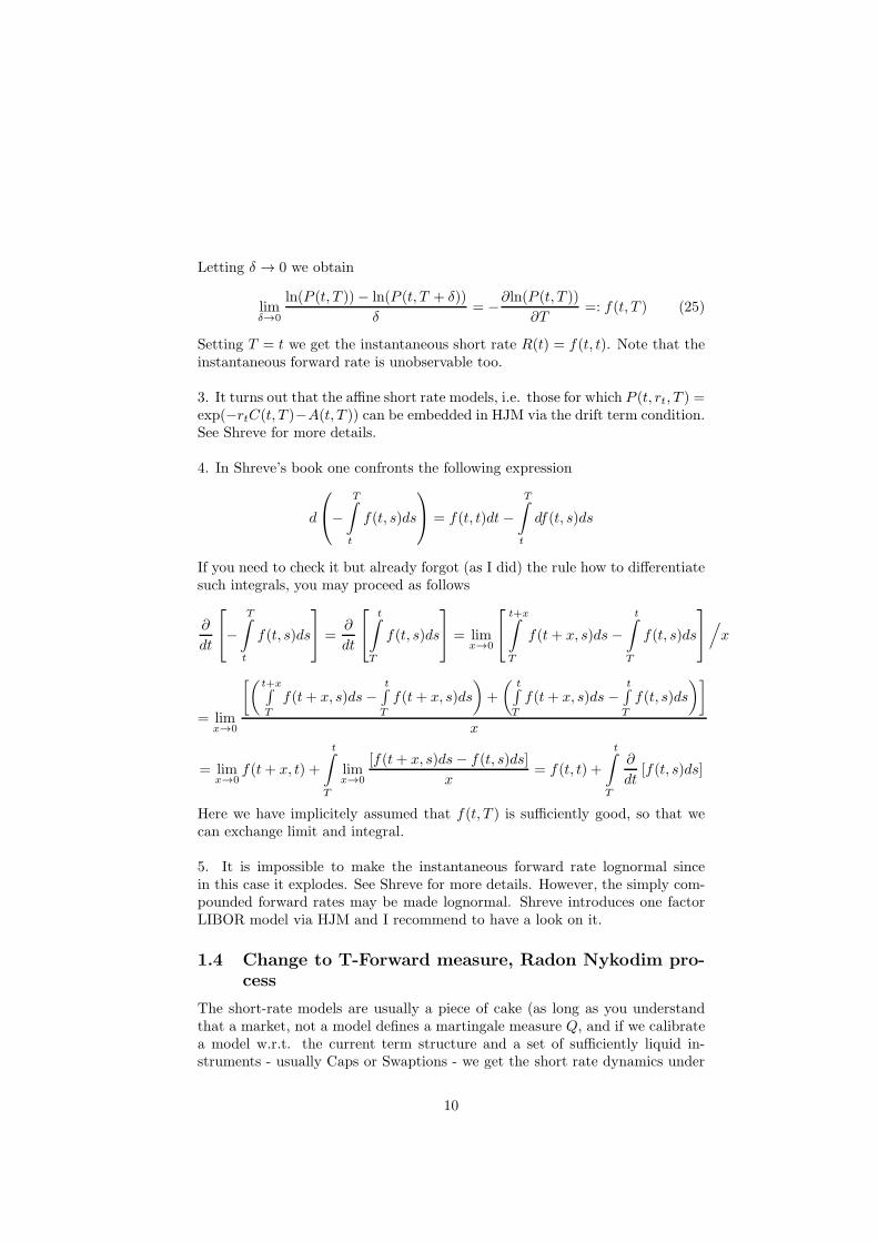
4. In Shreve’s book one confronts the following expression

d

−T∫

t

f(t, s)ds

= f(t, t)dt−T∫

t

df(t, s)ds

If you need to check it but already forgot (as I did) the rule how to differentiatesuch integrals, you may proceed as follows

∂

dt

−T∫

t

f(t, s)ds

=∂

dt

t∫

T

f(t, s)ds

= limx→0

t+x∫

T

f(t+ x, s)ds−t∫

T

f(t, s)ds

/

x

= limx→0

[(t+x∫

T

f(t+ x, s)ds−t∫

T

f(t+ x, s)ds

)

+

(t∫

T

f(t+ x, s)ds −t∫

T

f(t, s)ds

)]

x

= limx→0

f(t+ x, t) +

t∫

T

limx→0

[f(t+ x, s)ds− f(t, s)ds]

x= f(t, t) +

t∫

T

∂

dt[f(t, s)ds]

Here we have implicitely assumed that f(t, T ) is sufficiently good, so that wecan exchange limit and integral.

5. It is impossible to make the instantaneous forward rate lognormal sincein this case it explodes. See Shreve for more details. However, the simply com-pounded forward rates may be made lognormal. Shreve introduces one factorLIBOR model via HJM and I recommend to have a look on it.

1.4 Change to T-Forward measure, Radon Nykodim pro-cess

The short-rate models are usually a piece of cake (as long as you understandthat a market, not a model defines a martingale measure Q, and if we calibratea model w.r.t. the current term structure and a set of sufficiently liquid in-struments - usually Caps or Swaptions - we get the short rate dynamics under

10

Q). The HJM is usually managable too, at least Shreve makes it so. But it isthe change of numeraire / T-Forward measures what makes troubles. Often aT-Forward measure QT is introduced as

dQT :=1

P (0, T )BT

dQ (26)

which is actually

dQT :=P (T, T )

P (0, T )BT

dQ (27)

It is easy to prove that it is indeed a probability measure. (Can you do it? If not,don’t worry, we will do it later). dQT /dQ is a Radon-Nikodym derivative fromt = 0 and with T in mind. But we need a Radon-Nikodym (a.k.a. likelihood)process for all t ∈ [0, T ]. It is

ηt :=P (t, T )

P (0, T )Bt

(28)

but unfortenately it often appears just like rabbit out of the hat. Soon we willconsider its derivation in detail but so far just note the term P (t, T ) in thenumerator. So you can guess for what I state that 26 is actually 27.As soon as we have ηt we can find at time t the price π(XT ) of a contingentclaim XT using the T-Forward measure since

EQT [XT |Ft] =1

ηtEQ [XT ηT |Ft] =

B(t)P (0, T )

P (t, T )EQ

[

XT

P (T, T )

B(T )P (0, T )

∣∣∣Ft

]

=1

P (t, T )EQ

[

XT

B(t)

B(T )

∣∣∣Ft

]

=1

P (t, T )π(XT ) (29)

Under Q there is a quotient of XT and BT whereas under QT we have onlyXT . So the formula 29 is useful when XT and BT are dependent, which is thecase for the interest rate derivatives. However, this formula is just an elegantbut useless theoretical construction until we specify the dynamics of X(t) underQT . To do this we need to understand the change of numeraire for which, inturn, we need the

2 Multivariate Girsanov’s Theorem and Cholesky

decomposition

2.1 Preliminaries

Before we state the multivariate Girsanov’s theorem, we will explain what ηt isin the discrete case (on a binary tree) and then prove two useful lemmas for ηtin continuous time.So let us recall the change from the objective measure P to the martingale

11

measure Q on a binary tree. Q is not a T-Forward measure (Q is called the spotmeasure) but for a discussion of the Radon-Nykodim process this is irrelevant.

(A):1

(B): 1−q1−p

(C): qp

(D): (1−q)2

(1−p)2

(E): q(1−q)p(1−p)

(F): q2

p2

(G): q3

p3

(H): q2(1−q)

p2(1−p)

(I): q(1−q)2

p(1−p)2

(J): (1−q)3

(1−p)3

(1 − p)

(1 − q)

qp

I noted before that the T-Forward measure is defined from t = 0 with T inmind. In our case T corresponds to the last four nodes: (G), (H), (I) and (J).Though Q is not a T-Forward measure, the Radon Nykodim derivative (in thesense of the classical Real Analysis) is still defined from t = 0 and with T inmind. (Or in our case it is better to say “from (A) with (G), (H), (I), (J) inmind”). Namely, for a measurable space (Ω,F) and two absolutely continuousmeasures Q and P on (Ω,F) (i.e which agree about the measure-zero sets of Ω)there is a unique9 function f , called the Radon Nykodim derivative, such that

Q(A) =

∫

A

f(ω)dP (ω)

⋆︷︸︸︷= EP [f(ω)1A] = EP [f(ω)1A|F0] ∀A ∈ F (30)

The ⋆ in 30 is valid if P is a probability measure (in our case it is by def-inition). The question is in which case is Q a probability measure as well?An obvious necessary and sufficient condition is the nonnegativity of f and∫

Ωf(w)dP (ω) = 1 must hold true. Indeed, Q is a measure (i.e. Q(∅) = 0 and

Q is σ-additive) by the Radon Nykodim theorem. And since Q(Ω) = 1 it is aprobability measure10.

9Upto a set of measure zero w.r.t. P10Now I am sure you can prove that QT defined in 26 is a probability measure.

12

In our case the Radon Nykodim derivative is defined according to Table 1:

Table 1: Radon Nykodim derivative from (A) to (G), (H), (I), (J) in mindω (G) (H) (I) (J)

f(ω) q3

p3

q2(1−q)p2(1−p)

q(1−q)2

p(1−p)2(1−q)3

(1−p)3

Because the measures are discrete, an integral in 30 becomes just a sum and

Q(Ω) =

∫

Ω

f(ω)dP (ω) =q3

p3p3 +

q2(1− q)

p2(1− p)3p2(1− p)

+q(1− q)2

p(1− p)23p(1− p)2 +

(1− q)3

(1 − p)3(1− p)3 = 1

Considering ⋆ in 30 more generally, we want to express the expectationsw.r.t. Q as the expectations w.r.t. P . For any random variable X ∈ F it isactually

EQ [X ] =

∫

Ω

XdQ(ω) =

∫

Ω

Xf(ω)dP (ω) = EP [f(ω)X ] (31)

But we are interested not only in the single Radon Nykodim derivative. Ratherwe want to define the Radon Nykodim process ηt so that (G), (H), (I), (J) inmind stays but now we are looking from any node, not only from (A). It is justlike replacing P (T, T ) and BT in 27 with P (t, T ) and Bt in 28. We can definethe Radon Nykodim derivative e.g. from (C) to (G), (H), (I), (J) in mind(Table 2). Note that it is impossible to move in (J) from (C), so the respective

Table 2: Radon Nykodim derivative from (C) to (G), (H), (I), (J) in mindω (G) (H) (I) (J)

f(ω) q2

p2

q(1−q)p(1−p)

(1−q)2

(1−p)2 0

probability is set to zero.

However, such approach is indeed not what we need. What do we need toprice derivatives? Just to take expectation w.r.t. the martingale measure andsometimes express this expectation via expectation w.r.t. the real and T-forwardmeasures. Now recall 31! So we do not need the Radon Nykodim process asa function, we only need it in the sense of expectation, however, conditionalexpectation, given a σ-algebra Ft.So we define the Radon Nykodim process as

ηt = EP

[Q

P

∣∣∣Ft

]

= EP

[f(ω)

∣∣Ft

]ω ∈ (G), (H), (I), (J) (32)

13

A conditional expectation ηt is, informally speaking, a random variable uptotime t but in t is takes a concrete value and is no more random. Let’s calculatethe ηt for t ∈ [1, .., 4], i.e. from start to end of our binary tree

t = 0 η0 = EP

[f(ω)

∣∣F0

]= EP [f(ω)] = 1

At time t = 0 the conditional expectation is equal to the unconditional expec-tation and the Randon Nykodim derivative is equal to 1 as we calculated above.Keep this point in mind, in the next section we introduce ηt more formally incontinuous time and will in particular start with a nonnegative random variableZ, s.t. EP [Z] = 1

t = 2 η2 =

[

pq3

p3+ (1− p)

q2(1 − q)

p2(1 − p)

]

1(F )+

[

pq2(1− q)

p2(1− p)+ (1− p)

q(1− q)2

p(1− p)2

]

1(E)

+

[

pq(1− q)2

p(1− p)2+ (1 − p)

(1− q)3

(1− p)3

]

1(D) =q2

p21(F ) +

q(1− q)

p(1− p)1(E) +

(1− q)2

(1− p)21(D)

Here 1(F ), 1(E), 1(D) respectively mean the event that at time t = 2 we land inthe node (F), (E), (D). In advance we do not know which note it will be, butas time goes to t = 2 we will know it. If, e.g., we are in (D) by the time t = 2

then η2 = (1−q)2

(1−p)2

t = 3 η3 =q3

p31(G) +

q2(1− q)

p2(1− p)1(H) +

q(1 − q)2

p(1− p)21(I) +

(1− q)3

(1− p)31(J)

For t = 1 you calculate n1 as an exercise. A property of the nested conditionalexpectations EP [EP [η3|F2]|F1] = EP [η3|F1] will make the computation easiersince we already calculated η2 = EP [η3|F2].

Now let us express the price of a contingent claim X at time t = 1 via theRadon Nykodim process (we write π1(X) for this price). For [notation] simplic-ity assume the interest rate is zero. Also assume w.l.o.g. that at time t = 1 weare in node (C) Then

π1(X) = EQ[X3|F1] = q2X(G) + 2q(1− q)X(H) + (1− q)2X(I) + 0X(J)

= p2q2

p2X(G) + 2p(1− p)

q(1− q)

p(1− p)X(H) + (1− p)2

(1− q)2

(1− p)2X(I)

=p

q

[

p2q3

p3X(G) + 2p(1− p)

q2(1− q)

p2(1− p)X(H) + (1− p)2

q(1− q)2

p(1− p)2X(I)

]

=p

qEP [η3X3|F1] =

1

η1EP [η3X3|F1] (33)

Analogously assume that at time t = 1 we are in node (B) and show that 33holds in this case too.

14

In general it holds

EQ[XT |Fs] =1

ηsEP [ηTXT |Fs] (34)

We made a big (though a bit boring) job to understand the idea of the RadonNykodim process by means of concrete examples. Right now we are going torigorously discuss this idea in continuous time.Consider a usual filtered probability space (Ω,F , (F)t, P ). Let Z be an a.s.positive random variable, whose value becomes known at time T , satisfyingEP [Z] = 1. Define a new probability measure Q as (cp. 30)

Q(A) = EP [Z1A] ⇔ dQ

dP= Z (35)

Define a Radon Nykodim Process11

Z(t) = EP [Z|F(t)], 0 ≤ t ≤ T (36)

Z(t) is a martingale since by iterated conditioning

EP [Z(t)|F(s)] = EP [EP [Z|F(t)]∣∣F(s)] = EP [Z|F(s)] = Z(s) (37)

Now, following Shreve, we prove two lemmas in which we present further prop-erties of Z(t)

Lemma 2.1. Let t satisfying 0 ≤ t ≤ T be given and let Y be an F(t)-measurablerandom variable. Then EQ[Y ] = EP [Y Z(t)]

Proof.

EQ[Y ] = EP [Y Z] = EP [EP [Y Z|Ft]]

⋆︷︸︸︷= EP [Y EP [Z|Ft]] = EP [Y Z(t)]

where in ⋆ we took Y out of the conditional expectation since Y is F(t)-measurable and thus known at t.

Lemma 2.2. Let s and t satisfying 0 ≤ s ≤ t ≤ T be given and let Y be anF(t)-measurable random variable. Then (cp. 33 )

EQ[Y |F(s)] =1

Z(s)EP [Y Z(t)|F(s)]

Proof. According to the definition of the conditional expectation, 1Z(s)EP [Y Z(t)|F(s)]

must be Fs-measurable (which is obvious since Fs ⊂ Ft) and the partial-averaging property must hold, i.e.

∫

A

1

Z(s)EP [Y Z(t)|Fs]dQ

!=

∫

A

Y dQ ∀A ∈ Fs

11Here I abuse with notation a little bit writing Z(t) instead of ηt in order to keep theformulae consistent with Shreve’s book.

15

With some algebra, where in (⋆) we take in 1A which is known, since A ∈ Fs

∫

A

1

Z(s)EP [Y Z(t)|Fs]dQ

def= EQ

[

1A1

Z(s)EP [Y Z(t)|Fs]

]

2.1=

EP

[

Z(s)1A1

Z(s)EP [Y Z(t)|Fs]

](⋆)= EP [EP [1AY Z(t)|Fs]]

2.1= EQ[1AY ]

def=

∫

A

Y dQ

2.2 Girsanov’s Theorem

Exercise 2.3. Take your Financial Math lecture notes or Shreve’s book and gothrough the proof of the Girsanov’s theorem in one dimension.

Theorem 2.4. (Girsanov, multiple dimension) Let T be an arbitrary but fixedpositive time, θ(t) = [θ1(t), .., θd(t)] be a d-dimensional adapted process andWP (t) = [WP

1 (t), ..,WPd (t)] be a d-dimensional uncorrelated12 Brownian Motion

under a measure P . Define

Z(t) = exp

t∫

0

θ(u)dWP (u)− 1

2

t∫

0

‖θ(u)‖2du

(38)

WQ(t) = WP (t) +

t∫

0

θ(u)du

and13 assume that

EP

T∫

0

‖θ(u)‖2Z2(u)du < ∞

Set Z = Z(T ). Then EP [Z] = 1 and under the probability measure Q given by

Q(A) =

∫

A

Z(ω)dP (ω) ∀A ∈ F (39)

the process WQ(t) is a d-dimensional Brownian motion. Moreover, if the WP (t)is the only source of uncertainty (i.e. it generates the filtration of our probabilityspace) then the converse theorem holds too, i.e. all absolutely continuous changesof measure are in form of 39.

12In a sense, the theorem holds for correlated processes too, however, there are some nuances,see below.

13This is Novikov condition, which guarantees that the Radon Nykodim process Z(t) doesnot explode.

16

Some remarks on notation:

WQ(t) = [WQ1 (t), ..,WQ

d (t)] WQj (t) = WP

j (t) +

t∫

0

θj(u)du j = 1, .., d

‖θ(u)‖ =

√√√√

d∑

j=1

θ2j (u)

t∫

0

θ(u)dW (u) =

t∫

0

d∑

j=1

θj(u)dWj(u) =

d∑

j=1

t∫

0

θj(u)dWj(u)

Note thatdZ(t) = θ(t)Z(t)dWP (t) (40)

and θ(t) is sometimes called the Girsanov kernel. If you have thoroughly donethe exercise 2.3 the proof of the multidimensional case shall be nothing new butsome technical details, as declared in many textbooks (Shreve p. 225, Bjorkp.165) and so it may be omitted. However, if the components of WP (t) arecorrelated, the things are not so easy: we demonstrate it by means of examplewith d = 2, θ = [θ1, θ2] and dWP

1 (t)dWP2 (t) = ρdt. In this case we have

dZ(t) = Z(t)[θ1dWP1 (t) + θ2dW

P2 (t)− 1

2(θ21 + θ22)dt]

+1

2Z(t)[θ21d

2WP1 (t) + θ22d

2WP2 (t) + 2θ1θ2dW

P1 (t)dWP

2 (t)]

= Z(t)[θ1dWP1 (t) + θ2dW

P2 (t) + ρθ1θ2dt] (41)

and the drift part ρθ1θ2dt 6= 0 thus Z(t) is not a martingale. If we modify 38

so that Z(t) = exp(∫ t

0θ(u)dWP (s)− 1

2

∫ t

0[WP ]t) (it is called the Doleans-Dade

exponential, [W ]t stands for the quadratic variation of W (t)) then Z(t) is a

martingale but now one should be careful with WQj (t) = WP

j (t)+∫ t

0θj(u)du. . .

However, we can always switch from a correlated Wiener Process to the uncor-related one by means of

2.3 Cholesky decomposition

Let W (t) = [W1(t), ..,Wd(t)] be a d-dimensional correlated Wiener process. Weknow that a multivariate normal random variable is completely characterized by(~µ,Σ), i.e. by its covariance matrix and the vector of expectations. It is also thecase for the multivariate Wiener process, whereas its vector of drifts is zero andso the covariance matrix Σ(t) is only what matters14. Σ(t) may be time depen-

14By the Ito Isometry we can introduce the L2-norm of W (t) defined on [0, T ]:

‖W‖2L2=

d∑

i=1

d∑

j=1

T∫

0

ρij(s)σi(s)σj (s)ds

Since the covariance matrix is positive definite, ‖W‖2L2is nonnegative. If you like functional

analysis, check that all other norm properties hold true.

17

dent and even random (but should be Ft measurable). Since Σ(t) is positive def-inite, there exists a unique triangular matrix H(t) such that Σ(t) = H(t)HT (t).(One can consider H as a square root from Σ). Let B(t) = [B1(t), .., Bd(t)]be uncorrelated standard Wiener process. Then WT (t) = H(t)BT (t) sinceH(t)BT (t) has the covariance matrix Σ(t).We consider the simplest example with

Σ =

[σ21 σ1σ2ρ

σ1σ2ρ σ22

]

!=

[a 0b c

] [a b0 c

]

=

[a2 abab b2 + c2

]

(42)

We immediately see that a = σ1, b = σ2ρ and c = σ2

√

1− ρ2. So

[W1(t)W2(t)

]

=

[σ1 0

σ2ρ σ2

√

1− ρ2

] [B1(t)B2(t)

]

=

[σ1B1(t)

σ2ρB1(t) + σ2

√

1− ρ2B2(t)

]

Exercise 2.5. Check that this process has indeed the covariance matrix Σ

Exercise 2.6. Consider the cases d=3 and d=4 and calculate the Choleskydecomposition with Maple (with(linalg) then cholesky(Σ)). You may also try ford=3 manually if you like exercising in identical transformations.Though the elements of H will be much longer, the main idea remains the same:W1 = σ1B1(t), W2(t) is the weighted sum of B1(t), B2(t) and W3(t) is theweighted sum of B1(t), B2(t), B3(t) where the weights are the respective elementsof H.

Cholesky decomposition allows us to turn a correlated Wiener process to anuncorrelated one by BP (t) = H−1(t)WP (t), commit Girsanov’s transformationon BP (t), obtain BQ(t) and finally multiply it with H(t).

Exercise 2.7. Do this for the Σ from 42 and θ = [θ1, θ2].Check that under Q the covariance matrix remains the same. Compare it to thefact that one-dimensional Girsanov transformation does not change the volatil-ity.

Cholesky decomposition also allows us to simulate a multivariate correlatedWiener Process. For that we just need a random number generator (e.g. Box-Muller), which generates the i.i.d standard normal random variables.

3 Change of Numeraire

Now we go on with the change of numeraire, which is practically useful onlytogether with change of measure, for which, in turn, we need the multivariateGirsanov’s theorem. Technically, a numeraire is just a strictly positive process,economically it is the asset, in which all other assets are denominated. To bea numeraire an asset should not pay dividends (they cause the price drop). Acommon numeraire is a bond or a bank account, so you have often considereda discounted stock price S(t)/B(t) and a discounted bond price B(t)/B(t) =

18

1. But technically nothing stops us from using S(t) as a numeraire. ThenS(t)/S(t) = 1 and we must consider the dynamics of B(t)/S(t). You see thatthe price of a numeraire-asset, “discounted” [in terms of numeraire itself] isalways one.The problem by the change of numeraire is that the risk neutral measure changestoo.

Exercise 3.1. Find the dynamics of B(t)/S(t) in the Black-Scholes model underthe real measure. Hint: just use Ito product rule.Also find the risk neutral measure, assosicated with the new numeraire. Hint:just kill the drift.

Exercise 3.2. Consider a market with two correlated risky assets and a risklessbank account. Let the market evolve under the spot martingale measure Q asfollows

dS1(t) = S1(t)[rdt + σ1dB1(t)]

dS2(t) = S2(t)[rdt + σ2ρdB1(t) + σ2

√

1− ρ2dB2(t)]

dS0(t) = rS0(t)dt

(43)

Change the numeraire to S1 and calculate the market dynamics under the newnumeraire. Try to find the Girsanov kernel, which makes all assets to martin-gales under the new numeraire.

There are plausible economic interpretations of the change of numeraire.First of all it is the case when we deal with both domestic and foreign currency,but ok, in both cases there are just bank accounts. To be closer to the exercise3.1, consider the following idea: as the Crisis’2008 came, many investors decidedto turn their dollars and euros to gold. So sitting on a pile of gold they canestimate how many other assets (among them bonds) they can buy for theirgold.Exercise 3.1 is also a useful trick to derive the Black-Scholes-Merton formulawith random interest rate (s. Shreve, p. 394, Theorem 9.4.2).

Theorem 3.3. Let X0(t), X1(t), .., XN (t) be traded assets so that X0(t)X0(t)

= 1,X1(t)X0(t)

, .., XN (t)X0(t)

are martingales (under some measure Q). Fix T > t and define

a new probability measure by

Qi(A) =X0(0)

Xi(0)

∫

A

Xi(T )

X0(T )dQ (44)

Then X0(t)Xi(t)

X1(t)Xi(t)

, .., XN (t)Xi(t)

are martingales under Qi

Proof. By the Radon Nykodim theorem Qi is a measure. We must showthat it is a probability measure, i.e. that Qi(Ω) = 1. It follows

Qi(Ω) =X0(0)

Xi(0)

∫

Ω

Xi(T )

X0(T )dQ =

X0(0)

Xi(0)EQ

[Xi(T )

X0(T )

] (⋆)︷︸︸︷=

X0(0)

Xi(0)

Xi(0)

X0(0)= 1

19

In (⋆) we used the martingale property of Xi(t)X0(t)

under Q.

Now we show thatXj(t)Xi(t)

is a martingale under Qi. From 44 we can readily

identify the Radon Nykodim derivative, it is X0(0)Xi(0)

Xi(T )X0(T ) . We want to obtain

the Radon Nykodim process which is

ηt = EQ

[X0(0)

Xi(0)

Xi(T )

X0(T )

∣∣∣Ft

] (⋆)︷︸︸︷=

X0(0)

Xi(0)

Xi(t)

X0(t)

where in (⋆) we again used the martingale property. Moreover

EQi

[Xj(T )

Xi(T )

∣∣∣Ft

]

2.2=

Xi(0)

XXXX0(0)

X0(t)

Xi(t)EQ

[XXXX0(0)

Xi(0)

XXXXi(T )

X0(T )

Xj(T )XXXXi(T )

∣∣∣Ft

]

(45)

Of course until we specify the dynamics ofXj(t)Xi(t)

under Qi the pricing formula

45 is useless for practice. Indeed, changing the numeraire we change the volatil-ity of discounted assets (and it should be obvious since now Xi(t)/Xi(t) = 1 soits vola is zero but X0(t)/Xi(t) is volatile). You may look at details in Shreve’sbook. We, however, can proceed further with LIBOR without them.

4 The Multivariate LIBOR Market Model

Finally, we can start with our main topic. The main advantage of the LIBORMarket Model15 (besides it provides a theoretical justification for Black-76) isthat the forward rates are either directly observable on an interbank marketor are calculable from [government] bond prices16. Let us at first recall, howthe LIBOR forward rates are calculated. One fixes a tenor δ, which is a yearfraction: usually one, three or six months. We consider the simply compoundedforward rates L(t, T, T + δ) i.e.

P (t, T + δ)(1 + δL(t, T, T + δ)) = P (t, T ) (46)

The LIBOR model is essentially discrete, i.e. T = T0 = δ, T1 = 2δ, .., Tn =(n + 1)δ. For notation simplicity we write Lj(t) instead of L(t, Tj−1, Tj) =L(t, Tj−1, Ti−j + δ). From 46 we immediately derive

Lj(t) =1

δ

(P (t, Tj−1)

P (t, Tj−1 + δ)− 1

)

=1

δ

(P (t, Tj−1)

P (t, Tj)− 1

)

(47)

15Following an established tradition, we say “LIBOR Model” though it is actually a forward

rates model. There is a big family of IBORs, among which the LIBOR and the EURIBORare the most important.

16Unfortunately not all forward rates can be uniquely derived from bond prices, since inreality the distance between the maturities of the long term bonds are much longer than theLIBOR tenor. E.g. if there are the bonds with matirities Ti−1 = 10 years, Ti = 15 years andthe tenor is 6 months, we have to interpolate the bond prices, which is a non trivial task inpractice.

20

Further we introduce the forward discount factor

Pj(t) =P (t, Tj−1)

P (t, Tj)⇔ Lj(t) =

1

δ(Pj(t)− 1) (48)

The equation 47 tells us how to reproduce the Lj(t) with a bond portfolio.So the LIBORs are tradable. On the other hand we can derive the prices of thebonds with maturities T1, T2, .., Tn from the LIBOR rates. Thus it may (and itdoes) make sense to model the dynamics of LIBOR rates directly.

So in LIBOR Model we postulate that each LIBOR rate Lj has a dynamicsunder the Tj-Forward measure QTj according to

dLj(t) = σj(t)Lj(t)dWQTj (t) (49)

Why Tj-Forward martingale measure QTj and not simply the [spot] martingalemeasure Q?! Well, first of all P (t, Tj) in the denominator in 47 can give us anidea about a suitable numeraire and secondly, the Black-76 is consistent underthe T-Forward measure but is not under the spot measure.If we want to price caplets/floorlets only, we do not need anything else, sincethe Black-76 Formula immediately follows from 49 (prove it!). Even if we needa price of Caps/Floors, 49 will still do, since they are just a sum of independentcaplets/floorlets. But if we need to price e.g. swaptions, we need to considerthe correlation between different LIBOR rates and they are obviously correlated(indeed strongly but not perfectly ⇒ multifactor model). So we have n LIBORrates and thus n correlated Wiener Processes. In order to decorrelate it, we usethe Cholesky toolkit17 and write 49 in vector notation as

WQT1

1 (t)...

WQTnn (t)

=

h11(t) . . . 0...

. . ....

h1n(t) . . . hnn(t)

BQT1

1 (t)...

BQTnn (t)

(50)

If you carefully did exercise 2.5 you see that for each j = [1, .., n] 49 follows from50, i.e.

σj(t)dWQTj =

n∑

k=1

hjk(t)dBQTk

k (t) (51)

Please note that I deliberately write “n correlated Wiener Processes” andavoid writing “n-dimensional Wiener Process”. As a matter of fact an n-dimensional Wiener Process should be defined under some measure, the samefor all its components. W.l.o.g. we choose it to be the measure QTj . FromGirsanov’s theorem we know that changing from one measure to another simply

17If we do not want to model time dependent volatilities and correlations, we can simplyestimate the covariance matrix Σ from historical data and then calculate H.

21

means changing the drift term. So we can rewrite 50 as

WQTj

1 (t)− µj1(t)

...

WQTj

j (t)...

WQTjn (t)− µj

n(t)

=

h11(t) . . . 0...

. . ....

h1n(t) . . . hnn(t)

BQTj

1 (t)−mj1(t)

...

BQTj

j (t)−mjj(t)

...

BQTjn (t)−mj

n(t)

(52)We do not yet know the values of µj

1(t), .., µjn(t) and must find them. However,

we do not need to look for the explicit values of mj1(t), ..,m

jn(t)

From Theorem 3.3 we obtain

ηj−1j (t) :=

dQTj−1

dQTj

∣∣Ft =

P (0, Tj)

P (0, Tj−1)

P (t, Tj−1)

P (t, Tj)(53)

Further

d(ηj−1j (t))

48=

P (0, Tj)

P (0, Tj−1)d(Pj(t)) =

P (0, Tj)

P (0, Tj−1)d(1 + δLj(t))

=P (0, Tj)

P (0, Tj−1)

P (t, Tj−1)

P (t, Tj)︸ ︷︷ ︸

ηj−1j

(t)

P (t, Tj)

P (t, Tj−1)︸ ︷︷ ︸

1Pj(t)

d(1 + δLj(t))

=ηj−1j (t)

Pj(t)δσj(t)Lj(t)dW

QTj = ηj−1j (t)

δσj(t)Lj(t)

1 + δLj(t)dWQTj

= ηj−1j (t)

δLj(t)

1 + δLj(t)

n∑

k=1

hjk(t)dBQTj (t)

= ηj−1j (t)

δLj(t)

1 + δLj(t)[hj1(t), .., hjn(t)]

dBQTj

1 (t)− dmj1(t)

...

dBQTj

j (t)− dmjj(t)

...

dBQTjn (t)− dmj

n(t)

(54)

From 40 we immediately identifyδσj(t)Lj(t)1+δLj(t)

=δLj(t)

1+δLj(t)[hj1(t), .., hjn(t)] as Gir-

22

sanov kernel θ(t). Respectively

dBQTj

1 (t)− dmj1(t)

...

dBQTj

j (t)− dmjj(t)

...

dBQTjn (t)− dmj

n(t)

=δLj(t)

(1 + δLj(t))

hj1(t)...

hjj(t)...

hjn(t)

+

dBQTj−1

1 (t)− dmj1(t)

...

dBQTj−1

j (t)− dmjj(t)

...

dBQTj−1n (t)− dmj

n(t)

(55)and

σj(t)dWQTj = [hj1(t), .., hjj(t), .., hjn(t)]

δLj(t)

(1 + δLj(t))

hj1(t)...

hjj(t)...

hjn(t)

+

dBQTj−1

1 (t)− dmj1(t)

...

dBQTj−1

j (t)− dmjj(t)

...

dBQTj−1n (t)− dmj

n(t)

=δLj(t)

(1 + δLj(t))σ2j (t) + σj(t)dW

QTj−1 (t) (56)

Plugging this into 49 yields together with 51

dLj(t) = Lj(t)

(δLj(t)

(1 + δLj(t))σ2j (t) + σj(t)dW

QTj−1 (t)

)

(57)

Rearranging 56 we obtain

σj(t)dWQTj−1 (t) = σj(t)dW

QTj (t)− δLj(t)

(1 + δLj(t))σ2j (t) (58)

or equivalently

dWQTj−1 (t) = dWQTj (t)− δLj(t)

(1 + δLj(t))

√√√√

n∑

k=1

h2jk(t) (59)

Similarly for dWQTj−2 (t)

dWQTj−2 (t) = dWQTj−1 (t)− δLj−1(t)

(1 + δLj−1(t))

√√√√

n∑

k=1

h2(j−1)k(t) (60)

23

Further

dLj(t) = Lj(t)

√√√√

n∑

k=1

h2jk(t)

dWQTj−1 (t) +δLj(t)

(1 + δLj(t))

√√√√

n∑

k=1

h2jk(t)

=

Lj(t)

√√√√

n∑

k=1

h2jk(t)

dWQTj−2 (t) +δLj−1(t)

(1 + δLj−1(t))

√√√√

n∑

k=1

h2(j−1)k(t) +

δLj(t)

(1 + δLj(t))

√√√√

n∑

k=1

h2jk(t)

= Lj(t)

(

σj(t)dWQTj−2 (t) +

δLj−1(t)

(1 + δLj−1(t))σj(t)σ(j−1)(t)ρ(j−1)j(t) +

δLj(t)

(1 + δLj(t))σ2j (t)

)

(61)

Proceeding so iteratively we obtain

dWQTj (t) =

dWQTp (t)−p∑

k=j+1

δLk(t)1+δLk(t)

σk(t)dt j < p

dWQTp (t) j = p

dWQTp (t) +j−1∑

k=p

δLk(t)1+δLk(t)

σk(t)dt j > p

(62)

And

dLj(t) =

Lj(t)σj(t)dWQTp (t)− Lj(t)

p∑

k=j+1

δLk(t)1+δLk(t)

σj(t)σk(t)ρjkdt j < p

Lj(t)σj(t)dWQTp (t) j = p

Lj(t)σj(t)dWQTp (t) + Lj(t)

j−1∑

k=p

δLk(t)1+δLk(t)

σj(t)σk(t)ρjkdt j > p

(63)Finally, it is useful to note that drifts dmj

1(t), .., dmjn(t) in 55 cancel out thus

we can, using 62 and 63 and fixing some measure (let it be w.l.o.g QT1), rewrite52 as

dWQT11 (t)...

dWQT1

j (t)...

dWQT1n (t)

=

0...

j−1∑

k=1

δLk(t)1+δLk(t)

σk(t)dt

...n−1∑

k=1

δLk(t)1+δLk(t)

σk(t)dt

+

h11(t) . . . 0...

. . ....

h1n(t) . . . hnn(t)

dBQT11 (t)...

dBQT1

j (t)...

dBQT1n (t))

(64)The formulae 62 , 63 and 64 are the main result of this section. Of course it

would be also interesting to prove that all bond prices, discounted with the Tj-bond as numeraire are indeed martingales under QTj . But it is mainly technicalquestion and we can spare it (or postpone till the next tutorial).But the last task we have to do is to derive the dynamics of LIBOR rate underthe spot martingale measure Q, i.e. the measure associated with the bank

24

account as the numeraire. For this we need to introduce the idea of a [discrete]bank account. It is as follows: assume Tj−1 < t < Tj, i.e. Lj−1 (the interest ratefrom Tj−1 to Tj) is already fixed and no more random. We define the rollingover bank account at time t as follows: invest 1e at T0 and reinvest on eachreset date until Tj−1. At time t the present value of such bank account is

B(t) = P (t, Tj)

j−1∏

k=0

(1 + δLk) (65)

We derive the dynamics of WQ via the dynamics of WQTj+1 . Inverting 28yields

η(t) =dQ

dQTj+1=

B(t)P (0, Tj+1)

P (t, Tj+1)=

P (t, Tj)

:=C︷ ︸︸ ︷

j−1∏

k=0

(1 + δLk)P (0, Tj+1)

P (t, Tj+1)(66)

Analogous to 53 we obtain

d[η(t)] = Cd[Pj+1(t)] = Cd[1 + δLj+1(t)] = Cδσj+1(t)Lj+1(t)dWQTj+1

= Cδσj+1(t)Lj+1(t)P (t, Tj)

P (t, Tj+1)

P (t, Tj+1)

P (t, Tj)dWQTj+1 = η(t)

δσj+1(t)Lj+1(t)

1 + δLj+1(t)dWQTj+1 (67)

Soδσj+1(t)Lj+1(t)

1+δLj+1(t)is the Girsanov kernel and you know how proceed further.

5 What’s next?

We did big (and hopefully good) job, so that now you are well prepared to yourexam in interest rate modeling. However, this theory is only the top of icebergso for your job [in order both to find and to do it] you may need to know thefollowing things:

1). The LIBOR market model, which we have considered is actually the forwardLIBORmodel. It is not compatible with the swap LIBORmodel (just like Black-76 for caps is not compatible with Black’76 for swaptions). However, there isa surprisingly good approximation for the swaption prices in the forward model.

2). Implied volatilities and implied correlations. As I steadily pointed out,the LIBOR market model is consistent with Black-76. Unfortunately the mar-ket prices of caps and floors are not! This phenomenon is known as volatilitysmile (analogously correlation smile in case of swaptions). So if you put thehistorical volatility into Black-76, you will hardly get the current market priceof a cap or a floor. But you can proceed other way around and find an impliedvolatility, which makes Black-76 consistent with current price. This is known

25

as “plugging the wrong value into the wrong formula to get the right price”.Implied volatility can be time dependent and even strike dependent. It reflectsthe market expectation of the future volatility. There is nothing unnatural inthe dependence on strike. Obviously, if the price of an asset goes too high ortoo low there will be a big hype and the volatility will grow.Analogously the implied correlations can be extracted from swaptions. Swap-tions and Caps(Floors) are very liquid derivatives, so one can consider them as“primary” traded assets as well. We use them to calibrate our models and thento price not so liquid derivatives.

3). Practically, it is difficult to extract the implied correlations from the market,so one introduce a parametrization. ρjk = exp(−β|Tj−Tk|) is a popular choice.

4). There are many models for stochastic implied volatility and the most pop-ular is probably the SABR model. There is a whole book on the LIBOR withSABR (see References).

5). We have derived the dynamics of the LIBOR rates under different riskneutral measures. Due to pretty complicated drifts we should carefully choosethe measure under which to simulate - in order to achieve good numerical ac-curacy.

6). The LIBOR model is essentially discrete but how about derivatives, whosematurities are not the multiples of the tenor δ? In this case one has to interpo-late the LIBOR dynamics but this is in no way trivial task if we want to stayarbitrage free and keep the positivity of all rates.

7). So far we have assumed that the LIBOR rates are driven by a multidimen-sional Wiener Process. To model a defaultable term structure and, in general,for better reality approximation we might need to add jump processes.

8). In our model the number of Brownian Motions is equal to the numberof LIBOR rates. This is indeed too many. The Principle Component Analysisshows that 3 random factors are enough, they are interpreted as parallel shifts,tilting(affects the slope) and flex(affect the curvature) of the forward curve.

9). After the Crisis’2008 the world of interest rates became multicurve. In par-ticular, it means that the LIBOR or EURIBOR rates are still used as a referencefor IR Swaps but for discounting one takes another curve, see Bianchetti andCarlicchi(2012). Moreover, the swaps are usually collateralized, which makeseven a pricing of plain-vanilla swaps very challenging, see Brigo(2012).

26

6 References

Fischer Black (1976). The pricing of commodity contracts, Journal of FinancialEconomics, 3, 167-179.

Oldrich Vasicek (1977). An Equilibrium Characterisation of the Term Struc-ture. Journal of Financial Economics 5 (2): 177188

John C. Hull - Options, Futures and Other Derivatives, 7th Ed. - PrenticeHall, 2008

Damiano Brigo and Fabio Mercurio - Interest Rate Models - Theory and Prac-tice: With Smile, Inflation and Credit, 2nd Ed. - Springer, 2006

Damiano Brigo - Counterparty Risk FAQ: Credit VaR, PFE, CVA, DVA, Close-out, Netting, Collateral, Re-hypothecation, WWR, Basel, Funding, CCDS andMargin Lending, 2012 - http://arxiv.org/pdf/1111.1331v3.pdf

Marco Bianchetti and Mattia Carlicchi - Interest Rates After The Credit Crunch:Multiple-Curve Vanilla Derivatives and SABR, 2012http://arxiv.org/ftp/arxiv/papers/1103/1103.2567.pdf

Damir Filipovic - Term Structure Models: A Graduate Course - Springer, 2009

Riccardo Rebonato, Kenneth McKay and Richard White - The SABR/LIBORMarket Model: Pricing, Calibration and Hedging for Complex Interest RateDerivatives - Wiley, 2009

Dariusz Gatarek, Przemyslaw Bachert and Robert Maksymiuk - The LIBORMarket Model in Practice - Wiley, 2012

Thomas Bjork - Arbitrage Theory in Continuous Time, 3rd Ed. - Oxford Fi-nance, 2009

Steven E. Shreve - Stochastic Calculus for Finance II: Continuous-Time Models,2nd Ed. - Springer, 2004

James Jardine - An Examination and Implementation of the Libor MarketModel (Master Thesis), 2006 - http://www.jimme.net/Thesis.pdf

27

7 Solutions to Exercises

Exercise 2.5

cov[dW1(t), dW1(t)] = V AR[dW1(t)] = σ21V AR[dB1(t)] = σ2

1dt

cov[dW2(t), dW2(t)] = V AR[dW2(t)](⋆)= ρ2σ2

2V AR[dB1(t)]+(1−ρ2)σ22V AR[dB2(t)] = σ2

2dt

cov[dW1(t), dW2(t)] = E[dW1(t) · dW2(t)]− E[dW1(t)]E[dW2(t)]︸ ︷︷ ︸

=0

= E[σ1σ2ρdB1(t)dB1(t) + σ1σ2

√

1− ρ2 dB1(t)dB2(t)︸ ︷︷ ︸

=0(⋆)

] = σ1σ2ρdt

where in (⋆) we used the independence of B1(t) and B2(t)

Exercise 2.7

[dBQ

1 (t)

dBQ2 (t)

]

=

[θ1dt+ dBP

1 (t)θ2dt+ dBP

2 (t)

]

Thus

[σ1 0

σ2ρ σ2

√

1− ρ2

] [dBQ

1 (t)

dBQ2 (t)

]

=

[σ1dB

Q1 (t)

σ2ρdBQ1 (t) + σ2

√

1− ρ2dBQ2 (t)

]

=

[dWQ

1 (t)

dWQ2 (t)

]

=

[σ1[θ1dt+ dBP

1 (t)]

σ2ρ[θ1dt+ dBP1 (t)] + σ2

√

1− ρ2[θ2dt+ dBP2 (t)]

]

=

[σ1θ1dt+ dWP

1 (t)

σ2[ρθ1 +√

1− ρ2θ2]dt+ dWP2 (t)]

]

=:

[µ1dt+ dWP

1 (t)µ2dt+ dWP

2 (t)]

]

Respectively, if the drifts coefficients µ1 and µ2 are given and you are going tokill the drifts by WP

1 (t) and WP1 (t), you have to choose θ1 = −µ1

σ1

and θ2 = −(

µ2

σ2− ρθ1

)

/√

1− ρ2

Looking at this solution you are probably trying to reconcile it with section5.4.3 of Shreve’s book. In this case, do not be confused with Example 5.4.4,note that in this example there are two stocks but only one Brownian Motion.

Exercise 3.1

Recall: dBt = rBtdt und dSt = St(µdt+ σdWt)

d

(Bt

St

)

=dBt

St

+Btd

(1

St

)

=rBtdt

St

+Bt

(

− 1

S2t

dSt +1

2

2St

S4t

d2St

)

28

=Bt

St

([r − µ+ σ2]dt− σdWt

)=

Bt

St

([r − µ+ σ2]dt+ σdWt

)

since W (t) is statistically indistinguishable from −W (t). We kill the drift of Bt

under numeraire St as follows:

([r − µ+ σ2]dt+ σdWt

)= σ

(

[r − µ

σ+ σ]dt+ dWt

)

=: σdWQS

t

Now consider

d

(

lnBt

St

)

=St

Bt

d

(Bt

St

)

− 1

2

S2t

B2t

d2(Bt

St

)

=

(

[r − µ+σ2

2]dt+ σdWt

)

And finally

Bt

St

=B0

S0exp

(

[r − µ+σ2

2]t+ σWt

)

=1

S0exp

(

[r − µ+σ2

2]t+ σWt

)

Exercise 3.2

Here to keep the notation simpler I omit (t), writing e.g. S1 instead of S1(t).

d

(S2

S1

)

= S2d

(1

S1

)

+1

S1dS2 + dS2d

(1

S1

)

= S2

[

− 1

S21

S1 (rdt+ σ1dB1) +1

S1σ21dt

]

+S2

S1

(

rdt + σ2ρdB1 + σ2

√

1− ρ2dB2

)

+S2

S1(−rdt− σ1dB1 + σ2

1dt)(rdt + σ2ρdB1 + σ2

√

1− ρ2dB2)︸ ︷︷ ︸

σ1σ2ρdB1dB1remains only

=S2

S1

[

(σ21 − σ1σ2ρ)dt+ (σ2ρ− σ1)dB1 + σ2σ

√

1− ρ2dB2

]

The dynamics of S0

S1follows from the exercise 3.1 setting r = µ, i.e.

d

(S0

S1

)

=S0

S1σ1 (σ1dt+ dB1) =

S0

S1σ1dB

QS1

1

Respectively (recalling that we have already replaced −dB1 with dB1 in theprevious equation and thus must do it in the following too) we obtain

S2

S1

[

(σ21 − σ1σ2ρ)dt+ (σ2ρ− σ1)dB1 + σ2σ

√

1− ρ2dB2

]

=S2

S1

[

(σ21 − σ1σ2ρ)dt+ (σ1 − σ2ρ)(σ1dt+ dB1)− (σ1 − σ2ρ)σ1dt+ σ2σ

√

1− ρ2dB2

]

29

=S2

S1

[

(σ1 − σ2ρ)(σ1dt+ dB1) + σ2σ√

1− ρ2dB2

]

=S2

S1

[

(σ1 − σ2ρ)dBQS11 + σ2σ

√

1− ρ2dBQS12

]

Note that the drift under the neu numeraire S1 was completely absorbed withdB1. This is because we have already started with the risk-neutral dynamicsunder the numeraire S0. Had we started under the real world measure like inExercise 3.1 it would not be the case and a part of the drift would be absorbedwith dB2.

30