1

Lessons Learned in Developing and Applying Land Use Model Systems: A Parcel-based Example

By

Bin (Brenda) Zhou

Graduate Student Researcher Department of Civil, Architectural and Environmental Engineering

The University of Texas at Austin brendazhou@mail.utexas.edu

Kara M. Kockelman

(Corresponding author) Associate Professor and William J. Murray Jr. Fellow

Department of Civil, Architectural and Environmental Engineering The University of Texas at Austin

6.9 E. Cockrell Jr. Hall Austin, TX 78712-1076

kkockelm@mail.utexas.edu Phone: 512-471-0210 FAX: 512-475-8744

To be presented at the 88th Annual Meeting of the Transportation Research Board, January 2009

in Washington, DC, and under review for publication in Transportation Research Record

November 2008 ABSTRACT

A variety of land use models now exist, driven by theoretical advances, data availability, enhanced computation, and new policy-making needs. This paper describes the process of developing and applying a disaggregate model system that seeks to simulate the subdivision and land use change of parcels, and the spatial allocation of households and employment across zones. Relying on multinomial logit specifications, random number generation, and a seemingly unrelated regression model with both spatial lag and spatial error components, the model development process was accompanied by a variety of challenges. Some issues are specific to the model presented here, but many are common for integrated transport and land use models. It is hoped that solutions to these issues and lessons learned offer useful insights for on-going improvements in land use modeling endeavors of all types.

Comparisons of road pricing- and trend-scenario results for the Austin, Texas region highlight how policies may shape land and travel futures. While the road pricing policy did not alter land use intensity patterns in a significant way, it was forecasted to increase speeds across the region’s network and reduce regional congestion levels.

2

INTRODUCTION Urban land use models (LUMs) seek to predict a region’s future spatial distribution of households and employment, and provide key inputs to models of travel demand, emissions, and air quality. Integrated transport-land use models (ITLUMs) allow analysts to anticipate system response to new policies, preference functions, economic conditions and other scenarios. Though not nearly as complex as the human systems they seek to mimic, such model systems are very complicated. Such complication results in multiple challenges, and attendant abstractions result in many modeling limitations as well as prediction errors.

In this study, a new style of LUM is developed, to examine land use change at the parcel level while applying systems of equations for land use intensity (population and employment by type) across travel analysis zones (TAZs). This LUM was estimated for and then applied to the Austin-Round Rock Metropolitan Statistical Area (MSA) of Texas, under a business-as-usual scenario and a road pricing scenario (incorporating congestion tolls on freeways and carbon taxes on all roads).

As functionally distinct observational units, parcels lend themselves to disaggregate analysis with discrete responses for use type and subdivision. Models that emphasize parcel-level applications offer more behavioral realism (e.g., full-parcel development, rather than gridcell division) and enjoy significant potential in the land use modeling domain. Such models also allow meaningful investigation of the influence of highly local neighborhood conditions on parcel development. Past studies of neighborhood impacts (e.g. Verburg et al. 2004, Irwin and Bockstael 2004, Wang and Kockelman 2006) tend to use relatively coarse spatial resolution, focus on a single type of land use, or control for land cover categories identified from satellite images (rather than the actual land use). With the increasingly available parcel level data and the advancement of geographic information system (GIS) technology, parcel-level LUMs are not only advantageous but also feasible.

Parcel land development is often associated with changes of households and/or jobs, which are then aggregated to the level of TAZs in order to provide key inputs to travel demand models (TDMs). TAZs ensure reasonable representation of traffic networks and flows, but are rather arbitrary delineated. Anselin (1988) suggested that dependence is often present in cross-sectional data obtained using arbitrary spatial units (e.g., TAZ). Models without explicit treatment of these spatial dependencies may result in inappropriate inference. Recent spatial econometric advances (e.g. Das et al. 2003, Kelejian and Prucha 2004) allow modelers to disentangle such relationships, via spatial lag and spatial error processes.

This paper presents the logic of a largely parcel-based land use modeling system that accommodates various forms of spatial dependencies, in the land use change and intensity values. It also emphasizes the nature of key challenges encountered in model formation and application, their solutions, and lessons learned. It is hoped that these will shed light on future endeavors for developing more predictive yet practical LUMs.

EXISTING LAND USE MODELS With increasing computational power and theoretical advances, many operational LUMs have been developed. And several studies have summarized and compared existing models (e.g., Miller et al. 1998, PBQ&D 1999, US EPA 2000, and Dowling et al. 2005). The general consensus is that many limitations remain. Of course, to some extent there are “different horses

3

for different courses”, and the appropriateness and usefulness of any tool varies by context. Lemp et al. (2006) simply summarized four major theoretical constructs underlying the majority of LUMs: gravity allocation, cellular automata, spatial input-output, and discrete response simulation.

In gravity models, regional transportation accessibility is core to the spatial allocation of jobs (by type) and households (by category). Zone-based specifications generally include lagged jobs and households, as well as some measure of land availability and land use conditions. Other influential factors, such as price adjustments, presence of built space, zoning restrictions, and topographic conditions are overlooked. Gravity models tend to use regional totals to adjust forecasts across all zones, and have been found to perform less well with disaggregate zone systems and/or sparse zone activity levels (PBQ&D 1999).

A representative gravity model is the Federal Highway Administration-sponsored Transportation Economic and Land Use Model (TELUM), which enjoys a user-friendly graphical user interface and is freely downloadable at http://www.telus-national.org/index.htm. However, its code is not shared, zone count is limited, and some key documentation is missing in its User Manual (2006) (e.g., parameter calibration, objective functions and land consumption variable definitions). A more flexible, open-source version of this model has been written in MATLAB, and is available at http://www.ce.utexas.edu/prof/kockelman/G-LUM_Website/homepage.htm. This gravity model was applied to the Austin-Round Rock MSA (Zhou et al. 2008), and the forecasts only appear reasonable after imposing a series of rules (restricting excessive growth and declines in population and jobs at the zone level), suggesting that local knowledge and expert opinion may be needed to manually adjust gravity model forecasts.

Cellular automata (CA) models are a class of artificial intelligence (AI) methods. Other AI methods include neural networks and generic algorithms, which also have been used to simulate and/or optimize land use change (Raju et al. 1998, Balling et al. 1999), but the CA-based SLEUTH model (Slope, Land use, Exclusion, Urban extent, Transportation and Hill shade) is the most widely applied (Clarke et al. 1997, Silva and Clarke 2002, Syphard et al. 2005). It represents a dynamic system in which discrete cellular states are updated according to a cell’s own state, as well as that of its neighbors. However, SLEUTH relies on just five coefficients, and is calibrated in a rather ad hoc fashion1. While CA models may mimic many aspects of the dynamic and complex land use systems, they generally lack behavioral foundations to explain the process. Moreover, they emphasize land-cover type, not land use intensity, so post-processing is needed to generate employment and household count patterns (which are, of course, critical to travel demand modeling).

Spatial input-output models are used to anticipate the spatial and economic interactions of employment and household sectors across zones, using discrete choice models for mode and input-origin choices. Production and demand functions consider transport disutility between zones, and people (and generally freight) move from one location to another in order to equilibrate supply and demand. Representative models include TRANUS (see, e.g., Johnston and de la Barra 2000), PECAS (e.g. Hunt and Abraham 2003), and RUBMRIO (e.g., Kockelman et al. 2004). Trade-based spatial input-output models are most suitable for larger spatial units

1 The model is calibrated by minimizing a variety of discrepancy measures, using historical data to initialize the runs and current data for comparison.

4

(e.g., countries, regions, states and/or nations), so spatial resolution can be poor. Good trade and production data are also difficult to come by. It is worth noting that PECAS now includes a disaggregate sub-model for space development, to anticipate developer actions at the level of parcels or grid cells (see, e.g., PECAS 2007 and Hunt et al. 2008). This advance results in a hybrid of spatial input-output (for activity allocation) and microsimulation.

Random utility maximization for discrete choices (McFadden 1978) is the basis of most microsimulation models. Waddell’s UrbanSim (Waddell 2002, Waddell et al. 2003, Waddell and Ulfarsson 2004, Borning et al. 2007) simulates location choices of individual households and jobs, while anticipating new development on the basis of such models. In some contrast, Gregor’s LUSDR (Land Use Scenario DevelopeR) emphasizes fast model runs and the stochastic nature of results, seeking a balance between model completeness and practicality. Allocating groups of residential and business development on the basis of mostly multinomial logit (MNL) equations, LUSDR does not model price adjustments. The rationale behind utility maximization is defensible, but these choice-based models tend to require extensive data and consist of several submodels. The interactions among these model components make it hard to discern effects of a policy-decision variable, and uncertainties of one sub-model may be easily passed to other parts of the model system. In addition, numerous factors affect individual household and firm decisions, and these factors interact in complicated ways, often demanding some form of dynamic equilibration. For such reasons, opportunities for model improvement always exist. For example, UrbanSim does not (yet) tie households’ workers to jobs or allow populations of jobs and workers to evolve. Many studies (Van Ommeren et al. 1999, Rouwendal and Meijer 2001, Clark et al. 2003, and Tillema et al. 2006) have suggested significant impacts of commute time (or cost) on residential and/or job site location decisions; and worker (and overall household) status can change rather rapidly.

While a variety of LUMs exist, the limitations of existing models are reasonably well understood. Many new modeling theories and approaches are emerging, including use of agent-based bidding (e.g. Zhou and Kockelman 2008c) and simulation of agent evolution and their dynamic behaviors (e.g., Moeckel et al. 2002). To make use of theoretical advances and recent available GIS data while illuminating challenges in LUM development, a very different approach was formulated here.

ANOTHER APPROACH

First calibrated and then applied to the Austin-Round Rock MSA, this new LUM implements several recent advances in spatial econometrics, while exploiting the relatively recent availability of parcel-level data in Central Texas. Based on a model of land use change followed by a model of land use intensity, it is referred here as the LUC-LUI model.

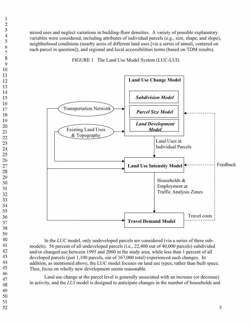
Figure 1 illustrates the relationships of various LUC-LUI model components. The LUC model anticipates how individual parcels evolve: whether an undeveloped parcel will divide into several smaller parcels during a pre-specified time interval (e.g., 5 years in this study), how big these subdivided parcels are likely to be, and what land use types will emerge on each (including undeveloped use). The likelihood of subdivision was simply modeled using a binomial logit and newly generated parcel sizes were determined using log-linear regression techniques. Land development on such previously undeveloped parcels was modeled using an MNL for various use alternatives (e.g., large lot single family, single family, multi-family, commercial or office, industrial, civic, and undeveloped). These alternatives are rather distinct; they do not include

5

mixed uses and neglect variations in building-floor densities. A variety of possible explanatory variables were considered, including attributes of individual parcels (e.g., size, shape, and slope), neighborhood conditions (nearby acres of different land uses [via a series of annuli, centered on each parcel in question]), and regional and local accessibilities terms (based on TDM results).

FIGURE 1 The Land Use Model System (LUC-LUI)

In the LUC model, only undeveloped parcels are considered (via a series of three sub-

models). 56 percent of all undeveloped parcels (i.e., 22,400 out of 40,000 parcels) subdivided and/or changed use between 1995 and 2000 in the study area, while less than 1 percent of all developed parcels (just 1,100 parcels, out of 167,000 total) experienced such changes. In addition, as mentioned above, the LUC model focuses on land use types, rather than built space. Thus, focus on wholly new development seems reasonable.

Land use change at the parcel level is generally associated with an increase (or decrease) in activity, and the LUI model is designed to anticipate changes in the number of households and

Land Use Intensity Model

Households & Employment at Traffic Analysis Zones

Transportation Network

Existing Land Uses & Topography

Feedback

Travel Demand Model

Land Use Change Model

Subdivision Model

Parcel Size Model

Land Development Model

Land Uses at Individual Parcels

Travel costs

6

employment (by type), using a seemingly unrelated regression (SUR) with two spatial processes, as follows:

( ) ( ) mmmmmmmmmmmmmm εZδεXWyβεXβWyy +=+=++= ',',ρρ (1)

mmmm ξWεε += λ (2)

where m = 1:M and indexes the four equations for each zone (i.e., counts of households and basic, retail and commercial jobs), ym is an n by 1 vector of response variables for equation m, Xm is a matrix of explanatory variables for equation m (including recent changes in land use areas, lagged counts of households and jobs, undeveloped land, land use balance and regional accessibility), βm is vector of parameters to be estimated, ρm is spatial lag autoregressive coefficient, and λm is spatial error autoregressive coefficient. The LUC and LUI model specifications are rather statistical in nature; due to space limitations, many of their details are described in Zhou and Kockelman (2008a, 2008b).

The LUC and LUI models are sequentially applied, and outputs of the LUC model (i.e., parcel-level land use changes) serve as key inputs to the LUI model (in the same model year). LUI effects filter to the LUC model in a downstream time step via regional and local accessibility variations, as anticipated by the TDM. Both land use models enjoy mechanisms to help ensure reasonable regional totals: The LUC model’s alternative-specific constants were designed to reflect regional/five-county changes, and the LUI model’s household and job forecasts were adjusted to match predetermined regional control totals (without any backwards adjustments to the LUC model). Issues with such adjustments are discussed later, in the Additional Lessons section.

DATA ISSUES Data sets for detailed models of land use systems generally come from multiple sources, and the Austin LUC-LUI application is no exception. Here, the data sets include land use parcel maps, base-year counts of households (by category) and jobs (by type) at the TAZ level, transportation network details, and topographic data. Unfortunately, land use parcel data for the entire (five-county) MSA is limited (to a single year), requiring creative treatment of estimated parameters for reasonable results when the LUC model is applied to the entire region.

In order to track the dynamics of parcel evolution, the LUC model requires parcel maps at two (or more) points in time. Only one (for the year 2005) could be obtained from the Capital Area Council of Governments (CAPCOG), who assembled the map using property appraisal data. Thus, the LUC model was estimated initially only for the City of Austin and its two-mile extraterritorial jurisdiction (ETJ) using 1995 and 2000 parcel maps. This model was then applied to the entire region’s set of year-2005 undeveloped parcels. To ensure that region-wide forecast values matched target values2 within a predefined tolerance (1 square mile per land use type in this study of a 4,280-square mile region), alternative specific constants were iteratively adjusted.

As noted earlier, the LUI model estimates changes of household and job counts (by type) across five-year time steps, based on land use changes as well as lagged values of land use intensity, undeveloped land, land use balance and regional accessibility. It should be noted that 2 The region-wide “targets” were forecasted based on 2005 land use parcel map, as well as regional household and job counts/targets for 2005 and 2010.

7

the LUI model, which relies on a SUR model with two spatial processes and a spatial weight matrix, cannot be easily extended to a larger region, with new zones added, nor some subset of zones3. For this reason, year 2000 land use conditions had to be backcasted for each TAZ, to ensure that the application set of zones matched the model estimation. Such is a limitation of various spatial econometric techniques, meriting one’s attention well before final model specification. Of course, this same guidance is true in models of all types: one should understand all modeling objectives (including policy tests and outputs of interest), data set limitations and any methodological constraints before finalizing the specification. Especially, data deficiencies present many other issues for model formulation and application, as described below.

ADDITIONAL LESSONS As alluded to above, further details on the LUC-LUI model’s specification, parameter estimates, and application results can be found in Zhou and Kockelman’s (2008d) report. For purposes of this paper, a more interesting question is how does such a model perform in practice? What deficiencies and challenges emerge, and can these be resolved?

Limits on Development and Model Extrapolations Left unchecked, models calibrated on the basis of past trends in land use change can lead to overdevelopment or underdevelopment in the future. This is particularly true in a case where more centrally located data points (e.g., parcels within the City of Austin and its ETJ) determine the specification and their parameters are “transferred” to the regional setting. While this particular scenario was avoided here in the first time step − thanks to early parameter adjustment based on a five-year target − such adjustments may be of little use over the longer term, and model estimates can take on a life of their own.

If targets are not embedded naturally into the model, post-processing is generally used, requiring heroic and unsatisfying assumptions (such as proportional adjustment of all zones’ values) in order to hit regional control totals. Here, the LUC and LUI models are sequentially applied, and forecasts of the LUI model had to be adjusted in order to ensure reasonable regional totals. Parcel subdivision and land use change could be undertaken (in random order across undeveloped zones, as is presently the case) until a certain target of total land in each use is met. But this does not guarantee that application of the subsequent LUI model will then result in reasonable household and job counts for each model year. Totals by type can get out of synch, and modelers are left with little or no recourse.

Meeting control totals is a tricky issue that deserves great care. While models like UrbanSim and LUSDR allocate jobs and households up to pre-specified targets, in each category, thus avoiding the control-totals issue. They do not enjoy endogenous determination of such quantities and rely on random order in agent assignments in each model year, thus neglecting within-year bidding competition for scarce space. In order to match regional control total expectations for Austin, the LUI model results were post-processed, in two steps. First, households and jobs were added or removed uniformly across the entire MSA (in proportion to TAZ sizes) in order to maintain their relative values. Next, unreasonable forecasts were removed using simple rules: if a zone was forecasted to have a negative count, zero values were assigned.

3 The issue in prediction essentially is that any zone’s (best) prediction depends, in a simultaneous way, on those of its neighbors, as with standard time-series data. However, prediction for a single equation has been proposed in more standard spatial auto-regressive systems (Pace and LeSage 2008).

8

Adjustment of zone-level LUC model results (by scaling land acreages up or down, according to use type) could have been pursued as well. Whichever post-processing technique is used, however, the options are unsatisfying.

Related to the idea of parameter transferability is the idea of model extrapolation − over time and space. As models move forward in time, past data sets and their parameter estimates are less and less likely to apply. Preferences evolve, along with incomes, household sizes, technologies, energy prices, and various other key inputs. As regions expand, variables and estimates that made good sense for the original region lose their value. One example is sub-center nucleation, as a previously one-center region begins to enjoy multiple centers. Another example is the variable of distances to the nearest highway. Since paired land use data sets were only available for the City of Austin and its ETJ, this variable’s maximum was originally 1.2 miles. For application of the resulting model to the larger region, the distance grew to 40.3 miles in certain cases, potentially resulting in values that dominated model results. Here, this variable was capped at 1.2 miles across all locations; no great options generally exist in such cases. Proper data sets need to be present from the start in order to avoid these kinds of questionable assumptions relatively late in the modeling process.

Implications of Model Specification for Purposes of Policy Analysis While decision-making support is the primary purpose of most LUMs, it often ends up being difficult to code a variety of land use policies in a particular model. Consider the example at hand: certain parcels can be removed from LUC consideration (due to an urban growth boundary, for example), their land use alternatives may be restricted (due to zoning, for example), or the attractiveness of their alternatives adjusted (due to subsidies for different land use types, for example); however, a sophisticated model of counts, using a spatial system of equations that share information in their error terms is not easily adapted to cases where certain zones are not allowed to experience growth in certain land use intensity values (due to zoning or other constraints) or some subset of values are otherwise pre-determined (due to prior knowledge of near-term development, for example). Spatial econometric tools are still emerging, and this challenge may one day be resolved, but in the meantime it represents a hurdle here that was unfortunately unforeseen.

The effects of transportation policies will largely depend on the accompanying TDM’s specification, and the LUM linkage. For example, variable-road pricing policies will require that time and cost metrics appropriately impact trip time of day, mode, and destination choice decisions, and that network assignment results feed back into trip distribution and other travel decisions (for consistency in sub-model assumptions and system-wide equilibration). While travel demand model specifications are largely outside the scope of this paper, it is very important to consider specification of the transportation-land use linkage, to ensure that transportation policies can affect land use patterns, if we believe that land use patterns respond in some way to transportation system conditions. Typical practice is to have regional accessibility terms feature in zone attractiveness equations for new development. In less simplistic and more spatially detailed LUMs (e.g., 150 m grid cells commonly used in UrbanSim or the parcels used here), more local transportation system attributes can be used. Here, they included parcel-based number of transit stops within 0.5 mile, network travel times to the region’s CBD, and distance to the nearest freeway.

9

Other policies of interest also exist. The proposed LUM does not consider land price signals, and is insensitive to fiscal policies, such as differential property taxation and subsidies. This could be remedied, to some extent, by controlling for neighboring parcels’ land prices in the LUC Model (to anticipate land value impacts on development decisions) and directly modeling property valuation (for price predictions across parcels in each time step).

Inclusion and Significance of Explanatory Variables This issue simply refers to the fact that various explanatory factors are not controlled for in the specification (e.g., soil quality, property tax rates, the presence of views, and school district scores). Ideally, more meaningful factors impacting land development decisions should be included, to enhance model flexibility in application. Of course, this brings us back to the very fundamental issue of data availability: someone will first need to assemble such variables for all zones/locations, trusting that these vary a fair bit across zones (which is unlikely with some variables, like construction costs, in many cases), and then hope that they emerge as statistically significant and with intuitive signs in the estimated parameter set. There are simply no guarantees that the data acquisition efforts will pay off. And it generally is enough work to acquire more basic information (like parcel location, current and past land uses, network and demographic variables, neighborhood land use conditions for each parcel, and so forth); expending constrained resources to acquire variables that may or may not offer much to the model is a real risk.

In addition, when integrating a TDM and LUM, no transportation-system variables are guaranteed to have a practically or statistically significant effect on location choice or land development patterns. Location choice is a complex decision. Land markets reflect the interacting decisions of multiple actors, and developers, households and firms are not entirely rational or well informed of their options. Moreover, reliance on cross-sectional data sets for location choices (very common in practice, due to data availability) misses true move decisions, and can lead to anomalous results (e.g., negative coefficients on regional accessibility variables), reflecting the fact that many jobs and households are entrenched in past location choices and built spaces, rather than being able to choose anew, based on rational decision-making processes, where access is thoughtfully considered. In practice, simple Euclidean distance-to-CBD metrics are often far better predictors of land values, land use change, and land use intensity than more meaningful and rigorous measures of urban form (e.g., Kockelman 1997, Bina and Kockelman 2006).

Such facts of modeling are unfortunate, but real. Many policies of interest may simply not be testable because the data sets exhibit no reasonable response to these variables or the variables do not vary over observational units to begin with (which is regularly the case with macroeconomic indicators [like interest rates] or potential policy variables that affect an entire region’s agents all at once [such as gas prices]). Moreover, many desirable data sets simply do not exist. For example, when formulating the parcel-based LUM discussed here, zoning variable simply does not exist for the entire region.

MODEL APPLICATION The above discussion illuminates many modeling issues present in various LUM paradigms, including the one used here. In applying the LUC-LUI model, coupled with a relatively standard TDM, one can illuminate even more potential issues and modeling challenges. Here, the

10

integrated LUM-TDM system was applied to anticipate the year-2030 distribution of households and jobs and travel conditions across the Austin-Round Rock MSA.

To better appreciate model sensitivities and the potential implications of different policies, two scenarios were examined: a business-as-usual (BAU) or trend scenario and a road pricing scenario. The BAU scenario assumes that development trends observed over the five-year calibration will continue, and no new policies are imposed. The road pricing scenario combines congestion pricing with a gas (or carbon) tax. A congestion charge was set to equal the implicit cost of marginal delay (imposed per added vehicle-mile-traveled, assuming a $6.75/person-hour value of travel time) on all freeway segments in the network, and the carbon tax was assumed to be 4.55 cents per mile4 on all links in the network. These two scenarios were simulated through year 2030 at five-year intervals.

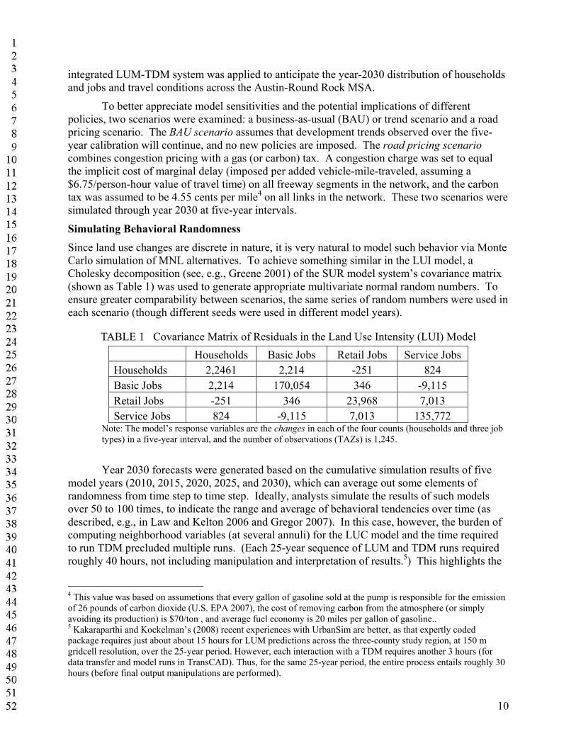
Simulating Behavioral Randomness Since land use changes are discrete in nature, it is very natural to model such behavior via Monte Carlo simulation of MNL alternatives. To achieve something similar in the LUI model, a Cholesky decomposition (see, e.g., Greene 2001) of the SUR model system’s covariance matrix (shown as Table 1) was used to generate appropriate multivariate normal random numbers. To ensure greater comparability between scenarios, the same series of random numbers were used in each scenario (though different seeds were used in different model years).

TABLE 1 Covariance Matrix of Residuals in the Land Use Intensity (LUI) Model Households Basic Jobs Retail Jobs Service Jobs Households 2,2461 2,214 -251 824 Basic Jobs 2,214 170,054 346 -9,115 Retail Jobs -251 346 23,968 7,013 Service Jobs 824 -9,115 7,013 135,772

Note: The model’s response variables are the changes in each of the four counts (households and three job types) in a five-year interval, and the number of observations (TAZs) is 1,245.

Year 2030 forecasts were generated based on the cumulative simulation results of five

model years (2010, 2015, 2020, 2025, and 2030), which can average out some elements of randomness from time step to time step. Ideally, analysts simulate the results of such models over 50 to 100 times, to indicate the range and average of behavioral tendencies over time (as described, e.g., in Law and Kelton 2006 and Gregor 2007). In this case, however, the burden of computing neighborhood variables (at several annuli) for the LUC model and the time required to run TDM precluded multiple runs. (Each 25-year sequence of LUM and TDM runs required roughly 40 hours, not including manipulation and interpretation of results.5) This highlights the

4 This value was based on assumetions that every gallon of gasoline sold at the pump is responsible for the emission of 26 pounds of carbon dioxide (U.S. EPA 2007), the cost of removing carbon from the atmosphere (or simply avoiding its production) is $70/ton , and average fuel economy is 20 miles per gallon of gasoline.. 5 Kakaraparthi and Kockelman’s (2008) recent experiences with UrbanSim are better, as that expertly coded package requires just about about 15 hours for LUM predictions across the three-county study region, at 150 m gridcell resolution, over the 25-year period. However, each interaction with a TDM requires another 3 hours (for data transfer and model runs in TransCAD). Thus, for the same 25-year period, the entire process entails roughly 30 hours (before final output manipulations are performed).

11

benefits of simpler models; while they generally come at a cost of spatial resolution as well as behavioral and/or econometric sophistication, they do offer proficient programmers an opportunity to batch run multiple scenarios (simulating variation in any number of assumptions, including policy variables, parameter estimates, and input assumptions) and offer stakeholders far more information on potential model outcomes.

Only through model application did a clear issue emerge in predictions: heteroskedasticity in job and household counts (across zones) was unaccounted for in the LUI model specification. Largely as a result of this, a couple very small TAZs (with areas of just 0.013 square mile) ended up with what appear to be excessive counts (achieving year 2030 household densities of 87 and 47 households per acre). Related to this are issues apparent in the original data sets, provided by the regional MPO: four TAZs ostensibly lost more than 500 households between 2000 and 2005 (with the biggest loss at 1645), seven lost more than 2000 basic jobs (8062 was the biggest loss) while five gained more than 2000 basic jobs (the biggest gain was 9118), and six TAZs lost more than 2000 service jobs (maximum of 4413) while four gained more than 2000 such jobs (maximum of 6277). Gaining thousands of households or jobs over a five-year period is questionable, and losing thousands is unrealistic during a period when the region is growing. While the econometrically sophisticated approach outperformed other existing model specifications (Zhou and Kockelman 2008b), such data inconsistencies can take a toll on model performance (overall R2 =0.320). Roughly, 68% of overall count variation could not be explained by the model, contributing to extreme values in simulation forecasts.

Determining New Parcel Shapes Another valuable lesson emerges in application of the parcel subdivision model. Application of the log-linear regression model of new-parcel sizes is straightforward, but providing parcel shapes is another matter.

This study used ArcGIS and MATLAB software to rasterize the parcel maps into 240 feet grid cells and then converted these maps into ASCII files for use (as a matrix) in MATLAB. MATLAB assembled 240 ft cells from left to right in each subdividing parcel, and then up to down, in order to hit predicted new-parcel sizes. This arbitrary approach resulted in new parcels with a strong east-west orientation, rather than more natural patterns of parcel formation. New parcel shaping is a difficult issue to resolve using basic mathematical techniques, but certain parallels for better models may exist in engineering studies of breakage, for example.

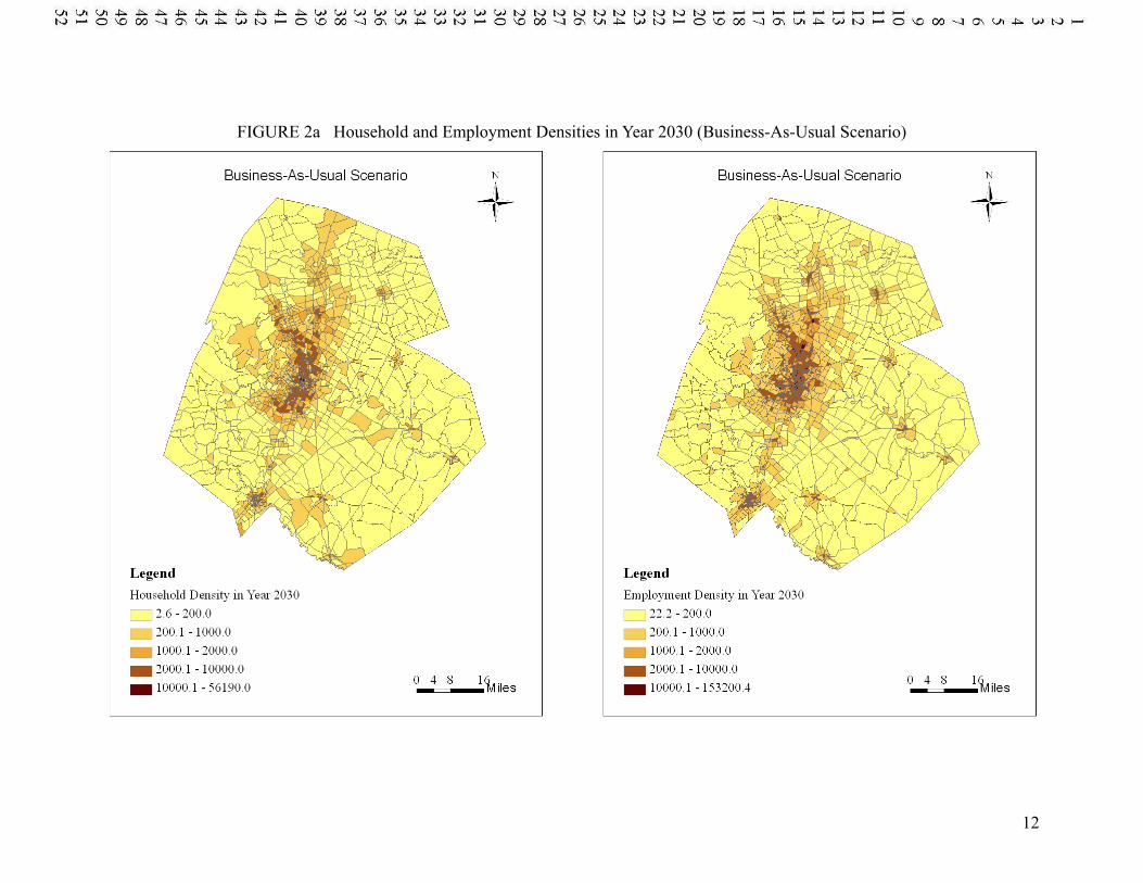
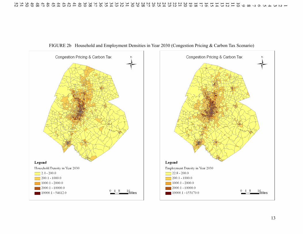
SCENARIO COMPARISONS Figure 2a and 2b show the forecasted land use intensity patterns across TAZs in year 2030 for the business-as-usual and road pricing scenarios. Both sets of predictions suggest that households and jobs tend to cluster in urban areas and along regional freeways. The road pricing scenario resulted in very similar land use patterns, indicating that the increased travel costs (averaging just 6 cents/mile) may not alter location choices, though this policy does have a significant impact on travel behavior predictions.

12

FIGURE 2a Household and Employment Densities in Year 2030 (Business-As-Usual Scenario)

13

FIGURE 2b Household and Employment Densities in Year 2030 (Congestion Pricing & Carbon Tax Scenario)

14

The count-weighted average densities for the BAU and road pricing scenarios were found to be similar: 1,568 and 1,532 households per square mile, and 6,391 and 6,375 jobs per square mile, respectively. Such minimal feedback from TDM to LUM was also found in recent application of the same scenario in a gravity-based LUM (integrated with the same TDM) for the same region (Zhou et al. 2008), supporting the notion that moderate increases in travel costs may not be reflected in land markets. The sensitivity of LUMs to TDM certainly deserves further investigation, using various modeling approaches and policy tests.

Of course, if a LUM is relatively insensitive to TDM inputs, modelers can skip the trouble of model integration and simply run the LUM forward to the future year of interest (holding accessibilities and most other transportation system variables constant), running the TDM only at the final stage. Such decisions will depend on the size and scope of transportation system changes under the scenario − and, in the hopes of urban system modelers everywhere, actual behavioral tendencies.

Regional vehicle miles traveled (VMT) is forecasted to almost double over the 25-year period, reaching 83.7 million vehicle-miles per day under the BAU scenario; but just 71.0 million/day under the road pricing scenario (a 15% reduction from the BAU total, or a 66% increase relative to base year VMT). VMT-weighted speeds and VMT-weighted volume-to-capacity ratios suggest that road pricing increases speeds about 6 percent across the region’s network during peak hours (from 50.7 to 53.9 miles/hour) while reducing average peak-period volume-to-capacity ratios by 18 percent (from 0.622 in the BAU scenario to 0.511 in the road pricing scenario).

CONCLUSIONS In order to illustrate the challenges and complexities inherent in LUM development and application, this study devised a new model of household and employment patterns, using logit models for undeveloped parcel subdivision and land use change, continuous models of new-parcel size, and a system of spatial equations for zone-level counts. While this new LUM utilizes recent advances in parcel data generation and manipulation, as well as recent innovations in spatial econometrics theory, like nearly all LUMs, it leaves much to be desired.

While various deficiencies and challenges emerged during model formulation, calibration and application, most were largely resolved via careful model specification, investigation of early forecasts, and subsequent parameter adjustments. However, others remain (such as heteroskedasticity in zone-level counts changes), resulting in certain facets of unrealistic prediction. As in nearly all LUMs, the data sets used here come from several sources, and data deficiencies are responsible for many of the issues encountered. Nevertheless, ensuring that models have a way to hit reasonable control targets (for total population and employment, for example) can be key to avoiding later (generally highly unsatisfactory) post-processing of such critical outputs. Similarly, ensuring natural mechanisms for matching supply and demand (of land and built space) can avoid a host of later problems.

Policy analysis is generally core to the development of LUMs, and policy objectives should have a significant impact on model specification, as well as estimation and application methods. Not all needs can be anticipated from the start, however, and faster model run times enjoy the advantage of facilitating diagnostic tests for model errors and timely correction of deficiencies. In general, there is much to be learned from the actual process of developing new model specifications, but all LUMs are likely to remain imperfect for the foreseeable future.

15

Nevertheless, there is much of interest and much to gain from such journeys, offering at least some insight for respective futures.

ACKNOWLEDGEMENTS The authors thank Dr. James LeSage at Texas State University for advice on prediction techniques when spatial dependent variables include both sample and ex-sample observations, Ms. Annette Perrone for her administrative assistance, and several anonymous reviewers for their comments. We also want to thank the U.S. Environmental Protection Agency STAR Grant project for financially supporting this study under Project 831183901, “Regional Development, Population Trend, and Technology Change Impacts on Future Air Pollution Emissions.”

REFERENCES Balling, R.J., J.T. Taber, M.R. Brown, and K. Day. (1999) Multi-objective Urban Planning Using

Genetic Algorithm. Journal of Urban Planning and Development, Vol. 125, No. 2, pp. 86-99.

Borning, A., P. Waddell, and R. Förster. (2007) UrbanSim: Using Simulation to Inform Public Deliberation and Decision-Making. Digital Government: Advanced Research and Case Studies, R. Traunmueller, et al. (eds.), Springer-Verlag, New York.

Clarke, K.C., S. Hoppen, and L. Gaydos. (1997) A self-modifying cellular automaton model of historical urbanization in the San Francisco Bay area. Environment and Planning B: Planning and Design, Vol. 24, pp. 247-261.

Clark, W.A.V., Huang, Y., and Withers, S. (2003) Does commuting distance matter? commuting tolerance and residential change. Regional Science and Urban Economics, Vol. 33, No. 2, pp. 199-221.

Das, D., H.H. Kelejian, and I.R. Prucha. (2003). Finite sample properties of estimators of spatial autoregressive models with autoregressive disturbances. Papers in Regional Science 82, 1–26.

Dowling, R., R. Ireson, A. Skabardonis, D. Gillen, and P. Stopher. (2005) National Cooperative Highway Research Program (NCHRP) Report 535: Predicting Air Quality Effects of Traffic-Flow Improvements: Final Report and User’s Guide. Transportation Research Board, Washington, D.C.

Greene, W. Econometric Analysis. Upper Saddle River: Prentice-Hall, 2000.

Gregor, B. (2007) The Land Use Scenario Developer (LUSDR): A Practical Land Use Model Using a Stochastic Microsimulation Framework. Transportation Research Record, 07-0438, pp. 93-102.

Hunt J.D., and J.E. Abraham. (2003) Design and application of the PECAS land use modelling system. The 8th Computers in Urban Planning and Urban Management Conference, Sendai, Japan. http://www.ucalgary.ca/~jabraham/Papers/pecas/summary.html.

Hunt J.D., J.E. Abraham, D. De Silva, M. Zhong, J. Bridges, and J. Mysko. (2008) Developing and Applying a Parcel-Level Simulation of Developer Actions in Baltimore. Proceeding of the 87th Annual Meeting of the Transportation Research Board, Washington D.C., January 2008.

16

Irwin E, and N. Bockstael. (2004) Land use externalities, open space preservation, and urban sprawl. Regional Science and Urban Economics, Vol. 34, pp. 705-725.

Johnston, R.A., and T. de la Barra. (2000) Comprehensive Regional Modeling for Long-Range Planning: Linking Integrated Urban Models and Geographic Information Systems. Transportation Research Part A: Policy and Practice, Vol. 34, No. 2, pp. 125-136.

Kakaraparthi, S., and K. Kockelman. (2008) An Application of UrbanSim to the Austin, Texas Region: Integrated-Model Forecasts for the Year 2030. Paper under review for publication in Transportation Research Record.

Kelejian, H.H., and I.R., Prucha. (2004). Estimation of simultaneous systems of spatially interrelated cross sectional equations. Journal of Economics 118, 27–50.

Kockelman, K. (1997) The Effects of Location Elements on Home Purchase Prices and Rents: Evidence from the San Francisco Bay Area, Transportation Research Record No. 1606, pp. 40-50.

Kockelman, K. M., L. Jin, Y. Zhao, and N. Ruiz-Juri (2004) Tracking Land Use, Transport, and Industrial Production using Random-Utility-Based Multizonal Input-Output Models: Applications for Texas Trade. Journal of Transport Geography, Vol. 13, No. 3, pp. 275-286.

Law, A.M., and W.D. Kelton. (2006) Simulation Modeling and Analysis, 4th Edition, McGraw-Hill Higher Education.

Lemp, J., B. Zhou, K.M. Kockelman, and B. Parmenter. (2006) Visioning vs. Modeling: Analyzing the Land Use-Transportation Futures of Urban Regions. Forthcoming in Journal of Urban Planning and Development.

McFadden, D. (1978) Modeling the Choice of Residential Location, in A. Karlquist et al. (ed.), Spatial Interaction Theory and Residential Location, North-Holland, Amsterdam.

Miller, E. J., D.S. Kriger, and J.D. Hunt. (1998) Integrated Urban Models for Simulation of Transit and Land-Use Policies: Final Report. Transit Cooperative Research Project. National Academy of Sciences.

Moeckel, R., C. Schürmann, and M. Wegener. (2002) Microsimulation of Urban Land Use. The 42nd European Congress of the Regional Science Association, Dortmund. http://www.raumplanung.uni-dortmund.de/rwp/ersa2002/cd-rom/papers/261.pdf

Parsons Brinckerhoff Quade and Douglas (PBQ&D). (1999) National Cooperative Highway Research Program (NCHRP) Report 423A: Land-Use Impacts of Transportation: A Guidebook. Transportation Research Board, Washington, D.C.

Pace, R.K., and J.P. LeSage. (2008) Spatial Econometric Models, Prediction, Encyclopedia of Geographical Information Science, Shashi Shekhar and Hui Xiong (eds.), Springer-Verlag.

PECAS (2007) Theoretical Formulation: System Documentation Technical Memorandum 1. October 2007. (Received from John Abraham in March 2008)

Raju, K.A., P.K. Sikdar, and S.L. Dhingra. (1998) Micro-simulation of residential location choice and its variation. Computers, Environment and Urban Systems, Vol. 22, No. 3, pp.

17

203-218.

Rouwendal, J., and Meijer, E. (2001) Preferences for housing, jobs, and commuting: a mixed logit analysis. Journal of Regional Science, Vol. 41, No. 3, pp. 475-505.

Silva, E.A., and K.C. Clarke. (2002) Calibration of the SLEUTH urban growth model for Lisbon and Porto, Portugal. Computers, Environment and Urban System, Vol. 26, pp. 525-552.

Syphard, A.D., K.C. Clarke, and J. Franklin. (2005) Using a cellular automaton model to forecast the effects of urban growth on habitat pattern in southern California. Ecological Complexity, Vol. 2, pp. 185-203.

Tillema, T., Ettema, D., and Van Wee, B. (2006) Road pricing and (re)location decisions of households. Proceeding of the 85th Annual Meeting of the Transportation Research Board, Washington D.C.

U.S. Environmental Protection Agency (U.S. EPA). (2000) Projecting Land-Use Change: A Summary of Models for Assessing the Effects of Community Growth and Change on Land-Use Patterns. Washington, D.C., Report EPA 600-R-00-098.

U.S. Environmental Protection Agency (U.S. EPA). (2007). Lifecycle Impacts on Fossil Energy and Greenhouse Gases. Chapter 6 of Regulatory Impact Analysis: Renewable Fuel Standard Program. Washington, D.C., Report EPA 420-R-07-004,

User Manual: TELUM (Transportation Economic and Land Use Model) Version 5.0. http://www.telus-national.org/telum/TELUMUserManual.pdf. Accessed March, 2006.

Van Ommeren, J., Rietveld, P., and Nijkamp, P. (1999) Job moving, residential moving, and commuting: a search perspective. Journal of Urban Economics, Vol. 46, No. 2, pp. 230-253.

Verburg P.H., J.R.R. Van Eck, T.C.M. Nijs, and M.J. Dijst. (2004) Determinants of land-use change patterns in the Netherlands. Environmental and Planning B, Vol. 31, pp. 125-150.

Waddell, P. (2002) UrbanSim: Modeling Urban Development for Land Use, Transportation and Environmental Planning. Journal of the American Planning Association, Vol. 68, No. 3, pp. 297-314.

Waddell, P., A., Borning, M. Noth, N. Freier, M. Becke, and G. Ulfarsson. (2003) Microsimulation of Urban Development and Location Choices: Design and Implementation of UrbanSim. Networks and Spatial Economics, Vol. 3, No. 1, pp. 43 – 67.

Waddell, P., and G.F. Ulfarsson. (2004) Introduction to Urban Simulation: Design and Development of Operational Models. In Handbook in Transport, Volume 5: Transport Geography and Spatial Systems, Stopher, Button, Kingsley, Hensher eds. Pergamon Press.

Wang, X. and K.M. Kockelman. (2006) Tracking Land Cover Change in a Mixed Logit Model: Recognizing Temporal and Spatial Effects. Transportation Research Record No. 1977, pp. 112-120.

18

Zhou, B., and K.M. Kockelman. (2008a) Neighborhood Impacts on Land Use Change: A Multinomial Logit Model of Spatial Relationships. Annals of Regional Science, Vol. 42, No. 2, pp. 321-340.

Zhou, B., and K.M. Kockelman. (2008b) Predicting the Distribution of Employment and Households: A Seemingly Unrelated Regression Model with Spatial Dependence. Forthcoming in Journal of Transport Geography.

Zhou, B., and K.M. Kockelman. (2008c) Microsimulation of Residential Land Development and Household Location Choices: Bidding for Land in Austin, Texas. Forthcoming in Transportation Research Record.

Zhou, B., and K.M. Kockelman (2008d) Predicting Land Development and Spatial Distribution of Households and Employment: An Application of a Novel Land Use Model System and Lessons Learned. Internal Report for STAR Grant program project, sponsored by the U.S. Environmental Protection Agency, at The University of Texas at Austin. Available at http://www.ce.utexas.edu/prof/kockelman/.

Zhou, B., K.M. Kockelman, and J. Lemp. (2008) Transportation and Land Use Policy Analysis Using Integrated Transport and Gravity-based Land Use Models. Proceeding of the 88th Annual Meeting of the Transportation Research Board, Washington D.C., January 2009.

LIST OF TABLES AND FIGURES TABLE 1 Covariance Matrix of Residuals in the Land Use Intensity (LUI) Model

FIGURE 1 The Land Use Model System (LUC-LUI)

FIGURE 2a Household Density in Year 2030 (Business-As-Usual Scenario)

FIGURE 2b Employment Density in Year 2030 (Business-As-Usual Scenario)

19