Lesson 7: Advanced Curve Fitting Fitting with the Two Sets of Sites

Lesson 7: Advanced Curve Fitting

55 MAU130010 Rev F-4


The model for one set of sites discussed in Lesson 1 will work for any number of sites n if all sites have the same K and ΔH. If a macromolecule has sites with two different values of K and/or ΔH, then the model with two sets of sites must be used. Whenever there are two sets of sites, the automatic initialization procedure is rarely effective. If the initialization parameters are extremely far away from best values, then convergence to the best values cannot take place as iterations proceed. In fact, often the fit gets worse rather than better with successive iterations. Therefore, the user must get involved in arriving at initialization parameters before the iterations can be started. An indication of poor initialization occurs when values for the K parameter become negative during the fitting procedure.

Fitting with the Two Sets of Sites Model

The protein ovotransferrin has two very tight, non identical sites for binding ferric ions; one located in the N domain and one in the C domain. The Origin area data FeOTF54.NDH shown below were obtained by titrating ovotransferrin with ferric ion. Injections 1-5 titrate primarily the stronger N site, injections 7-11 primarily the C site, while injections 13-15 result in no binding since both sites are already saturated. • Select File:New:Project (or click on the New Project button) to create a new

project. Click on the Read Data.. button in the RawITC window and select Area Data (*.DH) from the File of type drop down list, go to the C:\Origin70\Samples folder, and open FeOTF54.DH.

0.0 0.5 1.0 1.5 2.0 2.5 3.0

-12

-10

-8

-6

-4

-2

0

2

Feotf54_NDH

Molar Ratio

kcal

/mol

e of

inje

ctan

t

ITC Tutorial Guide

56 MAU130010 Rev F-4

• Now click on the Two sets of Sites button in the DeltaH window. Origin opens the

NonLinear Curve Fitting: Fitting Session dialog box, but produces an attention dialog box and a very poor initial fit to the curve. Click OK in the warning dialog to proceed.

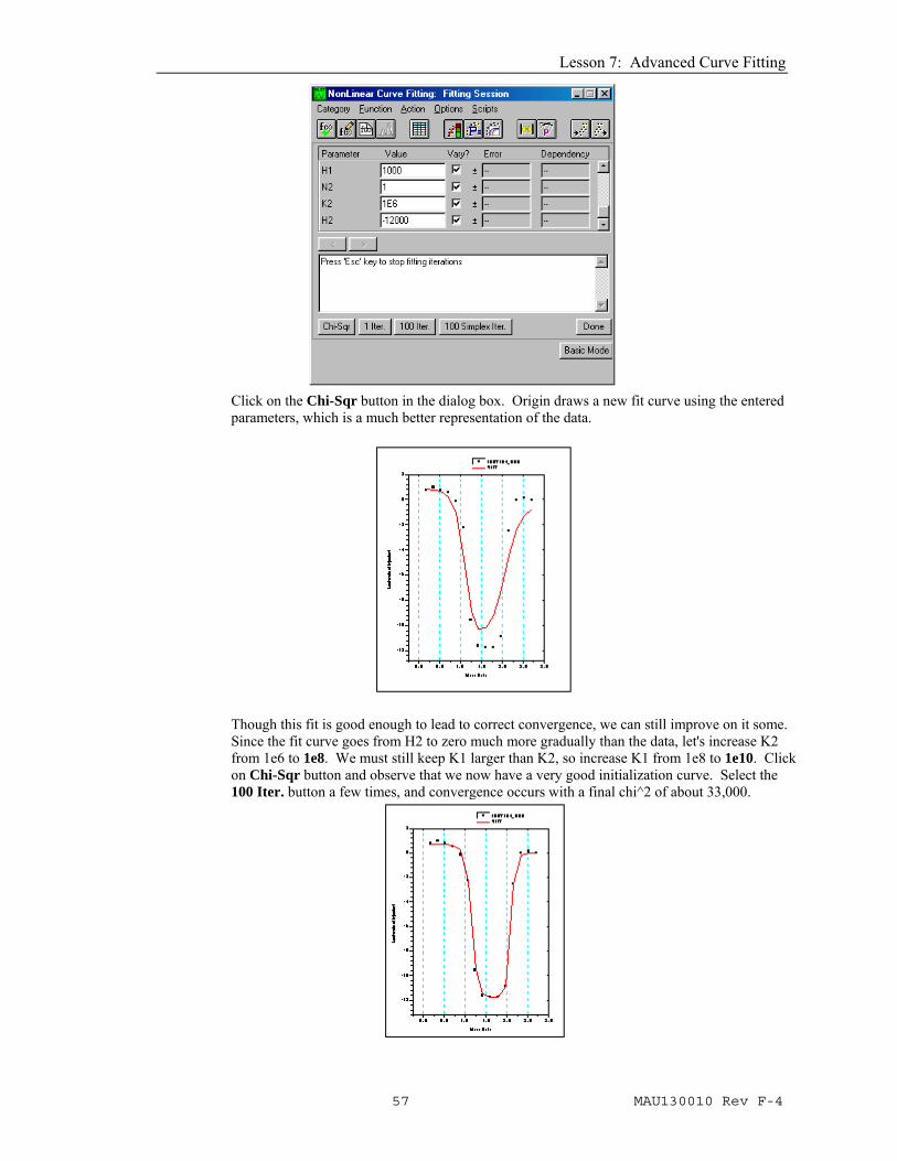
You will see that the auto initialization produces a curve which represents the data very poorly. If iterations are started from this, the fit will not converge. A little intuition, however, will allow the operator to obtain a satisfactory initialization which will lead to convergence. Examination of the experimental points shows that the first few injections at a molar ratio below 1 produce ca. 1 kcal per mole of injectant, changing to ca. -12 kcal for molar ratio 1 to 2 and finally changing to zero at molar ratios larger than 2. Begin manual initialization then by entering 1 into both the N1 and N2 parameter boxes in the Fitting Session dialog box. Because of the behavior noted above, H1 must be near +1000 and H2 close to -12,000, so enter these guesses into the appropriate parameter boxes. Since the experimental heats fall off quickly from the H1 value to the H2 value, it is clear that K1 must be much larger than K2, and because the heat changes abruptly from the H2 value to zero (i.e., beginning with the eleventh injection) it is also clear that K2 itself must be large (i.e., even though it is smaller than K1). Enter 1e8 into the K1 parameter box, and 1e6 into the K2 parameter box. Be careful not to insert a space before or after the e when using exponential notation, or Origin will not accept the value.


57 MAU130010 Rev F-4

Click on the Chi-Sqr button in the dialog box. Origin draws a new fit curve using the entered parameters, which is a much better representation of the data.

Though this fit is good enough to lead to correct convergence, we can still improve on it some. Since the fit curve goes from H2 to zero much more gradually than the data, let's increase K2 from 1e6 to 1e8. We must still keep K1 larger than K2, so increase K1 from 1e8 to 1e10. Click on Chi-Sqr button and observe that we now have a very good initialization curve. Select the 100 Iter. button a few times, and convergence occurs with a final chi^2 of about 33,000.

ITC Tutorial Guide

58 MAU130010 Rev F-4

Note that N1 and N2 are nearly the same magnitude, but not quite. It would be interesting to see if a fit of nearly equal quality could be obtained with N1 and N2 exactly equal to each other. (Although theoretically they should each be 1.0. Assign the value 1.0 into the N1 and N2 parameter value box, click in the N1 and N2 checkboxes to remove the checkmark, and continue the iterations. The final fit is not as good as when N1 and N2 are both floated, although there is no obvious explanation for this. Float all variables (by replacing the checkmark for N1 and N2) and iterate until you return to the earlier fit with a chi^2 of about 33,000. Note that sometimes you may have to click on the 10 Iter. command many times before you achieve the smallest chi^2 value, as the fitting can become trapped in a local minimum for several iterations. Click on the Done button to end the fitting session

NonLinear Least Squares Curve: Fitting Session

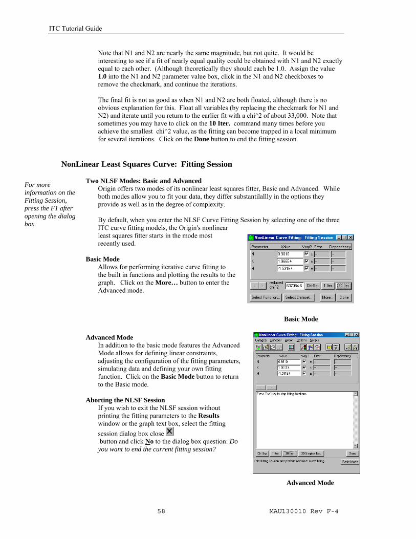
Two NLSF Modes: Basic and Advanced Origin offers two modes of its nonlinear least squares fitter, Basic and Advanced. While both modes allow you to fit your data, they differ substantilallly in the options they provide as well as in the degree of complexity.

By default, when you enter the NLSF Curve Fitting Session by selecting one of the three ITC curve fitting models, the Origin's nonlinear least squares fitter starts in the mode most recently used.

Basic Mode

Allows for performing iterative curve fitting to the built in functions and plotting the results to the graph. Click on the More… button to enter the Advanced mode.

Advanced Mode

In addition to the basic mode features the Advanced Mode allows for defining linear constraints, adjusting the configuration of the fitting parameters, simulating data and defining your own fitting function. Click on the Basic Mode button to return to the Basic mode.

Aborting the NLSF Session If you wish to exit the NLSF session without printing the fitting parameters to the Results window or the graph text box, select the fitting session dialog box close button and click No to the dialog box question: Do you want to end the current fitting session?

For more information on the Fitting Session, press the F1 after opening the dialog box.

Basic Mode

Advanced Mode


59 MAU130010 Rev F-4

Controlling the Fitting Procedure

You may enter the NLSF Curve Fitting Session and initialize the parameters by selecting one of the three fitting models (One Set of Sites, Two Sets of Sites or Sequential Binding Sites). After the parameters have been determined you may re-enter the NLSF Curve Fitting Session and keep the same fitting parameters by selecting from the menu, Math : Start Fitting Session. Normally the Fitter will open in the Basic mode, click on the More… button to enter the Advanced Mode of the Fitter. From the Fitting Session window, select Options:Control to open the Control Parameters dialog box. Edit this dialog box to specify several quantitative properties (as described below) of the fitting procedure. These properties directly affect the way the fitter performs iterations.

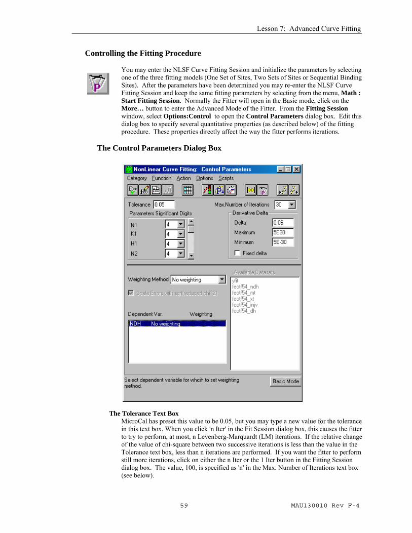
The Control Parameters Dialog Box

The Tolerance Text Box MicroCal has preset this value to be 0.05, but you may type a new value for the tolerance in this text box. When you click 'n Iter' in the Fit Session dialog box, this causes the fitter to try to perform, at most, n Levenberg-Marquardt (LM) iterations. If the relative change of the value of chi-square between two successive iterations is less than the value in the Tolerance text box, less than n iterations are performed. If you want the fitter to perform still more iterations, click on either the n Iter or the 1 Iter button in the Fitting Session dialog box. The value, 100, is specified as 'n' in the Max. Number of Iterations text box (see below).

ITC Tutorial Guide

60 MAU130010 Rev F-4

The Max. Number of Iterations Drop-down List Specify the value for the maximum number of iterations performed when the n Iter button is clicked on in the Fitting Session dialog box. This has been preset by MicroCal to be 100, but the user may change this number to be effective during a session of Origin, by entering a new value in the text box. However, the value will be reset to 100 after exiting Origin.

The Derivative Delta Group This group determines how the fitter will compute the partial derivatives with respect to parameters for ITC fitting functions during the iterative procedure. If the Fixed Delta check box is unchecked (recommended for ITC users), then the actual value of Delta (derivative step size) for a particular parameter is equal to the current value of the parameter times the value specified in the Delta text box. The Maximum and Minimum text boxes specify the limiting values of the actual Delta, in case a parameter value becomes too large or too small. MicroCal has preset the Delta to be .06 with the limiting maximum to be 5 x 10+30 and the minimum to be 5 x 10-30. If your fit curve is not converging well you may want to try a different value for the Delta, for ITC users this is typically a larger value (e.g. 0.07, 0.08, etc). The new value will be valid for the current session of Origin, but will default back to .01 the next time Origin for ITC is opened. Contact MicroCal, if you need to permanently change the Delta value.

The Parameters Significant Digits Group Select values for the display of significant digits for each parameter from the associated drop-down list. Select Free from the drop-down list to use the current Origin setting. This will only effect the text box display in the Fitting Sessions dialog box. MicroCal has preset the significant digits to be 4 for all parameters.

The Weighting Method Drop-Down List The bottom part of the Control Parameters dialog box enables you to select how different dataset points are to be weighted when computing chi-square during the iterative procedure. The choices are: No weighting, Instrumental, Statistical, Arbitrary dataset, and Direct Weighting. We recommend that the default option of No weighting be used for all ITC data unless the user has strong reason to feel another choice is more appropriate for a particular data set. No weighting assumes that each data point has the same absolute error probability. Return to the Fitting Session dialog box by clicking on the button or by selecting Action : Fit.

Deconvolution with Ligand in the Cell and Macromolecule in the Syringe

Whenever the ligand and macromolecule each have only one site for interaction with the other, then the system is symmetrical, and it does not matter which of the two is loaded into the cell and which into the injection syringe. The operator must only be careful to record the proper concentration of the species in the syringe and the species in the cell. In cases where the ligand is sparingly soluble and the macromolecule is not, then it is sometimes advantageous to load the ligand into the cell since the starting concentration then need not be so high. The situation is a little more complicated if the macromolecule has more than one site (even if there is only one set of sites). Let's assume that it has two fairly strong sites with differing affinity for ligand. If we put the macromolecule in the cell and the ligand in the


61 MAU130010 Rev F-4

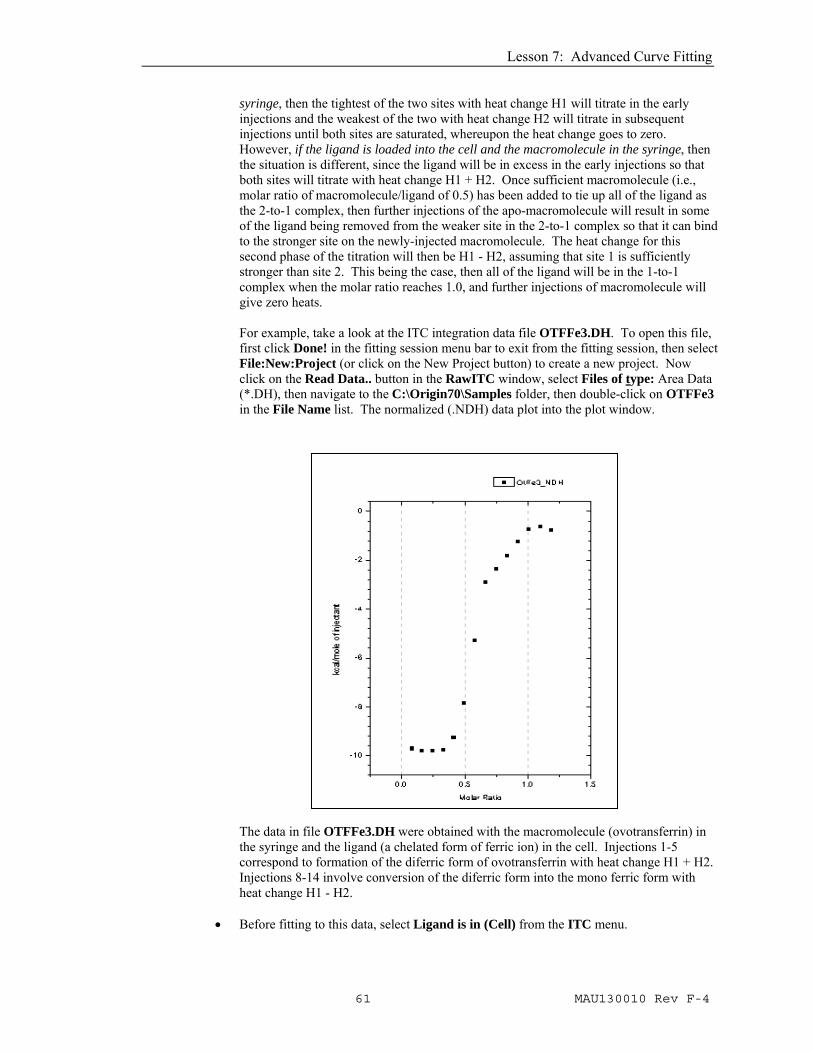
syringe, then the tightest of the two sites with heat change H1 will titrate in the early injections and the weakest of the two with heat change H2 will titrate in subsequent injections until both sites are saturated, whereupon the heat change goes to zero. However, if the ligand is loaded into the cell and the macromolecule in the syringe, then the situation is different, since the ligand will be in excess in the early injections so that both sites will titrate with heat change H1 + H2. Once sufficient macromolecule (i.e., molar ratio of macromolecule/ligand of 0.5) has been added to tie up all of the ligand as the 2-to-1 complex, then further injections of the apo-macromolecule will result in some of the ligand being removed from the weaker site in the 2-to-1 complex so that it can bind to the stronger site on the newly-injected macromolecule. The heat change for this second phase of the titration will then be H1 - H2, assuming that site 1 is sufficiently stronger than site 2. This being the case, then all of the ligand will be in the 1-to-1 complex when the molar ratio reaches 1.0, and further injections of macromolecule will give zero heats. For example, take a look at the ITC integration data file OTFFe3.DH. To open this file, first click Done! in the fitting session menu bar to exit from the fitting session, then select File:New:Project (or click on the New Project button) to create a new project. Now click on the Read Data.. button in the RawITC window, select Files of type: Area Data (*.DH), then navigate to the C:\Origin70\Samples folder, then double-click on OTFFe3 in the File Name list. The normalized (.NDH) data plot into the plot window.

The data in file OTFFe3.DH were obtained with the macromolecule (ovotransferrin) in the syringe and the ligand (a chelated form of ferric ion) in the cell. Injections 1-5 correspond to formation of the diferric form of ovotransferrin with heat change H1 + H2. Injections 8-14 involve conversion of the diferric form into the mono ferric form with heat change H1 - H2.

• Before fitting to this data, select Ligand is in (Cell) from the ITC menu.

ITC Tutorial Guide

62 MAU130010 Rev F-4

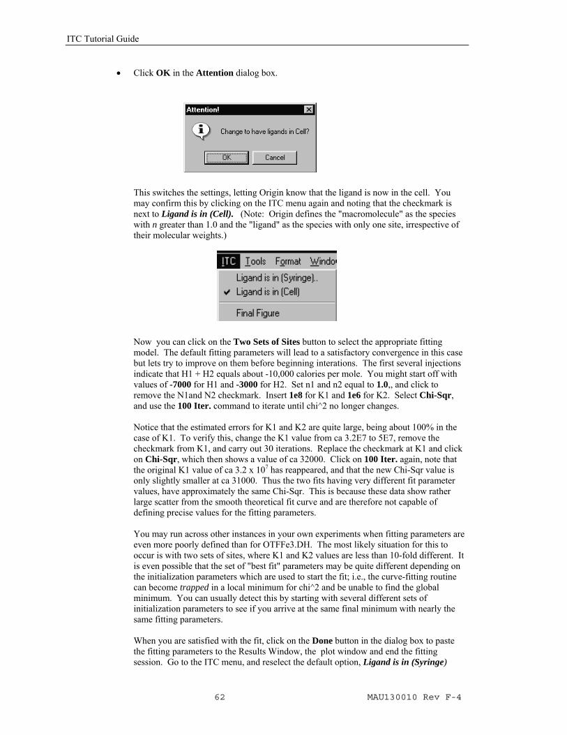
• Click OK in the Attention dialog box.

This switches the settings, letting Origin know that the ligand is now in the cell. You may confirm this by clicking on the ITC menu again and noting that the checkmark is next to Ligand is in (Cell). (Note: Origin defines the "macromolecule" as the species with n greater than 1.0 and the "ligand" as the species with only one site, irrespective of their molecular weights.)

Now you can click on the Two Sets of Sites button to select the appropriate fitting model. The default fitting parameters will lead to a satisfactory convergence in this case but lets try to improve on them before beginning interations. The first several injections indicate that H1 + H2 equals about -10,000 calories per mole. You might start off with values of -7000 for H1 and -3000 for H2. Set n1 and n2 equal to 1.0,, and click to remove the N1and N2 checkmark. Insert 1e8 for K1 and 1e6 for K2. Select Chi-Sqr, and use the 100 Iter. command to iterate until chi^2 no longer changes. Notice that the estimated errors for K1 and K2 are quite large, being about 100% in the case of K1. To verify this, change the K1 value from ca 3.2E7 to 5E7, remove the checkmark from K1, and carry out 30 iterations. Replace the checkmark at K1 and click on Chi-Sqr, which then shows a value of ca 32000. Click on 100 Iter. again, note that the original K1 value of ca 3.2 x 107 has reappeared, and that the new Chi-Sqr value is only slightly smaller at ca 31000. Thus the two fits having very different fit parameter values, have approximately the same Chi-Sqr. This is because these data show rather large scatter from the smooth theoretical fit curve and are therefore not capable of defining precise values for the fitting parameters. You may run across other instances in your own experiments when fitting parameters are even more poorly defined than for OTFFe3.DH. The most likely situation for this to occur is with two sets of sites, where K1 and K2 values are less than 10-fold different. It is even possible that the set of "best fit" parameters may be quite different depending on the initialization parameters which are used to start the fit; i.e., the curve-fitting routine can become trapped in a local minimum for chi^2 and be unable to find the global minimum. You can usually detect this by starting with several different sets of initialization parameters to see if you arrive at the same final minimum with nearly the same fitting parameters. When you are satisfied with the fit, click on the Done button in the dialog box to paste the fitting parameters to the Results Window, the plot window and end the fitting session. Go to the ITC menu, and reselect the default option, Ligand is in (Syringe)


63 MAU130010 Rev F-4

Deconvolution with the Sequential Binding Sites Model

All models discussed until now are concerned only with independent sites. It often occurs in biological systems that the binding of a ligand to one site will be influenced by whether or not ligands are bound to any of the other sites. If the sites happen to be non-identical in the first place, then binding studies alone cannot determine whether the sites are independent or interacting. On the other hand, if the sites within a molecule are known to be identical, then it is possible, sometimes, to determine if they are interacting. Consider the simplest case, that of a macromolecule with two identical sites; this might be a homodimeric protein, for example. If the sites are identical, then we can no longer distinguish between binding at the first site and binding at the second site, so the bookkeeping must be done in terms of the first ligand bound (K1, H1) and the second ligand bound (K2, H2), as described in the Appendix. A system with positive cooperativity means K2>K1, while negative cooperativity means K1>K2. Positive cooperativity is generally more difficult to distinguish from binding studies alone, since the tendency is for both sites on any single molecule to saturate together with heat change H1 + H2, so that only one "phase" is seen in the titration curve. To determine if cooperativity were present, one could use another technique which was able to show that, at half saturation, the dominant molecular forms were the macromolecule with either two or no ligands attached, with very little of the singly-liganded form. Negative cooperativity can be more easily detected from binding studies, since there will be two different "phases" occurring: the strong binding of the first ligand and the weaker binding of the second. The Origin file protb.dh shows integrated heat data on a macromolecule with two identical sites. If you have not done so yet click on Done! in the Fitting Sessions window to exit. Then select File:New:Project (or click on the New Project button) to open a new project. To open protb.dh, click on the Read Data.. button in the RawITC window, then select Area Data (*.dh) from the File of Type: drop down box. Go to the C:\Origin70\Samples sub-folder, and double-click on protb.dh.

ITC Tutorial Guide

64 MAU130010 Rev F-4

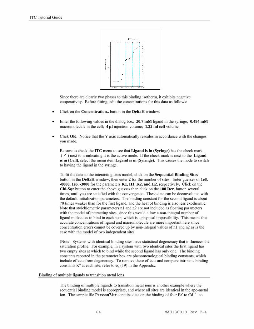
Since there are clearly two phases to this binding isotherm, it exhibits negative cooperativity. Before fitting, edit the concentrations for this data as follows:

• Click on the Concentration.. button in the DeltaH window. • Enter the following values in the dialog box: 20.7 mM ligand in the syringe; 0.494 mM

macromolecule in the cell; 4 μl injection volume; 1.32 ml cell volume.

• Click OK. Notice that the Y axis automatically rescales in accordance with the changes you made. Be sure to check the ITC menu to see that Ligand is in (Syringe) has the check mark ( ) next to it indicating it is the active mode. If the check mark is next to the Ligand is in (Cell), select the menu item Ligand is in (Syringe). This causes the mode to switch to having the ligand in the syringe. To fit the data to the interacting sites model, click on the Sequential Binding Sites button in the DeltaH window, then enter 2 for the number of sites. Enter guesses of 1e8, -8000, 1e6, -3000 for the parameters K1, H1, K2, and H2, respectively. Click on the Chi-Sqr button to enter the above guesses then click on the 100 Iter. button several times, until you are satisfied with the convergence. These data can be deconvoluted with the default initialization parameters. The binding constant for the second ligand is about 70 times weaker than for the first ligand, and the heat of binding is also less exothermic. Note that stoichiometric parameters n1 and n2 are not included as floating parameters with the model of interacting sites, since this would allow a non-integral number of ligand molecules to bind in each step, which is a physical impossibility. This means that accurate concentrations of ligand and macromolecule are more important here since concentration errors cannot be covered up by non-integral values of n1 and n2 as is the case with the model of two independent sites (Note: Systems with identical binding sites have statistical degeneracy that influences the saturation profile. For example, in a system with two identical sites the first ligand has two empty sites at which to bind while the second ligand has only one. The binding constants reported in the parameter box are phenomenological binding constants, which include effects from degeneracy. To remove these effects and compare intrinisic binding constants Ko at each site, refer to eq (19) in the Appendix.

Binding of multiple ligands to transition metal ions The binding of multiple ligands to transition metal ions is another example where the sequential binding model is appropriate, and where all sites are identical in the apo-metal ion. The sample file Persson7.itc contains data on the binding of four Br- to Cd++ to


65 MAU130010 Rev F-4

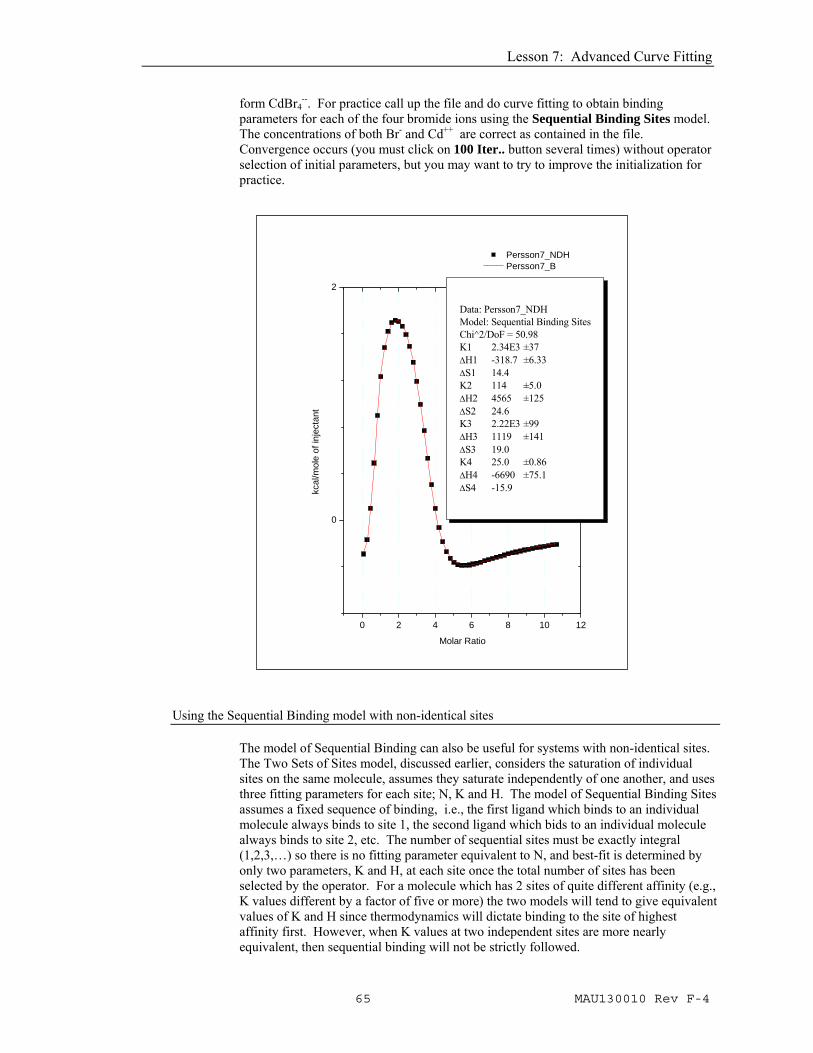
form CdBr4--. For practice call up the file and do curve fitting to obtain binding

parameters for each of the four bromide ions using the Sequential Binding Sites model. The concentrations of both Br- and Cd++ are correct as contained in the file. Convergence occurs (you must click on 100 Iter.. button several times) without operator selection of initial parameters, but you may want to try to improve the initialization for practice.

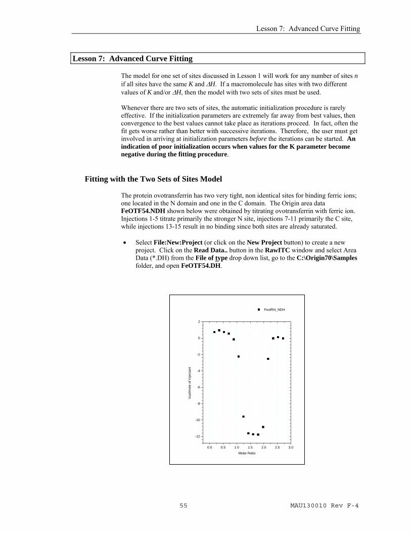
Using the Sequential Binding model with non-identical sites The model of Sequential Binding can also be useful for systems with non-identical sites. The Two Sets of Sites model, discussed earlier, considers the saturation of individual sites on the same molecule, assumes they saturate independently of one another, and uses three fitting parameters for each site; N, K and H. The model of Sequential Binding Sites assumes a fixed sequence of binding, i.e., the first ligand which binds to an individual molecule always binds to site 1, the second ligand which bids to an individual molecule always binds to site 2, etc. The number of sequential sites must be exactly integral (1,2,3,…) so there is no fitting parameter equivalent to N, and best-fit is determined by only two parameters, K and H, at each site once the total number of sites has been selected by the operator. For a molecule which has 2 sites of quite different affinity (e.g., K values different by a factor of five or more) the two models will tend to give equivalent values of K and H since thermodynamics will dictate binding to the site of highest affinity first. However, when K values at two independent sites are more nearly equivalent, then sequential binding will not be strictly followed.

0 2 4 6 8 10 12

0

2

Data: Persson7_NDHModel: Sequential Binding SitesChi^2/DoF = 50.98K1 2.34E3 ±37ΔH1 -318.7 ±6.33ΔS1 14.4K2 114 ±5.0ΔH2 4565 ±125ΔS2 24.6K3 2.22E3 ±99ΔH3 1119 ±141ΔS3 19.0K4 25.0 ±0.86ΔH4 -6690 ±75.1ΔS4 -15.9

Persson7_NDH Persson7_B

Molar Ratio

kcal

/mol

e of

inje

ctan

t

ITC Tutorial Guide

66 MAU130010 Rev F-4

One inherent advantage of the sequential model is the smaller number of fitting parameters for each site. Using a model for independent sites, it would be extremely difficult to obtain a unique fit for more than two sets of sites - which is why no fitting model for three sets of independent sites has been included in this software. As shown above for the Persson7.itc file, the sequential model is capable of providing a unique fit even for systems with four binding sites (if the K and/or H values are sufficiently different for each site). Thus, for some multi-site systems the model of sequential binding may be the only choice available for providing a unique phenomenological characterization of binding parameters..

Enzyme/substrate/inhibitor Assay

There are two different methods described below for carrying out an enzyme assay. These methods are discussed in the Appendix, where the appropriate equations are included. Both methods assume that no significant product inhibition occurs. In Method 1, an enzyme solution is in the sample cell and the experiment consists of a single injection of substrate solution into the sample cell. Immediately after injection the calorimeter baseline shifts prominently to reflect heat effects which occur from the decomposition of substrate as it comes into contact with the enzyme (because of the finite response time of the instrument, it takes a few minutes before the calorimetric signal becomes equilibrated with the actual heat from substrate turnover). Eventually, after all substrate has been reacted, the baseline will return to its original position prior to injection of substrate. From analysis of the decay curve resulting from substrate decomposition, the Michaelis parameters KM (mM)and Kcat (sec-1) may be determined as well as the heat of substrate decomposition ΔH. If a second similar experiment is carried out but with an inhibitor in the sample cell along with the enzyme, then the resulting decay curve may be analyzed in a similar way to determine the Michaelis inhibitor constant KI (mM). In the analysis of this second decay curve, the parameters determined in the first experiment (KM, Kcat and ΔH) are used as input parameters and only KI is used as a fitting parameter. In Method 2, the enzyme solution is again placed into the reaction cell but the enzyme concentration will generally be lower than in method 1. A number of injections of substrate solution are carried out, allowing baseline equilibration to occur subsequent to each injection. The equilibrated baseline value after each injection is then used to construct a plot of reaction rate versus total substrate concentration (assuming no appreciable substrate degradation takes place during measurement). From curve-fitting these data, parameters KM, Kcat, and ΔH may be determined. As in Method 1, if the experiment is repeated again but this time with added inhibitor in the enzyme solution, then the inhibitor constant KI may also be determined.

Before starting this example, you should have Origin up and running. The routines for Enzyme Assays become available after you read in the ITC data when the File of type was selected to be Enzyme Assay (*.it?).

Enzyme Assay - Method 1) Substrate Only

Begin this lesson by opening the ITC data file, M1NoInhibitor.itc, as follows:

• Select File : New : Project.

A new Origin project opens to display the RawITC plot window. • Click on the Read Data.. button.


67 MAU130010 Rev F-4

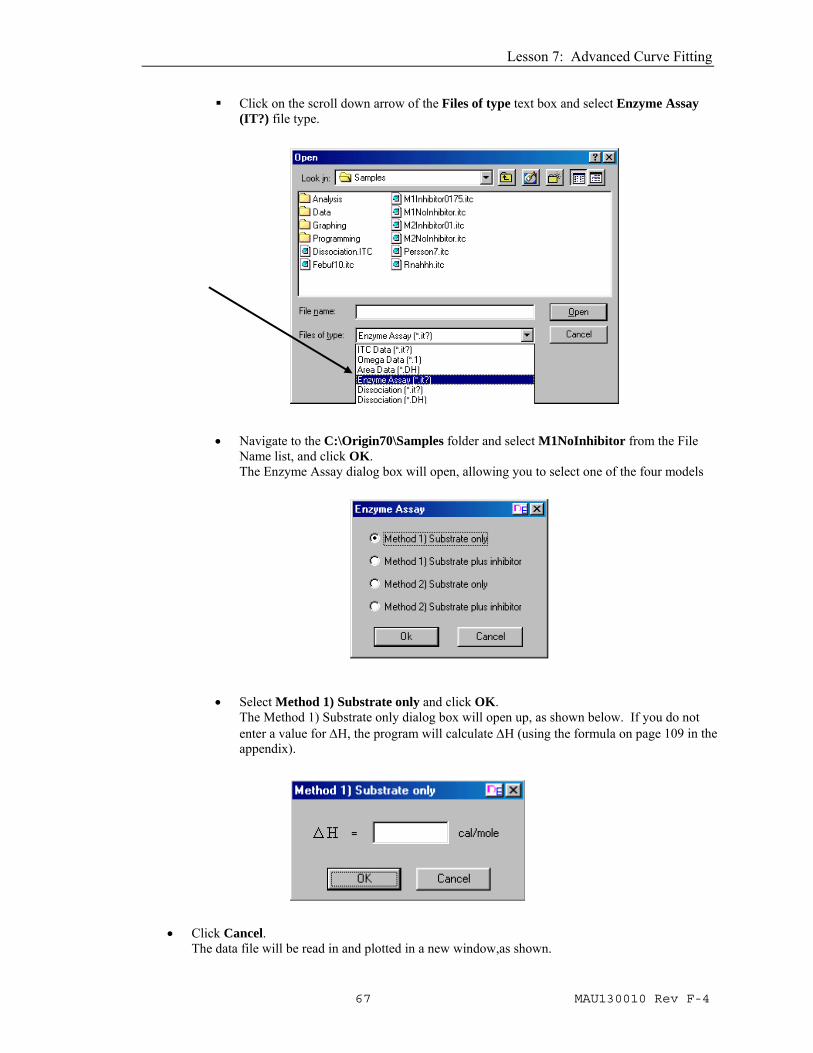
Click on the scroll down arrow of the Files of type text box and select Enzyme Assay (IT?) file type.

• Navigate to the C:\Origin70\Samples folder and select M1NoInhibitor from the File Name list, and click OK. The Enzyme Assay dialog box will open, allowing you to select one of the four models

• Select Method 1) Substrate only and click OK. The Method 1) Substrate only dialog box will open up, as shown below. If you do not enter a value for ΔH, the program will calculate ΔH (using the formula on page 109 in the appendix).

• Click Cancel. The data file will be read in and plotted in a new window,as shown.

ITC Tutorial Guide

68 MAU130010 Rev F-4

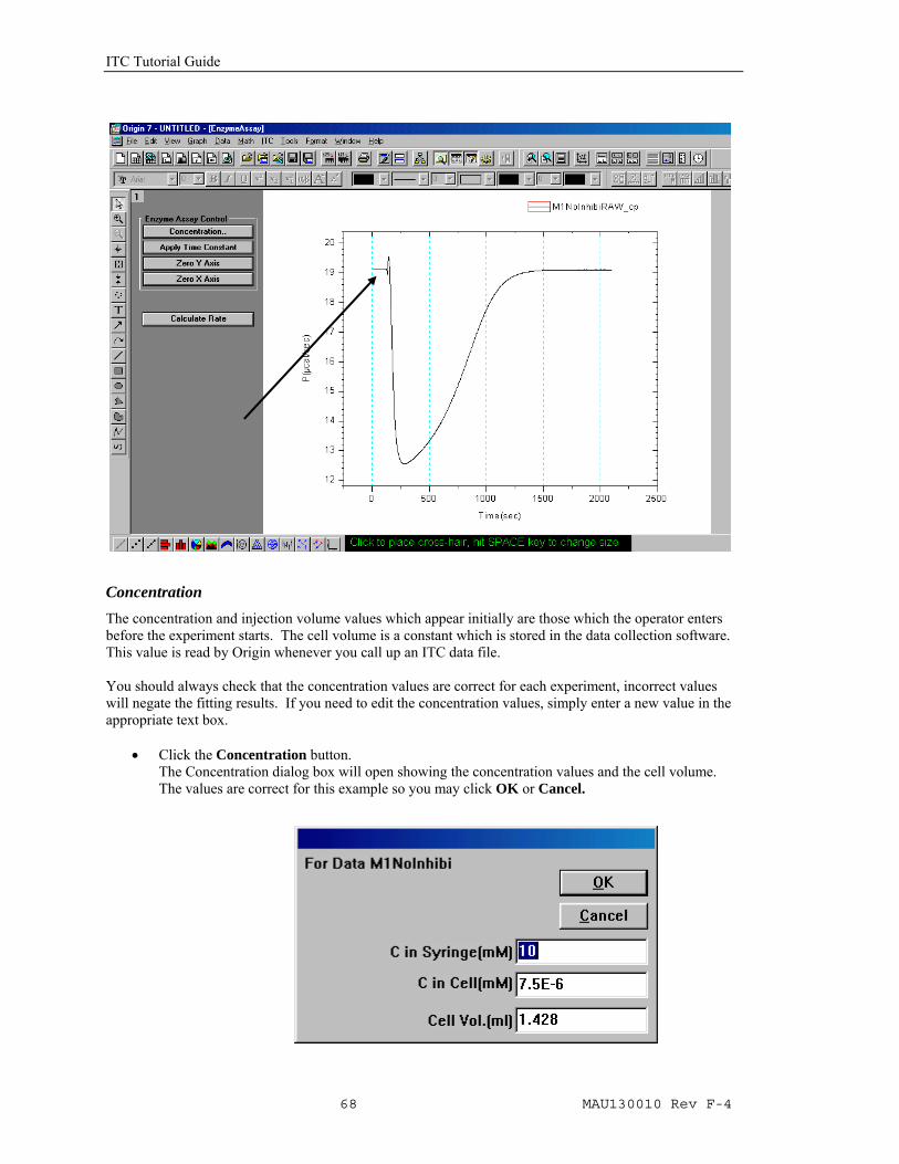
Concentration

The concentration and injection volume values which appear initially are those which the operator enters before the experiment starts. The cell volume is a constant which is stored in the data collection software. This value is read by Origin whenever you call up an ITC data file. You should always check that the concentration values are correct for each experiment, incorrect values will negate the fitting results. If you need to edit the concentration values, simply enter a new value in the appropriate text box.

• Click the Concentration button. The Concentration dialog box will open showing the concentration values and the cell volume. The values are correct for this example so you may click OK or Cancel.


69 MAU130010 Rev F-4

Apply Time Constant When substrate is injected into the enzyme solution, substrate decomposition starts to occur immediately. However, as can be seen in the figure above, it takes approximately one minute after the injection before the baseline has reached the position where it reflects the full amount of heat which is being released in the cell. This lag is caused by the finite response time of the instrument. There are two software procedures designed to reduce the effect which instrument response time exerts on final parameters obtained from the data. The first procedure is activated from the Apply Time Constant button. Knowing the actual time constant for the instrument (determined by MicroCal before shipment, and stored in Origin) the experimental data are mathematically “corrected” to remove the effect which this time constant exerted on the experimental data. When this operation is carried out, the old data is transferred out of the active window and the corrected data appears in the active window. The second procedure is activated from the Truncate Data button. Here the operator is able to remove that portion of the data immediately after the injection where distortion remains even after the time constant correction.

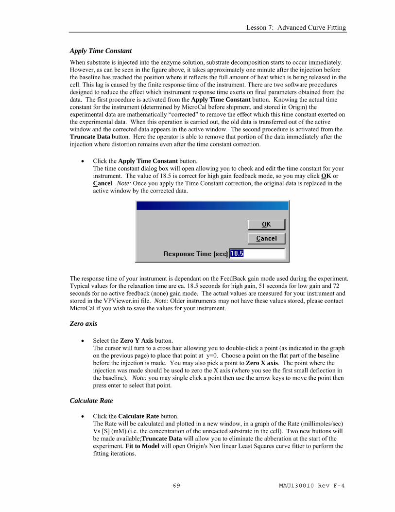
• Click the Apply Time Constant button.

The time constant dialog box will open allowing you to check and edit the time constant for your instrument. The value of 18.5 is correct for high gain feedback mode, so you may click OK or Cancel. Note: Once you apply the Time Constant correction, the original data is replaced in the active window by the corrected data.

The response time of your instrument is dependant on the FeedBack gain mode used during the experiment. Typical values for the relaxation time are ca. 18.5 seconds for high gain, 51 seconds for low gain and 72 seconds for no active feedback (none) gain mode. The actual values are measured for your instrument and stored in the VPViewer.ini file. Note: Older instruments may not have these values stored, please contact MicroCal if you wish to save the values for your instrument. Zero axis

• Select the Zero Y Axis button.

The cursor will turn to a cross hair allowing you to double-click a point (as indicated in the graph on the previous page) to place that point at y=0. Choose a point on the flat part of the baseline before the injection is made. You may also pick a point to Zero X axis. The point where the injection was made should be used to zero the X axis (where you see the first small deflection in the baseline). Note: you may single click a point then use the arrow keys to move the point then press enter to select that point.

Calculate Rate

• Click the Calculate Rate button. The Rate will be calculated and plotted in a new window, in a graph of the Rate (millimoles/sec) Vs [S] (mM) (i.e. the concentration of the unreacted substrate in the cell). Two new buttons will be made available;Truncate Data will allow you to eliminate the abberation at the start of the experiment. Fit to Model will open Origin's Non linear Least Squares curve fitter to perform the fitting iterations.

ITC Tutorial Guide

70 MAU130010 Rev F-4

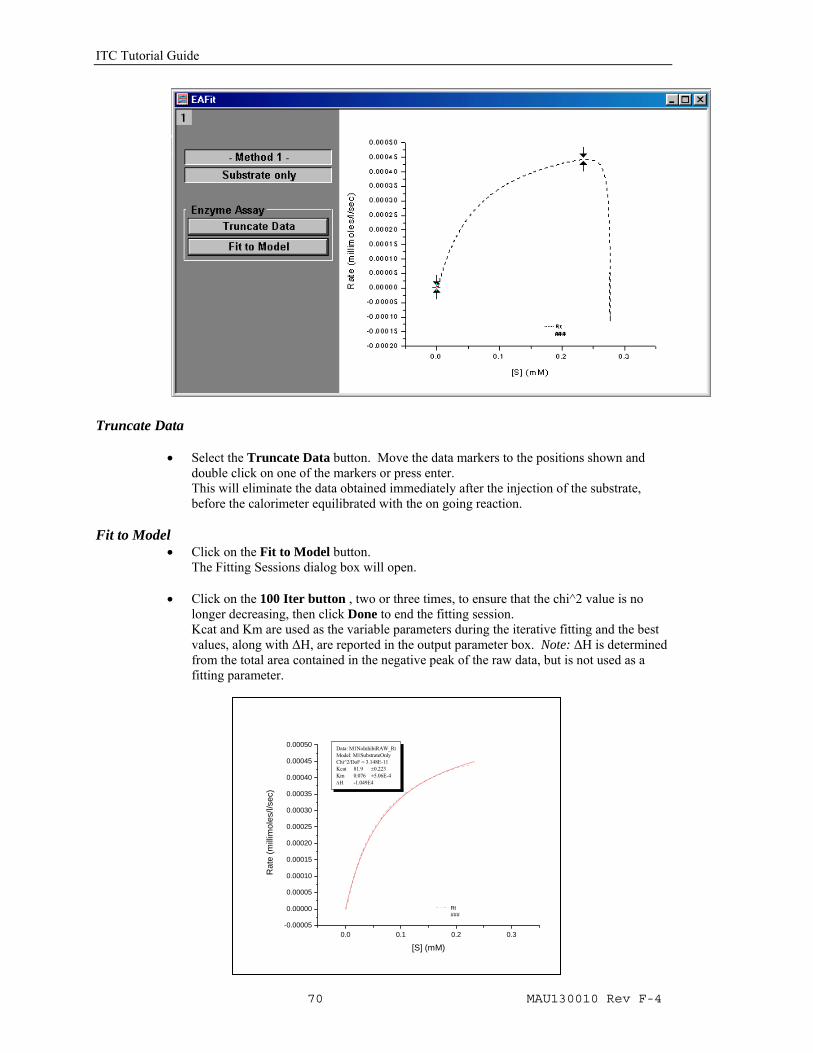
Truncate Data

• Select the Truncate Data button. Move the data markers to the positions shown and double click on one of the markers or press enter. This will eliminate the data obtained immediately after the injection of the substrate, before the calorimeter equilibrated with the on going reaction.

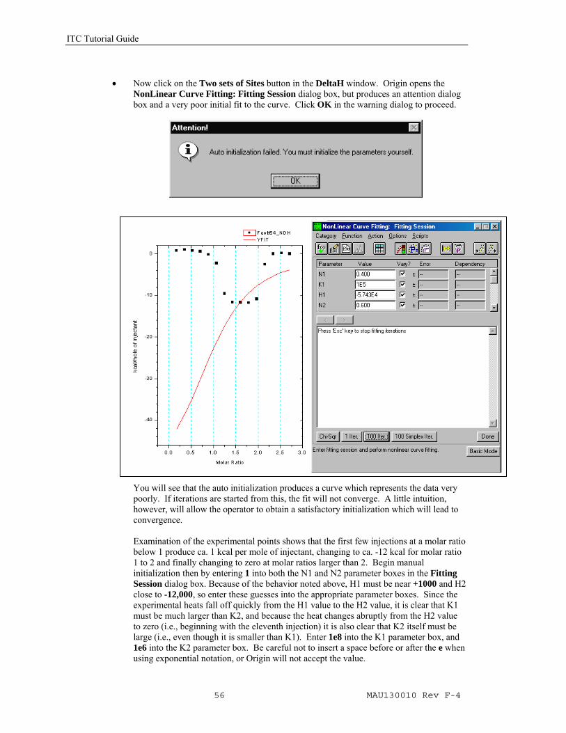
Fit to Model • Click on the Fit to Model button.

The Fitting Sessions dialog box will open.

• Click on the 100 Iter button , two or three times, to ensure that the chi^2 value is no longer decreasing, then click Done to end the fitting session. Kcat and Km are used as the variable parameters during the iterative fitting and the best values, along with ΔH, are reported in the output parameter box. Note: ΔH is determined from the total area contained in the negative peak of the raw data, but is not used as a fitting parameter.

0.0 0.1 0.2 0.3

-0.00005

0.00000

0.00005

0.00010

0.00015

0.00020

0.00025

0.00030

0.00035

0.00040

0.00045

0.00050 Data: M1NoInhibiRAW_RtModel: M1SubstrateOnlyChi^2/DoF = 3.148E-11Kcat 81.9 ±0.223Km 0.076 ±5.06E-4ΔH -1.049E4

Rt ###

Rat

e (m

illim

oles

/l/se

c)

[S] (mM)


71 MAU130010 Rev F-4

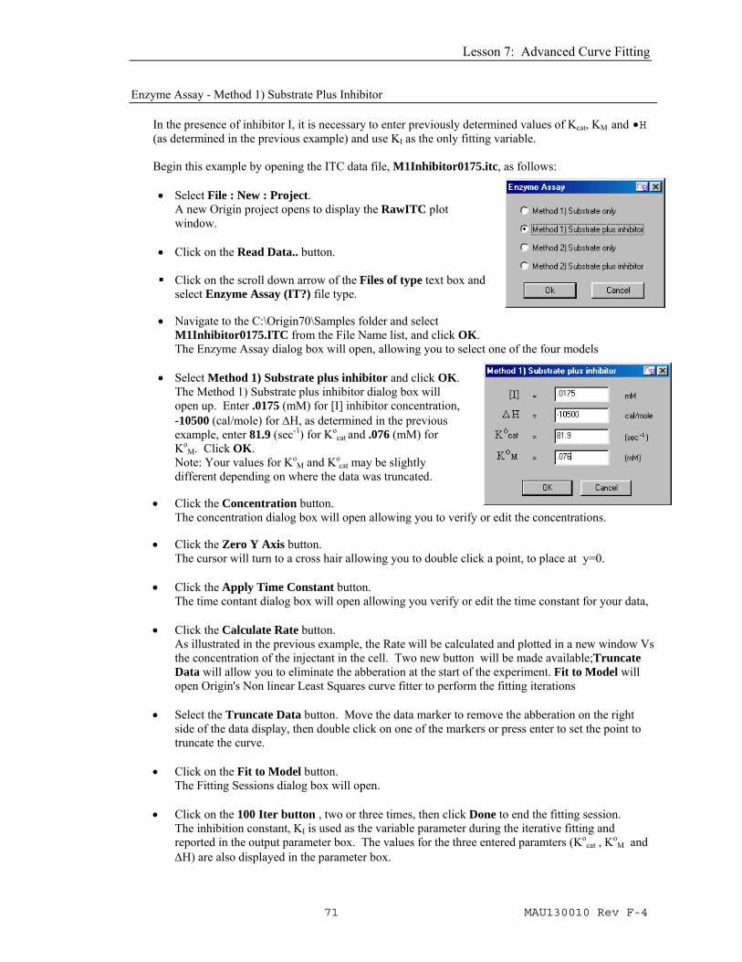
Enzyme Assay - Method 1) Substrate Plus Inhibitor

In the presence of inhibitor I, it is necessary to enter previously determined values of Kcat, KM and •H (as determined in the previous example) and use KI as the only fitting variable. Begin this example by opening the ITC data file, M1Inhibitor0175.itc, as follows:


A new Origin project opens to display the RawITC plot window.

• Click on the Read Data.. button. Click on the scroll down arrow of the Files of type text box and

select Enzyme Assay (IT?) file type. • Navigate to the C:\Origin70\Samples folder and select

M1Inhibitor0175.ITC from the File Name list, and click OK. The Enzyme Assay dialog box will open, allowing you to select one of the four models

• Select Method 1) Substrate plus inhibitor and click OK.

The Method 1) Substrate plus inhibitor dialog box will open up. Enter .0175 (mM) for [I] inhibitor concentration, -10500 (cal/mole) for ΔH, as determined in the previous example, enter 81.9 (sec-1) for Ko

cat and .076 (mM) for Ko

M. Click OK. Note: Your values for Ko

M and Kocat may be slightly

different depending on where the data was truncated.

• Click the Concentration button. The concentration dialog box will open allowing you to verify or edit the concentrations.

• Click the Zero Y Axis button.

The cursor will turn to a cross hair allowing you to double click a point, to place at y=0.

• Click the Apply Time Constant button. The time contant dialog box will open allowing you verify or edit the time constant for your data,

• Click the Calculate Rate button. As illustrated in the previous example, the Rate will be calculated and plotted in a new window Vs the concentration of the injectant in the cell. Two new button will be made available;Truncate Data will allow you to eliminate the abberation at the start of the experiment. Fit to Model will open Origin's Non linear Least Squares curve fitter to perform the fitting iterations

• Select the Truncate Data button. Move the data marker to remove the abberation on the right side of the data display, then double click on one of the markers or press enter to set the point to truncate the curve.

• Click on the Fit to Model button. The Fitting Sessions dialog box will open.

• Click on the 100 Iter button , two or three times, then click Done to end the fitting session.

The inhibition constant, KI is used as the variable parameter during the iterative fitting and reported in the output parameter box. The values for the three entered paramters (Ko

cat , KoM and

ΔH) are also displayed in the parameter box.

ITC Tutorial Guide

72 MAU130010 Rev F-4

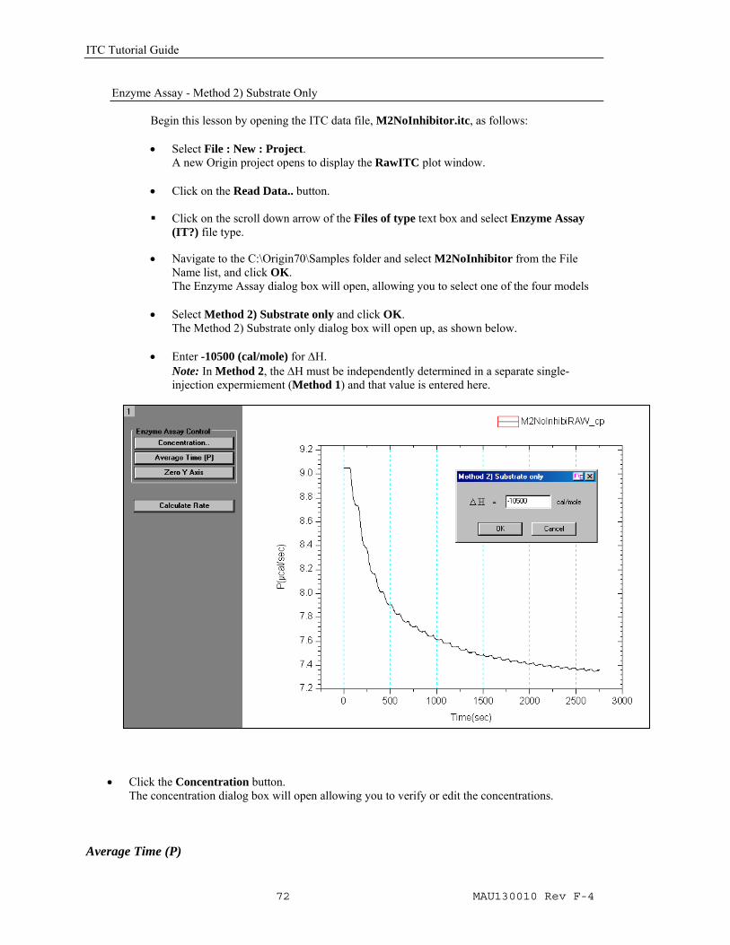
Enzyme Assay - Method 2) Substrate Only

Begin this lesson by opening the ITC data file, M2NoInhibitor.itc, as follows:

• Select File : New : Project. A new Origin project opens to display the RawITC plot window.

• Click on the Read Data.. button. Click on the scroll down arrow of the Files of type text box and select Enzyme Assay

(IT?) file type.


• Select Method 2) Substrate only and click OK. The Method 2) Substrate only dialog box will open up, as shown below.

• Enter -10500 (cal/mole) for ΔH. Note: In Method 2, the ΔH must be independently determined in a separate single-injection expermiement (Method 1) and that value is entered here.

• Click the Concentration button.

The concentration dialog box will open allowing you to verify or edit the concentrations.

Average Time (P)


73 MAU130010 Rev F-4

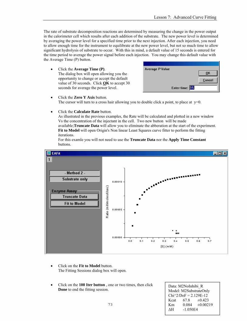
The rate of substrate decomposition reactions are determined by measuring the change in the power output in the calorimeter cell which results after each addition of the substrate. The new power level is determined by averaging the power level for a specified time prior to the next injection. After each injection, you need to allow enough time for the instrument to equilibrate at the new power level, but not so much time to allow significant hydrolysis of substrate to occur. With this in mind, a default value of 15 seconds is entered for the time period to average the power signal before each injection. You may change this default value with the Average Time (P) button.

• Click the Average Time (P). The dialog box will open allowing you the opportunity to change or accept the default value of 30 seconds. Click OK to accept 30 seconds for average the power level.

• Click the Zero Y Axis button.

The cursor will turn to a cross hair allowing you to double click a point, to place at y=0.

• Click the Calculate Rate button. As illustrated in the previous examples, the Rate will be calculated and plotted in a new window Vs the concentration of the injectant in the cell. Two new button will be made available;Truncate Data will allow you to eliminate the abberation at the start of the experiment. Fit to Model will open Origin's Non linear Least Squares curve fitter to perform the fitting iterations. For this examle you will not need to use the Truncate Data nor the Apply Time Constant buttons.


• Click on the 100 Iter button , one or two times, then click Done to end the fitting session.

Data: M2NoInhibi_R Model: M2SubstrateOnly Chi^2/DoF = 2.129E-12 Kcat 67.8 ±0.423 Km 0.084 ±0.00219 ΔH -1.050E4

ITC Tutorial Guide

74 MAU130010 Rev F-4

Kcat and Km are used as the variable parameters during the iterative fitting and , along with the entered ΔH, reported in the output parameter box.

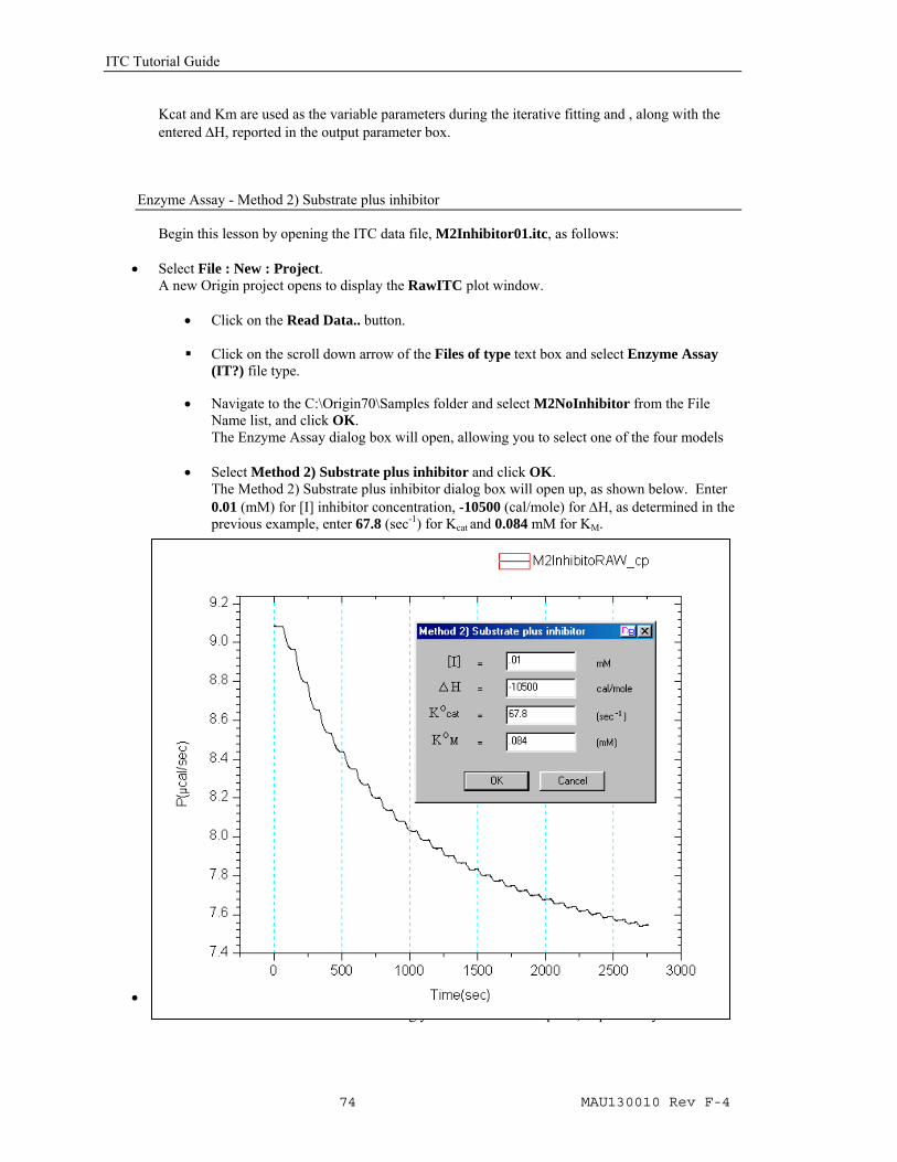
Enzyme Assay - Method 2) Substrate plus inhibitor Begin this lesson by opening the ITC data file, M2Inhibitor01.itc, as follows:


A new Origin project opens to display the RawITC plot window. • Click on the Read Data.. button. Click on the scroll down arrow of the Files of type text box and select Enzyme Assay

(IT?) file type.


• Select Method 2) Substrate plus inhibitor and click OK. The Method 2) Substrate plus inhibitor dialog box will open up, as shown below. Enter 0.01 (mM) for [I] inhibitor concentration, -10500 (cal/mole) for ΔH, as determined in the previous example, enter 67.8 (sec-1) for Kcat and 0.084 mM for KM.

• Click the Zero Y Axis button. The cursor will turn to a cross hair allowing you to double click a point, to place at y=0.


75 MAU130010 Rev F-4

• Click the Calculate Rate button. As illustrated in the previous example, the Rate will be calculated and plotted in a new window Vs the concentration of the injectant in the cell. Two new button will be made available;Truncate Data will allow you to eliminate the abberation at the start of the experiment. Fit to Model will open Origin's Non linear Least Squares curve fitter to perform the fitting iterations In Method 2, you do not need to use the Truncate Data button


• Click on the 100 Iter button , one or two times, then click Done to end the fitting session.

KI is used as the variable parameter during the iterative fitting and reported in the output parameter box. You should get a value near .0076 mM.

Dimer Dissociation Model

This model is intended for the analysis of heats of dilution data, where the sample compound in the syringe has a tendency to form dimers, i.e.,

][P[P] K 2P P

2

2H

2 ==Δ

Multiple injections are made from the syringe and the resulting heats analyzed to give best values for the dissociation constant K and the heat of dissociation ΔH.

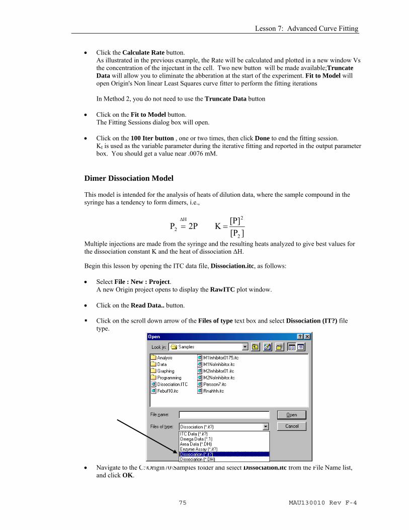
Begin this lesson by opening the ITC data file, Dissociation.itc, as follows: • Select File : New : Project.

A new Origin project opens to display the RawITC plot window. • Click on the Read Data.. button. Click on the scroll down arrow of the Files of type text box and select Dissociation (IT?) file

type.

• Navigate to the C:\Origin70\Samples folder and select Dissociation.itc from the File Name list, and click OK.

ITC Tutorial Guide

76 MAU130010 Rev F-4

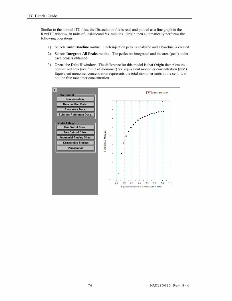
Similar to the normal ITC files, the Dissociation file is read and plotted as a line graph in the RawITC window, in units of µcal/second Vs. minutes. Origin then automatically performs the following operations:

1) Selects Auto Baseline routine. Each injection peak is analyzed and a baseline is created

2) Selects Integrate All Peaks routine. The peaks are integrated and the area (µcal) under each peak is obtained.

3) Opens the DeltaH window. The difference for this model is that Origin then plots the normalized area (kcal/mole of monomer) Vs. equivalent monomer concentration (mM). Equivalent monomer concentration represents the total monomer units in the cell. It is not the free monomer concentration.


77 MAU130010 Rev F-4

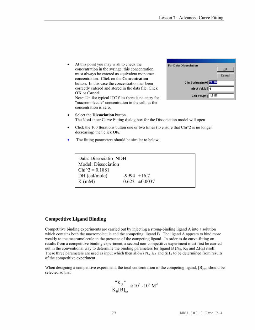
• At this point you may wish to check the concentration in the syringe, this concentration must always be entered as equivalent monomer concentration. Click on the Concentration button. In this case the concentration has been correctly entered and stored in the data file. Click OK or Cancel. Note: Unlike typical ITC files there is no entry for "macromolecule" concentration in the cell, as the concentration is zero.

• Select the Dissociation button. The NonLinear Curve Fitting dialog box for the Dissociation model will open

• Click the 100 Iterations button one or two times (to ensure that Chi^2 is no longer decreasing) then click OK.

• The fitting parameters should be similar to below.

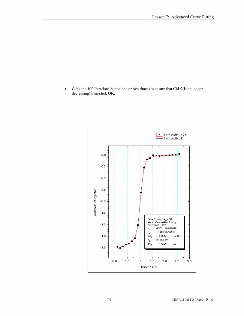
Competitive Ligand Binding

Competitive binding experiments are carried out by injecting a strong-binding ligand A into a solution which contains both the macromolecule and the competing ligand B. The ligand A appears to bind more weakly to the macromolecule in the presence of the competing ligand. In order to do curve-fitting on results from a competitive binding experiment, a second non-competitive experiment must first be carried out in the conventional way to determine the binding parameters for ligand B (NB, KB and ΔHB) itself. These three parameters are used as input which then allows NA, KA and ΔHA to be determined from results of the competitive experiment. When designing a competitive experiment, the total concentration of the competing ligand, [B]tot, should be selected so that

1-85

totB

A M 10- 10 B][K

"K"≅

Data: Dissociatio_NDH Model: Dissociation Chi^2 = 0.1881 DH (cal/mole) -9994 ±16.7 K (mM) 0.623 ±0.0037

ITC Tutorial Guide

78 MAU130010 Rev F-4

where “KA” is the estimated value of KA. This insures that the apparent binding constant in the competitive experiment will be in the best “window”, 105 to 108 M-1, to be easily measured by ITC. In the following example, results from a conventional, non-competitive experiment have already been analyzed to obtain the parameters NB=0.993, KB=21600 M-1 and ΔHB= -11700 cal/mole. The data from the competitive experiment have been saved in an area data file named Competitive.dH which will be analyzed below. Begin this lesson by opening the ITC data file, Competitive.dH, as follows:


A new Origin project opens to display the RawITC plot window. • Click on the Read Data.. button. Click on the scroll down arrow of the Files of type text box and select Area Data (*.DH) file type.

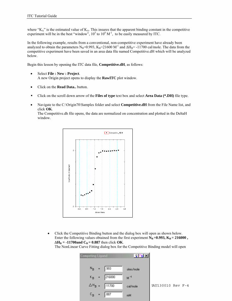
• Navigate to the C:\Origin70\Samples folder and select Competitive.dH from the File Name list, and

click OK. The Competitive.dh file opens, the data are normalized on concentration and plotted in the DeltaH window.

• Click the Competitive Binding button and the dialog box will open as shown below. Enter the following values obtained from the first experiment NB =0.993, KB = 216000 , ΔHB = -11700and CB = 0.887 then click OK. The NonLinear Curve Fitting dialog box for the Competitive Binding model will open


79 MAU130010 Rev F-4

• Click the 100 Iterations button one or two times (to ensure that Chi^2 is no longer decreasing) then click OK.

ITC Tutorial Guide

80 MAU130010 Rev F-4

Simulating Curves

You may want to simulate titration experiments without actually going through the fitting routine. The simulated curve may or may not be related to actual data which you have obtained. To simulate data, there must be some ITC results in computer memory (either raw data called up, or an Origin project that contains data) but these results need not be related to the simulations you carry out. The data in memory needs to contain at least as many data points (or number of injections) as the curve you wish to simulate (Note: for proper simulation you must use a data file that had all injections of the same volume, so do not use a file which used a preliminary 1st injection of a different size.)

To simulate a fit curve • Exit the fitting session and start a new project by selecting File:New:Project (or click on

the New Project button) from the menu. Click on the Read Data.. button in the RawITC window and select ITC Data (*.ITC) from the List Files As type box, and open the Rnahhh.ITC data file located in the [Origin70][samples] folder (alternatively you may read in the Area Data (*.dh) data file, Rnahhh.dh). The DeltaH window becomes the active window.

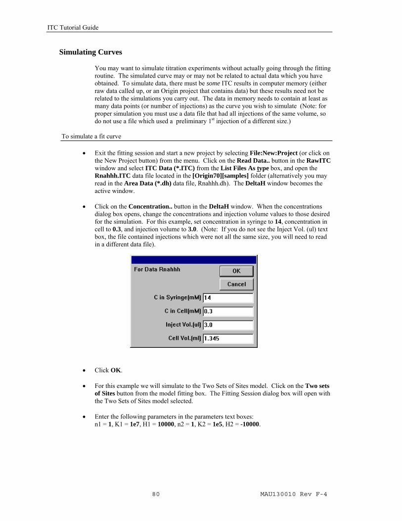
• Click on the Concentration.. button in the DeltaH window. When the concentrations dialog box opens, change the concentrations and injection volume values to those desired for the simulation. For this example, set concentration in syringe to 14, concentration in cell to 0.3, and injection volume to 3.0. (Note: If you do not see the Inject Vol. (ul) text box, the file contained injections which were not all the same size, you will need to read in a different data file).

• Click OK.

• For this example we will simulate to the Two Sets of Sites model. Click on the Two sets of Sites button from the model fitting box. The Fitting Session dialog box will open with the Two Sets of Sites model selected.

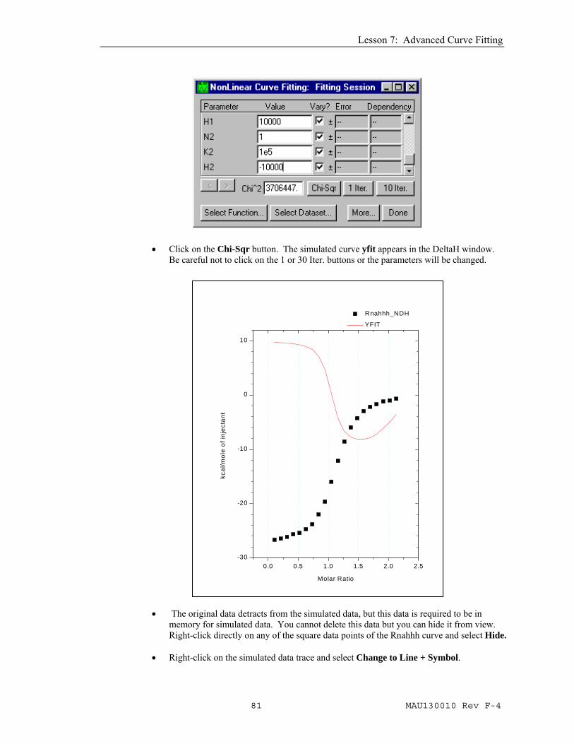
• Enter the following parameters in the parameters text boxes: n1 = 1, K1 = 1e7, H1 = 10000, n2 = 1, K2 = 1e5, H2 = -10000.


81 MAU130010 Rev F-4

• Click on the Chi-Sqr button. The simulated curve yfit appears in the DeltaH window.

Be careful not to click on the 1 or 30 Iter. buttons or the parameters will be changed.

• The original data detracts from the simulated data, but this data is required to be in

memory for simulated data. You cannot delete this data but you can hide it from view. Right-click directly on any of the square data points of the Rnahhh curve and select Hide.

• Right-click on the simulated data trace and select Change to Line + Symbol.

0.0 0.5 1.0 1.5 2.0 2.5-30

-20

-10

0

10

Rnahhh_NDH

YFIT

Molar Ratio

kcal

/mol

e of

inje

ctan

t

ITC Tutorial Guide

82 MAU130010 Rev F-4

Notice that the simulated data has twenty data points, the same as the original Rnahhh curve. Also it appears that the simulated curve has not leveled due to complete binding. This can be corrected by clicking on the Concentration.. button to increase the concentration in the syringe, decrease the concentration in the cell or increasing the volume of the injection. Alternatively you could start over and read in a data set with more data points (or injections).

• Select Window : DeltaH then click on the Concentrations button. Enter .2 mM for the

concentration in the cell. The graph will rescale on the X-axis, but the simulated curve will not be affected until you click on the Chi-Sqr button again.

• Click on the Chi-Sqr button. The curve will be simulated using the new concentration.

Using Macromolecule Concentration, rather than n, as a Fitting Parameter

In some instances, you may know the value for the stoichiometric parameter n from independent studies, but are not able to come up with an accurate estimate for macromolecule concentration Mt (Sigurskjold, Altman & Bundle (1991) Eur. J. Biochem. 197, 239-246.). Using Origin, it is an easy matter to determine Mt (along with the correct binding constant and heat of binding) from curve-fitting. The procedure is as follows: 1.) Guess at the macromolecular concentration and enter this incorrect concentration, Mt*, into the Concentration dialog box. 2.) Select the model for curve-fitting and proceed to find the best fit in the usual way. The values which you obtain for the binding constant and heat of binding will be correct since these depend only on the accuracy of the ligand concentration. However, the best value which appears for the stochiometric parameter, n*, will be incorrect since you wish to assign this yourself and, after making the correct assignment n, to determine the actual Mt. 3.) Once curve-fitting is completed, you may calculate the correct Mt which is equal to the incorrect concentration Mt* times the ratio n*/n. You may satisfy yourself that the above procedure is correct by calling the RNAHHH.ITC data into Origin, do curve-fitting using the correct concentration, and record the best values of parameters n, K and H as the correct values. Now, change the concentration by multiplying the correct concentration in the cell by 2 and enter that incorrect value into the Concentration dialog box. Do curve-fitting again and you will see that the new, incorrect value of n is exactly 50% of the correct value obtained using the correct concentration! The values for binding constant and heat of binding will be the same in the two cases.

Single Injection Method

The VP- ITC is also capable of carrying out a complete binding experiment using only a single continuous injection as opposed to the normal procedure which requires multiple injections. In this single-injection procedure, only one slow, continuous injection of


83 MAU130010 Rev F-4

ligand solution is made from the injection syringe into the macromolecule solution contained in the sample cell. It should be pointed out that the binding parameters obtained from a well designed multiple injection experiment usually have higher degree of accuracy than the single injection experiment. If the sample turnover rate is not a prime concern users should perform the multiple injection experiment for more precise binding parameters.

Correction of Raw Data for time constant of the instrument, etc. There are several operations which are automatically performed by Origin when the data file is opened : a) data corrected for the time constant of the instrument. and b) corrected data set is filtered using the standard Fourier transform filter in Origin 7.0 and a bandwidth of 15 data points. The user then a) sets the “zero baseline” from which the experimental data will be subtracted. (page 84-85), and b) exclude distorted or extraneous data points prior to subsequent analysis (page 86).

Creating New Worksheet. The raw data (after time constant correction, Fourier filtering, baseline subtraction, and eliminating inappropriate data) can then be used to form a new worksheet which is modeled after the existing worksheet used with multi-injection binding data.

To create SIM ITC icon on desktop

• Right-click any Origin 7 icon on the desktop • Choose Copy, then right-click mouse on desktop and choose Paste to create copy of Origin 7

icon. • Rename icon: Right-click the copy of the icon, choose Rename, and enter SIM ITC.

• Change target of desktop icon to SIM: Right-click SIM ITC icon, choose Properties. In Target

window, change final number of target to 8, enter OK.

To input SIM data

• Double-click SIM ITC icon on desktop.

• Click on the Read Data button in the Single Injection group

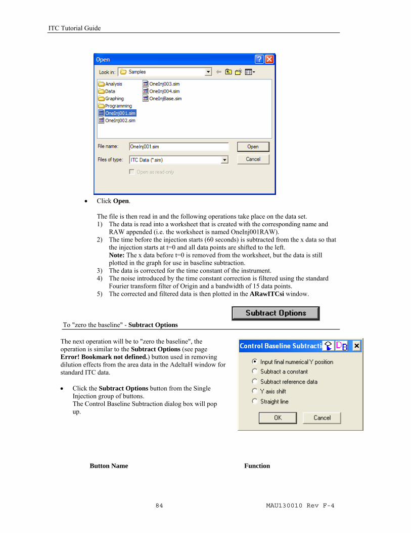
The Import Multiple ASCII dialog box opens. The only option for Files of type is ITC Data (*.sim). Navigate to the C:\Origin70\Samples folder, and then select OneInj001.sim from the Files list.

Please Note: Raw data file names should not begin with a number, nor should they contain any hyphens, periods or spaces.

ITC Tutorial Guide

84 MAU130010 Rev F-4

• Click Open. The file is then read in and the following operations take place on the data set. 1) The data is read into a worksheet that is created with the corresponding name and

RAW appended (i.e. the worksheet is named OneInj001RAW). 2) The time before the injection starts (60 seconds) is subtracted from the x data so that

the injection starts at t=0 and all data points are shifted to the left. Note: The x data before t=0 is removed from the worksheet, but the data is still plotted in the graph for use in baseline subtraction.

3) The data is corrected for the time constant of the instrument. 4) The noise introduced by the time constant correction is filtered using the standard

Fourier transform filter of Origin and a bandwidth of 15 data points. 5) The corrected and filtered data is then plotted in the ARawITCsi window.

To "zero the baseline" - Subtract Options

The next operation will be to "zero the baseline", the operation is similar to the Subtract Options (see page Error! Bookmark not defined.) button used in removing dilution effects from the area data in the AdeltaH window for standard ITC data. • Click the Subtract Options button from the Single

Injection group of buttons. The Control Baseline Subtraction dialog box will pop up.

Button Name Function


85 MAU130010 Rev F-4

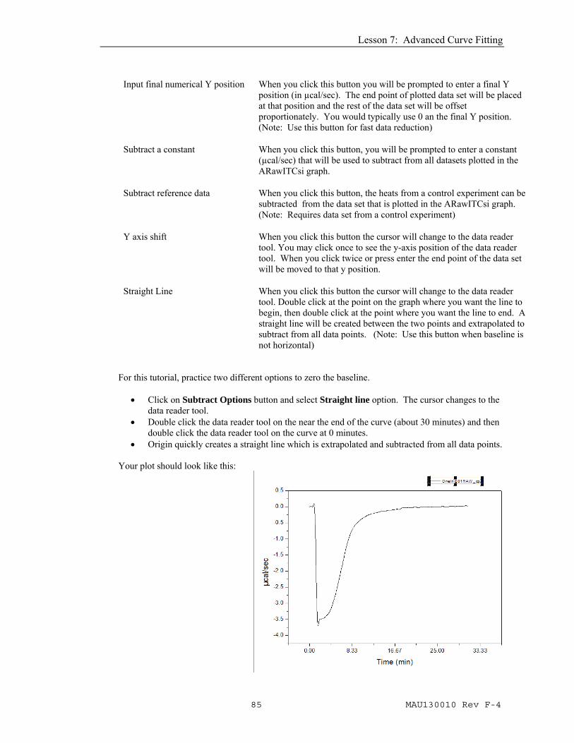
Input final numerical Y position

When you click this button you will be prompted to enter a final Y position (in µcal/sec). The end point of plotted data set will be placed at that position and the rest of the data set will be offset proportionately. You would typically use 0 an the final Y position. (Note: Use this button for fast data reduction)

Subtract a constant When you click this button, you will be prompted to enter a constant (µcal/sec) that will be used to subtract from all datasets plotted in the ARawITCsi graph.

Subtract reference data When you click this button, the heats from a control experiment can be subtracted from the data set that is plotted in the ARawITCsi graph. (Note: Requires data set from a control experiment)

Y axis shift When you click this button the cursor will change to the data reader tool. You may click once to see the y-axis position of the data reader tool. When you click twice or press enter the end point of the data set will be moved to that y position.

Straight Line When you click this button the cursor will change to the data reader tool. Double click at the point on the graph where you want the line to begin, then double click at the point where you want the line to end. A straight line will be created between the two points and extrapolated to subtract from all data points. (Note: Use this button when baseline is not horizontal)

For this tutorial, practice two different options to zero the baseline.

• Click on Subtract Options button and select Straight line option. The cursor changes to the data reader tool.

• Double click the data reader tool on the near the end of the curve (about 30 minutes) and then double click the data reader tool on the curve at 0 minutes.

• Origin quickly creates a straight line which is extrapolated and subtracted from all data points. Your plot should look like this:

ITC Tutorial Guide

86 MAU130010 Rev F-4

Hint: When moving a data marker you may press the space bar to increase the size of the cross-hair

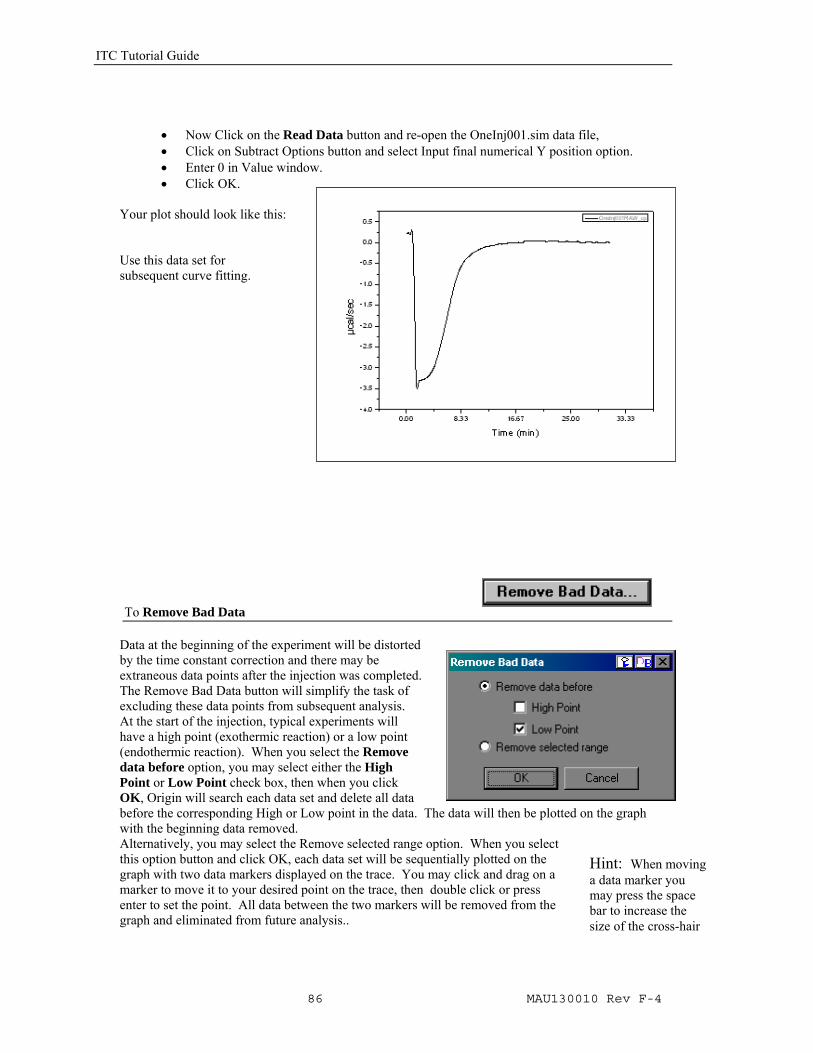
• Now Click on the Read Data button and re-open the OneInj001.sim data file, • Click on Subtract Options button and select Input final numerical Y position option. • Enter 0 in Value window. • Click OK.

Your plot should look like this: Use this data set for subsequent curve fitting. To Remove Bad Data

Data at the beginning of the experiment will be distorted by the time constant correction and there may be extraneous data points after the injection was completed. The Remove Bad Data button will simplify the task of excluding these data points from subsequent analysis. At the start of the injection, typical experiments will have a high point (exothermic reaction) or a low point (endothermic reaction). When you select the Remove data before option, you may select either the High Point or Low Point check box, then when you click OK, Origin will search each data set and delete all data before the corresponding High or Low point in the data. The data will then be plotted on the graph with the beginning data removed. Alternatively, you may select the Remove selected range option. When you select this option button and click OK, each data set will be sequentially plotted on the graph with two data markers displayed on the trace. You may click and drag on a marker to move it to your desired point on the trace, then double click or press enter to set the point. All data between the two markers will be removed from the graph and eliminated from future analysis..


87 MAU130010 Rev F-4

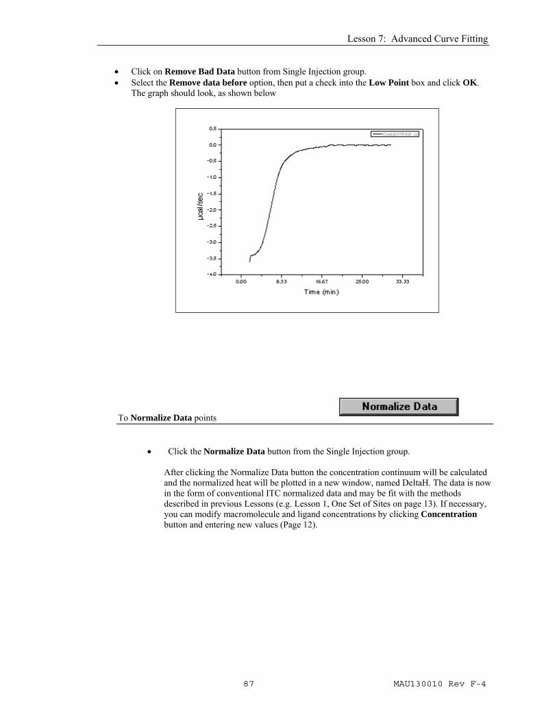
• Click on Remove Bad Data button from Single Injection group. • Select the Remove data before option, then put a check into the Low Point box and click OK.

The graph should look, as shown below

To Normalize Data points

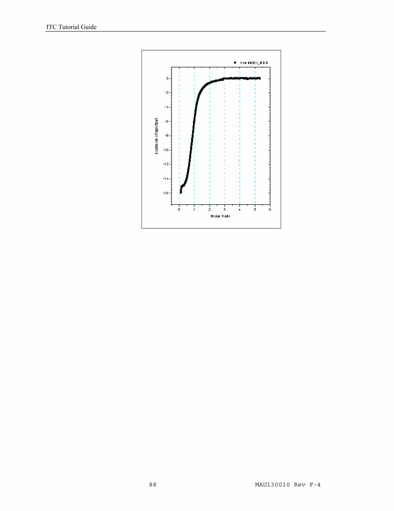
• Click the Normalize Data button from the Single Injection group. After clicking the Normalize Data button the concentration continuum will be calculated and the normalized heat will be plotted in a new window, named DeltaH. The data is now in the form of conventional ITC normalized data and may be fit with the methods described in previous Lessons (e.g. Lesson 1, One Set of Sites on page 13). If necessary, you can modify macromolecule and ligand concentrations by clicking Concentration button and entering new values (Page 12).

ITC Tutorial Guide

88 MAU130010 Rev F-4

Documents

Lesson 7: Advanced Curve Fitting Fitting with the Two Sets of Sites