Lesson-11: Study of DC transients in circuits...Module 3 DC Transient Version 2 EE IIT, Kharagpur Lesson 11 Study of DC transients in R-L-C Circuits Version 2 EE IIT, Kharagpur Objectives

Module 3

DC Transient

Version 2 EE IIT, Kharagpur

Lesson 11

Study of DC transients in R-L-C Circuits


Objectives • Be able to write differential equation for a dc circuits containing two storage

elements in presence of a resistance. • To develop a thorough understanding how to find the complete solution of second

order differential equation that arises from a simple R L C− − circuit. • To understand the meaning of the terms (i) overdamped (ii) criticallydamped, and

(iii) underdamped in context with a second order dynamic system. • Be able to understand some terminologies that are highly linked with the

performance of a second order system. L.11.1 Introduction In the preceding lesson, our discussion focused extensively on dc circuits having resistances with either inductor ( ) or capacitor ( ) (i.e., single storage element) but not both. Dynamic response of such first order system has been studied and discussed in detail. The presence of resistance, inductance, and capacitance in the dc circuit introduces at least a second order differential equation or by two simultaneous coupled linear first order differential equations. We shall see in next section that the complexity of analysis of second order circuits increases significantly when compared with that encountered with first order circuits. Initial conditions for the circuit variables and their derivatives play an important role and this is very crucial to analyze a second order dynamic system.

L C

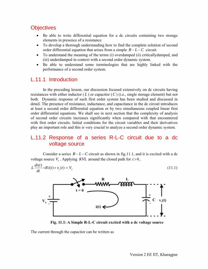
L.11.2 Response of a series R-L-C circuit due to a dc

voltage source Consider a series R L circuit as shown in fig.11.1, and it is excited with a dc voltage source

C− −sV . Applying around the closed path for , KVL 0t >

( ) ( ) ( )cdi tL R i t v tdt

+ + = sV (11.1)

The current through the capacitor can be written as


( )( ) cdv ti t Cdt

=

Substituting the current ‘ ’expression in eq.(11.1) and rearranging the terms, ( )i t2

2

( ) ( ) ( )c cc

d v t dv tsLC RC v t

dt dt+ + V= (11.2)

The above equation is a 2nd-order linear differential equation and the parameters associated with the differential equation are constant with time. The complete solution of the above differential equation has two components; the transient response and the steady state response . Mathematically, one can write the complete solution as

( )cnv t( )c fv t

( 1 21 2( ) ( ) ( ) t t

c cn c fv t v t v t A e A e Aα α= + = + +) (11.3)

Since the system is linear, the nature of steady state response is same as that of forcing function (input voltage) and it is given by a constant value . Now, the first part of the total response is completely dies out with time while and it is defined as a transient or natural response of the system. The natural or transient response (see Appendix in Lesson-10) of second order differential equation can be obtained from the homogeneous equation (i.e., from force free system) that is expressed by

A ( )cnv t0R >

2

2

( ) ( ) ( ) 0c cc

d v t dv tLC RC v tdt dt

+ + =2

2

( ) ( ) 1 ( ) 0c cc

d v t dv tR v tdt L dt LC

⇒ + + =

2

2

( ) ( ) ( ) 0c cc

d v t dv ta b c v tdt dt

+ + = (where 11, Ra b and cL L

= = =C

) (11.4)

The characteristic equation of the above homogeneous differential equation (using the

operator 2

22,d d

dt dtα α= = and ( ) 0cv t ≠ ) is given by

2 21 0 0R a b cL LC

α α α α+ + = ⇒ + + = (where 11, Ra b and cL L

= = =C

2

) (11.5)

and solving the roots of this equation (11.5) one can find the constants 1 andα α of the exponential terms that associated with transient part of the complete solution (eq.11.3) and they are given below.

2 2

1

2 2

2

1 1 ;2 2 2 2

1 12 2 2 2

R R b b acL L LC a a

R R b b acL L LC a a

α

α

⎛ ⎞ ⎛⎛ ⎞ ⎛ ⎞⎜ ⎟ ⎜= − + − = − + −⎜ ⎟ ⎜ ⎟⎜ ⎟ ⎜⎝ ⎠ ⎝ ⎠⎝ ⎠ ⎝⎛ ⎞ ⎛⎛ ⎞ ⎛ ⎞⎜ ⎟ ⎜= − − − = − − −⎜ ⎟ ⎜ ⎟⎜ ⎟ ⎜⎝ ⎠ ⎝ ⎠⎝ ⎠ ⎝

⎞⎟⎟⎠⎞⎟⎟⎠

(11.6)

where, 1Rb and cL L

= =C

.

The roots of the characteristic equation (11.5) are classified in three groups depending upon the values of the parameters , ,R L and of the circuit. C


Case-A (overdamped response): When 2 1 0

2RL LC

⎛ ⎞ − >⎜ ⎟⎝ ⎠

, this implies that the roots are

distinct with negative real parts. Under this situation, the natural or transient part of the complete solution is written as

11 2( ) t

cnv t A e A eα= + 2 tα (11.7) and each term of the above expression decays exponentially and ultimately reduces to zero as and it is termed as overdamped response of input free system. A system that is overdamped responds slowly to any change in excitation. It may be noted that the exponential term

t→∞

11

tA eα takes longer time to decay its value to zero than the term 21

tA eα . One can introduce a factor ξ that provides an information about the speed of system response and it is defined by damping ratio

( ) 122

RActual damping b Lcritical damping ac

LCξ = = = > (11.8)

Case-B ( critically damped response): When 2 1 0

2RL LC

⎛ ⎞ − =⎜ ⎟⎝ ⎠

, this implies that the roots

of eq.(11.5) are same with negative real parts. Under this situation, the form of the natural or transient part of the complete solution is written as

( )1 2( ) tcnv t A t A eα= + (where

2RL

α =− ) (11.9)

where the natural or transient response is a sum of two terms: a negative exponential and a negative exponential multiplied by a linear term. The expression (11.9) that arises from the natural solution of second order differential equation having the roots of characteristic equation are same value can be verified following the procedure given below.

The roots of this characteristic equation (11.5) are same 1 2 2RL

α α α= = = when

2 21 02 2R R 1L LC L LC

⎛ ⎞ ⎛ ⎞− = ⇒ =⎜ ⎟ ⎜ ⎟⎝ ⎠ ⎝ ⎠

and the corresponding homogeneous equation (11.4)

can be rewritten as

2

2

22

2

( ) ( ) 12 (2

( ) ( )2 (

c cc

c cc


d v t dv tor v tdt dt

α α

+ +

+ +

) 0

) 0

=

=

( ) ( )( ) ( ) 0c cc c

dv t dv tdor v t v tdt dt dt

α α α⎛ ⎞ ⎛ ⎞+ + + =⎜ ⎟ ⎜ ⎟⎝ ⎠ ⎝ ⎠

0dfor fdt

α+ = where ( ) ( )cc

dv tf v tdt

α= +


The solution of the above first order differential equation is well known and it is given by

1tf A eα=

Using the value of f in the expression ( ) ( )cc

dv tf v tdt

α= + we can get,

1 1( ) ( )( ) ( )t t tc c

c cdv t dv tv t A e e e v t A

dt dtα α αα α−+ = ⇒ + = ( ) 1( )t

cd e v t Adt

α⇒ =

Integrating the above equation in both sides yields, ( )1 2( ) t

c nv t A t A eα= +

In fact, the term 2tA eα (with

2RL

α = − ) decays exponentially with the time and tends to

zero as . On the other hand, the value of the term t→∞ 1tA t e α (with

2RL

α = − ) in

equation (11.9) first increases from its zero value to a maximum value 11

2LA eR

− at a time

1 2Lt 2LR Rα

⎛ ⎞=− = − − =⎜ ⎟⎝ ⎠

and then decays with time, finally reaches to zero. One can

easily verify above statements by adopting the concept of maximization problem of a single valued function. The second order system results the speediest response possible without any overshoot while the roots of characteristic equation (11.5) of system having the same negative real parts. The response of such a second order system is defined as a critically damped system’s response. In this case damping ratio

( ) 122


LCξ = = = = (11.10)

Case-C (underdamped response): When2 1 0

2RL LC

⎛ ⎞ − <⎜ ⎟⎝ ⎠

, this implies that the roots of

eq.(11.5) are complex conjugates and they are expressed as 2 2

1 21 1;

2 2 2 2R R R Rj j jL LC L L LC L

jα β γ α β⎛ ⎞ ⎛⎛ ⎞ ⎛ ⎞⎜ ⎟ ⎜= − + − = + = − − − = −⎜ ⎟ ⎜ ⎟⎜ ⎟ ⎜⎝ ⎠ ⎝ ⎠⎝ ⎠ ⎝

γ⎞⎟⎟⎠

. The

form of the natural or transient part of the complete solution is written as ( ) ( )1 2

1 2 1 2( ) jt tcnv t A e A e A e A e jβ γ β γα α += + = + −

= ( ) ( ) ( ) ( )1 2 1 2cos sinte A A t j A A tβ γ⎡ ⎤+ + −⎣ ⎦γ (11.11)

= ( ) ( )1 2cos sinte B t B tβ γ⎡ ⎤+⎣ ⎦γ where ( )1 1 2 2 1 2;B A A B j A A= + = −

For real system, the response must also be real. This is possible only if ( )cnv t 1 2A and A conjugates. The equation (11.11) further can be simplified in the following form:

( )sinte K tβ γ θ+ (11.12)


where β = real part of the root , γ = complex part of the root,

2 2 1 11 2

2

tan BK B B andB

θ − ⎛= + = ⎜

⎝ ⎠

⎞⎟ . Truly speaking the value of K and θ can be

calculated using the initial conditions of the circuit. The system response exhibits oscillation around the steady state value when the roots of characteristic equation are complex and results an under-damped system’s response. This oscillation will die down with time if the roots are with negative real parts. In this case the damping ratio

( ) 122


LCξ = = = < (11.13)

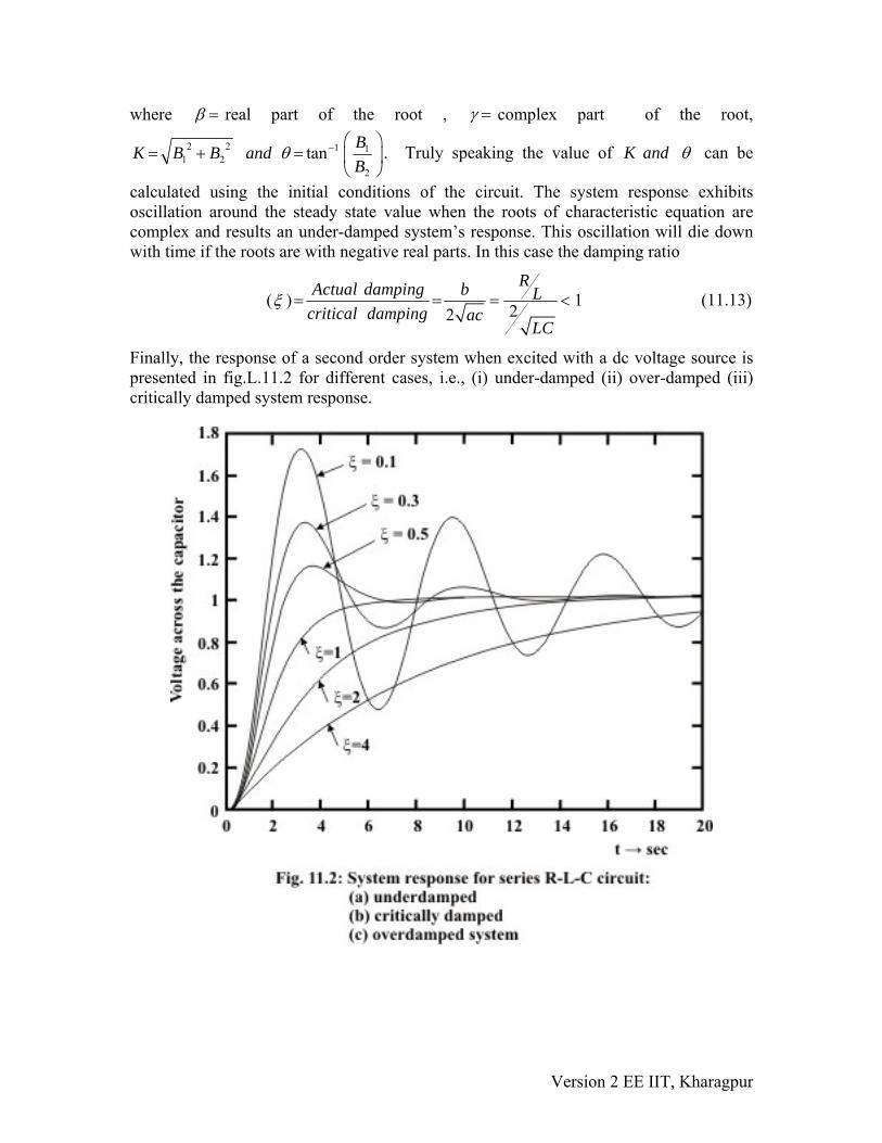
Finally, the response of a second order system when excited with a dc voltage source is presented in fig.L.11.2 for different cases, i.e., (i) under-damped (ii) over-damped (iii) critically damped system response.


Example: L.11.1 The switch was closed for a long time as shown in fig.11.3. Simultaneously at , the switch is opened and is closed Find

1S0t = 1S 2S

( ) (0 ); ( ) (0 );L ca i b v+ + ( ) (0 );Rc i + (0 )( ) (0 ); ( ) ( 0 ) ; ( ) cL c

dvd v e i fdt

++ + .

Solution: When the switch is kept in position ‘1’ for a sufficiently long time, the circuit reaches to its steady state condition. At time

1S0t −= , the capacitor is completely

charged and it acts as a open circuit. On other hand,

the inductor acts as a short circuit under steady state condition, the current in inductor can be found as

50(0 ) 6 2100 50Li A− = × =

+

Using the KCL, one can find the current through the resistor and subsequently the voltage across the capacitor

(0 ) 6 2 4Ri A− = − =(0 ) 4 50 200 .cv v− = × = olt

Note at not only the current source is removed, but 1000t += Ω resistor is shorted or removed as well. The continuity properties of inductor and capacitor do not permit the current through an inductor or the voltage across the capacitor to change instantaneously. Therefore, at the current in inductor, voltage across the capacitor, and the values of other variables at

0t +=0t += can be computed as

(0 ) (0 ) 2L Li i A+ −= = (0 ) (0 ) 200 .c c volt+ −= =; v v Since the voltage across the capacitor at 0t += is 20 , the same voltage will appear across the inductor and the 50 resistor. That is, and hence,

the current

0voltΩ (0 ) (0 ) 200 .L Rv v vo+ += = lt

( )(0 )Ri+ in resistor = 50Ω 200 4

50A= . Applying KCL at the bottom terminal


of the capacitor we obtain and subsequently, (0 ) (4 2) 6ci+ =− + =− A

(0 ) (0 ) 6 600 ./ sec.0.01

c cdv i voltdt C

+ + −= = =−

Example: L.11.2 The switch ‘ ’ is closed sufficiently long time and then it is opened at time ‘ ’ as shown in fig.11.4. Determine

S0t =

0

00

00

( ) ( )( )( ) (0 ) ( ) ( ) (0 ), ( ) ( )t

c LL

tt

dv t dv tdi ti v ii iii i and iv vdt dt dt++

+=

+ +

==

when

. 1 2 3R R= = Ω

Solution: At (just before opening the switch), the capacitor is fully charged and current flowing through it totally blocked i.e., capacitor acts as an open circuit). The voltage across the capacitor is

0t −=

(0 ) 6 (0 )c cv V v− += = = (0 )bdv + and terminal ‘b ’ is higher potential than terminal ‘ ’. On the other branch, the inductor acts as a short circuit (i.e., voltage across the inductor is zero) and the source voltage will appear across the

resistance

d6V

2R . Therefore, the current through inductor 6(0 ) 2 (0 )3L LA ii − += = = . Note at

, = 0 (since the voltage drop across the resistance 0t += (0 )adv +1 3R = Ω = )

and and this implies that = voltage across the inductor ( note, terminal ‘ c ’ is + ve terminal and inductor acts as a source of energy ).

6abv V=−

(0 ) 6cdv + = V V(0 ) 6cav + =

Now, the voltage across the terminals ‘ ’ and ‘ c ’ (b 0 (0 )v + ) = (0 ) (0 )bd cdv v+ +− = . The following expressions are valid at

0V0t +=

0 0

(0 ) 2 1 / sec.c cc

t t

dv dvC i A voltdt dt+ +

+

= =

= = ⇒ = (note, voltage across the capacitor will


decrease with time i.e., 0

1 / sec

t

dv voltdt +=

= − c ). We have just calculated the voltage

across the inductor at as 0t +=

0 0

( ) ( ) 6(0 ) 6 12 / sec.0.5

L Lca

t t

di t di tv L V Adt dt+ +

+

= =

= = ⇒ = =

Now, ( )02

(0 ) (0 ) (0 ) 1 12 3 35 / sec.c Ldv dv diR vdt dt dt

+ + +

= − = − × = − olt

Example: L.11.3 Refer to the circuit in fig.11.5(a). Determine,

(i) (ii) (0 ), (0 ) (0 )Li i and v+ + + ( )0 (0 )di dvanddt dt

+ +

(iii) ( ) ( ), Li i∞ ∞ ( )and v ∞

(assumed ) (0) 0 ; (0) 0c Lv i= =

Solution: When the switch was in ‘off’ position i.e., t < 0 - - - -

L Ci(0 ) = i (0 ) = 0, v(0 ) = 0 and v (0 ) = 0 The switch ‘ ’ was closed in position ‘1’ at time t = 0 and the corresponding circuit is shown in fig 11.5 (b).

1S

(i) From continuity property of inductor and capacitor, we can write the following expression for t = 0+

+ - + -L L c ci (0 ) = i (0 ) = 0, v (0 ) = v (0 ) = 0 1(0 ) (0 ) 0

6 ci v+ +⇒ = =

+ +Lv (0 ) = i (0 ) 6 = 0 volt× .


(ii) KCL at point ‘a’ 8 ( ) ( ) ( )c Li t i t i t= + +

At 0t += , the above expression is written as

8 (0 ) (0 ) (0 )c Li i i+ += + + + (0 ) 8ci A+⇒ =We know the current through the capacitor can be expressed as ( )ci t

cc

dv (t)i (t) = Cdt

+

+ cc

dv (0 )i (0 ) = Cdt

+

cdv (0 ) 1 = 8 × = 2 volt./sec.dt 4

∴ .

Note the relations ( )0cdv

dt

+

= change in voltage drop in 6Ω resistor = change in current through

resistor =

6Ω

6×( )0

6di

dt

+

×( )0 2

6

di

dt

+

⇒ = 1 . / sec.3

amp=

Applying KVL around the closed path ‘b-c-d-b’, we get the following expression. ( ) ( ) ( )c Lv t v t v t= +

At, the following expression 0t +=

(0 ) (0 ) (0 ) 12

(0 ) (0 )0 (0 ) 0 12 (0 ) 0 0 0

c L L

L LL L

v v i

di div v Ldt dt

+ + +

+ ++ +

= + ×

= + × ⇒ = ⇒ = ⇒ =

+

Ldi (0 ) = 0dt

and this implies +

Ldi (0 )12 = 12 0 = 0 v/secdt

× =+dv(0 ) = 0

dt


Now, at ( ) ( )Lv t R i t also= 0t += (0 ) (0 ) (0 )12 0 / sec.L Ldv di diR vdt dt dt

+ + +

= = = olt

(iii) At t α= , the circuit reached its steady state value, the capacitor will block the flow of dc current and the inductor will act as a short circuit. The current through and 12 Ω resistors can be formed as

6Ω

L12×8 16i( ) = = = 5.333A, i ( ) = 8 -5.333 = 2.667 A

18 3∞ ∞

( ) 32 .cv v∞ = olt Example: L.11.4 The switch has been closed for a sufficiently long time and then it is opened at (see fig.11.6(a)). Find the expression for (a) , (b) for inductor values of ( )

1S0t = ( )cv t ( ),ci t 0t >

0.5 ( ) 0.2i L H ii L H= = ( ) 1.0iii L H= and plot and for each case.

( )cv t vs t− −( )i t vs t− −

Solution: At (before the switch is opened) the capacitor acts as an open circuit or block the current through it but the inductor acts as short circuit. Using the properties of inductor and capacitor, one can find the current in inductor at time

0t −=

0t += as 12(0 ) (0 ) 2

1 5L Li i+ −= = =+

A (note inductor acts as a short circuit) and voltage across the

resistor = The capacitor is fully charged with the voltage across the resistor and the capacitor voltage at

5Ω 2 5 10 .volt× =5Ω 0t += is given by

(0 ) (0 ) 10 .c cv v vo+ −= = lt The circuit is opened at time 0t = and the corresponding circuit diagram is shown in fig. 11.6(b).

Case-1: 0.5 , 1 2L H R and C F= = Ω = Let us assume the current flowing through the circuit is and apply KVL equation around the closed path is

( )i t


2

2

( ) ( )( )( ) ( ) ( )c cs c s

dv t d v tdi tV R i t L v t V RC LC v tdt dt dt

= + + ⇒ = + + c (note, ( )( ) cdv ti t Cdt

= )

2

2

( ) ( ) 1 ( )c cs

d v t dv tRVdt L dt LC

= + + + cv t (11.14)

The solution of the above differential equation is given by

( ) ( ) ( )c cn cfv t v t v t= + (11.15)

The solution of natural or transient response is obtained from the force free equation or homogeneous equation which is

( )cnv t

2

2

( ) ( ) 1 ( ) 0c cc


+ + = (11.16)

The characteristic equation of the above homogeneous equation is written as

2 1 0RL LC

α α+ + = (11.17)

The roots of the characteristic equation are given as 2

11 1.0

2 2R RL L LC

α⎛ ⎞⎛ ⎞⎜ ⎟= − + − =−⎜ ⎟⎜ ⎟⎝ ⎠⎝ ⎠

; 2

21 1.0

2 2R RL L LC

α⎛ ⎞⎛ ⎞⎜ ⎟= − − − =−⎜ ⎟⎜ ⎟⎝ ⎠⎝ ⎠

and the roots are equal with negative real sign. The expression for natural response is given by

( )1 2( ) tcnv t A t A eα= + (where 1 2 1α α α= = =− ) (11.18)

The forced or the steady state response is the form of applied input voltage and it is constant ‘ ’. Now the final expression for is

( )cfv tA ( )cv t

( ) ( )1 2 1 2( ) tcv t A t A e A A t A e Aα −= + + = + +t

A

(11.19) The initial and final conditions needed to evaluate the constants are based on

(0 ) (0 ) 10 ; (0 ) (0 ) 2c c L Lv v volt i i+ − + −= = = = (Continuity property).


At ; 0t +=1 0

2 20( )c t

v t A e A A A+− ×

== + = + (11.20) 2 10A A⇒ + =

Forming ( )cdv tdt

(from eq.(11.19)as

( ) ( )1 2 1 1 2 1( ) t t tcdv t A t A e A e A t A e A e

dtα αα t− −= + + = − + +

1 2 1 20

( ) 1c

t

dv t A A A Adt +=

= − ⇒ − = (11.21)

(note, (0 ) (0 )(0 ) (0 ) 2 1 / sec.c cc L

dv dvC i i voltdt dt

+ ++ += = = ⇒ = )

It may be seen that the capacitor is fully charged with the applied voltage when and the capacitor blocks the current flowing through it. Using

t =∞t =∞ in equation (11.19) we

get, ( ) 12cv A A∞ = ⇒ =

Using the value of in equation (11.20) and then solving (11.20) and (11.21) we get, .

A1 21; 2A A=− =−

The total solution is

( ) ( )

( ) ( )

( ) 2 12 12 2 ;( )( ) 2 2 2 1

t tc

t tc

v t t e t edv ti t C t e e t e

dt

− −

− − −

=− + + = − +

⎡ ⎤= = × + − = × +⎣ ⎦t (11.22)

The circuit responses (critically damped) for 0.5L H= are shown fig.11.6 (c) and fig.11.6(d). Case-2: 0.2 , 1 2L H R and C F= = Ω = It can be noted that the initial and final conditions of the circuit are all same as in case-1 but the transient or natural response will differ. In this case the roots of characteristic equation are computed using equation (11.17), the values of roots are

1 20.563; 4.436α α=− = − The total response becomes

1 2 4.436 0.5631 2 1 2( ) t t t

cv t A e A e A A e A e Aα α − −= + + = + +t (11.23)

1 2 4.436 0.5361 1 2 2 1 2

( ) 4.435 0.563t t t tcdv t A e A e A e A edt

α αα α −= + = − − − (11.24)

Using the initial conditions( (0 ) 10cv + = , (0 ) 1 / seccdv voltdt

+

= . ) that obtained in case-1 are

used in equations (11.23)-(11.24) with 12A= ( final steady state condition) and simultaneous solution gives

1 20.032; 2.032A A= =−


The total response is

4.436 0.563

0.563 4.436

( ) 0.032 2.032 12( )( ) 2 1.14 0.14

t tc

tc

v t e edv ti t C e e

dt

− −

− −

= − +

⎡ ⎤= = −⎣ ⎦t

(11.25)

The system responses (overdamped) for 0.2L H= are presented in fig.11.6(c) and fig.11.6 (d). Case-3: 8.0 , 1 2L H R and C F= = Ω = Again the initial and final conditions will remain same and the natural response of the circuit will be decided by the roots of the characteristic equation and they are obtained from (11.17) as

1 20.063 0.243; 0.063 0.242j j j jα β γ α β γ= + = − + = − = − − The expression for the total response is

( )( ) ( ) ( ) sintc cn cfv t v t v t e K t Aβ γ θ= + = + + (11.26)

(note, the natural response ( )( ) sintcnv t e K tβ γ θ= + is written from eq.(11.12) when

roots are complex conjugates and detail derivation is given there.)

( ) (( ) sin costcdv t K e t tdt

β )β γ θ γ γ θ⎡= + +⎣ ⎤+ ⎦ (11.27)

Again the initial conditions ( (0 ) 10cv + = , (0 ) 1 / seccdv voltdt

+

= . ) that obtained in case-1 are

used in equations (11.26)-(11.27) with 12A= (final steady state condition) and simultaneous solution gives

( )04.13; 28.98 degK rθ= =− ee The total response is

( ) ( )( )

( ) (

0.063 0

0.063 0

0.063 0 0

( ) sin 12 4.13sin 0.242 28.99 12

( ) 12 4.13 sin 0.242 28.99

( )( ) 2 0.999*cos 0.242 28.99 0.26sin 0.242 28.99

t tc

tc

tc

v t e K t e t

v t e t

dv ti t C e t tdt

β γ θ −

−

−

= + + = − +

= + −

⎡ ⎤= = − − −⎣ ⎦)

(11.28)

The system responses (under-damped) for 8.0L H= are presented in fig.11.6(c) and fig. 11.6(d).



Remark: One can use in eq. 11.22 or eq. 11.25 or eq. 11.28 to verify whether it satisfies the initial and final conditions ( i.e., initial capacitor voltage

, and the steady state capacitor voltage

0t and t= =∞

olt olt(0 ) 10 .cv v+ = ( ) 12 .cv v∞ = ) of the circuit. Example: L.11.5 The switch ‘ ’ in the circuit of Fig. 11.7(a) was closed in position ‘1’ sufficiently long time and then kept in position ‘2’. Find (i) (ii) for t ≥ 0 if C

is (a)

1S( )cv t ( )ci t

19

F (b) 14

F (c) 18

F .

Solution: When the switch was in position ‘1’, the steady state current in inductor is given by

- - -L c L

30i (0 ) = = 10A, v (0 ) = i (0 ) R = 10×2 = 20 volt.1+ 2

Using the continuity property of inductor and capacitor we get + - + -

L L c ci (0 ) = i (0 ) = 10, v (0 ) = v (0 ) = 20 volt. The switch ‘ ’ is kept in position ‘2’ and corresponding circuit diagram is shown in Fig.11.7 (b)

1S

Applying KCL at the top junction point we get,

Lv (t)c + i (t) + i (t) = 0cR


Lv (t) dv (t)c c+ C + i (t) = 0

R dt

L LL

2di (t) d i (t)L + C.L + i (t) = 02R dt dt [note: ( )( ) L

cdi tv t L

dt= ]

or L LL

2d i (t) di (t)1 1+ + i (t2 RC dt LCdt) = 0 (11.29)

The roots of the characteristics equation of the above homogeneous equation can

obtained for 19

C F=

2 2

1

1 9 4×91 9+ 4 LC +RC 2 2RC 2α = =

2 2

⎛ ⎞ ⎛ ⎞− − − −⎜ ⎟ ⎜ ⎟⎝ ⎠ ⎝ ⎠ −= 1.5

2 2

2

1 9 4×91 94 LCRC 2 2RC 2α = =

2 2

⎛ ⎞ ⎛ ⎞− − − − − −⎜ ⎟ ⎜ ⎟⎝ ⎠ ⎝ ⎠ −= 3.0

Case-1 ( )1.06, over damped systemξ = : 1C = F9

, the values of roots of characteristic

equation are given as 1 21.5 , 3.0α α= − =−

The transient or neutral solution of the homogeneous equation is given by - 1.5t -3.0t

L 1 2i (t) = A e + A e (11.30)

To determine 1A and 2A , the following initial conditions are used.

At ; 0t +=+ -

L L 1

1 2

i (0 ) = i (0 ) =

102A A

A A

+

= + (11.31)

+

+ - + Lc c L

t = 0

di (t)v (0 ) = v (0 ) = v (0 ) = Ldt

- 1.5t - 3.0t120 = 2× -1.5 e -3.0 eA⎡ ⎤× ×⎣ ⎦2A (11.32)

[ ]1 2 1= 2 -1.5A -3A = - 3A - 6A2 Solving equations (11.31) and (11,32) we get , 2 116.66 , 26.666A A= − = . The natural response of the circuit is

1.5 3.0 1.5 3.0L

80 50i 26.66 16.663 3

t t te e e e− − −= − = − t−


1.5 3.0LdiL 2 26.66 1.5 16.66 3.0dt

t te e− −⎡ ⎤= ×− − ×−⎣ ⎦

( ) (

- 3.0 t - 1.5tc

- 3.0 t - 1.5t - 1.5t - 3.0t

( ) (t) = 100e - 80e

( ) 1( ) 300.0e 120e 13.33e 33.33e9

L

cc

v t v

dv ti t cdt

⎡ ⎤= ⎣ ⎦

= = − + = − )

Case-2 ( )0.707,under damped systemξ = : For 1C = F4

, the roots of the characteristic

equation are

1

2

1.0 1.01.0 1.0

j jj j

α β γα β γ

=− + = +=− − = −

The natural response becomes 1 β t

Li (t) = k e sin( t + )γ θ (11.33) Where and θ are the constants to be evaluated from initial condition. k

At , from the expression (11.33) we get, 0t +=

( )+Li 0 = k sinθ

10 = k sinθ (11.34)

+ +

β t β t

t = 0 t = 0

di(t)L = 2 k β e sin( t + ) + e cos( t + )dt

γ θ γ γ θ⎡ ⎤× ⎣ ⎦ (11.35)

Using equation (11.34) and the values of andβ γ in equation (11.35) we get, 20 2 ( cos ) cosk sn kβ θ γ θ θ= + = (note: 1, 1 sin 10and kβ γ θ= − = = ) (11.36) From equation ( 11.34 ) and ( 11.36 ) we obtain the values of θ and as k

-1 o1 1tan = = tan = 26.562 2

θ θ ⎛ ⎞⇒ ⎜ ⎟⎝ ⎠

and 10 22.36sin

kθ

= =

∴ The natural or transient solution is ( )- t o

Li (t) = 22.36 e sin t + 26.56

[ ] β tc

di(t)L = v (t) = 2 k β sin ( t +θ) + cos ( t +θ) edt

γ γ γ× ×

o o= 44.72 cos (t + 26.56 ) - sin (t + 26.56 ) te−⎡ ⎤ ×⎣ ⎦

{ o o( ) 1( ) 44.72 cos (t + 26.56 ) - sin (t + 26.56 ) e4

22.36cos( 26.56)

cc

t

dv t di t cdt dt

t e−

-t⎡ ⎤= = × ⎣ ⎦

=− +


Case-3 ( )1,critically damped systemξ = : For 1C = F8

; the roots of characteristic

equation are 1 22; 2α α=− =− respectively. The natural solution is given by ( )1 2( ) t

Li t A t A eα= + (11.37) where constants are computed using initial conditions. At ; from equation ( 11.37) one can write 0t += L 2 2i (0 ) 10A A+ = ⇒ =

( )

( )

+

+

2 1 1 0t =0

1 2 1 0

1 2 1t =0

di(t)L = 2dt

2

di(t)L (0 ) 20 2 2 30dt

t t t

t

t t

t

c

A e A t e A e

A A e A t e

v A A A

α α α

α α

α α

α α

+

+

=

=

+

⎡ ⎤× + +⎣ ⎦

⎡ ⎤= × + +⎣ ⎦

= = = − ⇒ =

The natural response is then

( ) 2( ) 10 30 tLi t t e −= +

( ) 2Ldi (t)L 2 10 30dt

td t edt

−⎡ ⎤= × +⎣ ⎦

Ldi (t)L dt

= ( )cv t [ ] 2= 2 10 60 tt e −−

( ) 2 2( ) 1( ) 2 10 60 20 308

t tcc

dv t di t c t e e t edt dt

− −⎡ ⎤ ⎡= = × × − = − +⎣ ⎦ ⎣2t− ⎤⎦

Case-4 : For ( )2,over damped systemξ = 1C =32

F

Following the procedure as given in case-1 one can obtain the expressions for (i) current in inductor (ii) voltage across the capacitor ( )Li t ( )cv t 1.08 14.93( ) 11.5 1.5t t

Li t e e− −= −14.93 1.08( ) ( ) 44.8 24.8t t

cdi tL v t e edt

− −⎡ ⎤= = −⎣ ⎦

14.93 1.08

1.08 14.93

( ) 1( ) 44.8 24.832

0.837 20.902

t tcc

t t

dv t di t c e edt dt

e e

− −

− −

⎡ ⎤= = × −⎣ ⎦

= −

L.11.3 Test your understanding (Marks: 80) T.11.1 Transient response of a second-order ------------------ dc network is the sum of two real exponentials. [1]


T.11.2 The complete response of a second order network excited from dc sources is the sum of -------- response and ---------------- response. [2]

T.11.3 Circuits containing two different classes of energy storage elements can be described by a ------------------- order differential equations. [1]

T.11.4 For the circuit in fig.11.8, find the following [6]

(0 ) (0 ) (0 ) (0 )( ) (0 ) ( ) (0 ) ( ) ( ) ( ) ( )c c L Lc c

dv dv di dia v b v c d e fdt dt dt dt

− + − +− +

(Ans. ( ) ) 6 . ( )6 . ( ) 0 / sec. ( ) 0 / sec. ( ) 0 / sec. ( ) 3 . / sec.a volt b volt c V d V e amp f amp T.11.5 In the circuit of Fig. 11.9,

Find,


(0 ) (0 )( ) (0 ) (0 ) ( ) ( ) ( ) ( )R LR L R

dv dva v and v b and c v and vdt dt

+ ++ +

L∞ ∞ [8]

(Assume the capacitor is initially uncharged and current through inductor is zero). (Ans. ( ) ) 0 , 0 ( ) 0 , 2 . / . ( )32 , 0a V V b V Volt Sec c V V

T.11.6 For the circuit shown in fig.11.10, the expression for current through inductor

is given by ( ) 2( ) 10 30 0tLi t t e for t−= + ≥

Find, ( the values of )a ,L C ( initial condition )b (0 )cv − the expression for . ( )c ( ) 0cv t >

(Ans. ( ) 21( ) 2 , ( ) (0 ) 20 ( ) ( ) 20 120 .8

tc ca L H C F b v V c v t t e V− −= = = = − ) [8]

T.11.7 The response of a series RLC circuit are given by

4.436 0.563

0.563 4.436

( ) 12 0.032 2.032

( ) 2.28 0.28

− −

− −

= + −

= −

t tc

t tL

v t e e

i t e e

where are capacitor voltage and inductor current respectively. Determine (a) the supply voltage (b) the values

( ) ( )cv t and i tL

, ,R L C of the series circuit. [4+4]

(Ans. ( ) ) 12 ( ) 1 , 0.2 2a V b R L H and C F= Ω = =

T.11.8 For the circuit shown in Fig. 11.11, the switch ‘ ’was in position ‘1’ for a long time and then at it is kept in position ‘2’.

S0t =


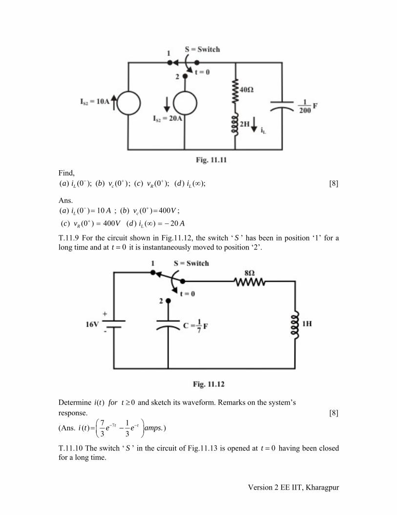
Find, ( ) (0 ); ( ) (0 ); ( ) (0 ); ( ) ( );L c R La i b v c v d i− + + ∞ [8] Ans. ( ) (0 ) 10 ; ( ) (0 ) 400 ;

( ) (0 ) 400 ( ) ( ) 20L c

R L

a i A b v V

c v V d i A

− +

+

= =

= ∞ = −

T.11.9 For the circuit shown in Fig.11.12, the switch ‘ ’ has been in position ‘1’ for a long time and at it is instantaneously moved to position ‘2’.

S0t =

Determine and sketch its waveform. Remarks on the system’s ( ) 0i t for t ≥response. [8]

(Ans. 77 1( ) .3 3

t ti t e e amps− −⎛ ⎞= −⎜ ⎟⎝ ⎠

)

T.11.10 The switch ‘ ’ in the circuit of Fig.11.13 is opened at S 0t = having been closed for a long time.


Determine (i) (ii) how long must the switch remain open for the voltage to be less than 10% ot its value at

( ) 0cv t for t ≥( )cv t 0t = ? [10]

(Ans. (i) ) ( ) 10( ) ( ) 16 240 ( ) 0.705sec.t

ci v t t e ii−= +

T.11.11 For the circuit shown in Fig.11.14, find the capacitor voltage and inductor current for all [10]

( )cv t( )Li t ( 0 0)t t and t< ≥ .

Plot the wave forms and for . ( )cv t ( )Li t 0t ≥(Ans. ( )0.5 0.5

( ) 10 sin(0.5 ); ( ) 5 cos(0.5 ) sin(0.5 )− −= = −t tc t Lv e t i t t t e )

T.11.12 For the parallel circuit shown in Fig.11.15, Find the response RLC


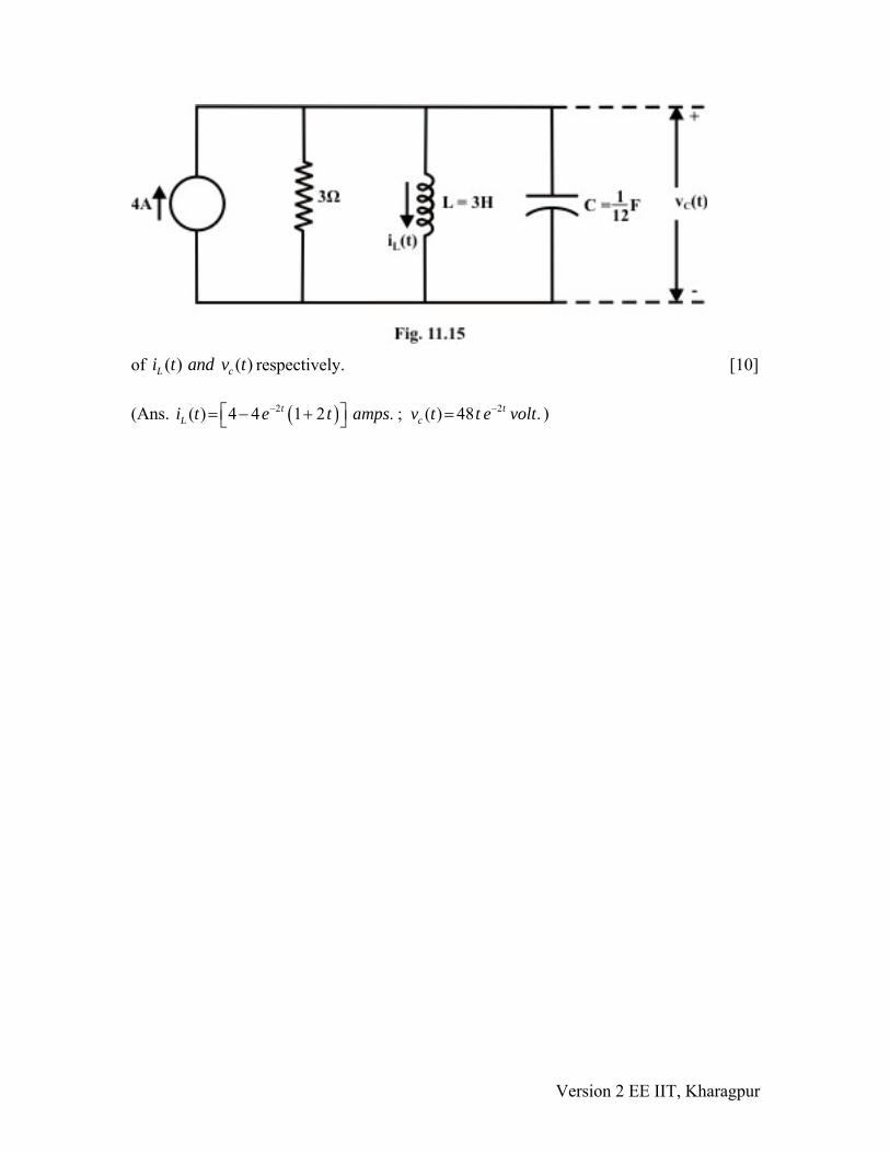
of respectively. [10] ( ) ( )Li t and v tc

(Ans. ( )2 2( ) 4 4 1 2 . ; ( ) 48 .t t

L ci t e t amps v t t e volt− −⎡ ⎤= − + =⎣ ⎦ )


Aayisha

Typewritten Text

Source:http://www.nptel.ac.in/courses/Webcourse-contents/IIT%20Kharagpur/Basic%20Electrical%20Technology/pdf/L-11(GDR)(ET)%20((EE)NPTEL).pdf

Documents

Lesson-11: Study of DC transients in circuits...Module 3 DC Transient Version 2 EE IIT, Kharagpur Lesson 11 Study of DC transients in R-L-C Circuits Version 2 EE IIT, Kharagpur Objectives