Lehrstuhl für Informatik 10 (Systemsimulation) · Lehrstuhl für Informatik 10 (Systemsimulation) Numerical Analysis of Myocardial Perfusion in the Left Ventricle by Lattice Boltzmann

FRIEDRICH-ALEXANDER-UNIVERSITÄT ERLANGEN-NÜRNBERGTECHNISCHE FAKULTÄT • DEPARTMENT INFORMATIK

Lehrstuhl für Informatik 10 (Systemsimulation)

Numerical Analysis of Myocardial Perfusion in the Left Ventricle byLattice Boltzmann Method

Sayed M. A. Al Hasnine

Master’s Thesis

Numerical Analysis of Myocardial Perfusion in the Left Ventricle byLattice Boltzmann Method

Sayed M. A. Al Hasnine

Master’s Thesis

Aufgabensteller: Prof. Dr. U. Rüde

Betreuer: Dipl.-Inform. C. Godenschwager

Bearbeitungszeitraum: 09.7.2013 – 08.01.2014

Erklärung:

Ich versichere, dass ich die Arbeit ohne fremde Hilfe und ohne Benutzung andererals der angegebenen Quellen angefertigt habe und dass die Arbeit in gleicher oderähnlicher Form noch keiner anderen Prüfungsbehörde vorgelegen hat und von dieserals Teil einer Prüfungsleistung angenommen wurde. Alle Ausführungen, die wörtlichoder sinngemäß übernommen wurden, sind als solche gekennzeichnet.

Erlangen, den 8. Januar 2014 . . . . . . . . . . . . . . . . . . . . . . . . . . . . . . . . .

4

5

Abstract

Cardiovascular diseases are identified as the major cause of death worldwide. Thesuccessful treatment depends largly on an accurate analysis of the hemodynamical im-pact of cardiovascular pathophysiology. An active research is going on to understandthe dynamics of the heart and it’s vasculature, also; the computational approach isgaining acceptance as a useful tool to simulate the blood flow in the vessels. Differentmodels and numerical schemes (e.g. finite element) have been followed to simulate theblood flow in vessels and myocardium so far.

During the last decade, the Lattice Boltzmann Method has reached to a level, whereit can be considered an alternative to available continuum based numerical methods inmost fluid related problems. The method is based on kinetic theory and can be usedto derive the Navier-Stokes equations in small knudsen number limit. It has attractiveoption of local and highly scalable parallel computation. The theories of this methodis revisited and reviewed in details.

In this thesis, a method with a porous medium model of Lattice Boltzmann Methodis presented to simulate the myocardial perfusion in the left ventricle of the patient spe-cific geometries. The computer code is also tested for some well known fluid dynamicsproblems and compared with available literature data.

6

7

Acknowledgements

I would like to take this opportunity to acknowledge some people for their help andsupport, without which this thesis wouldn’t be possible.

I would like to express my profound gratitude to Prof. Dr. Ulrich Rüde and Chris-tian Godenschwager for acting as supervisors and giving me the chance to work onthis interesting project. Special thanks to Christian Godenschwager for guiding mefrom the beginning, answering all of my questions with patience; no matter how pettythey were, introducing me to the professional coding, sometimes giving me freedom toexplore on my own and most of all creating an active environment for finishing thisthesis. I would also like to thank Frank Deserno for helping me with the computers atthe CIP-Pool from time to time.

I am grateful to the COSSE consortium for giving me the opportunity to spendtwo amazing academic years for my Masters study. It helped me to learn and enhancemy knowledge of the numerical mathematics and computational fluid dynamics. Mysincere thanks to the program co-ordinator Dr. Michael Hanke at KTH, Sweden andDr. Harald Köstler at FAU, Germany for guiding me with the courseworks and KarinKnutsson at KTH, Sweden for making my life easy by helping me with the adminis-trative works during my stay at these universities.

I am thankful to the colleagues at the SIEMENS Healthcare, Forchheim for ac-cepting me as a part of the team and maintaining a good working environment.

And my dearest parents, who always supported me and encouraged me in my en-deavour.

8

9

Contents

Abstract 5

Acknowledgements 7

List of Figures 11

List of Tables 14

1 Introduction 151.1 Motivation . . . . . . . . . . . . . . . . . . . . . . . . . . . . . . . . . . 151.2 Current Developments and Methodologies . . . . . . . . . . . . . . . . 161.3 Objectives and Structure of the Thesis . . . . . . . . . . . . . . . . . . 17

2 Theoretical Background 192.1 Cardiovascular System . . . . . . . . . . . . . . . . . . . . . . . . . . . 19

2.1.1 Physics of the Heart . . . . . . . . . . . . . . . . . . . . . . . . 202.1.2 The Heart Wall (Myocardium) . . . . . . . . . . . . . . . . . . . 232.1.3 Coronary Circulation . . . . . . . . . . . . . . . . . . . . . . . . 24

2.2 Hemodynamics . . . . . . . . . . . . . . . . . . . . . . . . . . . . . . . 262.2.1 Viscosity . . . . . . . . . . . . . . . . . . . . . . . . . . . . . . . 262.2.2 Rheology of the Blood . . . . . . . . . . . . . . . . . . . . . . . 272.2.3 Resistance . . . . . . . . . . . . . . . . . . . . . . . . . . . . . . 29

2.3 Flow through Porous Medium . . . . . . . . . . . . . . . . . . . . . . . 302.3.1 Darcy’s law . . . . . . . . . . . . . . . . . . . . . . . . . . . . . 302.3.2 Brinkman’s Extension . . . . . . . . . . . . . . . . . . . . . . . 322.3.3 Forchheimer’s Extension . . . . . . . . . . . . . . . . . . . . . . 322.3.4 Generalized Model . . . . . . . . . . . . . . . . . . . . . . . . . 322.3.5 Pre Darcy, Darcy and Non Darcy Flow . . . . . . . . . . . . . . 34

3 Numerical Approach of the Problem 353.1 The Lattice Boltzmann Method (LBM) . . . . . . . . . . . . . . . . . . 35

3.1.1 Continuum and Discrete Approach . . . . . . . . . . . . . . . . 363.1.2 Boltzmann - Maxwell Equations . . . . . . . . . . . . . . . . . . 363.1.3 Discrete Lattice Boltzmann Equation (LBE) . . . . . . . . . . . 393.1.4 LBE to NSE . . . . . . . . . . . . . . . . . . . . . . . . . . . . . 42

3.2 Boundary Conditions for LBM . . . . . . . . . . . . . . . . . . . . . . . 433.2.1 Bounce-back Boundary Condition . . . . . . . . . . . . . . . . . 443.2.2 Free-Slip Boundary Condition . . . . . . . . . . . . . . . . . . . 45

10 CONTENTS

3.2.3 Periodic Boundary Condition . . . . . . . . . . . . . . . . . . . 453.2.4 Velocity Bounce-back Boundary Condition . . . . . . . . . . . . 463.2.5 Simple Pressure Anti Bounce-back Boundary Condition . . . . . 46

3.3 Physical to Lattice System . . . . . . . . . . . . . . . . . . . . . . . . . 473.4 LBM Models for Porous Medium Flows . . . . . . . . . . . . . . . . . . 48

3.4.1 Generalized LBM Model for Porous Medium Flows . . . . . . . 493.5 The waLBerla Framework . . . . . . . . . . . . . . . . . . . . . . . . . 50

4 Simulation and Comparison with Literature Data 514.1 Lid Driven Cavity Flow . . . . . . . . . . . . . . . . . . . . . . . . . . 514.2 Couette Flow . . . . . . . . . . . . . . . . . . . . . . . . . . . . . . . . 554.3 Method for Simulating the Myocardial Perfusion . . . . . . . . . . . . . 58

5 The 3D Perfusion Model 615.1 Geometries . . . . . . . . . . . . . . . . . . . . . . . . . . . . . . . . . 615.2 Boundary Conditions and Setup . . . . . . . . . . . . . . . . . . . . . . 645.3 Simulations and Results . . . . . . . . . . . . . . . . . . . . . . . . . . 70

6 Summary 73

7 Conclusion 75

8 References 77

11

List of Figures

1.1 The steps of surgical procedure for stent placement. [5] . . . . . . . . . 15

1.2 Flow chart of patient specific simulation for predictive medicine. (mod-ified and reproduced from [6]) . . . . . . . . . . . . . . . . . . . . . . . 17

2.1 Blood circulation in human heart. The blue color represents the deoxy-genated blood and red color represents the oxygenated blood supply.(modified from Wikimedia Commons) . . . . . . . . . . . . . . . . . . . 20

2.2 Blood circulatory system from heart towards body and lungs, the par-allel arrangement except the liver circulation where blood flows fromgastrointestinal (GI) as well as from the branch of aorta. The red colorrepresents the vessels carrying oxygenated blood, e.g. arteries and theblue color represents the vessels carrying deoxygenated blood, e.g. veins.(reproduced from [12]) . . . . . . . . . . . . . . . . . . . . . . . . . . . 21

2.3 Structure of heart with pressure specifications.(reproduced from [13]) . 22

2.4 Cardiac cycle; 1- atrial systole; 2- isovolumetric contraction; 3- rapidejection; 4- reduced ejection; 5- isovolumetric relaxation; 6- rapid fill-ing; and 7- reduced filling. Sys(systole); Dias(diastole); AP(aortic pres-sure); LVP(left ventricular pressure); LAP(left atrial pressure); LV( leftventricle); LVEDV (left ventricular end-diastolic volume); LVESV(leftventricular end-systolic volume). (reproduced from [12]) . . . . . . . . 22

2.5 The heart wall. (wikipedia) . . . . . . . . . . . . . . . . . . . . . . . . 23

2.6 Detailed anterior and posterior views of Coronary Circulation. LAD:left anterior descending coronary artery AIV: anterior interventricularvein CFX: circumflex coronary artery RCA: right coronary artery GCV:great cardiac vein PDA: posterior descending artery CS: coronary sinusMCV: middle cardiac vein SCV: small cardiac vein. (reproduced from[21]) . . . . . . . . . . . . . . . . . . . . . . . . . . . . . . . . . . . . . 23

2.7 Circulatory arrangement of major blood vessels. (reproduced from [12]) 24

2.8 Square root of shear stress vs square root of shear strain rate in typicalhuman blood. (reproduced from [27]) . . . . . . . . . . . . . . . . . . . 27

2.9 Relative viscosity (ratio of apparent viscosity to plasma viscosity) vsdiameter of the vessel. (reproduced from [22]) . . . . . . . . . . . . . . 28

2.10 The relative size of different scales. (reproduced from [16]) . . . . . . . 30

2.11 Specifications for Darcy’s law. . . . . . . . . . . . . . . . . . . . . . . . 31

2.12 flow zones in porous medium as a function of pressure gradient. Super-ficial velocity is the volumetric flow per unit surface area. (reproducedfrom [48]) . . . . . . . . . . . . . . . . . . . . . . . . . . . . . . . . . . 34

12 LIST OF FIGURES

3.1 Different approaches of simulation. (reproduced from [56]) . . . . . . . 37

3.2 Illustration of the collision and streaming steps. . . . . . . . . . . . . . 39

3.3 Single lattice cell for two (D2Q9) and three (D3Q19) dimensional sim-ulation. . . . . . . . . . . . . . . . . . . . . . . . . . . . . . . . . . . . 40

3.4 Illustration of the bounce back boundary condition for On-grid approach(D2Q9). The dashed green line represents the bounce back of distribu-tion functions, solid brown line represents the streaming and the solidblue line represents the post collision scheme. (reproduced from [59]) . 44

3.5 Illustration of the bounce back boundary condition for Mid-grid ap-proach (D2Q9). The dashed green line represents the bounce back ofdistribution functions, solid brown line represents the streaming and thesolid blue line represents the post collision scheme. (reproduced from[59]) . . . . . . . . . . . . . . . . . . . . . . . . . . . . . . . . . . . . . 45

3.6 Illustration of the periodic boundary condition along x direction in twodimension (D2Q9). . . . . . . . . . . . . . . . . . . . . . . . . . . . . . 46

4.1 Velocity profile of the x component of the velocity along the verticalline for different Darcy numbers for Re = 10 and ǫ = 0.1 for lid drivencavity flow. . . . . . . . . . . . . . . . . . . . . . . . . . . . . . . . . . 52

4.2 Velocity profile of the y component of the velocity along the horizontalline for different Darcy numbers for Re = 10 and ǫ = 0.1for lid drivencavity flow. . . . . . . . . . . . . . . . . . . . . . . . . . . . . . . . . . 52

4.3 Simulation results for Da=10−4for lid driven cavity flow. ∆x = 1 and∆t = 1. . . . . . . . . . . . . . . . . . . . . . . . . . . . . . . . . . . . 53

4.4 Simulation results for Da=10−3 for lid driven cavity flow. ∆x = 1 and∆t = 1. . . . . . . . . . . . . . . . . . . . . . . . . . . . . . . . . . . . 53

4.5 Simulation results for Da=10−2 for lid driven cavity flow. ∆x = 1 and∆t = 1. . . . . . . . . . . . . . . . . . . . . . . . . . . . . . . . . . . . 54

4.6 Velocity profile of the x component of the velocity along the verticalline for different Darcy numbers for Re = 10 and ǫ = 0.1 for couette flow. 55

4.7 Velocity profile of the x component of the velocity along the vertical linefor different Reynolds numbers for Da = 0.01 and ǫ = 0.1 for couetteflow. . . . . . . . . . . . . . . . . . . . . . . . . . . . . . . . . . . . . . 56

4.8 Velocity profile of the x component of the velocity along the verticalline for Re = 0.01 and Da = 0.001 for couette flow considering porosityǫ = 0.1 in the bottom half domain. . . . . . . . . . . . . . . . . . . . . 56

4.9 Velocity magnitude in pseudocolor for Da = 1e − 02, Re = 10 andǫ = 0.1 for full porous medium couette flow. ∆x = 1 and ∆t = 1. . . . 57



4.12 The setup of the problem. Red color stands for the no slip conditionand blue is the fluid or porous region. . . . . . . . . . . . . . . . . . . . 58

4.13 Porosity field in the domain. . . . . . . . . . . . . . . . . . . . . . . . . 59

4.14 Velocity field in the domain. . . . . . . . . . . . . . . . . . . . . . . . . 59

LIST OF FIGURES 13

5.1 Geometry of the left coronary artery with inflow and outflow tagged bydifferent colors of the first patient. The red color represents inflow andthe blue color represents the outflow boundary of the geometry. . . . . 62

5.2 The geometries from the first patient. . . . . . . . . . . . . . . . . . . . 625.3 Geometry of the left coronary artery with inflow and outflow tagged by

different colors of the second patient. The red color represents inflowand the blue color represents the outflow boundary of the geometry. . . 63

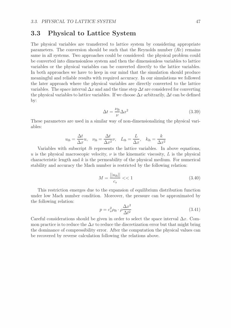
5.4 The geometries from the second patient. . . . . . . . . . . . . . . . . . 635.5 The setup and structured mesh of GEOM1. . . . . . . . . . . . . . . . 665.6 Clipped portion of the structured mesh and boundary conditions of

GEOM1. . . . . . . . . . . . . . . . . . . . . . . . . . . . . . . . . . . . 675.7 The setup and structured mesh of GEOM2. . . . . . . . . . . . . . . . 685.8 Clipped portion of the structured mesh and boundary conditions of

GEOM2. . . . . . . . . . . . . . . . . . . . . . . . . . . . . . . . . . . . 695.9 Velocity field (lattice unit) in pseudocolor after 75 × 103 time steps in

GEOM1, full domain (left) and clipped domain (right). ∆x = 4e− 4cm. 715.10 Pressure field (lattice unit) in pseudocolor after 75 × 103 time steps in

GEOM1, full domain (left) and clipped domain (right). ∆x = 4e− 4cm. 715.11 Velocity field (lattice unit) in pseudocolor after 75 × 103 time steps in

GEOM2, full domain (left) and clipped domain (right). ∆x = 3e− 4cm. 725.12 Pressure field (lattice unit) in pseudocolor after 75 × 103 time steps in

GEOM2, full domain (left) and clipped domain (right). ∆x = 3e− 4cm. 72

14

List of Tables

2.1 Internal Diameter and wall thickness of the blood vessels. (reproducedfrom [39]) . . . . . . . . . . . . . . . . . . . . . . . . . . . . . . . . . . 25

2.2 Properties of various blood cells. (reproduced from [23]) . . . . . . . . 28

3.1 Magnitude of velocity bits and weighting factors for different latticemodels. (reproduced from [54]) . . . . . . . . . . . . . . . . . . . . . . 40

15

Chapter 1

Introduction

1.1 Motivation

According to the World Health Organization (WHO), cardiovascular diseases (CVDs)are the main cause of death around the world [1]. These are caused by the diseasedarteries; that supply blood to the brain, heart’s wall, legs or arms and the diseasedheart muscle or the diseased heart valves. It can be congenital or acute. Atherosclero-sis is the most common among the CVDs which involves deposition or accumulationof fatty objects in the form of plaque in the innermost layer of the artery wall [2]. Thisobstructs the blood flow to the respective organs, hampering the supply of oxygenand other necessary nutrients to the cells of these organs. The formation or site ofatherosclerotic lesions are not random, they are localized and maintain a pattern [3].DeBakey et al. [4] identified five predominent sites for plaque formation: the coro-nary artery, the major branches of the aortic arch, the visceral arterial branches ofthe abdominal aorta, the terminal abdominal aorta as well as its major branches andcombination of these two or more sites.

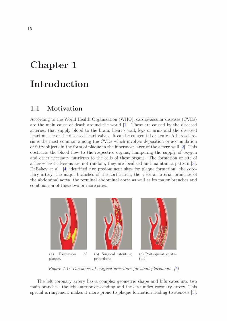
(a) Formation ofplaque.

(b) Surgical stentingprocedure.

(c) Post-operative sta-tus.

Figure 1.1: The steps of surgical procedure for stent placement. [5]

The left coronary artery has a complex geometric shape and bifurcates into twomain branches: the left anterior descending and the circumflex coronary artery. Thisspecial arrangement makes it more prone to plaque formation leading to stenosis [3].

16 CHAPTER 1. INTRODUCTION

The more susceptible zones are the outer walls of the bifurcation and least affectedareas are the walls of the divider of the blood flow as well as the inner walls far from thebifurcation zone [3]. It is assumed that a complex relation between the hemodynamicforces (e.g. shear stress, cyclic circumferential strain) and the biochemical activityfacilitate the formation of plaque in these regions [3]. Stenosis can also form due tounusual narrowing of the wall of blood vessels instead of plaque formation inside thevessel. This kind of lesions can lead to ischemia or myocardial infarction, in generalheart attack; due to malperfused myocardial sites. One of the current surgical prac-tices is to place a stent inside the blood vessel where the stenosis is formed by meansof a catheter and dilating it. The steps of the treatment are shown in Figure 1.1.Coronary artery bypass surgery is another way of treating the stenosis by ensuring adifferent pathway for blood flow to the myocardium.

Information on perfusion in the heart can be very useful to determine the state andcondition of the heart. Several invasive and non-invasive methods are used to gatherthe information, e.g. electrocardiography (ECG), coronary angiography, echocardio-gram etc. However, surgical planning, medical device design and medical researchdemand more data for the prediction of the treatment. Computational tools can helpto get the insight of the CVDs. Blood flow simulation in the original geometry canprovide valuable information regarding the pressure, flow rate as well as perfusion inthe heart. The heart wall (myocardium) can be considered as porous medium for thesimulation purpose [18].

1.2 Current Developments and Methodologies

The conventional procedure for surgical planning for the patients suffering from pos-sible CVDs, is based on invasive measurements, medical imaging data as well as em-pirical data on treating similar cases and the success of the treatment greatly dependson how well the physicians can predict the status of the patients [6]. However, thehuman physiology varies from person to person and hence, the data acquired by theconventional method might not be enough to reach to a conclusion on procedures andpredicting the result of such procedures for the treatment. Charles et al. [6] presenteda new model of predictive medicine. This is a Computational Fluid Dynamics (CFD)based patient specific model to simulate the blood flow. The physcian can construct amodel of the patient using the proper diagnostic data and simulate the post-treatmentstatus of the patient in different physiological conditions. The model adopts the fi-nite element method for the simulation. The geometries are derived from ComputedTomography (CT ) or Magnetic Resonance Imaging (MRI) technique. The boundaryconditions are determined according to the patient specific diagnostic data. In general,the simulation based medical planning procedure could be represented in a flow chart,depicted in Figure 1.2.

Westerhof et al. [7] studied and reviewed the cross-talk between cardiac muscle andcoronary vasculature. They concluded that, the coronary flow is hindered or reversedduring the systolic phase but in diastole the effect of cardiac muscle on coronary flowis small. However, the perfusion pressure increases the stiffness of the ventricle during

1.3. OBJECTIVES AND STRUCTURE OF THE THESIS 17

Figure 1.2: Flow chart of patient specific simulation for predictive medicine. (modifiedand reproduced from [6])

diastole. They also discussed different models (e.g. waterfall model, intramyocar-dial pump model, varying elastance model etc.) and their limitations for explainingthe relation between the cardiac muscle and the coronary vasculature. Huyghe et al.[8] presented a porous medium finite element model for the diastolic left ventricle.This model considers the fiber orientation in the myocardium. They considered themyocardium as a two phase mixture of solid and liquid. The flow of liquid followsthe Darcy’s law. This model also allows to consider the anisotropy of permeability.Cookson et al. [9] presented a poroelastic, incompressible finite element model for my-ocardial perfusion. The model divides the fluid phase into multicomponent pore spaceaccording to vascular groups. Thus it introduces the flexibility of defining differentpermeability for different compartments.

1.3 Objectives and Structure of the Thesis

The objective of this thesis is to present a primary model for simulating the myocardialperfusion in the left ventricle. An attempt is taken for the first time to simulate themyocardial perfusion by the Lattice Boltzmann Method (LBM). Patient specific ge-ometries are considered for the simulations. The thesis can be divided into two parts.In the first part physiological aspects of the heart, blood, vasculature and theory ofLBM is studied and reviewed. The second part discusses the ability of the code, used

18 CHAPTER 1. INTRODUCTION

for the perfusion simulation; to reproduce the literature data and the model to sim-ulate the myocardial perfusion. The flexibility of the Lattice Boltzmann Method hasbeen exploited to use patient specific geometries in the following study.

Chapter 2 provides theoretical background of the cardiovascular system, hemo-dynamical issues related to the blood and the porous medium flow. The aim of thischapter is to provide a complete picture of problem and the available theories to dealwith that.

Chapter 3 discusses the details of the numerical method (LBM) followed to sim-ulate the myocardial perfusion. Boundary conditions for the LBM is discussed in aseparate section. The summary of the code structure is also given for the interestedreaders.

Chapter 4 presents the simulation results for lid driven cavity flow and couetteflow with the present code and comparison with the literature data. The method thatis followed to simulate the myocardial perfusion, is discussed with an example in aseparate section.

Chapter 5 presents the three dimensional model for the myocardial perfusion. Thegeometries of two different patients are presented. Boundary conditions and setup ofthe model is discussed. Finally, the simulated results are presented.

Chapter 6 discusses the theories, which was followed to develop the method tosimulate the myocardial perfusion. The simulation results were also discussed.

Chapter 7 is the concluding chapter. It summarizes the procedures and findingsof the work. A direction of the future works is also presented.

19

Chapter 2

Theoretical Background

2.1 Cardiovascular System

The living cells need oxygen and other nutrients (e.g. glucose, amino acids) to continuetheir function properly and a system to remove the by products of their activity (e.g.carbon di oxide, lactic acid). Moreover, the cells belonging to the inner organs of thebody need a convection-diffusion circulatory system to ensure this mechanism [10,11].In case of most of the mammals, this problem is taken care by the blood circulationsystem in arteries, veins and their capillaries. Blood acts as a medium to transportthe neccessary elements for the cells by convection as well as collecting the waste ofthe cells by diffusion process.

The main components of the cardiovascular system are the heart, the blood vesselsand the blood. The heart maintains the circulation of blood in different organs. Theblood circulation can be divided into two main parts, the systemic circulation (SC)and the pulmonary circulation (PC). The PC is the circulation of blood between theheart and the lungs. The exchange of oxygen and carbon dioxide takes place betweenblood in the pulmonary capillaries and the lung alveoli. SC is the circulation of bloodbetween the organs other than the lungs and the heart.

The deoxygenated blood flows from superior vena cava (SVC) and inferior venacava (IVC) to right atrium (RA) then to right ventricle (RV) through tricuspid valve.The right ventricle pumps the blood to the lungs through pulmonary artery; passingpulmonary valve (PV). The oxygenated blood is carried by the pulmonary veins toleft atrium (LA) from the lungs, which pumps the blood to left ventricle (LV) throughmitral valve. The blood from LV enters the aorta through the aortic valve (AV). Allthese valves act as one way valves, blood is allowed to pass only in one direction.The LV pumps blood towards the body through aorta and to the heart muscle itselfthrough coronary artery. In our study we have only considered SC. Mean pressure inthe SC is about 97.51 mmHg (13 KPa) and in PC is about 30 mmHg (4 KPa) [11].The circulation is illustrated in Figure 2.1.

Again, the arrangement of the cardiovascular system can be divided into seriessystem and parallel system as shown in Figure 2.2. SC and PC can be identified asoperating in series systems. The amount of blood that enters the PC from RV , also

20 CHAPTER 2. THEORETICAL BACKGROUND

Figure 2.1: Blood circulation in human heart. The blue color represents the deoxy-genated blood and red color represents the oxygenated blood supply. (modified fromWikimedia Commons)

enters the SC from LV . So, the output of both sides of the heart nearly matches eachother. Moreover, the blood passing through the organs are in parallel arrangement asshown in Figure 2.2.

2.1.1 Physics of the Heart

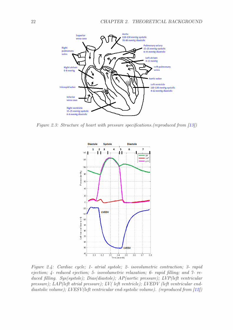
The heart is a complicated fluid pump. It operates in a closed system, provides nour-ishments for itself. It has four chambers, namely: right and left atrium, right and leftventricle as discussed before. These chambers are separated by interatrial and inter-ventricular septum. The wall of the left ventricle is thicker than the right ventriclebecause the left one has to work in a high pressure environment, Figure 2.3.

The heart undergoes subsequent ventricular contraction (systole) and relaxation(diastole) to pump the blood from high pressure arterial system to low pressure venoussystem. However, the cardiac cycle has seven phases [12], atrial systole, isovolumetriccontraction, rapid ejection, reduced ejection, isovolumetric relaxation, rapid filling andreduced filling. The illustration of the phases for the left side (LV and LA) has been

2.1. CARDIOVASCULAR SYSTEM 21

Figure 2.2: Blood circulatory system from heart towards body and lungs, the parallelarrangement except the liver circulation where blood flows from gastrointestinal (GI)as well as from the branch of aorta. The red color represents the vessels carryingoxygenated blood, e.g. arteries and the blue color represents the vessels carrying de-oxygenated blood, e.g. veins. (reproduced from [12])

given in Figure 2.4. In the atrial systolic phase, the atrium contracts, mitral valveopens and aortic valve closes, blood flows from the LA to the LV. However, most ofthe filling of the LV happens before this phase. The next phase is the isovolumetriccontraction, the volume of the blood remains constant as all the valves are closed. Thepressure at the LV increases rapidly. Rapid ejection phase is the phase when the aorticvalve opens and the mitral valve remains closed, the pressure inside the LV exceedsthat of the aorta as the LV contracts. The flow of blood from LV through aorta occursdue to the pressure gradient. Soon after that, the muscle of the LV starts to relax andthe reduced ejection phase starts. The pressure in the LV decreases. This is the endphase of systole. As the pressure is decreasing in the LV, at a certain point of time thetotal energy (pressure energy and kinetic energy) within the LV becomes less than inthe LA. All the valves are closed and the isovolumetric relaxation phase begins. Thisis the first phase of diastole. The next phase of diastole is the rapid filling. Mitralvalve opens and the aortic valve closes. The volume of the LV reaches it’s maximumstate just before the mitral valve opens, causing rapid filling of the LV. As the LV isfilling and expanding the pressure rises and this causes the flow of blood from the LAto the LV reduced.


Figure 2.3: Structure of heart with pressure specifications.(reproduced from [13])

Figure 2.4: Cardiac cycle; 1- atrial systole; 2- isovolumetric contraction; 3- rapidejection; 4- reduced ejection; 5- isovolumetric relaxation; 6- rapid filling; and 7- re-duced filling. Sys(systole); Dias(diastole); AP(aortic pressure); LVP(left ventricularpressure); LAP(left atrial pressure); LV( left ventricle); LVEDV (left ventricular end-diastolic volume); LVESV(left ventricular end-systolic volume). (reproduced from [12])


(a) Layers of the heart wall (b) Muscle tissue viewed underthe microscope

Figure 2.5: The heart wall. (wikipedia)

2.1.2 The Heart Wall (Myocardium)

The wall of heart is mainly composed of three layers, Figure 2.5. The endocardium isthe interior layer of the heart which is smooth for carrying the blood in the chamber.The myocardium is the middle layer, thickest heart muscle which pumps the bloodfrom ventricle towards body and lung. It contracts during systole and relaxes duringdiastole. The muscle cells have one nucleus and operate independently. However, theyare connected through intercalated disks, which pass electric impulses and synchronizethe systolic and diastolic phases, Figure 2.5 . The epicardium is the outer-most layerwhich shapes the heart.

Figure 2.6: Detailed anterior and posterior views of Coronary Circulation. LAD: leftanterior descending coronary artery AIV: anterior interventricular vein CFX: cir-cumflex coronary artery RCA: right coronary artery GCV: great cardiac vein PDA:posterior descending artery CS: coronary sinus MCV: middle cardiac vein SCV: smallcardiac vein. (reproduced from [21])


2.1.3 Coronary Circulation

The heart is a vital organ and the system which helps it to continue it’s functionality,is the coronary circulation. This system is composed of coronary arteries that carrythe oxygen rich blood to the myocardium and supply it with oxygen and necessarynutrients. Coronary veins carry the blood out of the myocardium. The main two coro-nary arteries are the left and right coronary arteries which are branched off to smallarteries and arterioles, capillaries. The right coronary artery perfuses blood to rightatrium and ventricle. On the other hand, the left coronary artery branches into leftanterior descending artery, and the left circumflex artery. The left circumflex artery issurrounded by myocardial tissue inside the septum. The left coronary artery mainlysupplies blood to the left ventricle and left atrium. Other large arteries supply bloodto the epicardial surface of the heart and therefore are referred to as epicardial arteries[18].

Figure 2.7: Circulatory arrangement of major blood vessels. (reproduced from [12])

The larger coronary arteries run through the epicardial surface of the heart. Thesearteries branch into smaller arteries, arterioles and capillaries that enter the my-ocardium. The branch consists of many capillary networks, serving blood nutrients tothe muscle cells (myocytes).

The blood from the branches of the coronary arteries then enter the cardiac veinsystem. The system can be divided into three major vein systems [19]: tributaries ofthe coronary sinus, anterior cardiac veins and atrial cardiac veins. The major veinsjoin together to form the coronary sinus, which collectes the deoxygenated blood fromthe heart muscle. The great cardiac vein (GCV), largest among the tributaries ofcoronary sinus, starts from the apex of heart and carries the deoxygenated blood tothe coronary sinus. It collects blood from the left side of the heart (left coronary andleft atrium). The anterior interventricular vein (AIV) is a tributary of the GCV andsituated in parallel with the left anterior descending coronary artery. It receives bloodfrom the left ventricular branches. The middle cardiac vein starts from the apex of theheart and runs through the posterior interventricular sulcus towards coronary sinus.


Posterior interventricular sulcus is the groove which separates the right ventricle fromthe left ventricle. The small cardiac vein also opens into coronary sinus. The coronarysinus accounts for approximately 85% of the venous drainage [20] to the right atrium.It drains the left ventricle, some part of the right ventricle, both atria and anteriorportion of the interventricular septum. The second system of anterior cardiac veinsaren’t connected to the coronary sinus. These veins carry deoxygenated blood fromthe anterior right ventricular wall and enter the right atrium. The third system ofatrial cardiac veins generally drain into the coronary sinus but sometimes it has beenfound to carry the deoxygenated blood directly to the right atrium.

Vessel Diameter Wall ThicknessAorta 25mm 2mmArtery 4mm 1mm

Arteriole 30µm 6µmTerminal Arteriole 10µm 2µm

Capillary 8µm 0.5µmVenule 20µm 1µmVein 5mm 0.5mm

Vena Cava 30mm 1.5mm

Table 2.1: Internal Diameter and wall thickness of the blood vessels. (reproduced from[39])

As the diameter of the blood vessel decreases, the thickness of the wall also de-creases. The wall of capillaries are only one cell thick [22]. Thus it is ideal for theexchange of substances between blood and tissue. The arrangement has been illus-trated in Figure 2.7. The inner diameter and the thickness of the vessel wall are givenin Table 2.9.


2.2 Hemodynamics

Hemodynamics is the study of blood flow through vessels and the factors affecting theflow. The blood flow is mainly determined by these two factors, pressure differenceand resistance. If we consider the Poiseuille flow (originally used to describe the flowdue to pressure drop through a long cylindrical pipe), a relationship can be establishedamong the pressure drop, resistance and flow. From Nasimi [14], volumetric flow rateis given by:

Q =∆P

R(2.1)

Q is the volumetric flow rate (m3/s), ∆P is the pressure difference between two endsof the vessel (N/m2), R is the resistance to the flow and can be defined as, R = 8µL

πr4.

r is the radius of the vassel (m), µ is the dynamic viscosity (Pa.s) of the fluid, and Lis the length of the vessel (m). This relation also resembles the Darcy’s law which willbe discussed in the later part of this report.

R is proportional to the L, but as L remains constant for blood circulation; theeffect of L remains unchanged. However, R is inversly proportional to the fourth powerof r. Thus, r has greater effect on the flow as a small change of r can change the flowfield entirely. r is not constant along the length of the blood vessels, as the value ofr decreases the flow reduces due to increase of the resistance. The main resistance islocated at the arterioles (the reason for the capillaries not being the major resistivevessels, is discussed in section 2.2.3). The total resistance of arterioles is about 100times as large as the resistance of aorta [14]. Moreover, sudden change of the radiuscan trigger the instability leading to turbulence. In that case, the Poiseuille Equation(2.1) is not valid anymore. Aortic stenosis is an ideal example of such situation.

2.2.1 Viscosity

Dynamic viscosity (µ,Pa · s) or viscosity in general, is the fluid property which mea-sures the fluid’s resistance to flow. It is a constant property for Newtonian fluids andvariable property for non-Newtonian fluids. For Newtonian fluids, dynamic viscositycan be defined as the ratio of shear stress to shear strain in laminar flow condition.To understand the physical meaning of this parameter, Edward [15] used the exampleof honey and mayonnaise. Honey has high viscosity and acts as a Newtonian fluid.However, mayonnaise has non-Newtonian behavior. Because of higher viscosity, it isharder to stir the honey with spoon than mayonnaise. Now if the spoon is removedand held above, honey drizzles off the spoon but in case of mayonnaise, there is no flowand it clings to the spoon. It seems that the mayonnaise has achieved infinite viscosity.

Suppose, two horizontal parallel plates have fluid in between them. If a constantforce (F , N) is applied to the top plate and the bottom plate is stationary, the topplate will start moving. If the thickness of the fluid film between these two plates isvery small (∆y,m) with surface area A(m2), the shear stress (τ ,Nm−2) and the shearstrain rate (γ,s−1) in time interval ∆t(s) can be defined as:

2.2. HEMODYNAMICS 27

τ =F

A; γ =

∆x∆t

∆y(2.2)

Newton’s law of viscosity describes linear relationship between these two parameters,with dynamic viscosity as a constant of proportionality:

τ = µγ (2.3)

2.2.2 Rheology of the Blood

0 0.5 1 1.5 2 2.50

0.1

0.2

0.3

0.4

0.5

0.6

0.7

0.8

0.9

√

Shear Rate, cm−1

√

Shea

rStr

ess,

dyn

e/cm

2

Figure 2.8: Square root of shear stress vs square root of shear strain rate in typicalhuman blood. (reproduced from [27])

Blood is itself an organ as a whole with living cells more than a fluid, which transportsnecessary substances as well as waste matters. In simulation it can be considered astwo phase fluid or solid(cells)-liquid(plasma) suspension [24]. The fluid portion of theblood is the plasma, which is about 55% of the blood [22]. The major blood cellsare the red blood cells (RBC), white blood cells (WBC) and the platelets. Altogetherthese cells are known as the hematocrit [23]. However, in some literatures hematocritis defined by the ratio of the volume of the red blood cells to the total volume of theblood [22]. In adults hematocrit is about 0.38 to 0.54 by volume fraction [23]. Thevarious properties of these cells have been summerized in Table 2.2. The viscosity ofblood is determined by the combination of the viscosity of plasma, the mechanicalproperties of hematocrit and the physical conditions of blood vessels [25]. As a wholethe blood shows shear thinning behavior, as the shear strain rate increases the viscositydecreases; especially in steady flow conditions [24,25]. This special property alows theblood to flow in stenotic vessels. The relationship between shear stress rate and shearstrain rate is shown in Figure 2.8, for human blood at 37C with hematocrit level of51.7%. Moreover, the blood behaves as non-Newtonian fluid in low shear strain ratecondition (less than 100sec−1). However, the plasma can be modeled as Newtonian


and incompressible fluid [23]. The density of the plasma ranges from 1025kg/m3 to1035kg/m3 and can be modeled as a function of temperature [23,26]. The plasmaviscosity ranges from 1.10cP to 1.35cP at 37C [24]. cP stands for centipoise.

Properties Red blood cell White blood cell PlateletsShape Biconcave Spherical Irregular disk

Density(kg/m3) 1093-1100 1065-1090 1040Surface(µm2) 140 330 28Radius(µm) 4 5-7.5 1.5Volume(µm3) 92 200 14

Frequency(1/µl) 5000000 5000 200000

Table 2.2: Properties of various blood cells. (reproduced from [23])

The level of hematocrit is dynamic in human arterial system. As the level of hemat-ocrit increases the blood viscosity also increases [24,27]. Furthermore, As the diameterincreases the apparent viscosity increases and reaches to a constant value after 0.3mmwhich is the critical value; below which blood shows non-Newtonian behaviors. Ar-terioles have diameter below this critical diameter and this way, despite having highresistance due to geometry; non-Newtonian property of the blood reduces the resis-tance to flow by reducing the viscosity and facilitates the blood flow. Figure 2.9 showsthe relationship between the relative viscosity of blood to the vessel diameter. Due tolower deformation rates, non-Newtonian effects are more prominent in venous systemthan in arterial system [25]. Moreover, non-Newtonian effects are more important indiastole than systole due to low shear strain rate [25]. The blood has also the proper-ties of viscoelasticity and yield stress [24,25].

0 0.1 0.2 0.3 0.4 0.5 0.6 0.71

1.5

2

2.5

3

3.5

4

4.5

5

5.5

6

Tube diameter (mm)

Rel

ativ

e vi

acos

ity

Figure 2.9: Relative viscosity (ratio of apparent viscosity to plasma viscosity) vs diam-eter of the vessel. (reproduced from [22])

There are several non-Newtonian models for the blood flow; such as, Cassson model[28, 29,30,36], power law model [28,34,35], Carreau-Yasuda model [28,30,32,33,37],

2.2. HEMODYNAMICS 29

Cross model [30,31]. Except these popular models there are also other non-Newtonianmodels to predict the rheology of blood [25]. However, in most of the cases the non-Newtonian effects of blood are mild and it can be considered as a Newtonian fluid asa primary assumption [6,25,78].

2.2.3 Resistance

The blood vessels are arragned in series and parallel in human body. The equivalentresistance can be calculated according to series and parallel circuit theorem of electricalcircuits. For the vessels arranged in series with resistance R1, R2, R3.... the equivalentresistance is,

Req = R1 +R2 +R3 + .... (2.4)

The resistance of the vessels in series has greater impact on the total blood flow.However, the blood distributing-large arteries need to be 50% to 75% reduced toseriously affect the blood flow [38]. This happens when the stenosis is formed in thearteries.If the blood vessels are parallel to each other,

1

Req=

1

R1+

1

R2+

1

R3+ .... (2.5)

The equivalent resistance (Reeq) of the parallel vessels is less than the resistance ofany of the vessels. Thus, the parallel organs (Figure 2.2) constitute less resistance tothe total vascular flow. The capillary is smallest in diameter and should provide themajor resistance to the flow but they are usually situated in parallel, so; the equivalentresistance is small. Moreover,small change of the diameter of the vessel in parallel hasnegligible effect on the flow.


2.3 Flow through Porous Medium

Porous medium is material consisting of solid matrix with interconnected void space[16]. The void space permits fluid to travel. The flow in porous medium involvesthree scales: the pore scale(microscopic scale), the representative elementary volumescale(REV) and the domain scale [17]. At pore scale the flow parameters (e.g. velocity,pressure) are highly irregular. We have the option left with the the REV scale, wherewe do the space averaging to construct the governing equation for the porous flow.We are interested in macroscopic variables which are defined as mean over REV scale.REV scale is much larger than the pore scale but smaller than the domain lengthscale.The illustration of different scales has been shown in Figure 2.10.

The two common macroscopic parameters that describe the porous medium atREV scale are:

Porosity Which measures the relative amount of void space in the medium. It can bedefined by the ratio of pore volume to matrix or total volume [18]. It is adimensionless number.

Permeability It measures resistance to flow. The higher is the permeability, the higher is theflow and less resistence. It acts as a constant of proportionality for the Darcy’slaw. However, the permeability is proportional to the square of the average ofthe pore diameter. The unit for permeability is Darcy (1D ≈ 10−12m2).

Figure 2.10: The relative size of different scales. (reproduced from [16])

2.3.1 Darcy’s law

Henry (Philibert Gaspard) Darcy [40], a French engineer by occupation, derived thelinear proportional relation between the fluid flow and the pressure gradient throughporous medium. The steady state unidirectional flow experiments were carried out onthe flow through sand beds. However, this relation can also be derived from the NavierStokes Equations considering linearity [41]. This law is similar to other transport laws

2.3. FLOW THROUGH POROUS MEDIUM 31

by nature; e.g. Fourier’s law , Ohm’s law and Fick’s law. All these laws are based onthe the linear proportional relation between the flow and the force which causes it.

Figure 2.11: Specifications for Darcy’s law.

The law can be described by the following relation:

(Pb − Pa)

L= −µ

κ

Q

A(2.6)

Where, Q is the volumetric flow rate (m3/s), κ is the permeability (m2) of themedium which defines the surface drag due to friction, µ is the viscosity (Pa.s) of thefluid, Pb − Pa is the pressure drop (N/m2) across the medium in the direction of theflow, L is the distance (m) between two ends of the medium and A is the cross-sectionalarea(m2). Figure 2.11 shows the schematics of the above relation.

In three dimension Equation (2.6) can be written as:

∇P = −µ

κ

Q

A(2.7)

Darcy’s law is applicable for isotropic or anisotropic medium and the permeability(κ) is in tensor form for the later case. Darcy’s law only holds for slow laminar flowswhere the Reynolds number (Re) is small (≤ 10). The Reynolds number is the ratio ofintertial to viscous force. The Darcy’s model neglects the high velocity inertial effects.

The Reynolds Number can be defined as,

Re =ρvL

µ(2.8)

Where ρ is the density of the fluid, v and L is the characteristic velocity and lengthof the flow system. For porous medium flow the length scale can be approximated bythe permeability of the medium [16]:

L =√κ (2.9)


2.3.2 Brinkman’s Extension

H. C. Brinkman [42] in his well cited paper included a second order viscous term tothe Darcy Equation (2.7). The resulting equation takes the corresponding form:

∇P = −µ

κ

Q

A+ µe∇2v (2.10)

µe is the effective viscosity. Brinkman set µe to µ but that is not the actual way.However, for isotropic porous medium the relation can be assumed as [43]:

µ = φTµe (2.11)

φ(=void_volume

total_volume) is the porosity of the medium and T (=

actual_distance

straight_distance) is the tortu-

osity of the medium. Tortuosity can be defined by the ratio of the actual path of theflow to the straight distance between the two ends of the flow. The above relation isvalid for φ > 0.6 [44]. The Brinkman Equation (2.10) reduces to Darcy’s Equation(2.7) when the length scale is much greater than

√µeκµ

.

2.3.3 Forchheimer’s Extension

This law is a modification of the Darcy’s law. To predict the flow with high kineticenergy or high Reynolds number a better model is needed which considers the non-linearity of the flow regime. Austrian scientist Phillip Forchheimer [45] studied theinertial effects of high velocity flow through porous medium. Considering the inertialeffects, he modified the Darcy’s law and included an intertial non-linear term to theEquation (2.7):

∇P = −µ

κ

Q

A− βρ|v|v (2.12)

β is the Forchheimer’s inertial coefficient (m−1) which depends on the porous ge-ometry. From the work of Ergun and Orning [46] on fluid flow through packed columnsand fluidized bed, the following empirical relation was achieved:

β =C√κ

(2.13)

C is the Ergun coefficient which is determined by the inertial property of the flow. Forlow Reynolds number flow this is small and the Equation (2.6) reduces to the Darcy’slaw. The transition from Darcy Equation (2.6) to Forchheimer Equation (2.12) occurswhen Reynolds number (Re) is of order 102 [16,pg.12 ].

2.3.4 Generalized Model

Considering all the situations that could happen in isothermal incompressible fluidflow through porous region; the Darcy’s momentum Equation (2.6) with the extensions(2.10)(2.12) could be written in the form of modified Navier Stokes Equations. Thefollowing form was suggested by Nithiarasu et al [47] for variable porous medium:

∇ · u = 0 (2.14)

2.3. FLOW THROUGH POROUS MEDIUM 33

∂u

∂t+ (u · ∇)(

u

ǫ) = −1

ρ∇(ǫp) +

(I)︷︸︸︷

νe∇2u−

(II)︷︸︸︷ǫν

κu−

(III)︷︸︸︷

ǫFǫ√κ|u|u+ǫG (2.15)

The u and P are the volume averaged velocity and pressure, νe is the effective veloc-ity, ν is the kinematic viscosity and ρ is the density of the fluid, Non-linear Fǫ andpermeability K are related to the porosity ǫ by the following relation:

Fǫ =1.75√150ǫ3

(2.16)

K =ǫ3d2p

150(1− ǫ)2. (2.17)

Where, dp is the solid particle diameter. The above system of equations can predictthe non-porous medium as ǫ → 1. In Equation (2.15) the terms on the right hand sidecould be identified as:

(I) : Brinkman’s Extension.

(II) : Linear Darcy Drag.

(III) : Non-linear Forchheimer drag.

At low velocity flow region the non-linear term (III) is negligible and the Equation(2.15) reduces to Brinkman-extended Darcy model. The flow can be characterize bycertain non-dimensional number one we have already discussed (Re); another one isthe Darcy number:

Da =κ

L2(2.18)

The ratio between the terms (III) and (II) is [17],

Fǫ|u|/κν/κ

≈√DaRe

So, for low velocity or if the Darcy number and the Reynolds number is small thisgeneralized model reduces to Brinkman-extended Darcy model.


Figure 2.12: flow zones in porous medium as a function of pressure gradient. Superfi-cial velocity is the volumetric flow per unit surface area. (reproduced from [48])

2.3.5 Pre Darcy, Darcy and Non Darcy Flow

We generalized in the above sections that; for low velocity region, low Reynoldsnumber(Re) and Darcy number (Da) we have the linear flow regime and can ex-pect the Darcy model (2.6) and Brinkman’s extension (2.10) to hold. However, thereal situation is more complicated. In fact, it has been found that we enter non-linearto linear region then again in non-linear region for high Re and Da. Basak [48] in hisextensive reviewing work, identified three regions:

• Pre-Darcy Zone, first non-linear zone where the velocity increases faster withrespect to the increase of pressure gradient

• Darcy Zone, the linear-laminar zone which can be predicted by Equations (2.6)and (2.10). The velocity and the pressure gradient have linear relationship.

• Non-Darcy Zone, second non-linear zone where the velocity increases in lessmagnitude with respect to the increase of pressure gradient.

The above explanation can be easliy understood from Figure 2.12.

35

Chapter 3

Numerical Approach of theProblem

3.1 The Lattice Boltzmann Method (LBM)

The conventional approach of solving the Computational Fluid Dynamics (CFD) prob-lems is solving the continuity and Navier Stokes Equations (NSE) numerically. Forisothermal incompressible flow, which are given by:

∇ · u = 0 (3.1)

I︷︸︸︷

∂u

∂t+

II︷︸︸︷

(u · ∇)u = −III︷︸︸︷

∇p +1

Re

IV︷︸︸︷

∇2u+g (3.2)

NSE is basically Newton’s second law of motion for fluids. Where, ∇ is the nablaoperator, u is the flow velocity, Re is the Reynolds number, p is the pressure and gis the body forces (e.g. Gravitational, Centrifugal, Coriolis forces etc.). The terms inNSE can be identified as:

(I) : Convective term represents the unsteady accelertion of fluid and time dependencyof fluid.

(II) : Convective term represents transportation of fluid property by the motion of flow.

(III) : Pressure gradient, fluid flows from high pressure to low pressure and defines thedirection of flow.

(IV ) : Diffusion term, transportation of fluid property by random motion of the fluidmolecules. It is related to the viscosity of the fluid and the stress tensor.

The conservation of mass and momentum is maintained by these system of non-linear partial differential equations. Due to non-linear nature, very few cases could besolved analytically. In fact, the proof of existance and uniqueness of analytical solutionof NSE is still an open mathematical problem and got position in the Clay Institute’sMillenium Problems [49]. However, to numerically integrate, these equations are dis-cretized by following appropriate schemes. The mass and momentum are conserved up

36 CHAPTER 3. NUMERICAL APPROACH OF THE PROBLEM

to the order of the discretization. The non-linear convective term makes the numericalintegration complicated as well as expensive.

During the 1980s, Lattice Gas Cellular Automata (LGCA) emerged as an alterna-tive to simulate the Computational Fluid Dynamics (CFD) problems in elementarylevels (2D NSE simulations)[50,51]. However, further improvements were essential toovercome the limitations of LGCA approach (e.g. noisy nature). The idea of LGCAwas used to develop the LBM, proposed by McNamara and Zanetti [52]. In LBMfractious particles are considered in lattice cells which stream along discrete directionsand collide according to some collision rules to conserve the particles and momentum.The collision and streaming process are local, which make the method ideal for paral-lel computation. Moreover, complex geometry and multiphase problems can be dealteasily with LBM.

3.1.1 Continuum and Discrete Approach

In general, the numerical integration or simulation of fluid flows follows two approaches,e.g. the continuum and the discrete approach. In continuum approach we take theflow properties; velocity, pressure, temperature and density as a continuous functionof fluid. Transport equations for fluid are derived based on this hypothesis consideringinfinitesimal control volume. These equations (e.g. NSE) are then solved by popularfinite volume (FVM), finite element (FEM) or finite difference (FDM) method numer-ically with appropriate boundary and initial conditions in macroscale. On the otherhand, we can consider the fluid as a medium of particles which are continuously inter-acting with each other. The inter particle forces are solved by Newton’s Second law ofmomentum. The scale considered is microscale. This procedure is known as MoleculerDynamics (MD) simulation. For large scale computation the MD simulation becomescostly and not feasible.

The lattice boltzmann method (LBM) is situated between these two approaches.A collection of particles are represented by dristribution function. The distributionfunction determines the macroscopic properties of the flow.

3.1.2 Boltzmann - Maxwell Equations

Let F = ma(x, t) be an external force field, applied on a gas of particles of mass m withN(x, t) number of particles per volume and accelertion a(t) and f(vp, x, t) is the singleparticle velocity distribution function or probability density function. Then there aref(vp, x, t)dvpdx particles at time t inside the infinitesimal volume dx(= dx1dx2dx3) atposition x and within velocity volume dvp(= dvp1dvp2dvp3) with velocity vp. Again,let’s consider the particles which didn’t undergo any collison after dt time interval butoccupies the volume dx at new position x+ dx with velocity vp+ adt in the range dvp,the set of such particles is f(vp + adt, x+ vpdt, t+ dt). The difference between this setand the initial set f(vp, x, t) is proportional to dvpdxdt, the particles which go undercollision [54]:

f(vp + adt, x+ vpdt, t+ dt)− f(vp, x, t) = Jdvpdxdt (3.3)

3.1. THE LATTICE BOLTZMANN METHOD (LBM) 37

Figure 3.1: Different approaches of simulation. (reproduced from [56])

The proportionality constant J , represents the effect of intermolecular collisions. Nowdividing Equation (3.3) by dvpdxdt and taking limit dt → 0, the kinetic equation forf can be written as:

(∂

∂t+ vp · ∇x + a · ∇vp)f(vp, x, t) = J (3.4)

f(vp, x, t) involves the distribution of particle after collision with another particle, twobody distribution function f12. Furthermore, the dynamic equation for f12 depends onthree body distribution function f123, which also depends on f1234 and the dependencygoes on to Nth equations f1234...N . This is known as BBGKY hierarchy [53,54]. Toclose this equation we need N equations of distribution functions. So, we need someassumptions to close this problem.

• First assumption: Based on scaling arguments of point-like, structureless parti-cles and considering binary collisions, it is enough to consider up to two bodydistribution function f12 [54,55]. This behavior can be seen in case of the idealgases (dilute gas). So,

J = J(f1, f2)

• Second assumption: The particles entering the short collision-period time don’tmaintain any correlation (e.g. chaos). So, the two body distribution function canbe estimated by the product of the single particle distribution for both particles(Boltzmann closure assumption) [54,55], which is given by,

f12(vp1, vp2, xp1, xp2, t) = f1(vp1, xp1, t)f2(vp2, xp2, t)

The result is the Boltzmann equation:

J =∫

dΩ∫

dvp2σ(Ω)|vp1 − vp2|(f ′1f

′2 − f1f2) (3.5)


The p stands for particle. f and f ′ are the distribution function before and aftercollision. σ(Ω) is the differential cross-section of the binary collision vp1, vp2 →v′p1, v′p2 with scattering angle Ω. The macroscopic properties are given by:

density,

ρ =∫

fdvp (3.6)

velocity,

u = 1/ρ∫

fvpdvp (3.7)

pressure,

p =∫

fvpvpdvp (3.8)

The Boltzmann’s H function or entropic function can be defined as:

H =∫

flnfdvp

At equilibrium ∂f∂t

= 0 and ∂H∂t

= 0, we get:

f ′1f

′2 = f1f2

The solution of above reduces to Maxwell-Boltzmann equilibrium function [54]:

f eq =ρ

(2πc2s)(do/2)

exp(−(vp − u)2

2c2s) (3.9)

Where, cs =√

kBT/m, kB is the Boltzmann constant, T is the temperature, ρ isthe density, m is the molecular mass of the particles and do is the spatial dimension.According to the collision interval theory, a fraction of the particles ∆t

τin a given

small volume change the particle distribution function (f) to the equivalent distri-bution function (feq) due to the collision during time interval ∆t. To simplify thecalculation of the collison term (J),the well known Bhatnagar-Gross-Krook (BGK)[57] approximation relates the collision operator as,

J = −f − f eq

τ

τ is the relaxation time constant, which can be interpreted as the mean time passedbetween two successive collisions of a molecule; or after collision the molecule (fi)relaxes to equilibrium state (feq) at the single rate of relaxation time constant. Thismodel is known as single relaxation time (SRT) approximation.

Apart from the SRT model, there are also other models for simulating the incom-pressible fluid flow, such as: Multiple Relaxation Time (MRT), Two Relaxation Time(TRT) and the Entropic Lattice Boltzmann Equation (ELBE). The difference amongthe models lies in the collision term. In the study of Luo et al. [63], they concludedthat MRT and TRT scheme produces better results than SRT and ELBE in terms ofaccuracy, stability and computational efficiency.


3.1.3 Discrete Lattice Boltzmann Equation (LBE)

If we neglect the force term, in the small knudsen number (Kn << 1) limit consideringfinite set of velocities (vpi); from Equation (3.4) we get:

∂fi∂t

+ vpi∂fi∂x

= −1

τ(fi − f eq

i ) (3.10)

Kn is a dimensionless number defined as the ratio of molecular mean free path tolength scale. Discretizing Equation (3.10) with euler explicit and upwind scheme weget:

fi(x, t+∆t)− fi(x, t)

∆t+vpi

fi(x+∆xi, t+∆t)− fi(x, t+∆t)

∆xi= −1

τ(fi−f eq

i ) (3.11)

Where, vpi =∆x∆t

, ∆x = lattice constant and if we consider time step, ∆t = 1 fromabove we get:

fi(x+∆xi, t+∆t)− fi(x, t) = −1

τ(fi − f eq

i ) (3.12)

The Equation (3.12) can be approached in two steps, e.g. collison and streaming:

collision step: fi(x, t +∆t) = fi(x, t)− 1τ(fi − f eq

i )

streaming step: fi(x+∆xi, t+∆t) = fi(x, t+∆t)

Figure 3.2: Illustration of the collision and streaming steps.

In collision step the fractious particles collide and get a new velocity. The collisionstep is completely local in terms of parallel computation. In streaming step the distri-bution function is transferred to neighbouring cells . In this step the parallel processescommunicate with each other to stream the distribution functions. The steps havebeen depicted in Figure 3.2. Equation (3.42) is explicit. The kinematic viscosity forincompressible fluid can be defined by (should have same value of NSE):

ν = c2s(τ − 1

2)∆t (3.13)

Where, cs = c/√3 and c = ∆x/∆t. The domain is discretized into lattice cells

and denoted by DnQp, where n is the dimension of the system and p is the numberof discrete lattice velocities (microscopic velocity) vpi or the number of distribution


function fi. The nine velocity model D2Q9 is widely used for 2D flow simulation. Incase of 3D flow simulations, fifteen velocity (D3Q15), nineteen velocity (D3Q19) andtwenty seven velocity models (D3Q27) are available. Nevertheless, D3Q19 model hasbeen found to be more computationally balanced in terms of efficiency and reliabilitythan other models [58]. All the models have a particle with zero velocity at the centerof the lattice, providing better stability [58]. This rest particle contributes to thecalculation of the density but not the momentum. Single cell illustration has beenshown in Figure 3.3.

Figure 3.3: Single lattice cell for two (D2Q9) and three (D3Q19) dimensional simu-lation.

ωi |vpi| D2Q9 D3Q15 D3Q19 D3Q27ωo 0 4/9 2/9 1/3 8/27ω1 1 1/9 1/9 1/18 2/27

ω√2

√2 1/36 0 1/36 1/54

ω√3

√3 0 1/72 0 1/216

Table 3.1: Magnitude of velocity bits and weighting factors for different lattice models.(reproduced from [54])

The Taylor series expansion of the equilibrium distribution (Equation (3.9)) func-tion takes the following form for discrete particles:

f eqi = ρωi[1 +

(vpi.u)

c2s+

(vpi.u)2

2c4s+

(vpi.u)3

2c6s− (vpi.u)u

2

2c4s− u2

2c2s] +O(u4) (3.14)

Where, ωi is the weighting factor which depends on the lattice models and∑

∀iωi =

1. The weighting factors for different models have been summerized in Table 3.1. Forcompressible fluid, considering upto second order, from Equation (3.14) we get:

f eqi ≈ ρωi[1 +

(vpi.u)

c2s+

(vpi.u)2

2c4s− u2

2c2s] (3.15)


For incompressible fluid in small Mach number (M) limit we get [59,60]:

f eqi ≈ ρωi + ρoωi[

(vpi.u)

c2s+

(vpi.u)2

2c4s− u2

2c2s] (3.16)

Where, ρo is a constant density. Mach number can be defined by M ≈ |u|c

. Com-pressibility effect in LBM cannot be neglected entirely in porous medium flow becausethe flow is maintained by density gradient in the system [60]. To reduce the compress-ibility effect the time step ∆t could be taken smaller than the lattice size ∆x, whichcould be chosen as ∆t = O(∆x2) [59]. The microscopic velocity vectors for D3Q19are given by:

vpC = c · (0, 0, 0)

vpN,pS = c · (0,±1, 0)

vpW,pE = c · (±1, 0, 0)

vpT,pB = c · (0, 0,±1)

vpNW,pNE,pSW,pSE = c · (±1,±1, 0)

vpTN,pTS,pBN,pBS = c · (0,±1,±1)

vpTW,pTE,pBW,pBE = c · (±1, 0,±1)

The hydrodynamic density ρ and macroscopic velocity u can be estimated fromequilibrium distribution function as, from statistical mechanics approach:

ρ =∑

i

fi (3.17)

ρu =∑

i

vpifi (3.18)

Whereas for incompressible fluid [59]:

ρou =∑

i

vpifi (3.19)

Pressure can be calculated as, from Chapman-Enskog analysis:

P = c2sρ (3.20)

If the pressure is defined by Equation (3.20) and the viscosity by Equation (3.13),the discretization of LBM is equivalent to the second order discretization of NSE. So,the fluid properties are approximated up to second order accurate by LBM [55,61].In addition, the accuracy of LBM could be affected by the compressibility error, theboundary conditions and the momentum error [61]. The discretization error could bereduced by the local refined grids at the areas of interest.


3.1.4 LBE to NSE

NSE can be derived from the LBE by a multiscale analysis, known as Chapman-Enskog analysis. Chapman-Enskog ansatz yields that the discrete distribution func-tion depends on time through the local density, velocity and temperature (f(t) =f(ρ(t), u(t), T (t))). This analysis depends on the Knudsen number (K), which is coon-sidered to be less than 1 to validate the assumption of the fluid as a continuous medium.The expansion of the discrete probability function in terms of the Knudsen number(ǫ ∼ K) can be defined by:

fi = f(0)i + ǫf

(1)i + ǫ2f

(2)i + ... =

∞∑

n=0

ǫnf(n)i (3.21)

This expansion can also be written in the differential form as [62]:

fi(x+ vpi∆t, t+∆t) =∞∑

n=0

ǫn

n!Dn

t fi(x, t), Dt ≡∂

∂t+ vp∇ (3.22)

As the value of n increases the value of f(n)i decreases, making the expansion

practicable and consistent. The essential requirement is that the zeroth momentsshould reproduce macroscopic quantity. Such that,

∑

i

fi(0) = ρ,∑

i

fi(n) = 0∑

i

fi(0)vpi = ρu,∑

i

fi(n)vpi = 0 (3.23)

Substituting the expansion Equation (3.21) into Equation (3.4) and taking the firstdiscrete moment (

∑

a Equation(3.4)) leads to the mass conservation equation [62]:

∂ρ

∂t+

∂

∂xj(ρuj) = 0 (3.24)

To get the momentum conservation law, we have to take the second discrete momentof the Equation (3.4) (

∑

aEquation(3.4)vpi); we get [62]:

∂

∂t(ρuj) = − ∂

∂xj

∞∑

n=0

ǫn∑

i

vpi,jvpi,kf(n)i (3.25)

The pressure tensor approximation upto nth order is given by:

P(n)jk =

∑

i

(vpi,j − uj)(vpi,k − uk)f(n)i (3.26)

From Equation (3.25) and Equation (3.26) we get the following relation:

∂

∂t(ρuj) +

∂

∂xj(ρujuk) = − ∂

∂xj

∞∑

n=0

ǫnP(n)jk (3.27)

Now the following expansion can be introduced:

Dfi = Df(0)i + ǫDf

(1)i + ǫ2Df

(2)i + .... (3.28)

3.2. BOUNDARY CONDITIONS FOR LBM 43

As the fi depends on time implicitly through ρ, ρui, and ρǫ. Thus,

∂fi∂t

=∂fi∂ρ

∂ρ

∂t+

∂fi∂ρuj

∂ρuj

∂t+

∂fi∂ρǫ

∂ρǫ

∂t(3.29)

Expansion of ∂fi∂ρ

, ∂fi∂ρuj

and ∂fi∂ρǫ

are as follows:

∂fi∂ρ

=∂f

(0)i

∂ρ+ ǫ

∂f(1)i

∂ρ+ ǫ2

∂f(2)i

∂ρ+ ... (3.30)

∂fi∂ρuj

=∂f

(0)i

∂ρuj+ ǫ

∂f(1)i

∂ρuj+ ǫ2

∂f(2)i

∂ρuj+ ... (3.31)

∂fi∂ρǫ

=∂f

(0)i

∂ρǫ+ ǫ

∂f(1)i

∂ρǫ+ ǫ2

∂f(2)i

∂ρǫ+ ... (3.32)

Moreover, the expansion of the time derivative should be consistant to the conservationlaws derived above which leads to:Conservation of mass:

∂ρ

∂t0≡ ∂

∂xj(ρuj),

∂ρ

∂tn≡ 0; (n > 0) (3.33)

Conservation of momentum:

∂(ρuj)

∂t0≡ ∂

∂xj(ρujuk)−

∂P(0)j,k

∂xj,

∂(ρuj)

∂tn≡ −

∂P(n)j,k

∂xj; (n > 0) (3.34)

In the Chapman-Enskog theory in order to reproduce the NSE from LBE, only firstorder approximation (n = 1, f

(0)i and f

(1)i ) is required. Any truncation beyond f

(1)i is

inconsistant [62]. So, The Equations (3.33) and (3.34) in total gives the macroscopic

NSE. The P(1)j,k is equivalent to the viscous stress tensor τj,k and also provides restriction

on deviation from NSE. The P(0)j,k follows the relation, P

(0)j,k = ρc2s · δj,k.

3.2 Boundary Conditions for LBM

There are mainly three different types of boundary conditions available in numeri-cal analysis, e.g. Dirichlet boundary condition, Neumann boundary condition andRobin boundary condition. Dirichlet boundary condition is a function whose valuecan be defined by the user. In Neumann boundary condition, normal derivative of thefunction is specified at the boundary. Furthermore, a boundary condition in combina-tion of a function and it’s normal derivative is known as the Robin boundary condition.

In conventional numerical methods (e.g. FEM, FDM etc.) the macroscopic vari-ables (e.g. velocity, pressure) are defined at the boundary of the domain. LBMis different than these methods in terms of defining the boundary conditions. Theboundary conditions are applied with the help of the discrete distribution functionsconsidering the macroscopic variables in LBM. This makes it difficult to employ the


boundary conditions. According to the implementation difficulty, the boundary con-ditions can be approached in two ways, Distribution Modification and DistributionReconstruction [59]. Distribution Modification is the way of applying physical rules(e.g. bounce-back, mass-momentum conservation). Nevertheless, Distribution Recon-struction is the reconstruction of the discrete distribution functions in relation with themacroscopic variables (e.g. density, velocity or their derivatives). Again, according toSucci [55] the boundary conditions can be divided into two categories, e.g. elementaryand complex boundaries. In elementary boundary conditions the boundary is alignedwith the grid points and the complex boundaries are those which have complex shapes.Complex boundaries are difficult to implement and it takes effort to implement theboundary dynamics.

3.2.1 Bounce-back Boundary Condition

Figure 3.4: Illustration of the bounce back boundary condition for On-grid approach(D2Q9). The dashed green line represents the bounce back of distribution functions,solid brown line represents the streaming and the solid blue line represents the postcollision scheme. (reproduced from [59])

This boundary condition can be implemented in two ways: On-grid and Mid-grid[55]. In On-grid condition the physical boundary and the grid boundary line aresame; whereas, in Mid-grid boundary condition the boundary lies in between two gridlines. It imitates the no-slip boundary condition for considering the solid walls. Thevelocity components at the wall becomes zero as the discrete distribution functions arestreamed back to the domain at the boundary resulting the net summation zero. So,In On-grid approach the distribution functions are sent back to the opposite directionduring the collision step at the boundary. In streaming step this information is thenpassed to the appropriate surrounding-cells. The illustration of the process has beenshown in Figure 3.4. The whole process of can be written in mathematical notationas:

f ′b

f ′a

f ′c

=

1 0 00 1 00 0 1

fbfafc

The On-grid process is first order accurate which also compromises the LBM imple-mentation [55]. To overcome this limitation, the Mid-grid approach can offer a secondorder accuracy. No node on the physical boundary takes part in the bounce backprocess. This makes it a fully centered space-time scheme with second order accuracy

3.2. BOUNDARY CONDITIONS FOR LBM 45

Figure 3.5: Illustration of the bounce back boundary condition for Mid-grid approach(D2Q9). The dashed green line represents the bounce back of distribution functions,solid brown line represents the streaming and the solid blue line represents the postcollision scheme. (reproduced from [59])

[55]. Figure 3.5 shows the Mid-grid approach for the bounce back boundary condition.

3.2.2 Free-Slip Boundary Condition

Free-Slip boundary condition helps to simulate flow over smooth wall considering neg-ligible frictional resistance. The velocity gradient of the tangential component is con-sidered zero, no momentum is exchanged with the wall along the tangential component[55]. This can be expressed by the following relation in case of D2Q9 lattice cells forOn-grid approach:

f ′b

f ′a

f ′c

=

0 0 10 1 01 0 0

fbfafc

Similar approach can be adapted for the Mid-grid approach. f ′a = fa implies that

the gradient of the normal component of the velocity is zero at the wall.

3.2.3 Periodic Boundary Condition

This boundary condition is used to apply periodicity in any of the axial directions ofthe domain. It helps to simulate a closed domain, e.g. torus. Moreover, this can beadapted where the surface effects play negligible role [55]. This can be implementedby copying the distribution function (fi) from one end to another end of the domain.The procedure is illustrated in Figure 3.6, which can also be written as:

fib,a,c = fi2,1,3 (3.35)

fie,d,f = fi5,4,6 (3.36)


Figure 3.6: Illustration of the periodic boundary condition along x direction in twodimension (D2Q9).

3.2.4 Velocity Bounce-back Boundary Condition

To model the moving wall we need to modify the distribution function at the positionof wall boundary. This method is similar to the bounce back boundary condition asdiscussed above except that an additional momentum term is considered to capturethe movement of the wall. According to Luo et al. [63] at the boundary nodes:

fi(x, t+∆t) = fi(x, t)− 2ρoωivpi · uw

c2s(3.37)

Where, uw is the velocity of the wall. fi(x, t) is the post collision distribution function.

3.2.5 Simple Pressure Anti Bounce-back Boundary Condition

The simple pressure boundary condition can be employed by following the methoddescribed in [64]. This scheme also known as pressure anti-bounce-back scheme. Thescheme can be written as:

fi(x, t +∆t) = fi(x, t)− 2ωi[poc2s

+9

2(vpi · u)2] (3.38)

The velocity component u is determined from the surrounding cells and po is thepressure defined at the boundary by the user. Other than the monemtum correctionterm at the right hand side of the above equation the rest of the equation resemblesthe bounce back scheme discussed above.

3.3. PHYSICAL TO LATTICE SYSTEM 47

3.3 Physical to Lattice System

The physical variables are transferred to lattice system by considering appropriateparameters. The conversion should be such that the Reynolds number (Re) remainssame in all systems. Two approaches could be considered: the physical problem couldbe converted into dimensionless system and then the dimensionless variables to latticevariables or the physical variables can be converted directly to the lattice variables.In both approaches we have to keep in our mind that the simulation should producemeaningful and reliable results with required accuracy. In our simulations we followedthe later approach where the physical variables are directly converted to the latticevariables. The space interval ∆x and and the time step ∆t are considered for convertingthe physical variables to lattice variables. If we choose ∆x arbitrarily, ∆t can be definedby:

∆t =νlbν∆x2 (3.39)

These parameters are used in a similar way of non-dimensionalizing the physical vari-ables:

ulb =∆t

∆xu, νlb =

∆t

∆x2ν, Llb =

L

∆x, klb =

k

∆x2

Variables with subscript lb represents the lattice variables. In above equations,u is the physical macroscopic velocity, ν is the kinematic viscosity, L is the physicalcharacteristic length and k is the permeability of the physical medium. For numericalstability and accuracy the Mach number is restricted by the following relation:

M =||ulb||cs

<< 1 (3.40)

This restriction emerges due to the expansion of equilibrium distribution functionunder low Mach number condition. Moreover, the pressure can be approximated bythe following relation:

p = c2sρlb · ρ∆x2

∆t2(3.41)

Careful considerations should be given in order to select the space interval ∆x. Com-mon practice is to reduce the ∆x to reduce the discretization error but that might bringthe dominance of compressibility error. After the computation the physical values canbe recovered by reverse calculation following the relations above.


3.4 LBM Models for Porous Medium Flows

LBM can be used to simulate the flow through the porous medium effectively becauseof the nature of the numerical scheme. This method has been found reliable and canpredict the real world flow situation [65]. There are two ways to simulate the fluid flowthrough porous medium by LBM. The pore boundary can be considered as no-slip,which can be modeled by the bounce back scheme. This will help to simulate the flowaround the solid particles considering the velocity equal to zero at the surface of theparticles. The standard LBM method with discrete equilibrium distribution function(Equation 3.15 or Equation 3.16) is used in this case [65,66]. One disadvantage of thisapproach is; the method needs detail information of the geometry and can lead to avery expensive computation.

The second way is to add a force term to the equilibrium distribution function;which will consider the drag forces of the porous medium. Dardis and McCloskey [67]developed a method where a momentum term is added to the distribution function onaccount of the effect of the porous medium. This term is controlled by a real numberedparameter related to the permeability, whose value ranges from 0 to 1 and can be dif-ferent from cell to cell in the lattice system. This parameter ensures no-slip conditionat the desired site.

Spaid and Phelan [68] proposed a LBM method based on the Brinkman equationwith intention to simulate the flow in liquid composite molding applications. Thismodel helps to simulate fluid flow between continuous and porous medium by ensur-ing continuity of momentum across the interface of the two medium. The Brinkman’sextension was adopted to simulate flow through porous medium and Stokes equationfor the continuous medium. A new term, effective viscosity has been introduced; whoserelation to kinematic viscosity depends on the geometry [16]. This term helps to satisfythe shear stress boundary condition across the interface. They validated their resultsagainst a lubrication model. Later, multicomponent Lattice Boltzmann algorithm wasused to extend the model for multicomponent problems [69]. This algorithm helps todeal with the interface between two immiscible fluids. Martys [70] improved the LBMapproximation of flow through heterogeneous medium by incorporating the force termas a body force to the equilibrium distribution function unlike Spaid and Phelan [68].This new approach provides better accuracy and stability in high velocity regime. Thisnew approach also has applicability to wide application field.

Freed [71] presented a LBM model for porous flow simulation. This model canalso be considered as an improvement to Spaid and Phelan [68] model. In his model aforce term is added to consider the presence of porous medium. Uniform flow throughporous medium showed satisfied and reasonable results, confirming the validity of themodel. Kang et al. [72] proposed a LBM model for multiscale porous medium basedon the Freed [71] model. This model provides flexibility to simulate multiple scalesby dealing different scales using the same method. This advantage removes the com-plexity of dealing the interface or boundary between two different scales. The basicLBM algorithm for parallel computation isn’t changed for this method, which makesit suitable for multiscale simulation of large scale fluid flow.

3.4. LBM MODELS FOR POROUS MEDIUM FLOWS 49

In all the above models, time dependency for flow development has not been con-sidered. Though argued by Nield [73], Vafai and Kim [74] pointed out the flaws andunrealistic situation that may arise when flow development is not considered. Theyemphasized on the use of convective term in the generalized momentum equation forflow through porous medium. Guo and Zhao [17] proposed a LBM model based onthis generalized model for variable and constant porous medium. This model can alsosuccessfully model the interface between the continuous and porous medium. Thisapproach makes it easy to deal with the interface without explicitly considering theboundary conditions. They validated their results against the results from analyticaland finite difference solutions. They also found that nonlinear drag force (Forchheimerterm) has vital role in predicting high velocity flow through porous medium.

3.4.1 Generalized LBM Model for Porous Medium Flows

In the proposed model of Guo and Zhao [17], additional force term is considered toredefine the velocity due to linear and non-linear drag. The LBE is modified to:

fi(x+∆xi, t+∆t)− fi(x, t) = −1

τ(fi − f eq

i ) + ∆tFi (3.42)

The force term (Fi) is defined by the following relation:

Fi = ωiρ(1−1

2τ)[vpi · Fc2s

+uF : (vpivpi − c2sI)

ǫc4s] (3.43)

Where, F is the total body force. The effect of the porous medium is determined bythe linear Darcy drag and nonlinear Forchheimer drag. These can be incorporated togive the final form of the F as:

F = −ǫν

Ku− ǫFǫ√

K|u|u+ ǫG (3.44)

The relation of the permeability (K) and the geometric function (Fǫ) with the porosity(ǫ) is already expressed in Equations (2.17) and (2.16). G is the external body force.The macroscopic velocity can be obtained from the following relation:

ρu =∑

i

vpifi +∆t

2ρF (3.45)

Determination of F requires to know u and determination of u requires F . So, todetermine the velocity a different approach is necessary. The velocity can be deter-mined by exploiting the quadratic nature of the above equation:

u =v

co +√

c2o + c1|v|(3.46)

Where, the temporal velocity, v is defined by:

ρv =∑

i

vpifi +∆t

2ǫρG (3.47)


Moreover, the values of co and c1 can be determined by the following relation:

co =1

2(1 + ǫ

∆t

2

ν

K), c1 = ǫ

∆t

2

Fǫ√K

(3.48)

This Generalized LBM for porous medium (GLBMPM) provides the same algorithmicapproach as the general LBM and thus, also provides same advantages over the solverof Navier Stokes Equations in terms of efficiency, parallelism etc. This is also a veryflexible model. The general LBM can be recovered by setting ǫ = 1. Furthermore,Brinkman-extended Darcy model can be achieved by setting Fǫ = 0, leading to Sim-plified Lattice Boltzmann Equation (SLBE). This SLBE is different from the modelproposed by Spaid and Phelan [68] or the improvements suggested by the Martys [70].Guo and Zhao [17] claim that their method is superior to the other methods in termsof error and higher velocity flows.

3.5 The waLBerla Framework

In this present work, in house developed waLBerla (widely applicable Lattice Boltz-mann solver from Erlangen) Lattice Boltzmann code has been adapted to implementthe perfusion model. This is a massively parallel code which supports four paralleliza-tion designs to communicate among different processes, e.g. MPI, OpenMP+MPI,Boost.Thread + MPI, Boost.Thread + MPI (Heterogeneous architecture, CPU −GPU) [75]. This software framework is based on the C++ programming languageand suitable for wide range of applications based on structured grids. The waLBerlagroup at the Chair for System Simulation, Friedrich-Alexander-Universität Erlangen-Nürnberg aims for high performance and accuracy. Moreover, It uses template pro-gramming approach and polymorphism of modern C++ to provide excellent perfor-mance and extensibility.

The namespace feature of C++ has been used for dividing the logical and physicalstructure, providing better understanding as the packages and utilities are in their ownnamespace. DEBUG mode of the software framework makes it flexible and easy todetect the error in the existing code. Moreover, sweeps design concept allows to adoptnew sweeps rule. The waLBerla contains tools and modules for the following purposes[75]:

• Reading an input file containing simulation parameters.

• Writing the results of the simulation in vtk format.

• Converting physical input parameters into dimensionless lattice parameters.

• Writing post processing data aggregated in charts.

This software framework is continuously under review and new features are addedto increase the application areas. For the detail information on the structure andperformance results, reference [75] could be consulted.

51

Chapter 4

Simulation and Comparison withLiterature Data

In this chapter, the simulation results by waLBerla framework are compared to theavailable literature data. Though, the myocardial perfusion needs three dimensionalinformation but there is only data available for two dimensional problems. So, theproblems are forced to predict the two dimensional flow using D3Q19 lattice cells.The lid driven cavity and couette flow problems are considered in the following sec-tions. Moreover, The simulation approach that have been adopted in the myocardialperfusion model is discussed.

4.1 Lid Driven Cavity Flow

Lid driven cavity flow has been widely accepted for benchmarking purposes in manycases due to its simple geometry. GLBMPM has been applied with D3Q19 latticecells for square lid driven cavity whose top wall is moving with velocity uo. No-slipboundary condition is applied with the help of bounce back boundary scheme for theleft, right and bottom boundaries. The front and back walls are modeled as free slipboundary conditions.

The fluid density is taken as ρ = 1.0. Kinematic viscosity (ν) and effective viscos-ity (νe) are set as equal. Discrete distribution function (fi) is taken as equal to theequilibrium distribution function and velocity is set to zero for the initial time step(t = 0). The porosity is set as ǫ = 0.1 and relaxation time τ = 0.65. The simulationsrun with 64× 64× 2 lattice cells for Darcy numbers (Da) 10−2 to 10−4 and Reynoldsnumber (Re) 10.0.

The results are compared with the data from Guo and Zhao [17]. The simulationsare run for long time until the solutions get steady. Figure 4.1 shows the x componentof the velocity along the vertical line for different Darcy numbers. y component of thevelocity is depicted in Figure 4.2. All the results are normalized according to u(x)/uo,v(y)/uo, x/L and y/H . L and H stand for the domain length and height, respectively.Re is defined as Re = Huo

ν. The z component of the velocity has been found to be in

the order of 10−16, confirming the two dimensionality of the flow.

52CHAPTER 4. SIMULATION AND COMPARISON WITH LITERATURE DATA

−0.2 0 0.2 0.4 0.6 0.8 10

0.1

0.2

0.3

0.4

0.5

0.6

0.7

0.8

0.9

1

u/uo

y/H

Da=1e−02 (D3Q19)Da=1e−02 (Guo and Zhao)Da=1e−03 (D3Q19)Da=1e−03 (Guo and Zhao)Da=1e−04 (D3Q19)Da=1e−04 (Guo and Zhao)

Figure 4.1: Velocity profile of the x component of the velocity along the vertical linefor different Darcy numbers for Re = 10 and ǫ = 0.1 for lid driven cavity flow.

0 0.2 0.4 0.6 0.8 1−0.2

−0.15

−0.1

−0.05

0

0.05

0.1

0.15

x/W

v/u o


Figure 4.2: Velocity profile of the y component of the velocity along the horizontal linefor different Darcy numbers for Re = 10 and ǫ = 0.1for lid driven cavity flow.

It can be seen from Figure 4.1 that as the Da increases the layer near to the topwall thickens and velocity increases near to the top wall. This is expected becauseas Da increases, the permeability K of the medium also increases ensuring velocityincrease in the cavity. Figure 4.3, 4.4 and 4.5 show the pseudocolor representation ofthe velocity field and streamlines at the middle of z axis at x − y plane for differentDa. From the streamline plots it can be seen that the center of the recirculation shiftstowards the direction of the moving lid as the Da increases. At low Da the streamlinesare symmetric with respect to y axis.

4.1. LID DRIVEN CAVITY FLOW 53

(a) Velocity magnitude in pseudocolor. (b) The streamlines at the x-y plane at themiddle of z axis.

Figure 4.3: Simulation results for Da=10−4for lid driven cavity flow. ∆x = 1 and∆t = 1.


Figure 4.4: Simulation results for Da=10−3 for lid driven cavity flow. ∆x = 1 and∆t = 1.



Figure 4.5: Simulation results for Da=10−2 for lid driven cavity flow. ∆x = 1 and∆t = 1.

4.2. COUETTE FLOW 55

4.2 Couette Flow

Couette flow is a channel flow but instead of having no slip boundary conditionslike lid driven cavity flow at the left and right sides, periodic boundary condition isimplemented. The flow is maintained by the top wall, which is moving at a constantspeed uo. Bottom boundary is considered as no slip boundary by implementing thebounce back scheme. Front and back boundary is considered as free slip boundarycondition.

The density (ρ) is considered as 1.0. Discrete distribution function (fi) is set equalto equilibrium distribution function for the initial time step (t = 0). The velocity isset to zero for initial time step. Kinematic viscosity (ν) and effective viscosity (νe) areconsidered equal. The relaxation time τ is equal to 0.65. Porosity is taken as ǫ = 0.1.64×64×2 lattice cells are considered for simulation for different Darcy numbers (Da)and Reynolds numbers (Re).

0 0.2 0.4 0.6 0.8 10

0.1

0.2

0.3

0.4

0.5

0.6

0.7

0.8

0.9

1

u/uo

y/H


Figure 4.6: Velocity profile of the x component of the velocity along the vertical linefor different Darcy numbers for Re = 10 and ǫ = 0.1 for couette flow.

Figure 4.6 shows the velocity profile for different Darcy numbers for Re = 10 withǫ = 0.1 in the whole domain. Effect of different Re can be seen in Figure 4.7 in fullporous domain with ǫ = 0.1. The effect of Brinkman term can be understood fromFigure 4.8. In this case bottom half of the domain is considered as porous mediumwith ǫ = 0.1 and top half of the domain is continuous fluid medium.

As the Da increases the layer near to the top wall becomes thicker like the lid cavityflow due to velocity increase (Figure 4.6). Same effect can be observed for differentRe (Figure 4.7). AS the Re increases the layer near to the top wall becomes thicker.For the half porous domain in Figure 4.8, the velocity profile is linear in the full fluiddomain in the upper part of the domain, whereas in the bottom part of the domainthe velocity profile is non-linear. In all the cases the results are compared with theresults from Guo and Zhao [17]. The pseudocolor representation of the velocity fieldfor different Da is shown in Figure 4.9, 4.10 and 4.11. The z component of the velocityhas been found to be of order 10−16, confirming the two dimensional nature of the flow.


0 0.2 0.4 0.6 0.8 10

0.1

0.2

0.3

0.4

0.5

0.6

0.7

0.8

0.9

1

u/uo

y/H

Re=1e−03 (D3Q19)Re=1e−03 (Guo and Zhao)Re=50 (D3Q19)Re=50 (Guo and Zhao)

Figure 4.7: Velocity profile of the x component of the velocity along the vertical linefor different Reynolds numbers for Da = 0.01 and ǫ = 0.1 for couette flow.

0 0.2 0.4 0.6 0.8 10

0.1

0.2

0.3

0.4

0.5

0.6

0.7

0.8

0.9

1

u/uo

y/H

Re=1e−02 (D3Q19)Re=1e−02 (Guo and Zhao [71])

Figure 4.8: Velocity profile of the x component of the velocity along the vertical linefor Re = 0.01 and Da = 0.001 for couette flow considering porosity ǫ = 0.1 in thebottom half domain.

4.2. COUETTE FLOW 57

Figure 4.9: Velocity magnitude in pseudocolor for Da = 1e− 02, Re = 10 and ǫ = 0.1for full porous medium couette flow. ∆x = 1 and ∆t = 1.

Figure 4.10: Velocity magnitude in pseudocolor for Da = 1e−03, Re = 10 and ǫ = 0.1for full porous medium couette flow. ∆x = 1 and ∆t = 1.

Figure 4.11: Velocity magnitude in pseudocolor for Da = 1e−05, Re = 10 and ǫ = 0.1for full porous medium couette flow. ∆x = 1 and ∆t = 1.


4.3 Method for Simulating the Myocardial Perfu-

sion

The myocardium and coronary geometries are usually complex. Implementing bound-ary condition for the interface between the coronary artery and the myocardium can becumbersome and may lead to expensive computations. The advantage of GLBMPMis the flexibility for treating the interface between the continuous fluid medium andthe porous medium by ensuring the continuity of momentum across the interface. Ap-plication on such problem has already been implemented (Figure 4.8). This flexibilitycan be exploited for the perfusion model which aims for simulation based on patientspecific geometry.

A random geometry is considered with the region similar to coronary artery andmyocardium. The artery area is considered as fluid region with ǫ = 1.0 and the do-main of myocardium region is the porous field of ǫ = 0.1. Inlet velocity condition isconsidered at the inlet of the artery following velocity bounce back boundary conditionand outlet condition is considered at the right end of the domain. Simulation startswith density ρ = 1.0 and zero velocity. The discrete distribution function is set toequilibrium distribution function for the initial time step.

In a rectangular domain shown in Figure 4.12, no slip boundary has been appliedto the wall of the artery and portion of the domain. Figure 4.13 shows the porosityfield of the domain. Figure 4.14 shows the velocity field of the setup running after 105

timesteps. 10 lattice cells have been considered in the z direction.

Figure 4.12: The setup of the problem. Red color stands for the no slip condition andblue is the fluid or porous region.

4.3. METHOD FOR SIMULATING THE MYOCARDIAL PERFUSION 59

Figure 4.13: Porosity field in the domain.

Figure 4.14: Velocity field in the domain.

60

61

Chapter 5

The 3D Perfusion Model

The three dimensional perfusion model is discussed in this chapter. The method de-scribed in the previous chapter, is adapted here for the original geometries derivedfrom the CT scan data. The floating portion of the coronary artery outside the my-ocardium needs special treatment, which is also discussed in the following sections.Geometries of the left ventricle and left coronary artery tree are considered for thenumerical simulation of the myocardial perfusion.

5.1 Geometries

The geometries for the left coronary artery and left ventricle have been collected fromcases of specific patients from CT angiograms (CTA). The geometries have been pro-vided by SIEMENS Healthcare, Forchheim. Capturing geometries with high precisionis a challenge. This is also a vital step of modeling the blood perfusion because theresults of the simulation depends largely on the accuracy of predicting the structures.Furthermore, patient specific modeling requires a dynamic approach for the generationof these structures. Data of the geometries needs further analysis and modification tobe usable in the simulation.

The geometric models of the coronary tree are derived, based on semi-automaticsegmentation procedure. The method is described by J. Kretschmer et al. [76]. In thismethod the descriptions of the geometry are generated by considering the centerlineand cross-sectional contours of the structure. The interpolation is based on implicitsweep surface modeling. The sharp edges and the furcations are also dealt with anovel modeling approach. The full description of this geometric modeling approach isbeyond the scope of this thesis and, therefore, is not described in deatails. For moreinformation, reference [76] could be consulted.

The epicardial and endocardial geometries are derived by surface-based four-chamberheart model from an automatic 3D heart chamber segmentation system (CT volume)[77]. The modeling approach can be divided into two major tasks: modeling heartby shape representation and automatic model fitting by detection and segmentation.This model is flexible as the heart valves are explicitly modeled as contours and thechambers can be separated from each other. This makes it easy to separate the leftventricle from other chambers. Moreover, this is an efficient surface meshing model

62 CHAPTER 5. THE 3D PERFUSION MODEL

which implements marginal space learning and steerable features.

To investigate the perfusion model, two different geometries have been consideredfrom two patients. Figure 5.1 and 5.3 depict the left coronary arteries of the twopatients. The inflow and outflow areas are colored in red and blue, respectively. Thefull geometries of the epicardium and endocardium of the left ventricle with the leftcoronary artery are shown in Figure 5.2 and 5.4. These geometries will be referredto as GEOM1 and GEOM2 for the first and second patients in the following sections,respectively.

Figure 5.1: Geometry of the left coronary artery with inflow and outflow tagged bydifferent colors of the first patient. The red color represents inflow and the blue colorrepresents the outflow boundary of the geometry.

(a) The epicardium geometry with theleft coronary artery geometry.

(b) The endocardium geometry withthe left coronary artery geometry, theepicardium being transparent.

Figure 5.2: The geometries from the first patient.

5.1. GEOMETRIES 63

Figure 5.3: Geometry of the left coronary artery with inflow and outflow tagged bydifferent colors of the second patient. The red color represents inflow and the bluecolor represents the outflow boundary of the geometry.

(a) The epicardium geometry withthe left coronary artery geometry.

(b) The endocardium geometry withthe left coronary artery geometry, theepicardium being transparent.

Figure 5.4: The geometries from the second patient.


5.2 Boundary Conditions and Setup

An axis-aligned bounding box has been considered with the geometries inside and withedges considering the extreme lengths of the geometries in three directions. No-slipboundaries are applied on the six surfaces of the box. Pressure boundaries are consid-ered at inlet and outlet to drive the flow. Pressure inlet is considered at the inflow ofthe left coronary artery (Figure 5.1 and 5.3) and pressure outlet is considered at theinner boundary of the endocardial surface (Figure 5.6 and Figure 5.8). The diastolicpressure at the left coronary artery entrance can be considered as inlet boundary con-dition and diastolic pressure at the left ventricle as outlet boundary condition. Theboundaries at the coronary artery wall is considered as no-slip boundary.

While geometries for the left ventricle and atrium are available we consider onlythe left ventricle. The geomtry of the left ventricle is cut off above the valve plane.Figure 5.5 and 5.7 show the approximated geometry for the left ventricle and the valveplane.

The geometries may not contain the details of the vasculature and exclude descrip-tions of the small arteries, arterioles or the capillaries. The consequence is, floatingportion of the arteries around the epicardial surface, which needs special treatmentfor simulation. For now, a region at a certain distance of the floating portion of theleft coronary artery surface, is also considered the porous domain. This region mustintersect with the myocardium region; which is between the surface of the epicardiumand endocardium.

After some studies it has been found that if a porous region is considered at amaximum distance from any cell center inside the arterial surface to the epicardialsurface, the extended porous region intersects the myocardium. This extra region canhelp to take the drag effects and perfusion of the myocardium into consideration forthe floating portions of the arteries. The distance from the surface of the artery tothe end of this extra porous region is always maintained constant. So, it’s similar tomaintain a constant radius around the tubular artery. The algorithm for determiningthis radius or distance and the porous/fluid region around the left coronary arteries isgiven in Algorithm 1.

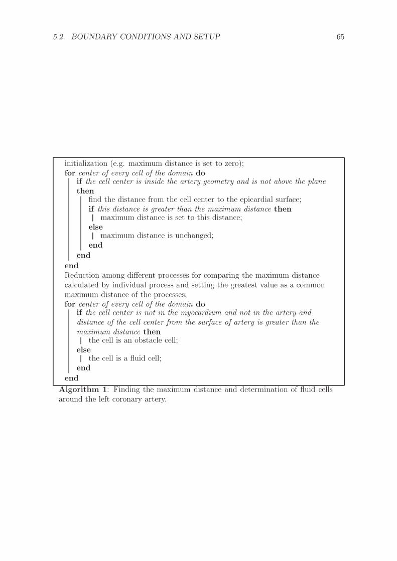
5.2. BOUNDARY CONDITIONS AND SETUP 65

initialization (e.g. maximum distance is set to zero);for center of every cell of the domain do

if the cell center is inside the artery geometry and is not above the planethen

find the distance from the cell center to the epicardial surface;if this distance is greater than the maximum distance then

maximum distance is set to this distance;else

maximum distance is unchanged;end

end

endReduction among different processes for comparing the maximum distancecalculated by individual process and setting the greatest value as a commonmaximum distance of the processes;for center of every cell of the domain do

if the cell center is not in the myocardium and not in the artery anddistance of the cell center from the surface of artery is greater than themaximum distance then

the cell is an obstacle cell;else

the cell is a fluid cell;end

end

Algorithm 1: Finding the maximum distance and determination of fluid cellsaround the left coronary artery.


(a) Valve plane, below which the portion of the geometry is con-sidered the left ventricle.

(b) Anterior view of the structured meshwith extended porous region.

(c) Posterior view of the structured mesh withextended porous region.

Figure 5.5: The setup and structured mesh of GEOM1.


(a) Clipped portion of the mesh with epi-cardium.

(b) Clipped portion of the mesh with endo-cardium.

(c) Boundary conditions for myocardiummesh.

(d) Full view of the structured mesh.

Figure 5.6: Clipped portion of the structured mesh and boundary conditions of GEOM1.


(a) Plane, below which the portion of the geometry is consideredthe left ventricle.

(b) Anterior view of the structured mesh with ex-tended porous region.

(c) Posterior view of the structured meshwith extended porous region.

Figure 5.7: The setup and structured mesh of GEOM2.


(a) Clipped portion of the mesh with epi-cardium.

(b) Clipped portion of the mesh with endo-cardium.

(c) Boundary conditions for myocardiummesh.

(d) Full view of the structured mesh.

Figure 5.8: Clipped portion of the structured mesh and boundary conditions of GEOM2.


5.3 Simulations and Results

The blood is considered as an incompressible Newtonian fluid for simulating the my-ocardial perfusion. The density (ρ) is considered as 1.06g/cm3 and dynamic viscosity(µ) as 0.04dynes/cm2 [78]. The permeability (K) of the myocardium is assumed to be1e−10cm2 [18] and porosity (ǫ) of 0.06. The diastolic mean pressures at the aorta andinside the left ventricle is taken for the boundaries for the simulation purpose (Figure2.3). At inlet for the left coronary artery, 75mmHg pressure has been considered andat the inner wall of the endocardium a pressure of 8mmHg has been considered forthe outlet boundary condition (1mmHg = 1, 333.22368dyne/cm2).

For GEOM1, the lattice constant is considered as, ∆x = 4e−4cm and time interval∆t = 1.81197e − 08sec. For GEOM2, ∆x = 3e − 4cm and ∆t = 1.01923e − 08sec.For both the geometries relaxation time constant, τ = 0.512821 (1/τ ≈ 1.95) is taken.The simulation starts with zero velocity and gradient of pressure. The code runs for75 × 103 time steps for both setups. The lima cluster of Regionales RechenZentrumErlangen (RRZE) is used for the simulations. 36 cores have been used to run the casesfor both setups. The code with the setup of GEOM1 runs for approximately 2 hoursand 30 minutes, whereas; with the setup of GEOM2 runs for approximately 8 hoursand 20 minutes.

The velocity and pressure fields of GEOM1 is shown in Figures 5.9 and 5.10. ForGEOM2, Figures 5.11 and 5.12 depict the velocity and pressure fields, respectively.It can be seen that the higher magnitude velocity region in the myocardium mesh issituated near to the coronary mesh. The pressure is also higher at those regions. Asthe permeability is very small the fluid flow is restricted in other regions. The higherlimits and lower limits of the velocity and pressure fields are fixed to suitable valuesfor effective visualization purposes.

It can be said from the Figures 5.9, 5.10, 5.11 and 5.12 that, the simulation ofperfusion in the myocardium depends on how well the geometries of the coronaryarteries are considered during simulation. Thus, it is also very important that thegeometries for the left coronary arteries are derived well from the CT scan dataset. Asfor the myocardial geometries, as the details are not much complex, it is well capturedmost of the time and simulation of the myocardial perfusion is also satisfactory ifrequired resolution (∆x) is considered.

5.3. SIMULATIONS AND RESULTS 71

Figure 5.9: Velocity field (lattice unit) in pseudocolor after 75 × 103 time steps inGEOM1, full domain (left) and clipped domain (right). ∆x = 4e− 4cm.

Figure 5.10: Pressure field (lattice unit) in pseudocolor after 75 × 103 time steps inGEOM1, full domain (left) and clipped domain (right). ∆x = 4e− 4cm.


Figure 5.11: Velocity field (lattice unit) in pseudocolor after 75 × 103 time steps inGEOM2, full domain (left) and clipped domain (right). ∆x = 3e− 4cm.

Figure 5.12: Pressure field (lattice unit) in pseudocolor after 75 × 103 time steps inGEOM2, full domain (left) and clipped domain (right). ∆x = 3e− 4cm.

73

Chapter 6

Summary

The theoretical chapters review the cardiovascular system, hemodynamics and porousmedium models. It helps to understand the physics of the heart and nature of theblood. The theory of the resistance of different sizes of arteries, arterioles and capil-laries on flow also helps to identify the important vessels which should be consideredduring modeling the myocardial perfusion. Different models of porous medium andtheir application areas are discussed in brief, especially; their limitations and devia-tions from one model to another model is highlighted. The generalized model of porousmedium was selected for the modeling of myocardial perfusion as it offers wide rangeof options, e.g. linearity and non-linearity of the flow with the Brinkman term.

In the chapter about the LBM, the details of the scheme are summarized. Thisis a mesoscopic method and situated between microscopic (discrete) and macroscopicworld (continuum). Though the numerical approach of the method is different fromother continuum based schemes, the NSE can be derived from the LBM. The complexpart of the scheme lies in treating the boundaries of the domain. The boundary condi-tions are implemented by using the discrete distribution functions. The nature of LBMis suitable for simulating the porous medium flows. Different approaches have beenfollowed so far, applying no-slip condition at the pore boundary or adding the dragforces as a force term in the LBE. The GLBMPM considers the linear and non-lineardrag forces of the medium as well as the forces associated with the fluid flow. Thepresence of Brinkman term makes it more flexible by dealing with the interface of thefluid and porous region without explicitly considering the boundary.

This method of myocardial perfusion modeling can be considered as one of the ad-vantages of LBM. The interface between two different media can be dealt with easilyas already discussed before. This is only possible because of the nature (local collisionand streaming) of the scheme unlike other numerical schemes. The computer coderuns for longer time to simulate the results. Geometries of two different patients havebeen considered to examine the flexibility of the method. It has been found that thelattice constant (∆x) should be chosen carefully to satisfy the stability of the scheme.The importance of the details, of the left coronary artery geometries is also understoodfrom the simulation results.

The computer code is tested for the lid driven cavity flow and the couette flow to

74 CHAPTER 6. SUMMARY

examine the outcome. It has been found that the computer code can produce resultsof these fluid dynamics problems with accuracy comparable to the related literature.The method for simulating the myocardial perfusion is also developed considering anarbitrary geometry. This is done to match the human physiology.

75

Chapter 7

Conclusion

The Lattice Boltzmann Method is continuously proving a strong numerical scheme incomparison to other numerical schemes since it’s inauguration. The method gainedmuch attention due to it’s simplicity of implementation on the one hand, and wideoptions for research on the other. Moreover, it’s high scalable feature and ability tosolve large scale problems in parallel environments make it unique in this field. Thelocal nature of the scheme makes it flexible to model new theories for fluid flows indifferent environments and conditions. In this thesis, one of such models is used tosimulate the myocardial perfusion.

A method for simulating the left ventricular myocardial perfusion by LBM hasbeen presented. The tedious coupling between the two geometries and between twodifferent media (continuous fluid and porous media) have been simplified by exploitingthe nature of the Brinkman term in the generalized model for porous medium. Thisterm ensures the continuity of velocity field across the interface of the two differentmedia. The present method considers the drag forces of the porous medium as bodyforces, which also removes the complexity of modeling the porous material packing.The generalized model of porous medium for the porous medium flow considers the lin-earity and non-linearity associated with the flow. It is also found that the myocardialperfusion simulation greatly depends on the left coronary artery geometries. Detailedstructures at the arteriole level could be helpful, which demands further studies. Pa-tient specific modeling needs a dynamic as well as flexible approach and this methodcould provide helpful suggestions for future developments.

The simulation results by the current computer code is also compared with lit-erature data for some well known fluid dynamics problems and showed reasonableaccuracy. The three dimensional lattice cells have been used to predict the two dimen-sional flow. This study showed that the computer code can reproduce the literaturedata associated with the theory.

For further studies with the model, next steps may include:

1. Simulating case studies by not considering the non-linearity of the flow (Fǫ = 0),and comparing it with the total solution of the model. This will help us tounderstand if the expansive computation is actually required and feasible.

2. Implementing non-Newtonian characteristics of the flow and comparing with the

76 CHAPTER 7. CONCLUSION

Newtonian model, if the difference is tolerable.

3. Qualitative and quantitive comparison of the model with the actual phyiologicaldata (myocardial perfusion scan).

In a nutshell, a new application of the generalized model of porous medium hasbeen presented in this thesis. The simulations of myocardial perfusion with patientspecific geometries showed expected results with the simplified current approach. Themethod needs further studies to verify it’s applicability.

77

Chapter 8

References

1. Cardiovascular diseases (CVDs) fact sheets, World Health Organization,UpdatedMarch 2013

2. C. A. Taylor and C. A. Figueroa, Patient-Specific Modeling of CardiovascularMechanics, Annu. Rev. Biomed. Eng. 2009. 11:109–34

3. Frangos S. G., Gahtan V., Sumpio B., Localization of Atherosclerosis: Role ofHemodynamics, Arch Surg. 1999 Oct,134(10):1142-9.

4. M. E. DeBakey, G. M. Lawrie, D. H. Glaeser, Patterns of Atherosclerosis andTheir Surgical Significance, Ann. Surg. 1985; 201:115-131.

5. Jan Götz, Numerical Simulation of Blood flow in Aneurysms using the LatticeBoltzmann Method, Master Thesis, 2006 ,University of Erlangen.

6. Charles A. Taylor, Mary T. Draney, Joy P. Ku, David Parker, Brooke N. Steele,Ken Wang, and Christopher K. Zarins, Predictive Medicine: ComputationalTechniques in Therapeutic Decision-Making, Computer Aided Surgery 4:231–247(1999)

7. N. Westerhof, C. Boer, R. R. Lamberts and P. Sipkema, Cross-Talk BetweenCardiac Muscle and Coronary Vasculature, Physiol Rev 86: 1263–1308, 2006

8. J. M. Huyghe, D. H. V. Campen,T. Arts and R. M. Heethaar, A Two PhaseFinite Element Model of the Diastolic Left Ventricle, J. Bmmechanics Vol. 24,No. 7, pp. 527-538, 1991

9. A. N. Cookson, J. Lee, C. Michler, R. Chabiniok, E. Hyde, D. A. Nordsletten,M. Sinclair, M. Siebes, N. P. Smith, A Novel Porous Mechanical Framework forModelling the Interaction Between Coronary Perfusion and Myocardial Mechan-ics, J. of Biomechanics 45(2012)850–855

10. Qianqian Fang, Sava Sakadžić, Lana Ruvinskaya, Anna Devor, Anders M. Dale,and David A. Boas, Oxygen Advection and Diffusion in a Three Dimensional Vas-cular Anatomical Network,Opt Express. 2008 October 27; 16(22): 17530–17541.

11. F. N. van de Vosse and M. E. H van Dongen, Cardiovascular Fluid Mechanics -Lecture Notes, Eindhoven University of Technology, 1998

78 CHAPTER 8. REFERENCES

12. Richard E. Klabunde, Cardiovascular Physiology Concepts, Second Edition, 2012,ISBN 978-1-4511-1384-6

13. Kris Dumont, Experimental and Numerical Modeling of Heart Valve Dynamics,PhD thesis, 2004, Ghent University.

14. Ali Nasimi, The Cardiovascular System-Physiology, Diagnostics and Clinical Im-plications,2012, Chapter 5, Hemodynamics, InTech, ISBN 978-953-51-0534-3

15. Edward W. Merrill, Rheology of Blood, Physiological Reviews, Vol. 49, No. 4,October 1969

16. Donald A. Nield and Adrian Bejan, Convection in Porous Media, ISBN: 0-387-29096-6,2006 Springer Science+Business Media, Inc.

17. Zhaoli Guo and T. S. Zhao, Lattice Boltzmann Model for Incompressible FlowsThrough Porous Media, Phy. Rev. E 66, 036304 2002

18. Giuliana Elisa Rossi, Numerical Simulation of Perfusion in the Beating Heart,Mater’sThesis 2006 - 2007, Politecnico Di Milano

19. M von Lüdinghausen, Clinical Anatomy of Cardiac Veins, Vv. Cardiacae, SurgRadiol Anat (1987) 9 : 159-168

20. Anthony J. Weinhaus and Kenneth P. Roberts, Chapter 5: Anatomy of theHuman Heart, Paul A. Iaizzo, Handbook of Cardiac Anatomy, Physiology, andDevices, pringer Science Business Media, LLC 2009, ISBN 978-1-60327-371-8

21. Stephen N. Oesterle, Nicolaus Reifart, Eugen Hauptmann, Motoya Hayase, AlanC. Yeung, Percutaneous In Situ Coronary Venous Arterialization: Report of theFirst Human Catheter-Based Coronary Artery Bypass, Circulation. 2001;103:2539-2543

22. Robert M. Berne, Matthew N. Levy, Bruce M. Koeppen, Bruce A. Stanton,Physiology, 2003, Mosby; 5th edition, ISBN-10: 0323022251

23. Sandro De Gruttola, Kevin Boomsma, and Dimos Poulikakos, ComputationalSimulation of a Non-Newtonian Model of the Blood Separation Process, ArtificialOrgans 29(12):949–959, Blackwell Publishing, Inc.

24. Oguz K. Baskurt, Herbert J. Meiselman, Blood Rheology and Hemodynamics.Seminars in Thrombosis and Hemostasis, 29(5):435-450, 2003.

25. Taha Sochi, Non-Newtonian Rheology in Blood Circulation, 2013,arXiv:1306.2067v1 [physics.flu-dyn]

26. Burgstaler EA. Current Instrumentation of Apheresis. In:McLeod BC, Price TH,Drew MJ, eds. Apheresis: Principles and Practice. Bethesda, MD: AmericanAssociation of Blood Banks, 1997;85–112.

79

27. Shu Chien, Shunichi Usami, Harry M. Taylor, John L. Lundberg, Magnus I.Gregersen, Effects of Hematocrit and Plasma Proteins on Human Blood Rheol-ogy at Low Shear Rates, Journal of Applied Physiology January 1, 1966 vol. 21no. 1 81-87

28. Barbara M. Johnston and Peter R. Johnston, Non-Newtonian Blood Flow inHuman Right Coronary Arteries: Steady State Simulations,J. of Biomechanics (BIO/2002/002779 Version 3)

29. Joshua Boyda, James M. Buick , Simon Green, Analysis of the Casson andCarreau-Yasuda non-Newtonian Blood Models in Steady and Oscillatory Flowsusing the Lattice Boltzmann Method, Phys. Fluids 19, 093103 (2007); doi:10.1063/1.2772250

30. Yong Hyun Kim, Pamela J. VandeVord ,and Joon Sang Lee, Multiphase non-Newtonian Effects on Pulsatile Hemodynamics in a Coronary Artery, nt. J.Numer. Meth. Fluids 2008; 58:803-825

31. Malcolm. M. Cross, Rheology of non-Newtonian Fluids: A New Flow Equationfor Pseudoplastic Systems, J. Colloid Science 20, 417-437 (1965).

32. F. J. H. Gijsen, F. N. van de Vosse, and J. D. Janssen, Wall Shear Stress inBackward-Facing Step Flow of a Red Blood celC Suspension, Biorheology 35:4,5(1998) 263–279

33. J. Bernsdorf, D. Wang, Non-Newtonian Blood Flow Simulation in CerebralAneurysms, Computers and Mathematics with Applications 58 (2009) 1024-1029

34. J Boyd, J Buick and S Green, A Second-order Accurate Lattice Boltzmann non-Newtonian Flow Model, J. Phys. A: Math. Gen. 39 (2006) 14241–14247

35. P. K. Mandal, An Unsteady Analysis of non-Newtonian Blood Flow throughTapered Arteries with a Stenosis, International Journal of Non-Linear Mechanics40 (2005) 151 – 164

36. Rafik Ouared and Bastien Chopard, Lattice Boltzmann Simulations of BloodFlow: Non-Newtonian Rheology and Clotting Processes, Journal of StatisticalPhysics, Vol. 121, Nos. 1/2, October 2005

37. M. Lukacova−Medvid′ova,A. Zauskova, Numerical Modelling of Shear-thinningnon-Newtonian Flows in Compliant Vessels, Int. J. Numer. Meth. Fluids 2007;00:1

38. David N. Ku, Blood Flow In Arteries, Annu. Rev. Fluid Mech. 1997. 29:399–434

39. Alian C. Burton, Relation of Structure to Function of the Tissues of the Wall ofBlood Vessels,Physiological Review 34:619, 1954

40. H. Darcy, Les Fontaines Publiques de la Ville de Dijon, Dalmont, Paris (1856)

41. S. P. Neuman, Theoretical Derivation of Darcy’s Law, Acta echanica 25, 153-170(1977) by Springer-Verlag 1977


42. H. C. Brinkman, A calculation of the Viscous Force Exerted by a Flowing Fluidon a Dense Swarm of Particles, Appl. Sci. Res. 1; 27 1947

43. Bear, J. and Bachmat, Y. Introduction to Modeling of Transport Phenomena inPorous Media, Kluwer Academic, Dordrecht.1990

44. Lundgren, T. S. Slow Flow Through Stationary Random Beds and Suspensionsof Spheres. 1972 J. Fluid Mech. 51, 273-299.

45. P. Forchheimer. Wasserbewegung durch Boden. Zeitschrift des Vereines DeutscherIngenieuer, 45 edition, 1901.

46. S. Ergun, A. A. Orning. Fluid Flow through Randomly Packed Columns andFluidized Beds, Industrial and Engineering Chemistry, 41(6)1179-1184, 1949.

47. P. Nithiarasu, K.N. Seetharamu, and T. Sundararajan, Natural Convective HeatTransfer in a Fluid Saturated Variable Porosity Medium, Int. J. Heat MassTransf. 40, 3955 1997

48. Basak, P., Non-Darcy Flow and its Implications to Seepage Problems. J. Irri-gation Drainage Div. ASCE 103. 1977.

49. J. Carlson, A. Jaffe, and A. Wiles, The Millennium Prize Problems. AmericanMathematical Society, 2006

50. U. Frisch, B. Hasslacher, Y. Pomeau, Lattice Gas Automata for the Navier-StokesEquation, Physical Review Latters, Volume 56, No. 14, 1986

51. U. Frisch, D. d’Humieres,B. Hasslacher,P. Lallemand,Y. Pomeau,J-P. Rivet.,Lattice Gas Hydrodynamics in Two and Three Dimensions,Complex System1987;1:649-707.

52. G. R. McNamara and G. Zanetti, Use of the Boltzmann Equation to SimulateLattice-Gas Automata, Physical Review Latters, Volume 61, No. 20, 1988

53. Liboff R. L., Introduction to the Theory of Kinetic Equations. New York: Wiley,1969.

54. Cyrus K. Aidun and Jonathan R. Clausen, Supplementary Material: Lattice-Boltzmann Method for Complex Flows, Supplemental Material: Annu. Rev.Fluid. Mech. 2010. 42:439-472

55. Sauro Succi, The Lattice Boltzmann Equation for Fluid Dynamics and Beyond,Oxford University Press, Oxford, 2001

56. A. A. Mohamad, Lattice Boltzmann Method, ISBN 978-0-85729-454-8, Springer-Verlag London Limited 2011

57. Bhatnagar PL, Gross EP, Krook M. A Model for Collision Processes in Gases.I. Small Amplitude processes in Charged and Neutral One-component Systems.Phys. Rev. 1954. 94:511–25

81

58. Renwei Mei, Wei Shyy, Dazhi Yu and Li-Shi Luo, Lattice Boltzmann Method for3-D Flows With Curved Boundary. J. of Computational Physics 161, 680–699(2000)

59. Chen Peng, The Lattice Boltzmann Method for Fluid Dynamics: Theory andApplications, 2011, Master’s Thesis, École Polytechnique Fédérale de Lausanne(EPFL), Switzerland

60. Xiaoyi He and Li-Shi Luo, Lattice Boltzmann Model for the IncompressibleNavier-Stokes Equation, J. of Statistical Physics, Vol. 88, Nos. 3/4, 1997

61. A. Artoli, Mesoscopic Computational Haemodynamics, Ph.D. Thesis, 2003, Uni-versity of Amsterdam.

62. R.R. Nourgaliev, T.N. Dinh, T.G. Theofanous, D. Joseph, The Lattice Boltz-mann Equation Method: Theoretical Interpretation, Numerics and Implications,Int. J. of Multiphase Flow 29 (2003) 117–169

63. Li-Shi Luo, Wei Liao, Xingwang Chen, Yan Peng and Wei Zhang, Numericsof the Lattice Boltzmann Method: Effects of Collision Models on the LatticeBoltzmann Simulations, Physical Review E 83, 056710 (2011)

64. Irina Ginzburg, Frederik Verhaeghe and Dominique d’Humières, Two-Relaxation-Time Lattice Boltzmann Scheme: About Parametrization, Velocity, Pressure andMixed Boundary Conditions, Commun. Comput. Phys. Feb 2008, Vol. 3, No.2, pp. 427-478

65. J. Bernsdorf , G. Brenner, F. Durst, Numerical Analysis of the Pressure Dropin Porous Media Flow with Lattice Boltzmann (BGK) Automata, ComputerPhysics Communications 129 (2000) 247–255

66. Ali Ghassemi, Ali Pak, Pore Scale Study of Permeability and Tortuosity for Flowthrough Particulate Media using Lattice Boltzmann Method. Int. J. Numer.Anal. Meth. Geomech. (2010)

67. Orla Dardis and John McCloskey, Lattice Boltzmann Ccheme with Real Num-bered Solid Density for the Simulation of Flow in Porous Media, Physical ReviewE Volume 57, Number 4, April 1998

68. Michael A. A. Spaid and Frederick R. Phelan, Jr., Lattice Boltzmann Methodsfor Modeling Microscale Flow in Fibrous Porous Media, Physics of Fluids (1994-present) 9, 2468 (1997)

69. Michael A. A. Spaid and Frederick R. Phelan Jr, Modeling Void FormationDynamics in Fibrous Porous Media with the Lattice Boltzmann Method, Com-posites Part A 29A (1998) 749–755

70. Nicos S. Martys, Improved Approximation of The Brinkman Equation Using aLattice Boltzmann Method, Phys. Fluids, Vol. 13, No. 6, June 2001

71. David M. Freed, Lattice-Boltzmann Method for Macroscopic Porous Media Mod-eling, Int. J. Mod. Phys. C, 09, 1491 (1998)


72. Qinjun Kang, Dongxiao Zhang, Shiyi Chen, Unified Lattice Boltzmann Methodfor Flow in Multiscale Porous Media. Physical Review, E 66, 056307 (2002)

73. D. A. Nield, The Limitations of the Brinkman-Forchheimer Equation in ModelingFlow in a Saturated Porous Medium and at an Interface. 1991, Int. J. Heat FluidFlow, 12, 269-272

74. K. Vafai, S. J. Kim, On the Limitations of the Brinkman-Forchheimer-extendedEquation, Int. J. Heat and Fluid Flow 16: 11-15, 1995

75. Christian Feichtinger, Design and Performance Evaluation of a Software Frame-work for Multi-Physics Simulations on Heterogeneous Supercomputers, PhDthesis, Department of Computer Science 10, System Simulation, UniversitätErlangen-Nürnberg

76. Jan Kretschmer, Christian Godenschwager, Bernhard Preim, and Marc Stam-minger, Interactive Patient-Specific Vascular Modeling with Sweep Surfaces,IEEE Tran. on Vis. and Comp. Graph., Vol. 19, NO. 12, Dec 2013

77. Yefeng Zheng, Adrian Barbu, Bogdan Georgescu, Michael Scheuering, and DorinComaniciu, Four-Chamber Heart Modeling and Automatic Segmentation for 3DCardiac CT Volumes Using Marginal Space Learning and Steerable Features,IEEE Tran. on Med. Imag. 2008

78. H. J. Kim, I. E. Vignon-Clementel,J. S. Coogan, C. A. Figueroa, K. E. Jansen,and C. A. Taylor, Patient-Specific Modeling of Blood Flow and Pressure in Hu-man Coronary Arteries, Ann. of Bio. Engg., Vol. 38, No. 10, Oct 2010, pp.3195–3209

Documents

Lehrstuhl für Informatik 10 (Systemsimulation) · Lehrstuhl für Informatik 10 (Systemsimulation) Numerical Analysis of Myocardial Perfusion in the Left Ventricle by Lattice Boltzmann