Legislators and their Constituencies:Representation in the 106th Congress∗

Joshua D. ClintonDepartment of Political Science

Stanford UniversityStanford, CA 94305

jclinton@stanford.edu

October 31, 2001

∗The author would like to thank John Ferejohn, Simon Jackman, Keith Krehbiel, AdamMeirowitz and Doug Rivers for comments on pieces of this manuscript. The author wouldalso like to thank the National Science Foundation for the Graduate Fellowship that pro-vided invaluable financial assistance. Previous versions were given at the 2001 AmericanPolitical Science Association Annual Meeting, the 2001 Midwest Political Science As-sociation Annual Meeting and the 2001 Summer Meetings of the Society for PoliticalMethodology.

1

Abstract

The extent to which representatives “represent” the preferencesof their district in roll call voting is fundamental to the endeavor ofunderstanding the nature of electoral institutions. Although a greatdeal of work is devoted to this problem, previous work suffers fromboth an inability to measure sub-constituencies of the type identifiedby Fenno (1978) and problems resulting from the usage of ideal pointestimates. Using survey data from a random probability sample of39,000 respondents and a hierarchical Markov Chain Monte Carlo es-timator, this paper addresses both of these limitations. I find thatnot only are legislators’ revealed preferences related to the preferencesof both the geographic and party constituency, but also that thereis some evidence that the ideology of the party constituency is moreimportant to the representative. No evidence suggests that the natureof this relationship varies with respect to the electoral margin, tenure,or staff allocation decisions of the legislator.

1

Arguably one of the most important questions in political science con-cerns whether elected representatives “represent” their constituents. Broadlystated, the research program consists of determining the extent to which thepolicy preferences of constituents are realized in the voting behavior of theirrepresentative. The more limited issue this paper investigates is the relation-ship between constituency ideology and the voting behavior of representativesin the 1st session of the 106th House. Specifically, I answer the substantivequestions of: who (if anyone) does a representative “represents” when cast-ing a roll call vote, and does this vary with respect to characteristics of therepresentative?

Given the primacy of such questions to the enterprise of political science,it is not surprising that a copious body of work concerns itself with these (andrelated) questions. This paper distinguishes itself from prior investigationsby first using new data to provide for a more expansive characterization ofconstituencies than previously possible, and second, presenting a new esti-mator for estimating and recovering the legislator-constituency relationshipthat escapes the statistical problems of previous estimators. A national ran-dom sample of 39,000 respondents permits the preference measurement ofsubgroups within every congressional district.

In summary form, the paper substantively demonstrates:

• That Fenno’s (1978) emphasis on the importance of multiple constituen-cies is important to understanding legislator-constituency relationshipsin the 106th Congress.

• That representatives are responsive to both geographic and party con-stituencies – although evidence suggests that they are more responsiveto the preferences of the party constituency.

• The responsiveness of legislators to their geographic and party con-stituencies is invariant with respect to the electoral margin of the rep-resentative in the 1998 election, the length of time the representativehas served in the House, or the percentage of staff members allocatedto the district.

Methodologically, the paper:

• Presents data that enables scholars to characterize the preferences ofboth geographic and party constituencies.

• Shows that attempts to uncover the legislator-constituency relation-ship by regressing legislator ideal points estimates (e.g., interest groupscores, NOMINATE (Poole and Rosenthal, 1997), Heckman-Snyderscores (Heckman and Snyder,1997)) on covariates of interest producesproblems for inference.

2

• Present a hierarchical Markov Chain Monte Carlo (MCMC) ideal pointestimator which both escapes these problems and permits researchersto examine different specifications of the legislator-constituency rela-tionship.

• Demonstrates that the statistical problems present in existing estima-tors of the legislator-constituency relationship can adversely affect thevalidity of recovered substantive conclusions.

The outline of the paper is as follows. Section 1 briefly recounts thedescription Fenno offers of the legislator-constituency relationship, as thisdescription offers a useful framework for the analysis in subsequent sections.Section 2 reviews the means by which current assessments of the legislator-constituency relationship are made. I argue that there are several reasonsas to why existing methods (and therefore results) are problematic. I alsopresent new data that remedies the previous inability to measure the pref-erences of groups smaller than the district. Section 3 outlines a hierarchicalMCMC estimator of legislative roll call voting that addresses the statisticalshortcomings of existing estimators by simultaneously estimating the idealpoint estimates and the specified relationship between constituency and leg-islator preferences. Section 4 uses this estimator and the data discussed insection 2 to examine several specifications of this relationship to both deter-mine the importance of accounting for the possible influence of constituenciessmaller than the district and to demonstrate the consequences of ignoring thestatistical problems explored in section 2. Section 5 concludes. Appendix Apresents a more rigorous description of the MCMC estimator of Section 3,and Appendix B provides the WinBUGS code used to estimate the models.

1 A Description of the Legislator-Constituency

Relationship

Fenno’s 1978 exploration of the legislator-constituency relationship in themid-1970’s provides a useful point of departure for this paper’s empiricalexamination. Although Fenno makes explicit his reluctance to generalizebeyond the examined Congresses, given that applicability is an empiricalquestion, this paper examines several facets of the description he offers.1

Fenno describes the district as perceived by the representative as beingcomposed of “concentric constituencies.” The largest population of interest

1It is worth noting that there are (at least) two major differences between the periods.First, the average amount of money spent in contemporary campaigns far exceeds theaverage expenditure during the period that Fenno examines. Second, and related to thefirst difference, the national party is much more involved in contemporary races (Jacobson,1997).

3

to the (re-election centered) representative is that of the geographic con-stituency – consisting of all likely voters in the district. The next mostnumerous grouping of constituents is the re-election constituency, which iscomprised of all those voters whose support the representative thinks shewon in the previous election. The re-election constituency’s impression ofthe representative is consequential to the representative because maintainingthe support of those that elected the representative in the last election is(arguably) the surest way to win the next election.

Two smaller constituencies of considerable interest are the primary andpersonal constituencies. Fenno describes the primary constituency when henotes that “we shall think of these people as the ones the congressman be-lieves would provide his last line of electoral defense in a primary contest”(Fenno, 1978:18). The final (and smallest) constituency of interest is that ofthe personal constituency. This group consists of the representative’s closestconfidants and advisors, upon whom the representative relies for advice andsupport.

Although it may seem odd for the (re-election centered) representativeto ever favor the views of a smaller group over those of larger groups, thisapparent anomaly results from the means by which a political campaignis run in a largely disinterested electorate. In other words, the support ofthe primary and personal constituencies are critical because the organizationand publicity provided by these motivated constituents are indispensable tothe running of a successful campaign in the midst of a largely inattentivegeographic constituency.

As Fenno notes and quotes: “The primary constituency, we would guess,draws a special measure of a congressman’s attention:

When I look around to see who I owe my career to, to see thosepeople who were with me in 1970 when I really needed them andwhen most people thought I couldn’t win – these are the peoplethat I owe.

And it should, therefore, draw a special measure of ours” (Fenno, p.19, 1978).A suggestive illustration of the importance of this relationship presents itselfin the 106th Congress.

On July 17, 2000, Michael Forbes (R,NY-1) decided switch parties andjoin the Democratic party. Despite being a 3 term incumbent, and one ofthe most liberal Republicans, Forbes was defeated in the Democratic pri-mary by 71 year-old librarian Regina Seltzer – whose previous office was atown council seat held more than two decades prior. Although Forbes hadthe backing of the Suffolk County Democratic Party and several “strong”Democratic candidates withdrew from the race under pressure from the Na-tional Democratic Party (who were eager to pick up the seat and thought the

4

election of Forbes was a certainty), Forbes was bested in the Democratic pri-mary by Seltzer, who had only $17,200 in cash-on-hand prior to the primary.(Dougherty, 2000)

The interesting aspect of the example is that not only did Forbes alienatehis (former) primary constituency, but the extent of the alienation was suf-ficient so as to cause them to actively campaign for Seltzer, his Democraticprimary opponent. As reported by the Washington Post (Eilperin, 2000):

Fourteen months ago, Jeff LaCourse was a loyal aide to then-GOP Rep. Michael P. Forbes (N.Y.). But then Forbes suddenlyswitched parties, and LaCourse vowed he would do everythingpossible to ensure the congressman did not win reelection in hisLong Island district...Bolstered by an $80,000 contribution fromthe House GOP campaign committee, New York Republicans senteight mailings to the 1st District’s 20,000 registered Democratsover the past 10 days. One included a report card bearing theheader–“100% Great Work!” –which elaborated inside, “Congrat-ulations, Mike Forbes! You received a perfect score from theChristian Coalition.” Another splashed the image of someonegripping an assault weapon with the line, “If you want one ofthese in your home . . . then Congressman Mike Forbes is onyour side.”

Even Forbes acknowledges the role his alienated primary constituencyplayed when he noted that “This was a classic primary election, where whatwe call ‘the true believers’ turned out. My Democratic opponent had noresources and no ground troops to speak of. They [the alienated Republicans]picked the nominee” (Eilperin, 2000).2 Although Forbes ran in the generalelection as a third party candidate, he performed miserably – getting only3% of the vote.

Despite the clear description offered by Fenno, and the suggestive exampleabove, it is difficult to examine the relative extent to which representativesrespond to the constituencies Fenno describes. This is true not only becauseof their size (in the case of primary and personal constituencies), but alsobecause they are defined in terms of the amount of support they providethe representative. In other words, given that they are defined as being con-stituents with influence, trying to determine if they influence representatives’voting behavior is tautological. However, there is another constituency of po-tential interest to the representative that is both easier to characterize andof theoretical interest.

2Of course, the Republicans were also acting strategically, as by enabling Seltzer towin, they arguably assured themselves of victory in the general election – which they won56% to 41%.

5

[INSERT FIGURE 1 ABOUT HERE]

Figure 1 summarizes the relationship between the party constituency –which consists of every constituent in the district with the same partisanaffiliation as the incumbent – and the constituencies discussed by Fenno. AsFigure 1 shows, the party constituency contains most, if not all, of the pri-mary and personal constituencies. Although outside of Fenno’s discussion,examining the possible relationship between the (revealed) preferences of alegislator and those of her party constituency is of interest not only becausethis determination examines Fenno’s basic point that a legislator is respon-sive to more than just the geographic (or re-election) constituency, but alsobecause the investigation provides evidence as to whether political partiesare important in an electoral context.

There are four reasons as to why the preferences of the party constituencymay be important to the legislator. First, because the party constituencylargely represents the set of constituents who provide the representative withthe organization and resources with which to run re-election campaigns, rep-resentation of the party constituency’s policy preferences may be necessaryin order to obtain this support. Second, given that representatives often pos-sess very little information about the policy preferences of their district, thepartisan affiliation of the party constituency may provide the representativewith an informational cue that they can utilize in determining how to vote ona given roll call. Third, given that the party constituency represents the setof possible (closed) primary voters, representation of the party constituencymay result from the fact that the representative faces both a primary andgeneral election (Aldrich, 1995). Finally, given that the representative can bethought of as being drawn from the set of party constituents in the district,it may be that the preferences of the party constituency actually representthe representatives personal preferences (as would be true in expectation).

Given that any of the four reasons provided above represent sufficient(but not necessary) conditions as to why representatives would vote in ac-cordance with the preferences of the party constituency, it is an empiricalquestion as to the extent to which this occurs. However, the representativemust be responsive to the preferences of the larger constituency, as winningthe support of the party constituency will be of little use if so doing putsthe legislator at odds with the beliefs of the larger constituency. Even so,it is unclear whether the legislator is more responsive to the preferences ofthe geographic or party constituency when casting roll call votes – althoughprevious research into the relationship of the Senate suggests the latter (e.g.,Fort et. al. (1993), Brady and Schwartz (1995), and Levitt (1996))). Be-fore moving to an investigation of the form that the legislator-constituencyrelationship takes in the contemporary Congress, I first argue why existingattempts at this characterization are problematic.

An important caveat to the analysis that follows is that although it is

6

common to think of representation as a conscious decision by the repre-sentative to vote in accordance with the preference of the constituency (assuggested by Mayhew (1974)), an observationally equivalent possibility arisesif the representative ignores the constituency’s preference and votes her ownpreference so long as both have similar preferences.3 Given this causal inde-terminacy, the empirical results cannot determine whether a representativeconsciously votes in accordance with the preferences of her constituency orif she only acts as if she does.

2 Problems with (and Solutions to) the Prob-

lem of Interest

A copious amount of research on the issue of relating legislator and con-stituency preferences exists. Although by no means an exhaustive accountof the attempt, previous research has used: survey data from both the con-stituency and legislator on several issues (e.g., Miller and Stokes (1963),Achen (1977), Achen (1978), Erickson (1978)), on all issues (e.g., Ansolabehereet. al. (2001)), constituency opinion and an estimate of legislator ideology(e.g., Powell (1982), Page et al. (1984)), constituency characteristics andlegislator roll call voting with respect to a specific issue (e.g., Jackson andKing (1989), Bartels (1991), Bailey and Brady (1998), Bailey (2001)), con-stituency characteristics and a roll call derived measure of legislator ideology(e.g., Kau and Rubin (1979), Kau and Rubin (1982)) and constituency pref-erence revealed through initiative voting and estimates of legislator ideology(e.g., Snyder (1996), Gerber and Lewis (2000)). The variety of methodsemployed is evidence of the difficulty associated with the problem.

Two statistical problems have hindered previous attempts at specifyingthe nature of the legislator-constituency relationship. The first, and mostproblematic, concerns Fenno (1978)’s observation/supposition that a districtcontains several constituencies of interest to the legislator. If true, failing toaccount for this possibility results in the statistical problems associated withomitted variable bias.

The second problem is highlighted by realizing that an answer to the ques-tion “who do legislators represent” involves recovering the relationship be-tween three unobservable preferences – those of the legislator, the geographicconstituency, and the party constituency. Although measures are arguablypresent for the latter two quantities, scholars are forced to use estimates of(revealed) preferences for legislators. This creates problems for statistical in-ference because the (heteroskedastic and autocorrelated) error variance of any

3In fact, there are good theoretical reasons to suspect that there are selection effectswhich favor the election of representatives whose ideology is highly correlated to that ofthe constituencies of importance (Zaller, 1998).

7

ideal point estimate is correlated with measures of constituency preference –resulting in incorrect standard error estimates when the typical approach toestimating the relationship is adopted.

2.1 Measuring Constituency Preference

That estimators of the legislator-constituency relationship should account forthe possibility that representatives differentially respond to the preferencesof the various constituencies is not a new observation (e.g., Goff and Grier(1993), Krehbiel (1993)). However, scholars have been limited in their abilityto measure these preferences by a lack of available data.4

The most common measures of constituency preference are the percent-age of two-party votes cast by the district for the Democratic (for example)presidential candidate, and the demographic composition of the district. Al-though using each requires making some (arguably strong) assumptions, themost significant limitation with either measure is that each provides for therecovery of only one “ideal point” per district.5 Such measures consequentlyprovide no ability to determine the extent to which the representatives’ rollcall behavior is consistent with their geographic and/or party constituencies.Absent such an ability, it is impossible to examine the possibility raised byFenno of multiple constituencies within a district.

The inability to measure the party constituency’s preferences results ina very well-known and severe statistical problem. Specifically, if the prefer-ences of the party constituency is correlated with legislators’ roll call votingbehavior, the estimated specification suffers from omitted variable bias – re-sulting in the biased estimation of all parameters of interest (Greene, 1997).Consequently, despite a large literature on the legislator-constituency rela-tionship, it is unclear how much we know given that most previous estimatorssuffer from this problem.

A means of characterizing the preferences of constituencies smaller thanthe geographic constituency is potentially provided by survey data – as ascholar using survey data can exploit relationships between survey responsesto construct measures of interest. Despite this promise, such an approach haspreviously been impossible because of the problems created by insufficientsample sizes, non-random sampling or both.

4The notable attempts that have been made typically focus on the Senate (e.g., Peltz-man (1984), Ladha (1991), Fort et. al. (1993), Brady and Schwartz (1995) Levitt (1996))rather than on the House (e.g., Powell (1982)).

5Using district presidential vote percentage assumes both that presidential voting isideologically driven and either the same ideological issues are present in both the pres-idential and congressional elections, or that the mapping between the ideological issuesfor the two races is consistent. Using demographic measures necessarily introduces spec-ification error, as the researcher is forced to summarize district ideology using availabledemographic characteristics.

8

Most survey based measures rely on data from the National ElectionStudy (e.g., Miller and Stokes (1963), Page et. al. (1984)). Consequently,observations typically exist for only a quarter of the congressional districtsand the average district is characterized by less than 20 observations. Moretroubling is the fact that because some of the samples used are not randomprobability samples because of either sampling issues (e.g., Miller and Stokes(1963)) or selection effects (e.g., Ansolabehere et. al. (2001)), producingvalid estimates requires significant assumptions (and adjustments) for validinference (Smith, 1983).

This paper addresses these shortcomings in survey based measures by us-ing previously unavailable data. Although the preferences of the geographicconstituency are characterized using the average Democratic two-party dis-trict presidential vote in the 1992 and 1996 elections and the preferences ofthe party constituency are constructed using the survey responses of 39,000randomly selected respondents.6 Specifically, the average response to a stan-dard ideological self-placement question for only those respondents in thedistrict whose partisan affiliation is the same as the incumbent characterizesthe party constituencies’ ideology.7 In other words, the measure of a Repub-lican congressman’s party constituency’s is given by the average ideologicalself-placement for only those respondents in the district who identify withthe Republican party. The question used is:

There has been a lot of talk these days about liberals and con-servatives. Would you say that you are...

Very LiberalLiberalModerateConservativeVery ConservativeDon’t know

The 39,000 respondents are distributed such that every congressional dis-trict contains at least 8 respondents. Since the average district contains 88respondents – with the 1st district of Arkansas and the 3rd district of Iowa

6It might be argued that the geographic constituency should also be characterized by asurvey measure. Given the error associated with this measure in citizens with low politicalengagement, there is reason to be wary of the validity of such a measure (Converse (1962,1964)). In addition, it is not clear how informative such a measure would be given that theparty constituency measure is comprised of a subset of these voters (and therefore highlyco-linear) . Specifications using this measure confirm these concerns, as a survey basedmeasure of the geographic constituency’s ideology never obtains statistical significance.

7Note that further subsets such as only those partisans who indicate that they areregistered to vote or only those partisans who describe their partisanship as “strong”produce the same qualitative conclusions.

9

characterized by the fewest number of respondents (8 and 9 respectively) andthe 7th district of Florida and the 4th district of California containing themost respondents (209 and 211 respectively) – it is possible to measure thepreferences of the party constituency in every congressional district.

[INSERT FIGURE 2 ABOUT HERE]

The upper and lower histograms in Figure 2 summarize the number ofrespondents in the geographic and party constituencies respectively. Forpurposes of comparison, the mean number of respondents Miller and Stokes(1963) and Powell (1982) use to summarize the preference of the geographicconstituency (for only 116 and 108 of the districts respectively) is also de-noted. As is immediately evident from Figure 2, this paper uses more datato characterize the preferences of party constituencies than previous survey-based studies use to measure the preference of geographic constituencies.

Before describing the relationship between the preference measures of thegeographic and party constituencies, it is important to describe the dataused. The survey data is from Knowledge Networks, which utilizes randomprobability sampling of the sampling frame consisting of all US householdswith a working telephone line. After sampling, those numbers for whichit is possible to identify an address through reverse address matching aresent a letter informing them that they have been selected to participate inthe Knowledge Networks Panel. In addition to describing the purposes ofthe Panel and the desired respondent commitment level, a small monetaryincentive is provided to encourage cooperation.

All numbers sent a letter, and a fraction of those not sent a letter are thencalled to be recruited to join the Panel. During the call, which typically lasts10-15 minutes, the head of the household is told that in return for memberscompleting a short survey every week, the household will be provided witha free WebTV interactive television unit and free Internet access for theWebTV unit. If recruited, the entire household is enumerated. At the timethat the surveys described in this paper were performed, the cooperation rate(i.e., total number of completes divided by the total number of completesand refusals) was around 56%. Although one might be concerned about thepossibility of panel effects, not only does current research on the KnowledgeNetworks panel suggest that the bias is not large for the period examined(Clinton, 2000), but given that I rely on responses given in the second surveyassigned to panelists, it is doubtful whether sufficient exposure has elapsedto induce such behavior.

Figure 3 depicts the relationship between the (assumed) ideal points of thegeographic and party constituencies. Recall that the survey based measuredescribed above is used to measure the preference of the party constituenciesand the two-party Democratic presidential vote percentage is used to measurethe preference of the geographic constituencies.

10

[INSERT FIGURE 3 ABOUT HERE]

Although correlated at .66, clear differences are immediately evident uponinspection. The vertical line segments in Figure 3 indicate the sample sizeused to summarize the ideology of the party constituency. The height of thesegments is given by the reciprocal of the sample size used. Since the samplesize varies from 2 to 88, the segments’ length accordingly vary from .01 to.5.8

Having described both the first statistical problem confronting scholarsinterested in the nature of the legislator-constituency relationship and thesolution I employ, I now turn to the second.

2.2 Ideal Point Estimates As A Dependent Variable

Since estimates of representatives’ revealed preferences are readily availableto scholars thanks to interest groups and the work of political scientists suchas Poole and Rosenthal (1997), Groseclose et. al. (1999), and Heckman andSnyder (1997), a typical approach to recovering the legislator-constituencyrelationship consists of a variation of the following two-step process (e.g., Kauand Rubin (1979), McCarty et. al. (1997), Brady et. al. (2000), Rothenbergand Sanders (2000), Stratmann (2000)):9

1. Estimate (or find pre-existing estimates of) legislator i’s true ideal pointxi – denoted x̂i, where xi = x̂i + ωi.

2. Regress the ideal point estimates x̂ on the covariates of interest Z usingthe relationship x̂ = Zγ + ε2 and make inferences about the resultingcoefficient estimates γ̂.

As legislator ideal point estimates are estimates, measurement error nec-essarily results. Before demonstrating how statistical inferences are affectedby the measurement error ω of the (step 1) ideal point estimates, I first

8It is well known that sampling error is introduced into the measure because the partyconstituency’s preference is based on aggregated survey results (Achen (1977), Achen(1978), ?, Powell (1982), Jackson (1989)). The hierarchical estimator described in section3 permits scholars to account for this variation by also incorporating a measurement errormodel for the preference of the party constituency. This work is currently underway andpreliminary evidence suggests that the paper’s substantive conclusions are robust to thissampling error.

9Although not discussed, it is clear that the “residual regression” approach of Kauand Rubin (1979) and Carson and Oppenheimer (1984) is subject to the same criticismoutlined below. Specifically, and independent of the criticisms of Poole (1988) and Benderand Lott (1996), because of measurement error in the ideal point estimates, the error fromthe “purging” regression will reflect this measurement error. As this measurement errordiffers across legislators, one cannot simply interpret the regression error as “shirking”.

11

establish the characteristics of this measurement error. Specifically, the mea-surement error is: 1) heteroskedastic, 2) (spatially) autocorrelated, and 3) itsvariance is correlated with covariates of interest to the legislator-constituencyrelationship.10

As the top left graph of figure 4 makes clear, using the MCMC estimatorof Clinton et. al. (2001) on the first session of the 106th House reveals thatthe ideal point estimates of extremist legislators are measured with moreuncertainty than centrist legislators.11

[INSERT FIGURE 4 ABOUT HERE]

This pattern occurs because of the (relative) lack of proposals with extremecut-points – resulting in diminished ability to discriminate among extremelegislators (e.g., it does not often happen that Maxine Waters (D,CA-35)finds a bill too liberal for her liking). In other words, the variance of themeasurement error is not constant across legislators because of the nature ofthe data generating process.

Given that the variance in the ideal point estimates is related to the ideo-logical extremity of the legislator, it is clear that the variance of the estimatesis related to any covariate that attempts to measure the ideological prefer-ence of the district. The top right graph of figure 4 confirms this intuition.It depicts the relationship between the standard errors of the MCMC idealpoint estimates and the average two party percent Democratic presidentialvote in the district. As the line summarizing the loess regression of the mea-surement error variance on the district’s Democratic presidential vote makesexplicit, there is a (non-linear) relationship between the two quantities.

Finally, the fact that the measurement error is also (spatially) autocor-related can be realized by observing that the spatial nature of the problemimplies that ideologically similar legislators will possess similar amounts ofuncertainty. This occurs because the spatial voting model underlying theideal point estimator expects ideologically similar legislators to vote simi-larly. Thus, the same mistakes will be made for ideologically similar legisla-tors conditional on the recovered cutpoint. In other words, since the locationof the cutpoints is recovered with error, this will necessarily introduce er-ror into the ideal point estimates – with ideologically proximate legislatorsbeing similarly affected. The bottom two graphs of Figure 4 confirm thatthis covariation exists. Uncorrelated measurement errors would result in asymmetric joint MCMC ideal point posterior distribution – as the fact thatlegislator i is more liberal than average on iteration t implies nothing aboutthe location of legislator j on iteration t. This is precisely what we find in

10Note that the claim does not depend on the estimates being systematically biased.11A similar relationship results when using W-NOMINATE estimates and their (condi-

tional) bootstrapped standard errors.

12

the lower right graph, which graphs the relationship between the most lib-eral member in the 1st session of the 106th Congress (Waters (D,CA-35))and most conservative member (Stump (R,AZ-3)). This contrasts greatly tothe pattern recovered in the lower left graph – which graphs Waters againstthe second most liberal in the session (Filner (D,CA-50)). These two graphsillustrate that the errors of the ideal point estimates covary depending onspatial proximity.

The intuition as to why the two-step procedure produces standard errorsthat are too small is provided by Figure 5.

[INSERT FIGURE 5 ABOUT HERE]

The top two graphs in Figure 5 depict the extent of measurement errorin Y conditional on X when the truth is Y=X. In the top-left graph, themeasurement error of Y is larger for extreme values of X. As Figure 4 makesclear, this is the case scholars face when using the two-step approach. Thetop-right graph depicts a case where the measurement error is invariant withrespect to X.

The lower graphs depict the area in which the best linear predictor willbe found given the measurement error in Y. The observation of interest isthat the “band” in which the best linear predictor will be found is “taller”in the lower-left graph than the lower-right graph. This indicates that theuncertainty associated with the measure of Y introduces relatively more un-certainty into the recovered relationship between X and Y.

The (textbook) result can also be proven analytically. Assuming that theideal point measurement error ω and the second stage regression errors ε2

are uncorrelated (i.e., E(ωε′2) = E(ε2ω′) = 0), it is straightforward to show:

V ar(γ) = E[(γ̂ − γ)(γ̂ − γ)′]= E[((Z ′Z)−1Z ′(Zγ + ω + ε2)− γ)((Z ′Z)−1Z ′(Zγ − ω + ε2)− γ)′]= E[(Z ′Z)−1Z ′(ε2ε

′2 − ε2ω

′ − ωε′2 − ωω′)Z(Z ′Z)−1

= (Z ′Z)−1Z ′σ2ε2

IZ(Z ′Z)−1 + (Z ′Z)−1Z ′WZ(Z ′Z)−1

= σ2ε2

(Z ′Z)−1 + (Z ′Z)−1Z ′WZ(Z ′Z)−1

6= σ2ε2

(Z ′Z)−1

where W = E(ωω′) represents the variance-covariance matrix of ideal pointmeasurement errors. Thus, the standard errors of a regression which ignoresthe measurement error are too small by a factor of (Z ′Z)−1Z ′WZ(Z ′Z)−1

so long as E(Z ′W ) 6= 0 (i.e., the variance of the measurement error is corre-lated with the covariates of interest). An alternative characterization of theproblem is to realize that the errors in the second stage errors are both het-eroskedastic and autocorrelated, with the variance-covariance matrix givenby: (Z ′Z)−1Z ′(σ2

ε2I + W )Z(Z ′Z)−1.

13

3 An Empirical Model of Roll Call Voting

It is (unfortunately) impossible to address this problem using widely-used es-timators of legislator ideal points. Interest group scores and factor analyticmeasures such as Heckman-Snyder (1997) provide no uncertainty assessmentsby definition (although it is theoretically possible to derive the latter (Ander-son and Amemiya, 1988). Although NOMINATE and its derivatives can the-oretically provide such measures because of their maximum-likelihood foun-dation, the recovery of the uncertainty assessments has proven to be practi-cally impossible because of the computational inability to invert extremelylarge matrices. Consequently, the reported standard errors of NOMINATEare created by bootstrapping over the conditional likelihood (and cannot re-cover the covariance terms in W ).12 As Poole and Rosenthal themselveswarn: “the standard errors produced by the D-NOMINATE algorithm mustbe viewed as heuristic descriptive statistics” (Poole and Rosenthal 1997: 246).

Given these problems, to account for the uncertainty in ideal point esti-mates I utilize a hierarchical MCMC estimator. As the posterior distributionof a Bayesian estimator is defined over all model parameters, uncertaintyin the ideal point estimates will correctly propogate throughout the model(Draper, 1995). Thus, the coefficients of the regression of legislator idealpoint estimates on constituency characteristics will account for the uncer-tainty of the ideal point estimates. The remainder of this section brieflydescribes the hierarchical MCMC estimator used to estimate the legislator-constituency relationship. Appendix A contains a more technical (and com-plete) derivation.

The parameterization of the problem of recovering ideal points from amatrix of “ones and zeros” using a Bayesian framework is well documented(e.g., Clinton et. al. (2001), Jackman (2000), Jackman (2001), Clinton andMeirowitz (2001)) – as is its formulation in item response models in theeducational testing literature (e.g., Johnson and Albert (1999)). To incor-porate covariates into the framework, instead of assuming that every idealpoint has a common prior distribution (e.g., xi ∼ N(0, 1)), the hierarchicalmodel allows the mean of the prior distribution to vary by legislator (e.g.,xi ∼ N(µxi, τ

2)). In other words, the model is hierarchical because priorparameters µx and τ 2 (typically called “hyperparameters”) are estimated.

The prior mean for the legislators’ ideal points µx is assumed to be givenas a linear function of the covariates of interest. In other words, the functionalform of the relationship is given by: µx = Zγ + ε2, where Z represents theL×k matrix of constituency/legislator covariates and γ denotes the k-lengthcoefficient vector associated with the least squares solution of regressing µx

12Poole and Rosenthal bootstrap ideal point estimates assuming bill parameters areperfectly measured, and they (separately) bootstrap the bill parameter estimates assumingthe ideal points are perfectly measured.

14

on Z.13 The estimation of τ 2 permits the variance of the ideal point priorto depend upon the fit of the hierarchical structure for µx. Estimating ahierarchical structure permits the simultaneous recovery of both legislatorideal points and the relationship between the covariates of interest and thelegislator ideal points by maximizing the joint likelihood function of the idealpoint problem (step one) and the linear regression problem (step two).

That the hierarchical MCMC estimator accounts for the hetereoskedasticand autocorrelated measurement error present in the legislator ideal pointestimates can be seen by considering the fact that at each iteration the idealpoint estimates of the previous iteration are regressed on the covariates ofinterest. Thus, as the ideal point estimates fluctuate between iterations (re-flecting the uncertainty associated with their estimation), so too will thecoefficient values for the regression.

4 Estimation of the Legislator-Constituency

Relationship

This section uses the estimator developed in section 3 and the preferencemeasures described in section 2 to estimate the legislator-constituency rela-tionship of the 106th House during the 1st session.14 As a complete inves-tigation of which district preferences the legislator is responsive to and whyis beyond the scope of this paper, the investigations of this section aim to:determine whether the preferences of the party constituency are influential(because of any one of the four reasons advanced in section 1), demonstratethe consequences of ignoring the statistical problems described in section 2,and begin to characterize the extent to which legislators’ (revealed) prefer-ences are responsive to constituency preferences.

To examine the possibility that legislators in the 1st session of the 106thHouse are responsive to both their party and geographic constituencies, Ioperationalize the relationship using the following specification of µXi:

15

µxi = γ1Geographic Constituency Ideology (mean-deviated)+γ2Party Constituency Ideology(mean-deviated) + ε2i

(1)

with ε2i ∼ N(0, τ 2). This specification assumes that a legislator’s prefer-ence can be decomposed into a portion due to each constituency. Note that

13Due to the iterative nature in which these tasks are performed, this statement is notquite precise enough. Appendix A clarifies this point.

14Estimating the examined specifications using the 2nd session produce substantivelyidentical results.

15Note that the covariates are mean deviated to improve the mixing of the Gibbs Sampler(Gilks and Roberts, 1996).

15

because the constituency preferences are measured using different scales, es-timating a separate personal preference for the legislators is unidentified (incontrast to the approach of Levitt (1996)).

The specification of equation 1 is estimated four ways to provide fora robust comparison: using ordinary least squares (OLS) with the non-hierarchical MCMC ideal point estimates of Clinton et. al. (2001), using(non-hierarchical) Bayesian linear regression, using generalized least squares(GLS) and weighting by the standard error of the ideal point measurementerror (Greene, 1997), and using the hierarchical MCMC estimator of sec-tion 3. As Table 1 shows, because the priors of the estimators are identicalwhere applicable, the only difference between the estimators is the hierarchi-cal structure.16 Consequently, any resulting differences not due to samplingerror can be attributed to the absence of this structure.

Table 1: Priors for the hierarchical and non-hierarchical estimatorsHierarchical Two-Step Two-Step

Parameter Estimator Estimator (Bayes) Estimator (OLS/GLS)γ ∼ N(0, 42) ∼ N(0, 42) NAτ 2 ∼ Γ(.05, .05) NA NAX ∼ N(Zγ, τ 2) ∼ N(0, 12) ∼ N(0, 42)α ∼ N(0, 42) ∼ N(0, 42) ∼ N(0, 42)β ∼ N(0, 42) ∼ N(0, 42) ∼ N(0, 42)

Although multiple chains and thinning is employed so as to maximize theparameter space examined by the estimator, parameter estimates of the 453non-lopsided roll calls and 435 legislators stabilize quickly.17 For purposesof interpretation, recall that negative ideal point estimates represent liberalvoting behavior.

Interpreting the results is less than straight-forward because several ob-servationally equivalent interpretations are possible (using any estimator).First, it could be that the representative consciously votes according to thepreferences of the geographic and party constituencies (i.e., direct represen-tation occurs). It is also possible that the legislator votes her own ideal point– which happens to covary with the preferences of the constituencies (e.g.,indirect representation occurs).18 Third, it could be that the representativevotes according to the preferences of a third agent (e.g., interest groups), but

16The priors for X,α and β for the two-step estimators are the priors from the idealpoint estimation of the first step.

17Although assessing stochastic convergence is more of an art than a science (roughlyequivalent to determining whether one has obtained a local or global minimum in amaximum-likelihood framework), nothing suggests that the reported estimates have notconverged.

18Of course, given that representatives face continually re-election, there is every reasonto suspect that selection effects produce this covariation.

16

that the resulting votes happen to produce an “ideology” that covaries withthe preferences of the constituencies. Finally, it could be the case that thepreferences of the party constituencies are irrelevant and the districts’ me-dian voter is actually an (identical) combination of the measures employed(and not the measure I use as the geographic constituencies’ preferences).Thus, despite the ability to recover the covariation between the legislatorsrevealed ideal point and the (assumed) preferences of the geographic andparty constituencies, this model is unable to address the long standing ques-tion of whether the findings represent evidence of direct, indirect or accidentalrepresentation.

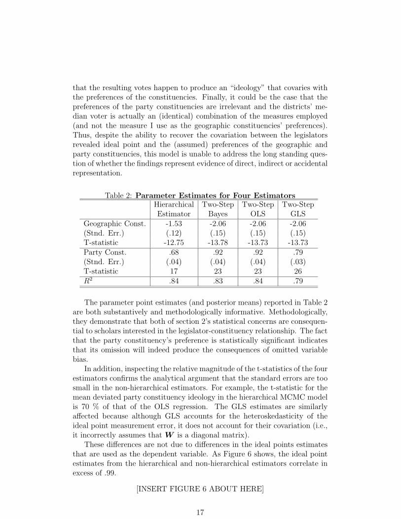
Table 2: Parameter Estimates for Four EstimatorsHierarchical Two-Step Two-Step Two-StepEstimator Bayes OLS GLS

Geographic Const. -1.53 -2.06 -2.06 -2.06(Stnd. Err.) (.12) (.15) (.15) (.15)T-statistic -12.75 -13.78 -13.73 -13.73Party Const. .68 .92 .92 .79(Stnd. Err.) (.04) (.04) (.04) (.03)T-statistic 17 23 23 26R2 .84 .83 .84 .79

The parameter point estimates (and posterior means) reported in Table 2are both substantively and methodologically informative. Methodologically,they demonstrate that both of section 2’s statistical concerns are consequen-tial to scholars interested in the legislator-constituency relationship. The factthat the party constituency’s preference is statistically significant indicatesthat its omission will indeed produce the consequences of omitted variablebias.

In addition, inspecting the relative magnitude of the t-statistics of the fourestimators confirms the analytical argument that the standard errors are toosmall in the non-hierarchical estimators. For example, the t-statistic for themean deviated party constituency ideology in the hierarchical MCMC modelis 70 % of that of the OLS regression. The GLS estimates are similarlyaffected because although GLS accounts for the heteroskedasticity of theideal point measurement error, it does not account for their covariation (i.e.,it incorrectly assumes that W is a diagonal matrix).

These differences are not due to differences in the ideal points estimatesthat are used as the dependent variable. As Figure 6 shows, the ideal pointestimates from the hierarchical and non-hierarchical estimators correlate inexcess of .99.

[INSERT FIGURE 6 ABOUT HERE]

17

Note that scale differences in the ideal point estimates (which accounts forthe differences in the coefficient point estimates) result because whereas theMCMC ideal point estimator “shrinks” legislators towards the common priormean (of 0), the hierachical model “shrinks” legislator ideal points towardstheir predicted ideal points (which is recovered using the covariate informa-tion).19

Substantively, legislators’ revealed ideal points covary with the prefer-ences of both the geographic and party constituencies. Thus, although thereare no necessary reasons as to why legislators ought to vote in a manner re-lated to the preferences of the party constituency, such responsiveness exists.For example, districts with a higher support for Clinton than average (i.e., apositive geographic constituency measurement) or with party constituenciesmore liberal than average (i.e., a positive party constituency measurement)both predict a more liberal (i.e., negative) revealed ideal point. The speci-fication is an extremely good fit, as the OLS specification is able to explain84 % of the observed variation in the ideal point estimates.

Although the finding that the revealed legislator ideal point covaries withthe preference of both the geographic and party constituencies is an impor-tant and novel finding, it is also of interest as to which constituency is “moreimportant” to the representative. As noted by Powell (1982) and Levitt(1996), determining which constituency is more important is very difficultgiven that the preferences of the geographic and party constituencies aremeasured using different scales. A measures of the relative influence of eachconstituency is possible despite this difficulty.

Specifically, I consider the extent to which a constituency’s preferencesmust change to offset a one-standard deviation shift in the preferences of theother constituency. In other words, if the (mean-deviated) Clinton two-partyvote increases by 1 standard deviation in the district (i.e., Clinton’s vote per-centage increases by 12.5 %), the preference of the party constituency has tobecome more conservative by .28 (on a 5 point integer scale) to offset thischange. This is equivalent to around half of a standard deviation change inparty constituency ideology. Conversely, if the party constituency becomes 1standard deviation more liberal (i.e., the average ideology falls by .49) Clin-ton’s two party vote percentage has to increase by 22% (around 2 standarddeviations) to offset the change. The fact that a two standard deviationchange in the preferences of the geographic constituency is required to offseta one standard deviation change in the preference of the party constituencyprovides evidence that the legislator is more responsive to the preferences ofthe party constituency.

19The result is also not due to an overly informative prior distribution for γ. Tighteningthe prior variance from 17 to 1 recovers a posterior mean (standard deviation) of -1.51(.12) for the geographic constituency and .68 (.04) for the party constituency.

18

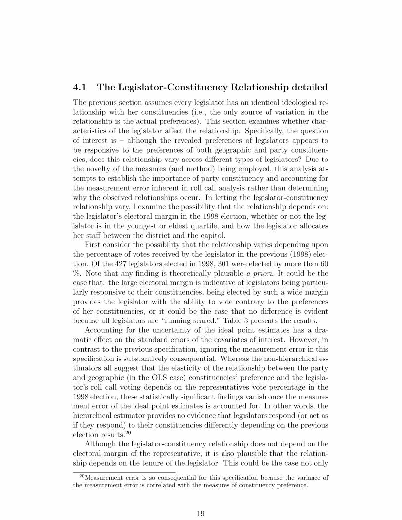
4.1 The Legislator-Constituency Relationship detailed

The previous section assumes every legislator has an identical ideological re-lationship with her constituencies (i.e., the only source of variation in therelationship is the actual preferences). This section examines whether char-acteristics of the legislator affect the relationship. Specifically, the questionof interest is – although the revealed preferences of legislators appears tobe responsive to the preferences of both geographic and party constituen-cies, does this relationship vary across different types of legislators? Due tothe novelty of the measures (and method) being employed, this analysis at-tempts to establish the importance of party constituency and accounting forthe measurement error inherent in roll call analysis rather than determiningwhy the observed relationships occur. In letting the legislator-constituencyrelationship vary, I examine the possibility that the relationship depends on:the legislator’s electoral margin in the 1998 election, whether or not the leg-islator is in the youngest or eldest quartile, and how the legislator allocatesher staff between the district and the capitol.

First consider the possibility that the relationship varies depending uponthe percentage of votes received by the legislator in the previous (1998) elec-tion. Of the 427 legislators elected in 1998, 301 were elected by more than 60%. Note that any finding is theoretically plausible a priori. It could be thecase that: the large electoral margin is indicative of legislators being particu-larly responsive to their constituencies, being elected by such a wide marginprovides the legislator with the ability to vote contrary to the preferencesof her constituencies, or it could be the case that no difference is evidentbecause all legislators are “running scared.” Table 3 presents the results.

Accounting for the uncertainty of the ideal point estimates has a dra-matic effect on the standard errors of the covariates of interest. However, incontrast to the previous specification, ignoring the measurement error in thisspecification is substantively consequential. Whereas the non-hierarchical es-timators all suggest that the elasticity of the relationship between the partyand geographic (in the OLS case) constituencies’ preference and the legisla-tor’s roll call voting depends on the representatives vote percentage in the1998 election, these statistically significant findings vanish once the measure-ment error of the ideal point estimates is accounted for. In other words, thehierarchical estimator provides no evidence that legislators respond (or act asif they respond) to their constituencies differently depending on the previouselection results.20

Although the legislator-constituency relationship does not depend on theelectoral margin of the representative, it is also plausible that the relation-ship depends on the tenure of the legislator. This could be the case not only

20Measurement error is so consequential for this specification because the variance ofthe measurement error is correlated with the measures of constituency preference.

19

Table 3: Responsiveness by Electoral Margin

Hierarchical Two-Step Two-Step Two-StepEstimator Bayes OLS GLS

Geographic Const. -1.34 -2.61 -2.61 -2.27(Stnd. Err.) (.29) (.18) (.18) (.17)T-statistic -4.62 -16.17 -16.17 -13.35Party Const. .41 .88 .88 .78

(.06) (.04) (.04) (.03)T-statistic 6.83 22 22 2698 Margin .0007 .0016 .0016 .0009

(.001) (.0009) (.001) (.0009)T-statistic .7 1.77 1.6 198 Margin × .02 .02 .02 .009Geographic Const. (.02) (.01) (.01) (.01)T-statistic 1 2 2 .998 Margin × .0004 -.007 -.007 -.006Party Const. (.0004) (.002) (.002) (.002)T-statistic 1 -3.5 -3.5 -3R2 .33 .84 .85 .80

because senior legislators may be more aware of the preferences of their dis-trict (and therefore respond to the preferences in a different manner), butalso because seniority may provide legislators with an ability to vote contraryto district preferences (for example). To investigate this possibility, legisla-tors are classified based upon the number of years served in the House andI examine if the relationship of the upper quartile differs from that of thelower quarter (or those in neither quartile).21 The lower quartile contains the119 members who have served less than 4 years in the House and the upperquartile consists of the 114 members who have served more than 14 years inthe House. Table 4 presents the results.

As is immediately evident from Table 4, none of the estimators suggestthat the legislator-constituency relationship depends upon the tenure of thelegislator.

Finally, I consider whether the responsiveness of the legislator depends onthe percentage of staff (in the Summer of 2000) the legislator allocates to thedistrict (Congressional Quarterly Staff Directory, 2000). This is of interestto determine if the relationship of a service-based representative (i.e., major-ity of staff allocated to district office(s)) differs from that of a policy-basedrepresentative (i.e., majority of staff allocated to Washington D.C. office).Empirically, it is of interest because it permits the determination whether

21Restricting the examination to freshman representatives reveals no systematic differ-ence in the relationship between freshman and non-freshman representatives.

20

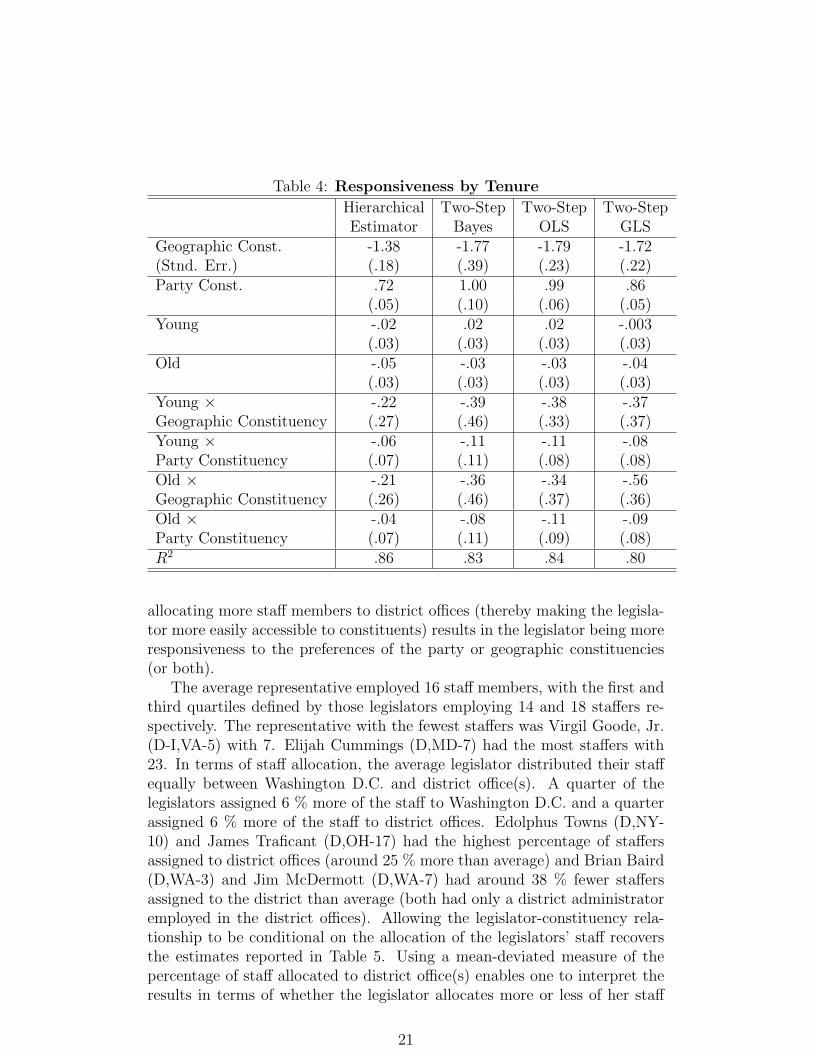
Table 4: Responsiveness by Tenure

Hierarchical Two-Step Two-Step Two-StepEstimator Bayes OLS GLS

Geographic Const. -1.38 -1.77 -1.79 -1.72(Stnd. Err.) (.18) (.39) (.23) (.22)Party Const. .72 1.00 .99 .86

(.05) (.10) (.06) (.05)Young -.02 .02 .02 -.003

(.03) (.03) (.03) (.03)Old -.05 -.03 -.03 -.04

(.03) (.03) (.03) (.03)Young × -.22 -.39 -.38 -.37Geographic Constituency (.27) (.46) (.33) (.37)Young × -.06 -.11 -.11 -.08Party Constituency (.07) (.11) (.08) (.08)Old × -.21 -.36 -.34 -.56Geographic Constituency (.26) (.46) (.37) (.36)Old × -.04 -.08 -.11 -.09Party Constituency (.07) (.11) (.09) (.08)R2 .86 .83 .84 .80

allocating more staff members to district offices (thereby making the legisla-tor more easily accessible to constituents) results in the legislator being moreresponsiveness to the preferences of the party or geographic constituencies(or both).

The average representative employed 16 staff members, with the first andthird quartiles defined by those legislators employing 14 and 18 staffers re-spectively. The representative with the fewest staffers was Virgil Goode, Jr.(D-I,VA-5) with 7. Elijah Cummings (D,MD-7) had the most staffers with23. In terms of staff allocation, the average legislator distributed their staffequally between Washington D.C. and district office(s). A quarter of thelegislators assigned 6 % more of the staff to Washington D.C. and a quarterassigned 6 % more of the staff to district offices. Edolphus Towns (D,NY-10) and James Traficant (D,OH-17) had the highest percentage of staffersassigned to district offices (around 25 % more than average) and Brian Baird(D,WA-3) and Jim McDermott (D,WA-7) had around 38 % fewer staffersassigned to the district than average (both had only a district administratoremployed in the district offices). Allowing the legislator-constituency rela-tionship to be conditional on the allocation of the legislators’ staff recoversthe estimates reported in Table 5. Using a mean-deviated measure of thepercentage of staff allocated to district office(s) enables one to interpret theresults in terms of whether the legislator allocates more or less of her staff

21

to the district than average.22

Table 5: Relationship by Staff Allocation

Hierarchical Two-Step Two-Step Two-StepEstimator Bayes OLS GLS

Geographic Constituency -1.54 -2.11 -2.11 -2.12(Stnd. Err.) (.12) (.16) (.15) (.15)Party Constituency .67 .91 .92 .78

(.04) (.04) (.04) (.03)Staff Allocation -.04 -.06 -.06 -.06

(.11) (.16) (.15) (.14)Staff Allocation × 1.79 2.73 2.94 4.01Geographic Constituency (1.03) (1.358) (1.45) (1.47)Staff Allocation × .55 .70 .74 .83Party Constituency (.30) (.39) (.41) (.35)R2 .84 .83 .84 .79

As in previous specifications, ignoring the measurement error of the idealpoint estimates and using OLS leads one to (incorrectly) conclude that therelationship between the legislator and her geographic constituency dependson the relative percentage of staff allocated to the district.23 The resultsof the hierarchical estimator indicates that the roll call behavior of legis-lators identically covaries with the preferences of the geographic and partyconstituencies irrespective of how legislators allocate their staff.

The fact that all legislators respond to (or act as if they respond to)the preferences of both constituencies while giving priority to the prefer-ences of the party constituency indicates that Fenno is exactly right to stressthe importance of constituencies smaller than the geographic constituency.That the legislator-constituency relationship for the 1st session of the 106thCongress is invariant with respect to the three examined legislator charac-teristics suggests that (at least in terms of the characteristics examined) theobserved relationship represents an optimal response to the (identical) se-lection pressures facing representatives (i.e., repeated primary and generalelections). That being said, it is important to recall that it is impossible todetermine whether legislators consciously cultivate this relationship or if se-lection effects created by repeated primary and general elections self-selectsthose legislators who unconsciously form this ideological relationship.

Furthermore, the recovery of identical ideological legislator-constituencyrelationships does not imply either that representatives’ “home styles” are in-

22The results are also robust to using the number of district offices or the number ofdistrict staffers.

23Using GLS would lead one to believe that the relationship with both the party andgeographic constituency are affected.

22

consequential or that all representatives employ an identical home style. Theresults instead suggest that legislators are able to maintain identical ideolog-ical relationships despite differences in the manner in which they interactwith their constituencies (e.g., the percentage of staff that they allocate tothe district). In other words, there are multiple ways for a representative torespond to the ideological preferences of her district.

One might also wonder how a representative ever loses given the resultthat all legislators adopt the identical and (inferred to be) optimal ideologi-cal relationship with their constituencies. Two explanations of this apparentcontradiction suggest themselves. First, reasons/circumstances apart fromthe general ideological relationship of the legislator and her constituents maysometimes be decisive. For example, a scandal may deleteriously affect theelectoral fortune of a representative even if the representative maintains theoptimal relationship. Second, despite maintaining the optimal relationshipon average, a legislator’s “incorrect” votes on a handful of highly salientissues may prove to be more important to constituents than the general ide-ological agreement of the legislator and her constituents (the fate of MarjoleMargolies-Mezvinsky (D,PA-13) in the 1994 election is often used as the pro-totypical example) (e.g., Brady et. al. 2000)).

5 Conclusion

The task of recovering the legislator-constituency relationship is both funda-mental to political science and extremely difficult. Answering the questioninvolves uncovering the relationship between unobservable quantities usingcrude measures. Consequently, making inferences about the general natureof the legislator-constituency relationship is exceedingly difficult.

Previous attempts at quantifying the legislator-constituency relationshiphave been limited by statistical problems resulting from both an inabilityto measure the preferences of constituencies smaller than the geographicconstituency and the consequences of using ideal point estimates as the de-pendent variable of interest. Both of these concerns are addressed using newdata and a new estimator.

Substantively, I am able to utilize the survey responses of 39,000 respon-dents to determine whether Fenno’s observations that i] within any district,several constituencies exist, and ii] some constituencies (i.e., the party con-stituency) appear more important to the representative than others are ap-plicable to the contemporary Congress. Using a hierarchical MCMC idealpoint estimator, I determine that in the 1st session of the 106th Congress,Fenno is right on both accounts. There is also no evidence that the ideologi-cal basis of the legislator-constituency relationship varies with respect to theelectoral margin of the representative in the previous election, the tenure ofthe representative, or the percentage of staff the representative allocates to

23

district offices(s) relative to Washington D.C..These substantive insights are possible because of the two methodological

contributions made by the paper. Specifically, I demonstrate that inferencebased on estimators which fail to address these two concerns will produceboth biased estimates (as a consequence of omitting the preferences of theparty constituency) and standard errors which are too small (as a conse-quence of the ideal point measurement errors). Consequently, it is unclearhow valid the inferences from prior examinations are given that most fail toaccount for these concerns.

Despite these insights, understanding the relationship between constituencypreferences and the roll call behavior of the legislators requires not only acharacterization of what the relationship is, but also why it is. Although thispaper only sketches the latter, it provides scholars with a foundation withwhich to conduct the former. Specifically, the findings paper suggest thatthe relationship is more nuanced than simply voting the preferences of thedistrict’s “median voter.” Instead, and in terms of the analysis conductedthus far, the representative appears to balance the demands of the party andgeographic constituencies. The (obvious) next step is to use the advancesin this paper to conduct a characterization of the relationship in concertwith derived theoretical implications so as to permit an understanding ofwhy it is that the observed relationship between constituency and legislatorpreferences obtains.

24

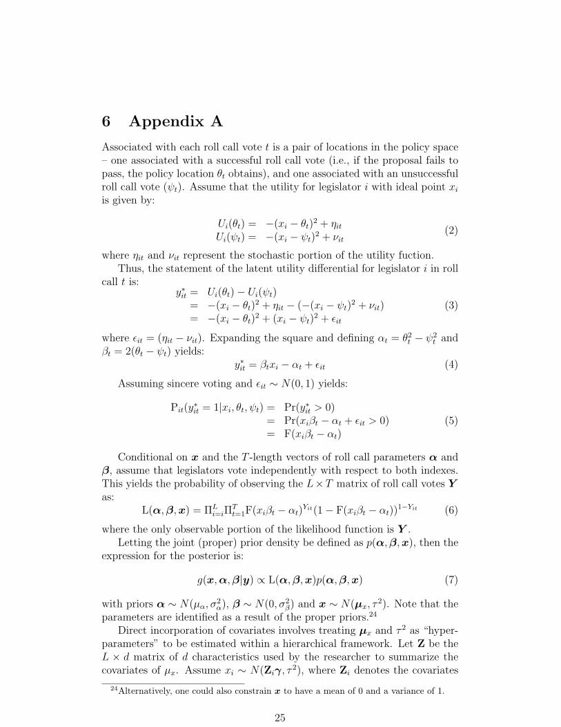
6 Appendix A

Associated with each roll call vote t is a pair of locations in the policy space– one associated with a successful roll call vote (i.e., if the proposal fails topass, the policy location θt obtains), and one associated with an unsuccessfulroll call vote (ψt). Assume that the utility for legislator i with ideal point xi

is given by:

Ui(θt) = −(xi − θt)2 + ηit

Ui(ψt) = −(xi − ψt)2 + νit

(2)

where ηit and νit represent the stochastic portion of the utility fuction.Thus, the statement of the latent utility differential for legislator i in roll

call t is:y∗it = Ui(θt)− Ui(ψt)

= −(xi − θt)2 + ηit − (−(xi − ψt)

2 + νit)= −(xi − θt)

2 + (xi − ψt)2 + εit

(3)

where εit = (ηit − νit). Expanding the square and defining αt = θ2t − ψ2

t andβt = 2(θt − ψt) yields:

y∗it = βtxi − αt + εit (4)

Assuming sincere voting and εit ∼ N(0, 1) yields:

Pit(y∗it = 1|xi, θt, ψt) = Pr(y∗it > 0)

= Pr(xiβt − αt + εit > 0)= F(xiβt − αt)

(5)

Conditional on x and the T -length vectors of roll call parameters α andβ, assume that legislators vote independently with respect to both indexes.This yields the probability of observing the L×T matrix of roll call votes Yas:

L(α,β,x) = ΠLi=iΠ

Tt=1F(xiβt − αt)

Yit(1− F(xiβt − αt))1−Yit (6)

where the only observable portion of the likelihood function is Y .Letting the joint (proper) prior density be defined as p(α,β,x), then the

expression for the posterior is:

g(x,α,β|y) ∝ L(α,β,x)p(α,β,x) (7)

with priors α ∼ N(µα, σ2α), β ∼ N(0, σ2

β) and x ∼ N(µx, τ2). Note that the

parameters are identified as a result of the proper priors.24

Direct incorporation of covariates involves treating µx and τ 2 as “hyper-parameters” to be estimated within a hierarchical framework. Let Z be theL × d matrix of d characteristics used by the researcher to summarize thecovariates of µx. Assume xi ∼ N(Ziγ, τ

2), where Zi denotes the covariates

24Alternatively, one could also constrain x to have a mean of 0 and a variance of 1.

25

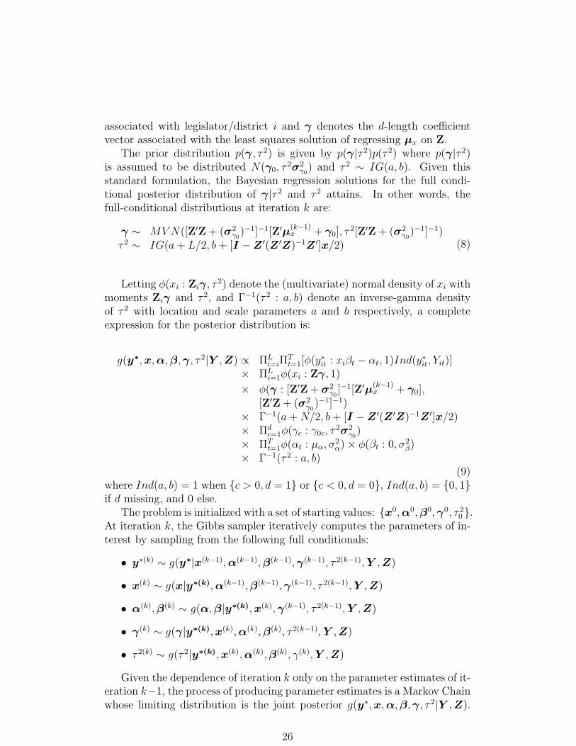
associated with legislator/district i and γ denotes the d-length coefficientvector associated with the least squares solution of regressing µx on Z.

The prior distribution p(γ, τ 2) is given by p(γ|τ 2)p(τ 2) where p(γ|τ 2)is assumed to be distributed N(γ0, τ

2σ2γ0

) and τ 2 ∼ IG(a, b). Given thisstandard formulation, the Bayesian regression solutions for the full condi-tional posterior distribution of γ|τ 2 and τ 2 attains. In other words, thefull-conditional distributions at iteration k are:

γ ∼ MVN([Z′Z + (σ2γ0

)−1]−1[Z′µ(k−1)x + γ0], τ

2[Z′Z + (σ2γ0

)−1]−1)τ 2 ∼ IG(a+ L/2, b+ [I −Z ′(Z ′Z)−1Z ′]x/2) (8)

Letting φ(xi : Ziγ, τ2) denote the (multivariate) normal density of xi with

moments Ziγ and τ 2, and Γ−1(τ 2 : a, b) denote an inverse-gamma densityof τ 2 with location and scale parameters a and b respectively, a completeexpression for the posterior distribution is:

g(y∗,x,α,β,γ, τ 2|Y ,Z) ∝ ΠLi=iΠ

Tt=1[φ(y∗it : xiβt − αt, 1)Ind(y∗it, Yit)]

× ΠLi=1φ(xi : Zγ, 1)

× φ(γ : [Z′Z + σ2γ0

]−1[Z′µ(k−1)x + γ0],

[Z′Z + (σ2γ0

)−1]−1)× Γ−1(a+N/2, b+ [I −Z ′(Z ′Z)−1Z ′]x/2)× Πd

c=1φ(γc : γ0c, τ2σ2

γ0)

× ΠTt=1φ(αt : µα, σ

2α)× φ(βt : 0, σ2

β)× Γ−1(τ 2 : a, b)

(9)where Ind(a, b) = 1 when {c > 0, d = 1} or {c < 0, d = 0}, Ind(a, b) = {0, 1}if d missing, and 0 else.

The problem is initialized with a set of starting values: {x0,α0,β0,γ0, τ 20 }.

At iteration k, the Gibbs sampler iteratively computes the parameters of in-terest by sampling from the following full conditionals:

• y∗(k) ∼ g(y∗|x(k−1),α(k−1),β(k−1),γ(k−1), τ 2(k−1),Y ,Z)

• x(k) ∼ g(x|y∗(k),α(k−1),β(k−1),γ(k−1), τ 2(k−1),Y ,Z)

• α(k),β(k) ∼ g(α,β|y∗(k),x(k),γ(k−1), τ 2(k−1),Y ,Z)

• γ(k) ∼ g(γ|y∗(k),x(k),α(k),β(k), τ 2(k−1),Y ,Z)

• τ 2(k) ∼ g(τ 2|y∗(k),x(k),α(k),β(k), γ(k),Y ,Z)

Given the dependence of iteration k only on the parameter estimates of it-eration k−1, the process of producing parameter estimates is a Markov Chainwhose limiting distribution is the joint posterior g(y∗,x,α,β,γ, τ 2|Y ,Z).

26

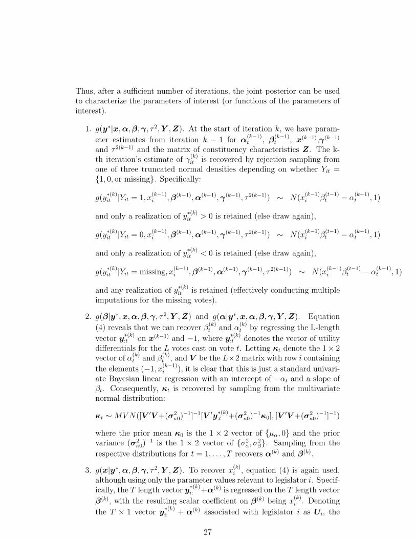
Thus, after a sufficient number of iterations, the joint posterior can be usedto characterize the parameters of interest (or functions of the parameters ofinterest).

1. g(y∗|x,α,β,γ, τ 2,Y ,Z). At the start of iteration k, we have param-

eter estimates from iteration k − 1 for α(k−1)t , β

(k−1)t , x(k−1),γ(k−1)

and τ 2(k−1) and the matrix of constituency characteristics Z. The k-th iteration’s estimate of γ

(k)it is recovered by rejection sampling from

one of three truncated normal densities depending on whether Yit ={1, 0, or missing}. Specifically:

g(y∗(k)it |Yit = 1, x

(k−1)i ,β(k−1),α(k−1),γ(k−1), τ 2(k−1)) ∼ N(x

(k−1)i β

(t−1)t − α

(k−1)t , 1)

and only a realization of y∗(k)it > 0 is retained (else draw again),

g(y∗(k)it |Yit = 0, x

(k−1)i ,β(k−1),α(k−1),γ(k−1), τ 2(k−1)) ∼ N(x

(k−1)i β

(t−1)t − α

(k−1)t , 1)

and only a realization of y∗(k)it < 0 is retained (else draw again),

g(y∗(k)it |Yit = missing, x

(k−1)i ,β(k−1),α(k−1),γ(k−1), τ 2(k−1)) ∼ N(x

(k−1)i β

(t−1)t − α

(k−1)t , 1)

and any realization of y∗(k)it is retained (effectively conducting multiple

imputations for the missing votes).

2. g(β|y∗,x,α,β,γ, τ 2,Y ,Z) and g(α|y∗,x,α,β,γ,Y ,Z). Equation

(4) reveals that we can recover β(k)t and α

(k)t by regressing the L-length

vector y∗(k):t on x(k−1) and −1, where y

∗(k):t denotes the vector of utility

differentials for the L votes cast on vote t. Letting κt denote the 1× 2vector of α

(k)t and β

(k)t , and V be the L×2 matrix with row i containing

the elements (−1, x(k−1)i ), it is clear that this is just a standard univari-

ate Bayesian linear regression with an intercept of −αt and a slope ofβt. Consequently, κt is recovered by sampling from the multivariatenormal distribution:

κt ∼MVN([V ′V +(σ2κ0)

−1]−1[V ′y∗(k):t +(σ2

κ0)−1κ0], [V

′V +(σ2κ0)

−1]−1)

where the prior mean κ0 is the 1 × 2 vector of {µα, 0} and the priorvariance (σ2

κ0)−1 is the 1 × 2 vector of {σ2

α, σ2β}. Sampling from the

respective distributions for t = 1, . . . , T recovers α(k) and β(k).

3. g(x|y∗,α,β,γ, τ 2,Y ,Z). To recover x(k)i , equation (4) is again used,

although using only the parameter values relevant to legislator i. Specif-ically, the T length vector y

∗(k)i: +α(k) is regressed on the T length vector

β(k), with the resulting scalar coefficient on β(k) being x(k)i . Denoting

the T × 1 vector y∗(k)i: + α(k) associated with legislator i as Ui, the

27

standard Bayesian regression results obtain. Hence, with a N(Zγ, 1)

prior, x(k)i is sampled from:

xi ∼ N([β(k)′β(k) + I]−1[β(k)′Ui + Zγ(k−1)], [β(k)′β(k) + I−1]−1)

This regression is performed L times (once for each i ∈ L) to generatethe vector x(k).

4. g(γ|y∗,x,α,β, τ 2,Y ,Z) and g(τ 2|y∗,x,α,β,γ,Y ,Z). Assuming alinear functional form, γ(k) and τ 2(k) are recovered via a Bayesian linearregression of x(k) on Z. As discussed above, the conditional posteriordistributions of γ(k) and τ 2(k) are given in equation (8).

28

7 Appendix B

######################################

## Josh Clinton

## Stanford University

## WinBUGS Code for Specification 1

######################################

# Variables in Model

# N (indexed by i) = number of Legislators

# M (indexed by j) = number of roll call votes

# g.id = geographic constituency ideology (Avg. \% Clinton Vote in district)

# p.id = party constituency ideology (survey measure)

{ for (i in 1:N){

for (j in 1:M){

mu[i,j] <- beta[j,1]*x[i] - beta[j,2]; # Mean utility differential

# for legislator i on roll call j

h106ystar[i,j] ~ dnorm(mu[i,j],1.0)I(h106lower[i,j],h106upper[i,j]);

# Truncated Normal Sampling

# for latent utility

}

}

for (i in 1:N){ # Structural Component

of Ideal Point

mux[i] <- coef[1]*g.id[i] + coef[2]*p.id[i] # Expression for prior mean

x[i] ~ dnorm(mux[i],sigma) # Ideal point prior distribution

}

# Define Prior Distributions

for(j in 1:M){

beta[j,1:2] ~ dmnorm(0.0, B[1:2,1:2]) # Item discrimination [1]

} # and difficulty [2] priors

coef ~ dmnorm(b[1:2],B[1:2,1:2])

sigma ~ gamma(a,b)

tau2 <- 1/sigma # BUGS uses precisions

}

29

References

Achen, Cristopher H. 1977. “Measuring Representation: Perils of the Corre-lation Coefficient.” American Journal of Poltical Science 21:805–15.

Achen, Cristopher H. 1978. “Measuring Representation.” American Journalof Poltical Science 22:475–510.

Aldrich, John H. 1995. Why Parties? The Origin and Transformation ofPolitical Parties in America. Chicago: University of Chicago Press.

Anderson, T.W. and Yasuo Amemiya. 1988. “The Asymptotic Normal Distri-bution of Estimators in Factor Analysis under General Conditions.” Annalsof Statistics 16:759–771.

Ansolabehere, Stephen, James M. Snyder J. and III Charles Stewart. 2001.“Candidate Positioning in U.S. House Elections.” American Journal ofPolitical Science 45:136–59.

Bailey, Michael. 2001. “Quiet Influence: The Representation of DiffueseInterests on Trade Policy, 1983-94.” Legislative Studies Quarterly 26:45–80.

Bailey, Michael and David W. Brady. 1998. “Heterogeneity and Representa-tion: The Senate and Free Trade.” American Journal of Political Science42:524–44.

Bartels, Larry M. 1991. “Constituency Opinion and Congressional PolicyMaking: The Reagan Defense Buildup.” American Poltical Science Review85:457–473.

Bender, Bruce and Jr. John R. Lott. 1996. “Legislator Voting and Shirking:A Critical Review of the literature.” Public Choice 87:67–100.

Brady, David, Brandice Canes-Wrone and John Cogan. 2000. Continuityand Change in House Elections. “Differences in Legislative Voting Behav-ior Between Winning and Losing House Incumbents” Stanford: StanfordUniversity Press pp. 178–192. ed. David Brady, John Cogan and MorrisFiorina.

Brady, David and Edward P. Schwartz. 1995. “Ideology and Interests inCongressional Voting: The Politics of Abortion in the U.S. Senate.” PublicChoice 84:25–48.

Carson, Richard T. and Joe A. Oppenheimer. 1984. “A Method of Estimat-ing the Personal Ideology of Political Representation.” American PolticalScience Review 78:163–78.

30

Clinton, Joshua D. 2000. “Panel Bias from Attrition and Conditioning: ACase Study of the Knowledge Networks Panel.” Stanford University type-script.

Clinton, Joshua D. and Adam Meirowitz. 2001. “Agenda Constrained Legis-lator Ideal Points and the Spatial Voting Model.” Political Analysis 9:242–259.

Clinton, Joshua D., Simon Jackman and Doug Rivers. N.d. “The StatisticalAnalysis of Roll Call Data.” Presented at 2000 Meetings of the Society forPolitical Methodology.

Congressional Staff Directory. 2000. Washington D.C.: Congressional Quar-terly. ed. Joel D. Treese.

Converse, Philip E. 1962. “Information Flow and the Stability of PartisanAttitudes.” Public Opinion Quarterly 26:578–599.

Converse, Philip E. 1964. Ideology and Discontent. “The Nature of BeliefSystems in Mass Publics” New York: Free Press. ed. David E. Apter.

Dougherty, Suzanne. 2000. “N.Y. Rep. Forbes Likely Upset in Pri-mary.” Congressional Quarterly. URL: http://washingtonpost.com/wp-dyn/politics/elections/2000/states/ny/house/ny01/A60386-2000Sep13.html.

Draper, David. 1995. “Assessment and Propogation of Model Uncertainty.”Journal of the Royal Statistical Society, Series B (Methodological) 57:45–97.

Eilperin, Juliet. 2000. “With Stealth, GOP Turns Tables on Turncoat Rep.Forbes.” Washington Post.

Erickson, Robert S. 1978. “Constituency Opinion and Congressional Behav-ior: A Reexamination of the Miller-Stokes Representation Data.” Ameri-can Poltical Science Review 22:511–35.

Fenno, Richard F. 1978. Home Style: House Members in Their Districts.Boston: Little, Brown and Company.

Gerber, Elisabeth R. and Jeffrey B. Lewis. 2000. “Representing Heteroge-neous Districts.” Working paper.

Gilks, W. R. and G. O. Roberts. 1996. Markov Chain Monte Carlo in Prac-tice. “Strategies for Improving MCMC” New York: Chapman & Hallpp. 115–127. ed. W.R. Gilks, S. Richardson, and D.J. Spiegelhalter.

31

Goff, B.L. and K.B. Grier. 1993. “On the (mis)Measurment of LegislatorIdeology and Shirking.” Public Choice 76:5–20.

Greene, William H. 1997. Econometric Analysis. 3rd ed. New Jersey:Prentice-Hall.

Groseclose, Tim, Steven D. Levitt and Jr. James M. Snyder. 1999. “Com-paring Interest Group Scores Across Time and Chambers: Adjusted ADAScores for the U.S. Congress.” American Political Science Review 93:33–50.

Heckman, James J. and Jr. James M. Snyder. 1997. “Linear ProbabilityModels of the Demand for Attributes with an Empirical Application toEstimating the Preferences of Legislators.” Rand Journal of Economics28:S142–S169.

Jackman, Simon. 2000. “Estimation and Inference Are Missing Data Prob-lems: Unifying Social Science Statistics via Bayesian Simulation.” PolticalAnalysis 8:307–22.

Jackman, Simon. 2001. “Multidimensional Analysis of Roll Call Data viaBayesian Simulation: Identifiation, Estimation, Inference, and ModelChecking.” Political Analysis 9:227–241.

Jackson, John E. 1989. “An Errors-in-Variables Approach to EstimatingModels in Small Area Data.” Political Analysis 1:157–80.

Jackson, John E. and David C. King. 1989. “Public Goods, Private Interests,and Representation.” American Poltical Science Review 83:1143–64.

Jacobson, Gary C. 1997. The Politics of Congressional Elections. 4 ed. NewYork: Longman.

Johnson, Valen E. and James H. Albert. 1999. Ordinal Data Modeling. NewYork: Springer.

Kau, James B. and Paul H. Rubin. 1979. “Self-Interest, Ideology and Lo-golling in Congressional Voting.” Journal of Law and Economics 22:365–384.

Kau, James B. and Paul H. Rubin. 1982. Congressmen, Constituents andContributors: Determinants of Roll Call Voting in the House of Represen-tatives. Studies in Public Choice Boston: Martinus Nijhoff Publishing.

Krehbiel, Keith. 1993. “Constituency characteristics and legislative prefer-ences.” Public Choice 76:21–37.

Ladha, Krishna K. 1991. “A Spatial Model of Legislative Voting with Per-ceptual Error.” Public Choice 68:151–74.

32

Levitt, Stephen. 1996. “How Do Senators Vote? Disentangling the Roleof Voter Preferences, Party Affiliation, and Senator Ideology.” AmericanEconomic Review 86:425–41.

Mayhew, David R. 1974. Congress: The Electoral Connection. New Haven:Yale University Press.

McCarty, Nolan, Keith T. Poole and Howard Rosenthal. 1997. Income Re-distribution and the Realignment of American Politics. AEI Studies onUnderstanding Economic Inequality Washington DC: American EnterpriseInstitute.

Miller, Warren E. and Donald E. Stokes. 1963. “Constituency Influence inCongress.” American Political Science Review 57:45–56.

Page, Benjamin I., Robert Y. Shapiro Paul W. Gronke Robert M. Rosen-berg. 1984. “Constituency, Party and Representation in Congress.” PublicOpinion Quarterly 48:741–56.

Peltzman, Sam. 1984. “Constituent Interest and Congressional Voting.”Journal of Law and Economics 27:181–210.

Poole, Keith. 1988. “Recent Developments In Analytical Models of VotingIn the U.S. Congress.” Legislative Studies Quarterly 13:117–133.

Poole, Keith T. and Howard Rosenthal. 1997. Congress: A Political-Economic History of Roll Call Voting. New York: Oxford University Press.

Powell, Lynda W. 1982. “Issue Representation in Congress.” The Journal ofPolitics 44:658–78.

Rodney Fort, William Hallagan, Cyril Morong and Tesa Stegner. 1993. “TheIdeological Component of Senate Voting: Different Principles or DifferentPrincipals.” Public Choice 76:39–57.

Rothenberg, Lawrence S. and Mitchell S. Sanders. 2000. “Severing the Elec-toral Connection: Shirking in the Contemporary Congress.” AmericanJournal of Poltical Science 44:316–325.

Smith, T.M.F. 1983. “On the Validity of Inferences from Non-Random Sam-ple.” Journal of the Royal Statistical Society. Series A 146:394–403.

Snyder, James M. 1996. “Constituency Preferences: California Ballot Propo-sitions: 1974-90.” Legislative Studies Quarterly 21:463–488.

Stratmann, Thomas. 2000. “Congressional Voting over Legislative Careers:Shifting Positions and Changing Constraints.” American Political ScienceReview 94:665–676.

33

Zaller, John. 1998. Party Politics and Politicians. “Politicians as Prize Fight-ers: Electoral Selection and Incumbency Advantage” Baltimore: JohnHopkins University Press. ed. John Geer.

34

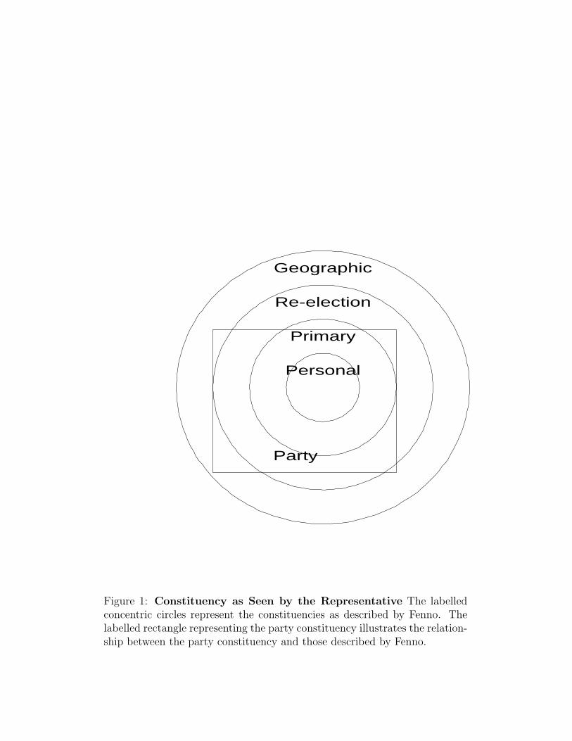
Personal

Primary

Re-election

Geographic

Party

Figure 1: Constituency as Seen by the Representative The labelledconcentric circles represent the constituencies as described by Fenno. Thelabelled rectangle representing the party constituency illustrates the relation-ship between the party constituency and those described by Fenno.

0 50 100 150 200

020

4060

8010

0

Number of Respondents In Geographic Constituency

Num

ber o

f Dis

trict

s

Mean (88)

Miller & Stokes

Powell

0 50 100 150 200

050

100

150

200

Number of Respondents In Party Constituency

Num

ber o

f Dis

trict

s

Mean (36)

Miller & Stokes

Powell

Figure 2: Sample Sizes of the Constituencies The upper (lower) histro-gram presents the number of respondents in the geographic (party) con-stituency. For purposes of comparison, the labeled lines denote the meansample sizes used by several previous studies.

oo

o

o

o

o

o

o

o

o

o

o

o

o

o

o

o

o

o

oo

o

o

o

oo

o

o

o

oo

o

o

ooo

o

o

o

o

o

o

o

o

o o

o

o

o

o

oo o

o

o

o

o

o

o

o

o

o

o

o

oo

o

o

o

o

o

o

o

o

o

o

o

oo

o

o

o

o

o

o

o

o

o

o

o

o

o

o

o

o

o

oo

o

o

o

o

o

o

o

o

o

o

o

o

o

o

o

o

o

o

o

o

o

o

o

o

o

o

o

o

o

o

o

o

o

o

o

o

o

o

o

o

o

o

o

o

o

o

o

o

o

o

o

o

o

o

o

o

o

o

o

o

o

o oo

o

o

o

o

o

o

o o

o

o

o

oo

o

o

o

o

o

o

o

o

oo

o

o

oo

o

o

o

o

o

oo

o

o

o

o

o

o

o

o

o

o

o

o

o

o

o

o

o

o

o

o

o

o

o

o

o

o

o

o

o

o

o

o

o

o

oo

o

o

o

o

o

oo

o

o

o

oo

o

o

o

o o

o

o

o

o

o

o

o

oo

oo

oo

o

oo

o

o

o

o

o

o

oo

oo

o

o

o

o

o

o

o

oo

oo

o

o

o

o

o

o

o

o

oo

o

o

o

oo

o

o

o

o

oo

o

o

o

o

o o

o

o

o

o

o

o

o

o

o

o

o

o

o

o

o

o

o o

o

o

o

o

o

o

oo

o

o

o

o

o

o

o

o

o

o

o

o

o

o

o

o

o

o

o

o

o

o

o

o

oo

o

o

o

oo

o

o

oo

o

o

o

o

o

o

o

o

o

oo

o

o

o

o

o

o

o

o

o

o

oo

o

oo

o

o

o

o

oo

o

o

o

o

o

o

o

o

o

o

oo

o

o

o

o

o

o

o

o

o

o

o

o

o

o

o

o

o

Clinton Two-Party Vote % (Geographic Constituency Ideology)

Avg.

Ideo

logy

of I

ncum

bent

s’ P

artis

ans

(Par

ty C

onst

ituen

cy Id

eolo

gy)

0.3 0.4 0.5 0.6 0.7 0.8 0.9

2.5

3.0

3.5

4.0

4.5

Liberal

Conservative

Figure 3: Joint Distribution of the Preferences of Geographic andParty Constituencies The midpoints of the plotted circles indicates thejoint distribution of interest. The length of the line segments are given bythe reciprocal of the sample size used to measure the ideology of the partyconstituency. The two measures correlate at .657.

o

oo

o

o

ooooo

oo

o

o

oo

oo

o

o

o

o

o

oo

oo

o

ooo

o

o

o

o

o

o

o

oooo

oo

oo

oo

oo

o

o

o

o

o

o

o

o

o

o

oo

o

o

o o

o

o o

oo

o o

oo

oo

oo

oo

oo

o

o

ooo

ooo oo

o

oo o

o

o

o

o

oo

oo

o o

o

o

oo

ooo

oo

o

o

ooo

oo

o

o

o o

o

oo

o

oo o

o

oo

o

oo

o

o

o

o

oo

o

oo

o

o

o

o

o o

oo

o

o

o

o

o

o

o

oo

o

o

oo

o

o

o

o

o

o

ooo

o

oo

o

o

o

o

oo

ooo

o

o

o

o

o

o

oo

ooo

oo

o

o

oo

oo

o

o

o

oo

o

o

oo o

o o

o

o

o

o

o

o

o

oo

o

o

ooo

o

o

oo

oooo

o

o

oo

o

o

oo

oo

o

oooo

o

oo

o

o ooo o

oo

o

ooo

oo

o

o

ooo

o

o

o

o

oo

o

o

oo

o o

o

o

oo

oo

o

oo

o

ooo o

o

oo

o

ooo

oo

o

oo

o

o

ooo

o

o oo

o

o

oo

oo

o

oo

o

o

oo

o

o

o

o

o

o

o

o

o o

o

o o

o

o

o

o

o

o o

o

oo

o o

o

o

o

oo

o

o

ooo

o

oo

o

o

o

o

oo

o

oo

o

oo

o

oo

o

o

oo

oo

o

o

o

o

o

o

o o

oo

oooo

ooo

o

oo

o

o

ooooo

o

oo

o

oo oo

o

MCMC Legislator Ideal Point Posterior Mean

MC

MC

Ideal P

oin

t P

oste

rior

Stn

d D

ev

-1.0 -0.5 0.0 0.5 1.0

0.0

40.0

80.1

20.1

6

Hastert (IL-14)

Brown (CA-42)

o

o o

o

o

oo

o

o o

oo

o

o

o

o

o

oo

o

o

o

o

oo

oo

o

o oo

o

o

o

o

o

o

o

o oo o

oo

oo

oo

o

o

o

o

o

o

o

o

o

o

o

o

o

o

o

oo

o

oo

o

oo

o

oo

o

o

o

o

o

o

o o

o

o

o

o o

o

oo

oo

o

o

oo

o

o

o

o

o

o

o

o

oo

o

o

o

o

o

o

o

o o

o

o

o

oo

oo

o

o

oo

o

oo

o

ooo

o

o

o

o

o

o

o

o

o

oo

o

oo

o

o

o

o

oo

o

o

o

o

o

o

o

o

o

oo

o

o

oo

o

o

o

o

o

o

o

o o

o

o

o

o

o

o

o

o

o

o oo

o

o

o

o

o

o

o

o

o

o o

o

oo

o

oo

o

o

o

o

o

oo

o

o

o oo

oo

o

o

o

o

o

o

o

oo

o

o

o

oo

o

o

o

o

oooo

o

o

oo

o

o

oo

o

o

o

oo

oo

o

oo

o

oo o

oo

o

o

o

ooo

oo

o

o

o

oo

o

o

o

o

oo

o

o

o

o

oo

o

o

oo

o

o

o

o

o

o

o

ooo

o

oo

o

o

o o

oo

o

o

o

o

o

oo

o

o

oo o

o

o

o

o

o

o

o

o

o

o

o

oo

o

o

o

o

o

o

o

o

oo

o

oo

o

o

o

o

o

oo

o

o

o

oo

o

o

o

oo

o

o

o

o

o

o

o

o

o

o

o

o

o

o

o

o

o

o

o

o

o

oo

o

o

o

o

oo

o

o

o

o

o

o

oo

o

o

oo

oo

o

oo

o

o

o

o

o

ooo o

o

o

o

o

o

o oo

o

o

Average Democratic Presidential Vote in District

MC

MC

Ideal P

oin

t P

oste

rior

Stn

d D

ev

0.3 0.4 0.5 0.6 0.7 0.8 0.9

0.0

40.0

60.0

80.1

0

o oo

o

oo o o o

o

o

oo

o

o

o

ooo o

oo

ooo o

o

oo

o

o

o

o

ooo

o ooo o

o o o ooo

o

o

oo o

ooo oo o ooo

oo

ooo

o

o

o

o

ooo

o

ooo

oo o

o

oo

oo o

o

o

oo

oo

o

o

oo

o

oo

o

ooo

o

o

o

o

o

o

oo

oo

o

o

o oo

oo

o

o

o o

o

o

oo

oo

o

oo

o

o

o

o

o

o

o

oo

o

o

oo

o o oo

oo

oo

o

o

oo

oo

oo

o oo

o

o ooo

ooo o

o

o

o

oo

o

o

oo o

o

o

o

o

oo

o

o o

ooo

o

oo

o

o

o

o

oo o o o

ooo

o

oo

o

o oo

o

o

oo

ooo

oo

o o

o

o

o

o

o

o

oo

o

o

oo

oo o

oo

ooo

oo

o o

o o

o

oo o

o o

o

oo

o ooo

o

oo

o

o

o o

o

o

o

oo oo

o

o oo o

o

o

oo

oooo

o

o

oo oo

o

o

o

o

oo

oo

oo

oo

o

o

ooo

oo

o

o

o

oo

o

o

o

o

o

o oo

o

o

oooo o oo

o

o

o

oo

o

o

oo

o o

oo oo o

o

o

o o o

oo

oo

o

o

oo

o

o

o

o

o

oo

oo

oo

oo

o ooo

oo

oo

o

oo

oo

o o

o ooo

oo

o

oo

o oo

o o

o o

o

oo

oo

o

o

o

o

o

oo

oo

o

oo ooo o

o

ooo

o

oo oo

oo

o

oo

oo

o

o

ooo

o

o oo

o oo oo

oo o

oo

o

ooo

oo

oo

o

o

o o

o

oooo

oo oo

o

oo

o

o

oo

o

oo

o

oo

o

o

o oo

oo

o

o

o

o

o

o

o

ooo

o

o

o o

o

o

oo o

o

o

o

o

oo

o

o

o

o

o

o

oo

oo o

oo

o

o

oo

oo

o

ooo

o

oo

oo

o

o

oo o

o

o

oo o

oo

oo

o

ooo

oo

ooo

o

o

o

o ooo

o

oo

oo

o

oo

o

o

ooo

o

o

oo

oo

o

o oo

o

ooo o

o

o

o

o

oo

o

o

o

o

o oo

o

oo o

oo

o

o

o

ooo

o

o

o o

o

oo

ooo

o

o

o

oo

oo

o

oo

o

oo

o

o

o oo

oo

o

o

o

o oo

oo

oo

o

oo

o

ooo

o

oo oo

oo

oo

oo

o

o

oo

oo

o

oo

o

o

oo

oo

o

oo

oo

o

oo

o

oo

o

o

o oo o

o

o

o

o

oo

o

oo

oo

oo

o

oo

oo

o

ooo

oo

o

ooo

o

oo o

o

ooo

oo

o

oo

o

o

oo

oo

o

oo

oo

oo oo

o o

o

o

o o

oo

o

oo

oo o oo

o

o

o

o

o

oo

oo

ooo

o

o

o

oo

o

o

o

oo o o

o

oo

oo

oo o

oo

o oo

o

oo

o

o

o

o

oo oo

oo

o

oo oo

o

oo

o

o

oo

o

o

o ooo

oo o

oooo

o

o

o oo

ooo

o

oo

oo

oo

o

o oo

o

oo

oo

o

oooo

oo

oo

o

o o

o

o

o

oo

ooo

oooo o

oo

ooo

o

o

oooo

ooo o

oo

o

oo

ooo o

oo

o

oo

oo

o

oo

o

o

o o

o

oo o

o

oo

o

o

o

ooo

oo

oo o

ooo o

o

ooo

o

o

oo

o o

o

o o

o oo

o

o oo

o

ooo

o o

o

o

oo

o

oo

o

o

oo

oo

o

o

o

oo

oo

oo

oo

oo

o

oo

oo

o

o

o

oo

oo

oo

oo

o

oo

o

oo

oo

o

oo

o

oo

o

oo

ooo

oo

ooo

o

oo

o o

o

o

o

o

oo

o

o

oo

o

o

o

oo

ooo

oo

o

o ooo

o

o o

o

o

o

o

oo o

o

o

oo

o

o

o

oooo

ooooo

o

ooo

o o

oo

oo

oo

o

ooo

o

o

oo

o

o

o oo

oo

o

ooo

o oo

o

o

o

o

oo

o oo

o

o

oo

ooo

o

oo

o

o

oo

o

o oo o

oo o

o o

ooo

o

oo

oo

oo

oo

o

oo

o

oo

o

oo

o

o

o

o

o

o

oooo

oooo

o

oo

o o

o o

o

o o oooo

o o

o

oo

oooo

o

oo

o

o

ooo

ooo

oooo

o

o

o

o

oo

oo

oo

o o o

o

o

o

oo

oo

o

o

o

o

o

o oo

o o

oo

o o

o

o

o

o

o

oo

o o

oo

o oo

ooo

o

oo

oo

o

oo

oo o

o

oo

ooo

o

oo

o

o

o

o

o

o

oo

o

o

oo

oo

o

oo

oo

o

o oo

oo

oo

oo

o

o

o

ooo

o

o o

o

oo

o

o

o

o

oo o

oo

o

o

o

oo

o

o

oo

oo

oo

oo o

o o

o

o

o o

ooo

oo

o

ooo

o

o

oo

o

o

o

o

oooo

o

o o o oo

oo

ooo

oo

o oo

o

o

o o ooo

oo

o

oo

o

o

oo

o oo

oo

oo

oo

o

o

o

ooo

o

oo

oo

o

o

ooo ooo

o

o

oo

o

oo

o

ooo

ooo

oo

o o

o

o

oo

o

o

o

oo

oo o

oo

ooo

o

o oo

oo

oo

ooo oo

ooo

o

oo

oo

oooo

o oo

oo

o

o

o

oo

o

o oo

oo

o

o o

oo

o

o

oo

o o

o

ooo

oo

o

o

oo

oo

oo

o o

o

o ooo oo o

o

o

o

oo

o

o o

o

o

o

o

o

oo

o

oo

o

o

o

o

o

o oo

o o ooo o

oo o

oo o

o

oo

oo

o

oo

oo

o

o

ooo

oo oo o

oo

ooo

oo

oo

o

o

oo

ooo

o

o

o oo o

ooo

o

o

oo

o

o

o

oo

o o

o

o

o

o

o o

oo

o o

ooo

o

oo

o oo

o

o

ooo

o

oo

oo

o

oooo

o

o

o

o

oo

o

o

o

o

oo

o

o

o

oo o o

o

o

o ooo

oo

oo

o

o

ooo

o

oo

o

oo

o

o ooo o

o

oo

oo

o

o

ooo o oo o

oo

oo

o oo

oo

o o

oo

oo

o

oo

o

oo

o

oo

o o o

oo

oo

o

oo oo

o

oo

o

o

o

oo

o

oo

o

o

oo

o

oo

oo o

o

o

o

oo

ooo

o

o

o

o

o

o

o

o

o

oo

oo

oo

oo

o o

o

oo o

oo

o

o

ooo

o o

o

o

oo oo

o

o o

oo

ooo

o

o

oo

oo

o

o

o

oo

o

o

o

oooo

o

o oo o

o

ooo

o oo

o

o

o o

o

oo

oo

o

o

oo

o

oo

o

o

o

o

oo

oo

o

o o

o

oo

o ooo

o

o

o

o

o

o

o o

oooo

o

oo

oo ooo

o

o

oo

oo

ooo o

o

o

o

o

o

ooooo

o

oo

o

oo

ooooo

o

o

o

o

oo

o o

o

o

ooo

o oo

oo

ooo

oo

oo

oo o

o

o

oo

o

oo

oo

o

oo o

o o

o

oo

oo

oo

o

ooo

o

oooo oo

o

ooooo

o

o

oo

oo

o

oo

o

o

o

oo

o ooo

o

o

o oo

oo o

o

o o ooooo

o

oo

oo

o

oo oo

ooo

oooo

ooo

o

o

o

oo

o

oo

oooo

o

oo

oo

o o

oo oo

oooo o

o

o oo o o

oo o

o

o

o

oo

o

o

o

oo

oo

oo oo

o

ooooo

oo

o

oo

o oo o

ooo

oo

oo

o

o

o

oo

o

oo

oo o

o

oo

o

oo

oo

o

o

o oo

oo

oo

o

oo oo

oo

oo

o ooo

oo

o

o

o

o oo

o o oo

oo

o

o

o

oo

o

o oo ooo

oo

oo

o

oooo

o

oo oo

oo

o

oo

oo o

o o

o

oo

oo

o

o o

oo

o

o

o

o oo

o o

oo

o

oo

oo

o

o

ooo

o

o

o

o

oo

oo

oo

o

o

o

oooo

o

oo

o

oo

o

oo

o ooo

o

oo

o

o

o oo

oo

o

o

oo

o

oo

o

o

o

o

ooo

o

o

o

oo

o

o

oo

o

o

o

o

o

oo

o

oo oo

o

o

o

oo

o

o

oo

o

o

oo

o

o

o

o

oo

oo

oo

o

o

oo

o

o oo

o

o oo

o

o

o

o

oo oo

oo

o

o

oo

o

o

o

ooo

o

o

o

o

o

ooo

o

o

oo

oo

oo oo

o

o

oo o

ooo o

o

o

ooooo

Waters’s Posterior Samples

Filn

er’s P

oste

rior

Sam

ple

s

-1.3 -1.2 -1.1 -1.0 -0.9 -0.8

-1.3

-1.1

-0.9

o

ooooo

o ooo

o

oo

oo

o

oo

o

o

o

o

o

o

o

o

ooo

oo

o o

o

o

oo

oo o oo

o o

o

o

o

o

o

o

o ooo

o

o

o

o

o

oo

oo o

o

o

oo

ooo o

o

o o

o

ooo

oo

oooo

o

oo

oo o

oo

oo

oo

o

o

o

o

ooo

o

o

o oo

o

oo

oo oo

o

o

o

ooo

oo

o

o

o

oo

o o

o

o

o

o

oo

oo

oo

oo

o

o

oo o

o

o

ooo

o o

oo

o

oo

oo

o

oo

o

o

o

o

oo

ooo

o

o

ooo

o

o

o

o

o oo

o

ooo

oo

oo

oo o

ooo

o

o o

oo

o

oo

o oo

o

o

ooo

o

oo

oo

o

o

oo

oo

oo

o

oo o

oo

oo

o oo

o

o

o

o o

o

oo

o

o

o

o

o

o oo oo

oo

o

o

oo

oo

ooo

oo

ooo

oo

oo

oo

o

oo

o oo o

o

o

ooo

o

o

o

o

o

o

o

o

oo

o

oo

o

oo

o

o

o

oo

oo

o

oooo

oo

o

o ooooo

oo

o

oo

o o

o

o

oo

ooo o

oo

oo

oo

oo

o

o

o

o

o ooooo

o

o

oo

o o

oo

o

o

o o

ooo

o

o

o

o

oo

o

o

oo

o

oo o o

o

o

o

o

oo

o

o o

o

o

o

o

o

oo oo

o

o

oo

oo

oo

ooooo

oo

o oo

o

o

o

o

o

o

oo

o

o

o

o

o

o

oo

o

o

o

oo

o

oo

oo

o oo

oo

o

o

oo

o

oo

o

o o

o

o

oo

o

oo

o

oo

o

o

oo

oo

oooo

o o

o

o

o

o

oo

oo

ooo

oooo

o

o

o

o o

o

o

oo oo

oo

oo

oooo

o

oo

ooo

oo o

o

ooo

o

o

oo

o

oo o

o

ooo

o

o

o

o

o

oo

o

oo

oo

o

o

o

oo

oo

oo

oo

o o

oo

oo o

o

o o

o

o

o

o

oo

oo

o

o

o

o

oo

o

o

o

o

oo

o

oo

o

oo

oo

o o

o

o

o

oo o

o

o

o

o

oo

oo

oo

oo oo

oo o

oo

o o

oo

o oo o

oo

o

o o ooo

o

ooo

o

o

o

o

ooo

o

o

o

oo

oo

o

o

ooo

ooo

o

oo

o

o

o

o

o

o

o o

oo

o

o oo

o

ooo

o

ooo

o

oo

oo

o

o

o o

o

o

oooo ooo

oo

o

o

o

o

o

o

ooo

o

o

o

oo

o

o

oooo

o

o

o

o

o

o

o

o

o oo

oo

o oo

o

o

o

o

oo o

oo

o ooo

oo ooo

o

o

o oo

o

o

o

ooo

oo o

o

o

o oo

o

oo

o

o

o o

o

o

o

o

o

o

o

oo

oo

o

o

oo

o

oo

o

o

o

o

o

oo

o

o o

o

o

oo

oo

oo

o o

o

o o

oo

ooo

ooo

o

oo

o oo

o

oo o

oo

o o

oo

oo

o

o

o

o

o

ooo

o

oo

o

oo

o

o

oo

o

o

o

o

o

o

o

o

o

oo

oo

o

o

o o

o ooo

o

o

o

oo

o

o

o

o

o

o

o

o

oo o

o

o

o

o o

o

ooo

o

o

oo

oo

o

o

o

o

o

oo

o

ooo

o

o

o

o

o o

o

ooo

o

o

o

o

o

oo

ooo

o

o

o

oo

oo

o

ooo

o

ooo

o

oo

oo

o

oo

oo

o

oo

o

o

o

oo

o

o

o

oo o

o

o

oo

ooo

o

ooo

o o

ooo

o

ooo

o

oo

o

o

o

o

o

o

o

o

oo

ooo

oo

oo o

o

oo

oo

o

o

o

o

o

oo

ooo

o

oo

o

o

oooo

o

o o

o

o

o

o

o

o

ooo

o

o o

oo

o

o

o

o

o

oo

o

o

o

o

oo

o

oo

o

o o

oo

oooo

oo

o o

oo

o o

o

oo

o

oo

o

o

o

o

oo

o

oo

o oo

o

o

oo

o

oo

o

o

o

o

o

o

oo

oo

o

oo

o oo

oo

o

oo

o

oo

o

oo

ooo

oo

o

o

oo

oo

o

oo

o

o o

o

oo

o oo

o

ooo

o oo o

o

o

o

o

o

o

oo

oo

o

oo o

oo

o

o o

o

o

o

o

o

o

o

o

ooooo

o

o oo o

o

o

oo

oo

o

o

o

o

o o

o

o

oo

oo

o

o

o

oo

oo

oo

oo

o

oo

o

o

o

o

o

o

oo

oo

o

oo

o

o

o

o

o

oo

o

o

o

o

o

oo

oo

o

o

ooo

o

o

oo

o

o

o

o

o

o o

o o

o

o

o

o

oo

oo

o

o

o

o

o

o

oo

o

oo

o

o

o

o

o

ooo

o

ooo

o

ooo

o

o

ooo

o

o

o

o

oo

oo

o

o

o

o

oo

o

oo

oo

o

o

o

o

o o

o

oo

oo

oo

o o

o

oo

oo o

oo

o o

ooo oo

o o

o

o oo

o

oo

o

o

oo

o

o

o

oo

ooo

o

o

o

o

o

oo

oo

oo

o

o oo o

o

ooooo

oo

o

oo o

oo

oo

o

o oo

o oo

o

o

o oo

o

o

o oo

o

o

o

o

o

o oo

oo

o

o

o

o

o

o

o

o

o

ooo

o

o

oo

o

o

o

o

oo

o

o

o

oo

oo o

o

o

o

oo

oooooo

o

o

oo

o

oo

oo

o

ooo

o

o

o

o

oo

oo

o o

o

oo oo

oo

oo

oo

ooo

o

o

oo

o

o

o

o

o

o

o

o

o

oo o

o

o

o

o

oo

o

o

o

o

oo

o

o

ooo

o

o

o

o

o

o

ooo oo

oo o

oo

oo

o

o

o

oo

oo

o

oo

oo

oo

o

o

oo

oo

o

o

oo o

o

o

o

oo

o

o

o

oo

oo

o

o

o

o

o

oo

o

o

o

oo

o

o

o o

ooo

ooo

o

oo o o

oo

o o

o

o

o

o

oo

o o

o

o oo

oo

o

o

o

ooo oo

o

o

o

o

oo

o

oo

o

oo

oo

o

o

o

oo

o

o

ooooo

oo

o

ooo

o oo

oo

o

oo

oo

o o o

o

o

oo

o

o

o

o

o

o

o

o

oo

o

o

o

o

o

oo

oo

oo

o

oo

o

o

o

o

o

o

o

o

o

o o

oo

oo o oo

o

o

o

oo

o ooo

oo

oo o

o

oo

o

o

oo

ooo o

oo

o

o

oo

o o

oo

oo

oo

oo

o

o

o

ooo

ooo oo

o

oo

ooo

o

ooo

oo

o

o

o

oo

o o

o

o

o o

o oo o ooo

o

oo

o

o

oo

oo

o

o

oo o

o

o

o

ooo o

o

oooo

o

oo

o

o

oo

o

o

o o

o

o o

oo

oo

oo

o

oo

o oo

oo oo

o

o

o

o

oo

o

o

o

o

o

o

oo

oo

o

o o

o

o

o

oo o

o

oo

o

o

ooo

o

oo

o

o

o

oo

o

oo

o

o

ooo

o

o

oo

o

o

o

o

o

o

o

o

o

oo

o o

o oo

o oo

oo

oo

o

o

oooo

o

o

o

o

oo

oo

ooo

o oo

o

oo

oo

o

o

o

o

oo

ooo

ooo

o

ooo

o

o

o

o

ooo

o

ooo

o

o

o

oo

o

o

o oo

o

o

o

oo

ooo

oo

o

o

o

oo

o

o

o

oo o

oo

o

o

o

o

oo

o

oo

ooo

o

o

oo

o o

ooo

oo o o

oo

o

o o

o

o

ooo

oo

o

oo

ooo

ooo

o

o

o o

o

ooo

o

o

o

o

o

o

ooo

oo

oo oo

o

o

oo

o oo

oo

o

o

o o o

o

o

o o

o

o

oo

ooo

oo

ooo

o oo

o

o

o

oo

oo

oo

o

oo

o

o

o oo

oo oo oo

ooo

oo o

oo

oo

ooo

o

o

oo

ooo

o

ooo

o o

o

o

o

o oo o

oo

o

oo

o

o o

o

o

oo

o

oo

o

o

o

o

o

o

oo

o o

o

oo

ooooo

o

o

o

oooo

o

o

o o

oo

o

oo

oooo

o

o

o

o

oo o

oo

o

o

o o

o

o

o

o

o o

oo

o o

oo

o

o oo

oo

o

oo

oo

o oo

o

o

oo

o

oo

ooo

o

oo

o

o

o

o oo

oo

o

o

o

o

o

oo

oo

o

o

o

ooo

o o

o

oo

o

ooo

oo

o

o

o

o

oo

o

o

o

ooo

o

oo

ooo

o

o o oo o

o o

o

o

o

o

o

o

o

oo

o

o

o

o

o

o

o

o

o

oo

o

o

o

o

o

o o

oo o o

o

o

ooo o

oo

o

oo

o

o

oo

o

o

oo

o

o o

o

o o

o

oo

oo

oo

o

o

oo o

o

oo

o

oo o ooo

oo

o

o

ooo

o

Waters’s Posterior Samples

Stu

mp’s

Poste

rior

Sam

ple

s

-1.3 -1.2 -1.1 -1.0 -0.9 -0.8

0.9

1.0

1.1

1.2

1.3

Figure 4: Covariation of Ideal Point Error Estimates The upper leftgraph shows the relationship between the recovered legislator ideal pointestimates and their standard errors. The outlier, which is excluded from theother graphs, is the Speaker of the House Dennis Hastert. The upper rightgraph shows the relationship between the ideal point standard errors andthe average two-party percentage of votes cast for Clinton in 1992 and 1996.The bottom left (right) graph shows the relationship between the posteriordistributions of Waters (D,CA-35) and Filner (D,CA-50) (Stump (R,AZ-3)).

X Variable

Y Va

riabl

e

0.0 0.2 0.4 0.6 0.8 1.0 1.2

0.0

0.2

0.4

0.6

0.8

1.0

1.2

X Variable

Y Va

riabl

e

0.0 0.2 0.4 0.6 0.8 1.0 1.2

0.0

0.2

0.4

0.6

0.8

1.0

1.2

X Variable

Y Va

riabl

e

0.0 0.2 0.4 0.6 0.8 1.0 1.2

0.0

0.2

0.4

0.6

0.8

1.0

1.2

X Variable

Y Va

riabl

e

0.0 0.2 0.4 0.6 0.8 1.0 1.2

0.0

0.2

0.4

0.6

0.8

1.0

1.2

Figure 5: Effect of Measurement Error in Y The upper left (right) graphdepicts the relationship between X and Y when the error in Y is correlated(uncorrelated) with X. The lower graphs depicts the area in which a bestlinear predictor for the respective upper graph would be found.

o

oo

o

o

o

o

oo

o

o

o

o

o

o

o

oo

o

o

o

o

o

oo

oo

o

o

oo

o

o

o

o

o

o

o

o

o

o

o

o

o

oo

oo

o

oo

o

o

o

o

o

o

o

o

o

oo

o

o

oo

o

o

o

o

oo

ooo

o

o

oo

o

o

oo

o

o

o

o

o

oo

o oo

o

oo

oo

o

o

o

oo

oo

o

o

o

o

o

o

o

ooo

o

o

o

o

oo

oo

o

o

o

o

o

o

o

o

o

o

o

o

oo

o

o

o

o

o

o

o

oo

o

o o

o

o

o

o

o

o

oo

o

o

o

o

o

o

o

ooo

o

oo

o

o

o

o

o

o

o

ooo

o

o

o

o

o

o

oo

ooo

o

o

o

o

oo

o

o

o

oo

o

o

o

o

oo

o

o

o

o

o

oo

o

o

o

o

o

oo

o

o

o

o

o

o

o

oo

o

o

oo

o

o

o

o

o

oooo

o

o

oo

o

o

oo

oo

o

o

o

oo

o

oo

o

o

oo

o

o

o

o

o

ooo

oo

o

o

o

oo

o

o

o

o

oo

o

o

o

o

oo

o

o

oo

o

o

o

oo

o

oo

o

o

o

oo

o

o

oo

oo

o

o

o

o

o

ooo

o

o

o

o

o

o

o

o

oo

o

o

oo

oo

o

o

o

o

o

o

o

o

o

o

o

o

o

o

o

o

o

o

o

o o

o

oo

oo

o

o

o

oo

o

o

ooo

o

oo

o

o

o

o

oo

o

o

o

o

o

o

o

oo

o

o

o

o

o

o

o

o

o

o

o

o

o

o

oo

oo

oo

o

o

o

o

o

o

o

o

oooo

o

o

oo

o

o

o

oo

o

Hierarchical MCMC Ideal Point Posterior Mean

Non

-Hie

rarc

hica

l MC

MC

Idea

l Poi

nt P

oste

rior M

ean

-1.0 -0.5 0.0 0.5 1.0

-1.0

-0.5

0.0

0.5

1.0

Figure 6: Hierarchical and Non-Hierarchical MCMC EstimatesCompared