Left-invariant Diffusions on R3 S2 and their Application ...mate.tue.nl/mate/pdfs/11125.pdf · Left-invariant Diffusions on R3 oS2 and their Application to Crossing-preserving Smoothing

Left-invariant Diffusions on R3 o S2 and their Application toCrossing-preserving Smoothing on HARDI-images.

Remco Duits1,2 and Erik Franken2

Eindhoven University of Technology, P.O. Box 513, 5600 MB, Eindhoven, The Netherlands.

Department of Mathematics and Computer Science1, CASA Applied analysis,

Department of Biomedical Engineering2, BMIA Biomedical image analysis.

e-mail: [email protected], [email protected]

November 10, 2009

Abstract

HARDI (High Angular Resolution Diffusion Imaging ) is a recent magnetic resonance imaging (MRI) technique forimaging water diffusion processes in fibrous tissues such as brain white matter and muscles. In this article we studyleft-invariant diffusion on the group of 3D-rigid body movements (i.e. 3D Euclidean motion group) SE(3) and itsapplication to crossing-preserving smoothing of HARDI images. The linear left-invariant (convection-)diffusions areforward Kolmogorov equations of Brownian motions on the space of positions and orientations in 3D embedded inSE(3) and can be solved by R3 o S2-convolution with the corresponding Green’s functions. We provide analyticapproximation formulas and explicit sharp Gaussian estimates for these Green’s functions. In our design and analysisfor appropriate (non-linear) convection-diffusions on HARDI data we explain the underlying differential geometryon SE(3). We write our left-invariant diffusions in covariant derivatives on SE(3) using the Cartan connection.This Cartan connection has constant curvature and constant torsion, and so have the exponential curves which are theauto-parallels along which our left-invariant diffusion takes place. We provide experiments of our crossing-preservingEuclidean-invariant diffusions on artificial HARDI data containing crossing-fibers.

Keywords: High Angular Resolution Diffusion Imaging (HARDI), Scale spaces, Lie groups, Partial differential equations.

1 Introduction

High Angular Resolution Diffusion Imaging (HARDI) is a recent magnetic resonance imaging technique for imagingwater diffusion processes in fibrous tissues such as brain white matter and muscles. HARDI provides for each positionin 3-space (i.e. R3) and for each orientation (antipodal pairs on the 2-sphere S2) an MRI signal attenuation profile,which can be related to the local diffusivity of water molecules in the corresponding direction. It is generally believedthat such profiles provide rich information in fibrous tissues. DTI (Diffusion Tensor Imaging) is a related technique,producing a positive symmetric rank-2 tensor field. A DTI tensor (at each position in 3-space) can also be relatedto a distribution on the 2-sphere, albeit with limited angular resolution. DTI is incapable of representing areas withcomplex multimodal diffusivity profiles, such as induced by crossing, “kissing”, or bifurcating fibres. HARDI, on theother hand, does not suffer from this problem, because it is not restricted to functions on the 2-sphere induced by aquadratic form. See Figure 1 where we used glyph visualizations as defined below.

1

Definition 1 A glyph of a distribution U : R3 × S2 → R+ on positions and orientations is a surface Sµ(U)(x) =x + µU(x, n) n | n ∈ S2 ⊂ R3 for some x ∈ R3 and µ > 0. A glyph visualization of the distributionU : R3 × S2 → R+ is a visualization of a field x 7→ Sµ(U)(x) of glyphs, where µ > 0 is a suitable constant.

For the purpose of tractography (detection of biological fibers) and visualization, DTI and HARDI data should be en-hanced such that fiber junctions are maintained, while reducing high frequency noise in the joined domain of positionsand orientations.

fibertracking fibertracking

DTI HARDIFigure 1: This figure shows glyph visualizations of HARDI and DTI-images of a 2D-slice in the brain where neuralfibers in the corona radiata cross with neural fibers in the corpus callosum. In HARDI and DTI socalled “glyphs” (i.e.angular diffusivity profiles) reflect, per position, the local diffusivity of water in all directions. More, precisely, to aDTI-tensor field x 7→ D(x) we associate a distribution on positions and orientations (x, n) 7→ nT D(x)n of which aglyph visualization (according to Definition 1) is depicted on the left. The rank-2 limitation of a DTI-tensor constrainsthe corresponding glyph to be ellipsoidal, whereas no such constraint applies to HARDI.

Promising research has been done on constructing diffusion (or similar regularization) processes on the 2-spheredefined at each spatial locus separately [14, 24, 25, 46] as an essential pre-processing step for robust fiber tracking. Inthese approaches position and orientation space are decoupled, and diffusion is only performed over the angular part,disregarding spatial context. Consequently, these methods are inadequate for spatial denoising and enhancement, andtend to fail precisely at the interesting locations where fibres cross or bifurcate.

2

Therefore in this article we extend recent work on enhancement of elongated structures in 2D greyscale images [2, 27,26, 23, 22, 18, 17, 21, 20] to the genuinely 3D case of HARDI/DTI, since this approach has proven to be capable ofhandling all aforementioned problems in various feasibility studies. See Figure 2.

original 2D-image CED: standard approach CED-OS: our approach

Original +Noise CED-OS t = 10 CED t = 10

Fig. 5. Shows the typical different behavior of CED-OS compared to CED. In CED-OScrossing structures are better preserved.

Original CED-OS t = 2 CED-OS t = 30 CED t = 30

Fig. 6. Shows results on an image constructed from two rotated 2-photon images ofcollagen tissue in the heart. At t = 2 we obtain a nice enhancement of the image.Comparing with t = 30 a nonlinear scale-space behavior can be seen. For comparison,the right column shows the behavior of CED.

9 Conclusions

In this paper we introduced nonlinear diffusion on the Euclidean motion group.Starting from a 2D image, we constructed a three-dimensional orientation scoreusing rotated versions of a directional quadrature filter. We considered the ori-entation score as a function on the Euclidean motion group and defined theleft-invariant diffusion equation. We showed how one can use normal Gaussianderivatives to calculate regularized derivatives in the orientation score. The non-linear diffusion is steered by estimates for oriented feature strength and curvaturethat are obtained from Gaussian derivatives. Furthermore, we proposed to usefinite differences that approximate the left-invariance of the derivative operators.

The experiments show that we are indeed able to enhance elongated patternsin images and that including curvature helps to enhance lines with large cur-





9 Conclusions







9 Conclusions




Figure 15: Shows the typical different behavior of CED-OS compared to CED. In CED-OS crossingstructures are better preserved.


Figure 16: Result of CED-OS and CED on microscopy images of bone tissue. Additional Gaussiannoise is added to verify the behaviour on noisy images.

Figure 15 shows the effect of CED-OS compared to CED on artificial images with crossing linestructures. The upper image shows an additive superimposition of two images with concentriccircles. Our method is able to preserve this structure, while CED can not. The same holds forthe lower image with crossing straight lines, where it should be noted that our method leads toamplification of the crossings, which is because the lines in the original image are not superimposedlinearly. In this experiment, no deviation from horizontality was taken into account, and thenumerical scheme of Section 7.2 is used. The non-linear diffusion parameters for CED-OS are:nθ = 32, ts = 12, ρs = 0, β = 0.058, and c = 0.08. The parameters that we used for CED are (see[40]): σ = 1, ρ = 1, C = 1, and α = 0.001. The images have a size of 56× 56 pixels.

Figure 1 at the beginning of the paper shows the results on an image of collagen fibres obtainedusing 2-photon microscopy. These kind of images are acquired in tissue engineering research, wherethe goal is to create artificial heart valves. All parameters during these experiments were set thesame as the artificial images mentioned above except for CED parameter ρ = 6. The image sizeis 160× 160 pixels.

Figures 16 and 17 show examples of the method on other microscopy data. The same param-eters are used as above except for ts = 25 in Figure 17. Clearly, the curve enhancement and noisesuppression of the crossing curves is good in our method, while standard coherence enhancingdiffusion tends to destruct crossings and create artificial oriented structures.

Figure 18 demonstrates the advantage of including curvature. Again, the same parameters and

29









29









29

Figure 2: Left-invariant diffusion via diffusion on SE(2) = R2 o S1 is the right approach to generically deal withcrossings and bifurcations in practice. Left column: original images. Middle column: result of standard coherenceenhancing diffusion applied directly in the image domain R2 (CED), cf. [48]. Right column: coherence enhancingdiffusion via the corresponding invertible orientation score (CED-OS) in the 2D-Euclidean motion group SE(2), cf.[21, 27]. Top row: 2-photon microscopy image of bone tissue. Second row : collagen fibers of the heart. Third row:artificial noisy interference pattern. Typically, these 2D-applications clearly show that coherence enhancing diffusionon invertible orientation scores (CED-OS) is capable of handling crossings and bifurcations, whereas (CED) producesspurious artifacts at such junctions. Now in the genuinely 3D-case of HARDI images U : R3 o S2 → R, we do nothave to bother about invertibility of the transform between a grey-value image and its orientation score as the input-data itself already gives rise to a function on the 3D Euclidean motion group SE(3). This is now simply achieved bysetting U(x, R) = U(x, Rez), R ∈ SO(3), x ∈ R3, ez = (0, 0, 1)T and the challenge rises to generalize our previouswork on crossing preserving diffusion to 3D and to apply the left-invariant diffusion directly on the HARDI images.

In contrast to the previous works on diffusion of DTI/HARDI images [14, 24, 25, 46, 40], we consider both the spatialand the orientational part to be included in the domain, so a HARDI dataset is considered as a function U : R3×S2 →R. Furthermore, we explicitly employ the proper underlying group structure, that naturally arises by embedding thecoupled space of positions and orientations into the group SE(3) of 3D-rigid motions. The relevance of group theory inDTI/HARDI imaging has also been stressed in promising and well-founded recent works [30, 31, 32]. However theseworks rely on bi-invariant Riemannian metrics on compact groups (such as SO(3)) and in our case the group SE(3)is neither compact nor does it permit a bi-invariant metric [4, 21]. In general the advantage of our approach on SE(3)is that we can enhance the original HARDI/DTI data using simultaneously orientational and spatial neighborhoodinformation, which potentially leads to improved enhancement and detection algorithms. Figure 3 shows an exampleclarifying the structure of a HARDI image.

This paper is organized as follows. In Section 2 we will start with the introduction of the group structure on thedomain of a HARDI image. Here we will explain that the domain of a HARDI image of positions and orientations

3

Figure 3: Visualization of a simple HARDI image (x, y, z, n(β, γ)) 7→ U(x, y, z, n(β, γ)) containing two crossingstraight lines, visualized using Q-ball glyphs in the DTI tool (see http://www.bmia.bmt.tue.nl/software/dtitool/) fromtwo different viewpoints. At each spatial position x a glyph (cf. Fig.1 and Definition 1) is displayed.

carries a semi-direct product structure rather than a direct Cartesian product structure reflecting a natural couplingbetween position and orientation. We embed the space of positions and orientations into the group of positions androtations in R3, which is commonly denoted by SE(3) = R3 o SO(3). As a result we must write R3 o S2 :=R3 o SO(3)/(0 × SO(2)) rather than R3 × S2 for the domain of a HARDI image.

In Section 3 we will discuss basic tools from group theory, which serve as the key ingredients in our diffusions onHARDI images later on. Within this section we also provide an example to embed a recent paper [8] by Barmpoutis etal. on smoothing of DTI/HARDI data in our group theoretical framework. We show that their kernel operator indeedis a correct left-invariant group convolution on R3 o S2. However their practically intuitive kernel does not satisfy thesemigroup property and does not relate to diffusion or Tikhononov energy minimization on R3 o S2.

Subsequently, in Section 4 we will derive all linear left-invariant convection-diffusion equations on SE(3) and R3oS2

(the actual domain of HARDI images) and show that the solutions of these convection-diffusion equations are given bygroup-convolution with the corresponding Green’s functions, which we explicitly approximate later. Furthermore, inSubsection 4.2, we put an explicit connection with probability theory and random walks in the space of orientations andpositions. This connection is established by the fact that the convection-diffusion equations are Fokker-Planck (i.e.forward Kolmogorov) equations of stochastic processes (random walks) on the space of orientations and positions.This in turn brings a connection to the actual measurements of water-molecules in oriented fibrous tissues. Symmetryrequirements for the linear diffusions on R3 o S2 yields the following four cases:

1. the natural 3D-generalizations of Mumford’s direction process on R2 o S1 [38, 23], which is a contour com-pletion process in the group SE(2) = R2 o S1 ≡ R2 o SO(2) of 2D-positions and orientations.

2. the natural 3D-generalizations of a (horizontal) random walk on R2 o S1, cf. [20], corresponding to the diffu-sions proposed by Citti and Sarti [13], which is a contour enhancement process in the group SE(2) = R2oS1 ≡R2 o SO(2) of 2D-positions and orientations,

3. Gaussian scale space [35, 36, 3, 16] over position space, i.e. spatial linear diffusion,

4. Gaussian scale space over angular space (2-sphere), [14, 40, 24, 25, 46], i.e. angular linear diffusion,

or combinations of these four types of convection-diffusions. Previous approaches of HARDI-diffusions [14, 40, 24]fit in our framework (third and fourth item), but it is rather the first two cases that are challenging as they involve anatural coupling between position and orientation space and thereby allow appropriate treatment of crossing fibers.

4

In Section 5 we will explore the underlying differential geometry of our diffusions on HARDI-orientation scores.By means of the Cartan-connection on SE(3) we put a useful relation to rigid body mechanics expressed in movingframes of reference, providing geometrical intuition behind our left-invariant (convection-)diffusions on HARDI data.Furthermore, we show that our (convection-)diffusion may be expressed in covariant derivatives and we show thatboth convection and diffusion locally take place along the exponential curves in SE(3), that are explicitly derived insubsection 5.1. In Section 6 we will derive suitable formulae and Gaussian estimates for the Green’s functions of ourlinear left-invariant convection-diffusions on HARDI images. These formulas are used in the subsequent section inour numerical convolution-schemes solving the left-invariant diffusions on HARDI images.

Section 7 explains the basic numerics of our left-invariant PDE- and/or convolution schemes, which we use in thesubsequent experimental section, Section 8. Section 8 contains preliminary results of linear left-invariant diffusion onartificial HARDI datasets over the joined coupled domain of positions and orientations (i.e. over R3 o S2).

The final section of this paper provides the theory for non-linear adaptive diffusion on HARDI images, which is ageneralization of our non-linear adaptive diffusion schemes on the 2D-Euclidean motion group [27, 21].

2 The Group Structure on the Domain of a HARDI Image:The Embedding of R3 × S2 into SE(3)

In order to generalize our previous work on line/contour-enhancement via left-invariant diffusions on invertible orien-tation scores of 2D-images we first investigate the group structure on the domain of an HARDI image. Just like orien-tation scores are scalar-valued functions on the coupled space of 2D-positions and orientations, i.e. the 2D-Euclideanmotion group, HARDI images are scalar-valued functions on the coupled space of 3D-positions and orientations. Thisgeneralization involves some technicalities since the 2-sphere S2 = x ∈ R3 | ‖x‖ = 1 is not a Lie-group proper1 incontrast to the 1-sphere S1 = x ∈ R2 | ‖x‖ = 1. To overcome this problem we will embed R3 × S2 into SE(3)which is the group of 3D-rotations and translations (i.e. the group of 3D-rigid motions). As a concatenation of tworigid body-movements is again a rigid body movement, the product on SE(3) is given by

(x, R) (x′, R) = (Rx′ + x, RR′), R, R′ ∈ SO(3), x, x′ ∈ R3.

The group SE(3) is a semi-direct product of the translation group R3 and the rotation group SO(3), since it uses anisomorphism R 7→ (x 7→ Rx) from the rotation group onto the automorphisms on R3. Therefore we write R3 oSO(3)rather than R3 × SO(3) which would yield a direct product. The groups SE(3) and SO(3) are not commutative.Throughout this article we will use Euler-angle parametrization for SO(3), i.e. we write every rotation as a product ofa rotation around the z-axis, a rotation around the y-axis and a rotation around the z-axis again.

R = Rez,γRey,βRez,α , (1)

where all rotations are counter-clockwise, for explicit formulas for matrices Rez,γ , Rey,β , Rez,α, see for example [26,ch:7.3.1]. The advantage of the Euler angle parametrization is that it directly parameterizes SO(3)/SO(2) ≡ S2

as well. Here we recall that SO(3)/SO(2) denotes the partition of all left cosets which are equivalence classes[g] = h ∈ SO(3) | h ∼ g = g SO(2) under the equivalence relation g1 ∼ g2 ⇔ g−1

1 g2 ∈ SO(2) where weidentified SO(2) with rotations around the z-axis and we have

SO(3)/SO(2) 3 [Rez,γRey,β ] = Rez,γRey,βRez,α | α ∈ [0, 2π) ↔n(β, γ) := (cos γ sinβ, sin γ sin β, cos β) = Rez,γRey,βRez,αez ∈ S2.

(2)

1If S2 were a Lie-group then its left-invariant vector fields would be non-zero everywhere, contradicting Poincare’s “hairy ball theorem” (provenby Brouwer in 1912), or more generally the Poincare-Hopf theorem (the Euler-characteristic of an even dimensional sphere S2n is 2).

5

Like all parameterizations of SO(3)/SO(2), the Euler angle parametrization suffers from the problem that there doesnot exists a global diffeomorphism from a sphere to a plane. In the Euler-angle parametrization the ambiguity arisesat the north and south-pole:

Rez,γ Rey,β=0 Rez,α = Rez,γ−δRey,β=0Rez,α+δ, and Rez,γ Rey,β=π Rez,α = Rez,γ+δ Rey,β=0 Rez,α+δ, for all δ ∈ [0, 2π) .(3)

Consequently, we occasionally need a second chart to cover SO(3);

R = Rex,γRey,βRez,α, (4)

which again implicitly parameterizes SO(3)/SO(2) ≡ S2 using different ball-coordinates β ∈ [−π, π), γ ∈ (−π2 , π

2 ),

n(β, γ) = Rex,γRey,β ez = (sin β,− cos β sin γ, cos β cos γ)T , (5)

but which has ambiguities at the intersection of the equator with the x-axis

Rex,γRey,β=±π2Rez,α = Rex,γ∓δRey,β=±π

2Rez,α±δ, for all δ ∈ [0, 2π) . (6)

See Figure 4. Away from the intersection of the z and x-axis with the sphere one can accomplish conversion betweenthe two charts by solving for for either (α, β, γ) or (α, β, γ) in Rex,γRey,βRez,α = Rez,γRey,βRez,α.

Now that we have explained the isomorphism n = Rez ∈ S2 ↔ SO(3)/SO(2) 3 [R] explicitly in charts, we returnto the domain of HARDI images. Considered as a set this domain equals the space of 3D-positions and orientationsR3 × S2. However, in order to stress the fundamental embedding of the HARDI-domain in SE(3) and the therebyinduced (quotient) group-structure we write R3 o S2, which is given by the following Lie-group quotient:

R3 o S2 := (R3 o SO(3))/(0 × SO(2)).

Here the equivalence relation on the group of rigid-motions SE(3) = R3 o SO(3) equals

(x, R) ∼ (x′, R′) ⇔ x = x′ and R−1R′ is a rotation around z-axis

and set of equivalence classes within SE(3) under this equivalence relation (i.e. left cosets) equals the space ofcoupled orientations and positions and is denoted by R3 o S2.

3 Tools From Group Theory

In this article we will consider convection-diffusion operators on the space of HARDI images. We shall model thespace of HARDI images by the space of quadratic integrable functions on the coupled space of positions and orienta-tions, i.e. L2(R3 o S2). We will first show that such operators should be left-invariant with respect to the left-actionof SE(3) onto the space of HARDI images. This left-action of the group SE(3) onto R3 o S2 is given by

g · (y, n) = (Ry + x, Rn), g = (x, R) ∈ SE(3), x, y ∈ R3, n ∈ S2, R ∈ SO(3)

and it induces the so-called left-regular action of the same group on the space of HARDI images similar to the left-regular action on 3D-images (for example orientation-marginals of HARDI images):

Definition 2 The left-regular actions of SE(3) onto L2(R3 o S2) respectively L2(R3) are given by

(Lg=(x,R)U)(y, n) = U(g−1 · (y, n)) = U(R−1(y− x), R−1n), x, y ∈ R3, n ∈ S2, U ∈ L2(R3 o S2),(Ug=(x,R)f)(y) = f(R−1(y− x)) , R ∈ SO(3), x, y ∈ R3, f ∈ L2(R3).

Intuitively, Ug=(x,R) represents a rigid motion operator on images, whereas Lg=(x,R) represents a rigid motion onHARDI images.

6

x

y

z

x

⊗

⊗

z

x

yβ

γ

α

Figure 4: The two charts which together appropriately parameterize the sphere S2 ≡ SO(3)/SO(2) where therotation-parameters α and α are free. The first chart (left-image) is the common Euler-angle parametrization (1), thesecond chart is given by (4). The first chart has singularities at north and south-pole (inducing ill-defined parametriza-tion of the left-invariant vector fields (26) at the unity element) whereas the second chart has singularities at (±1, 0, 0).

In order to explain the importance of left-invariance of processing HARDI images in general we need to define thefollowing operator.

Definition 3 We define the operator M which maps a HARDI image U : R3 o S2 → R+ to its orientation marginalMU : R3 → R+ as follows (where σ denotes the usual surface measure on S2):

(MU)(y) =∫

S2U(y, n)dσ(n).

If U : R3 o S2 → R+ is a probability density on positions and orientations then MU : R3 → R+ denotes thecorresponding probability density on position space only.

The marginal gives us an ordinary 3D image that is a “simplified” version of the HARDI image, containing lessinformation on the orientational structure. This is analogue to taking the trace of a DTI-image. The following theoremtells us that we get a Euclidean invariant operator on the marginal of HARDI images if the operator on the HARDIimage is left-invariant. This motivates our restriction to left-invariant operators, akin to our framework of invertibleorientation scores [2, 27, 26, 23, 22, 18, 17, 21, 20].

Theorem 1 Suppose Φ is an operator on the space of HARDI images to itself. Then the corresponding operator Y onthe orientation marginals given by Y(M(U)) = M(Φ(U)) is Euclidean invariant if operator Φ is left-invariant, i.e.

(Φ Lg = Lg Φ, for all g ∈ SE(3)) ⇒ Ug Y = Y Ug, for all g ∈ SE(3) .

Proof The result follows directly by the intertwining relation Ug M = M Lg for all g ∈ SE(3). Now regardlessof the fact if Φ is bounded or unbounded, linear or non-linear, we have under assumption of left-invariance of Φ that

Y Ug M = Y M Lg = M Φ Lg = M Lg Φ = Ug M Φ = Ug Y M .

All useful linear operators in image processing can be written as kernel operators. Therefore, we classify all left-invariant kernel operators K on HARDI images in the next subsection and we will provide important probabilisticinterpretation of these left-invariant kernel operators.

7

Lemma 1 Let K be a bounded operator from L2(R3 o S2) into L∞(R3 o S2) then there exists an integrable kernelk : R3 o S2 × R3 o S2 → C such that ‖K‖2 = sup

(y,n)∈R3oS2

∫R3oS2 |k(y, n ; y′, n′)|2dy′dσ(n′) and we have

(KU)(y, n) =∫

R3oS2k(y, n ; y′, n′)U(y′, n′)dy′dσ(n′) , (7)

for almost every (y, n) ∈ R3 o S2 and all U ∈ L2(R3 o S2). Now Kk := K is left-invariant iff k is left-invariant, i.e.

Lg Kk = Kk Lg ⇔ ∀g∈SE(3)∀y,y′∈R3∀n,n′∈S2 : k(g · (y, n) ; g · (y′, n′)) = k(y, n ; y′, n′). (8)

Proof The first part of the Theorem follows by the general Dunford-Pettis Theorem [11, p.113-114]. With respect tothe left-invariance we note that on the one hand we have

(KkLgU)(y, n) =∫S2

∫R3

k(y, n ; y′′, n′′) U(R−1(y′′ − x, R−1n′′) dy′′ dσ(n′′)

=∫S2

∫R3

k(y, n ; Ry′ + x, Rn′) U(y′, n′) dy′dσ(n′)

=∫S2

∫R3

k(y, n ; g · (y′, n′))U(y′, n′) dy′dσ(n′)

whereas on the other hand (LgKkU)(y, n) =∫S2

∫R3

k(g−1(y, n) ; y′, n′) U(y′, n′) dy′dσ(n′) , for all g ∈ SE(3),

U ∈ L2(R3 o S2), (x, n) ∈ R3 o S2. Now SE(3) acts transitively on R3 o S2 from which the result follows.

From the invariance property (8) we deduce that

k(y, n ; y′, n′) = k((Rez,γ′Rey,β′)T (y− y′), (Rez,γ′Rey,β′)T n(β, γ), 0, ez) ,k(Rez,αy, Rez,αn ; 0, ez) = k(y, n, 0, ez),

and consequently we obtain the following result :

Corollary 1 If we use the well-known Euler-angle parametrization of SO(3), we have SO(3)/SO(2) ≡ S2 withthe isomorphism [Rez,γRey,β ] = Rez,γRey,βRez,α | α ∈ [0, 2π) ↔ n(β, γ) = (sin β cos γ, cos β sin γ, cos β)T =Rez,γRey,βez . Then to each positive left-invariant kernel k : R3oS2×R3oS2 → R+ with

∫S2

∫R3 k(0, ez ; y, n)dydσ(n) = 1

we can associate a unique probability density p : R3 o S2 → R+ with the invariance property

p(y, n) = p(Rez,αy, Rez,αn), for all α ∈ [0, 2π), (9)

such thatk(y, n(β, γ) ; y′, n(β′, γ′)) = p((Rez,γ′Rey,β′)T (y− y′), (Rez,γ′Rey,β′)T n(β, γ))

with p(y, n) = k(y, n ; 0, ez). We can briefly rewrite [26, eq. 7.59] and (7), coordinate-independently, as

KkU(y, n) = (p ∗R3oS2 U)(y, n) =∫R2

∫S2

p(RTn′(y− y′), RT

n′n) U(y′, n′)dσ(n′)dy′, (10)

where σ denotes the surface measure on the sphere and where Rn′ is any rotation such that n′ = Rn′ez .

By the invariance property (9), the convolution (10) on R3 o S2 may be written as a (full) SE(3)-convolution. AnSE(3) convolution [12] of two functions p : SE(3) → R, U : SE(3) → R is given by:

p ∗SE(3) U(g) =∫

SE(3)

p(h−1g)U(h)dµSE(3)(h) , (11)

8

where Haar-measure dµSE(3)(x, R) = dx dµSO(3)(R) with dµSO(3)(Rez,γRey,βRez,α) = sinβdαdβdγ. It is easilyverified that (9) implies that if we set p(x, R) := p(x, Rez) and U(x, R) := U(x, Rez) the following identity holds:

(p ∗SE(3) U)(x, R) = 2π (p ∗R3oS2 U)(x, Rez) .

Later on in this article (in Subsection 4.2 and Subsection 4.3) we will relate scale spaces on HARDI data and first orderTikhonov regularization on HARDI data to Markov processes. But in order to provide a road map of how the group-convolutions will appear in the more technical remainder of this article we provide some preliminary explanations onprobabilistic interpretation of R3 o S2-convolutions.

In particular we will restrict ourselves to conditional probabilities where p(y, n) = pt(y, n) represents the probabilitydensity of finding an oriented random walker at position y with orientation n at time t > 0, given that it started at(0, ez) at time t = 0. In such a case the probabilistic interpretation of the kernel operator is as follows. The function(y, n) 7→ (Kkt

U)(y, n) = (pt ∗R3oS2 U)(y, n) represents the probability density of finding some oriented particle,starting from the initial distribution U : R3 o S2 → R+ at time t = 0, at location y ∈ R3 with orientation n ∈ S2

at time t > 0. Furthermore, in a Markov process traveling time is memoryless, so in such process traveling time isnegatively exponentially distributed P (T = t) = λe−λt with expectation E(T ) = λ−1. Consequently, the probabilitydensity pλ of finding an oriented random walker starting from (0, ez) at time t = 0, regardless its traveling time equals

pλ(y, n) =

∞∫0

pt(y, n)P (T = t)dt = λ

∞∫0

pt(y, n)e−λtdt . (12)

Summarizing, we can always apply Laplace-transform with respect to time to map transition densities pt(g) given atraveling time t > 0 to unconditional probability densities pλ(g). The same holds for the probability density Pλ(y, n)of finding an oriented random walker at location y ∈ R3 with orientation n ∈ S2 starting from initial distribution U(i.e. the HARDI data) regardless the traveling time, since

PλU (y, n) = λ

∞∫0

e−λt(pt ∗R3oS2 U)(y, n)dt =

λ

∞∫0

e−λt pt

∗R3oS2 U

(y, n) = (pλ ∗R3oS2 U)(y, n). (13)

3.1 Relation of the Method Proposed by Barmpoutis et al. to R3 o S2-convolution

In [8] the authors propose2 the following practical decomposition for the kernel k :

kt,κ(y, n ; y′, n′) =14π

ktdist(‖y− y′‖)kκ

orient(n · n′)kκfiber

(1

‖y− y′‖n · (−(y− y′))

), (14)

with ktdist(‖y− y′‖) = 1

(4πt)32e−

‖y−y′‖24t and kκ

orient(cos φ) = kκfiber(cos φ) = eκ cos(φ)

2πJ0(iκ) with φ ∈ (−π, π] angle between

respectively n and n′ and between n and y − y′, which denotes the von Mises distribution on the circle, which isindeed positive and

∫ π

−πeκ cos(φ)

2πJ0(iκ)dφ = 1. The decomposition (14) automatically implies that the corresponding kerneloperator Kk is left-invariant, regardless the choice of kdist, kκ

orient, kκfiber since

ksdist(‖R−1(y− x)−R−1(y′ − x)‖)kκ

orient(R−1n ·R−1n′)kκ

fiber(1

‖R−1(y−x)−R−1(y′−x)‖ (R−1n′) ·R−1(y− x− (y′ − x)))

= ktdist(‖y− y′‖)kκ

orient(n · n′)kκfiber

1

‖y−y′‖n · (y− y′)

⇔

kt,κ(g−1(y, n) ; g−1(y′, n′)) = kt,κ(y, n ; y′, n′), for all g = (R, x) ∈ SE(3).

2We used slightly different conventions as in the original paper to ensure L1-normalizations in (14).

9

The corresponding probability kernel (which does satisfy (9)) reads

p(t,κ)(y, n) =14π

ktdist(‖y‖)kκ

orient(ez · n)kκfiber(−‖y‖−1n · y), y 6= 0. (15)

For a simple probabilistic interpretation we apply a spatial reflection3 and define p+(t,κ)(y, n) = p(t,κ)(−y, n). Now

p+(t,κ) should be interpreted as a probability density of finding an oriented particle at position y ∈ R3 with orientation

n ∈ S2 given that it started at position 0 with orientation ez . The practical rationale behind the decomposition (14), isthat two neighboring local orientations (y, n) ∈ R3 o S2 and (y, n′) ∈ R3 o S2 are supposed to strengthen each otherif the distance between y and y′ is close (represented by the first kernel kdist), if moreover the orientations are similar(represented by kκ

orient), and finally if local orientation (y, n) is nicely aligned according to some a priori fibre modelwith the local orientation (y′, n′), i.e. if the orientation of ‖y− y′‖−1(y− y′) is close to the orientation n (representedby kκ

fiber). Furthermore the decomposition allows us to reduce computation time by:

(Kkt,κU)(y, n) = (pt,κ ∗R3oS2 U)(y, n)

= 14π

RR3

ktdist(‖y− y′‖)kκ

fiber(‖y− y′‖−1n · (y′ − y))

RS2

U(y′, n′)kκorient(n · n′)dσ(n′)

!dy′ (16)

Despite the fact that the practical kernel (14) gives rise to a reasonable connectivity measure between two localorientations (y, n) and (y′, n′) ∈ R3 o S2 and that the associated kernel operator has the right covariance properties,the associated kernel operator is not related to left-invariant diffusion and/or Tikhonov regularization on R3 o S2, aswas aimed for in the paper [8]. In this inspiring pioneering paper the authors consider a position dependent energyand deal with the Euler-Lagrange equations in an unusual way (in particular [8, eq. 7]). The kernel (15) involves twoseparate time parameters t, κ and the probability kernels (14) are not related to Brownian motions and/or Markov-processes on R3 o S2, since they do not satisfy the semi-group property. A disadvantage as we will explain next,however, is that the kernel is not entirely suited for iteration unless combined with non-linear operators such as non-linear grey-value transformations. The function y 7→ ‖y‖−1y · n within (15) is discontinuous at the origin. If theorigin is approached by a straight-line along n the limit-value is 1 and this seems to be a reasonable choice forevaluating the kernel at y = 0. The finite maximum of the kernel is now obtained at y = 0 (and n = ez). Sincethe kernel is single-sided and does not have a singularity at the origin convolution with itself will allow the maximumof the effective kernel to run away4 from its center, similar to the following periodic convolution on a finite grid[0, 0, 0, 0, 1, α, 0, 0] ∗ [0, 0, 0, 0, 1, α, 0, 0] = [0, 0, 0, 0, 1, 2α, α2, 0] with α ≤ 1. See Figure 5, where we numericallyR3 o S2-convolved the kernel (14) with itself. However, if the kernel would have satisfied the semigroup-propertysuch artifacts would not have occurred. For example the single-sided exact Green’s function of Mumford’s directionprocess [23] (and its approximations [45, 18, 23]) on SE(2) = R2 o S1 has a natural singularity at the origin.

Before we consider scale spaces on HARDI data whose solutions are given by R3 o S2-convolution (10) with thecorresponding Green’s functions (which do satisfy the semigroup-property) we provide, for the sake of clarity, a quickreview on scale spaces of periodic signals from a group theoretical PDE-point of view.

3.2 Introductory Example: Reviewing Scale Spaces/Tikhonov regularization on the Circle

The Gaussian scale space equation and corresponding resolvent equation (i.e. the solution of Tikhonov regularization)on a circle T = eiθ | θ ∈ [0, 2π) ≡ S1 with group product eiθeiθ′ = ei(θ+θ′), read

∂tu(θ, s) = D11∂2θu(θ, t),

u(0, t) = u(2π, t) and u(θ, 0) = f(θ)and pγ(θ) = γ(D11∂

2θ − γI)−1f(θ), (17)

3Later on in Subsection 8.2.1 we will return to the important practical consequences of this spatial reflection in full detail.4Set a := 1

1+α[. . . , 0, 1, α, 0, . . .], then for every n ∈ N the sequence an := a ∗(n−1) a ∈ `1(Z) has n + 1 non-zero coefficients:

akn = (1 + α)−nαk

nk

, k = 0, . . . , n. So the position of the maximum of an increases with n (if α = 1 it takes place at k = bn

2c).

10

Figure 5: Left: Glyph visualization (recall Definition 1) of the kernel p+(t,κ) : R3 o S2 → R+ (15) as proposed in [8],

plotted in perspective with respect to indicated horizon (dashed line) and vanishing point. Right: Glyph visualizationof p+

(t,κ) ∗R3oS2 p+(t,κ), i.e. the kernel numerically convolved with itself by a convolution algorithm that we will

explain later in subsection 8.2 (kernels are sampled on 3 × 3 × 3-grid with 162-orientations). Parameter settingsare (t = 1

2 , κ = 4). The maximum moves away from the origin by iteration: in the right image the second glyphon the z-axis has a larger radius than the glyph at 0. The effective shape of the convolution kernel is destroyed byiteration, as the kernel (15) does not satisfy the semi-group property. This motivates our quest (in Section 6) forappropriate diffusion kernels (related to Brownian motion on R3 o S2) on R3 o S2 that do satisfy the semigroupproperty pD

t ∗R3oS2 pDs = pD

s+t, involving only one time parameter.

with θ ∈ [0, 2π) and D11 > 0 fixed, where we note that the function θ 7→ pγ(θ) = γ∫∞0

u(θ, t)e−γtdt is theminimizer of the Tikhonov-energy

E(pγ) :=∫ 2π

0

γ|pγ(θ)− f(θ)|2 + D11|p′γ(θ)|2dθ

under the periodicity condition pγ(0) = pγ(2π). By left-invariance the solutions are given by T-convolution (or“periodic convolution”) with their Green’s function (or “impuls-response”), say GD11

t : T → R+ and RD11γ : T → R+.

Recall that the relation between Tikhonov regularization and scale space theory is given by Laplace-transform withrespect to time and thereby we have the following relation between the two regularizations:

u(·, t) = Gt ∗T f and pγ = RD11γ ∗T f , with RD11

γ = γ

∫ ∞

0

GD11t e−γtdt, (18)

where the T convolution is given by f ∗T g(eiθ) =∫ π

−πf(ei(θ−θ′))g(eiθ′)dθ′. Now orthogonal eigenfunctions of the

diffusion process correspond to eigenfunctions of the generator D11(∂θ)2 and they are given by ηn(θ) = einθ√

2π, so that

u(θ, t) =Pn∈Z

(ηn, f)L2(T)ηn(θ)e−n2tD11 , GD11t (θ) =

Pn∈Z

ηn(θ)ηn(0)e−n2tD11 ,

pγ(θ) =Pn∈Z

(ηn, f)L2(T)ηn(θ) γD11n2+γ

, RD11γ (θ) =

Pn∈Z

ηn(θ)ηn(0) γD11n2+γ

.(19)

A drawback is that the series do not converge quickly if t > 0 resp. γ > 0 are small. Therefore one prefers a spatialimplementation over a Fourier implementation, i.e. unfold the circle and calculate modulo 2π-shifts afterwards:

u(θ, t) = (GD11t ∗ f)(θ) , where GD11

t (θ) =∑n∈Z

GD11,∞t (θ − 2πn) (20)

where GD11,∞t (θ) = (4πt)−1/2e−

θ24t and RD11,∞

γ (θ) = γ2 e−

√γ|θ|. Again the latter formula follows by Laplace

transform of the first. The sums in (20) can be computed explicitly, yielding GD11t (θ) = 1

2πϑ3

θ

2√

D11, e−t

, where ϑ3

11

is a theta-function of the 3rd kind. The unique solution u(θ, t) can (at least formally, via Fourier transform on T) bewritten as

u(θ, t) = (et∆Tf)(θ) = (GD11t ∗T f)(θ) with ∆T = (∂θ)2

and by es ∆T et ∆T = e(s+t) ∆T the heat-kernel on T satisfies the (for iterations) important semi-group property:

GD11s ∗T GD11

t = GD11s+t , for all s, t > 0.

In this basic example the generator of a Gaussian scale space on the torus is given by D11∂2θ . Just like the solution

operator (D11∂2θ − λI)−1 of Tikhonov regularization, it is left-invariant. This means that these operators commute

with the left-regular representation on T given by Leiθf(eiθ′) = f((eiθ)−1eiθ′) = f(ei(θ′−θ)), for all f ∈ L2(T),i.e. an ordinary (right) shift of complex-valued functions on T, since T is commutative. Due to this left-invariance,the solutions (18) of a Gaussian Scale Space and Tikhonov regularization are given by T-convolution. This (periodic)convolution is naturally related to our convolution operators (11), as the only difference is the replacement of the groupproduct and the left-invariant Haar measure. Now in order to generalize scale space representations of functions on atorus to scale space representations of HARDI data, i.e. functions on R3 o S2 embedded in SE(3) = R3 o SO(3),we simply have to replace the left-invariant vector field ∂θ on T by the left-invariant vector fields on SE(3) (or ratherR3oS2) in the quadratic form which generates the scale space on the group, [17]. In the next section we will computethe left-invariant vector fields on SE(3).

3.3 Left-invariant Vector Fields on SE(3) and their Dual Elements

We will use the following basis for the tangent space Te(SE(3)) at the unity element e = (0, I) ∈ SE(3):

A1 = ∂x, A2 = ∂y, A3 = ∂z, A4 = ∂γ , A5 = ∂β , A6 = ∂α ,

where we stress that at the unity element R = I , we have β = 0 and here the tangent vectors ∂β and ∂γ are notdefined, which requires a description of the tangent vectors on the SO(3)-part by means of the second chart.

The tangent space at the unity element e = (0, 0, 0, R = I), Te(SE(3)), is a 3D Lie algebra equipped with Lie product

[A,B] = limt↓0

t−2(a(t)b(t)(a(t))−1(b(t))−1 − e

), (21)

where t 7→ a(t) resp. t 7→ b(t) are any smooth curves in G with a(0) = b(0) = e and a′(0) = A and b′(0) = B, forexplanation on the formula (21) which holds for general matrix Lie groups, see [19, App.G]. Define A1, A2, A3 :=eθ, ex, ey. Then A1, A2, A3 form a basis of Te(SE(2)) and their Lie-products are

[Ai, Aj ] =6∑

k=1

ckijAk , (22)

where the non-zero structure constants for all three isomorphic Lie-algebras are given by

−ckji = ck

ij =

sgn permi− 3, j − 3, k − 3 if i, j, k ≥ 4, i 6= j 6= k,sgn permi, j − 3, k if i ≤ 3, j ≥ 4, i 6= j 6= k,

(23)

The corresponding left-invariant vector fields Ai6i=1 are obtained by the push-forward of the left-multiplicationLgh = gh by Ai|g φ = (Lg)∗Aiφ = Ai(φ Lg) (for all smooth φ : Ωg → R which are locally defined on someneighborhood Ωg of g) and they can be obtained by the derivative of the right-regular representation:

Ai|g φ = dR(Ai)φ(g) = limh↓0

φ(g ehAi )−φ(g)h ,

with Rgφ(h) = φ(hg).(24)

12

Expressed in the first coordinate chart (1) this renders for the left-invariant derivatives at positiong = (x, y, z, Rez,γRey,β , Rez,α) ∈ SE(3) (see also [12, Section 9.10])

A1 = (cos α cos β cos γ − sin α sin γ) ∂x + (sin α cos γ + cos α cos β sin γ) ∂y − cos α sin β ∂z,A2 = (− sin α cos β cos γ − cos α sin γ) ∂x + (cos α cos γ − sin α cos β sin γ) ∂y + sin α sin β ∂z,A3 = sin β cos γ ∂x + sin β sin γ ∂y + cos β ∂z,A4 = cos α cot β ∂α + sin α ∂β − cos α

sin β∂ γ ,

A5 = − sin α cot β ∂α + cos α ∂ β + sin αsin β

∂γ ,

A6 = ∂α .(25)

for β 6= 0 and β 6= π. The explicit formulae of the left-invariant vector fields (which are well-defined in north- andsouth-pole) in the second chart (4) are :

A1 = cos α cos β ∂x + (cos γ sin α + cos α sin β sin γ) ∂y

+(sin α sin γ − cos α cos γ sin β) ∂z,

A2 = − sin α cos β ∂x + (cos α cos γ − sin α sin β sin γ) ∂y

+(sin α sin β cos γ + cos α sin γ) ∂z,

A3 = sin β ∂x − cos β sin γ ∂y + cos β cos γ ∂z,

A4 = − cos α tan β ∂α + sin α ∂β + cos α

cos β∂γ ,

A5 = sin α tan β ∂α + cos α ∂β −sin α

cos β∂γ ,

A6 = ∂α,

(26)

for β 6= π2 and β 6= −π

2 . Note that dR is a Lie-algebra isomorphism, i.e.

[Ai, Aj ] =6∑

k=1

ckijAk ⇔ [dR(Ai),dR(Aj)] =

6∑k=1

ckijdR(Ak) ⇔ [Ai,Aj ] = AiAj −AjAi =

6∑k=1

ckijAk .

These vector fields form a local moving coordinate frame of reference on SE(3), the corresponding dual framedA1, . . . ,dA6 ∈ (T (SE(3)))∗ is defined by

〈dAi,Aj〉 := dAi(Aj) = δij , i, j = 1, . . . , 6,

where δij = 1 if i = j and zero else. A brief computation yields the following dual frame (in both coordinate charts):0

BBBBBB@

dA1

dA2

dA3

dA4

dA5

dA6

1CCCCCCA

=

0@ (Rez,γRey,βRez,α)T 0

0 Mβ,α

1A0BBBBBB@

dxdydzdαdβdγ

1CCCCCCA

=

0@ (Rex,γRey,βRez,α)T 0

0 Mβ,α

1A0BBBBBB@

dxdydzdαdβdγ

1CCCCCCA

(27)

where the 3× 3-zero matrix is denoted by 0 and where the 3× 3-matrices Mβ,γ , Mβ,α are given by

Mβ,α =

0@ 0 sin α − cos α sin β

0 cos α sin α sin β1 0 cos β

1A , Mβ,α =

0B@

− cos α tan β sin α cos α

cos β

sin α tan β cos α − sin α

cos β

1 0 0

1CA−T

.

Finally, we note that by linearity the i-th dual vector filters out the i-th component of a vector field∑6

j=1 vjAj

〈dAi,6∑

j=1

vjAj〉 = vi , for all i, j = 1, . . . , 6.

4 Left-Invariant Diffusions on SE(3) = R3 o SO(3) and R3 o S2

In order to apply our general theory on diffusions on Lie groups, [17], to suitable (convection-)diffusions on HARDIimages, we first extend all functions U : R3 o S2 → R+ to functions U : R2 o SO(3) → R+ in the natural way

U(x, R) = U(x, Rez) or in Euler angles: U(x, Rez,γRey,β , Rez,α) = U(x, n(β, γ)). (28)

13

Definition 4 We will call U : R3oSO(3) → R, given by (28), the HARDI-orientation score corresponding to HARDIimage U : R3 o S2 → R.

Here we note that the function U in general is not equal to the wavelet transform of some image f : R2 → R,in contrast to our previous works on invertible orientations of 2D-images, [26], [2], [23], [20], [21] and invertibleorientation scores of 3D-images, [22].

Then we follow our general construction of scale space representations W of functions U (could be an image, or ascore/wavelet transform of an image) defined on Lie groups, [17], where we consider the special case G = SE(3):

∂tW (g, t) = QD,a(A1,A2, . . . ,A6) W (g, t) ,

limt↓0

W (g, t) = U(g) . (29)

which is generated by a quadratic form on the left-invariant vector fields:

QD,a(A1,A2, . . . ,An) =6∑

i=1

aiAi +6∑

j=1

AiDijAj (30)

Now the Hormander requirement, [34], on the symmetric D = [Dij ] ∈ R6×6, D ≥ 0 and a, which guarantees smoothnon-singular scale spaces, for SE(3) tells us that D need not be strictly positive definite. The Hormander requirementis that all included generators together with their commutators should span the full tangent space. To this end fordiagonal D one should consider the set

S = i ∈ 1, . . . , 6 | Dii 6= 0 ∨ ai 6= 0 ,

now if for example 1 is not in here then 3 and 5 must be in S, or if 4 is not in S then 5 and 6 should be in S. Followingthe general theory [17] we note that iff the Hormander condition is satisfied the solutions of the linear diffusions (i.e.D, a are constant) are given by SE(3)-convolution with a smooth probability kernel pD,a

t : SE(3) → R+ such that

W (g, t) = (pD,at ∗SE(3) U)(g) =

∫SE(3)

pD,at (h−1g)U(h)dµSE(3)(h),

limt↓0

pD,at ∗SE(3) U = U , with pD,a

t > 0 and∫

SE(3)pD,a

t (g)dµSE(3)(g) = 1.

where the limit is taken in L2(SE(3))-sense.

The left-invariant diffusions on the group SE(3) also give rise to left-invariant scale spaces on the homogeneous spaceR3oS2 ≡ SE(3)/(0×SO(2)) within the group. There are however, two important issues to be taken into account:

1. If we apply the diffusions directly to HARDI-orientation scores we can as well delete the last direction in ourdiffusions because clearly A6 = ∂α vanishes on functions which are not dependent on α, i.e. ∂αU = 0.

2. In order to naturally relate the (convection-)diffusions on HARDI-orientation scores, to (convection-)diffusionson HARDI images we have to make sure that the evolution equations are well defined on the cosets SO(3)/SO(2),meaning that they do not depend on the choice of representant in the classes.

Next we formalize the second condition on diffusions on HARDI-orientation scores more explicitly. A movementalong the equivalence classes SO(3)/SO(2) is done by right multiplication with the subgroup Stab(ez) ≡ SO(2),with Stab(ez) = A ∈ SO(3) | Aez = ez. Therefore our diffusion operator Φt which is the transform that mapsthe HARDI-orientation score U : R3 o SO(3) → R+ to a diffused HARDI-orientation score Φt(U) = etQD,a

U , withstopping time t > 0, should satisfy

(Φt Rh)(U) = Φt(U) for all h ∈ Stab(ez) ≡ SO(2), (31)

14

where RhU(g) = U(gh). Now (31) is satisfied iff

QD,a(A1, . . . ,A6) R0,Rez,α= QD,a(A1, . . . ,A6) , (32)

since AR0,Rez,α= ZαA, where A = (A1, . . . ,A6)T and where

Zα =

0BBBBBB@

cos α − sin α 0 0 0 0sin α cos α 0 0 0 0

0 0 1 0 0 0

0 0 0 cos α − sin α 00 0 0 sin α cos α 00 0 0 0 0 1

1CCCCCCA

= Rez,α ⊕Rez,α, Zα ∈ SO(6), Rez,α ∈ SO(3). (33)

Now for constant D and a (i.e. linear diffusion on the HARDI data) the requirement (32) simply reads

QD,a(A) = QD,a(Zα A) = QD,a(Zα A) = Q(Zα)T D Zα,Zαa(A) ⇔ a = Zαa and D = ZTα DZα, (34)

which by Schur’s lemma is the case iff

a1 = a2 = a4 = a5 = 0 and D = diagD11, D11, D33, D44, D44. (35)

Analogously, for adaptive non-linear diffusions, that is D and a not constant but depending on the initial condition U ,i.e. D(U) : SE(3) → R3×3, with (D(U))T = D(U) > 0 and a(U) the requirement (32) simply reads

a(R0,Rez,αU) = ZTα (a(U)) and D(R0,Rez,αU) = ZαD(U)ZT

α . (36)

Summarizing all these results we conclude on HARDI data whose domain equals the homogeneous space R3 o S2

one has the following scale space representations:∂tW (y, n, t) = QD(U),a(U)(A1,A2, . . . ,A5) W (y, n, t) ,W (y, n, 0) = U(y, n) .

(37)

with QD(U),a(U)(A1,A2, . . . ,An) =∑5

i=1

(aiAi +

∑5j=1AiDij(U)Aj

), where from now on we assume that

D(U) and a(U) satisfy (36). Again in the linear case where D(U) = D, a(U) = a this means that we shall au-tomatically assume (35). In this case the solutions of (37) are given by the following kernel operators on R3 o S2:

W (y, n, t) = (pD,at ∗R3oS2 U)(y, n)

=π∫0

2π∫0

∫R3

pD,at ((Rez,γ′Rey,β′)T (y− y′), (Rez,γ′Rey,β′)T n)) U(y′, n(β′, γ′)) dy′ dσ(n(β′, γ′)),

(38)

where the surface measure on the sphere is given by dσ(n(β′, γ′)) = sinβ′ dγ′dβ′ ≡ dσ(n(β, γ)) = | cos β| dβdγ.Now in particular in the linear case, since (R3, I) and (0, SO(3)) are subgroups of SE(3), we obtain the Laplace-Beltrami operators on these subgroups by means of:

∆S2 = QD=diag0,0,0,1,1,1,a=0 = (A4)2 + (A5)2 + (A6)2 = (∂β)2 + cot(β)∂β + sin−2(β)(∂γ)2 ,∆R3 = QD=diag1,1,1,0,0,0,a=0 = (A1)2 + (A2)2 + (A3)2 = (∂x)2 + (∂y)2 + (∂z)2 .

Remark: Recall that in the linear case we assumed (35) to ensure (32) so that (31) holds. It is not difficult to show,[26, p.170], that this implies the required symmetry (9) on the convolution kernel.

15

4.1 Special Cases of Linear Left-invariant Diffusion on R3 o S2

If we consider the singular case D = diag1, 1, 1, 0, 0, 0, a = 0 (not satisfying the Hormander condition) we get theusual scale space in the position part only

W (y, n, t) = (et∆U(·, n))(y) = F−1R3 [ω 7→ e−t‖ω‖2FR3f(ω)](y) = (Gt ∗ f)(y), with Gt(y) = (4πt)−

32 e−

‖y‖24t

and consequently on R3 o S2 we have the singular distributional kernel pD,at (y, n) = Gt(y)δez

(n), in (38).If we consider the singular case D = diag0, 0, 0, 1, 1, 1, a = 0 we get the usual scale space on the sphere:

W (y, n(β, γ), t) = (et∆S2 U(y, ·)(x) = et∆

S2∞P

l=0

lPm=−l

(Ylm, U)Ylm(β, γ) =∞P

l=0

lPm=−l

(Ylm, U)et∆S2 Ylm(β, γ)

=∞P

l=0

lPm=−l

(Ylm, U)e−t(l(l+1))Ylm(β, γ).

where we note that the well-known spherical harmonics Ylmm=−l,...,ll=0,...,∞ from an orthonormal basis of L2(S2) and

∆S2Ylm = −l(l + 1)Ylm. Recall

Y ml (β, γ) =

√(2l + 1)(l − |m|)!

4π(l + |m|)!Pm

l (cos β)eimγ l ∈ N ,m = −l, . . . , l. (39)

Consequently, on R3 o S2 we have the singular distributional kernel pD,at (y, n) = gt(n)δ0(y), in (38), where

gt(n(β, γ)) =∞∑

l=0

Ylm(β, γ)Ylm(β, γ)e−tl(l+1) =∞∑

l=0

(Pml (cos β))2

(2l + 1)(l − |m|)!4π(l + |m|)!

e−tl(l+1) .

Note that in the two cases mentioned above diffusion takes place either only along the spatial part or only along theangular part, which is not desirable as one wants to include line-models which exploit a natural coupling betweenposition and orientation. Such a coupling is naturally included in a smooth way as long as the Hormander’s conditionis satisfied. In the two previous examples, the Hormander condition is violated since both the span of A1,A2,A3and the span of A4,A5,A6 are closed Lie-algebra’s, i.e. all commutators are again contained in the same 3-dimensional subspace of the 6-dimensional tangent space. Therefore we will consider more elaborate simple left-invariant convection, diffusions on SE(3) with natural coupling between position and orientation. To explain what wemean with natural coupling we shall need the next definitions.

Definition 5 A curve γ : R+ → R3 o S2 given by s 7→ γ(s) = (y(s), n(s)) is called horizontal if n(s) =‖y(s)‖−1y(s). A tangent vector to a horizontal curve is called a horizontal tangent vector. A vector field A onR3 o S2 is horizontal if for all (y, n) ∈ R3 o S2 the tangent vector A(y,n) is horizontal. The horizontal part Hg ofeach tangent space is the vector-subspace of Tg(SE(3)) consisting of horizontal vector fields. Horizontal diffusion isdiffusion which only takes place along horizontal curves.

It is not difficult to see that the horizontal part Hg of each tangent space Tg(SE(3)) is spanned by A3,A4,A5.So all horizontal left-invariant convection diffusions are given by (37) where one must set a1 = a2 = 0, D2j =D2j = D1j = Dj1 = 0 for all j = 1, 2, . . . , 5. Now on a commutative group like R6 with commutative Lie-algebra∂x1 , . . . , ∂x6 omitting 3-directions (say ∂x1 , ∂x2 , ∂x6) from each tangent space in the diffusion would be a disaster,since this would imply no indirect smoothing would take place along the global x1, x2, x6-axes. In SE(3) it isdifferent since the commutators take care of indirect smoothing in the omitted directions A1,A2,A6, since

span A3,A4,A5, [A3,A5] = A2, [A4,A5] = A6, [A5,A3] = A1 = T (SE(3))

For example we consider the SE(3)-analogues of the Forward-Kolmogorov (or Fokker-Planck) equations of the di-rection process for contour-completion and the stochastic process for contour enhancement which we considered in

16

our previous works, [20], on SE(2). Here we provide the resulting PDE’s first and explain the underlying stochasticprocesses later in subsection 4.2. The Fokker-Planck equation for (horizontal) contour completion on SE(3) is

∂tW (y, n, t) = (A3 + D((A4)2 + (A5)2)) W (y, n, t) = (A3 + D ∆S2) W (y, n, t) , D = 12σ2 > 0.

limt↓0

W (y, n, t) = U(y, n) . (40)

where we note that (A6)2(W (y, n(β, γ), s)) = 0. This equation arises from (37) by setting D44 = D55 = D anda3 = 1 and all other parameters to zero. The Fokker-Planck equation for (horizontal) contour enhancement is

∂sW (y, n, t) = (D33(A3)2 + D44((A4)2 + (A5)2) ) W (y, n, t) = ((A3)2 + D ∆S2) W (y, n, t) ,limt↓0

W (y, n, t) = U(y, n) . (41)

The solutions of the left-invariant diffusions on R3 o S2 given by (37) (with in particular (40) and (41)) are againgiven by convolution product (38) with a probability kernel pD,a

t on R3 o S2.

4.2 Brownian Motions on SE(3) = R3 o SO(3) and on R3 o S2

Next we formulate a left-invariant discrete Brownian motion on SE(3) (expressed in the moving frame of reference).The left-invariant vector fields A1, . . . ,A6 form a moving frame of reference to the group. Here we note thatthere are two ways of considering vector fields. Either one considers them as differential operators on smooth locallydefined functions, or one considers them as tangent vectors to equivalent classes of curves. These two viewpoints areequivalent, for formal proof see [5, Prop. 2.4]. Throughout this article we mainly use the first way of considering vectorfields, but in this section we prefer to use the second way. We will write e1(g), . . . , e6(g) for the left-invariant vectorfields (as tangent vectors to equivalence classes of curves) rather than the differential operators A1|g , . . . , A6|g.We obtain the tangent vector ei from Ai by replacing

∂x ↔ (1, 0, 0, 0, 0, 0),∂y ↔ (0, 1, 0, 0, 0, 0),∂z ↔ (0, 0, 1, 0, 0, 0),

∂β ↔ (0, 0, 0, α cos β cos γ, α cos β sin γ,−α sin β),∂γ ↔ (0, 0, 0, α cos γ, α sin γ, 0),∂α ↔ (0, 0, 0, cos γ sinβ, sin γ sin β, cos β),

(42)

where we identified SO(3) with a ball with radius 2π whose outer-sphere is identified with the origin, using Eulerangles Rez,γRey,βRez,α ↔ αn(β, γ) ∈ B0,2π . Next we formulate left-invariant discrete random walks on SE(3)expressed in the moving frame of reference ei6i=1 given by (26) and (42):

(Yn+1, Nn+1) = (Yn, Nn) + ∆s5∑

i=1

ai ei|(Yn,Nn) +√

∆s5∑

i=1

εi,n+1

5∑j=1

σji ej |(Yn,nn) for all n = 0, . . . , N − 1,

(Y0, n0) ∼ UD,

with random variable (Y0, n0) is distributed by UD, where UD are the discretely sampled HARDI data (equidistantsampling in position and second order tessalation of the sphere) and where the random variables (Yn, Nn) are re-cursively determined using the independently normally distributed random variables εi,n+1n=1,...,N−1

i=1,...,5 , εi,n+1 ∼N (0, 1) and where the stepsize equals ∆s = s

N and where a :=∑5

i=1 aiei denotes an apriori spatial velocity vectorhaving constant coefficients ai with respect to the moving frame of reference ei5i=1 (just like in (30)). Now if weapply recursion and let N →∞ we get the following continuous Brownian motion processes on SE(3):

Y (t) = Y (0) +t∫0

(3∑

i=1

ai ei|(Y (τ),N(τ)) + 12τ−

12 εi

3∑j=1

σji ej |(Y (τ),N(τ))

)dτ ,

N(t) = N(0) +t∫0

(5∑

i=4

ai ei|(Y (τ),N(τ)) + 12τ−

12 εi

5∑j=4

σji ej |(Y (τ),N(τ))

)dτ ,

(43)

17

with εi ∼ N (0, 1) and (X(0), N(0)) ∼ U and where σ =√

2D ∈ R6×6, σ > 0. Note that d√

τ = 12τ−

12 dτ .

Now if we set U = δ0,ez(i.e. at time zero ) then suitable averaging of infinitely many random walks of this process

yields the transition probability (y, n) 7→ pD,at (y, n) which is the Green’s function of the left-invariant evolution

equations (37) on R3 o S2. In general the PDE’s (37) are the Forward Kolmogorov equation of the general stochasticprocess (43). This follows by Ito-calculus and in particular Ito’s formula for formulas on a stochastic process, fordetails see [2, app.A] where one should consistently replace the left-invariant vector fields of Rn by the left-invariantvector fields on R3 o S2.

In particular we have now formulated the direction process for contour completion in R3oS2 (i.e. non-zero parametersin (43) are D44 = D55 > 0, a3 > 0 with Fokker-Planck equation (40)) and the (horizontal) Brownian motion forcontour-enhancement in R3 o S2 (i.e. non-zero parameters in (43) are D33 > 0, D44 = D55 > 0 with Fokker-Planckequation (41)).

4.3 Tikhonov-Regularization of HARDI Images

In the previous subsection we have formulated the Brownian-motions (43) underlying all linear left-invariant convection-diffusion equations on HARDI data, with in particular the direction process for contour completion and (horizontal)Brownian motion for contour-enhancement. However, we only considered the time dependent stochastic processesand as mentioned before in Markov-processes traveling time is memoryless and thereby negatively exponentiallydistributed T ∼ NE(λ), i.e. P (T = t) = λe−λt with expectation E(T ) = λ−1, for some λ > 0. Now recall our ob-servations (12) and (13) and thereby by means of Laplace-transform with respect to time we relate the time-dependentFokker-Planck equations to their resolvent equations, as at least formally we have

W (y, n, t) = (et(QD,a(A))U)(y, n) and Pγ(y, n, t) = λ

∫ ∞

0

e−tλ(et(QD,a(A))U)(y, n) = λ(λI−QD,a(A))−1U(y, n),

for t, λ > 0 and all y ∈ R3, n ∈ S2, where the negative definite generator QD,a is given by (30) and again withAU =(A1U, . . . ,A6U)T . This is similar to our introductory example on the torus in Subsection 3.2. The resolvent operatorλ(λI −QD=diag(Dii),a=0(A))−1 occurs in a first order Tikhonov regularization as we show in the next theorem.

Theorem 2 Let U ∈ L2(R3 o S2) and λ, D33 > 0, D44 = D55 > 0. Then the unique solution of the variationalproblem

arg minP∈H1(R3oS2)

ZR3oS2)

λ

2(P (y, n)− U(y, n))2 +

5Xk=3

Dkk|AkP (y, n)|2dydσ(n) (44)

is given by PλU (y, n) = (RD

λ ∗R3oS2 U)(y, n), where the Green’s function RDλ : R3 o S2 → R+ is the Laplace-

transform of the heat-kernel with respect to time: RDλ (y, n) = λ

∞∫0

pD,a=0t (y, n)e−tλ dt with D = diagD11, . . . , D55.

PλU (y, n) equals the probability of finding a random walker in R3 o S2 regardless its traveling time at position y ∈ R3

with orientation n ∈ S2 starting from initial distribution U at time t = 0.

Proof By convexity of the energy (44) (together with hypo-ellipticity of the operator∑5

k=3(Ak)2) the solution of thisvariational problem is unique. Along the minimizer W = Pλ we have

limh↓0

E(Pλ + hδ)− E(Pλ)h

= 0

18

for all pertubations δ ∈ H1(R3 o S2). So by integration by parts we find(λ(W − U)−

5∑k=3

(Ak)2W, δ

)L2(R3oS2)

= 0

for all δ ∈ H1(R3 o S2). Now H1(R3 o S2) is dense in L2(R3 o S2) and therefore λ U =(λI −

∑5k=3(Ak)2

)W ,

so W = λ(λI − (

∑5k=3(Ak)2)

)−1

U and by left-invariance and linearity this resolvent equation is solved by a

R3 o S2-convolution with the smooth Green’s function Rλ,D=diagDii : R3 o S2\e → R+. By (13) this Green’sfunction follows by the smooth Green’s function G

D=diagDiis by Laplace tranform with respect to time.

5 Differential Geometry: The underlying Cartan-Connection on SE(3) andthe Auto-Parallels in SE(3)

Now that we have constructed all left-invariant scale space representations on HARDI images, generated by means ofa quadratic form (30) on the left-invariant vector fields on SE(3). The question rises what is the underlying differentialgeometry for these evolutions ?

For example, as the left-invariant vector fields clearly vary per position in the group yielding a moving frame ofreference attached to luminosity particles (random walkers in R3 o S2 embedded in SE(3)) with both a position andan orientation, the question rises along which trajectories in R3 o S2 do these particles move ?Furthermore, as the left-invariant vector fields are obtained by the push-forward of the left-multiplication on the group,

Ag = (Lg)∗Ae, i.e. Agφ = Ae(φ Lg), where Lgh = gh, g, h ∈ SE(3), φ : SE(3) → R smooth ,

the question rises whether this defines a connection between all tangent spaces, such that these trajectories are auto-parallel with respect to this connection ? Finally, we need a connection to rigid body mechanics described in a movingframe of reference, to get some physical intuition in the choice of the fundamental constants5 ai6i=1 and Dij6i,j=1

within our generators (30).

In order to get some first physical intuition on analysis and differential geometry along the moving frame A1, . . . ,A6and its dual frame dA1, . . . ,dA6, we will make some preliminary remarks on the well-known theory of rigid bodymovements described in moving coordinate systems. Imagine a curve in R3 described in the moving frame of reference(embedded in the spatial part of the group SE(3)), describing a rigid body movement with constant spatial velocityc(1) and constant angular velocity c(2) and parameterized by arc-length s > 0. Suppose the curve is given by

y(s) =3∑

i=1

αi(s) Ai|y(s) where αi ∈ C2([0, L], R),

such that c(1) =∑3

i=1 αi(s) Ai|y(s) for all s > 0. Now if we differentiate twice with respect to the arc-length

parameter and keep in mind that dds Ai|y(s) = c(2) × Ai|y(s), we get

y(s) = 0 + 2c(2) × c(1) + c(2) × (c(2) × y(s)) .

In words: The absolute acceleration equals the relative acceleration (which is zero, since c(1) is constant) plus theCoriolis acceleration 2c(2)× c(1) and the centrifugal acceleration c(2)× (c(2)×y(s)). Now in case of uniform circular

5Or later in Subsection 9 to get some intuition in the choice of functions ai6i=1 and Dij6i,j=1.

19

motion the speed is constant but the velocity is always tangent to the orbit of acceleration and the acceleration hasconstant magnitude and always points to the center of rotation. In this case, the total sum of Coriolis acceleration andcentrifugal acceleration add up to the well-known centripetal acceleration,

y(s) = 2c(2) × (−c(2) ×Rr(s)) + c2 × (c(2) ×Rr(s)) = −‖c(2)‖2Rr(s) = −‖c1‖2

Rr(s),

where R is the radius of the circular orbit y(s) = m + R r(s), ‖r(s)‖ = 1). The centripetal acceleration equals halfthe Coriolis acceleration, i.e. y(s) = c(2) × c(1).

In our previous work [21] on contour-enhancement and completion via left-invariant diffusions on invertible ori-entation scores (complex-valued functions on SE(2)) we have put a lot of emphasis on the underlying differentialgeometry in SE(2). All results straightforwardly generalize to the case of HARDI images, which can be consideredas functions on R3 o S2 embedded in SE(3). These rather technical results are summarized in Theorem 3, whichanswers all questions raised in the beginning of this section. Unfortunately, this theorem requires general differentialgeometrical concepts such as principal fiber bundles, associated vector bundles, tangent bundles, frame-bundles andthe Cartan-Ehresmann connection defined on them. These concepts are explained in full detail in [43] (with a verynice overview on p.386 ).

The reader who is not familiar with these technicalities from differential geometry can skip the first part of the theoremwhile accepting the formula of the covariant derivatives (49), where the anti-symmetric Christoffel-symbols are equalto minus the structure constants ck

ij = −ckji (recall (23)) of the Lie-algebra. Here we stress that we follow the

Cartan view-point on differential geometry, where connections are expressed in moving coordinate frames (we usethe frame of left-invariant vector fields A1, . . . ,A6 derived in Subsection 3.3 for this purpose) and thereby we havenon-vanishing torsion.6 This is different from the Levi-Civita connection for differential geometry on Riemannianmanifolds, which is much more common in image analysis. The Levi-Civita connection is the unique torsion freeconnection on a Riemannian manifold and because of this vanishing torsion of the Levi-Civita connection ∇ thereis a 1-to-1 relation7 to the Christoffel symbols (required for covariant derivatives ∇iv

j = ∂ivj + Γk

ij∂kvj ) and thederivatives of the metric tensor. In the more general Cartan-connection outlined below, however, one has non-vanishingtorsion and the Christoffels are not necessarily related to a metric tensor, nor need they be symmetric.

Theorem 3 The Maurer-Cartan form ω on SE(3) is given by

ωg(Xg) =6∑

i=1

〈dAi∣∣g, Xg〉Ai, Xg ∈ Tg(SE(2)), (45)

where the dual vectors dAi3i=1 are given by (27) and Ai = Ai|e. It is a Cartan Ehresmann connection form on theprincipal fiber bundle P = (SE(3), e, SE(3),L(SE(3))), where π(g) = e, Rgu = ug, u, g ∈ SE(3). Let Ad denotethe adjoint action of SE(3) on its own Lie-algebra Te(SE(3)), i.e. Ad(g) = (Rg−1Lg)∗, i.e. the push-forward ofconjugation. Then the adjoint representation of SE(3) on the vector space L(SE(3)) of left-invariant vector fields isgiven by

Ad(g) = dR Ad(g) ω. (46)

This adjoint representation gives rise to the associated vector bundle SE(3) × eAd L(SE(3)). The correspondingconnection form on this vector bundle is given by

ω =6∑

j=1

ad(Aj)⊗ dAj =6∑

i,j,k=1

ckij Ak ⊗ dAi ⊗ dAj , (47)

6The torsion-tensor T∇ of a connection∇ is given by T [X, Y ] = ∇XY −∇Y X− [X, Y ]. The torsion-tensor T∇ of a Levi-Civita connectionvanishes, whereas the torsion-tensor of our Cartan-connection ∇ on SE(3) is given by T∇ = 3ck

ijdAi ⊗ dAj .7In a Levi-Cevita connection one has Γi

kl = Γilk = 1

2gim(gmk,l + gml,k − gkl,m) with respect to a holonomic basis.

20

Then ω yields the following 6× 6-matrix valued matrix 1-form

ωkj (·) := −ω(dAk, ·,Aj) k, j = 1, 2, 3. (48)

on the frame bundle, [43, p.353,p.359], where the sections are moving frames [43, p.354]. Let µk3k=1 denote thesections in the tangent bundle E := (SE(3), T (SE(3))) which coincide with the left-invariant vector fields Ak3k=1.Then the matrix-valued 1-form (48) yields the Cartan connection given by the covariant derivatives

DX|γ(t)(µ(γ(t))) := Dµ(γ(t))(X|γ(t))

=6∑

k=1

ak(t)µk(γ(t)) +6∑

k=1

ak(γ(t))6∑

j=1

ωjk(X|γ(t)) µj(γ(t))

=6∑

k=1

ak(t)µk(γ(t)) +6∑

i,j=1

γi(t) ak(γ(t)) Γjik µj(γ(t))

(49)

with ak(t) =6∑

i=1

γi(t) (Ai|γ(t) ak), for all tangent vectors X|γ(t) =6∑

i=1

γi(t) Ai|γ(t) along a curve t 7→ γ(t) ∈

SE(2) and all sections µ(γ(t)) =6∑

k=1

ak(γ(t))µk(γ(t)). The Christoffel symbols in (49) are constant Γjik = −cj

ik,

with cjik the structure constants of Lie-algebra Te(SE(3)). Consequently, the connection D has constant curvature

and constant torsion and the left-invariant evolution equations (29) can be rewritten in covariant derivatives (usingshort notation ∇j := DAj

):

8>>>><>>>>:

∂sW (g, s) =6P

i=1

−ai(W )AiW (g, s) +6P

i,j=1

Ai ( (Dij(W ))(g, s)AjW )(g, s)

=6P

i=1

−ai(W )∇iW (g, s) +6P

i,j=1

∇i ((Dij(W ))(g, s)∇jW )(g, s)

W (g, 0) = U(g) , for all g ∈ SE(3), s > 0.

(50)

Both convection and diffusion in the left-invariant evolution equations (29) take place along the exponential curves

γc,g(t) = g · et

6Pi=1

ciAi

in SE(3) which are the covariantly constant curves (i.e. auto-parallels) with respect to theCartan connection. In particular, if ai(W ) = ci constant and if Dij(W ) = 0 (convection case) then the solutions are

W (g, s) = U(g · e−s

6Pi=1

ciAi

) . (51)

The spatial projections PR3γ of these of the auto-parallel/exponential curves γ are circular spirals with constantcurvature and constant torsion. The curvature magnitude equals ‖c(1)‖−1‖c(2) × c(1)‖ and the curvature vectorequals

κ(t) =1

‖c(1)‖

(cos(t ‖c(2)‖) c(2) × c(1) +

sin(t ‖c(2)‖)‖c(2)‖

c(2) × c(2) × c(1)

), (52)

where c = (c1, c2, c3 c4, c5, c6) = (c(1) ; c(2)). The torsion vector equals τ (t) = |c1 · c2| κ(t).

Proof The proof is a straightforward generalization from our previous results [21, Thm 3.8 and Thm 3.9] on theSE(2)-case to the case SE(3). The formulas of the constant torsion and curvature of the spatial part of the auto-parallel curves (which are the exponential curves) follow by the formula (55) for (the spatial part x(s) of) the exponen-tial curves, which we will derive in Section 5.1. Here we stress that s(t) = t

√(c1)2 + (c2)2 + (c3)2 is the arc-length

of the spatial part of the exponential curve and where we recall that κ(s) = x(s) and τ (s) = dds (x(s)× x(s)). Note

that both the formula (55) for the exponential curves in the next section and the formulas for torsion and curvature aresimplifications of our earlier formulas [26, p.175-177]. In the special case of only convection the solution (51) followsby esdR(A)U(g) = ResAU(g), with A = −

∑6i=1 ciAi and dR(A) = −

∑6i=1 ciAi with Ai = dR(Ai).

21

5.1 The Exponential Curves and the Logarithmic Map explicitly in Euler Angles

Next we compute the exponential curves in SE(3) by an isomorphism of the group SE(3) to matrix group SE(3)

SE(3) 3 (x, Rγ,β,α) ↔(

Rγ,β,α x0 1

)∈ SE(3) with Rγ,β,α = Rez,γRey,βRez,α,

This isomorphism induces the following isomorphism between the respective Lie-algebra’s

6∑i=1

ciAi ∈ L(SE(3)) ↔ Te(SE(3)) 36∑

i=1

ciAi ↔6∑

i=1

ciXi ∈ R3×3 .

where ci6i=1 ∈ R6 and with matrices Xi6i=1 ∈ R3×3 are given by

X1 =

0BB@

0 0 0 10 0 0 00 0 0 00 0 0 0

1CCA , X2 =

0BB@

0 0 0 00 0 0 10 0 0 00 0 0 0

1CCA , X3 =

0BB@

0 0 0 00 0 0 00 0 0 10 0 0 0

1CCA ,

X4 =

0BB@

0 0 0 00 0 −1 00 1 0 00 0 0 0

1CCA , X5 =

0BB@

0 0 1 00 0 0 0−1 0 0 00 0 0 0

1CCA , X6 =

0BB@

0 −1 0 01 0 0 00 0 0 00 0 0 0

1CCA .

(53)

Note that Ai ↔ Ai ↔ Xi ⇒ [Ai, Aj ] ↔ [Ai,Aj ] ↔ [Xi, Xj ] and indeed direct computation yields:

6Xk=1

ckijAk = [Ai,Aj ] ↔ [Xi, Xj ] =

6Xk=1

ckijXk with commutator table

0BBBBBB@

0 0 0 0 X3 −X2

0 0 0 −X3 0 X1

0 0 0 X2 −X1 00 X3 −X2 0 X6 −X5

−X3 0 X1 −X6 0 X4

X2 −X1 0 X5 −X4 0

1CCCCCCA

,

(54)where i enumerates vertically and j horizontally and [Ai,Aj ] = AiAj −AjAi and [Xi, Xj ] = XiXj −XjXi. Eachelement in the Lie-algebra of the matrix group SE(3) can be written

A =6∑

i=1

ciXi =(

Ω c(1)

0 0

),Ω =

(0 −c6 c5

c6 0 −c4

−c5 c4 0

)∈ so(3), c(2) = (c1, c2, c3) ∈ R3,

with so(3) = A ∈ R3×3 | AT = −A. Note that exp(so(3)) = SO(3) and Ωx = c(2) × x and set q = ‖c(2)‖ =√(c4)2 + (c5)2 + (c6)2 so that Ω3 = −q2Ω and therefore

Ak =(

Ωk Ωk−1c(1)

0 0

)⇒ etA =

∞∑k=1

tk

k! Ak =

etΩ t

(1∫0

et s Ωds

)c(1)

0 1

=(

R x0 1

)∈ SE(3),

with∫ 1

0etsΩds =

∞∑k=0

(tsΩ)k

(k+1)! = I + 1t

1−cos(qt)q2 Ω + q−t−1 sin(qt)

q3 Ω2 ,

and R = etΩ = I + sin(qt)q Ω + 1−cos(qt)

q2 Ω2.

so that the exponential curves are given by

γc(t) =

et

6Pi=1

ciAi

= (tc(1) + 1−cos(qt)q2 Ωc(1) + (tq−2 − sin(qt)

q3 ) Ω2c(1) , I + sin(qt)q Ω + (1−cos(qt))

q2 ) if c(2) 6= 0 ,

(c1t, c2t, c3t , I) if c(2) = 0 .(55)

22

As the exponential map is surjective we are also interested in the logarithmic map. This means we have to solve forc(1) ∈ R3 and Ω ∈ so(3), given a group element g = (x, Rγ,β,α) ∈ SE(3). Note that ΩT = −Ω, (Ω2)T = Ω2 so thatR−RT = 2 sin(qt)

q Ω from which the logarithmic map Ω = logSO(3) R, R = Rγ,β,α follows explicitly:

c4 = c4γ,β,α := q

2 sin q sinβ(sinα− sin γ) , c5 = c5γ,β,α := q

2 sin q sinβ(cos α− cos γ) ,

c6 = c6γ,β,α := q

2 sin q (2 cos2(

β2

)sin(α + γ)) .

(56)

and thereby q =√

(c4)2 + (c5)2 + (c6)2 = qγ,β,α = arcsin√

cos2(

α+γ2

)sin2 β + cos4

(β2

)sin2(α + γ). So it

remains to express c(1) = (c1, c2, c3)T in Euler angles (γ, β, α). Now Ω3 = −q2Ω implies that(I + q−2(1− cos q)Ω + q−3(q − sin q)Ω2

)c(1) = x ⇔

c(1) = c(1)x,γ,β,α :=

(I − 1

2Ωγ,β,α + q−2γ,β,α(1− qγ,β,α

2 cot(

qγ,β,α

2

))(Ωγ,β,α)2

)x.

(57)

Now equality (56) and (57) provide the explicit logarithmic mapping on SE(3):

logSE(3)(x, Rγ,β,α) =3∑

i=1

cix,γ,β,αAi +

6∑i=4

ciγ,β,αAi. (58)

Remark: It can be shown that ‖ ddt PR3γc(t)‖ =

√(c1)2 + (c2)2 + (c3)2. Consequently the arc-length parameter

s > 0 is expressed in t by means of s(t) = t√

(c1)2 + (c2)2 + (c3)2. If we want to impose spatial arc-length parame-terizations of curves in SE(3) we must rescale all ci → ci√

(c1)2+(c2)2+(c3)2so that ‖c(1)‖ =

p(c1)2 + (c2)2 + (c3)2 = 1.

Remark: The group SE(3) is isomorphic to the group of rigid motions in R3 well-known in mechanics. Thevector c(1) denotes constant velocity in the moving coordinate frame Ai3i=1 whereas c(2) denotes constant angularvelocity with respect to the same moving coordinate frame attached to a particle on a moving rigid body in R3. Notethat κ(0) equals the centripetal acceleration at the moving frame of reference A1,A2,A3|γc(0)=e = A1, A2, A3,whereas κ(s) equals the centripetal acceleration at the moving frame of reference A1,A2,A3|γc(s)

, but again ex-pressed in the global coordinate system A1, A2, A3 = ∂x, ∂y, ∂z of the spatial part ≡ R3 of the group, which isfor s > 0 no longer aligned with the moving frame of reference. In order to re-express κ(s) in A1, A2, A3 one mustrotate κ(0) over an angle of s‖c(2)‖ around the angular velocity axis c2, which explains (52).

6 Analysis of the Convolution Kernels of Scale Spaces on HARDI images

It is notorious problem to find explicit formulas for the exact Green’s functions pD,at : R3 o S2 of the left-invariant

diffusions (37) on R3 o S2. Explicit, tangible and exact formulas for heat-kernels on SE(3) do not seem to exist inliterature. Nevertheless, there does exist a nice general theory overlapping the fields of functional analysis and grouptheory, see for example [44, 39], which at least provides Gaussian estimates for Green’s functions of left-invariantdiffusions on Lie groups, generated by subcoercive operators. In the remainder of this section we will employ thisgeneral theory to our special case where R3 o S2 is embedded into SE(3) and we will derive new explicit and usefulapproximation formulas for these Green’s functions. Within this section and in Appendix A we always use the secondcoordinate chart (4), as it is highly preferable over the more common Euler angle parametrization (1) because of themuch more suitable singularity locations on the sphere (we rather avoid singularities at the unity element of SE(3)).

Furthermore, in Appendix A we provide an alternative approach to derive the Green’s functions for the directionprocess 40 (a contour-completion process) in R3 o S2. Here we follow a similar approach as in [23], where wemanaged to derive the exact Green’s functions of the direction process in SE(2). However, unlike the SE(2)-case, we

23

do have to apply a reasonable approximation in the generator in order to get explicit formulas. This approximation isvalid for 4sD44 small and is nearly exact in a sharp cone around the z-axis where the Green’s function is concentrated.Moreover, in Appendix A, a highly remarkable geometric connection arises between this approximation of Green’sfunction of the direction process in SE(3) and the exact Green’s functions for the direction process in SE(2).

We shall first carry out the method of contraction. This method typically relates the group of positions and rotationsto a (nilpotent) group positions and velocities and serves as an essential pre-requisite for our Gaussian estimates andapproximation kernels later on. The reader who is not so much interested in the detailed analysis can skip this sectionand continue with the numerics explained in Chapter 7.

6.1 Local Approximation of SE(3) by a Nilpotent Group via Contraction

The group SE(3) is not nilpotent. This makes it hard to get tangible explicit formulae for the heat-kernels. Thereforewe shall generalize our Heisenberg approximations of the Green’s functions on SE(2), [23], [45],[2], to the caseSE(3). Again we will follow the general work by ter Elst and Robinson [44] on semigroups on Lie groups generatedby weighted subcoercive operators. In their general work we consider a particular case by setting the Hilbert spaceL2(SE(3)), the group SE(3) and the right-regular representation R. Furthermore we consider the algebraic basisA3,A4,A5 leading to the following filtration of the Lie algebra

g1 = spanA3,A4,A5 ⊂ g2 = spanA1,A2,A3,A4,A5,A6 = L(SE(3)) . (59)

Now that we have this filtration we have to assign weights to the generators

w3 = w4 = w5 = 1 and w1 = w2 = w6 = 2. (60)

For example w3 = 1 since A3 already occurs in g1, w6 = 2 since A6 is within in g2 and not in g1.

Now that we have these weights we define the following dilations on the Lie-algebra Te(SE(3)) (recall Ai = Ai|e):

γq(6∑

i=1

ci Ai) =6∑

i=1

qwi ci Ai, for all ci ∈ R,

γq(x, y, z, Rγ,β,α) =(

xqw1 , y

qw2 , zqw3 , R γ

qw4 , βqw5 , α

qw6

), q > 0,

and for 0 < q ≤ 1 we define the Lie product [A,B]q = γ−1q [γq(A), γq(B)]. Now let (SE(3))q be the simply

connected Lie group generated by the Lie algebra (Te(SE(3)), [·, ·]q). This Lie group is isomorphic to the matrixgroup with group product:

(x, Rγβα) ·q (x′, Rγ′β′α′) = ( x + Sq ·Rγq,βq,αq2 · Sq−1 x′ , Rγβα ·Rγ′β′α′ ) (61)

where the diagonal 3×3-matrix is defined by Sq := diag1, 1, q and we used short-notation Rγβα = Rex,γRey,βRez,α,i.e. our elements of SO(3) are expressed in the second coordinate chart (4). Now the left-invariant vector fields on thegroup (SE(3))q are given by

Aqi |g = (γ−1

q Lg γq)∗Ai, i = 1, . . . , 6.

Straightforward (but intense) calculations yield (for each g = (x, Rγβα) ∈ (SE(3))q ):

Aq1|g = cos(q2α) cos(qβ) ∂x + (cos(γq) sin(αq2) + cos(αq2) sin(βq) sin(γq)) ∂y+

+q(sin(αq2) sin(γq)− cos(αq2) cos(γq) sin(βq)) ∂z

Aq2|g = − sin(αq2) cos(βq) ∂x + (cos(q2α) cos(γq)− sin(αq2) sin(βq) sin(γq)) ∂y+

+q(sin(αq2) sin(βq) cos(βq) + cos(αq2) sin(γq)) ∂z

Aq3|g = q−1 sin(βq) ∂x − q−1 cos(βq) sin(γq) ∂y + cos(βq) cos(γq) ∂z

Aq4|g = −q−1 cos(αq2) tan(βq) ∂α + sin(αq) ∂β + cos(αq2)

cos(βq)∂γ

Aq5|g = q−1 sin(αq2) tan(βq) ∂α + cos(αq2) ∂β −

sin(q2α)

cos(qβ)∂γ

Aq6|g = ∂α.

24

Now note that [Ai, Aj ]q = γ−1q [γq(Ai), γq(Aj)] = γ−1

q qwi+wj [Ai, Aj ] =6∑

k=1

qwi+wj−wkckijAk and thereby we have

[A4, A5]q = A6, [A4, A6]q = −q2A5, [A5, A6]q = q2A4, [A4, A3]q = −A2,[A4, A2]q = q2A3, [A5, A1]q = −q2A3, [A5, A3]q = A1, [A6, A1]q = q2A2 and [A6, A2]q = −q2A1.

(62)

Analogously to the case q = 1, (SE(3))q=1 = SE(3) we have an isomorphism of the common Lie-algebra at theunity element Te(SE(3)) = Te((SE(3))q) and left-invariant vector fields on the group (SE(3))q :

(Ai ↔ Aqi and Aj ↔ Aq

j) ⇒ [Ai, Aj ]q ↔ [Aqi ,A

qj ] .

It can be verified that the left-invariant vector fields Aqi satisfy the same commutation relations (62).

Now let us consider the case q ↓ 0, then we get a nilpotent-group (SE(3))0 with left-invariant vector fields

A01 = ∂x, A0

2 = ∂y, A03 = β∂x − γ∂y + ∂z, A0

4 = −β∂α + ∂γ , A05 = ∂β , A0

6 = ∂α . (63)

6.1.1 The Heisenberg-approximation of the Contour Completion Kernel

Recall that the generator of contour completion diffusion equals A3 + D44((A4)2 + (A5)2). So let us replace the trueleft-invariant vector fields Ai5i=3 on SE(3) = (SE(3))q=1 by their Heisenberg-approximations A0

i 5i=3 that aregiven by (63) and compute the Green’s function pa3=1,D44=D55

t on (SE(3))0 (i.e. the convolution kernel which yieldsthe solutions of contour completion on (SE(3))0 by group convolution on (SE(3))0). For 0 < D44 << 1 this kernelis a local approximation of the true contour completion kernel8 pa3=1,D44=D55

t , on R3 o S2:

pa3=1,D44=D55t := et(A0

3+D44((A04)

2+(A05)

2))δx0 ⊗ δy

0 ⊗ δz0 ⊗ δγ

0 ⊗ δβ0 ⇒

pa3=1,D44=D55t (x, y, z, n(β, γ)) = δ(t− z) (et(β∂x+D44(∂β)2)δx

0 ⊗ δβ0 )(x, β) (et(−γ∂y+D44(∂γ)2)δy

0 ⊗ δγ0 )(y, γ)

= δ(t− z) 34(D44πz2)2 e

− 12(x−(1/2)zβ)2+z2β2

4z3D44 e− 12(y+(1/2)zγ)2+z2γ2

4z3D44 ,

(64)where n(β, γ) = Rex,γRey,βez = (sin β,− sin γ cos β, cos γ cos β)T . The corresponding resolvent kernel on thegroup (SE(3))0 is now directly obtained by Laplace transform with respect to time9

Ra3=1,D44=D55λ (x, y, z, n(β, γ)) =

8<: 3

4(D44πz2)2λ e−λz e

− 12(x−(1/2)zβ)2+z2β2

4z3D44 e− 12(y+(1/2)zγ)2+z2γ2

4z3D44 if z > 0

0 if z ≤ 0 and (x, y) 6= (0, 0).(65)

So we make a remarkable observation: The Heisenberg-approximation (68) of the contour completion kernel in(SE(3)) is a direct product of two Heisenberg approximations of contour completion kernels in SE(2), [23], whereone of the kernels is expressed in (x, β) coordinates and where the other one is expressed in (y,−γ) -coordinates:

pa3,D44=D55 ; (SE(3))0t (x, y, z, n(β, γ)) = p

a3,D44 ; (SE(2))0t (z, x, β) · pa3,D44 ; (SE(2))0

t (z,−y, γ) . (66)

Now since the Heisenberg approximation kernel pD33,D44 ; (SE(2))0t is for reasonable parameter settings (that is 0 <

D44D33

<< 1) close to the exact kernel pD33,D44 ; (SE(2))t we heuristically propose for these reasonable parameter settings

the same direct-product approximation for the exact contour-enhancement kernels on R3 o S2:

pa3,D44=D55 ; R3oS2

t (x, y, z, n(β, γ)) ≈ pa3,D44 ; SE(2)t (z, x, β) · pa3,D44 ; SE(2)

t (z,−y, γ) , (67)

where the exact kernels pa3,D44 ; SE(2)t : SE(2) → R+ for contour completion in SE(2) can be found in [23].

8The superscript for the kernel is actually pD,at so in the superscript-labels, for the sake of simplicity, we only mention the non-zero coefficients

Dij , ai of (37).9Note that the delta distribution δ(s − z) allowed us to replace all s by z in the remaining factor in (68) which makes it easy to apply the

Laplace-transform.

25

6.1.2 The Heisenberg-approximation of the Contour Enhancement Kernel

Recall that the generator of contour completion diffusion equals D33(A3)2 + D44((A4)2 + (A5)2). So let us replacethe true left-invariant vector fields Ai5i=3 on SE(3) = (SE(3))q=1 by their Heisenberg-approximations A0

i 5i=3

given by (63) and consider the Green’s function pD33,D44=D55t on (SE(3))0:

pa3=1,D44=D55t := et(D33(A0

3)2+D44((A0

4)2+(A0

5)2))δx

0 ⊗ δy0 ⊗ δz

0 ⊗ δγ0 ⊗ δβ

0 , (68)

which is not easy to compute. However we follow the same approach as we applied previously [20] to the diffusionkernels on the 2D-Euclidean motion group (SE(2))0, which follows the coordinate substitutions as proposed by Cittiand Sarti [13]. The group (SE(3))0 however is not (entirely) a direct product of two H3 groups and application of thecoordinate-transformation

x′1 = x′2 =z

2√

2D44

, ω1 =β√

2D44

and ω′2 =γ√

2D44

, t′1 =2(x− βz

4 )√

D44D33

, t′2 =−2(y + γz

4 )√

D33D44

,

expressed the generator into

(D33(A03)

2 + D44((A04)

2 + (A05)

2)) = 12(∂ω′1

− 2x′1∂t′1)2 + 1

2(∂ω′2

− 2x′2∂t′2)2 + 1

2(∂x′2

+ 2ω′2∂t′2)2

+ 12(∂x′1

+ 2ω′1∂t′1)2 + (∂′ω1 − 2x′1∂t′1

)(∂′ω2 − 2x′2∂t′1) =: 1

2∆K + A2A4 ,

where ∆K = (1/2)((A2)2 + (A3)2 + (A3)2 + (A4)2) equals the Kohn’s Laplacian, [28], on the group H5, which isa sum of the four horizontal left-invariant vector fields on H5, [28, 19]. Note that ∆K is also the Kohn’s Laplacian onthe group H3 ×H3 (with extra imposed identification x′1 = x′2). If we neglect the cross-term A2A4 in the generatorwe get the following approximation

pD33,D44=D55 ; R3oS2

t (x, y, z, n(β, γ)) ≈ pD33,D44=D55 ; (SE(2))0t (z/2, x, β) · pD33,D44=D55 ; (SE(2))0

t (z/2,−y, γ) . (69)

So similar to the contour-completion kernel on R3 o S2 derived in the previous section, recall (66), the Heisenberg-approximation kernel on R3 o S2 is a direct product of two Heisenberg-approximation kernels on (SE(2))0.

Now since the Heisenberg approximation kernel pD33,D44 ; (SE(2))0t is for reasonable parameter settings (that is 0 <

D44D33

<< 1) close to the exact kernel pD33,D44 ; (SE(2))t we heuristically propose for these reasonable parameter settings

the same direct-product approximation for the exact contour-enhancement kernels on R3 o S2:

pD33,D44=D55 ; R3oS2

t (x, y, z, n(β, γ)) ≈ pD33,D44 ; (SE(2))t (z/2, x, β) · pD33,D44 ; (SE(2))

t (z/2,−y, γ) . (70)

In [20, 13] one can find the exact solutions of the Green’s function pD33,D44 ; (SE(2))0t related to the Green’s function

[28] on H(3) by means of a coordinate transform and in [20] one can find the exact solutions of the Green’s function,p

D33,D44 ; SE(2)t , but these exact formulae are not as tangible as the following asymptotical formulae :

pD33,D44t (x, y, θ) ≡ 1

4πt2D44D33e− 1

4t c2

rx2

D33+ θ2

D44

2+|y− xθ

2 |2

D44D33 ,

pD33,D44t (x, y, θ) ≡

1

4πt2D44D33e− 1

4t c2

rθ2

D44+

θ2(y−(−x sin θ+y cos θ))2

4(1−cos(θ))2D33

2+ 1

D44D33| θ((x cos θ+y sin θ)−x)

2(1−cos θ) |2, if θ 6= 0,

14πt2D44D33

e− 1

4t c2

rx2

D33

2+

|y|2D44D33 , if θ = 0

(71)which are globally sharp estimates, with 1

2 ≤ c ≤ 4√

2, for details see [20, ch 5.4]. For the purpose of numericalcomputation, we simplify pD33,D44

t (x, y, θ) in (71) to

pD33,D44t (x, y, θ) =

1

4πt2D44D33e

− 14t c2

vuuuut

0B@ θ2

D44+

θy2 + θ/2

tan(θ/2) x

2

D33

1CA

2

+ 1D44D33

−xθ

2 +θ/2

tan(θ/2) y2

where one can use the estimate θ/2tan(θ/2) ≈

cos(θ/2)1−(θ2/24) for |θ| < π

10 to avoid numerical errors.

26

6.2 Gaussian Estimates for the Heat-kernels on SE(3)

According to the general theory [44] the heat-kernels pSE(3);q,D=diagD33,D44,D55t : (SE(3))q → R+ (i.e. kernels

for contour enhancement whose convolutions yield horizontal10 diffusion on (SE(3))q) on the parameterized classof groups (SE(3))q, q ∈ [0, 1] in between SE(3) and its nilpotent Heisenberg approximation (SE(3))0 satisfy thefollowing Gaussian estimates (for D equal to the 3× 3 identity matrix I3)

C1e−

C2 ‖g‖2q4t ≤ p

SE(3);q,D=I3t (g) ≤ C3e

−C4 ‖g‖2q

4t ,

with 0 < C1 < C3 and 0 < C4 < C2, where the norm ‖ · ‖q : (SE(3))q → R+ is given by

‖g‖q = | log(SE(3))q(g)|q ,

where log(SE(3))q: (SE(3))q → Te((SE(3))q) is the logarithmic mapping on (SE(3))q (which we computed

explicitly for (SE(3))q=1 = SE(3) in Section 5.1 and which we will compute for q = 0 as well) and where theweighted modulus, [44], in our special case of interest is given by

|6∑

i=1

ciqA

qi |q =

√|c1

q|+ |c2q|+ |c6

q|+ |c3q|2 + |c4

q|2 + |c5q|2 ,

where ciq ∈ R and where we recall our weighting (60). However, similar to our work [20, ch:5.4] on estimating (hori-

zontal diffusion) heat-kernels on SE(2), we estimate the weighted modulus by an equivalent differentiable modulus:

|6∑

i=1

ciqA

qi |

q = 4

√|c1

q|2 + |c2q|2 + |c6

q|2 + (|c3q|2 + |c4

q|2 + |c5q|2)2 ,

where we note that√

2|g|q ≥ |g|q ≥ |g|q for all g ∈ (SE(3))q, q ∈ [0, 1].

Now suppose (c1q, . . . , c

6q) = (c1

q(g), . . . , c6q(g)) := log(SE(3))q

(g), then there exist constants 0 < C1 < C3 and0 < C4 < C2 such that the following Gaussian estimates hold:

C1e−

C2√

|c1q|2+|c2q|

2+|c6q|2+(|c3q|

2+|c4q|2+|c5q|

2)2

4t ≤ pSE(3);q,D=I3t (g) ≤ C3e

−C4√

|c1q|2+|c2q|

2+|c6q|2+(|c3q|

2+|c4q|2+|c5q|

2)2

4t ,(72)

where we gain use short notation ciq = (ci

q(g), i = 1, . . . , 6. Now, from the applied point of view D = I3 is anun-realistic situation and only for q = 0 there exist dilations on the group (SE(3))q so that we can easily generalizethe estimates to the diagonal case D = diagD33, D44, D55.

Since (SE(3))0 is a nilpotent Lie-group isomorphic to the matrix group (61) (where we take the limit q ↓ 0) it is notdifficult (this is much easier than the case q = 1, recall Section 5.1) to compute the exponent (recall (62)):

exp

0BB@

0 −c60 c5

0 c10

0 0 −c40 c2

0

0 0 0 c30

0 0 0 0

1CCA =

0BB@

1 −c60 c5

0 + 12c40c

60 c1

0 + 12(c3

0c50 − c2

0c60) + 1

6c30c

40c

60

0 1 −c40 c2

0 − 12c30c

40

0 0 1 c30

0 0 0 1

1CCA =

0BB@

1 −α β x0 1 −γ y0 0 1 z0 0 0 1

1CCA

and inverting these relations we find the simple formulas for the functions ci0 that we use in our estimates (74)

c10(g) = x + 1

2yα− 12zβ + 1

3zαγ ,c20(g) = y + 1

2zγ ,c30(g) = z ,

c40(g) = γ ,

c50(g) = β − 1

2 αγ ,c60(g) = α .

(73)

10Horizontal diffusion in SE(3) is diffusion which takes place along horizontal curves in R3 o S2 → SE(3).

27

defined for all g = (x, y, z,(

1 α −β0 1 γ0 0 1

)) ∈ (SE(3))0. By our embedding R3 o S2 into SE(3), we must set α = 0

and thereby c60 = 0. Consequently, for the Heisenberg aproximations of the diffusion kernels on R3 o S2 we have

C1e−C2

q|x− 1

2 zβ|2+|y+ 12 zγ|2+(|z|2+|γ|2+|β|2)2

4t ≤ pt(x, y, z, n(β, γ)) ≤ C3e−C4

q|x− 1

2 zβ|2+|y+ 12 zγ|2+(|z|2+|γ|2+|β|2)2

4t ,(74)

where we used short notation pt = p(SE(3))0,D=I3t : R3 × S2 → R+ for the Heisenberg approximation q = 0 of the

contour enhancement kernel with D33 = D44 = D55 = 1. Now by application of the following dilation:

z′ =z√D33

, x′ =x√

D33D44

, β′ =β√D44

, y′ =y√

D33D44

, γ′ =γ√D44

the generator of the corresponding diffusion on R3 oS2 for the general case where D = diagD33, D44, D55 = D44relates to the diffusion generator for the case D = I3, recall (63):

5∑i=3

Dii(A0i )

2 = D33(β∂x − γ∂y + ∂z)2 + D44(∂β)2 + D44(∂β)2 ↔ (β′∂′x − γ′∂′y + ∂′z)2 + (∂β′)

2 + (∂β′)2 ,

consequently, we find the following estimates for the general Heisenberg approximation kernels

C1e−

C3

vuut |c10|2+|c20|

2

D33D44+

(c30)2

D33+|c40|

2+|c50|2

D44

!2

4t ≤ pD,q=0t (x, n(β, γ)) ≤ C2e

−C4

vuut |c10|2+|c20|

2

D33D44+

(c30)2

D33+|c40|

2+|c50|2

D44

!2

4t ,(75)

where we used short notation ck0 = ck

0(x, Rγ,β,0), k = 1, . . . , 5, x = (x, y, z)T ∈ R3, recall (73).

The exact value of the constants C1 and C2 is not crucial since in our convolution algorithms we normalize theconvolution kernels anyway. Also the constants C3 and C4 can be taken into account by re-scaling time t. Nevertheless,in order to guarantee the sharpness of our estimates the constants C3 and C4 resp. the constants C1 and C2 should beclose. This indeed seems to be the case, as our previously derived approximation (69) can be re-expressed as

pD33,D44=D55 ; R3oS2

t (x, y, 2z, n(β, γ)) ≈ 1(4πt2D33D44)2

e− 1

4sc2

2(c30)2

D33+

(c40)2+(c50)2

D44+

|c10|+|c20|√

D33D44

with constant 12 ≤ c ≤ 4

√2 ≈ 1.19 due to our Gaussian estimates for contour-enhancement in SE(2), [20, ch:5.4]).

Consequently, by the general results in [44, Prop.6.1] we conjecture (similar to the SE(2)-case [20, ch:5.4,eq.5.28])that a reasonable approximation and upperbound of the horizontal diffusion kernel on R3 o S2 is given by

pD=diag0,0,D33,D44,D55,0t (x, n(β, γ)) ≈ 1

(4πt2D33D44)2e−

s|c1|2+|c2|2

D33D44+ |c6|2

D44+

(c3)2D33

+ |c4|2+|c5|2D44

2

4t ,(76)

where we again use short notation ck := ckq=1(x, Rγ,β,0), k = 1, . . . , 6. Recall from Section 5.1 that these constants

are computed by the logarithm (58) on SE(3) or more explicitly by (56) and (57). The latter two equalities areanalogously expressed in the second coordinate chart yielding formulas for the functions ck : R3 o S2 → R in (76):

q = arcsin√

cos2(γ/2) sin2(β) + cos4(β/2) sin2(γ/2) ,

c(2) = (c4, c5, c6)T = qsin(q) ( sin γ cos2( β

2 ) , sin β cos2( γ2 ) , 1

2 sin γ sin β )T ,

c(2) = (c1, c2, c3)T = x− 12 c(2) × x + q−2(1− ( q

2 ) cot( q2 )) c(1) × (c(2) × x).

(77)

These functions ck (the case q = 1) are indeed consistent with the functions ck0 (the case q = 0) in the sense that

limq↓0

q−wk ck(x qw1 , y qw2 , z qw3 , n(qw4 β, qw5 β)) = ck0(x, y, z, β, γ), where we recall (60) for k = 1, 2 . . . , 5.

28

7 Implementation of the Left-Invariant Derivatives and R3 × S2-Diffusion

In our implementations we do not use the two charts (among which the Euler-angles parametrization) of S2 becausethis would involve cumbersome and expensive bookkeeping of mapping the coordinates from one chart to the other(which becomes necessary each time the singularities (3) and (6) are reached). Instead we recall that the left-invariantvector fields on HARDI-orientation scores U : SE(3) → R, which by definition (recall Definition 4) automaticallysatisfy

U(RRez,α) = U(R), (78)

are constructed by the derivative of the right-regular representation

AiU(g) = (dR(Ai)U)(g) = limh↓0

U(g eh Ai)− U(g)h

= limh↓0

U(g eh Ai)− U(g e−h Ai)2h

,

where in the numerics we can take finite step-sizes in the righthand side. Now in order to avoid a redundant computa-tion we can also avoid taking the de-tour via HARDI-orientation scores and actually work with the left-invariant vectorfields on the HARDI data itself. To this end we need the consistent right-action R of SE(3) acting on the space ofHARDI images L2(R3 o S2). To construct this consistent right-action we formally define S : L2(R3 o S2) → H ,where H denotes the space of HARDI-orientation scores, that equals the space of quadratic integrable functions onthe group SE(3) which are α right-invariant, i.e. satisfying (78) by

(SU)(x, R) = U(x, R) = U(x, Rez).

This mapping is injective and its left-inverse is given by (S−1U)(x, n) = U(x, Rn), where again Rn ∈ SO(3) is somerotation such that Rnez = n. Now the consistent right-action R : SE(3) → B(L2(R3 oS2)), where B(L2(R3 oS2))stands for all bounded linear operators on the space of HARDI images, is (almost everywhere) given by

(R(x,R)U)(y, n) = (S−1 R(x,R) S U)(y, n) = U(Rnx + y, RnRez).

This yields the left-invariant vector fields (directly) on sufficiently smooth HARDI images:

AiU(y, n) = (dR(Ai)U)(y, n) = limh↓0

(Reh Ai U)(y, n)− U(y, n)h

= limh↓0

(Reh Ai U)(y, n)− (Re−h Ai U)(y, n)2h

.

Now in our algorithms we take finite step-sizes and elementary computations (using the exponent (55)) yield thefollowing simple expressions for the (horizontal) left-invariant vector fields:

A1U(y, n) ≈ U(y+h Rnex , n)−U(y−h Rnex , n)2h ,

A2U(y, n) ≈ U(y+h Rney , n)−U(y−h Rney , n)2h ,

A3U(y, n) ≈ U(y+h Rnez , n)−U(y−h Rnez , n)2h ,

A4U(y, n) ≈ U(y , Rn Rex,h ez)−U(y , Rn Rex,−h ez)2h ,

A5U(y, n) ≈ U(y , Rn Rey,h ez)−U(y , Rn Rey,−h ez)

2h .(79)

The left-invariant vector fields A1,A2,A4,A5 clearly depend on the choice of Rn ∈ SO(3) which maps Rnez =n. Now functions in the space H are α-right invariant, so thereby we may assume that R can be written as R =Rex,γRey,β , now if we choose Rn again such that Rn(β,γ) = Rex,γRey,βRey,α=α0=0 then we take consistent sectionsin SO(3)/SO(2) and we get full invertibility S−1 S = S S−1 = I.

In our diffusion schemes, however, the choice of representant Rn is irrelevant, because we impose α-right invariance(32) on the diffusion generator (which in the linear case boils down to (35)) and as a result we have D44 = D55,D11 = D22. The thereby obtained operators (A4)2 + (A5)2 = ∆S2 |H and D11 = D22 and (A4)2 + (A5)2 areinvariant under transformations of the type A 7→ Zα0A for all α0 ∈ [0, 2π), recall (33).

In the computation of (79) one would have liked to work with discrete subgroups of SO(3) acting on S2 in order toavoid interpolations, but unfortunately the platonic solid with the largest amount of vertices (only 20) is the dodeca-hedron and the platonic solid with the largest amount of faces (again only 20) is the icosahedron. Nevertheless, we

29

would like to sample the 2-sphere such that the distance between sampling points should be as equal as possible andsimultaneously the area around each sample point should be as equal as possible. Therefore we follow the commonapproach by regular triangulations (i.e. each triangle is regularly divided into (o + 1)2 triangles) of the icosahedron,followed by a projection on the sphere. This leads to No = 2+10(o+1)2 vertices. We typically considered o = 1, 2, 3,for further motivation regarding uniform spherical sampling, see [26, ch.7.8.1].

For the required interpolations to compute (79) within our spherical sampling there are two simple options. Either oneuses a triangular interpolation of using the three closest sampling points, or one uses a discrete spherical harmonicinterpolation. The disadvantage of the first and simplest approach is that it introduces additional blurring, whereasthe second approach can lead to overshoots and undershoots. In the latter approach a π-symmetric function on thesphere only requires even values for l ∈ 0, 2, 4, . . . , L in which case the total amount of spherical harmonicsis nSH = 1

2 (L + 1)(L + 2). Although, there exist more efficient and accurate algorithms for discrete harmonictransforms (DSHT), [15, 37], we next give a brief explanation of the basic algorithm we used. To this end we firstrecall that the continuous spherical Harmonic transform is given by

(SHT (f))(l, m) = (Y lm, f)L2(S2) =

∫ 2π

0

∫ π

0

Y lm(β, γ)f(n(β, γ)) sinβ dβdγ. (80)

The spherical harmonics (39) form a complete orthonormal basis in L2(S2), so the inverse is given by

f(n(β, γ)) =∞∑

l=0

l∑m=−l

(SHT (f))(l,m)Y lm(β, γ) (81)

for almost every β ∈ [0, π) and almost every γ ∈ [0, 2π). As mentioned before (in Subsection 4.1) the function fbecomes a regular smooth function (which is defined everywhere) if we apply a slight diffusion on the 2-sphere :

etreg∆S2 f(n(β, γ)) =∞∑

l=0

l∑m=−l

e−treg(l+1)l(SHT (f))(l,m) Y lm(β, γ) , (82)

with 0 < treg << 1. Next we explain two basic discrete versions of the SHT-transform. Both can be used in a finitedifference scheme requiring discretization of for example ∆S2 = (A4)2 + (A5)2

∣∣H

.

7.1 DSHT and DISHT

There exist two basic approaches to discretize the continuous spherical harmonic transform. Either one considers (80)as a starting point and approximates the integral by a Riemann sum taking care of the surface measure, yielding theDSHT-transform and its pseudo-inverse. Or one considers (81) as a starting point yielding the DISHT-transform and itspseudoinverse. The first approach is exact on the grid (like DFT and its inverse) if the number of spherical harmonicsis larger than the number of samples nSH ≥ No, whereas the second approach is exact on the grid if nSH ≤ No.

The pseudoinverse Q+ of a matrix Q ∈ Rm×n is defined by Q+x = limδ↓0

(Q†Q+δI)−1Q†x = limδ↓0

argminy∈Rn‖Qy−

x‖2+δ‖y‖2, with Q† = QT . Iff the columns of Q are linearly independent, then Q+ = (Q†Q)−1Q† and Q+Q = I.

Consider a “uniform” spherical sampling nkNo

k=1 ⊂ S2 such that the associated a nSH ×No-matrix

M = [M jk ] = [

1√C

Yl(j)m(j)(nk)], with l(j) = b

√j − 1c and m(j) = j − (l(j))2 − l(j)− 1

and C =∑nSH

j=1 |Yl(j)m(j)(0, 0)|2 (chosen to ensure that M†M has 1 on the diagonal), has linearly independent columns

(so No ≤ nSH ). Then the DSHT and its pseudo-inverse are given by

DSHT[f] = MΛ f ,DSHT+[s] = ((MΛ)†MΛ)−1(MΛ)† s , nSH ≥ No,

(83)

30

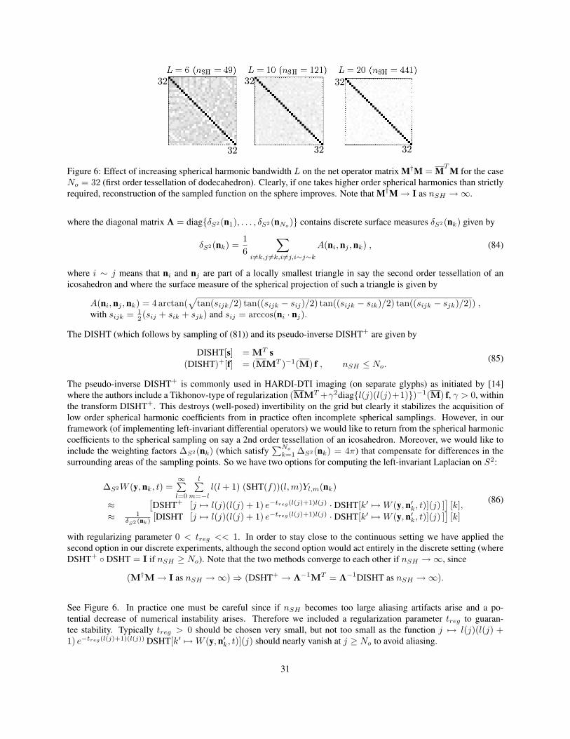
32

32

32

3232

32

Figure 6: Effect of increasing spherical harmonic bandwidth L on the net operator matrix M†M = MT M for the caseNo = 32 (first order tessellation of dodecahedron). Clearly, if one takes higher order spherical harmonics than strictlyrequired, reconstruction of the sampled function on the sphere improves. Note that M†M → I as nSH →∞.

where the diagonal matrix Λ = diagδS2(n1), . . . , δS2(nNo) contains discrete surface measures δS2(nk) given by

δS2(nk) =16

∑i 6=k,j 6=k,i6=j,i∼j∼k

A(ni, nj , nk) , (84)

where i ∼ j means that ni and nj are part of a locally smallest triangle in say the second order tessellation of anicosahedron and where the surface measure of the spherical projection of such a triangle is given by

A(ni, nj , nk) = 4 arctan(√

tan(sijk/2) tan((sijk − sij)/2) tan((sijk − sik)/2) tan((sijk − sjk)/2)) ,with sijk = 1

2 (sij + sik + sjk) and sij = arccos(ni · nj).

The DISHT (which follows by sampling of (81)) and its pseudo-inverse DISHT+ are given by

DISHT[s] = MT s(DISHT)+[f] = (MMT )−1(M) f , nSH ≤ No.

(85)

The pseudo-inverse DISHT+ is commonly used in HARDI-DTI imaging (on separate glyphs) as initiated by [14]where the authors include a Tikhonov-type of regularization (MMT +γ2diagl(j)(l(j)+1))−1(M) f, γ > 0, withinthe transform DISHT+. This destroys (well-posed) invertibility on the grid but clearly it stabilizes the acquisition oflow order spherical harmonic coefficients from in practice often incomplete spherical samplings. However, in ourframework (of implementing left-invariant differential operators) we would like to return from the spherical harmoniccoefficients to the spherical sampling on say a 2nd order tessellation of an icosahedron. Moreover, we would like toinclude the weighting factors ∆S2(nk) (which satisfy

∑No

k=1 ∆S2(nk) = 4π) that compensate for differences in thesurrounding areas of the sampling points. So we have two options for computing the left-invariant Laplacian on S2:

∆S2W (y, nk, t) =∞∑

l=0

l∑m=−l

l(l + 1) (SHT(f))(l,m)Yl,m(nk)

≈[DSHT+ [j 7→ l(j)(l(j) + 1) e−treg(l(j)+1)l(j) · DSHT[k′ 7→ W (y, n′k, t)](j) ]

][k],

≈ 1δS2 (nk) [DISHT [j 7→ l(j)(l(j) + 1) e−treg(l(j)+1)l(j) · DSHT[k′ 7→ W (y, n′k, t)](j) ]

][k]

(86)

with regularizing parameter 0 < treg << 1. In order to stay close to the continuous setting we have applied thesecond option in our discrete experiments, although the second option would act entirely in the discrete setting (whereDSHT+ DSHT = I if nSH ≥ No). Note that the two methods converge to each other if nSH →∞, since

(M†M → I as nSH →∞) ⇒ (DSHT+ → Λ−1MT = Λ−1DISHT as nSH →∞).

See Figure 6. In practice one must be careful since if nSH becomes too large aliasing artifacts arise and a po-tential decrease of numerical instability arises. Therefore we included a regularization parameter treg to guaran-tee stability. Typically treg > 0 should be chosen very small, but not too small as the function j 7→ l(j)(l(j) +1) e−treg(l(j)+1)(l(j)) DSHT[k′ 7→ W (y, n′k, t)](j) should nearly vanish at j ≥ No to avoid aliasing.

31

7.2 Finite Difference Scheme for Linear R3 o S2 Diffusion

The linear diffusion system on R3 o S2 can be rewritten as∂tW (y, n, t) =

(D11((A1)2 + (A2)2) + D33(A3)2 + D44∆S2

)W (y, n, t)

W (y, n, 0) = U(y, n) ,(87)

This system is the Fokker-Planck equation of horizontal Brownian motion on R3 o S2 if D11 = 0. Spatially, wetake second order centered finite differences for (A1)2, (A2)2 and (A3)2, i.e. we applied the discrete operators in therighthand side of (79) twice (where we replaced 2h 7→ h to ensure direct-neighbors interaction), so we have

((A3)2W )(y, n, t) ≈ W (y + hRnez, n, t)− 2 W (y, n, t) + W (y− hRnez, n, t)h2

, (88)

where one can either apply the earlier mentioned interpolation methods (2nd order B-spline or (82)) or (as we did inour experiments) one first computes all second order finite differences on the cubic spatial grid and rotates them back tothe spatial part of the moving frame of reference (26) attached to (y, n). The spherical Laplacian ∆LB is computed bymeans of (86) (second approximation). For efficiency, the chain of operators, DSHT-diagl(l+1)e−tregl(l+1)-DISHT,is stored in a single No ×No-matrix, so that calculation of ∆S2 consists of a simple matrix-vector multiplication. Inour algorithm we apply a first order approximation in time (i.e. Euler-forward scheme)

∂tW (y, n, t) ≈ W (y, n, t + ∆t)−W (y, n, t)∆t

, (89)

where we choose ∆t small enough such that the algorithm is stable. As shown in Appendix B sharp upper bounds on∆t which guarantees stability are given by

∆t ≤ minν h2

4D11+2D33, (1− ν) 2etregL(L+1)

D44L(L+1) if treg · L(L + 1) ≤ 1 ,

∆t ≤ minν h2

4D11+2D33, (1− ν) 2

D44treg e if treg · L(L + 1) > 1

(90)

where ν ∈ (0, 1) can still be freely chosen, h denotes spatial step size and L = b√

nSH − 1c. In general one hasmaxν min(νa, (1− ν)b) = ab

a+b for any a, b > 0 and thereby we attain the sharpest upper-bound

∆t ≤ h2

4D11+2D33+D44h2 L(L+1)

2 etregL(L+1)

if treg · L(L + 1) ≤ 1 ,

∆t ≤ h2

4D11+2D33+D44h2 12e treg

if treg · L(L + 1) > 1(91)

We did not take spatial second order B-spline interpolations into account11 that we used to compute (88). An increaseof spatial diffusivity and angular diffusivity yields a decrease in the maximum time step, whereas an increase of theregularity parameter treg allows a larger time step. We also recognize a turning point if treg · (L(L + 1)) = 1. Themultiplier l(j)(l(j) + 1)e−tregl(j)(l(j)+1) attains its maximum at j < nSH if treg > (L(L + 1))−1. This is desirablesince the multiplier is supposed to vanish at j = nSH ≈ No. In the experiment of Figure 10, we have set h = 10−1,no = 162, L = 18 (restricting l to even order), treg = 0.01, D33 = 1, D11 = 10−2, D44 = 10−4 and ∆t = 0.005.

7.3 Convolution Schemes for Linear R3 o S2-Diffusion

Instead of a finite difference scheme one can use the theoretical fact that the solutions of the linear diffusions (37) aregiven by R3oS2-convolution (38) with the corresponding (smooth) Green’s function pD,a

t that we derived analytically

11The interpolation has a minor effect on the stability bounds. The radius of the Gerschgorin circles associated to the spatial increments functionsget multiplied with

√2 which is the upper-bound for the cardinal B-spline, [26, p.146].

32

in Section 6. The convolution scheme is a relatively straightforward discretization of W (y, n, t) = (pD,at ∗R3oS2 U)(y)

given by (10), where the integrals are usually replaced by sums using the mid-point rule (unless one has to deal with thesingularity at the origin of the contour-completion kernel). This approach has computational advantages (in contrastto the SE(2)-convolutions) over the rather technical steerable SE(3)-convolutions [2, p.174-179]. We will return tospecific practical implementation issues, later in subsection 8.2. In this subsection we restrict ourselves to an overviewof options for the computation of the Green’s functions.

We propose the following options to evaluate the Green’s function for contour enhancement (i.e. non-zero parametersare D33 > 0, D44 = D55 > 0 and D11 = D22 ≥ 0) in the integration (38):

1. Use the finite difference scheme to numerically compute the Green’s function. Disadvantage: This requiresinterpolation. Advantage: If the time step ∆t << 1 the numeric approximation of the kernel is very accurate.

2. if D11 = D22 = 0 we can use the analytic approximation formulae for the contour enhancement kernel.Here one can either use (76) where the functions (x, n) 7→ ck(x, n) are computed by means of the algorithm(77), or one may use the simpler but less accurate formula (70) using the asymptotical formula (71). In case0 < D44/D33 << 1 one may want to use the fast Heisenberg approximation kernel (69) together with (71) .

For the contour-completion case where the non-zero parameters are a3 = 1, D44 = D55 > 0 generalizations of thefinite difference scheme of the previous section are questionable due to the trade-off between accuracy of convectionand stability of diffusion. Alternation of convection and diffusion with very small time steps (like described in [49]for the SE(2)-case) is probably preferable here. To avoid these technical issues we propose kernel-implementationsfor the contour completion case, where we distinguish between the following options:

1. For the resolvent of the contour-completion process use analytic formula (65) (accurate if 4λD44 << 1).

2. For the time-dependent contour completion process use analytical formula (66) (accurate if 4tD44 << 1).

3. For both time-dependent and resolvent contour completion process one can use the accurate (at least in theneighborhood of the z-axis) relation (107) (in the spatial Fourier domain) to contour-completion on SE(2),together with earlier developed algorithms [6, 7, 49, 20, 23] for contour completion on SE(2).

Figure 7 shows HARDI-glyph visualizations of several contour enhancement kernels and Figure 8 shows HARDI-glyph visualizations of a contour completion kernel.

8 Experiments of Linear Crossing-preserving Diffusion on HARDI images

In the previous section we have discussed two different kinds of implementations of crossing-preserving diffusionon HARDI images, namely left-invariance finite difference schemes and left-invariant convolution schemes. In thissection we will show some experiments of these approaches and furthermore we discuss some practical issues thatcome along with these approaches.

Before we will consider the different practical properties of the two approaches, we briefly comment on their analogies.Firstly, each step in the finite difference schemes is a linear kernel operator and thereby in principle (due to Corollary 1)a R3oS2-convolution with a small kernel which is non-zero on the discretization stencil). Secondly, the computationalorder of the algorithms is comparable. The R3oS2-convolutions are of order O(NsN0KsKo) and the finite differenceschemes are of order O(NsNoNitNst), where Ns, No respectively stands for the total number of spatial and orientationsamples of the HARDI-image, Ks,Ko respectively stand for the number of spatial samples and average number of

33

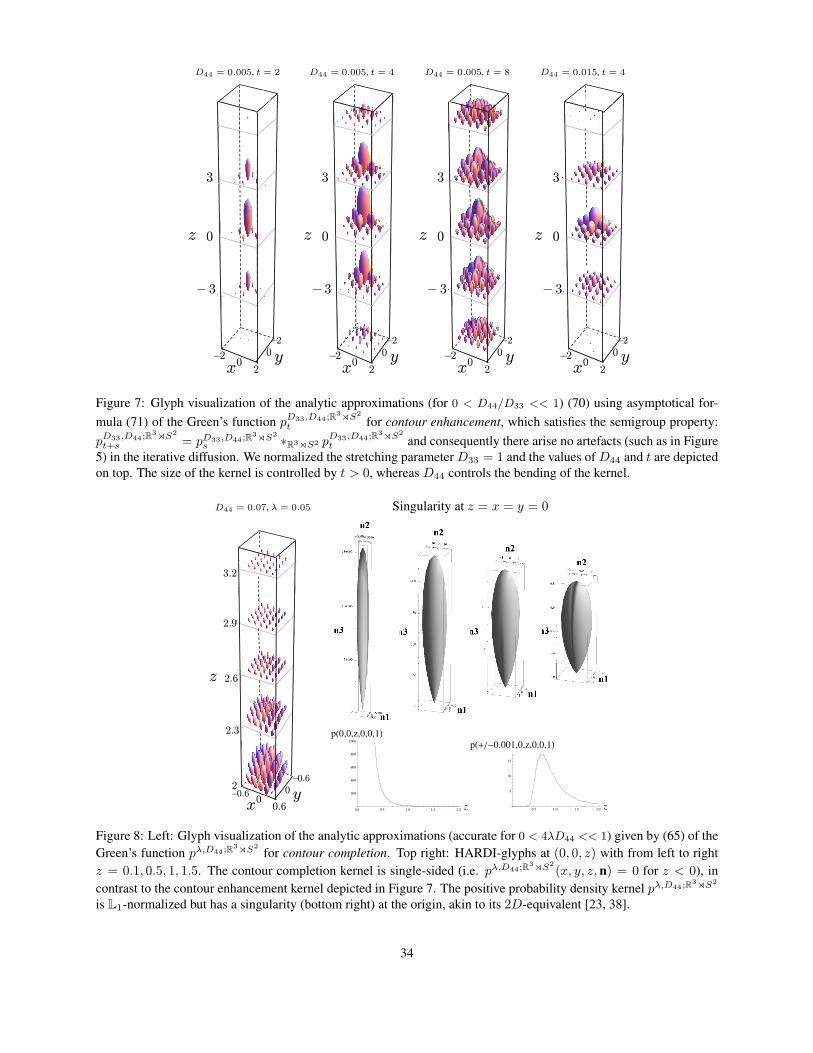
D44 = 0.005, t = 2 D44 = 0.005, t = 4 D44 = 0.005, t = 8 D44 = 0.015, t = 4

2

0−2

− 3

0

−2

z

xy

0

3

0

3

2

0−2

− 3

0

−2

z

xy

3

−2

− 3

z 0

2

00

−2

xy

3

2

0−2

− 3

0

−2

z

xy

0

Figure 7: Glyph visualization of the analytic approximations (for 0 < D44/D33 << 1) (70) using asymptotical for-mula (71) of the Green’s function pD33,D44;R3oS2

t for contour enhancement, which satisfies the semigroup property:pD33,D44;R3oS2

t+s = pD33,D44;R3oS2

s ∗R3oS2 pD33,D44;R3oS2

t and consequently there arise no artefacts (such as in Figure5) in the iterative diffusion. We normalized the stretching parameter D33 = 1 and the values of D44 and t are depictedon top. The size of the kernel is controlled by t > 0, whereas D44 controls the bending of the kernel.

D44 = 0.07, λ = 0.05 Singularity at z = x = y = 0

z

0 y

2.6

2.3

2

2.9

3.2

0x−0.6

0.6

−0.6

Out[93]=

Out[86]=

0.0 0.5 1.0 1.5 2.0 z

200

400

600

800

1000

pH0,0,z,0,0,1L

0.5 1.0 1.5 2.0 z

5

10

15

pH+ê-0.001,0,z,0,0,1L

Out[86]=

0.0 0.5 1.0 1.5 2.0 z

200

400

600

800

1000

pH0,0,z,0,0,1L

0.5 1.0 1.5 2.0 z

5

10

15

pH+ê-0.001,0,z,0,0,1L

Figure 7: Bla

33

Figure 8: Left: Glyph visualization of the analytic approximations (accurate for 0 < 4λD44 << 1) given by (65) of theGreen’s function pλ,D44;R3oS2

for contour completion. Top right: HARDI-glyphs at (0, 0, z) with from left to rightz = 0.1, 0.5, 1, 1.5. The contour completion kernel is single-sided (i.e. pλ,D44;R3oS2

(x, y, z, n) = 0 for z < 0), incontrast to the contour enhancement kernel depicted in Figure 7. The positive probability density kernel pλ,D44;R3oS2

is L1-normalized but has a singularity (bottom right) at the origin, akin to its 2D-equivalent [23, 38].

34

orientation samples of the convolution kernel and Nit stands for number of iteration with a discretization stencil oflength Nst. Thirdly, both approaches are very well suited for parallel implementation.

8.1 Experiments Finite Difference Scheme

We implemented linear, left-invariant diffusion on HARDI data with diagonal diffusion matrix D = diag(Dii) withD11 = D22, D44 = D55 (and D66=0) using an explicit numerical scheme as explained in Subsubsection 7.2. Figure9 and 10 show results of the linear diffusion process. In these examples an artificial three-dimensional HARDI datasetis created, to which Rician noise is added, meaning that we applied the transformation

( (y, n) 7→ U(y, n) ) 7→ ( (y, n) 7→√

(U(y, n) cos(η1) + η2)2 + (U(y, n) sin(η1) + η3)2 ) (92)

where η2, η3 ∼ N (0, σ) normally distributed and η1 uniformly distributed over [0, 2π).

Next, we applied two different R3 o S2-diffusions on both the noise-free and the noisy dataset. To visualize ourresults we used the DTI tool (see http://www.bmia.bmt.tue.nl/software/dtitool/ ) which can visualize HARDI glyphsusing the Q-ball visualization method [14]. In the results, all glyphs are scaled equivalently. The isotropic diffusion(D33 = D22 = D11) does not preserve the anisotropy of the glyphs well; especially in the noisy case we observe thatwe get almost isotropic glyphs. With anisotropic diffusion, the anisotropy of the HARDI glyphs is preserved muchbetter and in the noisy case the noise is clearly reduced. See Figures 9 and 10. The resulting glyphs are, however,less directed than in the noise-free input image. This would improve when using nonlinear diffusion. The basictheoretical PDE-framework for non-linear diffusions, is the subject of the last section. As an alternative to non-linearadaptive diffusion, we are currently investigating the inclusion of sharpening steps by means of left-invariant erosions(solutions of left-invariant Hamilton-Jakobi PDE’s on HARDI data). Practical properties of the left-invariant finitedifference schemes:

++ It is relatively easy to adapt and generalize to non-linear (adaptive) diffusion schemes.−− The explicit finite difference scheme is only stable for sufficiently small time steps.− The algorithm includes extra numerical blur, which does not accurately follow the continuous PDE-theory.− If the DSHT-coefficients of the initial HARDI-set quickly decay one obtains best results with a small treg > 0.

But often for those values of treg the corresponding impulse response contains aliasing artefacts.

8.2 Implementation and Experiments Convolution Schemes

In Subsection 7.3 we have provided an overview of options for computing the Green’s functions of contour enhance-ment and contour completion. Now suppose we have chosen an analytic approximation formula p(y, n) for the Green’sfunction p : R3 o S2 → R+, then we can rewrite (38) in L2-inner product form

(p ∗R3oS2 U)(y, n) = (L(y,Rn)p, U)L2(R3oS2), (93)

where we recall Definition 2 of L and where we define p(y′, n′) := p(−RTn′y′, RT

n′ez). Note that

p(y′, n′) = k(0, ez ; y′, n′) and p(y, n) = k(y, n ; 0, ez), for all (y, n), (y′, n′) ∈ R3 o S2.

Now p(y, n) denotes the probability density of finding a random walker at (y, n) given that it started at (0, ez), so thatp(y, n) = p(−RT

n y, RTn ez) denotes the probability density of finding a random walker at (−RT

n y, RTn ez) given that it

started at (0, ez), which is by left-invariance of the stochastic process the same as the probability density of finding arandom walker at (0, ez) given that it started at (y, n).

The main advantage of formula (93) is that in practice we can pre-compute/sample all rotated versions and translatedversions L(y,Rn)p | y ∈ R3, n ∈ S2 of the check-kernel p, so that the remainder of the algorithm just consists of

35

194 Chapter 7. 3D Orientation Scores

(a) t = 0, no noise (b) t = 0, added noise

(c) t = 1, µ-isotropic, no noise (d) t = 1, µ-isotropic, added noise

(e) t = 1, anisotropic, no noise (f) t = 1, anisotropic, added noise

Figure 7.9: Result of R3 o S2-diffusion on an artificial HARDI dataset of two crossinglines, with and without added Rician noise with σ = 0.17 (signal amplitude 1). Imagesize: 10 × 10 × 10 spatial and 162 orientations. Parameters of the µ-isotropic diffusionprocess: Da = 1, µ = 0.1, treg = .01. Parameters of the anisotropic diffusion process:Da = 0.01, µ = 0.1, treg = .01.

Figure 9: Result of R3 o S2-diffusion (computed by the finite difference scheme, section 7.2) on an artificial HARDIdataset of two crossing straight lines, with and without added Rician noise (92) with σ = 0.17 (signal amplitude 1).Image size: 10× 10× 10 spatial and 162 orientations. Parameters of the isotropic diffusion process: D11 = D22 =D33 = 1, D44 = D55 = 0.01. Parameters of the anisotropic diffusion process: D11 = D22 = 0.01, D33 = 1, D44 =D55 = 10−4. In both cases we have set treg = 0.01 in (82).

36

(a) t = 0 no noise (b) t = 0 added noise

(c) t = 1 no noise (d) t = 1 added noise

Figure 10: Result of R3 oS2-diffusion (computed by the finite difference scheme, section 7.2) on an artificial HARDIdataset of two crossing lines where one of the lines is curved, with and without added Rician noise (92) with σ = 0.17(signal amplitude 1). We have magnified the crossing areas on the top-right of the figures before and after the linearanisotropic diffusion. Image size: 10× 10× 10 spatial and 162 orientations. Parameters of the linear anisotropicdiffusion process: D11 = D22 = 0.01, D33 = 1, D44 = D55 = 10−4 and treg = 0.01 in (82).

37

computing L2-inner products which can be done in parallel. In contrast to the finite difference schemes, the convolutionschemes are unconditionally stable. In fact we even have

‖p ∗R3oS2 U‖L1(R3oS2) = ‖p‖L1(R3oS2)‖U‖L1(R3oS2) = 1 · ‖U‖L1(R3oS2) ,‖p ∗R3oS2 U‖L∞(R3oS2) = sup

(y,n)|p ∗R3oS2 U(y, n)| ≤ ‖L(y,Rn)p‖L2(R3oS2)‖U‖L2(R3oS2) ≤ ‖p‖L2(R3oS2)‖U‖L2(R3oS2).

i.e. preservation of mass (which also holds on the discrete grid if the discretely sampled versions of L(y,Rn)p are`1-normalized on the grid) and a small L2-pertubation on the input yields a small L∞-pertubation on the output.

Finally, formula (93) provides the following fast discrete approximation/truncation:

(p ∗R3oS2 U)(y, n) ≈∑

y′∈R3, ‖y′−y‖∞≤R

K(y′,y,n)∑k=1

(Ly,Rn p)(y′, n′k(y′, y, n))∆y′ δS2(n′k), (94)

with spatial step size ∆y = (∆y′1,∆y′2,∆y′3) and where we truncated the spatial integration to a cube ‖y′ − y‖∞ =sup

i=1,2,3|y′i− yi| ≤ R, R > 0, where we recall (84) and where nk(y′, y, n)No

k=1, forms an a priori defined lookup table

by sorting the points nkNo

k=1 such that

L(y,Rn)p(y′, nk+1) < L(y,Rn)p(y′, nk)

and where K(y′, y, n) = maxk ∈ 1, . . . , No | L(y,Rn)p(y′, nk) ≤ ε, with tolerance ε > 0. We usually setR ∈ 1, 2, 3, 4 (see for example Figure 11 where we even set R = 1) for the spatial truncation and ε = 10−5

for angular truncation. The gain in speed mostly lies in the angular truncation, as the convolution kernels are forreasonable parameter settings of D33, D44, t, λ rather orientation-selective, recall Figure 7 and Figure 8.

Summarizing we have the following practical properties of the left-invariant convolution schemes:

+ The convolution kernels can be pre-computed and truncated.+ The algorithm does not suffer from the typical numerical blur of finite difference schemes.

+ + The algorithm is unconditionally stable.+ For single sided kernels (completion) one can include reflections, as we will see in Subsection 8.2.1.

+ + The algorithm is easily extended to left-invariant dilations/erosions on HARDI images by replacing the(+, ·)-algebra by the (max,+)-algebra in the convolution, akin to previous work on regular images [9, 10].

- - Generalization to non-linear adaptive diffusions: Adapting the kernel to the data locally is no longer a convolutionand the relation to left-invariant PDE’s is no longer clear.

8.2.1 Spherical Reflection Symmetries: Preservation of Reflection Symmetry in Contour Enhancement andincluding Glyph-attraction in Contour Completion

The big difference between the stochastic processes for contour completion and contour enhancement is that contourcompletion kernels (Green’s functions) are single-sided, whereas contour enhancement kernels (Green’s functions) aredouble-sided. Compare Figure 7 to Figure 8. This change in reflection symmetry has two consequences:

1. The initial HARDI-data are usually invariant under spherical reflections, i.e. U(y, n) = (rS2U)(y, n) :=U(y,−n). In contrast to contour completion, contour enhancement preserves this symmetry during the evo-lution, as can be seen in Figure 9 and Figure 10. This directly follows by the fact that the generator of contourcompletion −A3 + ∆S2 and the generator of contour enhancement (A3)2 + ∆S2 satisfy

(−A3 + ∆S2) rS2 = rS2 (+A3 + ∆S2) ,((A3)2 + ∆S2) rS2 = rS2 ((A3)2 + ∆S2) .

(95)

38

2. It allows a relevant extension of our contour completion processes, where we replace the R3 o S2-convolutionsby (R3 o O(3))/(0 × SO(2)) convolutions as we will explain next. The practical advantage of these (R3 oO(3))/(0×SO(2))-convolution is that it allows us to include attraction of glyphs, rather than continuation ofglyphs. See Figure 11 and compare the two images in the middle. To achieve this extension we need a differentkind of reflections, namely spatial reflections given by rR3U(y, n) := U(−y, n). These spatial reflections rR2

intertwine the contour enhancement and completion generators in the same way as the angular reflections rS2 :

(−A3 + ∆S2) rR3 = rR3 (+A3 + ∆S2) ,((A3)2 + ∆S2) rR3 = rR3 ((A3)2 + ∆S2) .

(96)

Now indeed (96) is analogous to (95) but the crucial difference between these two types of reflections is:

rR3δe = δe and rS2δe 6= δe and rR3U 6= U and rS2U = U . (97)

Now (97) and (96) directly imply the spatial reflection symmetry of the contour enhancement kernel as can beseen in Figure 7. Clearly the contour completion kernel does not admit such a symmetry and we arrive at thefollowing three possible choices of (R3 o O(3))/(0×SO(2))-convolutions for the contour completion case:

(pλ,D44 ∗(R3oO(3))/(0×SO(2)) U)(y, n) =P

ε′∈−1,1qab(ε

′)R

S2

RR3

pλ,D44(ε′ RTn′(y− y′), RT

n′n) U(y′, n′) dy′dσ(n′)

with qab(ε′) = 1

2(a δε′ 1 + b δ−ε′ 1) , a, b ∈ 0, 1, ab 6= 0.

(98)

These two issues are illustrated in Figure 11 for a simple example of a HARDI-image induced by a DTI-image, i.e.

U(y, n) = nT D(y)n (99)

In Figure 11 we have set rotation matrices S(y) such that D(y) = (S(y))−1diag0.1, 0.1, 1S(y). Furthermore, weapplied Rician noise on the HARDI-data, recall (92). The particular case a = b = 1 in (98) yields results that aresimilar to convolution with contour enhancement kernels (recall Figure 7) for suitable choice of D33 and D44. Thedifference in practice is that the sum of two spatially reflected contour completion kernels yields a double sided kernelthat is typically sharper kernel at the center than a contour enhancement kernel, as can be observed by comparing thesecond and fourth image in the bottom row of Figure 11.

We conclude from Figure 11 that in the case of 1-sided kernels and a = 0 and b = 1 glyphs attract each other, providedthat the initial HARDI-data set has an antipodal symmetry (i.e. is invariant under rS2). In the case of 1-sided kernelsand (a = 1, b = 1) we obtain a 2-sided kernel which preserves the antipodal symmetry. The output for such caseis comparable to the enhancement case (again preserving antipodal symmetry), with the difference that the contourenhancement kernel is less sharp at the center and therefore includes more directional information from the side.

9 Non-Linear, Adaptive, Left-Invariant Diffusions on HARDI images

So far we have considered linear left-invariant diffusions, whose solutions are given by convolution with a fixedGreen’s function reflecting an a priori probability model for fiber-extension. In many applications however, it isimportant to adapt the fiber-extension model to the data, where we can include adaptive curvature and adaptive torsion.Now by Theorem 3, it follows that in order to include adaptive torsion and curvature we must re-align the left-invariantlocal coordinate frame A1, . . . ,A5 by means of a locally optimally fitting exponential curve, where we recall (52)).

Our first aim is to determine the exponential curve (55) that optimally fits the distribution (y, n) 7→ U(y, n) ∈ R+ ateach position (y, n) ∈ R3oS2. Recall that such a distribution gives rise to a probability distribution (x, R) 7→ U(x, R)on SE(3) by means of (28). To achieve our goal, we follow the same approach as in our previous works on non-lineardiffusions on invertible orientation scores (of 2D-images) defined on SE(2) [26, p.118-120], [21, ch:3.4], [27, ch:5.2].

39

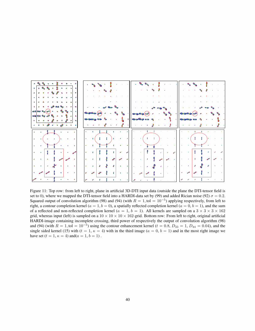
Figure 11: Top row: from left to right, plane in artificial 3D-DTI input data (outside the plane the DTI-tensor field isset to 0), where we mapped the DTI-tensor field into a HARDI-data set by (99) and added Rician noise (92) σ = 0.2.Squared output of convolution algorithm (98) and (94) (with R = 1, tol = 10−5) applying respectively, from left toright, a contour completion kernel (a = 1, b = 0), a spatially reflected completion kernel (a = 0, b = 1), and the sumof a reflected and non-reflected completion kernel (a = 1, b = 1). All kernels are sampled on a 3 × 3 × 3 × 162grid, whereas input (left) is sampled on a 10× 10× 10× 162-grid. Bottom row: From left to right, original artificialHARDI-image containing incomplete crossing, third power of respectively the output of convolution algorithm (98)and (94) (with R = 1, tol = 10−5) using the contour enhancement kernel (t = 0.8, D33 = 1, D44 = 0.04), and thesingle sided kernel (15) with (t = 1, κ = 4) with in the third image (a = 0, b = 1) and in the most right image wehave set (t = 1, κ = 4) and(a = 1, b = 1) .

40

We again formulate a minimization problem that minimizes over the “iso-contours” of the left-invariant gradient vectorat (y, n) ∈ R3 o S2, yielding optimal tangent vector c∗(y, n) = (c1

∗(y, n), . . . , c5∗(y, n), 0)T :

c∗(y, n) = arg minc(y,n)

∥∥∥∥∥ d

dt(∇U(g etc(y,n)))

∣∣∣∣∣t=0

∥∥∥∥∥2

µ

∣∣∣∣ ‖c(y, n)‖µ = 1

, (100)

where the left-invariant gradient dU =5∑

i=1

Ai(U) dAi, a co-vector, is represented by row-vector given by

∇U = AU = (A1U , . . . ,A5U , 0).

where ‖·‖µ denotes both the norm on a vector in tangent space Tg(SE(3)) (i.e. the norm at the right side) and the dualnorm on a covector in the dual tangent space T ∗g (SE(3)) (the norm on the left side). We represent tangent vectors

c(y, n) =5∑

i=1

ci(y, n) Ai|g=(y,Rn)

as column-vector c(y, n) = (c1∗(y, n), . . . , c5

∗(y, n), 0)T and their norm is defined by ‖c‖µ :=√

(c, c)µ with the inner

product (c, c)µ := µ2(∑3

j=1 cjcj)

+∑6

j=4 cjcj . where parameter12 µ (with physical dimension 1/[length]) ensuresthat all components of the inner product are dimensionless. The value of the parameter determines how the distancein the spatial dimensions relates to distance in the orientation dimension. Implicitly, this also defines the norm oncovectors by ‖c‖µ =

√(c, c)µ, (c, c)µ = 〈c, G−1

µ c〉 = µ−2(∑3

j=1 cjcj) +∑6

j=4 cjcj . By means of the calculus ofvariations it follows that the minimizer c∗(y, n) satisfies

(MµHU(g)Mµ)T (MµHU(g)Mµ) c∗(y, n) = λ c∗(y, n), (101)

where Mµ := diag(1/µ, 1/µ, 1/µ, 1, 1, 1) and c∗ = M−1µ c∗ and where the 6×6 Hessian of U on R3 oS2 is given by

HU(g) = [AjAiU(g)]i row-indexj column index, g = (y, R) ∈ SE(3).

where the last row contains of zero’s only. This amounts to eigensystem analysis of the symmetric 6 × 6 matrix-valued function g 7→ (MµHU(g)Mµ)T (MµHU(g)Mµ), where one of the three eigenvectors gives c∗(y, n). Theeigenvector with the smallest corresponding eigenvalue is selected as tangent vector c∗(y, n), and the desired tangentvector c∗(y, n) is then given by c∗(y, n) = Mµ c∗(y, n).

Now that we have computed the optimal tangent vector c(y, n) at (y, n) 7→ U(y, n) (and thereby the best fittingexponential curve t 7→ g e

P5i=1 ciAi in R3 o S2) we construct the non-linear adaptive diffusion function as follows:

D(U)(y, n) = c∗(y, n)c(y, n)T µ2(1−Da(U)(y, n))‖c(y, n)‖2µ

+ Da(U)(y, n)(

I3 00 µ2I3

),

where Da(U)(y, n) is a locally adaptive anisotropy factor. Finally, we note that the conditions (34) are satisfied so ourfinal well-defined non-linear diffusion system on the HARDI data are:

∂tW (y, n, t) = (Ai [D(U)(y, n)]ij Aj W )(y, n, t) ,limt↓0

W (y, n, t) = U(y, n) . (102)

12In some of our previous works on SE(2) we denoted this fundamental parameter by β−1 > 0, but here we use µ > 0 to avoid confusion withEuler-angle β > 0 in SO(3). The left-invariant metric on SE(3) is given by the first fundamental form

P3i=1 µ2dAi⊗dAi+

P6j=4 dAj⊗dAj .

41

10 Conclusion

For the purpose of tractography (detection of biological fibers) and visualization, DTI and HARDI data should beenhanced such that fiber junctions are maintained, while reducing high frequency noise in the joined domain R3 o S2

of positions and orientations. Therefore we have considered diffusions on HARDI and DTI induced by fundamentalstochastic processes on R3 o S2 embedded in the group manifold SE(3) of 3D-rigid body motions. We have shownthat the processing must be left-invariant and we have classified all linear left-invariant diffusions on HARDI images.We presented two novel diffusion approaches which take place simultaneously over both positions and orientations.These two approaches do allow enhancement of fibres while preserving crossings and/or bifurcations. These twodiffusions are Fokker-Planck equations of stochastic processes (random walks) for respectively contour enhancementand contour completion. In a contour completion process a random walker always proceeds forward in space along itsprescribed random direction, whereas in a contour enhancement process the random walker randomly moves forwardand backward in its prescribed random orientation. As a result the contour completion process is generated by −A3 +D44∆S2 whereas the contour enhancement process is generated by the sub-Laplacian +D33(A3)2 + D44∆S2 , withD33, D44 > 0 and ∆S2 |H = A2

4 + A25 the Laplace-Beltrami operator on the sphere and where Ai-denotes the i-th

left-invariant vector field on R3 oS2. Consequently, the contour enhancement process preserves the angular reflectionsymmetry of HARDI data, whereas the contour completion process allows a choice between attraction or continuationof glyphs.

As the solutions of linear left-invariant diffusion equations are given by R3 o S2-convolution with their Green’sfunctions, we arrive at two types of implementations: Convolution schemes and finite difference schemes. Practicaladvantages of convolution schemes over finite difference schemes for linear diffusions are: they are unconditionallystable and do not involve the typical numerical blurring of a finite difference scheme. However, the finite differenceschemes with sufficiently small time steps do provide crossing preserving diffusion as well, and they are preferablefor our extensions to non-linear adaptive diffusions proposed in Section 9.

The crucial theoretical observations in our framework lie in the fact that the left-invariant evolution equations areexpressed by a quadratic form in the left-invariant vector fields Ai6i=1 on R3 o S2 embedded in SE(3), whichform a moving frame of reference consisting of a spatial velocity part A1,A2,A3 and an angular velocity partA4,A5,A6. This moving frame of reference requires the Cartan connection viewpoint13 on the underlying differ-ential geometry and by expressing the left-invariant diffusions in covariant derivatives we see that even the adaptivenon-linear left-invariant evolutions locally take place along the covariantly constant curves, which coincide with theexponential curves in SE(3). The spatial part of the exponential curves are circular spirals, i.e. curves in R3 withconstant curvature and constant torsion. As a result our non-linear adaptive diffusion schemes allow adaptation forcurvature and torsion.

The general theory and results in this article apply to any engineering application where enhancement of (possiblycrossing and/or bifurcating) fibers is required given an initial probability distribution on 3D-positions and orientations.

Acknowledgements.

Vesna Prckovska en Paulo Rodriguez, biomedical image analysis group Eindhoven University of Technology aregratefully acknowledged for providing the artificial HARDI test images and the DTI tool supporting HARDI glyphs.Special thanks to Mark Bruurmijn and Paulo Rodriguez, Eindhoven University of Technology, for their support onthe visualization and implementation of R3 o S2-convolutions. The Netherlands Organization for Scientific Research(NWO) is gratefully acknowledged for financial support.

13Rather than the torsion free Levi-Cevita connection on the Riemannian manifold (SE(3), (diag(µ2, µ2, µ2, 1, 1, 1))ij dAi ⊗ dAj).

42

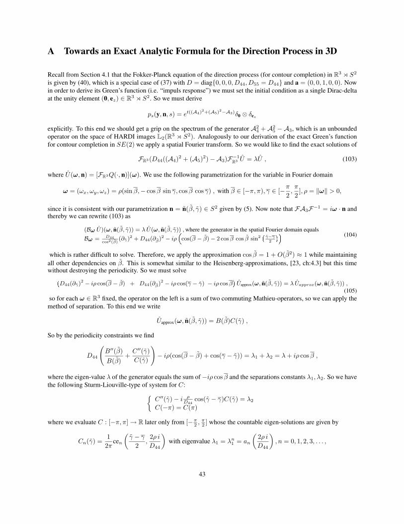
A Towards an Exact Analytic Formula for the Direction Process in 3D

Recall from Section 4.1 that the Fokker-Planck equation of the direction process (for contour completion) in R3 o S2

is given by (40), which is a special case of (37) with D = diag0, 0, 0, D44, D55 = D44 and a = (0, 0, 1, 0, 0). Nowin order to derive its Green’s function (i.e. “impuls response”) we must set the initial condition as a single Dirac-deltaat the unity element (0, ez) ∈ R3 o S2. So we must derive

ps(y, n, s) = et((A4)2+(A5)

2−A3)δ0 ⊗ δez

explicitly. To this end we should get a grip on the spectrum of the generator A24 +A2

5 − A3, which is an unboundedoperator on the space of HARDI images L2(R3 o S2). Analogously to our derivation of the exact Green’s functionfor contour completion in SE(2) we apply a spatial Fourier transform. So we would like to find the exact solutions of

FR3(D44((A4)2 + (A5)2)−A3)F−1R3 U = λU , (103)

where U(ω, n) = [FR3Q(·, n)](ω). We use the following parametrization for the variable in Fourier domain

ω = (ωx, ωy, ωz) = ρ(sinβ,− cos β sin γ, cos β cos γ) , with β ∈ [−π, π), γ ∈ [−π

2,π

2], ρ = ‖ω‖ > 0,

since it is consistent with our parametrization n = n(β, γ) ∈ S2 given by (5). Now note that FA3F−1 = iω · n andthereby we can rewrite (103) as

(Bω U)(ω, n(β, γ)) = λ U(ω, n(β, γ)) , where the generator in the spatial Fourier domain equals

Bω = D44cos2(β)

(∂γ)2 + D44(∂β)2 − iρcos(β − β)− 2 cos β cos β sin2

γ−γ

2

(104)

which is rather difficult to solve. Therefore, we apply the approximation cos β = 1 + O(β2) ≈ 1 while maintainingall other dependencies on β. This is somewhat similar to the Heisenberg-approximations, [23, ch:4.3] but this timewithout destroying the periodicity. So we must solve

D44(∂γ)2 − iρ cos(β − β) + D44(∂β)2 − iρ cos(γ − γ) − iρ cos βUapprox(ω, n(β, γ)) = λ Uapprox(ω, n(β, γ)) ,

(105)so for each ω ∈ R3 fixed, the operator on the left is a sum of two commuting Mathieu-operators, so we can apply themethod of separation. To this end we write

Uapprox(ω, n(β, γ)) = B(β)C(γ) ,

So by the periodicity constraints we find

D44

(B′′(β)B(β)

+C ′′(γ)C(γ)

)− iρ(cos(β − β) + cos(γ − γ)) = λ1 + λ2 = λ + iρ cos β ,

where the eigen-value λ of the generator equals the sum of−iρ cos β and the separations constants λ1, λ2. So we havethe following Sturm-Liouville-type of system for C:

C ′′(γ)− i ρD44

cos(γ − γ)C(γ) = λ2

C(−π) = C(π)

where we evaluate C : [−π, π] → R later only from [−π2 , π

2 ] whose the countable eigen-solutions are given by

Cn(γ) =12π

cen

(γ − γ

2,2ρ i

D44

)with eigenvalue λ1 = λn

1 = an

(2ρ i

D44

), n = 0, 1, 2, 3, . . . ,

43

where the function q 7→ an(q) denotes the Mathieu-characteristics, [42, 1] and where cen(·, q) denotes the cosineelliptic Mathieu-function (with Floquet exponent n), [42, 1], which is a π-periodic solution of Mathieu’s equationy′′(z) + 2 q cos(2z)y(z) = an(q)y(z). Similarly, the eigensystem of

B′′(β)− i ρD44

cos(β − γ)B(β) = λ1

B(−π) = B(π)

is given by Bm(β) = 12π

cem

β−β

2, 2ρ i

D44

with eigenvalue λm

1 = am

2ρ iD44

, m = 0, 1, 2, 3, . . . ,. Consequently, a com-

plete set of bi-orthogonal14 eigenfunctions (with eigen values λmn) of the generator Bω is given by

Umn(ω, n(β, γ)) =cen

γ−γ

2 , 2ρD44

cen

β−β

2 , 2ρD44

4π2 and λmn(ω) = −iρ cos β −

am

2ρ iD44

+an

2ρ iD44

4 < 0.

Consequently, we have the following approximation formula for pD44=D55,a3=1s = FR3pD44=D55,a3=1

s :

FR3

e

t((A4)2+(A5)2−A3)|cos β=1δ0 ⊗ δez

(ω, n(β, γ)) =

∞Xm=0

∞Xn=0

et λmn(ω)Umn(ω, n(β, γ))Umn(0, n(β, γ)). (106)

Now this expression is quite similar to one of our exact formulas for the (spatial) Fourier transform FR2pSE(2),D44t

of the Green’s function pSE(2),D44t : (SE(2)\e) → R+ of the direction process in SE(2). In fact we have the

following intriguing geometrical relation

FR3

et((A4)2+(A5)2−A3)δ0 ⊗ δez

(ω, n(β, γ)) ≈ FR3

e

t((A4)2+(A5)2−A3)|cos β=1δ0 ⊗ δez

(ω, n(β, γ)) =

= e−iRt(FR2pSE(2),D44t )

ωzρR

,−ωyρ

R, eiγ

(FR2p

SE(2),D44t )

R, ωx, eiβ

,

(107)

with ρ =√

ω2x + ω2

y + ω2z and R :=

√ω2

y + ω2z , which allows us to use efficient algorithms [23, 6] for the compu-

tation of the Green’s function of the contour completion process in SE(2) for the computation of the approximation(107) of the Green’s function of the contour completion process in SE(3).

B Stability and Step Size of the Finite Difference Scheme

In this section we will derive the upper bound for the step size (90) that guarantees the stability of the finite differencescheme explained in Subsection 7.2.

We shall use (88) and (89) as starting point for our Euler-forward discretization of evolution (87). For each q ∈ N∪0,we define the vector wq = (wq

y,k)k=1...No,y∈I , where k enumerates the number of samples on the sphere, wherey enumerates the samples on the discrete spatial grid I = 1, . . . , N × 1, . . . , N × 1, . . . , N and where qenumerates the discrete time frames. Rewrite (88) and (89) in vector form

wq+1 = (I −∆t(JS2 + JR3))wq ,

where the angular increments block-matrix equals

JS2 = 0⊕D44Λ−1MT QMΛ ∈ R(3N+No)×(3N+No), with Q = diagQjj = diagl(j)(l(j)+1)e−tregl(j)(l(j)+1),

14Here bi-orthogonality means that the conjugation is omitted in the L2inner-product, i.e.R π

−π

R 2π

0Um′n′(β, γ)Umn(β, γ)dγdβ =

Um′n′ , Umn

L2([−π,π]×[0,2π])

= δmm′δnn′ , which follows from the fact that (Bω)∗φ = Bωφ for all φ ∈ H2([−π, π]× [0, 2π]).

44

according to the second approach in (86) and where the spatial increments block matrix equals

JR3 = h−2(D11B1 ⊕D11B2 ⊕D33B3) ⊕ 0 ∈ R(3N+No)×(3N+No)

with spatial stepsize h and Bi ∈ RN×N standard sparse 3-band matrices associated to stencil (−1, 2,−1) with cyclicboundary conditions, according to (88). Both JS2 and JR3 are positive semi-definite. We have guaranteed stability iff

‖I −∆t(JS2 + JR3)‖ = sup‖w‖=1‖(I −∆t(JS2 + JR3))w‖ < 1,

which is by I −∆t(JS2 + JR3) = (νI −∆tJR3) + ((1− ν)I −∆tJS2), with ν ∈ (0, 1), the case if

‖I − ∆t

νJR3‖ < 1 and ‖I − ∆t

1− νJS2‖ < 1 ⇒ ‖(νI −∆tJR3)+ ((1− ν)I −∆tJS2)‖ < ν +(1− ν) = 1. (108)

Sufficient (and sharp) conditions for the first inequality are obtained by means of the Gerschgorin Theorem [29] :

∆t ≤ νh2

4D11 + 2D33. (109)

Sufficient and sharp conditions for the second equality are obtained by considering the spectrum σ(I − 11−ν ∆tJS2)

of symmetric matrix I − 11−ν ∆tJS2 and by M†M ≈ I (recall Figure 6) and M†M → I as nSH →∞ we have

σ(I − 11−ν ∆tJS2) = σ(I − 1

1−ν D44 ∆t Λ−1MT QMΛ)→ σ(I − 1

1−ν D44∆t Q) as nSH →∞.(110)

Now in general σ(I − 11−ν ∆tJS2) ≈ σ(I − 1

1−ν D44∆t Q) and thereby the spectrum is contained in (−1, 1) iff

∆t ≤ 2(1−ν)D44max(Qjj)

where the maximum of the diagonal elements Qjj equals

max(Qjj) =

L(L + 1)e−tregL(L+1) if treg · L(L + 1) < 1(e treg)−1 else

(111)

since 0 < x 7→ xe−tregx attains its only maximum at x = 1treg

. Now (108), (109), (110) and (111) imply result (90).

References[1] M. Abramowitz and I. A. Stegun, editors. Handbook of Mathematical Functions with Formulas, Graphs, and Mathematical

Tables. Dover Publications, Inc., New York, 1965. Originally published by the National Bureau of Standards in 1964.

[2] M. A. van Almsick. Context Models of Lines and Contours. PhD thesis, Eindhoven University of Technology, Department ofBiomedical Engineering, Eindhoven, The Netherlands, 2005. ISBN:978-90-386-1117-4.

[3] L. Alvarez and F. Guichard, F. and P. L. Lions and J.-M. Morel. Axioms and Fundamental Equations of Image Processing.Arch. Rat. Mech. Anal. , (123):200–257, 1993.

[4] V.Arsigny, X. Pennec and N. Ayache. Bi-invariant Means in Lie Groups. Application to Left-invariant Polyaffine Transfor-mations. Technical report, nr. 5885, INRIA, France, April 2006.

[5] T. Aubin. A Course in Differential Geometry Graduate Studies in Mathematics, AMS, Vol. 27, 2001.

[6] J. August. The Curve Indicator Random Field. PhD thesis, Yale University, 2001.

[7] J. August and S.W. Zucker. The curve indicator random field and markov processes. IEEE-PAMI, Pattern Recognition andMachine Intelligence, 25, 2003. Number 4.

[8] A. Barmpoutis and B.C. Vemuri and D. Howland and J.R. Forder Extracting Tractosemas from a Displacement ProbabilityField for Tractography in DW-MRI. Proc. MICCAI 2008, part I, Springer-Verlag, Lecture Notes Computer Science 5241, p.9–16, 2008.

45

[9] B. Burgeth and J. Weickert An Explanation for the Logarithmic Connection between Linear and Morphological Systems.Lecture Notes in Computer Science, Proc. 4th int. Conference Scale Space 2003, SpringerVerlag, 2003, p. 325–339.

[10] B. Burgeth and M.Breuss and S.Didas and J.Weickert PDE-based Morphology for Matrix Fields: Numerical Solution SchemesTechnical Report No. 220, Math. and Comp. Science, Saarland University, Saarbrucken 2008.

[11] A.V. Bukhvalov and W. Arendt. Integral representation of resolvent and semigroups. Forum Math. 6, 6(1):111–137, 1994.

[12] G. S. Chirikjian and A. B. Kyatkin. Engineering applications of noncommutitative harmonic analysis: with emphasis onrotation and motion groups. Boca Raton CRC Press, 2001.

[13] G. Citti and A. Sarti A cortical based model of perceptional completion in the roto-translation space. Journal of MathematicalImaging and Vision, 24 (3):307-326, 2006.

[14] M. Descoteaux, E. Angelino, S. Fitzgibbons, and R. Deriche, “Regularized, fast, and robust analytical Q-ball imaging,”Magnetic Resonance in Medicine, vol. 58, no. 3, pp. 497–510, 2007.

[15] J.R. Driscoll and D.M. Healy. Computing Fourier transforms and convolutions on the 2-sphere. Advances in Applied Mathe-matics, 15(2):202-250, 1994.

[16] R. Duits, L. M. J. Florack and J. de Graaf and B. M. ter Haar Romeny. On the axioms of scale space theory. Journal ofMathematical Imaging and Vision, Springer US, (20):267–298, 2004.

[17] R. Duits and B. Burgeth, “Scale Spaces on Lie groups,” in Scale Space and Variational methods, Springer-Verlag, (M. Sgallariand Paragios, eds.), (Ischia, Italy), pp. 300–312, 2007.

[18] R. Duits and E. M. Franken, “Line enhancement and completion via left-invariant scale spaces on SE(2).” Lecture Notes ofComputer Science, Proceedings 2nd International Conference on Scale Space and Variational Methods in Computer Vision,Volume 5567, p.795–807, 2009.

[19] R. Duits, H. Fuhr and B.J. Janssen Left Invariant Evolutions on Gabor Transforms CASA-report Department ofMathematics and Computer Science, Technische Universiteit Eindhoven . Nr. 9, February 2009. Available on the webhttp://www.win.tue.nl/casa/research/casareports/2009.html

[20] R. Duits. and E.M. Franken Left invariant parabolic evolution equations on SE(2) and contour enhancement via invertibleorientation scores, part I: Linear left-invariant diffusion equations on SE(2) Accepted for publication in the Quarterly onApplied mathematics, AMS, to appear in June 2010.

[21] R. Duits. and E.M. Franken Left invariant parabolic evolution equations on SE(2) and contour enhancement via invertible ori-entation scores, part II: Nonlinear left-invariant diffusion equations on invertible orientation scores Accepted for publicationin the Quarterly on Applied mathematics, AMS, to appear in June 2010.

[22] R. Duits, M. Felsberg, G. Granlund, and B.M. ter Haar Romeny. Image analysis and reconstruction using a wavelet trans-form constructed from a reducible representation of the euclidean motion group. International Journal of Computer Vision,72(1):79–102, 2007.

[23] R. Duits and M. van Almsick. The explicit solutions of linear left-invariant second order stochastic evolution equations on the2d-euclidean motion group. Quarterly of Applied Mathematics, American Mathetical Society, (66), p.27–67, April 2008.

[24] L.M.J. Florack and Balmachnova Decomposition of High Angular Resolution Diffusion Images into a Sum of Self-SimilarPolynomials on the Sphere. Proceedings of the Eighteenth International Conference on Computer Graphics and Vision,GraphiCon’2008. (pp. 26-31). Russian Federation, Moscow.

[25] L. M. J. Florack, “Codomain scale space and regularization for high angular resolution diffusion imaging,” in CVPR Workshopon Tensors in Image Processing and Computer Vision, Anchorage, Alaska, USA, June 24–26, 2008 (S. Aja Fernandez andR. de Luis Garcia, eds.), IEEE, 2008. Digital proceedings.

[26] E.M. Franken Enhancement of Crossing Elongated Structures in Images. PhD thesis, Eindhoven University of Technology,Department of Biomedical Engineering, The Netherlands, October 2008.

[27] E. M. Franken and R. Duits, “Crossing preserving coherence-enhancing diffusion on invertible orientation scores.” Interna-tional Journal of Computer Vision, Vol. 85 (3):253-278, 2009.

[28] B. Gaveau. Principe de moindre action, propagation de la chaleur et estimees sous elliptiques sur certains groupes nilpotents.Acta mathematica, 139:96–153, 1977.

[29] S. Gerschgorin. Uber die Abgrenzung der Eigenwerte einer Matrix. Izv. Akad. Nauk. USSR Otd. Fiz.-Mat. Nauk. (7),749–754, 1931.

[30] Y. Gur and N. Sochen Regularizing Flows over Lie groups. Journal of Mathematical Imaging and Vision 33(2), p.195–208,2009.

46

[31] Y. Gur and N. Sochen Denoising tensors via Lie Group Flows. Variational, Geometric, and Level Set Methods in ComputerVision, LNCS Vol.3752, p.195–208, 2005.

[32] T. Fletcher and S. Joshi Riemannian geometry for the statistical analysis of diffusion tensor data. Signal Processing, 87(2),p.250–262, 2007.

[33] W. Hebisch. Estimates on the semigroups generated by left invariant operators on lie groups. Journal fuer die reine undangewandte Mathematik, 423:1–45, 1992.

[34] L. Hormander. Hypoelliptic second order differential equations. Acta Mathematica, 119:147–171, 1968.

[35] T. Iijima. Basic Theory on Normalization of a Pattern (in Case of Typical One-Dimensional Pattern). Bulletin of ElectricalLaboratory, 26:368–388, 1962 (in Japanese).

[36] J. J. Koenderink. The Structure of Images. Biological Cybernetics 50:363–370, 1984.

[37] S. Kunis and D. Potts. Fast spherical Fourier algorithms. Journal of Computational and Applied Mathematics, 161(1):75-98,2003.

[38] D. Mumford. Elastica and computer vision. Algebraic Geometry and Its Applications. Springer-Verlag, pages 491–506, 1994.

[39] A. Nagel and F. Ricci and E.M. Stein. Fundamental solutions and harmonic analysis on nilpotent groups. Bull. AmericanMathematical Society 23, pages 139–144, 1990.

[40] E.Ozarslan and T.H. Mareci Generalized diffusion tensor imaging and analytical relationships between diffusion tensorimaging and high angular resolution imaging. Magnetic Resonance in Medicine, 50:955–965, 2003.

[41] P. Perona and J. Malik. Scale-space and edge detection using anisotropic diffusion. IEEE-transactions on Pattern Analysisand Machine Intelligence, (7).

[42] J. Meixner and F. W. Schaefke. Mathieusche Funktionen und Sphaeroidfunktionen. Springer-Verlag, Berlin-Gotingen-Heidelberg, 1954.

[43] M. Spivak. Differential Geometry, volume 2. Publish or Perish, Berkeley, 1975.

[44] A.F.M. ter Elst and D.W. Robinson Weighted Subcoercive Operators on Lie Groups Journal of Functional Analysis, 157:88–163, 1998.

[45] K.K. Thornber and L.R. Williams. Characterizing the distribution of complete shapes with corners using a mixture of randomprocesses. Patern Recognition, 33:543–553, 2000.

[46] C. P. Hess, P. Mukherjee, E. T. Tan, D. Xu, and D. B. Vigneron, “Q-ball reconstruction of multimodal fiber orientations usingthe spherical harmonic basis,” Magnetic Resonance in Medicine, vol. 56, pp. 104–117, 2006.

[47] J. A. Weickert. Anisotropic Diffusion in Image Processing. ECMI Series. Teubner, Stuttgart, January 1998.

[48] J. A. Weickert. Coherence-enhancing diffusion filtering. International Journal of Computer Vision, 31(2/3):111–127, April1999.

[49] J. Zweck and L. R. Williams. Euclidean group invariant computation of stochastic completion fields using shiftable-twistablefunctions. Journal of Mathematical Imaging and Vision, 21(2):135–154, 2004.

47

Documents

Left-invariant Diffusions on R3 S2 and their Application ...mate.tue.nl/mate/pdfs/11125.pdf · Left-invariant Diffusions on R3 oS2 and their Application to Crossing-preserving Smoothing