Lectures on Symplectic Geometry

Fraydoun RezakhanlouDepartmet of Mathematics, UC Berkeley

May 3, 2017

Chapter 1: IntroductionChapter 2: Quadratic Hamiltonians and Linear Symplectic GeometryChapter 3: Symplectic Manifolds and Darboux’s TheoremChapter 4: Contact Manifolds and Weinstein ConjectureChapter 5: Variational Principle and Convex HamiltonianChapter 6: Capacites and Their ApplicationsChapter 7: Hofer-Zehnder CapacityChapter 8: Hofer GeometryChapter 9: Generating Function, Twist Map and Arnold’s ConjectureChapter 10: Holomorphic Curves and Gromov’s Width

Appendix: A. Vector Fields and Differential Forms

B. A Sobolev Inequality

C. Degree Theory

D. Cauchy and Beurling Transforms

E. Lusternik-Schnirelmann Theory

1

1 Introduction

Hamiltonian systems appear in conservative problems of mechanics as in celestial mechanicsbut also in statistical mechanics governing the motion of particles and molecules in fluid.A mechanical system of N planets (particles) is modeled by a Hamiltonian function H(x)where x = (q, p), q = (q1, . . . , qN), p = (p1, . . . , pN) with (qi, pi) ∈ Rd×Rd being the positionand the momentum of the i-th particle. The Hamiltonian’s equations of motion are

(1.1) q = Hp(q, p), p = −Hq(q, p),

which is of the form

(1.2) x = J∇xH(x), J =

[0 In−In 0

],

where n = dN and In denotes the n×n identity matrix. The equation (1.2) is an ODE thatpossesses a unique solution for every initial data x0 provided that we make some standardassumptions on H. If we denote such a solution by φt(x0) = φ(t, x0), then φ enjoys the groupproperty

φt φs = φt+s, t, s ∈ R.

The ODE (1.1) is a system of 2n = 2dN unknowns. Such a typically large system cannot be solved explicitly. A reduction of such a system is desirable and this can be achievedif we can find some conservation laws associated with our system. To find such conservationlaws systematically, let us look at a general ODE of the form

(1.3)dx

dt= b(x),

with the corresponding flow denoted by φt, and study u(x, t) = Ttf(x) = f(φt(x)). Acelebrated theorem of Liouville asserts that the function u satisfies

(1.4)∂u

∂t= Lu = b · ux.

Recall that a function f(x) is conserved if ddtf(φt(x)) = 0. From (1.4) we learn that a function

f is conserved if and only if

(1.5) b · fx = 0.

In the case of a Hamiltonian system, b = (Hp,−Hq) and the equation (1.5) becomes

(1.6) f,H := fq ·Hp − fp ·Hq = 0.

2

As an obvious choice, we may take f = H in (1.6). In general, we may have other conservationlaws that are not so obvious to be found. Nother’s principle tells us how to find a conservationlaw using a symmetry of the ODE (1.3). With the aid of the symmetries, we may reduceour system to a simpler one that happens to be another Hamiltonian-type system.

Liouville discovered that for a Hamiltonian system of Nd-degrees of freedom (2Nd un-knowns) we only need Nd conserved functions in order to solve the system completely bymeans of quadratures. Such a system is called completely integrable and unfortunately hardto come by. Recently there has been a revival of the theory of completely integrable sys-tems because of several infinite dimensional examples (Korteweg–deVries equation, nonlinearSchrodinger equation, etc.).

As we mentioned before, the conservation laws can be used to simplify a Hamiltoniansystem by reducing its size. To get more information about the solution trajectories, wemay search for other conserved quantities. For example, imagine that we have a flow φtassociated with (1.3) and we may wonder how the volume of φt(A) changes with time for agiven measurable set A. For this, imagine that there exists a density function ρ(x, t) suchthat

(1.7)

∫g(φt(x))ρ0(x)dx =

∫g(x)ρ(x, t)dx,

for every bounded continuous function g. This is equivalent to saying that for every nice setA,

(1.8)

∫φ−t(A)

ρ(x, 0)dx =

∫A

ρ(x, t)dx,

where ρ0(x) = ρ(x, 0). In words, the ρ0-weighted volume of φ−t(A) is given by the ρ(·, t)-weighted volume of A. Using (1.5), it is not hard to see that in fact ρ satisfies the (dual)Liouville’s equation

(1.9)∂ρ

∂t+ div(ρb) = 0.

As a result, the measure ρ0(x)dx is invariant for the flow φt if and only if

div(ρ0b) = 0.

In particular, if div b = 0, then the Lebesgue measure is invariant. In the case of a Hamil-tonian system b = J∇H, we do have div b = 0, and as a consequence,

(1.10) vol(φt(A)) = vol(A),

for every measurable set A.

3

In our search for other invariance properties, let us now look for vector fields F : Rn → Rn

such that

(1.11)d

dt

∫φt(γ)

F · dx ≡ 0,

for every closed curve γ. Such an invariance property is of interest in (for example) fluidmechanics because

∫γF · dx measures the circulation of the velocity field F around γ. To

calculate the left-hand side of (1.11), observe∫φt(γ)

F · dx =

∫γ

F (φt(x))Dφt(x) · dx

where Dφt denotes the derivative of φt in x and we regard F as a row vector. Set F =(F 1, . . . , F k), φ = (φ1, . . . , φk), u = (u1, . . . , uk), u(x, t) = TtF (x) = F φt(x)Dφt(x), so that

uj(x, t) =∑i

F i(φt(x))∂φit∂xj

(x).

To calculate the time derivative, we write

u(x, t+ h) = F (φt+h)Dφt+h = F (φt φh) Dφt φhD φh

= u(φh(x), t)Dφh(x),

so that

d

dhuj(x, t+ h)

∣∣∣∣h=0

=∑i

[(∇ui · b)δij + ui

∂bi

∂xj

]= ∇uj · b+

∑i

ui∂bi

∂xj

= (u · b)xj +∑i

(ujxi − uixj

)bi.

In summary,

(1.12)∂u

∂t= ∇(u · b) + C(u)b,

where C(u) is the matrix [uixj − ujxi

]. In particular,

(1.13)d

dt

∫φt(γ)

F · dx =

∫γ

C(u)b · dx,

4

for every closed curve γ. Recall that we would like to find vector fields F for which (1.11) isvalid. For this it suffices to have C(F )b a gradient. Indeed if C(F )b is a gradient, then

d

dt

∫φt(γ)

F · dx =d

dh

∫φt+h(γ)

F · dx

∣∣∣∣∣h=0

=d

dh

∫φh(φt(γ))

F · dx∣∣∣∣h=0

=

∫φt(γ)

C(F )b · dx = 0.

Let us examine this for some examples.

Example 1.1. (i) Assume that k = 2n with x = (q, p) = (q1, . . . , qn, p1, . . . , pn). Letb(q, p) = (Hp,−Hq)

∗ = J∇H for a Hamiltonian H(q, p). Choose F (q, p) = (p, 0). We then

have C(F ) =

[0 In−In 0

]= J , and C(F )b = JJ∇H = −∇H. This and (1.13) imply that for

a Hamiltonian flow φt and closed γ,

(1.14)d

dt

∫φt(γ)

p · dq = 0,

which was discovered by Poincare originally.(ii) Assume k = 2n+ 1 with x = (q, p, t) and b(q, p, t) = (Hp,−Hq, 1)∗ where H is now a

time-dependent Hamiltonian function. Define

F (q, p, t) = (p, 0,−H(q, p, t)).

We then have

(1.15) C(F ) =

0 In H∗q−In 0 H∗p−Hq −Hp 0

=

[J (∇H)∗

−∇H 0

].

Since C(F )b = 0, we deduce that for any closed (q, p, t)-curve γ,

(1.14)d

ds

∫φs(γ)

(p · dq −H(q, p, t)dt) = 0,

proving a result of Poincare and Cartan. Note that if γ has no t-component in (1.16), then(1.16) becomes (1.14).

5

(iii) Assume n = 3. Then C(F ) =

0 −α3 α2

α3 0 −α1

−α2 α1 0

with (α1, α2, α3) = ∇×F . Now if

b = ∇× F , then C(F )b = (∇× F ) × b and ddt

∫φt(γ)

F · dx = 0. In words, the F -circulation

of a curve moving with velocity field ∇× F is preserved with time.

Example 1.2. A Hamiltonian system (1.2) simplifies if we can find a function w(q, t) suchthat p(t) = w(q(t), t). If such a function w exists, then q(t) solves

(1.17)dq

dt= Hp(q, w(q, t), t).

The equation p gives us the necessary condition for the function w:

p = wq q + wt = wq ·Hp(q, w, t) + wt,

p = −Hq(q, w, t).

Hence w(q, t) must solve,

(1.18) wt + wq ·Hp(q, w, t) +Hq(q, w, t) = 0.

For example, if H(q, p, t) = 12|p|2 + V (q, t), then (1.18) becomes

(1.19) wt + wqw + Vq(q, t) = 0.

The equation (1.17) simplifies to

(1.20)dq

dt= w(q, t)

in this case. If the flow of (1.20) is denoted by ψt, then φt(q, w(q, 0)) = (ψt(q), w(ψt(q), t)).Now (1.14) means that for any closed q-curve η,

d

dt

∫ψt(η)

w(q, t) · dq = 0.

This is the celebrated Kelvin’s circulation theorem.

We may use Stokes’ theorem to rewrite (1.14) as

(1.21)d

dt

∫φt(Γ)

ω :=d

dt

∫φt(Γ)

dp ∧ dq = 0

for every two-dimensional surface Γ. In words, the 2-form ω is invariant under the Hamil-tonian flow φt. In summary, we have found various invariance principles for Hamiltonianflows:

6

• The conserved functions f satisfying (1.6) is an example of an invariance principle for0-forms.

• The Liouville’s theorem (1.10) is an example of an invariance principle of an n-form.

• Poincare’s theorem (1.21) is an instance of an invariance principle involving a 2-form.

In fact (1.21) implies (1.10) because the invariance of ω implies the invariance of thek = 2n form ωn = ω ∧ · · · ∧ ω which is a constant multiple of the volume form. Moregenerally, we may take an arbitrary l-form ω and evolve it by the flow φt of a velocity fieldb. If we write ω(t) for φ∗tω: ∫

Γ

ω(t) =

∫Γ

φ∗tω =

∫φt(Γ)

ω,

then by a formula of Cartan,

dω

dt= Lbω := d(ibω) + ib(dω)

where Lbω denotes the Lie derivative.The configuration space of a system with constraints is a manifold. Also, when we use

conservation laws to reduce our Hamiltonian system, we obtain a Hamiltonian system ona manifold. If the configuration space is a n-dimensional differentiable manifold N , andL : TN → R is a differentiable Lagrangian function, then p = ∂L

∂qis a cotangent vector. The

cotangent bundle M = T ∗N is an example of a symplectic manifold because it possesses anatural closed non-degenerate form ω which is simply

∑n1 dpi∧dqi, in local coordinates. More

generally we may study an even dimensional manifold M , equipped with a non-degenerateclosed 2-form ω, and construct vector fields XH associated with scalar functions H such thatiXH (ω) = −dH. The vector field XH is the analog of J∇H in the Euclidean case M = R2n.By the non-degeneracy of ω, such XH exists for every differentiable Hamiltonian functionH.

A celebrated theorem of Darboux asserts that any symplectic manifold is locally equiv-alent to an Euclidean space with its standard symplectic structure. As a result, the mostimportant questions in symplectic geometry are the global ones.

Consider the Euclidean space (R2n, ω). If the hypersurface Γ = H−1(c) is a compactenergy level set with ∇H 6= 0 on Γ, then the unparametrized orbits on Γ of the Hamiltonianvector field XH = J∇H are independent of the choice of H. One can therefore wonder whathypersurfaces carry a periodic orbit. P. Rabinowitz showed that every star-like hypersurfacecarries a periodic orbit. Later, Viterbo showed that the same holds more generally forhypersurfaces of contact type, establishing affirmatively a conjecture of A. Weinstein.

Consider two compact connected domains U1 and U2 in R2n with smooth boundaries. If U1

and U2 are diffeomorphic and volume(U1) = volume(U2), then we can find a diffeomorphism

7

between U1 and U2 that is also volume preserving (Dacorogna–Moser). We may wonderwhether or not there exists a symplectic diffeomorphism between U1 and U2. Gromov’ssqueezing theorem shows that the symplectic transformations are more rigid; if there existsa symplectic embedding from the ball

BR(0) = (q, p) : |q|2 + |p|2 < R2

into the cylinderZr(0) = (q, p) : q2

1 + p21 < r2,

then we must have r ≥ R! Motivated by this, Gromov defines the symplectic radius r(M) ofa symplectic manifold (M,ω) as the largest r for which there exists a symplectic embeddingfrom Br(0) into M . The Gromov’s radius is an example of a symplectic capacity that is asymplectic invariant. Since the discovery of the Gromov radius, new capacities have beendiscovered. The existence of some of these capacities can be used to prove various globalproperties of Hamiltonian systems such as Viterbo’s existence of periodic orbits.

Another rigidity of symplectic transformation is illustrated in an important result ofEliashberg and Gromov: If fm is a sequence of symplectic transformation that convergesuniformly to a differentiable function f , then f is also symplectic. The striking aspect ofthis result is that our definition of a symplectic function f involves the first derivative of f .As a result, we should expect to have a definition of symplicity that does not involve anyderivative. This should be compared to the definition of a volume preserving transformationthat can be formulated with or without using derivative.

8

2 Quadratic Hamiltonians and Linear Symplectic Ge-

ometry

In this section, we discuss several central concepts and fundamental results of symplecticgeometry in linear setting. More specifically, we establish Darboux Theorem for symplecticvector spaces, define symplectic spectrum for quadratic Hamiltonian functions, constructlinear symplectic capacities for ellipsoids, establish symplectic rigidity for linear symplecticmaps, and analyze complex structures that are compatible with a symplectic form.

A symplective vector space (V, ω) is a pair of finite dimensional real vector space Vand a bilinear form ω : V × V → R which is antisymmetric and non-degenerate. That is,ω(a, b) = −ω(b, a) for all a, b ∈ V , and that ∀a ∈ V with a 6= 0, ∃b ∈ V such that ω(a, b) 6= 0.The non-degeneracy is equivalent to saying that the transformation a 7→ ω(a, ·) is a linearisomorphism between V and its dual V ∗. Clearly (Rk, ω) is an example of a symplectic vectorspace when k = 2n and ω(a, b) = Ja · b, where J was defined in (1.2). More generally, givena k by k matrix C, the bilinear form ω(a, b) = Ca · b is symplectic if C is invertible andskew-symmetric. Note that since

detC = detC∗ = det(−C) = (−1)n detC,

necessarily k = 2n is even. Given a symplectic (V, ω), then we say a and b are ω-orthogonaland write aq b if ω(a, b) = 0. If W is a linear subspace of V , then

Wq = a ∈ V : aqW.

In our first result we state a linear version of Darboux’s theorem and some elementaryfacts about symplectic vector spaces. Darboux’s theorem in Euclidean setting asserts thatfor every invertible skew-symmetric matrix C we can find an invertible matrix T such thatT ∗CT = J .

Proposition 2.1 Let (V, ω) be a symplectic linear space of dimension k = 2n and W be asubspace of V .

(i) dimW + dimWq = dimV .

(ii)(Wq)q = W.

(iii) (W,ω) is symplectic iff W ⊕Wq = V .

(iv) If W is a symplectic subspace, then Wq is also symplectic.

(v) There exists a basis e1, . . . , en, f1, . . . , fn such that ω(ei, ej) = ω(fi, fj) = 0 and ω(fi, ej) =δij. Equivalently, if x = (q1, . . . , qn, p1, . . . , pn), y = (q′1, . . . , q

′n, p′1, . . . , p

′n), a =∑n

1 qjej + pjfj, a′ =∑n

1 q′jej + p′jfj, then ω(a, a′) = ω(x, y).

9

Proof. (i) Assume that dimV = n and dimW = m. Choose a basis a1, . . . , am forW . Then by non-degeneracy a∗1, . . . , a

∗m are independent where a∗j(b) = ω(aj, b). Since

Wq = a : a∗j(a) = 0 for j = 1, . . . ,m, with a∗j independent, we have that dimWq = n−m.

(ii) Evidently W ⊆ (Wq)q. Since dimW + dimWq = dimWq + dim(Wq)q, we deducethat W = (Wq)q.

(iii) By definition, (W,ω) is symplectic iff W ∩Wq = 0. Since dimW +dimWq = dimV ,we have that W ⊕Wq = V .

(iv) If W is symplectic, then V = W ⊕Wq = (Wq)q⊕Wq, which implies that in fact Wq

is symplectic.

(v) Evidently dimV ≥ 2. Let e1 be a non-zero vector of V . Since ω is non-degenerate,we can find f1 ∈ V such that ω(f1, e1) = 1. Clearly f1, e1 are linearly independent. LetV1 = spane1, f1. If V = V1, then we are done. Otherwise V = V1 ⊕ V q1 with both (V1, ω),(V q1 , ω) symplectic. Now we repeat the previous argument to find f2, e2 etc.

We now turn our attention to quadratic Hamiltonian functions and ellipsoids. By aquadratic Hamiltonian we mean a function H(x) = 1

2Bx · x for a symmetric matrix B. We

are particularly interested in the case B ≥ 0. We note that for such quadratic Hamiltonians,the corresponding Hamiltonian vector field X(x) = JBx is linear. Since the flow of

(2.1) x = JBx,

preserves H, we also study the level sets of nonnegative quadratic functions. By an ellipsoidwe mean a set E of the form

E = x : H(x) ≤ 1

where H(x) = 12Bx · x with B ≥ 0. Note that if B > 0, the ellipsoid E is a bounded set.

Otherwise, the set E is unbounded and may be also called a cylinder or cylindrical ellipsoid.Our goal is to show that we can make a change of coordinates to turn the ODE to a simplerHamiltonian system for which B is a diagonal matrix. Before embarking on this, let us firstreview some well-known facts about symmetric matrices, which is the symmetric counterpartof what we will discuss for symplectic matrices.

To begin, let us recall that the standard Euclidean inner product is preserved by a matrixA if A is orthogonal. That is

Aa · Ab = a · b for all a, b ∈ Rk ⇔ A−1 = A∗.

Let us write O(k) for the space of k × k orthogonal matrices. We also write S(k) for thespace of symmetric matrices. A quadratic function H : Rk → R is defined by H(x) = 1

2Bx ·x

with B ∈ S(k).

10

Proposition 2.2 Let H1 and H2 be two quadratic functions associated with the symmetricmatrices B1 and B2. Then there exists A ∈ O(k) such that H1 A = H2 if and only if B1

and B2 have the same spectrum.

As a consequence, if H(x) = 12Bx·x and B has eigenvalues λλλ(H) = (λ1, . . . , λk) with λ1 ≥

λ2 ≥ · · · ≥ λk, then there exists A ∈ O(k) such that H(Ax) = 12

∑kj=1 λjx

2j . In particular,

if B ≥ 0, then λj’s are nonnegative and we may define radii R(H) = (R1(H), . . . , Rk(H)) ∈(0,∞]k by R2

i = R2i (H) = 2

λjso that 0 < R1(H) ≤ R2(H) ≤ · · · ≤ Rk(H) and

H(A(x)) =k∑j=1

x2j

R2j

.

If E is the corresponding ellipsoid,

E = x : H(x) ≤ 1 ,

then we writeR(E) = (R1(E), . . . , Rk(E))

for R(H) and refer to its coordinates as the radii of E. We now rephrase Proposition 2.1 as

Corollary 2.1 Let E1 and E2 be two ellipsoids. Then there exists A ∈ O(k) such thatA(E1) = E2 if and only if R(E1) = R(E2).

We next discuss the monotonicity of R.

Proposition 2.3 (i) Let H1 and H2 be two quadratic functions. Then H1 A ≤ H2 forsome A ∈ O(k) if and only if λλλ(H1) ≤ λλλ(H2).

(ii) Let E1 and E2 be two ellipsoids. Then A(E2) ⊆ E1 for some A ∈ O(k) if and only ifR(E2) ≤ R(E1).

Proof We note that (i) implies (ii) because if Er = x : Hr(x) ≤ 1 for r = 1 and 2, then

E2 ⊆ A−1E1 ⇔ H1 A ≤ H2.

As for the proof of (i), observe that if λλλ = λλλ(H1) ≤ λλλ′ = λλλ(H2), then we can find A1 andA2 ∈ O(k) such that

H1(A1x) =1

2

k∑j=1

λjx2j ≤

1

2

k∑j=1

λ′jx2j = H2(A2x),

proving the “if” part of (i). The “only if” is an immediate consequence of Courant–HilbertMinimax Principle that will be stated in Lemma 2.1 below.

11

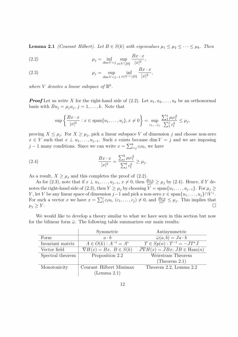
Lemma 2.1 (Courant–Hilbert). Let B ∈ S(k) with eigenvalues µ1 ≤ µ2 ≤ · · · ≤ µk. Then

µj = infdimV=j

supx∈V \0

Bx · x|x|2

,(2.2)

µj = supdimV=j−1

infx∈V ⊥\0

Bx · x|x|2

,(2.3)

where V denotes a linear subspace of Rk.

Proof Let us write X for the right-hand side of (2.2). Let u1, u2, . . . , uk be an orthonormalbasis with Buj = µjuj, j = 1, . . . , k. Note that

sup

Bx · x|x|2

: x ∈ spanu1, . . . , uj, x 6= 0

= sup

c1,...,cj

∑j1 µlc

2l∑j

1 c2l

≤ µj,

proving X ≤ µj. For X ≥ µj, pick a linear subspace V of dimension j and choose non-zerox ∈ V such that x ⊥ u1, . . . , uj−1. Such x exists because dimV = j and we are imposing

j − 1 many conditions. Since we can write x =∑k

l=j clul, we have

(2.4)Bx · x|x|2

=

∑kj µlc

2l∑k

j c2l

≥ µj.

As a result, X ≥ µj and this completes the proof of (2.2).As for (2.3), note that if x ⊥ u1, . . . , uj−1, x 6= 0, then Bx·x

|x|2 ≥ µj by (2.4). Hence, if Y de-

notes the right-hand side of (2.3), then Y ≥ µj by choosing V = spanu1, . . . , uj−1. For µj ≥Y , let V be any linear space of dimension j−1 and pick a non-zero x ∈ spanu1, . . . , uj∩V ⊥.For such a vector x we have x =

∑j1 clul, (c1, . . . , cj) 6= 0, and Bx·x

|x|2 ≤ µj. This implies thatµj ≥ Y .

We would like to develop a theory similar to what we have seen in this section but nowfor the bilinear form ω. The following table summarizes our main results:

Symmetric AntisymmetricForm a · b ω(a, b) = Ja · bInvariant matrix A ∈ O(k) : A−1 = A∗ T ∈ Sp(n) : T−1 = −JT ∗JVector field ∇H(x) = Bx, B ∈ S(k) J∇H(x) = JBx; JB ∈ Ham(n)Spectral theorem Proposition 2.2 Weirstrass Theorem

(Theorem 2.1)Monotonicity Courant–Hilbert Minimax Theorem 2.2, Lemma 2.2

(Lemma 2.1)

12

We say a matrix T is symplectic if ω(Ta, Tb) = ω(a, b). Equivalently T ∗JT = J orT−1 = −JT ∗J . The set of 2n × 2n symplectic matrices is denoted by Sp(n). We say amatrix C is Hamiltonian if C = JB for a symmetric matrix B. The space of 2n × 2nHamiltonian matrices is denoted by Ham(n). We have

C ∈ Ham(n)⇔ JC + C∗J = 0⇔ C∗ = JCJ.

We note that if H(x) = 12Bx · x with B ∈ S(2n), then J∇H(x) = JBx with JB ∈ Ham(n).

We are now ready to state Weirstrass Theorem which allows us to diagonalize a Hamil-tonian matrix using a symplectic change of variable.

Theorem 2.1 Let B be a positive matrix. Then the matrix C = JB has purely imaginaryeigenvalues of the form ±iλ1, . . . ,±iλn with λ1 ≥ · · · ≥ λn ≥ 0. Moreover there existsT ∈ Sp(n) such that the quadratic Hamiltonian function H(x) = 1

2Bx · x can be represented

as

H T (x) =n∑j=1

λj2

(q2j + p2

j),

where x = (q1, p1, . . . , qn, pn).

Proof Step 1. Let µ + iλ be an eigenvalue of C associated with the (non-zero) eigenvectora+ ib. As a result,

Ca = µa− λb, Cb = λa+ µb or Ba = λJb− µJa, Bb = −λJa− µJb.

HenceBa · b = µω(b, a), Bb · a = −µω(b, a), Ba · a = Bb · b = λω(b, a).

From this, B = B∗, µ + iλ 6= 0, and a + ib 6= 0, we deduce that µ = 0, ω(b, a) 6= 0, andBa · b = 0. As a result, for every nonzero eigenvalue iλ, we can find an eigenvector a + ib,such that

Ba · a = Bb · b = λ, Ba · b = 0,(2.5)

Ca = −λb, Cb = λa.

Step 2. If λ1 = 0, then all eigenvalues are 0 and there is nothing to prove. If λ1 6= 0, we useStep 1 and (2.5) find a1 and b1 such that

Ba1 · a1 = Bb1 · b1 = λ, Ba1 · b1 = 0, Ca = −λb, Cb = λa.

13

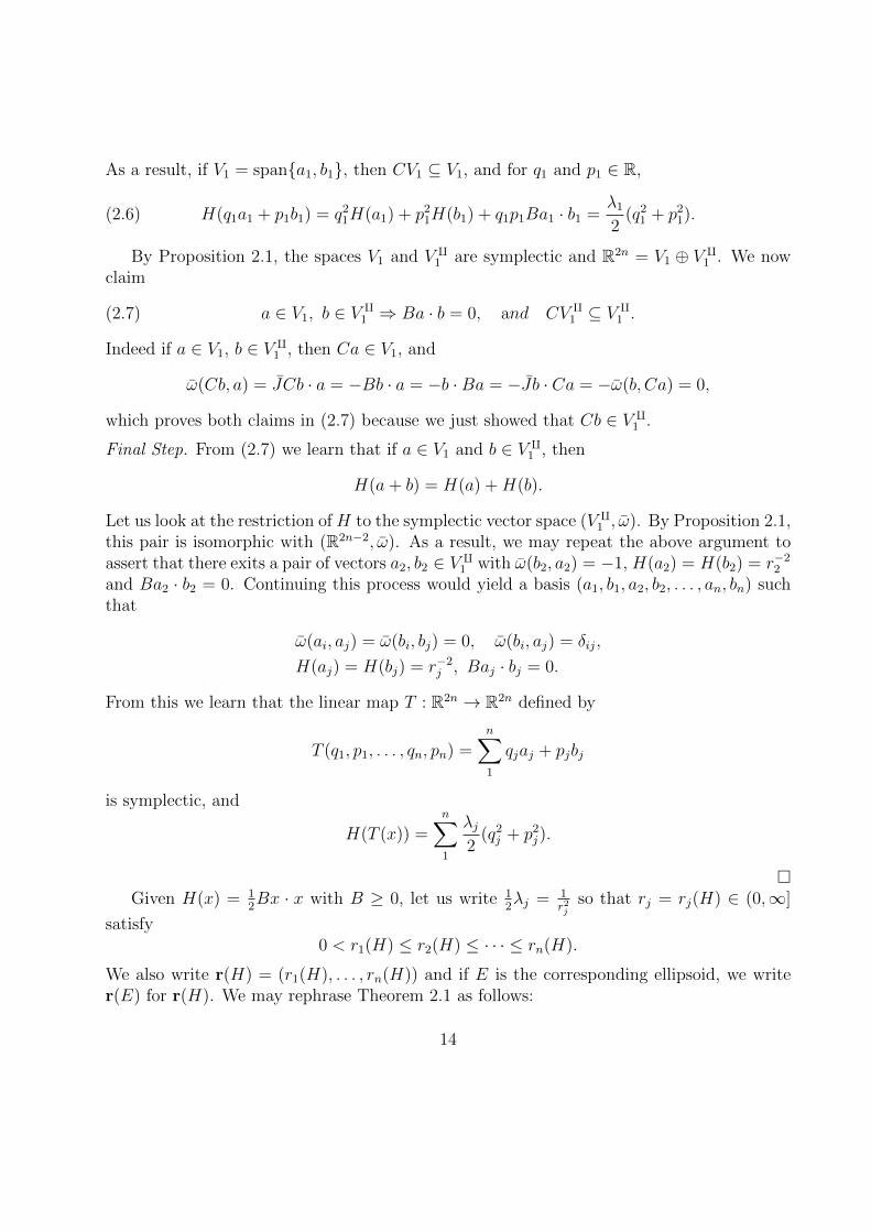
As a result, if V1 = spana1, b1, then CV1 ⊆ V1, and for q1 and p1 ∈ R,

(2.6) H(q1a1 + p1b1) = q21H(a1) + p2

1H(b1) + q1p1Ba1 · b1 =λ1

2(q2

1 + p21).

By Proposition 2.1, the spaces V1 and V q1 are symplectic and R2n = V1 ⊕ V q1 . We nowclaim

(2.7) a ∈ V1, b ∈ V q1 ⇒ Ba · b = 0, and CV q1 ⊆ V q1 .

Indeed if a ∈ V1, b ∈ V q1 , then Ca ∈ V1, and

ω(Cb, a) = JCb · a = −Bb · a = −b ·Ba = −Jb · Ca = −ω(b, Ca) = 0,

which proves both claims in (2.7) because we just showed that Cb ∈ V q1 .

Final Step. From (2.7) we learn that if a ∈ V1 and b ∈ V q1 , then

H(a+ b) = H(a) +H(b).

Let us look at the restriction of H to the symplectic vector space (V q1 , ω). By Proposition 2.1,this pair is isomorphic with (R2n−2, ω). As a result, we may repeat the above argument toassert that there exits a pair of vectors a2, b2 ∈ V q1 with ω(b2, a2) = −1, H(a2) = H(b2) = r−2

2

and Ba2 · b2 = 0. Continuing this process would yield a basis (a1, b1, a2, b2, . . . , an, bn) suchthat

ω(ai, aj) = ω(bi, bj) = 0, ω(bi, aj) = δij,

H(aj) = H(bj) = r−2j , Baj · bj = 0.

From this we learn that the linear map T : R2n → R2n defined by

T (q1, p1, . . . , qn, pn) =n∑1

qjaj + pjbj

is symplectic, and

H(T (x)) =n∑1

λj2

(q2j + p2

j).

Given H(x) = 1

2Bx · x with B ≥ 0, let us write 1

2λj = 1

r2j

so that rj = rj(H) ∈ (0,∞]

satisfy0 < r1(H) ≤ r2(H) ≤ · · · ≤ rn(H).

We also write r(H) = (r1(H), . . . , rn(H)) and if E is the corresponding ellipsoid, we writer(E) for r(H). We may rephrase Theorem 2.1 as follows:

14

Corollary 2.2 (i) If H1 and H2 are two positive definite quadratic forms, then r(H1) =r(H2) if and only if H2 = H1 T for some T ∈ Sp(n).

(ii) Let E1 and E2 be two ellipsoid. Then T (E2) = E1 for T ∈ Sp(n) if and only ifr(E1) = r(E2).

Example 2.1 Let n = 1 and H(q1, p1) =q21

R21

+p2

1

R22

so that R(H) = (R1, R2). Here H(x) =12Bx · x with

B =

[2R2

10

0 2R2

2

].

We have

C =

[0 1−1 0

]B =

[0 2

R22

− 2R2

10

].

The matrix C has eigenvalues ±i 2R1R2

. Hence r(H) = (r1(H)) with r1(H) =√R1R2 and

there exists T ∈ Sp(n) such that H T (q1, p1) =q21+p2

1

R1R2.

As our next corollary to Theorem 2.1, we solve (2.1) with the aid of a symplectic changeof coordinates:

Corollary 2.3 Let H, T and (λ1, . . . , λn) be as in Theorem 2.1. Let x(t) be a solution of(2.1) and define y(t) = T−1x(t). Then y = JB0y, where B0 is a diagonal matrix that hasthe entries

λ1, . . . , λn, λ1, . . . , λn,

on its main diagonal.

Proof From (2.1), we learn that T y = JBTy. Also, by Theorem 2.1 we know that (BTx) ·(Tx) = B0x · x, which means that T ∗BT = B0. As a result

y = T−1JBTy = −JT ∗J JBTy = JT ∗BT = JB0.

Remark 2.1 If we write φt(y) for the flow of y = JB0y and use the complex notationy = (z1, . . . , zn) with zj = qj + ipj, then

φt(z1, . . . , zn) = (e−iλ1tz1, . . . , e−iλntzn).

In particular, for each zj 6= 0, λj 6= 0, if we set zj for the complex vector that has zj for thej-coordinate and 0 for the other coordinates, then the orbit (φt(zj) : t ∈ R) is periodic ofperiod 2π/λj = πr2

j . We now turn to the question of monotonicity.

15

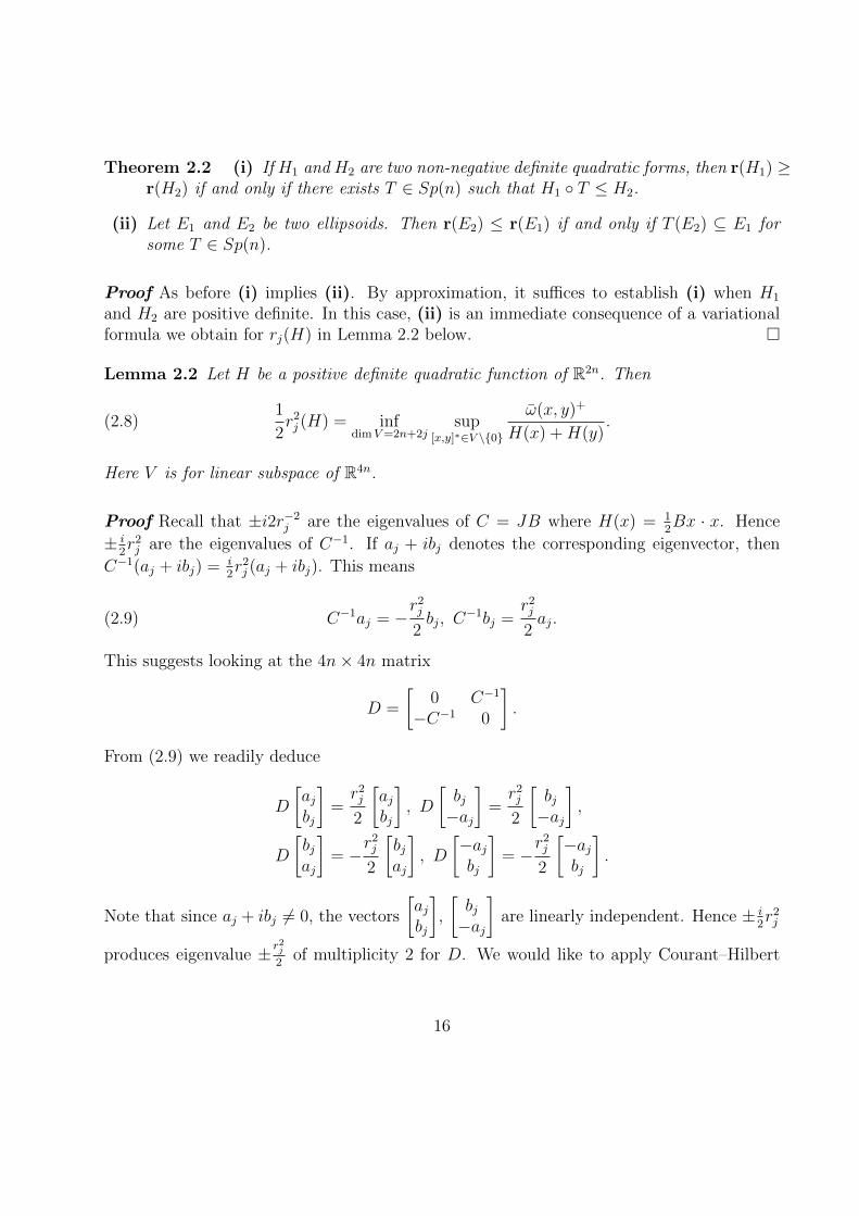
Theorem 2.2 (i) If H1 and H2 are two non-negative definite quadratic forms, then r(H1) ≥r(H2) if and only if there exists T ∈ Sp(n) such that H1 T ≤ H2.

(ii) Let E1 and E2 be two ellipsoids. Then r(E2) ≤ r(E1) if and only if T (E2) ⊆ E1 forsome T ∈ Sp(n).

Proof As before (i) implies (ii). By approximation, it suffices to establish (i) when H1

and H2 are positive definite. In this case, (ii) is an immediate consequence of a variationalformula we obtain for rj(H) in Lemma 2.2 below.

Lemma 2.2 Let H be a positive definite quadratic function of R2n. Then

(2.8)1

2r2j (H) = inf

dimV=2n+2jsup

[x,y]∗∈V \0

ω(x, y)+

H(x) +H(y).

Here V is for linear subspace of R4n.

Proof Recall that ±i2r−2j are the eigenvalues of C = JB where H(x) = 1

2Bx · x. Hence

± i2r2j are the eigenvalues of C−1. If aj + ibj denotes the corresponding eigenvector, then

C−1(aj + ibj) = i2r2j (aj + ibj). This means

(2.9) C−1aj = −r2j

2bj, C

−1bj =r2j

2aj.

This suggests looking at the 4n× 4n matrix

D =

[0 C−1

−C−1 0

].

From (2.9) we readily deduce

D

[ajbj

]=r2j

2

[ajbj

], D

[bj−aj

]=r2j

2

[bj−aj

],

D

[bjaj

]= −

r2j

2

[bjaj

], D

[−ajbj

]= −

r2j

2

[−ajbj

].

Note that since aj + ibj 6= 0, the vectors

[ajbj

],

[bj−aj

]are linearly independent. Hence ± i

2r2j

produces eigenvalue ± r2j

2of multiplicity 2 for D. We would like to apply Courant–Hilbert

16

minimax principle to D, except that D is not symmetric with respect to the dot product ofR4n. However if we define an inner product

〈[x, y]∗, [x′, y′]∗〉 = Bx · x′ +By · y′,

with corresponding norm‖[x, y]∗‖ = 2H(x) + 2H(y),

then D is 〈·, ·〉-symmetric. Indeed,⟨D

[xy

],

[x′

y′

]⟩=

⟨[C−1y−C−1x

],

[x′

y′

]⟩= BC−1y · x′ −BC−1x · y′

= Jx′ · y + Jx · y′,

which is symmetric. Moreover, ⟨D

[xy

],

[xy

]⟩= 2ω(x, y).

We are now in a position to apply Lemma 2.1 to obtain (2.8) with ω instead of ω+ in thenumerator. (Note that 1

2r2j (H) is the 2n+2j-th eigenvalue of D.) Finally we need to replace

o with ω+. This is plausible because the left-hand side is positive.

An immediate consequence of Theorem 2.2 is a linear version of Gromov’s non-squeezingtheorem. More precisely, if we define

BR = x : |x| ≤ R, ZR = x : q21 + p2

1 ≤ R2,

then r(BR) = (R,R, . . . , R) and r(ZR) = (R,∞,∞, . . . ,∞). By Theorem 2.2(ii) if for someT ∈ Sp(n), we have T (Br) ⊆ ZR, then r ≤ R. We now slightly improve this and give adirect proof of it.

Proposition 2.4 Suppose that for some T ∈ Sp(n) and z0 ∈ R2n, T (Br) ⊆ z0 + ZR. Thenr ≤ R.

Proof Write z0 = (q01, . . . , q

0n, p

01, . . . , p

0n) and let (s1, . . . , sn, t1, . . . , tn) denote the rows of T .

By assumption(x · s1 − q0

1)2 + (x · t1 − p01)2 ≤ R2

for x satisfying |x| ≤ r. Hence

(2.10) (x · s1)2 + (x · t1)2 − 2x · (q01s1 + p0

1t1) ≤ R2.

17

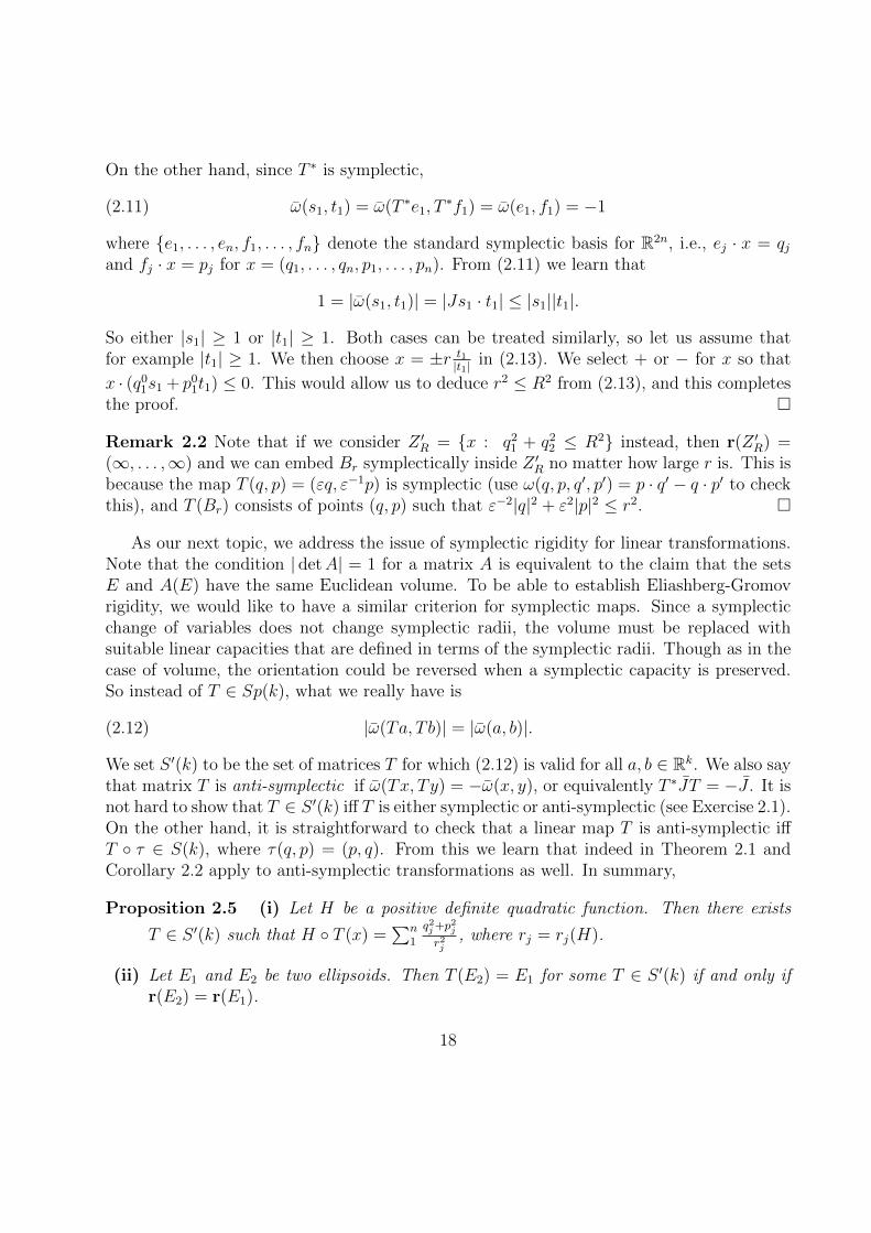
On the other hand, since T ∗ is symplectic,

(2.11) ω(s1, t1) = ω(T ∗e1, T∗f1) = ω(e1, f1) = −1

where e1, . . . , en, f1, . . . , fn denote the standard symplectic basis for R2n, i.e., ej · x = qjand fj · x = pj for x = (q1, . . . , qn, p1, . . . , pn). From (2.11) we learn that

1 = |ω(s1, t1)| = |Js1 · t1| ≤ |s1||t1|.

So either |s1| ≥ 1 or |t1| ≥ 1. Both cases can be treated similarly, so let us assume thatfor example |t1| ≥ 1. We then choose x = ±r t1

|t1| in (2.13). We select + or − for x so that

x · (q01s1 + p0

1t1) ≤ 0. This would allow us to deduce r2 ≤ R2 from (2.13), and this completesthe proof.

Remark 2.2 Note that if we consider Z ′R = x : q21 + q2

2 ≤ R2 instead, then r(Z ′R) =(∞, . . . ,∞) and we can embed Br symplectically inside Z ′R no matter how large r is. This isbecause the map T (q, p) = (εq, ε−1p) is symplectic (use ω(q, p, q′, p′) = p · q′ − q · p′ to checkthis), and T (Br) consists of points (q, p) such that ε−2|q|2 + ε2|p|2 ≤ r2.

As our next topic, we address the issue of symplectic rigidity for linear transformations.Note that the condition | detA| = 1 for a matrix A is equivalent to the claim that the setsE and A(E) have the same Euclidean volume. To be able to establish Eliashberg-Gromovrigidity, we would like to have a similar criterion for symplectic maps. Since a symplecticchange of variables does not change symplectic radii, the volume must be replaced withsuitable linear capacities that are defined in terms of the symplectic radii. Though as in thecase of volume, the orientation could be reversed when a symplectic capacity is preserved.So instead of T ∈ Sp(k), what we really have is

(2.12) |ω(Ta, Tb)| = |ω(a, b)|.

We set S ′(k) to be the set of matrices T for which (2.12) is valid for all a, b ∈ Rk. We also saythat matrix T is anti-symplectic if ω(Tx, Ty) = −ω(x, y), or equivalently T ∗JT = −J . It isnot hard to show that T ∈ S ′(k) iff T is either symplectic or anti-symplectic (see Exercise 2.1).On the other hand, it is straightforward to check that a linear map T is anti-symplectic iffT τ ∈ S(k), where τ(q, p) = (p, q). From this we learn that indeed in Theorem 2.1 andCorollary 2.2 apply to anti-symplectic transformations as well. In summary,

Proposition 2.5 (i) Let H be a positive definite quadratic function. Then there exists

T ∈ S ′(k) such that H T (x) =∑n

1

q2j+p2

j

r2j

, where rj = rj(H).

(ii) Let E1 and E2 be two ellipsoids. Then T (E2) = E1 for some T ∈ S ′(k) if and only ifr(E2) = r(E1).

18

We are now ready for a converse to Proposition 2.5, which will be used for the proof ofEliashberg’s theorem in Section 6.

Theorem 2.3 Let T be an invertible 2n× 2n matrix. Then T ∈ S ′(k) iff r1(E) = r1(T (E))for every ellipsoid E.

Proof Given a pair of vectors (a, b) with ω(a, b) 6= 0, let us define

Z(a, b) = x : (x · a)2 + (x · b)2 ≤ 1,

which is a cylinder. We claim that in fact Z(a, b) is a (degenerate) ellipsoid with

(2.13) r1(Z(a, b)) = |ω(a, b)|−1/2, rj(Z(a, b)) =∞, for j ≥ 2.

Once we establish this, we are done: If r1(Z(a, b)) = r1(T (Z(a, b)) for every a and b withω(a, b) 6= 0, then using Z(a, b) = T

(Z(T ∗a, T ∗b)

), we deduce

|ω(a, b)| = |ω(T ∗a, T ∗b)|,

whenever ω(a, b), ω(T ∗a, T ∗b) 6= 0. As a result

A := (a, b) : |ω(a, b)| 6= |ω(T ∗a, T ∗b)| ⊆ A′ := (a, b) : ω(a, b)ω(T ∗a, T ∗b) = 0.

Since the set A is open and the set A′ is the union of two linear sets of codimension 1, wemust have A = ∅, which in turn implies that T ∗ ∈ S ′(k). From this, we can readily showthat T ∈ S ′(k).

It remains to verify (2.13). First observe that if r = |ω(a, b)|−1/2 and (a1, b1) = r(a, b),then |ω(a1, b1)| = 1, and

Z(a, b) =x : H(x) :=

[(x · a′)2 + (x · b′)2

]/r2 ≤ 1

.

Without loss of generality, let us assume that in fact ω(a1, b1) = −1. We then build a(symplectic) basis a1, . . . , an, b1, . . . , bn such that

ω(bj, ai) = δi,j, ω(ai, aj) = ω(bi, bj) = 0,

for all i and j. Let us write e1, . . . , en, f1, . . . , fn for the standard basis, in other words,ei and fi satisfy ei · x = qi and fi · x = pi. We then choose a map T so that T ∗ai = ei andT ∗bi = fi. We have

H T (x) =[(T x · a1)2 + (T x · b1)2

]/r2 =

[(x · e1)2 + (x · f1)2

]/r2 = (q2

1 + p21)/r2.

From this we deduce (2.13) by definition.

19

As we observed in Remark 2.1, sometimes it is beneficiary to identify R2n with Cn anduse complex number. More precisely, we may write zj = qj + ipj, so that if a = (z1, . . . , zn)and b = (z′1, . . . , z

′n) are in Cn, then Ja = (−iz1, . . . ,−izn), and

a · b = Ren∑j=1

zj z′j, ω(a, b) = Im

n∑j=1

zj z′j.

More generally, given a symplectic vector space (V, ω), we may try to express ω as

(2.14) ω(a, b) = g(Ja, b),

where g is an inner product on V and J : V → V is a linear map satisfying J2 = −I. When(2.14) is true, we say that the pair (g, J) is compatible with ω. Let us write I(ω) for thespace of compatible pairs (g, J). We also define

G(ω) := g : (g, J) ∈ I(ω), for some J .

Note that if (g, J) ∈ I(ω), then

g(Ja, Jb) = ω(a, Jb) = −ω(Jb, a) = g(b, a) = g(a, b),

which means that J∗J = I, where J∗ is the g-adjoint or transpose of J . From this and J2 =−I, we learn that for every (g, J) ∈ I(ω), we have J∗ = −J . Define T ∗g(a, b) = g(Ta, Tb)and T ∗ω(a, b) = ω(Ta, Tb).

Proposition 2.6 Let T : V → V be an invertible linear map. Then T ∗ω = ω′ iff T ∗(G(ω)) =G(T ∗ω

).

Proof Set T (J) = T−1JT . If (g, J) ∈ I(ω), then

(T ∗ω)(a, b) = ω(Ta, Tb) = g(JTa, T b) = ω(T T (J)a, T b) = (T ∗ω)(T (J)a, b).

From this we deduce that if (g, J) ∈ I(ω), then (T ∗g, T (J)) ∈ I(T ∗ω). As a result,T ∗(G(ω)) ⊆ G(T ∗ω). Similarly, (T−1)∗G(T ∗ω) ⊆ G(ω). Hence T ∗(G(ω)) = G(T ∗ω).

Example 2.2 Identifying a metric g(a, b) = Ga · b with the matrix G > 0, one can readilyshow

(2.15) G(ω) = G : G > 0, G ∈ S(2n).

Indeed if g(a, b) = Ga · b and (g, J) ∈ I(ω), then J = GJ so that G = −JJ. This implies

GJG = JJJ JJ = J ,

20

which means that G is symplectic. Conversely, if G > 0 and G ∈ S(2n), then set J = G−1Jand observe that since G−1 is also symplectic, then J2 = G−1JG−1J = J J = −I.

When g ∈ G(ω), we know how to calculate the area of the parallelogram associated withtwo vectors a and b, namely

Ag(a, b) =(‖a‖2

g‖b‖2g − g(a, b)2

) 12 ,

where ‖a‖g = g(a, a)1/2. Of course ω(a, b) offers the symplectic area of the same parallelo-gram. In the next proposition, we compare these two areas.

Proposition 2.7 For every g ∈ G(ω), we have

(2.16) ω(a, b) ≤ Ag(a, b) ≤1

2

(‖a‖2

g + ‖b‖2g

).

Moreover we have equality iff b = Ja.

Proof The second inequality is obvious and the first inequality is also obvious when g(a, b) =0, because

ω(a, b)2 = g(Ja, b)2 ≤ g(Ja, Jb)g(b, b) = ‖a‖2g‖b‖2

g.

Given arbitrary a and b, with a 6= 0, set t = −g(a, b)/g(a, a) so that g(a, b′) = 0, forb′ = ta+ b. We certainly have

ω(a, b)2 = ω(a, b′)2 ≤ g(Ja, Ja)g(b′, b′) = g(a, a)g(b′, b′) = g(a, a)g(b′, b)

= g(a, a)g(b, b) + tg(a, a)g(a, b) = Ag(a, b),

with equality iff Ja = θb′ for some θ ≥ 0. However, if we require 2ω(a, b)2 = ‖a‖2g + ‖b‖2

g,then g(a, b) = 0, g(a, a) = g(b, b), and ω(a, b)2 = g(a, a)2. As a result,

‖Ja− b‖2g = ‖a‖2

g + ‖b‖2g − 2g(Ja, b) = 2‖a‖2

g − 2ω(a, b) = 0,

as desired.

Exercise 2.1

(i) Let V be a vector space with dimV = 2n. Then a 2-form ω : V × V → R is non-degenerate if and only if ωn = ω ∧ · · · ∧ ω︸ ︷︷ ︸

n times

6= 0.

(ii) Use part (i) to deduce that if T ∈ Sp(n), then detT = 1.

(iii) Recall that an invertible matrix T can be written as T = PO with P > 0 symmetricand O orthogonal, and that this decomposition is unique (polar decomposition). Showthat if T ∈ Sp(n), then P and O ∈ Sp(n).

21

(iv) Show that if T ∈ Sp(n) ∩ O(2n), then T =

[X −YY X

]with X, Y two n × n matrices

such that X + iY is a unitary matrix.

(v) Let V be a vector space with dimV = 2n + 1. Assume β is an antisymmetric 2-formon V with

dimv ∈ V : β(v, a) = 0 for all a ∈ V ) = 1.

Then there exists a basis e1, . . . , en, f1, . . . , fn, a such that β(ei, ej) = β(fi, fj) = 0,β(fj, ei) = δij, and β(a, fj) = β(a, ej) = 0.

(vi) If T ∈ Sp(n) and A ∈ Ham(n), then T−1AT ∈ Ham(n).

(vii) An invertible T maps the flows of dxdt

= Ax to the flows of dxdt

= Bx iff B = TAT−1.

(viii) If C1, C2 ∈ Ham(n) and r ∈ R, then C1+C2, [C1, C2] = C1C2−C2C1, Ct1, rC1 ∈ Ham(n).

(ix) If T1, T2 ∈ Sp(n), then T−11 , T ∗1 , T1T2 ∈ Sp(n).

(x) Show that if (2.13) is true for all a and b, then T is either symplectic or ani-symplectic.

(xi) If Z(t0, t) denotes the fundamental solution of x = JB(t)x with B : [t0,∞)→ S(2n) aC1-function, then Z(t0, t) ∈ Sp(n) for every t ≥ t0.

(xii) If etC ∈ Sp(n) for every t, then C ∈ Ham(n).

(xiii) If C ∈ Ham(n), and pC(λ) = det(λI − C), then pC(λ) = pC(−λ).

(xiv) If T ∈ Sp(n), then pT (λ−1) = λ−2npT (λ).

(xv) Let T be an invertible matrix and assume that n ≥ 2. Show that if r2(T (E)) = r2(E)for every ellipsoid E, then T ∈ S ′(2n).

22

3 Symplectic Manifolds and Darboux’s Theorem

Before discussing symplectic manifolds, let us review some useful facts about our basicexample (R2n, ω) with ω(a, b) = Ja · b. We write Sp(R2n) for the space of differentiablefunctions ϕ such that ϕ∗ω = ω. This means

ϕ∗ω(a, b) = ω(ϕ′(x)a, ϕ′(x)b) = ω(a, b),

for every a, b, x ∈ R2n. Here ϕ′(x) denotes the derivative of ϕ. A function ϕ ∈ Sp(R2n)is called symplectic. Note that ϕ ∈ Sp(R2n) iff ϕ′(x) ∈ Sp(2n) for every x. Hence for asymplectic transformation ϕ, we have

ϕ′(x)∗Jϕ′(x) = J .

Evidently ω =∑n

i=1 dpi ∧ dqi = dλ where λ =∑n

1 pidqi = p · dq. Let us define

(3.1) A(γ) =

∫γ

λ.

Clearly ϕ ∈ Sp(R2n) iff d(ϕ∗λ− λ) = 0. Hence ϕ ∈ Sp(R2n) is equivalent to saying

(3.2) A(ϕ γ) = A(γ)

for every closed curve γ. It is worth mentioning that if γ is parametrized by θ 7→ x(θ),θ ∈ [0, T ], then

(3.3) A(γ) =

∫ T

0

p · qdθ =1

2

∫ 1

0

(p · q − q · p)dθ =1

2

∫ 1

0

(Jx · x)dθ.

Given a scalar-valued (0-form) function H, we may use non-degeneracy of ω to define avector-field XH such that

ω(XH(x), a) = −dH(x)a = −∇H(x) · a,

which means that XH = J∇H. We write φt = φHt for the corresponding flow:

(3.4)

ddtφt(x) = XH(φt(x)),

φ0(x) = x.

Our interest in symplectic transformation stems from two important facts. Firstly, φt ∈Sp(R2n) if φt is a Hamiltonian flow. We have seen this in Section 1 and will be proved laterin this section for general symplectic manifolds. Secondly a symplectic change of coordinatespreserve Hamiltonian structure (see Proposition 3.1 below). More precisely, if ϕ ∈ Sp(R2n),

23

and φt is the flow of XH , then ψt = ϕ−1 φt ϕ is the flow of a Hamiltonian system. Toguess what the Hamiltonian function of ψt is, observe

d

dtψt

∣∣∣∣t=0

= (ϕ−1)′ ϕ XH ϕ = (ϕ′)−1 J∇H ϕ

= −J(ϕ′)∗ J J∇H ϕ = J(ϕ′)∗ ∇H ϕ = J∇(H ϕ).

A pair (M,ω) is called a symplectic manifold if M is an even dimensional manifold and ωis a closed non-degenerate 2-form on M . This implies that for each x ∈M , the pair (TxM,ωx)is a symplectic vector space. Also, by Exercise 2.1(i) we know that if dim(M) = 2n, thenthe form ωn is a volume form. Hence M is an orientable manifold. In fact if M is a compactsymplectic manifold without boundary, then ω is never exact. This is because if ω = dλ,then Ω := ωn = d(λ ∧ ωn−1). But by Stokes’ theorem

∫M

Ω =∫Md(λ ∧ ωn−1) = 0, which

contradicts the non-degeneracy of Ω. Note however that (R2n, ω) is an example of a non-compact symplectic manifold with ω = dλ.

Example 3.1 (i) Any orientable 2-dimensional manifold is symplectic where ω is chosen tobe any volume form.

(ii) The sphere S2n with n > 1 is not symplectic because any closed 2-form is exact, hencedegenerate.

(iii) The classical example (R2n, ω) has a natural generalization that is relavant for models inclassical mechanics: Every cotangent bundle T ∗M can be equipped with a symplectic ω = dλwhere λ is a standard 1-form that can be defined in two ways; using local charts and pull-backing λ to λ, or giving a chart-free description. We start with the former. Let us assumethat M is an n-dimensional C2 manifold and choose an atlasA of charts (U, h) of M such thatU is an open subset of M and h : U → h(U) := V ⊆ Rn is a diffeomorphism. This inducesa C1 transformation dh : TU → TV = V × Rn. We next define a natural transformationh : T ∗U → T ∗V = V × Rn. To construct h, take the standard basis e1, . . . , en of Rn

and define ej(q) = (dφ)q(ej), where φ = h−1. (We may define TqM as the equivalenceclasses of curves γ : (−δ, δ) → M with γ(0) = q, and two such curves γ1 and γ2 areequivalent if (h γ1)′(0) = (h γ2)′(0). We may then define ej(q) as the equivalent class ofγj(θ) = h−1(h(q)+θej). ) Certainly e1(q), . . . , en(q) defines a basis for TqM . We now define

a basis for T ∗q L by taking dual vectors e∗1, . . . , e∗n that are defined e∗i (q)

(∑nj=1 vj ej(q)

)= vj.

We now define h by

h

(q,

n∑j=1

pje∗j(q)

)= (h(q), (p1, . . . , pn)).

We finally define λ as the unique 1-form such that for each chart (U, h), the restriction ofλ to T ∗U is given by λ = h∗λ. For an alternative chart-free description, observe that if

24

π : T ∗Rn → Rn is the projection π(q, p) = q, then

dπ : T (T ∗Rn)→ TRn = Rn × Rn

is simply given bydπ(q,p)(α, β) = α.

Hence we may write λ(q,p)(α, β) = p · α = p · (dπ)(q,p)(α, β). Going back to M , let us alsodefine π : T ∗M → M to be the projection onto the base point, i.e., π(q, p) = q with q ∈ Mand p ∈ T ∗qM . Since the following diagram commutes

T ∗Uπ−−−→ U

h

y yhR2n −−−→

πRn

we also have that their derivatives

T (T ∗U)dπ−−−→ TU

dh

y ydhTR2n −−−→

dπR2n

commute. Hence we also have

λ(q,p)(a) = p(dπ(q,p)(a)

),

which gives the desired chart-free description of λ.

A differentiable map f : (M1, ω1)→ (M2, ω

2) between two symplectic manifolds is calledsymplectic if f ∗ω2 = ω1. This means

(3.5) ω2f(x)(df(x)a, df(x)b) = ω1

x(a, b)

for x ∈ M1 and a, b ∈ TxM1. We write Sp(M1,M2) for the space of symplectic transforma-tions. When M1 = M2 = M and ω1 = ω2 = ω, we simply write Sp(M) for Sp(M1,M2).We note that if f ∈ Sp(M1,M2), then df(x) is injective by (3.5) and non-degeneracy of ω1

x.Hence, if such f exists, then dimM1 ≤ dimM2.

Let (M,ω) be a symplectic manifold and assume that X is sufficiently nice vector fieldfor which the ODE x = X(x, t) is well defined. The flow of this vector field is denoted byφt = φXt . We wish to find conditions on X to guarantee that φ∗tω = ω. To prepare for thislet us take an arbitrary `-form α and evolve it with the flow; set α(t) = φ∗tα. We would liketo derive an evolution equation for α(t). Let’s examine some examples.

Example 3.2 Assume that (M,ω) = (R2n, ω).

25

(i) If α = f is a 0-form, then α(t) is a function u that is given by u(x, t) = f(φt(x)). Bydifferentiating u at t = 0 and using the group property of the flow (see the proof ofProposition 3.1 below), we can readily show

ut = X · ux.

(ii) If α = m(x) dx1 . . . dxk, with k = 2n, then α(t) = m(φt(x)) det(φ′t(x)) dx1 . . . dxk. Inthis case, differentiating in t yields,

ρt = ρx ·X + ρ divX = div(ρX),

because for small t, we have det(φ′t(x)) = det(I + tX ′(x) + o(t)) = 1 + tdivX + o(t).

(iii) If ω = F · dx is a 1-form, then

α(t) = φ∗tα = F (φt(x)) · φ′t(x)dx = φ′t(x)∗F (φt(x)) · dx.

Hence, if we set u(x, t) = φ′t(x)∗F (φt(x)), then

(3.6) ut(x, t) = Xx(x, t)∗u(x, t) + ux(x, t)X(x, t).

If u = (u1, . . . , uk) and X = (X1, . . . , Xk), then the i-th component of the right-handside of (3.6) equals∑

j

(Xjxiuj + uixjX

j)

=

(∑j

Xjuj

)xi

+∑j

(uixj − ujxi

)Xj.

As a result,

(3.7) ut = (X · u)x + C(u)X.

As Example 3.2(iii) indicates, a simple manipulation of the right-hand side of (3.6) leadsto the compact expression of the right-hand side of (3.7), that may be recognized as

[(X · u)x + C(u)X] · dx = d (iXα(t)) + iXdα(t).

More generally we have the following useful result of Cartan:

Proposition 3.1 (i) Let X be a vector field with flow φt and let α be a `-form. Then

(3.8)d

dtφ∗tα = LXφ∗tα = φ∗tLXα

with LX = iX d+ d iX .(ii) Let X(·, t) be a possibly time dependent vector field and denote is flow by φs,t. If φt = φ0,t,

thend

dtφ∗tα = φ∗tLX(·,t)α.

26

Proof (i) Let us define

Lβ = limh→0

1

h(φ∗hβ − β)

whenever the limit exists. Since

(φ∗t+h − φ∗t )α = φ∗t (φ∗hα− α) = φ∗h(φ

∗tα)− φ∗tα,

it suffices to show that L = LX . Let us study some properties of L. From φ∗t (α ∧ β) =φ∗tα ∧ φ∗tβ, we learn

φ∗t (α ∧ β)− α ∧ β = (φ∗tα− α) ∧ φ∗tβ + α ∧ (φ∗tβ − β).

From this we deduce

(3.9) L(α ∧ β) = α ∧ Lβ + Lα ∧ β.

From φ∗t d = d φ∗t , we deduce

(3.10) L d = d L.

We can readily show that LX satisfy (3.9) and (3.10) as well. Since locally every form canbe built from 0-th forms using the operations ∧ and d, we only need to check that L = LXon 0-forms. That is, if f : M → R, then Lf = iX df = df(X). This is trivially verifiedbecause φh(x) = x+ hX(x) + o(h).

(ii) For h > 0, we write(φ∗t+h − φ∗t )α = φ∗t (φ

∗t,t+hα− α).

A repetition of the proof of Part (i) leads to

limh→0

1

h

(φ∗t,t+hβ − β

)= LX(·,t)β.

This readily implies Part (ii).

Armed with (3.8), we can readily find necessary and sufficient conditions on a vector fieldX such that the flow of X preserves ω. In view of Proposition 3.1,(

φXt)∗ω = ω for all t ⇔ LXω = d (iXω) = 0.

This leads to two definitions:

Definition 3.1

• We call a vector field X symplectic iff iXω is exact.

27

• Given a differentiable H : M → R, we can find a unique vector field X = XH = XωH

such that(iXHω) = ω(XH , ·) = −dH.

(Note that the non-degeneracy of ω guarantees the existence XH .) The vector fieldXH is called Hamiltonian and its corresponding flow is denoted by φHt .

Example 3.2 If ωx(v1, v2) = C(x)v1 · v2 is a symplectic form in R2n, then XH = −C−1∇H.

As in the case of ω, a change of coordinates turn a Hamiltonian flow to another Hamil-tonian flow as our next Proposition demonstrates.

Proposition 3.2 Let (M,ω) be a symplectic manifold. If ϕ : N → M is a diffeomorphismand H : M → R is a smooth Hamiltonian, then Xϕ∗ω

Hϕ = (dϕ)−1XωH ϕ. In other words,

ϕ∗XωH = Xϕ∗ω

Hϕ, and

ϕ−1 φXωH

t ϕ = φϕ∗Xω

Ht = φ

Xϕ∗ωHϕ

t ,

where φXt denotes the flow of the vector field X.

Proof By Lemma 10.2 of Appendix A, ψt is the flow of ϕ∗XωH . Furthermore, for X = Xω

H

and X = (dϕ)−1X ϕ,

(ϕ∗ω)x(X(x), v) = ωϕ(x)

((dϕ)xX(x), (dϕ)xv

)= ωϕ(x) (X(ϕ(x)), (dϕ)xv)

= −(dH)ϕ(x) ((dϕ)xv) = − (ϕ∗(dH))x (v) = −d(H ϕ)x(v),

for every v. Hence X = Xϕ∗ωHϕ, as desired.

We now turn to the question of the equivalence of two symplectic manifolds or theembedding of one symplectic manifold inside another symplectic manifold. As a warm-up,let us discuss the analogous question for volume forms.

Theorem 3.1 (Moser) Let M be a connected oriented compact manifold with no boundary.Assume that α and β are two volume forms. Then there exists a diffeomorphism ϕ such thatϕ∗α = β iff

∫Mα =

∫Mβ.

Proof Evidently if for some diffeomorphism ϕ, we have ϕ∗α = β, then∫M

β =

∫M

ϕ∗α =

∫ϕ(M)

α =

∫M

α.

28

As for the converse, assume that c =∫Mα =

∫Mβ. Without loss of generality, we may

assume that c = 1, and regard α and β as two mass (or probability) distributions on M .We may interpret ϕ as a plan of transportation; a unit mass at x is transported to φ(x)so that after this transportation is performed for all points, the mass distribution changesfrom α to β. With this interpretation in mind, we may design a route for our transportationso that this change of transportation is carried out in one unit of time. Equivalently, wemay search for a (possibly time dependent) vector field X such that if φt denotes its flow,then ϕ = φ1. Note that if we set α(t) = φ∗tα, then α(0) = α and α(1) = β. This schemeof finding ϕ has a chance to work only if there exists a path of volume forms connectingα to β. So for achieving our goal, let us first such a path. We now argue that in factthe path α(t) = tβ + (1 − t)α would do the job. Since α and β are volume forms, locallyα = a dx1∧· · ·∧dxk and β = b dx1 · · ·∧ . . . dxk with a and b non-zero and continuous. Since∫Mα =

∫Mβ, the functions a and b must have the same sign. Hence tβ + (1 − t)α is never

zero, and as a result, α(t) is never degenerate. We next search for a vector field X(·, t) suchthat its flow φt satisfies φ∗tα = tβ + (1 − t)α. Differentiating both sides with respect to tyields

β − α =d

dtα(t) = LXα(t) = d(iX(·,t)α(t)).

by Proposition 3.1. But∫M

(β − α) = 0 implies that β − α = dγ for some k − 1-form γ (SeeLemma A1 of the Appendix). The existence of X(·, t) with iX(·,t)α(t) = γ follows from thenon-degeneracy of α(t).

Remark 3.1. (i) As a consequence of Theorem 3.1, if M and N are two oriented compactclosed manifolds with volume forms α and η respectively, then they there exists a diffeomor-phism φ : N →M with φ∗α = η iff M and N are diffeomorphic and

∫Mα =

∫Nη. Indeed if

ψ : M → N is a diffeomorphism, then α and β = ψ∗η are two volume forms on M for whichTheorem 3.1 applies: there exists a diffeomorphism ϕ : M → M , such that φ∗α = ψ∗η. Wethen set φ = φ ψ−1 to deduce that φ∗α = η.

(ii) If M = Tk and α = α(x) dx1 ∧ · · · ∧ dxk, β = β(x) dx1 ∧ · · · ∧ dxk, then ϕ∗α = β meansthat α(ϕ(x)) detϕ′(x) = β(x). If ϕ = ∇w for some w : Tk → R, then α(∇w) det(D2w) = β.This is the celebrated Monge–Ampere’s equation. However the function ϕ in Moser’s proofis not a gradient. In fact the vector field X in the proof of Theorem 3.1 can be constructedby the following recipe: First find a vector field Y such that div Y = β − α, so that ifγ =

∑k1(−1)j−1Y jdx1 ∧ · · · ∧ dxj ∧ · · · ∧ dxk, then dγ = β − α. Such a vector field Y exists

because∫

(β − α)dx = 0. We then set

X(x, t) = − Y (x)

tβ(x) + (1− t)α(x).

In fact for the existence of Y , we may try a gradient Y = ∇u so that the scalar-valuedfunction u satisfies ∆u = β− α. Again this equation has a solution because

∫(β− α)dx = 0.

29

(iii) There has been new developments for Moser’s theorem. In fact the transformation ϕin Theorem 3.1 is by no means unique. However, one may wonder whether or not a “nice”ϕ exists. More precisely, let (M, g) be a Riemannian manifold. Assume that M is compact,connected with no boundary. Using g we can talk about a Riemannian distance. Moreprecisely, let d(x, y) be the length of the geodesic distance between two points x and y.We have a natural volume form Ω that is expressed by (det[gij])

1/2dx1 ∧ · · · ∧ dxk in localcoordinates. Consider two forms α = aΩ and β = bΩ with a, b > 0 and

∫Mα =

∫Mβ = 1.

SetS(α, β) = f : M →M with ϕ∗α = β.

By Moser’s theorem, this set is non-empty. Monge’s problem searches for a function f ∈S(α, β) which minimizes the cost function

I(f) =

∫M

c(x, f(x))β,

with c(x, y) a suitable function of M × M . If we choose c(x, y) = 12(d(x, y))2, then the

minimizer ϕ is of the form ϕ = ∇w for a convex function w. This was shown by Brenier(1987, 1991) in the Euclidean case and by McCann in (2001) in the case of a Riemannianmanifold. Brenier observed that such a minimizer can be used to find a non-linear polardecomposition. To explain this, let F : U → Rk be an invertible integrable function withα = (F−1)∗β where β = dx1 ∧ · · · ∧ dxk and α is a volume form. According to Brenier’stheorem, there exists a convex function ψ such that (∇ψ)∗α = β. If we write ρ = (∇ψ)−1F ,then ρ∗β = F ∗(∇ψ)−1∗β = F ∗α = β. As a consequence, any function F can be decomposedas F = ∇ψρ with ψ convex and ρ volume preserving. It turns out that polar decompositionimplies the Hodge decomposition. To see this assume that F ε(x) = x + εf(x) with ε small.We then expect to have ψε(x) = 1

2|x|2 + εϕ(x) + o(ε) and ρε(x) = x+ εm(x) + o(ε). Hence

x+ εf(x) = x+ ε∇ϕ(x+ εm(x)) + εm(x) + o(ε)

= x+ ε(∇ϕ(x) +m(x)) + o(ε).(3.11)

On the other hand, since ρε is volume preserving,

1 = det(id+ εm′) = 1 + ε div(m) + o(ε).

From this and (3.11) we learn

f(x) = ∇ϕ(x) +m(x) with div m = 0.

(iv) Theorem 3.1 can be used to show that the total volume is the only invariant of volumepreserving diffeomorphisms. More precisely, if

V(M) = α : α is a volume form on M

30

with M compact and closed, andc : V(M)→ R

is a function such that c(α) = c(β) whenever ϕ∗α = β for some diffeomorphism ϕ, then cmust be a function of

∫Mα.

Given a manifold M with two symplectic forms α and β, we may wonder whether ornot for some diffeomorphism ϕ, we have ϕ∗α = β. By Theorem 3.1, this would be thecase if dim M = 2 and

∫Mα =

∫Mβ. However, when dim M = 2n ≥ 4, we may have

non-isomorphic symplectic forms α and β with∫Mαn =

∫Mβn. To see how the proof of

Theorem 3.1 breaks down, we note that we may fail to find a path of symplectic forms α(t)that connects α to β. Even if such a path exists, the equation LXα(t) = d iXα(t) = dα(t)/dtrequires that dα(t)/dt to be exact for t ∈ [0, 1]. Though both of these issues can be handledlocally as the next theorem demonstrate.

Theorem 3.2 (Darboux) Let (M,ω) be a symplectic manifold of dimension 2n and takex0 ∈M . Then there exists an open set U ⊆ R2n with 0 ∈ U and a diffeomorphism ϕ : U →Msuch that ϕ(0) = x0 and ϕ∗ω = ω.

Proof Since M is locally diffeomorphic to an open subset of R2n, we may assume thatM = U0 ⊆ R2n and x0 = 0 ∈ U . In view of Proposition 2.1, we may also assume that ω0 = ω.Our goal is finding an open set U ⊆ U0 with 0 ∈ U , and a diffeomorphism ϕ : U → U withϕ(0) = 0 and ϕ∗ω = ω = ω0. Indeed if ωx(v1, v2) = C(x)v1 · v2 and ω(t) = ω + t(ω − ω), fort ∈ [0, 1], then ω(t)x(v1, v2) = C(x, t)v1 · v2, with C(x, t) = J + t(C(x) − J) and C(0) = J .Clearly, we can find an open neighborhood U = Br(0) of 0 such that for x ∈ U we have that‖C(x)−J‖ < ‖J‖ = 1, which in turn guarantees that C(x, t) is invertible for (x, t) ∈ U×[0, 1].This means that in U , the form ω(t) is symplectic for all t ∈ [0, 1]. We then search for atime-dependent vector field X(·, t) such that its flow φt satisfies

φ∗tω = ω(t) for t ∈ [0, 1].

From differentiating both sides with respect to t and using Proposition 3.1, we learn

(3.12) ω − ω = LX(·,t)ω(t) = d iX(·,t)ω(t).

In the ball U = Br(0), we can express ω − ω = dα for a 1-form α such that α0 = 0. Hence(3.12) would follow if we can find a time-dependent vector field X such that iX(·,t)ω(t) = α.By nondegeneracy of ω(t), such a vector field X exists with X(0, t) = 0 for every t ∈ [0, 1].We are done.

Remark 3.2 If we write ω = u · dx and ω = u · dx near the origin, then X constructed inthe proof has the form

X(x, t) = C(tu(x) + (1− t)u(x)

)−1(u(x)− u(x)) = C(x, t)−1(u(x)− u(x)).

31

As an immediate consequence of Darboux’s theorem we learn that any symplectic mani-fold M of dimension 2n has a an atlas consisting of pairs (Uj, hj with hj : Uj → R2n, suchthat

hi h−1j : hj(Ui ∩ Uj)→ hi(Ui ∩ Uj)

is symplectic for every i and j. The family (Uj, hj) is an example of a symplectic atlasthat always exists by Darboux’s theorem.

Exercise 3.1 (i) Show that LX = d iX + iX d satisfy

LX d = d LX , LX(α ∧ β) = (LXα) ∧ β + α ∧ (LXβ) .

(ii) Let (M,ω) be a 2n-dimensional symplectic manifold. Assume that M is compact withno boundary. Then for every j ∈ 1, . . . , n, there exists a closed 2j-form which is not exact.

(iii) Let (M1, ω1) and (M2, ω

2) be two symplectic manifolds. Define (M1×M2, ω1×ω2) with

(ω1 × ω2)(x,y)((a1, a2), (b1, b2)) = ω1x(a1, b1) + ω2

y(a2, b2).

Show that (M1 ×M2, ω1 × ω2) is symplectic.

(iv) Let (M,ω) be a symplectic manifold. Show that if ϕ∗ω = fω for some diffeomorphismϕ : M →M , and C1 scalar function f , then either dim M = 2 or f is a constant function.

(v) Use polar coordinates in R2n to write qi = ri cos θi, pi = ri sin θi, and let ei (respectivelyfi) denote the vector for which the qi-th coordinate (respectively pi-th coordinate) is 1 andany other coordinate is 0. Set

ei(θi) = (cos θi)ei + (sin θi)fi, fi(θi) = −(sin θi)ei + (cos θi)fi.

Given a vector field u, we may write

u =n∑i=1

(aiei(θi) + bifi(θi)

).

The form α = u · dx can be written as

α =n∑i=1

(aidri + rib

idθi)

=:n∑i=1

(aidri +Bidθi

).

Assume that all ais and bis depend on r = (r1, . . . , rn) only. What are the the necessary andsufficient conditions on a and B in order for ω = dα to be symplectic.

32

(vi) Let U1 and U2 ⊂ Br be two planar open sets with smooth boundaries that are diffeomor-phic to a disc. Show that if area(U1) = U2, then there is an area preserving diffeomorphismψ : R2 → R2 such that ψ(U1) = U2 and ψ(x) = x for x /∈ Br. Here Br = x : |x| < r.Hint: Construct ψ from three diffeomrphisms ψ1, ψ2 and ψ3 with the following properties:

• ψ1 : R2 → R2 with ψ1(x) = x, for x /∈ Br, ψ1(U1) = U2, and ψ1 is area-preserving on asmall neigberhood of ∂U1.

• ψ2 : U1 → U2 is area preserving and ψ2(x) = ψ1(x) for x near ∂U1.

• ψ3 : Br \ U1 → Br \ U2 is area-preserving and ψ3(x) = ψ1(x) for x near ∂U1 ∪ ∂Br.

33

4 Contact Manifolds and Weinstein Conjecture

In this section we will give two motivations for studying contact manifolds. As our firstmotivation we observe that we can construct exotic symplectic forms on R4 from certaincontact forms in R3. Our second motivation is the Weinstein’s conjecture that predicts everycompact nonsingular contact level set of a Hamiltonian function carries at least one periodicorbit of the corresponding Hamiltonian vector field.

We first give a simple recipe for constructing a symplectic form on M = M × R fromcertain 1-forms on a manifold M : Given a 1-form α on M , define α(x,s)(v, τ) = esαx(v) forevery x ∈ M , v ∈ TxM , and s, τ ∈ R. There is nothing special about es and our approachis applicable if we replace es with a strictly increasing or decreasing C1 function of s. Thequestion is whether or not ω = dα is symplectic.

Proposition 4.1 Let M be any manifold of odd dimension and α any 1-form on M . Thenthe form dα is symplectic iff `x(α) ∩ ξx(α) = 0 for every x ∈M , where

`x = `x(α) = v ∈ TxM : dαx(v, w) = 0 for every w ∈ TxM ,ξx = ξx(α) = kerαx = v ∈ TxM : αx(v) = 0 .

Proof We certainly have dα = es(dα− α ∧ ds

). As a result,

(dα)(x,s)

((v, τ), (w, τ ′)

)= es

((dα)x(v, w)− αx(v)τ ′ + αx(w)τ

).

From this we can readily show that if v ∈ `x ∩ ξx, then

(dα)(x,s)

((v, 0), (w, τ ′)

)= 0,

for every (w, τ ′) ∈ TxM × R.Conversely, suppose that `x(α) ∩ ξx(α) = 0, and that for some (v, τ) ∈ TxM × R, we

have

(4.1) (dα)x(v, w)− αx(v)τ ′ + αx(w)τ = 0,

for every (w, τ ′) ∈ TxM × R. We wish to show that (v, τ) = 0. To see this, first vary τ ′ in(4.1), to deduce that αx(v) = 0, or v ∈ ξx. Hence we now have

(4.2) (dα)x(v, w) + αx(w)τ = 0,

for every w ∈ TxM . If τ = 0, then (4.2) means that v ∈ `x. As a result, v ∈ `x ∩ ξx = 0and we are done. On the other hand, if τ 6= 0, choose any non-zero w ∈ `x in (4.2) to deducethat αx(w) = 0, or w ∈ ξx, which contradicts our assumption `x∩ ξx = 0. (Note that sincethe dimension of M is odd, `x 6= 0.) This completes the proof.

34

Note that since dimM = 2n − 1 is odd, the dimension of `x is at least 1. Hence thecondition `x ∩ ξx = 0 implies that dim `x = 1 and dim ξx = 2n− 2. Equivalently,

(4.3) TxM = `x ⊕ ξx,

for every x ∈M .

Definition 4.1 The pair (M,α) of a manifold M and 1-form α is called a contact manifoldif `x(α) ∩ ξx(α) = 0 for every x ∈ M . The Reeb vector field R = Rα is the unique R ∈ `xsuch that α(R) = 1. The R-projection onto ξ is denoted by π = πα; πx(v) = v− αx(v)R(x).

One of the main interest in contact manifold is the following conjecture:

Weinstein Conjecture The Reeb vector field of a closed contact manifold has a closed(periodic) orbit.

We next discuss the analog of Hamiltonian vector fields for contact manifolds.

Proposition 4.2 Let (M,α) be a contact manifold, and let H : M → R be a C1 function.Set H(x, s) = esH(x). If Xdα

H= (Z, V ), then the vector field Z and the function V : M → R

depend on x and are uniquely determined by the equations

(4.4) iZdα = dH(Rα)α− dH, α(Z) = H, V = −dH(Rα).

Moreover, LZα = −V α.

Proof By definition

i(Z,V )dα = es (iZdα− α(Z) ds+ V α) = −es (H ds+ dH) .

This implies that α(Z) = H and iZdα+V α = −dH. By evaluating both sides at Rα we learnthat V = −dH(Rα), completing the proof of (4.4). The vector field Z is uniquely determinedby the first two equations of (4.4) because the restriction of dα to ξ is symplectic, and π(Z)satisfies

iπ(Z)dα = iZdα = dH(Rα)α− dH := ν,

with ν(R) = 0. Finally,

LZα = iZdα + d(α(Z)

)= iZdα + dH = dH(Rα)α = −V α,

by (4.4).

Definition 4.2 Given a contact manifold (M,α), we say that a vector field Z is an α-contact, if LZα+V α = 0, for some function V : M → R. Moreover, given a C1 Hamiltonian

35

function H, the unique α-contact vector field Z and scalar-valued function V satisfying(4.4)are denoted by ZH = Zα

H and V αH = VH respectively.

Remark 4.1 (i) Note that if the flow of an α-contact vector filed Z is denoted by φt, then

d

dtφ∗tα = φ∗tLZα = −φ∗t (V α) = −(V φt)φ∗tα,

which implies (φ∗tα

)x

= e−∫ t0 φθ(x)dθαx.

(ii) Since LRα α = 0, the Reeb vector field is an example of an α-contact vector field. Infact the flow of Rα preserves α.

Example 4.1 When M = R3, the form α = u · dx is contact if and only if ρ = (∇× u) · uis never 0. Indeed,

dα(v1, v2) =((∇× u)× v1

)· v2 =:

[(∇× u), v1, v2

]which implies that when (∇ × u)(x) 6= 0, the set `x is the line spanned by (∇ × u)(x). Inthis case the Reeb vector field is given by R = ρ−1(∇× u), and

(4.5) α ∧ dα = ρ dx1 ∧ dx2 ∧ dx3,

is a volume form. Moreover, if we write LZ(u · dx) =(L′Zu

)· dx, then

(4.6) L′Zu = ∇(u · Z) + (∇× u)× Z.

The contact vector field associated with H is given by

(4.7) ρXH = u×∇H +H(∇× u).

More generally, if M = R2n−1 with n ≥ 2, we may express a 1-form α as α = u · dx for avector field u. Moreover

βx(v1, v2) = dαx(v1, v2) = C(u)v1 · v2,

where C(u) = Du− (Du)∗. The form α is contact iff u never vanishes, and the null space ofC(u)(x) is not orthogonal to u. The set `x is one dimensional and Rα is the unique vectorin `x such that u(x) ·R(x) ≡ 1. Writing u⊥ and R⊥ for the space of vectors perpendicular tou and R respectively, then ξ = u⊥, and we may define a matrix C ′(u) which is not exactlythe inverse of C(u) (because C(u) is not invertible), but it is specified uniquely by tworequirements:

36

• (i) C ′(u) restricted to R⊥ is the inverse of C(u) : u⊥ → R⊥.

• (ii) C ′(u)u = 0.

The α-contact vector field associated with H is given by

(4.8) XH = −C ′(u)∇H +HR.

As Example 4.1 and (4.5) indicates, in dimension 3, a form α is contact iff α ∧ dα is a

volume form. More generally we have the following elementary result.

Proposition 4.3 Let α be a 1-form on a manifold M . Then α is contact iff α ∧ (dα)n−1 isa volume form.

Proof. Assume that (M,α) is contact and set γ = (dα)n−1. Since the restriction ofdα to ξx is non-degenerate and dim ξx = 2(n − 1), we may use Exercise 2.1(i) to assertthat (dα)n−1

x is a volume form on ξx. More specifically, we may choose a symplectic basise1, . . . , en−1, f1, . . . , fn−1 for ξx so that if their duals are denoted by

e∗1, . . . , e∗n−1, f∗1 , . . . , f

∗n−1 =: dx1 . . . , dx2n−2

then dαx =∑

i f∗i ∧ e∗i . From this we deduce

γx = (n− 1)! dx1 ∧ · · · ∧ dx2n−2.

To show that α ∧ γ is a volume form, observe

(α ∧ γ)(v1, . . . , v2n−1) =2n−1∑i=1

(−1)i−1α(vi)γ(v1, . . . , vi, . . . , v2n−1)

which means that if dz denotes the dual of the vector R, then

α ∧ γ = (n− 1)! dz ∧ dx1 ∧ · · · ∧ dx2n−2.

The converse is left as an exercise. (See Exercise 4.1(ii).)

If (N,ω) is a symplectic manifold and M is a closed co-dimension 1 submanifold of N , wemay wonder whether or not we can find a contact form α on M , δ > 0, and a diffeomorphismψ : M = M × (−δ, δ)→ U ⊆M , such that ψ∗ω = ω, where ω = dα, for α = esα. In words,a neighborhood U of N in M is isomorphic to (M, ω). As we will see below that this is

37

possible whenever M is compact and there is a vector field X that plays the role of ∂∂s

. Thepoint is that if the flow of the vector field ∂

∂sis denoted by φt, then φt(x, s) = (x, s+ t) and

φ∗t α = es+tα = etα.

Hence φ∗t ω = es+tdα = etω, which means(ψ φt ψ−1

)∗ω = etω.

As a result, if

X = ψ∗

(∂

∂s

),

then

(4.9)(φXt)∗ω = etω.

In fact the existence of a vector field X that satisfies (4.9) is exactly what we need for ω tobe isomorphic to ω in a neighborhood of M .

Definition 4.3 Let X be a vector field on a symplectic manifold (M,ω). We say X isan ω-Liouville vector field if LXω = diXω = ω. Equivalently, X is ω-Liouville if (4.9) isvalid.

Remark 4.2 Note that if a Liouville vector field X exists, then we can define a 1-formα′ = iXω which satisfies dα′ = ω. Moreover, since α′(X) = ω(X,X) = 0, we also have

(4.10) LXα′ = iXdα′ = iXω = α′,

(φXt)∗α′ = etα′.

Theorem 4.1 Let (N,ω) be a symplectic manifold of dimension 2n, and let M be compactclosed submanifold of M with dimM = 2n− 1. The following statements are equivalent:

(i) There exists a neighborhood U of M in N and an ω-Liouville vector field X such thatX is transverse to M .

(ii) There exists a contact form α on M such that dα is the restrictions of ω to M .

(iii) There exists a contact form α on M , δ > 0, and a diffeomorphism ψ : M = M ×(−δ, δ) → U ⊆ M , with ψ(x, 0) = 0, such that if α = esα and α′ =

(ψ−1

)∗α, then

dα′ = ω.

38

Proof Suppose that (i) is true. In other words, there exists a Liouville vector field X suchthat X(x) /∈ TxM for every x ∈M . Set α′ = iXω so that dα′ = ω. Write α for the restrictionof α′ to M . Set ξx = kerα, and

`x := v ∈ TxM : ωx(v, w) = 0 for all w ∈ TxM,

for x ∈ M . We wish to show that `x ∩ ξx = 0. Pick any v ∈ `x ∩ ξx. By definition,ωx(v, w) = 0 for all w ∈ TxM . On the other hand ωx(X(x), v) = αx(v) = 0. Henceωx(v, a) = 0 for all v ∈ TxN because X transverses to M . Since ωx is symplectic, we deducethat v = 0. Thus α is contact. In summary (i) implies (ii).

The converse is carried out in several steps.

Step1. Starting from a contact form α on M with dα = ω|M , we wish extend α to α′ withdα′ = ω, and construct a Liouville vector field X in a neighborhood of M . First we constructX on M . Recall that R = Rα denotes the Reeb vector field and ξx = kerαx ⊂ TxM is ofdimension 2n− 2. Since we hope to find X satisfying α = iXω on M , the restriction of suchX to M much satisfy ωx(X(x), v) = α(v) for every v ∈ TxM . As a result, for every x ∈ Mand v ∈ ξx, we must have

(4.11) ωx(X(x), R(x)) = 1, ωx(X(x), v) = 0.

It is not hard to construct a vector field X that satisfies (4.11). For example, we may useProposition 4.2 to take an almost complex structure J and a Riemannian metric g so thatω(v1, v2) = g(Jv1, v2). We then search for a vector field X of the form

X(x) = f(x)JxR(x) + Y (x), Y (x) ∈ ξx,

with f : M → R a scalar-valued function. To satisfy (4.11), we need

f = −g(R,R)−1, iY ω = −f(iJR ω

).

The latter equation has a unique solution Y ∈ ξ because dα|ξ is symplectic. We note thatthe first requirement in (4.11) implies that X(x) /∈ TxM for every x ∈ M . In summary, wehave constructed a vector field X that transverses to M and satisfies iXω = α on M .

Step2. So far our vector field X(x) is defined only on M . Since M is compact and Xtransverses to M , we can use the g-exponential map to define ϕ(x, s) = expx(sX(x)), sothat ϕ : M × (−δ, δ) → U ⊆ N is a diffeomorphism. Here ϕ(x, s) = γ(s), where γ is theunique geodesic with γ(0) = x and γ(0) = X(x). (Alternatively, extend X to a vector field

X that is defined on a neighborhood of M , and set ϕ(x, s) = φXs (x).) This map has the

39

desired property on M ;

(ϕ∗ω)(x,0)

((v1, τ1), (v2, τ2)

)= ωx

(dϕ(x,0)(v1, τ1), dϕ(x,0)(v2, τ2)

)= ωx

(v1 + τ1X(x), v2 + τ2X(x)

)= ωx(v1, v2) + τ1ωx(X(x), v2) + τ2ωx(v1, X(x))

= ωx(v1, v2) + τ1α(v2)− τ2α(v1)

= (ω + ds ∧ α)(x,0)

((v1, τ1), (v2, τ2)

),

because ϕ(x,0)(v, τ) = τX(x) + v. Hence, if we define α = esα and ω = dα on M =M × (−δ, δ), then ϕ∗ω = ω on M = M × 0. As a result, if we set ω′ = ϕ∗ω, thenη := ω′− ω is a closed form on M such that η|M = 0. As we will see in Lemma 4.1 below, theform η is necessarily exact. In fact, there exists a 1-form β such that β|M = 0 and dβ = η.

Hence, ω′ = d(α + β) with (α + β)|M = α. From this we learn that if α′ =(ϕ−1

)∗(α + β),

then dα′ = ω, and α′|M = α.

Step3. So far we now that there exists a neighborhood U of M , and a 1-form α′ that isdefined in U and satisfies

α′|M = α, dα′ = ω.

Since ω is symplectic, we can find a vector field X in U such that iXω = α′. This vector fieldis a Liouville vector field because diXω = dα′ = ω. Moreover, since ωx(X(x), v) = αx(v),for every x ∈ M and v ∈ TxM , we learn that X(x) /∈ TxM for every x ∈ M ; otherwiseαx(R(x)) = 0 which is impossible. This completes the proof of (i).

It remains to show the equivalence of (i) and (iii). If (i) is true, simply define ψ(x, s) =φXs (x). Note that by (4.10), we have φ∗sα

′ = esα′. Since

φt(x, s) :=(ψ−1 φt ψ

)(x, s) = (x, t+ s),

we deduce

ψ∗X =∂

∂s.

On the other hand, if α = ψ∗α′, then(φs)∗α = esα, which implies that α(x,s)(v, τ) = esαx(v),

because φ is the flow of ∂/∂s. We are done.Conversely, if (iii) is true, then the Liouville vector field is given by

X =(ψ−1

)∗ ∂∂s.

We continue with the proof of a Poincare-type lemma that was used in the proof ofTheorem 4.1.

40

Lemma 4.1 Let η be a closed l-form on M = M × (−δ, δ) with η|M×0 = 0. Then there

exists an (l − 1)-form β on M such that dβ = η and β|M×0 = 0.

Proof Define Φθ(x, s) = (x, eθs) for y = (x, s) ∈ M and θ ∈ R. Note that ddθ

Φθ(y) =Y (Φθ(y)), for Y (x, s) = (0, s). Let us simply write M for M×0. Since Φ0(x,−∞) = (x, 0),we have Φ∗−∞η = η|M = 0 by our assumption. We now write

η = Φ∗0η − Φ∗−∞η =

∫ 0

−∞

d

dθΦ∗θη dθ =

∫ 0

−∞Φ∗θLY η dθ

= d

[∫ 0

−∞Φ∗θiY η dθ

]=: dβ.

For example, when l = 2,

β(x,s)(v, τ) =

∫ 0

−∞η(x,eθs)

((0, eθs), (v, eθτ)

)dθ

=

∫ 0

−∞η(x,eθs)

((0, s), (v, eθτ)

)eθdθ

=

∫ 1

0

η(x,θs)

((0, s), (v, θτ)

)dθ.

From this we learn that β is well-defined and that β|M = 0. The case of general l can betreated in the same way.

Definition 4.2 If the assumptions of Theorem 4.1 are satisfied, we say that the submanifoldM is of contact type.

Remark 4.3 An important consequence of Theorem 4.1 is that a neighborhood of a sub-manifold M of contact type is isomorphic to

(M, ω

). This means that such a neighborhood

can be foliated into submanifolds that are, in some sense isomorphic to M . More pre-cisely, if φt is the flow of the corresponding Liouville vector field X, then the hypersurfaces(M s = φs(M) : s ∈ (−δ, δ)

)are all of contact type. In fact if we write `(M s) for the

corresponding line bundle,

`x(Ms) = v ∈ TxM s : ωx(v, w) = 0 for all w ∈ TxM s,

and Rs(x) for the Reeb vector field associated with(M s, α′|Ms

), then we have the following

identities:

(4.12) (dφs)x(`x(M

0))

= `φs(x)(Ms), (dφs)x(R

0(x)) = esRs(φs(x)).

41

The second equation is a consequence of (4.10):

es = esαx(R0(x)) = esα′x(R

0(x)) =(φ∗sα

′)x(R0(x)) = α′φs(x)

((dφs)x(R

0(x))).

We may also define a Hamiltonian function K = KM : U → (−δ, δ) with K(M s) = es. Inother words, if ψ is as in Theorem 4.1(iii) and H : M → (−δ, δ) is defined by H(x, s) = es,then

(4.13) K = H ψ−1.

We can readily showX ωH

(x, s) = (R(x), 0).

From this we deduce

XωK(φs(x)) = (dψ)(x,s)(R(x), 0) = (dφs)x(R(x)) = esRs(φs(x)),

because by Proposition 3.2 XωK ψ = (dψ)X ω

H. In summary,

(4.14) (XωK)|Ms = esRs.

Hence the periodic orbits of K coincide with the closed orbits of(Rs : s ∈ (−δ, δ)

).

As we learned from Remark 4.2, the hypersurfaces of contact-type may be regarded asthe level sets of a Hamiltonian function for which the corresponding Hamiltonian vector fieldis closely related to the Reeb vector field. Now imagine that we start with a 2n dimensionalsymplectic manifold (N,ω) and a Hamiltonian vector field Xω

H , and wonder whether or notlevel sets of H carry periodic orbits. We note that when the Hamiltonian function H isindependent of time, then the level sets of H are conserved because

d

dt

(H φHt

)= dH

(XωH φHt

)= −ω

(XωH , X

ωH

) φHt = 0.

Let us write M(c) = x : H(x) = c, and set `x(c) := (TxM(c))q. We call M = M(c)regular if dHx 6= 0 for all x ∈ M(c). Since dimTxM(c) = 2n− 1 for a regular M(c), we useProposition 2.1(i) to assert

dim `x(c) = 1.

On the other hand, sinceTxM(c) = w : (dH)x(w) = 0,

we deduce that indeed XH(x) ∈ `x(c), for c = H(x) because for every w ∈ TxM(c),

ωx(XH(x), w) = −(dH)x(w) = 0.

42

This means that the line lx is parallel XH(x). What we learn from this is that the existenceof a periodic orbit of XH on M = M(c) is a property of M and ω and does not depend on H.In other words, if M possesses a periodic orbit of XH and if M = x : H ′(x) = c′ for anotherregular H ′, then XH′ possesses a periodic orbit as well. Evidently lx = (TxM)q offers anH-independent candidate for the tangent lines to the orbit. More precisely, if M is a closedhypersurface of a symplectic manifold (N,ω), define `x(M) = (TxM)q which is a line. Wealways have `x(M) ⊆ TxM because if v ∈ `x(M) but v /∈ TxM , then v q

(`x(M)⊕ TxM

)=

TxN which implies v = 0 because ω is symplectic. As a result, LM =⊔x∈M lx is a line

bundle of M , and we can express our question of the existence of periodic orbits purely interms of this line bundle. The existence of periodic orbits is now reduced to the existence ofclosed characteristics of the line bundle LM . It turns out that there are hypersurfaces M andsymplectic structures ω such that the corresponding line bundle has no closed characteristics.However Weinstein’s conjecture asserts that if M is of contact type, then such a closedcharacteristic can be found. In view of (4.14), the existence of a closed orbit of the Reebvector field follows from the existence of a periodic orbit of the vector field XK where K wasdefined by (4.13). From the preceding discussion and (4.14) we learn that we only need tofind a periodic orbit in a neighborhood of a hypersurface of contact type:

Proposition 4.4 Let M be a compact hypersurface of contact type of the symplectic manifold(M,ω). Let K = KM : U → R be the corresponding Hamiltonian function that is defined fora neighborhood U of M as in (4.13). If the vector field Xω

K has a periodic orbit in U , thenthe Reeb vector field of M has a closed orbit.

Remark 4.4 As we mentioned in the introduction, Weinstein’s conjecture has been estab-lished for the hypersurfaces of (R2n, ω) by Viterbo. As we will see in Section 6 below, wewill use Hofer-Zehnder Capacity to give a rather straightforward proof of Viterbo’s theorem.The point is that if Hofer-Zehnder Capacity of a neighborhood U of a contact type hyper-surface M is positive, then by very definition of this capacity, a periodic orbit would existfor every Hamiltonian vector field with compact support inside U . From this it is not hardto deduce that XKM also possesses periodic orbits. We then use Proposition 4.4 to concludethat M carries a closed orbit. It is not known how to use the same line of reasoning tosettle Weinstein’s conjecture for general (N,ω); it is not known how to show the positivityof Hofer-Zehnder Capacity of open sets of general symplectic manifolds. Though the Wein-stein’s conjecture has now been established for all closed 3-dimensional manifolds by Taubes(2007) employing a variant of Seiberg-Witten Floer homology.

Starting from a symplectic manifold (N,ω) with dimN = 2n, and a Hamiltonian functionH : N → R for which the level set M = x : H(x) = c is compact and regular, we haveseen that the line bundle `x(c) = (TxM)q is well-defined. If we already know that ω = dα′

for a 1-form α′, in a neighborhood U of M , then using the fact that ω is symplectic, we learn

43

that there exists a unique vector field X such that iXω = α′. On the other hand

iXωHω = −dH, and iXω = α′ ⇒ α′

(XωH

)= dH(X).

HenceX(x) /∈ TxM for all x ∈M ⇔ α = α′|M is of contact type.

If M = M(c) is of contact type, then we also have a natural volume form α∧(dα)n−1 thatis defined on M and we expect it to be invariant under the flow of Xω

H . Indeed, if (M, ω)with ω = dα is as in Theorem 4.1, then

Ω := (n!)−1 ωn = (n!)−1 ens ds ∧ α ∧ (dα)n−1 = dH ∧m,

where H = es, andm = (n!)−1 e(n−1)s α ∧ (dα)n−1.

Using ψ as in Theorem 4.1, we can write

(4.15) Ω := (n!)−1 ωn = dH ∧ µ,

where H = H ψ−1, and µ =(ψ−1

)∗m. In particular, µ|M is a volume form for M when M

is of contact type. We now assert that in general we can always find a 2n − 1- form on Mthat satisfies (4.15).

Proposition 4.5 Let (N,ω) be a symplectic manifold with dimN = 2n, and assume thatH : N → R is a function for which the level set M = x : H(x) = c is compact and regular.

(i) There exists a (2n−1)-form µ such that the volume form Ω = (n!)−1 ωn can be expressedas

(4.16) Ω = dH ∧ µ,

in a neighborhood of M .

(ii) The form µ|M is uniquely determined by (4.16): If ω = dH∧µ = dH∧µ′ then µ|M = µ′|M .

(ii)(φHt)∗µ|M = µ|M . In words, µ is invariant for φHt , restricted to M .

Proof (i) The existence of µ is an immediate consequence of the non-degeneracy of dH 6= 0on M . (See Exercise 4.1(vi).)

(ii) Write j : M → N for the inclusion map. We certainly have dH ∧ (µ − µ′) = 0. FromExercise 4.1(vii) below we deduce that for some 2n−2 form γ, µ−µ′ = dH ∧γ. As a result,I(µ− µ′) = I(dH ∧ γ) = (IdH) ∧ Iγ = 0 because IdH = d(H j) = 0.

44

(iii) Write φt for φHt . By (4.16),

Ω = φ∗tΩ = (φ∗tdH) ∧ φ∗tµ = d(H φt) ∧ φ∗tµ = dH ∧ φ∗tµ.

By uniqueness result of (ii), we deduce Iφ∗tµ = Iµ, or (φt j)∗µ = Iµ. We may writeφt j = j φt where the second φt : M →M is the restriction of φt to M . Hence Φ∗tIµ = Iµ,as desired. Remark 4.4 When (N,ω) = (R2n, ω), we can describe the form µ of (4.16) explicitly. To

ease the notation, let us write k = 2n. Note that if gj : j = 1, . . . , k is a collection of

smooth functions with∑k

j=1 gjHxj(−1)j−1 ≡ 1, then we may choose for µ,

µ =k∑j=1

gjdx1 ∧ · · · ∧ dxj ∧ · · · ∧ dxk.

For example gj = (−1)j−1Hxj/|∇H|2 would do the job.) We now claim

(4.17)

∫Γ

α = c0

∫Γ

|∇H|−1dσ,

for a constant c0. To see this, let us assume Hxk 6= 0 so that locally we can find a functionf(x1, . . . , xk−1) with

H(x1, . . . , xk−1, f(x1, . . . , xk−1)) = c.

This means that the graph of f gives a parametrization of M and that fxj = −HxjHxk

for

j = 1, . . . , k − 1. On the other we can use the function f to express the volume measureon M that is induced by the standard volume of Rk. More precisely, consider the vectora = (a1, . . . , ak) with

aj =∂(x1, . . . , xj, . . . , xk)

∂(x1, . . . , xk−1)= (−1)k−j

Hxj

Hxk

, .

for 1 ≤ j ≤ k. If Γ = (x1, . . . , xk−1, f(x1, . . . , xn−1)) : (x1, . . . , xk) ∈ U, then∫Γ

µ =

∫U

(k∑j=1

ajgj

)dx1, . . . , dxk−1.

On the other hand

a =

(k∑j=1

a2j

)1/2

=|∇H||Hxk |

.

45

Since locally either Hxk > 0 or Hxk < 0, we have∫Γ

µ =

∫U

(−1)k−1 1

Hxk

dx1, . . . , dxk−1

= ±∫U

1

|∇H|a dx1, . . . , dxk−1 = ±

∫Γ

1

|∇H|dσ,

proving (4.17). Note that this is consistent with the coarea formula∫f dx1, . . . , dxk =

∫ ∞−∞

[∫H=c

fdσ

|∇H|

]dc.

We now give examples of contact type hypersurfaces.

Example 4.2(i) Let N = T ∗Q for an n-dimensional manifold Q, and let ω = dλ denotes itsstandard symplectic form as was defined in Example 3.1. The level set M of H : T ∗Q→ Ris of contact type if

(4.18) λ(q,p)

(XH(q, p)

)= p

((dπ)(p,q) (XH(q, p))

)6= 0,

on M . When Q = Rn, then (4.19) means that p ·Hp 6= 0 on M .

(ii) Let M be as in (i) and assume that H : T ∗Q → R is homogeneous of degree l > 0 inthe p-variable: for every r > 0,

(4.19) H(q, rp) = rlH(q, p).

We claim that this condition is equivalent to

(4.20) iXHλ = lH.

The proof of the equivalence of (4.19) and (4.20) is straightforward when Q = Rn: Bydifferentiating both sides of (4.19) we can show that H is homogeneous of degree l > 0 iffp · Hp = lH, which is exactly (4.20). The proof of general Q is similar. Use the Darbouxcharts we defined in Example 3.1, namely take h : U → Rn as a chart of Q and use this toconstruct h : T ∗U → R2n so that λ = h∗λ. Define H : h(U) × Rn → R so that H h = H.By the construction,

h(q, p) = (h(q), p) ⇒ h(q, rp) = (h(q), rp),

for every r > 0. This implies that H is homogeneous of degree l > 0 iff H is homogeneousof degree l > 0. Similarly,

iXωHλ = lH ⇔ h∗

(iXω

Hλ)

= lH h ⇔ iXHλ = lH.

46

This completes the proof of the equivalence of (4.19) and (4.20). From this and (4.18) wededuce that M = x : H(x) = c is always of contact type for every homogeneous H andnon-zero c.

Remark 4.5 We note that the Hamiltonian vector field XH on T ∗Q preserves the 1-form λif and only if H(q, p) is (positively) homogeneous of degree 1 in p. Indeed by Proposition 3.1,the form λ is preserved by the flow of XH iff

0 = LXHλ = d iXHλ+ iXH dλ = d(iXHλ−H

).

This is equivalent to assert that iXHλ −H is a constant. Since adding a constant does notchange XH , we may assume that the constant is zero so that the condition now is iXHλ = H.In view of the equivalence of (4.19) and (4.20), we deduce that LXHλ = 0 is equivalent tothe degree-1 p-homogeneity of H.

The positions of a conservative system are points in an n-dimensional manifold M that isknown as the configuration space. The phase space in Lagrangian formulation is the tangentbundle TQ. The motion is determined by a Lagrangian L : TQ → R. In the Hamiltonianformulation we use a Hamiltonian function H : M = T ∗Q → R to determine the motion ofthe system. In our next example we study the level set of classical Hamiltonians.Example 4.3 Observe that the Riemannian metric g on a manifold Q, allows us to define

an operator ] : T ∗Q→ TQ that maps 1-forms to vector fields by requiring

gq ((]p)q, v) = pq(v),

for every vector v ∈ TqM . This duality also induces a metric on T ∗Q by

Gq(p, p′) = gq(]p, ]p

′).

Given a smooth potential energy V : Q→ R, we define

(4.21) H(q, p) =1

2Gq(p, p) + V (q).

We now claim

(4.22) λ (XωH) = Gq(p, p),

for H given by (4.21). The proof is very similar to the equivalence of (4.19) and (4.20);using h and h as in Examples 3.1 and 4.2, we can find a metric G on h(U) and a functionV : h(U)→ R such that V = V h, and H = H h, where

H(q, p) =1

2Gq(p, p) + V (q).

47

Writing Gq(p, p) = A(q)p · p with A > 0, we deduce that X ωH

= (S(q)p,−∇V (q)). From thiswe can readily deduce

λ (X ωH) = Gq(p, p).

We then apply h∗ to both sides to arrive at (4.22). Using the elementary Lemma 4.10, wecan now readily show that if

ME = (q, p) : H(q, p) = E

is compact and regular, and if E > maxV , then ME is of contact type simply because forsuch E we always have p 6= 0, whenever (q, p) ∈ME. It turns out that ME is of contact typeeven when E ≤ maxV (See [HZ]). It is worth mentioning that when E > maxV , then wecan define a new Riemannian metric

Gq(p, p) =Gq(p, p)

E − V (q),

that is known as the Jacobi metric. We then have

ME = (q, p) = H(q, p) = E =

(q, p) =

1

2Gq(p, p) = 1

.

The Hamiltonian H(q, p) = 12Gq(p, p) induces a Hamiltonian vector field XH . It is simply

related to XH by

(4.23) XH(q, p) = Gq(p, p)XH(q, p), (q, p) ∈ S.

Hence a periodic orbit exists on ME for XH if the same is true for XH . Geometrically, XH

generates the geodesic flow defined by the Jacobi metric G on M = T ∗Q. We next discuss some examples of non-contact types hypersurfaces.

Example 4.3 (Zehnder [Z])

(i) Let M = T3 × I where T3 is the 3-dimensional torus and I is an open interval. Wewrite θ = (θ1, θ2, θ3) ∈ T3 for points in T3 and define H : M → I by H(θ, s) = s. The levelsets of H are Ms = T3 × s for s ∈ I. Writing (x1, . . . , x4) for (θ1, θ2, θ3, s), any constantskew-symmetric C = [cij], define a 2-form ω =

∑i<j cijdxi∧dxj. Note that each dθi is closed

(but not exact), and ds is exact. Hence ω is always closed because C is constant. As a result,ω is symplectic iff C is invertible. Given a vector ζ = (ζ1, ζ2, ζ3) with ζ3 6= 0, we define C by

−C−1 = C :=

0 1 0 ζ1

−1 0 0 ζ2

0 0 0 ζ3

−ζ1 −ζ2 −ζ3 0

.48

We further assume that ζ is irrational in the following sense:

a ∈ Z3, a · ζ = 0 ⇒ a = 0.

Evidently, XH = XωH = C∇H that in our case leads to XH = (ξ, 0). Hence φHt (θ, s) =

(θ + tζ, s) where θ + sζ is understood as a (mod 1) summation; here we identify T as theinterval [0, 1] with 0 and 1 regarded as the same point. The irrationality ζ guarantees thatXH has no periodic orbit. Hence ω|Ms does not induce a contact structure.

(ii) Let us write x = (q1, q2, p1, p2) for angles in a 4-dimensional torus T4 that may be definedas [0, 1]4 with 0 = 1. Take a 1-periodic function f : R→ R that can be regarded as a functionon the circle T. Let ω = dp1 ∧ dq1 + dp2 ∧ dq2 + ζdp1 ∧ dq2 for an irrational number ζ. TakeH(x) = f(p1) so that Xω

H(x) = (f ′(p1), ζf ′(p1), 0, 0). The corresponding flow is

φHt (x) = (q1 + tf ′(p1), q2 + ζf ′(p1), p1, p2),

with (mod 1) additions. Again since ζ is irrational, φHt (x) is never periodic whenever f ′(p1) 6=0.

As we mentioned in the beginning of this section, contact structures in R3 can be usedto produce exotic structures. The process of going from a contact manifold (M,α) to thesymplectic manifold (M, ω) as in Proposition 4.1 is called the symplectization. For examplewe equip

R2n−1 = (q, p, z) : q, p ∈ Rn−1, z ∈ R,with the so-called standard contact form α = p·q+dz, then the corresponding symplectization(R2n, ω) is isomorphic to the standard (R2n, ω). However if we equip R3 with an overtwistedcontact form, the symplectization yields a symplectic form on R4 that is not equivalent to thestandard symplectic structure. Before giving the definition of overtwised contact structures,let us observe that if (M,α) is contact, then ξ = kerα is never integrable. The reason is thatthe integrability of ξ is equivalent to α∧ dα = 0 (see Lemma A.4 in Appendix), whereas thecontact assumption requires α∧ (dα)n−1 to be a volume form by Proposition 4.3. In fact wehave a following results for integrals of ξ:

Proposition 4.6 Let (M,α) be a contact manifold of dimension 2n−1. If Γ is an l dimen-sional submanifold of M with TxΓ ⊆ ξx = kerαx for every x ∈ Γ, then dim Γ ≤ n− 1.

Proof Using Lemma A.3 of the Appendix, we can readily show that if X and Y are twovector fields that are tangent to Γ, then dα(X, Y ) = 0. Simply because for X, Y ∈ ξ, wehave α(X) = α(Y ) = 0, and from X, Y ∈ TΓ we know that [X, Y ] ∈ TΓ by Frobenius’theorem. This means that if we use the symplectic form ω = dα|ξ for orthogonality, thenTxΓ ⊆ (TxΓ)q, which by Proposition 2.1 implies

2n− 2 = dimTxΓ + dim(TxΓ)q ≥ 2 dimTxΓ.

49

This clearly implies that dimTxΓ ≤ n− 1.

Definition 4.3 We call a submanifold Γ of a 2n − 1 dimensional contact manifold (M,α)Legendrian if TxΓ ⊂ TxM and dim Γ = n− 1.

Let us now examine contact forms on R3. If α is a contact form on R3 and ξ = kerα isthe corresponding contact structure, we expect that the plan field ξ experience some twistsas we move along a hypersurface because ξ is not integrable. Given a 2 dimensional surfaceΓ, we may define a plane field γx = TxΓ ∩ ξx. For generic points of Γ, γx is a line and theintegrals of this line bundle have been used to classify the contact structures in R3 or evenarbitrary 3-dimensional manifolds. The simplest way to produce examples of exotic contactstructures in R3 is using cylindrical coordinates; q = r cos θ, p = r sin θ so that if x = (q, p, z),then

dq = cos θ dr − sin θ rdθ, dp = sin θ dr + cos θ rdθ.

Example 4.4(i) If α = qdp− pdq − dz = r2 dθ − dz, then for x = (q, p, z),

ξx = (q, p, z) : qp− pq = z.

Observe that for Γ = z = 0, the set γx = TxΓ ∩ ξx is a line only when x 6= 0. Moreprecisely,

γx = (q, p, 0) : qp− pq = 0,is the ray (sq, sp, 0) : s ∈ R if x 6= 0, whereas ξ0 = Γ. So the line bundle γx : x ∈ Γhas a singularity at 0. For example, on the (s, 0, 0) : s > 0, the vector u = (−p, q,−1)twists from −π/2 to 0 as s goes from 0 to ∞.

(ii) Let β = sin r rdθ + cos r dz, so that

ξx = (q, p, z) : (r tan r)θ = z,

where (1 + tan2 θ)θ = q−2(qdp− pdq). Note that the curve r = π, z = 0 is Legendrian. Ifwe set

Γε = (q, p, ε) : r ≤ π,then the interior Γε has no singular point for ε > 0 and ∂Γ is Legendrian. We say a contactform is over twisted if such Γ = Γε exists for β. Note that for this particular example, ifwe move along a ray emanating from the origin, the plane ξx make complete turns infinitelymany times.

Exercise 4.1

(i) Verify (4.6)-(4.8).

(ii) Let M be a manifold of dimension 2n − 1 and let α be a 1-form on M . Show that ifα ∧ (dα)n−1 is a volume form, then α is contact.

50

(iii) Consider (R2n, ω) and let S be the boundary of a set A that is star-shaped with respectto the origin. Assume that each ray emanating from the origin intersect S at exactly onepoint. Show that S is of contact type. Hint: Show that X(x) = 1

2x is a Liouville vector

field.

(iv) Consider the contact manifold (R2n−1, α). Let H(q, p, z) be a smooth function. Showthat the corresponding contact vector field ZH is given by

(Hp,−Hq + pHz,−p ·Hp +H).

(v) Let S2n−1 be a unit sphere in R2n. The form λ induces a 1-form µ on S2n−1. Show that(S2n−1, µ) is not a contact manifold. Define µ = 1

2(p · dq − q · dp). Show that (S2n−1, µ) is a

contact manifold. Find its Reeb flow.

(vi) Let Ω be a volume form and let τ be a non-degenerate 1-form. Show that there existsa form β such that Ω = τ ∧ β.

(vii) Let η be an l-form and τ a 1-form with τ ∧ η = 0. Show that η = τ ∧ γ for some(l − 1)-form γ.

(viii) Verify (4.22).

51

5 Variational Principle and Convex Hamiltonian

In this section, we use variational techniques to prove the following result of A. Weinstein:

Theorem 5.1 Assume that the hypersurface S ⊆ R2n is the smooth boundary of a compactstrictly convex region. Then the Reeb’s vector field on S has a periodic orbit.

In fact Theorem 5.1 allows us to define some kind of a symplectic width or capacity ofconvex sets K with nonempty interiors:

c0(K) : = inf|A(γ)| : γ is a Reeb characteristic of ∂K

(5.1)

= infT : There is a T -periodic orbit of the Reeb’s vector field on ∂K

,

where the symplectic action A(γ) of γ was defined by (3.1). Of course Theorem 5.1 guaranteesthat c0(K) < ∞ for every bounded convex set K of nonempty interior. Our strategy forproving Theorem 5.1 is by figuring out an alternative dual like variational principle of (5.1).Once this dual problem is formulated, we can readily establish its finiteness.

Remark 5.1 Let us write

α =1

2(p · dq − q · dq) or αx(v) =

1

2Jx · v,

so that dα = ω. Let K =x : H(x) ≤ r

be a bounded convex set, where H is a

Hamiltonian function and r ∈ R is a constant. Assume that x : R→ R2n is a non-constantT -periodic function with H(x) = r and x = J∇H(x). To turn x into an α-Reeb orbit, setη(t) = 1

2

∫ t0x · ∇H(x) ds, and choose τ with (τ η)(t) = t. If γ = x τ , then γ is periodic of

period T ′ = η(T ) = A(x), and

αγ(γ) =1

2Jγ · γ = τ

(Jx τ

)·(J∇H(x τ)

)= τ(η τ) = 1.

We have

A(x) = A(γ) =

∫γ

α = T ′.

Example 5.1 Assume that U is an ellipsoid with 0 ∈ U . We learned in Chapter 2 thatthere are radii r1 ≤ · · · ≤ rn and a linear symplectic T such that T (U) = E, where E = x :H(x) ≤ 1, with

H(x) =n∑j=1

q2j + p2

j

r2j

.

52

The corresponding Hamiltonian flow is φt(z1, . . . , zn) =(e−iλ1tz1, . . . , e

−iλntzn), where zj =

qj + ipj, and λj = 2/r2j . For y = (z1, . . . , zn) and γ : [0, T ] → R2n, defined by γ(t) = φt(y),

we have

A(γ) =1

2

∫ T

0

ω(γ(s), γ(s)) ds =1

2

∫ T

0

∑j

Im(e−iλjszj iλje

iλjszj)ds

=1

2T∑j

λj|zj|2 = TH(γ(0)).

If this γ lies on ∂E, we must have H(γ(0)) = 1 which means that A(γ) = T for such γ. Nowif γ is a periodic orbit of period T > 0, then we must have

zj 6= 0 ⇒ λjT = 2kπ, for some k ∈ N.

This implies T ≥ 2π/λ1 = πr21. Hence, c0(E) ≥ πr2

1. On the other hand, if we choose(z1, . . . , zn) satisfying |z1| = r1, and zj = 0 for j 6= 1, we have that A(γ) = T = πr2

1 for thecorresponding γ. From all this we deduce that for an ellipsoid E,

(5.2) c0(E) = πr1(E)2.

Before embarking on finding the dual problem associated with (5.1), let us first review theLagrangian formulation of Hamiltonian systems. As we will see below, this formulation is notwell-suited for finding periodic characteristics on the boundary of a convex set. Nonethelesswe will learn some fruitful ideas from it that will play essential role later in showing thefiniteness of c0(U).

To study Newton’s equation with constraints, Lagrange initiated variational formulationof conservative mechanical problems. Let L : TQ → R be a C1-function. Given q0, q1 ∈ Q,we define B : ΓT (q0, q1)→ R with

ΓT (q0, q1) = γ : [0, T ]→ Q is C1 and γ(0) = q0, γ(T ) = q1,

B(γ) =

∫ T

0

L(γ(t), γ(t))dt.

Let us denote the argument of L by (q, v) with v ∈ TqQ and write Lq and Lv for the partialderivatives of L.

We now claim that if q(·) is a critical point of B, then q solves the Euler–Lagrange–Newton’s equation

(5.3)d

dtLv(q, q) = Lq(q, q).

53

Indeed if we use the L2-inner product, then the derivative of B is given by

(5.4) ∂B(γ) = Lq(γ, γ)− d

dtLv(γ, γ),

for every γ ∈ ΓT (q0, q1). To see this, take any η = η(θ, t) with θ ∈ (−δ, δ) and t ∈ [0, T ],such that ηθ(0, t) = τ(t), and η(0, ·) = γ(·). Now

〈∂B(γ), τ〉 :=d

dθB(η(θ, ·))

∣∣∣∣θ=0

=

∫ T

0

[Lq(γ, γ) · τ + Lv(γ, γ) · τ ] dt

=

∫ T

0

[Lq(γ, γ)− d

dtLv(γ, γ)

]· τ dt.

Here we used the fact that τ(0) = τ(T ) = 0 which follows from η(θ, 0) = q0, η(θ, T ) = q1

for all θ. As an example, let L(q, v) = m2|v|2− V (q) in Rn. Then the equation (5.3) reads as

mq = −∇V (q).To explain the connection between Lagrangian formulation with the the Hamiltonian, let

us assume that Q = Rn and that for p ∈ Rn = T ∗qQ, we can solve the relationship

p = Lv(q, v)

uniquely for v. Denoting the solution by v(q, p), and setting

H(q, p) = p(v(p, q)

)− L(q, v(q, p)),

we learn

Hp = v + pvp − vpLv = v + pvp − pvp = v,

Hq = pvq − Lq(q, v)− Lv(q, v)vq = −Lq(q, v).

Hence

(5.5) p = Lv(q, v) ⇔ Hp(q, p) = v,

and

(5.6) Hq(q, p) = −Lq(q, v).

If we set p(t) = Lv(q(t), q(t)), then by (5.3), (5.5), and (5.6),

q = Hp(q, p), p = −Hq(q, p).

54

The inversion (5.5) is possible if we assume that L is strictly convex in v. In this case H canbe constructed from L by Legendre transform:

H(q, p) = supv

(p · v − L(q, v)).

More generally, if L : TQ→ R is convex in v, we may define H : T ∗Q→ R by

H(q, p) = supv

(p(v)− L(q, v)

).

This relationship maybe inverted to yield

L(q, v) = supp

(p(v)−H(q, p)

).

If we assume that L has superlinear growth in variable v as |v| → ∞, then H is finiteand the supremum is attained at v = v(q, p) so that (5.5) is valid.

For a v-convex L, we may find solutions to (5.1) by minimizing B. For example, if forsome constants c1, c2 > 0 and α > 1,

(5.7) L(q, v) ≥ c1|v|α − c2,

for every v ∈ TqN and q ∈ N , and if γl is a sequence in ΓT (q0, q1) such that liml→∞ B(γl) =A = inf B, then by (5.7) we have the bound

supl

∫ T

0

|γl(t)|αdt <∞.

This bound allows us to extract a subsequence of γl which converges weakly with respect tothe topology of Sobolev space W 1,α. It turns out that B is lower semicontinuous because Lis convex in v. This allows us to deduce that for any limit point q(·) of the sequence γl(·),we have that B(q) ≤ A. Since A = inf B, we learn that B(q) = A and that the infimum isachieved.

In spite of the appeal of the above argument, it is not clear how to use it to proveTheorem 5.1. Recall that we are searching for a periodic solution on a given energy surface.Of course we could have chosen q0 = q1 so that our solution satisfies q(0) = q(T ). Butto lie on the surface S we need to make sure that (q(0), p(0)) ∈ S. In fact the solutionwe have found may not even be periodic in (q, p) coordinates because we cannot guaranteep(0) = p(T ).

To this end let us define another functional A of which critical points solve the Hamilto-nian system. Set A : ΓT → R to be

A(x(·)) =

∫x(·)

[p · dq −H(x)] dt

=

∫ T

0

[1

2Jx · x−H(x)

]dt,

55

whereΓT = x : R→ R2n is C1 and T -periodic.

We have

(5.8) ∂A(x(·)) = −J x−∇H(x),

because

〈∂A(x(·)), τ(·)〉 =d

dδA(x+ δτ)

∣∣∣∣δ=0

=

∫ T

0

[1

2Jτ · x+

1

2Jx · τ −∇H(x) · τ

]dt

= −∫ T

0

(J x+∇H(x)) · τ dt

for every x, τ ∈ ΓT . From (5.8) we learn that ∂A(x(·)) ≡ 0 iff x solves

(5.9) x = J∇H(x).

Note that A involves H explicitly and no additional assumption such as convexity is needed.However typically the critical points of A are saddle points and it is helpless to search for(local) maximizers or minimizers. Because of this, finding critical points for A is far morechallenging. Before discovering a remedy for this, let us show that a hypersurface S as inTheorem 5.1 can be realized as a level set of a convex homogeneous Hamiltonian function.

Definition 5.1 Let U ⊆ R2n be an open convex set with 0 ∈ U . Set K = U for its closure.

(i) The gauge function associated with K is defined by

gK(x) = ‖x‖K = infr > 0 : x/r ∈ K = infr > 0 : x/r ∈ U.

(ii) The polar set associated with K is defined by

Ko := x : x · y ≤ 1 for all y ∈ K.

(iii) The support function hK associated with K is defined by

(5.10) hK(x) := supyx · y : y ∈ K.

56

Proposition 5.1 Let U ⊆ R2n be an open convex set with 0 ∈ U and K = U .

(i) The gauge function ‖ · ‖K is a norm. Its Legendre transform is given by

supy

(x · y − ‖y‖K

)=

0 if x ∈ Ko;

∞ otherwise,

(ii) We have

(5.11) K = y : x · y ≤ hK(x) for all x.

(iii) We have K = K. Moreover,

(5.12) ‖x‖K = hK(x), ‖x‖K = hK(x).

(iv) If HK(x) = 12‖x‖2

K, then its Legendre transform is given by H∗K = 12h2K = HK.

Proof The proof of (i) and (ii) are left as an exercise. As for (iii), observe

‖x‖K = infρ > 0 : x/ρ ∈ K = infρ : x · y ≤ ρ for every y ∈ K= infρ : hK(x) ≤ ρ = hK(x).

For the second equality, observe that since x · y ≤ ‖x‖K for every y ∈ K, we have

hK(x) = supx · y : y ∈ K ≤ ‖x‖K .

On the other hand, by (5.11),

‖x‖K = infρ : x/ρ ∈ K = infρ : ρ−1(x · z) ≤ hK(z) for every z= infρ : (x · z/hK(z)) ≤ ρ for every z = sup

z(x · z/hK(z))

≤ supy∈K

(x · y) = hK(x),

because z/hK(z) ∈ K always. This completes the proof of second equality in (5.12). Notethat two equalities of (5.12) imply that ‖x‖K = ‖x‖K . As an immediate consequence weconclude that K = K.

We now turn to (iv). We certainly have

H∗K(x) = supy

(x · y − 1

2‖y‖2

K

)= sup

ysupt≥0

(tx · y − t2

2‖y‖2

K

).

57

If x · y > 0, then the t-supremum is attained at t = (x · y)/‖y‖2K ; otherwise the t-supremum

is 0. As a result,

2H∗K(x) = supy

((x · y)+)2

‖y‖2K

= supy

[(x · y

‖y‖K

)+]2

=[

sup x · y : ‖y‖K = 1]2

=[

sup x · y : ‖y‖K ≤ 1]2

=[

sup x · y : y ∈ K]2

= hK(x)2,

as desired. We next address the regularity of the function HK .

Lemma 5.1 Let U ⊆ R2n be an open strictly convex set with 0 ∈ U , S = ∂U , and K = U .If S is C2, then HK is C1 and strictly convex.

Proof Write F (x) = ‖x‖K , 2H = 2HK = F 2. Note that F is not differentiable at 0. On theother hand,

(5.13) D2F (x)|TxS > 0, D2F (x)x = 0

for x ∈ S. The latter follows from the homogeneity of F ; x · ∇F = F and D2F (x)x = 0. To

see (5.13), let us look at the curvatures of S. Note that n(x) = ∇F (x)|∇F (x)| is the unit normal to

S andDn(x) = |∇F (x)|−1D2F (x) +∇F (x)⊗∇(|∇F (x)|−1).

As a result,

Dn(x)a · a = |∇F (x)|−1D2F (x)a · a+ (∇F (x) · a)(∇|∇F (x)|−1 · a).

As a result, if a ∈ TxS, then

(5.14) Dn(x)a · a = |∇F (x)|−1D2F (x)a · a.

Since S is strictly convex, we have Dn(x) > 0. This and (5.14) imply (5.13).Evidently H is C1 and C2 off the origin. Since H is homogeneous of degree 2,

∇H = F∇F,D2H = ∇F ⊗∇F + FD2F.

Hence,D2H(x)a · a = (∇F (x) · a)2 + F (x)D2F (x)a · a.

58

Note that if a = b+c with b‖x and c ∈ TxS, then (∇F (x)·a)2 > 0 if b 6= 0 and D2F (x)a·a > 0if b = 0 and c 6= 0. Hence D2H(x) > 0 for all x 6= 0.

Let us set H = HK and study the corresponding functional A. Note that A = ATis defined for T -periodic functions whereas for Theorem 5.1 we need a periodic orbit onS = H = 1/2 of some period. Of course if x(·) is such a periodic orbit of period T , theny(t) = x (Tt) is 1-periodic and

(5.15) y = T J∇H(y).

In view of the form of functional AT , perhaps we should fix the period to be 1 always andnow insist that y(·) solves (5.15) for some T . As a result, we now want to find a criticalpoint of

T−1

∫ 1

0

[1

2Jy · y − TH(y)

]dt =

1

2T

∫ 1

0

Jy · y dt−∫ 1

0

H(y) dt

with y a 1-periodic path and some T ∈ R. The scalar η = T−1 resembles a Lagrangemultiplier that now is employed for a functional defined on an infinite dimensional space.Motivated by this, define C : Λ→ R by

C(x(·)) =

∫ 1

0

H(x(t)) dt

with

Λ =

x : R→ R2n is C1, 1-periodic and

∫ 1

0

Jx · x dt = 1

.

It is not hard to show that Λ 6= ∅.

Lemma 5.2 (i) Let y(·) be a non-constant critical point of C : Λ → R. Then either∇H(y) ≡ 0, or there exists a constant T such that y = T J∇H(y).

(ii) If H = HK, then any critical y(·) satisfies y = T J∇H(y) for some T > 0. Moreover,z(t) =

√Ty(t/T ) is a T -periodic solution of z = J∇H(z), such that A

(z(·))

= T/2 and2H(z) ≡ 1.

Proof First, let us determine the space Ty(·)Λ. Take a path z : (−δ, δ)→ Λ with z(·, 0) = y(·)and zθ(·, 0) = τ(·). The condition∫ 1

0

Jz(·, θ) · zt(·, θ) dt = 1

59

can be differentiated with respect to θ to yield

0 =

∫ 1

0

[Jy · τ + Jτ · y

]dt = −2

∫ 1

0

J y · τ dt.

In other words, for τ ∈ Ty(·)Λ, we always have

(5.16)

∫ 1

0

J y · τ dt = 0.

The converse is also true; if a 1-periodic function τ satisfies (5.16), then the path z(t, θ) =y(t) + θτ(t) lies in Λ and satisfies zθ(·, 0) = τ(·).

Now, if y(·) is critical for C, then ddθC(z(·, θ))

∣∣θ=0

= 0. This means that y(·) is critical iff

(5.17)

∫ 1

0

J y · τ dt = 0 ⇒∫ 1

0

∇H(y) · τ dt = 0.

In particular if y ∈ Λ satisfies∇H(y) ≡ 0, it is critical. Assume that∇H(y) is not identically0. We then use (5.17) to deduce that for every 1-periodic τ satisfying (5.16), and every T ∈ R,we have

(5.18)

∫ 1

0

(J y + T∇H(y)

)· τ dt = 0.

We wish to select τ = J y+T∇H(y) to deduce that J y+T∇H(y) = 0. For the admissibilityof such selection, we need ∫ 1

0

|y|2 dt+ T

∫ 1

0

J y · ∇H(y) dt = 0.

This can be solved for T if

(5.19)

∫ 1

0

J y · ∇H(y) dt 6= 0.

In fact if (5.19) were not the case, then we could choose τ = ∇H(y) in (5.17) to deduce that∇H(y) = 0, which contradicts our assumption. Hence y must satisfy y = T J∇H(y).

We now turn to the proof of (ii). For a critical y ∈ Λ, we know that y = T J∇H(y). Onthe other hand, since H is homogeneous of degree 2, we also know that y · ∇H(y) = 2H(y).Hence

(5.20) 1 =

∫ 1

0

Jy · y dt = 2T

∫ 1

0

H(y) dt = 2TH(y),

60

because H(y) is a constant function. Since y cannot be identically 0 by the constraint, wededuce that T > 0 and that H(y) = (2T )−1. Now if z(t) =

√Ty(t/T ), then obviously z is

T -periodic with H(z) = 1/2 by the homogeneity of H. On the other hand,

z(t) = T−1/2 y(t/T ) =√T J ∇H

(y(t/T )

)= J ∇H

(√Ty(t/T )

)= J ∇H(z(t)).

Finally

A(z) =1

2

∫ T

0

Jz · z dt =T

2

∫ T

0

Jy(t/T ) · y(t/T )T−1 dt =T

2

∫ 1

0

Jy(t) · y(t) dt =T

2.

This completes the proof of (ii).

On account of Lemma 5.2, we only need to find critical points for C on Λ. Since H isconvex, we may wonder whether or not a minimum provides us with a critical point. It turnsout that supΛ C = +∞ and infΛ C = 0. Note that for H as in Lemma 5.2 infimum is notachieved because if C(x(·)) = 0, then x(·) ≡ 0 and 1

2

∫ 1

0Jx · x 6= 1 for such x(·). Let us study

an example to see why the infimum is not achieved.

Example 5.2 Assume that n = 1 and H : R2 → R is given by H(x) = π|x|2. We alreadyknow how to solve the corresponding system x = J∇H(x); the solutions are given byx(t) = (q(t), p(t)) = r(sin 2πt, cos 2πt), t ≥ 0. The set x : H(x) = 1/2 carries the periodic

orbit x(t) = (2π)−1/2(sin 2πt, cos 2πt). The set Λ consists of 1-periodic y with∫ 1

0Jy ·y dt = 1.

If y is a simple curve with coordinates q and p, then∫ 1

0Jy · y dt is twice the area enclosed by

y. We can easily construct a sequence yl(t) in Λ with C(yl) → ∞ as l → ∞. For example,

set yl(t) =(

2√l sin 2πt, 1

π√lcos 2πt

), so that yl ∈ Λ and C(yl) = 2πl + 1

2πl. This confirms

supΛ C = +∞. As for the infimum, let us choose a sequence zl ∈ Λ of high oscillation, sayzl(t) = (2πl)−1/2(sin 2πlt, cos 2πlt). Since H(zl) = (2l)−1, we learn that infΛ C = 0.

From Example 5.2 it is clear that a control on C(yl) for yl ∈ Λ guarantees no control on yland this results in infΛ C = 0. We now follow an idea of Clarke to switch to a new functionalD which involves the derivative. To motivate the definition, observe that if

(5.21) y = T J ∇H(y),

for some T > 0, then for any constant c ∈ R2n,

d

dtJ(c− y) = T∇H(y).

Writing w = J(c− y), we deduce that for H = HK and G = HK ,

(5.22) ∇G(w) = T (Jw + c).

61

because ∇H is homogeneous of degree 1 and(∇H

)−1= ∇G. Here we are using Proposi-

tion 5.1 to assert that H∗ = G. The condition∫ 1

0Jy · y dt = 1 becomes

1 =

∫ 1

0

J(Jw + c) · Jw dt =

∫ 1

0

Jw · w dt.

Motivated by this and (5.21), let us define D : Λ→ R by

D(y) =

∫ 1

0

G(y(t)) dt.

Lemma 5.3 If w(·) is a C1 critical point of D : Λ → R such that∫ 1

0w dt = 0, then w

solves (5.22) for some constants T > 0 and c ∈ R2n. Moreover if y = Jw + c, then y ∈ Λ, y

satisfies (5.21), 2TH(y(·)) ≡ 1, and∫ 1

0G(y) dt = T/2.

Proof As in the proof of Lemma 5.2, we can show that if w is a critical point for D on Λ,then ∫ 1

0

Jw · τ dt = 0 ⇒∫ 1

0

∇G(w) · τ dt = 0,

for every periodic C1 path τ . This can be rewritten as∫ 1

0

Jw · τ dt = 0 ⇒∫ 1

0

∇G(w) · τ dt = 0,

Hence

(5.23)

∫ 1

0

(T Jw + c′ −∇G(w)

)· τ dt = 0,

for every T ∈ R and c′ ∈ R2n. We wish to choose τ so that

(5.24) τ = T Jw + c′ −∇G(w).

For this, we need to satisfy two conditions:∫ 1

0

(T Jw + c′ −∇G(w)

)dt = 0,

∫ 1

0

(T Jw + c′ −∇G(w)

)· Jw dt = 0.

Since∫ 1

0w dt = 0, we simply have

c′ =

∫ 1

0

∇G(w))dt, T

∫ 1

0

|w|2 dt =

∫ 1

0

∇G(w) · Jw dt.

62

The second equation can be solved for T because w is not zero. Now choosing τ satisfying(5.24) in (5.23) implies that τ is identically 0, which in turn implies

(5.25) ∇G(w) = T Jw + c′.

Since G is homogeneous of degree 2, we know that w · ∇G(w) = 2G(w). From this and(5.25) we deduce ∫ 1

0

2G(w) dt =

∫ 1

0

w · ∇G(w) dt = T

∫ 1

0

Jw · w dt = T.

Hence T > 0 because G > 0 away from 0. We then choose c so that cT = c′. Substitutingthis in (5.25) yields (5.22). We can readily show that if y = Jw + c, then y ∈ Λ and ysatisfies (5.21). Clearly (5.21) implies that 2TH(y) = 1 by (5.20). We are done.

We are now ready for the proof of Theorem 5.1.

Proof of Theorem 5.1 First we obtain some useful properties of G. Note that by homo-geneity of G,

G(x) = |x|2G(x

|x|

).

As a result, there are positive constants c1 and c2, such that

(5.26) c1|x|2

2≤ G(x) ≤ c2

|x|2

2

for all x ∈ R2n. From the homogeneity of G, we also know that ∇G(a) = |a|∇G(a|a|

). This

in turn implies that for some constant c3,

(5.27) |∇G(a)| ≤ c3|a|.

We then remark that even though we have worked with the space C1, our Lemma 5.3 isvalid for a larger space H1. The space H1 consists of 1-periodic functions w : R→ R2n whichare weakly differentiable with the weak derivative w ∈ L2. That is, there exists v ∈ L2 suchthat for every ζ ∈ C1, ∫ 1

0

w · ζ dt = −∫ 1

0

v · ζ.

We simply write w for the weak derivative v. Note that we can define D : Λ→ R where

Λ =

w ∈ H1 :

∫ 1

0

Jw · w dt = 1

.

63

In Lemma 5.3, we may replace Λ with Λ.On account of our extension of Lemma 5.3, it suffices to find a critical point of D : Λ→ R.

This can be achieved by showing the existence of a minimizer of D.Set a = infΛD and choose a sequence wl ∈ Λ such that wl(0) = 0 and D(wl) → a. In

view of (5.24), we certainly have

(5.28) c4 := supl

∫ 1

0

|wl|2 dt <∞.

From this and Exercise 5.1(ii) we know

|wl(t)− wl(s)| ≤√c4|t− s|1/2.

This and wl(0) imply that wl has a convergent subsequence with respect to the uniformtopology. On account of (5.28) we may choose a subsequence such that

wl → w uniformly,

wl → v weakly,

for some v ∈ L2 and continuous w. We now assert that in fact w is weakly differentiable andits weak derivative is v. Indeed if ζ ∈ C1, then∫ 1

0

w · ζ dt = liml→∞

∫ 1

0

wl · ζ dt = − liml→∞

∫ 1

0

wl · ζ dt = −∫ 1

0

v · ζ dt.

It remains to show that w ∈ Λ and

(5.29) a = D(w).

For the former observe∫ 1

0

Jw · w dt =

∫ 1

0

Jw · (w − wl) dt+

∫ 1

0

J(w − wl) · wl dt+

∫ 1

0

Jwl · wl dt

=: Ω1 + Ω2 + Ω3.

We certainly have that liml→∞Ω1 = 0 and Ω3 = 1. Moreover

|Ω2| ≤ ‖w − wl‖L2‖wl‖L2 → 0

as l→∞ by (5.28) and uniform convergence of wl to w. This shows that w ∈ Λ.It remains to establish (5.29). Since a = inf D, it suffices to show that D(w) ≤ a. This

follows from the lower semi-continuity of the functional D which is a consequence of theconvexity of G. Indeed by convexity of G,

G(w) +∇G(w) · (wl − w) ≤ G(wl).

64

Hence, ∫ 1

0

G(w) dt+

∫ 1

0

∇G(w) · (wl − w) dt ≤∫ 1

0

∇G(wl) dt.

We now send l → ∞. Since ∇G(w) ∈ L2 by (5.17) and w ∈ L2, we know that the secondterm on the left-hand side goes to 0. As a result,∫ 1

0

G(w) dt ≤ lim infl→∞

∫ 1

0

G(wl) = a.

Using H1 version of Lemma 5.3, we know that for some y ∈ H1, and T > 0, we havey = T J∇H(y). Since the right-hand side is continuous, we use Exercise 5.6(i) to deducethat for almost all t,

y(t) = y(0) + T

∫ t

0

J∇H(y(s)) ds.

From this we deduce that in fact y ∈ C1. As in Lemma 5.2, we may use y to construct asolution x to x = J∇H(x) with 2H(x) = 1 to complete the proof.

As a corollary to the proof of Theorem 5.1, we derive three useful expressions for thesymplectic capacity that was defined in (5.1).

Theorem 5.2 For every bounded convex set K with the origin in its interior, we havec0(K) = c′0(K) = c′′0(K), where

c′0(K) : = infw∈Λ

1

2

∫ 1

0

h2K(w) dt(5.30)

c′′0(K) : = inf

T

2: There exists a T -periodic orbit of XHK on ∂K

.

Proof Let w be a 1-periodic function in Λ that minimizes D. By Lemma 5.3, we can findT > 0 and c ∈ R2n such that

(5.31) y = T J∇H(y),

∫ 1

0

Jy · y dt = 1, 2TH(y) = 1,

∫ 1

0

G(w) dt =T

2,

for y = Jw + c. We then build z out of y by z(t) =√Ty(t/T ), so that z is T -periodic and

(5.32) z = J∇H(z), A(z(·))

=T

2, 2H(z) = 1,

by Lemma 5.2. Hence z(·) is a periodic orbit of XH that lies on S = ∂K. This andRemark 5.1 immediately imply

(5.33) c0(K) ≤ c′0(K), c′′0(K) ≤ c′0(K).

65

For the reverse inequalities, let z be a periodic orbit of the Reeb vector field. By reversingthe orientation if necessary, we may assume that A(z) > 0. After a reparametrization, wemay assume that z is a T -periodic orbit of the vector field XH with H = HK , that lies onthe level set H = 1/2. Note that since H satisfies z · ∇H(z) = 2H, we have

1

2

∫ T

0

Jz · z dt =1

2

∫ T

0

Jz · J∇H(z) dt =1

2

∫ T

0

2H(z) dt =T

2.

This implies that c0 = c′′0. Also this z (a T -periodic orbit of the vector field XH) satisfies(5.32). Defining y(t) = T−1/2z(Tt) yields a 1-periodic function which satisfies the first threeequations in (5.31). We then take any constant c ∈ R2n and set w = J(c− y) so that (5.22)is valid, which in turn can be used as in the proof of Lemma 5.3 to derive the last equationof (5.31). As in the calculation right after (5.22), we can use (5.32) to assert that y ∈ Λ.From this and the last equation of (5.31) we deduce that c′0(K) ≤ c0(K) = c′′0(K). This and(5.33) complete the proof.

Remark 5.2(i) In (5.1), we defined c0(K) for a convex set with smooth boundary. Howeverthe equality c0(K) = c′0(K) gives us an expression that is well defined for arbitrary convexsets with nonempty interior. In fact if w is a minimizer for c′(K) and z is the correspondingorbit as in Lemmas 5.2 and 5.3, then z still solves z = J∇H(z) in some generalized sense.Given any convex function H, we may define its subdifferential ∂H(z) as the set of vectorsv such that

H(a)−H(z) ≥ v · (a− z),

for all a ∈ R2n. Now the corresponding Hamiltonian ODE reads as

z± ∈ J∂H(z),

where z± denotes the left and right derivatives. Similarly, the line bundle `x for x ∈ ∂Kconsists of lines in the direction Jv, where v ∈ ∂gK(x). So a Reeb orbit will be tangent to asingle line in the direction of J∇gK(x) if it passes through a point x ∈ ∂K at which ∇gK(x)exists; otherwise there is a cone of directions Jv : v ∈ ∂gK(x) that represents `x. WhenK has a smooth boundary, ∇g(x) exists at every x ∈ ∂K and belongs to ∂Ko.

(ii) When H = HK , then a T -periodic orbit z(·) on ∂K yields periodic orbits on the otherlevel sets of the same period. Indeed if λ > 0 and u(t) =

√2λz(t), then u still solves

u = J∇H(u), simply because ∇H is homogeneous of degree 1. What we learn from this isthat if T is the smallest period that a periodic orbit of XH can have on ∂K, then this T isthe smallest period that a non-constant periodic orbit can have any where in R2n. Moreover,since H(u) = 2λH(z) = λ, then

c0 (H ≤ λ) = Tλ.

66

It is this formula that generalizes to the Hofer-Zehnder capacity in Chapter 6.

Example 5.3 Let V and W be two open convex subsets of Rn with 0 ∈ V and W . SetK = A× B, where A = V and B = W . This convex set does not have a smooth boundary.Nonetheless we can use c′(K) to define its symplectic capacity as we discussed in Remark 5.1.We certainly have

∂K =(∂V ×W

)∪(V × ∂W

)∪(∂V × ∂W

).

It is the set ∂U × ∂V that is responsible for the non-smoothness of ∂K. (For example ifn = 1, then K is a rectangle and ∂U × ∂V consists of its 4 corners.) To figure out how aReeb orbit looks like, let us use the Hamiltonian function gK for which K is the level setgK = 1. In this case gK(q, p) = maxgA(q), gB(p), and ∂gK(x) = ∇gK(x) is singletononly in

(∂V ×W

)∪(V × ∂W

):

∇gK(q, p) =

(0,∇gB(p)

)if (q, p) ∈ V × ∂W(

∇gA(q), 0)

if (q, p) ∈ ∂V ×W.

The corresponding Hamiltonian vector field is given by

XgK (q, p) =

(∇gB(p), 0

)if (q, p) ∈ V × ∂W(

0,−∇gA(q))

if (q, p) ∈ ∂V ×W.

We now describe an orbit (q(t), p(t)) of XgK on ∂K with (q(0), p(0)) = (q0, p0) ∈ V × ∂W :

(i) While in V × ∂W , p(t) stays put and q(t) travels with velocity ∇gB(p0);

(ii) At some time t0, the position q(t) reaches the boundary ∂V . Then it enters the set∂V ×W through the point (q(t0), p0) ∈ ∂V ×∂W . While in ∂V ×W , q(t) = q(t0) = q1 staysput and p(t) travels in W with velocity −∇gA(q(t0)).

(iii) At some time t1, the momentum p(t) reaches the boundary ∂W . Then it enters theset V × ∂W through the point (q(t0), p(t1)) ∈ ∂V × ∂W . Then (i) is repeated with (q0, p0)replaced with (q(t0), p(t1)).

The orbit we described in (i)-(iii) is a trajectory of a Minkowski Billiard. To see whywe have a billiard, let us describe the orbit when W = B0(1) is the unit ball in Rn: Givenq0 ∈ V and p0 of length 1, we have the following orbit:

(i) A particle starts at q0 and travels with velocity p0 in V .

(ii) As q reaches the boundary at q1 = q(t0), it enters q(t0)×B0(1). Then q(t0) stays putwhile p0 travels with velocity −n(q1) = −∇gA(q1) which is the inward normal to ∂V at q1.

(iii) As p(t) reaches the boundary of the unit ball at time t1, we simply have p1 = p(t1) =p0 − 2(n1 · p1)n1, where n1 = n(q1). So, the relationship between p0 and p1 is that of aspecular reflection.

67

From the preceding description, it is clear the if we ignore the time spent in ∂V ×W , whatwe have is a billiard trajectory. The part of dynamics spent in ∂V ×W is for transformingthe incident velocity p(t2i) to the reflecting velocity p(t2i+1). If we calculate the symplectic

action of an orbit∫ T

0p · dq, the part of the orbit inside ∂V ×W does not contribute because

q(t) stays put. From this we learn that for the capacity of K, we are dealing with a billiardtrajectory that is defined in the following way:

(i) We start from a point q0 ∈ V that has a velocity ∇gA(p0) with p0 ∈ ∂W . The q-pointtravels according to its velocity until it reaches the boundary.

(ii) At the boundary point q1 = q(t0), the velocity changes from ∇gA(p0) to ∇gA(p1), wherep1 = ηB(p0, q1). The function ηB depends on the incoming velocity and the normal at theboundary point.

Now a periodic Reeb orbit corresponds to a periodic Minkowski billiard trajectory. If wewrite q0, q1, . . . , ql ∈ ∂V with ql = q1, for the hitting locations of a periodic Reeb orbit γ ofthe boundary, then

A(γ) = (q1 − q0) · p0 + · · ·+ (ql − ql−1) · pl−1,

where p0, p1, . . . , pl are the corresponding momenta with pl = p1, and pi+1 = ηB(qi, pi).In the case of a standard billiard (when B = B0(1) is the unit ball), we have that pi =(qi+1−qi)/|qi+1−qi|, and A(γ) is the total length of the billiard trajectory. So, c0

(A×B0(1)

)is simply the length of the shortest periodic billiard trajectory in the convex set A.

In Example 5.3, we related c0(A × B) to the the shortest (with respect to B) periodicbilliard trajectories in A. However in general it is hard to calculate the capacity of a convexbody. We now state a conjecture that would allow us to compare the capacity of a set withits volume.

Conjecture 5.1 (Viterbo) If B2n denotes the unit ball in R2n, then

(5.34)c0(K)

c0(B2n)≤[V ol(K)

V ol(B2n)

] 1n

,

for every bounded convex set K ⊂ R2n. Of course we know that c0(B2n) = π and V ol(B2n) = πn/n!. Also we have equality in

(5.34) if K is a ball.Recently Artstein-Avidan, Karasev and Ostrover have observed that Viterbo’s conjecture

implies an old conjecture of Mahler in Convex Geometry that was formulated in 1939.

Conjecture 5.2 (Mahler) For every centrally symmetric convex set A of Rn with 0 in itsinterior,

(5.35) V ol(A) V ol(A) ≥ 4n/n!.

68

To see how (5.34) implies (5.35), observe that if we apply (5.34) to the set A×A, then

(5.34) reads ascn0 (A× A)

πn≤ n! V ol(A) V ol(A)

πn,

which implies (5.34) if we can show that c0(A×A) ≥ 4. This inequality was established byArtstein-Avidan et al. in [AKO]. According to [AKO],

c0(A×B) = 4 maxr > 0 : rB ⊂ A.

Remark 5.3(i) Conjecture 5.1 asserts that among all convex sets of a given volume, theEuclidean ball has the largest possible capacity. Indeed if B2n(R) is a ball of V ol(K), thenthe right-hand side of (5.34) is R2.

(ii) Several weaker versions of (5.34) have been already established. Viterbo showed

c0(K)

c0(B2n)≤ γn

[V ol(K)

V ol(B2n)

] 1n

,

where γn = 2n for a centrally symmetric K and γn = 32n for general convex K. Accord-ing to Arestein-Avidan Milman and Ostrove (2007), we can choose the constant γn to beindependent of n.

(iii) According to Gluskin and Ostrover [GO],

(5.36) ω(K)−1 ≤ c0(K),

where ω(K) = supa,b∈K ω(a, b) and K is any bounded convex set that has the originin its interior. The proof flows from the fact that ω(K) bounds the Lipschitz constantof a K-characteristic with respect to the gK-norm. More precisely, if γ = J∇gK(γ) and0 ≤ s ≤ t ≤ T, then

(5.37) gK(γ(t)− γ(s)

)≤∫ t

s

gK(γ(θ)) dθ =

∫ t

s

hK(J∇gK(γ)) dθ ≤ (t− s)ω(K),

because ∇gK ∈ ∂K. On the other hand

gK(γ(t)− γ(s)

)= kK

(γ(t)− γ(s)

)≥(γ(t)− γ(s)

)· ∇gK(γ(t)) = 1− γ(s) · ∇gK(γ(t)).

This and (5.37) yields1 ≤ γ(s) · ∇gK(γ(t)) + (t− s)ω(K).

69

Integrate this over t ∈ [0, T ], where T is the period;

T ≤∫ T

0

γ(s) · ∇gK(γ(t)) dt+ ω(K)(T 2/2− sT ) = ω(K)(T 2/2− sT ),

because∫ T

0J∇gK(γ(t)) dt =

∫ T0γ dt = 0. We then set s = T to conclude 2 ≤ ω(K)T ,

proving (5.36).In the case of a centrally symmetric convex K, we also have

c0(K) ≤ 4 (ω(K))−1 ,

as was shown in [GO].

Exercise 5.1 (i) Verify Parts (i) and (ii) of Proposition 5.1.

(ii) Let w ∈ H1. Show that w(t) =∫ t

0w(θ)dθ for almost all t. Also show

|w(t)− w(s)| ≤ ‖w‖L2 |t− s|12 .

for s, t ∈ [0, 1] and L2 = L2[0, 1]. (iii) Prove that if y ∈ H1 and∫ 1

0y dt = 0, then

‖y‖L2 ≤ 1

2π‖y‖L2 .

(iv) Show that if A is a centrally symmetric convex subset Rn with 0 in its interior, thenc0(A× A) ≤ 4. (Hint: Show that if the Hamiltonian flow starts from (0,∇gA(q)) for someq ∈ ∂A then it reaches the boundary at q and reflect backs on itself to hit ∂A at −q for thenext hitting location. Such a periodic orbit has the value 4 for its action.)

70

6 Capacities and Their Applications

In this chapter we assume the existence of a capacity for the symplectic manifolds anddeduce several properties of Hamiltonian systems. As we mentioned in the introduction thenon-squeezing theorem of Gromov inspired the search for symplectic capacities.

In (5.1), we assign a positive number c0(K) to every convex set with nonempty interior.By Theorem 5.2, we have an alternative variational expression c′0(K) for c0(K) that allowsus to easily verify two important properties of c0(·):

(6.1) K ⊆ K ′ ⇒ c0(K) ≤ c0(K ′), c0(λK) = λ2c0(K),

for every λ > 0. Moreover, (5.1) allows us to show that c0(K) is invariant under a symplecticchange of coordinates. More precisely, if ψ is a symplectic diffeomorphism, and both K andψ(K) are convex, then

(6.2) c0(K) = c0(ψ(K)),

because (dψ)xTx(∂K) = Tψ(x)(∂ψ(K)), which implies

(dψ)x(`x(∂K)

)= `ψ(x)(ψ(∂K)),

where the line `x(A) denotes the kernel of ω|A. (See also (4.12) and Proposition 4.4.) Clearlythe finiteness of c0(K) is exactly Weinstein’s conjecture for convex subsets of R2n. We nowwonder whether c0(·) has an extension to all subsets of R2n. The finiteness of c0(A) for abounded A would lead to the existence of a periodic orbit of the Reeb vector field on ∂A as wediscussed in Remark 4.4. As a naive guess we may try c0(K) = inf |A(γ)|, with infimum overthe periodic characteristic of the line bundle `x(∂K), which is always well-defined because ωis symplectic. But this cannot be a useful extension for our purposes because many smoothhypersurfaces carry no periodic orbit as we saw in Example 4.3. We will offer shortly severallegitimate extensions of (5.1). Let us first formulate our wish-list for what an extensionshould satisfy.

Definition 6.1 Write P(R2n)

for the set of subsets of R2n. Then c : P(R2n)→ [0,∞] is

called a weak Euclidean capacity if the following conditions hold:

(i) If ψ : R2n → R2n is a symplectomorphism (i.e., a symplectic diffeomorphism withψ(R2n) = R2n) and ψ(A) ⊆ B then c(A) ≤ c(B).

(ii) c(λA) = λ2c(A) for λ > 0.

(iii) c(B2n(1)) > 0 and c(Z2n(1)) <∞, where B2n(1) is the Euclidean ball of radius 1, andZ2n(1) is the cylinder (q, p) : q2

1 + p21 ≤ 1.

71

We say c is a strong Euclidean capacity if in place of (iii), we require the strongerassumption

c(B2n(1)) = c(Z2n(1)) = π.

Definition 6.2 Write SM for the set of all symplectic manifolds. Then c : SM → [0,∞]is a weak symplectic capacity if the following conditions hold:

(i) If ψ : (M1, ω1) → (M2, ω2) is a symplectic embedding and dimM1 = dimM2, thenc(M1, ω1) ≤ c(M2, ω2).

(ii) c(M,λω) = λc(M,ω) for λ > 0.

(iii) c(B2n(1), ω) > 0, and c(Z2n(1), ω) <∞.

We say c is a strong symplectic capacity if in place of (iii), we require the strongerassumption

(6.3) c(B2n(1), ω) = c(Z2n(1), ω) = π.

Note that the condition c(B2n(1), ω) > 0, guarantees that c ≡ 0 is not a capacity.The requirement c(Z2n(1)) < ∞, disqualifies c(M,ω) = |

∫Mωn|1/n, n = dim(M), to be a

capacity. A strong capacity for symplectic manifolds can be used to define a strong Euclideancapacity by

(6.4) c(A) = infc(U, ω) : A ⊆ U, U open in R2n

.

The proof of this is left to the reader (Exercise 6.1(i)).We now define four capacities.

Definition 6.3(i) (Gromov Width)

c(M,ω) = supπr2 : There exists a symplectic embedding from (B2n(r), ω) into (M,ω)

,

c(M,ω) = infπr2 : There exists a symplectic embedding from (M,ω) into (Z2n(r), ω)

(ii) (Hofer-Zehnder Capacity) Given a symplectic (M,ω), we first set H(M) to denote theset C1 functions H : M → [0,∞) such that H = maxH outside a compact subset of M andH = minH = 0 on some non-empty open set. We then set

H(M,ω) = H ∈ H(M) : XH has no periodic orbit of period T ∈ (0, 1].

72

We now define

(6.5) cHZ(M,ω) = supH∈H(M,ω)

maxH.

(iii) (Displacement Energy) First we define it for open subsets U ⊆ R2n. Given a timedependent Hamiltonian function H : R2n × [0, 1]→ R, define

‖H‖∞,1 :=

∫ 1

0

(supxH(x, t)− inf

xH(x, t)

)dt.

We then define the displacement energy of a set U by

e(U) := inf‖H‖∞,1 : φH1 (U) ∩ U = ∅, H is of compact support

.

As in (6.4), we may also define e(A) for arbitrary subsets of R2n. More generally, if (M,ω)is symplectic and U is an open subset of M , then

e(U ;M,ω) := inf‖H‖∞,1 : φH,ω1 (U) ∩ U = ∅, H is of compact support

.

Remark 6.1(i) The motivation behind the definition of c and c is Gromov’s non-squeezingtheorem. Later we give a minimax-type expression for c and c that is based on Gromov’sproof of non-squeezing theorem and involves pseudo-holomorphic curves.

(ii) Let us write

Tmin(H;ω) = Tmin(H) = infT : Xω

H has a non-constant periodic orbit of period T.

We may then write

cHZ(M,ω) = supH∈H(M)

maxH : Tmin(H;ω) ≥ 1

.

Obviously,cHZ(M,ω) ≤ sup

H∈H(M)

(Tmin(H;ω) maxH

).

Since a T -periodic orbit x(·) of XH yields a T/λ-periodic orbit y(t) = x(tλ) of XλH , we learn

(6.6) Tmin(λH) = λ−1Tmin(H),

for every λ > 0. As a result, if H ∈ H(M) and T = Tmin(H), then Tmin(TH) = 1 andTH ∈ H(M,ω), which in turn implies that T maxH ≤ cHZ(M,ω). In summary, for everyH of compact support,

(6.7) Tmin(H;ω) ≤ cHZ(M,ω)

maxH, and cHZ(M,ω) = sup

H∈H(M)

(Tmin(H;ω) maxH

).

73

When M = U is a convex open subset of R2n with 0 ∈ U and K = U , then we may setH = minHK , 1/2 so that H = 1/2 in the complement of K and H(0) = 0. In some sense His the Hamiltonian for which the supremum in (??) is attained. Since H /∈ H(U), we choose asequenceHl ∈ H(U) so thatHl → H as l→∞. This implies that cHZ(U) = cHZ(U) ≥ c(U).The details are left to the reader (see Exercise 6.1((v)).

(iii) If XH = X ωH has a periodic orbit x of period T , then y(t) = x(Tt) is 1-periodic and

solves y = T J∇H(y). By differentiating we obtain y = T JD2H(y)y, which in turn yieldsthe bound

‖y‖L2 ≤ aT‖y‖L2 ≤ aT

2π‖y‖L2 ,

where a = max |D2H| and for the last inequality we used Exercise 5.1(iii). From this welearn

Tmin(H) ≥ 2π

max |D2H|.

However, the capacity cHZ(M,ω), provides us with an upper-bound on the period thatdepends on ‖H‖ only. Note that if we write T (H) = T (H;ω) for 1/Tmin(H;ω), then insome sense, T (H) measures the size of the function H in some symplectic sense. In fact, forH ∈ H(U) and λ > 0,

(6.8) T (λH) = λT (H), cHZ(U)−1 maxH ≤ T (H) ≤ (2π)−1 max |D2H|.

(iv) From (6.8) we deduce the bound

‖H‖ ≤ (2π)−1cHZ(U) max |D2H|,

for every H with compact support in U . In fact it is elementary to show

‖H‖ ≤ diam(U) max |∇H|, max |∇H| ≤ diam(U) max |D2H|,

where diamU denotes the diameter of U . So, we have maximum-type-principle inequality ofthe form

‖H‖ ≤ diam(U)2 max |D2H|.According to Alexandroff-Bakelman-Pucci (ABP) Maximum Principle,

maxU

u ≤ max∂U

u+diam(U)

V ol(B2n)1/n

[∫U

| detD2u| dx] 1n

.

In Viterbo [V], a symplectic geometry proof of ABP is given by using Hofer’s theorem forthe displacement energy (Theorem 6.2 (iv) below).

Here are some straightforward properties of capacities.

74

Proposition 6.1 Suppose that c is a strong capacity.

(i) For every ellipsoid E, we have c(E, ω) = πr1(E)2.

(ii) For every symplectic manifold (M,ω),

c(M,ω) ≤ c(M,ω) ≤ c(M,ω).

Proof By Corollary 2.2, the ellipsoid E is symplectomorphic to the ellipsoid

E ′ =

x :

n∑1

r−2j (q2

j + p2j) ≤ 1

.

Hence c(E, ω) = c(E ′, ω). On the other hand,

B2n(r1) ⊆ E ⊆ Z2n(r1).

As a result, πr21 ≤ c(E ′, ω) = c(E, ω) ≤ πr2

1. This completes the proof of (i). The proof of(ii) is left as an exercise.

In Chapter 5 we had a candidate for the symplectic capacity of a convex set. It isconjectured that all capacities coincide on convex sets.

Conjecture 6.1 (Viterbo) For every convex subset K of R2n with nonempty interior, c(K) =c(K).

In Chapter 7 we will show that cHZ is a capacity.

Theorem 6.1 The Hofer-Zehnder function cHZ is a strong capacity.

Remark 6.2 As we will see in Exercise 6.1(iv), it is not hard to show that cHZ(B2n(1)

)≤ π.

Chapter 7 is devoted to the proof of cHZ(Z2n(1)

)≤ π. Let us explain how the coarea

formula can be used to prove the latter bound for n = 1. In fact we can even show thatcHZ(U) ≤ area(U) for every connected open set in the plane. According to the coareaformula, ∫

f |∇H| dx =

∫ ∞−∞

(∫H=r

f d`

)dr,

where dx and d` denote the area and the length integration (see Proposition 4.5 and Re-mark 4.4, or [EG] for the coarea formula). Hence if H ∈ H(M) with support in an open setU ,

(6.9) area (U ∩ ∇H 6= 0) =

∫ maxH

0

(∫U∩H=r

11(∇H 6= 0)d`

|∇H|

)dr.

75

Now if x(·) is a periodic orbit of period T that lies on the level set H = r, then its arclength is given by

d` = |x(t)|dt = |∇H(x(t))|dt.

Hence

(6.10)

∫U∩H=r

11(∇H 6= 0)d`

|∇H|≥ T

If T is the smallest possible period for the non-constant periodic orbits of XH , then by (6.9)and (6.10), we have

(maxH)T ≤ area(U).

This in turn implies that cHZ(U) ≤ area(U). For the reverse inequality cHZ(U) ≥ area(U),we need to find H : U → [0,∞) so that each nonzero level set H = r consists of exactlyone periodic orbit of period very close to area(U). In fact when U is convex with 0 ∈ U , thena slight modification of HU would do the job as we demonstrated this in Remark 5.1(ii).If U is simply connected, we can find an area preserving ϕ such that ϕ(B2n(r)) = U withπr2 = area(U). Then a modification of H(x) = |x|2 yields a Hamiltonian in H(B2n(r), andthis will be pushed forward to U by ϕ to yield the desired Hamiltonian.

We now discuss four fundamental results in symplectic geometry that will be establishedin this chapter with the aid of Theorem 6.1.

Theorem 6.2 (i) (Gromov) If there exists a symplectic diffeomorphism ψ : R2n → R2n withψ(B2n(r)) ⊆ Z2n(R), then r ≥ R.

(ii) (Gromov, Eliashberg) If ψk : R2n → R2n are symplectomorphisms such that ψk → ψuniformly with ψ a diffeomorphism, then ψ is symplectic.

(iii) (Viterbo) The Reeb vector field of a closed hypersurface S of contact type in R2n has aperiodic orbit.

(iv) (Hofer) For every open set U , we have cHZ(U) ≤ e(U).

Remark 6.3(i) As we will see later, parts (i) and (ii) are consequences of the existence astrong symplectic capacity. Though (iii) and (iv) relies on the form of cHZ .

(ii) In view of Theorems 6.1-6.2, Proposition 6.1, and Exercise 6.1(vi), we deduce thatc, cHZ , e and c are all strong capacities and

c ≤ cHZ ≤ e ≤ c.

76

Proof of Theorem 6.2(i) If ψ is a symplectomorphsim with ψ(B2n(r)) ⊆ Z2n(R), and cis a strong capacity, then

r2π = c(rB2n(1)) = c(B2n(r)) = c(ψ(B2n(r)) ≤ c(Z2n(R)) = R2π,

as desired.

Proof of Theorem 6.2(iii) On account of Proposition 4.4, we only need to show that ifK = KS, then the Hamiltonian vector field XK has a periodic orbit in a bounded neighbor-hood V of S. Recall that there exists an open set U with U = ∪t∈(−δ,δ)St, and K(Ss) = es.To turn K to a Hamiltonian H ∈ H(U), take a smooth function g : [e−δ, eδ] → [0, 1] suchthat

g(r) = 0 for r ≤ e−δ/2, g(r) = 1 for r ≥ eδ/2, g′(r) > 0 for e−δ/2 < r < eδ/2.

If we H = g(K), then H ∈ H(U). By Theorem 6.1, we know that cHZ(U) <∞. From thisand (??), we deduce that XH has a non-constant periodic orbit in U . This periodic orbitmust lie in

V = ∪St : t ∈ (−δ/2, δ/2).

We are done by Proposition 4.4.

We now turn to the proof of Theorem 6.2(ii). The key idea of the proof is an equivalentcriterion for the symplecticity of a transformation that does not involve any derivative. Thisshould be compared to the notion of a volume preserving transformations. We can say thata transformation is volume preserving if its Jacobian is one, or equivalently it preserves thevolume. The latter criterion is more useful when we want to show that a limit of a sequenceof measure preserving transformations is again measure preserving.

Theorem 6.3 (Ekeland-Hofer) Let c be a strong capacity and let ψ : R2n → R2n be adiffeomorphism. Then the following statements are equivalent:

(i) For every small ellipsoid E, we have c(ψ(E)) = c(E).

(ii) Either ψ∗ω = ω or ψ∗ω = −ω.

Proof Evidently if ψ∗ω = ω, then (i) is true. If ψ∗ω = −ω, then ψ∗ω = ω for ψ = ψ τ ,where τ is given by τ(q, p) = (p, q). We then have that for an ellipsoid E, c(ψ(τ(E))) = c(E).On the other hand, if E is a standard ellipsoid given by

n∑i=1

r−2i (q2

i + p2i ) ≤ 1,

77

then τ(E) = E. Hence for such ellipsoids, c(ψ(E)) = c(E). Since for any symplectic ϕ wehave (ψ ϕ)∗ω = −ω, we also have

c(ϕ(E)) = c(E) = c(ψ(ϕ(E))),

for any standard ellipsoid . Now any ellipsoid can be represented as ϕ(E) for some linearsymplectic ϕ and a standard E. This completes the proof of (ii) ⇒ (i).

For the converse, assume (i) is true and define

φk(x) = k(ψ(a+ k−1x)− ψ(a)).

We have that φk(x) → ψ′(a)x locally uniformly as k → ∞. Note that if E is an ellipsoidand ψ satisfies (i), then

c(φk(E)) = c(kψ(a+ k−1E)− kψ(a))

= k2c(ψ(a+ k−1E))

= k2c(k−1E) = c(E).

On the other hand, it follows from Lemma 6.1 below that limφk(·) = ψ′(a) also satisfies(i). We finally use Theorem 2.3 to deduce that the matrix A = ψ′(a) satisfies A∗ω = ω orA∗ω = −ω. By continuity we have ψ(a)′∗ω = ω for all a or ψ(a)′∗ω = −ω for all a.

To complete the proof of Theorem 6.3, we till need to show that the property (i) ofTheorem 2.3 is preserved under a uniform limit. In Lemma 6.1 we prove a stronger variantthat does not assume that the functions ψkk∈N are diffeomorphism.

Lemma 6.1 Let ψk be a sequence of continuous functions for which (i) of Theorem 6.3 isvalid. If ψk → ψ locally uniformly and ψ is a homeomorphism, then ψ satisfies (i) as well.

Proof Imagine that we can prove this: For every λ ∈ (0, 1) and every 0-centered ellipsoidE, there exists k0 such that for k > k0 we have

(6.11) ψk(λE) ⊆ ψ(E) ⊆ ψk(λ−1E).

Then we are done because

c(ψ(E)) ≤ c(ψk(λ−1E)) = c(λ−1E) = λ−2c(E),

c(ψ(E)) ≥ c(ψk(λE)) = c(λE) = λ2c(E)

and yields property (i) for ψ by sending λ to 1.

78

To establish (6.11), let us write ϕk = ψ−1 ψk. Clearly the sequence ϕk converges to theidentity, locally uniformly in the large k limit. From this it is clear that for large k,

ψ−1 ψk(λE) ⊆ E,

establishing the first inclusion in (6.11).If ψk is a homeomorphism for each k, then the second inclusion in (6.11) can be established

in the same way. It remains to show that for large k,

(6.12) E ⊆ ϕk(λ−1E),

even when ψk’s are not homeomorphism. If (6.12) fails, then there exists a sequence kl →∞and yl ∈ E such that yl /∈ ϕkl(λ−1E). This allows us to define

Fl(x) =ϕkl(x)− yl|ϕkl(x)− yl|

,

for x ∈ λ−1E =: Eλ. It follows from Lemma A.1 of the Appendix that deg fl = 0 wherefl : ∂Eλ → S2n−1 is the restriction of Fl to ∂Eλ. On the other hand, we may define

gl : ∂Eλ → ∂S2n−1 by gl(x) =ϕkl (x)

|ϕkl (x)| . The function gl is well-defined for large l because ϕklis uniformly close to identity over the set ∂Eλ. The function gl has deg 1 simply because glis uniformly close to x 7→ x

|x| which has degree 1. To arrive at a contradiction, it suffices to

show that gl is homotopic to fk. (By Lemma A.1 homotopic transformations have the samedegree.) For homotopy, define

Φl(x, t) =ϕkl(x)− tyl|ϕkl(x)− tyl|

,

for x ∈ ∂Eλ, t ∈ [0, 1]. Again, since ϕk → id and tyl ∈ E the homotopy is well-defined.

With Theorem 6.3 and Lemma 6.1 at our disposal, we can now give a straightforwardproof for Theorem 6.2((iii).

Proof of Theorem 6.2(iii) Let ψk be a sequence of symplectic transformations such thatψk → ψ locally uniformly. Assume that ψ is a diffeomorphism. By Lemma 6.1, ψ preservesthe capacity of ellipsoids and by Theorem 6.3, either ψ∗ω = ω or ψ∗ω = −ω. We now needto rule out the second possibility. Indeed if ψ∗ω = −ω, and we define

φn = ψn × id : R4n → R4n, ω = ω × ω,

then φ∗nω = ω, and φn → φ := ψ×id locally uniformly. But φ∗ω = ψ∗ω×ω = (−ω)×ω 6= ±ω.As a result, we must have ψ∗ω = ω.

79

Motivated by Theorem 6.3, we may define the notion of symplecticity for homeomor-phism. Note that if ψ : R2n → R2n is a diffeomorphism with ψ∗ω = −ω, then ψ∗ωn =(−1)nωn, and if n is odd then ψ can not be orientation preserving. Based on this we havethe following definition.

Definition 6.3 Let ψ : R2n → R2n be a homeomorphism. We say ψ is a symplectichomeomorphism if either n is odd and ψ is an orientation preserving transformation forwhich c(ψ(E)) = c(E) for every ellipsoid E. Or n is even and ψ × id : R2n+2 → R2n+2 is asymplectic homeomorphism.

From the proof of Theorem 6.2(iii) it is clear that if ψk is a sequence of symplectic home-omorphism such that ψk → ψ locally uniformly, then ψ is also a symplectic homeomorphism.

We now turn our attention to the energy displacement and Theorem 6.2(iv). The proofof Hofer’s theorem will be discussed in Chapter 8. Alternatively, we may use Theorem 6.1or Theorem 6.2 (i) to establish a weaker version of Theorem 6.2(iv) but in a more generalsetting. A slight variant of Theorem 6.4 below is due to Lalonde-McDuff (see [DS]).

Theorem 6.4 Let (M,ω) be a symplectic manifold such that for every planar disc B2r of

radius r, we have that cHZ(M ×B2r ) ≤ πr2. Then for every open set U ⊂M ,

(6.13) cHZ(U, ω) ≤ 2e(U ;M,ω).

Note that the condition cHZ(M ×B2(r)) ≤ πr2 is valid for M = R2n. As a preparation,we start with two straightforward propositions:

Proposition 6.2 Let (M,ω) be a symplectic manifold, and H : M × R → R be a timedependent Hamiltonian function. Set

M := M × R2 = (x, h, t) : x ∈M, h, t ∈ R, ω := ω + dt ∧ dh,ψ(x, h, t) := (φt(x), h+H (φt(x), t) , t) ,

with φt = φH,ωt . Then the transformation ψ is ω-symplectic.

Proof Observe that if z = (x, h, t) and z = (x, h, t) ∈ TxM × R2, then

(dψ)z z =(

(dφt)xx+ tXH(φt(x)), h+ tHt (φt(x), t) + (dH)φt(x)

(tXH(φt(x)) + (dφt)xx

), t).

80

As a result,(ψ∗ω

)z(z, z′) equals to

(φ∗tω)x (x, x′) + t ωφt(x) (XH(φt(x)), (dφt)xx′)− t′ ωφt(x) (XH(φt(x)), (dφt)xx)

+ (dt ∧ dk)((

h+ tHt (φt(x), t) + (dH)φt(x)

(tXH(φt(x)) + (dφt)xx

), t),(

h′ + t′Ht (φt(x), t) + (dH)φt(x)

(t′XH(φt(x)) + (dφt)xx

′) , t′))= ωx(x, x

′) + (φ∗t (iXHω))x (tx′ − t′x) + (dt ∧ dk)((h, t), (h′, t′)

)+ (dt ∧ dk)

((d(H φt)xx, t

),(d(H φt)xx′, t′

))= ωz(z, z

′)− (φ∗tdH)x (tx′ − t′x) + (dt ∧ dk)((d(H φt)xx, t

),(d(H φt)xx′, t′

))= ωz(z, z

′),

as desired.

Remark 6.4(i) In the case of M = R2n, simply write φt(q, p) = (Q,P ), and k = h +H(φHt (x), t

), and observe∑

i

dP i ∧ dQi + dt ∧ dk =∑i

dpi ∧ dqi +∑i

[P it dt ∧ dQi +Qi

t dPi ∧ dt

]+ dt ∧ dh

+∑i

[Hqi(Q,P, t) dt ∧ dQi +Hpi(Q,P, t) dt ∧ dP i

]=∑i

dpi ∧ dqi + dh ∧ dt.

(ii) Observe that if α = p · dq − H(x, t)dt, then dα = ω + dt ∧ dh, where h = H(x, t).Regarding h as a new coordinate we get ω = ω + dt ∧ dh. It is worth mentioning that ifH(x, h, t) = H(x, t)− h, and H t(x, s) := H(x, t+ s), then

φH,ωs (x, h, t) =(φH

t,ωs (x), H

(φH

t,ωs (x), t+ s

)−H(x, t) + h, t+ s

),

which resembles ψ.

Given a symplectic manifold (M,ω), and H ∈ H(M), we set

S(H;ω) = (maxH)Tmin(H;ω).

Proposition 6.3 Let (M,ω) and (M ′, ω′) be a pair of sympletic manifolds.

(i) If H ∈ H(M), H ′ ∈ H(M ′), and (H ⊗H ′)(x, y) = H(x)H ′(y), then

S(H ⊗H ′;ω ⊕ ω′) = min

S(H;ω), S(H ′;ω′)

.

(ii) We have

(6.14) cHZ(M ×M ′, ω ⊕ ω′) ≥ mincHZ(M,ω), cHZ(M ′, ω′)

.

81

Proof(i) Without loss of generality, we may assume that H,H ′ 6= 0. Clearly

XH⊗H′(x, y) =(H ′(y)XH(x), H(x)XH′(y)

).

Choose a ∈ M and a′ ∈ M ′ such that λ := maxH = H(a) and λ′ := maxH ′ = H ′(a′). Letx (respectively y) be a T -periodic (respectively T ′-periodic) orbit of XH (respectively XH′).Then z(t) = (x(tλ′), a′) and z′(t) = (a, x′(tλ)) are two orbits of XH⊗H′ with periods T/λ′

and T ′/λ respectively. From this we learn

S(H ⊗H ′;ω ⊕ ω′) = λλ′ Tmin(H ⊗H ′;ω ⊕ ω′)≤ λλ′min

Tmin(H;ω)/λ′, Tmin(H ′;ω′)/l

= min

λ Tmin(H;ω), λ′ Tmin(H ′;ω′)

= min

S(H;ω), S ′(H ′;ω′)

.

For the reverse inequality, if z = XH⊗H′(z), with z = (x, y), then

x = H ′(y)XH(x), y = H(x)XH′(y).

Clearlyd

dtH(x) =

d

dtH ′(y) = 0.

So if z is a T -periodic orbit with λ = H(x) and λ′ = H(y), then x(t) = x(t/λ′) is a Tλ′

periodic orbit of XH and y(t) = y(t/λ) is a Tλ periodic orbit of XH′ . Hence

λ′T ≥ Tmin(H,ω), λT ≥ Tmin(H ′, ω′),

if both x and y are non-constant. Similarly, if x or y is constant but not both, then eitherλ′T ≥ Tmin(H,ω), or λT ≥ Tmin(H ′, ω′). In summary,

λλ′ Tmin(H ⊗H ′;ω ⊕ ω′) ≥ minλ Tmin(H;ω), λ′ Tmin(H ′;ω′)

.

(ii) We have

mincHZ(M,ω), cHZ(M ′, ω′)

= min

sup

H∈H(M)

S(H;ω), supH′∈H(M ′)

S(H ′;ω′)

≤ sup

H∈H(M)

supH′∈H(M ′)

minS(H;ω), S(H ′;ω′)

= sup

H∈H(M)

supH′∈H(M ′)

S(H ⊗H ′;ω ⊗ ω′)

≤ supK∈H(M×M ′)

S(K;ω ⊗ ω′) = cHZ(M ×M ′, ω ⊕ ω′),

82

as desired.

Proof of Theorem 6.4 To ease the notation, we write φ for φH1 . Before embarking on theproof (6.13), let us explain the idea behind the proof. Observe that the condition φH1 (U)∩U =∅ is a property of the flow at time 1, whereas the right-hand side of (6.14) involves theHamiltonian function H. Because of this, we switch from φH1 to ψ of Proposition 6.2 thatexplicitly involves the Hamiltonian function. Let us define

h+(t) = maxx

H(x, t), h−(t) = minxH(x, t), ψ0(x, t) = ψ(x, 0, t), Γ = ψ0(V × [0, 1]).

The set Γ is a hypersurface in M , and Γ ⊆M × A0, where

E0 =

(h, t) : t ∈ [0, 1], h ∈ [h−(t), h+(t)],

In other words, ψ0 embeds U × [0, 1] into a cylinder like set M × E0, and we wish to show

(6.15) πr2 ≤ 2 area(E0).

This indeed has the same flavor as our Theorem 6.2(iii) (Gromov’s non-squeezing theorem),though U × [0, 1] is not a symplectic manifold. To rectify this, we replace [0, 1] with a planarset A and use ψ instead of ψ0. More specifically, the set A is defined as,

A =([−a, a]× [−2a, 0]

)∪([−ε, ε]× [0, 1]

)∪([−a, a]× [1, 2a]

)=: A− ∪ A0 ∪ A+.

As the first step, let us assume that H(x, t) = 0 for t close to 0 or 1. This allows us toextend H for all times by setting H(x, t) = 0 for t < 0 and t > 1. Note

• ψ(x, h, t) = (x, h, t) for t ≤ 0,

• ψ(x, h, t) = (φ(x), h, t) for t ≥ 1.

As a result, if we write W± = U × A±, W 0 = U × A0, and W = U × A, then

ψ(W−) = W−, ψ(W+) = φ(U)× A+, ψ(W ) ⊂M × E(ε),

where E(ε) is a small neighborhood of E0 for small ε. We have the embedding

ψ : U × A →M × (A− ∪ E(ε) ∪ A+) =: Z.

We now want to use φ(V ) ∩ V = ∅ to replace Z with a slimmer cylinder. To achieve this,take a symplectic covering map λ : R2 →

[R× S1

]∪[R× (−∞, 0)

]such that

λ(R× [0, 1]) = R× S1, λ(h, t) = (h, 1− t), for t ≥ 1.

83

Since φ(U) ∩ U = ∅, we have that the map ψ(x, h, t) = ψ(x, λ(h, t)) is a symplectic diffeo-morphism. This time

(6.16) ψ : U × A →M × (A− ∪ E ′(ε)) := M × E ′′,

where E ′(ε), is the set we obtain from E(ε) by setting 0 = 1 for the t-coordinate. Evidentlyarea(E ′(ε))→ ‖H‖∞,1 as ε→ 0. From (6.16), we learn

(6.17) cHZ(U × A, ω) ≤ cHZ(M × E ′′).

Choose an area preserving diffeomorphism ζ such that ζ(E ′′) is a disc D with area(E ′′) =area(D). Using the symplectic map id × ζ we learn that M × E ′′ is symplectomorphic toM ×D, and by our assumption, we have cHZ(M ×D) ≤ area(D). Hence cHZ(M × E ′′) ≤area(E ′′). Hence (6.17) and Proposition 6.3 imply

(6.18) mincHZ(M,ω), area(A)

≤ cHZ(U × A, ω) ≤ area(E ′′).

By sending ε to 0 we obtain

mincHZ(M,ω), 2(2a)2

≤ (2a)2 + ‖H‖∞,1.

We now choose a so that cHZ(M,ω) = 2(2a)2, to deduce (6.14).It remains to show that without loss of generality, we can always assume that H = 0 for

t near 0 and 1. For this, first observe that since the definition of cHZ involves Hamiltonianfunction with compact support inside U , we may find a sequence of nested open sets Uk sothat ∪kUk = U , and that if δk denotes the distance between M \ U and Uk, then δk → 0in large k-limit. Because of this, it suffices to establish (6.14) for Uk in place of U . Wenow take a Hamiltonian H with support in Uk and mollify it in the following way: Take asmooth function χ = χδ such that 0 ≤ χ ≤ 1, χ(t) = 1, for t ∈ [δ, 1 − δ], and χ(t) = 0 fort /∈ (0, 1), and set H ′(x, t) = χ(t)H(x, t). We certainly have that ‖H‖∞,1−‖H ′‖∞,1 = O(δ),and that there exists δ > 0 such that if 0 < δ < δ, then φ′(Uk) ∩ U = φ′(Uk) ∩ Uk = ∅for φ′ = φH

′,ω1 . The constant δ many depend on C2-norm of H but that would not cause

any difficulty because our bound (6.14) depends only on ‖H ′‖∞,1. We finally send δ → 0 toarrive at our bound for Uk.

Exercise 6.1(i) Show that c given by (6.4) is a strong Euclidean capacity.

(ii) Verify properties (i) and (ii) for c, c, cHZ , and Euclidean e. (Hint: For e, use H(x) =λ2H(x/λ).)

(iii) Verify Proposition 6.1(ii).

(iv) Show that cHZ(B2n(1), ω) ≥ π.

84

(v) Show that cHZ(K, ω) ≥ c0(K) for every bounded convex subset of R2n with nonemptyinterior.

(vi) Show that e(U) = area(U) for every simply connected open subset U ⊂ R2. Use thisto show e(Z2n(1)) ≤ π. Hint: Use Exercise 3.1(vi) to reduce the problem to the case ofU = [0, a]2.

(vii) Show that if H is of compact support and its support is contained in the set U , then

Tmin(H) ≤ cHZ(M,ω)

‖H‖∞,

where ‖H‖∞ = max |H|.

85

7 Hofer-Zehnder Capacity

This section is devoted to the proof of Theorem 6.1. In fact we have the following result ofHofer and Zehnder.

Theorem 7.1 For every convex set K of nonempty interior, cHZ(K) = c0(K).

On account of Exercise 6.1(v), we only need to show that cHZ(K) ≤ c0(K). Similarly,for Theorem 6.1, we only need to verify cHZ(Z2n(1), ω) ≤ π. We now state a theorem thatwould imply this.

Theorem 7.2 Assume H0 ∈ H(Z2n(1)) with supH0 > π. Then the Hamiltonian flow of H0

has a non-constant periodic orbit of period 1.

Let H0 ∈ H(Z2n(1)). In fact we may assume that H0 vanishes near the origin. Thisis because we may replace H with H ψ for a symplectic ψ : Z(1) → Z(1) that satisfiesψ(x) = x outside a compact subset of Z(1). Indeed we may choose ψ = φh1 where h is asuitable Hamiltonian function that vanishes outside a compact subset of Z(1). For example,first choose h0(x) = Jx · a for a fix vector a, so that φh0

1 (x) = x + a, then set h = h0χ,where χ is a function of compact support in Z(1) that is identically 1 in a neighborhood ofthe line segment connecting the origin to a. Using such ψ, we may shift a minimizer of Hto the origin. Since the flows of XH and XHψ are conjugated, it suffices to find the desired1-periodic orbit for H0 ψ. From now on we assume that H0 in Theorem 7.2 vanishes nearthe origin.

As our next step we extend H0 to a Hamiltonian function H : R2n → R. For this, wetake an ellipsoid

E0 =

x ∈ R2n : Q(x) = q2

1 + p21 +

1

l2

n∑j=2

(q2j + p2

j) < 1

.

Since H0 ∈ H(Z2n(1)), we have that H0 = maxH0 for x /∈ K where K is a compact subsetof Z := Z2n(1). Choose l sufficiently large so that K ⊆ E0. We now pick ε > 0 so thatmaxH0 > π+ ε and pick a smooth function f : [0,∞)→ [0,∞) such that f(r) = maxH forr ∈ [0, 1], f(r) = (π + ε)r for large r, f(r) ≥ (π + ε)r for all r, and 0 < f ′(r) ≤ π + ε forr > 1. We now define

(7.1) H(x) =

H0(x) if x ∈ E0,

f(Q(x)) if x /∈ E0.

We note that H(x) = (π + ε)Q(x) for large x.

86

Lemma 7.1 Assume that x(·) is a 1-periodic solution of x = J∇H(x) with

(7.2) A(x(·)) =

∫ 1

0

(1

2Jx · x−H(x)

)dt > 0.

Then x(t) ∈ E0 for all t and x(·) is non-constant.

Proof Evidently XH = 0 on ∂E0. Hence, all points on ∂E0 are equilibrium points and ifx(t) ≡ a ∈ ∂E0, then A(x(·)) = −H(a) ≤ 0 which contradicts (7.2). As a result, eitherx(t) ∈ E0 for all t, or x(t) /∈ E0 for all t. It remains to rule out the latter possibility.

If x(t) /∈ E0 for all t, then

x = J∇H(x) = f ′(Q(x))J∇Q(x),

d

dtQ(x) = f ′(Q(x))∇Q(x) · J∇Q(x) = 0.

Hence, for such x(·) we have that Q(x(·)) = Q0, and

A(x(·)) =

∫ 1

0

(1

2Jx · x−H(x)

)dt

=

∫ 1

0

[1

2f ′(Q0)∇Q(x) · x− f(Q0)

]dt

= f ′(Q0)Q0 − f(Q0) ≤ (π + ε)Q0 − (π + ε)Q0 = 0,

which contradicts (7.2). Here we used the fact that 2Q(x) = ∇Q(x) · x.

In view of Lemma 7.1, we only need to find a critical point of A which satisfies (7.2). Letus first observe that A is not bounded from below or above. Indeed if yk(t) = (cos 2πkt)a+(sin 2πkt)Ja, for some a ∈ R2n, then∫ 1

0

|yk(t)|2dt = |a|2,∫ 1

0

Jyk(t) · yk(t)dt = 2πk|a|2,

which in particular implies that limk→±∞A(yk) = ±∞, whenever a 6= 0. Because of this, wesearch for saddle-type critical points of A. A standard way of locating such critical pointsis by using the celebrated minimax principle.

To prepare for this, let us first extend the domain of definition of A from C1 to the largestpossible Sobolev space which turns out to be the space of function with “half” a derivative.We begin with H0 = L2 which consists of measurable functions

x(t) =∑k∈Z

e2πktJxk =∑k∈Z

[(cos 2πkt)I + (sin 2πkt)J ]xk

87

with xk ∈ R2n and ‖x‖0 =∑

k |xk|2 < ∞. Here we are using the Fourier expansion of x(·)where instead of i =

√−1 we use −J . We write

〈x, y〉0 =

∫ 1

0

x(t) · y(t)dt,

for the standard inner product of H0. Note that if

x(t) =∑k

e2πktJxk and y(t) =∑k

e2πktJyk,

then 〈x, y〉0 =∑

k xk · yk and ‖x‖20 = 〈x, x〉0. We note that

∫ 1

0H(x(t))dt is well defined for

every x ∈ H0 because H(x) = Q(x) for large x. However, to make sense of∫ 1

0Jx · xdt, we

need to assume that x(·) possesses half a derivative. To see this first observe that if x ∈ C1,with x =

∑k e

2πktJxk, then ∫ 1

0

1

2Jx · xdt = π

∑k

k|xk|2.

This suggests defining

H1/2 =

x ∈ H0 :

∑k

|k||xk|2 <∞

.

We turn H1/2 into a Hilbert space by defining

〈x, y〉 = 〈x, y〉1/2 = x0 · y0 + 2π∑k∈Z

|k|(xk · yk).

More generally, we define

〈x, y〉s = x0 · y0 + (2π)2s∑k∈Z

|k|2s(xk · yk),

for every s > 0 and Hs consists of function x ∈ H0 such that ‖x‖2s = 〈x, x〉s <∞. Observe

that if x ∈ C1, then∫ 1

0|x(t)|2dt =

∑k(2πk)2|xk|2 and that in general x ∈ H1 iff x has a

weak derivative in L2.So far we know that our functional A is defined on the Hilbert space H1/2. Let us take

an arbitrary Hilbert space E and a function F : E → R, and explain the idea of minimaxprinciple for such a function.

Definition 7.1(i) We say that F is continuously differentiable with a derivative ∇F if∇F : E → E is a continuous function such that for all x and a,

F (x) = F (a) + 〈∇F (x), x− a〉+ o(‖x− a‖).

88

We say that x is a critical point of F if ∇F (x) = 0.

(ii) We say that F ∈ C1(E ;R) satisfies Palais–Smale (PS) condition if the conditions

(7.3) supl|F (xl)| <∞, lim

l→∞∇F (xl) = 0,

for a sequence xl imply that xl has a convergent subsequence.

Given a family F of subsets of E , define

α(F,F) = infA∈F

supx∈A

F (x) ∈ [−∞,+∞].

Theorem 7.3 (Minimax Principle). Let F : E → R be a Palais–Smale function and assumethat the flow Φt of the gradient ODE x = −∇F (x) is well-defined for all t ∈ R+. IfΦt(A) ∈ F for A ∈ F and that α = α(F,F) ∈ R, then there exists x∗ ∈ E such that

(7.4) ∇F (x∗) = 0 and F (x∗) = α(F,F).

Proof It suffices to show

(7.5) inf‖∇F (x)‖ : α− < F (x) < α+

= 0,

for every pair of constants α+ and α− such that α− < α < α+. Indeed if (7.5) is true, thenfor every l ∈ N, we can find xl such that

α− l−1 < F (xl) < α + l−1, ‖∇F (xl)‖ ≤ l−1.

We then use the Palais–Smale property of F to assert that xl has a convergent subsequencethat converges to x∗. Since F ∈ C1, we deduce that ∇F (x∗) = 0.

To establish (7.5), we argue by contradiction. Suppose to the contrary,

(7.6) inf‖∇F (x)‖ : α− < F (x) < α+

= ε > 0.

By the definition of α, we can find a set A ∈ F such that

supx∈A

F (x) < α+.

To get a contradiction, we use the flow of Φt to come up with another set A = Φt(A) ∈ Ffor which supA F ≤ α− for sufficiently large t. Indeed, if x ∈ A and F (Φt(x)) > α−, then

α− < F (Φs(x)) < α+,

89

for every s ∈ [0, t]. From this and (7.6) we deduce

α− < F (Φt(x)) = F (x)−∫ t

0

‖∇F (Φs(x))‖2 ds < α+ − tε2,

which is impossible if t > (α+−α−)/ε2. Hence we must have F (Φt(x)) ≤ α−, for such larget. This in turn implies

supΦt(A)

F ≤ α−,

which contradicts our assumption α− < α. Thus (7.5) must be true.

Example 7.1 Let F ∈ C1(Rd;R) be a function which satisfies the Palais–Smale condition.Assume that F is bounded from below. Then F has a minimizer x∗, i.e., F (x∗) = inf F .This can be shown using Theorem 7.3 by taking F = x : x ∈ Rd. Similarly, when F isbounded above, take F = E to deduce that the function F has a maximizer.

We now give two applications of Theorem 7.3.

Proposition 7.1 Let F ∈ C1(E) be a Palais–Smale function.

(i) (Mountain Pass Lemma of Ambrosetti and Rabinowitz) Assume that R ⊆ E is a mountainrange relative to F in the following sense:

• E \R is not connected,

• infR F =: β > −∞,

• If A is a connected component of E \R, then infA F < β.

Then F has a critical value α satisfying α ≥ β.

(ii) Let Γ and Σ be two bounded subsets of E such that infΓ F = β > −∞, Φt(Σ)∩Γ 6= ∅ forall t ≥ 0, and supΣ F <∞. Then F has a critical point x∗ such that

F (x∗) = inft≥0

supx∈Φt(Σ)

F (x) ≥ β.

(As in Theorem 7.3, Φt denotes the flow of −∇F.)

Proof (i) Let E1 and E2 be two connected components of E \ R and set E i = x ∈ E i :F (x) < β, for i = 1 and 2. We now define

F = γ[0, 1] such that γ : [0, 1]→ E is continuous with γ(0) ∈ E1 and γ(1) ∈ E2.

90

We set α = α(F,F) and would like to apply Theorem 7.2. Note that if A = γ[0, 1] ∈ F , thenA∩R 6= ∅ and supA F ≥ β. Hence α ≥ β. Evidently α <∞ because A ∈ F is compact. Onthe other hand, if A = γ[0, 1] ∈ F with γ(0) = a1 ∈ E1 and γ(1) = a2 ∈ E2, then Φt(aj) ∈ E jfor j = 1, 2 and t ≥ 0, because

F (Φt(aj)) ≤ F (aj) < β

and Φt(aj) /∈ R by infR F = β.

(ii) We simply take F = Φt(Σ) : t ≥ 0. Evidently α(F,F) ≤ supΣ F < ∞. Moreover,since Φt(Σ) ∩ Γ 6= ∅, we have

supt∈Φt(Σ)

F (x) ≥ β

for every t ≥ 0. We can now apply Theorem 7.3 to complete the proof.

Our goal is proving Theorem 7.2 with the aid of Lemma 7.1 and Proposition 7.1 forF = A and E = H1/2. Let us write A = A0 − C where

A0(x) =1

2

∫ 1

0

Jx · xdt, C(x) =

∫ 1

0

H(x)dt.

To differentiate A, we need the following operators: given x =∑

k e2πktJxk, set

P±x =∑±k>0

e2πktJxk, P 0x = x0,

I(x) = x0 +∑k 6=0

1

2π|k|e2πktJxk.

When we differentiate x(·), the k-th Fourier coefficient is multiplied by 2πkJ = −2πki, whereas in the definition of I(x), the k-th coefficient is divided by 2π|k|. In some sense I is anintegration operator and it is easy to see

(7.7) ‖I(x)‖1 = ‖x‖0.

Proposition 7.2 (i) The function A is C1 with

(7.8) ∇A(x) = P+x− P−x−∇C(x) = P+x− P−x− I(∇H(x)

).

(ii) The operator C is a compact operator with

‖∇C(x)−∇C(y)‖1/2 ≤ c0‖x− y‖,

91

where c0 = sup ‖D2H‖.

(iii) The flow for the vector field −∇A is well-defined for all times.

(iv) If ∇A(x) = 0, then x is C1 and x = J∇H(x).

(v) If ∇A(xl) → 0 in H1/2, then the sequence xl has a convergent subsequence. Inparticular, the function A satisfies the (PS) condition.

Proof (i) Note that A0 is quadratic and therefore smooth. In fact for x =∑

k e2πktJxk,

A0(x) =∑k

πk|xk|2 =1

2‖P+x‖2 − 1

2‖P−x‖2,

which in turn implies

(7.9) ∇A0(x) = (P+ − P−)x.

We now turn to the functional C. Of course C is differentiable with respect to L2-innerproduct and its derivative is given by ∇H(x). More precisely, since sup ‖D2H‖ = c0 < ∞,we have

|H(x+ h)−H(x)−∇H(x) · h| ≤ c0

2|h|2.

As a result,

|C(x+ h)− C(x)− 〈∇H(x), h〉0| ≤c0

2‖h‖2

0 ≤c0

2‖h‖2

1/2

which implies ∇C(x) = I(∇H(x)), because

〈∇H(x), h〉0 = 〈I(∇H(x)), h〉1/2,

completing the proof of (7.7).

(ii) The operator x(·)→ ∇H(x(·)) maps bounded subsets of H0 = L2 to bounded subset ofH0 because |∇2H(x)| ≤ c0. The operator I maps bounded subset of H0 to bounded subsetsof H1 by (7.7). By Exercise 7.1(iv) below, bounded subsets of H1 are precompact in H1/2.Hence ∇C is a compact operator.

For Lipschitzness of ∇C, observe that by (7.7)

‖∇C(x)−∇C(y)‖1/2 = ‖I(∇H(x)−∇H(y))‖1/2 ≤ ‖I(∇H(x)−∇H(y))‖1

= ‖∇H(x)−∇H(y)‖0 ≤ c0‖x− y‖0 ≤ c0‖x− y‖1/2.

(iii) Since ∇C is Lipschitz and ∇A0 is linear, we learn that ∇A is Lipschitz. This guaranteesthat the gradient flow is well-defined.

92

(iv) Since ∇A(x) = 0, we have that P+x− P−x = I(∇H(x)

). If

x =∑k

e2πktJxk, ∇H(x) =∑k

e2πktJak,

then we deduce that a0 = 0 and sgn(k)xk = (2π|k|)−1ak for k 6= 0, or 2πkxk = ak for all k.Since ∇H(x) ∈ H0 = L2, we learn that

∑k |k|2|xk|2 < ∞, or x ∈ H1. From 2πkxk = ak,

we can readily deduce that x = J∇H(x) weakly. Since the right-hand side is continuous byH1 ⊆ C(S1), we learn that x ∈ C1(S1).

(v) Step 1. Take a sequence xl such that

(7.10) ∇A(xl) = P+xl − P−xl −∇C(xl)→ 0,

as l→∞. We first prove the boundedness of xl. Assume to the contrary

liml→∞‖xl‖1/2 =∞.

Observe that if yl = xl‖xl‖1/2

, then by (7.8),

(7.11) P+yl − P−yl − I(

1

‖xl‖1/2

∇H(xl)

)→ 0.

Now we use ∥∥∥∥∇H(xl)

‖xl‖1/2

∥∥∥∥0

≤ c0‖xl‖0

‖xl‖1/2

≤ c0,

to deduce that the sequence

I(

1

‖xl‖1/2

∇H(xl)

),

has a convergent subsequence in H1/2. This and (7.11) implies that the sequence P+yl −P−yl has a convergent subsequence. Without loss of generality, we may assume that thesequence P+yl − P−yl is convergent. Since P+ and P− project onto the positive andnegative frequencies, we deduce that both sequences P+yl and P−yl are convergent.Since the sequence yl is bounded, the sequence P 0yl is bounded in R2n. Hence, byswitching to a subsequence if necessary, we may assume that yl = P+yl + P−yl + P 0yl isconvergent. Let us continue to use yl for such a subsequence and write y for its limit.Recall that for z ∈ R2n with large |z|,

H(z) = (π + ε)Q(z) =: Q(z)

where Q(z) = q21 + p2

1 + l−2∑n

j=2(q2j + p2

j). We now argue

(7.12) liml→∞

∥∥∥∥∇H(xl)

‖xl‖1/2

−∇Q(y)

∥∥∥∥0

= 0.

93

To see this, observe∥∥∥∥∇H(xl)

‖xl‖1/2

−∇Q(y)

∥∥∥∥0

≤ ‖∇H(xl)−∇Q(xl)‖‖xl‖−11/2 + ‖∇Q(yl)−∇Q(y)‖0.

Now (7.12) follows because |∇H − ∇Q| is uniformly bounded and ‖yl − y‖1/2 → 0. From(7.12) and (7.7) we deduce

liml→∞

1

‖xl‖1/2

I(∇H(xl)) = I(∇Q(y)

),

in H1/2. From this, liml→∞ yl = y, and (7.11) we deduce

P+y − P−y − I(∇Q(y)

)= 0,

for y satisfying ‖y‖ = 1. This means that y is a critical point of

A1(y) =

∫ 1

0

[1

2Jy · y − Q(y)

]dt.

We then apply part (iv) where H is replaced with Q. As a result y is C1 and y = J∇Q(y).Hence

y(t) =(e−2(π+ε)ita1, e

−2(π+ε)

l2ita2, . . . , e

−2(π+ε)

l2itan

).

This is 1-periodic only if y ≡ 0, contradicting ‖y‖ = 1. Hence the sequence xl must bebounded.

Step 2. For a sequence xl satisfying (7.10), we know that xl is bounded. This impliesthe precompactness of ∇C(xl) by the compactness of the operator ∇C. This and (7.10)imply that x+

l −x−l has a convergent subsequence. As in Step 1, we learn that P+xl+P

−xlhas a convergent subsequence. From this we deduce that xl has a convergent subsequencebecause P 0xl is also bounded.

We are now ready to establish Theorem 7.2. On the account of Lemma 7.1, we need tofind a critical point of A with A(x) > 0. Note that our Hamiltonian H is supposed to vanishon some neighborhood of the origin.

Proof of Theorem 7.2 Step 1. To ease the notation, let us write x± = P±x, andx0 = P 0x. We also write

H1/2 = E = E− ⊕ E0 ⊕ E+,

where E± and E0 denote the ranges of the operators P± and P 0 respectively. Let us use thevariation of constants formula to derive a nice representation for the flow Φt of the vectorfield −∇A:

(7.13) Φt(x) = etx− + x0 + e−tx+ +K(x, t),

94

for a function K : E ×R→ E that is continuous and compact. To see this, observe that theflow Φt of the vector field −∇A0 = P− − P+ is simply given by

Φt(x) = etx− + x0 + e−tx+.

From this, we can readily deduce (7.13) with K given by

K(x, t) =

∫ t

0

(et−sP− + P 0 + es−tP+)∇C(Φs(x))ds

= I∫ t

0

(et−sP− + P 0 + es−tP+)∇H(Φs(x))ds.

Here we are using the fact that P± and P 0 commute with I. Now the compactness of K fol-lows from the facts that the flow Φs maps bounded sets to bounded sets (see Exercise 7.1(iii))and that I is a compact operator.

Step 2. To establish Theorem 7.2 with the aid of Proposition 7.1(ii), we need to come upwith suitable candidates for the sets Γ and Σ. Define

Γ = Γ(r) = x ∈ E+ : ‖x‖ = r,Σ = Σ(θ) = x : x = x− + x0 + se+ : ‖x− + x0‖ ≤ θ, 0 ≤ s ≤ θ

where e+(t) = e2πtJe1 with e1 = (1, 0, . . . , 0) ∈ R2n. Evidently supΣA <∞, because

A(x) ≤ 1

2‖P+x‖2

1/2 ≤θ2

2‖e+‖2

1/2.

Let us check that indeed infΓ(r)A = β > 0, for r > 0 sufficiently small. Recall that|H(z)| ≤ c1|z|2 for a constant c1. This however doesn’t do the job and we need to use thefact that H vanishes near the origin. This property implies that for every p ∈ (2,∞), wecan find a constant c1(p) such that |H(z)| ≤ c1(p)|z|p. On the other hand, by a well-knownSobolev-type inequality,

‖x‖Lp =

(∫ 1

0

|x(t)|p dt) 1

p

≤ c0(p)‖x‖1/2,

for a universal constant c0(p) (see Appendix B). As a result, if x ∈ Γ(r), and p > 2, then

A(x) =1

2‖x+‖2

1/2 −∫ 1

0

H(x(t)) dt ≥ 1

2‖x+‖2

1/2 − c1(p)

∫ 1

0

|x(t)|p dt

≥ 1

2‖x‖2

1/2 − c1(p)c0(p)p‖x‖p =1

2r2 − c1(p)c0(p)prp =: β.

95

Evidently β > 0, if r is sufficiently small.

Step 3. On account of Proposition 7.1(ii), it suffices to show that if θ is sufficiently large,then Φt(Σ(θ)) ∩ Γ 6= ∅ for all t ≥ 0. The idea is that in some sense ∂Σ and Γ link withrespect to Φt. That is, Φt(∂Σ) can not cross the circle Γ as t increases, so Γ must intersectthe “frame” Φt(Σ). For this to work, we first show

(7.14) Φt(∂Σ) ∩ Γ = ∅,

for every t ≥ 0. If fact for (7.14) the requirement H(x) = (π+ ε)Q(x) with π+ ε > 12‖e+‖1/2

is used in an essential way. This is the only place that the condition of maxZ H0 > π ofTheorem 7.2 is used. Since infΓA = β > 0, it suffices to show

supt≥0

supΦt(∂Σ)

A ≤ 0.

Since ddtA(Φt(x)) ≤ 0, it suffices to show

(7.15) sup∂ΣA ≤ 0.

We write ∂Σ = ∂1Σ ∪ ∂2Σ where ∂1Σ = x ∈ ∂Σ : x = x− + x0. In the case of x ∈ ∂1Σ, wehave

A(x) = −1

2‖x−‖2 −

∫ 1

0

H(x) dt ≤ 0

because H ≥ 0. It remains to show that sup∂2ΣA ≤ 0, for sufficiently large θ. Recall thatthere exists a constant c1 such that H(x) ≥ (π+ ε)Q(x)− c1. Hence, for x = x−+ x0 + se+,

A(x) =1

2s2‖e+‖2 − 1

2‖x−‖2 −

∫ 1

0

H(x) dt

≤ πs2 − 1

2‖x−‖2 − (π + ε)

∫ 1

0

Q(x− + x0 + se+) dt+ c1

= πs2 − 1

2‖x−‖2 − (π + ε)

[∫ 1

0

Q(x−) dt+

∫ 1

0

Q(x0) dt+

∫ 1

0

Q(se+) dt

]+ c1

≤ −1

2‖x−‖2 − (π + ε)

[∫ 1

0

Q(x−) dt+Q(x0)

]− εs2 + c1

≤ c1 − c2(‖x− + x0‖2 + ‖se+‖2)

for some constant c2, where for the first inequality we used H ≥ (π+ε)Q−c1 and ‖e+‖2 = 2π,and for the second equality we used the fact that Q is quadratic and that E+, E−, E0 areorthogonal with respect to L2-inner product. It is now clear that if either ‖x− + x0‖ = θ or

96

s = θ with θ sufficiently large, then A(x) ≤ 0, proving sup∂2ΣA ≤ 0. This completes theproof of (7.15) which in turn implies (7.14).

Step 3. To show that Φt(Σ) ∩ Γ 6= ∅ for t ≥ 0, we need to find x ∈ Σ such that ‖Φt(x)‖ = rand (P− + P 0)Φt(x) = 0. The latter means

etx− + x0 + (P− + P 0)K(x, t) = 0,

or equivalently,

(7.16) x0 + P 0K(x, t) = 0, x− + e−tP−K(x, t) = 0.

To combine this with the former condition ‖Φt(x)‖ = r, define

L(x, t) = (e−tP− + P 0)K(x, t) + P+(‖Φt(x)‖ − r)e+ − x.

We can readily show that Φt(Σ) ∩ Γ 6= ∅ is equivalent to finding x ∈ Σ such that

(7.17) x+ L(x, t) = 0.

We wish to find a solution of (7.17) in the interior of Σ, which is an open bounded subset of

E = E− ⊕ E0 ⊕ Re+.

Note that L : E × R → E is a compact operator simply because K is compact and E+ partof E is one-dimensional.

Step 4. We will use Leray-Schauder degree theory to solve (7.17). (We refer to Appendix C,for a review of Degree Theory.) Note that by (7.14),

0 /∈ (I + L(·, t))(∂Σ).

Because of this, deg0(I +L(·, t)) is well-defined. Observe that (I +L(·, s) : s ∈ [0, t]) definesa homotopy, which implies

(7.18) deg0(I + L(·, t)) = deg0(I + L(·, 0)).

From the definition of K given in (7.13), we know that K(·, 0) ≡ 0. As a result,

L(x, 0) = P+(‖x‖ − r)e+ − x.

To calculate the right-hand side of (7.18), let us define

Lα(x) = P+(α‖x‖ − r)e+ − αx,

97

for α ∈ [0, 1]. We claim

(7.19) 0 /∈ (I + Lα)(∂Σ).

Indeed if (I + Lα)(x) = 0 for some x ∈ ∂Σ, then x = se+ for some s ∈ 0, θ and s +αs‖e+‖ − r − αs = 0, or s((1 − α) + α

√2π) = r because ‖e+‖ =

√2π. Evidently s 6= 0

because r 6= 0. To rule out s = θ, observe that we may take θ large enough to have θ > r.But r = s((1 − α) +

√2πα) > s which implies that θ > s. In summary x + Lα(x) = 0 has

no solution in ∂Σ, or equivalently (7.19) holds.By (7.19), deg0(I + Lα) is well-defined and by the homotopy invariance of degree,

deg0(I + L(·, 0)) = deg0(I + L1) = deg0(I + L0)

= deg0(I − re+) = degre+(I) = 1,

provided that re+ ∈ Σ, which is true by our assumption r < θ. From this and (7.18) wededuce that (7.17) has a solution x ∈ Σ, for which A(x) ≥ β > 0. This completes the proofof Theorem 7.2 .

Remark 7.1 The proof of Theorem 7.1 is similar to the proof of Theorem 7.2. We referto [HZ] for details and only give a list of adjustments that we need to make to the proof ofTheorem 7.2:

(i) Take a bounded compact set K with 0 in its interior. Given H0 ∈ H(K) with maxH0 >c0(K), pick m > maxH, and define

H(x) =

H0(x) if x ∈ K,

f(Q(x)) if x /∈ K.

where Q = g2K , and f : R → R is a smooth function such that f(r) = maxH for r ∈ [0, 1],

f(r) = mr for large r, f(r) ≥ mr for all r, and 0 < f ′(r) ≤ m for r > 1. We then have theanalog of Lemma 7.1 for H provided that the ellipsoid E is replaced with K.

(ii) As we verify PS condition, let y be as in the proof of Proposition 7.2(v). We need toget a contradiction from the conditions ‖y‖1/2 = 1 and y = mJ∇Q(y), where Q = g2

K . Notethat y is a 1-periodic solution of XmQ. On the other hand,

Tmin(mQ) = (2m)−1 Tmin(HK) = (2m)−1 2c0(K) < 1,

where we used Remark 5.1(ii) for the second equality. This of course does not lead to acontradiction. However, it is possible to find a new compact set K ′ near K so that K ′ hasno 1-periodic orbit. We then choose Q = g2

K′ in part (i) in our extension.

98

(iii) We now explain what the analog of the orbit e+ in the definition of § is. Set m = c0(K)and consider the Hamiltonian equation x = mJ∇Q(x). This corresponds to the Hamiltonianfunction mQ with

Tmin(mQ) = (2m)−1 Tmin(HK) = 1,

which means that the vector field mXQ has a 1-periodic orbit x that lies on ∂K. Wethen set e+ = P+x. We note that A(x) = m > 0 which implies that e+ 6= 0, because2A(x) = ‖P+x‖2 − ‖P−x‖2. In fact it was in the proof of

(7.20) sup∂ΣA ≤ 0,

in Step 3 that the form of e+ played an essential role. We refer to [HZ] for the proof of(7.20).

Exercise 7.1(i) Assume F ∈ C1(Rd;R) satisfies lim|x|→∞ F (x) = ∞ and that F possessestwo distinct relative minima x1 and x2. Show that F has a third critical point x3 that isdifferent from x1 and x2. Hint: Use paths connecting x1 to x2 for the members of F inTheorem 7.2.

(ii) Show that F (x, y) = e−x − y2 does not satisfy Palais–Smale condition. Let

E± = (x, y) : F (x, y) ≤ 0, ±y ≥ 0

and set

F = γ[0, 1] : γ : [0, 1]→ R2, γ(0) ∈ E−, γ(1) ∈ E+ and γ is continuous.

Show that α(F,F) = 0 but there is no x∗ with F (x∗) = 0 and that F has no critical point.

(iii) Let G : E → E be a Lipschitz function and let Φt denote the flow of the ODE x = G(x).Show that for every l > 0,

sup0≤t≤l

sup‖x‖≤l

‖Φt(x)‖ <∞.

(iv) Let Hs = x ∈ L2 : ‖x‖s < ∞. Show that if s < t, then a bounded subset of H t isprecompact in Hs.

(v) Show that if x ∈ Hθ and θ > 1/2, then x is Holder continuous with

|x(t)− x(s)| ≤ c‖x‖|t− s|α

with α = min(1, θ − 1

2

). Hint: Given x =

∑k e

2πktJxk, write x = y + z with z =∑|k|≤N e

2πktJxk. Estimate sup|t−s|<δ |y(t) − y(s)| and supt |z(t)| in terms of δ and N . This

yields a bound for |x(t)− x(s)| that can be minimized with respect to N .

99

8 Hofer Geometry

As we can see from (6.10) and Exercise 6.1(vii) of Chapter 6, a uniform lower bound on aHamiltonian function yields an upper bound on the shortest non-constant periodic orbit ofthe corresponding Hamiltonian vector field. In this chapter we explore deeper connectionsbetween the norm ‖H‖∞,1 and the corresponding flow φHt . In particular we will be able todefine a metric on the space of Hamiltonian functions with compact support that is invariantwith respect to any symplectic change of coordinates. This metric was defined by Hofer andis closely related to the displacement energy and the capacity e.

Let us write H (respectively H0) for the set of smooth functions H : R2n × [0, 1] → R(respectively H : R2n → R) of compact support. The time-one map φH = φH1 defines a mapfrom H into the space of ω-symplectic maps. The image of this map is denoted by D. Notethat the map H 7→ φH is not injective. We may define an equivalence relation ∼ on H byH ∼ K iff φH = φK . The set of equivalence classes will be denoted by H. We map H 7→ φH

induces a bijection between H and D. We wish to equip D, or equivalently H with a metric.This metric is closely related to the norm

‖H‖∞,1 =

∫ 1

0

‖H(·, t)‖ dt,

where ‖K‖ = maxK−minK. This norm induces a notion of “size” on the set of equivalenceclasses H by

E([H]) = inf‖K‖1,∞ : K ∼ H.

Alternatively, we define the expression

E(ψ) = inf‖H‖1,∞ : φH = ψ,

for ψ ∈ D. In fact we may regard E(ψ) as the distance of ψ from identity. We can turn thisinto a metric for D, because D is a group. More precisely, the expression

(8.1) D(ψ, ϕ) := E(ψ−1 ϕ),

defines a metric on D. Before verifying the metric properties of D, let us examine the groupproperties of D and H in details.

Proposition 8.1 Let H,K ∈ H and ϕ ∈ D. (i) φH]Kt = φHt φKt , where

(H]K)(x, t) := H(x, t) +K((φHt)−1

(x), t).

(ii)(φHt)−1

= φHt , where H(x, t) = −H(φHt (x), t).

100

Proof Part (ii) follows from Part (i), because H]H = 0. For Part (i), observe that if

ψt = φHt φKt , and ηt =(φHt)−1

, then

dψtdt

=dφHtdt φKt + (dφHt ) φKt

dφKtdt

= XH φHt φKt + (dφHt ) φKt XK φKt= XH ψt + (dφHt ) ηt ψt XK ηt ψt=(XH + (dηt)

−1XK ηt) ψt = (XH +XKηt) ψt

= XH]K ψt,

where we used Proposition 3.2 for the fifth equality. It is staightforward to show thatH]K ∈ H beacuse φHt (x) = x outside a compact set. We are done.

To ease the notation, we simply write ϕψ for ϕ ψ when there is no danger of confusion.

Proposition 8.2 (i) The function D defined by (8.1) is a metric on D.

(ii) D(ϕ, ψ) = D(ϕη, ψη) = D(ηϕ, ηψ), for every η ∈ D.

(iii) D(ϕ1 . . . ϕk, ψ1 . . . ψk) ≤ D(ϕ1, ψ1) + · · ·+D(ϕk, ψk).

This is an immediate consequence of the following result.

Proposition 8.3 For ϕ, ψ, η, ϕ1, . . . , ϕk, ψ1, . . . , ψk ∈ D, we have

(i) E(ϕ) = E(ϕ−1),

(ii) E(ϕψ) ≤ E(ϕ) + E(ψ),

(iii) E(η−1ϕη) = E(ϕ),

(iv) if ϕ 6= id, then E(ϕ) > 0,

(v) E((ϕ1 . . . ϕk)(ψk . . . ψ1)

)≤∑k

i=1 E(ϕiψi).

Proof (i) This is an immediate consequence of the fact that ϕ = φH iff ϕ−1 = φH , and that‖H‖∞,1 = ‖H‖∞,1.

(ii) It suffices to check that ‖H]K‖∞,1 ≤ ‖H‖∞,1 + ‖K‖∞,1. Indeed, using the fact that‖A+B‖ ≤ ‖A‖+ ‖B‖ for every A,B ∈ H0, we have

‖H]K‖∞,1 ≤∫ 1

0

[‖H(·, t)‖+ ‖K(ηt(·), t)‖] dt =

∫ 1

0

[‖H(·, t)‖+ ‖K(·, t)‖] dt

= ‖H‖∞,1 + ‖K‖∞,1,

101

where ηt =(φHt)−1

.

(iii) The Proposition 3.2 implies that η−1 φHt η = φHη. This and ‖H‖∞,1 = ‖H η‖∞,1imply the desired equality.

(iv) If ϕ 6= id, then for some r > 0 and a ∈ R2n, we have ϕ(Br(a)) ∩ Br(a) 6= ∅. We thenuse Theorem 6.2(vi) to assert

E(ϕ) ≥ cHZ(Br(a)) = πr2.

Alternatively, we may use Theorem 6.5 to show that E(ϕ) ≥ πr2/2. In any case, we deducethat E(ϕ) > 0, as desired.

(v) We certainly have (ϕ1 . . . ϕk)(ψk . . . ψ1) equals to

(ϕ1ψ1)[ψ−1

1 (ϕ2ψ2)ψ1

][(ψ2ψ1)−1(ϕ3ψ3)(ψ2ψ1)

]. . .[(ψk−1 . . . ψ1)−1(ϕkψk)(ψk−1 . . . ψ1)

].

From this and Parts (ii) and(iii), we deduce the desired inequality.

One possible interpretation of Hofer metric is that we are turning the infinite dimensionalgroup D into a Finsler Manifold. More precisely, since paths of symplectic paths in D aregenerated by Hamiltonian vector fields, we may define the tangent fibers of D by

TϕD =XH ϕ : H ∈ H

,

for every ϕ ∈ D. Identifying this space with the vector space H, we equip the space TϕDwith the norm ‖XH ϕ‖ = ‖H‖∞,1. We may define L : TD → R by

L(ϕ, ν) = ‖H‖∞,1,

where H is uniquely defined by ν ϕ−1 = XH . Now

(8.2) D(ϕ, ψ) = inf

∫ 1

0

L (γ(t), γ(t)) dt : γ : [0, 1]→ D, γ(0) = ϕ, γ(1) = 1

.

Remark 8.1 When n = 1, the set D consists of area preserving diffeomorphisms thatcoincide with the identity map outside a compact set. Also

TD =

(ϕ, u ϕ) : ϕ ∈ D, div u = 0.

If we equip TϕD with the Riemannian metric

gϕ(u ϕ, v ϕ) =

∫(u ϕ) · (v ϕ) dx =

∫u · v dx,

102

then we obtain a very different geometry that is related to the incompressible Euler Equation,as was observed by Arnold (in other words, we replace the L∞−norm of H with the L2-normof ∇H). More generally, if V denotes the space of volume preserving diffeomorphism of Rd,then

TϕV =u ϕ : div u = 0

,

and a geodesic ϕ(·, t) with respect the metric g will satisfy

ϕ ⊥ TϕV =∇P ϕ : P : Rd → R smooth

.

If we define u(·, t) by u ϕ = ϕ, then the divergence-free vector field u(·, t) satisfies

ut + (Du)u+∇P = 0,

for a scalar valued function P (x, t). In view of Remark 8.1 and the interpretation (8.2), we may wonder what the geodesic of

(D, D) are.

Definition 8.1(i) Let I be an interval. We say a smooth path ϕ : I → D is regular ifϕ(t) 6= 0 for every t ∈ I. Equivalently, if ϕ = XH(ϕ), then ϕ is regular, if ‖H(·, t)‖ 6= 0 forevery t ∈ I.

(ii) A regular smooth path ϕ : I → D with ϕ = XH(ϕ) is called minimal geodesic if

D(ϕ(·, a), ϕ(·, b)) =

∫ b

a

‖H(·, t)‖ dt,

for every a, b ∈ I with a < b.

(iii) A regular smooth path ϕ : I → D with ϕ = XH(ϕ) is called geodesic if for every s inthe interior of I, there exists and interval (s− δ, s+ δ) ⊂ I such that the restriction of ϕ to(s− δ, s+ δ) is minimal geodesic.

We have a complete classifications of the geodesic paths in D. As a warm-up, we firstconsider the flows of time-independent Hamiltonian functions.

Theorem 8.1 (Hofer) Let H ∈ H be a non-zero time-independent Hamiltonian function.Then E(φHt ) = t‖H‖ for t < Tmin(H), where Tmin is the shortest period of the non-constantperiodic orbits of XH .

Remark 8.2(i) To appreciate the significance of Theorem 8.1, assume that 0 < T0 =Tmin(H) < 1 for a nonzero H ∈ H0 so that the system x = XH(x) has a periodic orbit(φHt (x0) : t ∈ R) of period T0. We note that if ϕ = φH1 , then

ϕ(y) = φH1 (y) = φH1−T0(y) = φ

(1−T0)H1 (y),

103

for every y on the orbitγ =

φHt (x0) : t ∈ R

,

of x0. Hence, on the set γ, we can lower the energy ‖H‖ by switching from H to (1− T0)H.From this we expect to lower the energy for ϕ by modifying H near γ. In other words, ifTmin(H) < 1, we may have E(ϕ) < ‖H‖ for ϕ = φH , because of the presence of a (fast)periodic orbit of period T0 < 1. What we learn from Theorem 8.2 is that such fast periodicorbits are the only feature of the system x = XH(x) to watch out for; if they are absent,then we do have E(φH) = ‖H‖.

(ii) As an immediate consequence of Theorem 8.1 we learn that for any non-zero time-independent Hamiltonian function H ∈ H, the path ϕ(t) = φHt with t ∈

(0, Tmin(H)

)is

minimal geodesic. Consequently ϕ : (0,∞)→ D is geodesic because ϕ :(t, t+Tmin(H)

)→ D

is minimal geodesic.

Before embarking on the proof of Theorem 8.1 and discuss the analog of Theorem 8.1for the time dependent Hamiltonian functions, we need to discuss two important notionsof generating functions and action spectrum. These two notions would prepare us for theconstruction of an auxiliary function U : D → [0,∞), that would play an essential role inproving Theorem 8.1.

Consider a symplectic manifold (M,ω) with ω = dλ for a 1-form λ. Let us write ΓT forthe set of smooth paths x : [0, T ] → M . We also write ΓT ⊂ ΓT for the T -periodic loops.Given a smooth Hamiltonian function H : M × [0, T ]→ R, we define AH : ΓT → R by

AH(x) =

∫x(·)

λ−∫ T

0

H(x(t), t) dt.

The restriction of AH to the set of T - periodic x is denotes by ATH . We note that as in (5.8),we can show

(8.3) ∂ATH(x(·)) = −J x(·)−∇H(x(·), ·),

if (M,ω) = (R2n, ω) and λ = λ.We define ΛT

H : M → R, by

(8.4) ΛTH(x0) = AH (ηx0

T ) , where ηx0T (t) = φHt (x0) for t ∈ [0, T ].

We now claim that Λ is a generating function for φH .

Proposition 8.4 For every T ≥ 0 and any Hamiltonian H, we have

(8.5) dΛTH =

(φHT)∗λ− λ.

104

Proof I Set

A(x0) =

∫ηx0T

λ, B(x0) =

∫ T

0

H(ηx0T (t), t

)dt.

Take any(τ(θ) : 0 ≤ θ ≤ h

)with τ(0) = x0 and τ(0) = v ∈ Tx0M . Set y(t, θ) = φtH

(τ(θ)

),

Θ = y(t, θ) : 0 ≤ t ≤ T, 0 ≤ θ ≤ h,

and use Stokes’ theorem to assert

h−1

∫ h

0

∫ T

0

ωy(yt, yθ) dtdθ = h−1

∫Θ

dλ = h−1

[∫ητ(0)

λ−∫ητ(h)

λ+

∫ϕτ(·)

λ−∫τ(·)

λ

],

h−1

∫ h

0

∫ T

0

(iXHω)y (yθ) dtdθ = h−1

[∫ητ(0)

λ−∫ητ(h)

λ+

∫τ(·)

(ϕ∗λ− λ)

],

where ϕ = φHT . Sending h→ 0 yields

−(dB)x0(v) = −(dA)x0(v) +(ϕ∗λ− λ)x0(v).

This is exactly (8.5).

Proof II Let us write H t(x) = H(x, t). By Proposition 3.1,

(φHT)∗λ− λ =

∫ T

0

d

dt

(φHt)∗λ dt =

∫ T

0

(φHt)∗ LXH(·,t)λ dt

=

∫ T

0

(φHt)∗ [(

iXH(·,t) d)λ+

(d iXH(·,t)

)λ]dt

=

∫ T

0

(φHt)∗d[−H t + λ (XH(·, t))

]dt

= d

∫ T

0

(φHt)∗ [−H t + λ (XH(·, t))

]dt := dΛ.

On the other hand, if we write η(t) = φHt (x0) for t ∈ [0, T ], then

Λ(x0) =

∫ T

0

λ (XH(η(t), t)) dt−∫ T

0

H(η(t), t) dt = ΛT (x0),

because η = XH η. We are done.

From now on we assume M = R2n and that λ = λ. We also write ΛH for Λ1H . We note

that if H ∈ H, then ΛH(x0) = 0 if |x0| is sufficiently large. From this and the identity (8.5)

105

we learn that if φH = φK , then ΛH = ΛK . This allows us to define Λ on H or D. Moreprecisely, for every ϕ ∈ D, with ϕ = φH , we set

Λϕ := ΛH .

We also note that ifH(x, t) = p ·Hp(x, t)−H(x, t),

then

ΛH(x0) =

∫ 1

0

H(φHt (x0), t

)dt.

Remark 8.3(i) We note that by integration by parts,∫H(x, t) dx = −(n+ 1)

∫H(x, t) dx.

From this and the fact that φHt is volume preserving we learn that if ϕ = φH , then∫Λϕ dx =

∫ ∫ 1

0

H(x, t) dtdx = −(n+ 1)

∫ ∫ 1

0

H(x, t) dtdx.

Motived by this, we may define

Cal(ϕ) := − 1

n+ 1

∫Λϕ dx =

∫ ∫ 1

0

H(x, t) dtdx.

This defines a map Cal : D → R, that is known as Calabi Homomorphism. It is a grouphomomorphism because Cal(ϕ ψ) = Cal(ϕ) + Cal(ψ). One way to see this is to use

dΛϕψ = (ϕ ψ)∗λ− λ = ψ∗dΛϕ + ψ∗λ− λ = d(Λϕ ψ + Λψ),

to deduceΛϕψ = Λϕ ψ + Λψ.

Alternatively, we may use φH]K = φH φK and∫(H]K) dx =

∫H dx+

∫K dx.

(ii) Set Hc0 for the set of Hamiltonian function with support in the set

x : |x| ≤ c0 × [0, 1].

106

We write Dc0 for the set of symplectic maps associated with H ∈ Hc0 . We may define

Dp,c0(id, ϕ) := inf

∫ 1

0

∫ ∣∣∇H(x, t)∣∣p dxdt : φH = ϕ for some H ∈ Hc0

.

We also setDp(id, ϕ) = inf

c0Dp,c0(id, ϕ).

When n = 1, and p = 2, then the corresponding metric coincides with the Arnold’s metricthat was discussed in Remark 8.1. We note that since

ϕ(x)− x =

∫ 1

0

XH

(φHt (x), t

)dt,

and φHt is volume preserving, we have∫|ϕ(x)− x|p dx ≤

∫ ∫ 1

0

|XH(x, t)|p dtdx =

∫ ∫ 1

0

|∇H(x, t)|p dtdx.

This implies ∫|ϕ(x)− x|p dx ≤ Dp(id, ϕ).

There is also an interesting lower bound in terms of Cal(ϕ) on D1 that was discovered byEliashberg and Ratiu. To explain their lower bound, observe that if H ∈ Hc0 , and we picksome a with |a| = c0, then∣∣H(x, t)

∣∣ = |p ·Hp(x, t)−H(x, t) +H(a, t)| ≤ c0

[∣∣∇H(x, t)∣∣+

∫ 1

0

∣∣∇H((1− θ)x+ θa)∣∣ dθ] ,

for any x with |x| ≤ c0. As a result,∫|x|≤c0

|Λϕ(x)| dx ≤ 2c0

∫|x|≤c0

∫ 1

0

|∇H(x, t)| dtdx,

because φHt is volume preserving. Since Λϕ(x) = 0 for |x| ≥ c0, we deduce∣∣Cal(ϕ)∣∣ ≤ 1

(d+ 1)

∫|Λϕ(x)| dx ≤ 2c0

d+ 1D1,c0(id, ϕ).

From this inequality we can readily show that the diameter of the set Dc0 is infinite, a factthat was discovered by Shnirelman in the case of n = 1.

(iii) Note that ΛH is well-defined for any Hamiltonian function H. When H(q, p) is convexin p, then

H(q, p) = L(q,Hp(q, p)

),

107

where L(q, v) denotes the Legendre Transform of H in p-variable. Moreover, if x(t) =(q(t), p(t)) = φHt (x0), then

ΛH(x0) =

∫ 1

0

L(q(t), Hp(q(t), p(t))

)dt =

∫ 1

0

L(q(t), q(t)

)dt.

(iv) Let H : R2d → R be a time-independent Hamiltonian. Given x : R2 → R2d, and writingx = xt for the time derivative and xs for the s-derivative, we have

d

ds

(1

2Jx · x−H(x)

)=

1

2

(Jxs · x+ Jx · xs

)−∇H(x) · xs

=d

dt

(1

2Jx · xs

)−(J x+∇H(x)

)· xs,

d2

ds2

(1

2Jx · x−H(x)

)=

d

dt

(1

2Jx · xss

)−(J x+∇H(x)

)· xss

−(J xs +D2H(x)xs

)· xs

Hence, if x(t) = x(t, 0) is a Hamiltonian orbit and x(t) = xs(t, 0), x(t) = xss(t, 0), then

d

ds

∫ T

0

(1

2Jx · x−H(x)

)dt =

1

2

(ω(x(T ), x(T )

)− ω

(x(0), x(0)

)),

d2

ds2

∫ T

0

(1

2Jx · x−H(x)

)dt =

1

2

(ω(x(T ), x(T )

)− ω

(x(0), x(0)

))−∫ T

0

(Jdx

dt+D2H(x)x · x

)dt.

These equations correspond to the first and second variations of the energy in RiemannianGeometry, when H(q, p) = 1

2

∑i,j g

ij(q)pipj is quadratic in p-variable.

Definition 8.2 We defineFix(ϕ) = x0 : ϕ(x0) = x0.

The action spectrum σ(ϕ) of ϕ ∈ D is a subsets of R that is defined by

σ(ϕ) =

Λϕ(x0) : x0 ∈ Fix(ϕ).

Similarly, for any Hamiltonian function H, we define

σ(H) =

ΛH(x0) : x0 ∈ Fix(φH) ,

so that σ(φH)

= σ(H).

108

Proposition 8.5 (i) The set σ(ϕ) is compact and nowhere dense.

(ii) For every ϕ ∈ D and symplectic map τ : R2n → R2n, we have σ(τ−1 ϕ τ

)= σ(ϕ).

Proof(i) It is not hard to show that if H ∈ Cr+2, then ΛH ∈ Cr. In particular Λ is smoothif H is smooth. Since the set of fixed points of ϕ is closed, we deduce that σ(ϕ) is closed.Also, since Λϕ is of compact support, we learn that the set σ(ϕ) is bounded.

It remains to show that the set σ(ϕ) is nowhere dense. Recall that if Γ1 denotes thespace of 1-periodic loops, and we regard A1

H : Γ1 → R, then

∂A1H(x(·)) = −J x(·)−∇H(x(·), ·),

as we saw in (8.5). We now find a smooth function G : R2n → R such that G(x0) = Λϕ(x0),whenever ϕ(x0) = x0, and

σ(ϕ) ⊆ G(x) : ∇G(x) = 0, .

This and the celebrated Sard’s theorem imply that the set σ(ϕ) is nowhere dense.Indeed we may define G by G(x) = A1

H(ψ(x, ·)), where

ψ(x, t) = (1− f(t))φHt (x) + f(t)φHt

((φH1)−1

(x)),

with f : [0, 1] → [0, 1] any smooth function such that f(0) = 0 and f(1) = 1. Clearlyψ(x0, t) = φHt (x0) for x0 ∈ Fix(ϕ) and ψ(x, ·) ∈ Γ1 for every x ∈ R2n. We are done.

(ii) Assume that φH = ϕ so that by Proposition 3.2, we have φHτ = τ−1 ϕ τ := ϕ. Now,if x0 ∈ Fix(ϕ), and ΛH(x0) ∈ σ(ϕ), then we wish to show that ΛH(x0) ∈ σ(ϕ). We showthis by verifying

ΛHτ (x0) = ΛH(x0).

for x0 = τ−1(x0) ∈ Fix(ϕ). Indeed if

η(t) = φHt (x0), η(t) = φHτt (x0) = τ−1(η(t)

).

As a result, since η is a closed curve, we have

ΛHτ (x0) =

∫η

λ−∫ 1

0

H(τ η(t), t

)dt =

∫η

λ−∫ 1

0

H(η(t), t

)dt = ΛH(x0),

as desired. We are now ready to state a theorem that is a generalization of Theorem 8.1 for the time

dependent Hamiltonian functions. As it turns out the nature of the local maximizer andminimizer of the Hamiltonian function would play a pivotal role on the geodesic property.Here is the relevant definition.

109

Definition 8.3(i) A smooth Hamiltonian function H : Rd × I → R is called quasi-autonomous if there exists x± ∈ R2n such that

(8.6) maxx

H(x, t) = H(x+, t), minxH(x, t) = H(x−, t),

for all t ∈ I.

(ii) A smooth Hamiltonian function H : Rd × I → R is called locally quasi-autonomousif for every t in the interior of I, we can find small δ > 0 such that the restriction H toR2n × (t− δ, t+ δ) is quasi-autonomous.

(iii) Let ϕ : [a, b] → D be a regular smooth path associated with a quasi-Hamiltonianfunction H. Its bifurcation diagram is defined by

Γ(ϕ) :=

(s, h) ∈ (a, b]× R : h ∈ σ(ϕ(s) ϕ(a)−1

).

(iv) Let ϕ be as in part (iii) and set

γ±(t) = −∫ t

a

H(x±, s) ds,

with x± as in (8.3). We say that a bifurcation diagram Γ(ϕ) is simple if there is no continuouscurve in Γ(ϕ) that connects a point of the form (t, γ±(t)), t > a, to a points on the line s = b.

Theorem 8.2 (Bialy-Polterovich) (i) A regular smooth path ϕ : I → D with ϕ = XH(ϕ) isgeodesic iff H is locally quasi-autonomous.

(ii) If a regular smooth path ϕ : I → D is associated with a quasi-autonomous Hamiltonianthat has a simple bifurcation diagram, then ϕ is minimal geodesic.

As a consequence of Theorem 8.2, one can show that locally D is flat. For example, nearidentity, we can use generating functions to represent elements of D and their distances tothe identity map can be readily expressed it terms of their generating functions.

We have already seen an example of a generating function. Namely, if ϕ = φH , thendΛH = ϕ∗λ − λ. We regard Λ = ΛH as a generating function for ϕ. If we write ϕ(x) =ϕ(q, p) = (Q,P ), then

(8.7) dΛ = P · dQ− p · dq,

which is compatible with the fact that ϕ is symplectic so that d(P ·dQ−p ·dq) = 0. Howeverbecause of the very form (8.7), it is desirable to have a function dS with S = S(q,Q) on theleft-hand side of (8.7). That is,

(8.8) dS = P · dQ− p · dq,

110

This is possible if we can solve the equation Q = Q(q, p) for p = p(q,Q) for every pair(q,Q) ∈ R2n. We refer to Proposition 9.1 of Chapter 9 for conditions that would guaranteesthe existence of S, that is called (Type I) generating function. Note that (8.8) implies

(8.9) p = −Sq(q,Q), P = SQ(q,Q).

There are other possibilities for the definition of generating functions. For example, if weset Λ = Λ + p · q, then the equation (8.7) reads as

dΛ = P · dQ+ q · dp.

We now search for a function W (Q, p) such that

(8.10) dW = P · dQ+ q · dp.

If such a function W exists, we call it a generating function of Type II. By (8.10),

(8.11) WQ(Q, p) = P, Wp(Q, p) = q.

The next Proposition explains the original motivation behind the formulation of the Hamilton-Jacobi PDE.

Proposition 8.6 (i) Assume that the flow φHt has a generating function S(q,Q, t) of TypeI for t ∈ [a, b]. Then S satisfies the Hamilton-Jacobi PDE

(8.12) St(q,Q, t) +H (Q,SQ(q,Q, t), t) = 0,

for t ∈ (a, b).

(ii) If the flow φHt has a generating function W (Q, p, t) of Type II for t ∈ [a, b], then Wsatisfies the Hamilton-Jacobi PDE

(8.13) Wt(Q, p, t) +H (Q,WQ(Q, p, t), t) = 0,

for t ∈ (a, b).

Proof(i) Since S(q,Q, t) = Λt(q, p), for p = Sq(q,Q, t), we may write

S(q(0), q(t), t) =

∫ t

0

[p(t) · q(t)−H(q(t), p(t), t)

]dt,

where (q(t), p(t)) = φHt (q(0), p(0)). Differentiating both sides with respect to t yields

St(q(0), q(t), t) + SQ(q(0), q(t), t) · q(t) = p(t) · q(t)−H(q(t), p(t), t).

111

This implies (8.12) because SQ(q(0), q(t), t) = p(t).

(ii) Since W = Λ + q · p, we have

W (q(t), p(0), t) = p(0) · q(0) +

∫ t

0

[p(t) · q(t)−H(q(t), p(t), t)

]dt.

Differentiating both sides with respect to t yields

Wt(q(t), p(0), t) +WQ(q(t), p(0), t) · q(t) = p(t) · q(t)−H(q(t), p(t), t).

This implies (8.13) because WQ(q(t), p(0), t) = p(t).

Note that when H ∈ H, and ϕ = φH ∈ D has a generating function of Type II, then we maywrite

W (Q, p) = Q · p+ u(Q, p),

for a function u : R2n → R, that is of compact support. In this case we can write

(8.14) ϕ(Q+ up(Q, p), p

)=(Q, p+ uQ(Q, p)

).

We write ‖u‖ = maxu−minu and refer to u as the generating function of ϕ.

Theorem 8.3 (Bialy-Polterovich) If ϕ and ψ ∈ D have generating functions u and u′, thenD(ϕ, ψ) = ‖u− u′‖.

Remark 8.4 Since the identity map has a generating function of the form W (Q, p) = Q · p,it is not hard to show that any ϕ ∈ D that is sufficiently close to identity has a generatingfunction of type II with the corresponding u of compact support. In fact the formula (8.14)allows us to define a map Φ(u) = ϕ that maps a small neighborhood of the origin in Cc(R2n),onto a small neighborhood of identity in D. We then have the formula D(id,Φ(u)) = ‖u‖.

We now design a strategy for tackling Theorems 8.1-8.3. As a warm-up, we try to come

up with a direct proof of E(ϕ) > 0 for ϕ 6= id. (This was verified in Proposition 8.1 withthe aid of Theorem 6.2(vi).) In other words, we wish to find non-trivial lower bounds forE(ϕ). In fact it is easier to divide our job into two parts; if we define

(8.15) E±(ϕ) = inf

∫ 1

0

supx

(±H(x, t)

)dt : φH = ϕ

,

then we always have where

(8.16) E(ϕ) ≥ E+(ϕ) + E−(ϕ),

112

and we may try to find non-trivial lower bounds for E± separately.As we learned from Proposition 8.4, the set σ(H) depends on φH , and could be useful for

finding such lower bounds. Based on our experience in Chapter 7, we may try the MinimaxPrinciple to pick a point in σ(H) to serve as a lower bound. In other words, we try to findfamily F of subsets of E such that if

(8.17) U(H) = supA∈F

infx∈AAH(x),

then

U(H) ≤ U(0)−∫ 1

0

supx

(−H(x, t)

)dt,

which maybe used to find a lower bound for E− provided that U(0) = 0. Evidently, U(0) isequivalent to saying

supA∈F

infx∈A

∫x(·)

p · dq = 0.

We now state a result of Hofer that would guarantee the existence of a good F .

Theorem 8.4 (Hofer) There exists a universal family F of subsets of E such that E+ ∈ F ,and for the corresponding U , we have the following properties:

(1) U(0) = 0 (or equivalently (8.8) holds),

(2) U(H) is a critical value (or equivalently U(H) ∈ σ(H)).

We now assert that U of Theorem 8.5 induces a map on D.

Proposition 8.7 Let F be as in Theorem 8.4. Then U(H) = U(K), whenever φH = φK.(Hence U

(φH) := U(H) is well-defined.)

Proof First observe that AH is well-defined for a continuous function H. Moreover, AH iscontinuous in H; we have the bound

|AH(x)−AK(x)‖ ≤ ‖H −K‖∞,1.

This yields

(8.18)∣∣U(H)− U(K)

∣∣ ≤ ‖H −K‖∞,1.Since U is continuous by (8.18), and the set σ(H) = σ

(φH)

is nowhere dense, we have thefollowing property: If s 7→ Hs is a continuous path in H, such that φH

s= ϕ is independent

of s, then U(Hs)∈ σ(ϕ) is independent of s. This suggest a two-steps strategy for the proof

of Proposition:

113

(1) Design a map K : D → H such that ϕ = φK(ϕ).

(2) For every H with φH = ϕ, find a continuous family(Hs : s ∈ I

)in H that would

connect H and K(ϕ).

Once (1) and (2) are materialized, we would deduce that U(H) = U(K(φH)

)depends on

φH only, which is exactly what we wish to prove.In fact our candidate for K(H) = K is the unique Hamiltonian function for which the

flow φKt is given by

ϕt(x) := φKt (x) =

tϕ(xt

)if t 6= 0,

x if t = 0.,

where ϕ = φH1 . Observe that if ϕ(x) = x for |x| ≥ c, then ϕt(x) = x for |x| ≥ ct. Hence ϕtis continuous in t ≥ 0. One can readily show ϕt is also differentiable for t ≥ 0, and that

d

dtφKt (x) = X

(φKt (x), t

),

where

X(x, t) =

X(x/t) if t 6= 0,

ϕ(0) if t = 0, x = 0,

0 if t = 0, x 6= 0,

withX(x) = x−

(dϕ)ϕ−1(x)

(ϕ−1(x)

).

We note that X is of compact support because dϕ is of compact support and ϕ = ϕ−1 = idoutside a large ball. Note however,

limt→0+

X(x, t) =

0 if x 6= 0,

−(dϕ)ϕ−1(0)

(ϕ−1(0)) if x = 0.

Hence X is of compact support but not continuous at t = 0 and x = 0. Nonetheless, we canfind a function K such that X = J∇K, with

K(x, t) :=

tK(x/t) if t 6= 0,

0 if t = 0,

where K is chosen to be of compact support and satisfying

J∇K(x) = X(x).

114

We note K(x, t) = 0 for |x| ≥ ct. This in particular implies the smoothness of K everywhereexcept at x = 0 and t = 0. As a result, U(K) is well-defined.

Now take any H ∈ H with φH = ϕ. It remains to find a continuous family of Hamiltonianfunctions that would connect H to K(ϕ).

We first choose two smooth functions

τ : [0, 1)× [0, 1]→ [0, 1], β : [0, 1]2 → [0, 1],

such that if we set τ s(t) = τ(s, t), and βs(t) = β(s, t), then τ 0(t) = t, β1(t) = t, and

s < 1 ⇒ τ s(0) = 0, βs(1) = 1,

t ≥ 1− s ⇒ τ s(t) = 1,

t ≤ 1− s ⇒ βs(t) = 0.

We then set γs,θ(t) = 1− θ + θβs(t), and define

ψs,θt (x) = γs,θ(t) φHτs(t)

(x

γs,θ(t)

),

for (s, θ) ∈ [0, 1)× [0, 1]. The idea behind the construction of ψs,θt is that if we consider onlyψs,0t , then we have a family of flows that satisfies ψs,0t = ϕ for t ≥ 1− s, with s < 1. Ideallywe wish to have a flow that depends on ϕ only. We are tempted to send s → 1 but this isnot allowed because at s = 1 we get a

ψ1,0t =

ϕ if t > 0,

id if t = 0,

which is not continuous at t = 0. To rectify the discontinuity of ψ1,0t , we switch to θ > 0 that

would yield a continuous flow even at s = 1. To explain this in details, note that, ψ0,0t = φHt .

On the other hand,

t ≥ 1− s ⇒ ψs,1t (x) = βs(t) ϕ

(x

βs(t)

).

From this we learn

ψ1,1t (x) := lim

s→1ψs,1t (x) =

tϕ(xt

)if t > 0,

x if t = 0,.

which is φKt (x). Hence, we have a continuous family of paths in D that connects the flowof XH to the flow of XK(ϕ). We note that for each (s, θ), we have ψs,θ0 (x) = x, because

τ s(0) = 0 and φH0 (x) = x. Moreover, ψs,θ1 = ϕ because τ s(1) = βs(1) = 1 and φH1 = ϕ. Weare done.

We continue with an application of Theorem 8.4 and Proposition 8.7 to demonstrate thatthe function U does serve our purposes.

115

Proposition 8.8 Let U be as in Proposition 8.7, then

(i) For every H ∈ H, we have U(H) ≥ 0.

(ii) We have E−(ϕ) ≥ U(ϕ), and

(8.19) E(ϕ) ≥ U(ϕ) + U(ϕ−1

).

More generally,

(8.20) −E+(ϕ) ≤ U(ψ ϕ)− U(ψ) ≤ E−(ϕ).

(iii) If H ≥ 0, then U(H) = 0. Moreover, if H ≤ 0 and H 6= 0, then U(H) > 0.

(iv) If H is independent of t, 1 < Tmin(H), then U(H) = − inf H.

Proof(i) For every a ∈ R2n and consider Ha(x, t) = H(x + a, t). Since Ha = H τa,for the symplectic map τa(x) = x + a, we may apply Proposition 8.5(ii) to assert thatσ(H) = σ(Ha). Since a 7→ U

(Ha)∈ σ(H) is continuous in a and the set σ(H) is nowhere

dense, we deduce that U(H) = U(Ha). For every a. Since H is of compact support, we maychoose a with |a| sufficiently large so that Ha(x, t) ≤ π|x|2 =: H0 for all (x, t) ∈ R2n × [0, 1].For such a,

U(H) = U(Ha) ≥ U(H0) ≥ infx∈E+AH0(x) = inf

x∈E+

[1

2‖x+‖2

1/2 −∫ 1

0

π|x|2dt]≥ 0,

because 2π‖x‖20 ≤ ‖x‖2

1/2. This completes the proof of Part (i).

(ii) First we show how (8.20) implies (8.19). Indeed by choosing ψ = id in (8.20), we haveU(ϕ) ≤ E−(ϕ). (this can be established directly using the definition of U and the propertyU(0) = 0.) As a result,

U(ϕ) + U(ϕ−1

)≤ E−(ϕ) + E−

(ϕ−1

)= E−(ϕ) + E+(ϕ) ≤ E(ϕ),

where we use Proposition 8.1(ii) and its consequence E−(ϕ−1

)= E+(ϕ).

For the proof of (8.20), recall that if ϕ = φH and ψ = φK , then ψ φ = φK]H . As aresult, (8.20) follows if we can show

−∫ 1

0

supxH(x, t) dt ≤ AK]H −AK ≤

∫ 1

0

supx

(−H(x, t)

)dt.

This is an immediate consequence of the equality

(AK]H −AK) (x(·)) = −∫ 1

0

∫H((φKt)−1

(x(t)), t)dt.

116

(iii) SinceH ≤ K ⇒ AH ≥ AK ,

we immediately deduce

(8.21) H ≤ K ⇒ U(H) ≥ U(K).

As a result, if H ≥ 0, then U(H) ≤ 0, which in turn implies U(H) = 0 by Part (i).

(iv) Suppose that H ∈ H is independent of time. Note that by the definition of U andU(0) = 0 we always have

(8.22) U(tH) = U(φtH)≤ U(0) + t

∫ 1

0

supx

(−H(x)

)dt = −t inf H.

To prove the opposite inequality, we first assert that U(tH) ≥ −tminH, for t sufficientlysmall. To see this, we make a translation so that minH = H(0). This will not changethe value of U(tH) by our Proof of Part (i). We then choose t0 sufficiently small so thatt0 max |D2H| ≤ 2π. As a result, if t ∈ (0, t0], then

tH(x) ≤ H1(x) := tH(0) + π|x|2 =: tH(0) +H0(x)

From this, Part (i), and (8.21) we deduce

U(tH) ≥ U(H1) ≥ −tH(0) + U(H0) ≥ −tminH.

This and (8.22) imply that U(tH) = −t inf H, for t ≤ t0.We now want to argue that U(tH) = −tminH even if t < Tmin(H). Note that for such

t, the flow φtH has no non-constant 1-periodic orbit. This implies

σ(φtH)

=− tH(y) : ∇H(y) = 0

=: tA0,

for every t ∈(0, Tmin(H)

). This implies that t−1U

(φtH)∈ A0 for every t ∈

(0, Tmin(H)

).

Since the map t 7→ t−1U(φtH)

is continuous by (8.17), and the set A0 is nowhere dense, welearn that a0 := t−1U

(φtH)

is constant for t ∈(0, Tmin(H)

). We are done.

We are now ready to prove Theorems 6.2(iv) and 8.1.

Proof of Theorem 6.2(iv) Let U be a bounded open set. Assume that H,K ∈ H withthe following properties: H is independent of time, H ≤ 0, Tmin(H) > 1, the support of His contained in U , and

ψ(U) ∩ U = ∅,for ψ = φK . We then would like to deduce

(8.23) − inf H = U(ϕ) ≤ E(ψ).

117

(The equality follows from Proposition 8.8(iv).) By Proposition 8.8(ii),

U(ϕ) ≤ U(ψ ϕ) + E+(ψ) = U(ψ ϕ)− U(ψ) + U(ψ) + E+(ψ)

≤ U(ψ ϕ)− U(ψ) + E−(ψ) + E+(ψ) ≤ U(ψ ϕ)− U(ψ) + E(ψ).

This implies (8.23) if we can show

(8.24) U(ψ ϕ) = U(ψ).

To prove (8.24), it suffices to show that

(8.25) σ(ψ φHt

)= σ(ψ),

for t ≥ 0. Once (8.25) is established, then we use the continuity of t 7→ U(ψ φHt

)∈ σ(ψ),

and the nowhere denseness of the set σ(ψ), to deduce (8.24).For (8.25), observe

Fix(ψ φHt

)= Fix(ψ),

because Fix(ψ) ∩ U = ∅. Since

φHt (x) = x, ΛφHt(x) = 0, for x ∈ Fix(ψ) ⊂ R2n \ U,

we deduce

σ(ψ φHt

)=

ΛψφHt (x) : x ∈ Fix(ψ φHt

)=

ΛψφHt (x) : x ∈ Fix(ψ)

=(

Λψ φHt)

(x) + ΛφHt(x) : x ∈ Fix(ψ)

= Λψ(x) : x ∈ Fix(ψ) = σ(ψ),

as desired.

Proof of Theorem 8.1 It suffices to show that if Tmin(H) > 1, then E(ϕ) = ‖H‖, whereϕ = φH . By Proposition 8.8(ii),

(8.26) E(ϕ) ≥ U(ϕ) + U(ϕ−1

).

On the other hand, by Exercise 8.1(i) below, we have ϕ−1 = φ−H . Since Tmin(−H) =Tmin(H) > 1, we learn from Proposition 8.8(iv)

U(ϕ) = − inf H, U(ϕ−1

)= − inf(−H).

From and (8.22) we deduce

‖H‖ = − inf(−H)− inf H = U(ϕ) + U(ϕ−1

)≤ E(ϕ) ≤ ‖H‖.

118

This completes the proof.

Proof of Theorem 8.4 Step 1. Let us write Φt for the flow of −∇AH . Recall that by theformula (7.13),

Φt(x) = e−tx+ + x0 + etx− +Kt(x),

for a suitable function Kt : E → E that maps bounded sets into precompact sets. The set Ftakes the form

F =g(E+) : g ∈ G

,

for a suitable set G of maps g : E → E . The set G consists of homeomorphism g : E → E ofthe form

g(x) = eγ+(x)x+ + x0 + eγ

−(x)x− +K(x),

for continuous functions γ± : E → R and K : E → E with the following properties:

(i) The restriction of functions γ± and K to E+ are 0 outside a bounded set.

(ii) The functions γ± and K map bounded sets into precompact sets.

Step 2. One can show that indeed the set G is a group of homeomorphism.

Step 3 A crucial property of G is that for every g ∈ G, we have

(8.27) g(E+) ∩(E− ⊕ E0

)6= ∅.

For this, we need to show that for each g ∈ G, we can find x ∈ E+ such that P+g(x) = 0.For g(x) = eγ

+(x)x+ + x0 + eγ−(x) +K(x), we need to solve

eγ+(x)x+ P+K(x) = 0,

in E+. To express this as a fixed point problem, define the operator

T (x) = −e−γ+(x)P+K(x),

so that (8.27) is equivalent to find a fixed point for T : E+ → E+. Note that since K is ofbounded support in E+, we can find ` such that T (x) = 0 for ‖x‖ > `. As a result,

x ∈ E+ : λT (x) = x for some λ ∈ [0, 1]⊂x ∈ E+ : ‖x‖ ≤ `

.

On the other hand since T is a compact operator, we may use Schaefer’s Fixed Point Theoremto assert that T has a fixed point, proving (8.27).

Step 3. Evidently

(8.28) U(0) ≥ infE+

1

2

(‖x+‖2 − ‖x−‖2

)= infE+

1

2‖x+‖2 = 0.

119

Moreover, by (8.27),

U(0) ≤ supx∈E−⊕E0

1

2

(‖x+‖2 − ‖x−‖2

)= 0.

This and (8.28) imply that U(0) = 0.It remains to check that U(H) ∈ σ(H). The proof of this is similar to the proof of

Minimax Theorem of Chapter 7 and is omitted.

Remark 8.5 As a variation of what we have seen so far, consider the space Dper of sympleticmaps ϕ = φH : TTn → Tn × Rn, such that the corresponding Hamiltonian functions

H : Tn × Rn × R→ R,

are of compact support. Let us assume that H is 1-periodic in time and convex in p. Wewrite L for the Legendre Transform of H in the p-variable. Let us write φLt for the flow ofthe Euler-Lagrange-Newton’s equation

d

dtLv(q, q, t) = Lq(q, q).

As in Mather Theory, let us consider the following variational problem:

L(V ) = infµ

∫L(q, v) µ(dq, dv),

where the infimum is over invariant measures µ of the flow φLt with the rotation number V ;

V =

∫v µ(dq, dv).

If x(·) = (q(·), p(·) is a 1-periodic orbit of XH , then (q(·), q(·)) yields a 1-periodic orbit ofthe Lagrangian flow φLt . Out this, we can build an invariant measure

µ(dq, dv) := 11(t ∈ [0, 1])δ(q(t),q(t))(dq, dv)dt,

which is of rotation number 0. As a result,∫ 1

0

L(q(t), q(t), t) dt ≥ L(0).

From this and Remark 8.3(iii) we learn

inf σ(H) ≥ L(0).

120

There is an alternative way of establishing this inequality: According to Mather Theory,many dynamical properties of the flow φHt are encoded in the sets of the form

LP =

(q, P + uq(q, t;P )) : q ∈ Tn,

where for each P ∈ Rn, the function u(·, ·;P ) : TTn → R is 1-periodic in t, and solves theHamilton-Jacobi Equation

ut +H(q, uq, t) = H,

for a suitable constant H = H(P ). Note that if h ∈ σ(H), then there is a 1-periodic orbitx(t) = (q(t), p(t) of XH such that

h =

∫ 1

0

H(q(t), p(t), t) dt.

On the other hand, since H is convex,

H(q, p, t) = p ·Hp(q, p, t)−H(q, p, t) ≥(P + uq(q, p, t)

)·Hp(q, p, t)−H

(q, P + uq(q, p, t), t).

From this we learn

h ≥∫ 1

0

[(P + uq(q(t), p(t), t)

)·Hp(q(t), p(t), t)−H

(q(t), P + uq(q(t), p(t), t), t)

]dt

=

∫ 1

0

[(P + uq(q(t), p(t), t)

)· q(t)−H

(q(t), P + uq(q(t), p(t), t), t)

]dt

=

∫ 1

0

[z(t)− ut(q(t), p(t), t)−H

(q(t), P + uq(q(t), p(t), t), t)

]dt = −H(P ),

where z(t) = u(q(t), p(t), t). As a result,

inf σ(H) ≥ supP

(− H(P )

)= L(0).

where L denotes the Legendre Transform of H. It turns out that L = L. More generally, ifwe define Hv(q, p, t) = H(q, p, t)− p · v, then

inf σ(Hv)≥ sup

P

(p · v − H(P )

)= L(v).

We may define D on Dper in the same way we defined D on D. In view of Proposition 8.8,we may expect

D(id, φH

)≥ inf σ(H).

121

This turns out to be the case as was demonstrated by Siburg [Si].

Remark 8.6 The minimax principle used for the proof of Theorem 8.4 can be used todefine Ekeland-Hofer Capacities (ckEH : k ∈ N). First we describe c1

EH . To prepare forthe definition of this capacity, we first define a variant of the function U . More precisely,fix an open neighborhood U of the origin, and let H1(U) denote the set of nonnegative C2

Hamiltonian functions for which the following conditions are true:

• H vanishes in U .

• There exist R > 0 and ρ > π, such that for x satisfying |x| ≥ R, we have H(x) = ρ|x|2.

We write H1 for the set of Hamiltonian H such that for some open neighborhood U of theorigin, we have H ∈ H1(U). We then define V : H1 → [0,∞) by

(8.29) V(H) = supg∈G

infx∈ΓAH(g(x)),

where the group G was defined in the proof of Theorem 8.4, and

Γ =x ∈ E+ : ‖x‖ = 1

.

As in the proof of Theorem 7.2, we can show that V(H) < ∞. For this, it suffices toshow that for every g ∈ G,

(8.30) g(Γ) ∩ E 6= ∅,

whereE = E− ⊕ E0 ⊕ Re+,

with e+(t) = e2πJt(1, 0, . . . , 0). Assuming (8.30), we can assert

V(H) ≤ supEAH .

Since H ∈ H, we can find ρ > π and a constant c0 such that

H(x) ≥ ρ|x|2 − c0.

As a result, for x = x− + x0 + se+,

AH(x) ≤ πs2 − 2−1‖x−‖2 − ρ∫ 1

0

|x(t)|2 dt+ c0

= πs2 − 2−1‖x−‖2 − ρ[∫ 1

0

|x−(t)|2 dt+ x0 + s2

]+ c0 ≤ c0,

122

because E+, E−, E0 are orthogonal in L2. This implies that U ′(H) <∞.Also, it is not hard to show that V(H) > 0. To see this, choose gε ∈ G so that gε(Γ) =

x0 + εΓ, where ε > 0 and x0 is chosen so that H vanishes in a neighborhood of x0. For suchgε,

infgε(Γ)AH > 0,

for small ε, because AH(x0) = 0, ∇AH(x0) = 0, and D2AH(x0) = P+ − P−. An interesting application of Theorem 6.2(iv) is the following regularity of the Poisson

Bracket.

Theorem 8.5 There is a constant such that for every Hamiltonian functions f, g, F,G :R2n → R,

(8.31)∣∣F,G − f, g∣∣ ≤

Proof According to Theorem 6.2(iv),

t‖g −G‖∞ ≤ πr2 ⇒ φgt(Br(x)

)∩ φGt

(Br(x)

)6= ∅,

for every r, t > 0 and x ∈ R2n. As a result, if we fix x ∈ R2n, r > 0, and choose t =πr2‖G− g‖−1

∞ , then we can find y ∈ Br(x) such that φGt (y) = φgt (y). This in turn implies

f(φgt (y)

)= f

(φGt (y)

)≤ F

(φGt (y)

)+ ‖F − f‖∞

= F (y) +

∫ t

0

F,G(φGs (y)

)ds+ ‖F − f‖∞

≤ f(y) +

∫ t

0

F,G(φGs (y)

)ds+ 2‖F − f‖∞.

Hence,

(8.32) t−1

∫ t

0

f, g(φgs(y)

)ds ≤

∫ t

0

F,G(φGs (y)

)ds+ 2t−1‖F − f‖∞.

Writeφf[0,t](A) :=

φfs (x) : s ∈ [0, t], x ∈ A

.

With this notation, the inequality (8.32) implies

(8.33) inff, g(z) : z ∈ φf[0,t](Br(x))

≤ supF,G+ 2t−1‖F − f‖∞.

On the other hand, for y ∈ Br(x) and s ∈ [0, t],∣∣φfs (y)− x∣∣ ≤ ∣∣φfs (y)− y

∣∣+ r ≤ t‖∇f‖∞ + r,

123

and if we write Lip(h) = ‖∇h‖∞,

z ∈ φf[0,t](Br(x)) ⇒∣∣f, g(z)− f, g(x)

∣∣ ≤ (t Lip(f) + r)Lip(f, g

).

From this and (8.34) we deduce

f, g(x) ≤ supF,G+ 2t−1‖F − f‖∞ +(t Lip(f) + r

)Lip(f, g

),

for every x. Hence

maxf, g ≤ supF,G+ 2t−1‖F − f‖∞ +(t Lip(f) + r

)Lip(f, g

),

provided that t = πr2‖G− g‖−1∞ . As a result,

maxf, g ≤ supF,G+ 2(πr2)−1‖G− g‖∞‖F − f‖∞

+(πr2‖G− g‖−1

∞ Lip(f) + r)Lip(f, g

).

We choose r2 = ‖G− g‖1/2∞ ‖F − f‖∞ to obtain

maxf, g ≤ supF,G+2

π‖G− g‖1/2

∞

+(π‖F − f‖1/2

∞ Lip(f) + ‖G− g‖1/2∞ ‖F − f‖∞

)Lip(f, g

)

We now turn our attention to bounding ‖H‖∞,1, or D(ϕ, ψ) from above. As a preparationwe make some definitions.

Definition 8.4(i) We write

supp(ϕ) =x : ϕ(x) 6= x

,

for the support of ϕ.

(ii) Let us write π1(x) = π(x1, . . . , xd) = x1 for the projection onto the first coordinate. Wesay that the bounded open sets U1, . . . , Uk are properly separated, if there exists η ∈ D suchthat the convex hulls of π1

(η(U1)

), . . . , π1

(η(Uk)

)are disjoint intervals.

(iii) We say ϕ1, . . . , ϕk ∈ D are properly separated if supp(ϕ1), . . . , supp(ϕk) are properlyseparated.

(iv) We define the proper displacement energy of a bounded open set U by

e(U) = inf‖H‖∞,1 : U and φH(U) are properly separated

.

We are now ready to state two bounds on D(id, ϕ).

124

Theorem 8.6 (Hofer) For every ϕ ∈ D,

D(id, ϕ) ≤ 128 diam(supp(ϕ)

)‖id− ϕ‖∞.

Theorem 8.7 (Sikorav) If H ∈ H and supp(H) ⊆ U × [0, 1], then

E(φH)≤ 16 e(U).

As a preparation for Theorem 8.6, we prove the following variant:

Lemma 8.1 (i) If ϕ1, . . . , ϕk ∈ D are properly separated, then

(8.34) E(ϕ1 · · · ϕk) ≤ 2 max1≤i≤k

E(ϕi).

(ii) If ϕ1, . . . , ϕk ∈ D with supp(ϕ1), . . . , supp(ϕk) ⊆ U , for a bounded open set U, then

E(ϕ1 · · · ϕk) ≤ 16 e(U) + 2 max1≤i≤k

E(ϕi).

Proof (i) To ease the notation, we simply write αβ for αβ. Set Ui = supp(ϕi). Take η ∈ Dsuch that V1 = η(U1), . . . , Vk = η(Uk) are properly separated. Note that if ψi = ηϕiη

−1, thensupp(ψi) = Vi and E(ϕ1 . . . ϕk) = E(ψ1 . . . ψk). Choose Hi such that ψi = φHi . Note thatbecause of 1-periodic orbits, in general supp(Hi) 6= supp(ψ) × [0, 1] = Vi × [0, 1]. So thesupport of H ′is may not be disjoint. Let us write Wi × [0, 1] for the support of Hi. We nowclaim that we can find τ ∈ D such that if ψi = τψτ−1, and Wi = τ(Wi), then W1, . . . , Wk aredisjoint. To see this, first choose r > 0 sufficiently large so that supp(Hj) ⊆ Br(0) +Vi = Vi.We then use τ ∈ D so that τ(x) = x + aj is simply a translation on Vj. These aj’s can be

chosen so that τ(V1), . . . , τ(Vk) are disjoint.Let us write Hi = Hi τi and set H = H1 + · · ·+ Hi. Since the support of of H1, . . . , Hk

are disjoint, we have

φH = φH1 . . . φHk = ψ1 . . . ψk.

As a result,E(ϕ1 . . . ϕk

)= E

(ψ1 . . . ψk

)= E

(φH)≤ ‖H‖∞,1.

Butmaxx

H(x, t)−minxH(x, t) ≤ 2 max

1≤i≤k

(maxx

Hi(x, t)−minxHi(x, t)

).

As a result,‖H‖∞,1 ≤ 2 max

1≤i≤k‖Hi‖∞,1,

completing the proof of (8.34).

(ii) First pick ε > 0 and choose η ∈ D such that

E(η) ≤ e(U) + ε, and U and η(U) are properly separated.

Out of η we build a sequence α1, β1 . . . , α,βk ∈ D such that

125

(i) For each i, there exist τi, τi ∈ D such that αi = τiητ−1i and βi = τiητ

−1i .

(ii) For each i, the support of αi and βi are a suitable translates of U .

(iii) The maps α1, β1 . . . , α,βk ∈ D are properly separated.

Set ψi = ϕ1 . . . ϕi. We set

ψi = αiψiα−1i , ψi = βiψ

−1i β−1

i ,

so that the maps ψ1, ψ1 . . . , ψk, ψk, are properly separated and commute. We write

ϕ1 . . . ϕk = ψk = ψkψkψk−1ψk−1 . . . ψ1ψ1

(ψkψk−1ψk−1 . . . ψ1ψ1

)−1.

From this and (8.34) we learn

E(ϕ1 . . . ϕk

)≤ E

(ψkψkψk−1ψk−1 . . . ψ1ψ1

)+ E

(ψkψk−1ψk−1 . . . ψ1ψ1

)≤ 2 max

1≤i≤kE(ψiψi

)+ 2 max

1≤i≤kE(ψiψi−1

).

We note

E(ψiψi

)≤ E(αi) + E

(ψiα

−1i βiψ

−1i

)+ E

(β−1i

)= 2E(η) + E

(α−1i βi

)≤ 4E(η),

E(ψiψi−1

)≤ E(αi) + E

(ψiα

−1i βi−1ψ

−1i−1

)+ E

(β−1i−1

)= 2E(η) + E

(ψiψ

−1i−1ψi−1α

−1i βi−1ψ

−1i−1

)= 2E(η) + E

(ψiψ

−1i−1

)+ E

(ψi−1α

−1i βi−1ψ

−1i−1

)= 2E(η) + E(ϕi) + E

(α−1i βi−1

)≤ 4E(η) + E(ϕi).

We are done.

Proof of Theorem 8.7 Pick ε > 0. We write φH = ϕ1 · · · ϕk, where ϕi = φHti,ti+1and

0 < t1 < · · · < tk < tk+1 = t are chosen so that E(ϕi) ≤ ε. By Lemma 8.1(ii),

E(φH)≤ 16 e(U) + 2ε.

As send ε→ 0 to arrive at the desired conclusion.

Exercise 8.1(i) Show directly that(φHt)−1

= φ−Ht for a time-independent Hamiltonianfunction H. Use Proposition 8.1(ii) to draw the same conclusion.

(ii) Show that the limitD(ϕ) := lim

`→∞`−1D(id, ϕ`),

exists and equals to inf` `−1D(id, ϕ`).

126

9 Generating Function, Twist Map and Arnold’s Con-

jecture

Given a Hamiltonian function H : M × [0,∞) → R on a symplectic manifold (M,ω), wemay wonder whether or not the corresponding Hamiltonian vector field XH = Xω

H has T -periodic orbits for a given period T . We have addressed this question in Chapters 2,4-8already, but now we would like to find some non trivial lower bounds on the number of suchperiodic orbits. To convince that such a question is natural and important, let us examinethis question when the Hamiltonian function is time-independent first. We note that for theautonomous XH we can even find rest points (or constant orbits) and there is a one-onecorrespondence between the constant orbits of XH and the critical points of H. We canappeal to the following classical theories in Algebraic Topology to obtain sharp universallower bounds on the number of critical points of a smooth function on M where M is asmooth closed manifold. Let us write Crit(H) for the set of critical points of H : M → R.

(i) According to Lusternik-Schnirelmann (LS) Theorem,

(9.1) ]Crit(H) ≥ c`(M),

where c`(M) denotes the cuplength of M . (See Appendix D.)

(ii) According to Morse Theory, for a Morse function H,

(9.2) ]Crit(H) ≥∑k

βk(M),

where βk(M) denotes the k-th Betti’s number of M . (See Appendix F).

According to Arnold’s conjecture, the analogs of (9.1) and (9.2) are true for the non-autonomous Hamiltonian functions provided that we count 1-periodic orbits of XH insteadof constant orbits. For the sake of comparison, we may regard (9.1) and (9.2) as a lowerbound on the number of 0-periodics orbit when H is 0-periodic in t. In Arnold’s conjecture,we replace 0-periodicity with 1-periodicity. To this end, define

Per(H) =x ∈M : φH1 (x) = x

= Fix

(φH1).

Arnold’s Conjecture Let (M,ω) be a closed symplectic manifold and let H : M×[0,∞)→R be a smooth Hamiltonian function that is 1-periodic in the time variable. Then

(9.3) ]Per(H) ≥ c`(M).

Moreover, if ϕ := φH1 is non-degenerate in the sense that det(dϕ − id)x 6= 0 for everyx ∈ Fix(ϕ), then

(9.4) ]Per(H) ≥∑k

βk(M).

127

We now describe our strategies for establishing Arnold’s conjecture under some additional

conditions on M :

(Main Strategy) (1) As in Chapters 5, 7 and 8, a natural way to tackle Arnold’s conjectureis to study the set of critical points of AH : Γ → R, where Γ is the space of 1-periodicx : R→M and

(9.5) AH(x(·)) =

∫w

ω −∫ 1

0

H(x(t), t) dt,

where w : D → M is any extension of x· : S1 → M to the unit disc D. (Note that sinceω is closed, the right-hand side of (9.5) is independent of the extension.) We may try toapply LS and Morse Theory to the functional AH in order to get lower bounds on ]Per(H).Of course we cannot apply either Morse Theorem (9.2) or LS Theorem (9.1) to AH directlybecause Γ is neither compact nor finite-dimensional. However, we may attempt to modifythe proofs of (9.1) and (9.2) to analyze the critical values of AH . A standard way to proveeither (9.1) or (9.2) is to study the gradient flow associated with AH as we did in Chapter 7.This turns out to be plausible is some cases only, most notably when M = T2n is a torus.In other words, we may establish Arnold’s conjecture in the case of a torus by analyzing thegradient flow associated with AH : E → R, where E = H1/2, and

AH(x(·)) = AH(x(·)) =

∫w

ω −∫ 1

0

H(x(t), t) dt =1

2

∫x(·)

Jx · x dt−∫ 1

0

H(x(t), t) dt,

with H : R2n × R→ R, 1-periodic in x and t. More precisely, we look at the ODE

(9.6)d

dsu = −∇AH(u),

whereAH(x(·)) = P+x(·)− P−x(·)− I(∇H(x(·), ·)).

Here we have used our notations in Chapter 7. We note that if x(·) is 1-periodic, thenH(x(·), ·)) is also 1-periodic because H is 1-periodic in t. Also note that a solution of (9.6)is a function u : R2 → M such that u is 1-periodic with respect to the second coordinate.To find critical points of AH , we would look for solutions of (9.6) such that

lims→∞

u(s, ·) := x∞(·),

exists. This suggests that we may restrict the flow Φt = ΦHt of the ODE (9.6) to those

starting loops for which the flow remains bounded for all times. In other words, we are onlyinterested in the set

(9.7) E∞ =

x ∈ E : sup

t∈R‖Φt(x)‖1/2 <∞

.

128

It turns out that the set E∞ is compact; this allows us to apply LS or Morse Theory forthe flow ψt restricted to E∞. Let us remark that if H = 0, then the equation (9.6) is easilysolved by

Φ0t (x) = etP−x+ x0 + e−tP+x.

In this case, the equation (9.6) is a linear hyperbolic ODE with E0 consisting of the restpoints, and E± representing the stable/unstable subspaces. When H 6= 0, we have a compactperturbation of this hyperbolic picture.

(2) As we mentioned before, the strategy sketched in (1) works for the torus but not formore general manifolds. Floer adopted another approach by studying the gradient flow inL2 setting. That is,

(9.8)dw

ds= −∂AH(w).

Note however this equation as an ODE is not well-posed because ∂AH(w) is not definedfor w ∈ L2(S1;M). As we will see in Chapter 10, indeed (9.8) is an elliptic PDE and notwell-posed for an initial value problem. However, we may hope to solve this equation forsuitable boundary conditions; given two loops x± : S1 →M , we may wonder whether or notthere exists a solution w of (9.8) such that

lims→±∞

w(s, ·) = x±(·).

(3) In our Strategy (1) and (2), we solve a differential equation (9.8) or (9.6) in an infinitedimensional space. However in the case of the torus or M = T ∗L, we may reduce theproblem by using generalized generating functions. In fact, one can show that φHt has a typeII generating function (recall (8.11)) provided that t is sufficiently small. We then use groupproperty of the flow to write

ϕ = φH1 = ψ1 · · · ψN ,where each ψi has a generating function. This can be used to build a generalized generatingfunction for ϕ a la Chaperon. We may establish Arnold’s conjecture with the aid of gener-alized generating functions in some cases.

We now use our described strategies to establish Arnold’s conjecture in two cases: WhenM = S1 × [−1, 1] is a cylinder or M = T2n is a torus. For these two cases, we may useStrategy (3) to establish Arnold’s conjecture. Recall the definition of Type I generatingfunction as was discussed in Chapter 8 (see (8.8) and (8.9)). If ϕ : R2n → R2n is a sympleticdiffeomorphism with ϕ(q, p) = (Q,P ), we wish to find scalar-valued function S(q,Q) so that

(9.9) ϕ(q,−Sq(q,Q)

)=(Q,SQ(q,Q)

).

Such S always exists locally under a non-degeneracy assumption as the next Propositiondemonstrates.

129

Proposition 9.1 Let ϕ : U → R2n be a symplectic transformation and assume that at(q0, p0) ∈ U ,

(9.10) det∂Q

∂p(q0, p0) 6= 0.

Then there exist a neighborhood V of q0 and Q0 = Q(q0, p0), and a C1 function S : V → Rsuch that (9.11) holds.

Proof From (9.10) or (8.9), and Implicit Function Theorem, the relation Q = Q(q, p) canbe solved for p = p(q,Q) for q and Q near q0 and Q0. We then set P (q,Q) = P (q, p(q,Q)).To solve (8.9) for S, we need to verify the solvability criterion

Pq + pQ = 0,

regarding P and p as functions of q and Q. This is exactly d(P · dQ− p · dq) = 0.

As our first example, let us study generating functions for the case of a cylinder M =S1 × [−1, 1]. Let ϕ : M → M be a sympletic (area-preserving) diffeomorphism. Sucha transformation was encountered by Poincare as he used a Poincare’s section to studysolutions to Hamiltonian systems. (Here we are use the standard symplectic (area) form onM .) To have fixed points of ϕ, we need some appropriate boundary conditions. As we willsee such fixed points exist if ϕ is a twist map. To explain the twist condition, let us assumethat if

ϕ(S1 × ±1

)= (S1 × ±1

),

then the restriction of ϕ to the boundary circles are two circle diffeomorphisms for whichrotation numbers can be defined. Roughly the twist condition means that the map on topand bottom circles twist in opposite directions.

Definition 9.1(i) Regarding S1 as the interval [0, 1] with 0 = 1, let f : S1 → S1 be anorientation preserving homeomorphism. Its lift F = `(f) is an increasing map F : R → Rsuch that f(x) = F (x) ( mod 1), and F can be written as F (x) = x+ g(x), for a 1-periodicfunction g : R→ R.

(ii) For f and F as in (i), we define its rotation number

(9.11) ρ(f) = ρ(F ) = limn→∞

n−1F n(x).

By a result of Poincare, the limit exists and is independent of x.

(iii) Let ϕ : S1 × [−1, 1] → S1 × [−1, 1], be an orientation preserving homeomorphism. Itslift is a homeomorphism Φ : R× [−1, 1]→ R× [−1, 1] such that

ϕ(x) = Φ(x) ( mod 1),

130

and Φ = `(ϕ) can be written as Φ(q, p) = (q, 0) + Ψ(q, p), for a continuous Ψ : R× [−1, 1]→R× [−1, 1], that is 1-periodic function in q-variable.

(iv) An orientation-preserving diffeomorphism ϕ : S1× [−1, 1]→ S1× [−1, 1] is called a twistmap if the following conditions are met:

(i) ϕ (or equivalently its lift) is area-preserving.

(ii) If we define ϕ± by (ϕ±(q),±1) = ϕ(q,±1), then ρ(ϕ+) < 0 < ρ(ϕ−).

Our main result about twist maps is the following result of Poincare and Birkhoff.

Theorem 9.1 Any twist map has at least two fixed points.

To see Poincare-Birkhoff’s theorem within a larger context, let us recall a result ofPoincare for circle homeomorphism:

Proposition 9.2 Let f : S1 → S1 be an orientation preserving homeomorphism. Then thefollowing statements are true for f :

(i) f has a fixed point iff ρ(f) = 0.

(ii) ±ρ(f) > 0 iff ±(`(f)(x)− x) > 0.

(iii) Let (r, s) be a pair of coprime positive integers. Then f has a (r, s)-periodic orbit (thismeans that F s(x) = F (x) + r for F = `(f)), iff ρ(f) = r/s.

One way to interpret Theorem 9.1 is that since 0 ∈ (ρ(ϕ−), ρ(ϕ+)), then ϕ has at leasttwo orbits in the interior of the cylinder that are associated with 0 rotation number, namelyfixed points. In fact an analogous result is true for periodic orbits which may be regardedas a variant Theorem 9.2(ii) for the twist maps.

Theorem 9.2 (Birkhoff) Let ϕ : S1 × [−1, 1] → S1 × [−1, 1], be an area and orientationpreserving C1-diffeomorphism. If r/s ∈ (ρ(ϕ−), ρ(ϕ+)) is a rational number with r and scoprime, then ϕ has at least two (r, s)-periodic orbits in the interior of S1 × [−1, 1].

Naturally we are led to the following question: How about an irrational ρ ∈ (ρ−, ρ+)?Can we find an orbit of ϕ associated with such ρ? The answer to this question is affirmativeand this is the subject of the Mather Theory. For any irrational ρ ∈ (ρ−, ρ+), there exists aninvariant set on the cylinder that in some sense has the rotation number ρ. This invariant setq-projects onto either a Cantor-like subset of S1 or the whole S1. The invariant set lies on agraph of a Lipschitz function defined on S1. These invariant sets are known as Aubry–Mathersets.

131

Poincare established Theorem 9.1 provided that ϕ has a global generating function. Sucha generating function exists if ϕ is a monotone twist map. To explain Poincare’s argument,let us formulate a condition on Φ = `(ϕ) that would guarantee the existence of a globalgenerating function S(q,Q) for Φ.

Definition 9.2 A twist map ϕ or its lift Φ(q, p) = (Q(q, p), P (q, p)) is called positive (mono-tone) if Q(q, p) is increasing in p for every q ∈ R. We say ϕ is negative (monotone) twist ifϕ−1 is a positive twist.

Proposition 9.3 Let Φ be a monotone twist map. Then there exists a C2 function S : U →R with

U = (q,Q) : Q(q,−1) ≤ Q ≤ Q(q,+1)such that

Φ(x,−Sq(q,Q)) = (Q,SQ(q,Q)).

Moreover

(9.12) S(q + 1, Q+ 1) = S(q,Q), SqQ < 0.

Proof The image of the line segment q× [−1, 1] under Φ is a curve γ with parametrizationγ(p) = (Q(q, p), P (q, p)). By the monotonicity, the relation Q(q, p) = Q can be inverted toyield p = p(q,Q) which is increasing in Q. The set γ[−1, 1] can be viewed as a graph of thefunction

Q 7→ P (q, p(q,Q))

with Q ∈ [Q(q,−1), Q(q,+1)]. The anti-derivative of this function yields S. This can begeometrically described as the area of the region ∆ between the curve γ([−1, 1]), the lineP = −1 and the vertical line q × [−1, 1]. We now apply Φ−1 on this region. The linesegment Q × [−1, 1] is mapped to a curve γ([−1, 1]) which coincides with a graph of afunction q 7→ p. Since Φ is area preserving the area of Φ−1(∆) is S(q,Q). From this wededuce that SQ = −p. Here we have used the fact that Φ−1 is a (negative) twist map. Thisis because if we write Φ−1(Q,P ) = (q(Q,P ), p(Q,P )), then

(Φ−1)′ =

[qQ qPpQ pP

]=

[Qq Qp

Pq Pp

]−1

=

[Pp −Qp

−Pq Qq

]which implies that qQ = −Qp < 0.

The periodicity (9.12) is an immediate consequence of Φ(q + 1, p) = Φ(q, p) + (1, 0);

Φ(q + 1 × [−1, 1]) = Φ(q × [−1, 1]) + (1, 0).

As for the second assertion in (9.12), recall that p(q,Q) is increasing in Q. Hence

SqQ = −pQ < 0.

132

A partial converse to Proposition 9.3 is true, namely if a function S satisfies (9.12), thenit generates a map Φ which is area preserving. We don’t address the behavior of Φ on theboundary lines and for simplicity assume that S is defined on R2.

Proposition 9.4 Let S be a C2 function satisfying (9.12). Then there exists a C1-functionΨ such that

(i) Φ(q + 1, p) = Φ(q, p) + (1, 0)

(ii) Ψ(q,−Sq(q,Q)) = (Q,SQ(q,Q))

(iii) det Φ′ ≡ 1.

Proof. Since SqQ < 0, the function Q 7→ −Sq(q,Q) is increasing. As a result, p = −Sq(q,Q)can be inverted to yield Q = Q(q, p). We then set

P (q, p) = SQ(q,Q(x, y)) and Φ(q, p) = (Q(q, p), P (q, p)).

Evidently (ii) is true and (i) follows from (ii) and (9.12) because Sq(q+ 1, Q+ 1) = Sq(q,Q),

and SQ(q+1, Q+1) = SQ(q,Q). It remains to verify (iii). For this, set S(q, p) = S(q,Q(q, p)).We have

Sq = Sq + SQQq = −p+ PQq,

Sp = SQQp = PQp.

Differentiating again yields

Sqp = −1 + PpQq + PQqp,

Spq = PqQp + PQpq.

Since S ∈ C2, we must have Sqp = Spq, which yields PpQq − PqQp = 1, as desired.

We now show how the existence of a generating function can be used to prove the existenceof fixed points.

Proof of Theorem 9.1 for a monotone twist map Define L(q) = S(q, q). We firstargue that a critical point of L corresponds to a fixed point of Φ. Indeed, if L′(q0) = 0,then Sq(q

0, q0) + SQ(q0, q0) = 0. Since Φ(q0,−Sq(q0, q0)) = (q0, SQ(q0, q0)), we deduce thatΦ(q0, y0) = (q0, y0) for y0 = −Sq(q0, q0) = SQ(q0, q0). On the other hand, by (9.12), we havethat L(q + 1) = L(q). Either L is identically constant which yields a continuum of fixed

133

points for Ψ, or L is not constant. In the latter case, L has at least two distinct criticalpoints, namely a maximizer and minimizer. These yield two distinct critical points of Φ.

We may wonder whether a similar strategy as in the above proof can be used to Prove

Theorem 9.2 when ϕ is a monotone area-preserving map. Indeed if Φ is a monotone twistmap, then we can associated with it a variational principle which is the discrete analog ofthe Lagrange Variational Principle, as can be seen in the following proposition.

Proposition 9.5 Let Φ be a monotone twist map with generating function S. Given q andQ ∈ R, define

L(q1, q2, . . . , qk−1; q,Q) =n−1∑j=0

S(qj, qj+1),

with q0 = q, and qn = Q. Then the following statements are true.

(i) The point (q1, q2, . . . , qk−1) is a critical point of L(·; q,Q) iff there exist p0, p1, . . . , pk suchthat Φj(qj, pj) = (qj+1, pj+1) for j = 1, 2, . . . , k − 1.

(ii) The point (q0, q1, q2, . . . , qs−1) is a critical point of

K(q1, q2, . . . , qs) = S(qs−1, q0 + r) +s−2∑j=0

S(qj, qj+1)

if and only if there exist p0, p1, p2, . . . , ps−1 such Φj(qj, pj) = (qj+1, pj+1) for j = 0, . . . , s− 1,with qs = q0 + r.

Proof We only prove (ii) because (i) can be proved by a verbatim argument. Let (q0, . . . , qs−1)be a critical point and set qs = q0 + r. We also set pj = −Sq(qj, qj+1). The result followsbecause if Pj = SQ(qj, qj+1), then

Kqj = pj − Pj−1

for j = 0, 1, 2, . . . , s− 1 and Ψ(qj, pj) = (qj+1, Pj).

Before we discuss the proof of Theorem 9.1 for general twist maps, let us study an exampleof a map which is not quite a twist map but still possesses a global generating function andTheorem 9.2 may be applied to guarantee the existence of its periodic orbits.

Example 9.1 (Billiard map in a convex domain). Let C be a strictly bounded convexdomain in R2 and denote its boundary by Γ. Without loss of generality, we assume that the

134

total length of Γ is 1. First we describe the billiard flow in C. This is the flow associatedwith the Hamiltonian function H(q, p) = 1

2|p|2 + V (q) where

V (q) =

0 if q ∈ C∞ if q /∈ C.

Here is the interpretation of the corresponding flow: A ball of velocity x starts from apoint a ∈ C and is bounced off the boundary Γ by the law of reflection. This induces atransformation for the hitting location and reflection angle. More precisely, if a trajectorya+tv, t > 0 hits the boundary at a point γ(q) and a post-reflection angle θ, then we write γ(Q)and Θ for the location and post-reflection angle of the next reflection. Here q is the lengthof arc between a reference point A ∈ Γ and γ(q) on Γ in positive direction, and θ measuresthe angle between the tangent at γ(q) and the post-reflection velocity vector. We write ψfor the map (q, θ) 7→ (Q,Θ) with q,Q ∈ S1 and θ,Θ ∈ [0, π]. It is more convenient to definep = − cos θ so that in the (q, p) coordinates, we have a map ϕ : S1 × [−1, 1]→ S1 × [−1, 1].As before, we write Φ for its lift. We claim that Φ is a monotone area-preserving map; it isnot a twist map because the twist conditions on the boundary lines p = ±1 are violated. Weshow this by applying Proposition 9.4. In fact the generating function is simply given by

S(q,Q) = −|γ(q)− γ(Q)|,

because

−Sq(q,Q) = −(γ(Q)− γ(q))

|γ(Q)− γ(q)|· γ(q) = − cos θ,

SQ(q,Q) = −(γ(Q)− γ(q))

|γ(Q)− γ(q)|· γ(Q) = cos Θ,

SQq(q,Q) = Θq sin Θ.

Note that if Θ ∈ (0, π), then sin Θ > 0, and Θ is decreasing in q which means that SQq <0. Here of course we are using the strict convexity. As for the boundary lines, we haveΦ(q,−1) = (q,−1), Φ(q, 1) = (q + 1, 1). Note that S(q,Q) is defined for (q,Q) satisfyingQ ∈ [q, q+ 1]. Also note that Φ has no fixed point inside R× (−1, 1). It is not hard to showthat ρ− = ρ(ϕ−) = 0 and ρ+ = ρ(ϕ+) = 1. According to Theorem 9.2, Φ has at least twoperiodic orbits of type (r, s) whenever r and s are relatively prime and r < s. Recall that thefunction K of Proposition 9.5 is defined for (q0, q1, . . . , qs−1) provided that qj+1 ∈ [qj, qj + 1]for j = 0, 1, . . . , s − 1 with qs = q0 + r. This however does not reflect the ordering of theorbit. For our purposes we define K on a smaller set Λ which consists of (q0, q1, . . . , qs−1)such that there exists z0 ≤ z1 ≤ · · · ≤ zrs, with zi+s = zi + 1 for i = 0, 1, . . . , (r − 1)s,and qj = zjr for j = 0, 1, . . . , s. Note that once (q0, q1, . . . , qs−1) ∈ Λ is known, then all zjcan be determined. Of course q ∈ Λ imposes various inequalities between q0, q1, . . . , qs−1.

135

On the other hand, we can regard K as a function of (z0, z1, . . . , zrs). Also there are onlys many independent variables among them, say z0, z1, . . . , zs−1. So, we now have a functionK(z0, z1, . . . , zs−1) = K(q0, q1, . . . , qs−1). The advantage of K to K is that it has a domainwhich is much easier to describe, namely

Λ = (z0, z1, . . . , zs−1) : z0 ≤ z1 ≤ · · · ≤ zs−1 ≤ z0 + 1.

Since K(q0 + 1, . . . , qs−1 + 1) = K(q0, . . . , qs−1), we learn that K(z0 + 1, . . . ,s−1 +1) =K(z0, . . . , zs−1). Introducing wj = zj − zj−1, we have that z = (z0, . . . , zs−1) ∈ Λ if andonly if (z0, w1, . . . , ws−1) belongs to the set of points with

0 ≤ w1, w2, . . . , ws−1, w1 + w2 + · · ·+ ws−1 ≤ 1.

Writing K for K as a function of z0, w1, . . . , ws−1, then K is defined on

Λ =

(z0, w1, . . . , ws−1) : z0 ∈ R, w1, . . . , ws−1 ≥ 0,

s−1∑1

wj ≤ 1

.

Since K(z0 + 1, w1, . . . , ws−1) = K(z0, w1, . . . , ws−1), K is a lift of a function k which isdefined on the set

λ = S1 ×

(w1, . . . , ws−1) : w1, . . . , ws−1 ≥ 0,

s−1∑1

wj ≤ 1

⊆ S1 × [0, 1]s−1.

Of course k has a maximizer and a minimizer. We now argue that a minimizer yields acritical point which is in the interior of λ. To see this, let us assume that to the contrary theminimizer is a point on the boundary. To explain this in its simplest non-trivial case, let ustake a boundary point of the form

zn−1 < zn = zn+1 < zn+2.

Recall that Φ(q, p(q,Q)) = (Q,P (q,Q)) where p(q,Q) = −Sq(q,Q) is increasing in Q andP (q,Q) = SQ(q,Q) is decreasing in q. We now examine several cases:

(i) y(zn, zn+r) < Y (zn−r, zn)

In this case ∂K∂zn

= SY (zn−r, zn) + Sy(zn, zn−r) > 0. Hence by decreasing zn a little bit, we

decrease K. This contradicts the fact that z is a minimizer.

(ii) p(zn+1, zn+r+1) > P (zn−r+1, zn+1)

In this case ∂K∂zn+1

= SY (zn−r+1, zn+1) +Sy(zn, zn−r) < 0. Hence by increasing zn+1, the value

K decreases, contradicting the fact that z = (z0, . . . , zs−1) is a minimizer.

136

(iii) If (i) and (ii) do not occur, then

Y (zn−r, zn) ≤ y(zn, zn+r) = y(zn+1, zn+r)

≤ y(zn+1, zn+r+1) ≤ Y (zn−r+1, zn−1)

= Y (zn−r+1, zn) ≤ Y (zn−r, zn).

Hence zn−r+1 = zn−r, zn+r+1 = zn+r and

Y (zn−r, zn) = y(zn, zn+r),

Y (zn−r+1, zn+1) = y(zn−1, zn+r+1)

which means that (zn−r, zn, zn+1) is the x-coordinate of an orbit. This is what we wanted.In fact the other critical point is a saddle point in λ. To see this, let us examine the

problem when s = 2 and r = 1 which corresponds to a periodic orbit of period 2. In thiscase, we simply have

K(q1, q2) = S(q1, q2) + S(q2, q1 + 1) = 2S(q1, q2)

which is defined on the set

Λ = (q1, q2) : q1 ≤ q2 ≤ q1 + 1.

Note that K(q1, q2) = 0 if (q1, q2) ∈ ∂Λ and we always have K(q1, q2) < 0 if (q1, q2) ∈ Λ0.Writing K in terms of q1 and w2 = q2−q1 yields K(q1, w2) = 2S(q1, q1 +w2) which is definedfor (q1, w2) ∈ R × [0, 1]. Since K is periodic in q1, K is the lift of k : S1 × [0, 1] → R andevidently its minimum is attained in the interior of S1 × [0, 1]. Note that −min k is simplythe diameter of the convex set C. We now assert that k has a saddle critical point whichcorresponds to the width of C. To see this, for any q1 ∈ S1, we can find η(q1) = q2 ∈ S1 suchthat the tangents at q1 and q2 = η(q1) are parallel. Now −maxq1 S(q1, η(q1)) = −S(q∗1, η(q∗1))yields the width of C. We assert that (q∗1, q

∗2) = (q∗1, η(q∗1)) is the other critical point of K.

Indeed, since Θ = π − θ, we have

Sq(q1, η(q1)) = SQ(q1, η(q1))

for all q1. On the other hand, at a maximizer q∗1 of S(q1, η(q1)), we must have

0 = Sq(q∗1, η(q∗1)) + SQ(q∗1, η(q∗1))η′(q∗1)

= Sq(q∗1, q∗2)(1 + η′(q∗1)).

It is not hard to show that in fact η′(q∗1) > 0. Hence we must have Sq = SQ = 0 at (q∗1, q∗2).

We now turn to Theorem 9.2. So far we have a proof in the case of a monotone twistmap. Following an idea of Chaperon, we try to express a twist map as a composition ofmonotone twist maps. To this end, let us define some function spaces.

137

(i) T denotes a space of homeomorphism ψ from cylinder C = S1× [0, 1] onto itself whichis an orientation and area preserving diffeomorphism in the interior of C and preservesthe boundary circles S1 × 0 and S1 × 1. The rotation numbers of ψ restricted toS1 × 0 and S1 × 1 are denoted by ρ−(ψ) and ρ+(ψ) respectively.

(ii) T ∗ denotes the space of ψ ∈ T such that ρ−(ψ) 6= ρ+(ψ). T + denotes the space ofψ ∈ T with ρ−(ψ) < ρ+(ψ). T − denotes the space of ψ ∈ T with ρ+(ψ) < ρ+(ψ). M+

denotes the space of monotone twist maps.

We equip the space of T with the topology of C1-convergence in the interior of C anduniform-convergence up to the boundary. Evidently T is a topological group with mul-tiplication given by composition. As an example, note that the shear map ξ with lift(q, p) 7→ (q + p, p) belongs to T + whereas ξ−1 = λ belongs to T −. We have the follow-ing straightforward lemma.

Lemma 9.1 Every element ψ in the connected component of identity in T can be writtenas

(9.13) ψ = λ ψ1 λ ψ2 · · · λ ψn

with ψ1, ψ2, . . . , ψn ∈M+.

Proof Evidently there exists an open set U in T such that ξ ∈ U ⊆ M+. As a result,id ∈ ξ−1U = λU =: V is an open neighborhood of identity and each ψ ∈ V can be written asψ = λψ1 with ψ1 ∈M+. We now write Ω for the set of ψ in T for which the decomposition(9.11) exists with ψ1, ψ2, . . . , ψn ∈ V . Clearly Ω is open because V is open. If we can showthat V is also closed, then we deduce that Ω is the connected component of id in T . Tosee the closedness of Ω, let ϕm be a convergent sequence in Ω. If limm→∞ ϕm = ϕ, thenlimm→∞ ϕ ϕ−1

m = id and, as a result, ϕ ϕ−1m ∈ V , for large m. Hence there exists ψ ∈M+,

such that ϕ ϕ−1m = λ ψ for a sufficiently large m. That is, ϕ = λ ψ ϕm. Since ϕm ∈ Ω,

we deduce that ϕ ∈ Ω, completing the proof of closedness of Ω.

Proof of Theorem 9.1 Let Ψ be a twist map. On account of Lemma 9.1, there existmonotone twist maps Ψ1,Ψ2, . . . ,Ψn such that

Ψ = Λ Ψ1 Λ Ψ2 · · · Λ Ψn.

Each Ψj has a generating function Sj(q,Q) with Sj : Γj → R with

Γj = (q,Q) : Aj−(q) ≤ Q ≤ Aj+(q).

Note that the generating function for Λ is T (q,Q) = −12(Q− q)2 which is defined on the set

(q,Q) : q − 1 ≤ Q ≤ q.

138

We now define

L(q0, q1, . . . , q2n−1) = −n−1∑j=0

1

2(qij − qij+1)2 +

n−2∑j=0

Sj(q2j+1, q2j+2) + Sn(q2n−1, q0)

on the set Γ which consists of points q0, q1, . . . , q2n−1 such that for j = 0, 1, . . . , n− 2

−1 ≤ q2j − q2j+1 ≤ 0, Aj−(q2j+1) ≤ q2j+2 ≤ Aj+(q2j+1)

with q2j = q0. Now as in Proposition 8.8, we can show that if q0, q1, . . . , q2n−1 is a criticalpoint of L, then

Λ(q2j, p2j) = (q2j+1, p2j+1), Ψj(q2j+1, p2j+1) = (q2j+2, p2j+2)

for j = 0, 1, . . . , n − 1, where p2j+1 = TQ(q2j, q2j+1) = q2j − q2j+1, p2j+2 = SQ(q2j+1, q2j=2),q2j = q0 and p2j = p0. Of course, in particular (q0, p0) is a fixed point of Ψ.

Remark 9.1 Following an idea of Alan Weinstein, t he functional AH may be regarded as agenerating function for ϕ = φH1 . To explain this, let us write Γ for the space of C1 functionsx : [0, 1]→ R2n, and regard AH : Γ→ R. Write Γ for the space C1 functions x = (q, p) ∈ Gsuch that q(0) = q(1) = 0. Consider the map

A : Rn × Rn × G→ G, A(a, b, q(·), p(·)

)(t) =

((1− t)a+ tb+ q(t), p(t)

),

and define A = AH A, so that

A(a, b, q(·), p(·)

)=

∫ 1

0

[p(t) · dq

dt(t) + p(t) · (b− a)−H

((1− t)a+ tb+ q(t), p(t), t

)]dt.

We can readily show

∂A∂x

(a, b, q(·), p(·))(t) = −J x(t)−∇H(x(t), t).

Hence if ∂A/∂x = 0, at(a, b, q(·), p(·)

), then x = J∇H(x, t), for x(t) =

((1 − t)a + tb +

q(t), p(t)). For such a critical path x, we also have

∂A∂a

(a, b, q(·), p(·))

= −∫ 1

0

[p(t) + (1− t)Hq(x(t), t)

]dt

=

∫ 1

0

[− p(t) + (1− t)p(t)

]dt = −p(0),

∂A∂b

(a, b, q(·), p(·))

=

∫ 1

0

[p(t)− tHq(x(t), t)

]dt

=

∫ 1

0

[p(t) + tp(t)

]dt = p(1).

139

In summary, A is a generating function of Type I for ϕ because

(9.14)∂A∂x

(a, b, x(·))

= 0 ⇒ ϕ

(a,∂A∂a

(a, b, x(·)))

=

(b,∂A∂b

(a, b, x(·)))

.

So far we have used generating functions to study various properties of twist maps oncylinders. We now discuss possible generalizations of such global properties for other mani-folds. As a start, let us take a symplectic ϕ : T2n → T2n and wonder how many fixed pointsit can have. Evidently an irrational translation on T2 is a symplectic diffeomorphism withno fixed point. This is not in contradiction with Arnold’s conjecture because such map doesnot come from a Hamiltonian vector field on the torus. Arnold’s conjecture in the case of atorus was established by Conley and Zehnder. The inequality (9.3) takes the following form.

Theorem 9.3 (Conley-Zehnder) Let ϕ : T2n → T2n be the time one map of a Hamiltonianfunction H : T2n × R → R, and assume that H is 1-periodic in time. Then ϕ has at least2n+ 1 many fixed points.

As in the case of cylinder, Theorem 9.3 is an immediate consequence of LS Theorem, ifϕ possess a global generating function. Though in the case of a torus, we need a generatingfunction of Type II, that was defined in Chapter 8. In Proposition 9.1, we showed that agenerating function S(q,Q) of Type I always exists locally provided that ∂Q

∂p(q0, p0) is non-

singular. Note that this condition fails for the identity. However generating function of TypeII exists trivially for identity. The following proposition can be proved as Proposition 9.1.

Proposition 9.6 Let Φ(q, p) = (Q,P ) be a symplectic diffeomorphism with

detQq(q0, p0) 6= 0.

Then there exist a neighborhood U of Q0 = Q(q0, p0) and p0, and a C1-function W : U → Rsuch that

(9.15) WQ = P, Wp = q.

We note that identity transformation has such a generating function with W (Q, p) = Q·p.More generally, we may write S(Q, p) = Q · p− V (Q, p) with V now satisfying

(9.16) P − p = −VQ, Q− q = Vp,

which can be thought of as a discrete analog of a Hamiltonian system where V (Q, p) playsthe role of the Hamiltonian function. From LS Theorem and Proposition 9.6 we can readilydeduce

140

Proposition 9.7 Let ϕ : T2n → T2n be a symplectic diffeomorphism which is a small per-turbation of identity. Then ϕ has at least 2n+ 1 many fixed points.

As we have learned from Remark 9.1 any symplectic map coming from a Hamiltoniansystem has a kind of generalized generating function in the sense of (9.14). The function Lthat appeared in Proposition 9.4, should be regarded as a finite dimensional approximationof A of (9.14). Motivated by Proposition 9.5, we formulate a definition for a generalizationof the generating functions.

Definition 9.1 Let ϕ : R2n → R2n be a symplectic diffeomorphism. We say that a mapu : R2n × RN → R is a generalized generating function (in short GGF) for ϕ if

(9.17) uξ(Q, p; ξ) = 0 ⇒ ϕ(Q+ up(Q, p; ξ), p

)=(Q, p+ uQ(Q, p; ξ)

),

and there exists a function B(Q, p; ξ) that is a non-degenerate quadratic function in ξ, andsatisfy

(9.18) supQ,p,ξ

[∣∣u(Q, p; ξ)−B(Q, p; ξ)∣∣+∣∣∇u(Q, p; ξ)−∇B(Q, p; ξ)

∣∣] <∞.

Proposition 9.8 Let ϕ = φH1 where H : R2n × R → R be a Hamiltonian function that is1-periodic in all its arguments. Then ϕ possesses a GGF.

Proof Set tj = j/k, ϕj = φHtj−1,tj, so that we can write ϕ = ϕ1 · · · ϕk. For k sufficiently

large, each ϕj has a Type II periodic generating function uj by Proposition 9.6. This means

ϕj(Q+ ujp(Q, p), p

)=(Q, p+ ujQ(Q, p)

).

We now set ξ =(Q1, p1, Q2, p2, . . . , Qk−1, pk−1

), and define u by u(Q, p; ξ) = u(Q, p; ξ) +

B(Q, p; ξ), where

(9.19) u(Q, p; ξ) =k∑j=1

uj(Qj, pj−1), B(Q, p; ξ) =k∑j=1

(Qj −Qj−1) · pj−1,

where p0 = p,Qk = Q, and Q0 = 0. Since ujs are 1-periodic, the function u is bounded inC1 and (9.18) holds. On the other hand, if we write

qj−1 = Qj + ujp(Qj, pj−1), Pj = pj−1 + ujQ(Qj, pj−1),

141

then ϕj(qj−1, pj−1) = (Qj, Pj), and

uQj(Q, p; ξ) = pj−1 − pj + ujQ(Qj, pj−1) = Pj − pj,upj−1

(Q, p; ξ) = Qj −Qj−1 + ujp(Qj, pj−1) = qj−1 −Qj−1.

Henceuξ(Q, p; ξ) = 0 ⇒ ϕj(qj−1, pj−1) = (qj, pj),

for j = 1, . . . , k. This in turn implies (9.17) because ϕj = φHtj−1,tj.

Exercise 9.1(i) Consider the Billiard map in a circle. Determine the generating function.Find periodic orbits and describe the remaining orbits.

(ii) Prove Proposition 9.2.

(iii) Consider the Billiard map in an ellipse. Show that the 2-periodic orbits correspond tothe reflection along the axes of symmetry. Show that the 2-periodic orbit associated withthe shorter axis of symmetry is a saddle point of the generating function. Hint: (q∗1, q

∗2)

maximizers of S(q1, η(q1)) but is a local minimum for S(q∗1, q2).

142

10 Pseudo-Holomorphic Curves and Gromov Width

In Chapters 5-8, we use the invariance (3.2) of the action A(γ) to construct various symplecticcapacities. For our constructions, we use the periodic orbits of the Hamiltonian systems in anessential role. In this chapter, we focus on the invariance if

∫Γω to analyze symplectic maps.

Our main tool will be the pseudo-holomorphic curves of Gromov. We give two motivationsfor the relevance of such complex curves (or rather real surfaces):

1. Observe that if Γ = w(D) is a 2-dimensional surface with the parametrization w : D →R2n for a planar domain D, then∫

Γ

ω =

∫D

ω(ws, wt) dsdt =

∫D

Jws · wt dsdt.

This integral is simply −area(Γ) when n = 1. For n > 1, the integral∫

Γω is not of a definite

sign and does not represent any kind of size of the surface Γ. However, if w satisfies

(10.1) ws = Jwt,

then ws · wt = 0, and

(10.2)

∫Γ

(−ω) =

∫D

|ws|2 dsdt =

∫D

(|ws|2|wt|2 − (ws · wt)2

)1/2dsdt = area(Γ).

This means that for such surfaces, −∫

Γω is indeed the area of Γ. If we write w = (u, v) with

u and v representing the position and momentum, then (10.1) reads as

us = vt, vs = −ut,

which are nothing other than Cauchy-Riemann equations. When (10.1) is satisfied, we saythat w is a holomorphic curve. Holomorphic curves are not preserved under a symplecticchange of coordinates. However, if ϕ w = w, then

(10.3) ws = J(w)wt,

whereJ = (ϕ′)−1Jϕ′,

is an example of an almost complex structure and w is called a J-holomorphic curve. Observethat if we set g(a, b) = a · b, and define a metric g = ϕ∗g, then

(10.4) ω(a, b) = ω(ϕ′(x)a, ϕ′(x)b) = g(Jϕ′(x)a, ϕ′(x)b) = (ϕ∗g)x(J(x)a, b).

We can now repeat our calculation in (10.2) to assert that if Γ = w(D), then∫Γ

(−ω) = areag(Γ),

143

where areag denotes the area with respect to the metric g.

2. Recall that if H(x, t) is a time dependent Hamiltonian function, then the critical pointsof the functional

A(x) =

∫ 1

0

[p · q −H(x, t)

]dt,

corresponds to the 1-periodic orbits of x = J∇H(x, t). For example if H : T2n × R → R is1-periodic in t, and if we regard A : C1(S1,R2n) → R, then the gradient of A with respectto the L2-inner product is given by

∂A(x(·)) = −J x(·)−∇H(x(·), t).

Observe that the gradient with respect to H1/2-inner product, namely ∇A is related to ∂Aby the formula ∇A = I∂A. In fact the critical points of A corresponds to the fixed pointsof the map ψ = φH1 and following an idea of Floer, we may study such critical points bydeveloping a Morse-type theory for A. Morse Theory may be developed by studying thegradient flow

(10.5)dw

ds= −∂A(w).

Regarding w : R× S1 → R2n as a function of two variables s and t, (10.5) reads as

(10.6) ws = Jwt +∇H(w, t).

This is very different from the corresponding

(10.7)dw

ds= −∇A(w) = −I∂A(w);

the right-hand side of (10.7) is an intergro-differential equation and is well-defined as anODE, whereas the equation (10.6) is an elliptic PDE and not well-posed as an initial-valueproblem. Evidently, (10.6) is the same as (10.1) when H = 0. The elliptic PDE (10.1) iswell-posed for a prescribed w(∂D).

Motivated by (10.4), let us give a general definition for almost complex structures. LetM be a C1 manifold. By an almost complex structure on M , we mean a continuous x 7→ Jxwith Jx : TxM → TxM linear function satisfying J2

x = −id. The pair (M,J) is called analmost complex manifold. If (M,ω) is symplectic, then we say (J, g) and ω are compatible if

(10.8) gx(a, b) = ωx(a, Jxb), a, b ∈ TxM

is a Riemannian metric on M . We write I(M,ω) for the compatible pairs (g, J). We alsoset

G(M,ω) = g : (g, J) ∈ I(M,ω), J (M,ω) = J : (g, J) ∈ I(M,ω).

144

Proposition 10.1 (i) Let (M,ω) be symplectic with a Riemannian metric g. Then I(M,ω)is nonempty.

(ii) If g ∈ G(M,ω) and dimM = 2n, then µ := (n!)−1ωn is the Riemannian volume formassociated with the Riemannian metric g.

Proof Fix x. Both a 7→ ωx(a, ·) and a 7→ gx(a, ·) are linear isomorphisms between TxMand (TxM)∗. Hence there exists a linear invertible Ax : TxM → TxM such that ωx(a, b) =gx(Axa, b). Note that Ax is skew symmetric because

g(A∗a, b) = g(a,Ab) = g(Ab, a) = ω(b, a) = −ω(a, b) = −g(Aa, b).

In fact a candidate for J is simply the orthogonal matrix that appears in the polar de-composition of A. More precisely, if we use the unique representation Ax = SxJx, withSx = (AxA

∗x)

1/2 = (−A2x)

1/2, and Jx orthogonal with respect to gx, then J ∈ J (M,ω). Toverify this, we build this polar decomposition directly. The idea is that since A is real andskew-symmetric, its eigenvalues appear as ±iλ with λ real. Hence the eigenvalues of −A2 arepositive and of even multiplicities. In fact, the matrix B = A2 is negative definite, and if v isan eigenvector of B associated with the eigenvalue −λ2 for some positive λ, then w = λ−1Avis another eigenvector for B that is orthogonal to v:

g(v, w) = λ−1g(v, Av) = λ−1ω(v, v) = 0, Bw = λ−1ABv = λAv = λ2w.

We now describe S and J on v, w, and hence on the span of v, w:

Av = λw, Sv = λv, Jv = w,

Aw = −λv, Sw = λw, Jw = −v.

More generally, we can find an orthonormal basis v1, . . . , v2n and positive numbers λ1, . . . , λ2n

such that Bvi = −λ2i vi for each i. We can readily show that wi = λ−1

i Avi : i = 1, . . . , 2n isalso an orthonormal set and that Awi = −λivi, Bwi = λ2

iwi. But since A is skew symmetric,wi and vi are orthogonal eigenvectors of B associated with the same eigenvalue −λ2

i . Werelabel our eigenvalues and eigenvectors so that Av2i = λiv2i−1 and Av2i−1 = −λiv2i fori = 1, . . . n. We then define S and J by Sv2i = λiv2i, Sv2i−1 = λiv2i−1, Jv2i = v2i−1 andJv2i−1 = −v2i. It is straightforward to check that A = SJ , J2 = −id and J∗ = −J . Wealso have

g(a, b) := ω(a, Jb) = g(Aa, Jb) = g(Sa, b).

We are done because S > 0.

(ii) First we claim that there exists a local orthonormal frame for (M, g) of the form En =e1, Je1, . . . , en, Jen. This frame is construction inductively; if we already have 2k many

145

vector fields Ek = e1, Je1, . . . , en, Jek with g(ei, ej) = δij, g(ei, Jej) = 0 for i, j = 1, . . . k,then locally we can find a new vector field ek+1 which is orthogonal to vectors in Ek andg(ek+1, ek+1) = 1. We then use (3.14) and J2 = −id to deduce that Jek+1 is also orthogonalto Ek and ek+1 and that g(Jek+1, Jek+1) = 1.

From ω(ei, ej) = ω(Jei, Jej) = 0 and ω(ei, Jej) = δij, we can readily deduce

ωn(e1, Je1, . . . , en, Jen) = n!,

and this implies that µ is the Riemannian volume.

In the prominent work [G], Gromov uses the J-Holomorphic curves to establish his non-squeezing result, namely Theorem 6.2(i). The main ingredient for his proof is an existenceresult:

Theorem 10.1 (Gromov) For every J ∈ J (R2n, ω) and every x0 ∈ Z2n(1), there exists aJ-holomorphic w : D→ Z2n(1) such that x0 ∈ w(D), w(∂D) ⊂ ∂Z2n(1), and

(10.9)

∫w(D)

(−ω) = π.

Let us first see how Theorem 10.1 implies the non-squeezing property of symplectomorphisms.

Proof of Theorem 6.2(i) Let ϕ : R2n → R2n be a symplectomorphism such that ϕ(BR) ⊂Z2n(1), where BR = x : |x| ≤ R. Let J be as in (10.3). By Theorem 10.1, we can findw : D→ Z2n(1) such that ϕ(0) ∈ w(D), and (10.9) is true. Let w = ϕ−1 w, so that w solves(10.1), 0 ∈ w(D), and

Area(w(D)) =

∫w(D)

(−ω) =

∫w(D)

(−ω) = π,

by (10.9). On the other-hand by a classical theorem of Lelong, we must have

π = Area(w(D)) ≥ Area(BR) = πR2.

Thus, R ≤ 1.

Before embarking on the proof of Theorem 10.1, let us develop some feel for the equation(10.3). To ease the notation, let us write w for w. Also, to avoid the occurring minus sign,we take J ∈ J (R2n,−ω), so that instead of (10.3), we now have

(10.10) wt = J(w)ws.

146

Note that now J as in (10.3) satisfies

(10.11) J = (ϕ′)−1iϕ′,

where i = −J is simply the multiplication by i, when we use the identification R2n = Cn.We now give two interpretations for the equation (10.10).

1. In our first interpretation, we compare (10.10) with its equivalent formulation that weobtain by multiplying both sides of (10.1) by J(w):

(10.12) wt = J(w)ws − ws = J(w)wt.

Regarding dw : TD → TR2n, i : TD → TD, and J : TR2n → TR2n, we may rewrite (10.12)as

(10.13) dw i = J dw;

if we evaluate both sides of (10.13) at the vector fields ∂∂s

and ∂∂t

, we obtain the equationsof (10.12), because

i

(∂

∂s

)=

∂

∂t, i

(∂

∂t

)= − ∂

∂s.

The reader may compare (10.13) with (10.11) that may be written as

(10.14) i dϕ = dϕ J.

The advantage of the formulation (10.13) is that it has an obvious generalization to arbitrarymanifolds.

Definition 10.1 Let M be a manifold and J : TM → TM be an almost complex structurei.e. J2 = −id.(i) We say that w : D → M is a J-holomorphic curve if (10.3) is valid. We also define theoperator

(10.15) ∂Jw =1

2

(dw + J dw i

),

so that the equation (10.13) may be written as ∂Jw = 0.

(ii) We say that J is a complex structure if for every x ∈ M , we can find U ⊂ Cn and adiffeomorphism ϕ : U →M such that x ∈ ϕ(U), and (10.14) is valid.

2. Let us use complex-variable notation to write z = s+ it and z = s− it. We also use thenotations

dz = ds+ idt, dz = ds− idt,∂

∂z=

1

2

(∂

∂s− i ∂

∂t

),

∂

∂z=

1

2

(∂

∂s+ i

∂

∂t

).

147

By definition,wt = i(wz − wz), ws = (wz + wz).

Hence, if i+ J is invertible, the (10.10) may be written as

(10.16) wz = K(w)wz.

whereK(w) := (i+ J(w))−1(i− J(w)).

Proposition 10.2 If J ∈ J (R2n,−ω), then i+ J is invertible and ‖K‖ < 1.

Proof First observe that since J ∈ J (R2n,−ω), we know

(10.17) a 6= 0 ⇒ (ia) · (Ja) = (−ω)(a, Ja) > 0.

To show that i + J is invertible, note that if to the contrary we can find a 6= 0, such that(i+ J)a = 0, then

(ia) · (Ja) = −|ia|2 < 0,

which contradicts (10.17).To show that ‖K‖ < 1, it suffices to check that |b| < |a| whenever K(a) = b and a 6= 0.

We haveK(w)a = b ⇔ (i− J)(a) = (i+ J)(b) ⇔ b− a = iJ(b+ a).

Clearly, if a+ b = 0, then a = b = 0. Now if a, a+ b 6= 0, then by (10.17),

|b|2 − |a|2 = (b− a) · (b+ a) = (iJ)(b+ a) · (b+ a) = −[J(b+ a) · i(b+ a)

]< 0,

as desired.

Remark 10.1 The equation (10.13), is equivalent to the classical Beltrami Equation whenn = 1. This equation is related to the theory of quasi-conformal maps and a generalizationof the Riemann mapping theorem. To explain this, first observe that (10.13) and (10.14) areequivalent in the case of n = 1 by setting ϕ = w−1. As we showed in Example 2.2, the setI(R2,−ω) consists of pairs (g, J), with g(a, b) = Ga · b, such that

(10.18) G =

[α ββ γ

], J =

[−β −γα β

],

with α, γ > 0 and αγ−β2 = 1. Now let us write ϕ(z) = u+ iv with z = s+ it, and evaluateboth sides of (10.14) at the vector fields ∂

∂sand ∂

∂t, with J as in (10.18). We obtain

iϕs = −βϕs + αϕt, iϕt = −γϕs + βϕt.

148

This is equivalent to ϕt = jϕs for j = (β + i)/α = γ/(β − i). Equivalently,

(10.19) ϕz = µ(z)ϕz, with µ =i− ji+ j

.

This equation is known as the Beltrami Equation, and resembles (10.16) because

|µ| =∣∣∣∣β + (α− 1)i

β + (α + 1)i

∣∣∣∣ < 1,

by our assumption α > 0. We refer to Appendix D for more information about the BeltamiEquation.

As for the equation (10.16) in dimension 2, observe that when n = 1,

K =

[−β −γ − 1α + 1 β

]−1 [β γ − 1

1− α −β

]= (α + γ + 2)−1

[β γ + 1

−α− 1 −β

] [β γ − 1

1− α −β

]= (α + γ + 2)−1

[γ − α −2β−2β α− γ

].

From this, we deduce that in fact the equation (10.16) can be written as

(10.20) wz = m(w)wz,

where m = (γ − α− 2βi)/(α + γ + 2). We note

|m|2 =(α + γ)2 − 4

(α + γ + 2)2=α + γ − 2

α + γ + 2= 1− 4(α + γ + 2)−1 < 1.

As we discussed in Remark 10.1, the equation (10.16) is a multi-dimensional general-

ization of the classical Beltrami-equation. Ignoring the boundary condition requirementsof Theorem 10.2 we can use the classical transforms of Cauchy and Beurling to constructsolutions of equation (10.16). We define

(10.21) C(h)(z) = − 1

π

∫D

h(ζ)

ζ − zdsdt, B(h)(z) =

1

πPV

∫D

h(ζ)

(ζ − z)2dsdt,

where PV stands for the principle value (see Appendix D). The main property of the CauchyTransform C is that C(h)z = h and that its z derivative is the Buerling transform; C(h)z =B(h). Moreover, by Caldron-Zygmund Theory, the operator B is bounded on Lp for everyp ∈ (1,∞). In fact B is an isometry on L2 and its norm C(p) on the Lp converges to 1 asp→ 2. We refer to Theorem D.1 of Appendix D for more details.

149

Theorem 10.2 Assume that ‖K‖L∞ = c0 < 1. Let q1, . . . , qn : D → C be n holomorphicfunctions. Then there exists p = p(c0) > 2 and a function w = (U1, . . . , Un) ∈ W 1,p,Ui : D→ C, of the form

Ui = C(ui) + qi, ui ∈ Lp(D),

that solves the equation (10.16) weakly.

Proof We use column vectors to write

w =

U1...Un

, u =

u1...un

, q =

q1...qn

, q(w) = K(w)

q′1...q′n

, B(u) =

B(u1)...

B(un)

.Using the definition of C and B, we can write (10.17) as

(10.22) wz = u = K(w)B(u) + q(w).

We wish to invert the operator I −K(w)B for a given vector w. Since B is an isometry onL2, the operator of B is also an isometry. Using Theorem D.1 of the Appendix, we can showthat for every p ∈ (1,∞), there exists a constant c(p) such that lim c(p) = 1 as p→ 2, and

‖B(u)‖Lp ≤ c(p)‖u‖Lp .

From this we learn‖A(w)B(u)‖Lp ≤ c(p)c0‖u‖Lp .

Choose p > 2 such that c(p)c0 < 1. For such p,∥∥∥(I − A(w)B)−1

h∥∥∥Lp≤(1− c(p)c0

)−1‖h‖Lp .

This in turn implies that if

D(w) =(I − A(w)B

)−1(q(w)),

then‖D(w)‖Lp ≤ c0

(1− c(p)c0

)−1‖q‖Lp := c1(p).

By applying Theorem D.1 of Appendix

‖C D(w)‖W 1,p ≤ c2,

for some constant c2 = c2(p). Then rewrite (10.16) as

(10.23) w =(C D

)(w) + q := E(w).

150

Hence w is a fixed point of the operator E . Set

ΓL =w : ‖w‖L∞ ≤ L

.

We wish to show that E : ΓL → ΓL and it has a fixed point. As a preparation, we first boundthe nonlinear D. Since p > 2, we may apply Morrey Inequality to deduce

(10.24) ‖C D(w)‖C1−2/p ≤ c2(p)‖C D(w)‖W 1,p ≤ C(p)c1(p) = c3(p),

where Cα denotes the space of α-Holder continuous functions. In particular

‖C D(w)‖L∞ ≤ c3(p).

Setting L = c3(p) + ‖q‖L∞ , we deduce that E(Lp) ⊆ ΓL. In particular, E maps ΓL intoitself. On the other hand, the bound (D.12) implies that the image of ΓL under E is in factrelatively compact. This allows us to use the Schauder Fixed Point Theorem to deduce thatE has a fixed point.

In this chapter, we will describe two approaches for establishing Theorem 10.1. In ourfirst approach, we will follow a work of Sukhov and Tumanov [ST] that treats (10.16) as ageneralization of the Beltrami Equation and use Cauchy and Beurling transforms to constructsolutions. (We refer to Appendix D for a thorough discussion of these transforms and theiruse in solving Beltrami-type equations.) The main ingredient of the proof of Theorem 10.16a la [SK] is a variant of the Cauchy operator that is designed to solve the d-bar problemwith a boundary condition. More precisely, given a holomorphic function Q : D→ C that isnonzero inside D, we define

(10.25) CQ(f)(z) =Q(z)

2πi

∫∫D

[f(ζ)

Q(ζ)(ζ − z)+

f(ζ)

Q(ζ)(zζ − 1)

]dζ ∧ dζ.

We note

(10.26) CQ(f) = QC(f/Q) + hQ,

for a function hQ that is holomorphic inside D. The type of Q we have in mind is

(10.27) Q(z) = a0

l∏j=1

(z − aj)αi ,

with a1, . . . , al ∈ ∂D distinct and α1, . . . , αl ∈ (0, 1]. We can take a branch of the holomorphicQ that is defined on

ΩQ = C \ ∪αj<1raj : r > 0.The following theorem of Monakhov guarantees that the operator CQ and BQ(f) =

(CQ(f)

)z

satisfy many properties of the Cauchy and Beurling Transforms.

151

Theorem 10.3 Let Q be as in (10.26). For every p ∈ (p1, p2) with

p1 = maxj

(1− αj/2)−1, p2 = 2 maxj

(1− αj)−1,

the operators CQ : Lp(D)→ W 1,p(D), and BQ : Lp(D)→ Lp(D), are bounded.

In view of (10.26) and Theorem 10.2, we have

CQ(h)z = h, CQ(h)z = B(h),

weakly. We note that when when z ∈ D, then we can write

(10.28) CQ(f)(z) =Q(z)√z

∫∫D

[ √zf(ζ)

Q(ζ)(ζ − z)+

√zf(ζ)

Q(ζ)(zζ − 1)

]dζ ∧ dζ

2πi.

What we learn from this is that CQ(f)(z) is a real multiple of Q(z)/√z whenever |z| = 1.

Hence the boundary behavior of CQ(f) is tied to that of Q(z)/√z. It is this property of CQ

that we use later on in the proof of Theorem 10.1.

Proof of Theorem 10.1 Step 1. Without loss of generality, we may assume that n = 2.Also, the surface w we wish to construct may embed into a set that is sympletomorphic toZ4(R) for some R. For our purposes, we choose T × C with T ⊂ C a triangle with vertices±1 and i. We wish to find a transformation w = (U, V ) : D → C2 that solves (10.16) andsatisfies the following properties:

(i) U : D→ T , with U(∂D) = ∂T , and V : D→ C,

(ii) (u0, v0) ∈ w(D),

(iii) 2area(w(D)) = i∫D dU ∧ dU + dV ∧ dV = 2.

Note that we switched from (10.9) to (iii) because area(T ) = 1. Pick a ∈ D. We search forsolutions of the form

U = C1(u) + q, V = C2(v)− C2(v)(a) + v0,

for u, v : D→ C in Lp, and a holomorphic function q. The operators C1 and C2 are definedas Ci(f) = CQi(f), where

Q1(z) = e3iπ/4(z − 1)1/4(z + 1)1/4(z − i)1/2, Q2(z) = z − 1.

152

Exercise 10.1(i) Consider the form α = a(q) · dq + p · dq in R4. Use the proof of Proposi-tion 10.1(i) to determine a (g, J) in I(R4, dα). Find ϕ such that ϕ∗ω = dα. Use this to findanother (g, J) in I(R4, dα).

(ii) Show that for any n×n matrix Γ, there are two positive symmetric matrices S1 and S2,and orthogonal matrix O such that Γ = S1O = OS2.

(iii) Let ω(a, b) = Ca · b be a symplectic form with

C =

[0 Γ−Γ∗ 0

].

Use the proof of Proposition 10.1(i) to determine a (g, J) in I(R2n, ω).

153

11 A Prelude to Floer Theory

In Chapter 9 we formulated Arnold’s Conjecture and described a strategy for tackling thisconjecture. As we mention in Chapter 9, we wish to study the critical points of AH : Γ→ R,where Γ is the space of C1 functions x : S1 → M and AH is given by (9.5). Though theway we have defined AH it could be multi-valued; it is possible that there are two surfacesw,w′ : D → M with w(a) = w′(a) for a ∈ S1. By gluing w and w′ across the boundary, wehave a surface w′′ : S2 →M such that∫

w(D)

ω −∫w′(D)

ω =

∫w′′(S2)

ω.

If we assume that the second fundamental group π2(M) is zero, or even

(11.1) η ∈ π2(M) ⇒∫γ

ω = 0,

then the functional

AH(x(·)

)=

∫w(D)

ω −∫ 1

0

H(x(t), t) dt,

is well-defined for every x ∈ Γ, where w : D → M is any extension of x : S1 → M . In thecase of a torus, (11.1) is satisfied because π2

(T2n)

= 0.From now on, we assume that (11.1) holds. We wish to study

(11.2) u = ∂AH(u).

Here ∂ represents a Gateau-type derivative and we need to turn it to a Frechet derivativein order to make sense of the equation (11.2). If we take (g, J) ∈ I(M,ω), then we can talkabout g-gradient so that

(dH)x(a) = gx(a,∇H(x)

),

and ∫w(D)

ω =

∫Dωw(wθ1 , wθ2

)dθ1dθ2 =

∫Dgw(J(w)wθ1 , wθ2

)dθ1dθ2.

From these identities, one can show

∂AH(x(·)

)= −J

(x(·)

)x(·)−∇H

(x(·), ·

).

Hence the equation (11.2) takes the form

(11.3) ws + J(w)wt +∇H(w, t) = 0

154

A Vector Fields and Differential Forms

Lemma A.1 (De Rham) Let M be a compact connected orientable k-dimensional manifoldand let α be a k-form with

∫Mα = 0. Then α is exact.

Proof Let U1, . . . , Ur be a finite cover of M with each Ui diffeomorphic to a simplyconnected subset of Rk. To ease the notation, we assume that r = 2. Choose ϕ1 and ϕ2 withϕ1 +ϕ2 = 1, ϕ1, ϕ2 ≥ 0, ϕ1, ϕ2 ∈ C1 and supp ϕi ⊆ Ui for i = 1, 2. We can readily constructa k-form β such that supp β ⊆ U1∩U2 and

∫Mβ = 1. Define γ = ϕ1α−cβ with c =

∫Mϕ1α.

Then supp γ ⊆ U1 and∫U1γ = 0. By Poincare’s lemma, there exists a form γ such that

dγ = γ. Similarly, if τ = ϕ2α + cβ, then supp τ ⊆ U2 and∫U2τ =

∫M

(1 − ϕ1)α + cβ =∫Mα = 0. Hence, we can apply Poincare’s lemma to find τ with dτ = τ . We now have

d(γ + τ) = ϕ1α− cβ + ϕ2α + cβ = α.

Lemma A.2 Let X be a C1 vector field of M and write φXt for its flow. If ϕ : N →M is adiffeomorphism, then ψt = ϕ−1 φXt ϕ, is the flow of the vector field ϕ∗X := (dϕ)−1X ϕ.

Proof We have

dψtdt

(x) =(dϕ−1

)φXt ϕ(x)

(X φXt ϕ

)(x) =

(dϕ−1

)ϕψt(x)

(X ϕ ψXt

)(x)

= (dϕ)−1ψt(x)(X ϕ) (ψt(x)) ,

which meansψt = φ

(dϕ)−1Xϕt .

The vector field ϕ∗X is called the pull-back of X. Also, if Y is a vector field on N , we

define its ϕ-push-forward by

(ϕ∗Y )(y) = (dϕ)ϕ−1(y)Y(ϕ−1(y)

).

We define the Lie derivative of a vector field Y with respect to another vector field X by

(A.1) [X, Y ] = LXY := limt→0

t−1((φXt)∗Y − Y

).

Using (φXt)∗ (

φXs)∗Y =

(φXs+t

)∗Y,

155

we can readily show

(A.2)d

dt

(φXt)∗Y = LX

(φXt)∗Y =

(φXt)∗ LXY.

In particular Z(x, t) =(φXt)∗Y satisfies

Zt = [X,Z] = LXZ.

Lemma A.3 For every 1-form α and vector fields X and Y , we have

(A.3) dα(X, Y ) = LX(α(Y )

)− LY

(α(X)

)− α

([X, Y ]

).

Proof To ease the notation, we write φt for φXt . By definition

(φ∗tα) (φ∗tY ) = α(Y ) φt.

We now differentiate both sides with respect to t and set t = 0. We obtain

(LXα) (Y ) + α([X, Y ]

)= LX

(α(Y )

).

By Cartan’s formula, the left hand side equals

(iXdα) (Y ) + d(α(X)

)(Y ) + α

([X, Y ]

)= dα(X, Y ) + LY

(α(X)

)+ α

([X, Y ]

),

which implies (A.3). Given a sub-bundle ξ of TM of dimension m, we may wonder whether or not there exists

a foliation of M that consists of submanifolds N such that for each x ∈ N , we have TxN = ξx.If such a foliation exists locally, we say that ξ is integrable. According to Frobenius Theoremthe sub-bundle ξ is integrable iff for every vector fields X, Y ∈ ξ, we have [X, Y ] ∈ ξ.

We are particularly interested in the case of ξx = kerαx, for a 1-form α. For example, ifM = Rk and α = u·dx, then ξx = u⊥ consists of vectors that are perpendicular to u. If k = 3,D = B1(0) is the unit disk, and w : D →M parametrizes a surface with Txw(D) = u⊥, thenby Stokes’ theorem,

0 =

∫w(γ)

α =

∫w(Γ)

dα =

∫Γ

(dα)w(s1,s2) (ws1(s1, s2), ws2(s1, s2)) ds1ds2

=

∫Γ

[(ws1 × ws2) · (∇× u)(w)] ds1ds2.

for every open subset Γ ⊂ D with ∂Γ = γ. By varying Γ and using the assumption that uis parallel to ws1 ×ws2 , we learn that (∇× u) · u ≡ 0. More generally we have the followingconsequence of Lemma 10.3.

156

Lemma A.4 Let α be a non-degenerate 1-form on M and set ξ = kerα. The followingstatements are equivalents:

(i) The sub-bundle ξ is integrable.

(ii) For every vector fields X, Y ∈ ξ, we have dα(X, Y ) = 0.

(iii) α ∧ dα = 0.

Proof The equivalence of (i) and (ii) is an immediate consequence of (A.3). We now showthat (ii) implies (iii). Assume (ii). Take any vector fields X, Y in ξ and any vector field Rsuch that α(R) = 1. Define π(v) = v− α(v)R so that πx is the R(x)-projection onto ξx. Wehave

(α ∧ dα)(v1, v2, v3) = α(v1)dα(v2, v3)− α(v2)dα(v1, v3) + α(v3)dα(v1, v2)

= α(v1)[α(v2)dα(R, π(v3)) + α(v2)dα(π(v2), R)

]− α(v2)

[α(v1)dα(R, π(v3)) + α(v3)dα(π(v1), R)

]+ α(v3)

[α(v1)dα(R, π(v2)) + α(v2)dα(π(v1), R)

]= 0,

which means that α ∧ dα = 0.Conversely, if (iii) is true and X, Y are any two vector fields in ξ, then

0 = (α ∧ dα)(R,X, Y ) = α(R)dα(X, Y )− α(X)dα(R, Y ) + α(Y )dα(R,X) = dα(X, Y ),

as desired.

B Sobolev Inequality

It is well-known that H1/2 is a subset of the space of functions of bounded mean oscillation(BMO). In particular H1/2 ⊂ Lp for all p ≥ 2. We will prove this for p < 3.

Lemma B.1 For every p ∈ [2, 3), there exists a constant c0 = c0(p) such that(∫ 1

0

|x(t)|p dt)1/p

≤ c0(p)‖x‖.

Proof We identify R2n with Cn and write −i for J . Hence x(t) =∑

k e2πktJxk can be

rewritten as∑

k e−2πktixk with xk ∈ Cn. Since it suffices to establish the inequality for each

component, we may assume without loss of generality that n = 1.

157

We now find an expression of ‖x‖ that involves the function x(·) directly and does notinvolve its Fourier coefficients. We claim

(B.1)

∫ 2π

0

∫ 2π

0

|x(eiθ)− x(eiϕ)|2

|eiθ − eiϕ|2dθdϕ = 4π2

∑k

|k||xk|2.

This follows from a direct calculation; the left-hand side equals∫ 2π

0

∫ 2π

0

|eiθ − eiϕ|−2

∣∣∣∣∣∑k

xke−ikθ −

∑k

xke−ikϕ

∣∣∣∣∣2

dθdϕ

=

∫ 2π

0

∫ 2π

0

|1− eiτ |−2

∣∣∣∣∣∑k

xk(1− e−ikτ )e−ikθ∣∣∣∣∣2

dθdτ

= 2π

∫ 2π

0

|1− eiτ |−2∑k

|xk|2|1− e−ikτ |2dτ = (2π)2∑k

|k||xk|2,

because ∫ 2π

0

|1− e−ikτ |2

|1− eiτ |2dτ =

∫ 2π

0

(e−i(k−1)τ + · · ·+ 1)(ei(k−1)τ + · · ·+ 1)dτ = 2π.

Let us write Λ(x) for the left-hand side of (B.1). To simplify the notation write y(θ) =x(eiθ). We have that for constants c1 and c2,

(B.2)

∫ 2π

0

∫ 2π

0

|y(θ)− y(ϕ)|211(|θ − ϕ| < l−1)dθdϕ ≤ c1l−2Λ(x) = c2l

−2‖x‖2.

Given l ≥ 1, define zl(t) = l∫ l−1

0x(t+ α) dα. By (B.2),∫ 1

0

|x(t)− zl(t)|2dt =

∫ 1

0

∣∣∣∣∣l∫ l−1

0

(x(t)− x(t+ α)) dα

∣∣∣∣∣2

dt

≤ l

∫ 1

0

∫ l−1

0

|x(t)− x(t+ α)|2 dtdα

≤ c2l−1‖x‖2.

From this we deduce that for every l ≥ 1,

x = zl + wl

with‖wl‖2

0 ≤ c2l−1‖x‖2, ‖zl‖L∞ ≤ l‖x‖,

158

because

|zl(t)| ≤ l

∫ 1

0

|x(t)| dt ≤ l‖x‖0.

Hence we apply Chebyshev’s inequality to assert

|t : |x(t)| > 2l‖x‖| ≤ |t : |wl(t)| > l‖x‖| ≤ ‖wl‖2

0

l2‖x‖2≤ c2l

−3,

whenever l ≥ 1. On the other hand∫ 1

0

|x(t)|p dt ≤ 1 +

∫ ∞0

plp−1|x > l|dl

≤ 1 + c3‖x‖3

∫ ∞1

plp−1l−3dl

= 1 + c4(p)‖x‖3

with c4(p) <∞ whenever p < 3. Finally, we replace x with λx, λ > 0 to deduce

‖x‖pLp ≤ λ−p + c4(p)λ3−p‖x‖3.

Minimizing the right-hand side over λ > 0 yields the desired inequality.

C Degree Theory

We first review the classical Brouwer degree theory. Consider triplets (f, U, y) with U ⊆ Rd

open and bounded, f : U → Rd continuous and y /∈ f(∂U). We now would like to assignan integer deg(f, U, y) to (f, U, y) that, in some sense, counts the solutions to the equationf(x) = y, x ∈ U , with a sign. This degree satisfies the following properties:

(i) If V ⊆ U and f−1(y) ⊆ V , then deg(f, V, y) = deg(f, U, y).

(ii) For a constant a, deg(f + a, U, y + a) = deg(f, U, y).

(iii) If U ∩V = ∅ and y /∈ f(∂U)∪f(∂V ), then deg(f, U ∪V, y) = deg(f, U, y)+deg(f, V, y).

(iv) If f : U × [0, 1]→ Rd is continuous with y /∈ f(∂U, t) for every t ∈ [0, 1], then

deg(f(·, 1), U, y) = deg(f(·, 0), U, y).

(v) If deg(f, U, y) 6= 0, then f(x) = y has a solution in U .

(vi) deg(id, B, 0) = 1 where B = x : |x| < 1.

159

It turns out that the above properties determine “deg” uniquely. Indeed one can showthat for any triplet as above, we can find (g, U, y) with g smooth and f and g homotopic.As for g ∈ C1, deg is defined by

deg(g, U, y) =∑

x∈f−1y

sgn(det g′(x)).

In the same fashion, we can define the degree of a continuous map between manifolds.Given two compact manifolds M and N , and a C1 map f : N →M , we say x ∈ N is regularif dfx is invertible. We say x ∈M is a regular value if f−1x consists of regular points. Byinverse mapping theorem, it is not hard to show that if x is a regular value, then f−1x isfinite. For such a value we may define the degree by

(C.1) degx(f) =∑

y∈f−1x

εy,

where εy = ±1 according to whether dfx preserves or reverses orientation. In the Euclideancase εy = sgn det Dxf . The degree of a continuous f : N → M defined to be the degree ofa C1 function g : N → M that is sufficiently close to f . As we will see in Lemma C.1, thisis well-defined.

Lemma C.1 (i) If f : N → M is a C1 function and Ω is a volume form with Ω > 0,∫M

Ω = 1, then for every regular value x ∈M ,

degx f =

∫N

f ∗Ω.

(ii) The degree is invariant under homotopies consisting of C1-maps.

(iii) Any two C1-maps f, g : N → M that are sufficiently C0-close are homotopic via C1-maps.

(iv) Let X be an orientable manifold with ∂X = N and let F : X → M be a continuousmap. Then the degree of f = F |N is zero.

Proof (i) Let x be a regular value and assume f−1x = x1, . . . , xk. Find an openneighborhood V of x such that f−1(V ) = U1 ∪ · · · ∪ Uk with U1, . . . , Uk, open and disjoint,xi ∈ Ui for i = 1, . . . , k, and f |Ui : Ui → V a diffeomorphism for every i. We now take ann-form α with support in V such that

∫Vα = 1. By Lemma 3.10, we may find an (n−1)-form

β such that Ω = α + dβ. We now have∫N

f ∗Ω =

∫N

f ∗α +

∫N

df ∗β =

∫N

f ∗α

=k∑i=1

∫Ui

f ∗α =k∑i=1

εxi .

160

(ii) Clearly degree is C1-continuous and locally constant.

(iii) Put a Riemannian metric on M . Given x ∈ N , we may find a geodesic curve connectingf(x) to g(x). We now define ψ(t, x) = γ(t; f(x), g(x)) where γ(t; a, b) is defined to be a pointon the geodesic connecting a to b with γ(0; a, b) = a, γ(1; a, b) = b. This can be donesmoothly for a, b sufficiently close.

(iv) Let Ω be a volume form on M with∫M

Ω = 1, Ω > 0. We then have

deg(f) =

∫N

f∗Ω =

∫∂X

f∗Ω =

∫X

d(F∗Ω) =

∫X

F∗dΩ = 0.

The Leray–Schander Theory allows us to have a similar notion of degree for functions of

the form f = I + L : U → E with E a Banach space, U a bounded open subset of E , and La compact operator. Again we wish to define deg(f, U, y) provided that y /∈ f(∂U). To doso, first we find a sequence Lm : U → E such that the range of Lm, denoted by Lm(U), is asubset of finite dimensional space Em, and

limm→∞

supx∈U‖Lm(x)− L(x)‖ = 0.

We then set

(C.2) deg(f, U, y) = deg(fm, Em ∩ U, y),

for large m, where fm = I + Lm : Em ∩ U → Em. For this to work, we need to checkthat y /∈ fm(∂U) for sufficiently large m. By Exercise C(ii), the set f(∂U) is closed. Sincex /∈ f(∂U), we have dist.(x, f(∂U)) = δ > 0. Then we find m0 such that if m > m0, thendist.(x, fm(∂U)) ≥ δ/2. Hence the right-hand side of (A.2) is well-defined by Lemma C.2below.

Lemma C.2 Let U be an open bounded subset of Rn = Rn1⊕Rn2. Consider f(x) = x+L(x)with L : U → Rn1, f : U → Rn. If y /∈ f(∂U) and y ∈ Rn1, then

deg(f, U, y) = deg(f |U1 , U1, y)

where U1 = U ∩ Rn1.

Proof We may assume f ∈ C1(U) and y = 0. Let us take two continuous functions ϕ1, ϕ2

with ϕi : Rni → R,∫ϕidyi = 1, for i = 1, 2, and both ϕ1, ϕ2 have support near 0. Set

ϕ(y1, y2) = ϕ1(y1)ϕ2(y2) and ω = ϕ(y1, y2)dy1dy2 is a volume form of total volume 1. Wethen have

deg(f, U, y) =

∫U

f ∗ω,

161

by Lemma A.1. But det(In +∇L) = det(In1 + ∂L

∂x1

). As a result,

deg(f, U, y) =

∫ϕ1(x1 + L(x))ϕ2(x2) det

(In1 +

∂L

∂x1

)dx1dx2.

We may send ϕ2 to δ0 to yield

deg(f, U, y) =

∫ϕ1(x1 + L(x)) det

(In1 +

∂L

∂x1

)dx1

= deg(f |U1 , U1, 0).

Exercise C Let E be a Banach space and K : Ω → E be a compact operator with Ω abounded closed subset of X.

• (i) Show that K is a uniform limit of finite dimensional transformations. Hint: Cover

the compact set K(Ω) by finitely many open balls, and use a partition of unity.

• (ii) Show that I +K maps closed sets to closed sets.

D Cauchy and Beurling Transforms

A classical way of solving the Laplace and Poisson equation in an bounded open subsetof Rk with regular boundary is by first finding its Green’s function. That is a functionG : U × U → R, such that

∆xG(x, y) = δy(dx), x ∈ U,G(x, y) = 0, x ∈ ∂U.

Once such G is found, we then use Green’s identity to derive the following identity:

(D.1) u(x) =

∫U

∆u(y) G(x, y) dy +

∫∂U

u(y)∂G

∂n(x, y) dy,

where ∂G/∂n denotes the normal derivative of G. Once the Green’s function G and thePoisson’s function ∂G/∂n are known, then we can use (D.1) to solve the PDE

∆u(x) = f(x), x ∈ U,u(x) = g(x), x ∈ ∂U.

for the given f and g. In C an analogous representation formula can be derived that in turncan be used to solve the celebrated d-bar and Beltrami equations.

162

Proposition D.1 (Cauchy-Pompeiu Formula) Let U ⊂ C a bounded domain with a bound-ary that is positively oriented and parametrized by a curve γ. Then, for every C1 functionf : C→ C,

f(z) =1

2πi

∮γ

f(ζ)

ζ − zdζ +

1

2πi

∫∫U

fζ(ζ)

ζ − zdζ ∧ dζ,(D.2)

f(z) = − 1

2πi

∮γ

f(ζ)

ζ − zdζ +

1

2πi

∫∫U

fζ(ζ)

ζ − zdζ ∧ dζ.

Proof We only derive the first formula in (D.2) because the second identity can be establishedby a verbatim argument. Write ζ = s+ it and pick any C1 function g = u+ iv. Note

i

2(dζ ∧ dζ) = ds ∧ dt.

Using the Green’s formula,∮γ

g(ζ)dζ =

∮γ

(u ds− v dt) + i(u dt+ v ds) =

∫∫U

[− (ut + vs) + i(us − vt)

]dsdt

= i

∫∫U

[(us − vt) + i(ut + vs)

]dsdt = i

∫∫U

(gs + igt) dsdt

= 2i

∫∫U

gζ dsdt.(D.3)

A more compact version of the above calculation is∮γ

g(ζ)dζ =

∫∫U

dg ∧ dζ =

∫∫U

gζ dζ ∧ dζ = 2i

∫∫U

gζ dsdt.

We now take z ∈ U , choose ε > 0 so small that Bε(z) ⊂ U , set g(ζ) = f(ζ)/(ζ − z) andreplace U with U/Bε(z) in (D.3) to deduce

1

2πi

∮|ζ−z|=ε

f(ζ)

ζ − zdζ =

1

2πi

∮γ

f(ζ)

ζ − zdζ − 1

π

∫∫U

fζ(ζ)

ζ − zdsdt.

It remains to show that the right-hand side converges to f(z) as ε → 0. For this it sufficesto check

limε→0

1

2πi

∮|ζ−z|=ε

f(ζ)− f(z)

ζ − zdζ = 0.

This is an immediate consequence of the Lipschitzness of f that implies the boundedness ofthe integrand.

163

Given a C1 function h : U → C, we wish to find w : U → C such that wz = h(z) in U .Indeed if w is a solution, then by (D.2), w = C(h) + Γ(h), where the Cauchy operators Γand C are defined by

Γ(g) =1

2πi

∫γ

g(ζ)

ζ − zdζ, C(h) = − 1

π

∫∫U

h(ζ)

ζ − zdsdt.

This means that a solution can be expressed as w = C(h) + q for a holomorphic function q.Put this differently, what we learn from (D.2) is

(D.4)∂

∂zC(h) = h,

∂

∂zC(h) = h,

where

C(h) = − 1

π

∫∫U

h(ζ)

ζ − zdsdt.

With the aid of the Cauchy operator/transform C, we can also solve the Beltrami’sequation

(D.5) ϕz = µϕz.

This is an elliptic PDE only if |µ(z)| < 1 for all z. We may set h = ϕz and express ϕ asϕ = C(h) + q, for a holomorphic function q. Observe that if ϕ satisfies (D.5), then

h = ϕz = µϕz = µB(h) + µq′,

where B is the Beurling’s operator:

B(h) =∂

∂zC(h).

This means that the function h satisfies

(D.6) (I − µB)h = µq′.

In other words, for every holomorphic q, we first solve (D.6) for h and using this h = hq,we have a solution for (D.5) in the form ϕ = q + C(hq). Note that q = 0 yields the trivialsolution ϕ = 0. For a nontrivial example, search for a solution of the form var = C(h) + 1,where h solves

(I − µB)h = µ.

This or more generally (D.6) can be solve if ‖µB‖ < 1, for a suitable operator norm. As wewill see below, if we take the operator norm with respect to the L2 space, then ‖B‖ = 1 andif supz ‖µ(z)‖ < 1, then we can invert I − µB and solve (D.6) in L2.

164

The operator B is the complex-variable analog of the Hilbert Transform; from (D.4) wecan readily deduce

B(fz) = fz +Q,

for some holomorphic Q. It turns out that if we assume U = C and that f and its firstderivative vanish at infinity, then Q = 0 (because a bounded entire function is constant),and we simply have B(fz) = fz. If we write

F(h)(η) = h(η) =

∫exp

(Re(zη)

)h(z) dz,

for the Fourier Transform of h, then we have

F(fz)(η) = −iη2F(f)(η), F(fz)(η) = −iη

2F(f)(η).

Hence

F(B(h)) =η

ηF(h)(η).

From this and Plancherel’s equation we deduce that

(D.7) ‖B(h)‖L2 = ‖h‖L2 .

In fact B is a singular operator that may be defined by

B(h)(z) =1

πPV

∫h(ζ)

(ζ − z)2dsdt = lim

ε→0

1

π

∫|ζ−z|>ε

h(ζ)

(ζ − z)2dsdt,

and is also bound on Lp for p ∈ (1,∞) by Calderon-Zygmund Theory.

Theorem D.1 Define the operators C and B on smooth functions by

(D.8) C(h)(z) = − 1

π

∫D

h(ζ)

ζ − zdsdt, B(h)(z) =

1

πPV

∫D

h(ζ)

(ζ − z)2dsdt.

Then for every p ∈ (1,∞), there exists constants C(p) and C ′(p) such that limC ′(p) = 1 asp→ 2, and

‖C(h)‖W 1,p ≤ C(p)‖h‖Lp , ‖B(h)‖Lp ≤ C ′(p)‖h‖Lp .

Writing C : Lp(C)→ W 1,p(C) and B : Lp(C)→ Lp(C) for their extensions, we have

C(h)z = h, C(h)z = B(h),

weakly.

165

Remark D.1(i) Assuming that for some p0 > 2, there exists a constant c0 such that

‖B(h)‖Lp0 ≤ c0‖h‖Lp0 ,

for every h, then we can use (D.7) and Riesz-Thorin Interpolation Theorem to assert that if

1

pθ=θ

2+

1− θp0

,

then‖B(h)‖Lpθ ≤ c1−θ

0 ‖h‖Lpθ .

This allows us to choose C ′(pθ) = c1−θ0 , for θ ∈ [0, 1], which enjoys the property

limp→2

C ′(p) = 1.

(ii) Clearly there are many solutions to (D.5). In fact if µ = 0, then (D.5) simply requiresthat ϕ to be holomorphic and if we also specify ϕ(D), then we still have many solutions bythe Riemann Mapping Theorem. Even if µ is nonzero, we can still require ϕ(D) to be asimply connected domain U 6= C and solve (D.5) provided that ‖µ‖L∞ < 1. Indeed if ϕ isany solution to (D.5) and ϕ(D) = V , then by the Riemann Mapping Theorem, we can find aholomorphic function f : V → C such that f(V ) = U . Now ϕ = f ϕ does the job because

ϕz = (f ′ ϕ)ϕz, ϕz = (f ′ ϕ)ϕz.

This may be seen from

dϕ = fϕ dϕ+ fϕ dϕ = (f ′ ϕ) dϕ = (f ′ ϕ)(ϕz dz + ϕz dz).

(iii) Observe that if q,Q : D → C are two holomorphic functions with Q 6= 0 anywhereinside D, then f = QC(g/Q) + q would solve the equation fz = g.

After solving the Beltami Equation, we may wonder whether the solution ϕ of (D.5) isa homeomorphism. One strategy for verifying the invertibility of ϕ is to derive an equationfor its inverse, verify its solvability, and show that the solution is indeed the inverse of ϕ. Aswe have seen in Remark 10.1, the inverse w solves

(D.9) wz = m(w)wz,

with |m| < 1.

Theorem D.2 Assume that ‖m‖L∞ = c0 < 1. Then there exists p = p(c0) > 2 and afunction w ∈ W 1,p that solves the equation (D.9) weakly.

166

Proof The method we described above would not work and need to be modified. Indeed ifwe set v = wz, we certainly have w = C(v) + q for a holomorphic q. On the other hand

(D.10) v = m(w)B(v) +m(w)q′,

which cannot be solved as before because m depends on the unknown. To get around this,observe that for given w, the operator I−m(w)B is invertible because ‖m‖L∞ = c0 < 1. Letus define

D(w) =(I −m(w)B

)−1(m(w)q′

)Then we use (D.10) to rewrite (D.9) as

(D.11) w =(C D

)(w) + q := E(w).

Hence w is a fixed point of the operator E . To show that E has a fixed point, we first decideon its domain of definition. Set

ΓL =w : ‖w‖L∞ ≤ L

.

We wish to show that E : ΓL → ΓL and it has a fixed point. As a preparation, we first boundthe nonlinear D. Let C ′(p) be as in Theorem D.1. Choose p > 2 such that c0C

′(p) < 1. ByTheorem D.1, ∥∥∥(I −m(w)B

)−1h∥∥∥Lp≤(1− c0C

′(p))−1‖h‖Lp .

This in turn implies,

‖D(w)‖Lp ≤ c0

(1− c0C

′(p))−1‖q′‖Lp := c1(p).

By applying Theorem D.1 again we learn

‖C D(w)‖W 1,p ≤ C(p)c1.

Since p > 2, we may apply Morrey Inequality to deduce

(D.12) ‖C D(w)‖C1−2/p ≤ c2(p)‖C D(w)‖W 1,p ≤ C(p)c1(p) = c3(p),

where Cα denotes the space of α-Holder continuous functions. In particular

‖C D(w)‖L∞ ≤ c3(p).

Setting L = c3(p) + ‖q′‖L∞ , we deduce that E(Lp) ⊆ ΓL. In particular, E maps ΓL intoitself. On the other hand, the bound (D.12) implies that the image of ΓL under E is in factcompact. This allows us to use the Schauder Fixed Point Theorem to deduce that E has afixed point.

167

E Lusternik-Schnirelmann Theory

The purpose of the Lusternik-Schnirelmann (LS) Theory is finding a universal lower boundfor the number of the critical points of f : M → R. By “universal”, we mean a lower boundthat depends on M only.

Definition E1(i) Let M be a compact metric space. Its cuplength is defined by

c`(M) = mink : ∃ contractible open sets U1, . . . , Uk with M = U1 ∪ · · · ∪ Uk

.

By a contractible U , we mean that the inclusion map j : U →M , is nullhomotopic.

(ii) For a closed smooth manifold M , we define

C`(M) = mink : ∃ closed forms α1, . . . , αk with degα1, . . . , degαk ≥ 1

and α1 ∧ · · · ∧ αk is exact

= maxk : ∃ closed forms β1, . . . , βk−1 with deg β1, . . . , deg βk−1 ≥ 1

and β1 ∧ · · · ∧ βk−1 is not exact.

Proposition E.1 Let M be a closed smooth manifold. Then c`(M) = C`(M).

Theorem E.1 Let M be a closed smooth manifold. Then for every C1 function H : M → R,

(E.1) ]Crit(H) ≥ c`(M).

As the definitions of C`(M) and c`(M) may suggest, there are two possible strategies totackle Theorem E.1: Using open covers or differential forms. We start with the former.

First Proof of Theorem E.1 Step 1. We wish to find a universal lower bound for thenumber of the critical points of f : M → R. When M is a smooth manifold and f is C2,the Minimax Principle of Theorem 7.3 suggests a way to achieve this: find a collection F ofsubsets of M that is closed under the flow Φt, t > 0 of ∇f . (Here we are taking a Riemannianmetric g on M so that we can talk about ∇f). The only problem is that we do not want thisF to depend on f . This forces us to be more generous with sets inF . In fact we considercollection that satisfy two properties:

(1) For every A ∈ F and every homeomorphism ϕ : M →M , we have that ϕ(A) ∈ F .

(2) For every A ∈ F , and B satisfying A ⊂ B, we have that B ∈ F .

We have two immediate consequences of (1) and (2).

168

• In view of Theorem 7.3, we have the following straightforward consequence of (1):c(f,F), defined by

(E.2) c(f,F) = infA∈F

supx∈A

f(x),

is a critical value of f .

• For very continuous f : M → R,

(E.3) c(f,F) = infr : Mf (r) ∈ F

,

where Mf (r) = x : f(x) ≤ r.

To verify (E.3), call its right-hand side c. Since supMf (r) f ≤ r, we have c ≤ c. For thereverse inequality, pick a > c = c(f, F ) so that we can find A ∈ F with supA f < a. Thismeans that A ⊆Mf (a), and by (2), we have Mf (a) ∈ F . So, c ≤ a, completing the proof of(E.3).

We can readily construct examples of collections F for which (1) and (2) are true.However, for proving Theorem E.1, we need to find collections Fk ⊂ Fk−1 ⊂ · · · ⊂ F1, forwhich

(E.4) c1(f) := c(f,F1) < · · · < ck(f) := c(f,Fk).

We have an obvious candidates for F1 and Fk, namely

F1 =A : A ⊆M

, Fk =

M,

so that c1(f) = min f and ck(f) = max f . To develop an intuition for these collections, letus set

i(A) = maxj : A ∈ Fj

,

so that instead of finding F1, . . . ,Fk, we search for a function i : 2M → N such that

(1) A ⊆ B implies i(A) ≤ i(B),

(2) i(ϕ(A)) = i(A) for every homeomorphism ϕ.

We think of i(·) as a way of ranking subsets of M to measure their topological complexities.Clearly i(M) = k.

Step 2. In addition to the conditions (1) and (2) of Step 1, we make three more requirementson i (or equivalently Fk) to guarantee that cj(f)s are distinct. Namely

(3) i(A) = 1 for A finite.

169

(4) If i(A) = j, then there exits open set U ⊇ A with i(U) = i(A).

(5) i(A ∪B) ≤ i(A) + i(B).

We now claim that if there exists i : 2M → N such that (1)-(5) are valid, then

(E.5) ]Crit(f) ≥ i(M).

To prove this, it suffices to show

(E.6) ]Crit(f) <∞ ⇒ c1(f) < · · · < ck(f),

or equivalently

(E.7) cj(f) = cj+1(f) for some j < k ⇒ ]Crit(f) =∞.

To see this, assume that to the contrary ]Crit(f) <∞ and

x : f(x) = c ∩ Crit(f) = x1, . . . , x` =: A0,

where c = cj(f) = cj+1(f). Let U0 be an open neighborhood of A0 with i(A0) = i(U0) = 1.We may choose U0 so that

U0 ∩ Crit(f) = A0.

Now if Φ is the time-1 map of −∇f , then there exists ε > 0 such that

Φ(Mf (c+ ε) \ U0

)⊆Mf (c− ε),

because(Mf (c+ ε) \ U0

)∩ Crit(f) = ∅. As a result,

i(Mf (cj+1 + ε)

)= i(Mf (c+ ε)

)≤ i(Mf (c+ ε) \ U0

)+ i(U0

)= i(Mf (c+ ε) \ U0

)+ 1

= i(Mf (c+ ε) \ U0

)+ 1 = i

(Φ(Mf (c+ ε) \ U0

))+ 1

≤ i(Mf (c− ε)

)+ 1 = i

(Mf (cj − ε)

)+ 1 < j + 1,

which is impossible. Hence ]Crit(f) <∞ cannot be true and (E.6) is true.

Final Step. We now would like to construct a function i : 2X → N for which (1)-(5) arevalid. Indeed

i(A) = mink : ∃ contractible open sets U1, . . . , Uk with A ⊆ U1 ∪ · · · ∪ Uk

,

does the job. This and (E.5) complete the proof of (E.1) because for this choice of i, wehave i(M) = c`(M).

170

From the first proof of (E.1) we learned that there is an axiomatic way of relating thetopological complexity of the underlying manifold M to Crit(f) via the function i : 2M → N,satisfying the conditions (1)-(5). Though this can be avoided; the following direct (andrather nonconstructive) argument has its own merits.

Second Proof of Theorem E.1 Let f : M → R be a C2 function and write Φt for the flowof −∇f , where ∇ is defined with respect to a fixed Riemannian metric on M . To establish(E.1), we may assume that Crit(f) = x1, . . . , x` is finite. Note

limt→±∞

Φt(a) =: x±∞(a) ∈ Crit(f)

always exits. Pick contractible open neighborhood Vi of xi and observe

M = ∪t≥0 ∪`i=1 Φt(Vi).

By the compactness of M , we may find T > 0 such that

M = ∪t∈[0,T ] ∪`i=1 Φt(Vi).

Hence M = U1 ∪ · · · ∪ U`, where

Ui = ∪t∈[0,T ]Φt(Vi).

Since each Vi is contractible relative to M , each Ui is also contractible relative to M . As aresult, c`(M) ≤ `, by the definition. We are done.

We now develop a new way of finding critical values of a function f associated withcertain forms that is very much the reason behind the definition C`(M). To prepare for this,we review some basic facts about relative de Rham cohomology.

Let M be a manifold and assume that N is a submanifold of M . Let us write Ωr(M) forthe space of r-forms on M and set

Ωr(M,N) = Ωr(M)⊕ Ωr−1(N),

for the space of relative r-forms. We define an exterior differentiation operator

d = dr : Ωr(M,N)→ Ωr+1(M,N),

by the formula d(α, θ) = (dα, j∗α − dθ), where j : N → M is the inclusion map (so that j∗

is the restriction map). Clearly d d = 0. We define the space of closed and exact forms by

Zr(M) = ker dr+1, Br(M) = dr(Ωr(M)

),

Zr(M,N) = ker dr+1, Br(M,N) = dr(Ωr(M,N)

).

171

The (relative) de Rham cohomology classes are defined by

Hr(M) = Zr(M)/Br(M), Hr(M,N) = Zr(M,N)/Br(M,N).

Similarly, we write

H∗(M) =∞⊕r=0

Hr(M), H∗(M,N) =∞⊕r=0

Hr(M,N).

Remark E.1 Note that if (α, θ) ∈ Zr(M,N), then α ∈ Zr(M), and j∗α = dθ. In otherword, a form α is closed relative to N , if α is closed and its restriction to N is exact. Takea neighborhood U of N in M such that N is a retract of U . Hence there exists a continuousmap h : U → N with h(a) = a for a ∈ N . Now take a continuous ζ : M → [0, 1] such thatζN = 1, ζM\N = 0, and set τ = ζ

(h∗θ). We have

(α, θ)− d(τ, 0) = (α− dτ, θ − j∗τ) = (α− dτ, 0) =: (α′, 0),

with j∗α′ = j∗α − dj∗τ = j∗α − θ = 0. Hence if α comes from a closed form relative to N ,then we can modify this form by means of subtracting an exact form and obtain a closedform for which its N -restriction is 0.

We now develop some techniques that would eventually yield the inequality

(E.8) ]Crit(f) ≥ C`(M).

This and Proposition E.1 imply Theorem E.1. Recall Mf (a) = x : f(x) ≤ a.

Theorem E.2 Pick a, b ∈ R with a < b and let f : M → R be a C2 function.

(i) If f has no critical value in [a, b], then H∗(Mf (b),Mf (a)

)= 0.

(ii) For every nonzero α ∈ H∗(Mf (b),Mf (a)

), define

(E.9) c(f, α) = infs ∈ [a, b] : j∗sα 6= 0

,

where js : Mf (s) →Mf (b) is the inclusion map. Then the value c(f, α) is critical for f .

Theorem E.2 guarantees the existence of critical points but for (E.9) we need to figureunder what condition different forms lead to distinct critical points.

Theorem E.3 Let 0 6= α ∈ H∗(Mf (b),Mf (a)

)and β ∈ H∗

(Mf (b)

)with deg β ≥ 1.

(i) We have c(f, α ∧ β) ≥ c(f, α).

(ii) If c := c(f, α ∧ β) = c(f, α), then

]x : f(x) = c, (df)x = 0

=∞.

172

Proof of (E.9) Let f : M → R be a C2 function with ]Crit(f) < ∞. Take closed formsβ1, . . . , βk−1 such that deg βj ≥ 1 for j ∈ 1, . . . , k− 1, and β1 ∧ · · · ∧ βk−1 is not exact. Setcj = c(f, ηj), where η′js are defined by

η1 = 1, η2 = η1 ∧ β1 = β1, . . . , ηk = ηk−1 ∧ βk−1 = β1 ∧ · · · ∧ βk−1.

By Theorems E.2 and E.3, each cj is a critical value and c1 < · · · < ck, proving (E.9).

F Morse Theory

Let M be a smooth manifold. Given a C2 function f : M → R, recall

Crit(f) = x ∈M : (df)x = 0.

Definition F1(i) Given v, w ∈ TxM , take a smooth curve γ = γv,w : (−1, 1)2 → M , suchthat γs(0, 0) = v, γt(0, 0) = w, where γs and γt denote the partial derivatives of γ withrespect to the first and second arguments respectively. Given and x ∈ Crit(f), we defineHess(f)x : TxM × TxM → R by

Hess(f)x(v, w) =∂2

∂s∂t(f γv,w) (0, 0).

Clearly the linear map Hess(f)x is symmetric.

(ii) We define the Morse index and the nullity of f at a critical point x by

m(f)x = max

dimV : V linear subspace of TxM,(Hess(f)x

)V×V < 0

,

n(f)x = dimv ∈ TxM : Hess(f)x(v, v) = 0

.

(iii) We say a function f : M → R is Morse if n(f)x = 0 for every x ∈ Crit(f).

(iv) We write Hk(M) for the k-th homology group of M . Its rank is called the k-th Bettinumber and it is denoted by βk(M).

Theorem F.1 (Morse) For any Morse function f : M → R,

]x : (df)x = 0, mx(f) = k

≥ βk(M).

173

References

[AB] A. Abbondandolo, “Morse Theory for Hamiltonian Systems,” Chapman andHall/CRC Research Notes in Mathematics, 425 , 2001.

[AKO] S. Artstein-Avidan, R. Karasev and Y. Ostrover, From Symplectic Measurements tothe Mahler Conjecture, Duke Mathematical Journal, 163 no. 11, 2003–2022 (2104).

[AM] A. Ambrosetti and A. Malchiodi, “Nonlinear Analysis and Semilinear Elliptic Prob-lem,” Cambridge, 2007.

[C] M. Chaperon, “On generating families”, in H. Hofer, C.H. Taubes, A. Weinstein, E.Zehnder (Editors), The Floer Memorial Volume, Birkhauser (1995).

[CHLS] K. Cieliebak, H. Hofer, J. Latschev and F. Schlenk, Quantitative symplectic geome-try, preprint (2007).

[E] I. Ekeland, “Convexity Methods in Hamiltonian Mechanics,” Springer, 1990.

[EG] I. Ekeland and N. Ghoussoub, Selected new aspects of the calculus of variations inthe large. Bull. Amer. Math. Soc. 39, 207265 (2002).

[EH1] I. Ekeland, and H. Hofer, Symplectic topology and Hamiltonian dynamics. Math.Z. 200, 355378 (1989)

[EH2] I. Ekeland, and H. Hofer, Symplectic topology and Hamiltonian dynamics II. Math.Z. 203, 553567 (1990)

[G] C. Gole, “Symplectic Twist Maps,” World Scientific, 2001.

[GO] E. D. Gluskin and Y. Ostrover, Asymptotic Equivalence of Symplectic Capacities,arXiv:1509.01797.

[HZ] H. Hofer and E. Zehnder, “Symplectic Invariants and Hamiltonian Dynamics,”Birkhauser, 1994.

[H] M. Hutchings, Taubes’s proof of the Weinstein conjecture in dimension three. Bull.Amer. Math. Soc. (N.S.) 47 , no. 1, 73125 (2010).

[MS] D. McDuff and D. Salamon, “Introduction to Symplectic Topology,” Oxford, 1998.

[Si] K. F. Siburg, Action-Minimizing Measures and the Geometry of the HamiltonianDiffeomorphism Group, Duke Math. Journ, 92, 295-319 (1998).

[Sk] F. Schlenk,“Embedding Problems in Symplectic Geometry,” de Gryter, 2005.

174

[Sz] M. Schwarz, “Morse Homology,” Birkhauser, 1993.

[St] M. Struwe, “Variational Methods,” Springer, 1990.

[V] C. Villani, “Topics in Optimal Transportation,” Graduate Studies in Mathematicsseries, vol. 58, AMS (2003).

175